Dynamic Wavelet-Based Causal Relationship between Equity ...

sbd.anadolu.edu.tr 109

ÖzBu çalışmada G7 ve E7 ülkelerine ait 1998M01-2017M08 aylık veriler kullanarak borsa getirisi ve sanayi üretimi arasındaki ilişkinin varlığı, derecesi ve yönü, zaman ve frekans bazlı teknikler yardımıyla araştırılmıştır. Kullanılan metodun gücü, kimi zaman değişkenler arasındaki ilişkiyi ortaya çıkarmada yeter-siz kalabilir. Bu doğrultuda, farklı zaman periyotların-da saklı ilişkinin gerçek dinamikleri ortaya çıkarmak için dalgacıklar analizi kullanılmıştır. Yapısal kırılmalı birim kök test sonucuna göre iki ülke değişkenleri ha-riç, değişkenler I(1) ya da I(0) bulunmuştur. Birim köklü değişkenler arasında kısa dönemde geçerli çift yönlü ve uzun dönemlik tek yönlü nedensellik sonucu-na ulaşılmıştır. Elde edilen zaman bazlı test bulguları-na göre endeks getirisinden büyümeye doğru anlamlı nedensellik ilişkisi bulunmuştur. Büyüme değişkenin-den endeks getirisine doğru bazı ülkeler için anlamlı sonuçlar ortaya çıkmıştır. Anlamlı ilişkilerin hangi za-man frekanslarında geçerli olduğunu ve standart me-totların ortaya çıkaramadığı anlamlı ilişkiyi bulmak için dalgacıklar metoduna başvurma ihtiyacı duyul-muştur. Yapılan analiz sonuçlarına göre tüm ülkeler için geçerli çift yönlü nedensellik ilişkisine ulaşılmıştır. Diğer taraftan, dalgacık bazlı borsa varyansının sanayi üretimi varyansından daha yüksek olduğu, ayrıca, vo-latilitenin büyük bir çoğunluğunun kısa dönem değiş-melerle açıklanabildiği görülmüştür. Son olarak, ölçek sayısı arttıkça dalgacık varyansının azaldığı, korelas-

yon katsayısının ise artığı gözlemlenmiştir. Elde edilen bulgular, klasik yöntemlerin yetersiz kaldığı alanda dalgacıkların belirli zaman periyotlarında, piyasa ka-tılımcıları ve piyasa yapıcıları için, daha önemli sonuç-ları ortaya koyabildiğini göstermektedir.

Anahtar Kelimeler: Dalgacıklar, Frekans, Simetrik, Granger, Dalgacık Varyansı & Korelasyonu

AbstractThis paper studies the nexus of equity returns and in-dustrial production growths for G7 and E7 countries, in order to identify the possible strength and/or direction of the causal and wavelets-statistics based relationships in the time and frequency domain utilizing monthly data over the period 1998M01-2017M08. Since stan-dard methods are unable to reveal the true dynamics, we prefer to implement wavelet analysis to offer a de-eper understanding. According to unit root tests with structural breaks some variables are found to be I(0) or I(1). There exist bidirectional and one-way causa-lities in the short and long run, respectively, between cointegrated variables. The standard and symmetric causality tests report strong evidence of one-way causal relationships running from index returns to economic activity for all countries and economic activity to in-dex returns in some G7 countries. After implementing wavelet approach to uncover the hidden relationships,

Dynamic Wavelet-Based Causal Relationship between Equity Returns and Aggregate Economic Activity in G7 and E7 Countries

G7 ve E7 Ülkelerinde Borsa Getirisi ve Ekonomik Büyüme Arasında Dalgacık Bazlı Dinamik Nedensellik İlişkisi

Arş. Gör. Remzi Gök

Arş. Gör. Remzi Gök, Dicle Üniversitesi İİBF, [email protected], ORCID: 0000-0002-9216-5210

Anadolu UniversityJournal of Social Sciences

Anadolu ÜniversitesiSosyal Bilimler Dergisi

Başvuru Tarihi: 08.02.2018Kabul Tarihi: 17.12.2018

110


it turns out that there are statistically significant two-way causalities for all countries. On the other hand, the wavelet variance of equity return is found to be more volatile and their most of volatilities are explained by short-term fluctuations. Finally, the wavelet variance decreases while correlation increases as the wavelet sca-le increase in all countries. Overall, the results of this study have significant suggestions for policy-makers and market participants, which are not possible with standard methods, before implementing policy rate and investment decisions.

Keywords: Wavelets, Frequency, Symmetric, Granger, Wavelet Variance & Correlation

IntroductionThe relationship between stock market movements and economic activity (real or nominal) has been lar-gely investigated empirically or/and theoretically by researchers, academicians, investors, and regulators. The major questions are to find out the existence and/or strength and direction of this kind of relationship. Although there are a lot of papers that investigate this relationship with a myriad of different methods, this highly controversial subject in the literature remains inconclusive because of the obtained different results. Despite research findings vary regarding the countri-es under scrutiny and sample period, it is said that the relationship is mainly driven by both market funda-mentals and investors sentiments.

According to economic and finance theories, there are several theoretical explanations for their relati-onships. The widely accepted proposition is related to the discounted-cash-flow valuation model where it is claimed that the stock price is equal to the present va-lue of the future payments of the firm, namely stock price is a mirror of the expectations of the investors regarding dividend payments in the future. Notable, stock prices are basically determined by the three fac-tors, as Fama (1990, s.1089) notes, changes in expec-ted cash flows and discount/required rates and varia-tions in predictable returns. If this reflection is accep-ted for a single firm, then it can be generalized that the aggregate stock market reflects overall economic activity conditions in a country. Equivalently spea-

king, there should be a strong relationship between the current stock prices and the future economic ac-tivity in terms of the GDP or industrial production or vice versa according to the papers of Fischer and Merton (1984, s.57), Fama (1990, s.1089), Schwert (1990, s.1237), Cheung and Ng (1998, s.281), Mauro (2003, s.129), Humpe and Macmillan (2009, s.111), Sancar et al. (2017, s.1774) and Saidi et al. (2017, s.527). Employing standard OLS regressions, Fischer and Merton (1984, s.9) find out that the forward-lo-oking characteristic of stock prices makes the aggre-gate stock markets as a predictor of the future econo-mic activity. Using annually, quarterly and monthly data for the US between 1953 and 1987, Fama (1990, s.1102) reports a strong and positive relationship bet-ween the underlying variables, in which the strength increases with the longer time period. Schwert (1990, s.1256), in addition, corroborates the results of Fama (1990, s.1089) and states that stock returns are related to future economic activity with a positive and strong connection. In the related paper, Mauro (2003, s.151) presents positive and significant correlation relations-hip between the lagged stock returns and economic activity in the US, England (“UK”), Japan (“JAP”), Canada (“CAN”), and Mexico (“MEX”), dictating the importance of the stock market developments in the predictability of the output. Humpe and Macmillan (2009, s.118) highlight that the US and Japan stock markets were influenced positively by industrial pro-duction index regarding normalized cointegrating coefficients. In the terms of long-run relationship in-vestigated by cointegration approaches, Cheung and Ng (1998, s.295), Sancar et al. (2017, s.1774) and Sai-di et al. (2017, s.532) revealed a significantly positive long-run relationship in the “U.S.”, Germany (“GER”), “CAN”, Italy (“ITA”), and “JAP”; Turkey (“TUR”) and Indonesia (“INDO”), respectively.

On the other hand, Stock and Watson (1990, s.2), Choi et al. (1999, s.1771) and Binswanger (2000, s.379) find out that the relation between stock mar-ket and economic activity has been unstable over time and the predictability power of the lagged stock markets for economic activity is also included in ot-her market fundamentals. For instance, Binswanger (2000, s.386) reports a temporal breakdown in this relationship for the US case where a predictive power of the stock market for economic activity is only con-firmed for the sample period between the 1950s and

111sbd.anadolu.edu.tr

Cilt/Vol.: 19 - Sayı/No: 1 (109-136) Anadolu Üniversitesi Sosyal Bilimler Dergisi

1980s. However, the author (2000, s.386) did not find out any significant results for the period after 1984, namely, it is said that equity returns ceased to lead fu-ture economic activity may be as a result of irrational exuberance or the existence of speculative bubbles or shocks in interest rates/risk premia or globalization. Morck et al. (1990, s.200) remind that the stock prices are determined by both the market fundamentals and investor sentiments. Namely, stock prices are affected by behaviors of the noise traders (irrational investors) through changing the demand of the sufficient num-ber of investors, resulting diverges from fundamental value of the stocks.

In economics and finance literature, the majority of the papers are devoted to testing causal relationship between financial variables (stock markets) and eco-nomic activity in the countries under scrutiny, parti-cularly in the “U.S.” and G7 countries. The results, in general, are that the stock markets have a powerful ability on forecasting economic growth rate in the short or/and long-run. The most comprehensive em-pirical papers related to causality form are presented by Choi et al. (1999, s.1771), Hassapis and Kalyvitis (2002, s.543) and Binswanger (2004, s.237) for G7; Muradoglu et al. (2000, s.33) for 19 developing co-untries; Wongbangpo and Sharma (2002, s.27) for the ASEAN-5; Duca (2007, s.1) for “U.S.”, “GER”, “UK”, “JAP”, and “FRA”; Panopoulou (2009, s.1414) for the 12 EU countries; Tsouma (2009, s.668) for 22 advan-ced (MMs) and 19 emerging (EMs) countries; and Pradhan et al. (2015, s.98) for 34 OECD countries. Chen and Chen (2011, s.112), for example, have con-tended that both the underlying variables have long-run relationships and equity returns linearly Granger causes real economic activity both in the short- and long-run in the seven developing countries, including the “U.S.”, “UK”, “CAN”, “FRA”, Australia, Finland, and Swiss. They (2011) also report, however, nonline-arly unidirectional and bidirectional causality results which indicate that variables have significant infor-mation about each other during the sample period. Similar evidence is reported for the U.S. by Lee (1992, s.1591). In addition, some empirical papers suppor-ting the existence of a bi-directional causality relati-onship are conducted by Wongbangpo and Sharma (2002, s.27) for “INDO”; Singh (2010, s.263) and Ku-mar and Puja (2012, s.1) for India (“IND”). Pradhan et al. (2015, s.109), for instance, reveal an evidence of the strong feedback causal relationship for the OECD

countries over the sample period of 1960-2012. Like-wise, Wongbangpo and Sharma (2002, s.44) find out that economic activity and stock prices as well as con-sumer price index reinforce each other in the ASE-AN-5 countries, including “INDO”; Malaysia, Philip-pines, Singapore, and Thailand. Conversely, the pa-pers of Mohanamani and Sivagnanasithi (2012, s.38) and Yılmaz et al. (2006, s.1), however, are in favor of non-causality in “IND” and “TUR”, respectively. It is evident that the relationship is mainly analyzed by standard econometric methods where researchers presented both short- or/and long-run results for the “U.S.”, G7, European or other regional countries. The-se approaches ignore the medium term, namely they generally tacitly disregard, according to Croux and Reusens (2013, s.94), the possibility that the strength and/or direction of the relationship observed could be different over different scales, i.e. at frequencies.

The wavelet analysis approach is an attempt to brid-ge this gap and it is a widely accepted effective tool and has been preferred by many researchers. This method gives an ability to study the relationship bet-ween two variables at different time horizons at the same time, namely, it decomposes a time series into different time scales and enables to see, as noted by Graps (1995, s.2), both the trees and forest simulta-neously. Besides, Gallegati et al. (2017, s.7) remind that the wavelet transform gives an insight into the basic features of association between variables, thus, revealing the true interdependence which is invisib-le in the case of using conventional approaches on the original data. For example, the wavelet variance scale-by-scale is approximately equal to the sample variance and it enables to examine how wavelet vari-ance components change regarding frequencies or fo-cus on a particular component that of special interest. It is natural to see that this method is more powerful than the standard ones. For instance, in the one of the earliest paper related to wavelet analysis in finance, Kim and In (2003, s.14) report that the stock prices leads economic activity but the opposite is not true. However, after conducting the standard methods on the wavelet coefficients, they concluded that there exist bidirectional causalities between economic acti-vity and financial variables at different time horizons. Equivalently saying, it is observed that the strength and direction of the relationships in the sense of the Granger causality are different at each wavelet scales, making this method more accurate and preferable.

112


The remainder part of the empirical research is struc-tured as follows. In the second section, the underl-ying variables are reviewed and their basic statistics are discussed. Next, a detailed description of the em-pirical methodology procedure including the Fourier and wavelet analysis is outlined. In the fourth section, however, the causality test findings as well as the of unit root and cointegration results for the G7 and E7 countries both in the time and frequency domains are presented and they are compared with the earlier papers’ results. In the same section, besides, the wa-velet-based ANOVA statistics results are interpreted. The last Section 5 draws conclusions about the main empirical findings and offers policy implications for investors and regulators.

DataFor this paper, the monthly industrial production in-dex and equity market index closing prices of both developed (G7) and developing countries (E7) deri-ved from various database sources are used. The in-dustrial production index data for economic growth are obtained drawn from the OECD (2017) database whilst the stock market closing prices are drawn from Yahoo-Finance (2017), except BIST100 Index retri-eved from the CBRT database called EVDS (2017). The stock markets taken into consideration for co-untries are the DJIA (US), DAX (Germany), FTSE100 (UK), Nikkei225 (Japan), CAC40 (France), FTSE MIB Index (Italy), S&P/TSX Composite Index (Ca-nada), Bist100 (Turkey), IBOVESPA (Brazil), MICEX (Russia), MXX Index (Mexico), JKSE Jakarta Com-posite Index (Indonesia), S&P BSE SENSEX (India) and JSE All Share Index (SAFR). The monthly dataset spans from January 1998 to August 2017, totaling 236 monthly observations.

To conduct our analysis, all dataset transformed into natural logarithms to remedy potential heteroskedas-ticity problems. Besides, the returns of time series are calculated as rt=ln(Pt/Pt-1) to obtain continuously compounded returns, where Pt is the monthly closing price at (t) period. Table 1 shows the results of the basic descriptive statistics for the continuously com-pounded returns of the underlying countries.

It is evident from Table 1 that the average value of the industrial production (the RIP, hereafter) and stock market growth rates (the RSP, hereafter) of the

all developing (E7) countries and four out of seven developed countries (G7) are positive. On the other hand, the RIP of France, England, and Italy are nega-tive during the sample period. Notable, the only stock market index that has a negative value over the peri-od is the FTSE MIB Index, suggesting a poor perfor-mance largely due to Eurozone developments, such as EU Debt Crisis. Noteworthy to mention that, the largest average growth rates are related to monthly equity returns of the E7 countries of “TUR_DLSE”, “RUS_DLSE”, “INDO_DLSE”, “SAFR_DLSE”, and “MEX_DLSE”, starting from , , , , and , respectively, while the lowest values are observed for the RIP va-riables, except for “ITA_DLSE” over the tested peri-od. The highest top ten volatility values represented by greater standard deviation are to be found only, except “INDO_DLIP”, in the equity markets. Not surprisingly, the highest average and standard devi-ations are related to the same countries, to be more precise, “TUR”, “RUS”, and “INDO” are the countries that have the highest volatility and average monthly values among the countries. On the other hand, the most monthly increases and decreases are observed mostly in the stock markets during the studied peri-od. For instance, “RUS” stock market index decreased sharply by at the end of September after deciding a new currency regime, the freely floating currency re-gime, during the financial crisis hit “RUS” in August 1998, resulting devaluing the national currency and also defaulting on its domestic debt. At the same time, the stock market of “BRA” and “TUR” lost nearly of their value. The other countries that experienced the-ir highest drop in equity market value are “SAFR” [], “MEX” [], “CAN” [], and the “U.S.” []. The DAX, CAC40 and FTSE MIB Index, on the other hand, had the highest monthly decrease during the Dot-com crisis of 2000-02, since 1998. Overall, the recent glo-bal financial crisis (GFC) had a huge negative impact on both stock markets and industrial production for all countries during the sample period. On the other side, the largest increases during the sample period in stock market are observed at both in “TUR” and “RUS”, where the BIST100 index increased by per-cent to just before the local financial/banking crisis at the beginning of the 2000s while “RUS” MICEX index rose by percent to from at the end of 1998.

Regarding the third and fourth moment, the skew-ness and kurtosis coefficient values of the underlying



data are also given in Table 1. As it can be seen that apart from “IND_DLIP”, “RUS_DLIP”, “TUR_DLIP”, and “TUR_DLSE”, the other variables have a nega-tive skewness coefficient during the studied period, implying a left-skewed distribution, namely, the right tail is short corresponding to the left tail. Besides, the fourth moment, kurtosis, coefficient value is higher than for all variables, namely, both the RIP and the RSP variables possess a leptokurtic behavior, thus, they have fat tails and peakedness over the period under investigation. Lastly, as both the skewness and excess kurtosis coefficients show, the null hypothesis of normally-distributed is rejected for all variables ac-cording to the Jarque-Bera test results.

MethodologyIn this section, we will give describe the frequency-based transform methods and time-domain econo-metric analysis tools. Firstly, we briefly explain the theory of the Fourier and wavelet analysis procedure used in calculating the wavelet variance, covariance, and correlations by scale. Lastly, we give detailed in-formation about the methodology of the econometric analysis of the unit root process and causality tests.

Fourier Analysis vs. Wavelet AnalysisThe major frequency-based analysis and the origin of the wavelets, the Fourier analysis’s history goes back to the beginning of the 19th century. In 1807, as reported by Mallat (1989, s.689), the French mathe-matician J.B. Joseph Fourier presented a paper of the detailed study of trigonometric series where Fourier argues that any periodic function can be expressed by means of the sinusoids, i.e. sine and cosine func-tions. At first, his ideas were controversial in the 19th century due to his unsubstantiated arguments and exaggerated outcomes; however, it took nearly fifteen decades to understand the convergence of the theory.

In and Kim (2012, s.2) state that the essential idea of Fourier series is that any deterministic function of frequency can be represented as an infinite or a finite sum of the two dilated sinusoids:

Gencay et al. (2002, s.97) contend that the function in Equation 1 is an example of the discretely samp-led process of an f(x) function generated by a linear combination of the basic trigonometric sinusoids, i.e. it is a decomposition on frequency-by-frequency ba-sis of the discrete Fourier transform (DFT, hereafter). These transform approach, however, is very appealing when the underlying data or signal is stationary.

An example of the frequency-based transform is de-picted in Figure 1. This method fundamentally trans-forms the original data on frequency basis or the transformed data to on time domain to reveal several singularities and symmetries otherwise hidden in the underlying data. Besides, Hubbard (2005, s.193) as-serts that the original data and its transformed data are the two different visages of the same informati-on, where the transformation outcome depicts the original data only with regarding frequency basis, namely, it neglects the time information. Putting the same point in simpler terms, the Fourier transform of a musical recording reveals only the frequency in-formation, i.e. which notes are played, but it lacks in telling when these notes are played. For a clear un-derstanding, both transformations are depicted in the upper panels in Figure 1. Evidently, as reported by Gencay et al. (2002, s.98), the time representati-on of the data discloses only a full-time resolution without frequency information whereas the Fourier transform reveals a full frequency resolution without time information. Evidently, the Fourier transform has some major drawbacks. The first unsuitable fe-ature is that after completing the transformation of periodic or non-periodic signals, the time informati-on is lost, which makes impossible to figure out when a particular event occurred. Miner (1998, s.5) argues that this drawback proceeds from the infinite support of the basis function of the Fourier transform. Hence, due to localization in the frequency-domain, the out-come will be a global representation of the data. On the other hand, the other drawback is related to the assumption of stationarity. As mentioned above, it is assumed that the underlying data is stationary during the sample period, which is not always true for the most signals, data or time series.

In the light of all the drawbacks of aforementioned reasons, D. Gabor introduced a new transform met-

𝑓𝑓 ∈ 𝐿𝐿$[−𝜋𝜋, 𝜋𝜋]

𝑓𝑓 𝑥𝑥 =12 𝜆𝜆' + (λ+ + cos(𝑗𝑗𝑥𝑥) + 𝛽𝛽+sin 𝑗𝑗𝑥𝑥 )

4

+56

(1)

114


hod. To overcome the stationary assumption, as sta-ted by Goswami and Chan (2011, s.68), one firstly should partition the original signal into several small sections via specified window function and then pick up the desired section to analyze the local frequency contents. Here, it is assumed that this partitioned sec-tion is stationary during the duration of the window function. Lastly, the Fourier transform is applied to this removed small section. The transformation pro-cess is done to the other remaining sections by shif-ting the window functions, changing the value of the translation parameter, along with the time axis. In literature, this transformation process is called Gabor Transform, or the Short-Time Fourier trans-form (STFT, hereafter) or the Windowed Fourier transform (WFT, hereafter). Notwithstanding that its effectiveness of capturing both the time and frequ-ency information simultaneously, this method have some major drawbacks. The window function de-pends upon the trade-off between the stationary as-sumption and the desired frequency resolution is the

same for all frequencies, and, as noted by Gencay et al. (2002, s.99), is fixed with the respect to frequency, leading to accept some compromises. Once a decision made, i.e. the window length is determined, it is not allowed to change it for other frequency locations. In and Kim (2012, s.4) state that both the frequency and time resolutions are fixed for all frequency and time locations, therefore, the outcome is limited due to the particular window size, which is obvious in Figure 1. The second unsuitable feature is that, as reported by Gencay et al. (2002, s.99), the STFT approach is unsuccessful at determining the events took place within the width of the window. Soman et al. (2010, s.45) assert that because both the time resolution and the frequency resolution are fixed, even though the window function is shifted along the time axis, the uncertainty box will have the same shape for all loca-tions. The major reason behind this result proceeds from the uncertainty principle of Heisenberg where it is claimed that one cannot obtain both a good resolu-tion in time and frequency simultaneously.

Variables ∆Log Mean SD Min Max Skewness Kurtosis JB n

US_DLIP 0.0008 0.0066 -0.0440 0.0203 -1.9077 13.3311 1187.61 *** 235 US_DLSE 0.0043 0.0426 -0.1641 0.1008 -0.7548 4.7610 52.68 *** 235 GER_DLIP 0.0015 0.0158 -0.0828 0.0453 -0.7196 6.0719 112.68 *** 235 GER_DLSE 0.0045 0.0635 -0.2933 0.1937 -0.8933 5.7649 106.11 *** 235 ENG_DLIP -0.0003 0.0092 -0.0483 0.0254 -0.8352 7.2002 200.06 *** 235 ENG_DLSE 0.0015 0.0404 -0.1395 0.0830 -0.7215 3.7653 26.13 *** 235 JAP_DLIP 0.0000 0.0213 -0.1720 0.0639 -2.9946 23.0747 4297.24 *** 235 JAP_DLSE 0.0011 0.0571 -0.2722 0.1209 -0.7526 4.4725 43.42 *** 235 FRA_DLIP -0.0003 0.0138 -0.0510 0.0413 -0.2038 3.7209 6.72 ** 235 FRA_DLSE 0.0023 0.0539 -0.1923 0.1259 -0.6020 3.7899 20.31 *** 235 ITA_DLIP -0.0006 0.0139 -0.0448 0.0380 -0.3080 3.8142 10.21 *** 235 ITA_DLSE -0.0005 0.0637 -0.1831 0.1909 -0.2313 3.6986 6.87 ** 235 CAN_DLIP 0.0008 0.0102 -0.0328 0.0346 -0.1598 3.7169 6.03 ** 235 CAN_DLSE 0.0035 0.0436 -0.2257 0.1119 -1.3431 7.7554 292.08 *** 235 TUR_DLIP 0.0033 0.0267 -0.0996 0.1543 0.3189 8.4739 297.38 *** 235 TUR_DLSE 0.0146 0.1185 -0.4949 0.5866 0.1840 7.3968 190.62 *** 235 BRA_DLIP 0.0009 0.0177 -0.1364 0.0588 -2.0431 17.5838 2246.07 *** 235 BRA_DLSE 0.0079 0.0846 -0.5034 0.2155 -1.1116 8.3928 333.17 *** 235 RUS_DLIP 0.0025 0.0221 -0.1285 0.1522 0.3555 18.2073 2269.39 *** 235 RUS_DLSE 0.0133 0.1136 -0.5826 0.4255 -0.8532 8.3323 306.92 *** 235 MEX_DLIP 0.0011 0.0081 -0.0288 0.0281 -0.2953 4.6173 29.03 *** 235 MEX_DLSE 0.0097 0.0618 -0.3498 0.1766 -1.0028 7.7360 259.01 *** 235 INDO_DLIP 0.0028 0.0610 -0.2845 0.2528 -0.5655 11.2733 682.74 *** 235 INDO_DLSE 0.0114 0.0760 -0.3846 0.2313 -0.9736 7.5433 239.24 *** 235 IND_DLIP 0.0044 0.0199 -0.0610 0.0918 0.4988 5.7933 86.14 *** 235 IND_DLSE 0.0093 0.0695 -0.2730 0.2489 -0.4139 4.2173 21.22 *** 235 SAFR_DLIP 0.0008 0.0203 -0.0792 0.0752 -0.2877 4.9249 39.52 *** 235 SAFR_DLSE 0.0097 0.0560 -0.3513 0.1319 -1.2390 9.6612 494.60 *** 235

Table 1. Descriptive Statistics of Return Series



The wavelet-based analysis depends upon the Fourier analysis, i.e. the latter actually is one of the origins of the former analysis. Despite being derived from the latter approach, there are some similarities and differences between the wavelet analysis and the Fou-rier analysis. According to Graps (1995, s.5), the first similarity is that both transform methods (FFT and DFT) are linear operations. The second similarity is related to their reversibility features. Their inverse transform matrix is equal to their transpose of the original data, namely, to obtain the original data, the-ir inverse method can be used. The last similarity is about their basis functions, i.e. the trigonometric se-ries and wavelets are both localized in frequency. This last feature enables to calculate power distributions and pick out frequencies. On the other hand, the aut-hor (1995, s.6) lines up also some major differences (see Figure 1). In fact, wavelet transform method has three major advantageous over the Fourier method.

The first dissimilarity is that the localization in space is true only for wavelet functions. To put it in the same way, the wavelets have the capability to break down the signal or data into a number of time scales, ma-king possible to study the behavior of the underlying data over all frequencies and plotting them in the fre-quency-time plane. The second advantage is related to varying window shapes for different time scales. As it can be seen from Figure 1, the STFT method has a fixed window for all frequencies and results the same resolution levels for all locations whereas the wavelet functions uses both very long and short basis functi-ons to obtain detailed and overall representation of the data, namely, smaller windows for high- and lar-ger windows for low-frequency oscillations. The last advantage is that the wavelets can handle both non-stationary and stationary data where the stationarity is a necessary requirement for the Fourier analysis.

Figure 1. Fourier vs. Wavelet Transforms (Source: Gencay et al., 2002, s.98)

116


Discrete (DWT) and Maximal Overlap Discrete Wavelet Transforms (MODWT)To overcome the drawbacks of the STFT approach, a different method is introduced by researchers: wave-let transform. Cascio (2007, s.3) reports that the wa-velet term is first mentioned by Grossman and Mor-let in 1984. Literally, wavelet indicates “small waves” due to having finite length and oscillatory behavior for a limited time period, and, besides, its average va-lue is equal to zero. Expressed differently, they grow for short time duration and then die out, unlike the Fourier trigonometric series. This is the reason of, as Crowley (2007, s.209) remarks, wavelets are not ho-mogenous and they have compact support during the sample period. In the case of the long sample period, the wavelet functions having compact support are strung together and they are indexed by location.

As evident from its name, Soman et al. (2010, s.31) state that wavelet-based analysis is related to analy-ze the interested signal/data or time series with short duration and finite energy functions. In transforming process, rather than using the pure functions as in the case of Fourier, the dilated/compressed or shifted version of the basic wavelet function, the mother wa-velets are used. The outcome is described as wavelet transform, in continuous or discrete form, where it provides the time-frequency representation of the underlying data at the same time.

For the transforming a given data by wavelets, as noted by Kiermeier (2014, s.135) in the related pa-per, there are two manipulation ways: translation and dilation of the mother wavelet. First of all, the basis function, i.e., wavelet, can be widened (dilated) or squeezed to capture the frequency information of the data. Secondly, this function can be translated (shifted) to the left or to the right direction along the time axis to capture the time information of a specific event that occurred. After dilated and translated the basis function, the result will be both a time-domain and frequency-domain representation of the underl-ying data. Actually, the success of the transformation totally depends upon the local matching of the basis function with the tested data.

Putting the same subject in simpler terms, if the wa-velet basis function and the shape of data match well at a certain point and scale, then the transform value

will be large, according to Soman et al. (2010, s.34). On the other hand, if they do not correlate together, namely if their shape does not match well at a certain scale and point, however, the transform value will be low. If the transform is computed for all data loca-tions and wavelet scales at continues steps, the out-come will be called as continuous wavelet transform, hereafter (CWT), but, on the other side, the outcome will be called as discrete wavelet transform (hereafter, DWT), in the case of a process at discrete steps.

Crowley (2007, s.209) says, in wavelet literature, there are two basic wavelets genders/functions denoted in Greek alphabets as follows:

where, ψ (psi) and ϕ (phi) represents mother and fat-her wavelets, respectively.

Ramsey and Lampart (1998, s.54) document that the father wavelet (or scaling function), ϕ(t), integrates to one whereas the mother wavelet function, ψ(t), in-tegrates to zero. The scaling functions (smooth com-ponents) are utilized for the lower-frequency to cap-ture the long-term trend of the data and the mother wavelet functions (detailed components) are utilized for the higher-frequency to capture fluctuations from the trend. Reconstruction of a data or signal is related to, Ramsey (2014, s.9) says, the scaling function, ϕ(.) and this function represents averaging as opposed to wavelet function which signifies weighted “differen-ces” at each scale. With the aid of these functions, the approximating wavelet functions ϕba(t) and ψba(t) can be generated as:

&

The first component is a translation parameter whe-reas the second component b is a sequence of scales or dilation/scaling parameter. Crowley (2007, s.210) denotes that b controls the length of the window and a is a measure of the location. In addition,

𝜓𝜓 t 𝑑𝑑𝑑𝑑 = 0& 𝜙𝜙 t 𝑑𝑑𝑑𝑑 = 1 (2)

𝜓𝜓",$ t =1𝑏𝑏𝜓𝜓

𝑡𝑡 − 𝑎𝑎𝑏𝑏 &𝜙𝜙",$ t =

1𝑏𝑏𝜙𝜙

𝑡𝑡 − 𝑎𝑎𝑏𝑏

𝜓𝜓",$ t =1𝑏𝑏𝜓𝜓

𝑡𝑡 − 𝑎𝑎𝑏𝑏 &𝜙𝜙",$ t =

1𝑏𝑏𝜙𝜙

𝑡𝑡 − 𝑎𝑎𝑏𝑏

1 𝑏𝑏



parameter guarantees that the norm of ψ(.) is equi-valent to (one) and the energy is intensified in a ne-ighborhood of the translation parameter, a, with size proportional to the scaling parameter, b. The length of support is positively related to the scaling para-meter, b, namely the support increases if the dilation parameter increases. Gallegati (2008, s.3065) asserts that the basis function, mother wavelet, is squeezed (or stretched) and translated along the time axis to capture information features which are local in fre-quency and local in time through the scaling/dilation parameter. The result representation is depicted in Figure 1, where the narrower windows in low frequ-ency locations yield good frequency resolutions but poor time resolutions, whereas the wider windows in high frequency locations yield good time resolutions but poor frequency resolutions. Gencay et al. (2002, s.106) remark that this transformation process is not violating the uncertainty principle as mentioned abo-ve, but it adjusts itself for each frequency and time locations. The outcome of the transform, wavelet coef-ficients in the case of the CWT, is actually a function of the translation and dilation parameters. Unfortu-nately, the CWT yields redundant information, but, since the underlying time series is observed at regular intervals, the following section is restricted only the theory of the DWT. Through critical sampling of the CWT, the DWT can be obtained with the aid of de-notations of the parameters of a=2jk and b=2j where j and k integers represent the discrete translation and dilations, respectively, observed at j=1, ... ,J. It does not matter which transform method is preferred, the outcome will be a time-frequency or a time-scale rep-resentation of the original data.

Lindsay et al. (1996, s.777) note that in wavelet litera-ture, there exist several wavelets and scaling filters in different forms, such as discrete wavelets (the first fa-mily members, Haar wavelets with compact support), symmetric wavelets (the Mexican Hat, Symmlets, and Coiflets), and asymmetric (Daublets). These wa-velet families differ by their filter features and filter lengths. Besides, trade-offs between the localization and the approximation of high-pass filters degrees dif-fer with the different wavelet families. On the other hand, Daubechies (1992, s.194) introduced a new wa-velet family, the least asymmetric (LA[L] hereafter), with compact support and two different filter sets identified by the number of vanishing moments, cal-culated by , instead of the filter length.

Ramsey (2014, s.10) documents that wavelets are ge-nerated by the combination of two filter bank mem-bers. The high-pass filter, i.e. the linear time-invari-ant operator, produces moving differences whereas the low-pass filter generates a moving average. These two filters together decompose a data into frequency bands. For any set of filters must satisfy the following three basic features in Equation (5):

where the scaling filter coefficients in Equation (4) corresponds to the low-pass filter (the father wave-let) and the wavelet filter coefficient h1 stands for the high-pass filter (the mother wavelet) observed at l= 0,1, ..., L-1, and both are related to each other, as no-ted by Gallegati (2008, s.3065), through a quadratu-re mirror filter association. Besides, Crowley (2007, s.209) documents, in Equation (5), the finite length discrete wavelet filter (a) integrates to zero, i.e. have zero-sum value, (b) has unit energy, and (c) is ortho-gonal to its even shifts for all non-zero integers. The orthonormality conditions of which last two out of three properties describes the father wavelet in filter terms.

After giving some detailed information about the CWT and DWT, now it is time to provide brief infor-mation about the Maximal Overlap DWT (MODWT, hereafter) which is a non-decimated version of the DWT. In literature, the widely used term MO is firstly used by Percival and Guttorp (1994, s.3) to determine the relationship between the wavelet estimators and Allan variance. Before delving into the related theory, it is required to mention the main advantageous over the DWT, which are summarized by Percival and Mofjeld (1997, s.871) in their paper as follows: First of all, (i) the most challenging problem to contend with is that, in the case of the DWT, the sample size N must be dyadic; on the other hand, any sample size N (≥ the length of L1 of the underlying wavelet filter actually) is appropriate for the MODWT. Besides, the computational cost of the MODWT is higher, namely, it takes 0(Nlog2N) multiplications for the MODWT, which is equal to the number of multiplications in the case of FFT, while it is 0(N) for the DWT. Secondly,

g" = (−1)()"ℎ+,(()")&ℎ" = (−1)"g+,(()") (4)

a ℎ# = 0&'(

#)*

b ℎ#- = 1&'(

#)*

(c) ℎ#ℎ#2-3 =&'(

#)*

0 (5)

118


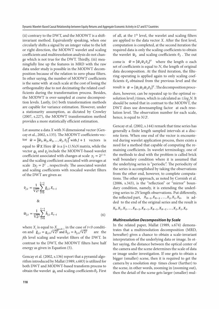
(ii) contrary to the DWT, and the MODWT is a shift-invariant method. Equivalently speaking, when one circularly shifts a signal by an integer value to the left or right direction, the MODWT wavelet and scaling coefficients and multiresolution analysis do not chan-ge which is not true for the DWT. Thirdly, (iii) mea-ningfully line up the features in MRD with the raw data under study is possible in the MODWT decom-position because of the relation to zero-phase filters. In other saying, the number of MODWT coefficients is the same with at each scale at the cost of losing the orthogonality due to not decimating the related coef-ficients during the transformation process. Besides, the MODWT is over-sampled at coarse decomposi-tion levels. Lastly, (iv) both transformation methods are capable for variance estimation. However, under a stationarity assumption, as dictated by Crowley (2007, s.227), the MODWT transformation method provides a more statistically efficient estimation.

Let assume a data X with N dimensional vector (Gen-cay et al., 2002, s.135). The MODWT coefficients vec-tor

equal to . Here is a (j+1) NxN matrix, while the vector and include the MODWT-based wavelet coefficient associated with changes at scale and the scaling coefficient associated with averages at scale , respectively. The associated wavelet and scaling coefficients with rescaled wavelet filters of the DWT are given as:

&

where Xt is equal to Xtmodt-1 in the case of t<0 conditi-on and are the jth level scaling and wavelet filters of the DWT. In contrast to the DWT, the MODWT filters have half energy as given in Equation (5).

Gencay et al. (2002, s.136) report that a pyramid algo-rithm introduced by Mallat (1989, s.683) is utilized for both DWT and MODWT-based transform process to obtain the wavelet and scaling coefficients . First

of all, at the 1th level, the wavelet and scaling filters are applied to the data vector X. After the first level, computation is completed, at the second iteration the required data is only the scaling coefficients to obtain the wavelet and scaling coefficients . The out

come is where the length o each set of coefficients is equal to N, the length of original data decomposition. At the third iteration, the filte-ring operating is applied again to only scaling coef-ficients obtained from the previous level and the result isdure, however, can be repeated up to the optimal re-solution level j times, which is calculated as ≤log2N. It should be noted that in contrast to the MODWT, the DWT does use downsampling factor at each reso-lution level. The observation number for each scale, hence, is equal to N/2j.

Gencay et al. (2002, s.144) remark that time series has generally a finite length sampled intervals at a disc-rete form. When one end of the vector is encounte-red during wavelet application process, there exists a need for a method that capable of computing the re-maining coefficients. In wavelet terminology, one of the methods to deal with the problem is called brick wall boundary condition where it is assumed that the underlying series is “periodic”. The periodicity of the series is accomplished by taking the observations from the other end, however, to complete computa-tions. The other approach, as noted by Cornish et al. (2006, s.343), is the “reflection” or “mirror” boun-dary condition, namely, it is extending the underl-ying series to 2N length observations. Put differently, the reflected part, is ad-ded to the end of the original series and the result is

Multiresolution Decomposition by Scale In the related paper, Mallat (1989, s.674) demons-trates that a multiresolution decomposition (MRD, hereafter) gives a chance to obtain a scale-invariant interpretation of the underlying data or image. In ot-her saying, the distance between the optical center of the camera and the scene determines the scale of data or image under investigation. If one gets to obtain a bigger (smaller) scene, then it is required to get the camera by a resolution step times closer (further) to the scene, in other words, zooming in (zooming out), then the detail of the scene gets larger (smaller) mul-

𝑤𝑤 = 𝑤𝑤#,𝑤𝑤%, 𝑤𝑤&, … ,𝑤𝑤(, 𝑣𝑣(*with 𝐽𝐽 + 1 vectors is

𝑊𝑊𝑋𝑋 𝑊𝑊𝑋𝑋 𝑤𝑤" 𝑣𝑣"

𝛾𝛾" = 2"%&

2𝛾𝛾# = 2#

𝑣𝑣",$ =12"( g",*

+,-

*./

𝑋𝑋$,*&𝑤𝑤",$ =12"( ℎ",*

+,-

*./

𝑋𝑋$,*

𝑣𝑣",$ =12"( g",*

+,-

*./

𝑋𝑋$,*&𝑤𝑤",$ =12"( ℎ",*

+,-

*./

𝑋𝑋$,* (6)

g",$ = g",$ 2"' and ℎ",$ = ℎ",$ 2"'

𝑤𝑤" 𝑣𝑣"

𝑤𝑤" 𝑣𝑣"

𝑤𝑤 = 𝑤𝑤#𝑤𝑤$𝑣𝑣$ &

𝑣𝑣"

𝑤𝑤 = 𝑤𝑤#𝑤𝑤$𝑤𝑤%𝑣𝑣% ' . The decomposition proce-

𝑋𝑋"#$, 𝑋𝑋"#&, … , 𝑋𝑋&, 𝑋𝑋$, 𝑋𝑋),

𝑋𝑋", 𝑋𝑋$, 𝑋𝑋%, … , 𝑋𝑋'(%, 𝑋𝑋'($, 𝑋𝑋'($, 𝑋𝑋'(%, … , 𝑋𝑋%, 𝑋𝑋$, 𝑋𝑋".



tiplied by for each step. Putting differently, Hubbard (2005, s.137) reports that the MRD tool enables rese-archers to simultaneously attain both the details and the overall picture of the data which seems as if the camera is come closer and then moved away.

In MRD analysis, the transformation process is perfor-med via the pyramid (cascade) algorithm introduced by Mallat (1989, s.685) which enables to zoom in on scaling function (Daubechies, 1992, s.3). Therefore, the multire-solution approximation of an underlying X(t) variable, as reported by Ramsey (2014, s.12), is formulated as follows:

)7(

𝑆𝑆" t = 𝑆𝑆",&&

𝜙𝜙",& t &𝐷𝐷+ t = 𝑑𝑑+,&𝜓𝜓+,& t&

𝑋𝑋 𝑡𝑡 = 𝑆𝑆" t + 𝐷𝐷+ t"

+12

or𝑋𝑋 𝑡𝑡 = 𝐷𝐷2 𝑡𝑡 + ⋯+ 𝐷𝐷"67 𝑡𝑡 + 𝐷𝐷"62 𝑡𝑡 + 𝐷𝐷" 𝑡𝑡 + 𝑆𝑆" 𝑡𝑡 (1)

where Dj(t), observed at j=1, ... ,J, parameters inclu-de the detail components at an increasingly finer re-solution level, while the Sj(t) parameter includes the smooth component of the series under investigation. Gallegati et al., (2017, s.8) remark that the detail com-ponent denotes the scale deviation from the smooth process, namely, it is the degree of difference of the observations of the series at each individual resolu-tion level, while the smooth component provides the smooth long-term behavior of the underlying series. Therefore, due to the feature of additive decomposi-tion, it is easy to reconstruct the original series, X(t), by summing up the detail and smooth components.

To be more precise, let us give an example of the MRD process with six different j= 2,...,7 resolution levels based on MODWT approach. For the purpose

of brevity, only the MRD of the first observation, , of “US_DLIP” variable is given in Table 2. It is evident that the details coefficients remain the same, while the smooth coefficient is decomposed into two parts at each resolution level due to orthogonality property of the wavelet filter. Equivalently saying, the decom-position process focuses only on the nonstationary coefficients of the series until the optimal resolution level is reached. Therefore, the sum of the detail and the smooth coefficient of scale d3, for example, will be equal to the smooth coefficient of s2. At each sca-le, if one adds these two coefficients, then, the result will be the first observation . This is also true for all other observations, namely, if one sums their details and smooth coefficients, for example at scale d5, the result will yield the original time series as US_DLIP= d1+d2+d3+d4+d5+s5.

J d1 d2 d3 d4 d5 d6 d7 sj 2 0.00294979 -0.00072004 [s2] -0.00105176 3 0.00294979 -0.00072004 -0.00182575 [s3] 0.00077399 4 0.00294979 -0.00072004 -0.00182575 -0.0011589 [s4] 0.00193288 5 0.00294979 -0.00072004 -0.00182575 -0.0011589 -0.00013675 [s5] 0.00206963 6 0.00294979 -0.00072004 -0.00182575 -0.0011589 -0.00013675 0.00091154 [s6] 0.00115809 7 0.00294979 -0.00072004 -0.00182575 -0.0011589 -0.00013675 0.00091154 0.00010809 0.00105

Source: Author’s calculation.

Table 2. Multiresolution decomposition (MRD) with different resolution levels

Source: Author’s calculation

120


Wavelet Variance, Covariance, and Correlations by Scale

In this section, we will give brief information about the MODWT based wavelet variance, covariance, correlation and cross-correlation measure.

The first concept is the wavelet-based variance mea-sure. Percival and Walden (2000, s.296) demonstrate that wavelet variance is a practical concept for both stationary process and nonstationary process having stationary backward differences for the underlying sample variance. On the other hand, Percival (1995, s.621) describes the wavelet variances as a particular part of total sample variance, namely, the sample va-riance is broken down into several components asso-ciated with scales. Equivalently speaking, Lindsay et al. (1996, s.778) say that using wavelets one can stra-ightforwardly decompose the sample variance into a scale-by-scale basis, leading to both the notion of the scale-dependent wavelet variance estimation and determination of the locations of the events contribu-ting to the total sample variance at each time horizon or frequencies.

In wavelet literature, it is widely known that the wave-let variance is treated as energy decomposition. Beca-use each wavelet detail coefficients have a zero-mean, as noted by Crowley (2007, s.228), the variance analy-sis is regarded as energy decomposition. Due to the energy preserving property of the MODWT transfor-mation, as Gallegati and Ramsey (2013, s.187) report, the sum of the energies of the two wavelet and scaling coefficients is equal to the total energy of the original time series. Percival and Mofjeld (1997, s.872) provi-de the energy decomposition of wavelet analysis as given

where and denotes wavelet and scaling coeffi-cients derived from MODWT transform process, respectively. The wavelet coefficients detain the vari-ations of the underlying time series from its long-run average value at each scale.

Regarding statistically significant results, Whitcher (1998, s.107) provides the unbiased estimator of the

(time-independent) wavelet variance based upon the MODWT for each scale, in Equation (9) with the following conditions for a stationary or nonstationary variable

where

denote the wavelet filter length and the number of co-efficients unaffected by the boundary conditions for each scale λj decomposition of the underlying variab-le. However, Gencay et al. (2002, s.137) remark that since the related wavelet filter is a rescaled version of the DWT wavelet filter, a normalization factor 2λj is not necessary in the case of the MOWT.

It is noteworthy that the number of the MODWT() and MRA() coefficient is equivalent to the length of the time series in the case of MODWT on the cont-rary to DWT approach. However, the number of the MODWT() coefficients are scale-dependent due to boundary conditions, namely, as scale increases the number of useful coefficients decreases.

It is easy to derive the wavelet covariance scale-by-scale between two time series of interest after wavelet variances are calculated. Cornish et al. (2006, s.363) define the wavelet covariance as a measure of the deg-ree of simultaneous correlation between two wavelet crystals for each scale. Gencay et al. (2001, s.254) state that the unbiased estimator of the wavelet covariance based upon MODWT() can be described as the cova-riance between the wavelet scale of X and Y as follows

Providing a unique technique for attributing levels of relationship with different time horizons, as noted by Gencay et al. (2001, s.255), the wavelet covarian-ce gives an ability to determine which wavelet scale (or time horizon) are significantly contributing to the covariance relationship between the underlying time series during the sample period.

It is widely known that the covariance measure does not take into consideration, as dictated by In and Kim (2012, s.32) of the strength of the association. Hen-

𝑋𝑋 " = 𝑤𝑤%"

&

%'(

+ 𝑣𝑣%"; 𝑓𝑓𝑓𝑓𝑓𝑓𝑗𝑗 ≥ 1;

(8)

𝑤𝑤" 𝑣𝑣"

𝜆𝜆" = 2"%&

𝜎𝜎"# 𝜆𝜆% =1𝑁𝑁%

𝑤𝑤%,+#,-.

+/01-.

(9)

𝐿𝐿" = 𝐿𝐿 − 1 ∗ (2" − 1) + 1 and 𝑁𝑁" = 𝑁𝑁 − 𝐿𝐿" + 1

𝛾𝛾",$ 𝜆𝜆& =1𝑁𝑁*

𝑊𝑊",*,,𝑊𝑊$,*,,

-./

,012./

(10)



ce, it is required to turn our attention to the wave-let correlation terminology. Despite indicating a co-movement between wavelet scales of two time series up to some extent, the wavelet correlation would be a more suitable analyzing tool with regard to wave-let covariance. Whitcher (1998, s.115) introduces the wavelet correlation measure between the wavelet sca-le, λi, based upon unbiased MODWT() coefficients of the underlying bivariate time series as

where given in the numerator Equation (11) is covariance between two time series and given in the denominator are the square root of the wavelet variance of X and Y, res-pectively.

Because of intrinsic non-normality of the correlation measure in the case of small-sized samples, Gencay et al. (2001, s.256) document that, it is sometimes requ-ired to use a nonlinear transformation, i.e., Fisher’s z transform, to build a confidence interval for the esti-mated wavelet correlation, , for each scale decom-position as given in Equation (12)

where the transformed and unbiased estimated correlation coefficient is based on independent samples. Whitcher et al. (2000, s.14947) state that

has approximately a N(0,1) dist-ribution. For a better approximation of the distributi-on, however, the factor is used in calculation of the confidence intervals given in Equation (13) and the transformation factor. According to Gencay et al. (2002, s.241) it maps the confidence interval back to between [-1] and [+1] to generate an approxima-

te 100(1-2p)% confidence interval based upon DWT coefficients. The reason behind using DWT instead of MODWT is to obtain more realistic confidence intervals. Gencay et al. (2001, s.256) remark that the CIs do not exploit any information about whether it is distributed by Gaussian or non-Gaussian condition.

After calculating wavelet correlation, it is natural to derive the wavelet cross-correlation coefficients for each wavelet scale. Whitcher (1998, s.115) introduce MODWT based cross-correlation measure for each scale λ at lag τ as

Gencay et al. (2002, s.258) report that this analy-sis method, just as in the case of standard cross-correlation, can be used to measure lead/lag relati-onships between two time series. Besides, at zero lag, τ=0, the cross-correlation measure will be equal to basic wavelet correlation coefficient. Whitcher (1998, s.122) reminds that the magnitude of the wavelet cor-relation and cross-correlation coefficients are boun-ded .

Econometric MethodologyIn line with the main objective, the cointegration and causal relationships are measured by both the stan-dard and frequency-based analyzing tools. The first challenging step is examining whether the underlying variables are stationary or not. The stationarity is de-fined by Gujarati and Porter (2004, s.797) as two main moments, mean and variance, are unchanged during the sample period and the covariance depends only upon the time intervals or lags not the actual time. If a time series is not stationary, then it is said that it fol-lows a random walk or it has a unit root. The first ma-jor consequence of the using nonstationary variable is that, as noted by Brooks (2014, s.354), the model re-sult may be spurious, namely, they cannot be trusted. In addition, the standard assumption for asymptotic analysis is invalid, i.e. the t-ratios and F-statistics do not follow t-distribution and F-distribution, respec-tively. After determining the integration order of the variable, the next step is to investigate the cointegra-tion orders.

𝜌𝜌",$ 𝜆𝜆& =𝛾𝛾",$ 𝜆𝜆&

𝜎𝜎" 𝜆𝜆* ∗ 𝜎𝜎$ 𝜆𝜆* (11)

𝛾𝛾",$ 𝜆𝜆&

𝜎𝜎" 𝜆𝜆$ and 𝜎𝜎% 𝜆𝜆$

𝜌𝜌

h 𝜌𝜌 =12 𝑙𝑙𝑙𝑙𝑙𝑙

1 + 𝜌𝜌1 − 𝜌𝜌 = tanℎ/0(𝜌𝜌) (12)

tanℎ ℎ 𝜌𝜌&' 𝜆𝜆) −𝛷𝛷,-(1 − 𝑝𝑝)

𝑁𝑁) − 3, tanℎ ℎ 𝜌𝜌&' 𝜆𝜆) +

𝛷𝛷,-(1 − 𝑝𝑝)

𝑁𝑁) − 3

tanℎ ℎ 𝜌𝜌&' 𝜆𝜆) −𝛷𝛷,-(1 − 𝑝𝑝)

𝑁𝑁) − 3, tanℎ ℎ 𝜌𝜌&' 𝜆𝜆) +

𝛷𝛷,-(1 − 𝑝𝑝)

𝑁𝑁) − 3

(13)

𝑁𝑁 − 3[ℎ(𝜌𝜌) − ℎ(𝜌𝜌)]

𝑁𝑁 − 3

(14)𝜌𝜌",$,% 𝜆𝜆' =𝛾𝛾",$,% 𝜆𝜆'

𝜎𝜎",$ 𝜆𝜆+ ∗ 𝜎𝜎",% 𝜆𝜆+

𝜌𝜌",$,% 𝜆𝜆' ≤ 1

122


The cointegration or long-run relationship frame-work is introduced by Granger (1981, s.128) where it is defined in terms of reduction of the order of integ-ration. If two series are both found to be stationary at the same integration order, , then their linear combi-nation is stationary as well. The result of cointegra-ting vector leads to examine the possible relationship by including an error correction term in vector au-toregressive (VAR) model. Thus, the existence of co-integrating vector(s) implies at least one-way causal relationship in the long run. If not, then the causality is tested by a standard VAR model. The causal relati-onship is introduced by Granger (1969, s.429) as to test whether the lagged information of stationary X variable is helpful in predicting the current values of stationary Y or not.

Lee and Strazizich (2003) Unit Root TestBrooks (2014, s.365) states that if a test does not take into account possibility of structural breaks, in case of a larger break and a small-sized sample, test po-wer, therefore, will reduce; namely, it might tend to reject the null hypothesis straightforwardly when actually it is correct. In econometric literature, the first test that takes the structural breaks into account is the test of Perron (1989) where the test permits a one-time change in level or trend. In this test, the change point, however, is determined exogenously by the researchers. After the Perron (1989) test, several unit root tests with structural breaks are introduced by different researchers. However, some important problem occurs when interpreting test results with structural breaks, as dictated by Lee and Strazizich (2003) in their paper, because these tests do not allow for breaks both in the null and alternative hypothesis. They (2003, s.1082) report that if a test does not sup-pose break(s) under the null, the test statistic might diverge and may cause significant rejections of the null hypothesis. Therefore, they (2003) offer a unit root test where it permits for two change points and the rejection of the null entails that the time series under study is trend-stationary. They (2003, s.1083) establish two different models: “Model A” includes two shifts in level and “Model C” allows two shifts in level and trend. For the unit root testing, Lee and Strazizich (2003, s.1083) suggest using the regression of ror term is . The essential regression to calculate the two-breakpoint LM test statistic is gi-ven as

where , observed at .

Hence, the null hypothesis is determined as testing .

Hacker and Hatemi (2006) Symmetric Causality TestIn the case of different integration orders of variab-les, researchers have commonly preferred implemen-ting the Toda and Yamamoto (1995) approach since last two decades due to its simplicity and being free of conduction cointegration tests. However, as poin-ted out by Hacker and Hatemi-J (2006, s.1490), the Toda and Yamamoto (1995) approach is sensitive for the assumption of normality and the presence of the ARCH effects in the case of small-sized samples. On the other hand, Al Janabi et al. (2010) stated that it is accepted that the financial time series are gene-rally not normally distributed. Hence, Hacker and Hatemi-J (2006, s.1492) remark that the Wald test statistics generated by Monte Carlo simulation results can be biased. They (2006) offer a modified version of the Toda and Yamamoto (1995) approach where the critical values of MWALD test are generated by leveraged bootstrap simulation technique to remedy the problems mentioned before.

Hacker and Hatemi-J (2006, s.1490) propose using the same augmented VAR (p+d) model that Toda and Yamamoto (1995) offer for using test of causality

where p denotes the optimal lag order of the model determined beforehand and d represents the maxi-mum integration order of the variables under study. If the th parameter of dependent variable of Yt does not lead the kth parameter of dependent variable of Yt, then the null hypothesis H0 cannot be rejected, where H0 is that the row k column j parameter in βz is equi-valent to zero with the condition of z=1, ..., p. As no-ted by Toda and Yamamoto (1995, s.227), adding the parameters for the extra lag(s) in causality test is to guarantee the use of asymptotical distribution theory.

The required VAR (p+d) model including a constant term is described as w h e r e

𝑋𝑋" = 𝜗𝜗′𝑊𝑊" + 𝜖𝜖" 𝜖𝜖" = 𝛽𝛽𝜖𝜖"%& + 𝜐𝜐"

𝜐𝜐"~iid𝑁𝑁 0, 𝜎𝜎* where and er-

∆𝑋𝑋# = 𝜗𝜗′∆𝑊𝑊# + ∅𝑅𝑅#*+ + 𝑢𝑢# (15)

𝑅𝑅" = 𝑋𝑋" − 𝜔𝜔' −𝑊𝑊"𝜗𝜗 𝑡𝑡 = 2,3, …𝑇𝑇

∅ = 0

𝑌𝑌" = 𝛾𝛾 + 𝛽𝛽'𝑌𝑌"(' + 𝛽𝛽)𝑌𝑌"() + ⋯+ 𝛽𝛽+𝑌𝑌"(+ + ⋯+ 𝛽𝛽+,-𝑌𝑌"(+(- + 𝑢𝑢"

𝑌𝑌" = 𝛾𝛾 + 𝛽𝛽'𝑌𝑌"(' + 𝛽𝛽)𝑌𝑌"() + ⋯+ 𝛽𝛽+𝑌𝑌"(+ + ⋯+ 𝛽𝛽+,-𝑌𝑌"(+(- + 𝑢𝑢" (16)

𝑌𝑌 = 𝑀𝑀𝑊𝑊 + 𝑢𝑢,



is an matrix. They (2006, s.1491) suggest using the follo-wing modified Wald (MWALD) test statistic

where and C denote the Kronecker product and a matrix, respectively. Besides, in

Equation (17) is equal to vec(M) and if the related parameter in is zero, then C is equal to one or zero otherwise. The null hypothesis of non-causality is for-mulated as . However, it is convenient at this point to remark that, the MWALD test statistic used for this approach is assumed to be asymptoti-cally X2 distributed where the number of degrees of freedom is equal to the number of restrictions, p.

𝑀𝑀 ∶= (𝛾𝛾, 𝛽𝛽(, … , 𝛽𝛽*, … , 𝛽𝛽*+,) (𝑛𝑛x(1 + 𝑛𝑛 𝑘𝑘 + 𝑑𝑑 ))

MWALD&& = 𝐶𝐶𝜗𝜗 ′ 𝐶𝐶 𝑊𝑊 ′𝑊𝑊 +, ⊕+𝑆𝑆0 𝐶𝐶 ′ +, 𝐶𝐶𝜗𝜗 ~𝜒𝜒34

MWALD&& = 𝐶𝐶𝜗𝜗 ′ 𝐶𝐶 𝑊𝑊 ′𝑊𝑊 +, ⊕+𝑆𝑆0 𝐶𝐶 ′ +, 𝐶𝐶𝜗𝜗 ~𝜒𝜒34 (17)

⊕ 𝑝𝑝x𝑛𝑛 1 + 𝑛𝑛 𝑝𝑝 + 𝑑𝑑

𝜗𝜗 𝜗𝜗

𝐻𝐻": 𝐶𝐶𝜗𝜗 = 0

Table 3. Unit Root Test Results with the Standard Methods

Variable Level (C+T) Difference (C+T)

ADF KPSS PP ADF KPSS PP US_LIP -3.4361 ** 0.108 -2.4800 -3.8969 ** 0.0549 -14.0945 *** US_LSE -1.8355 0.255 *** -1.9949 -14.5025 *** 0.0577 -14.4853 *** GER_LIP -3.4723 ** 0.0637 -3.0043 -6.0547 *** 0.0337 -17.3118 *** GER_LSE -2.0476 0.2285 *** -2.0476 -13.9916 *** 0.0481 -13.9916 *** ENG_LIP -2.2662 0.1693 ** -2.0741 -18.1581 *** 0.1085 -18.1975 *** ENG_LSE -1.9348 0.1996 ** -2.1218 -15.1729 *** 0.047 -15.1785 *** JAP_LIP -3.3409 * 0.1538 ** -3.0137 -13.5031 *** 0.0344 -13.5880 *** JAP_LSE -1.3944 0.2154 ** -1.7056 -13.5457 *** 0.0518 -13.6035 *** FRA_LIP -1.9203 0.1406 * -2.6256 -21.7076 *** 0.0779 -20.9190 *** FRA_LSE -2.2936 0.0931 -2.6388 -13.5107 *** 0.0827 -13.5183 *** ITA_LIP -2.7107 0.2064 ** -2.3556 -6.4969 *** 0.075 -17.7270 *** ITA_LSE -2.6079 0.1089 -2.8702 -14.5528 *** 0.0848 -14.5781 *** CAN_LIP -1.9531 0.1805 ** -2.3218 -13.9521 *** 0.1204 * -14.3050 *** CAN_LSE -2.9566 0.1111 -2.9003 -12.1332 *** 0.0304 -12.1496 *** TUR_LIP -2.5929 0.1709 ** -2.8005 -19.4879 *** 0.0763 -19.4354 *** TUR_LSE -2.6874 0.2944 *** -2.7985 -15.5559 *** 0.0262 -15.5562 *** BRA_LIP -1.1493 0.4032 *** -1.1493 -16.4468 *** 0.0452 -16.4468 *** BRA_LSE -1.7832 0.3604 *** -1.8813 -14.7195 *** 0.0511 -14.7185 *** RUS_LIP -1.7401 0.3892 *** -1.9286 -18.6728 *** 0.043 -18.7693 *** RUS_LSE -2.0508 0.4285 *** -1.8474 -13.0636 *** 0.0324 -13.0770 *** MEX_LIP -2.5274 0.0703 -2.7785 -17.6884 *** 0.0464 -17.4794 *** MEX_LSE -1.6769 0.326 *** -1.8027 -15.1441 *** 0.0773 -15.1447 *** INDO_LIP -1.4578 0.3548 *** -13.0883 *** -7.9090 *** 0.1509 ** -93.0774 *** INDO_LSE -2.8812 0.1832 ** -2.3956 -12.4649 *** 0.0582 -12.4649 *** IND_LIP -0.4727 0.3804 *** -1.1235 -15.1634 *** 0.1141 -24.1820 *** IND_LSE -2.1727 0.1699 ** -2.4799 -14.5803 *** 0.0605 -14.6561 *** SAFR_LIP -2.2905 0.2458 *** -2.8131 -21.7656 *** 0.0364 -22.0717 *** SAFR_LSE -2.4283 0.1656 ** -2.5455 -16.0876 *** 0.0397 -16.0877 ***

Empirical ResultsThis section is divided into two groups where the first part includes the econometric test results both in the time and frequency domain. The second part comp-rises the wavelet-based statistics.

Wavelet-Based Econometric Test ResultsThe first step in the econometric analysis is the unit root testing of variables. In this paper, at first we test the nonstationarity with three conventional unit root tests of the ADF, PP, and KPSS and report it in Tab-

124


le 3. Note that, the null hypothesis of the ADF and PP test is different from the null hypothesis of the KPSS test. Table 3 shows that all variables, with the exception of the “US_LIP”, “GER_LIP”, “JAP_LIP”, and “INDO_LIP”, have unit root in log-level accor-ding to the ADF and PP test. To robustness check, the KPSS test is implemented as well. The null hypothe-sis of stationary for the KPSS test is not rejected for six out of the twenty-eight variables, where the ADF and PP test results of the “US_LIP” and “GER_LIP” are confirmed. Note that all stock markets are found to be nonstationary, according to the ADF and PP, indicating that they are efficient in the weak-form. On the other hand, all variables become stationary at the first-differenced, except the “CAN_LIP” and “INDO_LIP” regarding the KPSS. Consequently, it can be said that all variables with two exceptions are integrated of order one, .

Evidently, the different tests without structural breaks yield different results. However, not including struc-tural breaks might lead to spurious/biased results. Hence, the modern L&S (2003) unit root test with two unknown structural breaks is conducted to obta-in the final results, reported in Table 4.

Table 4 shows that the twelve out of the twenty-eight variables are found to be stationary with two breaks in log-levels. Note that the “CAN_LIP” and “INDO_LIP” variables are stationary at significance level in the first log-differenced. These results imply that only the E7 countries of the “TUR_LSE”, “BRA_LSE”, “RUS_LSE”, “MEX_LSE”, and “IND_LSE” stock mar-kets are not weak-form efficient, namely, they do not follow a random walk. Therefore, the cointegration process is required for only “ITA” and “CAN” country variables.

Table 4. Unit Root Tests with the L&S (2003) ApproachG7 Countries

Model C E7 Countries

Model C LM test BP1 BP2 LM test BP1 BP2

US_LIP -5.758 ** 2008-Jun 2011-Feb TUR_LIP -4.519 2002-Oct 2008-Aug US_LSE -4.677 2003-Feb 2008-Sep TUR_LSE -6.717 *** 2001-Dec 2005-Dec GER_LIP -5.798 ** 2004-Nov 2008-Sep BRA_LIP -5.126 2006-Sep 2015-Jan GER_LSE -4.500 2002-Mar 2006-May BRA_LSE -6.090 ** 2002-May 2008-May ENG_LIP -6.963 *** 2008-Sep 2014-Sep RUS_LIP -4.491 2001-Apr 2006-May ENG_LSE -4.037 2002-Sep 2008-Aug RUS_LSE -6.282 ** 2005-Oct 2008-Aug JAP_LIP -6.648 *** 2003-Jul 2008-Oct MEX_LIP -4.055 2001-Jun 2005-Jun JAP_LSE -3.223 2005-May 2009-Feb MEX_LSE -5.596 * 2003-Mar 2008-Jul FRA_LIP -6.672 *** 2008-Aug 2010-Sep INDO_LIP -7.674 *** 2002-Nov 2005-Nov FRA_LSE -3.917 2002-Mar 2014-Jul INDO_LSE -4.838 2001-Sep 2006-Oct ITA_LIP -5.232 2008-Jul 2011-Aug IND_LIP -4.988 2003-Sep 2008-Aug ITA_LSE -3.565 2010-Apr 2013-Jun IND_LSE -6.141 ** 2003-May 2008-Jun CAN_LIP -5.232 2008-Jul 2011-Aug SAFR_LIP -5.393 * 2008-Mar 2010-Oct CAN_LSE -3.565 2010-Apr 2013-Jun SAFR_LSE -4.613 2002-Nov 2006-Feb

For cointegration analysis, the Hatemi-J (2008) app-roach with two unknown structural breaks is pre-ferred. To take into account the effect of two regime shifts allowed endogenously both in the intercept and the slope parameters during the time period of study, the required model C/S is formulated as given

&

where the dummy variables D1t and D2t with the unk-nown parameters τ1 and τ2 defined represent the relative timing of structural break points. The test statistics of the modified ADF* and modified Philips tests, Zα

* and Zt*, are described as

𝑌𝑌" = 𝑐𝑐% + 𝑐𝑐'𝐷𝐷'" + 𝑐𝑐)𝐷𝐷)" + 𝛽𝛽%′ 𝑋𝑋" + 𝛽𝛽'′𝐷𝐷'"𝑋𝑋" + 𝛽𝛽)′𝐷𝐷)"𝑋𝑋" + 𝑒𝑒"

𝑌𝑌" = 𝑐𝑐% + 𝑐𝑐'𝐷𝐷'" + 𝑐𝑐)𝐷𝐷)" + 𝛽𝛽%′ 𝑋𝑋" + 𝛽𝛽'′𝐷𝐷'"𝑋𝑋" + 𝛽𝛽)′𝐷𝐷)"𝑋𝑋" + 𝑒𝑒" (18)

𝐷𝐷"# =0if𝑡𝑡 ≤ 𝑛𝑛𝜏𝜏"1if𝑡𝑡 > 𝑛𝑛𝜏𝜏"

&𝐷𝐷0# =0if𝑡𝑡 ≤ 𝑠𝑠𝜏𝜏01if𝑡𝑡 > 𝑠𝑠𝜏𝜏0

𝐷𝐷"# =0if𝑡𝑡 ≤ 𝑛𝑛𝜏𝜏"1if𝑡𝑡 > 𝑛𝑛𝜏𝜏"

&𝐷𝐷0# =0if𝑡𝑡 ≤ 𝑠𝑠𝜏𝜏01if𝑡𝑡 > 𝑠𝑠𝜏𝜏0



where T is defined as 0.15n, 0.85n with

The Hatemi-J cointegration test (2008) results are re-ported in Table 5. Obviously, there exists a long-run relationship between the variables of “CAN”, indica-ting that “CAN_LIP” and “CAN_LSE” move in tan-dem in the long run, requiring of studying a causal relationship in VECM. In addition, there are not any cointegrating vectors for “ITA” variables according to the and Zα

* test statistic results

Under the cointegration results, VECM based causal relationship test results are given in Table 6. The re-

sults represent a negative significant unidirectional long-run relationship from “CAN_LSE” to “CAN_LIP”. The speed of the adjustment parameter -0.027 reveals that the disequilibrium in the “CAN_LIP” is corrected in 37 months. Besides, a bidirectional Granger causal link is obtained between the “CAN_LIP” and “CAN_LSE” in the short-run at different, and , significance level. This finding partially rein-force the results of Choi et al. (1999) where one-way causalities running from quarterly stock returns to industrial production growth rate are detected in the G7 countries of the “U.S.”, “GER”, “UK”, “JAP”, “FRA”, and “CAN” in the short-run.

𝐴𝐴𝐴𝐴𝐴𝐴∗ = inf)*,), ∈.

𝐴𝐴𝐴𝐴𝐴𝐴 𝜏𝜏0, 𝜏𝜏1 ; 𝑍𝑍5∗ = inf)*,), ∈.

𝑍𝑍5 𝜏𝜏0, 𝜏𝜏1 ; 𝑍𝑍6∗ = inf)*,), ∈.

𝑍𝑍6 𝜏𝜏0, 𝜏𝜏1 (19)

𝜏𝜏" ∈ 𝑇𝑇" = (0.15, 0.70) and 𝜏𝜏" ∈ 𝑇𝑇" = (0.15 + 𝜏𝜏,, 0.85).

Table 5. Hatemi-J Cointegration Test (2008) Results

Model (Dependent ~ Independent)

ADF* Philips Za* Test Stat BP1 BP2 Test Stat BP1 BP2

ITA_LIP ~ ITA_LSE -5.024 2006-11-30 2011-01-31 -45.023 2007-10-31 2008-07-31 CAN_LIP ~ CAN_LSE -5.983 * 2001-10-31 2006-02-28 -62.178 * 2001-11-30 2006-03-31 ITA_LSE ~ ITA_LIP -5.186 2000-12-22 2005-05-31 -41.459 2000-12-22 2005-05-31 CAN_LSE ~ CAN_LIP -6.503 ** 2002-02-28 2003-08-29 -74.432 * 2002-02-28 2003-10-31

Table 7 documents the causality test results using the “MSBVAR” package developed by Brandt (2009) both in the time and in frequency domain using well-specified VAR models. Evidently, there exist bidirec-tional causal relationships between the underlying variables for the “U.S.”, “UK”, “JAP”, “FRA”, “RUS”, and “SAFR” countries, indicating that both variables

have a great impact on each other during the samp-led period. The one-way causal links running from stock markets to industrial production index, in ad-dition, in time domain suggest that the stock markets of “GER”, “ITA”, “TUR”, “BRA”, “MEX”, “INDO”, and “IND” countries are semi-strong efficient according to both unit root and VAR causality test results.

Model SE ⇏ IP

Model IP ⇏ SE

𝜒𝜒# statistics 𝐸𝐸𝐸𝐸𝐸𝐸'() 𝜒𝜒# statistics 𝐸𝐸𝐸𝐸𝐸𝐸'()

CAN_LIP~CAN_LSE 23.508 *** -0.027 ** CAN_LSE~CAN_LIP 12.771 ** -0.001

Table 6. VECM Granger Causality Test

126


In order to test whether there exists a Granger-causa-lity between the stock markets and industrial produc-tion at different investment horizon, the MODWT MRA() coefficients are utilized. The wavelet scales obtained via the LA(8) wavelet filters and “periodic condition” are the scales d1, d2, d3, d4, and d5 re-lated to [2–4), [4–8), [8–16), [16–32), and [32–64) monthly time periods, respectively.

The last five column in Table 7 shows that there are feedback relationships between two variables for all countries, where the rejection of the null hypothe-sis is scale-dependent. For example, the “TUR_LIP” does not Granger causes the “TUR_LSE” regarding the time domain results, however, it is observed that time-dependent causal relationships are hidden bet-ween the wavelet scales of d2 and d5, namely the “TUR_LIP” does Granger causes the “TUR_LSE” af-ter 4 months. In addition, the stock market return Granger causes the industrial production growth rate up to scale d4 in “ITA”, however, the reversal link starts at scale d2.

The test results of both methods for the “U.S” case are partly in line with the paper of Kim and In (2003). They (2003, s.14) state that, at first they failed to find out a feedback causal relationship in the time doma-in. However, they report time-dependent results in the wavelet approach. With the aid of the wavelets, it is found that the lagged industrial production growth rate had a significant effect on the stock returns, which is not observable in the standard method. Ove-rall, they (2003) showed that there exist bidirectional relationships at short and long-term, corresponding to scale d1, d2, d5, and s6.

In addition to standard causality test, we also con-ducted the symmetric causality test introduced by Hacker and Hacker and Hatemi-J (2006). Notable, the test is conducted for all countries regardless of the existence of cointegration results. To calculate the critical values, 5.000 bootstrap simulations are per-formed; the optimal lag length is determined by the Hatemi-J (2003) information criterion for the mo-dels depending upon the first-differenced data. The symmetric causality test results according to the time and frequency domains are documented in Table 8.

In the time domain, it is evident that there are two-way causal relationships for the “U.S.”, “GER”, and “JAP”, suggesting a non-efficient stock market for

these countries. Remarkably, the number of the ef-ficient markets was seven for the standard Granger test; however, with the symmetric test it is obser-ved that “FRA”, “ITA”, “CAN”, “TUR”, “BRA”, “RUS”, “MEX”, and “SAFR” stock markets are informatio-nally efficient in the semi-strong form. However, the wavelet-based test shows different results from the conventional Granger test. For instance, using stan-dard test a bidirectional causal relationship was found between the scale d3, d4 and d5 for “TUR” during the time period, but, the two-way relationship is not valid anymore at scale d5 in the case of the Hacker and Hatemi-J (2006) approach. Likewise, there exist strong evidence of the bidirectional causal relations-hips at scale d1, d3, d4, and d5 for “U.S.”; between scales of scale d2-d5 for “UK” and “MEX”; at sca-le d2, d3, and d5 for “RUS”; at scale d4 and d5 for “BRA”; and at scale d2, i.e. [4-8) month periods for “ITA”. In addition, thanks to the wavelet approach it is explored that actually the industrial growth rates had a significantly great impact on stock market returns between 4 and 64 monthly periods in “ITA”, “RUS”, “MEX”, “INDO” and “IND” countries, while it was true for “FRA” and “CAN” countries in the time pe-riod of [8-64) months. Hence, it can be said that with the wavelets, it is easy to uncover the true relationship that is hidden among the different time oscillations.

The papers that fully corroborate our findings re-garding bidirectional causalities in the short and/or long-run are prepared by Hassapis and Kalyvitis (2002) and Tsouma (2009) for the “U.S.” and “UK”; and Ratanapakorn and Sharma (2007) for the “U.S.”. The partially confirmed papers, however, are do-cumented by Wongbangpo and Sharma (2002) for “INDO”; Singh (2010) and Kumar and Puja (2012) for “IND”, suggesting a feedback causal effects on each other. On the other hand, regarding unidirec-tional causality from “SE” to “IP” is fully confirmed by Hassapis and Kalyvitis (2002) and Tsouma (2009) for all countries with exceptions for the “U.S.”, “UK”, “RUS”, and “IND” countries. Besides, Duca (2007) for the “U.S.”, “UK”, “JAP”, and “FRA”; Kaplan (2008), Büyüksalvarci and Abdioglu (2010), and Özer et al. (2011) for “TUR”; Panopoulou (2009) for “GER”, “FRA”, and “ITA”; Muradoglu et al. (2000) for “MEX” and “IND” report a significantly causal impact on in-dustrial production growth rate over the sample peri-od, indicating that stock market return improves pre-dictability of the output for the mentioned countries.



In addition, our findings are in line with the results obtained by Şentürk et al. (2014) for “TUR” where equity return is found to be a significant predictor for industrial growth rate at high-frequency point

and high frequency points, on, Tiwari et al. (2015) also report the same outcome, one-way causality from stock market performance to industrial growth rate, for “IND” country at low frequency corresponding to a wave length of more than 15.7 months over the time period of 1993M04-2011M01 after conditioning the VAR model, suggesting to implement economic policies focused on the stock market development. Besides, Croux and Reusens (2013, s.99) corrobo-rated these findings for the G7 countries, using qu-arterly data for the period 1991Q1–2010Q2. It is observed that the slowly fluctuating components of the equity returns have significant and great predic-

tive power for the future output growth at signifi-cance level in all countries. Namely, the null hypot-hesis is rejected only at low frequency intervals corresponding to a wave length of more than 1 year and the average incremental R2 of 8% at the slowly fluctuating component suggests that approximately 8% volatility in the output can be exp-lained by the lagged equity returns.

Wavelet-Based Test ResultsNext, we will discuss the wavelet-based ANOVA sta-tistics test results. For the paper, the monthly return data is decomposed into several wavelet scales via MODWT() approach. Notable, the wavelet computa-tion based on the Daubechies LA(8) wavelet filter is performed with the aid of the “Waveslim” R package introduced by Whitcher (2005). The optimal integer decomposition level is chosen as 5 ≤ log2 (235), altho-ugh, the maximum level is 7.

ranges [0.01 ≤ 𝜔𝜔 ≤ 0.4]

[𝜔𝜔 = 2.5]

[𝜔𝜔 = 1.0, 2.5].

and the opposite is true at both medium

In additi-

[0.01 ≤ 𝜔𝜔 ≤ 1.5]

Model “Stock Return” does not Granger cause “IPI Growth Rate”

Return d1 [2-4) d2 [4-8) d3 [8-16) d4 [16-32) d5 [32-64)

US_DL 10.608 *** 2.105 ** 3.958 *** 2.11 ** 1.022 6.907 *** GER_DL 2.998 ** 1.338 2.149 ** 1.008 1.703 * 10.655 *** ENG_DL 4.77 *** 1.472 1.595 * 2.673 *** 5.092 *** 7.235 *** JAP_DL 1.913 ** 2.668 *** 3.137 *** 3.471 *** 3.751 *** 3.686 *** FRA_DL 4.944 *** 1.557 2.036 ** 1.95 ** 2.114 ** 4.698 *** ITA_DL 5.806 *** 2.233 ** 2.15 ** 0.761 4.328 *** 1.46 CAN_DL NA NA NA NA NA NA

TUR_DL 6.65 *** 2.235 ** 1.516 2.095 ** 5.501 *** 4.506 *** BRA_DL 6.57 *** 2.387 *** 2.255 ** 1.774 * 3.811 *** 3.429 *** RUS_DL 2.918 ** 4.218 *** 4.679 *** 1.497 1.904 ** 2.862 *** MEX_DL 3.607 *** 1.393 2.219 ** 1.928 ** 3.733 *** 2.462 *** INDO_DL 2.361 * 1.461 2.26 ** 2.559 *** 5.163 *** 5.579 *** IND_DL 3.498 ** 2.048 ** 1.98 ** 1.532 3.044 *** 2.668 *** SAFR_DL 4.579 *** 1.238 1.223 0.848 4.847 *** 9.725 ***

Model “IPI Growth Rate” does not Granger cause “Stock Return”

Return d1 [2-4) d2 [4-8) d3 [8-16) d4 [16-32) d5 [32-64) US_DL 2.53 *** 2.029 ** 1.757 * 2.309 *** 4.607 *** 6.37 ***

GER_DL 1.617 0.601 0.675 1.679 * 1.328 8.921 *** ENG_DL 2.073 * 1.638 * 1.466 2.824 *** 4.477 *** 7.187 *** JAP_DL 2.668 ** 0.963 1.592 * 1.613 * 3.529 *** 4.374 *** FRA_DL 2.2 * 1.042 0.526 1.744 * 5.194 *** 6.124 *** ITA_DL 1.336 1.038 1.879 ** 2.253 ** 4.949 *** 4.841 *** CAN_DL NA NA NA NA NA NA TUR_DL 0.522 0.611 2.24 ** 1.886 ** 4.303 *** 5.097 ***

BRA_DL 1.367 1.497 1.79 * 2.438 *** 4.014 *** 4.223 *** RUS_DL 2.317 * 1.294 1.897 ** 2.552 *** 3.114 *** 5.777 *** MEX_DL 0.945 1.345 1.824 ** 2.96 *** 2.878 *** 6.27 *** INDO_DL 1.107 1.01 2.008 ** 2.752 *** 3.325 *** 5.532 *** IND_DL 1.269 1.388 1.189 2.144 ** 2.915 *** 5.303 *** SAFR_DL 1.824 * 0.473 0.667 1.93 ** 4.686 *** 2.823 ***

Table 7. VAR Model Granger Causality Test Results

128


The first wavelet coefficients-based ANOVA statis-tic is the wavelet variance where the coefficients are obtained via the “reflection/mirror condition”. Note that with this method none of the two moment values do not change because of the duplication of the coef-ficients for one time. Notable, the wavelet variance computation is done with the non-boundary “wavelet

coefficients”, where the observation number is 463 at scale d1, 449 at scale d2, 421 at scale d3, 365 at scale d4, and 253 at scale d5 thanks to the “reflection/mir-ror condition”. Note that, if we had preferred the “pe-riodic condition”, however, the observation number at scale d5 would have been 18 indeed.

Table 8. Hacker and Hatemi-J Symmetric Causality Test (2006)

“Stock Return” does not Granger Cause “IPI Growth Rate”

Return d1 [2-4) d2 [4-8) d3 [8-16) d4 [16-32) d5 [32-64)

30.648 *** 30.494 ** 48.324 *** 25.421 ** 25.976 * 90.333 *** 3.408 * 21.170 24.822 * 24.054 * 14.398 68.095 *** 1.728 14.208 26.597 ** 30.413 ** 48.761 *** 49.714 ***

3.757 * 39.751 *** 30.292 ** 38.990 *** 44.254 *** 61.638 *** 5.602 ** 16.357 33.344 ** 23.327 * 52.670 *** 38.139 ***

16.878 *** 23.330 * 23.273 * 18.269 22.406 15.024 15.841 *** 19.057 20.916 50.003 *** 50.356 *** 17.714 ** 11.317 *** 27.900 ** 21.818 34.431 *** 71.144 *** 13.129 16.284 *** 25.062 * 20.197 20.947 38.170 *** 22.870 **

5.219 ** 57.650 *** 71.642 *** 38.835 *** 14.095 26.118 ***

4.778 ** 16.023 35.528 *** 34.679 *** 29.272 ** 37.784 *** 4.303 13.647 21.055 31.147 ** 48.187 *** 24.757 2.350 31.092 ** 24.162 * 25.240 * 17.910 30.148 ** 5.832 ** 12.303 14.907 10.416 53.129 *** 66.562 ***

“IPI Growth Rate” does not Granger Cause “Stock Return”

Return d1 [2-4) d2 [4-8) d3 [8-16) d4 [16-32) d5 [32-64)

17.946 *** 24.559 * 19.937 27.654 ** 62.972 *** 52.331 *** 3.473 * 8.122 6.260 26.846 ** 14.774 43.589 *** 4.211 ** 17.263 26.570 ** 33.713 *** 66.892 *** 52.792 *** 7.775 *** 18.223 19.140 19.301 30.471 ** 41.234 ***

2.086 7.641 16.297 21.039 * 48.508 *** 57.685 *** 0.081 15.156 27.986 ** 29.105 ** 30.344 ** 40.120 *** 0.001 9.338 4.266 29.867 ** 28.718 ** 18.597 ** 0.115 17.835 28.513 ** 28.039 ** 35.650 *** 18.655 1.989 12.275 13.617 27.675 ** 35.298 *** 22.876 ** 1.186 20.532 33.806 *** 29.642 ** 28.345 ** 36.968 *** 1.102 17.372 31.474 ** 34.579 *** 22.908 * 30.084 **

0.549 16.877 30.241 ** 29.067 ** 29.502 ** 73.148 *** 0.862 20.900 23.186 * 28.084 ** 43.300 *** 30.619 ** 1.377 6.010 4.442 22.365 * 66.810 *** 20.073



The unbiased wavelet estimations of the underlying variables are depicted in Figure 2. It is evident that all wavelet variance decreases as wavelet scale increases. First of all, it is not surprising that the volatility of the stock markets is found to be higher than the industrial production in both D7 and E7 countries regardless of the wavelet scales, except at scale d1 in “INDO”. The highest volatility among the equity market returns is observed in Turkey at scale d1. In terms of the energy decomposition, the most contribution to total energy is concentrated in the first finest scales. For example, approximately of the stock market variance is obser-ved in “SAFR” and “TUR” at first scale d1, however, it exceeds at the first two scales, indicating that the most volatility is explained by the short-run fluctuati-ons, d1+d2, in the aforementioned countries.

On the other side, “INDO” has the highest volatility of the industrial production growth observed at sca-le d1 among the countries. The energy decompositi-on reaches to at the first two scales in “INDO”, in “IND”, and in “SAFR”, suggesting that the short-term fluctuations dominate the long-term fluctuations in the case of the energy distribution. These results rein-force the findings of Kim and In (2003, s.13) for the stock markets of G7 where they (2003) suggest taking an action to every price changes in the markets provi-ded that of being a short-time investor.

Figure 2. Wavelet Variance and Correlation Coefficients by Scale Decomposition

130


At the bottom panel in Figure 2, the wavelet corre-lation using the MODWT() non-boundary “wavelet coefficients” scale is depicted. It is evident that both variables do not move together in the first two scales, except for the “U.S.”, “GER”, “ITA”, “RUS”, and “IND”. However, the direction becomes reversed with the scale d3, namely, between the monthly investment horizons [8-64) there exist a positive correlation bet-ween the underlying variables in all countries. Ho-wever, when the significance test is conducted via the “Brainwaver” R package introduced by Achard (2012), it is observed that the correlation coeffici-ents become significant after scale d2. For example, the wavelet correlation coefficient is insignificant at the first three scales in “TUR”, but, it turns out that the coefficient becomes significant at level at scale d4 and d5. The wavelet correlation degree decreases after scale d1 in the six out of the fourteen countries, however, it steadily increases with the scale d3 in all

countries over all scales. It should be pointed out that the highest correlation coefficient between the origi-nal data is in “RUS”, however, the magnitude reaches to at scale d3, to at scale d4, and to at scale d5. Be-sides, the DJIA return and the industrial production growth rate has a significant but negative correlation relationship at scale d2, -, but after this point, it be-comes significantly positive at the latest three scales. Notable, the relationship degree reaches the peak va-lue among all variables at scale d5, .

The cross-correlation relationship between the un-derlying variables for “U.S.” and “TUR” by wavelet scales is illustrated in Figure 3 along with their 95% approximate confidence intervals. With this method, one can examine the correlation relationship at both contemporaneous and different negative and positive lags at the same time. This method enables to exa-mine the causal relationship in the sense of Gran-

Figure 3. Wavelet cross-correlation of return series by scale-by-scale



ger method. Hence, we can check the validity of the Granger causality test findings with this method. Evi-dently, the magnitude of the link is by and large close to zero at the finest scales of d1 and d2 in both two countries. As scale increases, the cross-correlation degree also increases over the time-scale. The largest coefficients are observed in the coarsest scale, d4 and d5 corresponding to [16-64) month periods in both countries and at both leads and lags, indicating that there exists a feedback relationship between the two variables. For instance, at a lag of period of 1 month for scales d4 and d5, two variables significantly Gran-ger cause each other with and correlation magnitu-de in the “U.S.” and with and correlation magnitu-de in “TUR”. The significant effect, however, decre-ases as the lag increases at the same scales. Overall, it can be said that these two variables, regardless of the country, they have symmetric lagged correlation relationship at the coarsest scales. The wavelet cross-correlation results are line with the paper of Gallegati (2008, s.3072) where the DJIA and industrial growth rate variables have a strong and positive leading rela-tionship running from the former to the latter at the coarsest scale.

Concluding RemarksIn the present empirical paper, we have analyzed dynamic relationship between equity returns and economic activity for the G7 and E7 countries, “TUR”, “BRA”, “RUS”, “MEX”, “INDO”, “IND”, and “SAFR”, using monthly data covering the period between 1998-01 and 2017-08. The existence and/or strength and direction of the potential relationships are in-vestigated by different econometric approaches both in the time and frequency domain. By conducting wavelet analysis, we aimed to offer a deeper unders-tanding of the relationship since it enables to reveal dynamics which are hidden on different time periods. In the first step, it is observed that the majority of data is found to be stationary in levels according to unit root with structural breaks, indicating that the 12 out of 25 variables are integrated zero, I(0). Besides, the all G7 and two of the E7 countries’, “INDO” and “SAFR”, stock markets are informationally efficient in the weak-form, indicating that they follow a random walk. The cointegration analysis revealed that the eco-nomic activity and stock markets have a bidirectional in the short and a unidirectional relationship running

from “SE” to “IP” in the long-run in “CAN”. On the basis of the causality tests, the VAR model revealed a Granger causality in the “U.S.”, “UK”, “JAP”, “FRA”, “RUS”, and “SAFR” countries while the symmetric ca-usality test partially confirmed these findings for the “U.S.”, “GER”, and “JAP”. The general argument that the lagged stock market prices enhance the predicta-bility of the future output, with the exception of the “UK”, “INDO”, and “IND”, is supported according to the Hacker and Hatemi-J (2006) approach. Surpri-singly, the only country that has a unidirectional cau-sality from “IP” to “SE” is the “UK”, implying that the past information of the output improves the forecas-ting of the current stock price information. Besides the standard approaches, we also investigate the ca-usality relationship using the wavelet coefficients ge-nerated by MODWT MRA() process due to the fact that this approach takes into account the possibility that the strength and/or direction of the relationship could change over different time horizons. To facilita-te comparison, we presented both the findings in the same tables. First of all, this new approach corrobo-rated our time-domain based test findings regarding bidirectional and unidirectional causalities. Further-more, it also corrected our one-way causal findings in favor of feedback relationship at different wavelet scales, mainly concentrated on at the latest time ho-rizons corresponding to “d3”, “d4”, and “d5”. These results offer a more enriched insight on the existence of the relationship, namely, it suggests that stock pri-ces can be used a leading factor for future economic activity and vice versa after approximately 16 months provided that an efficient and effective regulatory fra-mework is in force. In addition to causality tests, we also analyzed this relationship in terms of wavelet va-riance, correlation and cross-correlation. Test results reveal that the wavelet variances decrease by wavelet scale and the stock market is found to be more volatile than economic activity in all countries, with “INDO” as the single exception at wavelet scale “d1”. The most volatility is, in general, explained by short-term fluc-tuations for both variables, indicating to respond to every variation in asset prices in the short-run. On the other hand, wavelet correlation decreases at sca-le “d1” in almost every country but then increase as wavelet scale increases, namely, it is negative but in-significant in the time horizon of [2-4) months, but it turns out to be significantly positive after scale “d3” up to “d5”. Lastly, the cross-correlation results reveal

132


that both variables lead each other at lags of the peri-od of 10 months at the last wavelet scales, confirming our Granger test results. Overall, our test results show that policy-makers and market participants should take into account the time-dependent relationships, which is not possible with standard methods, before implementing policy rate and investment decisions and should be patient for their consequences to secu-re the resiliency and durability of the financial system and portfolio management, respectively.

ReferencesAchard, S. (2012). R-Package Brainwaver: Basic Wa-

velet Analysis of Multivariate Time Series with A Visualisation and Parametrisation Using Graph Theory. R Package Version, 1.6.

Al Janabi, M. A., Hatemi-J, A., Irandoust, M. (2010). An Empirical Investigation of the Informational Efficiency of the GCC Equity Markets: Evidence From Bootstrap Simulation. International Review of Financial Analysis, 19(1), 47-54.

Binswanger, M. (2000). Stock Returns and Real Acti-vity: Is There Still A Connection?. Applied Financi-al Economics, 10(4), 379-387.

Binswanger, M. (2004). Stock Returns and Real Ac-tivity in the G-7 Countries: Did the Relationship Change During the 1980s?. The quarterly review of economics and finance, 44(2), 237-252.

Brandt, P. (2009). Markov-Switching Bayesian Vector Autoregression Models Package (MSBVAR). Ava-ilable at http://cran.r-project.org/web/packages/MSBVAR/index.html, Accessed 2018-01-18.

Brooks, C. (2014). Introductory Econometrics for Fi-nance (3th Edition). Cambridge: Cambridge Uni-versity Press.

Büyüksalvarci, A., Abdioglu, H. (2010). The Causal Relationship Between Stock Prices and Macroeco-nomic Variables: A Case Study for Turkey. Interna-tional Journal of Economic Perspectives, 4(4), 601.

Cascio, I. L. (2007). Wavelet Analysis and Denoising: New Tools for Economists (No. 600). Working Pa-per, Department of Economics, Queen Mary, Uni-versity of London.

Chen, S. W., Chen, H. W. (2011). Nonlinear Casual Nexus between Stock Prices and Real Activity: Evi-dence From the Developed Countries. Internatio-nal Review of Accounting, Banking Finance, 3(4), 93-121.

Cheung, Y. W., Ng, L. K. (1998). International Eviden-ce on the Stock Market and Aggregate Economic Activity. Journal of Empirical Finance, 5(3), 281-296.

Choi, J. J., Hauser, S., Kopecky, K. J. (1999). Does the Stock Market Predict Real Activity? Time Series Evidence from the G-7 Countries. Journal of Ban-king Finance, 23(12), 1771-1792.

Cornish, C. R., Bretherton, C. S., Percival, D. B. (2006). Maximal Overlap Wavelet Statistical Analysis with Application to Atmospheric Turbulence. Boun-dary-Layer Meteorology, 119(2), 339-374.

Croux, C., Reusens, P. (2013). Do Stock Prices Con-tain Predictive Power for the Future Economic Activity? A Granger Causality Analysis in the Fre-quency Domain. Journal of Macroeconomics, 35, 93-103.

Crowley, P. M. (2007). A Guide to Wavelets for Econo-mists. Journal of Economic Surveys, 21(2), 207-267.

Daubechies, I. (1992). Ten Lectures on Wavelets. So-ciety For Industrial And Applied Mathematics, 61, 198-202.

Duca, G. (2007). The Relationship Between the Stock Market and the Economy: Experience from Inter-national Financial Markets. Bank of Valletta Revi-ew, 36(3), 1-12.



EVDS Central Bank of Turkey (CBRT). (2017). https://evds2.tcmb.gov.tr/index.php?/evds/serieMarket, Borsa Istanbul (BIST) Trading Volume (Price In-dices) BIST-100, According to Closing Price (Janu-ary 1986=1)

Fama, E. F. (1990). Stock Returns, Expected Returns, and Real Activity. The Journal of Finance, 45(4), 1089-1108.

Fischer, S., Merton, R. C. (1984). Macroeconomics and Finance: The Role of the Stock Market. Carnegie-Rochester Conference Series on Public Policy, 21, 57-108.

Gallegati, M. (2008). Wavelet Analysis of Stock Re-turns and Aggregate Economic Activity. Compu-tational Statistics Data Analysis, 52(6), 3061-3074.

Gallegati, M., Gallegati, M., Ramsey, J. B., Semmler, W. (2017). Long Waves in Prices: New Evidence from Wavelet Analysis. Cliometrica, 11(1), 127-151.

Gallegati, M., Ramsey, J. B. (2013). Structural Chan-ge and Phase Variation: A Re-Examination of the Q-Model Using Wavelet Exploratory Analy-sis. Structural Change and Economic Dynamics, 25, 60-73.

Gencay, R., Selçuk, F., Whitcher, B. J. (2001). Scaling Properties of Foreign Exchange Volatility. Physica A: Statistical mechanics and its applications, 289(1), 249-266.

Gencay, R., Selçuk, F., Whitcher, B. J. (2002). An Int-roduction to Wavelets and Other Filtering Methods in Finance and Economics. New York, Academic Press.

Goswami, J. C., Chan, A. K. (2011). Fundamentals of Wavelets: Theory, Algorithms, and Applications (2nd Edition). New York: John Wiley Sons.

Granger, C. W. (1969). Investigating Causal Relations by Econometric Models and Cross-Spectral Met-hods. Econometrica: Journal of the Econometric So-ciety, 424-438.

Granger, C. W. (1981). Some Properties of Time Series Data and Their Use in Econometric Model Specifi-cation. Journal of Econometrics, 16(1), 121-130.

Graps, A. (1995). An Introduction to Wavelets. IEEE Computational Science and Engineering, 2(2), 50-61.

Gujarati, D. N., Porter, D. C. (2004). Basic Economet-rics (4th Edition). New York: McGraw-Hill.

Hacker, R. S., Hatemi-J, A. (2006). Tests for Causality between Integrated Variables Using Asymptotic and Bootstrap Distributions: Theory and Applica-tion. Applied Economics, 38(13), 1489-1500.

Hassapis, C., Kalyvitis, S. (2002). Investigating the Links between Growth and Real Stock Price Chan-ges with Empirical Evidence from the G-7 Econo-mies. The Quarterly Review of Economics and Fi-nance, 42(3), 543-575.

Hatemi-J, A. (2008). Tests for Cointegration with Two Unknown Regime Shifts with An Application to Financial Market Integration. Empirical Econo-mics, 35(3), 497-505.

Hubbard, B. B. (2005). The World According to Wave-lets: The Story of a Mathematical Technique in the Making. Massachusetts: A.K. Peters.

Humpe, A. Macmillan, P. (2009) Can Macroecono-mic Variables Explain Long-Term Stock Market Movements? A Comparison of the US and Japan. Applied Financial Economics, 19(2), 111-119, DOI: https://doi.org/10.1080/09603100701748956.

In, F., Kim, S. (2012). An Introduction to Wavelet The-ory in Finance: A Wavelet Multiscale Approach. Sin-gapore: World Scientific Publishing Co. Pte. Ltd.

Kaplan, M. (2008). The impact of Stock Market on Real Economic Activity: Evidence from Turkey. Jo-urnal of Applied Sciences, 8(2), 374-378.

134


Kiermeier, M. M. (2014). Wavelet Analysis and the Forward Premium Anomaly. Gallegati Semmler (Ed.), In Wavelet Applications in Economics and Finance (s. 131-142). New York: Springer Interna-tional Publishing.

Kim, S., In, F. H. (2003). The Relationship Between Fi-nancial Variables and Real Economic Activity: Evi-dence from Spectral and Wavelet Analyses. Studies in Nonlinear Dynamics Econometrics, 7(4). 1-16.

Kumar, N.P. Puja, P. (2012). The Impact of Macroe-conomic Fundamentals on Stock Prices Revisi-ted: An Evidence from Indian Data. MPRA Paper (No. 38980), 1-24, available at http://mpra.ub.uni-muenchen.de/38980/

Lee, B. S. (1992). Causal Relations among Stock Re-turns, Interest Rates, Real Activity, and Inflation. The Journal of Finance, 47(4), 1591-1603.

Lee, J., Strazizich, M. C. (2003). Minimum Lagrange Multiplier Unit Root Test with Two Structural Bre-aks. The Review of Economics and Statistics, 85(4), 1082-1089.

Lindsay, R. W., Percival, D. B., Rothrock, D. (1996). The Discrete Wavelet Transform and the Scale Analysis of the Surface Properties of Sea Ice. IEEE Transactions on Geoscience and Remote Sensing, 34(3), 771-787.

Mallat, S. G. (1989). A Theory for Multiresolution Sig-nal Decomposition: the Wavelet Representation. IEEE Transactions on Pattern Analysis and Machine Intelligence, 11(7), 674-693.

Mauro, P. (2003). Stock Returns and Output Growth in Emerging and Advanced Economies. Journal of Development Economics, 71(1), 129-153.

Miner, N. E. (1998). An Introduction to Wavelet The-ory and Analysis (No. SAND98-2265). Sandia Na-tional Laboratories, Albuquerque, NM, and Liver-more, CA.

Mohanamani, P., Sivagnanasithi, T. (2012). Indian Stock Market and Aggregates Macroeconomic Va-

riables: Time Series Analysis. IOSR Journal of Eco-nomics Finance, 3(6), 68-74.

Morck, R., Shleifer, A., Vishny, R. W., Shapiro, M., Po-terba, J. M. (1990). The Stock Market and Invest-ment: Is the Market a Sideshow?. Brookings Papers on Economic Activity, 1990(2), 157-215.

Muradoglu, G., Taşkın, F., Bigan, I. (2000). Causality between Stock Returns and Macroeconomic Vari-ables in Emerging Markets. Russian East European Finance and Trade, 36(6), 33-53.

OECD (2017) Industrial Production (Indicator). doi:10.1787/39121c55-en (Accessed on 28 June 2017), https://data.oecd.org/industry/industrial-production.htm

Özer, A., Kaya, A., Özer, N. (2011). Hisse Senedi Fiyat-lari ile Makroekonomik Değişkenlerin Etkileşimi. Dokuz Eylül Üniversitesi İİBF Dergisi, 26(1), 163-182.

Panopoulou, E. (2009). Financial Variables and Euro Area Growth: A Non-parametric Causality Analy-sis. Economic Modelling, 26(6), 1414-1419.

Percival, D. B., & Guttorp, P. (1994). Long-memory processes, the Allan variance, and wavelets. In Wa-velet Analysis and its Applications (Vol. 4, s.325-344). New York: Academic Press.

Percival, D. B., Mofjeld, H. O. (1997). Analysis of Sub-tidal Coastal Sea Level Fluctuations Using Wave-lets. Journal of the American Statistical Associati-on, 92(439), 868-880.

Percival, D. B., Walden, A. T. (2000). Wavelet Methods for Time Series Analysis (4th Edition). UK: Camb-ridge University Press.

Percival, D. P. (1995). On Estimation of the Wavelet Variance. Biometrika, 82(3), 619-631.

Perron, P. (1989). The Great Crash, the Oil Price Shock, and the Unit Root Hypothesis. Econometrica: Jour-nal of the Econometric Society, 1361-1401.



Pradhan, R. P., Arvin, M. B., Bahmani, S. (2015). Ca-usal Nexus between Economic Growth, Inflati-on, and Stock Market Development: The Case of OECD Countries. Global Finance Journal, 27, 98-111.

Ramsey, J. B. (2014). Functional Representation, App-roximation, Bases, and Wavelets. Gallegati Semm-ler (Ed.), In Wavelet Applications in Economics and Finance (s. 1-20). New York: Springer International Publishing.

Ramsey, J. B., Lampart, C. (1998). The Decomposition of Economic Relationships by Time Scale Using Wavelets: Expenditure and Income. Studies in Non-linear Dynamics Econometrics, 3(1), 49-71.

Ratanapakorn, O., Sharma, S. C. (2007). Dynamic Analysis between the US Stock Returns and the Macroeconomic Variables. Applied Financial Eco-nomics, 17(5), 369-377.

Saidi, L., Adam, P., Saenong, Z., Balaka, M. Y. (2017). The Effect of Stock Prices and Exchange Rates on Economic Growth in Indonesia. International Jo-urnal of Economics and Financial Issues, 7(3), 527-533.

Sancar, C., Uğur, A., Akbaş, Y. E. (2017). Hisse Sene-di Fiyat Endeksi ile Makroekonomik Değişkenler Arasındaki Ilişkinin Analizi: Türkiye Örneği. In-ternational Journal of Social Sciences and Education Research, 3(5), 1774-1786.

Schwert, G. W. (1990). Stock Returns and Real Acti-vity: A Century of Evidence. The Journal of Finan-ce, 45(4), 1237-1257.

Şentürk, M., Özkan, G. S., Akbaş, Y. E. (2014). The Re-lationship between Economic Growth and Stock Returns: Evidence from Turkey. Doğuş Üniversitesi Dergisi, 15(2), 155-164.

Singh, D. (2010). Causal Relationship between Mac-ro-Economic Variables and Stock Market: A Case Study for India. Pakistan Journal of Social Sciences (PJSS), 30(2), 263-274.

Soman, K. P., Ramachandran, K. I., Resmi, N.G. (2010). Insight into Wavelets: From Theory to Prac-tice. New Delhi, PHI Learning Pvt. Ltd.

Stock, J. H., Watson, M. W. (1990). Business Cycle Properties of Selected US Economic Time Series, 1959-1988. National Bureau of Economic Rese-arch, No. w3376.

Tiwari, A. K., Mutascu, M. I., Albulescu, C. T., Kyop-hilavong, P. (2015). Frequency Domain Causality Analysis of Stock Market and Economic Activity in India. International Review of Economics Finance, 39, 224-238.

Toda, H. Y., Yamamoto, T. (1995). Statistical Inference in Vector Auto-regressions with Possibly Integra-ted Processes. Journal of Econometrics, 66(1), 225-250.

Tsouma, E. (2009). Stock Returns and Economic Ac-tivity in Mature and Emerging Markets. The Qu-arterly Review of Economics and Finance, 49(2), 668-685.

Whitcher, B. J. (1998). Assessing Non-Stationary Time Series Using Wavelets. (Ph.D. Thesis). University of Washington Press, Washington.

Whitcher, B. J. (2005). Waveslim: Basic Wavelet Routi-nes for One-, Two-and Three-Dimensional Signal Processing. R Package Version, 1(3).

Whitcher, B., Guttorp, P., Percival, D. B. (2000). Wa-velet Analysis of Covariance with Application to Atmospheric Time Series. Journal of Geophysical Research: Atmospheres (1984–2012), 105(D11), 14941-14962.

Wongbangpo, P., Sharma, S. C. (2002). Stock Market and Macroeconomic Fundamental Dynamic In-teractions: ASEAN-5 Countries. Journal of Asian Economics, 13(1), 27-51.

Yahoo-Finance (2017) https://finance.yahoo.com [Ja-nuary, 2018].

Yilmaz, Ö., Gungor, B., Kaya, V. (2006). Hisse Senedi Fiyatları ve Makro Ekonomik Değişkenler Arasın-daki Eşbütünleşme ve Nedensellik. İMKB Dergisi, 34, 1- 16.

Dynamic Wavelet-Based Causal Relationship between Equity ...

Documents

Transcript of Dynamic Wavelet-Based Causal Relationship between Equity ...