Engineering Structures 31 (2009) 1841–1850

Contents lists available at ScienceDirect

Engineering Structures

journal homepage: www.elsevier.com/locate/engstruct

Nonlinear dynamic analysis of frames with stochastic non-Gaussianmaterial propertiesGeorge Stefanou ∗, Michalis FragiadakisInstitute of Structural Analysis & Seismic Research, National Technical University of Athens, Greece

a r t i c l e i n f o

Article history:Received 25 June 2008Received in revised form7 October 2008Accepted 11 February 2009Available online 18 March 2009

Keywords:Non-Gaussian translation fieldsFiber approachNonlinear response history analysisStochastic analysisEarthquake

a b s t r a c t

The efficient prediction of the nonlinear dynamic response of structureswith uncertain system propertiesposes a major challenge in the field of computational stochastic mechanics. In order to investigaterealistic problems of structures subjected to transient seismic actions, an efficient approach is introduced.The presented methodology is used to assess the response of a steel frame modeled with a mixedfiber-based, beam–column element. The adopted modeling provides increased accuracy compared totraditional displacement-based elements and offers significant computational advantages for the analysisof systems with stochastic properties. The uncertain parameters considered are the Young’s modulus andthe yield stress, both described by homogeneous non-Gaussian translation stochastic fields. The frameis subjected to natural seismic records that correspond to three levels of increasing seismic intensity aswell as to spectrum-compatible artificial accelerograms. Under the assumption of a pre-specified powerspectral density function of the stochastic fields that describe the two uncertain parameters, the responsevariability is computed using Monte Carlo simulation. A parametric investigation is carried out providinguseful conclusions regarding the influence of different non-Gaussian distributions (lognormal and beta)and of the spectral characteristics of the stochastic fields on the response variability.

© 2009 Elsevier Ltd. All rights reserved.

1. Introduction

The problems of dynamic response analysis and reliabilityassessment of structures with uncertain system and excitationparameters have been the subject of extensive research duringthe last few years. The case of deterministic and stochastic linearsystems subjected to random excitation has been studied first andis well represented in the literature [1–3]. An early example isthe approximate method for the response variability calculationof dynamical systems with uncertain stiffness and damping ratiodeveloped in [1]. This approach is based on complexmode analysiswhere the variability of each mode is analyzed separately and canefficiently treat a variety of probability distributions assumed forthe system parameters. The time-varying reliability evaluation ofuncertain structures subjected to stochastic earthquake groundmotion is treated in [2] using conditional crossing-rate estimationand the perturbation-based stochastic finite element method.Recently, an exact non-statistical method has been proposed forthe dynamic analysis of FE-discretized uncertain linear structuresin the frequency domain [3].

∗ Corresponding address: Institute of Structural Analysis & Seismic Research,National Technical University of Athens, 9 Iroon Polytechniou Street, ZografouCampus, 15780 Athens, Greece.E-mail addresses: stegesa@mail.ntua.gr (G. Stefanou), mfrag@mail.ntua.gr

(M. Fragiadakis).

0141-0296/$ – see front matter© 2009 Elsevier Ltd. All rights reserved.doi:10.1016/j.engstruct.2009.02.020

In contrast to the linear case, the efficient prediction of thenonlinear dynamic response of structures with uncertain systemproperties is still a major challenge in the field of computationalstochastic mechanics [4,5]. This can be explained by the factthat most of the methods developed for the analysis of linearsystems are inefficient or inappropriate for the nonlinear case. Forexample, the analysis of uncertain nonlinear systems is generallynot practical using frequency domain analysis techniques [6].The existing methods for response statistics calculation in thiscase are mostly based on simulation [4,7] or on the perturbationapproach [8]. It is well known that the main drawback of theperturbation approach is the significant loss of accuracy whenthe level of uncertainty of the system properties is high. Animproved perturbation method that preserves the computationaladvantages of a first-order perturbation and at the same timeincreases the range of applicability to cases of moderately largeuncertainties has been proposed in [9]. This method is suitablefor the solution of geometrically nonlinear problems. On the otherhand, the computational effort required by statistical approachessuch as Monte Carlo simulation (MCS) for the analysis of real-scale nonlinear structural problems is often considerable, makingnecessary the use of efficient solution strategies and parallelprocessing [5].Alternatively, applications of the response surface method

have been proposed [10,11], while studies can be found on thestatistical equivalent linearization (EQL) method for the response

1842 G. Stefanou, M. Fragiadakis / Engineering Structures 31 (2009) 1841–1850

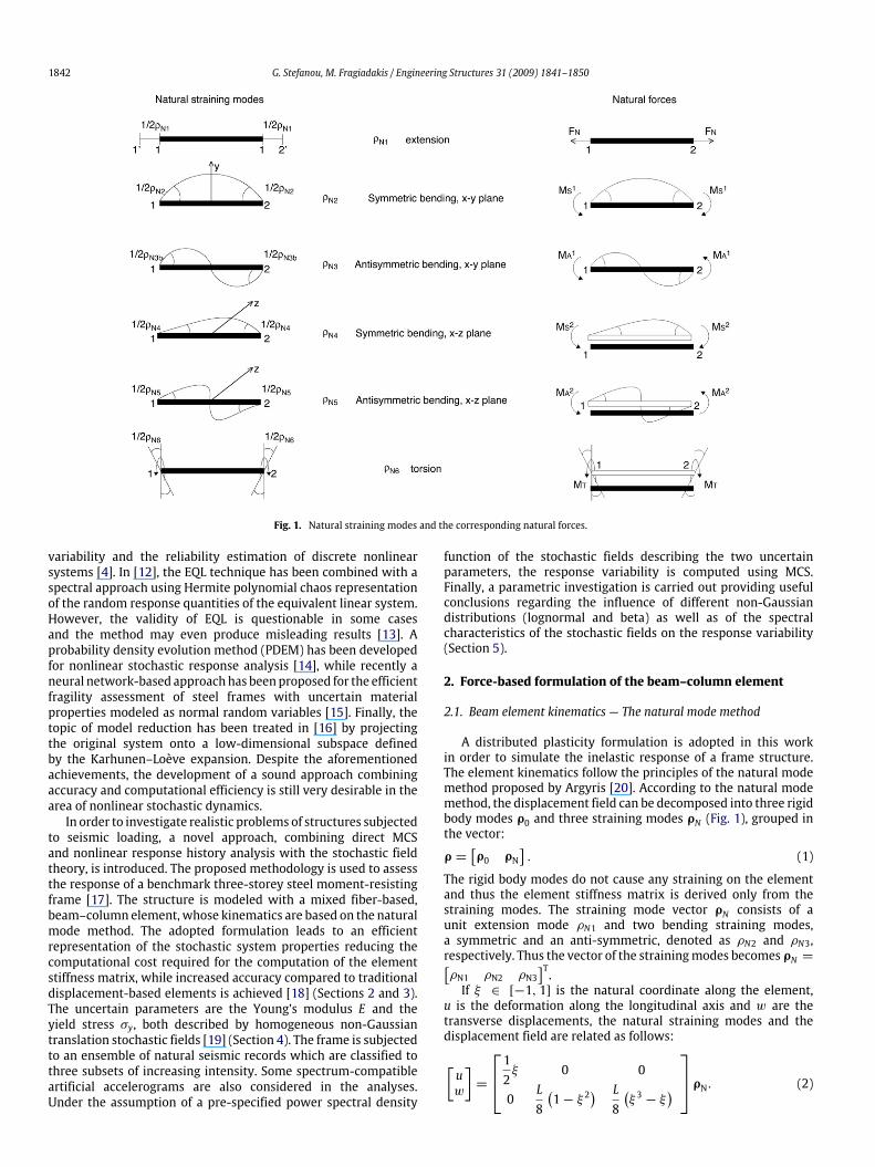
Fig. 1. Natural straining modes and the corresponding natural forces.

variability and the reliability estimation of discrete nonlinearsystems [4]. In [12], the EQL technique has been combined with aspectral approach using Hermite polynomial chaos representationof the random response quantities of the equivalent linear system.However, the validity of EQL is questionable in some casesand the method may even produce misleading results [13]. Aprobability density evolution method (PDEM) has been developedfor nonlinear stochastic response analysis [14], while recently aneural network-based approachhas beenproposed for the efficientfragility assessment of steel frames with uncertain materialproperties modeled as normal random variables [15]. Finally, thetopic of model reduction has been treated in [16] by projectingthe original system onto a low-dimensional subspace definedby the Karhunen–Loève expansion. Despite the aforementionedachievements, the development of a sound approach combiningaccuracy and computational efficiency is still very desirable in thearea of nonlinear stochastic dynamics.In order to investigate realistic problems of structures subjected

to seismic loading, a novel approach, combining direct MCSand nonlinear response history analysis with the stochastic fieldtheory, is introduced. The proposed methodology is used to assessthe response of a benchmark three-storey steel moment-resistingframe [17]. The structure is modeled with a mixed fiber-based,beam–column element, whose kinematics are based on the naturalmode method. The adopted formulation leads to an efficientrepresentation of the stochastic system properties reducing thecomputational cost required for the computation of the elementstiffness matrix, while increased accuracy compared to traditionaldisplacement-based elements is achieved [18] (Sections 2 and 3).The uncertain parameters are the Young’s modulus E and theyield stress σy, both described by homogeneous non-Gaussiantranslation stochastic fields [19] (Section 4). The frame is subjectedto an ensemble of natural seismic records which are classified tothree subsets of increasing intensity. Some spectrum-compatibleartificial accelerograms are also considered in the analyses.Under the assumption of a pre-specified power spectral density

function of the stochastic fields describing the two uncertainparameters, the response variability is computed using MCS.Finally, a parametric investigation is carried out providing usefulconclusions regarding the influence of different non-Gaussiandistributions (lognormal and beta) as well as of the spectralcharacteristics of the stochastic fields on the response variability(Section 5).

2. Force-based formulation of the beam–column element

2.1. Beam element kinematics — The natural mode method

A distributed plasticity formulation is adopted in this workin order to simulate the inelastic response of a frame structure.The element kinematics follow the principles of the natural modemethod proposed by Argyris [20]. According to the natural modemethod, the displacement field can be decomposed into three rigidbody modes ρ0 and three straining modes ρN (Fig. 1), grouped inthe vector:

ρ =[ρ0 ρN

]. (1)

The rigid body modes do not cause any straining on the elementand thus the element stiffness matrix is derived only from thestraining modes. The straining mode vector ρN consists of aunit extension mode ρN1 and two bending straining modes,a symmetric and an anti-symmetric, denoted as ρN2 and ρN3,respectively. Thus the vector of the strainingmodes becomes ρN =[ρN1 ρN2 ρN3

]T.If ξ ∈ [−1, 1] is the natural coordinate along the element,

u is the deformation along the longitudinal axis and w are thetransverse displacements, the natural straining modes and thedisplacement field are related as follows:

[uw

]=

12ξ 0 0

0L8

(1− ξ 2

) L8

(ξ 3 − ξ

)ρN. (2)

G. Stefanou, M. Fragiadakis / Engineering Structures 31 (2009) 1841–1850 1843

The above expression assumes a constant distribution of the axialdeformations, while for the second and third straining modesρN2 and ρN3, a quadratic and a cubic interpolation is adopted,respectively. Consequently, the axial strain εx is computed as:

εx =∂u∂x− y

∂2w

∂x2=1L(ρ N1 + yρN2 − 3yξρN3) . (3)

Furthermore, the relationship between the natural strainingmodes and the nodal displacements in the element local systemuel is obtained using simple algebraic transformations:ρN = aNuel (4)where aN is a transformation matrix.Similarly to the vector of the straining modes, the vector of

natural loads PN is defined. If ξ0 is an arbitrary section within theelement, the section forces Dsec are computed from the naturalloads with the interpolation matrix b, as follows:

Dsec (ξ0) = b (ξ0) PN ⇔[N0M0

]

=

[1 0 00 −1 ξ0

][PN1PN2PN3

](5)

where N0 and M0 are the axial force and the bending moment ofthe section ξ = ξ0, respectively. In addition, if dsec = [εx, κ]T isthe vector of section deformations that consists of the axial strainεx and the curvature κ , the deformation compatibility conditionimplies:

ρN =

∫ 1

−1bT(ξ)dsecdξ . (6)

2.2. Force-based element

Inelastic analysis of frame structures can be performed eitherwith a lumped or with a distributed plasticity formulation.Distributed plasticity elements are considered more accurateand, in general, are distinguished to displacement-based andto force-based elements. The latter approach has a number ofdistinct features over the former, especially if it is adopted in theframework of a mixed beam–column formulation [21]. The force-based formulation, also known as flexibility formulation, requires asingle beam–column element per member to simulate its materialnonlinear response, since it uses force interpolation functions.Consequently, the element equilibrium is always satisfied, whilecompatibility of deformations is satisfied by integrating the sectiondeformations to obtain the element deformations and the nodaldisplacements. In order to numerically calculate the stiffnessmatrix, a number of sections along the beam–column element arechosen, while every section is divided to a number of monitoringsections, known as fibers. Fibers are simply integration points of alow order quadrature at the section level and are used to evaluatethe section stiffness as follows:

Dsec = ksecdsec ⇔ Dsec =(∫A

∂σ

∂ε

[1 −y−y y2

]dA)dsec (7)

where y is the distance of a fiber from the neutral axis. If theresponse is linear elastic, the diagonal terms of the section stiffnessmatrix become equal to EA and EI, respectively, while the off-diagonal terms are zero. If the section flexibility matrix is fsec =k−1sec , the element flexibility matrix F = K

−1 is obtained as follows:

F = K−1 =∫ 1

−1bTk−1secbdξ =

∫ 1

−1bTfsecbdξ

=

NP∑i=1

wibT(ξi)fsec(ξi)b(ξi). (8)

The above equation implies that numerical integration is requiredin order to obtain the element flexibility matrix, where NP is thenumber of integration points along the element. In force-basedelements, the Gauss–Lobatto quadrature is preferred because itconsiders as sections of integration the beam ends where thebending moment is maximum (provided that no other elementloads are present). This integration scheme requires at least threeintegration sections, while typically four to six sections are chosen.In a flexibility-based element the calculation of the natural

element forces is performed iteratively for each element. Thefirst step of the iterative procedure is to determine the vector ofthe natural forces. Then using force interpolation functions, thesection forces are obtained and subsequently they are correctedaccording to the constitutive law. From the corrected forces thesection deformations are obtained (Eq. (7)) and are then integratedaccording to Eq. (6) to obtain the residual natural modes. Theiterative process in the element level is terminatedwhen an energyconvergence criterion is satisfied.

3. Stochastic finite element analysis

In the context of stochastic finite element analysis, theuncertain system properties are usually represented by stochasticfields [22]. The statistical properties of these fields are based eitheron experimental measurements or, when no experimental resultsare available, on an assumed variation. In this paper, the Young’smodulus E and the yield stressσy of the structure are assumed to bedescribed by two uncorrelated 1D-1V homogeneous non-Gaussianstochastic fields:E (x) = E0 [1+ f1(x)] (9)σy (x) = σ y0 [1 + f2(x)] (10)where E0 is themean value of the Young’smodulus, σy0 is themeanvalue of the yield stress of thematerial and f1(x), f2(x) are two zero-mean non-Gaussian homogeneous stochastic fields correspondingto the variability of the Young’s modulus and the yield stress,respectively.As the entries of the element flexibility matrix F of Eq. (8)

are nonlinear functions of the uncertain material properties, aclosed form expression for the stochastic flexibility matrix is notpossible to be established. However, the analytical expression ofthe stochastic section stiffness matrix ksec with stochastic materialproperties based on Eqs. (9) and (10) is derived below. The integralof Eq. (7) is calculated through summation over every fiber leadingto:

ksec =nfib∑i=1

[EiAi −EiAiyi−EiAiyi EiAiy2i

](11)

where nfib is the number of fibers in the section, Ei is the tangentmodulus of fiber i, which depends on the current strain value of thefiber and Ai is the fiber area. Having in mind the definition of ksecin Eq. (7) and combining Eqs. (9), (11), the following expression isobtained for the stochastic section stiffness matrix:

ksec = k(0)sec + f1(x)k(0)sec (12)

where k(0)sec is the mean value of ksec obtained from Eq. (11) bysubstituting the mean value of the tangent Young’s modulus E(0)i .The tangent modulus of the fibers is random, since it depends onthe yield stress value which according to Eq. (10) is also random.Thus ksec is a stochastic matrix that has the same probabilitydistribution as f1(x) due to Eq. (12), provided that none of thesection fibers has yielded, i.e. the yield stress has not beenexceeded. Once the fibers start to yield, the section stiffnessproperties are also affected by f2(x). The stochastic flexibilitymatrix of the beam–column element is calculated numericallyusing its deterministic formulation given in Eq. (8) and thestochastic stiffness.

1844 G. Stefanou, M. Fragiadakis / Engineering Structures 31 (2009) 1841–1850

Fig. 2. The three-storey LA3 steel frame.

4. Simulation of non-Gaussian system properties

The material properties of the structural problems examined,are assumed to be non-Gaussian. The problem of simulating non-Gaussian stochastic processes and fields has recently receivedconsiderable attention in the field of stochastic mechanics. Thisis due to the fact that several quantities arising in practicalengineering problems (e.g. material and geometric properties ofstructural systems, soil properties, wind loads, waves, etc) areusually found to exhibit non-Gaussian probabilistic characteristics.Since all the joint multi-dimensional density functions are

needed to fully characterize a non-Gaussian stochastic field,a number of studies has been focused on producing a morerealistic definition of a non-Gaussian sample function from asimple transformation of an underlying Gaussian field with knownsecond-order statistics. Thus, if g(x) is a homogeneous zero-meanGaussian field with unit variance and spectral density function(SDF) Sgg (κ) (or equivalently autocorrelation function Rgg (ξ )),a homogeneous non-Gaussian stochastic field f (x) with powerspectrum STff (κ) is defined as:

f (x) = F−1 · Φ[g(x)] (13)

whereΦ is the standard Gaussian cumulative distribution functionand F is the non-Gaussian marginal cumulative distributionfunction (CDF) of f (x). The transform F−1 · Φ is a memory-less translation since the value of f (x) at an arbitrary pointx depends on the value of g(x) at the same point only andthe resulting non-Gaussian field is called a translation field [19].Translation fields have a number of useful properties such asthe analytical calculation of crossing rates and extreme valuedistributions. Recently, it has been shown that the (stationary)stochastic response of a geometrically nonlinear cantilever beamcan be accurately calibrated using translation processes. The peakdynamic response distribution of the beamhas also been efficientlyestimated in this context [23]. Some algorithms extending thetranslation field concept and leading to the generation of non-Gaussian fields having the prescribed F and STff (κ), can be foundin [24,25].In the present work, Eq. (13) is used for the generation

of non-Gaussian translation sample functions representing theuncertain material properties. Sample functions of the underlyingGaussian field g(x) are generated using the spectral representationmethod [26]. The SDF Sgg (κ) of g(x) used in the numerical exampleis assumed to correspond to an autocorrelation function of squareexponential type and is given by:

Sgg(κ) =σ 2g b

2√πexp

(−b2κ2

4

)(14)

where σg is the standard deviation of the stochastic field and bdenotes the parameter that influences the shape of the spectrumand is proportional to the correlation length of the stochastic fieldalong the x-axis. The SDF of the translation field obtained fromEq. (13) will be slightly different from Sgg (κ).Using the procedure described in this section, a large number

NSAMP of non-Gaussian sample functions are produced, leadingto the generation of a set of stochastic stiffness matrices. Theassociated structural problem is solved NSAMP times and theresponse variability can finally be calculated by obtaining theresponse statistics of the NSAMP simulations.

5. Numerical examples

5.1. Structural model and earthquake loading

A numerical implementation of the above described methodol-ogy is demonstrated with the three-storey steel moment-resistingframe shown in Fig. 2. The frame has been designed for a Los An-geles site, following the 1997 NEHRP (National Earthquake HazardReduction Program) provisions in the framework of the SAC/FEMAprogram [27]. The dynamic response of the building is dominatedby the fundamental mode which has a period value equal to T1 =1.02 s when the mean value of the modulus of elasticity is used.All response history analyses were performed using a force-based,beam–column fiber element with five integration sections imple-mented on a general purpose finite element program [28]. Geo-metric nonlinearities were not considered in the analysis. Rayleighdamping is used to obtain a damping ratio of 2% for the first andthe fourth mode. The material law considered is bilinear with purekinematic hardening, where the properties of each integration sec-tion differ according to the stochastic fields of Eqs. (9) and (10). Theframe section properties belong to five groups: two for the columns(interior and exterior), and three for the beams (one for eachstorey). The gravity loading applied is 32.22 kN/m (2.208 kip/ft)for the first two stories and 28.76 kN/m (1.974 kip/ft) for the topstorey. These values are used also to obtain the nodal masses re-sulting in a lumped mass matrix.For the nonlinear dynamic procedure, three sets of five strong

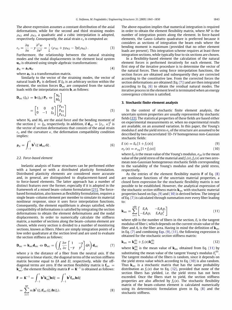
ground motion records were used (Table 1). As can be seen fromthe response spectra of Fig. 3, the three sets correspond to threelevels of increasing hazard: low, medium and high. Although thepredominant frequencies of the records lie at period values lessthan the fundamental elastic period of the frame, it is clear thatfor many of the records the amplification at the vicinity of 1.0 s israther significant. The records chosen differ in terms of amplitude,frequency content, duration, etc and therefore this variabilityis expected to be transferred to the statistics of the analysis,producing significant record-to-record variability. The records of

G. Stefanou, M. Fragiadakis / Engineering Structures 31 (2009) 1841–1850 1845

Fig. 3. Response Spectra of the 15 ground motion records of Table 1.

Table 1The ground motion records used.

ID (level) Earthquake Station ϕ0a Mwb Rc Soild PGA

1 (1/1) Imperial Valley, 1979 Plaster City 045 6.5 31.7 C, D 0.0422 (2/1) Imperial Valley, 1979 Plaster City 135 6.5 31.7 C, D 0.0573 (3/1) Imperial Valley, 1979 Westmoreland Fire Station 180 6.5 15.1 C, D 0.114 (4/1) Imperial Valley, 1979 Westmoreland Fire Station 090 6.5 15.1 C, D 0.0745 (5/1) Imperial Valley, 1979 Compuertas 285 6.5 32.6 C, D 0.1476 (1/2) Northridge, 1994 LA, Baldwin Hills 090 6.7 31.3 B, B 0.2397 (2/2) Imperial Valley, 1979 Plaster City 090 6.5 31.7 C, D 0.0578 (3/2) Loma Prieta, 1989 Sunnyvale Colton Ave 270 6.9 28.8 C, D 0.2079 (4/2) Superstition Hills, 1987 Wildlife Liquefaction Array 090 6.7 24.4 C, D 0.1810 (5/2) Loma Prieta, 1989 Sunnyvale Colton Ave 360 6.9 28.8 C, D 0.20911(1/3) Superstition Hills, 1987 Wildlife Liquefaction Array 360 6.7 24.4 C, D 0.212 (2/3) Northridge, 1994 LA, Hollywood Storage FF 360 6.7 25.5 C, D 0.35813 (3/3) Loma Prieta, 1989 Hollister South & Pine 000 6.9 28.8 –, D 0.37114 (4/3) Loma Prieta, 1989 WAHO 000 6.9 16.9 –, D 0.37015 (5/3) Loma Prieta, 1989 WAHO 090 6.9 16.9 –, D 0.638a Component.b Moment magnitude.c Closest distance to fault rupture.d USGS, Geomatrix soil class.

Table 2Range of definition and shape parameters of lognormal and beta distributions.

Lower bound Upper bound Shape parameters

Lognormal −1 +∞ – –L-beta −0.13 0.26 p = 0.8 q = 1.6

Table 1 are used as input for the analysis in order to compute themean response quantities and the dispersion for the three intensitylevels.Moreover, in order to examine the effect of stochastic

earthquake loading on the response variability, one thousandspectrum-compatible accelerograms are generated for everyintensity level (compatible with natural records 1/1, 4/2 and1/3, respectively) using the SIMQKE program by Gasparini and

Vanmarcke [29]. These natural records have been selected becausethey lead to the largest response variability for each intensity levelas will be shown in subsequent sections.

5.2. Structural response variability

The spatial variability in Young’s modulus and yield stress ofthe frame is described by two uncorrelated 1D-1V homogeneousnon-Gaussian translation stochastic fields with zero mean andcoefficient of variation equal to 0.10. Shifted lognormal and L-beta distributions are assumed for the two stochastic fields.The parameters of these distributions are listed in Table 2. Theskewness of the lognormal distribution is equal to 0.30 while theskewness of the L-beta distribution is 0.59. The representativeresponse quantity whose statistics are monitored is the maximum

1846 G. Stefanou, M. Fragiadakis / Engineering Structures 31 (2009) 1841–1850

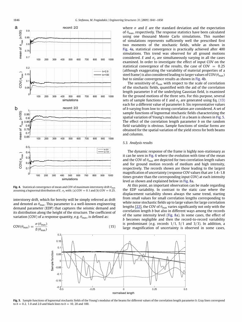
Fig. 4. Statistical convergence of mean and COV of maximum interstorey drift θmaxassuming a lognormal distribution of E, σy with: (a) COV = 0.1 and (b) COV = 0.25.

interstorey drift, which for brevity will be simply referred as driftand denoted as θmax. This parameter is a well-known engineeringdemand parameter (EDP) that captures the seismic demand andits distribution along the height of the structure. The coefficient ofvariation (COV) of a response quantity, e.g. θmax, is defined as:

COV(θmax) =σ(θmax)

E(θmax)(15)

where σ and E are the standard deviation and the expectationof θmax, respectively. The response statistics have been calculatedusing one thousand Monte Carlo simulations. This numberof simulations represents sufficiently well the prescribed firsttwo moments of the stochastic fields, while as shown inFig. 4a, statistical convergence is practically achieved after 400simulations. This trend was observed for all ground motionsconsidered. E and σy are simultaneously varying in all the casesexamined. In order to investigate the effect of input COV on thestatistical convergence of the results, the case of COV = 0.25(although exaggerating the variability of material properties of asteel frame) is also considered leading to larger values of COV(θmax)but to similar convergence results as shown in Fig. 4b.The sensitivity of θmax with respect to the scale of correlation

of the stochastic fields, quantified with the aid of the correlationlength parameter b of the underlying Gaussian field, is examinedfor the ground motions of the three sets. For this purpose, severalsets of sample functions of E and σy are generated using Eq. (13)each for a different value of parameter b. Six representative valuesof b varying from low to strong correlation are considered. A set ofsample functions of lognormal stochastic fields characterizing thespatial variation of Young’s modulus E in a beam is shown in Fig. 5.The effect of the correlation length parameter b on the randomfield variability is obvious. Sample functions of similar forms areobtained for the spatial variation of the yield stress for both beamsand columns.

5.3. Analysis results

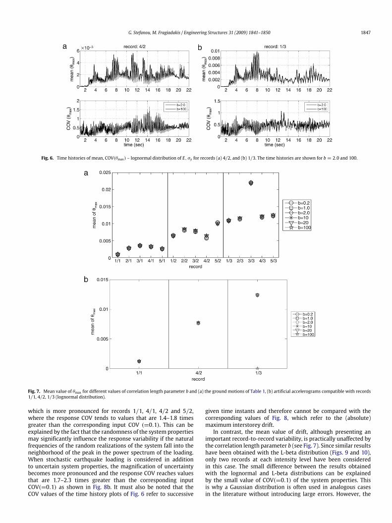
The dynamic response of the frame is highly non-stationary asit can be seen in Fig. 6 where the evolution with time of the meanand the COV of θmax are depicted for two correlation length valuesand for ground motion records of medium and high intensity,respectively. The records shown are those leading to the largestmagnification of uncertainty (response COV values that are 1.4–1.8times greater than the corresponding input COV) at each intensitylevel as shown and explained below in Fig. 8a.At this point, an important observation can be made regarding

the EDP variability. In contrast to the static case where thedisplacement variability shows always the same trend, startingfrom small values for small correlation lengths corresponding towhite noise stochastic fields up to large values for large correlationlengths [22], the COV of θmax varies significantly not only with thecorrelation length b but also in different ways among the recordsof the same intensity level (Fig. 8a). In some cases, the effect ofb becomes negligible and then the record-to-record variabilityis predominant (e.g. records 1/1, 5/1 and 3/3). In addition, alarge magnification of uncertainty is observed in some cases,

Fig. 5. Sample functions of lognormal stochastic fields of the Young’s modulus of the beams for different values of the correlation length parameter b. Gray lines correspondto b = 0.2, 1.0 and 2.0 and black lines to b = 10, 20 and 100.

G. Stefanou, M. Fragiadakis / Engineering Structures 31 (2009) 1841–1850 1847

Fig. 6. Time histories of mean, COV(θmax) – lognormal distribution of E, σy for records (a) 4/2, and (b) 1/3. The time histories are shown for b = 2.0 and 100.

Fig. 7. Mean value of θmax for different values of correlation length parameter b and (a) the ground motions of Table 1, (b) artificial accelerograms compatible with records1/1, 4/2, 1/3 (lognormal distribution).

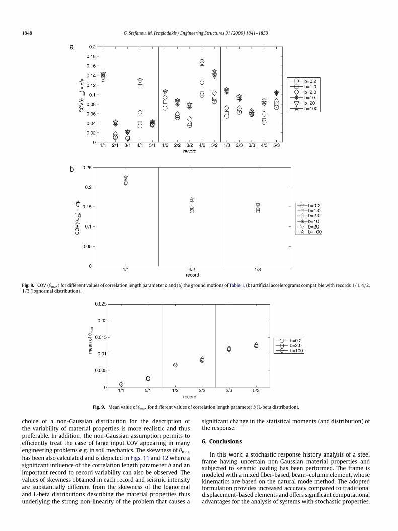
which is more pronounced for records 1/1, 4/1, 4/2 and 5/2,where the response COV tends to values that are 1.4–1.8 timesgreater than the corresponding input COV (=0.1). This can beexplained by the fact that the randomness of the system propertiesmay significantly influence the response variability if the naturalfrequencies of the random realizations of the system fall into theneighborhood of the peak in the power spectrum of the loading.When stochastic earthquake loading is considered in additionto uncertain system properties, the magnification of uncertaintybecomes more pronounced and the response COV reaches valuesthat are 1.7–2.3 times greater than the corresponding inputCOV(=0.1) as shown in Fig. 8b. It must also be noted that theCOV values of the time history plots of Fig. 6 refer to successive

given time instants and therefore cannot be compared with thecorresponding values of Fig. 8, which refer to the (absolute)maximum interstorey drift.In contrast, the mean value of drift, although presenting an

important record-to-record variability, is practically unaffected bythe correlation length parameter b (see Fig. 7). Since similar resultshave been obtained with the L-beta distribution (Figs. 9 and 10),only two records at each intensity level have been consideredin this case. The small difference between the results obtainedwith the lognormal and L-beta distributions can be explainedby the small value of COV(=0.1) of the system properties. Thisis why a Gaussian distribution is often used in analogous casesin the literature without introducing large errors. However, the

1848 G. Stefanou, M. Fragiadakis / Engineering Structures 31 (2009) 1841–1850

Fig. 8. COV (θmax) for different values of correlation length parameter b and (a) the groundmotions of Table 1, (b) artificial accelerograms compatible with records 1/1, 4/2,1/3 (lognormal distribution).

Fig. 9. Mean value of θmax for different values of correlation length parameter b (L-beta distribution).

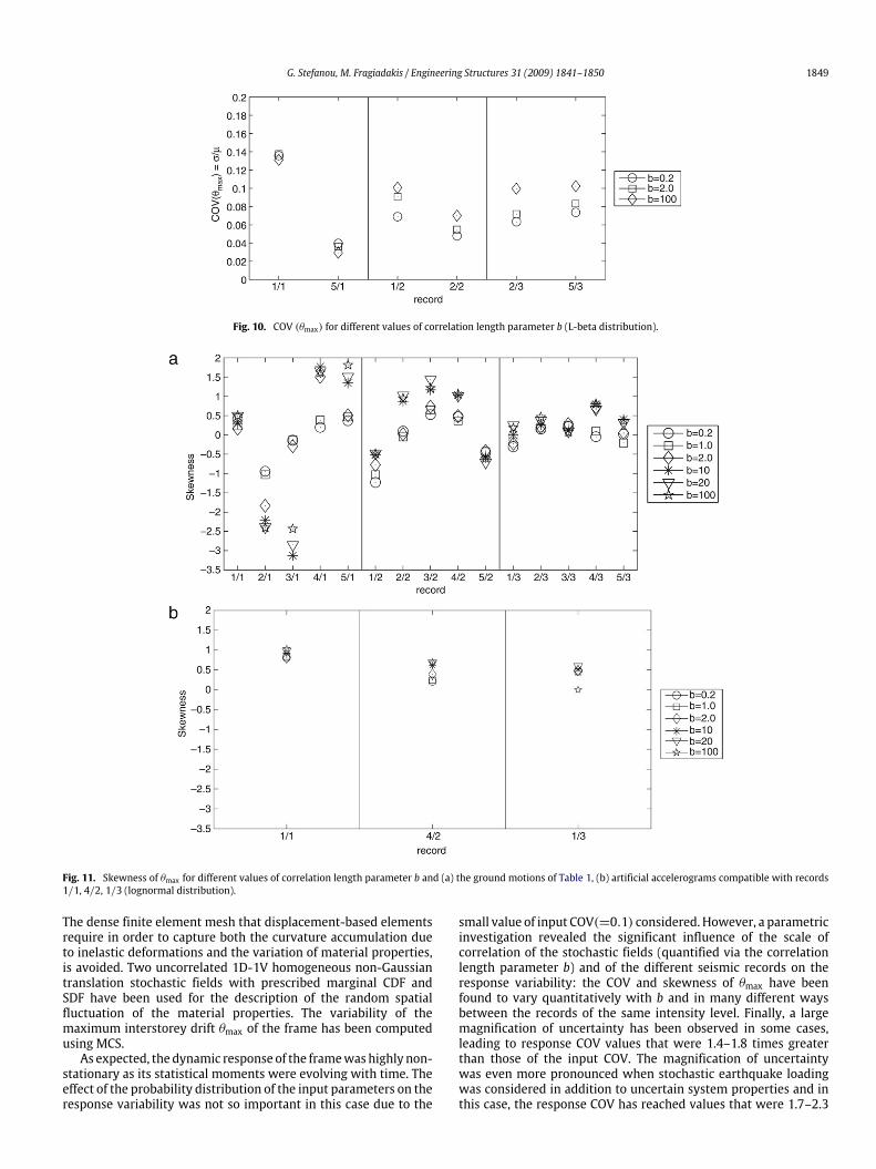
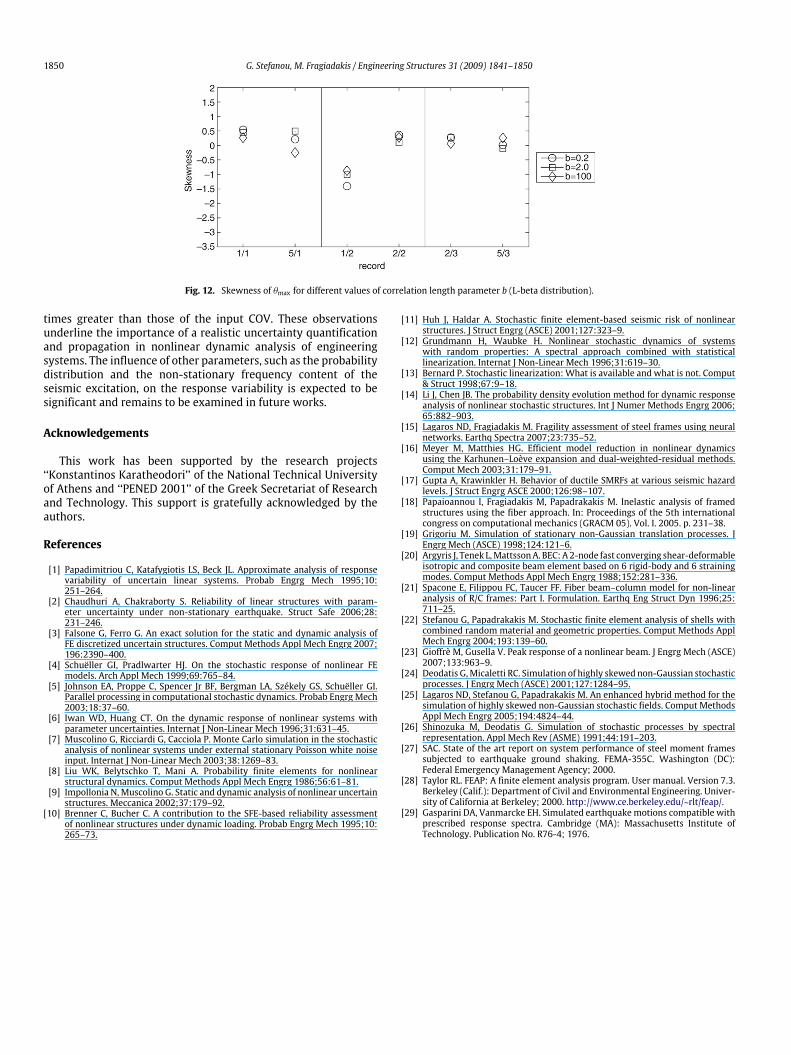
choice of a non-Gaussian distribution for the description ofthe variability of material properties is more realistic and thuspreferable. In addition, the non-Gaussian assumption permits toefficiently treat the case of large input COV appearing in manyengineering problems e.g. in soil mechanics. The skewness of θmaxhas been also calculated and is depicted in Figs. 11 and 12 where asignificant influence of the correlation length parameter b and animportant record-to-record variability can also be observed. Thevalues of skewness obtained in each record and seismic intensityare substantially different from the skewness of the lognormaland L-beta distributions describing the material properties thusunderlying the strong non-linearity of the problem that causes a

significant change in the statistical moments (and distribution) ofthe response.

6. Conclusions

In this work, a stochastic response history analysis of a steelframe having uncertain non-Gaussian material properties andsubjected to seismic loading has been performed. The frame ismodeled with a mixed fiber-based, beam–column element, whosekinematics are based on the natural mode method. The adoptedformulation provides increased accuracy compared to traditionaldisplacement-based elements and offers significant computationaladvantages for the analysis of systems with stochastic properties.

G. Stefanou, M. Fragiadakis / Engineering Structures 31 (2009) 1841–1850 1849

Fig. 10. COV (θmax) for different values of correlation length parameter b (L-beta distribution).

Fig. 11. Skewness of θmax for different values of correlation length parameter b and (a) the ground motions of Table 1, (b) artificial accelerograms compatible with records1/1, 4/2, 1/3 (lognormal distribution).

The dense finite element mesh that displacement-based elementsrequire in order to capture both the curvature accumulation dueto inelastic deformations and the variation of material properties,is avoided. Two uncorrelated 1D-1V homogeneous non-Gaussiantranslation stochastic fields with prescribed marginal CDF andSDF have been used for the description of the random spatialfluctuation of the material properties. The variability of themaximum interstorey drift θmax of the frame has been computedusing MCS.As expected, the dynamic response of the framewashighly non-

stationary as its statistical moments were evolving with time. Theeffect of the probability distribution of the input parameters on theresponse variability was not so important in this case due to the

small value of input COV(=0.1) considered. However, a parametricinvestigation revealed the significant influence of the scale ofcorrelation of the stochastic fields (quantified via the correlationlength parameter b) and of the different seismic records on theresponse variability: the COV and skewness of θmax have beenfound to vary quantitatively with b and in many different waysbetween the records of the same intensity level. Finally, a largemagnification of uncertainty has been observed in some cases,leading to response COV values that were 1.4–1.8 times greaterthan those of the input COV. The magnification of uncertaintywas even more pronounced when stochastic earthquake loadingwas considered in addition to uncertain system properties and inthis case, the response COV has reached values that were 1.7–2.3

1850 G. Stefanou, M. Fragiadakis / Engineering Structures 31 (2009) 1841–1850

Fig. 12. Skewness of θmax for different values of correlation length parameter b (L-beta distribution).

times greater than those of the input COV. These observationsunderline the importance of a realistic uncertainty quantificationand propagation in nonlinear dynamic analysis of engineeringsystems. The influence of other parameters, such as the probabilitydistribution and the non-stationary frequency content of theseismic excitation, on the response variability is expected to besignificant and remains to be examined in future works.

Acknowledgements

This work has been supported by the research projects‘‘Konstantinos Karatheodori’’ of the National Technical Universityof Athens and ‘‘PENED 2001’’ of the Greek Secretariat of Researchand Technology. This support is gratefully acknowledged by theauthors.

References

[1] Papadimitriou C, Katafygiotis LS, Beck JL. Approximate analysis of responsevariability of uncertain linear systems. Probab Engrg Mech 1995;10:251–264.

[2] Chaudhuri A, Chakraborty S. Reliability of linear structures with param-eter uncertainty under non-stationary earthquake. Struct Safe 2006;28:231–246.

[3] Falsone G, Ferro G. An exact solution for the static and dynamic analysis ofFE discretized uncertain structures. Comput Methods Appl Mech Engrg 2007;196:2390–400.

[4] Schuëller GI, Pradlwarter HJ. On the stochastic response of nonlinear FEmodels. Arch Appl Mech 1999;69:765–84.

[5] Johnson EA, Proppe C, Spencer Jr BF, Bergman LA, Székely GS, Schuëller GI.Parallel processing in computational stochastic dynamics. Probab Engrg Mech2003;18:37–60.

[6] Iwan WD, Huang CT. On the dynamic response of nonlinear systems withparameter uncertainties. Internat J Non-Linear Mech 1996;31:631–45.

[7] Muscolino G, Ricciardi G, Cacciola P. Monte Carlo simulation in the stochasticanalysis of nonlinear systems under external stationary Poisson white noiseinput. Internat J Non-Linear Mech 2003;38:1269–83.

[8] Liu WK, Belytschko T, Mani A. Probability finite elements for nonlinearstructural dynamics. Comput Methods Appl Mech Engrg 1986;56:61–81.

[9] Impollonia N, Muscolino G. Static and dynamic analysis of nonlinear uncertainstructures. Meccanica 2002;37:179–92.

[10] Brenner C, Bucher C. A contribution to the SFE-based reliability assessmentof nonlinear structures under dynamic loading. Probab Engrg Mech 1995;10:265–73.

[11] Huh J, Haldar A. Stochastic finite element-based seismic risk of nonlinearstructures. J Struct Engrg (ASCE) 2001;127:323–9.

[12] Grundmann H, Waubke H. Nonlinear stochastic dynamics of systemswith random properties: A spectral approach combined with statisticallinearization. Internat J Non-Linear Mech 1996;31:619–30.

[13] Bernard P. Stochastic linearization: What is available and what is not. Comput& Struct 1998;67:9–18.

[14] Li J, Chen JB. The probability density evolution method for dynamic responseanalysis of nonlinear stochastic structures. Int J Numer Methods Engrg 2006;65:882–903.

[15] Lagaros ND, Fragiadakis M. Fragility assessment of steel frames using neuralnetworks. Earthq Spectra 2007;23:735–52.

[16] Meyer M, Matthies HG. Efficient model reduction in nonlinear dynamicsusing the Karhunen–Loève expansion and dual-weighted-residual methods.Comput Mech 2003;31:179–91.

[17] Gupta A, Krawinkler H. Behavior of ductile SMRFs at various seismic hazardlevels. J Struct Engrg ASCE 2000;126:98–107.

[18] Papaioannou I, Fragiadakis M, Papadrakakis M. Inelastic analysis of framedstructures using the fiber approach. In: Proceedings of the 5th internationalcongress on computational mechanics (GRACM 05). Vol. I. 2005. p. 231–38.

[19] Grigoriu M. Simulation of stationary non-Gaussian translation processes. JEngrg Mech (ASCE) 1998;124:121–6.

[20] Argyris J, Tenek L,MattssonA. BEC: A2-node fast converging shear-deformableisotropic and composite beam element based on 6 rigid-body and 6 strainingmodes. Comput Methods Appl Mech Engrg 1988;152:281–336.

[21] Spacone E, Filippou FC, Taucer FF. Fiber beam–column model for non-linearanalysis of R/C frames: Part I. Formulation. Earthq Eng Struct Dyn 1996;25:711–25.

[22] Stefanou G, Papadrakakis M. Stochastic finite element analysis of shells withcombined random material and geometric properties. Comput Methods ApplMech Engrg 2004;193:139–60.

[23] Gioffrè M, Gusella V. Peak response of a nonlinear beam. J Engrg Mech (ASCE)2007;133:963–9.

[24] Deodatis G,Micaletti RC. Simulation of highly skewed non-Gaussian stochasticprocesses. J Engrg Mech (ASCE) 2001;127:1284–95.

[25] Lagaros ND, Stefanou G, Papadrakakis M. An enhanced hybrid method for thesimulation of highly skewed non-Gaussian stochastic fields. Comput MethodsAppl Mech Engrg 2005;194:4824–44.

[26] Shinozuka M, Deodatis G. Simulation of stochastic processes by spectralrepresentation. Appl Mech Rev (ASME) 1991;44:191–203.

[27] SAC. State of the art report on system performance of steel moment framessubjected to earthquake ground shaking. FEMA-355C. Washington (DC):Federal Emergency Management Agency; 2000.

[28] Taylor RL. FEAP: A finite element analysis program. User manual. Version 7.3.Berkeley (Calif.): Department of Civil and Environmental Engineering. Univer-sity of California at Berkeley; 2000. http://www.ce.berkeley.edu/~rlt/feap/.

[29] Gasparini DA, Vanmarcke EH. Simulated earthquakemotions compatible withprescribed response spectra. Cambridge (MA): Massachusetts Institute ofTechnology. Publication No. R76-4; 1976.