Stationarity and structural breaks — evidence from classical and Bayesian approaches

Ž .Economic Modelling 18 2001 503�524

Stationarity and structural breaks �evidence from classical and Bayesian

approaches

Antonio E. Noriegaa,�, Enrique de Albab,1

a Department of Econometrics, School of Economics, Uni�ersidad de Guanajuato,36000 Guanajuato, Mexico

bDi�ision of Actuarial Science, Statistics and Mathematics, Instituto Tecnologico Autonomo de´ ´( )Mexico ITAM , Mexico, Mexico´

Accepted 21 June 2000

Abstract

The purpose of this paper is to analyze and compare the results of applying classical andBayesian methods to testing for a unit root in time series with a single endogenousstructural break. We utilize a data set of macroeconomic time series for the Mexicaneconomy similar to the Nelson�Plosser one. Under both approaches, we make use ofinnovational outlier models allowing for an unknown break in the trend function. Classicalinference relies on bootstrapped critical values, in order to make inference comparable tothe finite sample Bayesian one. Results from both approaches are discussed and compared.� 2001 Elsevier Science B.V. All rights reserved.

JEL classifications: C11; C12; C13; C15; C22

Keywords: Difference stationary; Structural break; Classical and Bayesian analyses; Macroeconomictime series; Resampling methods

� Corresponding author. Tel.: �52-473-20105; fax: �52-473-20105.Ž . Ž .E-mail addresses: [email protected] A.E. Noriega , [email protected] E. de Alba .

1Rio Hondo 1, Tizapan, San Angel, 0100, Mexico, D.F. Tel.: �52-5628-4080. Supported by Associacion´ ´Mexicana de Cultura, A.C., Rio Hondo 1, Mexico, D.F.´

0264-9993�01�$ - see front matter � 2001 Elsevier Science B.V. All rights reserved.Ž .PII: S 0 2 6 4 - 9 9 9 3 0 0 0 0 0 5 0 - X

( )A.E. Noriega, E. de Alba � Economic Modelling 18 2001 503�524504

1. Introduction

Ž .Perron 1989 demonstrated the importance of correctly specifying the trendfunction when testing for unit roots. The basic idea is that ‘fixed’ linear time trendsare an extremely simple parameterization representing secular or long-run move-ments in economic time series. Models were proposed which take into account theoccurrence of ‘structural breaks’ due to wars, economic crises, changes in institu-tional arrangements, etc., by the inclusion of dummy variables in the trend

Ž .function. Perron 1992, 1997 presents extensive empirical evidence on the applica-tion of these methods to the Nelson�Plosser data set as well as to internationaldata sets on production variables. In general, the empirical findings seem tosuggest that rejection of the unit root hypothesis heavily depends on the specifica-tion of the long-run deterministic trend function.

The problem has also been extensively analyzed within a Bayesian frameworkŽ .Sims, 1988; Phillips, 1991; Lubrano, 1995; Tsurumi and Wago, 1996 . Zivot and

Ž .Phillips 1994 analyzed the Nelson�Plosser data using Bayesian methods allowingfor one endogenous break in the trend, with the break occurring near 1929 formost of the series. Before they allow for a break in the trend their empirical results

Ž .are in general agreement with those obtained in Phillips 1991 , where most seriesseem to show evidence of a stochastic trend. Using a flat, non-informative, priordistribution, as well as his approximate Jeffreys’ prior, Phillips conducted a Bayesiananalysis of the Nelson�Plosser data. With the flat prior he found insufficientevidence in favor of the stochastic trend for most series. With an approximateJeffreys’ prior he found more support for the unit root in three out of the 14 series.Furthermore, Bayesian methods support the point of view that the Nelson�Plosserdata can be better modelled when allowance is made for one break in the trend.

Ž .Stock 1994 discusses four motivations for testing univariate non-stationarity ineconomic time series. The purpose of this paper is related to two of thosemotivations: to identify data description models and to analyze the univariatebehaviour of the time series in order to guide subsequent multivariate modeling.To this end, we apply techniques from both classical and Bayesian approaches, tomodel some of the more important macroeconomic variables for the Mexicaneconomy, allowing for the presence of a structural break in the trend function.

Ž .Maddala and Kim 1996 present a selective survey of the literature on structuralbreaks and on tests for unit roots under structural breaks, under both the classicaland Bayesian approaches. However, to the best of our knowledge, there is noevidence in the literature of simultaneously applying both approaches to the issueof testing for a unit root while endogenously estimating a structural break. Two

Ž .strong arguments discussed in Zivot and Phillips 1994 , call for the use of Bayesianmethods. First, the classical break point estimation procedure produces a pretest-

Žing bias in any subsequent inference the bias depending on the procedure.employed . The problem is that if the break point is not known, its location will be

Ž .determined by means of a test of hypothesis. Then, given the result of this firstŽ .test, a second test is carried out for the unit root. The statistical characteristics of

the second test are really dependent on the first one, but usually not taken into

( )A.E. Noriega, E. de Alba � Economic Modelling 18 2001 503�524 505

Ž .account see Poirier, 1995, p.519; Maddala and Kim, 1996, p.83 . Under a Bayesianapproach conditional inferences concerning the parameters of the model can becarried out by detecting the points with greatest probability of being a break intrend. In this problem, Bayesian inference on the break point is done by means of

Ž .the posterior probability distribution that each one of the points in the series isthe break point. The ‘probability of a unit root’ can then be determined, conditio-nal on a given break point. Marginal distributions can be used to carry outunconditional inferences. Second, the resulting limit theory under the classicalapproach is quite complicated and the finite sample distributions of the unit roottest statistics can be very different from their asymptotic counterparts. Under theBayesian approach, the distribution theory is valid in finite samples. In this paper,classical inference relies on bootstrapped critical values, in order to make inferencecomparable to the finite sample Bayesian one.2 Results from both approaches arediscussed and compared.

We believe that the double analysis done in this paper has several contributions.In the first place it provides a formal analysis of the existence of unit roots in theMexican macroeconomic time series that has not been done before under anyapproach. Another important point is the comparison of the two approaches.Those readers inclined to the classical approach can see that the results of thealternative analysis is not all that different, and vice versa. This may hopefullycontribute to a better mutual understanding of both schools of thought. It may alsoprovide some evidence of the robustness of either, or both, of the approaches,since they essentially support each other. Thus, for instance, if in the classical casethere is some concern as to how well the modelling approach works, or regardingthe extent of pre-test bias, the Bayesian results provide some assurance as to theirreliability. On the other hand if in the Bayesian approach there may be concern asto the consequences of using non-informative priors, our results support the wellknown fact that in this case they approach the classical ones. In either case anapplied econometrician hesitant as to which approach to follow may gain someinsight for his decision from this paper.

2. The data and motivation

The data set analyzed in this paper consists of annual observations on elevenmajor macroeconomic time series for Mexico, all starting around the first quarterof this century and ending in 1970. We do not use data beyond that year becausethere have been changes in the methodology used to construct the series. Thesecould be confounded with true breaks in the series. Some features of the data areworth noting. First, the great majority of the series shows an increasing trend,exceptions being Income�Velocity of Money and Real Wages, which are relatively

2 Ž . Ž .Perron 1997 reports critical values, both asymptotic and finite sample, for classical unit root testsallowing for an endogenous structural break. He notes that, when a data-dependent method is used to

Ž .select the AR order as in this paper , the asymptotic approximation is not as good. We found that ourresults are not affected if asymptotic critical values are used.


more stable. Second, all the production variables, M4, Public Federal In�estmentand the GDP Deflator seem to have had, a ‘break’ in their long term trend at thebeginning of the 1930s. Another apparent change occurs around 1950 for theWholesale Price Index, Nominal and Real Wages and Public Federal In�estment.

Ž .These apparent break dates coincide with the view of Solıs 1970 : ‘...we find in´Mexican economic history two periods clearly differentiated: a period withouteconomic growth, which spans the years 1910�1935, and a period of defined

� �economic growth, which starts in 1935 and continues until the present day 1970 ’Ž .p.86 . According to Solıs, the 1929 great crash did affect the levels of economic´activity in Mexico: in 1932 exports were one-third of what they had been in 1929,and the federal government’s income decreased 25% from 1930 to 1933. In orderto keep a balanced budget, public spending was reduced 25% during the period of1930�1932. By 1931, Mexico abandoned the Gold Standard and in 1933 there wasan 80% devaluation of the peso. The second apparent break in the early 1950s

Ž .marks the transition from a period of growth with inflation 1935�1956 to a periodŽ .of growth with price and exchange rate stability 1956�1970 , as documented by

Solıs. During the inflation period, he argues, changes in institutional arrangements´� such as greater mobility of production factors, an increase in the educational

level of the population and the strengthening of the private sector, were responsi-ble for the transition to a long period of growth with greater stability.

The heterogeneous behavior in the historical trends of many observedŽ .macroeconomic time series, has led to the now standard use of models allowing

Ž .three types of breaks in the trend function: a change of level called model 1 , aŽ . Žchange of both level and slope called model 2 , and a change of slope alone called

. Žmodel 3 . Examples of these ‘breaking trend’ models can be found in Perron 1989,.1993, 1997 . A further classification of these models reflects the response of the

Ž .trend function to the breaks. Perron 1997 considers two types of responses of thetrend function following the break. The first one models an instantaneous change

Ž .to the new trend function and is called the ‘Additive Outlier Model’ AOM . Thesecond allows a gradual path to the new trend function and is called the ‘Innova-

Ž .tional Outlier Model’ IOM . However, in the empirical applications below, weŽ .only use IO models to allow a change in level of trend alone called IOM1 , a

Ž .change in level and slope of trend called IOM2 , and a change in slope of trendŽ . Ž .alone called IOM3 , as in Zivot and Phillips 1994 , since the AO model is

somewhat restrictive because it specifies that the full impact of a shock to the trendŽ .is felt instantaneously. See also de Jong 1996 .

3. Models and procedures

3.1. Classical approach

Consider a situation in which interest centers on testing whether or not devia-tions from a broken trend, defined as follows, are stationary:

Ž .y � � � � t � � DT � z 1t t t


for t � 1, . . . ,T , where T is the sample size and z is an outlier-free time series, ortthe ‘noise’ model, defined as

Ž . Ž . Ž .C L z � B L e 2t t

� 4Here e is a sequence of independent identically distributed random variables,tŽ . Ž m. Ž . Ž n.C L � 1 � c L � �� c L and B L � 1 � b L � �� b L are poly-1 m 1 n

nomials in the lag operator L, and DT is a dummy variable allowing a change intŽ . Ž . Ž .the trend’s slope after the break, that is, DT � t � T l t � T , where l � is thet b b

indicator function and T is the unknown date of the break.bŽ .In the ‘innovational’ outlier model IOM , the dynamics of the transition to the

new trend mimic those of the innovations e ,3t

Ž .B LŽ . Ž .y � � � � t � � DU � � DT � z 3t t t tŽ .C L

where DU is a dummy variable allowing a change in the trend’s level after thetŽ . Ž .break, that is, DU � l t � T . In Eq. 3 the linear trend and the break dummiest b

are subtracted from the data, however, the dummy variables are affected by theŽ . Ž .Ž .same dynamics affecting e . Rearranging Eq. 3 we get A L y � � � � t �t t

� DU � � DT � e or,t t t

p Ž .y � c � bt � � DU � � DT � Ý a y � e 4t t t i�1 i t�i t

Ž . Ž .�1 Ž .where A L � B L C L represents an infinite order polynomial if movingaverage components are present. In practice, this infinite sum is approximated by a

Ž . � Žfinite sum in order to derive operational tests see Perron, 1993 . Also, c � � 1 �. p � Ž . p� � �Ý ia and b � � 1 � � , with � � Ý a . We can reparametrize Eq.1 i�1 i 1 1 i�1 i

Ž . Ž .4 as see Fuller, 1996, ch.10 :

k Ž . y � c � bt � � DU � � DT � � y � Ý � y � e 5t t t t�1 j�1 j�1 t�j t

where k � p � 1, � � � � 1, and � � �Ý p a , i � 2,3, . . . , p. From the results1 i j�i jŽ . Ž .of Said and Dickey 1984 we can interpret the sum in Eq. 5 as the autoregressive

Ž . Ž .approximation of the ARMA process given in Eq. 2 for the noise function. Eq. 5Ž .can then be used to test the null hypothesis of a unit root H :� � 0 against the0

alternative of stationary fluctuations around a trend with a break in both level andŽ .slope of trend Ha:� � 0 . For the case of a change in the trend’s level alone

Ž . Ž .IOM1 we make � � 0 in Eq. 5 , while for the case of a change in the trend’sŽ . Ž .slope alone IOM3 the model is again Eq. 5 but now with � � 0. These can be

written, respectively, as:

k Ž . y � c � bt � � DU � � y � Ý � y � e 6t t t�1 j�1 j�1 t�j t

k Ž . y � c � bt � � DT � � y � Ý � y � e 7t t t�1 j�1 j�1 t�j t

3The discussion is centered on the IOM2, since it encompasses the IOM1 and IOM3.


There is little indication in the literature on model selection procedures forchoosing among IO models. We use the following procedure to simultaneously

Ž .determine the break date, T , and the lag length, k both of which are unknown ,btogether with the type of IO model. This procedure is used with three differentcriteria to estimate the break point. The first one is called the Min t criterion and�

works as follows. We first fix an arbitrary maximum value for k, labeled k . Thenmaxwe estimate by OLS each of the IO models, 1, 2, and 3, over all possible values ofT , and choose, for each model, the break date for which the unit root is rejectedb

Ž . Ž .with highest probability. This occurs when the t-statistic on � in Eqs. 5 � 7 isŽ .minimized. The Akaike Information Criterion AIC is then calculated for each of

the three regressions corresponding to the estimated break dates. If the coefficienton the k �th lag is not significant for the model which yields the smallest AIC,max

Ž . Ž .then we estimate Eqs. 5 � 7 again, over all possible values of T with k � 1b maxlags of the differenced-dependent variable. Again, we choose that date of the breakfor which the unit root is rejected with the highest probability, and compute theAIC for the three regressions corresponding to the newly estimated break dates.Continuing in this fashion, we select the combination ‘model type�lag length’ which

Žcorresponds to the model which yields the smallest value of the AIC amongst the. Ž .three models and a corresponding significant lag called k , using a two-sidedsig

10% test based on the asymptotic normal distribution. Note that if there are noŽ .significant lags, then k � 0 which implies p � 1 . If this is the case, thesig

selection of the model follows simply from the lowest value of the AIC.4Ž .The t-statistic for testing the null hypothesis of a unit root, H :� � 0 in Eq. 50

Ž . Ž . Ž . Ž . Ž .IOM2 , Eq. 6 IOM1 or Eq. 7 IOM3 is the one that minimizes t over allapossible values of T given k :b sig

Ž . Ž . Ž .t i � Min t i ,T k , i � IOM1,IOM2,IOM3� � b , sigˆ ˆŽ .T � k�3,T�3b

Ž .An alternative procedure employed by Perron 1997 selects T as that periodbfor which the structural break is not rejected with the highest probability among all

Ž .possible break points. This occurs for model 1 when the absolute value of theŽ Ž ..t-statistic on the change of level t in Eq. 6 is maximized. For models 2 and 3ˆ��

Ž .this occurs when the absolute value of the t-statistic on the change of slope �t �� ˆŽ . Ž .in Eq. 5 or Eq. 7 , respectively � is maximized. We call these criteria Max t ˆ��

and Max t , respectively. Under these criteria, the AIC is again used to jointly�� ˆdetermine the combination model type�lag length. The t-statistic for testing the

Ž . Ž .null hypothesis of a unit root, H :� � 0 in Eq. 6 IOM1 , is defined as0

ˆŽ . Ž .t 1 � t 1,T ,k , 8ž /� �� b sigˆ ˆ

4 Ž . Ž .Diebold and Senhadji 1996 report the best-fitting regression for k � 2,3,4. In Rudebusch 1992 ,the order of the autoregressions is fixed to two, irrespective of whether a difference�stationary or a

Ž .trend�stationary model is estimated. Rudebusch 1993 uses AR orders four, six and eight.


ˆ ˆŽ . � Ž . �where T is such that t T � Max t 1,T ,k . The t-statistics forˆ ˆ ˆb �� b T � Žk�3,T�3. � b sigbŽ . Ž . Ž . Ž .testing the null hypothesis of a unit root in Eq. 5 IOM2 and Eq. 7 IOM3 are

analogously defined as

ˆŽ . Ž .t i � t i ,T ,k , 9ž /� �� b sigˆ ˆ

ˆ ˆŽ . � Ž . �where T is such that t T � Max t i,T ,k ,i � IOM2,IOM3.b �� b T � Žk�3,T�3. � b sigˆ ˆbŽ .As discussed in Perron 1997 a substantial increase in power can be gained if

the restriction of a specific direction of the change in the trend function is imposeda priori. For example, for the Price Index, there seems to be a decrease in the

ˆŽ .trend’s slope. So, the test for a unit root is carried out using t i where now T is�� bˆˆŽ . Ž . Ž .such that t T � Min t i,T ,k , i � IOM2,IOM3 instead of Eq.� b T � Žk�3,T�3. � b sigˆ ˆb

Ž . Ž .9 . A similar argument applies to Eq. 8 .Ž . Ž .The third criterion we use, discussed in Bai 1997a,b ; Bai and Perron 1998a,b

chooses, among all possible break dates, the one which yields the smallest residualŽ . Ž .sum of squares from Eqs. 5 � 7 . Again, this is done for all values of k k .max

Under these criteria, the AIC is again used to determine the combination modeltype�lag length. We call this the min RSS criterion.

To carry out hypothesis testing regarding the presence of a unit root wecompute, by simulation, the sampling distributions of the t-statistic on the autore-

Ž . Ž .gressive parameter in Eqs. 5 � 7 under two competing hypotheses: a BreakingŽ .Trend�Stationary model with one break BTS, the alternative hypothesis , and a

Ž . Ž . Ž .Difference�Stationary model without break DS, the null hypothesis . Eqs. 5 � 7correspond to the IOM2, IOM1 and IOM3, respectively, under the BTS alterna-

Ž . Ž .tive. The Data�Generation Process DGP for these models the DS null is,

k Ž . y � Ý a y � e 10t i�1 i t�i t

We now present the resampling methodology used in the empirical applicationsfor the case of the IOM2 under the Min t criterion:5

�

Ž .1. Eq. 5 is run by OLS, and the estimated parameters are the ones whichcorrespond to using the Min t criterion, implying that estimates of T and k� bˆare also obtained.

Ž . Ž .2. We then estimate Eq. 10 the DS DGP by OLS, in order to get theestimated parameters under the null hypothesis.

Ž . � Ž .� � Ž .�3. Samples 10 000 are generated for each of the BTS Eq. 5 and DS Eq. 10DGPs utilizing both the estimated parameters, and randomly selected residualsŽ . 6with replacement from steps one and two, respectively.

Ž .4. With each of these samples, regression Eq. 5 is estimated by OLS using thevalues already found for T and k. The resulting 10 000 values for theb

5For the case of the other three criteria � Max t , Max t and Min RSS � simply replace theˆ�� ˆrelevant one with the Min t of step one.�

6 Ž .The initial conditions Y ,...,Y are constructed using the first k � 1 observations.2 k�1


Ž .t-statistic on the autoregressive parameter in Eq. 5 are used to construct theempirical density function of this statistic.

Ž .5. The results are thus extracted, as in Diebold and Senhadji 1996 , from theposition where the sample estimate of the t-statistic for testing a unit root from

Ž .step one , lies relative to the simulated density functions under both thesampleŽ . Ž . 7BTS and DS hypotheses, labeled f and f , respectively.ˆ ˆBT S DS

The resampling procedure for the IOM1 and IOM3 follows the same steps. AsŽ .noted in Rudebusch 1992 , this procedure allows for inference under plausible

Ž .estimated from the data null and alternative hypotheses. It also uses the actualsample size corresponding to each series.

3.2. Bayesian approach

The Bayesian unit root analysis of the Mexican series is based on the model usedŽ .by Zivot and Phillips 1994 . The assumed model is similar to those presented in

the previous sections and used in the classical analysis. It allows for either changein the level of the time series, or change in trend, or both. The model, using theBayesian equivalent notation, is the following:

Ž . Ž . ky � c � bt � � DU r � � DT r � � y � Ý � y � u ,t tt 1 t�1 j�1 j�1 t�j t

Ž .t � 1, . . . ,T 11

Ž . Ž .where DU r � 1 if t � r, and zero otherwise; DT r � t�r if t � r, and zerot tŽ . 2otherwise; and � � 0, i 1, with k � p � 1. Here Var u � � . In this modelp� i t

r is a parameter representing the change point and so r is a discrete randomvariable and can take any value between r � 2 and r � T � 2, with given probabil-ity. The first and last observations are excluded as possible break points. The pointwhere the change actually takes place, T as defined above in the classical model isb

a realization of the random variable r. It will be determined as that one where theposterior distribution of r is maximized. As in the classical model, the dummy

Ž .variable DU r allows for a one time change in the level of the series, whiletŽ .DT r permits a one time change in slope. This model considers both kinds oft

Ž .change to be of the IO type, in Perron 1989 sense: IOM1 for change in level only,IOM2 for both change in level and trend, and IOM3 for only change in trend, withthe two trend lines meeting exactly at the break point. The parameters of interest

Ž . Ž .are then � � c,b,� ,� ,� ,� ,� 2,r where � 2� � ,� , . . . � . For the case when1 2 3 pŽ .there are no breaks, i.e. � � 0, � � 0, Phillips 1991 provides approximate marginal

posterior distributions for c,b and � . The specific posterior for � is1 1

7 Ž .The 10 000 fitted regressions utilize the already estimated value of k, under the TS DS model. Allcalculations were carried out in GAUSS.


�T�21�2 2� Ž . Ž . Ž . Ž . Ž .p � y ,� � � � m u � � � � m y 12ˆ ˆŽ .0 1 0 0 1 1 1 V �1

Ž . Ž . Ž . 2 Ž .where y � y , y ,...,y , � � y ,...,y , m u � Ýu ,m y is aˆ ˆ�1 0 1 T�1 0 0 �k�1 t V �1Ž . Ž 2 .�1 Ž 2 .�2 Ž 2T .quadratic form in y and � � � T 1 � � � 1 � � 1 � � . The�1 0 1 1 1 1

Ž .summation in m u is from p � 1 to T , due to the lags involved in the model.ˆŽ .Zivot and Phillips 1994 allow one break point in the series. As a prior for the

break point r they assume a discrete uniform distribution over all the points whereŽ . Žthe time series is observed except the two endpoints and T � 1, that is � r � T

.�1� 3 , r � 2,3,...,T � 2. Under the assumption of independence between r andthe other parameters and an approximate Jeffreys prior distribution for � , they1

Ž .obtain the following marginal posterior probability mass distribution pmd for thebreak point r :

kŽ .1�2 � T�k�4 �2�1�2� Ž Ž Ž . Ž ... � Ž . Ž . � Ž Ž ..p r y ,� � � � r ,� r X r X r m u rˆ ˆ ˆŽ . ŁJ 0 0 i i 1 2

1

Ž .13

k1�2Ž Ž Ž . Ž ... Ž Ž .. Ž .where � � r ,� r may be further simplified to � � r . Here � rˆ ˆ ˆ ˆŁ 0 i i 1 2 0 1 1

1Ž .and � r are the LS estimators of � and � obtained for a given value of r,ˆ2 1 2

Ž .respectively. X r is the matrix of observations for all the explanatory variables inŽ .Eq. 11 assuming a break in trend at the point r. We first obtain the posterior

distribution for � assuming there is no break in the series. Then we obtain the1Ž .posterior distribution for the break point, p r � y,� and assume there is a breakJ 0

Ž . 8at that value of r where the pmd Eq. 13 is maximum ; we denote this value by T ,bŽ . � � � Ž � .4i.e. p T y,� � max p r y,� . The analysis is continued conditional on thisb 0 0

rgiven break point. The conditional posterior distribution for � is then1

k1�2Ž � . Ž Ž Ž ...p � y ,� ,r � � � ,� r ,�ˆŁJ 1 0 0 i i 1 2 1

1

�T�22Ž Ž .. Ž Ž .. Ž .� m u r � � � � r m yˆ ˆ1 2 V �1Ž r .

An alternative analysis is done using the conditional posterior distribution for �1Ž .obtained using a ‘modified Jeffreys’ prior for � ,� , and a flat prior for the1 2

Ž . Ž .parameters c,b,� ,� and ln � Zivot and Phillips, 1994 . The posterior distributionfor r resulting from this ‘modified Jeffreys’ prior is

8 Ž .Maddala and Kim 1996 showed that a break point can be identified as the peak of the marginalposterior distribution of r within the sample period if 0.1T r 0.9T regardless of the stationarity ofthe regressors. In our case this condition is satisfied for all series.


k1�2�2 c Ž� . �1�2k� � 4 Ž Ž Ž . Ž ... � Ž . Ž . �p r y ,� � exp �� r ,� r � X r X rˆ ˆ ˆŽ . ŁM J 0 1 0 i i 1 2

1

Ž .� T�k�4 �2� Ž Ž ..� Ž .� m u r 14ˆ

Ž . Ž .�1 Ž .�1Ž Ž .1�2 Ž .Žwhere c � � � 4� � 4� 1 � 4� Tk � dk with d � k � 1 k �k k. Ž .2 �2 � 1. In c � the value of � is chosen so as to specify the mode of thek

implied prior for � . The corresponding ‘modified Jeffreys’ posterior for �1 1conditional on r is

k1�2�2 c Ž� .k� � 4 Ž Ž Ž ...p � y ,� ,r � exp �� ,� r ,�ˆŽ . ŁM J 1 0 1 0 i i 1 2 1

1

Ž .� T�k�3 �22Ž Ž .. Ž Ž .. Ž .� m u r � � � � r m yˆ ˆ1 1 V �1Ž r .

The corresponding posterior distributions with a flat prior are

Ž .� T�k�4 �2�1�2� � Ž . Ž . � Ž Ž .. Ž .p r y ,� � X r X r m u r 15ˆŽ .F 0

and

�T�22� Ž Ž .. Ž Ž .. Ž .p � y ,� ,r � m u r � � � � r m yˆ ˆŽ .F 1 0 1 1 V �1Ž r .

Ž .The marginal unconditional posterior distribution for � when allowance is1made for one break point, without specifying where is given by

� T�2 � � Ž .p � y ,� � Ý p r y ,� � p � y ,� ,r 16Ž . Ž . Ž .i 1 0 r�2 i 0 i 1 0

under each type of prior, i.e. i � F, J, MJ. Analogous expressions can be derivedfor the conditional and marginal posterior distributions of b, as well as the

Ž .corresponding joint distribution for � b . For details see Zivot and Phillips1Ž .1994 .

The appropriate value for the number of lags k is determined using the SchwarzŽ .Bayesian Criterion SBC for every value of k between one and five, and for every

Ž .type of model IOM i, i � 1,2,3 , all conditional on the given change point r � T .bSimultaneously with k, we determine the model type, i.e. whether we shouldinclude a change in level, or in trend, or both. The best combination of IOM modeltype and number of lags k is determined by selecting the ‘model type�number oflags’ combination associated with the smallest value of SBC and the highestposterior probability for the break point: the value of k is determined from SBC

Ž .and in the case of a near tie we select the one for which the posterior probabilityof a break point is largest. We also look at the residual correlogram to check thereis no correlation remaining in the series. As in the classical approach, we only usethe IOM type models, since they are flexible enough to capture the behavior of theseries.


Computer programs were developed in GAUSS to do many of the computations.Others were done using COINT, the GAUSS applications module for testing unit

Ž .roots and cointegration Ouliaris and Phillips, 1995 .

4. Empirical results

4.1. Classical analysis

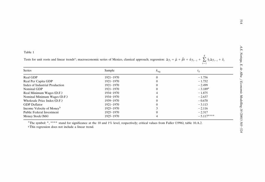
Ž .We start by applying augmented Dickey�Fuller ADF tests for a unit root in aŽ .model without a structural break, that is, we estimate Eq. 5 imposing the

restriction � � � � 0. The results are presented in Table 1. For most of the seriesthe unit root hypothesis can not be rejected. Exceptions are Nominal GDP, for

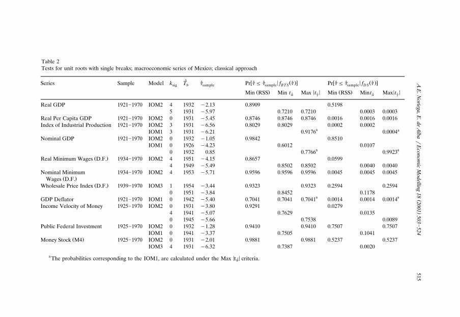
Ž .which the rejection is marginal 10% critical value � �3.18 , and the M4 series. Itseems to be that either there is a unit root in most of Mexican macroeconomictime series, or the particular shape of our DGP for modelling the long runbehavior of the data is mistaken; the economy did not evolve at a constant rateduring the sample period. This in turn biases the results towards non-rejection. So,in order to compete against the null, we need a better equipped alternative.Following the motivation discussed in Section 2, we extend our empirical analysisby allowing the presence of a structural break in the trend function. Table 2reports the results for the classical approach, of using models 1 and 2 under the

Ž .Innovational Outlier version labeled IOM1 and IOM2, respectively .As mentioned in Section 2, many of the series show an apparent break in their

trend function around the beginning of the 1930s; very close to the beginning ofthe sample. Setting k � 5 allows the procedures to detect this apparent break.max

Ž .Setting a higher value for k i.e. k � 10 induces the procedure not to detectmax maxit, but to detect ‘a second’ break in the sample, and reduces the already limitednumber of degrees of freedom. Column 4 shows the estimated lag length, k . Insigcolumn 6, represents the estimated t-statistic for testing the null hypothesissampleof a unit root, once allowance is made for an endogenously determined break datein the trend function, under three different criteria for the selection of the breakdate. The results are extracted from columns 7�9 and 10�12, which show theposition where this sample estimate of the t-statistic lies relative to the simulated

� �density functions under both the BTS and DS hypotheses, denoted Pr ˆ sampleŽ .� � � Ž .�f and Pr f , respectively. These are calculated for each oneˆ ˆ ˆ ˆBTS sample DS

Ž .of the minRSS, Min t , and Max t Max criteria.ˆ� �� ˆ ˆLet us interpret some of the results in Table 2. For Real per capita GDP, for

Ž .instance, all three criteria coincided in the selected break year 1931 , the IOŽ . Ž .model type IOM2 , and the lag length k � 0 . The probabilities shown insig

columns 7�9 and 10�12 indicate support for the BTS model, and a clear rejectionof the DS one, respectively, under all three criteria. The same analysis applies toGDP Deflator. For the Index of Industrial Production, the same conclusion can bereached regarding these probabilities. However, the selected model depends on thecriterion for determining the break date: both minRSS and Min t select the�

()

A.E

.Noriega,E

.deA

lba�

Econom

icM

odelling18

2001503

�524514

Table 1k

a ˆTests for unit roots and linear trends ; macroeconomic series of Mexico, classical approach; regression: y � � � � t � � y � � y � �ˆ ˆ ˆ ˆÝt t�1 i t� i ti�1

Series Sample k tsig �

Real GDP 1921�1970 0 �1.756Real Per Capita GDP 1921�1970 0 �1.732Index of Industrial Production 1921�1970 0 �2.499

�Nominal GDP 1921�1970 0 �3.189Ž .Real Minimum Wages D.F. 1934�1970 4 �1.875

Ž .Nominal Minimum Wages D.F. 1934�1970 4 �2.637Ž .Wholesale Price Index D.F. 1939�1970 0 �0.670

GDP Deflator 1921�1970 0 �3.113bIncome Velocity of Money 1925�1970 3 �2.116

Public Federal Investment 1925�1970 0 �2.317��Ž .Money Stock M4 1925�1970 4 �5.117

a � �� Ž .The symbol: , stand for significance at the 10 and 1% level, respectively; critical values from Fuller 1996 , table 10.A.2.b This regression does not include a linear trend.

()

A.E

.Noriega,E

.deA

lba�

Econom

icM

odelling18

2001503

�524515

Table 2Tests for unit roots with single breaks; macroeconomic series of Mexico; classical approach

ˆ � � Ž .� � � Ž .�Series Sample Model k T Pr f Pr f ˆ ˆ ˆ ˆ ˆ ˆ ˆsig b sample sample BT S sample D S

Ž . � � Ž . � �Min RSS Min t Max t Min RSS Min t Max t� � � �ˆ ˆ ˆ ˆ

Real GDP 1921�1970 IOM2 4 1932 �2.13 0.8909 0.51985 1931 �5.97 0.7210 0.7210 0.0003 0.0003

Real Per Capita GDP 1921�1970 IOM2 0 1931 �5.45 0.8746 0.8746 0.8746 0.0016 0.0016 0.0016Index of Industrial Production 1921�1970 IOM2 3 1931 �6.56 0.8029 0.8029 0.0002 0.0002

a aIOM1 3 1931 �6.21 0.9176 0.0004Nominal GDP 1921�1970 IOM2 0 1932 �1.05 0.9842 0.8510

IOM1 0 1926 �4.23 0.6012 0.0107a a0 1932 0.85 0.7766 0.9923

Ž .Real Minimum Wages D.F. 1934�1970 IOM2 4 1951 �4.15 0.8657 0.05994 1949 �5.49 0.8502 0.8502 0.0040 0.0040

Nominal Minimum 1934�1970 IOM2 4 1953 �5.71 0.9596 0.9596 0.9596 0.0045 0.0045 0.0045Ž .Wages D.F.

Ž .Wholesale Price Index D.F. 1939�1970 IOM3 1 1954 �3.44 0.9323 0.9323 0.2594 0.25940 1951 �3.84 0.8452 0.1178

a aGDP Deflator 1921�1970 IOM1 0 1942 �5.40 0.7041 0.7041 0.7041 0.0014 0.0014 0.0014Income Velocity of Money 1925�1970 IOM2 0 1931 �3.80 0.9291 0.0279

4 1941 �5.07 0.7629 0.01350 1945 �5.66 0.7538 0.0089

Public Federal Investment 1925�1970 IOM2 0 1932 �1.28 0.9410 0.9410 0.7507 0.7507IOM1 0 1941 �3.37 0.7505 0.1041

Ž .Money Stock M4 1925�1970 IOM2 0 1931 �2.01 0.9881 0.9881 0.5237 0.5237IOM3 4 1931 �6.32 0.7387 0.0020

a � �The probabilities corresponding to the IOM1, are calculated under the Max t criteria.�


IOM2, while Max t selects the IOM1. Hence, under either model, there does notˆ��

seem to be support for the DS null. For Income Velocity of Money, all three criteriacoincided in the IO model type. However, there is no coincidence in the estimationof the break year. There seem to be two breaks in this series, the first in 1931 andthe second one around the early 1940s. Taking into account any of these two, theDS specification can be rejected. For Nominal Minimum Wage, all three criteriacoincide in rejecting the DS null. However, the BTS alternative does not seem tobe supported either. For Wholesale Price Index, although neither specification canbe rejected, the DS one seems more plausible than the TS one.

For the rest of the series, the results depend on the criterion used for selectingthe break date. For instance, for Real GDP, the DS model can be strongly rejectedwhile the TS one can not under both the Min t and the Max t criteria.� �� ˆ ˆHowever, under the min RSS the results indicate that neither specification can berejected. For Nominal GDP the p-values make clear that the value of undersamplethe min RSS criterion could hardly have been generated from the BTS specifica-tion. On the other hand, there is no strong evidence against the DS one. Thisresult is reversed for the Min t criterion, under which the selected model and�

break date are different. The Max t selects yet a different break year and yieldsˆ��

Ž .an explosive root. As can be deduced from Perron’s 1997, p.356 arguments, theŽ .use of the Min t and the Max t or Max t criteria imply a systematic attemptˆ� �� ˆ ˆ

to maximize the chances of rejecting a unit root, or to maximize the chances offinding the most likely date of a break, respectively. In trying not to bias our resultsin any of these directions we rely on the minRSS criterion, which ensures the bestfitting model, for those series for which conflicting results were obtained. Hence,for Nominal GDP, Public Federal In�estment, and Money Stock, the probabilitiesfavour more the DS than the BTS specification. The inverse is true for RealMinimum Wages. Finally, for Real GDP, the DS model is much more plausiblethan the BTS one.

In summary, for six series the DS specification can be rejected. For other three,Nominal GDP, Public Federal In�estment, and Money Stock, the unit root hypothe-sis cannot be rejected. Finally, for Real GDP and the Wholesale Price Index, neitherthe DS nor the BTS models can be rejected. For all of the production variablesthe structural break was estimated around 1930, as expected from the discussion inSection 2. Real and Nominal Wages show a break in the early 1950s. In contrastwith the no break results presented above, it seems that there is not a unit root inmany of the analyzed macroeconomic time series.9 The break around 1930 had thepower to alter the long run trend of many variables. Ignoring this break would haveimplied accepting the presence of a unit root in most of the variables.10

9As a simple robustness analysis, we applied standard ADF tests to data from T � 1 to 1970. Thebresults from this analysis confirm our unit root evidence allowing for a break.

10 Ž .This is evident in the classical approach. In the Bayesian approach, the values for Pr � 0.975 � DTdid decrease for almost all series under all the priors. However, there were some cases where in factthey increased.


4.2. Bayesian analysis

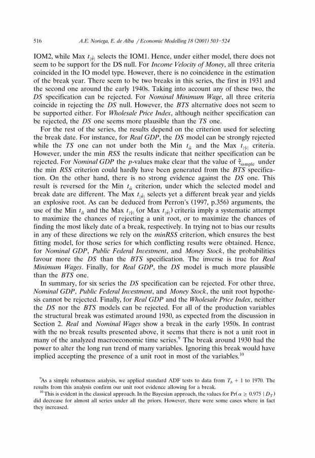
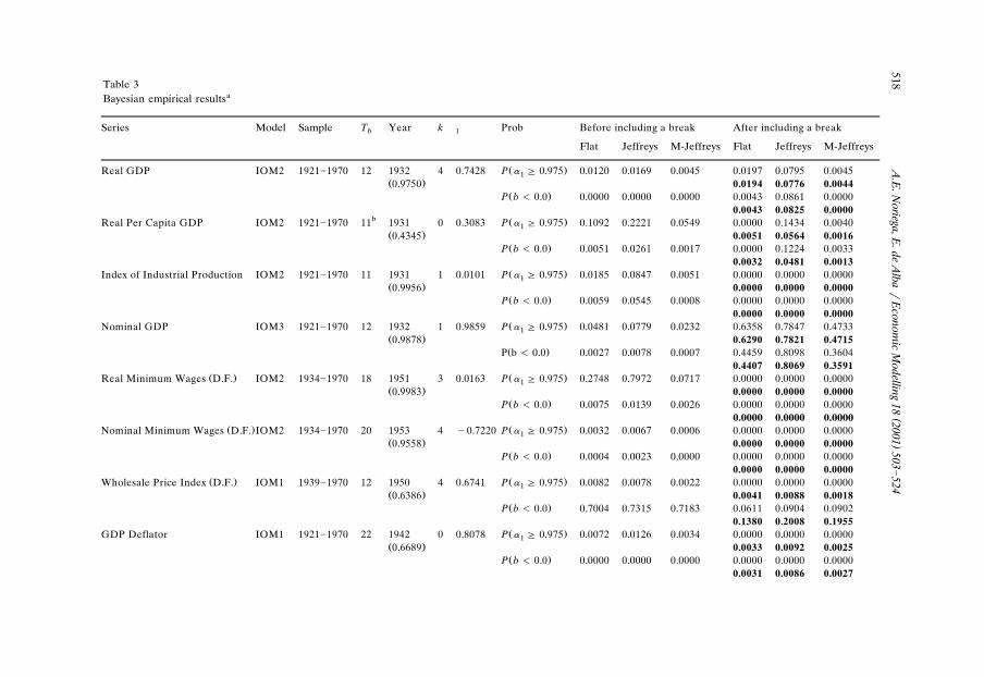
Table 3 summarizes the results of applying the Bayesian methods mentioned inSection 3.2 to the Mexican macroeconomic series. We will carry out our analyses

Ž . Ž .along the lines of Phillips 1991 , and Zivot and Phillips 1994 . It is based onŽ . Ž .Pr � 0.975 � D and Pr b 0.0 � D . The former is the probability of ‘near1 T T

Ž .non-stationarity’ of Phillips 1991 . Values of this probability larger than 5%Ž .indicate the presence of a unit root. Similarly, Pr b 0.0 � D � 0.05 indicatesT

absence of a linear trend. In the applications the ‘change in trend’ parameter, � , isused to model the behavior of the series prior to the break. This way, in most ofthe series the value of b is expected to be positive, since they initially decrease andhave a positive trend after the break. This means that the definition of thedummies is slightly different than stated in the theoretical model, but the conclu-

Ž .sions do not change. Zivot and Phillips 1994 are implicitly assuming that allŽ � .trends are positive, before and after the breaks. The analysis of Pr b 0.01 DT

in their paper only makes sense under this assumption.For each macroeconomic series, the first columns of Table 3 gives the type of

model selected, the years of data included in the sample, the moment the breaktakes place, T , the corresponding year of the break, the selected value of kbŽ .number of lags minus one and the ‘estimate’ of � obtained when a break is1

Ž � .included in the model. Recall that T is the value such that p T y,�b b 0� Ž � .4� max p r y,� . The number in parentheses under the year is the actual value0

rŽ . Žof p T � y,� . The next three columns of this Table show the values of Pr � b 0 1

. Ž .0.975 � D and Pr b 0.0 � D computed before including a trend break in theT Tmodel. The numbers in the last three columns of the Table are the values ofŽ . Ž .Pr � 0.975 � DT ,r � T and Pr b 0.0 � D ,r � T , i.e. the conditional1 b T b

probabilities given the break at T . The bold numbers in these last columnsbŽ . Ž .correspond to the values of Pr � 0.975 � D and Pr b 0.0 � D computed1 T T

Ž . Ž .using the marginal unconditional density 16 as follows

�Ž � . �Pr � 0.975 D � p � y ,� d�Ž .H1 T i 1 0 1

0.975

�T�2 � �� Ý p r y , � p � y ,� ,r d�Ž . Ž .H r�2 i 0 i i 0 1

0.975

Ž .for i � F, J, MJ. With an analogous expression for Pr b 0.0 � D . In both cases,Tbefore and after including a break, results are obtained from the posteriordistributions using ‘flat’, Jeffreys and Modified�Jeffreys priors. Jeffreys’ modifiedprior was obtained with � � 0.03 in all cases. This is within the range suggested by

Ž .Zivot and Phillips 1994 . Sensitivity tests showed that in general there were nosubstantial differences when other values were used.

The value of k obtained by applying the Schwarz criterion varies from series toseries taking values between zero and four. Thus, the bias towards small values that

Ž .Ng and Perron 1995 found in the information-based criteria for determining k

()

A.E

.Noriega,E

.deA

lba�

Econom

icM

odelling18

2001503

�524518Table 3

aBayesian empirical results

Series Model Sample T Year k Prob Before including a break After including a breakb 1

Flat Jeffreys M-Jeffreys Flat Jeffreys M-Jeffreys

Ž .Real GDP IOM2 1921�1970 12 1932 4 0.7428 P � 0.975 0.0120 0.0169 0.0045 0.0197 0.0795 0.00451Ž .0.9750 0.0194 0.0776 0.0044

Ž .P b � 0.0 0.0000 0.0000 0.0000 0.0043 0.0861 0.00000.0043 0.0825 0.0000

b Ž .Real Per Capita GDP IOM2 1921�1970 11 1931 0 0.3083 P � 0.975 0.1092 0.2221 0.0549 0.0000 0.1434 0.00401Ž .0.4345 0.0051 0.0564 0.0016

Ž .P b � 0.0 0.0051 0.0261 0.0017 0.0000 0.1224 0.00330.0032 0.0481 0.0013

Ž .Index of Industrial Production IOM2 1921�1970 11 1931 1 0.0101 P � 0.975 0.0185 0.0847 0.0051 0.0000 0.0000 0.00001Ž .0.9956 0.0000 0.0000 0.0000

Ž .P b � 0.0 0.0059 0.0545 0.0008 0.0000 0.0000 0.00000.0000 0.0000 0.0000

Ž .Nominal GDP IOM3 1921�1970 12 1932 1 0.9859 P � 0.975 0.0481 0.0779 0.0232 0.6358 0.7847 0.47331Ž .0.9878 0.6290 0.7821 0.4715

Ž .P b � 0.0 0.0027 0.0078 0.0007 0.4459 0.8098 0.36040.4407 0.8069 0.3591

Ž . Ž .Real Minimum Wages D.F. IOM2 1934�1970 18 1951 3 0.0163 P � 0.975 0.2748 0.7972 0.0717 0.0000 0.0000 0.00001Ž .0.9983 0.0000 0.0000 0.0000

Ž .P b � 0.0 0.0075 0.0139 0.0026 0.0000 0.0000 0.00000.0000 0.0000 0.0000

Ž . Ž .Nominal Minimum Wages D.F. IOM2 1934�1970 20 1953 4 �0.7220 P � 0.975 0.0032 0.0067 0.0006 0.0000 0.0000 0.00001Ž .0.9558 0.0000 0.0000 0.0000

Ž .P b � 0.0 0.0004 0.0023 0.0000 0.0000 0.0000 0.00000.0000 0.0000 0.0000

Ž . Ž .Wholesale Price Index D.F. IOM1 1939�1970 12 1950 4 0.6741 P � 0.975 0.0082 0.0078 0.0022 0.0000 0.0000 0.00001Ž .0.6386 0.0041 0.0088 0.0018

Ž .P b � 0.0 0.7004 0.7315 0.7183 0.0611 0.0904 0.09020.1380 0.2008 0.1955

Ž .GDP Deflator IOM1 1921�1970 22 1942 0 0.8078 P � 0.975 0.0072 0.0126 0.0034 0.0000 0.0000 0.00001Ž .0.6689 0.0033 0.0092 0.0025

Ž .P b � 0.0 0.0000 0.0000 0.0000 0.0000 0.0000 0.00000.0031 0.0086 0.0027

()

A.E

.Noriega,E

.deA

lba�

Econom

icM

odelling18

2001503

�524519

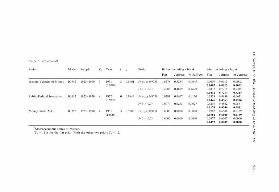
Ž .Table 3 Continued

Series Model Sample T Year k Prob Before including a break After including a breakb 1

Flat Jeffreys M-Jeffreys Flat Jeffreys M-Jeffreys

Ž .Income Velocity of Money IOM2 1925�1970 7 1931 3 0.5401 P � 0.975 0.0278 0.5234 0.0045 0.0007 0.0013 0.00021Ž .0.9999 0.0007 0.0013 0.0002

Ž .P b � 0.0 0.4886 0.4679 0.4679 0.0412 0.7215 0.72150.0412 0.7214 0.7214

Ž .Public Federal Investment IOM2 1925�1970 8 1932 0 0.8944 P � 0.975 0.0291 0.0667 0.0120 0.1539 0.4889 0.06311Ž .0.9122 0.1446 0.4563 0.0596

Ž .P b � 0.0 0.0070 0.0263 0.0027 0.1239 0.4562 0.05610.1174 0.4346 0.0541

Ž . Ž .Money Stock M4 IOM2 1925�1970 7 1931 3 0.7806 P � 0.975 0.0000 0.0000 0.0000 0.0762 0.6506 0.01591Ž .1.0000 0.0762 0.6506 0.0159

Ž .P b � 0.0 0.0000 0.0000 0.0000 0.0477 0.0007 0.00000.0477 0.0007 0.0000

aMacroeconomic series of Mexico.bT � 11 is for the flat prior. With the other two priors T � 12.b b


does not seem to be evident. In addition, a look at the Ljung�Box Q-statistic ineach case did not indicate existence of autocorrelation in the residuals. A commentis in order regarding k. The value k � 3 used for the Income Velocity of Money and

Ž .the Money Stock M4 is not the one obtained by the application of Schwarz, whichin both cases resulted in k � 5. However, due to the fact that the apparent breakpoint of each series is located at observation 7, then using k � 1 � 6 lags in themodel would actually leave the change point at the second observation. It is notpossible to fit the model in this case, due to numerical instabilities. Nevertheless,

Ž .all are well within the range of values in Nelson and Plosser 1982 , or Zivot andŽ .Phillips 1994 .

In general, a fairly large probability of a break results for one point of eachseries, with some having two or three smaller ones. In most of the series the breakis detected at or near 1932. The exceptions are the three series related to Mexico

Ž .City D.F. , with a break around 1951, and GDP Deflator which shows a break at1942. Except for Real Per Capita GDP, the probability of a break is greater than0.5. This series shows a relatively low value for this probability: 0.4345. It could beinterpreted in the sense that there are actually no breaks in the trend. For the

Ž . Žposterior pmd p r � y,� for Real Per Capita GDP, we have that p T � 11 ori 0 b.T � 12 � y,� � 0.4345 � 0.3440 � 0.7785. It is evident that there is a highb 0

probability of a break point, but it is not clear if it is located at T � 11 or atbT � 12.b

The results show that Jeffreys’ prior generally yields a posterior distribution withŽ .a higher value for Pr � 0.975 � D . In fact, there is a substantial posterior1 T

probability of explosive values for � . Jeffreys’ modified prior corrects this effect1and tends to show values of this probability that can be even lower than for the flatprior.

Ž . Ž .Zivot and Phillips 1994 use Pr � 0.975 � D to evaluate the presence of a1 TŽ .unit root, together with Pr b 0.0 � D . If both of these probabilities are ‘large’ itT

is taken as an indication of the presence of a unit root. It is not clear why a largevalue of this last probability is an indication of the presence of unit roots. Theirimplied argument would be that if � is near 1 and b is not positive then it must1be 0. Analysis of these probabilities, before including a break in the trend,indicates evidence of a unit root only in Real Per Capita GDP and Real Minimum

Ž .Wages D.F. . On the other hand the Wholesale Price Index and the Income VelocityŽ .of Money show very large values for Pr b 0.0 � D . In the case of the WholesaleTŽ .Price Index this indicates that once the five lags are incorporated in the model

there is no need for a trend parameter. For the Income Velocity of Money it simplyconfirms the absence of a clear trend evident in the plot of the series. The value ofŽ .Pr � 0.975 � D , before allowance is made for a break in trend, is large only1 T

Ž .for Real Per Capita GDP and Real Minimum Wages D.F. . This holds for allpriors. Thus, there is evidence in favor of the presence of a unit root only for thesetwo series, when no allowance is made for a break in the trend. This is in general

Ž .agreement with the kind of results obtained by Zivot and Phillips 1994 who findthat the unit root hypothesis is not implausible only in five of the 14 series in

Ž .Nelson and Plosser 1982 .


Some authors indicate that the use of a flat prior biases the analysis against theŽ .unit root hypothesis Phillips, 1991 . Looking at the results in the two columns in

Table 3 corresponding to the flat prior, it is apparent that in three cases theprobability increases after the break is introduced: Nominal GDP, Public FederalIn�estment and Money Stock. This might be a reflection of the fact that theintroduction of the break in trend corrects the bias. However, this occurs with allpriors. In fact if one looks at the probability in all three models before allowing forthe break in trend it would seem that the modified Jeffreys prior is also biasedagainst the unit root hypothesis and perhaps even more so than the flat prior.Modifying � � 0.03 to � � 0.05 does not alter the conclusions.

Allowing for a break in the time series at T , if one looks at the conditionalbŽ .posterior probability Pr � 0.975 � D , r � T derived using the flat prior, the1 T b

Ž .largest values occur for Nominal GDP 0.6358 and Public Federal In�estmentŽ . Ž . Ž .0.1539 . A similar conclusion holds for Money Stock M4 0.0762 but not asstrongly. The previous results are not as clear under the Modified Jeffreys prior.The probability is still larger than 0.05 only in the first two series. Hence, from aBayesian point of view, there is evidence of a unit root only in these three of the 11Mexican macroeconomic series. Surprisingly, this is supported both by the modifiedJeffreys and flat priors. The results hold with the conditional as well as with themarginal probabilities.

5. Discussion and conclusions

The application of classical and Bayesian methods for testing for a unit rootunder endogenous structural breaks, allows us to arrive at some common conclu-sions. This should come as no surprise especially if one considers that the min RSScriterion used in the classical analysis is nearly inversely proportional to the

Ž . Ž .Bayesian criterion used here. To see this consider that in Eqs. 13 � 15 we canwrite:

Ž .� T�k�4 �2� Ž Ž ..p r y ,� � h X , y ,r m u r i � F , J ,MJˆŽ .Ž .i 0

Ž Ž .. Ž . Ž .but m u r � min RSS and so approximately p r � y,� � h X , y,r �ˆ r i 0Ž .�ŽT�k�4.�2minRSS . The fact that the result is not exact explains why we do notrget the same results every time.

The first conclusion is that the estimated break dates are nearly identical acrossapproaches, specially under the min RSS criterion under the classical approach. Inparticular, both approaches detect the presence of a structural break during theearly 1930s for the production variables, Income Velocity of Money, Public FederalIn�estment, and M4; during the early 1950s for Real and Nominal Wages and thePrice Index, and during the early 1940s for the GDP Deflator. The first findingrelates to the conditions created during the period 1921�1933: the creation of the

Ž .central bank 1925 , the shift of public spending from administrative spending to


‘promotion of economic growth’ spending, the departure from the gold standardŽ .1931 , and the important devaluation in 1933. These conditions allowed theeconomy to set on a new long-run trend, with much higher growth rates. Forinstance, for Real GDP and Real Per Capita GDP the growth rates for the1921�1931 period are 0.41 and �1.19%, respectively. For the 1932�1970 periodthese rates are 5.71 and 2.96%.

Second, the results on the rejection of the unit root hypothesis are much moresensitive to the trend function’s specification under the classical approach thanunder the Bayesian approach. Before a break in the trend is allowed, the classicalresults do not reject the null hypothesis for most series, while the Bayesian

Ž .framework leads to favor trend stationarity when using a flat or an M-Jeffreysprior, except for Real GDP and Real Minimum Wages. Perhaps this is due to the

Ž .tendency to favor trend stationarity noted by Phillips 1991 . This suggests that thebias towards non-rejection which results from ignoring the presence of a break

Ž .found in Perron 1989 and others does not really exist under the Bayesianapproach. Even though the breaks found are quite significant for most series � asthe probabilities in Table 3 reveal � their inclusion in the model does not seem tobe decisive in rejecting the unit root hypothesis. However, once allowance is madefor the break points, the results of both approaches are in more general agreement.This may be an indication that once a high probability of a break point has beendetected, then any further analysis should be done taking this into account.

Under the classical approach, the unit root hypothesis does not seem to besupported by our historical data set for the Mexican economy, once allowance ismade for the estimation of a single break. Exceptions of this are Nominal GDP,Public Federal In�estment, M4, and Wholesale Price Index. Note that for the firstthree of these, the probability of near non-stationarity increases after including abreak in the trend function under the Bayesian approach. In fact, the unit root can

Ž .be rejected for these three series only under a linear no break trend function. Wesuspect that this phenomenon may be the result of the presence of multiple breaksin the trend function of these series. This holds under either the classical or theBayesian approaches: allowing for multiple breaks in the trend drastically reduces

Ž .the posterior probability of a unit root Pr � 0.975 � D ,r � T ,r � T ,.. and1 T 1 b1 2 b2the classical test rejects the null hypothesis of a unit root. Both Bayesian andclassical analyses show ample evidence of at least one more break in Nominal GDPand Public Federal In�estment. The details of these analyses will be publishedelsewhere.

The results for Nominal GDP, Public Federal In�estment and M4 suggests thatnon-rejection of the unit root hypothesis means that it was not possible to identifya trend around which the cycle is stationary. In other words, the estimated trend isnot the long-run movement of the economy around which the business cyclefluctuates in a stationary fashion. The reason is that the models themselves restrictthe class of secular movements we can estimate from the data. Some knowledge or‘structure’ about the long-run movements of the economy is needed before we tryto analyze the short-run fluctuations as a ‘residual’ component.


Acknowledgements

With thanks to Araceli Ramırez for excellent research assistance and helpful´Žcomments. Financial support for Consejo Nacional de Ciencia y Tecnologıa CON-´

.ACYT , Mexico, is gratefully acknowledged.

References

Ž .Bai, J., 1997a. Estimating multiple breaks one at a time. Econom. Theory 13 3 , 315�352.Ž .Bai, J., 1997b. Estimation of a change point in multiple regression models. Rev. Econ. Stat. 79 4 ,

551�563.Bai, J., Perron, P., 1998a. Estimating and testing linear models with multiple structural changes.

Ž .Econometrica 66 1 , 47�78.Bai, J., Perron, P., 1998b. Computation and Analysis of Multiple Structural Change Models. mimeo.

Ž .de Jong, D.N., 1996. A Bayesian search for structural breaks in US GNP. In: Fomby, T.B. Ed. , in:Advances in Econometrics Part B, 11. JAI Press, pp. 109�146.

Diebold, F.X., Senhadji, A.S., 1996. The uncertain unit root in Real GNP: Comment. Am. Econ. Rev. 86Ž .5 , 1291�1298.

Fuller, W., 1996. Introduction to Statistical Time series, 2nd Wiley.Lubrano, M., 1995. Testing for unit roots in a Bayesian framework. J. Econom. 69, 81�109.Maddala, G.S., Kim, I.M., 1996. Structural change and unit roots. J. Stat. Plann. Inference 49, 73�103.Nelson, C.R., Plosser, C., 1982. Trends and random walks in macroeconomic time series: some evidence

and implications. J. Monet. Econ. 10, 139�162.Ng, S., Perron, P., 1995. Unit root tests in ARMA models with data dependent methods for the selection

of the truncation lag. J. Am. Stat. Assoc. 90, 268�269.Ouliaris S., Phillips P.C.B., 1995. COINT 2.0. GAUSS. Procedures for Cointegrated Regressions.

Aptech Systems, Inc.Perron, P., 1989. The great crash, the oil price shock, and the unit root hypothesis. Econometrica 57,

1361�1401.Perron, P., 1992. Trend, unit root and structural change: a multi-country study with historical data. in

Proceedings of the Business and Economic Statistics Section. American Statistical Association, pp.144�149.

Perron, P., 1993. Trend, unit root and structural change in macroeconomic time series. Department ofŽ .Economics, Universite de Montreal, Mimeo. In: Rao, B.B. Ed. , In Cointegration for the Applied´ ´

Economist. MacMillan Press.Perron, P., 1997. Further evidence on breaking trend functions in macroeconomic variables. J. Econom.

80, 355�385.Phillips, P.C.B., 1991. To criticize the critics: an objective Bayesian analysis of stochastic trends. J. Appl.

Econom. 6, 333�364.Poirier, D.J., 1995. Intermediate Statistics and Econometrics. MIT Press, Cambridge.Rudebusch, G.D., 1992. Trends and random walks in macroeconomic time series: a re-examination. Int.

Ž .Econ. Rev. 33 3 , 661�680.Ž .Rudebusch, G.D., 1993. The uncertain unit root in real GNP. Am. Econ. Rev. 83 1 , 264�272.

Said, E.S., Dickey, D.A., 1984. Testing for unit roots in autoregressive-moving average models ofunknown order. Biometrika 71, 599�607.

Sims, C.A., 1988. Bayesian skepticism on unit root econometrics. J. Econ. Dyn. Control 12, 463�474.Ž .Solıs, L., 1970. La Realidad Economica Mexicana: Retrovision y Perspectivas. In: Siglo XXI Ed. . 1st´ ´ ´

edition.


Stock, J.H., 1994. Unit roots, structural breaks and trends. Chapter 46. In: Engle, R., McFadden D.,Ž .Eds. . Handbook of Econometrics. North Holland.

Tsurumi, H., Wago, H., 1996. A Bayesian analysis of unit root and cointegration with an application to aŽ .yen�dollar exchange rate model. In: Fomby, T.B. Ed. , in: Advances in Econometrics Part B, 11.

JAI Press, pp. 51�88.Zivot, E., Phillips, P.C.B., 1994. A Bayesian analysis of trend determination in economic time series.

Ž .Econom. Rev. 13 3 , 291�336.

Stationarity and structural breaks — evidence from classical and Bayesian approaches

Documents

Transcript of Stationarity and structural breaks — evidence from classical and Bayesian approaches