2011/55

■

Estimating and forecasting structural breaks in financial time series

Luc Bauwens, Arnaud Dufays and Bruno de Backer

Center for Operations Research and Econometrics

Voie du Roman Pays, 34

B-1348 Louvain-la-Neuve Belgium

http://www.uclouvain.be/core

D I S C U S S I O N P A P E R

CORE DISCUSSION PAPER 2011/55

Estimating and forecasting structural breaks in financial time series

Luc BAUWENS 1, Arnaud DUFAYS2

and Bruno DE BACKER 3

November 2011

Abstract We present an algorithm, based on a differential evolution MCMC method, for Bayesian inference in AR-GARCH models subject to an unknown number of structural breaks at unknown dates. Break dates are directly treated as parameters and the number of breaks is determined by the marginal likelihood criterion. We prove the convergence of the algorithm and we show how to compute marginal likelihoods. We allow for both pure change-point and recurrent regime specifications and we show how to forecast structural breaks. We illustrate the efficiency of the algorithm through simulations and we apply it to eight financial time series of daily returns over the period 1987-2011. We find at least three breaks in all series.

Keywords: Bayesian inference, structural breaks, differential evolution, change-point, recurrent states, break forecasting, marginal likelihood.

JEL Classification: C11, C15, C22, C58

1 Université catholique de Louvain, CORE, B-1348 Louvain-la-Neuve, Belgium. E-mail: luc.bauwens@uclouvain.be. This author is also member of ECORE, the association between CORE and ECARES. 2 Université catholique de Louvain, CORE, B-1348 Louvain-la-Neuve, Belgium. E-mail: arnaud.dufays@uclouvain.be. 3 Bruno de Backer started working on this project during his studies at the LSE.

We thank Christian Julliard for his helpful comments and suggestions. We are also grateful to participants to the workshop on Econometric and Statistical Modelling of Multivariate Time Series 2011 at Université catholique de Louvain and the 10th OxMetrics Users’ Conference at Maastricht University. Research supported by the contract ”Projet d’Actions de Recherche Concertées” 07/12-002 of the ”Communauté française de Belgique”, granted by the ”Académie universitaire Louvain”.

This paper presents research results of the Belgian Program on Interuniversity Poles of Attraction initiated by the Belgian State, Prime Minister's Office, Science Policy Programming. The scientific responsibility is assumed by the authors.

1 Introduction

The class of Generalized AutoRegressive Conditional Heteroskedastic (GARCH) models (see

Engle (1982), and Bollerslev (1986)) has been widely applied to different kinds of time series

since it is a simple and powerful way to model volatility. Nowadays, GARCH volatility models

with fixed parameters are known to be too restrictive for long time series due to breaks in

the volatility process.

Ignoring structural breaks generally produces poor forecasts and often gives the spurious

impression of a nearly integrated behaviour of the time series (see, e.g., Diebold (1986),

Lamoureux and Lastrapes (1990), and Hillebrand (2005)). Moreover, GARCH processes

imply that long-run forecasts of conditional volatility tend to the unconditional variance of

the error term in the mean equation. In order to tackle these issues more flexible models have

been designed. They can be split into three categories: Component and smooth transition

models (e.g. Amado and Terasvirta (2008)), Markov-switching models (e.g. Gray (1996),

Haas, Mittnik, and Paolella (2004), Bauwens, Preminger, and Rombouts (2010), and He and

Maheu (2010)), and models with time-varying unconditional variance (e.g. Engle and Rangel

(2008)). In this paper we focus on change-point and recurrent state models. These models

assume that structural changes can happen in an economy and affect the parameters of the

considered econometric model but do not change the nature of the model itself.

Dealing with structural breaks is usually done by applying the forward-backward algo-

rithm introduced by Chib (1996). However, the method cannot be applied to models with

path dependence (see Fruhwirth-Schnatter (2004)) since the number of computations to be

performed by the computer grows exponentially with the length of the time series. Indeed,

path dependence is the fact that any value of the series depends on all the previous ones. For

instance, ARMA and GARCH processes can be path dependent in the mean (cfr. ARMA)

and conditional variance (cfr. GARCH).

Four recent papers tackle the issue of path dependence, all of them focusing on GARCH

models. He and Maheu (2010) use a Sequential Monte Carlo on-line method in order to

tell whether a break occurs when a new observation becomes available. Hence, their method

is more useful to forecasting rather than detecting purposes. On the contrary, Liao (2008),

Bauwens, Preminger, and Rombouts (2010), and Bauwens, Dufays, and Rombouts (2011)

develop off-line MCMC methods. Similarly to the present work, Liao (2008) considers the

1

break dates as parameters to be estimated and not anymore as hidden states underlying the

data generating process. Liao (2008) separates the problem into two parts: drawing the model

parameters and drawing the break dates. She uses a standard Gibbs sampler for the model

parameters and chooses to draw the break dates via the Griddy-Gibbs method (see Bauwens,

Lubrano, and Richard (1999)). She also proposes a sequential technique to determine the

number of breaks in a series which is very different from what is done in this work. Still

considering MCMC methods, the approach in Bauwens, Preminger, and Rombouts (2010)

does not mix well because the sampling of the variables suffers from huge correlations across

iterations of the algorithm. This problem is circumvented in Bauwens, Dufays, and Rombouts

(2011) by embedding a Sequential Monte Carlo technique inside an MCMC algorithm. This

approach works well and allows to compute marginal likelihoods for model selection but is

computationally demanding.

The technical articles that influence the present paper are ter Braak and Vrugt (2008) and

Vrugt, ter Braak, Diks, Robinson, Hyman, and Higdon (2009). ter Braak and Vrugt (2008)

propose a Differential Evolution Markov Chain (DEMC) algorithm in which the proposal of

the Metropolis algorithm is automatically generated. An extension of this algorithm is the

DiffeRential Adaptative Evolution Metropolis (DREAM) algorithm of Vrugt, ter Braak, Diks,

Robinson, Hyman, and Higdon (2009). In this paper we derive a Discrete-DREAM algorithm

in order to sample the break dates in a Metropolis-type of block-at-a-time algorithm. We

prove the convergence of our MCMC algorithm to the stationary distribution.

We thus introduce a novel MCMC method which deals with change-points in time series

models and computes the resulting marginal likelihood. The proposed algorithm has the

advantage to accommodate path dependence problems and to be fast to converge and easy to

implement. Our specification allows for recurrent states which is a class of structural break

model somewhere between Change-Point and Markov-Switching models. Moreover we also

introduce a hierarchical structure to forecast structural break in the spirit of what Pesaran,

Pettenuzzo, and Timmermann (2006) did for autoregressive models.

The paper is organized as follows. In section 2, we present the DREAM algorithm that we

adapt to the present context of structural breaks. In section 3, we explain how to deal with the

unknown number of breaks using the marginal likelihood criterion. In section 4, we propose

two improvements, namely how to allow for recurrent regimes and how to forecast future

2

breaks. In section 5, we test the efficiency of the new algorithm by means of simulations.

In section 6, we apply the algorithm on daily data for the S&P500 index and give summary

statistics for seven other financial series. Section 7 concludes.

2 D-DREAM Algorithm

For the sake of simplicity, the present discussion focuses on an AR(1)-GARCH(1,1) spec-

ification though the algorithm could easily be adapted to more general models such as

ARMA(p,q)-GARCH(r,s) and many other time series models.

We denote by YT = (y1, ..., yT )′ a time series of T observations. Instead of considering a

whole vector of states as in Chib (1996), we focus on the break dates Γ = (τ1, ..., τK)′, with

the number of break dates K considered known for the moment. A Change-Point-AR(1)-

GARCH(1,1) model is thus characterized by the following set of equations:

yt = µk + φkyt−1 + εt,

εt = σtηt, with ηt ∼ i.i.d.N(0, 1),

σ2t = ck + αkε

2t−1 + βkσ

2t−1,

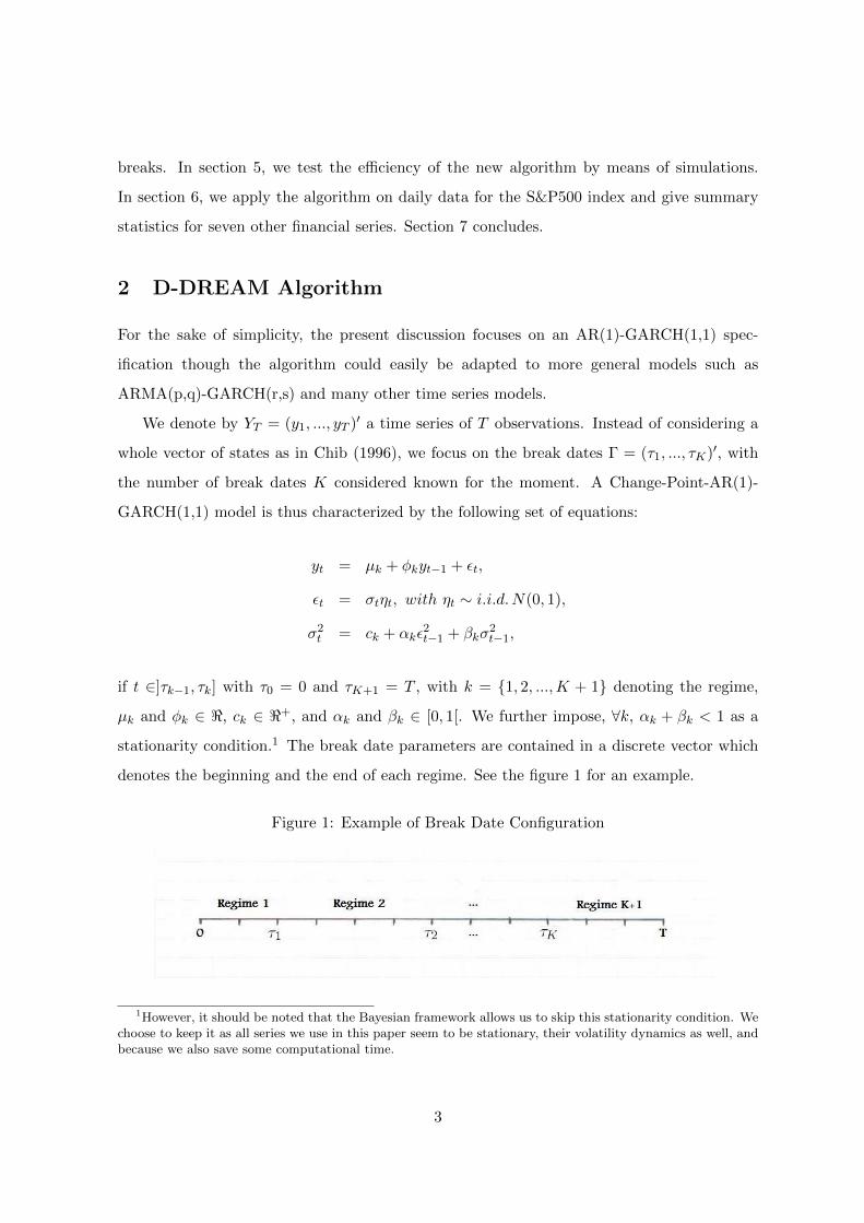
if t ∈]τk−1, τk] with τ0 = 0 and τK+1 = T , with k = {1, 2, ...,K + 1} denoting the regime,

µk and φk ∈ <, ck ∈ <+, and αk and βk ∈ [0, 1[. We further impose, ∀k, αk + βk < 1 as a

stationarity condition.1 The break date parameters are contained in a discrete vector which

denotes the beginning and the end of each regime. See the figure 1 for an example.

Figure 1: Example of Break Date Configuration

1However, it should be noted that the Bayesian framework allows us to skip this stationarity condition. Wechoose to keep it as all series we use in this paper seem to be stationary, their volatility dynamics as well, andbecause we also save some computational time.

3

Let Θ = (θ1, θ2, ..., θK+1)′ and θi = (µi, φi, ci, αi, βi), i.e. the parameters of the regime i. Our

MCMC scheme simply consists in drawing first from the posterior of the model parameters

Θ and, then, from the posterior of the break dates Γ as follows,

1. f(Θ|YT ,Γ)

2. f(Γ|YT ,Θ)

The difficulty is to sample from these two conditional densities since they have no closed form.

We detail now our Metropolis-type of procedure.

2.1 Sampling Θ

The full conditional distribution of Θ does not have any closed form but is proportional to

the likelihood times the prior:

f(Θ|YT ,Γ) ∝ f(YT |Θ,Γ)f(Θ)

Sampling from this distribution can be done by the Metropolis-Hastings (M-H) algorithm.

However the M-H algorithm is extremely versatile and depends on the proposal distribution.

ter Braak and Vrugt (2008) propose a Differential Evolution Markov Chain (DEMC) algorithm

in which the proposal of the Metropolis algorithm is automatically generated, that is, the size

and the direction of the jump are endogenously determined by the Markov Chains. The idea

is still to make a proposal from the previous draw to which a random term is added, however,

since they run multiple chains in parallel they can make these chains interact between each

other. An extension of this algorithm is the DiffeRential Adaptative Evolution Metropolis

(DREAM) algorithm of Vrugt, ter Braak, Diks, Robinson, Hyman, and Higdon (2009). They

show that the DREAM algorithm is more efficient than the DEMC algorithm in the sense

that it mixes better and thus converges faster. We use the DREAM algorithm to sample from

the full conditional distribution of Θ.

Following the DREAM algorithm, N Markov chains are launched and interact between

each other. The proposal of a new location for a given chain is indeed constructed from the

current locations of other chains. Focusing on the ith chain (i = 1, ..., N) at the t+1th MCMC

iteration, the procedure can be described in 3 steps.

4

1. Propose a new Θt+1i , denoted by Zi hereafter, according to the following rule (omitting

superscripts referring to iterations for simplicity):

Zi = Θi + γ(δ, d′)(

δ∑g=1

Θr1(g) −δ∑

h=1

Θr2(h)) + ε, (1)

with ∀g, h = 1, ..., δ, i 6= r1(g), r2(h); and r1(g) 6= r2(h) if g = h. The fixed num-

ber of pairs of chains δ is smaller than the number of chains used in the differential

evolution algorithm, r1(.) and r2(.) stand for random integers uniformly distributed

between [1, N ]−i, ε ∼ N(0, η2ΘI) where η2

Θ is small compared to the width of the target

distribution, and γ(δ, d′) is a multiplier of the size of the jump.

2. Replace each component of Zi one by one by their old value in Θi according to a cross-

over probability CR, d′ being the number of ”cross-overs”. In proposal (1), γ(δ, d′) is

then defined as 2.38√δd′

, following ter Braak and Vrugt (2008).2

3. Accept the proposed Zi according to the acceptance probability ratio of the Metropolis

algorithm α(Θi, Zi) = min{ f(Zi|Γ,YT )f(Θi|Γ,YT ) , 1}.

The second step of the algorithm can be overlooked by setting the cross-over probability

CR equal to 1. However, in large dimensional spaces, it might not be optimal to resample

the entire vector of parameters as a whole. Rather, the probability CR would be around .5

or .3.3

Since the support of the proposal is not constrained, we map the constrained space of the

model parameters into the real space before applying the DREAM algorithm.4

2.2 Sampling Γ

The sampling procedure of the break date vector Γ is similar to the sampling of Θ and can

be described in the same three steps as above. The only difference is that we need to round

the elements of the proposed vector of break dates Zi so as to have integers. Equation 1 then

2ter Braak and Vrugt show that this choice for γ(δ, d′) is optimal under certain conditions.3The DREAM algorithm in Vrugt, ter Braak, Diks, Robinson, Hyman, and Higdon (2009) also introduces

some improvements to select the probability CR so as to maximize the jump length.4If x ∈ <+, then ln(x) ∈ <. If x ∈ [0, 1[, ln( x

1−x) ∈ <.

5

becomes:

Zi = Γi + round[γ(δ, d′)(

δ∑g=1

Γr1(g) −δ∑

h=1

Γr2(h)) + ε], (2)

with round[.] meaning that we take the nearest integer and ε ∼ N(0, η2ΓI).

The convergence and ergodicity of the chains in the Discrete-DREAM (D-DREAM here-

after) algorithm is insured by Theorem 1.

Theorem 1. For all i = 1, ..., N , let Xi = (Θi,Γi)′. The D-DREAM algorithm yields a

Markov chain that is ergodic with unique stationary distribution:

(X1, ..., XN ) ∼ π̃(X1, ..., XN |YT ) = π(X1|YT )× ...× π(XN |YT ).

Proof. See appendix.

2.3 Priors, Starting Point, and Burn-in

As is shown in table 1, we use standard prior distributions for this type of model. For the

AR and GARCH parameters we choose respectively independent normal and uniform distri-

butions. For the break dates we choose a prior that complies with the modelling constraints.5

Table 1: Prior Distributions

AR parameters GARCH parameters Break Date Parameters

µ ∼ Normal(0,1) c ∼ Uniform[0,5] τ1 ∼ Uniform[2,T-K+1]φ ∼ Normal(0,1) α ∼ Uniform[0,1] ∀k ∈ [2,K], τk ∼ Uniform[τk−1 + 1,T-K+k]

β ∼ Uniform[0,1]

The starting point of an MCMC algorithm is also a relevant practical issue since choosing

a highly likely point with respect to the posterior distribution ensures faster convergence.

Typically, MCMC algorithms start at the ML estimates but these cannot be computed in the

case of structural breaks. In order to find good starting values, we randomly generate many

break date vectors Γ and we maximize the parameters (µk, φk, ck, αk, βk) for all regimes with

respect to the likelihood by drawing a certain number of these parameters for each generated

5Namely, the chronological order of break dates should always be respected and no break date can falloutside of the interval [2,T].

6

break date vector. The initial points of the N chains are the N randomly generated vectors

of break dates and associated maximized parameters with the highest global likelihoods.

We determine the length of the burn-in period using the criterion in Gelman and Rubin

(1992). During this phase we replace outlier chains by the chain with the highest likelihood to

ease convergence. These chains are defined similarly as in Vrugt, ter Braak, Diks, Robinson,

Hyman, and Higdon (2009) as the ones with a data log-likelihood smaller than the third

quartile minus 2 times the inter-quartile range (Q3-Q1) of the log-likelihoods of all chains at

a given iteration.

3 Model Selection

From Section 2, assuming that a model is taken as given, the algorithm still requires the user

to fix the number of breaks, K, which is often unknown. In this section, we remedy to this

problem by selecting the best model after having run the algorithm with different values of

K. Bayes factors are usually used for model selection, which requires the computation of the

marginal likelihood. For complex models it may be difficult to compute and, consequently,

several algorithms were developed. This paper focuses on the Bridge sampling method of

Meng and Wong (1996) and on Chib and Jeliazkov (2001)’s formula.

3.1 Bridge Sampling

For simplicity, we will use the integral symbol to integrate out Γ (as if the variable was

continuous). The marginal likelihood can then be written as

f(YT ) =

∫ ∫f(YT |Θ,Γ)p(Θ,Γ)dΘdΓ. (3)

Taking a function t(Θ,Γ) and a proposal distribution q(Θ,Γ), we can define the following

two quantities:

A =1

G1

G1∑g1=1

t(Θg1 ,Γg1)q(Θg1 ,Γg1),

A1 =1

G2

G2∑g2=1

t(Θg2 ,Γg2)f(YT |Θg2 ,Γg2)p(Θg2 ,Γg2),

7

where G1 and G2 are large. The sequence {Θg1 ,Γg1}G1g1=1 is sampled from f(Θ,Γ|YT ), which

is done by MCMC, and {Θg2 ,Γg2}G2g2=1 is sampled from q(Θ,Γ).

Meng and Wong (1996) show that the marginal likelihood can be computed using these

two quantities as P (YT ) ≈ A1A .

The choice of t(Θ,Γ) can improve the accuracy of the estimate. If t(Θ,Γ) = 1q(Θ,Γ) , the

method is equivalent to a simple importance sampling technique. In this paper, we use the

asymptotically optimal choice of t(Θ,Γ) derived in Meng and Wong (1996) that minimizes

the expected relative error of the estimator for i.i.d. draws from f(Θ,Γ|YT ) and q(Θ,Γ):

t(Θ,Γ) =1

f(Θ,Γ|YT ) + q(Θ,Γ)

The proposal distribution q(Θ,Γ) is given in appendix.

3.2 Chib and Jeliazkov (2001)

We also compute the marginal likelihood from the local counterpart of formula (3) which is

given by

f(YT ) =f(YT |Θ∗,Γ∗)p(Θ∗,Γ∗)

f(Θ∗,Γ∗|YT ), (4)

where {Θ∗,Γ∗} is theoretically any point of the posterior distribution.

The goal is to compute each of the three terms : f(YT |Θ∗,Γ∗) is the likelihood, p(Θ∗,Γ∗)

is the prior and, f(Θ∗,Γ∗|YT ) is computed following the method of Chib and Jeliazkov (2001).

This method can be seen as a bridge sampling method with a specific choice for the

function t(Θ,Γ) (see Meng and Schilling (2002), and Mira and Nicholls (2004)). Thus Chib

and Jeliazkov (2001) formula should be less accurate than the bridge sampling method using

the optimal choice for t(Θ,Γ), assuming that posterior draws are independently and identically

distributed.

4 Improvements

It will be shown in Section 5 that the D-DREAM algorithm works well in practice. Nev-

ertheless, one can argue that its scope is limited since it can only deal with change-point

8

specifications. This section shows how to enhance the algorithm by allowing for recurrent

regimes and by forecasting structural breaks.

4.1 Recurrent Regimes

The D-DREAM algorithm as it is up to now can only deal with change-point specifications.

Hence, a natural extension is to allow for recurrent regimes, like in a Markov-switching frame-

work. Therefore, we include a permutation variable λ which is a K+1 by 1 vector indicating

which regime is active between two break dates. More precisely, at each MCMC iteration all

possible combinations in λ are considered and the algorithm keeps the most likely permuta-

tion. As an example, assume that the number of regimes is four, all possible λ’s, generally

denoted by (λ1, λ2, λ3, λ4), are as follows: (1,2,3,4), (1,2,1,4), (1,2,3,1), (1,2,3,2), (1,2,1,2).

All other combination possibilities would imply label switching problems. For example, the

combination (1, 3, 1, 3) is by no way different from labeling the regimes (1, 2, 1, 2). The first

possibility (1,2,3,4) is a pure change-point specification whereas the others are recurrent

regime specifications. Take the case of the combination (1, 2, 1, 4), the first regime is called

recurrent as it is active before the first break date and between the second and third break

dates. The parameter λ is easily inserted in the MCMC scheme. With all values of λ a priori

equally probable, the computation of the full conditional density is straightforward since

f(λ|YT ,Θ,Γ) ∝ f(YT |Θ,Γ, λ)p(λ),

However it somewhat complicates the sampling of the parameter Θ since when a permuta-

tion parameter implies at least one recurrent regime we have at least one irrelevant regime,

which does not alter the likelihood anymore. Any new proposal parameter for this regime

will thus often be accepted although its value might be unrealistic. The algorithm must

preclude such cases. We therefore condition the prior of Θ on the permutation parameter

λ = (λ1, λ2, ..., λK+1) as follows,

p(Θ, λ) =

K+1∏i=1

p(θi|λ)p(λ)

where

p(θ|λ) = p(θ)1λi=i + 1θ=θi1λi 6=i.

9

By introducing this new variable λ we hope to provide a formulation that encompasses

both Change-Point and Markov-switching models.

4.2 Forecasting Breaks

Another possible improvement of the D-DREAM algorithm is to impose a structure on the

break dates in order to forecast future breaks. Our approach is in the spirit of the seminal

paper of Pesaran, Pettenuzzo, and Timmermann (2006) but is also more general as we can

consider any interaction between regimes. Assuming a hierarchical distribution on the break

dates, a forecast is drawn according to the following identity:

f(τK+1|YT ) =

∫ ∫ ∫f(τK+1|YT ,Θ,Γ, ν)f(Θ,Γ, ν|YT )dΘdΓdν,

where ν is a vector containing the parameters of the hierarchical distribution of the break

dates. Obviously, τK+1 is not anymore necessarily equal to the sample size T.

Like in Pesaran, Pettenuzzo, and Timmermann (2006), we could model the duration of

regimes by a probability parameter of remaining in the same regime at the next observation.

In this case, choosing a geometric distribution as prior, the expected value of the future

duration is equal to the mean of all previous durations. Considering that the last duration

should have more weight and that weights should decrease to zero as we move away to older

durations, one could consider an AR(1) model for the duration process.

Let us define a duration vector κ = [κ1, ..., κK ] where, ∀i ∈ [2,K], κi = τi − τi−1 and

κ1 = τ1. Although the duration is a discrete variable we assume an AR(1) model with

normally distributed innovations, as follows:

κi = round[ν1 + ν2κi−1 + εi], εi ∼ N(0, σ̄2),

where σ̄2 is fixed since usually we do not have a large sample of durations. We choose uniform

priors U[2,T-K] for the intercept and U[-5,5] for the autoregressive parameter. The MCMC

scheme is now updated with a new vector of parameters ν and with a modified full conditional

distribution for the break dates as follows:

f(Γ|YT ,Θ, ν) ∝ f(YT |Θ,Γ)p(Γ|ν).

10

The forecast of structural breaks could also be done using a Poisson regression since κ is a

count vector.

5 Simulations

In order to illustrate the efficiency of the D-DREAM algorithm we generate a series of 5000

observations following an AR(1)-GARCH(1,1) model with four break dates. The parameters,

displayed in Table 2, are chosen such as to generate changes in the mean equation (first and

second breaks), the volatility dynamics (third break), and the unconditional variance (fourth

break).

Table 2: Parameters of Simulated Series

Parameters Regime 1 Regime 2 Regime 3 Regime 4 Regime 5

µ 0.10 0.90 0.90 0.90 0.90φ 0.20 0.20 0.70 0.70 0.70c 0.20 0.20 0.20 0.20 0.80α 0.25 0.25 0.25 0.05 0.05β 0.70 0.70 0.70 0.90 0.90

Break Dates 1000 1750 2750 4250 —

The D-DREAM algorithm is run successively with the number of breaks equal to at least 1

and at most 6 and the number of AR lags equal to 0, 1, and 2, while we keep the GARCH(1,1)

specification for all models. In order to estimate each model, we let the algorithm run 1250

iterations per chain after convergence. The number N of chains run is fixed to 10, the cross-

over probability CR is .7, the number of pairs of chains δ is 3, the standard deviations in

the proposals ηΓ and ηΘ are equal to 1 and .0001 respectively, and the standard deviation in

the AR(1) model for the regime durations σ̄ is equal to the size of the series T .6 Also, the

Marginal Log-Likelihood (MLL) is calculated for each model following the two methods of

section 5. Table 3 summarizes the MLL estimation results. Clearly, the criterion computed

via the two methods selects the right model, that is, an AR(1)-GARCH(1,1) specification

with 5 regimes. Figure 2 displays the series with the break dates of the selected (true) model

evaluated at their posterior means.

6One could also decrease CR as the number of regimes increases.

11

Table 3: MLL Estimations

#Regimes 1 2 3 4 5 6

MLL via Chib and Jeliazkov (2001)AR(0)-GARCH(1,1) -12559.10 -11838.40 -11742.90 -11695.90 -11686.00 -11693.40AR(1)-GARCH(1,1) -11068.80 -10816.00 -10770.20 -10760.80 -10749.80 -10755.70AR(2)-GARCH(1,1) -11042.90 -10819.90 -10812.40 -10771.10 -10770.10 -10783.30

MLL via Bridge SamplingAR(0)-GARCH(1,1) -12559.00 -11837.50 -11744.20 -11696.80 -11678.40 -11687.70AR(1)-GARCH(1,1) -11068.80 -10815.60 -10770.00 -10759.00 -10749.10 -10754.00AR(2)-GARCH(1,1) -11042.80 -10819.00 -10808.40 -10770.30 -10764.50 -10775.30

Table 3. The table reports the MLL of various AR(p)-GARCH(r,s) models with 1, 2, 3, 4, 5, and 6 regimesestimated on the simulated series. Values in bold indicate the highest values for each computation method.

Figure 2: Simulated Series with Break Dates (Posterior Means)

In order to test further our algorithm, we simulate the same DGP one hundred times

and run the D-DREAM algorithm on each simulated series with the true specification. Table

4 reports the average values of the posterior means of each parameter. On average, the

estimated values are close to the true ones and the standard deviations are small. In addition

12

to summary statistics Table 4 also reports the break detection successes. These are defined

as the number of times a posterior mean of a break date falls between a symmetric interval

of two hundred observations around the true break date. It shows that a change in the mean

is easier to detect than a change in volatility.

Table 4: Average of Posterior Means of 100 simulations

Parameters Regime 1 Regime 2 Regime 3 Regime 4 Regime 5

µ 0.1039 0.8973 0.9203 0.9168 0.9157(0.0553) (0.1113) (0.1323) (0.0903) (0.1923)

φ 0.1947 0.2033 0.6896 0.6900 0.6973(0.0387) (0.0654) (0.0649) (0.0300) (0.0379)

c 0.2220 0.2290 0.2156 0.2917 1.0570(0.0631) (0.0705) (0.1000) (0.2795) (0.8074)

α 0.2568 0.2532 0.2450 0.0538 0.0447(0.0416) (0.0438) (0.0563) (0.0319) (0.0232)

β 0.6862 0.6845 0.7006 0.8720 0.8890(0.0483) (0.0482) (0.0552) (0.0802) (0.0590)

Break Dates 1000.12 1751.07 2737.01 4176.78 —(19.00) (12.50) (32.92) (19.15) —

[97] [99] [89] [93] —

Table 4. The table reports the average of the posterior means of the parameters of the true model for the100 simulated series. The true model is an AR(1)-GARCH(1,1) model with 4 breaks. Standard deviations arereported in parentheses. The break detection successes in percentage are reported in brackets

For a series of 5000 observations, the algorithm explores the posterior distribution quite

quickly compared with other existing algorithms. It generates 12,500 draws in 25 minutes

whereas the change-point SMC algorithm of He and Maheu (2010) takes more or less 4 hours

(3 seconds per observation) and the particle MCMC of Bauwens, Dufays, and Rombouts

(2011) takes about 5 hours.7

6 Empirical Study

First we study the Standard and Poor’s 500 (S&P 500) index. Then, we apply the D-DREAM

algorithm to other financial series and give some summary statistics. For each series, we run

1250 MCMC iterations for each chain after convergence and keep the same settings as in the

simulation exercise.

7All codes in C++ on an Intel Core 2 Duo 3 Ghz with 3.48 Gb RAM.

13

6.1 S&P 500

The S&P 500 dataset was downloaded from the Center for Research in Security Prices. The

dataset consists of daily observations from which we derive continuously compounded returns.

The dataset covers the period from April 21, 1988 to April 25, 2011 (5800 returns).

Table 5 reports the MLL for three different specifications: AR(0)-GARCH(1,1), AR(1)-

GARCH(1,1), AR(2)-GARCH(1,1). For each specification, the MLL selects a model with at

least four regimes. Clearly, the best model which is an AR(0)-GARCH(1,1) with five regimes,

is much preferred to the same specification without breaks.8

Table 5: MLL Estimations for S&P 500

#Regimes 1 2 3 4 5 6

MLL via Chib and Jeliazkov (2001)AR(0)-GARCH(1,1) -7869.80 -7841.67 -7830.73 -7828.07 -7822.61 -7825.25AR(1)-GARCH(1,1) -7872.48 -7846.48 -7838.95 -7832.87 -7828.53 -7832.95AR(2)-GARCH(1,1) -7874.28 -7852.10 -7847.35 -7845.62 -7848.37 -7852.05

MLL via Bridge SamplingAR(0)-GARCH(1,1) -7869.76 -7839.75 -7829.13 -7824.92 -7817.81 -7819.52AR(1)-GARCH(1,1) -7872.48 -7846.41 -7837.03 -7829.25 -7825.00 -7829.64AR(2)-GARCH(1,1) -7874.16 -7851.45 -7845.31 -7840.21 -7843.10 -7846.98

Table 5. The table reports the MLL of different models estimated with 1, 2, 3, 4, 5 and 6 regimes for the S&P500 series. The left-hand side column indicates the model. The MLL criterion selects the model with 4 breaks,as indicated by the bold values.

The summary statistics for the selected model are displayed in Table 6. The algorithm

finds structural breaks in December 30, 1991, November 27, 1996, March 14, 2003, and

January 17, 2007. The unconditional variance and the persistence in particular change across

regimes. The unconditional variance seems to exhibit a cycle as less volatile periods are

followed by more agitated ones. It is indeed relatively small in regimes two and four. For

forecasting purposes it is interesting to compare our results with a standard GARCH(1,1)

specification without break. As it is shown in table 6, the posterior means of the parameters

of the fifth regime are sensitively different from the posterior means of the parameters of the

model without break (“No Break”). Hence, in this case but also in general the forecasting

performance of models taking structural breaks into account can be expected to be quite

8Acceptance rates for the selected model are as follows: 43.01% for the AR parameters, 14.25% for theGARCH parameters, and 26.82% for the break dates.

14

higher compared with the performance of classical models not accounting for breaks.

Table 6: S&P 500 Summary Statistics of Selected Model

Parameters Regime 1 Regime 2 Regime 3 Regime 4 Regime 5 No Breakµ 0.0532 0.0547 0.0448 0.0530 0.0542 0.0506

(0.0267) (0.0120) (0.0267) (0.0147) (0.0298) (0.0109)c 0.0712 0.0108 0.0889 0.0121 0.0296 0.0089

(0.0424) (0.0028) (0.0125) (0.0049) (0.0054) (0.0016)α 0.0215 0.0396 0.0953 0.0388 0.0856 0.0590

(0.0094) (0.0058) (0.0073) (0.0084) (0.0079) (0.0056)β 0.8906 0.9330 0.8561 0.9323 0.9010 0.9332

(0.0577) (0.0114) (0.0105) (0.0123) (0.0078) (0.0064)c

1−α−β 0.8106 0.3995 1.8574 0.4167 2.7748 1.1805

(0.0477) (0.0401) (0.2200) (0.0485) (3.2069) (0.2076)Break Dates 12/30/1991 11/27/1996 03/14/2003 01/17/2007 — —(StD in days) (21.0781) (32.2836) (50.0851) (32.3907) — —

Durations (in days) 938 1265 1590 946 — —

Table 6. The table reports the posterior means of the parameters of the selected model and the same specifi-cation without break (”No Break”) for the S&P 500 application. Standard Deviations (StD) are reported inparentheses.

Results are easily analyzed graphically. Figure 3 displays the S&P 500 return series with

the four break dates evaluated at their posterior mean. Finding justifications for these dates

is certainly not an easy task. However, the graphic below shows quite unambiguously that

these dates are plausible. Indeed, it seems that the last break corresponds to the beginning

of the recent subprime crisis, the third break to the end of the ”dot com” bubble, and the

second to the beginning of the ”irrational exuberance” period. The first break date indicates

mainly a large decrease in the (local) unconditional variance of the series.

15

Figure 3: S&P 500 with Break Dates (Posterior Means)

The algorithm also yields pertinent information concerning the possible recurrent states

in the index. Table 7 displays the probability of being either in a new state or in a previous

one. It shows that the fourth regime is very similar to the second. Graphically (see Figure

3), the two regimes seem to model volatility during quiet, less volatile, periods. Also, the

fifth regime has a probability of only 0.87% of being the same as a previous regime. Hence,

the algorithm suggests creating a new regime for that last period, which is certainly relevant

information for forecasting purposes. According to our results a Markov-switching GARCH

model should then consider at least four regimes. Furthermore, our results predict the next

expected regime to happen in April 2018. However, this result is based on an AR(1) structure

fitted to only four durations which is a rather small set of observations.

16

Table 7: S&P 500 Recurrent states

Regime 1 Regime 2 Regime 3 Regime 4 Regime 5

Regime 1 1 - - - -Regime 2 0 1 - - -Regime 3 0 0 1 - -Regime 4 0 0.4939 0 0.5061 -Regime 5 0 0 0.0087 0 0.9913

Table 7. The table reports the probability that a regime in column is either a new regime or the same as aregime in row. All lines add up to one.

6.2 Additional Series

We summarize the results obtained for eight commonly analyzed financial time series in stocks,

commodities, and interest rates derivatives trading markets. Again, for each series we run

1250 MCMC iterations for each chain after convergence and set the number of chains equal

to ten. We consider all values for the number of regimes from one up to the ex post chosen

number of regimes plus one.

Table 8 displays the best specification between AR(0)-GARCH(1,1), AR(1)-GARCH(1,1),

and AR(2)-GARCH(1,1) and the number of regimes for each series according to the MLL

computed via the Bridge sampling method. All series seem to exhibit at least three breaks,

which proves the relevance of taking breaks into account. The statistical fit of the series is

never improved by adding autoregressive lags to the mean equation, which comes from the

fact that we work with daily returns. The table also displays the next future break dates.

17

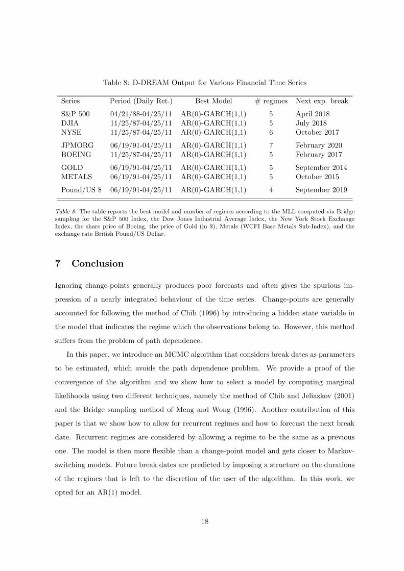
Table 8: D-DREAM Output for Various Financial Time Series

Series Period (Daily Ret.) Best Model # regimes Next exp. break

S&P 500 04/21/88-04/25/11 AR(0)-GARCH(1,1) 5 April 2018DJIA 11/25/87-04/25/11 AR(0)-GARCH(1,1) 5 July 2018NYSE 11/25/87-04/25/11 AR(0)-GARCH(1,1) 6 October 2017

JPMORG 06/19/91-04/25/11 AR(0)-GARCH(1,1) 7 February 2020BOEING 11/25/87-04/25/11 AR(0)-GARCH(1,1) 5 February 2017

GOLD 06/19/91-04/25/11 AR(0)-GARCH(1,1) 5 September 2014METALS 06/19/91-04/25/11 AR(0)-GARCH(1,1) 5 October 2015

Pound/US $ 06/19/91-04/25/11 AR(0)-GARCH(1,1) 4 September 2019

Table 8. The table reports the best model and number of regimes according to the MLL computed via Bridgesampling for the S&P 500 Index, the Dow Jones Industrial Average Index, the New York Stock ExchangeIndex, the share price of Boeing, the price of Gold (in $), Metals (WCFI Base Metals Sub-Index), and theexchange rate British Pound/US Dollar.

7 Conclusion

Ignoring change-points generally produces poor forecasts and often gives the spurious im-

pression of a nearly integrated behaviour of the time series. Change-points are generally

accounted for following the method of Chib (1996) by introducing a hidden state variable in

the model that indicates the regime which the observations belong to. However, this method

suffers from the problem of path dependence.

In this paper, we introduce an MCMC algorithm that considers break dates as parameters

to be estimated, which avoids the path dependence problem. We provide a proof of the

convergence of the algorithm and we show how to select a model by computing marginal

likelihoods using two different techniques, namely the method of Chib and Jeliazkov (2001)

and the Bridge sampling method of Meng and Wong (1996). Another contribution of this

paper is that we show how to allow for recurrent regimes and how to forecast the next break

date. Recurrent regimes are considered by allowing a regime to be the same as a previous

one. The model is then more flexible than a change-point model and gets closer to Markov-

switching models. Future break dates are predicted by imposing a structure on the durations

of the regimes that is left to the discretion of the user of the algorithm. In this work, we

opted for an AR(1) model.

18

We illustrate the efficiency and rapidity of the algorithm by means of simulations and

apply it to financial time series to highlight the presence of structural breaks. Indeed, all

eight series studied exhibit at least three structural breaks. In particular, we find evidence

of four structural breaks in the daily series of returns of the S&P 500 index at the following

dates: December 30, 1991, November 27, 1996, March 14, 2003, and January 17, 2007.

Further research could focus on applying the same type of algorithm to multivariate time

series. It is also of great importance to check whether detecting and forecasting structural

breaks really enhances the predictions or not. An ambitious research work would also focus

on the causes of structural breaks.

Appendix

Proof of Theorem 1

The proof is due to Vrugt, ter Braak, Diks, Robinson, Hyman, and Higdon (2009) and requires

minor adjustments in the present case. It consists of four steps and is based on the fact that

the chains do not converge separately of each other but rather converge together towards a

stationary distribution. In the first step, we recall the conditional detailed balance condition

required for the existence of a stationary distribution in a N-component Metropolis algorithm.

In the second step, we prove the conditional detailed balance of the D-DREAM algorithm. In

the third step, we show that the joint distribution of the break date vectors of the N chains

is the product of the marginal distributions of each vector of break dates. In the fourth step,

we prove the ergodicity of the chains and uniqueness of the stationary distribution. We give

here the proof for the Γ-block only.

• Step 1. Recalling conditional detailed balance.

In order to have the stationary distribution as target distribution one needs to show

that if (Γ(t)1 , ...,Γ

(t)N ) ∼ π̃(.), with π̃(.) the joint pdf of (Γ1, ...,ΓN ) at iteration t, then

(Γ(t+1)1 , ...,Γ

(t+1)N ) ∼ π̃(.) at iteration t+ 1. That is, one needs the conditional detailed

balance condition to be satisfied for each and every chain i such that, ∀i (omitting Θi

from the conditioning variables):

π̃(Γ(t)i |Γ

(t+1)1 , ...,Γ

(t+1)i−1 ,Γ

(t)i+1, ...,Γ

(t)N )×Ki(Γ

(t+1)i |Γ(t+1)

1 , ...,Γ(t+1)i−1 ,Γ

(t)i ,Γ

(t)i+1, ...,Γ

(t)N )

= π̃(Γ(t+1)i |Γ(t+1)

1 , ...,Γ(t+1)i−1 ,Γ

(t)i+1, ...,Γ

(t)N )×Ki(Γ

(t)i |Γ

(t+1)1 , ...,Γ

(t+1)i−1 ,Γ

(t+1)i ,Γ

(t)i+1, ...,Γ

(t)N ),

19

with Ki(.|.) the jumping kernel.

• Step 2. Proving the conditional detailed balance condition.

Now, we show that the D-DREAM algorithm for the Γi-block satisfies the detailed

balance condition with respect to π(.) such that:

π(Γ(t)i )Ki(Γ

(t+1)i |Γ(t+1)

1 , ...,Γ(t+1)i−1 ,Γ

(t)i ,Γ

(t)i+1, ...,Γ

(t)N )

= π(Γ(t+1)i )Ki(Γ

(t)i |Γ

(t+1)1 , ...,Γ

(t+1)i−1 ,Γ

(t+1)i ,Γ

(t)i+1, ...,Γ

(t)N ).

Recall that the proposal Zi for an update of chain i proceeds by random selection of

pairs of other chains. Hence, the kernel of this update is a mixture of kernels which

maintains conditional detailed balance with respect to π(.) if each of its components

does. Since ε follows a symmetric distribution and the pairs {∑δ

g=1 Γr1(g),∑δ

h=1 Γr2(h)}

and {∑δ

h=1 Γr1(h),∑δ

g=1 Γr2(g)} are equally likely, this condition is fulfilled by accepting

the proposal with probability min{f(YT |Zi)p(Zi)f(YT |Γ)p(Γ) ,1}. This also holds true with the round[.]

operator since it does not alter the symmetry of the proposal distribution and with the

binomial cross-over scheme used to modify only selected dimensions of Γi.9 10

• Step 3. Showing that the joint is the product of the marginals.

As showed in step 2, the kernel Ki(.|.) for updating chain i satisfies the detailed balance

condition of step 1 with, ∀i = 1, ...N , π̃(Γ(t)i |Γ

(t+1)1 , ...,Γ

(t+1)i−1 ,Γ

(t)i+1, ...,Γ

(t)N ) = π(Γ

(t)i ).

Since the identity in step 1 is satisfied with the marginal distribution π(Γ(t)i ), the D-

DREAM algorithm is an N-component Metropolis-within-Gibbs algorithm with joint

stationary distribution π̃(Γ1, ...,ΓN ), such that

π̃(Γ1, ...,ΓN ) = π(Γ1)× ...× π(ΓN ).

• Step 4. Proving ergodicity and uniqueness.

For ergodicity, it is sufficient to show that the chains are aperiodic because of the

9As discussed above, the two possible issues in the proposal - that a break date falls outside the samplelength [2,T] or that two break dates are inverted - are discarded by our prior distribution choice since thelikelihood of the proposal Zi would then be equal to zero.

10The round[.] operator must insure the symmetry for every possibilities. Hence a stochastic rounding hasto be implemented for a particular case where one of the proposal parameter has exactly a fractional partequal to .5 even though it will virtually never happen in practice.

20

discreteness of Γ. The condition is satisfied thanks to the random walk component

generated by ε in proposal 2. For uniqueness of the stationary distribution, it is sufficient

to show that the chains are irreducible which is guaranteed by the unbounded support

of the distribution of ε that necessarily covers the entire support [0,T].

Proposal Distribution for the Computation of the Marginal Likelihood via

Bridge Sampling

We consider independence between Θ and Γ. Following Ardia, Hoogerheide, and van Dijk

(2009) we work with a mixture of distributions. The proposal q(Θ) samples from a mixture of

five normally distributed components. The means of the first three components are set to the

posterior mean (mupm) of the MCMC draws and the most likely draw (µmax) of the MCMC

scheme defines the means of the last two components. The variance-covariance matrices of

all components differ from the variance-covariance matrix of the MCMC draws by a scaling

factor. The proposal q(Γ) consists of a two-component mixture and follows the same ideas as

for q(Θ). The weights were chosen arbitrarily. The information is summarized in table 9.

Table 9: Proposal Distribution Mixture

AR/GARCH parameters Γ parametersComp. # Weight Distribution Comp. # Weight Distribution

1 0.50 N(µpm,Σ) 1 0.75 N(µpm,0.01Σ)2 0.25 N(µpm,0.25Σ) 2 0.25 N(µpm,4Σ)3 0.10 N(µpm,10Σ)4 0.05 N(µmax,10Σ)5 0.10 N(µmax,Σ)

Table 9. The table shows the components in the proposal mixture used for the computation of the MLL viaBridge sampling. µpm and µmax stand respectively for the posterior mean of the MCMC draws and the mostlikely draw. Σ is the variance-covariance matrix obtained from the MCMC draws.

References

Amado, C., and T. Terasvirta (2008): “Modelling Conditional and Unconditional Het-

eroskedasticity with Smoothly Time-Varying Structure,” CREATES Research Papers 2008-

08, University of Aarhus.

21

Ardia, D., L. Hoogerheide, and H. van Dijk (2009): “AdMit : Adaptive Mixtures of

Student-t Distributions,” The R Journal, 1, 25–30.

Bauwens, L., A. Dufays, and J. V. K. Rombouts (2011): “Marginal Likelihood for

Markov-switching and Change-Point GARCH Models,” CORE discussion paper, 2011/13.

Bauwens, L., M. Lubrano, and J. Richard (1999): Bayesian Inference in Dynamic

Econometric Models. Oxford University Press, Oxford.

Bauwens, L., A. Preminger, and J. Rombouts (2010): “Theory and Inference for a

Markov-switching GARCH Model,” Econometrics Journal, 13, 218–244.

Bollerslev, T. (1986): “Generalized Autoregressive Conditional Heteroskedasticity,” Jour-

nal of Econometrics, 31, 307–327.

Chib, S. (1996): “Calculating Posterior Distributions and Modal Estimates in Markov Mix-

ture Models,” Journal of Econometrics, 75, 79–97.

Chib, S., and I. Jeliazkov (2001): “Marginal Likelihood from the Metropolis-Hastings

Output,” Journal of the American Statistical Association, 96, 270–281.

Diebold, F. (1986): “Comment on Modeling the Persistence of Conditional Variances,”

Econometric Reviews, 5, 51–56.

Engle, R. (1982): “Autoregressive Conditional Heteroscedasticity with Estimates of the

Variance of United Kingdom Inflation,” Econometrica, 50, 987–1007.

Engle, R., and J. Rangel (2008): “The Spline-GARCH Model for Low-Frequency Volatil-

ity and its Global Macroeconomic Causes,” Review of Financial Studies, 21, 1187–1222.

Fruhwirth-Schnatter, S. (2004): “Estimating Marginal Likelihoods for Mixture and

Markov-switching Models Using Bridge Sampling Techniques,” Econometrics Journal, 7,

143–167.

Gelman, A., and D. Rubin (1992): “Inference from Iterative Simulation Using Multiple

Sequences,” Statistical Science, 7, 457–472.

Gray, S. (1996): “Modeling the Conditional Distribution of Interest Rates as a Regime-

Switching Process,” Journal of Financial Economics, 42, 27–62.

22

Haas, M., S. Mittnik, and M. Paolella (2004): “Mixed Normal Conditional Het-

eroskedasticity,” Journal of Financial Econometrics, 2, 211–250.

He, Z., and J. Maheu (2010): “Real Time Detection of Structural Breaks in GARCH

Models,” Computational Statistics and Data Analysis, 54, 2628–2640.

Hillebrand, E. (2005): “Neglecting Parameter Changes in GARCH Models,” Journal of

Econometrics, 129, 121–138.

Lamoureux, C., and W. Lastrapes (1990): “Persistence in Variance, Structural Change,

and the GARCH Model,” Journal of Business and Economic Statistics, 8, 225–234.

Liao, W. (2008): “Bayesian Inference of Structural Breaks in Time Varying Volatility Mod-

els,” Working paper, New-York University.

Meng, X., and S. Schilling (2002): “Warp Bridge Sampling,” Journal of Computational

and Graphical Statistics, 11, 552–586.

Meng, X.-L., and W. Wong (1996): “Simulating Ratios of Normalizing Constants via a

Simple Identity : A theoretical Exploration,” Statistica Sinica, 6, 831–860.

Mira, A., and G. Nicholls (2004): “Bridge Estimation of the Probability Density at a

Point,” Statistica Sinica, 14, 603–612.

Pesaran, M. H., D. Pettenuzzo, and A. Timmermann (2006): “Forecasting Time Series

Subject to Multiple Structural Breaks,” Review of Economic Studies, 73, 1057–1084.

ter Braak, C. J. F., and J. A. Vrugt (2008): “Differential Evolution Markov Chain

With Snooker Updater and Fewer Chains,” Statistics and Computing, 18, 435–446.

Vrugt, J. A., C. J. F. ter Braak, C. G. H. Diks, B. A. Robinson, J. M. Hyman, and

D. Higdon (2009): “Accelerating Markov Chain Monte Carlo Simulation by Differential

Evolution with Self-Adaptative Randomized Subspace Sampling,” International Journal of

Nonlinear Sciences and Numerical Simulations, 10, 271–288.

23

Recent titles CORE Discussion Papers

2011/12. Jacques-François THISSE. Geographical economics: a historical perspective. 2011/13. Luc BAUWENS, Arnaud DUFAYS and Jeroen V.K. ROMBOUTS. Marginal likelihood for

Markov-switching and change-point GARCH models. 2011/14. Gilles GRANDJEAN. Risk-sharing networks and farsighted stability. 2011/15. Pedro CANTOS-SANCHEZ, Rafael MONER-COLONQUES, José J. SEMPERE-MONERRIS

and Oscar ALVAREZ-SANJAIME. Vertical integration and exclusivities in maritime freight transport.

2011/16. Géraldine STRACK, Bernard FORTZ, Fouad RIANE and Mathieu VAN VYVE. Comparison of heuristic procedures for an integrated model for production and distribution planning in an environment of shared resources.

2011/17. Juan A. MAÑEZ, Rafael MONER-COLONQUES, José J. SEMPERE-MONERRIS and Amparo URBANO Price differentials among brands in retail distribution: product quality and service quality.

2011/18. Pierre M. PICARD and Bruno VAN POTTELSBERGHE DE LA POTTERIE. Patent office governance and patent system quality.

2011/19. Emmanuelle AURIOL and Pierre M. PICARD. A theory of BOT concession contracts. 2011/20. Fred SCHROYEN. Attitudes towards income risk in the presence of quantity constraints. 2011/21. Dimitris KOROBILIS. Hierarchical shrinkage priors for dynamic regressions with many

predictors. 2011/22. Dimitris KOROBILIS. VAR forecasting using Bayesian variable selection. 2011/23. Marc FLEURBAEY and Stéphane ZUBER. Inequality aversion and separability in social risk

evaluation. 2011/24. Helmuth CREMER and Pierre PESTIEAU. Social long term care insurance and redistribution. 2011/25. Natali HRITONENKO and Yuri YATSENKO. Sustainable growth and modernization under

environmental hazard and adaptation. 2011/26. Marc FLEURBAEY and Erik SCHOKKAERT. Equity in health and health care. 2011/27. David DE LA CROIX and Axel GOSSERIES. The natalist bias of pollution control. 2011/28. Olivier DURAND-LASSERVE, Axel PIERRU and Yves SMEERS. Effects of the uncertainty

about global economic recovery on energy transition and CO2 price. 2011/29. Ana MAULEON, Elena MOLIS, Vincent J. VANNETELBOSCH and Wouter VERGOTE.

Absolutely stable roommate problems. 2011/30. Nicolas GILLIS and François GLINEUR. Accelerated multiplicative updates and hierarchical

als algorithms for nonnegative matrix factorization. 2011/31. Nguyen Thang DAO and Julio DAVILA. Implementing steady state efficiency in overlapping

generations economies with environmental externalities. 2011/32. Paul BELLEFLAMME, Thomas LAMBERT and Armin SCHWIENBACHER. Crowdfunding:

tapping the right crowd. 2011/33. Pierre PESTIEAU and Gregory PONTHIERE. Optimal fertility along the lifecycle. 2011/34. Joachim GAHUNGU and Yves SMEERS. Optimal time to invest when the price processes are

geometric Brownian motions. A tentative based on smooth fit. 2011/35. Joachim GAHUNGU and Yves SMEERS. Sufficient and necessary conditions for perpetual

multi-assets exchange options. 2011/36. Miguel A.G. BELMONTE, Gary KOOP and Dimitris KOROBILIS. Hierarchical shrinkage in

time-varying parameter models. 2011/37. Quentin BOTTON, Bernard FORTZ, Luis GOUVEIA and Michael POSS. Benders

decomposition for the hop-constrained survivable network design problem. 2011/38. J. Peter NEARY and Joe THARAKAN. International trade with endogenous mode of

competition in general equilibrium. 2011/39. Jean-François CAULIER, Ana MAULEON, Jose J. SEMPERE-MONERRIS and Vincent

VANNETELBOSCH. Stable and efficient coalitional networks.

Recent titles CORE Discussion Papers - continued

2011/40. Pierre M. PICARD and Tim WORRALL. Sustainable migration policies. 2011/41. Sébastien VAN BELLEGEM. Locally stationary volatility modelling. 2011/42. Dimitri PAOLINI, Pasquale PISTONE, Giuseppe PULINA and Martin ZAGLER. Tax treaties

and the allocation of taxing rights with developing countries. 2011/43. Marc FLEURBAEY and Erik SCHOKKAERT. Behavioral fair social choice. 2011/44. Joachim GAHUNGU and Yves SMEERS. A real options model for electricity capacity

expansion. 2011/45. Marie-Louise LEROUX and Pierre PESTIEAU. Social security and family support. 2011/46. Chiara CANTA. Efficiency, access and the mixed delivery of health care services. 2011/47. Jean J. GABSZEWICZ, Salome GVETADZE and Skerdilajda ZANAJ. Migrations, public

goods and taxes. 2011/48. Jean J. GABSZEWICZ and Joana RESENDE. Credence goods and product differentiation. 2011/49. Jean J. GABSZEWICZ, Tanguy VAN YPERSELE and Skerdilajda ZANAJ. Does the seller of

a house facing a large number of buyers always decrease its price when its first offer is rejected?

2011/50. Mathieu VAN VYVE. Linear prices for non-convex electricity markets: models and algorithms. 2011/51. Parkash CHANDER and Henry TULKENS. The Kyoto Protocol, the Copenhagen Accord, the

Cancun Agreements, and beyond: An economic and game theoretical exploration and interpretation.

2011/52. Fabian Y.R.P. BOCART and Christian HAFNER. Econometric analysis of volatile art markets. 2011/53. Philippe DE DONDER and Pierre PESTIEAU. Private, social and self insurance for long-term

care: a political economy analysis. 2011/54. Filippo L. CALCIANO. Oligopolistic competition with general complementarities. 2011/55. Luc BAUWENS, Arnaud DUFAYS and Bruno DE BACKER. Estimating and forecasting

structural breaks in financial time series.

Books J. HINDRIKS (ed.) (2008), Au-delà de Copernic: de la confusion au consensus ? Brussels, Academic and

Scientific Publishers. J-M. HURIOT and J-F. THISSE (eds) (2009), Economics of cities. Cambridge, Cambridge University Press. P. BELLEFLAMME and M. PEITZ (eds) (2010), Industrial organization: markets and strategies. Cambridge

University Press. M. JUNGER, Th. LIEBLING, D. NADDEF, G. NEMHAUSER, W. PULLEYBLANK, G. REINELT, G.

RINALDI and L. WOLSEY (eds) (2010), 50 years of integer programming, 1958-2008: from the early years to the state-of-the-art. Berlin Springer.

G. DURANTON, Ph. MARTIN, Th. MAYER and F. MAYNERIS (eds) (2010), The economics of clusters – Lessons from the French experience. Oxford University Press.

J. HINDRIKS and I. VAN DE CLOOT (eds) (2011), Notre pension en heritage. Itinera Institute. M. FLEURBAEY and F. MANIQUET (eds) (2011), A theory of fairness and social welfare. Cambridge

University Press. V. GINSBURGH and S. WEBER (eds) (2011), How many languages make sense? The economics of

linguistic diversity. Princeton University Press.

CORE Lecture Series D. BIENSTOCK (2001), Potential function methods for approximately solving linear programming

problems: theory and practice. R. AMIR (2002), Supermodularity and complementarity in economics. R. WEISMANTEL (2006), Lectures on mixed nonlinear programming.