Available online at www.sciencedirect.com

08) 123–132www.elsevier.com/locate/geoderma

Geoderma 143 (20

Inferences from fluctuations in the local variogram about theassumption of stationarity in the variance

R. Corstanje a,⁎, S. Grunwald b, R.M. Lark a

a Rothamsted Research, Harpenden, Hertfordshire, AL5 2JQ Great Britain, United Kingdomb Soil and Water Science Dep., University of Florida, FL 32611-0510, USA

Received 18 December 2006; received in revised form 11 July 2007; accepted 28 October 2007Available online 11 December 2007

Abstract

Geostatistics is commonly used to describe and predict the variation of soil properties over the landscape. However, many geostatisticalmethods require the assumption that our observed data are a realization of a random function which is intrinsically stationarity. Under stationarity,observations of a single realization of the random function at different positions can be treated as a form of replication. There are various ways inwhich a random function may breach the assumption of intrinsic stationarity and numerous geostatistical techniques have been developed that areable to cope with some forms of non-stationarity. What is currently needed is a set of diagnostic tools capable of detecting and identifying whendata cannot plausibly be treated as a realization of a process which is stationary in the variance.

In this paper, we propose an inferential method that can identify when stationarity in the variance cannot plausibly be assumed. The basis ofour approach is to obtain a model for the random function under the assumption of intrinsic stationarity. If the global dataset can be regarded as arealization of a Gaussian process (perhaps after transformation), then the global variogram is sufficient for this purpose. By using a window-basedmethod to locally estimate variograms, we can define some statistic of homogeneity of the sample variation of the data. This allows us to obtain asample distribution for this statistic, under the null hypothesis of intrinsic stationarity, by generating multiple realizations of the postulationrandom function at the original sample points using Monte Carlo methods and recomputing the statistic for each realization. We selected asstatistics the interquartile ranges of: i) the spatial dependence ratio (s), the proportion c1 / (c0+c1), ii) a distance parameter (a), which is themaximum lag over which the random function is autocorrelated for variograms like the spherical, and iii) the local variances (v; c0+c1), where (c0)is the nugget component and (c1) the spatially structured component. We demonstrated this method using data from the large scale sampling(n=1341 over 8248 km2) of the Florida Everglades, United States.Crown Copyright © 2007 Published by Elsevier B.V. All rights reserved.

Keywords: Soil; Geostatistics; Random processes; Stationarity; Spatial variation

1. Introduction

Soil-forming processes are very complex and our understandingof this complexity is imperfect. An effective way to treat thisuncertainty is to model soil properties as realizations of a randomfunction (Webster, 2000). Geostatistics generates models of theserandom functions, which are then used to describe variation in soilproperties at different spatial resolutions and can be used to predictthem at unsampled locations. This approach has been successfullyapplied to a wide range of soil properties, including soil metals(Goovaerts and Webster, 1994) and the composition of soil

⁎ Corresponding author.E-mail address: ron.corstanje@bbsrc.ac.uk (R. Corstanje).

0016-7061/$ - see front matter. Crown Copyright © 2007 Published by Elsevier Bdoi:10.1016/j.geoderma.2007.10.021

microbial communities (Brockman and Murray, 1997; Franklinand Mills, 2003) and various other soil properties (Grunwald,2006). Predictions from geostatistical models can often form theunderlying data used in precision farming (Sadler et al., 1998) or inenvironmental fate and process models (Corwin et al., 1997). Thegeostatistical model of spatial variation also underlies linear mixedmodels for spatial data (e.g. Lark and Cullis, 2004).

The principal underlying assumption of geostatistics is that thestochastic process is stationary. Consider a set of N samplinglocations along a line (transect), X=[x1,…, xN], then the dataobtained at these locations, z(x1),…, z(xN), are samples from themarginal distributions, D1,…, DN, which are projections of theN-variate distribution D of the random function Z(x). We haveonly one sample from each marginal distribution DN, resulting in

.V. All rights reserved.

124 R. Corstanje et al. / Geoderma 143 (2008) 123–132

one vector z(X)=z(x1),…, z(xN), drawn from D, which is insuf-ficient to estimate the parameters of D. In geostatistics we makeinferences about the random function Z(x) by invoking theassumption of stationarity. Under stationarity, the multiple obser-vations z(x1),…, z(xN) provide a kind of replication, i.e., any pair ofobservations z(xi), z(xi+h) are drawn from a bivariate process withthe same distribution. This assumption allows us to infer infor-mation about D and ultimately model the random function Z(x).

The assumption of stationarity in itsmost general sense impliesthat the joint distribution of the random function at all locationsdoes not depend on the absolute geographic location of the pointsamples, i.e. the models of spatially dependent variance(covariance structures) are the same over the entire sampledarea. Formally, when a random function is strictly stationary, thejoint distribution function at a set of N sample points, x1,…, xN, isinvariant when the origin of x1,…, xN is translated. As we discussbelow, the strict assumption of stationarity is not necessary ingeostatistics, but a minimal assumption of stationarity in themean(zero) and variance of the increments z(xi)−z(xi+h) is required.

The less serious breach of this assumption is a non-stationarymean, which can effectively be dealt with by using generalizedcovariances (Matheron, 1973) or the empirical best linear unbiasedpredictor with appropriate fixed effects (e.g., universal kriging;Meul and Van Meirvenne, 2003). A more serious violation of thisassumption is when the variance is non-stationary and this is thefocus of this paper. Non-stationary variance can take two forms, thevariancemay change as a function of space, i.e. the local variance ofa soil property changes at different locations.A second formof non-stationary variance occurs when the distribution of the variancebetween scales (or spatial frequencies) changes in space. Thesechanges in the scale-dependent distribution of variance imply achange in the autocorrelation function. Furthermore, variability ofsoil processes maywell be non-stationary as a consequence of bothchanges in the variance and in the autocorrelation function.

It is easy to conceive of spatial processes in which it is notplausible to assume that the underlying covariance structures arestationary over the scales of interest. For example, pollutiondispersion models in soils depend on certain characteristic soilproperties such as texture, which can govern contaminant sorptionor movement in the soil media. If empirical spatial covariances orempirical variograms are used to estimate texture across a landscapecharacterised by alluvial and glacial deposits as well as areas whereerosion is prevalent, the assumption of an underlying randomfunctionwhich is stationary in the variance is implausible because ofchanges in local variation of texture. Consider measurements of soilcarbon content on a transect that covers different parent materials,land use and vegetation. The characteristic spatial scales of variationin soil carbon content of clay soils under forestry may be largelydetermined by the structure of the forest canopy and managementunits for silvicultural production. If the transect also passes through arapidly changing ecotone, from forest to wetland to grassland, thenthe pattern of variation in SOC may be of a larger range than in thewoodland in this region of the transect, but with an important short-range pattern in the wetland, reflecting carbon ‘hot spots’ due tomicrotopographic variation. If we compute a variogram for thewhole transect, we assume, implausibly, that all this variation can betreated as a realization of a single stationary random function. In fact,

the variogram does not represent the variation in SOC anywhere inthe forest because the variability changes so markedly. Otherexamples where stationaritymight be implausible are given by Lark(2006) and Sampson and Guttorp (1992).

The simplest approach to address changing variances is topartition the sampling region into segments within which sta-tionarity is a more reasonable assumption (McBratney et al.,1991). There are also more complex techniques that can manageboth forms of non-stationary variances, e.g. deformation of theoriginal rectilinear coordinate space to obtain an alternative spacein which stationarity is plausible (Sampson and Guttorp, 1992).

Currently the practitioner must infer where stationaritycannot plausibly be assumed by either observing directionalvariogram behaviour (possibly after removing a trend), bycomparing variograms from portions of the sampling area orbased on some underlying knowledge about the variable andprocesses being modelled. This could be facilitated by methodsto test the plausibility of an underlying stationarity randomfunction, and to identify how this assumption appears to fail.Lark (2007) showed that it is possible to test the assumption ofstationarity in variance using the discrete wavelet transform andFuentes (2005) derived a spectral based test for stationarity.However, the wavelet tests require that the data is obtained froma uniform sampling on a square grid or transect, which is not themost efficient approach to estimating the variogram.

We probably cannot assume that many soil properties are arealization of a stationary random function because the varianceand/or the autocorrelation function appear to change. It is alsothe case that geostatistical methods that rely on the assumptionof stationarity are increasingly being used in soil science and thatmethods exist that can alleviate some of the effects of non-stationarity. However, there are currently few approaches to testfor non-stationarity of spatial processes. In this paper, we pro-pose an inferential method to test the plausibility of assumptionsof stationarity in the variance given that the underlying model isa random function. The method tests for changes in the varianceand autocorrelations.

2. Theory

Given the random function Z(x), strong stationarity occurswhen at any finite number of points x1,…, xN, the joint distributionof Z(x1),…, Z(xN) is the same as that of Z(x1+h),…, Z(xN+h)where h is some displacement. Aweaker formof stationarity is theassumption that a covariance function, Cov[Z (x+h), Z(x)] existsand depends only on h (equivalent to stationarity of the mean andvariance only). This form of stationarity is known as second orderstationarity. A still weaker form of the stationarity assumptionwas proposed by Matheron (1971, 1973). If the assumption ofstationarity is made, not about the random function Z(x) but aboutthe first order differences, Z(x+h)−Z(x), then this form ofstationarity is known as the intrinsic hypothesis.

Under the intrinsic hypothesis, Z(x) is stationary if;

(i) E[Z(x+h)−Z(x)]=0, for all x and h,(ii) Var[Z (x+h)−Z(x)]=E{[Z(x+h)−Z(x)]2}=2γ(h), for all x

and depends only on hwhere γ(h) denotes the semivariance.

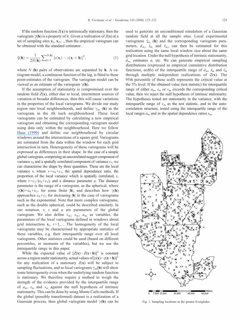
Fig. 1. Sampling locations in the greater Everglades.

125R. Corstanje et al. / Geoderma 143 (2008) 123–132

If the random function Z(x) is intrinsically stationary, then thevariogram γ(h) is a property of it. Given a realization of Z(x) at aset of sampling sites x1, x2,…, then the empirical variogram canbe obtained with the standard estimator:

g hð Þ ¼ 12N hð Þ

XN hð Þi¼1

z xið Þ � z xi þ hð Þ½ �2; ð1Þ

where N (h) pairs of observations are separated by h. A va-riogram model, a continuous function of the lag, is fitted to thesepoint-estimates of the variogram. The variogram model can beviewed as an estimate of the variogram γ(h).

If the assumption of stationarity is compromised over therandom field Z(x), either due to local, intermittent sources ofvariation or broader differences, then this will cause variationsin the properties of the local variograms. We divide our studyregion into local neighbourhoods, and define γmi

(h) as thevariogram in the ith such neighbourhood. These localvariograms can be estimated by calculating a new empiricalvariogram and obtaining the corresponding variogram modelusing data only within the neighbourhood. Here we followHaas (1990) and define our neighbourhood by circularwindows around the intersections of a square grid. Variogramsare estimated from the data within the window for each gridintersection in turn. Heterogeneity of these variograms will beexpressed as differences in their shape. In the case of a simpleglobal variogram, comprising an uncorrelated nugget component ofvariance c0 and a spatially correlated component of variance c1, wecan characterise the shape by three quantities. These are the localvariance v, where v=c0+c1, the spatial dependence ratio, theproportion of the local variance which is spatially correlated, s,where s=c1 / (c0+c1), and a distance parameter a. The distanceparameter is the range of a variogram, as the spherical, whereγ(h)=c0+c1, for some finite |h|, and describes how γ(h)approaches c0+ c1 for increasing |h| in the case of variogramssuch as the exponential. Note that more complex variograms,such as the double spherical, could be described similarly. Inour notation, v, s and a are parameters of the globalvariogram. We also define vmi

, smi, ami

as variables, theparameters of the local variograms defined in windows aboutgrid intersection xi, i=1,…. The homogeneity of the localvariograms may be characterised by appropriate statistics ofthese variables, e.g. their interquartile range over all localvariograms. Other statistics could be used (based on differentpercentiles, or moments of the variables), but we use theinterquartile range in this paper.

While the expected value of [Z(x)−Z(x+h)]2 is constantacross a region under stationarity, actual values of [z(x)−z(x+h)]2

for any realization of a stationary Z(x) will be subject tosampling fluctuations, and so local variograms γm(h) will showsome heterogeneity even when the underlying random functionis stationary. We therefore require a method to weigh thestrength of the evidence provided by the interquartile rangeof am, sm and vm against the null hypothesis of intrinsicstationarity. This can be done by usingMonte Carlo methods. Ifthe global (possibly transformed) dataset is a realization of aGaussian process, then global variogram model γ(h) can be

used to generate an unconditioned simulation of a Gaussianrandom field at all the sample sites. Local experimentalvariograms γmi

(h) and the corresponding variogram para-meters, ami

, smiand vmi

, can then be estimated for thisrealization using the same local window size about the samegrid location. Under the null hypothesis of intrinsic stationarity,ami

estimates a, etc. We can generate empirical samplingdistributions (expressed as empirical cumulative distributionfunctions, ecdfs) of the interquartile range of am, sm and vmthrough multiple independent realizations of Z(x). The95th percentile of these ecdfs represents the critical value atthe 5% level. If the obtained value (test statistic) for interquartilerange of either am, sm or vm exceeds the corresponding criticalvalue, then we reject the null hypothesis of intrinsic stationarity.The hypotheses tested are stationarity in the variance, with theinterquartile range of vm as the test statistic, and in the auto-correlation structure, tested using the interquartile range of thelocal ranges am and in the spatial dependence ratios sm.

126 R. Corstanje et al. / Geoderma 143 (2008) 123–132

3. Case study

We now illustrate the inference approach on four soil pro-perties from a large dataset at 1341 sites for a large area inSouthern Florida encompassing the Everglades National Park,Big Cypress National Preserve in the south and west and WaterConservation Areas (WCA) 1, 2, and 3 in the north (Fig. 1). Theentire extent of this area is 8248 km2. The soils in the northernareas are predominantly peat, the limestone bedrock tends to bemore influential on the soils towards the southern areas as thepeat layer becomes thinner. The plant communities in theEverglades show corresponding trends from north to south.Freshwater sawgrass marsh dominates the northern and centralareas, deepwater cypress swamp is predominant on the westernedges and the southern edges contain tidal salt marsh, andcoastal mangrove. The northern areas are characterised by aseries of nutrient gradients in response to a point source nutrientinfluxes (Newman et al., 1996, Bruland et al., 2006, Corstanjeet al., 2006, Rivero et al., 2007). The soils were sampledfollowing a stratified random sampling design (samplinglocations depicted in Fig. 1). Stratification was based onprevious soil sampling of the area (Newman et al., 1997) andhistoric ecological and hydrological data (Corstanje et al.,

Fig. 2. Frequency distributions and summary statistics of the variables used in this stuand calcium (Ca). Note that all variables are transformed to logarithms).

2006). Soil samples where taken to 10 cm depth throughout thearea. The soil properties measured included soil nutrient content(total nitrogen; TN, total phosphorus; TP, total inorganicphosphorus; TPi and total carbon), soil metals (Fe, Al, Mg,Ca) and basic soil properties such as bulk density and ashcontent. Current geostatistical analysis on this dataset has re-flected the hydrological units and boundaries within the systemand a significant amount of work has been accomplished inunderstanding and refining predictions within these units(Bruland et al., 2006, Corstanje et al., 2006, Rivero et al.,2007). The size and coverage of this dataset makes it suitable fora detailed study to test to what degree the assumption ofstationarity (second order stationarity) is realistic over such alandscape. We selected four properties; TP, TPi, Ca and TN, andlimited the analysis to the 0–10 cm depth interval as this was theonly layer with complete coverage. Descriptions of thelaboratory analysis are supplied in Bruland et al. (2006) andCorstanje et al. (2006), data provided with kind permission byDr Ramesh Reddy, Wetland Biogeochemistry Laboratory,University of Florida.

Possible sources of complex variation across this area thatwouldmake the stationarity assumption implausible might be found in thephosphorus forms (TP and TPi) due to the local (b5 km)

dy (total phosphorus (TP), total inorganic phosphorus (TPi), total nitrogen (TN)

Fig. 3. Global experimental variograms and fitted models for the properties total phosphorus (TP), total inorganic phosphorus (TPi), total nitrogen (TN) and calcium(Ca) in the soil.

Table 1Interquartile ranges of the local distance parameter am, variance vm and spatialdependence ratio sm and the 95th percentile obtained from the cumulativedistribution functions of the interquartile range of the local distance parameteram, variance vm and spatial dependence ratio sm over all moving windows of thesampling space

Soil property Interquartile range

Local statistic am vm sm

TP 19,426 0.13 0.15TPi 19,263 0.16 0.10TN 13,242 0.29 0.32CA 25,989 0.50 0.13

Critical value,95th percentile

am vm sm

TP 20,366 0.11 0.094TPi 8950 0.076 0.11TN 39,327 0.58 0.68CA 42,363 0.66 0.50

127R. Corstanje et al. / Geoderma 143 (2008) 123–132

enrichment gradients or in all four properties in response tovariation in depth to bedrock, with overlying heterogeneity in plantcommunities (e.g. ridges and sloughs, tree islands) or micro-topography.

As our method assumes normality (realizations of normalrandom variables are used in the Monte Carlo simulations) andthe distributions of all four properties were found to be skewed,we transformed all the data to natural logarithms. All analyseswere done on the transformed data. Fig. 2 shows frequencyhistograms for the transformed data including summarystatistics. The transformed data on TP and TPi are symme-trically distributed, the data on TN have a negative skew, andthe data on Ca show a small positive skew with a small secondmode in the upper tail. We then computed the globalexperimental variograms for the four properties (Fig. 3),selected the appropriate variogram models using the Akaikeinformation criterion (McBratney and Webster, 1989) andobtained the model parameters by weighted least squares. Allfour variograms show that there is spatially-autocorrelated vari-ability. The global ranges a of TP, TPi, TN and Ca wereestimated at 33, 45, 64, 36 km respectively. The respective total(sill) variances v were estimated at 0.49, 0.62, 0.65 and 1.34 andglobal spatial-dependent ratios s were estimated at 0.69, 0.45,0.83 and 0.72 for TP, TPi, TN and Ca respectively.

Local variogram parameters were subsequently estimatedusing a moving window. We selected the window size by

considering the number of sites available for the local variogramestimates while maintaining a minimum number of windowsrequired to obtain the estimates of the statistics of homogeneity.For this dataset, we chose a window radius of 30 km, the centreof which was sequentially placed on grid intersect points of a 10by 10 km grid. This resulted in 105 overlapping windows. Each

Fig. 4. Empirical cumulative distribution functions for three statistics of variogram homogeneity, the local distance parameter am, variance vm and spatial dependenceratio sm for total phosphorus (TP) and total inorganic phosphorus (TPi). The horizontal dotted line denotes 95%, the vertical dotted line denotes the 95th percentile.

128 R. Corstanje et al. / Geoderma 143 (2008) 123–132

window containing an average of 270 observations, the smallestnumber of observations in a single window was 100. Thestatistics of homogeneity consisted of the interquartile range of

Fig. 5. Empirical cumulative distribution functions for three statistics of variogram horatio sm for total nitrogen (TN) and total calcium (Ca). The horizontal dotted line de

the local ranges am, the spatial dependence ratios sm and thelocal variances vm over all 105 windows in the sampling space,these have been presented in Table 1 as the local statistics.

mogeneity, the local distance parameter am, variance vm and spatial dependencenotes 95%, the vertical dotted line denotes the 95th percentile.

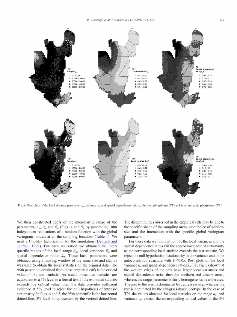
Fig. 6. Post plots of the local distance parameter am, variance vm and spatial dependence ratio sm for total phosphorus (TP) and total inorganic phosphorus (TPi).

129R. Corstanje et al. / Geoderma 143 (2008) 123–132

We then constructed ecdfs of the interquartile range of theparameters, am, sm and vm (Figs. 4 and 5) by generating 1000independent realizations of a random function with the globalvariogram models at all the sampling locations (Table 1). Weused a Cholsky factorization for the simulation (Deutsch andJournel, 1992). For each realization we obtained the inter-quartile ranges of the local range am, local variances vm andspatial dependence ratios sm. These local parameters wereobtained using a moving window of the same size and step aswas used to obtain the local statistics on the original data. The95th percentile obtained from these empirical cdfs is the criticalvalue of the test statistic. As noted, these test statistics areequivalent to a 5% level in a formal test. If the estimated statisticexceeds the critical value, then the data provides sufficientevidence at 5% level to reject the null hypothesis of intrinsicstationarity. In Figs. 4 and 5, the 95th percentile is the horizontaldotted line, 5% level is represented by the vertical dotted line.

The discontinuities observed in the empirical cdfs may be due tothe specific shape of the sampling areas, our choice of windowsize and the interaction with the specific global variogramparameters.

For these data we find that for TP, the local variances and thespatial dependence ratios fail the approximate test of stationarityas the corresponding local statistic exceeds the test statistic. Wereject the null hypothesis of stationarity in the variance and in theautocorrelation structure with Pb0.05. Post plots of the localvariance vm and spatial dependence ratios sm (TP, Fig. 6) show thatthe western edges of the area have larger local variances andspatial dependence ratios than the northern and eastern areas,whereas the range parameter is fairly homogeneous over the area.The area to the west is dominated by cypress swamp, whereas therest is dominated by the sawgrass marsh ecotype. In the case ofTPi, the values obtained for local statistics on the range am andvariance vm exceed the corresponding critical values at the 5%

Fig. 7. Post plots of the local distance parameter am, variance vm and spatial dependence ratio sm for total nitrogen (TN) and total calcium (Ca).

130 R. Corstanje et al. / Geoderma 143 (2008) 123–132

level.We therefore reject the null hypothesis that TPi is stationaryin the variance and in the autocorrelation structure. The localvariances vm for this property are larger toward the western edgesof the Everglades, coincidental with the forested, cypress do-minated areas (Fig. 6). The ranges observed for TPi were lower inthe north and western and southern edges of the area, but containslocal fluctuations throughout the area. We cannot reject the nullhypothesis of stationarity for all tests for the properties Ca and TN(Table 1). These properties can therefore be considered stationaryin their variance and autocorrelation structures over an area wheresome regional patterns in these properties are evident (Fig. 7).These two variables deviate most from a normal distribution(Fig. 2), which suggests that our test is not sensitive to thenormality assumption.

In terms of the soil processes that operate in the Everglades, apossible reason why Ca and TN conform to the stationaryassumption whereas TP and TPi do not, is that the variation in

the first two properties may be a function of the underlyinggeology (Ca) and still represent the connected peat system (TN)that existed in the original Everglades. Whereas the spatialvariation in the P forms seems more localized and a function ofmodern disturbances such as P inputs. There is no evidence ofany of major infrastructure components (e.g. roads, canals, etc.)in the figures of local variance, spatial dependence or range.This suggests that these may not have a great effect on spatialvariation in the four soil properties.

4. Discussion

Themethod proposed in this paper computes local estimates ofthe variogram parameters, within a moving window, and com-pares their variability with that of the corresponding variogramsfor a realization of a stationary random function with the sameglobal variogram as the real data. To our knowledge, it is one of a

131R. Corstanje et al. / Geoderma 143 (2008) 123–132

few approaches currently available to determine whether theassumption of intrinsic stationarity of the variance is appropriatefor a given set of data. The disadvantages of using moving win-dows are that they are computationally intensive for long rangeprocesses and the choice of thewindow size is somewhat arbitrary.The technique also requires fairly large datasets. The Bayesianspectral method developed by Fuentes (2005) generates similarinferences on non-stationary processes. It also requires somearbitrary decision because it is also a window-based approach andrequires the selection of a weight function. This is not the case inthe wavelet based approach presented by Lark (2006). However,the wavelet approach requires a dataset on a regular grid and maytherefore be more appropriate for exhaustively sampled soilproperties such as elevation or satellite imagery.

We have noted that our method is demanding of data.However, large datasets on easy-to-measure variables (com-monly from sensors) are now increasingly available in soilscience (e.g. including remote sensing (de Bruin, 2000), electro-magnetic induction (James et al., 2003), or yield monitoring(Dobermann and Ping, 2004). Our method may be of practicaluse in the analysis of such data. First, while densely sampled,these variables are often not regularly sampled and geostastis-tical methods may be needed to interpolate them, or to computeestimates at coarser scales by block kriging. These methodsassume stationarity. Second, if this assumption of stationarity isimplausible for an ancillary variable such as apparent electricalconductivity (ECa), then it is likely that it is implausible for arelated soil variable (e.g. clay content). Information on how thestationarity assumption appears to fail for ECa might be used toplan sampling of the soil (e.g. to insure adequate samplingwithin different regions within which the assumption ofstationarity is plausible). Finally, if the ancillary variable cannotbe plausibly assumed to be stationary in the variance this willcause problems if it is to be used for cokriging directmeasurements of a soil property. Again, in such circumstancesfield sampling of the soil might be planned so that thegeostatistical analysis can be carried out separately in differentsubregions.

If our test suggests that stationarity is an implausibleassumption, it will also indicate how this problem might betackled in subsequent analysis while we look separately at theplausibility of stationarity in different aspects of the variability.In the case where the spatial dependencies and ranges do notvary significantly but the variance does, then HierarchicalGeneralized Linear Models (Lee and Nelder, 2001) might besuitable. In this approach, the variance ismodelled as a function ofsome covariate(s). In the case where the variance seems to respondto localized perturbations, a robust estimator of the variogram(Lark, 2000) might mitigate the effects of local features ofvariation. Alternatively, if the variance changes as a result ofdistinct features in the landscape (such as the ecotypes cypressforest versus sawgrass marsh, or areas of high phosphorus soilcontent), then analysis could proceed by stratification for separateanalysis. In the case where spatial dependencies and ranges appearto be non-stationary, but the local variance does not, non-lineartransformations of coordinate systems (Sampson and Guttorp,1992) might be appropriate. This method obtains local deforma-

tions of the coordinate space, a nonlinear transformation of thecoordinate space to a spacewhere the spatial structure is stationary.Adaptations of this approach are increasingly being applied tospatial-temporal processes (see e.g., Schmidt andO'Hagan, 2003).Again, non-stationarity in the spatial dependence and/or rangemight be handled by stratification suggested by inspecting thelocal estimates of these parameters (e.g. our Fig. 6 or 7).

Acknowledgements

The authors would like to thank Dr Ramesh Reddy and theWetland Biogeochemistry Laboratory for providing us with thedata. This work was funded by the Biotechnology and BiologicalSciences Research Council under grant BB/C506813/1, andthrough its core grant to Rothamsted Research.

References

Brockman, F.J., Murray, C.J., 1997. Subsurface microbiological heterogeneity:current knowledge, descriptive approaches and applications. FEMSMicrobiol. Rev. 20, 231–247.

Bruland, G.L., Grunwald, S., Osborne, T.Z., Reddy, K.R., Newman, S., 2006.Spatial Distribution of soil properties in water conservation area 3 of theEverglades. Soil Sci. Soc. Am. J. 70, 1662–1676.

Corstanje, R., Grunwald, S., Reddy, K.R., Osborne, T.Z., Newman, S., 2006.Assessment of the spatial distribution of soil properties in a northern evergladesmarsh. J. Environ. Qual. 35, 938–949.

Corwin, D.L., Vaughan, P.J., Loague, K., 1997. Monitoring nonpoint sourcepollutants in the vadose zone with GIS. Environ. Sci. and Technol. 31,2157–2175.

de Bruin, S., 2000. Predicting the areal extent of land-cover types usingclassified imagery and geostatistics. Remote Sens. Environ. 74,387–396.

Deutsch, C.V., Journel, A.G., 1992. GSLIP: Geostatistical Software Library andUser's Guide. Oxford Univ. Press, New York, USA.

Dobermann, A., Ping, J.L., 2004. Geostatistical integration of yield monitor dataand remote sensing improves yield maps. Agron. J. 96, 285–297.

Franklin, R.B., Mills, A.L., 2003. Multiscale variation in spatial heterogeneityfor microbial community structure in an eastern Virginia agricultural field.FEMS Microbiol. Ecol. 44, 335–346.

Fuentes, M., 2005. A formal test for nonstationarity of spatial stochasticprocesses. J. Multivar. Stat. 96, 30–54.

Goovaerts, P., Webster, R., 1994. Scale-dependent correlation between topsoilcopper and cobalt concentrations in Scotland. Eur. J. Soil Sci. 45, 79–95.

Grunwald, S. (Ed.), 2006. Environmental Soil-LandscapeModeling. CRC press,Boca Raton, Florida, USA.

Haas, T.M., 1990. Lognormal and moving window methods of estimating aciddeposition. J. Am. Stat. Assoc. 85, 950–963.

James, I.T., Waine, T.W., Bradley, R.I., Taylor, J.C., Godwin, R.J., 2003.Determination of soil type boundaries using electromagnetic inductionscanning techniques. Biosys. Eng. 86, 421–430.

Lark, R.M., 2000. A comparison of some robust estimators of the variogram foruse in soil survey. Eur. J. Soil Sci. 51, 137–157.

Lark, R.M., 2006. Analysis of complex soil variation using wavelets. In:Grunwald, S. (Ed.), Environmental Soil-Landscape Modeling. CRC press,Boca Raton, Florida, USA, pp. 343–369.

Lark, R.M., 2007. Inference about soil variability from the structure of the bestwavelet packet basis. Eur. J. Soil Sci. 58, 822–831.

Lark, R.M., Cullis, B.R., 2004. Model-based analysis using REML forinference from systematically sampled data on soil. Eur. J. Soil Sci. 55,799–813.

Lee, Y., Nelder, J.A., 2001. Hierarchical generalised linear models: a synthesisof generalised linear models, random-effect models and structureddispersions. Biometrika 88, 987–1006.

132 R. Corstanje et al. / Geoderma 143 (2008) 123–132

Matheron, G., 1971. The theory of regionalized variables and its applications:Centre for Geostatistics. Fontainebleau. 212 p.

Matheron, G., 1973. The intrinsic random functions and their applications. Adv.in Appl. Prob. 5, 439–468.

McBratney, A.B., Hart, G.A., McGarry, D., 1991. The use of region partitioningto improve the representation of geostatistically mapped soil attributes. J.Soil Sci. 42, 513–532.

McBratney, A.B., Webster, R., 1989. On the Akaike information criterion forchoosing models for variograms of soil properties. J. Soil Sci. 40,493–496.

Meul, M., Van Meirvenne, M., 2003. Kriging soil texture under different typeson nonstationarity. Geoderma 112, 217–233.

Newman, S., Grace, J.B., Koebel, J.W., 1996. Effects of nutrients andhydroperiod on Typha, Cladium, and Eleocharis: implications for Ever-glades restoration. Ecol. Appl. 6, 774–783.

Newman, S., Reddy, K.R., DeBusk,W.F., Wang, Y., 1997. Spatial distribution ofsoil nutrients in a northern Everglades marsh: water conservation area 1. SoilSci. Soc. Am. J. 61, 1275–1283.

Rivero, R.G., Grunwald, S., Osborne, T.Z., Reddy, K.R., Newman, S., 2007.Characterization of the spatial distribution of soil properties in waterconservation area —2A, Everglades, Florida. Soil Sci. 172, 149–166.

Sadler, E.J., Busscher, W.J., Bauer, P.J., Karlen, D.L., 1998. Spatial scalerequirements for precision farming: a case study in the southeastern USA.Agron. J. 90, 191–197.

Sampson, P.D., Guttorp, P., 1992. Nonparametric estimation of nonstationaryspatial covariance structure. J. Am. Stat. Assoc. 87, 108–119.

Schmidt, A.M., O'Hagan, A., 2003. Bayesian inference for non-stationaryspatial covariance structure via spatial deformations. J. R. Stat. Soc. B 65,743–758.

Webster, R., 2000. Is soil variation random? Geoderma 97, 149–163.