The Consumer Rationality Assumption in Incentive Based Demand Response Program via Reduction Bidding

J Electr Eng Technol Vol. 10, No. ?: 742-?, 2014 http://dx.doi.org/10.5370/JEET.2015.10.?.742

742

The Consumer Rationality Assumption in Incentive Based Demand Response Program via Reduction Bidding

Muhammad Babar†, Imthias Ahamed T.P.* and Essam A. Alammar**

Abstract – Because of the burgeoning demand of the energy, the countries are finding sustainable solutions for these emerging challenges. Demand Side Management is playing a significant role in managing the demand with an aim to support the electrical grid during the peak hours. However, advancement in controls and communication technologies, the aggregators are appearing as a third party entity in implementing demand response program. In this paper, a detailed mathematical framework is discussed in which the aggregator acts as an energy service provider between the utility and the consumers, and facilitate the consumers to actively participate in demand side management by introducing the new concept of demand reduction bidding (DRB) under constrained direct load control. Paper also presented an algorithm for the proposed framework and demonstrated the efficacy of the algorithm by considering few case studies and concluded with simulation results and discussions. Keywords: Aggregator, Demand side management, Direct load control, Dynamic bidding, Dynamic programming

1. Introduction The advancements in information and communication

technology and burgeoning challenges in supply and demand of electrical power have led to the concept of Smart Grid [1]. Smart Grid is expected to improve the efficiency, quality, reliability, economics and sustainability of complete Supply and Demand chain of the Electricity [2]. In brief, Smart Grid is an energy management system of electrical power grid using advance data communication and networking in order to cope with skyrocketing demand and provide economic benefit to all stakeholders.

Demand Side Management is one of the most important management strategy in the Smart Grid paradigm that aims to balance electrical supply and demand by reducing the power demand during critical periods instead of increasing the power generation [3].

Researchers have identified significance of demand response in demand-side management program and consequently have presented many scheduling algorithms and formulated policies and strategies for demand-side management [4, 5]. It has been a crucial challenge to introduce various Demand Response (DR) programs in the electricity market and increase demand-side participation of the commercial as well as domestic consumers in electricity markets either through price signals or incentives, and carry out integrated resource planning (IRP) to

coordinate both supply-side and demand-side resources [6, 7]. Accordingly, DR programs could be generally classified into two basic categories: price-based DR and incentive-based DR [8].

Though, Incentive-based DR refers to the program in which consumers switch OFF their dispatchable loads to an event during a peak demand. Incentive-based DR usually include direct load control (DLC), interruptible/curtailable (I/C) service, demand bidding/buyback (DB), emergency demand response programs (EDRP), capacity market programs (CMP), and ancillary services market programs (ASMP). Moreover, Consumers participating in incentive based DR programs can either receive discounted retail rates or separate incentive payment against load reductions.

However, the implementation of Incentive-based direct load control (IB-DLC) program is very demanding for the utility because in this program the utility has to directly

† Corresponding Author: Electrical Energy Systems Group, Depart-ment of Electrical Engineering, Technology University of Eindhoven, The Netherlands. ([email protected])

* Department of Electrical and Computer Engineering, College of Engineering, Dhofar University, Salalah, Sultanate of Oman.

** Saudi Aramco Chair in Electrical Power, Department of Electrical Engineering, King Saud University, Riaydh, Saudi Arabia.

Received: June 4, 2013; Accepted: September 4, 2014

ISSN(Print) 1975-0102 ISSN(Online) 2093-7423

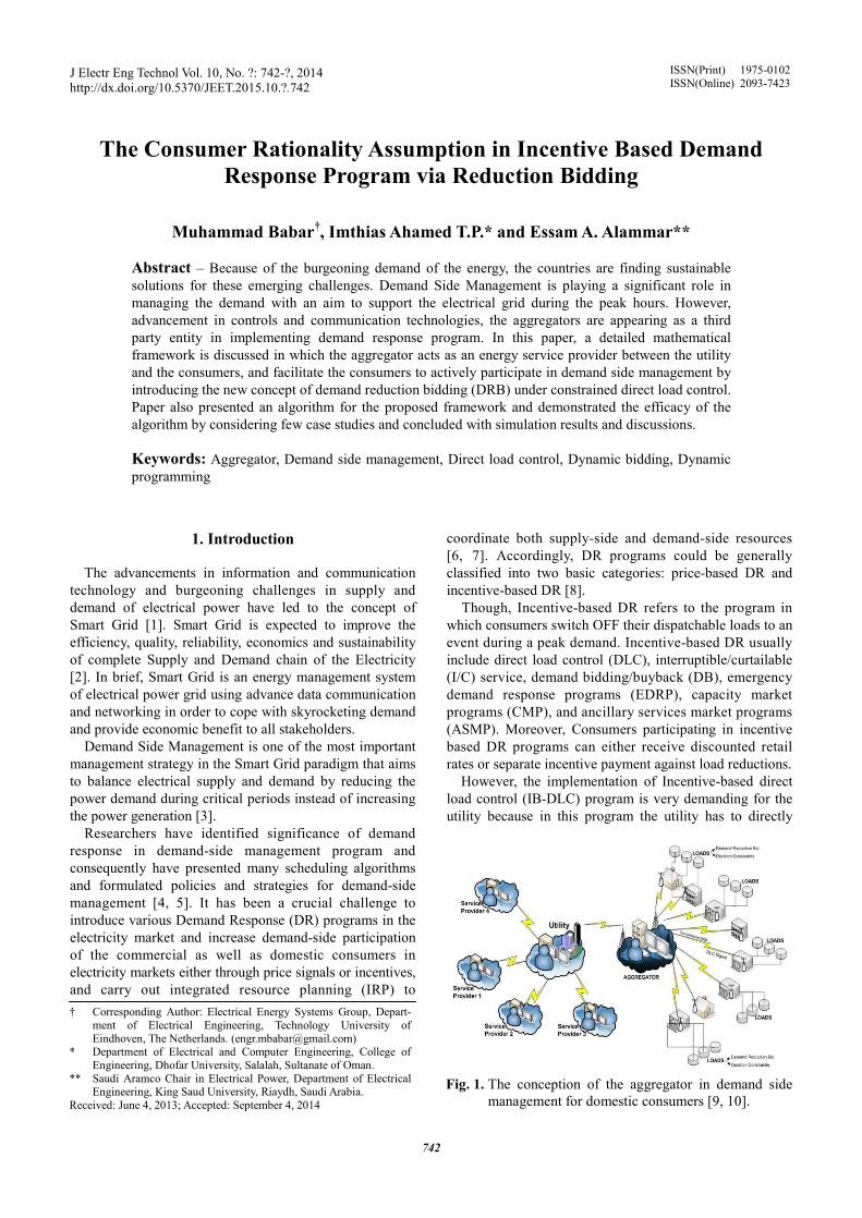
Fig. 1. The conception of the aggregator in demand side

management for domestic consumers [9, 10].

Muhammad Babar, Imthias Ahamed T.P.

communicate and control the thousands of consumers at an event during the peak period. Therefore, in the current emerging electricity market, new third party business entity is introduced which implements IBfor the utility. Till today, there is no precise definition for these third party entities but they are generally known as “Energy service provider” or the “Aggregators” between the utility and the consumers as shown in Fig. 1. The energy service providers and the utility usually has ”directed interaction” which means the utthe service provider that it has to curtail certain power through direct load controlling of the dispatchable loads of the participating consumers whenever it requires. For this service, it would be rewarded by the utility [11, 12].

Moreover, it could be noted that the utility usually want to reduce the bulk of power during peak hours and it is normally not in the capacity of any individual service provider. So, the utility signs an agreement with number of service providers and sees them as a large consumers as shown in Fig. 1. Accordingly, each service provider have an objective to shave the peak demand and support the utility in supplying uninterrupted and high quality power to commercial, industrial, institutional and domestic as well as electric vehicles during peak hours with ancillary services [13]. For reference, PG&E has started nonprogram named “Aggregator Managed Portfolio program” according to which it signs bilateral contracts with service providers by which it may call power curtailment events during high-price periods, emergencies and tests with price-responsive pricing mechanism [14].

Besides all, it has been an issue for the service provider to attract the consumers for IB-DLC program and retain them. Therefore, lot of effort has been made by the service providers in order to attract and motivate the consumers such that they allow the service provider to directly control their dispatchable loads during the peak hours [15

In short, in this paper, innovative framework fincentive based DR program is designed which enables consumers to directly interact with energy market by bidding against their power curtailment as well as effectively satisfy the consumer by considering their defined constraints. These constraints incratings of the dispatchable loads, price bids corresponding to each dispatchable load, maximum time allowed for control, the minimal time required between two consecutivecontrols and total control period of each dispatchable load of every consumer. Thus, the implementation of incentive based control program with these “consumer constraints” will attract a large number of consumers to perform IBDLC program and gain full benefit from it without altering their life style and personal space. In addition, a design of the proposed framework will also help the service provider in achieving the Win-Win situation i.e. maximize its own revenue, minimize utility’s operational cost by shaving the demand peak and satisfy the consumers through “consumer constraints”.

1 2{ , ,..., ,..., }n n n n nd Dp p p p=R

1 2{ , ,..., ,..., }n n n n nd Dq q q q=Q

Muhammad Babar, Imthias Ahamed T.P. and Essam A. Alammar

743

nds of consumers at event during the peak period. Therefore, in the current

emerging electricity market, new third party business entity is introduced which implements IB-DLC program for the utility. Till today, there is no precise definition

third party entities but they are generally “Energy service provider” or the “Aggregators”

between the utility and the consumers as shown in Fig. 1. The energy service providers and the utility usually has ”directed interaction” which means the utility directs the service provider that it has to curtail certain power through direct load controlling of the dispatchable loads of the participating consumers whenever it requires. For

service, it would be rewarded by the utility [11, 12]. it could be noted that the utility usually

want to reduce the bulk of power during peak hours and normally not in the capacity of any individual service

provider. So, the utility signs an agreement with number of large consumers as

shown in Fig. 1. Accordingly, each service provider have an objective to shave the peak demand and support the utility in supplying uninterrupted and high quality power to commercial, industrial, institutional and domestic as

ectric vehicles during peak hours with ancillary services [13]. For reference, PG&E has started non-tariff program named “Aggregator Managed Portfolio program” according to which it signs bilateral contracts with service

r curtailment events price periods, emergencies and tests with

Besides all, it has been an issue for the service provider

DLC program and retain fort has been made by the service

providers in order to attract and motivate the consumers such that they allow the service provider to directly control their dispatchable loads during the peak hours [15-18].

In short, in this paper, innovative framework for incentive based DR program is designed which enables consumers to directly interact with energy market by bidding against their power curtailment as well as effectively satisfy the consumer by considering their defined constraints. These constraints include the power ratings of the dispatchable loads, price bids corresponding to each dispatchable load, maximum time allowed for control, the minimal time required between two consecutive controls and total control period of each dispatchable load

onsumer. Thus, the implementation of incentive based control program with these “consumer constraints” will attract a large number of consumers to perform IB-DLC program and gain full benefit from it without altering

addition, a design of the proposed framework will also help the service provider

Win situation i.e. maximize its own revenue, minimize utility’s operational cost by shaving the demand peak and satisfy the consumers through “consumer

This also paper presents an algorithm for the service provider which generates a Consolidated Demand Reduction Bid (CDRB) which support it in materializing the concept of IB-DLC program with “energy bidding” at consumer level and help in obtairest of the paper structured as follows. Section 2 presents the proposed framework in detail and introduces the complete concept of CDRB. Section 3 formulates and develops the proposed algorithm which by using “Multiple Decision Making Problem (MDMP)”. Section 4 presents the simulation results to discuss the applicability of the framework and efficacy of the algorithm in the light of three scenarios. Finally, section 5 concludes the paper.

2. Design of the Framework Assume there are N number of consumers which are in

contract with the service provider and agreed to participate in the DRB based incentive program. For instance, assume any nth consumer out of N consumers which has identified D loads having ratings 1 2{ , ,..., ,..., }n n n n n

d Dp p p p=RMoreover, in this framework which presents the demand

reduction bid based incentive program for consumers, where consumer also identifies bids to decommit each dispatchable load during a control interval |H| which is denoted by Qn. However, these bids for each load are referred as Ex-ante bids which mean these bids are mutually decided by the consumer and the service provider at the time of agreement. Because, the service provider has to ex-ante validate these bids which means the bidsconsumers should be within the price limits specified by the service provider. Depending on the importance of each load, user specifies 1 2{ , ,..., ,..., }n n n n n

d Dq q q q=Qother hand, over expected load utilization and curtailment capability of every dispatchable load, the consumer also provide “duration constraints” that are

T

i.e. the set of minimum durations for which each load of nconsumer must be ON continuously,

T ,

i.e. the set of maximum duration for which each load could be OFF continuously and

T

i.e. the set total durations for which each load of nth consumer can participate in load reduction such that:

Thus, Qn and Rn are referred as load parameters and

This also paper presents an algorithm for the service provider which generates a Consolidated Demand Reduction Bid (CDRB) which support it in materializing

DLC program with “energy bidding” at consumer level and help in obtaining the full benefits. The rest of the paper structured as follows. Section 2 presents the proposed framework in detail and introduces the complete concept of CDRB. Section 3 formulates and develops the proposed algorithm which by using “Multiple

Making Problem (MDMP)”. Section 4 presents the simulation results to discuss the applicability of the framework and efficacy of the algorithm in the light of three scenarios. Finally, section 5 concludes the paper.

Design of the Framework

Assume there are N number of consumers which are in contract with the service provider and agreed to participate in the DRB based incentive program. For instance, assume any nth consumer out of N consumers which has identified

1 2{ , ,..., ,..., }n n n n nd Dp p p p=R .

Moreover, in this framework which presents the demand reduction bid based incentive program for consumers, where consumer also identifies bids to decommit each dispatchable load during a control interval |H| which is

wever, these bids for each load are ante bids which mean these bids are

mutually decided by the consumer and the service provider at the time of agreement. Because, the service provider has

ante validate these bids which means the bids by the consumers should be within the price limits specified by the service provider. Depending on the importance of each

1 2{ , ,..., ,..., }n n n n nd Dq q q q=Q . On the

other hand, over expected load utilization and curtailment y dispatchable load, the consumer also

provide “duration constraints” that are

i.e. the set of minimum durations for which each load of nth consumer must be ON continuously,

,...,

i.e. the set of maximum duration for which each load could

i.e. the set total durations for which each load of nth consumer can participate in load reduction such that:

are referred as load parameters and

The Consumer Rationality Assumption in

,mixn

ONT maxnOFFT and maxnT are referred as duration

constraints defined by the consumer to the service provider for all the dispatchable loads at the time of the agreement. The consideration of load parameters by the service provider in its demand response program will motivate theconsumers to participate as well as it help in portraying consumer’s “Desire of Use”. In addition, the given duration constraints with load parameters will also help the consumers in completely translating their needs and wants. In this proposed framework, load parameters and duration constraints will be collectively referred as Consumer Constraints and represented as:

For an explanation of the consumer constraints, assume

an example of a consumer who signed an agreement with the service provider for 6 dispatchable loads i.e. {d3, d4, d5, d6} and at the time of deal, consumer has identified load parameters and duration constraints as shown in Table 1. So, it can also be observed from Table 1 that consumer depending on his/her “Desire of Use” bid highest to d2 and bid least to d5. In addition, it can also observed that the maximum OFF time for the load d2 is merely 0.5 hours which signifies its importance to the consumer. d2 also has a significantly greater continuous ON time as compared to other loads while the total maximum OFF time is only 30 mins i.e. the service provider can only turn it OFF for just 30 mins in a day. As, it can be recalled that d2 also has the highest bid among all the dispatchable loads. Thus, it can be inferred that any consumer can express the criticality or significance of any particular load (e.g. d2) through these parameters and constraints which eventually discourages the service provider to curtail this load repeatedly.

Moreover, the given duration constraints shown in Table 1 helps the service provider in coping Payback Effect. For instance, it can be observed from Table 1.

Table 1. Consumer constraints identified to the service

provider.

that the maximum time for which the load d3 can be turned OFF continuously is 20 mins. It means that after turning it ON if it was switched OFF earlier, then d3 must be continuously ON for 35 mins i.e. the service provider has to wait for 35 mins to again turn it OFF. Furthermore,

is a duration constraint which shows that a particular load cannot be turned OFF more than 1.9 hours i.e. 144

The Consumer Rationality Assumption in Incentive Based Demand Response Program via Reduction Bid

744

,mixn

ONTmaxn

OFFTmaxnT are referred as duration

constraints defined by the consumer to the service provider for all the dispatchable loads at the time of the agreement. The consideration of load parameters by the service provider in its demand response program will motivate the consumers to participate as well as it help in portraying consumer’s “Desire of Use”. In addition, the given duration constraints with load parameters will also help the consumers in completely translating their needs and wants.

, load parameters and duration constraints will be collectively referred as Consumer

For an explanation of the consumer constraints, assume an example of a consumer who signed an agreement with

6 dispatchable loads i.e. {d1, d2, } and at the time of deal, consumer has

identified load parameters and duration constraints as shown in Table 1. So, it can also be observed from Table 1 that consumer depending on his/her “Desire of Use” bid highest to d2 and bid least to d5. In addition, it can also observed that the maximum OFF time for the load d2 is merely 0.5 hours which signifies its importance to the

antly greater continuous ON time as compared to other loads while the total maximum OFF time is only 30 mins i.e. the service provider can only turn it OFF for just 30 mins in a day. As, it can be recalled that d2 also has the highest bid among all

patchable loads. Thus, it can be inferred that any consumer can express the criticality or significance of any particular load (e.g. d2) through these parameters

constraints which eventually discourages the service

Moreover, the given duration constraints shown in Table 1 helps the service provider in coping Payback Effect. For

Consumer constraints identified to the service

the maximum time for which the load d3 can be turned OFF continuously is 20 mins. It means that after turning

ON if it was switched OFF earlier, then d3 must be continuously ON for 35 mins i.e. the service provider has

it OFF. Furthermore, is a duration constraint which shows that a particular

load cannot be turned OFF more than 1.9 hours i.e. 144

mins during a day. Thus, these duration constraints will help the service provider to analysis and schedule the all available loads such that overall energy payback effectshould be eradicated as well as achieve consumer’s satisfaction.

Let suppose, the utility in-advance directs an instruction to the service provider that shave the demand peak for the identified peak period during a day. This identified peak period is called as control period H by the service provider and is divided into K control intervals such that each interval should be equal to “m” mins.

Since, it could be possible that because of the consumer constraints all the dispatchable loads may not be available for control during a particular control interval k, where k is referred as index to K i.e. total number of control intervals. Thus, this framework defines a variable could be called as availability variable for dconsumer. has four possible values i.e { 0, 1, x, z }, where:

is equal to “x”; means dispatchable load is ON and can be switched OFF.

= 0; means the load was switched OFF during the kth interval.

= 1; means the load is ON and it can not be controlled during kth interval.

= z; means the load is not in control mode i.e. it is either physically switched OFF by the consumer or it is not participating at all during the control period due to any reason. The logical transition of the

would be explain in detail in the next section. However, to understand the functionality of shown in Table 1 and assume that availability variables for the loads {x,x,x,0,1,z}. Corresponding to the given value of [x x x 0 1 z], following combination of devices will be available for control during the kth interval.

{{1};{2};{3};{1,2};{1

It is further assumed that the service provider has to

know Demand Reduction Bid (DRB) of all N consumer during each interval k. Thus, various possible power levels that could be curtailed at the corresponding bid must be considered. These power levels are denoted as

P

Thus, f(Pn(k)) are the corresponding bids. To explain

these notations, let consider a case corresponding to availability vector An(k) = [x x x 0 1 z]. For the given different possible power levels are 1.5kW, 2.0kW}. It may be noted that for each power level, different combinations of dispatchable loads could be switched OFF to curtail the specific power level, such that:

Demand Response Program via Reduction Bidding

,mixn

ONTmaxn

OFFTmaxnT mins during a day. Thus, these duration constraints will

help the service provider to analysis and schedule the all ble loads such that overall energy payback effect

should be eradicated as well as achieve consumer’s

advance directs an instruction to the service provider that shave the demand peak for the identified peak period during a day. This identified peak period is called as control period H by the service provider

K control intervals such that each ” mins.

Since, it could be possible that because of the consumer constraints all the dispatchable loads may not be available for control during a particular control interval k, where k is eferred as index to K i.e. total number of control intervals.

Thus, this framework defines a variable which could be called as availability variable for dth load of nth

has four possible values i.e { 0, 1, x, z },

ans dispatchable load is ON

= 0; means the load was switched OFF during the

= 1; means the load is ON and it can not be controlled during kth interval.

= z; means the load is not in control mode i.e. it is r physically switched OFF by the consumer or it is

not participating at all during the control period due to

The logical transition of the during each control would be explain in detail in the next section. However, to

nality of , consider an example shown in Table 1 and assume that availability variables for

are {x,x,x,0,1,z}. Corresponding to the given value of An(k) =

], following combination of devices will be available for control during the kth interval.

2};{1,3};{2,3};{1,2,3}}

It is further assumed that the service provider has to know Demand Reduction Bid (DRB) of all N consumer

interval k. Thus, various possible power levels that could be curtailed at the corresponding bid must be considered. These power levels are denoted as

)) are the corresponding bids. To explain these notations, let consider a case corresponding to

[x x x 0 1 z]. For the given An(k); different possible power levels are Pn(k) = {0.5kW, 1.0kW,

2.0kW}. It may be noted that for each power level, different combinations of dispatchable loads could be switched OFF to curtail the specific power level, such that:


0.5kW by curtailing devices {1} or {2}; 1.0kW by curtailing {1,2} or {3}; 1.5kW by curtailing {1,3} or {2,3} and 2.0kW by curtailing {1,2,3}.

Thus, for the first power level = 0.5kW, there could

be two possible control actions i.e. either switch OFF 1load or 2nd. For instance, for first power level i.e. 0.5kW, the two possible control strings are and = [010000] and for second power level i.e. 1.0kW, the possible control strings are[110000] and = [001000] and so on. Each element of the control string presents the control action applied to the dth dispatchable load of nterms of Boolean variable. If it is “1”, then load will be switched OFF otherwise no action will be performed on that particular device. Each element of the control string is denoted by . Thus, these control string could be generally denoted as such that

Hence, the set of all possible control strings for each

power level during a given kth interval is denoted by ssuch that

It could be recalled that during each control interval k,

there are different possible power levels 1 ( ),nP k 2 ( ),nP k for curtailment and corresponding

to each power level there are different possible control signals for the devices i.e. s . Thus, the DRB corresponding to each power level is obtained by solving the optimization problem given below:

The procedure to update ,

is explained in the next section. Thus, on the basis of the consumer constraints provided by the consumer, service provider finds the different possible levels of power reduction Pn(k) which may be curtailed during kby the nth consumer with corresponding optimal bids f(Pn(k)) and respective optimal control strings

S

such that

Thus,


745

0.5kW by curtailing devices {1} or {2}; 1.0kW by curtailing {1,2} or {3};

curtailing {1,3} or {2,3} and

= 0.5kW, there could be two possible control actions i.e. either switch OFF 1st

. For instance, for first power level i.e. 0.5kW, = [100000]

= [010000] and for second power level i.e. 1.0kW, the possible control strings are =

[001000] and so on. Each element of the control string presents the control action

oad of nth consumer in terms of Boolean variable. If it is “1”, then load will be switched OFF otherwise no action will be performed on that particular device. Each element of the control string is

. Thus, these control string could be

.

Hence, the set of all possible control strings for each interval is denoted by sl(k)

.

It could be recalled that during each control interval k, re are different possible power levels 1 ( ),nP k 2 ( ),nP k

for curtailment and corresponding to each power level there are different possible control

. Thus, the DRB power level is obtained by solving

(1)

and is explained in the next section. Thus, on the basis of the consumer constraints provided by the consumer, service

rent possible levels of power ) which may be curtailed during kth interval

by the nth consumer with corresponding optimal bids )) and respective optimal control strings

]

.

constitutes demand reduction bid (DRB) for nth consumer at a particular power level during kth interval.

In this framework, service provider also introduces a consumer participation vector c = [each element is a boolean variable such thconsumer is willing to participate during a particular control period, then cn =1 else c

Suppose, if f(P1(k)), f(P2(k)), ..., the DRBs evaluated by the service provider for N consumers during kth interval. Then, the final decision making problem for an service provider is to obtain the cumulative power reduction levels CPi (k), ..., CPI (k) and corresponding consolidated demand reduction bids (CDRB) by solving given optimization problem.

such that

Where

In order to further explain the cumulative power

consider two consumers i.e. n {0.5,0.5,1,1.5} and all the four devices are fully committed for the given kth interval such that ASimilarly for n =2, let R2(k) = devices are fully committed for the given that A2(k) = [x x x]. It can be recalled that for the given two consumers, the possible power levels Pbe expressed as:

P1(k) = {0,0.5,1.0,1.5,2.P2(k) = {0,1.0,1.5,,2.5,3

For the given example, cumulative power can be

expressed as: CP1 = 0.5kW → {(P1

1 = 0.5,PCP2 = 1.0kW → {(P2

1 = 1,P0CP3 = 1.5kW → {(0.5,1),(1.5

→ {(0.5,1.5),(1

... and so on. Thus, it may be noted that for each cumulative power

level, different combinations of power levels that could be curtailed from the corresponding to also be observed that at CPpower levels. So, by executing will result in optimal set of power levels corresponding to

1 ( ),nP k 2 ( ),nP k

demand reduction bid (DRB) for nth consumer at a particular power level during kth interval.

In this framework, service provider also introduces a consumer participation vector c = [ c1, c2 ... cn ... cN ]. Here, each element is a boolean variable such that if nth consumer is willing to participate during a particular

=1 else cn=0. )), ..., f (Pn(k)), ..., f (PN(k)) be

the DRBs evaluated by the service provider for N interval. Then, the final decision

making problem for an service provider is to obtain the cumulative power reduction levels CP1(k), CP2(k), ...,

and corresponding consolidated demand reduction bids (CDRB) by solving given optimization

(2)

(3)

In order to further explain the cumulative power CPi(k), n ={1,2}. For n =1, let R1(k) =

and all the four devices are fully committed interval such that A1(k) = [x x x x].

= {1,1.5,1.5} and all the three devices are fully committed for the given kth interval such

x]. It can be recalled that for the given two consumers, the possible power levels P1(k) and P2(k) could

.0,2.5,3.0,3.5} 3.0,4.5} For the given example, cumulative power can be

,P02 = 0)}

02 = 0),(P0

1 = 0,P12 = 1)}

5,0),(0,1.5)} CP4 = 2.0kW (1,1)}

Thus, it may be noted that for each cumulative power level, different combinations of power levels that could be curtailed from the corresponding to N consumers. It can

3(k), there are two possible power levels. So, by executing the Eq. (2) for CP3(k), it will result in optimal set of power levels corresponding to


each consumer (Pi1* (k),Pi

2* (k),...,Pin* (k),...,P

the given kth interval as shown in Eq. (3). On the other hand, the summation of DRBs corresponding to optimal power levels for the given CPi(k) results in consolidated demand reduction bid (CDRB) as shown in Eq. (4)

present optimal demand reduction bid (DRB) of each consumers for a particular ith cumulative power reduction level during kth interval. Simply,

DRB In summary, CDRB for a given control interval consist

of a particular cumulative power reduction level respective total price F(CPi(k)) which service provider has to pay among all N consumers according to the corresponding optimal demand reducticonsumer DRB∗

i (k). Mathematically,

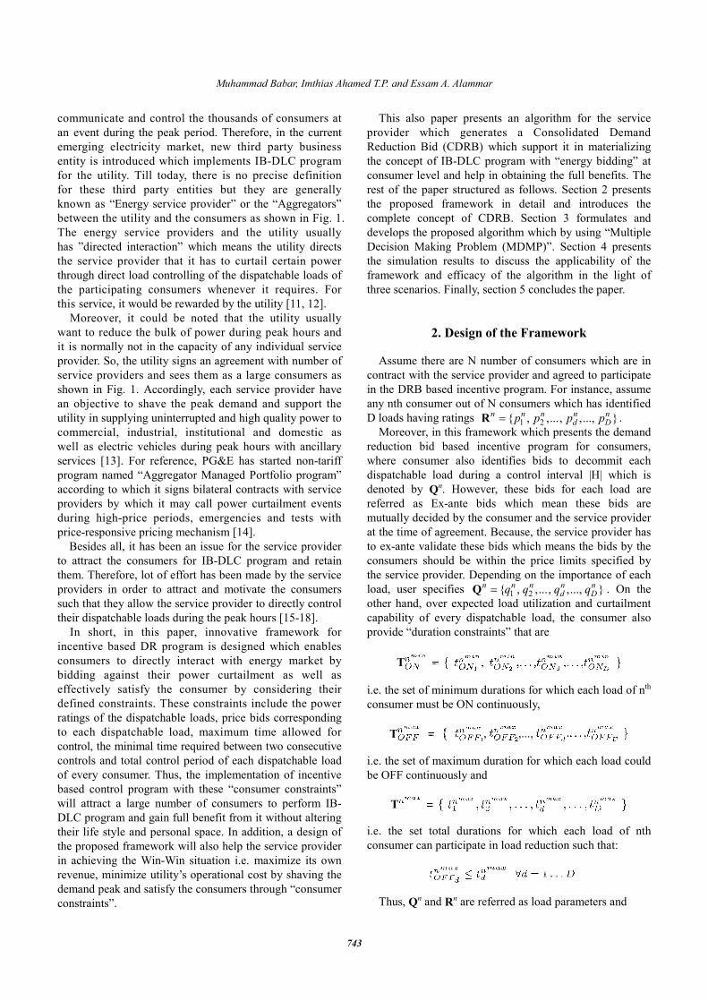
3. Algorithm In this section, the algorithm for the proposed model of

the framework is presented. In order to find out the optimal solution of the discussed control problems, algorithm is divided into five blocks as shown in Fig. 2. Following subsection discusses these blocks in detail.

It can be recalled that the service provider and the

Fig.


746

,...,PiN* (k)) during

. On the other hand, the summation of DRBs corresponding to optimal power

results in consolidated demand ). Hence,

present optimal demand reduction bid (DRB) of each N cumulative power reduction

In summary, CDRB for a given control interval consist of a particular cumulative power reduction level CPi(k) and

which service provider has consumers according to the

corresponding optimal demand reduction bid of each

(4)

In this section, the algorithm for the proposed model of the framework is presented. In order to find out the optimal solution of the discussed control problems, algorithm is

into five blocks as shown in Fig. 2. Following subsection discusses these blocks in detail.

It can be recalled that the service provider and the

consumers has already signed an agreement according to which each consumer has already validated its consumer constraints with the service provider. So, the database of the service provider already has complete information of all N consumers regarding their consumer constraints

Therefore, if the consumer want

any of its consumer constraint then it has to perform it before the control period, or in case he/she changes it in between any control period then it will be effective after that particular control period. Because, before the initialization of the algorithm for the given control period, it is uploaded with the consumer constraints that are in the database at that time. In Fig. 2, intermediate duration variables

, and {a, b, p} corresponds to Moreover, the algorithm divides control period of ‘

hours into control intervals such that each control interval could be of few ‘m’ minutes. Thus, the total number of control intervals ‘K’ for the given control period would be

3.1 Load Monitoring

The algorithm starts from load monitoring block. In this

block, at k = 0 algorithm initially scans all the devices of each consumer by sending monitoring signals. In response, every device of each consumer acknowledge their status through the single boolean variable i.e.‘0’, then it means that the particular consumer is physically OFF or not allowed for control. On other hand, If is ‘1’, then the particular the nth consumer is physically ON and is

2: Block Diagram of the proposed algorithm.


consumers has already signed an agreement according to which each consumer has already validated its consumer constraints with the service provider. So, the database of the service provider already has complete information of

consumers regarding their consumer constraints

Therefore, if the consumer want to make in change in any of its consumer constraint then it has to perform it before the control period, or in case he/she changes it in between any control period then it will be effective after that particular control period. Because, before the initialization of the algorithm for the given control period, it is uploaded with the consumer constraints that are in the database at that time. In Fig. 2, {w, y, z} corresponds to ntermediate duration variables , and

corresponds to {An(k) ,Qn , Rn}. Moreover, the algorithm divides control period of ‘H’

hours into control intervals such that each control interval ’ minutes. Thus, the total number of

’ for the given control period would be

.

The algorithm starts from load monitoring block. In this algorithm initially scans all the devices of

each consumer by sending monitoring signals. In response, every device of each consumer acknowledge their status

the single boolean variable i.e. . If is ‘0’, then it means that the particular dth device of nth

consumer is physically OFF or not allowed for control. On is ‘1’, then the particular dth load of

consumer is physically ON and is available for


control.

3.2 Finding DRB Assume that the availability vector

An(0) = for N consumers. This subsection will first explain how DRB for k=0 is obtained by all N consumers and then how DRB for k=1 to H will be obtained.

As explained earlier, once An(0) is known, algorithm can find various power levels that can be curtailed, e.g.

for all Once the power levels are determined, algorithm can obtain f (Pn(0)) by solving the optimization problem given in Eq. (1) by using dynamic programming (DP) for all consumers as explained in [19].

It can be recalled that the solution of the optimization problem will give

Thus, the algorithm will find and store DRB for all

consumers n=1 ...N. At k =0; then these evaluated DRB

municated to the “Finding CDRB Block” of the algorithm. For k =1...K, this block will always have an updated availability vector An(k), then the DRBconsumers is computed as explained earlier.

3.3 Finding CDRB

Now, DRB Thus, this block will first find the different possible

cumulative power levels that can be curtailed, e.g. CP2(0), ..., CPi(0), ..., CPI(0) for all N consumers. Once the cumulative power levels are determined, then this block can compute F(CPi(0)) by solving the optimization problem given in Eq. (2) by using dynamic programming (DP) for all N consumers as explained in [20].

Similarly, the solution of the problem is stored as

CDRBi(0) = [CPi(0),F(CPi(0)), DRB Then, this set of CDRB is transferred to “Decision

Block”, where the operator of the service provider will take a decision on the basis of the demand identified by the utility. Similarly, for all k =1...K, this block computes the CDRB whenever it is updated with the DRBs from the previous block as shown in Fig. 2.

3.4 Decision Block

If an operator selects the appropriate cumulative power

level CPi∗(0) at k =0. Then in the response, the system will generate direct load control signals for all loads of eaconsumers by using the control string


747

is specified consumers. This subsection will first explain how

consumers and then how

is known, algorithm can find various power levels that can be curtailed, e.g.

for all N consumers. Once the power levels are determined, algorithm can

by solving the optimization problem given using dynamic programming (DP) for all N

It can be recalled that the solution of the optimization

Thus, the algorithm will find and store DRB for all

0; then these evaluated DRB will be com-municated to the “Finding CDRB Block” of the algorithm.

, this block will always have an updated DRB(k) for all N

consumers is computed as explained earlier.

is known. Thus, this block will first find the different possible

cumulative power levels that can be curtailed, e.g. CP1(0), consumers. Once the

cumulative power levels are determined, then this block by solving the optimization

by using dynamic programming consumers as explained in [20].

problem is stored as

DRB∗i(0)]i=1...I

Then, this set of CDRB is transferred to “Decision Block”, where the operator of the service provider will take a decision on the basis of the demand identified by the

, this block computes the ed with the DRBs from the

If an operator selects the appropriate cumulative power . Then in the response, the system will

generate direct load control signals for all loads of each

S It can be recalled that control string present the control

actions i.e. ON or OFF for all Then, the direct load control signals will be communicated to the consumer through two-way communication channel. Based on the communication received, controller in the consumer premises will switch ON or OFF the load. It may be noted that the availability vector the updated consumer constraints and hence CDRB will depend on the service provider choice

On the other hand, if an operator does not want to curtail power from all N consumers, then the operator selects CP1(k) for that particular kth interval. Afterwards, algorithm proceeds as described.

3.5 Updating constraints

For k = 0, variables [

uploaded by algorithm with [0,0,0]. Now,monitoring signals, for k = 0 such that

These uploaded values of constraints and availability

variable is used for evaluating CDRB during interval. Similarly, before evaluating CDRB for all control intervals i.e. k=1...K, the algorithm updates intermediate variables and An(k) over the service provider’s choice

S

Since, this block knows through monitoring block that

which all devices are ON or OFF at that given interval. If the d th of n th consumer device is switched OFF, then for all k=1...K interval these intermediate variables as:

if dth device of nth consumer is switched ON, then for all 1...K interval these intermediate variables are calculated as:

Next step is to find for all

that depends on and . Then,

shown in state transition diagram in Fig. 3. In this state diagram, the transition conditions for the possible

].

It can be recalled that control string present the control actions i.e. ON or OFF for all dth load of the N consumers. Then, the direct load control signals will be communicated

way communication channel. Based on the communication received, controller in the consumer premises will switch ON or OFF the load. It may be noted that the availability vector An(k) as it depends on the updated consumer constraints and hence CDRB will

end on the service provider choice i∗ for k = 1...K. On the other hand, if an operator does not want to curtail

consumers, then the operator selects interval. Afterwards, algorithm

, , ] are uploaded by algorithm with [0,0,0]. Now, Based on the

= 0 algorithm updates the and (k)

These uploaded values of constraints and availability variable is used for evaluating CDRB during k = 0 control interval. Similarly, before evaluating CDRB for all control

, the algorithm updates intermediate the service provider’s choice

.

Since, this block knows through monitoring block that which all devices are ON or OFF at that given interval. If

consumer device is switched OFF, then for all interval these intermediate variables are calculated

consumer is switched ON, then for all k =

interval these intermediate variables are calculated as:

for all d . It may be recalled and as well as

. Then, is calculated as shown in state transition diagram in Fig. 3. In this state diagram, the transition conditions for the possible


transitions are:

To understand the functionality and transition of

availability variable and(k) from (k−1) control interval to

kth interval, consider the same nth consumer as shown in Table 1 having the availability vector{which is a set of availability variables for the stated six devices. Then, and means 1st, 2nd and 3rd dispatchable load is ON and can be switched OFF. = 0; means the 4th load was switched OFF during the previous interval i.e. (k remain switched OFF or turn ON during this the condition that denotes the duration for which the 4th load is continuously

OFF during kth interval. Suppose, at (k−1)th interval, 4th was switched OFF and at tn

OFF4(k) = 10 min. Then, at kth interval there could be two possible values of i.e “0” - it remains switched OFF even during kth interval otherwise means 5th load is ON and it can not be switched OFF until

where denotes the duration for which the 5th load is continuously ON during

= z; means 6th load is not in control mode i.e. it is either physically switched OFF by the consumer or it is not participating at all during the control period due to anyreason.

Thus, it can be observed the availability of a device depends not only on ,

maxntalso depends on the duration for which the particular device was continuously ON or OFF before the current interval. These intermediate variables are denoted by [ , , ] and will be explain in detail in the next section.

Once the An(k) is updated for the preceding interval, then algorithm on the basis this monitoring signal, for 1...K algorithm updates the such that

Fig. 3: Transition diagram of availability variable


748

To understand the functionality and transition of control interval to

consumer as shown in 1 having the availability vector An(k) =

{ x,x,x,0,1,z } is a set of availability variables for the stated six

is equal to “x”; dispatchable load is ON and can be

load was switched k − 1) and might

remain switched OFF or turn ON during this kth interval on where

load is continuously = 20 min. Let

was switched OFF and at kth interval interval there could be two

it remains switched OFF = 1;

load is ON and it can not be switched OFF untildenotes the duration for

load is continuously ON during kth interval. load is not in control mode i.e. it is

either physically switched OFF by the consumer or it is not participating at all during the control period due to any

Thus, it can be observed the availability of a device and ,

maxnt but it also depends on the duration for which the particular device was continuously ON or OFF before the current interval. These intermediate variables are denoted by

and will be explain in detail in

is updated for the preceding interval, then algorithm on the basis this monitoring signal, for k =

such that

Thus, this time rest of the blocks of the algorithm uses intermediate duration variables and updated availability vector for the evaluation of CDRB.

4. Case Study The aim of this case study is to discuss the efficacy of

the proposed algorithm for the presented model of the framework. The proposed algorithm is investigated by considering five different domestic consumers. It is assumed that these consumers hacontract with the service provider. It can be recalled that at the time of agreement, consumers identify their consumer constraints for all of their dispatchable load as illustrated in Table 2.

It is assumed that the energy servidirect load control program to the continuously running thermal loads. In DLC, the most significant and focused dispatchable loads for control are Electric Heaters or Air conditioners because they are usually the highest energy consuming domestic loads. However, many medium energy consuming loads like refrigerators are also considers as a targeted dispatchable loads in this case study.

Generally, the power ratings of the domestic Electric Heater or Air-conditioners are around 750W upto 2.5kW and the power rating of refrigerators are around 350W to 800W depending on the capacity of the appliance. So, it can be observed that different powefor the devices of each consumers in order to check the effectiveness of algorithm. Moreover, it can be recalled that

: Transition diagram of availability variable .

Table 2. Consumer constraints of five


,maxnt

Thus, this time rest of the blocks of the algorithm uses intermediate duration variables and updated availability vector for the evaluation of CDRB.

e Study

The aim of this case study is to discuss the efficacy of the proposed algorithm for the presented model of the framework. The proposed algorithm is investigated by considering five different domestic consumers. It is assumed that these consumers have signed up the bilateral contract with the service provider. It can be recalled that at the time of agreement, consumers identify their consumer constraints for all of their dispatchable load as illustrated in

It is assumed that the energy service provider deploy direct load control program to the continuously running thermal loads. In DLC, the most significant and focused dispatchable loads for control are Electric Heaters or Air conditioners because they are usually the highest energy

domestic loads. However, many medium energy consuming loads like refrigerators are also considers as a targeted dispatchable loads in this case study.

Generally, the power ratings of the domestic Electric conditioners are around 750W upto 2.5kW

and the power rating of refrigerators are around 350W to 800W depending on the capacity of the appliance. So, it can be observed that different power ratings are considered for the devices of each consumers in order to check the effectiveness of algorithm. Moreover, it can be recalled that

constraints of five consumers


bidding to the each load by the consumers will identify the “Desire of Use” of the consumers. So, here, in the Tait can be seen that consumer 5 assigns 0.54units/hr to its load while on the same side it assigns 1.8units/hr to its load. It means that 2nd load has more significance than the 4th load for the 5th consumer.

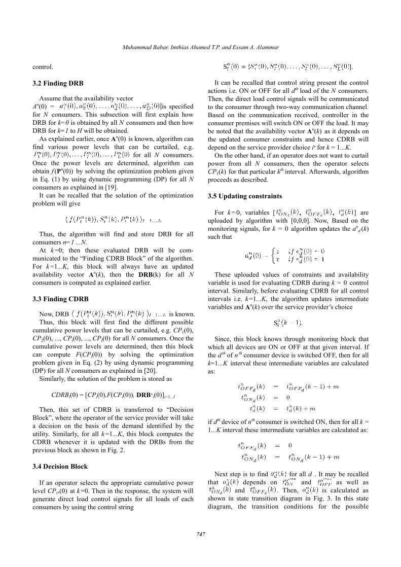
It can also be recalled that the utility and the service provider has directed interaction as per their agreement. According to this, the utility has to provide an expected demand curve respective five consumers to the service provider, as shown in Fig. 4. In this Fig. 4, the utility wantsthat the service provider should control the loads from 9:00AM till 9:00PM i.e. the control period of 12 hrs. Moreover, it can be recalled that by the proposed framework, the utilities should also indicate the baseof the bulk of the power that the service providers has to maintain through load management and result in shaving the demand curve during the peak hours. In this case study, it is assumed that utility identifies the service provider to shave the demand curve at 18.5kW. On the other hand, thservice provider is also paid for it DLC services by the utility. Here, it is assumed that the utility will pay a fixed reward of 5 units/hour to the service provider.

Now, for the purpose of simulations, it is assumed that control period of 12hours is divided in to K=72 control

Fig. 4. Demand curve supplied by the utility to the service provider.

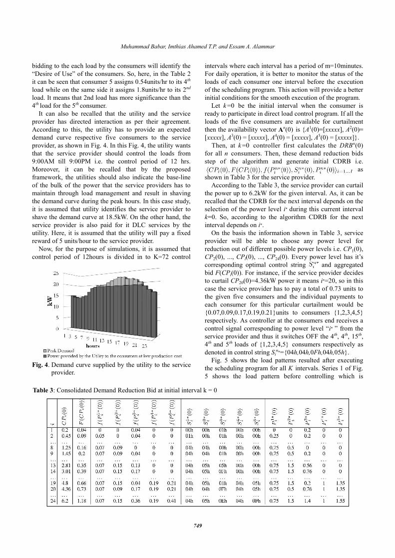
Table 3: Consolidated Demand Reduction Bid at initial interval


749

bidding to the each load by the consumers will identify the “Desire of Use” of the consumers. So, here, in the Table 2 it can be seen that consumer 5 assigns 0.54units/hr to its 4th

load while on the same side it assigns 1.8units/hr to its 2nd

load. It means that 2nd load has more significance than the

tility and the service provider has directed interaction as per their agreement. According to this, the utility has to provide an expected demand curve respective five consumers to the service provider, as shown in Fig. 4. In this Fig. 4, the utility wants that the service provider should control the loads from 9:00AM till 9:00PM i.e. the control period of 12 hrs. Moreover, it can be recalled that by the proposed framework, the utilities should also indicate the base-line

ervice providers has to maintain through load management and result in shaving the demand curve during the peak hours. In this case study, it is assumed that utility identifies the service provider to shave the demand curve at 18.5kW. On the other hand, the service provider is also paid for it DLC services by the utility. Here, it is assumed that the utility will pay a fixed reward of 5 units/hour to the service provider.

purpose of simulations, it is assumed that control period of 12hours is divided in to K=72 control

intervals where each interval has a period of m=10minutes. For daily operation, it is better to monitor the status of the loads of each consumer one intervaof the scheduling program. This action will provide a better initial conditions for the smooth execution of the program.

Let k =0 be the initial interval when the consumer is ready to participate in direct load control program. If all the loads of the five consumers are available for curtailment then the availability vector An(0) [xxxxx], A3(0) = [xxxxx], A4(0) = [

Then, at k =0 controller first calculates the for all n consumers. Then, these demand reduction bids step of the algorithm and generate initial CDRB i.e.

shown in Table 3 for the service provider.According to the Table 3, the

the power up to 6.2kW for the given interval. As, it can be recalled that the CDRB for the next interval depends on the selection of the power level i∗k=0. So, according to the algorithm CDRB fointerval depends on i∗.

On the basis the information shown in Table 3, service provider will be able to choose any power level for reduction out of different possible power levels i.e. CP2(0), ..., CPl(0), ..., CP24(0)corresponding optimal control string bid F(CPi(0)). For instance, if the service provider decides to curtail CP20(0)=4.36kW power it means case the service provider has to pay a total of 0.73 the given five consumers and the individual payments to each consumer for this particular curtailment would be {0.07,0.09,0.17,0.19,0.21}units to consumers respectively. As controller at the consumers end receives a control signal corresponding to power level “service provider and thus it switches OFF the 4th and 5th loads of {1,2,3,4,5denoted in control string Si

n∗={04Fig. 5 shows the load patterns resulted after executing

the scheduling program for all 5 shows the load pattern before controlling which is

urve supplied by the utility to the service

: Consolidated Demand Reduction Bid at initial interval k = 0

intervals where each interval has a period of m=10minutes. For daily operation, it is better to monitor the status of the loads of each consumer one interval before the execution of the scheduling program. This action will provide a better initial conditions for the smooth execution of the program.

the initial interval when the consumer is ready to participate in direct load control program. If all the loads of the five consumers are available for curtailment

(0) is {A1(0)=[xxxxx], A2(0)= 0) = [xxxxx], A5(0) = [xxxxx]}.

controller first calculates the DRBn(0) consumers. Then, these demand reduction bids the algorithm and generate initial CDRB i.e.

as shown in Table 3 for the service provider.

According to the Table 3, the service provider can curtail the power up to 6.2kW for the given interval. As, it can be recalled that the CDRB for the next interval depends on the ∗ during this current interval

. So, according to the algorithm CDRB for the next

On the basis the information shown in Table 3, service provider will be able to choose any power level for reduction out of different possible power levels i.e. CP1(0),

(0). Every power level has it’s corresponding optimal control string and aggregated

. For instance, if the service provider decides =4.36kW power it means i∗=20, so in this

case the service provider has to pay a total of 0.73 units to the given five consumers and the individual payments to each consumer for this particular curtailment would be

units to consumers {1,2,3,4,5} respectively. As controller at the consumers end receives a

esponding to power level “i∗ ” from the service provider and thus it switches OFF the 4th, 4th, 15th,

} consumers respectively as {04h,04h,0Fh,04h,05h}.

Fig. 5 shows the load patterns resulted after executing the scheduling program for all K intervals. Series 1 of Fig. 5 shows the load pattern before controlling which is


750

composed of both the controllable and uncontrollable loads. Series 2 of Fig. 5 shows the load pattern of ideal controlling in which program is executed with a fixed targeted level of 18.5kW and Fig. 6 shows the power reduced by each consumer as well as their aggregated reduction during each control interval.

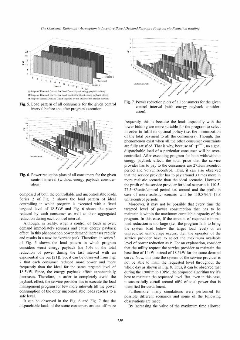
Although, in reality, when a control of loads is over, demand immediately resumes and cause energy payback effect. In this phenomenon power demand increases rapidly and results in a new inadvertent peak. Therefore, in series 3 of Fig. 5 shows the load pattern in which program considers worst energy payback (i.e 50% of the total reduction of power during the last interval with an exponential die out [21]). So, it can be observed from Fig. 7 that each consumer reduced more power and more frequently than the ideal for the same targeted level of 18.5kW. Since, the energy payback effect exponentially decreases. Therefore, in order to completely avoid the payback effect, the service provider has to execute the load management program for few more intervals till the power consumption of the other uncontrollable loads reaches to a safe level.

It can be observed in the Fig. 6 and Fig. 7 that the dispatchable loads of the some consumers are cut off more

frequently, this is because the loads especially with the lower bidding are more suitable for the program to select in order to fulfil its optimal policy (i.e. the minimization of the total payment to all the consumers). Though, this phenomenon exist when all the other consumer constraints are fully satisfied. That is why, because of maxnT , no signal dispatchable load of a particular consumer will be over-controlled. After executing program for both with/without energy payback effect, the total price that the service provider has to pay to the consumers are 27.5units/control period and 96.7units/control. Thus, it can also observed that the service provider has to pay around 3 times more in more realistic scenario than the ideal scenario. However, the profit of the service provider for ideal scenario is 110.5-27.5=83units/control period i.e. around and the profit in case of more-realistic scenario will be 110.5-96.7=13.8 units/control periods.

Moreover, it may not be possible that every time the targeted level of power consumption that has to be maintain is within the maximum curtailable capacity of the program. In this case, If the amount of required minimal load reduction is too large (i.e., the program fails to bring the system load below the target load level) or an unpredicted unit outage occurs, then the operator of the service provider have to select the maximum available level of power reduction as i∗. For an explanation, consider that the utility request the service provider to maintain the base-line of 14kW instead of 18.5kW for the same demand curve. Now, this time the system of the service provider is not be able to main the requested level throughout the whole day as shown in Fig. 8. Thus, it can be observed that during the 1:00Pm to 10PM, the proposed algorithm try it’s best to maintain the requested level. But, even in this case, it successfully curtail around 60% of total power that is identified for curtailment.

Furthermore, many simulations were performed for possible different scenarios and some of the following observations are made:

By increasing the value of the maximum time allowed

Fig. 5. Load pattern of all consumers for the given control

interval before and after program execution.

Fig. 6. Power reduction plots of all consumers for the given

control interval (without energy payback consider-ation).

Fig. 7. Power reduction plots of all consumers for the given

control interval (with energy payback consider-ation).


751

for control maxnOFFT and decreasing the minimal time

required between control intervals mixnONT , the service

provider could increase its capability of power reduction but it will effect both the consumer “Desire of Use” and energy payback.

If the power to be curtailed during the interval is around one-third of the maximum capacity of the service provider. Then the service provider will never face a problem of incapability of power reduction.

5. Conclusion In conclusion, the proposed framework of an aggregated

demand response program for the constrained direct load control in order to achieve the grid stability and operational cost minimization during the peak demand is mathemati-cally formulated. The framework by introducing the concept of demand reduction bidding and duration constraints in direct load control attempts to benefit and satisfy all the stakeholders i.e. the utility, the aggregator and the consumers.

The proposed algorithm for the framework computes the consolidated demand reduction bidding while considering all consumers’ load parameters and constraints. This in exchange gives optimal load scheduling to the aggregator. The simulation results of the case studies exemplify the proof-of-concept of the algorithm and the mathematical framework. Moreover, demand reduction bidding in constrained direct load control could achieve more consumer penetration and better load management than the conventional. Thus, it could also be evaluated that by this approach the aggregators could act more effectively in the smart grid paradigm.

References

[1] S. Amin, “For the good of the grid,” IEEE Power and Energy Magazine, vol. 6, no. 6, pp. 48-59, 2008.

[2] “Us department of energy - smart grid.” [Online]. Available: http://energy.gov/oe/technologydevelopment/smart-grid

[3] B. Kirby, Spinning reserve from responsive loads. Department of Energy-United States. 2003.

[4] M. Albadi and E. El-Saadany, “A summary of demand response in electricity markets,” Electric Power Systems Research, vol. 78, no. 11, pp. 1989-1996, 2008.

[5] J. Torriti, M. G. Hassan, and M. Leach, “Demand response experience in europe: Policies, programmes and implementation,” Energy, vol. 35, no. 4, pp. 1575-1583, 2010.

[6] D. S. Kirschen, “Demand-side view of electricity markets,” Power Systems, IEEE Transactions on, vol. 18, no. 2, pp. 520-527, 2003.

[7] B. F. Hobbs, H. Rouse, and D. T. Hoog, “Measuring the economic value of demand-side and supply re-sources in integrated resource planning models,” Power Systems, IEEE Transactions on, vol. 8, no. 3, pp. 979-987, 1993.

[8] A. Brooks, E. Lu, D. Reicher, C. Spirakis, and B. Weihl, “Demand dispatch,” IEEE Power and Energy Magazine,, vol. 8, no. 3, pp. 20-29, 2010.

[9] M. Babar, T.A. Taj, T.I. Ahamed, and E.A. AlAmmar, “The conception of the aggregator in demand side management for domestic consumers,” 2013.

[10] M. Babar, T.A. Taj, T.I. Ahamed, and I. Ijaz, “Design of a framework for the aggregator using demand reduction bid (drb),” Journal of Energy Technologies and Policy, vol. 4, no. 1, pp. 1-7, 2014.

[11] P. Samadi, H. Mohsenian-Rad, R. Schober, and V. Wong, “Advanced demand side management for the future smart grid using mechanism design,” IEEE Transactions on Smart Grid, vol. 3, no. 3, pp. 1170- 1180, 2012.

[12] R. Yu, W. Yang, and S. Rahardja, “Optimal real-time price based on a statistical demand elasticity model of electricity,” in First International Workshop on Smart Grid Modeling and Simulation (SGMS), 2011 IEEE. IEEE, 2011, pp. 90-95.

[13] C. Puckette, G. Saulnier, R. Korkosz, and J. Hershey, “Ghm aggregator,” Feb. 12 2002, uS Patent

[14] 6,346,875. [15] “Aggregator managed portfolio (amp) program,

pacific gas and electric company.” [Online]. Avail-able: http://www.pge.com/mybusiness /energysaving srebates/demandresponse/amp/

[16] H. Salehfar, P. Noll, B. LaMeres, M. Nehrir, and V. Gerez, “Fuzzy logic-based direct load control of residential electric water heaters and air conditioners recognizing customer preferences in a deregulated environment,” in IEEE Power Engineering Society Summer Meeting, 1999., vol. 2. IEEE, 1999, pp. 1055-1060.

Fig. 8. Aggregated load pattern of all n consumers when

the utility request base-line of 14kW.


752

[17] H. Jorge, C. Antunes, and A. Martins, “A multiple objective decision support model for the selection of remote load control strategies,” IEEE Transactions on Power Systems, vol. 15, no. 2, pp. 865-872, 2000.

[18] K. Huang and Y. Huang, “Integrating direct load control with interruptible load management to pro-vide instantaneous reserves for ancillary services,” IEEE Transactions on Power Systems, vol. 19, no. 3, pp. 1626-1634, 2004.

[19] I. Cobelo, “Active control of distribution networks,” Ph.D. dissertation, The University of Manchester, 2005.

[20] M. Babar, I. Ahmed, A. Shah, S. Al Ghannam, E. AlAmmar, N. Malik, and F. Pazehri, “An algorithm for load curtailment in aggregated demand response program,” in 2012 IEEE PES Conference on Inno-vative Smart Grid Technologies-Middle East (ISGT Middle East). IEEE, 2012.

[21] M. Babar, T. Imthias Ahamed, E. A. Al-Ammar, and [22] A. Shah, “A novel algorithm for demand reduction [23] bid based incentive program in direct load control,”

Energy Procedia, vol. 42, pp. 607-613, 2013. [24] T. Ericson, “Direct load control of residential water

heaters,” Energy Policy, vol. 37, no. 9, pp. 3502- 3512, 2009.

Muhammad Babar received his BE in Electronic Engineering by the NEDUET in 2010, and MS in Manufacturing System Design and Management Engineering by the NUST, Pakistan in 2013Currently, he is working as a PhD student at the Electrical Power Systems (EES) Group,

Technology University of Eindhoven, Netherlands. His research is focused on services that enhance the demand response capability of distribution networks.

Imthias Ahamed received his B.Tech degree in electrical engineering from Kerala University and M. Tech degree in instrumentation and control from NIT-Calicut, India. He obtained his Ph.D from Indian Institute of Science, Bangalore, India in 2002. He is now an assistant professor with Department of

Electrical and Computer Engineering, College of Engi-neering, Dhofar University, Salalah, Sultanate of Oman. His current research include reinforcement learning, demand response, distributed generation, neural networks and power system scheduling and control.

Essam Abdulaziz Al-Ammar is an Associate Professor in the Department of Electrical Engineering at King Saud University in Riyadh, Saudi Arabia. Previously, Prof. Al-Ammar was an advisor at the Ministry of Water and Electricity (MOWE) and an Energy Consultant for Riyadh Techno Valley

(RTV). He also worked as a Power/Software Engineer at Lucent Technologies in Riyadh for two years. He is a member of various local and international committees concerned with different aspects of power and electrical energy. His current interests include high voltage engi-neering, power system transmission and distribution, as well as renewable energy and smart grids. Prof. Al-Ammar received his MS degree from the University of Alabama in 2003, and earned a PhD from Arizona State University in 2007. He has been a Senior member of the Institute of Electrical and Electronics Engineers (IEEE) since 2007, and has sat on the Saudi Engineering Committee since 1997.

The Consumer Rationality Assumption in Incentive Based Demand Response Program via Reduction Bidding

Documents

Transcript of The Consumer Rationality Assumption in Incentive Based Demand Response Program via Reduction Bidding