Market equilibria under procedural rationality

Market Equilibria under Procedural Rationality∗

Mikhail Anufriev a,b,† Giulio Bottazzi b,‡

a CeNDEF, Department of Economics, University of Amsterdam,

Roetersstraat 11, NL-1018 WB Amsterdam, Netherlands

b LEM, Scuola Superiore Sant’Anna,

Piazza Martiri della Liberta 33, 56127 Pisa, Italy

∗We thank Pietro Dindo, Cars Hommes, Marco Lippi, Francesca Pancotto, Angelo Secchi, the participants

of the seminars, conferences and workshops in Amsterdam, Bielefeld, Kiel, Pisa and Washington, and especially

an anonymous referee for useful discussions and helpful comments and suggestions. This work was supported

by the ComplexMarkets E.U. STREP project 516446 under FP6-2003-NEST-PATH-1.†Tel.: +31-20-5254248; fax: +31-20-5254349; e-mail: [email protected].‡Corresponding author. Tel.: +39-050-883365; fax: +39-050-883344; e-mail: [email protected].

1

Abstract

We analyze the endogenous price formation mechanism of a pure exchange economy

with two assets, riskless and risky. The economy is populated by an arbitrarily large

number of traders whose investment choices are described by means of generic smooth

functions of past realizations. These choices can be consistent with (but not limited to)

the solutions of expected utility maximization problems.

Under the assumption that individual demand for the risky asset is expressed as a

fraction of individual wealth, we derive a complete characterization of equilibria. It is

shown that irrespectively of the number of agents and of their behavior, all possible

equilibria belong to a one-dimensional “Equilibrium Market Curve”. This geometric

tool helps to illustrate the possibility of different phenomena, as multiple equilibria, and

can be used for comparative static analysis. We discuss the relative performances of

different strategies and the selection principle governing market dynamics on the basis

of the stability analysis of equilibria.

JEL codes: G12, D83.

Keywords: Asset Pricing Model, Procedural Rationality, Heterogeneous Agents, CRRA

Framework, Equilibrium Market Curve, Stability Analysis, Multiple Equilibria.

2

1 Introduction

There exists a long-standing tradition in theoretical economics to model economic agents as

having a strictly limited range of notionally available actions. Maximization of a suitable

function (e.g. expected utility) is widely accepted as a reasonable description of individual

behavior, as it captures the idea of rationality and profit seeking behind the actions of the

“economic man”. As early as fifty years ago, however, some writers, most notably Herbert

Simon, recognized a strong dissonance between the modeling of human behavior in economics

and the description of the same behavior in other social sciences. Indeed Simon (1955) em-

phasizes that, due to informational and cognitive restrictions, people may not be acting as if

they were utility maximizers who are able to perfectly anticipate their own and others’ future

decisions and reactions. At the same time, however, it is in general true that human beings

avoid behaving in a random manner. Rather they tend to follow some deliberate procedures in

their decision making process. This broader view on economic behavior led to the concept of

procedural rationality (Simon, 1976) which still includes, as a special case, the optimizing and

perfectly anticipating behavior but which can, at the same time, account for different types

of learning.

The assumption of procedurally rational agents implies that the level of heterogeneity in

the market is much larger than it is usually assumed. As argued by Kirman (2006) this

heterogeneity is probably fundamental for the functioning of market economies. Notice that,

in principle, even “substantive rational” agents imbued with perfectly anticipating rationality

may differ in terms of their preference structure and, hence, in their implied actions. At the

same time, heterogeneity in expectations is reported in several surveys on traders behavior

and is the basis for several proposed explanations for the abnormal large trading volume in

financial markets and for other observed “anomalies” (e.g. Brock (1997); Hommes (2006) and

references therein). Such “rational heterogeneity” is broaden and strengthen by the various

violations of axioms of rational choice which have been well documented by a number of

different studies in the field of experimental economics1.

1The Handbook of Experimental Economics (Kagel and Roth, 1995) and the Nobel lecture of Daniel

3

If the evidence supports the idea of procedural rationality of heterogeneous agents, why

do the models based on that assumption remain exceptions rather than norm? In his review

of the literature on bounded rationality, Conlisk (1996) identifies a number of possible reasons

for the dominance of substantive rational behavior in economic modeling. One of them is that

such behavior, even if not entirely realistic, seriously restricts the range of possible actions,

and, hence, brings discipline into the theory. By acknowledging the need of discipline, this

paper seeks to dispel the fear of getting lost in the “wilderness of bounded rationality”. In the

context of a simple speculative asset market our model demonstrates that (i) market forces

and (ii) a natural requirement for consistency between aggregate dynamics and individual

actions will lead to quite specific conclusions about the long-run state of the market.

We consider a dynamic model where an arbitrary number of heterogeneous agents trade

a riskless bond and a long-lived risky asset. The only restriction imposed on the individual

behavior is that the amount of asset demanded by traders is expressed as a fraction of their

current wealth. In technical terms, this assumption confines possible agents’ behavior to the

so-called constant relative risk aversion (CRRA) framework. The shares of personal wealth

invested in the risky security are chosen, at each period, following individual procedures and

on the basis of commonly available information. We model procedural rationality by means of

agent-specific investment functions which map the information set to the present investment

share. The dynamics of the multi-dimensional system describing the evolution of asset price

and agents’ wealth is derived. Without imposing any constraint about the specific form of the

investment functions we are able to completely characterize those equilibria in which aggregate

market dynamics is consistent with agents expectations. Equilibrium price return and wealth

distribution turn out to be a combined outcome of the agents’ adaptive procedures and of

the evolutionary selection taking place in the market. Specifically, we show that two types

of long-run dynamics are possible. In the first type both securities give the same expected

return, and the wealth of all agents grows at the same rate. In the second type one of the

Kahneman (Kahneman, 2003) provides plenty of examples of systematic biases, i.e. individual decisions which

would be qualified as irrational from the traditional economic point of view.

4

securities gives a higher expected return, and one or few “survivors” ultimately possess the

total wealth of the economy. We derive the local stability results for all possible steady-states.

The conditions are ready to be applied for any specific ecology of traders whose behavior can

be accommodated in our framework.

Two distinct streams of theoretical research intersect in our paper. The main source of

our inspiration is the growing field of the Heterogeneous Agent Models (HAMs), extensively

reviewed in Hommes (2006). The HAM literature considers markets as a feedback system,

where agents employ adaptive expectation rules, so that current prices affect expectations

about future prices, and, consequently, prices themselves. Modeling stylized behaviors of

“fundamentalists” or “trend chasers”, the HAMs can explain different “stylized facts” of fi-

nancial markets, such as excess volatility and repeated patterns of temporary bubbles followed

by severe crashes. In our opinion, however, this approach lacks an unifying framework, be-

cause expectation rules vary from model to model. By keeping investment functions generic we

intend to create such a framework, avoiding, at the same time, an unrealistic level of simplic-

ity in the agents’ expectational procedures and considering truly heterogeneous preferences.

Furthermore, in the HAMs with evolving population (as e.g. in Brock and Hommes (1998)),

agents switch between different forecasting rules on the basis of some performance measure,

which is often introduced ad hoc. Conversely, the wealth dynamics, explicitly considered in

our framework, provide a natural performance measure.2

Multi-asset markets populated by several procedurally rational agents are studied in the

literature on Evolutionary Finance (EF), initiated by Blume and Easley (1992), and recently

2Our paper can be considered as only a first step towards an unifying framework of the HAM literature.

An issue is that many HAMs are built in the so-called constant absolute risk aversion (CARA) framework,

which is outside of the scope of this paper. In the CARA framework agents’ demand is independent of their

wealth, and thus wealth dynamics do not affect asset pricing. Our framework is, instead, of constant relative

risk aversion (CRRA), where the agents’ investment shares do not depend on their wealth, so that demand for

the risky asset increases linearly with wealth. The inclusion of CARA strategies in a CRRA-based framework

is a subject of future research. Notice, however, that experiments with human subjects usually reject CARA

behavior, supporting decreasing or constant relative risk aversion, see for example Kroll, Levy, and Rapoport

(1988) and the discussion of this issue in Levy, Levy, and Solomon (2000).

5

reviewed in Evstigneev, Hens, and Schenk-Hoppe (2009). Our paper shares a number of dis-

tinctive features with the EF literature, such as a descriptive approach to the investment

behavior of agents and the central role played by the wealth-driven selection in determining

the long-run dynamics of the market. The EF literature focuses on the relative valuation of

different risky assets. It is also specifically interested in a search for those strategies which

attract most wealth and are evolutionary stable, i.e., are not driven out by alternative behav-

iors. In contrast to the EF literature, but in the spirit of the HAMs, in this paper we focus on

the nature of market instabilities caused by the adaptive behavior of agents and the feedback

mechanism existing between realized and expected market conditions. This difference in focus

is reflected in our investment functions, which explicitly depend on past realized returns3

These distinct streams of economic research, the EF and HAMs, meet in the main result of

this paper, the local stability conditions of procedurally consistent equilibria in which aggregate

market dynamics is consistent with agents expectations. We find that two conditions are

necessary and sufficient for the stability of one or many-survivors equilibria. The first is

essentially the requirement of evolutionary stability of the surviving strategies, which is similar

to the “survival” criteria adopted in EF models. The second is the dynamic stability of these

strategies under the price feedback mechanism, a typical result of the HAMs.

The rest of the paper is organized as follows. In Section 2 we introduce the model, pre-

senting and briefly discussing our assumptions. First, we explicitly write the traders’ inter-

temporal budget constraints. Second, we derive the resulting dynamics in terms of returns and

wealth shares. Third, we introduce agent specific investment functions. Finally, we introduce

the notion of Procedurally Consistent Equilibrium that will be used as a formal definition

3There are other details which distinguish our approach from the EF literature. Namely: a risk-free asset

is available in our economy at a given price, we have only one risky asset and we do not let agents consume

all the dividend payoffs. In addition, the earlier EF papers by Hens and Schenk-Hoppe (2005) and Amir,

Evstigneev, Hens, and Schenk-Hoppe (2005) model assets as short-lived and, consequently, ignore capital

gain as a component of agents’ wealth accumulation. The last models of the EF literature (see, e.g., Amir,

Evstigneev, and Xu (2008), Evstigneev, Hens, and Schenk-Hoppe (2006, 2008)) all deal with long-lived assets,

as we do in our framework.

6

of equilibrium throughout the paper. In Section 3 we present the equilibrium and stability

analysis of the system in the simplest case of a single active trader. The geometric locus

of all possible equilibria, the Equilibrium Market Curve, is derived, and its use is discussed.

Then we derive general stability conditions and we discuss few important special cases which

received particular attention from the past literature. Section 4 is devoted to the analysis of

the general case in which an arbitrarily large number of traders are present in the market.

The implications of our findings concerning the general ability of market forces in selecting

the “best” strategy are discussed in Section 4.4 while Section 5 concludes.

2 Model Definition

Consider a simple pure exchange economy where trading activities take place in discrete time.

The economy is composed by a riskless asset (bond) giving in each period a constant interest

rate rf > 0 and a risky asset (equity) paying a random dividend Dt at the beginning of each

period t. The riskless asset is considered the numeraire of economy and its price is fixed to 1.

The ex-dividend price Pt of the risky asset is determined at each period, on the basis of the

aggregate demand, through market-clearing condition. The resulting intertemporal budget

constraint is derived below and the main hypotheses, on the nature of the investment choices

and of the fundamental process, are discussed. These hypotheses will allow us to derive the

explicit dynamical system governing the evolution of the economy.

2.1 Intertemporal budget constraint

We consider general situation when the economy is populated by a fixed number N of traders4.

Let Wt,n and xt,n stand for the wealth of trader n at time t and for the fraction of his

wealth invested into the risky asset. Following Epstein and Zin (1989) and similarly to Amir,

4Using the terminology of the heterogeneous agent literature, we consider N types of traders (cf. Brock,

Hommes, and Wagener (2005)). Notice, however, that all traders possessing the same investment behavior

(type) are considered as one single investor. That is, in the terminology of the evolutionary finance literature

we deal with N different strategies (cf. Hens and Schenk-Hoppe (2005))

7

Evstigneev, Hens, and Schenk-Hoppe (2005) we assume that total agent’s wealth is rein-

vested and ignore consumption. Thus, after the trading session at time t, agent n possesses

xt,n Wt,n/Pt shares of the risky asset and (1− xt,n) Wt,n shares of the riskless security. In the

beginning of time t + 1 the agent gets (in terms of the numeraire) random dividends Dt+1 per

each share of the risky asset and constant interest rate rf for all shares of the riskless asset.

Therefore, at time t + 1 the wealth of agent n is given by

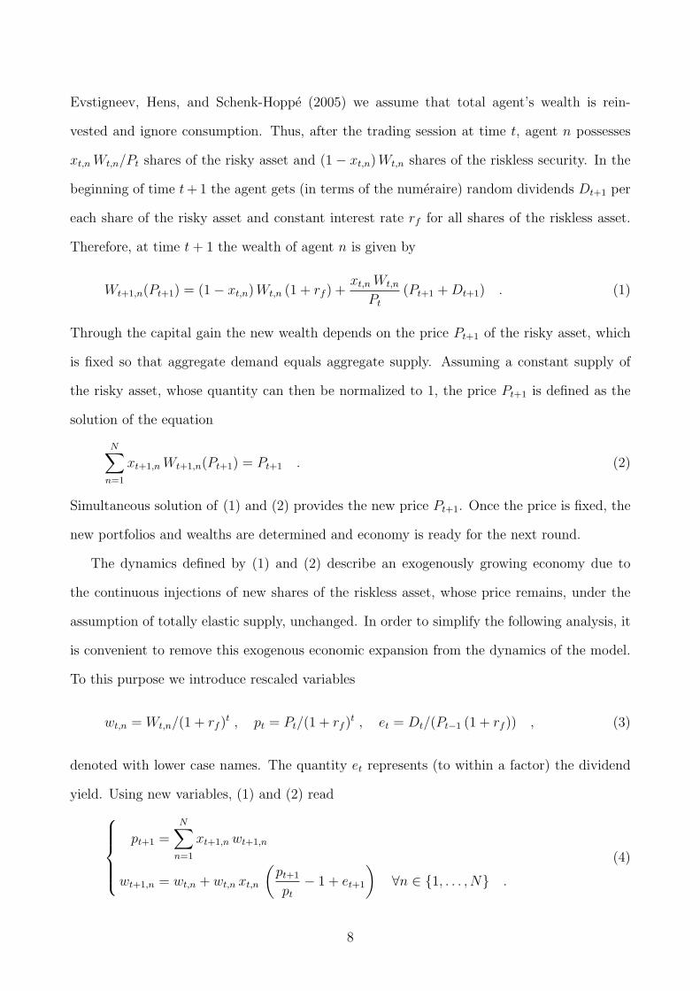
Wt+1,n(Pt+1) = (1− xt,n) Wt,n (1 + rf ) +xt,n Wt,n

Pt

(Pt+1 + Dt+1) . (1)

Through the capital gain the new wealth depends on the price Pt+1 of the risky asset, which

is fixed so that aggregate demand equals aggregate supply. Assuming a constant supply of

the risky asset, whose quantity can then be normalized to 1, the price Pt+1 is defined as the

solution of the equation

N∑n=1

xt+1,n Wt+1,n(Pt+1) = Pt+1 . (2)

Simultaneous solution of (1) and (2) provides the new price Pt+1. Once the price is fixed, the

new portfolios and wealths are determined and economy is ready for the next round.

The dynamics defined by (1) and (2) describe an exogenously growing economy due to

the continuous injections of new shares of the riskless asset, whose price remains, under the

assumption of totally elastic supply, unchanged. In order to simplify the following analysis, it

is convenient to remove this exogenous economic expansion from the dynamics of the model.

To this purpose we introduce rescaled variables

wt,n = Wt,n/(1 + rf )t , pt = Pt/(1 + rf )

t , et = Dt/(Pt−1 (1 + rf )) , (3)

denoted with lower case names. The quantity et represents (to within a factor) the dividend

yield. Using new variables, (1) and (2) read

pt+1 =N∑

n=1

xt+1,n wt+1,n

wt+1,n = wt,n + wt,n xt,n

(pt+1

pt

− 1 + et+1

)∀n ∈ {1, . . . , N} .

(4)

8

These equations represent an evolution of state variables wt,n and pt over time, provided that

stochastic process {et} is given and the set of investment shares {xt,n} is specified.5

In this paper the agents’ investment shares are assumed to be independent of the contempo-

raneous price and wealth, the assumption which will be formalized in Section 2.3. System (4)

implies a simultaneous determination of the equilibrium price pt+1 and of the agents’ wealths

wt+1,n, so that the state of the system at time t + 1 is only implicitly defined. For analytical

purposes, one has to derive the explicit equations that govern the system dynamics.

2.2 The dynamical system for wealth shares and price return

Let an be an agent specific variable, dependent or independent from time t. We denote with⟨a⟩

tits wealth weighted average on the population of agents at time t, i.e.

⟨a⟩

t=

N∑n=1

an ϕt,n , where ϕt,n =wt,n

wt

and wt =N∑

n=1

wt,n. (5)

The transformation of the implicit dynamics (4) into an explicit one is not, in general, possible

also because the market price should remain positive over time. On the other hand, the agents

are allowed to have negative wealth, which is interpreted as debt in that case. Therefore, ϕt,n

are arbitrary numbers whose sum over all agents is equal to 1 for any period t.

The next result gives the condition for which the dynamical system implicitly defined in

(4) can be made explicit without violating the requirement of positiveness of prices.

Proposition 2.1. Let us assume that initial price p0 is positive. From equations (4) it is

possible to derive a map RN → RN that describes the evolution of traders’ wealth wt,n with

positive prices pt ∈ R+ ∀t provided that

(⟨xt

⟩t− ⟨

xt xt+1

⟩t

) (⟨xt+1

⟩t− (1− et+1)

⟨xt xt+1

⟩t

)> 0 ∀t . (6)

If the previous condition is met, the growth rate of (rescaled) price rt+1 = pt+1/pt − 1 reads

rt+1 =

⟨xt+1 − xt

⟩t+ et+1

⟨xt xt+1

⟩t⟨

xt (1− xt+1)⟩

t

, (7)

5Notice that (4) is equivalent to (1) and (2) and can be simply obtained setting rf = 0.

9

the growth rates of (rescaled) individual wealth ρt+1,n = wt+1,n/wt,n − 1 are given by

ρt+1,n = xt,n

(rt+1 + et+1

) ∀n ∈ {1, . . . , N} , (8)

and agents’ (rescaled) wealth shares ϕt,n evolve according to

ϕt+1,n = ϕt,n1 + (rt+1 + et+1) xt,n

1 + (rt+1 + et+1)⟨xt

⟩t

∀n ∈ {1, . . . , N} . (9)

Proof. See appendix A.

The market evolution is explicitly described by the system of N + 1 equations in (7) and

(8), or, equivalently, in (7) and (9). The dynamics of rescaled price pt can be derived from (7)

in a trivial way, but price will remain positive only if condition (6) is satisfied6. Finally, using

(4), one can easily obtain the evolution of unscaled price Pt.

In (7), analogously to the evolutionary finance literature discussed in the Introduction,

agents who have relatively more wealth have a higher impact on the determination of price.

Since we consider an infinitely lived asset, the investment decision at time t affects also the

determination of price (and return) at time t + 1. The wealth dynamics in (8) reveal that

individual returns are proportional to the gross return (capital gain or loss plus the dividend

yield). Finally, (9) describes the evolution of the relative wealth. As long as higher wealth

gains can be considered associated to a higher ‘fitness”, one can interpret this relation as

a replicator dynamics (Weibull, 1995), in which the market influence of each agent changes

according to his performance relative to the average performance.

Following Chiarella and He (2001) and Anufriev, Bottazzi, and Pancotto (2006) we make

the following7

Assumption 1. The dividend yields et are i.i.d. random variables obtained from a common

distribution with positive support.

6In general, it may be quite difficult to check the validity of this condition at each time step. However, if

agents are diversifying their portfolio and do not go short, so that 0 < xt,n < 1 ∀t, n, then inequality (6) is

always satisfied (Anufriev, Bottazzi, and Pancotto, 2006).7For different specifications of dividend process inside the same framework see Chiarella, Dieci, and Gardini

(2006) and Anufriev and Dindo (2009).

10

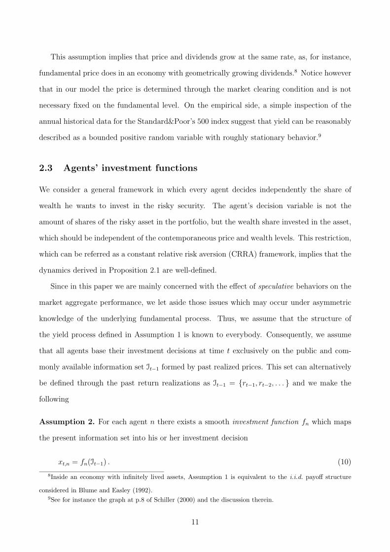
This assumption implies that price and dividends grow at the same rate, as, for instance,

fundamental price does in an economy with geometrically growing dividends.8 Notice however

that in our model the price is determined through the market clearing condition and is not

necessary fixed on the fundamental level. On the empirical side, a simple inspection of the

annual historical data for the Standard&Poor’s 500 index suggest that yield can be reasonably

described as a bounded positive random variable with roughly stationary behavior.9

2.3 Agents’ investment functions

We consider a general framework in which every agent decides independently the share of

wealth he wants to invest in the risky security. The agent’s decision variable is not the

amount of shares of the risky asset in the portfolio, but the wealth share invested in the asset,

which should be independent of the contemporaneous price and wealth levels. This restriction,

which can be referred as a constant relative risk aversion (CRRA) framework, implies that the

dynamics derived in Proposition 2.1 are well-defined.

Since in this paper we are mainly concerned with the effect of speculative behaviors on the

market aggregate performance, we let aside those issues which may occur under asymmetric

knowledge of the underlying fundamental process. Thus, we assume that the structure of

the yield process defined in Assumption 1 is known to everybody. Consequently, we assume

that all agents base their investment decisions at time t exclusively on the public and com-

monly available information set It−1 formed by past realized prices. This set can alternatively

be defined through the past return realizations as It−1 = {rt−1, rt−2, . . . } and we make the

following

Assumption 2. For each agent n there exists a smooth investment function fn which maps

the present information set into his or her investment decision

xt,n = fn(It−1) . (10)

8Inside an economy with infinitely lived assets, Assumption 1 is equivalent to the i.i.d. payoff structure

considered in Blume and Easley (1992).9See for instance the graph at p.8 of Schiller (2000) and the discussion therein.

11

The function fn gives a complete description of the investment decision of the n-th agent

who adapts to observed price fluctuations. The knowledge about the yield process is not

explicitly inserted in the information set but can be considered embedded in the functional

form of fn.

Assumption 2 is strictly related to the “smooth” learning hypothesis described in Grand-

mont (1998). It is compatible with a number of different learning processes based on common

information, as for instance the Bayesian learning, or, more generally, the adaptive models

explored inside the EF literature (Blume and Easley, 1992; Hens and Schenk-Hoppe, 2005).

Indeed, the investment choice in (10) can be thought as the result of two separate steps. In

the first step agent n, using a set of estimators or “expectation functions” (Grandmont, 1998)

{gn,1, gn,2, . . . }, forms his prediction about the behavior of future prices, θn,j = gn,j(It−1),

where θ.,j stands for some statistics of the returns distribution at time t + 1, e.g. the average

return, the expected variance or the probability that a given return threshold will be crossed.

Then, using a choice function hn defined in terms of these expectations, the agent computes

the fraction of wealth invested in the risky asset xt+1,n = hn(θn,1, θn,2, . . . ). As a result, the

investment function fn becomes a composition of a set of estimators {gn,·} and an individual

choice function hn. The choice function can be derived from some optimization procedure (as

the maximization of expected utility under uncertainty) or, more generally, can reflect a sat-

isfying behavior. The expectation functions g’s can account for the outcomes of fundamental

and technical valuation, widely used both in trading practices observed in real markets and in

the HAMs. The present framework is indeed able to account for a wide spectrum of behavioral

assumptions. An example is provided in Appendix B where we briefly discuss how a myopic

utility maximization framework, widely adopted by the HAM literature, can be treated in

terms of expectation and choice functions. Another example is the model we developed in

Anufriev, Bottazzi, and Pancotto (2006) (the predecessor of this paper), in which adaptive

agents decide their investment shares on the basis of exponentially weighted moving averages

of past returns and their variance. Our Assumption 2 generalizes such behaviour by allow-

ing agents to map the past return history into the future investment choice, using whatever

12

smooth function they like. Using the terminology coined by Herbert Simon (Simon, 1976),

in this paper we consider generic procedurally rational traders whose investment functions are

the collective description of preferences, beliefs and implied actions.

Under Assumption 1, the dynamics in terms of price return, wealth shares and investment

shares are described by (7), (9) and (10). In order to analyze a finite-dimensional system

we restrict each agent n to base his decision on the past Ln price returns. Without loss of

generality we can assume that the “memory span” is the same for all traders and denote it by

L. For the following discussion L must be finite, but can be arbitrarily large.

2.4 Procedurally Consistent Equilibria

The “rational expectations” approach (Muth, 1961; Lucas, 1978) postulating that the dynam-

ics generated by the actions of an agent should be consistent with his a priori expectations

about the dynamics itself, is too restrictive for a framework with heterogeneous, procedurally

rational agents. A suitable concept for such framework would be an “adaptive procedural

rationality” under which agents’ actions generate dynamics which are in turn consistent with

these co-evolving actions. In this paper we focus on the emergence of equilibria of this kind,

defined as situations in which agents are have no incentive to review their choices. In the

setup outlined in Sections 2.1 and 2.2 the agents choose the wealth share x to invest in the

risky asset. Consequently we apply the following

Definition 2.1. Procedurally Consistent Equilibria (PCE) are the trajectories of the system

defined by (7) and (8) (or, equivalently, by (7) and (9)) with fixed investment shares xt,n = x∗n

and stationary wealth distribution ϕt,n = ϕ∗n for all n and t.

At the PCE agents are not changing their actions, and, at the same time, the aggregate

dynamics is consistent with the procedures agents use to decide their positions in the market.

While the consistency requirement seems intuitive, the assumption of constant actions requires

some justification. It is, for instance, at odds with complex dynamics emerging in many

HAMs, e.g. Day and Huang (1990), Chiarella (1992) or Brock and Hommes (1998), where one

13

observes cyclic or even chaotic motion of individual agents’ wealth and portfolios. Indeed,

our interest lies not in the global dynamics of a market with a few agents having stylized

behaviors, but in the investigation, under general assumptions, of the local properties of the

feasible PCE. Moreover, the situation in which an agent changes his position each period in

a chaotic manner does not only seems unrealistic, but, in our opinion, can hardly play a role

in the generalization of the notion of equilibrium for multi-agent setting. For instance, if a

forecasting agent observes persistent mistakes (periodic or quasi-periodic) in his prediction

of future market dynamics, he will probably adopt new forecasting procedures. The new

procedures would make his investment decision different and, ultimately, perturb the system

away from the previous trajectory. As long as a minimal evolutionary pressure is put on the

system, so that agents can revise their strategies if they led to incorrect expectations, any

equilibrium whose dynamics is not consistent with the actions of agents is likely to have a

transitory nature.

In what follows any use of the term “equilibrium” refers to the specific notion of equilibrium

introduced by Definition 2.1.

3 Single Agent Case

We start with the analysis of the very special situation in which a single agent operates in the

market. The main reason to perform this analysis rests in its relevance for the multi-agent

case, as we will see in the next Section. In particular, some type of the generic equilibrium

in the setting with N heterogeneous traders requires, as necessary condition for stability, the

stability of a suitably defined single agent equilibrium.

This Section starts laying down the dynamics of the single agent economy as a multidimen-

sional dynamical system of difference equations of the first order. All possible steady-states

of the system are identified and their stability studied using the associated characteristic

polynomial.

14

3.1 Dynamical system

In the case of one single agent the evolution of wealth shares in (8) is trivial and can be ignored.

As a consequence, the whole system can be described with only L + 1 variables representing

the present investment choice and the L past returns. We denote the price return at time t− l

as rt,l, so that the system reads

xt+1 = f(rt,0, rt,1, . . . , rt,L−1

)

rt+1,0 = R(f(rt,0, rt,1, . . . , rt,L−1

), xt, et

)

rt+1,1 = rt,0

...

rt+1,L−1 = rt,L−2 .

(11)

The function R in the right hand-side of (7) is defined as

R(x′, x, e) =x′ − x + e x′ x

(1− x′) x, (12)

where x, x′ and e denote the previous period investment choice, the current (contemporaneous

with return) investment choice and the dividend yield, respectively.

The system (11) depends on the noise component et which, according to Assumption 1, is

an i.i.d. random variable. In the following analysis we substitute the yield realizations {et}by their mean value e considering the deterministic skeleton of (11). The resulting system

describes, in a sense, the “average” of the stochastic dynamics.10 Once referred to the deter-

ministic skeleton, the set of Procedurally Consistent Equilibria introduced in Definition 2.1

reduces to a set of fixed points of (11). Indeed, from (12), if the investment choice x is

not changing over time, then x = x′, and price returns are also constant. The next section

investigates whether it is possible to characterize all the fixed points of (11).

10This substitution is in general dangerous, as small random shocks could accumulate along a trajectory so

that their final effect on the system dynamics becomes huge. This is however not the case when one considers

asymptotically stable fixed points, as we will do later. In this case, as long as random shocks are sufficiently

small, the dynamics of the stochastic system is bounded in a neighborhood of the fixed point of the associated

deterministic skeleton.

15

3.2 Equilibrium market curve

It turns out that independently of agent’s behavior, all possible equilibria belong to a one-

dimensional curve, the Equilibrium Market Curve. The next definition introduces the locus of

equilibria, while the following proposition, which characterizes the equilibria of (11), clarify

its role.

Definition 3.1. The Equilibrium Market Curve (EMC) is the function l(r) defined as

l(r) =r

e + r. (13)

Let x∗ denote the agent’s wealth share invested in the risky asset at equilibrium and let r∗

be the equilibrium return (equal to the returns for all lags). One has the following

Proposition 3.1. Let x∗ = (x∗; r∗, . . . , r∗) be a fixed point of the deterministic skeleton of

(11). Then

(i) the equilibrium return r∗ and the equilibrium investment share x∗ satisfy

l(r∗) = f(r∗, . . . , r∗) , x∗ = f(r∗, . . . , r∗) . (14)

(ii) at the fixed point x∗ prices are positive if either x∗ < 1 or x∗ ≥ 1/(1− e).

(iii) in x∗ the growth rate of agent’s wealth is equal to the price return r∗.

Proof. See appendix C.

The first statement in the previous Proposition justifies the introduction of the Equilibrium

Market Curve in Definition 3.1. Indeed, according to (14) all fixed points of the dynamics can

be found as the intersections of the EMC with the symmetrization of function f , i.e. with the

restriction of this function to the one-dimensional subspace defined as r0 = r1 = · · · = rL−1.

The main reason for such a simple characterization of equilibria is the underlying requirement

of consistency between self-fulfilling agent’s choice and the resulting dynamics. The EMC is

the locus of points where agents’ expectation formation mechanism is compatible with the

intertemporal relation governing market dynamics.

16

-e- 0r*-e-0

r*-1

-0.5

0

0.5

1

1.5

r0

r1

Inve

stm

ent S

hare

Rescaled Price Return

Equilibrium Market Curve

0

1

-1 -e- 0

S1

U1

S2

U2

E

I

II

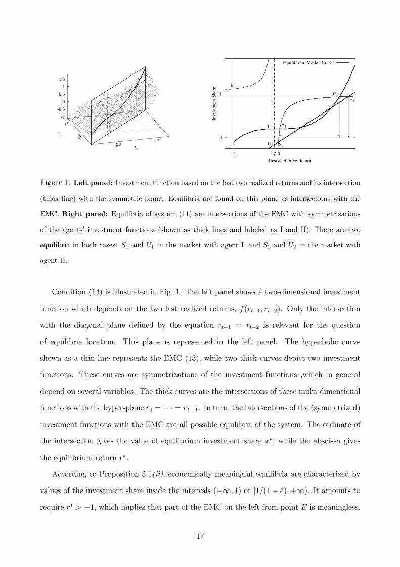
Figure 1: Left panel: Investment function based on the last two realized returns and its intersection

(thick line) with the symmetric plane. Equilibria are found on this plane as intersections with the

EMC. Right panel: Equilibria of system (11) are intersections of the EMC with symmetrizations

of the agents’ investment functions (shown as thick lines and labeled as I and II). There are two

equilibria in both cases: S1 and U1 in the market with agent I, and S2 and U2 in the market with

agent II.

Condition (14) is illustrated in Fig. 1. The left panel shows a two-dimensional investment

function which depends on the two last realized returns, f(rt−1, rt−2). Only the intersection

with the diagonal plane defined by the equation rt−1 = rt−2 is relevant for the question

of equilibria location. This plane is represented in the left panel. The hyperbolic curve

shown as a thin line represents the EMC (13), while two thick curves depict two investment

functions. These curves are symmetrizations of the investment functions ,which in general

depend on several variables. The thick curves are the intersections of these multi-dimensional

functions with the hyper-plane r0 = · · · = rL−1. In turn, the intersections of the (symmetrized)

investment functions with the EMC are all possible equilibria of the system. The ordinate of

the intersection gives the value of equilibrium investment share x∗, while the abscissa gives

the equilibrium return r∗.

According to Proposition 3.1(ii), economically meaningful equilibria are characterized by

values of the investment share inside the intervals (−∞, 1) or [1/(1− e), +∞). It amounts to

require r∗ > −1, which implies that part of the EMC on the left from point E is meaningless.

17

On the remaining part of the Curve one can distinguish between three qualitatively different

scenarios.

In the first scenario, when r∗ ∈ [−1,−e), the return is negative and, hence, rescaled price

pt of the risky asset decreases to 0. The wealth of the agent is positive at any moment of time

and is eventually vanishing. The agent possesses the total supply of the risky asset, while his

own amount of the numeraire is negative. Thus, the agent has to borrow money in order to

keep his relatively high demand for the risky asset. Due to the decrease in the agent’s wealth,

this demand is insufficient to generate high (not even positive) returns.

In the second scenario, when r∗ ∈ (−e, 0), the capital gain on the risky asset is negative

and the price of the asset decreases. However, the contribution from the dividend makes

the gross return r∗ + e positive. Furthermore, agent has to have negative wealth (has to be

indebted) and, at the same time, has to borrow money in order to keep the demand of the

asset positive.11 The agent possesses the total supply of the risky asset and a negative amount

of the numeraire. From Proposition 3.1(iii) it follows that the dividend payment allows the

agent’s wealth to increase to 0. Equilibrium S2 for agent II in the left panel of Fig. 1 is of

such kind.

Finally, in the third scenario, when the rescaled return is positive, the price pt of the asset

increases. Agent has a positive amount of the numeraire and his total wealth is positive and

increasing. Such a situation is observed in equilibria S1, U1 and U2.

What can be said about the dynamics of unscaled price Pt in all these three scenarios? To

answer this question it is important to bear in mind the following relation between the scaled

return rt and return Rt in terms of unscaled price:

1 + Rt = (1 + rt) (1 + rf ) .

Therefore, in the third scenario, where the rescaled price increases, the unscaled price also

increases with a higher rate. Conversely, in the first and second scenarios, even if the rescaled

11In general, to guarantee the positiveness of the price at the initial period one has to choose initial wealth

appropriately. Since p0 = x∗w0, for positive x∗ the initial (and consequent) agent’s wealth is positive, while

for negative x∗ the wealth is negative.

18

price is decreasing, the unscaled price may increase due to high enough risk-free interest rate.

To conclude our discussion about equilibrium properties notice that in all possible equilibria

there exists a non-zero equity premium, i.e. a difference between the total return of the riskless

and the risky asset given by

Pt+1 − Pt + Dt+1

Pt

− rf =e (1 + rf )

1− x∗. (15)

The equity premium, which is empirically observed in real markets (Mehra and Prescott,

1985), can be explained, within the classical paradigm, as a monetary incentive required by an

optimizing risk-averse representative agent to hold the risky asset. In our framework, instead,

the risk premium is endogenously generated by the feedback effect from market return to

agent’s wealth and the reinvestment of the latter. Consequently, the equity premium increases

with the dividend yield (1 + rf )e and with the propensity of agent to invest in the risky asset,

x∗.

3.3 Stability of single-agent equilibria

The stability conditions are derived from the analysis of the roots of the characteristic polyno-

mial associated with the Jacobian of system (11) computed at equilibrium. The characteristic

polynomial does, in general, depend on the behavior of the individual investment function f

in an infinitesimal neighborhood of the equilibrium x∗. This dependence can be summarized

with the help of the following

Definition 3.2. The stability polynomial P (µ) of the investment function f in x∗ is

Pf (µ) =∂f

∂r0

µL−1 +∂f

∂r1

µL−2 + · · ·+ ∂f

∂rL−2

µ +∂f

∂rL−1

, (16)

where all the derivatives are computed in (r∗, . . . , r∗).

Using the previous definition, the stability conditions can be formulated in terms of the

equilibrium return r∗, and of the slope of the EMC at equilibrium

l′(r∗) =e

(e + r∗)2.

The following applies

19

Proposition 3.2. The fixed point x∗ = (x∗; r∗, . . . , r∗) of system (11) is (locally) asymptoti-

cally stable if all the roots of the polynomial

Q(µ) = µL+1 − Pf (µ)

r∗ l′(r∗)

((1 + r∗

)µ− 1

)(17)

are inside the unit circle. The equilibrium x∗ is unstable if at least one of the roots of Q(µ)

lies outside the unit circle.

Proof. The condition above is a direct consequence of the characteristic polynomial of the

Jacobian matrix at equilibrium. See Appendix D for a derivation.

Once the investment function f is known, the polynomial Pf (µ) and, in turn, the polyno-

mial Q(µ) can be explicitly derived. The analysis of the L + 1 roots of Q(µ) (usually called

multipliers) reveals the role of the different parameters in stabilizing a given equilibrium.

3.4 Examples of single-agent system

Since the explicit expression for the roots of (17) cannot, in general, be derived even for rel-

atively simple investment functions, the analytical study of the effect of different parameters

is often unfeasible and one has to rely on numerical investigations. Mainly for illustrative

purposes we present below three relatively simple cases where analytical results are, to some

extent, available. Inspired by models already discussed in the literature, we show how Propo-

sitions 3.1 and 3.2 can be applied to obtain rather general results about the effect of different

behavioral assumptions. The reader is referred to Appendix E for the derivation of results

and for further discussions.

Example 1. Agent with short memory, L = 1.

Consider an agent with a memory spanning a single lag, i.e. whose present investment share

depends only on the last realized return, xt+1 = f(rt). This is, for instance, the case of an

agent who simply predicts the next price return to be equal to the last realized return. In this

case, the stability polynomial is simply Pf = f ′(r∗). Applying the general result obtained in

Propositions E.1 and E.2, one gets

20

Proposition 3.3. The fixed point x∗ = (x∗; r∗) of system (11) with L = 1 is (locally) asymp-

totically stable if

f ′(r∗)l′(r∗)

1

r∗< 1 ,

f ′(r∗)l′(r∗)

< 1 andf ′(r∗)l′(r∗)

2 + r∗

r∗> −1 . (18)

The fixed point exhibits a Neimark-Sacker, fold or flip bifurcation if the first, second or third

inequality in (18) turns to equality, respectively.

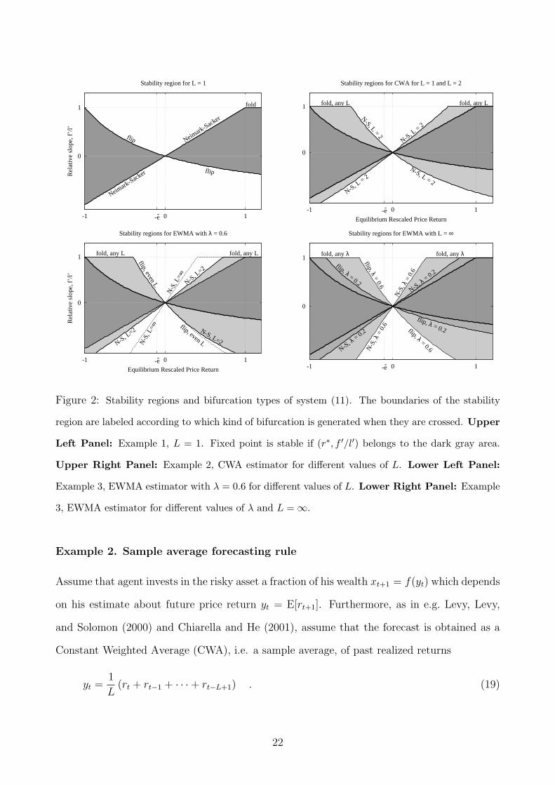
The stability region S defined by the three inequalities in (18) is shown as a dark area in

the upper left panel of Fig. 2 in coordinates r∗ and f ′(r∗)/l′(r∗). The second coordinate is

the relative slope of the investment function at equilibrium with respect to the slope of the

Equilibrium Market Curve. The boundaries of the stability region are labeled as “Neimark-

Sacker”, “flip” and “fold” depending on the type of bifurcation undertaken by the system when

a particular boundary is crossed (e.g. ”Neimark-Sacker” curve corresponds to those points

where two complex conjugated multipliers cross the unit circle). Notice that if the slope of

f at equilibrium is zero, that is, the investment function is locally constant, the equilibrium

is always stable. A constant investment function represent an agent whose portfolio choice

is insensitive to price variations. An increase in the sensitivity to price, that is of the slope

of f , would ultimately lead to system instability. Since for r > 0 the slope of the EMC is

decreasing, the larger the value of r, the lower is the minimal strength of agent reaction to

price fluctuations necessary to destabilize the equilibrium.

As an example of application of Proposition 3.3 consider the investment functions drawn

in the left panel of Fig. 1. Assume that the memory span of each agent L is equal to one. In

this case, both equilibrium U1 for agent I and U2 for agent II are unstable, since the second

inequality in (18) is violated. On the contrary, S1 is (presumably) a stable equilibrium, since

the slope of the investment function I in that point is positive and very small. If this slope

would increase, the equilibrium S1 will lose its stability through a Neimark-Sacker bifurcation

(c.f. upper left panel of Fig. 2). Conversely, the negative value of the equilibrium return r∗ in

S2 implies that an increase of the slope of the investment function II in that point would lead

to a flip bifurcation.

21

Rel

ativ

e sl

ope,

f’/

l’

Stability region for L = 1

Neimark

-Sacker

fold

Neimark

-Sacker

flip

flip

0

1

-1 -e- 0 1 Equilibrium Rescaled Price Return

Stability regions for CWA for L = 1 and L = 2

0

1

-1 -e- 0 1

fold, any L fold, any L

N-S, L = 2

N-S, L

= 2

N-S, L = 2

N-S, L = 2

Rel

ativ

e sl

ope,

f’/

l’

Equilibrium Rescaled Price Return

Stability regions for EWMA with λ = 0.6

0

1

-1 -e- 0 1

fold, any L fold, any L

N-S

, L=∞

N-S

, L=∞

N-S, L=2

N-S, L

=2

N-S, L=2

flip, even L

flip, even L

Stability regions for EWMA with L = ∞

fold, any λ fold, any λ

N-S

, λ =

0.6

N-S

, λ =

0.6

flip, λ = 0.6

flip, λ = 0.6

0

1

-1 -e- 0 1

N-S, λ = 0.2

N-S, λ = 0.2flip, λ = 0.2

flip, λ = 0.2

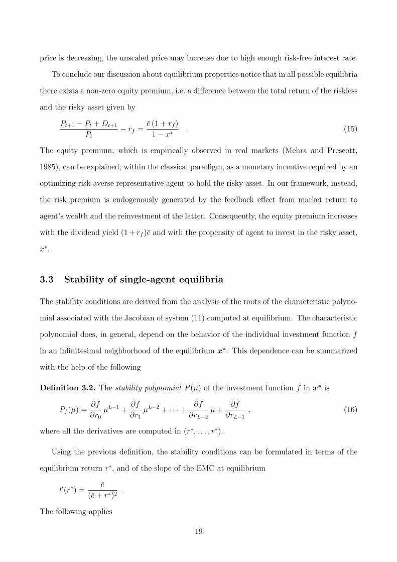
Figure 2: Stability regions and bifurcation types of system (11). The boundaries of the stability

region are labeled according to which kind of bifurcation is generated when they are crossed. Upper

Left Panel: Example 1, L = 1. Fixed point is stable if (r∗, f ′/l′) belongs to the dark gray area.

Upper Right Panel: Example 2, CWA estimator for different values of L. Lower Left Panel:

Example 3, EWMA estimator with λ = 0.6 for different values of L. Lower Right Panel: Example

3, EWMA estimator for different values of λ and L = ∞.

Example 2. Sample average forecasting rule

Assume that agent invests in the risky asset a fraction of his wealth xt+1 = f(yt) which depends

on his estimate about future price return yt = E[rt+1]. Furthermore, as in e.g. Levy, Levy,

and Solomon (2000) and Chiarella and He (2001), assume that the forecast is obtained as a

Constant Weighted Average (CWA), i.e. a sample average, of past realized returns

yt =1

L(rt + rt−1 + · · ·+ rt−L+1) . (19)

22

The parameter L defines the length of agent’s memory, that is how many past realizations

are considered to obtain an estimation about future return. The parameter L clearly acts

as a smoothing factor on the agent’s behavior: the larger its value, the more the time steps

needed for a new trend in returns to be reflected in agent’s forecast. We will apply the result

of the previous sections to understand how different memory lengths affect the behavior of the

market.

Since at equilibrium the forecast coincides with the return, yt = r∗, the stability polynomial

reads

Pf (µ) = f ′(r∗)1

L

µL − 1

µ− 1. (20)

By plugging this expression in (17) one can in principle compute the L + 1 multipliers of

the polynomial Q(µ) for the CWA agent. The region of the parameter space where all these

multipliers are inside the unit circle is the stability region of the system. Let’s denote it with

SL, since it clearly depends on the memory length L. As before, this region can be represented

using the (r∗, f ′/l′) coordinates system.

We study the effect on the system of different memory lengths by analyzing the dependence

of the stability region on the parameter L. When L = 1 we are back to the previous Example.

The stability region S1 is shown as a dark gray area in the upper right panel of Fig. 2.

Irrespectively on the value of L, the boundary associated with a fold bifurcation is given by

the line f ′/l′ = 1. Notice that a flip bifurcation is possible only for odd values of L. The

stability region for L = 2 can be obtained analytically and is depicted in the upper right panel

of Fig. 2 as the union of the dark and light gray areas. Since locally horizontal investment

functions always lead to stable equilibria, the points of the horizontal axes lie in the stability

region. This region increases with L and for large enough values of the memory parameter,

any fixed point with f ′/l′ < 1 becomes stable.

Summarizing, a large memory span L has a stabilizing effect on the dynamics of the

system. However, if the agent investment function f is too steep, that is if she overreacts

to price fluctuations by a too large readjustment of her portfolio position, then the market

is unstable, irrespectively of the value of L. Referring again to the EMC plot in Fig. 1, for

23

investment functions based on CWA estimators, equilibria U1 and U2 are always unstable.

Conversely, both equilibria S1 and S2 will become stable for large enough value of L.

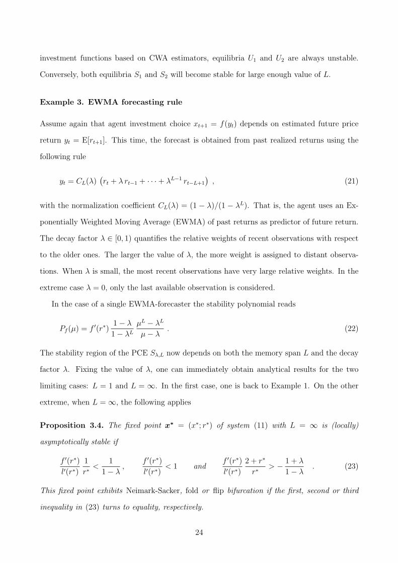
Example 3. EWMA forecasting rule

Assume again that agent investment choice xt+1 = f(yt) depends on estimated future price

return yt = E[rt+1]. This time, the forecast is obtained from past realized returns using the

following rule

yt = CL(λ)(rt + λ rt−1 + · · ·+ λL−1 rt−L+1

), (21)

with the normalization coefficient CL(λ) = (1 − λ)/(1 − λL). That is, the agent uses an Ex-

ponentially Weighted Moving Average (EWMA) of past returns as predictor of future return.

The decay factor λ ∈ [0, 1) quantifies the relative weights of recent observations with respect

to the older ones. The larger the value of λ, the more weight is assigned to distant observa-

tions. When λ is small, the most recent observations have very large relative weights. In the

extreme case λ = 0, only the last available observation is considered.

In the case of a single EWMA-forecaster the stability polynomial reads

Pf (µ) = f ′(r∗)1− λ

1− λL

µL − λL

µ− λ. (22)

The stability region of the PCE Sλ,L now depends on both the memory span L and the decay

factor λ. Fixing the value of λ, one can immediately obtain analytical results for the two

limiting cases: L = 1 and L = ∞. In the first case, one is back to Example 1. On the other

extreme, when L = ∞, the following applies

Proposition 3.4. The fixed point x∗ = (x∗; r∗) of system (11) with L = ∞ is (locally)

asymptotically stable if

f ′(r∗)l′(r∗)

1

r∗<

1

1− λ,

f ′(r∗)l′(r∗)

< 1 andf ′(r∗)l′(r∗)

2 + r∗

r∗> − 1 + λ

1− λ. (23)

This fixed point exhibits Neimark-Sacker, fold or flip bifurcation if the first, second or third

inequality in (23) turns to equality, respectively.

24

Proof. The result can be obtained rigorously through reduction of infinite-dimensional system

(11) to the two-dimensional one, using the recursive relation available for the EWMA estimator

in case L = ∞. See Anufriev, Bottazzi, and Pancotto (2006). In Appendix E we sketch an

alternative proof.

The conditions in (23) can be used to establish the boundaries of the stability region Sλ,∞.

Three examples for different values of λ (S0,∞, S0.2,∞ and S0.6,∞) are depicted on the lower

right panel of Fig. 2. For λ = 0 the stability region S0,∞ is the same as in Example 1, and

is shown as a dark gray area. If λ = 0.2 it expands and becomes the union of the dark and

semi-dark gray areas. When λ = 0.6 the region expands further and contains the light gray

areas in addition. As expected, an increase of the decay factor brings stability to the system.

For the intermediate case, when L is greater than one, but finite, analytic results are

limited. The case L = 2 is analyzed in Appendix E, and the corresponding bifurcation curves

are shown, for λ = 0.6, in the lower left panel of Fig. 2. The stability region S.6,1 is shown as a

dark gray area. The region S.6,2 is the union of the dark and light gray areas. The boundaries

for L = ∞ are shown as dotted lines.

Differently from the L = ∞ case, for equilibria with r∗ > 0 investment functions with a

negative slope generate Neimark-Sacker (and not flip) bifurcations. The boundary leading to

the fold bifurcation, on the contrary, remains the same for any L and is given by the line

f ′/l′ = 1. Finally, the boundary leading to the flip bifurcation depends on whether L is even

or odd. For even L, the locus is invariant and coincides with the corresponding boundary for

L = ∞. When L is odd, the locus depends on L and converges point-wise to the boundary

of Sλ,∞ when L → ∞. This result implies that the expansion of the stability region is not

monotone in the memory span.

As Proposition 3.4 guarantees, an increase in the memory span L ultimately brings stability

to all fixed points belonging to the interior of Sλ,∞. Since for a given λ this region does not cover

the whole parameter space (r∗, f ′/l′), not all fixed points can be stabilized by a sole increase

of L. One can then ask whether unstable fixed points become stable by an appropriate choice

of the decay factor λ. The general answer to this question is no, since the condition f ′/l′ < 1

25

has to be satisfied. However, all fixed points for which this condition holds can be stabilized

through an increase of λ. Indeed, from (23) it follows that the region Sλ,∞ enlarges with λ and

for λ → 1 contains all equilibria with f ′(r∗)/l′(r∗) < 1 (c.f. the lower right panel of Fig. 2).

Let us exemplify our findings, referring again to the EMC plot in Fig. 1. For investment

functions based on EWMA estimators, equilibria U1 and U2 cannot be stabilized neither by

increasing the memory span L, nor by increasing the decay factor λ. Conversely, both equilibria

S1 and S2 will become stable for large enough value of λ and an appropriate L.

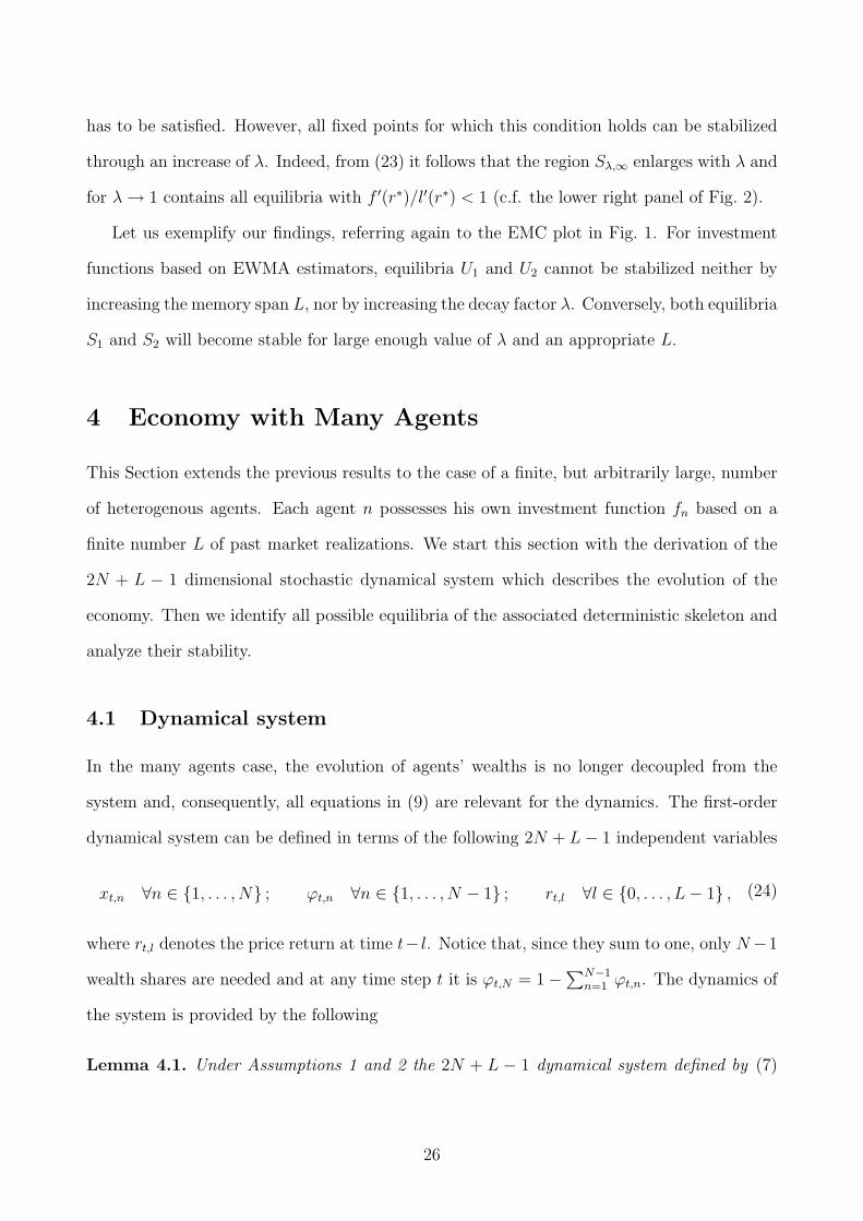
4 Economy with Many Agents

This Section extends the previous results to the case of a finite, but arbitrarily large, number

of heterogenous agents. Each agent n possesses his own investment function fn based on a

finite number L of past market realizations. We start this section with the derivation of the

2N + L − 1 dimensional stochastic dynamical system which describes the evolution of the

economy. Then we identify all possible equilibria of the associated deterministic skeleton and

analyze their stability.

4.1 Dynamical system

In the many agents case, the evolution of agents’ wealths is no longer decoupled from the

system and, consequently, all equations in (9) are relevant for the dynamics. The first-order

dynamical system can be defined in terms of the following 2N + L− 1 independent variables

xt,n ∀n ∈ {1, . . . , N} ; ϕt,n ∀n ∈ {1, . . . , N − 1} ; rt,l ∀l ∈ {0, . . . , L− 1} , (24)

where rt,l denotes the price return at time t− l. Notice that, since they sum to one, only N−1

wealth shares are needed and at any time step t it is ϕt,N = 1−∑N−1n=1 ϕt,n. The dynamics of

the system is provided by the following

Lemma 4.1. Under Assumptions 1 and 2 the 2N + L − 1 dynamical system defined by (7)

26

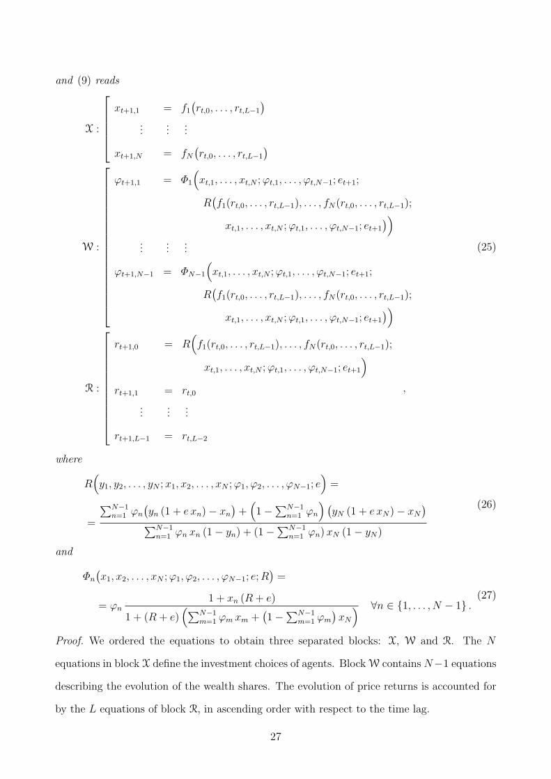
and (9) reads

X :

xt+1,1 = f1

(rt,0, . . . , rt,L−1

)

......

...

xt+1,N = fN

(rt,0, . . . , rt,L−1

)

W :

ϕt+1,1 = Φ1

(xt,1, . . . , xt,N ; ϕt,1, . . . , ϕt,N−1; et+1;

R(f1(rt,0, . . . , rt,L−1), . . . , fN(rt,0, . . . , rt,L−1);

xt,1, . . . , xt,N ; ϕt,1, . . . , ϕt,N−1; et+1

))

......

...

ϕt+1,N−1 = ΦN−1

(xt,1, . . . , xt,N ; ϕt,1, . . . , ϕt,N−1; et+1;

R(f1(rt,0, . . . , rt,L−1), . . . , fN(rt,0, . . . , rt,L−1);

xt,1, . . . , xt,N ; ϕt,1, . . . , ϕt,N−1; et+1

))

(25)

R :

rt+1,0 = R(f1(rt,0, . . . , rt,L−1), . . . , fN(rt,0, . . . , rt,L−1);

xt,1, . . . , xt,N ; ϕt,1, . . . , ϕt,N−1; et+1

)

rt+1,1 = rt,0

......

...

rt+1,L−1 = rt,L−2

,

where

R(y1, y2, . . . , yN ; x1, x2, . . . , xN ; ϕ1, ϕ2, . . . , ϕN−1; e

)=

=

∑N−1n=1 ϕn

(yn (1 + e xn)− xn

)+

(1−∑N−1

n=1 ϕn

) (yN (1 + e xN)− xN

)∑N−1

n=1 ϕn xn (1− yn) + (1−∑N−1n=1 ϕn) xN (1− yN)

(26)

and

Φn

(x1, x2, . . . , xN ; ϕ1, ϕ2, . . . , ϕN−1; e; R

)=

= ϕn1 + xn (R + e)

1 + (R + e)(∑N−1

m=1 ϕm xm +(1−∑N−1

m=1 ϕm

)xN

) ∀n ∈ {1, . . . , N − 1} .(27)

Proof. We ordered the equations to obtain three separated blocks: X, W and R. The N

equations in block X define the investment choices of agents. Block W contains N−1 equations

describing the evolution of the wealth shares. The evolution of price returns is accounted for

by the L equations of block R, in ascending order with respect to the time lag.

27

The block X is directly obtained from the definition of the investment functions. The first

equation of block R is (7) rewritten in terms of variables (24) using (26) and (5), while the

remaining equations are just the result of a “lag” operation. Notice that (26) reduces to (12)

in the case of one agent. Finally, the evolution of wealth shares described by block W is

obtained from (9) expanding the notation introduced in (5). Due to the presence of function

R in the last expression, all functions Φn depend on the same set of variables as R.

The rest of this Section is devoted to the analysis of the deterministic skeleton of (25).

We replace the yield realizations {et} by their mean value e and analyze the procedurally

consistent equilibria, the is the fixed points, of the resulting deterministic system.

4.2 Determination of equilibria

The characterization of fixed points of system (25) is in many respects similar to the single

agent case discussed above. Let x∗ = (x∗1, . . . , x∗N ; ϕ∗1, . . . , ϕ

∗N−1; r

∗, . . . , r∗) denotes a fixed

point where r∗ is the equilibrium return, and x∗n and ϕ∗n stand for the equilibrium value of

the investment function and the equilibrium wealth share of agent n, respectively. Let us

introduce the following

Definition 4.1. Agent n is said to survive in x∗ if his equilibrium wealth share is different

from zero, ϕ∗n 6= 0. Agent n is said to dominate the economy if he is the only survivor,

i.e. ϕ∗n = 1.

One can recognize the parallel between our definition above and the frameworks in DeLong,

Shleifer, Summers, and Waldmann (1991) and Blume and Easley (1992). We adopt here the

deterministic version of the concepts of survival and dominance used in that papers. The

following statement characterizes all possible equilibria of system (25).

Proposition 4.1. Let x∗ be a PCE of the deterministic skeleton of system (25). Then equi-

librium investment shares are defined according to

x∗n = fn(r∗, . . . , r∗) ∀n ∈ {1, . . . , N} , (28)

and three mutually exclusive cases are possible:

28

(i) Single survivor. In x∗ only one agent survives and, therefore, dominates the economy.

Without loss of generality we can assume this agent to be agent 1 so that ϕ∗1 = 1 and all

other equilibrium wealth shares are equal to zero.

The equilibrium return r∗ is determined as the solution of

l(r∗) = f1(r∗, . . . , r∗) , (29)

and is equal to the equilibrium wealth growth rate of the survivor.

(ii) Non-generic many survivors. In x∗ more than one agent survives. Without loss

of generality one can assume that the agents with non-zero wealth shares are the first k

agents (with k > 1) so that the equilibrium wealth shares satisfy

ϕ∗n = 0 ∀n > k andk∑

n=1

ϕ∗n = 1 . (30)

The equilibrium return r∗ must simultaneously satisfy the following set of k equations

l(r∗) = fn(r∗, . . . , r∗) ∀n ∈ {1, . . . , k} , (31)

implying that the first k agents have the same equilibrium investment share x∗1¦k. The

wealth growth rates of all survivors are equal to r∗.

(iii) Generic many survivors. In x∗ the equilibrium return r∗ = −e. The wealth shares

of agents satisfy the two following conditions

N∑n=1

x∗nϕ∗n = 0 and

N∑n=1

ϕ∗n = 1 . (32)

The wealth growth rates of all agents are equal to 0.

Proof. See appendix F.

The difference between items (i) and (ii) is that in the first case, when a single agent

survives, Proposition 4.1 defines a precise value for each component (x∗, ϕ∗ and r∗) of the

equilibrium x∗, so that a single point is uniquely determined. In the second case, on the

contrary, there is a residual degree of freedom in the definition of the equilibrium: while the

29

price return r∗ and the investment share x∗ are uniquely defined, the only requirement on the

equilibrium wealth shares of the surviving agents, ϕ∗n (for n ≤ k), is the fulfillment of the

second equality in (30). Consequently we have

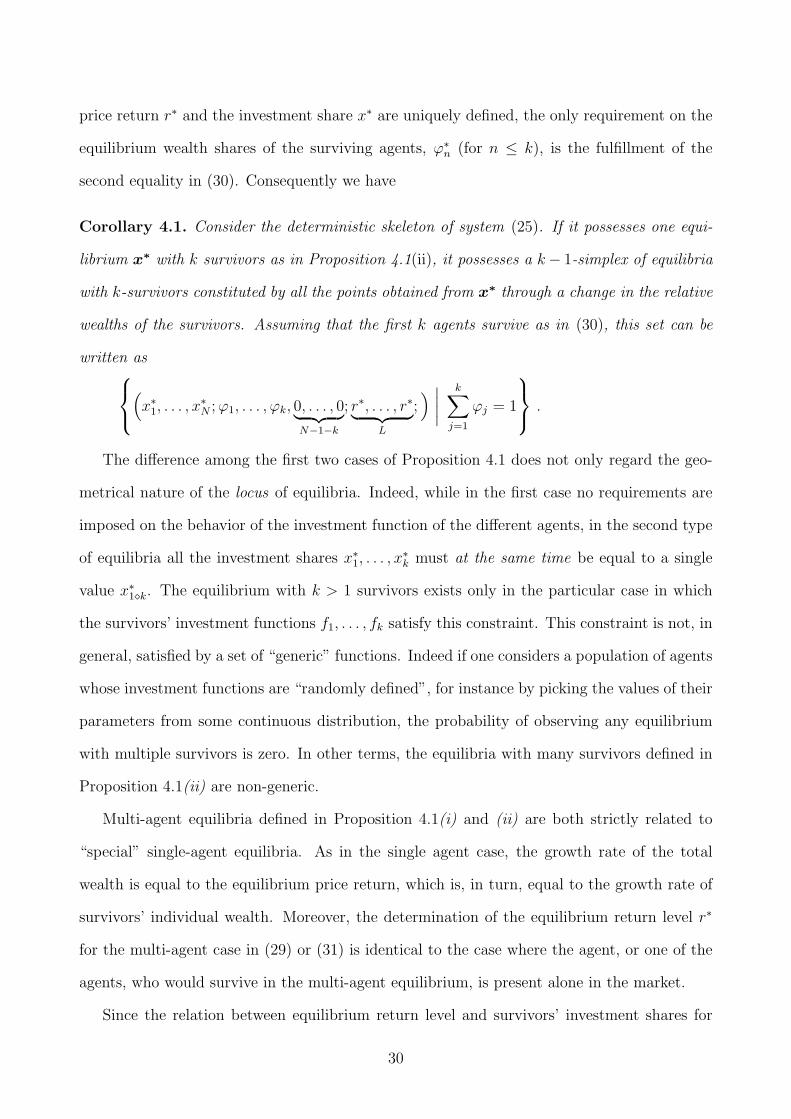
Corollary 4.1. Consider the deterministic skeleton of system (25). If it possesses one equi-

librium x∗ with k survivors as in Proposition 4.1(ii), it possesses a k− 1-simplex of equilibria

with k-survivors constituted by all the points obtained from x∗ through a change in the relative

wealths of the survivors. Assuming that the first k agents survive as in (30), this set can be

written as

(x∗1, . . . , x

∗N ; ϕ1, . . . , ϕk, 0, . . . , 0︸︷︷︸

N−1−k

; r∗, . . . , r∗︸︷︷︸L

;) ∣∣∣∣

k∑j=1

ϕj = 1

.

The difference among the first two cases of Proposition 4.1 does not only regard the geo-

metrical nature of the locus of equilibria. Indeed, while in the first case no requirements are

imposed on the behavior of the investment function of the different agents, in the second type

of equilibria all the investment shares x∗1, . . . , x∗k must at the same time be equal to a single

value x∗1¦k. The equilibrium with k > 1 survivors exists only in the particular case in which

the survivors’ investment functions f1, . . . , fk satisfy this constraint. This constraint is not, in

general, satisfied by a set of “generic” functions. Indeed if one considers a population of agents

whose investment functions are “randomly defined”, for instance by picking the values of their

parameters from some continuous distribution, the probability of observing any equilibrium

with multiple survivors is zero. In other terms, the equilibria with many survivors defined in

Proposition 4.1(ii) are non-generic.

Multi-agent equilibria defined in Proposition 4.1(i) and (ii) are both strictly related to

“special” single-agent equilibria. As in the single agent case, the growth rate of the total

wealth is equal to the equilibrium price return, which is, in turn, equal to the growth rate of

survivors’ individual wealth. Moreover, the determination of the equilibrium return level r∗

for the multi-agent case in (29) or (31) is identical to the case where the agent, or one of the

agents, who would survive in the multi-agent equilibrium, is present alone in the market.

Since the relation between equilibrium return level and survivors’ investment shares for

30

the many survivors case is equivalent to the single survivor case, one can use the geometrical

interpretation of market equilibria presented in Section 3.2 to illustrate how equilibria with

many agents are determined. As an example let us consider Fig. 1 again. Suppose that two

agents with the investment functions shown in the right panel simultaneously operate in the

market. According to Proposition 4.1(i) all possible equilibria can be found as intersections of

one of the functions with the EMC (cf. (29)). In this case there are four possible equilibria. In

two of them (S1 and U1) agent I survives, so that ϕ∗1 = 1. In the other two equilibria (S2 and

U2) is agent II who survives and ϕ∗1 = 0. In each equilibrium, the intersection of the investment

function of the surviving agent with the EMC gives both the equilibrium return r∗ and the

equilibrium investment share of the survivor. The equilibrium investment share of the other

agent can be found, accordingly to (28), as the intersection of his own investment function with

the vertical line passing through the equilibrium return. Since the two investment functions

shown in the left panel of Fig. 1 do not possess common intersections with the EMC, equilibria

with more than one survivor are impossible. An example of a set of investment functions which

allows for multiple survivors equilibria is reported in the left panel of Fig. 3. The common

intersection of different investment functions with the EMC define the manifold of the multiple

survivors equilibria.

Let us now turn to the equilibria identified in Proposition 4.1(iii). In these equilibria many

agents survive, and their investment and wealth shares are balanced in such a way that the

capital gain and the dividend yield offset each other so that the riskless and the risky assets

have the same expected return. Indeed according to (15) these equilibria are characterized

by a zero equity premium. Since the growth rates of all individual portfolio is the same,

agents position on the market does not impact on their survival at equilibrium, so that in

general one has N survivors. This is however not a requirement, as equilibria of this type

exist even when the wealth shares of a subset of agents go to zero. Differently from the case

identified in Proposition 4.1(ii), these are generic equilibria with many survivors. Analogously

to that case, however, any zero equity premium equilibrium has additional degrees of freedom

corresponding to a change in the relative wealths of the survivors. The following applies

31

0

1

-e- 0

Inve

stm

ent S

hare


S1

U1

S2

U2

I II III


0

1

-e- 0

Inve

stm

ent S

hare


S1

S2

S3

I

II

III

A1

A2

A3


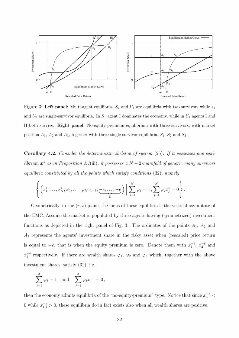
Figure 3: Left panel: Multi-agent equilibria. S2 and U1 are equilibria with two survivors while s1

and U2 are single-survivor equilibria. In S1 agent I dominates the economy, while in U1 agents I and

II both survive. Right panel: No-equity-premium equilibrium with three survivors, with market

position A1, A2 and A3, together with three single survivor equilibria, S1, S2 and S3.

Corollary 4.2. Consider the deterministic skeleton of system (25). If it possesses one equi-

librium x∗ as in Proposition 4.1(iii), it possesses a N − 2-manifold of generic many survivors

equilibria constituted by all the points which satisfy conditions (32), namely

(x∗1, . . . , x

∗N ; ϕ1, . . . , ϕN−1−k;−e, . . . ,−e︸︷︷︸

L

) ∣∣∣∣N∑

j=1

ϕj = 1 ,

N∑j=1

ϕjx∗j = 0

.

Geometrically, in the (r, x) plane, the locus of these equilibria is the vertical asymptote of

the EMC. Assume the market is populated by three agents having (symmetrized) investment

functions as depicted in the right panel of Fig. 3. The ordinates of the points A1, A2 and

A3 represents the agents’ investment share in the risky asset when (rescaled) price return

is equal to −e, that is when the equity premium is zero. Denote them with x−e1 , x−e

2 and

x−e3 respectively. If there are wealth shares ϕ1, ϕ2 and ϕ3 which, together with the above

investment shares, satisfy (32), i.e.

3∑j=1

ϕj = 1 and3∑

j=1

ϕjx−e1 = 0 ,

then the economy admits equilibria of the “no-equity-premium” type. Notice that since x−e3 <

0 while x−e1,2 > 0, these equilibria do in fact exists also when all wealth shares are positive.

32

4.3 Stability of multi-agents equilibria

This Section presents the stability analysis of the equilibria defined in Proposition 4.1. The

three Propositions below provide the stability region in the parameter space for the cases

enumerated in Proposition 4.1, i.e. for the generic case of a single survivor, for the non-

generic case of many survivors and for the generic case with many survivors and without

equity premium. The derivation of these Propositions requires quite cumbersome algebraic

manipulations and we refer the reader to Appendix G for the intermediate lemmas and final

proofs.

For the generic case of a single survivor equilibrium we have the following

Proposition 4.2. Let x∗ be a fixed point of (25) associated with a single survivor PCE.

Without loss of generality we can assume that the survivor is the first agent. Let Pf1(µ)

denote the (L − 1)-dimensional stability polynomial associated with the investment function

of the survivor. The equilibrium x∗ is (locally) asymptotically stable if the two following

conditions are met:

1) all roots of the polynomial

Q1(µ) = µL+1 − (1 + r∗) µ− 1

r∗ l′(r∗)Pf1(µ) , (33)

are inside the unit circle.

2) the equilibrium investment shares of the non-surviving agents satisfy

−2− r∗ < x∗n(r∗ + e

)< r∗ , 1 < n ≤ N . (34)

The equilibrium x∗ is unstable if at least one of the roots of the polynomial in (33) is outside

the unit circle or if at least one of the inequalities in (34) holds with the opposite (strict) sign.

In particular, the system exhibits a fold bifurcation if one of the N−1 right-hand inequalities

in (34) becomes an equality and a flip bifurcation if one of the N − 1 left-hand inequalities

becomes an equality.

33

Inve

stm

ent S

hare



0

1

-1 -e- 0

S1

U1

S2

U2

E

I II

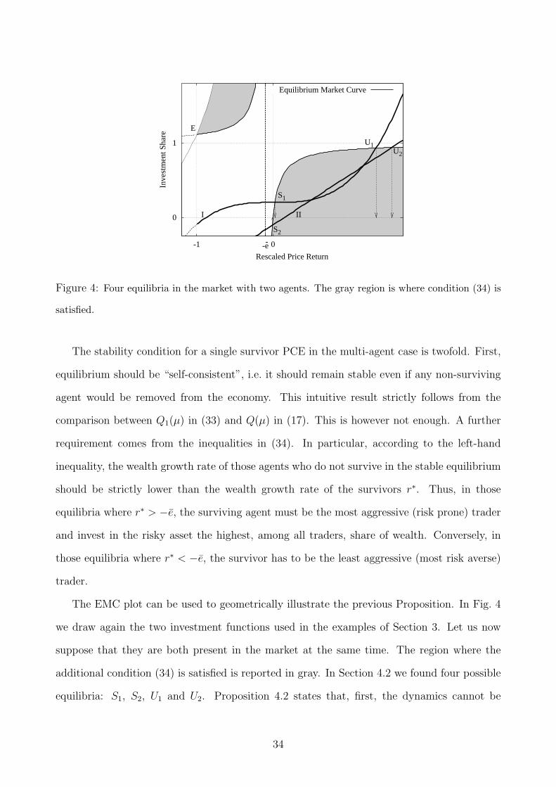
Figure 4: Four equilibria in the market with two agents. The gray region is where condition (34) is

satisfied.

The stability condition for a single survivor PCE in the multi-agent case is twofold. First,

equilibrium should be “self-consistent”, i.e. it should remain stable even if any non-surviving

agent would be removed from the economy. This intuitive result strictly follows from the

comparison between Q1(µ) in (33) and Q(µ) in (17). This is however not enough. A further

requirement comes from the inequalities in (34). In particular, according to the left-hand

inequality, the wealth growth rate of those agents who do not survive in the stable equilibrium

should be strictly lower than the wealth growth rate of the survivors r∗. Thus, in those

equilibria where r∗ > −e, the surviving agent must be the most aggressive (risk prone) trader

and invest in the risky asset the highest, among all traders, share of wealth. Conversely, in

those equilibria where r∗ < −e, the survivor has to be the least aggressive (most risk averse)

trader.

The EMC plot can be used to geometrically illustrate the previous Proposition. In Fig. 4

we draw again the two investment functions used in the examples of Section 3. Let us now

suppose that they are both present in the market at the same time. The region where the

additional condition (34) is satisfied is reported in gray. In Section 4.2 we found four possible

equilibria: S1, S2, U1 and U2. Proposition 4.2 states that, first, the dynamics cannot be

34

attracted by an equilibrium which was unstable in the respective single-agent case. And,

second, it cannot be attracted by an equilibrium in which non-surviving agents investment

shares at equilibrium belong to the white region. As we have seen in Section 4.2, if an

agent uses EWMA or CWA forecast the points U1 and U2 will be unstable (cf. examples 2

and 3 in Section 3.3). Therefore, they will be unstable also in the multi-agents case. From

item 2) of Proposition 4.2 it follows that S1 is the only stable equilibrium of the two agents

system. Notice, indeed, that in the abscissa of S1, i.e. for the equilibrium return, the linear

investment function of the non-surviving agent II passes below the investment function of the

surviving agent and belongs to the gray area. On the contrary, in the abscissa of S2, the

investment function of the non-surviving agent I is higher and does not belong to the gray

area. Consequently, this equilibrium is unstable. A similar situation occurs in the right panel

of Fig. 3. Among the three single survivor equilibria S1, S2 and S3, only the first is stable.

Let us move now to consider the non-generic case, when k different agents survive in the

equilibrium. The following applies

Proposition 4.3. Let x∗ be a fixed point of (25) associated with a k survivors PCE, as defined

by (28), (30) and (31).

The fixed point x∗ is never hyperbolic and, consequently, never (locally) asymptotically sta-

ble. Its non-hyperbolic submanifold is the k−1-dimensional manifold defined in Corollary 4.1.

Let Pfn(µ) be the stability polynomial associated with the investment function fn. The

equilibrium x∗ is (locally) stable if the two following conditions are met:

1) all the roots of the polynomial

Q1¦k(µ) = µL+1 − (1 + r∗) µ− 1

r∗ l′(r∗)

k∑n=1

ϕ∗n Pfn(µ) , (35)

are inside the unit circle.

2) the equilibrium investment shares of the non-surviving agents satisfy

−2− r∗ < x∗n (r∗ + e) < r∗ , k < n ≤ N . (36)

35

The equilibrium x∗ is unstable if at least one of the roots of the polynomial in (35) is outside

the unit circle or if at least one of the inequalities in (36) holds with the opposite (strict) sign.

The non-hyperbolic nature of the equilibria with many survivors turns out to be a direct

consequence of their non-unique specifications. The motion of the system along the k − 1

dimensional subspace consisting of the continuum of equilibria defined in Corollary 4.1 leaves

the aggregate properties of the system invariant so that all these equilibria can be considered

equivalent. Proposition 4.3 also provides the stability conditions for perturbations in the

hyperplane orthogonal to the non-hyperbolic manifold formed by equivalent equilibria. The

polynomial Q1¦k(µ) is quite similar to the corresponding polynomial in Proposition 4.2, except

that one has to weight the stability polynomial of the different investment functions Pfk(µ)

with the weights corresponding to the relative wealth of survivors. At the same time, the

constraint on the investment shares (36) is identical to the one obtained in (34). Similarly to

the case with a single survivor, in those equilibria where r∗ > −e all surviving agents must

be more aggressive buyer of risky asset than those who do not survive, and vice versa for

r∗ < −e.

Finally, let us analyze the generic many survivors equilibria with r∗ = −e. Without loss

of generality, we assume that the survivors are the first k ≤ N agents. The following result

characterizes the stability of such equilibria

Proposition 4.4. Let x∗ be a fixed point of system (25) belonging to a N − 2-dimensional

manifold of k-survivors equilibria defined by (28) and (32).

If N ≥ 3, the fixed point x∗ is non-hyperbolic and, consequently, is not (locally) asymptot-

ically stable. The equilibrium x∗ is (locally) stable if all the roots of the following polynomial

are inside the unit circle

µL+1 +µ− 1⟨

x2⟩

k∑j=1

ϕ∗j Pfj(µ) , (37)

where Pfj(µ) is the stability polynomial of the investment function fj computed in (−e, . . . ,−e),

and⟨x2

⟩=

∑kn=1 ϕ∗n x∗n

2.

36

Inve

stm

ent S

hare



0

-e- 0

SL

U

SH

Inve

stm

ent S

hare



0

-e- 0

SL

U

SH

SM

Figure 5: Left Panel: Non-linear investment function leading to multiple equilibria. SH and SL are

stable while U is unstable. A second linear investment function always lays below the first. Right

Panel: The linear investment function is raised above SL. As a result, market now possesses a new

stable equilibria, SM , while SL looses its stability. In the stable equilibria SH and SM two different

agents survive.

The equilibrium x∗ is unstable if at least one of the roots of polynomial in (37) is outside

the unit circle.

As in the case of Proposition 4.3, the “no-equity-premium” equilibria can be non-hyperbolic,

due to the possibility to reallocate wealth between agents without affecting the aggregate prop-

erties of the dynamics. Once the functional form of the investment functions is known, one can

derive the expression of the polynomial Q and obtain the appropriate stability conditions from

the analysis of its roots, analogously to what has been done in the examples of Section 3.3. In

particular, when all the investment functions possess a zero slope in −e, the equilibria (if they

exist) are always stable. Consider the right panel of Fig. 3. Since the investment functions

of agent I and II are flat in A1 and A2 respectively, if the wealth share of agent III is small

enough, then the no-equity-premium equilibrium is stable.

4.4 Optimal selection and multiple stable equilibria

In this Section, using the geometric interpretation based on the EMC, we discuss the implica-

tions of Proposition 4.2 about the asymptotic behavior of the model and its global properties.

37

For definiteness, we will mainly confine the discussion to the generic case of equilibria with a

single survivor, but many aspects of it do apply in general.

The first implication concerns the aggregate dynamics of the economy. Let us consider

a stable many-agent equilibrium x∗. Let us suppose that r∗ is the equilibrium return in x∗

and that the first agent survives. Then his wealth return is equal to r∗ and this is also the

asymptotic growth rate of the total wealth. Then, we can interpret the second requirement

of Proposition 4.2 as saying that, in the dynamic resulting from the competition of different

trading strategies, the surviving agent is the one who allows the economy to have the highest

possible rate of growth. Indeed, if any other agent n 6= 1 survived, the economy would have

grown at a rate x∗n (r∗ + e), which is lower than r∗ according to (34). This result constitutes

a sort of optimal selection principle since it clearly states the market endogenous selection

toward the best aggregate outcome. Indeed, the market selection mechanism seems to act

in accordance with the asymptotic behavior of the system. In equilibria with r∗ > −e the

aggregate wealth is growing. In this case, and according to the optimal selection principle, the

surviving agent is the most aggressive investor, so as to guarantee the highest possible growth

rate to the whole economy. Conversely, in equilibria with r∗ < −e, when the wealth of the

economy decreases, the survivor is the least aggressive traders, so that the economy shrinks

at the lowest speed.

Notice, however, that this selection criterion does not apply across the whole set of equi-

libria, but only inside the subset formed by equilibria associated with stable fixed points in

the single agent case (c.f. (35)). For instance, with the investment functions shown in Fig. 4,

the dynamics will never end up in U2, even if this is the equilibrium with the highest possible

return. Furthermore, the variety of possible investment functions implies that the optimal

selection principle has a local character. Indeed, due to the “lock-in” effect generated by the

boundedness of attraction domains, it is possible that the market does not select, among all

stable equilibria, the one which provides the highest returns. An illustrative example is pro-

vided by the “step-wise” investment function shown in the left panel of Fig. 5. This function

possesses two stable equilibria, SL and SH . Now suppose that an agent using this function

38

competes on the market with a second agent, more risk averse, who always invest smaller

shares of wealth in the risky asset. For instance assume that the second agent uses the con-

stant investment function shown in the same plot. In this situation, the two equilibria of

the nonlinear function remain stable and the riskier agent will ultimately dominate the mar-

ket. However, initial conditions completely determine which one of the two equilibria will be

eventually selected by the market.

Staring from the situation in the left panel of Fig. 5, imagine to shift the constant function

upward, so as to cross the step-wise function between SL and SH . The resulting situation

is represented in the right panel of Fig. 5. This change of strategy by the second agent will

affect the economy in different ways, depending on what was the prevailing equilibrium before

the shift. If the system was in SH , no effect is observed and the dominant agent remains the

one with the sigmoid investment function. If instead the economy was in SL, this equilibrium

becomes unstable and the system will tend to move away from it. The ensuing dynamic could

ultimately leads to the dominance of the second agent, so that the system ends up in the

equilibrium SM . This simple example shows that the possibility for a strategy to become

(or remain) dominant does not depend exclusively on the strategy itself, but also, and in

an essential way, on the conditions prevailing in the market when the strategy is actually

implemented and on the global behavior of all other strategies. This result does not only

apply to single survivor equilibria. Indeed another possible source of multiple equilibria is

given by the existence of generic many survivors fixed points identified in Proposition 4.1(iii).

For example, in the situation depicted in the right panel of Fig. 3, there is a stable equilibrium

where agent I survives alone (point S1) and a manifold of generic equilibria where all three

agents survive. In the latter case, if the wealth share of agent I is large enough, according

to Proposition 4.4, all these equilibria are stable and, depending on the initial condition, the

market can display both single survivor or many survivors equilibria.

39

5 Conclusion

This paper introduces novel results concerning the characterization and stability of equilibria

in speculative pure exchange economies with heterogeneous CRRA traders. The framework

is relatively general in terms of agents’ behaviors and differs from most of the Heterogeneous

Agents Models in two important respects. First, we analyze the aggregate dynamics and

asymptotic behavior of the market when an arbitrary large number of traders participate to

the trading activity. Second, we do not restrict in any way the procedure used by agents in

order to build their forecast about future prices, nor the way in which agents can use this

forecast to obtain their present asset demand: any smooth investment function mapping the

information set to the present investment choice can be present in the model.

We confine our analysis to those equilibria in which aggregate market dynamics is consistent

with the procedures adopted by agents to form expectations about future price movement. We

derive a complete characterization of Procedurally Consistent Equilibria (PCE) and a descrip-

tion of their stability conditions in terms of few parameters derived from traders investment

strategies. In particular, we show that a simple function, the “Equilibrium Market Curve”,

can be used to obtain a geometric characterization of the location of all possible equilibria.

Furthermore, some results about stability conditions can also be inferred from the same EMC.

We find that, irrespectively of the number of agents operating in the market and of the

structure of their demand functions, only three types of PCE are possible:

1. isolated fixed points, where a single agent asymptotically possesses the entire wealth of

the economy,

2. non-generic equilibria, associated with continuous manifolds of fixed points, where many

agents possess a finite shares of the total wealth,

3. generic equilibria with many survivors, consistent with no-arbitrage pricing.

The notion of PCE allows us to join together the EF and HAMs approaches. Indeed the

stability conditions for the first two types of PCE (see Propositions 4.2 and 4.3) incorporates

40

two parts. The first part shows that the stability of market dynamics depends on agents’

reactions to past prices, as common to HAMs. This result relates to Grandmont (1998)

who puts forward the general theory of individual learning under expectation feedback in

homogeneous environments. The second part highlights the role played by the wealth-driven

selection, and is essentially the requirement of local evolutionary stability common among the

EF models. Notice that this part is not present in the stability conditions of the PCE of the

third type (see Proposition 4.4), where the no-arbitrage condition makes the wealth selection

dynamics irrelevant.

Our general results provide a simple and clear description of the principles governing the

asymptotic market dynamics resulting from the competition of different trading strategies.

The optimizing agents may dominate non-optimizing agents but may also be dominated by

them. In general, the ultimate result of competition between agents depends on the whole

market ecology. As we have shown, the EMC is a handy tool to discuss such phenomena

as absence of equilibrium, presence of multiple equilibria, and also for comparative statics

exercises. From the “geometric” analysis made possible by the EMC (c.f. the stability analysis

in Section 4.3) the following two “impossibility theorems” follow in an obvious way. First,

there exists no “best” strategy, independently of what “best” means exactly, since any possible

market equilibrium can be destabilized by some investment function. Second, it is impossible

to build a dominance order relation inside the space of trading strategies, since two strategies

may generate multiple stable equilibria with different survivors, so that the outcome will

depend on system initial conditions or on noise.

The main advantage of the present model rests in its ability to provide a relatively sim-

ple framework in which the interplay between agents’ decision processes and market forces

can be studied with reasonable generality. In his famous argument in favor of a rational ap-

proach in economics, Friedman (1953) appeals to the evolutionary ideas of natural selection

to justify optimization. Friedman’s argument states that since market forces tend to weed

out non-rational agents, the modeler can assume that the agents behave as if they are max-

imizers. A number of recent studies has shown that Friedman’s argument is not generally

41

valid (e.g. DeLong, Shleifer, Summers, and Waldmann (1990b), Blume and Easley (1992),

Brock and Hommes (1998)). Our results support this view showing that the survivors in the

market are determined not only by their own strategies but also by the complete behavioral

ecology. Alternatively, one can consider the optimizing agents’ behavior as an outcome of

the learning process. In this case, however, due to possible presence of multiple equilibria or

instability, there is no reason to assume a priori that such learning process will converge to

the corresponding fixed point.

The present analysis can be extended in many directions. First of all, one may raise the

question of the robustness of the results with respect to Assumption 1 about constant dividend

yield. Model in Anufriev and Dindo (2009) investigates the case of growing dividend yield

and shows that some results (as presence of equity premium in equilibria and possibility to

represent the equilibria by the EMC) remain essentially the same. Second, in the limits of

our framework, one can wonder about other possible dynamics. For instance, we have shown

that there is a theoretical possibility of not having any equilibrium at all. The dynamics in

this case remain unknown. We also did not investigate the dynamics after bifurcation, which

is the key question in many heterogeneous agent models. Probably numerical methods can

be effectively applied to study these questions and also clarify the role of initial conditions

and the determinants of the relative size of the basins of attraction for multiple equilibria

scenarios. Third, our general CRRA-framework led us, in Proposition 2.1, to write the system

in terms of returns and wealth shares. There are many behavioral specifications which were

not analyzed here and are still consistent with our framework. These specifications range from

the evaluation of the “fundamental” value of the asset, possibly obtained from a private source

of information, to a strategic behavior that tries to keep in consideration the reaction of other

market participants to the revealed individual choices.

APPENDIX

42

A Proof of Proposition 2.1

Plugging the expression for wt+1,n from the second equation in system (4) into the right-hand side of the first

equation of the same system, and assuming that pt > 0 and, consistently with (6), pt 6=∑xt+1,n xt,n wt,n, one

gets

pt+1 =

(1− 1

pt

N∑n=1

xt+1,n xt,n wt,n

)−1 (N∑n=1

xt+1,n wt,n +(et+1 − 1

) N∑n=1

xt+1,n wt,n xt,n

)=

= pt

∑n xt+1,n wt,n + (et+1 − 1)

∑n xt+1,n wt,n xt,n∑

n xt,n wt,n −∑n xt+1,n xt,n wt,n

=

= pt

⟨xt+1

⟩t− ⟨

xt xt+1

⟩t+ et+1

⟨xt xt+1

⟩t⟨

xt⟩t− ⟨

xt xt+1

⟩t

,

where we used the first equation of (4) rewritten for time t to get the second equality. Condition (6) is obtained

imposing pt+1 > 0, and the dynamics of price return in (7) are immediately derived. From the second equation

of (4) it follows that

wt+1,n = wt,n(1 + xt,n (rt+1 + et+1)

) ∀n ∈ {1, . . . , N} , (38)

leading to (8). To obtain the wealth share dynamics, divide both sides of (38) by wt+1 to have

ϕt+1,n =wt,nwt+1

(1 + xt,n (rt+1 + et+1)

)=

=wt,n∑

m wt,m + (rt+1 + et+1)∑m xt,mwt,m

(1 + xt,n (rt+1 + et+1)

)=

=ϕt,n

1 + (rt+1 + et+1)∑m xt,mϕt,m

(1 + xt,n (rt+1 + et+1)

),

where (38) has been used to get the second line and we divided both numerator and denominator by the total

wealth at time t to get the third.

B Example of agents behavior

Suppressing any agent-specific index, we start with the evolution of the agent’s (rescaled) wealth given by (4)

wt+1 = wt + xtwt (rt+1 + et+1) .

The future wealth depends on the total return zt+1 = rt+1 + et+1 at time t, which is unknown . The decision

to invest a fraction of wealth xt yields the portfolio return

ρt+1 = wt+1/wt − 1 = xt (rt+1 + et+1) .

43

Assume that agent’s utility depends on his portfolio return and has a mean-variance expression with a

constant risk aversion coefficient β > 0. The problem

maxxt

{Et−1[ρt+1]− β

2Vt−1[ρt+1]

}(39)

requires that an agent forms expectations Et−1[zt+1] and Vt−1[zt+1] about the first two moments of future total

return on the basis of the information set It−1 available at the beginning of period t. Solving the optimization

problem (39) one gets

x∗t =1β

Et−1[zt+1]Vt−1[zt+1]

. (40)

Referring to Section 2.3 the right hand-side represents a family of choice’ functions

hβ(θ1, θ2) =1β

θ1θ2,

parameterized by the risk aversion coefficient β. These functions depends on two statistics of the future

returns distribution, θ1 = g1(zt+1) = Et−1[zt+1] and θ2 = g2(zt+1) = Vt−1[zt+1]. The behavior of the agent is

ultimately determined by the expectation functions g1 and g2 used to obtain these statistics.

One possible direction, inspired by the HAMs literature, is to distinguish different types of traders based

on stylized behavior. For example, suppose that “fundamentalists” do not take past observations into account,

but expect an exogenous risk premium (i.e., excess return) gF1 ≡ δ and no excess volatility, i.e., gF2 ≡ σ2e , where

σ2e is the variance of the yield process. As a result of substitution of these expectation functions in the choice

function (40), we obtain the investment function of fundamentalists

hFβ =δ

β σ2e

,

which is constant. Conversely, suppose that “chartists” try to learn the level of return from the past observa-

tions, so that gC1 (It−1) = a+ bzt−1, while they still have constant estimation for the variance, gC2 ≡ σ2e . As a

result, we obtain for the chartists the investment function

hCβ =a+ b(rt−1 + et−1)

β σ2e

,

which is a linear function of the previous total return. Within our framework one can study the dynamics of

a market populated by these two types of traders and address such questions as the role of risk-aversion β,

risk premium δ, or extrapolation coefficient b for the equilibrium and stability of the system. The reader is

referred to Anufriev (2008) for a study of these questions in the case of arbitrary linear investment functions.

The choice function (40) with special linear predictors was previously considered in Chiarella and He (2001).

The discussion above represents but a simple example of an agent investment function. Many generalization

are possible and have been explored in the past. Instead of a mean-variance utility the agent could maximize

the expected utility (EU) of future wealth. Several functional specifications are suggested in the literature, most

44

notably the power utility function for which, however, closed form solutions are in general not available. Or

one can replace the expectation operator with more sophisticated alternative, like the maximin criterion or the

minimax-regret criterion discussed in Brock and Manski (2008). Both these criteria will give choice functions

which depend on a small set of statistics which are in turn specified through the definition of appropriate

expectation functions. Concerning the latter, one can adopt a classical Bayesian approach or, more common

in the HAMs literature, use adaptive learning estimators derived from statistical analysis, like moving windows

estimators of central tendency. Different learning rules of different degree of sophistication have been suggested

in the literature. See Colucci and Valori (2006) for an overview. Since all of them can be represented as a

function of past data, they all satisfy to the requirements of our framework. A typical question in the adaptive

learning literature is whether multiple equilibria are possible and whether they can be approached through

the learning mechanism. One can easily study these questions within our framework, see Section 3.4. What is

more, one can do it in the presence of heterogeneous agents’ behavior.

C Proof of Proposition 3.1

Plugging the equilibrium values of the variables in the first equation of (11), one gets x∗ = f(r∗, . . . , r∗).

Now using R(x∗, x∗, e) = e x∗/(1 − x∗) one can invert the second equation to get (14). Item (ii) follows

directly from condition (6) written at equilibrium. Finally, from (8) using the previous relations one has

ρ∗ = x∗(r∗ + e) = l(r∗)(r∗ + e) = r∗.

D Proof of Proposition 3.2

We start with a simple result which will be useful in what follows.

Lemma D.1.∣∣∣∣∣∣∣∣∣∣∣∣∣∣∣∣∣∣∣∣∣∣∣∣

x1 x2 x3 . . . xn−1 xn

1 −µ 0 . . . 0 0

0 1 −µ . . . 0 0

0 0 1 . . . 0 0...

......

. . ....

...

0 0 0 . . . −µ 0

0 0 0 . . . 1 −µ

∣∣∣∣∣∣∣∣∣∣∣∣∣∣∣∣∣∣∣∣∣∣∣∣

= (−1)n+1n∑

k=1

xk µn−k , (41)

Proof. Consider this determinant as a sum of elements from the first row multiplied on the corresponding

minor. The minor of element xk, whose corresponding sign is (−1)k+1, is a block-diagonal matrix consisting of

45

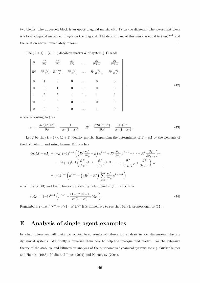
two blocks. The upper-left block is an upper-diagonal matrix with 1’s on the diagonal. The lower-right block

is a lower-diagonal matrix with −µ’s on the diagonal. The determinant of this minor is equal to (−µ)n−k and

the relation above immediately follows.

The (L+ 1)× (L+ 1) Jacobian matrix J of system (11) reads

∥∥∥∥∥∥∥∥∥∥∥∥∥∥∥∥∥∥∥∥∥∥∥∥∥∥

0 ∂f∂r0

∂f∂r1

∂f∂r2

. . . ∂f∂rL−2

∂f∂rL−1

Rx Rf ∂f∂r0 Rf ∂f∂r1 Rf ∂f∂r2 . . . Rf ∂f∂rL−2

Rf ∂f∂rL−1

0 1 0 0 . . . 0 0

0 0 1 0 . . . 0 0...

......

.... . .

......

0 0 0 0 . . . 0 0

0 0 0 0 . . . 1 0

∥∥∥∥∥∥∥∥∥∥∥∥∥∥∥∥∥∥∥∥∥∥∥∥∥∥

, (42)

where according to (12)

Rx =∂R(x∗, x∗)

∂x= − 1

x∗ (1− x∗)Rf =

∂R(x∗, x∗)∂x′

=1 + r∗

x∗ (1− x∗). (43)

Let I be the (L+ 1)× (L+ 1) identity matrix. Expanding the determinant of J − µ I by the elements of

the first column and using Lemma D.1 one has

det(J − µ I

)= (−µ) (−1)L−1

((Rf

∂f

∂r0− µ

)µL−1 +Rf

∂f

∂r1µL−2 + · · ·+Rf

∂f

∂rL−1

)−

−Rx (−1)L−1

(∂f

∂r0µL−1 +

∂f

∂r1µL−2 + · · ·+ ∂f

∂rL−2µ+

∂f

∂rL−1

)=

= (−1)L−1

(µL+1 −

(µRf +Rx

) L−1∑

k=0

∂f

∂rkµL−1−k

),

which, using (43) and the definition of stability polynomial in (16) reduces to

PJ(µ) = (−1)L−1

(µL+1 − (1 + r∗)µ− 1

x∗(1− x∗)Pf (µ)

). (44)

Remembering that l′(r∗) = x∗(1− x∗)/r∗ it is immediate to see that (44) is proportional to (17).

E Analysis of single agent examples

In what follows we will make use of few basic results of bifurcation analysis in low dimensional discrete

dynamical systems. We briefly summarize them here to help the unacquainted reader. For the extensive

theory of the stability and bifurcation analysis of the autonomous dynamical systems see e.g. Guckenheimer

and Holmes (1983), Medio and Lines (2001) and Kuznetsov (2004).

46

A fixed point of a discrete dynamical system is asymptotically stable if all the eigenvalues of the Jacobian

matrix computed in the fixed point are inside the complex unit circle. For two-dimensional dynamical systems

this amount to

Proposition E.1 (Sufficient conditions for the local stability). The fixed point of a two-dimensional discrete

dynamical system is locally asymptotically stable if the following conditions are satisfied

d < 1 , t < 1 + d , t > −1− d . (45)

where t and d are, respectively, the trace and the determinant of the Jacobian matrix computed in the fixed

point.

The fixed point is unstable if at least one of the eigenvalues lies outside the unit circle. The situation

in which the change of one or more parameters of the system leads to the cross of the unit circle by one (or

two complex conjugated) eigenvalues is called a bifurcation. Three types of generic bifurcations are usually

considered, depending on where the unit circle is crossed. A bifurcation is called fold, flip or Neimark-Sacker,

if an eigenvalues crosses the unit circle in 1, −1 or outside the real axis, respectively.For two-dimensional

dynamical system this amount to

Proposition E.2. The fixed point of a two-dimensional discrete dynamical system looses its stability when one

of the inequalities in conditions (45) is changing its sign. The system exhibits a Neimark-Sacker bifurcation if

d = 1, a fold bifurcation if t = 1 + d, and a flip bifurcation if t = −1− d.

E.1 Stability for the system with short memory forecast

In this case the second degree polynomial associated with the constant stability polynomial reads

Q(µ) = µ2 − f ′(r∗)l′(r∗) r∗

((1 + r∗

)µ− 1

),

and Proposition 3.3 follows straight-forwardly from the application of the two Propositions above.

E.2 Stability for the system with Constant Weighted forecast

The characteristic polynomial for this case can be written as follows:

Q(µ) = µL−1

(µ2 − 1

L

1− (1/µ)L

1− 1/µY

X

((1 +X)µ− 1

)), (46)

where, as before, variables X = r∗ and Y = f ′(r∗)/l′(r∗) correspond to the abscissa and ordinate of the

stability region diagrams in Fig. 2.

47

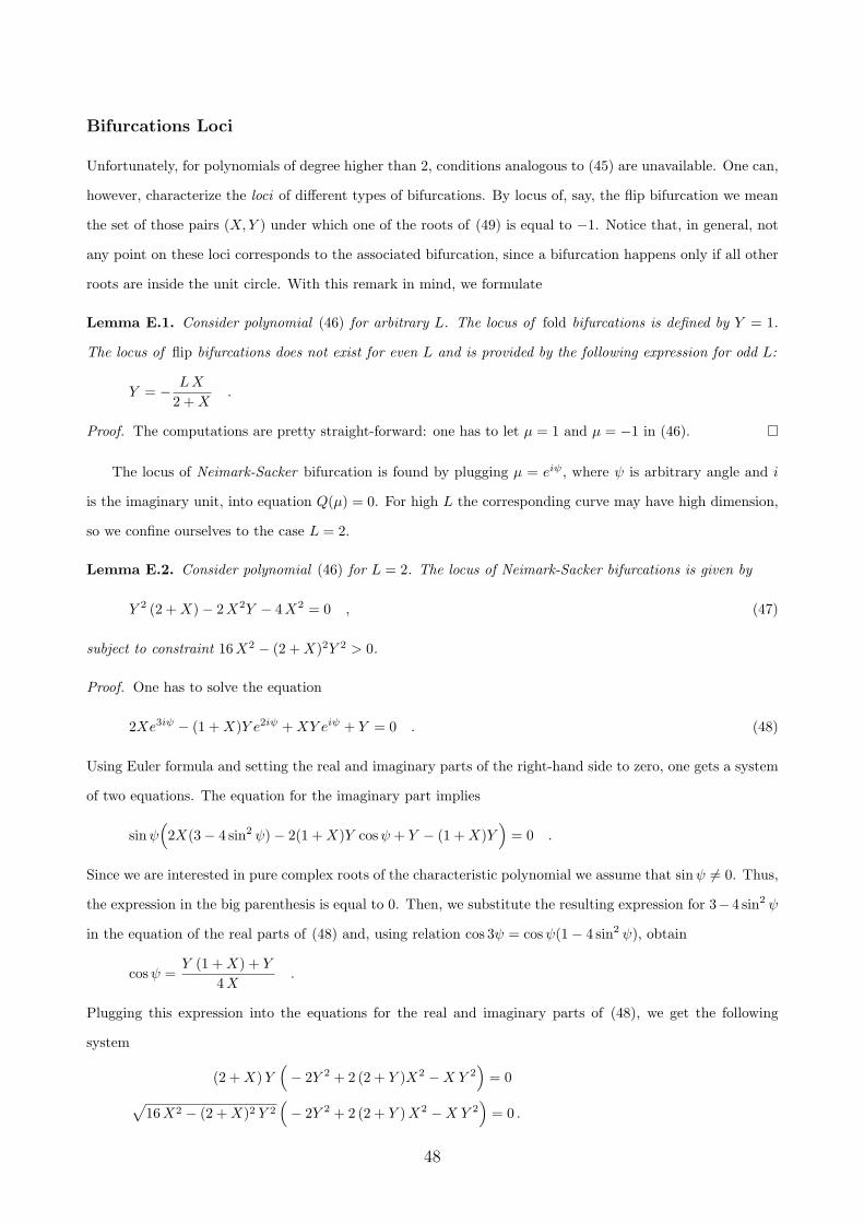
Bifurcations Loci

Unfortunately, for polynomials of degree higher than 2, conditions analogous to (45) are unavailable. One can,

however, characterize the loci of different types of bifurcations. By locus of, say, the flip bifurcation we mean

the set of those pairs (X,Y ) under which one of the roots of (49) is equal to −1. Notice that, in general, not

any point on these loci corresponds to the associated bifurcation, since a bifurcation happens only if all other

roots are inside the unit circle. With this remark in mind, we formulate

Lemma E.1. Consider polynomial (46) for arbitrary L. The locus of fold bifurcations is defined by Y = 1.

The locus of flip bifurcations does not exist for even L and is provided by the following expression for odd L:

Y = − LX

2 +X.

Proof. The computations are pretty straight-forward: one has to let µ = 1 and µ = −1 in (46).

The locus of Neimark-Sacker bifurcation is found by plugging µ = eiψ, where ψ is arbitrary angle and i

is the imaginary unit, into equation Q(µ) = 0. For high L the corresponding curve may have high dimension,

so we confine ourselves to the case L = 2.

Lemma E.2. Consider polynomial (46) for L = 2. The locus of Neimark-Sacker bifurcations is given by

Y 2 (2 +X)− 2X2Y − 4X2 = 0 , (47)

subject to constraint 16X2 − (2 +X)2Y 2 > 0.

Proof. One has to solve the equation

2Xe3iψ − (1 +X)Y e2iψ +XY eiψ + Y = 0 . (48)

Using Euler formula and setting the real and imaginary parts of the right-hand side to zero, one gets a system

of two equations. The equation for the imaginary part implies

sinψ(2X(3− 4 sin2 ψ)− 2(1 +X)Y cosψ + Y − (1 +X)Y

)= 0 .

Since we are interested in pure complex roots of the characteristic polynomial we assume that sinψ 6= 0. Thus,

the expression in the big parenthesis is equal to 0. Then, we substitute the resulting expression for 3−4 sin2 ψ

in the equation of the real parts of (48) and, using relation cos 3ψ = cosψ(1− 4 sin2 ψ), obtain

cosψ =Y (1 +X) + Y

4X.

Plugging this expression into the equations for the real and imaginary parts of (48), we get the following

system

(2 +X)Y(− 2Y 2 + 2 (2 + Y )X2 −X Y 2

)= 0

√16X2 − (2 +X)2 Y 2

(− 2Y 2 + 2 (2 + Y )X2 −X Y 2

)= 0 .

48

In any solution of this system, the common expression in the parenthesis must be equal to zero, which gives

(47). Additional constraint guarantees that the squared root in the second equation is real.

In the upper right panel of Fig. 2 the curve (47) is reported together with the loci derived in Lemma E.1.

Limiting case, L →∞

The behavior of the locus of flip bifurcations when the memory parameter increases may suggest that any

point of the system for which f ′/l′ < 1 can be stabilized for large enough value of L. Indeed, let us consider

the region outside of the unit circle (including the circle itself), fix µ = µ0 and let L→∞. Since |µ0| ≥ 1, it

is 1/µL0 → 0 and (46) reduces to

µL0µ0 − 1

(µ2

0 − µ0(1 + o(1L

))

which does not admit zeros outside the unit circle irrespectively of the value of X and Y .

E.3 Stability for the system with EWMA forecast

Using stability polynomial (22), the characteristic polynomial for this case can be written as follows:

Q(µ) = µL−1

(µ2 − 1− λ

1− λL1− (λ/µ)L

1− λ/µ

Y

X

((1 +X)µ− 1

)), (49)

where X = r∗ and Y = f ′(r∗)/l′(r∗). We proceed through the same steps as in the previous case.

Bifurcations Loci

First we characterize the loci of fold and flip bifurcations.

Lemma E.3. Consider polynomial (49) for arbitrary λ and L. The locus of fold bifurcations is given by

Y = 1, while the locus of flip bifurcations is provided as follows:

1 + Y2 +X

X

1− λ

1 + λ

1 + λL

1− λL= 0 for L odd and 1 + Y

2 +X

X

1− λ

1 + λ= 0 for L even .

Proof. The direct substitution of µ = 1 and µ = −1 to (49) leads to the conclusion.

For the locus of Neimark-Sacker bifurcations we consider the case L = 2 and prove the following

Lemma E.4. Consider polynomial (49) for L = 2 and arbitrary λ. The locus of Neimark-Sacker bifurcations

is given by the following curve of the second order

Y 2 λ(X + 1 + λ

)+ Y X (1 + λ)

(1− λ− λX

)−X2 (1 + λ)2 = 0 , (50)

subject to constraint 4(1 + λ2)X2 − (1 + λ+X)2Y 2 > 0.

49

Proof. The proof is completely analogous to that of Lemma E.2.

The curve (50) is depicted in the lower left panel of Fig. 2 together with the loci derived in Lemma E.3.

The construction of the stability region is completed applying the property of continuity of the roots of a

polynomial on its coefficients.

Limiting case, L →∞

Finally, we sketch here a heuristic proof of Proposition 3.4 Consider a value µ0 outside the unit circle, |µ0| ≥ 1.

When L→∞, since λ < 1, it is (λ/µ0)L → 0 so that (49) reduces to

µL−10

1− λ/µ0

(µ2

0 − λµ0 − (1− λ)Y

X((1 +X)µ0 − 1) = 0

).

Since |µ0| > λ for any value of λ, the fraction is finite and bounded away from zero. By applying the conditions

in Proposition E.1 to the last equation one sees that if (23) are satisfied, its roots are inside the unit circle.

F Proof of Proposition 4.1

¿From block X one immediately has (28). From the first row of block R it is

r∗ = e

∑N−1n=1 ϕ

∗nx∗n

2 +(1−∑N−1

n=1 ϕ∗n

)x∗N

2

∑N−1n=1 ϕ

∗n x

∗n (1− x∗n) +

(1−∑N−1

n=1 ϕ∗n

)x∗N (1− x∗N )

. (51)

Let us, first, assume that r∗ + e 6= 0. Then, from block W using (27) one obtains

ϕ∗n = 0 or∑N−1

m=1ϕ∗m x

∗m +

(1−

∑N−1

m=1ϕ∗m

)x∗N = x∗n ∀n ∈ {1, . . . , N − 1} . (52)

Together with (51) this equation admits two types of solutions, depending on whether one or many equilibrium

wealth shares are different from zero.

If only one wealth share is zero, one can assume ϕ∗1 = 1. In this case (52) is satisfied for all agents. From

(51) one has x∗1 = r∗/(e+ r∗) which together with (28) leads to (29).

If, instead, many agents survive one can assume (30). In this case, the second equality of (52) must be

satisfied for any n ≤ k. Since its left-hand side does not depend on n, a x∗1¦k must exist such that x∗1 = · · · =x∗k = x∗1¦k. Substituting ϕ∗n = 0 for n > k and x∗n = x∗1¦k for n ≤ k in (51) one gets x∗1¦k = r∗/(e + r∗). The

equilibrium return r∗ is implicitly defined combining this last relation with (28) for n ≤ k.

Consider finally the case when r∗+ e = 0. Then all equations in block W are satisfied, while (51) straight-

forwardly leads to (32).

The equilibrium wealth growth rates of the survivors are immediately obtained from (8) and (28).

50

G Proofs of Propositions of Section 4.3

Before proving Propositions 4.2, 4.3 and 4.4 we need some preliminary results. The Jacobian matrix of the

deterministic skeleton of system (25) is a(2N + L − 1

) × (2N + L − 1

)matrix. Using the block structure

introduced in Section 4.1 it is separated in 9 blocks

J =

∥∥∥∥∥∥∥∥∥∥∥∥

∂X∂X

∂X∂W

∂X∂R

∂W∂X

∂W∂W

∂W∂R

∂R∂X

∂R∂W

∂R∂R

∥∥∥∥∥∥∥∥∥∥∥∥

, (53)

The block ∂X/∂X is a N×N matrix containing the partial derivatives of the agents’ present investment choices

with respect to the agents’ past investment choices. According to (10) the investment choice of any agent does

not explicitly depend on the investment choices in the previous period, therefore[∂X

∂X

]

n,m

=∂fn∂xm

= 0 , 1 ≤ n,m ≤ N ,

and this block is a zero matrix.

The block ∂X/∂W is a N × (N − 1) matrix containing the partial derivatives of the agents’ investment

choices with respect to the agents’ wealth shares. According to (10) this is a zero matrix and[∂X

∂W

]

n,m

=∂fn∂ϕm

= 0 , 1 ≤ n ≤ N , 1 ≤ m ≤ N − 1 .

The block ∂X/∂R is a N × L matrix containing the partial derivatives of the agents’ investment choices

with respect to the past returns. We use the following notation[∂X

∂R

]

n,l

=∂fn∂rl−1

= frl−1n , 1 ≤ n ≤ N , 1 ≤ l ≤ L .

The definitions of the other blocks will make use of the functions R and Φn which have been defined in

(26) and (27), respectively. Function R depends on agents’ contemporaneous investment choices given by the

investment functions fm, on agents’ previous investment choices xt,m and on agents’ wealth shares ϕt,m. Let

denote the corresponding derivatives as Rfm , Rxm and Rϕm . The function Φn depends on agents’ previous

investment choices xt,m, on agents’ wealth shares ϕt,m and on the value of return given by function R. The

corresponding derivatives are denoted as Φxmn , Φϕm

n and ΦRn .

The block ∂W/∂X is a (N − 1)×N matrix containing the partial derivatives of the agents’ wealth shares

with respect to the agents’ investment choices. It is[∂W

∂X

]

n,m

=∂ϕn∂xm

= Φxmn + ΦRn ·Rxm , 1 ≤ n ≤ N − 1 , 1 ≤ m ≤ N . (54)

The block ∂W/∂W is a (N − 1)× (N − 1) matrix containing the partial derivatives of the agents’ wealth

shares with respect to the agents’ wealth shares. It is[∂W

∂W

]

n,m

=∂ϕn∂ϕm

= Φϕmn + ΦRn ·Rϕm , 1 ≤ n,m ≤ N − 1 . (55)

51

The block ∂W/∂R is a (N − 1) × L matrix containing the partial derivatives of the agents’ wealth share

with respect to lagged returns. It reads

[∂W

∂R

]

n,l

=∂ϕn∂rl−1

= ΦRn ·N∑m=1

Rfmfrl−1m , 1 ≤ n ≤ N − 1 , 1 ≤ l ≤ L . (56)

The block ∂R/∂X is the L×N matrix containing the partial derivatives of the lagged returns with respect

to the agents’ investment choices. Its structure is simple, since only the first line can contain non-zero elements.

It reads

[∂R

∂X

]

l,n

=

Rxn l = 1

0 otherwise, 1 ≤ l ≤ L , 1 ≤ n ≤ N .

The block ∂R/∂W is the L× (N − 1) matrix containing the partial derivatives of the lagged returns with

respect to agents’ wealth shares. It also has L− 1 zero rows and reads

[∂R

∂W

]

l,n

=

Rϕn l = 1

0 otherwise, 1 ≤ l ≤ L , 1 ≤ n ≤ N − 1 .

The block ∂R/∂R is the L×L matrix containing the partial derivatives of the lagged returns with respect

to themselves.

[∂R

∂R

]=

∥∥∥∥∥∥∥∥∥∥∥∥∥∥∥∥∥

Rr0 Rr1 . . . RrL−2 RrL−1

1 0 . . . 0 0

0 1 . . . 0 0...

.... . .

......

0 0 . . . 1 0

∥∥∥∥∥∥∥∥∥∥∥∥∥∥∥∥∥

,

where Rrl =∑Nm=1R

fmfrlm .

With the previous definitions and differentiating the correspondent functions, one obtains

Lemma G.1. Let x∗ be an equilibrium of system (25). The corresponding Jacobian matrix, J(x∗), has the

following structure, where the actual values of non-zero elements vary depending on whether there exists an

52

equity premium in x∗.∥∥∥∥∥∥∥∥∥∥∥∥∥∥∥∥∥∥∥∥∥∥∥∥∥∥∥∥∥∥∥∥∥∥∥∥∥∥∥∥∥∥∥∥∥∥

0 . . . 0 0 . . . 0 0 . . . 0 0 . . . 0 fr01 . . . frL−21 f

rL−11

.... . .

......

. . ....

.... . .

......

. . ....

.... . .

......

0 . . . 0 0 . . . 0 0 . . . 0 0 . . . 0 fr0N . . . frL−2N f

rL−1N

? . . . ? 0 . . . 0 ? . . . ? ? . . . ? ? . . . ? ¥

[ Φx ]...

. . .... [ Φϕ1,k ] [ Φϕk+1,N ] [ Φr ]

...

? . . . ? 0 . . . 0 ? . . . ? ? . . . ? ? . . . ? ¥

0 . . . 0 0 . . . 0 0 . . . 0 F . . . 0 0 . . . 0 0...

. . ....

.... . .

......

. . ....

.... . .

......

. . ....

...

0 . . . 0 0 . . . 0 0 . . . 0 0 . . . F 0 . . . 0 0

Rx1 . . . Rxk 0 . . . 0 Rϕ1 . . . Rϕk Rϕk+1 . . . RϕN−1 Rr0 . . . RrL−2 RrL−1

0 . . . 0 0 . . . 0 0 . . . 0 0 . . . 0 1 . . . 0 0...

. . ....

.... . .

......

. . ....

.... . .

......

. . ....

...

0 . . . 0 0 . . . 0 0 . . . 0 0 . . . 0 0 . . . 1 0

∥∥∥∥∥∥∥∥∥∥∥∥∥∥∥∥∥∥∥∥∥∥∥∥∥∥∥∥∥∥∥∥∥∥∥∥∥∥∥∥∥∥∥∥∥∥

Namely, the “varying” elements belong to the 4 blocks filled by ?’s and denoted as [Φx], [Φϕ1,k], [Φϕk+1,N ] and

[Φr]. In particular, all the elements of the latter block are zeros in the equilibrium with equity premium.

Furthermore, in such equilibrium the elements labeled as ¥’s are also 0’s. Finally, the elements labeled as F’s

on the diagonal of the central block are all equal to 1 in the no-equity-premium equilibria.

Proof. For the computation of the elements in the second big row-block, it will be useful to establish the values

of relevant derivatives in equilibrium. In general it is

Φxmn = ϕ∗n

(δn,m − ϕ∗m)(r∗ + e)1 + (r∗ + e)

⟨x∗

⟩ , Rxm = ϕ∗mx∗m(r∗ + e)− 1− r∗⟨

x∗(1− x∗)⟩ ,

ΦRn = ϕ∗nx∗n −

⟨x∗

⟩

1 + (r∗ + e)⟨x∗

⟩ , Rfm = ϕ∗m1 + x∗m(r∗ + e)⟨x∗(1− x∗)

⟩ ,

Φϕmn =

δn,m(1 + x∗n(r∗ + e)

)− ϕ∗n(r∗ + e)(x∗m − x∗N )1 + (r∗ + e)

⟨x∗

⟩ ,

Rϕm =(e+ r∗)(x∗

2

m − x∗2

N )− r∗(x∗m − x∗N )⟨x∗(1− x∗)

⟩ .

Consider the equilibrium with r∗ 6= −e, i.e. the one described in Proposition 4.1(i) and (ii). Since in such an

equilibrium all survivors invest the same wealth share in the risky asset, one has ΦRn = 0 for any agent n, so

53

that

[∂W

∂X

]

n,m

=

/m, n ≤ k/ = ϕ∗n(δn,m − ϕ∗m

)(e+ r∗)/(1 + r∗)

/otherwise/ = 0

[∂W

∂W

]

n,m

=

/n > k , n 6= m/ = 0

/otherwise/ =(δn,m

(1 + x∗n(r∗ + e)

)− ϕ∗n(r∗ + e)(x∗m − x∗N ))/

(1 + r∗)[∂W

∂R

]

n,m

= 0 , ∀n,m .

(57)

On the other hand, in an equilibrium with r∗ = −e, i.e. the one described in Proposition 4.1(iii), it is Φxmn = 0,

Φϕmn = δn,m and ΦRn = ϕ∗nx

∗n for all possible n and m. Thus, one has

[∂W

∂X

]

n,m

=

/for m,n ≤ k/ = (1− e)ϕ∗n ϕ∗m x

∗n

/⟨x2

⟩

/otherwise/ = 0;

[∂W

∂W

]

n,m

=

/for n ≤ k/ = δn,m − e ϕ∗n x∗n(x∗m − x∗N )/

⟨x2

⟩

/otherwise/ = δn,m

;

[∂W

∂R

]

n,m

=

/for n ≤ k/ = −ϕ∗nx∗n∑Nm=1 ϕ

∗mf

rl−1m

/⟨x2

⟩

/otherwise/ = 0.

(58)

Lemma G.2. Consider equilibrium x∗ with r∗ 6= −e. The characteristic polynomial PJ of the matrix J(x∗)

reads

PJ(µ) = (−1)N+L µN−1 (1− µ)k−1N∏

j=k+1

(1 + x∗j (r∗ + e)

1 + r∗− µ

)

µL+1 − (1 + r∗)µ− 1

x∗1¦k(1− x∗1¦k)

k∑

j=1

ϕ∗j Pfj (µ)

(59)

where Pfn is the stability polynomial associated to the n-th investment function as defined in (16).

Proof. The following proof is constructive: we will identify in succession the factors appearing in (59). At each

step, a set of eigenvalues is found and the problem is reduced to the analysis of the residual matrix obtained

removing the rows and columns associated with the relative eigenspace.

Consider the Jacobian matrix in Lemma G.1. The last N − k columns of the left blocks contain only zero

entries so that the matrix possesses eigenvalue 0 with (at least) multiplicity N − k. Moreover, in each of the

last N − 1− k rows in the central blocks the only non-zero entries belong to the main diagonal. Consequently,

Φϕj

j for k + 1 ≤ j ≤ N − 1 are eigenvalues of the matrix, with multiplicity (at least) one. A first contribution

54

to the characteristic polynomial is then determined as

(−µ)N−kN−1∏

j=k+1

(Φϕj

j − µ) = (−µ)N−kN−1∏

j=k+1

(1 + x∗j (r

∗ + e)1 + r∗

− µ

)(60)

where we used (57) to compute Φϕj

j at equilibrium.

In order to find the remaining part of the characteristic polynomial we eliminate the rows and columns

associated to the previous eigenvalues to obtain

L =

∥∥∥∥∥∥∥∥∥∥∥∥∥∥∥∥∥∥∥∥∥∥∥∥∥∥∥∥∥∥∥∥∥∥∥∥∥∥∥

0 . . . 0 0 . . . 0 fr01 . . . frL−21 f

rL−11

.... . .

......

. . ....

.... . .

......

0 . . . 0 0 . . . 0 fr0k . . . frL−2k f

rL−1k

Φx11 . . . Φxk

1 Φϕ11 . . . Φϕk

1 0 . . . 0 0...

. . ....

.... . .

......

. . ....

...

Φx1k . . . Φxk

k Φϕ1k . . . Φϕk

k 0 . . . 0 0

Rx1 . . . Rxk Rϕ1 . . . Rϕk Rr0 . . . RrL−2 RrL−1

0 . . . 0 0 . . . 0 1 . . . 0 0...

. . ....

.... . .

......

. . ....

...

0 . . . 0 0 . . . 0 0 . . . 1 0

∥∥∥∥∥∥∥∥∥∥∥∥∥∥∥∥∥∥∥∥∥∥∥∥∥∥∥∥∥∥∥∥∥∥∥∥∥∥∥

(61)

This quadratic matrix has 2k + L rows when k < N . If k = N , representation (61) is, strictly speaking, not

correct. Indeed, there exist only N − 1 wealth shares ϕ’s in the original system, therefore the central block of

the matrix has maximal dimension (N−1)×(N−1). Therefore, in this case, the correct matrix has dimension

(2N + L − 1) × (2N + L − 1) and can be obtained from (61) through the removal of the last row and the

last column in the central blocks. In computing the characteristic polynomial we consider separately the case

when k < N and when k = N .

If k < N from (57) it follows that for n,m ≤ k it is

Φϕmn =

1− ϕ∗n v if n = m

−ϕ∗n v otherwise, where v =

(x∗1¦k − x∗N

) e+ r∗

1 + r∗. (62)

Moreover, since all survivors invest the same share x1¦k, it follows that for m ≤ k

Rϕm = v b , where b = x∗N1 + r∗

x∗1¦k (1− x∗1¦k). (63)

The central column block of the determinant can be represented as∥∥ v b + b1 | . . . | v b + bk

∥∥, where the

55

following column vectors have been introduced

b =∥∥∥ 0 . . . 0

∣∣ −ϕ∗1 . . . −ϕ∗k∣∣ b 0 . . . 0

∥∥∥ ,

b1 =∥∥∥ 0 . . . 0

∣∣ 1− µ . . . 0∣∣ 0 0 . . . 0

∥∥∥ ,

...

bk =∥∥∥ 0 . . . 0

∣∣ 0 . . . 1− µ∣∣ 0 0 . . . 0

∥∥∥ .

We consider each of the columns in the central block as a sum of two terms and, applying the multilinear

property of the determinant, end up with a sum of 2k determinants. Many of them are zeros, since they contain

two or more columns proportional to vector b. There are only k + 1 non-zero elements in the expansion. One

of them has the following structure of the central column block:∥∥ b1 | . . . . . . . . . | bk

∥∥, while k others

possess similar structure in the central column block, with column v b on the ν’th place instead of bν , i.e. for

all ν ∈ {1, . . . , k} the blocks look like∥∥ b1 | . . . | v b | . . . | bk

∥∥.

The central matrix in the one obtained from the former block is diagonal and, therefore, its determinant

is equal to (1− µ)k det M(k), where

M(k) =

∥∥∥∥∥∥∥∥∥∥∥∥∥∥∥∥∥∥∥∥∥∥∥∥∥∥

−µ . . . 0 fr01 . . . frL−21 f

rL−11

.... . .

......

. . ....

...

0 . . . −µ fr0k . . . frL−2k f

rL−1k

Rx1 . . . Rxk Rr0 − µ . . . RrL−2 RrL−1

0 . . . 0 1 . . . 0 0...

. . ....

.... . .

......

0 . . . 0 0 . . . 1 −µ

∥∥∥∥∥∥∥∥∥∥∥∥∥∥∥∥∥∥∥∥∥∥∥∥∥∥

(64)

The other k determinants can be simplified in analogous way, so that

det(L− µI) = (1− µ)k det M(k) + (1− µ)k−1k∑ν=1

det Mν(k) , (65)

56

where for all ν ∈ {1, . . . , k} we define the following matrix

Mν(k) =

∥∥∥∥∥∥∥∥∥∥∥∥∥∥∥∥∥∥∥∥∥∥∥∥∥∥∥∥∥∥∥∥

−µ . . . 0 0 fr01 . . . frL−21 f

rL−11

.... . .

......

.... . .

......

0 . . . −µ 0 fr0k . . . frL−2k f

rL−1k

Φx1ν . . . Φxk

ν −v ϕ∗ν 0 . . . 0 0

Rx1 . . . Rxk v b Rr0 − µ . . . RrL−2 RrL−1

0 . . . 0 0 1 . . . 0 0...

. . ....

......

. . ....

...

0 . . . 0 0 0 . . . 1 0

∥∥∥∥∥∥∥∥∥∥∥∥∥∥∥∥∥∥∥∥∥∥∥∥∥∥∥∥∥∥∥∥

. (66)

We expand the last matrix on the minors of the elements of the central column. For this purpose we introduce

for each ν ∈ {1, . . . , k} the matrix

Nν(k) =

∥∥∥∥∥∥∥∥∥∥∥∥∥∥∥∥∥∥∥∥∥∥∥∥∥∥∥∥∥∥

−µ . . . 0 fr01 fr11 . . . frL−21 f

rL−11

.... . .

......

.... . .

......

0 . . . −µ fr0k fr1k . . . frL−2k f

rL−1k

Φx1ν . . . Φxk

ν 0 0 . . . 0 0

0 . . . 0 1 −µ . . . 0 0

0 . . . 0 0 1 . . . 0 0...

. . ....

......

. . ....

...

0 . . . 0 0 0 . . . 1 −µ

∥∥∥∥∥∥∥∥∥∥∥∥∥∥∥∥∥∥∥∥∥∥∥∥∥∥∥∥∥∥

,

so that

detMν(k) = v(− ϕ∗ν detM(k)− b detNν(k)

). (67)

The determinant of M(k) can be computed in a recursive way. Consider the expansion by the minors of the

elements in the first column. The minor of the first element −µ is a matrix with a structure similar to M(k).

Denote it as M(k − 1). The minor associated with Rx1 has a left upper block with k − 1 entries equal to −µbelow the main diagonal. This block generates a contribution µk−1 to the determinant and once its columns

and rows are eliminated, one remains with a matrix of type (41). Applying Lemma D.1 one then has

detM(k) = (−µ) detM(k − 1) + (−1)kRx1µk−1 (−1)L−1 Pf1(µ) ,

where Pf1 is the stability polynomial associated with the first investment function. Applying recursively the

relation above, the dimension of the determinant is progressively reduced. At the end the lower right block of

57

the original matrix remains, which is again a matrix similar to (41). Applying once more Lemma D.1 one has

the following

detM(k) = (−1)L−1+k µk−1k∑

j=1

Rxj Pfj(µ) + (−1)L−1+k µk

L−1∑

j=0

RrjµL−1−j − µL

. (68)

The determinant of Nν(k) can be computed using a similar strategy. The only difference is that in the last

recursive step one of the matrix has zero determinant. Therefore, we have:

detNν(k) = (−µ) detNν(k − 1) + (−1)kΦx1ν µ

k−1 (−1)L−1 Pf1(µ) = (−1)L−1+k µk−1k∑

j=1

Φxjν Pfj

(µ) ,

which, taking into account (67), implies

k∑ν=1

detMν(k) = v

(−det M(k)− b

k∑ν=1

det Nν(k)

)=

= −v detM(k) + v b (−1)L+k µk−1k∑ν=1

k∑

j=1

Φxjν Pfj

(µ) = −v detM(k) .

(The last equality above follows directly from expression for Φxjν .) Substituting the last relation into (65) and

using the expression for detM(k) in (68) the last contribution to the characteristic polynomial reads

det(L− µI) = (1− µ)k−1 (1− µ− v) det M(k) =

= (−1)L−1+k µk−1 (1− µ)k−1

(1 + x∗N (r∗ + e)

1 + r∗− µ

) (1 + r∗)µ− 1x∗1¦k(1− x∗1¦k)

k∑

j=1

ϕ∗j Pfj (µ)− µL+1

,

where the derivatives of R are computed in accordance with the results of Lemma G.1.

If k = N , i.e. all agents survive, then all investment shares are the same. In this case, from (57), all

elements in the central column block of matrix (61) are zeros apart from the 1’s on the diagonal in the central

matrix. This contributes to the characteristic polynomial a factor (1−µ)N−1. In this case the remaining part

is the determinant of M and the derived expression is consistent with the equation above.

The product of the last expression and (60) gives (59), which completes the proof.

Lemma G.3. Consider no-equity-premium equilibrium x∗ with r∗ = −e. The characteristic polynomial PJ

of the matrix J(x∗) reads

PJ(µ) = (−1)L+N (1− µ)N−2 µN−1(µ+ e− 1

)µL+1 +

µ− 1⟨x2

⟩k∑

j=1

ϕ∗j Pfj (µ)

(69)

Proof. Since the proof is analogous to the proof of Lemma G.2. some details are omitted. In particular, we

confine the analysis to the case k < N . From the Jacobian matrix in Lemma G.1 it follows that the only

non-zero entries in the N − 1 − k last rows belonging to the central row block belong to the main diagonal

of [∂W/∂W] and are equal to 1. In addition, the last N − k columns of the leftmost blocks contain only zero

entries. Thus the first factor in the characteristic polynomial reads

(−µ)N−k (1− µ)N−1−k , (70)

58

and the associated rows and columns can be eliminated to obtain the new matrix

L =

∥∥∥∥∥∥∥∥∥∥∥∥∥∥∥∥∥∥∥∥∥∥∥∥∥∥∥∥∥∥∥∥∥∥∥∥∥∥∥

0 . . . 0 0 . . . 0 fr01 . . . frL−21 f

rL−11

.... . .

......

. . ....

.... . .

......

0 . . . 0 0 . . . 0 fr0N . . . frL−2N f

rL−1N

ΦR1 Rx1 . . . ΦR1 R

xk 1 + ΦR1 Rϕ1 . . . ΦR1 R

ϕk Φr01 . . . ΦrL−21 Φ

rL−11

.... . .

......

. . ....

.... . .

......

ΦRk Rx1 . . . ΦRk R

xk ΦRk Rϕ1 . . . 1 + ΦRk R

ϕk Φr0k . . . ΦrL−2k Φ

rL−1k

Rx1 . . . Rxk Rϕ1 . . . Rϕk Rr0 . . . RrL−2 RrL−1

0 . . . 0 0 . . . 0 1 . . . 0 0...

. . ....

.... . .

......

. . ....

...

0 . . . 0 0 . . . 0 0 . . . 1 0

∥∥∥∥∥∥∥∥∥∥∥∥∥∥∥∥∥∥∥∥∥∥∥∥∥∥∥∥∥∥∥∥∥∥∥∥∥∥∥

(71)

To compute det(L − I) where L stands for the identity matrix, we apply the multilinear property of the

determinant to the central block of columns. In order to implement this idea, we introduce the following

column vectors of length 2k + L:

d =∥∥∥ 0 . . . 0

∣∣ ΦR1 . . . ΦRk∣∣ 1 0 . . . 0

∥∥∥ ,

d1 =∥∥∥ 0 . . . 0

∣∣ 1− µ . . . 0∣∣ 0 0 . . . 0

∥∥∥ ,

...

dk =∥∥∥ 0 . . . 0

∣∣ 0 . . . 1− µ∣∣ 0 0 . . . 0

∥∥∥ .

The central column block can be represented as∥∥ Rϕ1 d + d1 | . . . | Rϕk d + dk

∥∥. To compute det(L − I)

we consider each of the columns in the central block as a sum of two terms and end up with a sum of

2k determinants. Notice, however, that many of them are zeros, since they contain two or more columns

proportional to vector d. There are only k + 1 non-zero elements in the expansion. The determinant of the

matrix with the structure∥∥ d1 | . . . . . . . . . | dk

∥∥ in the central part is equal to (1− µ)k detN(k), where

N(k) is identical to the matrix M(k) defined in (64). (We slightly changed notation in order to stress that

the partial derivatives Rxj and Rfj used in these two matrices have different values in different equilibria.)

Using (68) together with (58) it is immediate to see that

detN(k) = (−1)L+k µk−1

µL+1 +

µ+ e− 1⟨x2

⟩k∑

j=1

ϕ∗j Pfj (µ)

. (72)

The other non-zero elements possess a similar structure in the central column block, with column Rϕν d

on the ν’th place instead of dν for all ν ∈ {1, . . . , k}. Their determinants can be represented as (1 −

59

µ)k−1 detNν(k), where for all ν ∈ {1, . . . , k} we define the matrix

Nν(k) =

∥∥∥∥∥∥∥∥∥∥∥∥∥∥∥∥∥∥∥∥∥∥∥∥∥∥∥∥∥∥∥∥

−µ . . . 0 0 fr01 . . . frL−21 f

rL−11

.... . .

......

.... . .

......

0 . . . −µ 0 fr0k . . . frL−2k f

rL−1k

ΦRν Rx1 . . . ΦRν R

xk RϕνΦRv Φr0ν . . . ΦrL−2ν Φ

rL−1ν

Rx1 . . . Rxk Rϕν Rr0 − µ . . . RrL−2 RrL−1

0 . . . 0 0 1 . . . 0 0...

. . ....

......

. . ....

...

0 . . . 0 0 0 . . . 1 −µ

∥∥∥∥∥∥∥∥∥∥∥∥∥∥∥∥∥∥∥∥∥∥∥∥∥∥∥∥∥∥∥∥

.

This matrix can be simplified, since its central row is (almost) proportional to the next row (the first row in

the bottom block). Applying the multilinear property of the determinant, and computing the determinant of

the resulting matrix we get

detNν(k) = (−µ)L+kRϕνΦRv .

Using the corresponding expressions from Lemma G.1, one can check that∑kν=1 Φ

Rν R

ϕν = −e. Therefore,

det(L− µI) = (1− µ)k det N(k) + (1− µ)k−1k∑ν=1

detNν(k) =

= (1− µ)k det N(k)− (1− µ)k−1(−µ)L+ke =

= (1− µ)k−1(−1)L+k µk−1

(1− µ)µL+1 + (1− µ)

µ+ e− 1⟨x2

⟩k∑

j=1

ϕ∗j Pfj (µ)− µL+1e

=

= (1− µ)k−1(−1)L+k µk−1 (µ+ e− 1)

µL+1 +

µ− 1⟨x2

⟩k∑

j=1

ϕ∗j Pfj (µ)

Combining now the last expression with (70) we get polynomial (69).

Using the characteristic polynomial of the Jacobian matrix in the corresponding equilibrium, it is straight-

forward to derive the equilibrium stability conditions of Section 4.3.

The case of one survivor: Proof of Proposition 4.2

If k = 1 the characteristic polynomial (59) reduces to

PJ(µ) = (−1)N+L µN−1N∏

j=2

(1 + x∗j (r∗ + e)

1 + r∗− µ

) (µL+1 − (1 + r∗)µ− 1

x∗1(1− x∗1)Pf1(µ)

).

60

¿From the expression of the derivative of the EMC at equilibrium l′(r∗) one can see that the last factor

corresponds to the polynomial Q1 in (33). The conditions in (34) are derived from the requirement∣∣∣∣1 + x∗j (r∗ + e)

1 + r∗

∣∣∣∣ < 1 j ≥ 2 ,

and the Proposition is proved.

The case of many survivors: Proof of Proposition 4.3

In the case of k > 1 survivors the characteristic polynomial in (59) possesses a unit root with multiplicity

k − 1. Consequently, the fixed point is non-hyperbolic.

To find the eigenspace associated with the eigenvalue 1 we subtract from the initial Jacobian matrix (53)

computed at equilibrium the identity matrix of the corresponding dimension and analyze the kernel of the

resulting J − I matrix. This can be done through the analysis of the kernel of the matrix obtained by the

substitution of the identity matrix from matrix L given in (61). Let us consider the k < N and the k = N

cases separately.

When k < N , as we showed in the proof of Lemma G.2, in the matrix obtained as a result of subtraction

of an identity matrix from (61), the central k − 1 columns are identical, see (62) and (63). Therefore, the

kernel of the matrix J − I can be generated by a basis containing the following k − 1 vectors

un =(

0, . . . , 0︸︷︷︸N

; 0, . . . , 0︸︷︷︸n−1

, 1, 0, . . . , 0︸︷︷︸k−n−1

,−1; 0, . . . , 0︸︷︷︸N−1−k

; 0, . . . , 0︸︷︷︸L

), 1 ≤ n ≤ k − 1 . (73)

Notice that the direction of vector un corresponds to a change in the relative wealths of the n-th and k-th

survivor.

If, instead, k = N , then the last k − 1 columns in the resulting (from (61)) matrix are zero vectors, and

then the kernel of the matrix J − I can be generated with the N − 1 vectors of the canonical basis

vn =(

0, . . . , 0︸︷︷︸N

; 0, . . . , 0︸︷︷︸n−1

, 1, 0, . . . , 0︸︷︷︸N−n−1

; 0, . . . , 0︸︷︷︸L

), 1 ≤ n ≤ N − 1 . (74)

whose direction corresponds to a change in the relative wealths of the n-th and N -th survivors.

If the system is perturbed away from equilibrium x∗ along the directions defined in (73) or (74), a new fixed

point is reached. Then, the system is stable, but not asymptotically stable, with respect to these perturbations.

Moreover, since the eigenspaces identified above do not depend on the system parameters, it is immediate

to realize that they do constitute not only the tangent spaces to the corresponding non-hyperbolic manifolds,

but the manifolds themselves.

The polynomial (35) is the last factor in (59), while conditions (36) are obtained by imposing∣∣∣∣1 + x∗j (r∗ + e)

1 + r∗

∣∣∣∣ < 1 j > k + 1 ,

which completes the proof.

61

The case of “no-equity-premium” equilibria. Proof of Proposition 4.4

Independently of the number of survivors, the characteristic polynomial in (69) possesses a unit root with

multiplicity N − 2. Consequently, the fixed point x∗ is never hyperbolic, when N ≥ 3. It is easy to see that in

this case all equilibria belong to the manifold of dimension N − 2 and that this is exactly the non-hyperbolic

manifold of x∗. For the stability of equilibrium x∗ with respect to the perturbations in the directions orthogonal

to this manifold, it is sufficient to have all other eigenvalues inside the unit circle. If this condition is satisfied,

then the equilibrium x∗ is stable, but not asymptotically stable. Since e > 0, this sufficient condition can be

expressed through the roots of the last term in (69), which is exactly the polynomial (37).

References

Amir, R., I. Evstigneev, T. Hens, and K. Schenk-Hoppe (2005): “Market Selection

and Survival of Investment Strategies,” Journal of Mathematical Economics, 41, 105–122.

Amir, R., I. Evstigneev, and L. Xu (2008): “Strategies of Survival in Dynamic Asset

Market Games,” Research Paper Series 41, Swiss Finance Institute.

Anufriev, M. (2008): “Wealth-Driven Competition in a Speculative Financial Market: Ex-

amples with Maximizing Agents,” Quantitative Finance, 8, 363–380.

Anufriev, M., G. Bottazzi, and F. Pancotto (2006): “Equilibria, Stability and Asymp-

totic Dominance in a Speculative Market with Heterogeneous Agents,” Journal of Economic

Dynamics and Control, 30, 1787 – 1835.

Anufriev, M., and P. Dindo (2009): “Wealth-driven Selection in a Financial Market with

Heterogeneous Agents,” Journal of Economic Behavior and Organization, forthcoming.

Blume, L., and D. Easley (1992): “Evolution and Market Behavior,” The Journal of

Economic Theory, 58, 9–40.

Brock, W. (1997): “Asset Price Behavior in Complex Environment,” in The Economy as

an Evolving Complex System II, ed. by W. Arthur, S. Durlauf, and D. Lane, pp. 385–423.

Addison-Wesley.

62

Brock, W., and C. Hommes (1998): “Heterogeneous Beliefs and Routes to Chaos in a

Simple Asset Pricing Model,” Journal of Economic Dynamics and Control, 22, 1235–1274.

Brock, W., C. Hommes, and F. Wagener (2005): “Evolutionary Dynamics in Markets

with Many Trader Types,” Journal of Mathematical Economics, 41, 7–42.

Brock, W., and C. Manski (2008): “Competitive Lending with Partial Knowledge of Loan

Repayment,” NBER Working Paper 14378, NBER.

Chiarella, C. (1992): “The Dynamics of Speculative Behaviour,” Annals of Operational

Research, 37, 101–123.

Chiarella, C., R. Dieci, and L. Gardini (2006): “Asset Price and Wealth Dynamics

in a Financial Market with Heterogeneous Agents,” Journal of Economic Dynamics and

Control, 30, 1755–1786.

Chiarella, C., and X. He (2001): “Asset Price and Wealth Dynamics under Heterogeneous

Expectations,” Quantitative Finance, 1, 509–526.

Colucci, D., and V. Valori (2006): “Ways of learning in a simple economic setting: A

comparison,” Chaos, Solitons and Fractals, 29(3), 653–670.

Conlisk, J. (1996): “Why bounded rationality?,” Journal of Economic literature, pp. 669–

700.

Day, R., and W. Huang (1990): “Bulls, bears and market sheep,” Journal of Economic

Behaviour and Organization, 14, 299–329.

DeLong, J., A. Shleifer, L. Summers, and R. Waldmann (1990b): “Noise trader risk

in financial markets,” Journal of Political Economy, 98(4), 703–738.

(1991): “The survival of noise traders in financial markets,” Journal of Business,

64(1), 1–19.

63

Epstein, L., and S. Zin (1989): “Substitution, risk aversion, and the temporal behaviour

of consumption and asset returns: a theoretical framework,” Econometrica, 57, 937–969.

Evstigneev, I., T. Hens, and K. Schenk-Hoppe (2006): “Evolutionary stable stock

markets,” Economic Theory, 27(2), 449–468.

(2008): “Globally evolutionarily stable portfolio rules,” Journal of Economic Theory,

140, 197–228.

(2009): “Evolutionary Finance,” in Handbook of financial markets: dynamics and

evolution, ed. by T. Hens, and K. Schenk-Hoppe, pp. 507–566. North-Holland (Handbooks

in Finance Series), Amsterdam.

Friedman, M. (1953): Essays in Positive Economics. Univ. Chicago Press.

Grandmont, J.-M. (1998): “Expectations Formation and Stability of Large Socioeconomic

Systems,” Econometrica, 66(4), 741–781.

Guckenheimer, J., and P. Holmes (1983): Nonlinear Oscillations, Dynamical Systems,

and Bifurcations of Vector Fields. Springer, New York.

Hens, T., and K. Schenk-Hoppe (2005): “Evolutionary Stability of Portfolio Rules in

Incomplete Markets,” Journal of Mathematical Economics, 41, 43–66.

Hommes, C. (2006): “Heterogeneous Agent Models in Economics and Finance,” in Hand-

book of Computational Economics Vol. 2: Agent-Based Computational Economics, ed. by

K. Judd, and L. Tesfatsion. North-Holland (Handbooks in Economics Series), Amsterdam,

forthcoming.

Kagel, J. H., and A. E. Roth (1995): The Handbook of Experimental Economics. Princeton

University Press, Princeton.

Kahneman, D. (2003): “Maps of Bounded Rationality: Psychology for Behavioral Eco-

nomics,” American Economic Review, 93, 1449–1475.

64

Kirman, A. (2006): “Heterogeneity in Economics,” Journal of Economic Interaction and

Coordination, 1(1), 89–117.

Kroll, Y., H. Levy, and A. Rapoport (1988): “Experimental Tests of the Mean-Variance

Model for Portfolio Selection,” Organizational Behavior and Human Decision Processes, 42,

388–410.

Kuznetsov, Y. (2004): Elements of Applied Bifurcation Theory. Springer, New York, 3 edn.

Levy, M., H. Levy, and S. Solomon (2000): Microscopic Simulation of Financial Markets.

Academic Press, London.

Lucas, R. (1978): “Asset Prices in an Exchange Economy,” Econometrica, 46(6), 1429–1445.

Medio, A., and M. Lines (2001): Nonlinear Dynamics. Cambridge, UK: Cambridge Uni-

versity Press.

Mehra, R., and E. C. Prescott (1985): “The equity premium: A puzzle,” Journal of

Monetary Economics, 15, 145–161.

Muth, J. (1961): “Rational Expectations and the Theory of Price Movements,” Economet-

rica, 29(3), 315–335.

Schiller, R. (2000): Irrational Exuberance. Princeton University Press, Princeton, NJ.

Simon, H. (1955): “A Behavioral Model of Rational Choice,” The Quarterly Journal of

Economics, 69(1), 99–118.

Simon, H. (1976): “From substantive to procedural rationality,” in Method and appraisal in

economics, ed. by S. Latsis. Cambridge: Cambridge University Press.

Weibull, J. (1995): Evolutionary Game Theory. The MIT Press.

65

Market equilibria under procedural rationality

Documents

Transcript of Market equilibria under procedural rationality