Time Transfer functions as a way to validate lightpropagation solutions for space astrometry

Stefano Bertone1,2, Olivier Minazzoli3,Mariateresa Crosta2, Christophe Le Poncin-Lafitte1,Alberto Vecchiato2 and Marie-Christine Angonin1

1 Observatoire de Paris, SYRTE, CNRS/UMR 8630, UPMC61 avenue de l’Observatoire, F-75014 Paris, France2 INAF, Astrophysical Observatory of Torino, University of TorinoVia Osservatorio 20, 10025 Pino Torinese (Torino), Italy3 UMR ARTEMIS, CNRS, University of Nice Sophia-Antipolis, Observatoire dela Cote d’Azur, BP4229, 06304, Nice Cedex 4, France

Abstract. Given the extreme accuracy of modern space astrometry, a preciserelativistic modeling of observations is required. Concerning light propagation,the standard procedure is the solution of the null-geodesic equations. However,another approach based on the Time Transfer Functions (TTF) has demonstratedits capability to give access to key quantities such as the time of flight of a lightsignal between two point-events and the tangent vector to its null-geodesic in aweak gravitational field using an integral-based method. The availability of severalmodels, formulated in different and independent ways, must not be considered likean oversized relativistic toolbox. Quite the contrary, they are needed as validationto put future experimental results on solid ground. The objective of this work isthen twofold. First, we build the time of flight and tangent vectors in a closed formwithin the TTF formalism giving the case of a time dependent metric. Second,we show how to use this new approach to obtain a comparison of the TTF withtwo existing modelings, namely the Gaia RElativistic Model (GREM) andthe Relativistic Astrometric MODel (RAMOD). In this way, we highlightthe mutual consistency of the three models, opening the basis for further linksbetween all the approaches, which is mandatory for the interpretation of futurespace missions data. This will be illustrated through two recognized cases: a staticgravitational field and a system of gravitational mass monopoles in uniformmotion.

PACS numbers: 04.25.Nx 04.80.-y 95.10.Jk

Time transfer functions to validate light propagation solutions for astrometry 2

1. Introduction

Modern astrometry relies on high precision observations whose data need to be reducedand interpreted in the framework of General Relativity (GR) [1, 2, 3, 4, 5, 6]. Toreach the demanded precision, several key points need to be considered: the definitionof the observation in a proper reference frame, global reference systems allowing thecomparison of observations made in each proper reference frame and a precise modelingfor the propagation of the observed signal. Each of these issues has been deeplystudied in the literature: the definition of global reference systems has been given bythe IAU 2000 Resolution B1.3 in the post-Newtonian (PN) approximation of GR [4]while several relativistic definitions of physically adequate local reference frames of atest observer have been proposed in [7, 8]. As mentioned above, a precise modelingfor the relativistic propagation of Electromagnetic Waves (EW) is also required. Infact, the behavior of the EW in the Solar System is intrinsically related to space-time curvature and therefore one has to take it into account for modern astrometry.For instance, the astrometric mission Gaia [9] is expected to reach an accuracy ofseveral microarcseconds (µas) for the positions, parallaxes and proper motion ofremote celestial sources while post-Newtonian corrections to light direction due tothe gravitational field of Solar System’s bodies can reach 16 milliarcseconds (mas) fora light ray grazing Jupiter [5].

In this paper, we will focus on modeling the propagation of EW. In the paradigmof Maxwell electromagnetism minimally coupled to gravitation through the space-time metric, EW in their geometric optics limit are known to follow null geodesics [10].Assuming that the metric is known, solving the null geodesic equations is the standardmethod allowing to get all the information about light propagation between two point-events. Many solutions have been proposed in the PN and the post-Minkowskian (PM)approximations when dealing with a metric tensor taking into account the dynamicalbehavior of the Solar System [3, 11, 12, 13, 14]. However, it has been demonstratedthat solving the null geodesic equations is not mandatory and can be replaced byanother approach based on the Time Transfer Functions (TTF) [15]. If the TTFapproach does not provide the full trajectory of light, two of us presented in [16]that it gives the essential tools to model an astrometric observable, namelythe time of flight of an EW between two point-events and what we call the directiontriple, i.e. the ratio of the spatial and temporal covariant components ofthe tangent vector to the null-geodesic at its emission and reception point.The TTF have been formulated as a general PM series of ascending powers of theNewtonian gravitational constant G [17], which has not yet been done using null-geodesic approaches; explicit solutions have been obtained and tested in two cases:the PN stationary axisymmetric gravitating body [18] and a static point body upto 3PM order [19, 20, 21, 22, 23]. Nevertheless, this formalism has not beenapplied yet to light propagation in a time dependent space-time, which isthe problem treated in [3, 24, 25] using different approaches.

At present time, two robust modelings have been developed for Gaia: the GaiaRElativistic Model (GREM) [5] and the Relativistic Astrometric MODel(RAMOD) [6]. Both are based on the solution of the null-geodesic equations evenif starting from a different definition of the involved quantities. Briefly, GREM isformulated according to a parametrized PN (PPN) scheme accurate at theµas level, while RAMOD is a family of models based on a general weak fieldmetric and on a relativistic measurement protocol [26].

Time transfer functions to validate light propagation solutions for astrometry 3

Since they will operate on the same set of real data, it is fundamental to beable to compare them. From the experimental point of view, in fact, modern spaceastrometry is going to bring our knowledge into a widely unknown territory. Such ahuge push-forward will not only come from high-precision measurements, which callfor a suitable relativistic modeling, but also in form of absolute results which canhardly be validated by independent, ground-based observations. In this sense, it isof capital importance to have different, and cross-checked models to interpret theseexperimental data.

The goal of this paper is then twofold. In its first part we will present theapplication of the TTF formalism to an EW propagating in a system ofpoint bodies in uniform motion. Second, we show how to use these resultsto obtain a consistency check with GREM and RAMOD on two well recognizedquantities, namely the time of flight and the light direction triple.

The paper is organized as follows. Section 2 gives the notations used in this article.In section 3 we give a short review of the TTF formalism in the PN approximationwhile in section 4 we present a new method to obtain the light direction triple in aclosed form within the TTF formalism. The equations describing EW propagation ina time dependent system are then explicitly given in section 5. Section 6 shows theprocedure to interface the geodesic approaches to the TTF and finally, in section 7 wegive our concluding remarks.

2. Notation and conventions

In this paper c is the speed of light in a vacuum and G is the Newtonian gravitationalconstant. The Lorentzian metric of space-time V4 is denoted by g. The signatureadopted for g is (− + ++). We suppose that space-time is covered by a globalquasi-Galilean coordinate system [27] (xµ) = (x0,x), where x0 = ct, t being a timecoordinate, and x = (xi). We assume that g00 < 0 anywhere. We employ the vectornotation a in order to denote (a1, a2, a3) = (ai). Considering two such quantities aand b we use a · b to denote aibi (Einstein convention on repeated indices is used).The quantity a = |a| stands for the ordinary Euclidean norm of a. For any quantityf(xλ), f,α and ∂αf denote the partial derivative of f with respect to xα. The indicesin parentheses characterize the order of perturbation. They are set up or down,depending on the convenience.

3. Time Transfer Functions formalism

In this section, we recall the basics and the properties of the TTF formalism. Thismethod stands as a development of Synge World Function [28], an integral approachbased on the principle of minimal action (see [17] and references herein) and containingall the informations about an EW. While the World Function is an implicit equationof the photon trajectory nearly impossible to solve, the TTF formalism gives up somegenerality to provide important information about the propagation of an EW betweentwo points at finite distance: the coordinate time of flight Te/r which is important invarious fields of astronomy and space science, such as the positioning of space probesor the lunar laser ranging; the knowledge of the direction triple to the light ray,required for astrometry. The reader can refer to [16, 29, 30] and references herein formore details.

Time transfer functions to validate light propagation solutions for astrometry 4

Let us define xA = (ctA,xA) the event of emission A and xB = (ctB ,xB) theevent of reception B of a light signal. We denote Te and Tr as two distinct (coordinate)Time Transfer Functions defined as

tB − tA = Te(tA,xA,xB) = Tr(tB ,xA,xB) , (1)

where Te and Tr are evaluated at the event of emission A and at the event of receptionB, respectively.

We shall consider a weak gravitational field so that we can write

gµν = ηµν + hµν , (2)

with ηµν = diag(−1,+1,+1,+1) the Minkowskian background and hµν a smallperturbation. The general PM expansion of this formalism has been given in [17]but in this work we shall consider only the slow-motion, PN approximation [31] - acase well adapted to our Solar System in which the two approximations coincide. So,we assume that the potentials hµν may be expanded as [12]

h00 =1

c2h(2)00 +O

(1

c4

),

h0i =1

c3h(3)0i +O

(1

c4

), (3)

hij =1

c2h(2)ij +O

(1

c4

).

Under these hypothesis, the coordinate time of flight Te/r of a photon betweenxA and xB is given by the expressions [19, 32]

Tr(xA, tB ,xB) =RABc

+1

c∆r(xA, tB ,xB) +O(c−5) , (4a)

Te(tA,xA,xB) =RABc

+1

c∆e(tA,xA,xB) +O(c−5) , (4b)

where RAB ≡ |RAB | with RAB ≡ xB − xA;∆e/r

care the so called

”emission/reception delay functions” [17] and represent the gravitational delay inthe coordinate time of flight of the photon with respect to the Newtonian time offlight, defined as ‡

∆r =RAB2c2

∫ 1

0

[h(2)00 +

2

cN iABh

(3)0i +N i

ABNjABh

(2)ij

]zα−(λ)

dλ , (5a)

∆e =RAB2c2

∫ 1

0

[h(2)00 +

2

cN iABh

(3)0i +N i

ABNjABh

(2)ij

]zα+(µ)

dµ , (5b)

with NAB ≡RAB

RAB. The two integrals are taken along the Minkowskian paths

zα−(λ) = (x0B − λRAB, xiB − λRiAB) , (6a)

zα+(µ) = (x0A + µRAB, x

iA + µRiAB) , (6b)

which represent the unperturbed ”straight lines” between xA and xB .

‡ with the signature recommended by the IAU [4] (−+ ++) and whose contravariant form hµν withsignature (+−−−) is given in [15] as a PM expansion.

Time transfer functions to validate light propagation solutions for astrometry 5

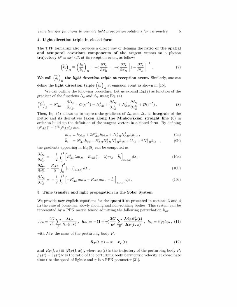
4. Light direction triple in closed form

The TTF formalism also provides a direct way of defining the ratio of the spatialand temporal covariant components of the tangent vectors to a photontrajectory kµ ≡ dxµ/dλ at its reception event, as follows(

ki

)B≡(kik0

)B

= −c ∂Te∂xiB

= −c ∂Tr∂xiB

[1− ∂Tr

∂tB

]−1. (7)

We call(ki

)B

the light direction triple at reception event. Similarly, one can

define the light direction triple(ki

)A

at emission event as shown in [15].

We can outline the following procedure. Let us expand Eq.(7) as function of thegradient of the functions ∆e and ∆r using Eq. (4)(ki

)B

= N iAB +

∂∆e

∂xiB+O(c−5) = N i

AB +∂∆r

∂xiB+N i

AB

∂∆r

∂x0B+O(c−5) . (8)

Then, Eq. (5) allows us to express the gradients of ∆e and ∆r as integrals of themetric and its derivatives taken along the Minkowskian straight line (6) inorder to build up the definition of the tangent vectors in a closed form. By defining(NAB)i = δij(NAB)j and

m,α ≡ h00,α + 2NkABh0k,α +N j

ABNkABhjk,α , (9a)

hi ≡ N iABh00 −N i

ABNjABN

kABhjk + 2h0i + 2N j

ABhij , (9b)

the gradients appearing in Eq.(8) can be computed as

∂∆r

∂xiB= − 1

2

∫ 1

0

[RiABλm,0 −RAB(1− λ)m,i − hi

]z−(λ)

dλ , (10a)

∂∆r

∂x0B=RAB

2

∫ 1

0

[m,0]z−(λ) dλ , (10b)

∂∆e

∂xiB= − 1

2

∫ 1

0

[−RiABµm,0 −RABµm,i + hi

]z+(µ)

dµ . (10c)

5. Time transfer and light propagation in the Solar System

We provide now explicit equations for the quantities presented in sections 3 and 4in the case of point-like, slowly moving and non-rotating bodies. This system can berepresented by a PPN metric tensor admitting the following perturbation hµν

h00 =2G

c2

∑P

MP

RP (t,x), h0i = −(1 +γ)

2G

c2

∑∑∑P

MPβiP (t)

RP (t, x), hij = δijγh00 , (11)

with MP the mass of the perturbing body P ,

RP (t,x) = x− xP (t) (12)

and RP (t,x) ≡ |RP (t, x)|, where xP (t) is the trajectory of the perturbing body P ;βiP (t) = viP (t)/c is the ratio of the perturbing body barycentric velocity at coordinatetime t to the speed of light c and γ is a PPN parameter [31].

Time transfer functions to validate light propagation solutions for astrometry 6

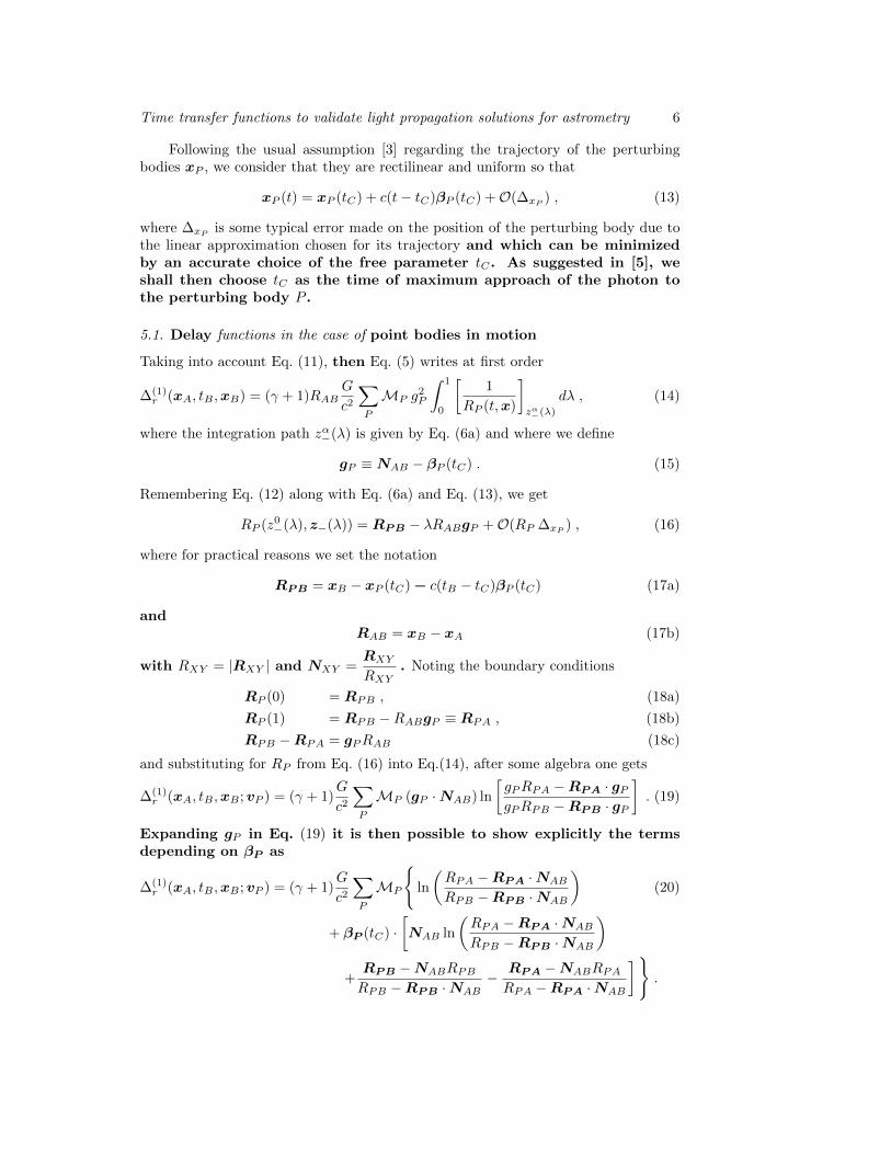
Following the usual assumption [3] regarding the trajectory of the perturbingbodies xP , we consider that they are rectilinear and uniform so that

xP (t) = xP (tC) + c(t− tC)βP (tC) +O(∆xP ) , (13)

where ∆xP is some typical error made on the position of the perturbing body due tothe linear approximation chosen for its trajectory and which can be minimizedby an accurate choice of the free parameter tC . As suggested in [5], weshall then choose tC as the time of maximum approach of the photon tothe perturbing body P .

5.1. Delay functions in the case of point bodies in motion

Taking into account Eq. (11), then Eq. (5) writes at first order

∆(1)r (xA, tB ,xB) = (γ + 1)RAB

G

c2

∑P

MP g2P

∫ 1

0

[1

RP (t,x)

]zα−(λ)

dλ , (14)

where the integration path zα−(λ) is given by Eq. (6a) and where we define

gP ≡NAB − βP (tC) . (15)

Remembering Eq. (12) along with Eq. (6a) and Eq. (13), we get

RP (z0−(λ), z−(λ)) = RPB − λRABgP +O(RP ∆xP ) , (16)

where for practical reasons we set the notation

RPB = xB − xP (tC)− c(tB − tC)βP (tC) (17a)

andRAB = xB − xA (17b)

with RXY = |RXY | and NXY =RXY

RXY. Noting the boundary conditions

RP (0) = RPB , (18a)

RP (1) = RPB −RABgP ≡ RPA , (18b)

RPB −RPA = gPRAB (18c)

and substituting for RP from Eq. (16) into Eq.(14), after some algebra one gets

∆(1)r (xA, tB ,xB ;vP ) = (γ + 1)

G

c2

∑P

MP (gP ·NAB) ln

[gPRPA −RPA · gPgPRPB −RPB · gP

]. (19)

Expanding gP in Eq. (19) it is then possible to show explicitly the termsdepending on βP as

∆(1)r (xA, tB ,xB ;vP ) = (γ + 1)

G

c2

∑P

MP

{ln

(RPA −RPA ·NAB

RPB −RPB ·NAB

)(20)

+ βP (tC) ·[NAB ln

(RPA −RPA ·NAB

RPB −RPB ·NAB

)+RPB −NABRPBRPB −RPB ·NAB

− RPA −NABRPARPA −RPA ·NAB

]}.

Time transfer functions to validate light propagation solutions for astrometry 7

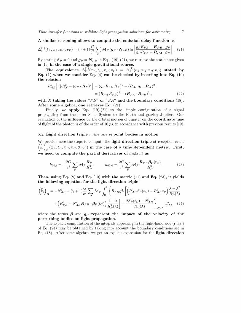
A similar reasoning allows to compute the emission delay function as

∆(1)e (tA,xA,xB ;vP ) = (γ + 1)

G

c2

∑P

MP (gP ·NAB) ln

[gPRPB +RPB · gPgPRPA +RPA · gP

]. (21)

By setting βP = 0 and gP = NAB in Eqs. (19)-(21), we retrieve the static case givenin [19] in the case of a single gravitational source.

The equivalence ∆(1)r (xA, tB ,xB ;vP ) = ∆

(1)e (tA,xA,xB ;vP ) stated by

Eq. (1) when we consider Eq. (4) can be checked by inserting into Eq. (19)the relation

R2AB

[g2PR

2X − (gP ·RX)2

]= (gP RAB RX)2 − (RABgP ·RX)2

= (RPARPB)2 − (RPA ·RPB)2 , (22)

with X taking the values ”PB” or ”PA” and the boundary conditions (18).After some algebra, one retrieves Eq. (21).

Finally, we apply Eqs. (19)-(21) to the simple configuration of a signalpropagating from the outer Solar System to the Earth and grazing Jupiter. Ourevaluation of the influence by the orbital motion of Jupiter on the coordinate timeof flight of the photon is of the order of 10 ps, in accordance with previous results [19].

5.2. Light direction triple in the case of point bodies in motion

We provide here the steps to compute the light direction triple at reception event(ki

)B

(xA, tB ,xB ,xP ,βP , γ) in the case of a time dependent metric. First,

we need to compute the partial derivatives of h00(x, t) as

h00,i = −2G

c2

∑P

MPRiPR3P

, h00,0 =2G

c2

∑P

MPRP · βP (tC)

R3P

. (23)

Then, using Eq. (8) and Eq. (10) with the metric (11) and Eq. (23), it yieldsthe following equation for the light direction triple(ki

)B

= −N iAB + (γ + 1)

G

c2

∑P

MP

∫ 1

0

{RABg

2P

[(RABβ

iP (tC)−RiABgP

)λ− λ2R3P (λ)

+(RiPB −N i

ABRPB · βP (tC)) 1− λR3P (λ)

]+

2βiP (tC)−N iAB

RP (λ)

}zα−(λ)

dλ , (24)

where the terms β and gP represent the impact of the velocity of theperturbing bodies on light propagation.

The explicit computation of the integrals appearing in the right-hand side (r.h.s.)of Eq. (24) may be obtained by taking into account the boundary conditions set inEq. (18). After some algebra, we get an explicit expression for the light direction

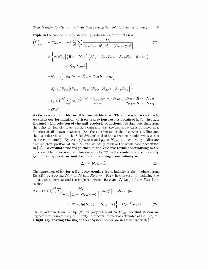
Time transfer functions to validate light propagation solutions for astrometry 8

triple in the case of multiple deflecting bodies in uniform motion as(ki

)B

= −N iAB + (γ + 1)

G

c2

∑P

MP

RABRPB

[R2PBg

2P − (RPB · gP )2

] (25)

×

{gPN

iAB

[(RPB ·NAB

)(R2PB −RPARPB −RABRPB · βP (tC)

)−R2

PBRABg2P

]+RiPBg

2P

[RPBRPA −R2

PB +RABRPB · gP]

+ βiP (tC)RPB

[(RPA −RPB)(RPB ·NAB) +RPBRAB

]}

+ (γ + 1)G

c2

∑P

MPβiP (tC)−N i

ABβP (tC) ·NAB

RABgPlnRPB +RPB ·NAB

RPA +RPA ·NAB

+O(c−4) .

As far as we know, this result is new within the TTF approach. In section 6,we check our formulation with some previous results obtained in [3] throughthe analytical solution of the null-geodesic equations. We shall note that, fromthe point of view of the astrometric data analysis, the last equation is obtained as afunction of all known quantities (i.e. the coordinates of the observing satellite andthe mass distribution in the Solar System) and of the astrometric unknown (i.e. thesource coordinates). By setting βP = 0 and gP = NAB , the perturbing bodies arefixed at their position at time tC and we easily retrieve the static case presentedin [17]. To evaluate the magnitude of the velocity terms contributing to thedirection of light, we use the definition given by [22] in the context of a sphericallysymmetric space-time and for a signal coming from infinity as

∆χ ≈ |NAB × kB | . (26)

The expression of kB for a light ray coming from infinity is then deduced fromEq. (25) by setting NAB ≡ N and RPA ≈ −RAB in this case. Introducing theimpact parameter bP and the angle α between RPB and N we get bP = RPB sinα,so that

∆χ = (γ + 1)G

c2

∑P

MP

R2PB

[g2P − (NPB · gP )2

]{bP g2P [1 +NPB · gP]

+ |N × βP |RPB(1−NPB ·N

)}+O(c−4, R−1AB) . (27)

The logarithmic term in Eq. (25) is proportional to RAB, so that it can beneglected for sources at quasi-infinity. Moreover, numerical estimates of Eq. (27) fora light ray grazing the major Solar System bodies are in agreement with [5].

Time transfer functions to validate light propagation solutions for astrometry 9

6. Relativistic astrometric models at the cross-checking point

The astrometric core solution of the forthcoming Gaia mission [9] will be performed bythe Astrometric Global Iterative Solution (AGIS) software [33]. At the same time, anindependent verification unit for AGIS called Global Sphere Reconstruction (GSR) [34]has been set within the Gaia Data Processing and Analysis Consortium (DPAC). Sinceboth pipelines are intended to operate on the same real data, the comparison of theirresults is mandatory in order to validate the final astrometric catalog. In order tokeep the two software as separate as possible, two different relativistic modelings oflight propagation have been implemented: AGIS relies on GREM [5], while GSRimplements RAMOD [14]. Both models are internally consistent at the µaslevel required by Gaia. However, due to their different conception, agood reciprocal understanding is a complex task and a comparison effortis already in place, focusing on the modeling of the astrometric observableand the aberration [35]. We contribute to this study by establishing here anoriginal procedure to cross-check our results on the gravitational deflectionof light with those of these Gaia models. In particular, concerning GREM,we compare our model to its seminal study [3] which we will name KK92 inthe following. This choice allows us to check both the results of section 5and the GREM model, which is a version of KK92 accurate at the µaslevel.

6.1. KK92 modeling

KK92 describes light propagation in a gravitational system close to the one describedby the metric (11) , where the trajectory of the perturbing bodies is given byEq. (13). Considering only the terms relevant for our purpose and using our notation,the trajectory of the photon can be written as

xi(t) = xi(tB) + cσi(t− tB) + ∆xi(t, xi, tB , xiB) , (28)

where (tB , xi(tB)) are the reception coordinates, σ is a normalized vector giving the

unperturbed direction of light at past null infinity and the gravitational perturbationis given by

∆xi = − 2G

c2

∑P

MP{giP ln

[gP ·RP (t) + gPRP (t)

gP ·RPB + gPRPB

]+

(σ ×RP (t)× gP )i

gPRP (t)− gP ·RP (t)

− (σ ×RPB × gP )i

gPRPB − gP ·RPB

}. (29)

The TTF formalism being designed for light propagation between two points locatedat finite distance, one has first to set the boundary condition

x(xB ,σ,∆t) = xA (30)

in Eq. (28) to provide the ”crossing trajectory equation”

xi(tA) = xi(tB)− c∆t σi + ∆xi(∆t, xiB , σi) , (31)

where ∆t ≡ tB − tA represents the lapse of coordinate time between the emissionand reception of the signal. In the following, Eqs. (28)-(31) will be used to find the

Time transfer functions to validate light propagation solutions for astrometry 10

equivalence of KK92 and TTF for the coordinate time of flight and the directiontriple at reception coordinates. If the velocity terms are neglected inEq. (13), we then retrieve the equivalence in the GREM case and at theµas accuracy.

6.1.1. Coordinate time of flight. Let us state the formal development

∆t =∑i

∆t(i) , (32)

where ∆t(n) is of order O(c−n). Substituting for ∆t from Eq. (32) into Eq. (31) andidentifying terms of the same order, we find

∆t(1) =RABc

, (33a)

∆t(2) = NAB ·∆x(∆t, xiB , σi) (33b)

= − 2G

c2

∑P

MP (gP ·NAB) ln

[gP ·RPA + gPRPAgP ·RPB + gPRPB

],

where we used the property σ·σ = 1 and noted thatNAB ·(NAB×RX×gP ) = 0. UsingEq. (22) shows that Eq. (33) is strictly equivalent to Eq. (4) when the gravitationaldelay is given by Eq. (19) with γ = 1.

6.1.2. Light direction triple. The relation between the tangent vectors kµ =dxµ

dλ

and the photon velocity xi used in KK92 is obtained byxi

c=

dxi/dλ

dx0/dλ=

ki

k0. It

follows that

ki =kik0

=gijk

j + g0ik0

g00k0 + g0iki=(g0i + gij

kj

k0)(g00 + g0i

ki

k0)−1

= − xi

c− 2h00σ

i − (δij + σiσj)h0j +O(c−4) . (34)

The computation ofxi

cis obtained by deriving the photon trajectory in Eq. (28)

with respect to coordinate time. Its application at reception coordinates (tB ,xB)gives

xiBc

= σi +∆xiBc

, (35)

where ∆xi represents the gravitational perturbation to the photon direction

∆xiBc

= − 2G

c2

∑P

MPgPRPB

{giP +

(NAB ×RPA × gP )i

gPRPB − gP ·RPB

}. (36)

Let us state the formal development

σ =∑i

σ(i) , (37)

Time transfer functions to validate light propagation solutions for astrometry 11

where σ(i) is of order O(c−n). Substituting for σ from Eq. (37) into Eq. (31) andidentifying all terms of the same order, we find

σi(1) =xiB − xiARAB

= N iAB , (38a)

σi(2) = − 1

RAB

[δij −N i

ABNjAB

]∆xj(∆t, xjB , σ

j) , (38b)

where we used the property σ ·σ = 1. Using Eq. (22) and after some algebra, we findthe following relation

(σ ×RPA × gP )i

gPRPA − (gP ·RPA)− (σ ×RPB × gP )i

gPRPB − (gP ·RPB)= (39)

gP (σ ×RPB × gP )i

R2PAR

2PB − (RPA ·RPB)2

[RPA −RPB − gPRAB

].

Substituting for ∆xi from Eq. (29) into Eq. (38) with the relation given in Eq. (39),we obtain

σi = N iAB −

2G

c2

∑P

MP

RAB

[(NAB ×RPB × gP )i

g2PR2PB − (gP ·RPB)2

(gPRPA − gPRPB − g2PRAB

)+(giP −N i

ABNjABg

jP

)ln

(gPRPB − gP ·RPB

gPRPA − gP ·RPA

)]+O(c−4) . (40)

It is then straightforward to check that Eq. (25) is equivalent to Eq. (34) when usingEq. (35), Eq. (36), Eq. (40) and the metric tensor (11) at reception event.

6.2. RAMOD modeling

Based on a complete PM background [36], RAMOD has been solved explicitly inthe 1PM approximation needed for GSR [37]. RAMOD always relies on measurablequantities with respect to a local barycentric observer along the light ray [6]. Theunknown is then the local line-of-sight, representing the direction of the lightray in the rest space of the observer u, and defined as

¯α = − kα

uβkβ− uα , (41)

where kµ represent the tangent vectors to the null-geodesic. In this formalism, thenull-geodesic equation transforms, according to the measurement protocol procedure,into a set of coupled nonlinear differential equations, called ”master equations”

d¯0

dζ− ¯i ¯jh0j,i −

1

2h00,0 = 0 , (42a)

d¯k

dζ− 1

2¯k ¯i

(¯jhij,0 − h00,i

)+ ¯i ¯j

(hkj,i −

1

2hij,k

)+ ¯i

(hk0,i + hki,0 − h0i,k

)− 1

2h00,k − ¯k ¯ih0i,0 + hk0,0 = 0 , (42b)

where ζ is a parameter along the null-geodesic. Comparisons between RAMOD andother PM/PN astrometric models can be found in [36], where the author showshow RAMOD master equations recover the analytical linearized case used in [24]once converted in a coordinate form while in [35] the authors present a study of the

Time transfer functions to validate light propagation solutions for astrometry 12

aberration in RAMOD and GREM. An analytical cross-check has not been done yetwith the TTF. We perform it in the case of a fully analytical solution accurate atthe GREM level [37], described by the gravitational perturbation (11), where weset βP = 0, γ = 1 and the position of the perturbing bodies is fixed at thetime of maximum approach with the photon tC .

Indeed, the inclusion of the velocities in RAMOD requires a carefulapplication of the measurement protocol so that the case of a field of bodiesin uniform motion needs to be treated in a separate and exhaustive paper.

6.2.1. Coordinate time of flight. The computation of the coordinate time of flight∆t can be obtained within RAMOD by considering the time component of the localobserver u as

u0 ≡ cdt

dζ= 1 +

h002

+O(c−4) , (43)

where ζ is a parameter along the null-geodesic [14]. Inserting Eq. (11) takenat the chosen approximation into Eq. (43) and integrating between the emissionζA and the reception ζB , we get

c∆t =

∫ ζB

ζA

(1 +

G

c2

∑P

MP1

RP (ζ)

)dζ +O(c−4)

= ∆ζ +G

c2

∑P

MP lnRPB +NAB ·RPBRPA +NAB ·RPA

+O(c−4) , (44)

where ∆ζ ≡ ζB − ζA and we used definitions (17) and (18) with βP = 0. We neednow an explicit expression for ∆ζ. First, we rewrite following our notation Eq. (18)of [37]

¯kB =

xkB − xkA∆ζ

+2G

c2

∑P

MP

{NkAB

2

[1

∆ζln

[NAB ·RPB +RPBNAB ·RPA +RPA

]− 1

RPB

]+dkBd2B

[−NAB ·RPB

RPB+RPB −RPA

∆ζ

]}+O

(c−4)

(45)

with dB ≡ RPB −NAB(RPB ·NAB). Then, using the relation dB ·NAB = 0 andthe normalisation condition ¯α ¯

α = gαβ ¯α ¯β = 1 on Eq. (45), we obtain

¯kB

¯kB = 1− h00

∣∣∣B

+O(c−4) =R2AB

∆ζ2+

2G

c2

∑P

MP (46)

×{RAB∆ζ2

ln

[(NAB ·RPB) +RPB(NAB ·RPA) +RPA

]− RABRPB∆ζ

}+O

(c−4).

Following Eq. (44), we assume that ∆ζ admits a PN expansion

∆ζ = RAB + ∆ζ(2) +O(c−3) , (47)

where ∆ζ(2) is of order O(c−2). Substituting for ∆ζ from Eq. (47) into Eq. (46) andidentifying the terms of the same order, we get straightforwardly

∆ζ(2) =G

c2

∑P

MP ln

[RPB +NAB ·RPBRPA +NAB ·RPA

]. (48)

Finally, substituting for ∆ζ from Eq. (47) and Eq. (48) into Eq. (44) we retrieve theShapiro term of Eq. (19) with βP = 0.

REFERENCES 13

6.2.2. Light direction triple. The relation between the light direction tripleki and the local line-of-sight ¯i at reception point xB is obtained by expandingEq. (41) with the metric (11) taken at the chosen approximation. ConsideringEq. (43) for u0, we get

¯iB = −

ki

u0k0

∣∣∣∣∣B

= −(ki

)B

[1−

3

2h00

∣∣∣B

]+O(c−3) ≈ −

(ki

)B

[1−

3G

c2

∑∑∑P

MP

RPB

].

(49)

Substituting for(ki

)B

from Eq. (25) into Eq. (49) with βP = 0, the reader

can easily retrieve Eq. (45) where ∆ζ is given by Eqs. (47)-(48).

7. Conclusions

This paper provides the coordinate time of flight of a photon between two pointsat finite distance and the direction triple at its reception coordinates asintegrals taken along the Minkowskian straight line between its emissionand reception points. It is remarkable that Eq.(5) and Eqs. (8)-(10) give thesequantities in closed form as function of just few parameters and for any metrictensor describing a weak gravitational field in the PPN framework. We use ourformulae to provide a first application of the TTF formalism in the case of the time-dependent metric tensor (11), describing a system of point bodies in uniformmotion. Eqs. (19)-(21) and Eq. (25) extend the results previously obtained in [18] andare used here to find a procedure to relate and compare three independent approachesto relativistic light propagation. Section 6.1 shows that the results of TTF and KK92are equivalent at 1PN in a time-dependent gravitational field. The comparisonwith GREM at the µas level required for the Gaia mission can then beretrieved by fixing the positions of the perturbing bodies at their closestapproach with the photon while the equivalence of the results of TTF andRAMOD at the same accuracy level is demonstrated in section 6.2. Such across-checking procedure enters the same thread of model comparison started in [35],which is essential to fully understand the observational data coming from Gaia in acommon experimental context.

Acknowledgments

The authors are grateful to P. Teyssandier for fruitful discussions and suggestions.S. Bertone is Ph.D. student under the UIF/UFI (French-Italian University) programand thanks UIF/UFI for the financial support of this work. S. Bertone, C. Le Poncin-Lafitte and M.-C. Angonin are grateful to the financial support of CNRS/GRAMand CNES. The work of M. Crosta and A. Vecchiato has been partially funded byASI under contract to INAF I/058/10/0 (Gaia Mission - The Italian Participation toDPAC).

References

[1] Soffel M H, Wu X, Xu C and Mueller J 1991 Astronomical Journal 101 2306–2310

REFERENCES 14

[2] Moyer 2000 Formulation for Observed and Computed Values of Deep SpaceNetwork Data Types for Navigation Monograph 2 Deep Space Communicationsand Navigation Series

[3] Klioner S A and Kopeikin S M 1992 Astronomical Journal 104 897–914

[4] Soffel M, Klioner S A, Petit G, Wolf P, Kopeikin S M, Bretagnon P, BrumbergV A, Capitaine N, Damour T, Fukushima T, Guinot B, Huang T Y, LindegrenL, Ma C, Nordtvedt K, Ries J C, Seidelmann P K, Vokrouhlicky D, WillC M and Xu C 2003 Astronomical Journal 126 2687–2706 (Preprint arXiv:

astro-ph/0303376)

[5] Klioner S A 2003 Astronomical Journal 125 1580–1597

[6] de Felice F, Crosta M, Vecchiato A, Lattanzi M and Bucciarelli B 2004Astrophysical Journal 607 580–595 (Preprint arXiv:astro-ph/0401637)

[7] Bini D, Crosta M T and de Felice F 2003 Classical and Quantum Gravity 204695–4706

[8] Klioner S A 2004 Physical Review D 69 124001 (Preprint arXiv:astro-ph/

0311540)

[9] Bienayme O and Turon C 2002 EAS Publications Series 2

[10] Misner C, Thorne K and Wheeler J 1973 Gravitation (San Francisco: W. H.Freeman)

[11] Kopeikin S M and Makarov V V 2007 Physical Review D 75 062002 (PreprintarXiv:astro-ph/0611358)

[12] Minazzoli O and Chauvineau B 2011 Classical and Quantum Gravity 28 085010(Preprint 1007.3942)

[13] Deng X M and Xie Y 2012 Physical Review D 86 044007 (Preprint 1207.3138)

[14] de Felice F, Vecchiato A, Crosta M T, Bucciarelli B and Lattanzi M G 2006Astrophysical Journal 653 1552–1565 (Preprint arXiv:astro-ph/0609073)

[15] Le Poncin-Lafitte C, Linet B and Teyssandier P 2004 Classical and QuantumGravity 21 4463–4483 (Preprint arXiv:gr-qc/0403094)

[16] Bertone S and Le Poncin-Lafitte C 2012 Memorie della Societa AstronomicaItaliana 83 1020 (Preprint 1111.1325)

[17] Teyssandier P and Le Poncin-Lafitte C 2008 Classical and Quantum Gravity 25145020 (Preprint 0803.0277)

[18] Le Poncin-Lafitte C and Teyssandier P 2008 Physical Review D 77 044029(Preprint 0711.4292)

[19] Linet B and Teyssandier P 2002 Physical Review D 66 024045 (Preprint arXiv:

gr-qc/0204009)

[20] Klioner S and Zschocke S 2010 Classical and Quantum Gravity 27 075015(Preprint 1001.2133)

[21] Ashby N and Bertotti B 2010 Classical and Quantum Gravity 27 145013 (Preprint0912.2705)

[22] Teyssandier P 2012 Classical and Quantum Gravity 29 245010 (Preprint 1206.

6309)

[23] Teyssandier P and Linet B 2012 Memorie della Societa Astronomica Italiana 831024

REFERENCES 15

[24] Kopeikin S M and Schafer G 1999 Physical Review D 60 124002 (PreprintarXiv:gr-qc/9902030)

[25] Kopeikin S and Mashhoon B 2002 Physical Review D 65 064025 (PreprintarXiv:gr-qc/0110101)

[26] de Felice F and Bini D 2010 Classical Measurements in Curved Space-Times(Cambridge Monographs on Mathematical Physics)

[27] Will C M 2006 Living Reviews in Relativity 9 URL http://www.livingreviews.

org/lrr-2006-3

[28] Synge J L 1960 Relativity: The General Theory (Amsterdam: North-HollandPubl. Co.) russian translation: IL (Foreign Literature), Moscow, 1963

[29] Hees A, Lamine B, Reynaud S, Jaekel M T, Le Poncin-Lafitte C, Lainey V, FuzfaA, Courty J M, Dehant V and Wolf P 2012 Classical and Quantum Gravity 29235027 (Preprint 1201.5041)

[30] Lambert S B and Le Poncin-Lafitte C 2009 Astronomy and Astrophysics 499331–335 (Preprint 0903.1615)

[31] Will C M 1993 Theory and Experiment in Gravitational Physics

[32] Teyssandier P, Le Poncin-Lafitte C and Linet B 2008 A universal tool fordetermining the time delay and the frequency shift of light: Synge’s worldfunction Lasers, Clocks and Drag-Free Control: Exploration of RelativisticGravity in Space (Astrophysics and Space Science Library vol 349) ed H Dittus,C Lammerzahl, & S G Turyshev p 153 (Preprint 0711.0034)

[33] Lindegren L, Lammers U, Hobbs D, O’Mullane W, Bastian U and Hernandez J2012 Astronomy & Astrophysics 538 A78 (Preprint 1112.4139)

[34] Vecchiato A, Abbas U, Bandieramonte M, Becciani U, Bianchi L, Bucciarelli B,Busonero D, Lattanzi M G and Messineo R 2012 The global sphere reconstructionfor the gaia mission in the astrometric verification unit Society of Photo-OpticalInstrumentation Engineers (SPIE) Conference Series vol 8451

[35] Crosta M and Vecchiato A 2010 Astronomy and Astrophysics 509 A37

[36] Crosta M 2011 Classical and Quantum Gravity 28 235013 (Preprint 1012.5226)

[37] Crosta M 2013 ArXiv e-prints (Preprint 1305.4824)

[38] Bini D, Crosta M, de Felice F, Geralico A and Vecchiato A 2013 Classical andQuantum Gravity 30 045009