A Model-Based Monitoring and Diagnosis System for a Space-Based Astrometry Mission

DR

AFT

A Model-Based Monitoring Systemfor a Space-Based Astrometry

Mission

Inauguraldissertationzur Erlangung des akademischen Gradeseines Doktors der Naturwissenschaften

der Universitat Mannheim

vorgelegt von

Dr. rer. nat.Alexey Pavlov

aus Moskau

Mannheim, 2006

DR

AFT

Dekan: Professor Dr. Matthias Krause, Universitat MannheimReferent: Professor Dr. Guido Moerkotte, Universitat MannheimKorreferent: Professor Dr. Rainer Spurzem, Universitat Heidelberg

Tag der mundlichen Prufung: 15. Marz 2006

DR

AFT

Abstract

Astrometric space missions like Hipparcos, DIVA, Gaia have to simultaneously de-termine a tremendous number of parameters concerning astrometric and other stellarproperties, the satellite’s attitude as well as the geometric and photometric calibration ofthe instrument. To reach the targeted level of precision for these missions many monthsof observational data have to be incorporated intos a global, coherent and interleaveddata reduction. It is inevitable that a daily data reduction process is required in order tojudge if the level of precision of the stellar, attitude and instrument parameters achieveits targeted level. This sophisticated data analysis is the in-depth scientific assessmentof the quality of all observations within about 24 hours after its reception. It is basedon the very complicated procedure ”First Look preprocessing” (more known as a Great-Circle reduction from Hipparcos) that provides a one-dimensional, self-consistent andsimultaneous solution of the attitude, the instrument calibration and celestial sourceparameters. For this purpose one needs to process all the 24-hours-data, a task whichcan be only performed at the Data Center with its computer resources. On the otherhand, it is necessary and reasonable to process the observations at the ground Space Op-erations Center for a quick discovery of delicate changes in the spacecraft performancein the quasi-real time constraints (15÷ 30 min after data reception).

For this latter purpose, the concept of a model-based monitoring system has beendeveloped that comprises activities concerning scientific data health of an astrometricalsatellite which can not be guaranteed by only standard procedures applied to typicalspace missions. This monitoring system, called Science Quick Look (ScQL), performsthe preliminary scientific assessment of the instrument and proper astrometric working ofthe spacecraft at the (coarse) level of precision attainable at this stage. The prototype ofthis software is designed in the framework of the DIVA project, providing monitoring,diagnostic and visualization tools. It performs the first scientific assessment of thegeometric stability of the instrument and proper working of the spacecraft. The processof the monitoring is based on a model of the Galaxy, on the structure and behavior ofthe components of the spacecraft and its scanning strategy. The system incorporates asimulator of the observations of stars – a core of our model, that allows to mimic thework of the on-board software and to simulate star transits.

The results of an evaluation of our system look very promising, so we plan to pursuefurther studies in this area. As the DIVA project was stopped, we will adopt ourapproach to the next space-based astrometry mission, Gaia, which will be launched in2012. Indeed, many aspects for the rapid assessment of payload and spacecraft health,developed in this work in the framework of DIVA project, are analogous to those inGaia due to the fact that the basic principle and geometry of the measurements are thesame.

A successful completion of the ScQL prototype for the DIVA mission provides thebasis for our belief that a ScQL monitoring system for the larger project – Gaia – is

DR

AFT

iv

achievable in terms of the developed concept. Building a ScQL monitoring system forGaia therefore would become a lot easier if the important steps have already been donein the DIVA project. It is evident, however, that this work has to evolve and grow,along with the concept of the Gaia satellite.

DR

AFT

Zusammenfassung

In astrometrischen Weltraummissionen wie Hipparcos, DIVA oder Gaia muss eineVielzahl von Parametern gleichzeitig bestimmt werden, wie astrometrische und an-dere stellare Eigenschaften, die Lage des Satelliten sowie die geometrische und pho-tometrische Kalibrierung der Instrumente. Um das Prazisionsniveau zu erreichen, dasin diesen Missionen angestrebt wird, mussen die uber Monate gesammelten Daten ineine globale und koharente Datenreduktionen eingebunden werden. Der Prozess dertaglichen Datenreduktion ist unbedingt notwendig, um einschatzen zu konnen, ob derangestrebte Prazisionsgrad der stellaren Parameter, der Lage des Satelliten und der In-strumente erreicht ist. Mit dieser anspruchsvollen Datenanalyse wird die Qualitat allerDaten innerhalb von 24 Stunden nach deren Empfang mit wissenschaftlichen Meth-oden grundlich uberpruft. Sie basiert auf einer komplizierten Prozedur, First LookPreprocessing genannt. Diese Prozedur liefert eine eindimensionale, selbstkonsistenteund simultane Losung fur die Parameter der Lage des Satelliten, der Kalibrierung derInstrumente und der kosmischen Objekte. Diese Analyse kann nur im Data Centerdurchgefuhrt werden, weil hier die entsprechenden Computerressourcen zur Verfugungstehen. Andererseits ist es notwendig und vernunftig, die Beobachtungen auf der Erdeim Space Operations Center durchzufuhren, weil auf diese Weise minimale Abweichun-gen in der Performanz des Satelliten in Quasi-Echtzeit (15-30 min. nach Empfang derDaten) rasch entdeckt werden konnen.

Zu diesem Zweck wurde das Konzept eines modellbasierten Uberwachungssystemsentwickelt. Es umfasst alle Aspekte der Korrektheit der wissenschaftlichen Daten einesastrometrischen Satelliten, die mit den Standardprozeduren gewohnlicher Weltraum-missionen nicht garantiert werden konnen. Dieses Uberwachungssystem, Science QuickLook (ScQL) genannt, uberpruft schon im Voraus, ob das Instrument und der Satellitrichtig funktionieren, auf dem Prazisionsniveau, das in diesem Stadium moglich ist. DerPrototyp dieser Software wurde im Rahmen des DIVA-Projekts entwickelt und bietetTools fur Uberwachung, Diagnose und Visualisierung. Die Software fuhrt eine erstewissenschaftliche Beurteilung der geometrischen Stabilitat des Instruments und der kor-rekten Funktion des Satelliten durch. Der Ablauf der Kontrolle basiert auf einem Modellder Galaxie sowie auf der Struktur und dem Verhalten der Komponenten des Satellitenund seiner Strategie. Das System enthalt einen Simulator fur die Beobachtungen vonSternen - der Kern unseres Modells, der es ermoglicht, die Arbeit der Software an Bordzu imitieren und die Sterntranists zu simulieren.

Eine Bewertung unseres Systems lieferte viel versprechende Ergebnisse, deshalb pla-nen wir weitere Studien auf diesem Gebiet. Da das DIVA-Projekt abgebrochen wurde,werden wir unseren Ansatz bei der nachsten astrometrischen Weltraummission, Gaia,anzuwenden versuchen, die 2012 starten soll. Viele Schritte zur raschen Uberprufungvon Belastung und Zustand der Raumsonde, die in dieser Arbeit fur das DIVA-Projektentwickelt wurden, entsprechen denen in GAIA, da das Grundprinzip und die Geometrie

DR

AFT

vi

der Messungen in beiden Projekten gleich sind.Im Rahmen dieser Arbeit wurde die Entwicklung eines ScQL-Prototyps fur DIVA

erfolgreich abgeschlossen. Deshalb sind wir der Uberzeugung, dass es moglich ist, inner-halb des bestehenden Konzepts ein ScQL-Uberwachungssystem fur Gaia zu entwickeln.Es bleibt jedoch anzumerken, dass eine solche Arbeit gemeinsam mit dem Konzept desGaia-Satelliten wachsen und sich weiter entwickeln muss.

DR

AFT

Preface and acknowledgments

This thesis is submitted in fulfillment of the requirements for the Doctor of Natural Sci-ences at the Lehrstuhl fur Praktische Informatik III, Universitat Mannheim, Germany.The work has been carried out in the period from January 2002 to January 2005 underthe supervision of Professor Guido Moerkotte.

The thesis considers the design of a monitoring system for the rapid assessment ofpayload and spacecraft performance using a model-based approach. It can be appliedto an astrometrical scanning satellite where the health of the scientific data can not beguaranteed by only standard monitoring procedures applied to typical space missions.The results presented in this work are generally based on the involvement into the DIVA

project.

Looking back over the last three years, reminding me how this work depended on theefforts and contributions of many people. I would like to acknowledge all those peoplewho played an integral role in helping me to reach the completion of my dissertation.Without their support and friendship I would not have had the great pleasure of writingthis page.

Mannheim University

First of all, I am gratefully indebted to my supervisor Professor Guido Moerkotte forhis guidance throughout this thesis. His capacity to combine the penetrating criticismand the offering direction as well as his academic experience helped me to establish theoverall direction of the research and to remain focused on achieving my goal.

I would further like to thank very much Dr. Sven Helmer for his permanent advicesduring the endeavor of my doctoral research. His observations and comments on mydrafts significantly improved the concept of my thesis and helped me to move forwardwith the investigation in depth.

Astronomisches-Rechen Institut (ARI)

I would like particularly to mention Dr. Elena Schilbach and Dr. Siegfried Roser forgiving me the opportunity to participate in the preparation of the DIVA space missionand for their unending support during my work on this project. I am grateful for theirpreparedness to enlighten me on various aspects of the project, without their help thelearning curve would have been very much flatter.

I am extremely grateful to Dr. Michael Biermann for helping me getting started withthe task of the science quick look diagnosis and and for his great contribution.

I would like to express my gratitude to Dr. Sonja Hirte for your invaluable help as well

DR

AFT

viii

as informal support and encouragement.

I also extend my sincere gratitude to Dr. Ulrich Bastian who helped me to learn aboutthe features of the astrometrical space projects during my first year at ARI. I am alsograteful that he gave me the opportunity for being shortly involved in the space projectGaia and to visit the Gaia meeting in Barcelona-2003, it provided me with a wealth ofinformation and insights.

I am grateful to Frau Helga Ballmann from ARI and Frau Simone Seeger from MannheimUniversity for assisting me all the time in the real world of the German society. I wouldhave been lost without their help.

Institute of Astronomy, Russian Academy of Science (INASAN)

I would like to mention Dr. Nina V. Kharchenko and Dr. Anatoly E. Piskunov whoencouraged me to burn the midnight oil, so that I could manage (almost!) to keep mydeadline. I have certainly benefitted from extensive discussions with them during thelast months of my stay at ARI. The invaluable help in understanding different aspectsof the modern Galaxy model was highly appreciated.

Klaus Tschira Foundation

I gratefully acknowledge the financial support from the Klaus Tschira Foundation.

It would, of course, be completely amiss for me to end my acknowledgments withoutrecognizing the immense contribution that my parents have made to my work. De-spite living about 2000 km away, they are constantly in my thoughts and their love andsupport have been a major stabilizing force over these past three years. Their unques-tioning faith in me and my abilities has helped to make all this possible and for that,and everything else, I dedicate this thesis to them.

DR

AFT

Contents

1 Introduction 11.1 Sky . . . . . . . . . . . . . . . . . . . . . . . . . . . . . . . . . . . . . . . 11.2 Astrometry . . . . . . . . . . . . . . . . . . . . . . . . . . . . . . . . . . 31.3 Astrometric satellites . . . . . . . . . . . . . . . . . . . . . . . . . . . . . 61.4 DIVA-mission overview and main instrument . . . . . . . . . . . . . . . . 81.5 Motivation for rapid assessment of payload and spacecraft health in the

framework of an astrometry mission. Science Quick Look. . . . . . . . . . 111.6 The Goal of Ph.D. Thesis . . . . . . . . . . . . . . . . . . . . . . . . . . 121.7 Guide to the Dissertation . . . . . . . . . . . . . . . . . . . . . . . . . . . 13

2 Monitoring systems 172.1 Monitoring and alarms . . . . . . . . . . . . . . . . . . . . . . . . . . . . 172.2 Artificial intelligence techniques for monitoring. Related work. . . . . . . 19

2.2.1 Symptom-based approaches . . . . . . . . . . . . . . . . . . . . . 192.2.2 Model-Based Reasoning . . . . . . . . . . . . . . . . . . . . . . . 222.2.3 Fault detection and isolation . . . . . . . . . . . . . . . . . . . . . 26

2.3 Summary . . . . . . . . . . . . . . . . . . . . . . . . . . . . . . . . . . . 26

3 From Requirements to Diagnostic Solutions 293.1 Requirements of the Science Quick Look (ScQL) . . . . . . . . . . . . . . 293.2 The design of the ScQL . . . . . . . . . . . . . . . . . . . . . . . . . . . . 353.3 Summary . . . . . . . . . . . . . . . . . . . . . . . . . . . . . . . . . . . 41

4 Star transit simulation 434.1 The Sky . . . . . . . . . . . . . . . . . . . . . . . . . . . . . . . . . . . . 44

4.1.1 Equatorial coordinates; the International Celestial Reference Sys-tem (ICRS) . . . . . . . . . . . . . . . . . . . . . . . . . . . . . . 45

4.1.2 The Ecliptic Coordinate System . . . . . . . . . . . . . . . . . . . 474.1.3 Galactic Coordinates . . . . . . . . . . . . . . . . . . . . . . . . . 474.1.4 Coordinate transformations . . . . . . . . . . . . . . . . . . . . . 48

4.2 The model of Galaxy . . . . . . . . . . . . . . . . . . . . . . . . . . . . . 494.2.1 Stellar distribution and simulation of a map of the sky . . . . . . 49

ix

DR

AFT

x CONTENTS

4.2.2 Simulation of the stellar magnitude distribution . . . . . . . . . . 50

4.3 A multi-component model of the Galaxy . . . . . . . . . . . . . . . . . . 54

4.3.1 Stellar distribution: fundamental equation of stellar statistics . . . 54

4.3.2 Luminosity functions . . . . . . . . . . . . . . . . . . . . . . . . . 56

4.3.3 A sky map simulation . . . . . . . . . . . . . . . . . . . . . . . . 57

4.4 Attitude Star Catalogue . . . . . . . . . . . . . . . . . . . . . . . . . . . 58

4.5 The Instrument . . . . . . . . . . . . . . . . . . . . . . . . . . . . . . . . 58

4.6 DIVA science data and coordinate systems . . . . . . . . . . . . . . . . . 61

4.6.1 The CCD pixel stream . . . . . . . . . . . . . . . . . . . . . . . . 61

4.6.2 The body-fixed satellite system and field coordinates . . . . . . . 62

4.6.3 Focal-plane coordinates . . . . . . . . . . . . . . . . . . . . . . . . 63

4.6.4 Pixel coordinates and grid coordinates of a star image . . . . . . . 64

4.6.5 Geometric calibration of the instrument (grid-to-fieldtransformation) . . . . . . . . . . . . . . . . . . . . . . . . . . . . 65

4.6.6 Reference great-circle coordinates . . . . . . . . . . . . . . . . . . 66

4.6.7 Windows . . . . . . . . . . . . . . . . . . . . . . . . . . . . . . . . 66

4.6.8 CCD and window numbering: specifics for k, m, n and type . . . 67

4.7 The nominal scanning law . . . . . . . . . . . . . . . . . . . . . . . . . . 68

4.8 Star transits and emulation of the work of the on-board software . . . . . 70

4.8.1 The true-band sky . . . . . . . . . . . . . . . . . . . . . . . . . . 71

4.8.2 Attitude matrix . . . . . . . . . . . . . . . . . . . . . . . . . . . . 71

4.8.3 Electronics . . . . . . . . . . . . . . . . . . . . . . . . . . . . . . . 71

4.8.4 Star transits . . . . . . . . . . . . . . . . . . . . . . . . . . . . . . 71

4.8.5 Emulation of on-board software . . . . . . . . . . . . . . . . . . . 73

4.8.6 Prediction of SM2 star transits from SM1 detections . . . . . . . 75

4.8.7 Star rate determination and TDI clock stroke rate adjustment . . 78

5 Monitoring proper and Diagnosis 81

5.1 ScQL monitoring dataflow . . . . . . . . . . . . . . . . . . . . . . . . . . 81

5.2 Monitoring proper . . . . . . . . . . . . . . . . . . . . . . . . . . . . . . 82

5.2.1 The scheme of the monitoring proper . . . . . . . . . . . . . . . . 82

5.2.2 Statistics, parameters and residuals. . . . . . . . . . . . . . . . . . 84

5.3 ScQL diagnosis . . . . . . . . . . . . . . . . . . . . . . . . . . . . . . . . 88

5.3.1 Distinguishable faults . . . . . . . . . . . . . . . . . . . . . . . . . 89

5.3.2 Indistinguishable fault . . . . . . . . . . . . . . . . . . . . . . . . 94

5.3.3 Severity of the different faults . . . . . . . . . . . . . . . . . . . . 95

5.4 Landscape of the environments . . . . . . . . . . . . . . . . . . . . . . . 95

5.4.1 Database and mixed-language programming . . . . . . . . . . . . 95

5.4.2 ScQL monitoring and MLP . . . . . . . . . . . . . . . . . . . . . 97

DR

AFT

CONTENTS xi

6 Science Quick Look prototype evaluation 1036.1 Basic cycle . . . . . . . . . . . . . . . . . . . . . . . . . . . . . . . . . . . 1036.2 Transits of attitude stars . . . . . . . . . . . . . . . . . . . . . . . . . . . 104

6.2.1 The nominal simulation . . . . . . . . . . . . . . . . . . . . . . . 1046.2.2 Monitoring of TDI clock stroke rate adjustment . . . . . . . . . . 107

6.3 All star transits . . . . . . . . . . . . . . . . . . . . . . . . . . . . . . . . 1096.3.1 The nominal simulation in the framework of the multi-

component Galaxy model. Time-varying thresholds. . . . . . . . . 1096.3.2 Monitoring of the window rate: an abrupt, an incipient and an

intermittent fault. . . . . . . . . . . . . . . . . . . . . . . . . . . . 1136.3.3 Monitoring of the star brightness . . . . . . . . . . . . . . . . . . 1206.3.4 Monitoring of the star centroids . . . . . . . . . . . . . . . . . . . 122

6.4 Summary . . . . . . . . . . . . . . . . . . . . . . . . . . . . . . . . . . . 128

7 Conclusion and Outlook 1317.1 Conclusion . . . . . . . . . . . . . . . . . . . . . . . . . . . . . . . . . . . 1317.2 Outlook . . . . . . . . . . . . . . . . . . . . . . . . . . . . . . . . . . . . 134

8 Appendix 1358.1 The contribution of DIVA to astrophysics . . . . . . . . . . . . . . . . . . 1358.2 Window datation and Image Parameter Set . . . . . . . . . . . . . . . . 136

8.2.1 Explanation of the data type descriptions . . . . . . . . . . . . . . 1368.2.2 Windows . . . . . . . . . . . . . . . . . . . . . . . . . . . . . . . . 1378.2.3 Image Parameter Set . . . . . . . . . . . . . . . . . . . . . . . . . 1418.2.4 Classification according to instrument type . . . . . . . . . . . . . 1418.2.5 Classification according to object type . . . . . . . . . . . . . . . 1428.2.6 Special window types, non-object windows . . . . . . . . . . . . . 1428.2.7 Data quantity . . . . . . . . . . . . . . . . . . . . . . . . . . . . . 142

8.3 Attitude and nominal scanning law . . . . . . . . . . . . . . . . . . . . . 1468.3.1 Attitude matrix . . . . . . . . . . . . . . . . . . . . . . . . . . . . 1468.3.2 The nominal scanning law . . . . . . . . . . . . . . . . . . . . . . 146

8.4 DIVA main instrument . . . . . . . . . . . . . . . . . . . . . . . . . . . . 1488.5 Acronym Collection . . . . . . . . . . . . . . . . . . . . . . . . . . . . . . 153

Bibliography 154

DR

AFT

xii CONTENTS

DR

AFT

List of Figures

1.1 The panorama view of the sky. Credit: Knut Lundmark. . . . . . . . . . 2

1.2 The Milky Way system . . . . . . . . . . . . . . . . . . . . . . . . . . . . 2

1.3 Diagram of parallax. . . . . . . . . . . . . . . . . . . . . . . . . . . . . . 4

1.4 Mean errors of star positions and parallaxes in history. . . . . . . . . . . 6

1.5 DIVA scanning law . . . . . . . . . . . . . . . . . . . . . . . . . . . . . . 9

1.6 The schematic view of the optical layout of the main DIVA telescope. . . 9

1.7 The DIVA focal plane assembly: the main instrument uses a configuration

of four identical CCD mosaics each consisting of 4 1k×2k CCDs, a 5th one

(SM3) being added as cold redundant device. . . . . . . . . . . . . . . . . . 10

1.8 The large scale interface between the ground segment (GS) and datacenter (DC) concerning Quick Look, Science Quick Look and First Look. 13

2.1 Typical architecture of a monitoring system. . . . . . . . . . . . . . . . . 18

2.2 Comparison of qualitative and quantitative approaches. . . . . . . . . . . 25

2.3 Basic perspective of MBD [24]. . . . . . . . . . . . . . . . . . . . . . . . 27

3.1 A model-based system design. . . . . . . . . . . . . . . . . . . . . . . . . 30

3.2 Overall scheme of the daily monitoring and diagnosis. . . . . . . . . . . . 30

3.3 The ScQL monitoring parts: SS – Sky (Galaxy) & Satellite models, O –Observations, S – symptoms, F – faults. . . . . . . . . . . . . . . . . . . 36

3.4 Three typical classes of the time-dependency of faults: (a) abrupt fault,(b) incipient fault, (c) intermittent fault. . . . . . . . . . . . . . . . . . . 38

4.1 Coordinates of the celestial objects are usually given in the equatorialsystem. Left: celestial sphere and equatorial coordinate system. Right:equatorial and cartesian coordinate systems (? – the star position on thesphere). . . . . . . . . . . . . . . . . . . . . . . . . . . . . . . . . . . . . 46

4.2 Ecliptic coordinate system. . . . . . . . . . . . . . . . . . . . . . . . . . . 47

4.3 The brightness distribution according to [45] (♦) and [19] (solid curve). . 53

4.4 Test of the simulation of the stellar magnitude distribution: simulated(histogram) and theoretical (solid line) cumulative brightness distributionfunctions. . . . . . . . . . . . . . . . . . . . . . . . . . . . . . . . . . . . 53

xiii

DR

AFT

xiv LIST OF FIGURES

4.5 The luminosity functions Fj(MV ) in stars/mag/pc3 assumed in the model.The blue solid line and red dashed line are the luminosity functions ofthe disk main sequence and disk red giants respectively. The luminosityfunction of the thick disk is presented by the dotted green curve whereasthe stars of the spheroid are shown by yellow dot-dashed line. . . . . . . 56

4.6 This shows modelled integral number of stars distributed through theGalaxy as a function of the magnitude. The shaded regions refer to thetotal number of stars used to simulate the true sky and attitude starcatalogue (ASC). . . . . . . . . . . . . . . . . . . . . . . . . . . . . . . . 57

4.7 The simulated map of the Galaxy for the stars with magnitude up toMV = 6.5 in galactic coordinates (l, b): lower panel – orthogonal pro-jection, upper panel – AITOFF equal-area projection. It shows that atbrighter magnitudes the sky is rather represented by an isotropic stellardensity distribution. . . . . . . . . . . . . . . . . . . . . . . . . . . . . . 59

4.8 A simulated map of the Galaxy for the stars with magnitude up to MV =8.5 in galactic coordinates (l, b): orthogonal projection (lower left panel),upper panel – AITOFF equal-area projection. Lower right panel presentsthe Galaxy map in ecliptic coordinate system (λ, β). Filled color polygonsspecify an a array of color indexes and star magnitudes MV . It showsthat the features of the disk-like star distribution of our Galaxy increasewith regards to a fainter magnitude. Note: an upper limit of the stellarmagnitude MV = 8.5 was used in this sample in order to keep the pictureof the map more visible. In the DIVA simulator stars are simulated upto MV = 15.5. . . . . . . . . . . . . . . . . . . . . . . . . . . . . . . . . . 60

4.9 The body-fixed satellite system and field coordinates (γ is the angle be-tween two field-of-views). . . . . . . . . . . . . . . . . . . . . . . . . . . . 63

4.10 Pixel coordinates of SM image. . . . . . . . . . . . . . . . . . . . . . . . . . 654.11 Windows in the pixel data stream . . . . . . . . . . . . . . . . . . . . . . 674.12 The figure shows the numbering of the CCD’s by n. The meaning of m

is also shown. . . . . . . . . . . . . . . . . . . . . . . . . . . . . . . . . . 694.13 The nominal scanning law of DIVA in ecliptical coordinates: we show

the part of the sky scanned in 7 consecutive days (? – coordinates of thebegin of observations). . . . . . . . . . . . . . . . . . . . . . . . . . . . . 70

4.14 Flow chart of the simulation process. . . . . . . . . . . . . . . . . . . . . 724.15 Schematic SM1 and SM2 mosaics with readout registers indicated as red

lines at the right side of CCDs. Displacements and rotations of the indi-vidual CCD chips with the mosaic are exaggerated. . . . . . . . . . . . . 73

5.1 Dataflow of the ScQL monitoring (in simulation). . . . . . . . . . . . . . 825.2 Structure of an ScQL monitoring proper employing the MFCL. . . . . . . 835.3 The scheme for a typical DIVA application based on mixed language

programming (the details see in [53]). . . . . . . . . . . . . . . . . . . . . 97

DR

AFT

LIST OF FIGURES xv

5.4 The example of the ScQL monitoring Visualizer and DataForms objects. In

the top panel the rate of the window for the whole SM CCD mosaic (upper

histogram, white solid line) and for SM CCD chip number 7 are presented

(lower histogram, yellow solid line); the time is given in TDI clock stroke

(δt = 105 TDI). In the bottom panel the centroid positions (Ck, Cm) in down-

loaded windows in scan- and cross-direction reckoned from the left corner of

the window (see Table 8.5 in Appendix 8.2) . . . . . . . . . . . . . . . . . . 100

6.1 Basic cycle. . . . . . . . . . . . . . . . . . . . . . . . . . . . . . . . . . . . 104

6.2 Window rate and residuals (in relative units) vs. time on the SM CCD array

(CCDs mosaic) for a binsize 5 minutes (solid line histogram). Blue dotted line

denotes the analytically mean value. The calculated mean window rate from

the simulated observation science data flow (mean o. = 822.89) coincides with

the value derived from the analytical model (mean m. = 822.86). . . . . . . . 105

6.3 Window rate and residuals (in relative units) vs. time on the SM CCD chip

for a binsize 5 minutes (solid line histogram). Blue dotted line denotes the

analytically mean value. The calculated mean window rate from the simulated

observation science data flow (mean o. = 103.70) coincides with the value

derived from the analytical model (mean m.= 102.86). . . . . . . . . . . . . 106

6.4 Window rate and residuals (in relative units) vs. time on the SM CCD ADU

chain for a binsize δt = 5 minutes (solid line histogram). The blue dotted

line denotes the analytically determined mean value. The calculated mean

window rate from the simulated observation science data flow (mean o. =

52.23) coincides well with the value derived from the analytical model (mean

m.= 51.43). . . . . . . . . . . . . . . . . . . . . . . . . . . . . . . . . . . . 106

6.5 The calculated (known) scan speed of the satellite with its uncertainties. In

this axample an abrupt increase of the true scan speed is simulated on 30 May

2005 at 01:00:00 UTC. The picture shows the determination of this effect by

the ScQL software. Error bars refer to mean errors (binsize 2 min.). . . . . . 107

6.6 Calculated (known) TDI clock stroke rate (left panel) and its residuals (right

panel) vs time (binsize 2 min). Left panel: known TDI clock stroke rate with

its uncertainties (bars). Yellow area denotes a small time interval (4 min)

when the blurred images are delivered. Right panel: solid line histogram is the

residuals of TDI clock stroke rate, that confirms the correctness of the work of

the on-board software; dot-dashed histogram is the residuals of the TDI clock

stroke rate in the case of a permanent maladjusted shifting of CCD charge. . . 108

DR

AFT

xvi LIST OF FIGURES

6.7 An illustration of the simulation of the band sky for one run (sample). This

picture shows four sky subareas (the total number of which is 252) and the band

of stars for one sample of the sky map. The sky map is simulated according to

the multi-component Galaxy model in a given sky band defined by the nominal

scanning law. A total number of 50 runs are carried out in order to calculate

the expected mean values of the star transit along the band of stars. An average

total number of stars in one band is about 1.7 ·105 which corresponds to about

7·105 star transits in one complete rotation of the satellite. To simulate 2 hours

of observations takes 16 minutes of CPU time on Dell Inspiron 5150, powered

by the mobile Intel Pentium 4 processor at 3.06GHz with hyper-threading

technology. . . . . . . . . . . . . . . . . . . . . . . . . . . . . . . . . . . . 109

6.8 Window rate vs. time on the SM CCD array (binsize 2 min). Upper panel:

(1) the black dots – nominal window rates based on 50 different samples of the

band sky simulation according to the multi-components Galaxy model (see

sec. 4.3 of Chapter 4) and (2) the blue solid-line histogram – the calculated

predictive (mean) nominal window rate. Lower panel: the predictive window

rate and its standard deviation (error-bar). . . . . . . . . . . . . . . . . . . 111

6.9 Nominal. Window rate vs. time on SM CCD array (binsize 2 min). Upper

panel: (1) the blue solid-line with error-bars – the predictive window rate and

(2) the black solid-line histogram – the simulated nominal window rate. Lower

panel: (1) the black solid-line histogram – the residuals rCCDsw (see f. (5.1)

in sec. 5.2.2 of Chapter 5), (2) the green dashed-line histogram and (3) red

dashed-line histogram are the time-varying thresholds on the level of 1σ and

3σ correspondingly. All fluctuations of the nominal window rate residuals are

in the framework of 3σ. . . . . . . . . . . . . . . . . . . . . . . . . . . . . 112

6.10 Abrupt fault. Window rate vs. time on SM CCD array (binsize 2 min). Up-

per panel: (1) the blue solid-line with error-bars – the predictive rate window,

(2) the black solid histogram – the incorrect window rate. Lower panel: (1) the

black solid histogram – the residuals rCCDsw (see f. (5.1) in sec. 5.2.2 of Chap-

ter), (2) the green dashed-line histogram and (3) red dashed-line histogram are

time-varying thresholds on the level of 1σ and 3σ correspondingly. The abrupt

decrease of the the whole CCD mosaic window rate is simulated as a damage

(or shut down) of the four CCD chips (SM1: n=1 and n=2; SM2: n=5 and

n=6) on 30 May 2005 starting at 00:10:00 UTC; the considered fault-scenario

covers time interval of 2 hours [00:00:00, 02:00:00] UTC. . . . . . . . . . . . . 114

DR

AFT

LIST OF FIGURES xvii

6.11 Intermittent fault. Window rate vs. time on SM CCD array (binsize 2 min).

Upper panel: (1) the blue solid-line with error-bars – the predictive rate win-

dow, (2) the black solid histogram – the incorrect window rate. Lower panel:

(1) the black solid histogram – the residuals rCCDsw (see f. (5.1) in sec. 5.2.2 of

Chapter), (2) green dashed-line histogram and (3) red dashed-line histogram

are time-varying thresholds on the level of 1σ and 3σ correspondingly. The

intermittent fault of the window rate on whole CCD mosaic is simulated as a

the temporarily shutdown of the four (SM1: n=1 and n=2; SM2: n= 5 and

n=6) and three (SM1: n=1 and n=2; SM2: n= 5) CCD chips on 30 May 2005

at [00:20:00 - 00:50:00] and [01:30:00, 01:50:00] UTC correspondingly; the con-

sidered fault-scenario covers the time interval of 2 hours [00:00:00, 02:00:00]

UTC. . . . . . . . . . . . . . . . . . . . . . . . . . . . . . . . . . . . . . . 115

6.12 Incipient fault. Window rate vs. time on SM CCD mosaic (binsize 2 min).

Upper panel: (1) the blue solid-line with error-bars – the predictive rate win-

dow, (2) the black solid histogram – the incorrect window rate with the degra-

dation of the SM CCD mosaic. Lower panel: (1) the black solid histogram –

the residuals rCCDsw (see f. (5.1) in sec. 5.2.2 of Chapter), (2) green dashed-line

histogram and (3) red dashed-line histogram are time-varying thresholds on

the level of 1σ and 3σ correspondingly. The decrease of the the whole CCD

mosaic window rate is simulated as a consequent damage (or shut down) of the

CCD chips on SM2 on 30 May 2005 starting at 00:50:00, 01:00:00, 01:20:00,

01:40:00 UTC; the considered fault-scenario covers the time interval of 2 hours

[00:00:00, 02:00:00] UTC. . . . . . . . . . . . . . . . . . . . . . . . . . . . . 116

6.13 The residuals of the window rate on the chip level for the case of the consequent

damage (or shut down) of the chips on the SM2 mosaic (see also figure 6.12). . 117

6.14 Hierarchical structure of the SM CCD array for monitoring of the science data. 118

6.15 Overview of the Gaia Astro focal plane. The two Astro telescopes share the

same focal plane: Astro field-1 is the area indicated in red, Astro field-2 is

outlined in green. Three functions are assigned to the focal plane system: (i)

the Astrometric Sky Mapper, which detects object entering the field of view,

and communicates details of the star transit to the subsequent astrometric

and broad-band photometric fields; (ii) Astrometric Field (AF), devoted to

the astrometric measurements; (iii) the Broad Band Photometer (BBP) which

provides multi-color broad-band photometric measurements for each object.

The resulting focal plane design consists of a mosaic of 180 CCDs with pixel of

10µm along scan × 30µm across scan size (44.2 mas × 132.6 mas). From left

to right: the first columns are for the sky mappers with the following orange

area of the CCDs for astrometry (analogue of DIVA SM CCDs); the last five

columns are for broad-band photometry. . . . . . . . . . . . . . . . . . . . . 119

DR

AFT

xviii LIST OF FIGURES

6.16 The decrease of the window rate on the whole CCD array (upper panel) is

due to the temporal problem with the preceding FOV (PFOV) of the main

instrument. The residuals of the window rate from the preceding FOV (left

panel) together with the residuals of the window rate from the following FOV

(FFOV) (that shows no anomaly (right panel)), identify this failure’s occur-

rence. Note: in the case of DIVA this failure can be only identified for attitide

stars. . . . . . . . . . . . . . . . . . . . . . . . . . . . . . . . . . . . . . . 1216.17 The residuals of the window rate of the CCD array. The decrease of the window

rate on the whole CCD mosaic is due to the simulation of the high background

in time interval [01:00:00, 01:20:00] UTC. . . . . . . . . . . . . . . . . . . . 1226.18 Unbiased estimators SN (V ) of the cumulative function for the two brightness

distribution are constructed. The statistic D is defined as the maximum value

of the absolute difference between two distributions (see text). . . . . . . . . 1236.19 The histogram of the brightness distribution for the same time interval as in

figure 6.17. The observed star histogram demonstrates an absence of faint stars

starting from Vlim = 9 mag. . . . . . . . . . . . . . . . . . . . . . . . . . . 1246.20 Along-scan Ck and across-scan Cm centroids vs. time on SM CCD mosaic for

a nominal simulation (dots on the left panels); the histograms (green lines)

are the average centroid position CK and CL (binsize 2 min). On the right

panel are the appropriate residuals (black line histogram) and its thresholds

(red dashed line). . . . . . . . . . . . . . . . . . . . . . . . . . . . . . . . . 1256.21 The average centroid positions CK (green line histogram) and its residuals

(black line histogram) for the following rows (pairs) of CCD chips: [(1–5), (2–

6)] in the case of the dual failure scenario. Dots are along-scan centroids Ck.

Yellow line histograms (chip 5) are expected centroid positions CK (and its

residuals) if only the failure of the detection algorithm took place. . . . . . . 1266.22 The same as on the figure 6.21 but for the other rows of CCD chips: [(3–7),

(4–8)]. . . . . . . . . . . . . . . . . . . . . . . . . . . . . . . . . . . . . . 1276.23 Learning diagnostic knowledge cycle. . . . . . . . . . . . . . . . . . . . . 129

DR

AFT

List of Tables

1.1 Space astrometry missions. . . . . . . . . . . . . . . . . . . . . . . . . . . 7

4.1 Predicted integral stellar density of the Galaxy . . . . . . . . . . . . . . . 524.2 The geometric arrangement of the nominal DIVA SM CCDs. . . . . . . . 76

8.1 Windows, Header Contents . . . . . . . . . . . . . . . . . . . . . . . . . . 1388.2 Window, Record Contents, Part 1: Window Datation . . . . . . . . . . . 1398.3 Window, Record Contents, Part 2: Pixel Values . . . . . . . . . . . . . . 1408.4 Image Parameter Set, Header Contents . . . . . . . . . . . . . . . . . . . 1448.5 Image Parameter Set, Record Contents . . . . . . . . . . . . . . . . . . . 1458.6 DIVA collection of parameters, Part 1 (general parameters) . . . . . . . . 1488.7 DIVA collection of parameters, Part 2 (general parameters) . . . . . . . . 1498.8 DIVA collection of parameters, Part 3 (data rates) . . . . . . . . . . . . . 1508.9 DIVA collection of parameters, Part 4 (data rates) . . . . . . . . . . . . . 1518.10 DIVA collection of parameters, Part 5 (data rates) . . . . . . . . . . . . . 152

xix

DR

AFT

Chapter 1

Introduction

1.1 Sky

If it’s a good, clear night, and if you aren’t underneath a sky too affected by lightpollution from artificial lighting, you should be able to see hundreds of stars on the sky(see fig. 1.1). All of those stars belong to our Galaxy. There are a very few things onecan see which aren’t stars: a band of light, clusters and galaxies. These will generallylook like faint, fuzzy patches. The band of light is just the integrated light of the manystars in the Milky Way; point a telescope at any spot along it, and you will see that itresolves into rich star fields. The presence of the Milky Way is the first hint that we livein a disk-like distribution of stars.

As viewed from the picture 1.2, the Milky Way system is a spiral galaxy consistingof over 400 billion stars, plus gas and dust arranged into three general components asshown to the left:

• the halo - a roughly spherical distribution which contains the oldest stars in theGalaxy;

• the nuclear bulge and Galactic Center;

• the disk, which contains the majority of the stars, including the sun, and virtuallyall of the gas and dust.

The disk of our galaxy is approximately 30 kpc(kilo-parsec) across (or 100,000 light-years)1. This is a huge distance; compare this to 1.29 pc, the distance to Alpha Centauri(one of the closest stars to the Sun), or to 2.7 pc, the distance to Sirius (the brighteststar in Earth’s sky). The solar system is situated within the outer regions of this galaxy– smaller spiral arm, called the Local or Orion Arm, well within the disk and only about6 pc above the equatorial symmetry plane but about 8.5 kpc from the Galactic Center.

1It is worth to note that in science the galactic scale distances are measured in parsec(1 pc = 3.26 light-years = 3.09×1016 meters).

1

DR

AFT

Chapter 1. Introduction

Figure 1.1: The panorama view of the sky. Credit: Knut Lundmark.This panorama, called ”7,000 Stars And The Milky Way” was made under the supervision of astronomer

Knut Lundmark at the Lund Observatory in Sweden. To create the picture, a mathematical distortion

was used to map the entire sky onto an oval shaped image with the plane of our Milky Way Galaxy

along the center and the north galactic pole at the top. 7,000 individual stars are shown as white dots,

size indicating brightness.

Figure 1.2: The Milky Way system

DR

AFT

Chapter 1. Introduction 3

1.2 Astrometry

One of the basic parts of the knowledge that we presently have about the Sky (Universe)has been obtained by techniques of astrometry. In short, the astrometric measurements

• gave the first confirmation that stars l+ay at very large, but nevertheless finite,distances;

• led to William Herschel’s discovery of the existence of double stars as actual phys-ical pairs (binary systems);

• led to Nevil Maskeylyne’s demonstration of gravitational attraction between bodiesof astronomical dimensions, and hence to a confirmation of Newtonian’s law ofuniversal gravitation;

• led to the estimation of the distance between Earth and the Sun based on theobservations of the transit of Venus across the solar disc;

• led to the estimationion of the distance of the stars by direct measurements (Bessel,Henderson, Struve);

• led to the prediction of the eighth planet Neptune as a result of orbital perturba-tions of Uranus, independently by Adams and Le Verrier (nineteen century);

• led to the discovery of white dwarfs in 1915 (it was Bessel’s suggestion in 1844that the motion of Sirius was perturbed by a faint companion).

• The first confirmation of Einstein’s theory of General Relativity, from the perihe-lion motion of Mercury’s orbit and the gravitational light deflection during solareclipse, was also based on astrometric measurements of the very highest accuracyavailable at that time.

Astrometry is the domain of astronomy devoted to the determination of positions ofstars (and other celestial bodies), their distance and motions. These quantities generallyvary with time so that the primary goal of astrometry is to describe their motions. Thestellar distance estimates are crucial to our understanding of stellar properties andunderpin the whole distance network for galactic and extragalactic astronomy.

By measuring the change in a star’s position as the Earth revolves around the Sun,one can determine the distance to that star (see 1.3). This change in the position isknown as a star’s parallax. Parallax is the apparent change in position of a star due tothe actual change in the earth’s position in its orbit around the sun. A photograph istaken of a star at one time during the year, and the position of the star with respect tothe background stars is measured. Then a photograph is taken six months later, whenthe earth is on the opposite side of the sun, and the second position of the star with

DR

AFT


Figure 1.3: Diagram of parallax.

respect to the background stars is measured again. (This, of course, was only a generaldescription, the actual measurements is far more complicated.)

The star will appear to move slightly with respect to the background stars, andthis motion is called its parallax. Using simple geometry, we can use this parallax tocalculate the star’s distance from the sun. Distances to astronomical objects are verydifficult to determine because the stars are very distant from us. Even with the ratherbig baseline available for measuring distances to stars – the diameter of the orbit ofthe earth that is an almost circular ellipse (length of this baseline 2 AU = 300 millionkilometers) – the parallactic angles are extremely small.

The concept of parallax was discovered (predicted) by the ancient Greeks, wholearned that the stars are very far away because they were not able to measure theparallax of any stars. It wasn’t until 1838 that German Mathematician and AstronomerFriedrich Bessel was able to measure the distance to the star 61 Cygnus. In the 1830’sthe parallaxes for other two nearest stars, Alpha Centauri and Vega, were measured byHenderson from South Africa and by Friedrich von Struve correspondingly.

Such observations demanded enormous precision. Where a circle is divided into 360degrees (360), each degree is divided into 60 minutes (60′)– also called ”minutes ofarc” to distinguish them from minutes of time–and each minute contains 60 seconds ofarc (60′′). In measuring star distances, astronomers use a parsec, that is defined as thedistance from the Sun which would result in a parallax of 1 second of arc as seen from

DR

AFT


Earth2. One parsec equals 3.26 light years, but as already noted, no star is that closeto us. Alpha Centauri, as mentioned one of the nearest star to our solar system, has aparallax of 0.75′′.

While parallax observations give us information about the distance of a star, thestudy of proper motions tells us how these stars are moving in space. This motionof the stars with respect to each other is small due to the huge distance to even thenearest stars (but larger than the parallactic angle). For instance, the nearest star to theSun, Proxima Centauri, moves with about 4 arcseconds per year. Although we see themotion of stars projected on the celestial sphere (in 2 dimensions), in reality, the starsare moving in 3 dimensions. Radial motion is the motion of an object along our line ofsight, and this can be measured using the Doppler shift of the object’s spectral lines.For astronomers, this is a ”relatively” quick task (one measurement is enough). Findingthe motion of an object in the other 2 dimensions, or coordinates, is a bit tougher. Themotion of an object in these other two coordinates, perpendicular to the line of sight,are what is known as the proper motion. Finding the proper motion of a celestial objecttakes up much time an energy in the life of an astronomer because he/she has to waitlong periods of time to actually observe the physical motion across the sky of the object,depending on the accuracy of astrometric measurements. Only after observing how thestar moves over many years relative to background stars we can measure the propermotion of the star.

The distances and proper motions of the stars are highly valued quantities to beobtained in astronomy, so is the study of stellar parallaxes of utmost importance toastronomers. That’s why the measurement of celestial angles, in particular the anglesbetween stars has been a preoccupation of astronomers for the last few hundred years.Over the last hundred years, with only relatively small advances in astrometric pre-cision made possible by measurements from the Earth’s surface, the most importantapplications of astrometry have been the continuing determination of stellar distancesby measuring parallaxes, the estimation of stellar velocities by measuring proper mo-tions, and the setting up of a reference frame for the study of Earth, planetary andgalactic dynamics.

So, until the end of the 19th centure, before the development of what we call as-trophysics, astronomy consisted only of astrometry (with its theoretical counterpart,celestial mechanics), and all observations were directed towards obtaining positions ofcelestial bodies. Since then astrophysics has become the most important domain ofastronomy. With the extention of observations to almost all wavelengths from radiowaves to gamma rays, with the use of very sensitive new receivers and the developmentof fast computers, remarkable progress has been made in the description and the under-standing of the Universe. At that period of time, till about 1970, astrometry didn’t takepart in this development of astronomy, and so parallaxes and proper motions that couldbe obtained only by astrometric techniques. As a consequence, some basic domains

2The word ”parsec” is an abbreviation and contraction of the phrase ”parallax second”.

DR

AFT


of astrophysics became conspicuously uncertain in comparison with progress achievedelsewhere (see [47]). Since 1970, new techniques such as radio astrometry chronometricmethods, CCD receivers and astrometric satellites have changed astrometry. Thanks tothem and in particular to the latter, when exquisitely precise instruments were put onboard a satellite orbiting the Earth to get above the blurring effects of the atmosphere,astrometry has become a completely renovated science.

1.3 Astrometric satellites

The tremendous success of the Hipparcos mission [2], leading to gains several ordersof magnitude in precision and accuracy (see fig. 1.4), clearly shows that astrometricspace missions are very attractive and appropriate. As has been mentioned, accurateastrometric measurements are required for improving our understanding of the Universe.Small errors in the measured distances of stars can therefore lead to large errors inthe distances to galaxies. Astrometric measurements are the bedrock of methods fordetermining distances to astronomical objects. Modifications and improvements to thisdistance scale do impact our understanding of astrophysical phenomena both nearbyand at cosmological distance scales.

Figure 1.4: Mean errors of star positions and parallaxes in history.

The most ambitious astrometric space project is the cornerstone mission Gaia [49]

DR

AFT


in the ESA Horizon 2000+ program. The Gaia satellite will undertake a very detailedand extensive astrometric and photometric study of our Galaxy with the primary goalto determine its formation, composition and evolution. Gaia will observe every object inthe sky brighter than V=20 mag, that is about one billion (109) stars, galaxies, quasarsand solar system objects, so there are also numerous supplementary science projectsranging from exo-solar planets to fundamental physics. High precision astrometry willbe obtained for every object, yielding accurate positions, parallaxes and proper motions.The expected typical accuracy for parallaxes at V=15 mag is ∼ 10µ (microarcseconds).In Gaia radial velocities will also be obtained (down to about V=18th mag), thus pro-ducing a 6D phase space catalogue (three spatial and three velocity co-ordinates) for asignificant fraction of our Galaxy.

DIVA [1, 57, 13] – a small astrometry satellite – has been designed to fill the gapin observations between Hipparcos and Gaia. Due to the progress in technology sincethe time when Hipparcos was designed, DIVA would have been able to surpass theperformance of Hipparcos in every respect at a price less than a tenth of the price ofHipparcos. DIVA should have carried out a sky survey to measure positions, propermotions and parallaxes, magnitudes and colors of about 35 million stars (down to aboutV=15th mag). It had surpassed the performance of Hipparcos in all relevant aspects:by the number of objects observed, the measurement accuracy and by its vast numberof photometric and spectrophotometric data; table 1.1 presents the brief summary dataof the three space astrometry missions. DIVA observation should have taken 2 years,

Table 1.1: Space astrometry missions.

Mission Hipparcos DIVA Gaia

limiting magnitude ∼ 12 mag ∼ 16 mag ∼ 20 magnumber of objects 120 000 objects 35 million objects 1 billion objectsmeasurement accuracies 1 mas at < 9 mag 200µas at 9 mag, 10µas at 15 mag,

2 mas at 14 mag 200 mas at 20 maglaunch 1989 (performed) 2005 (canceled) 2012 (approved)

followed by 2 years of data reduction. The final catalogue, containing positions, paral-laxes, proper motions and the spectrophotometry (with stellar parameters derived suchas surface temperature, gravity, and metalicity as well as extinction, within limits of ac-curacy) was planned to be published by 2008/2009. The detailed list of expected DIVAmeasurements/contributions to various fields of astronomy is shown in Appendix 8.1.

However, in December 2002 due to finding problems, the DIVA project was canceledby the German Space Agency (DLR). In a sense DIVA could have been an importantprecursor mission for the technology of the upcoming Gaia. Whereas these two mis-sions differ certainly in their sheer size and in most of the details, there is a lot ofunderlying similarity due to the fact that the basic geometry and signal detection of themeasurements are very similar.

DR

AFT


The present work was started in the framework of the DIVA project, it focusesmostly on the science data from the astrometrical part of the instrument, leaving asidethe photometric data as well as radial velocities. Proceeding from this assertion andtaking into account that the DIVA observation strategy and reduction concept of theobservational data has a principle similarity with Gaia, we have decided to continuebuilding the prototype of Science Quick Look in the terms of DIVA. From now on letus concentrate on the DIVA features in order to create the prototype of a model basedexpert system for rapid assessment of spacecraft performance, keeping in mind thatsome modifications will be needed to satisfy Gaia’s requirements.

1.4 DIVA-mission overview and main instrument

DIVA has into its final orbit a perigee height of 500 km and an apogee height of 71100 km.The time of revolution is 24 h, which allows the use of only one ground station for thedata link. This orbit is a compromise between performance and cost. On the selectedorbit, data link to the ground station is possible for 19 hours, the typical expected datarate for the transfer of scientific data was ∼ 700 kbit/sec.

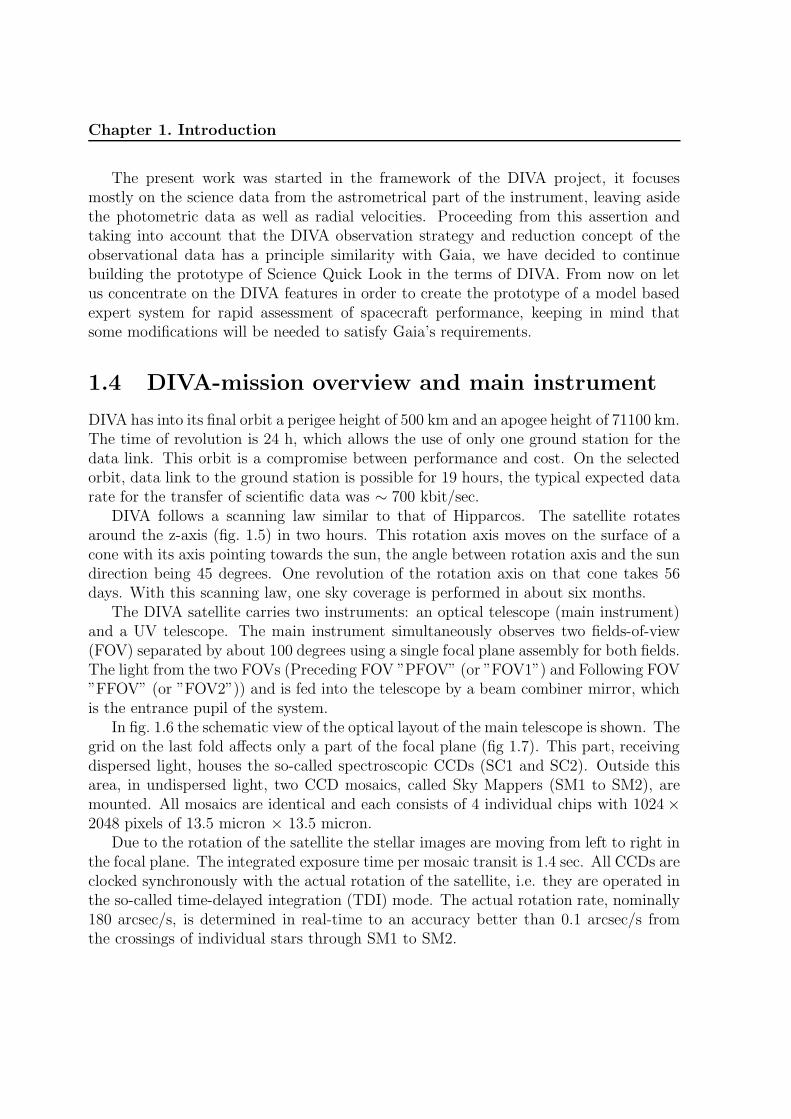
DIVA follows a scanning law similar to that of Hipparcos. The satellite rotatesaround the z-axis (fig. 1.5) in two hours. This rotation axis moves on the surface of acone with its axis pointing towards the sun, the angle between rotation axis and the sundirection being 45 degrees. One revolution of the rotation axis on that cone takes 56days. With this scanning law, one sky coverage is performed in about six months.

The DIVA satellite carries two instruments: an optical telescope (main instrument)and a UV telescope. The main instrument simultaneously observes two fields-of-view(FOV) separated by about 100 degrees using a single focal plane assembly for both fields.The light from the two FOVs (Preceding FOV ”PFOV” (or ”FOV1”) and Following FOV”FFOV” (or ”FOV2”)) and is fed into the telescope by a beam combiner mirror, whichis the entrance pupil of the system.

In fig. 1.6 the schematic view of the optical layout of the main telescope is shown. Thegrid on the last fold affects only a part of the focal plane (fig 1.7). This part, receivingdispersed light, houses the so-called spectroscopic CCDs (SC1 and SC2). Outside thisarea, in undispersed light, two CCD mosaics, called Sky Mappers (SM1 to SM2), aremounted. All mosaics are identical and each consists of 4 individual chips with 1024×2048 pixels of 13.5 micron × 13.5 micron.

Due to the rotation of the satellite the stellar images are moving from left to right inthe focal plane. The integrated exposure time per mosaic transit is 1.4 sec. All CCDs areclocked synchronously with the actual rotation of the satellite, i.e. they are operated inthe so-called time-delayed integration (TDI) mode. The actual rotation rate, nominally180 arcsec/s, is determined in real-time to an accuracy better than 0.1 arcsec/s fromthe crossings of individual stars through SM1 to SM2.

DR

AFT


Figure 1.5: DIVA scanning law

Figure 1.6: The schematic view of the optical layout of the main DIVA telescope.

DRAFT

Chapte

r1.

Intro

ductio

nmotion of starsSky mapper CCD mosaics

effective pixels1 * 4 physical pixels

on−chip binning

~ 0.025 square deg

~ 140 mm * 14 mm

µ 1 * 4 physical pixels

µ

~ 1800" * 180"

effective pixels

each mosaic

non−dispersed field dispersed field

4 * 1024 * 2048 pixels

Spectroscopic CCD mosaics

4 * 1024 * 2048 pixels

t = 1.41 sec

w = 13.5 m = 248 masw ~ 1.38 ms at 180"/sh = 54 m = 994 mas

34 a

rcm

in =

110

mm SM

1

SM2

SC1

SC2

optical axis

SM3

cold

redu

ndan

t

f = 11.2 m

Figure 1.7: The DIVA focal plane assembly: the main instrument uses a configuration of four identical CCD mosaics eachconsisting of 4 1k×2k CCDs, a 5th one (SM3) being added as cold redundant device.

DR

AFT


After detection in SM1 the on-board software shall predict windows surrounding thestars in the continuous pixel stream of the CCDs in the SM2 and in dispersed field.Only these predicted windows around the stars in the SM2, SC1, SC2 along with thedetected windows in SM1 will be transmitted to the ground.

In scan direction the full width of the central ”Airy” fringe in the both the SMs andthe SCs is about 1.4 arcsec at a central wavelength of 750 nm. In cross-scan direction itis 2 times larger. Therefore and because the main astrometric measurements are donealong scan a four times larger pixel size in this direction is used. In the DIVA concept,this is achieved via an on-chip binning of four pixels in cross-scan direction. So, read-outnoise as well as on-board data rates are reduced.

Attitude control is performed using a conventional cold-gas system. The analysis ofthe perturbations yielded that attitude maneuvers to keep the satellite on its scanninglaw are only needed at intervals larger than 10 min. Real-time attitude determinationwill ensure the knowledge of the attitude in all three axes to 10′′. During routine phasesthe use of the Sky Mapper CCDs will provide the attitude with an accuracy of betterthan 1′′.

The DIVA CCDs produce a pixel data stream that is much too big to be telemeteredto the ground entirely. The DIVA observation strategy is an astronomically motivatedprocedure for selecting specific parts of that raw CCD pixel data stream for inclusioninto the telemetry data stream sent to the ground. It is based on the fact that most ofDIVA’s raw CCD data cover almost empty, dark sky.

The essence of the idea [12] is to send only the so-called windows to the ground, smallsections cut out of the bulk data stream, which are centered on detected or predictedlocations of celestial objects. In our study we use a realistic model observation strategy(presented in [12]) which we discuss in the chapter 4.

1.5 Motivation for rapid assessment of payload and

spacecraft health in the framework of an astrom-

etry mission. Science Quick Look.

The spacecraft health management is a specific task of mission operations that has beenenhanced through the use of automation technologies. Through careful deploymentwithin the overall mission architecture, automation can augment or replace human de-cision making in order to increase reaction speeds, reduce errors and mitigate cognitiveoverload, enhance safety, lower costs, focus analysis and free human reasoning for strate-gic task [46]. Therefore, this automation requires high levels of robustness.

The space industry uses ground based monitoring software to analyze spacecrafthelth and detect faults. For the DIVA mission this monitoring will be performed in theframework of the Quick Look (QL) task. The QL software will help human operators totake care of the housekeeping of the satellite (bus and instrument) and attitude control

DR

AFT


system and prepares telecommanding if necessary. It is performed in real-time or inquasi real-time at the Space Operations Center3, using only so-called housekeeping data(HK).

However, the DIVA(Gaia) mission differs from typical astronomical space missionsin a way that the health of the science data can neither be judged nor guaranteed bymeans of diagnostics based only on HK data and attitude control system (ACS) data.It is mandatory to analyse also the science data. The term science data is used as acollective term for the bulk science data resulting from the instruments (SM-, SC-CCDsdata etc.).

For this reason a sophisticated daily diagnostics (First Look, FL) of the state of thesatellite is required to judge the level of precision of the stellar, attitude and instrumentparameters and to achieve its targeted level. The FL is the in-depth scientific assessmentof the quality of all observations within about 24 hours after its reception. It is based onthe complicated procedure called First Look preprocessing (or more known as a Great-Circle reduction from Hipparcos) that provides an one-dimensional, self-consistent andsimultaneous solution of the attitude, the instrument calibration and celestial source pa-rameters. For this purpose FL needs to treat all science data that can be only performedat the Data Center with its computer resources.

However, it is reasonable to process the science data for a quick discovery of delicatechanges in the spacecraft and performance at the same location where the QL task isexecuted, i.e. at the ground station and also in the quasi-real time constraints.

To do this we propose to develop a Science Quick Look (ScQL) monitoring, thatwill comprise the activities concerning science data health and alerts the operator whenproblems occur. Figure 1.8 depicts the scheme of the daily diagnostic with relationsbetween the Space Operations Center and the Data Center . The ScQL will performthe preliminary scientific assessment of the instrument and proper astrometric workingof the spacecraft at the (coarse) level of precision attainable at this stage. It shouldrun in quasi real-time at the space operations center using scientific data as well as HKdata.

1.6 The Goal of Ph.D. Thesis

The general goal of this research is to find ways to assist the operator-astronomer at spaceoperations center with the complex problem of rapid assessment of the astrometricalsatellite by

P helping them to deduce the changes of the state of the system from thescience data, producing statistics and diagnostics,

P providing expert advice on possible explanations of the problems.

3Space Operations Center = Ground Station (e.g. GSOC – German Space Operations Center,Oberpfaffenhofen).

DR

AFT


In particular, the focus of this study is on creating a prototype of the Science Quick Lookmonitoring software that should perform an initial science monitoring and diagnosticsusing the astrometrical science data in quasi real-time constraints. The ScQL is asimplified version of the First Look, and intended to immediately react on obviousdeviations from what is expected for the science data in order to safe an observationtime.

Data base

Satellite

Raw telemetry

Uncompression, formatting, etc.

Quick Look

House keeping data Science data

House keeping data

Science Quick Look

Initial data treatment

ScQL diagnostics QL diagnostics

Science data (attitude stars)

Telecomand

data flow

reports

commands

Initial data treatment

First Look Prepocessing (GCR)

Science data (all stars)

First Look

further data

reduction

FL diagnostics

Figure 1.8: The large scale interface between the ground segment (GS) and data center(DC) concerning Quick Look, Science Quick Look and First Look.

1.7 Guide to the Dissertation

The dissertation is organized into 7 chapters. This first chapter has introduced the astro-metrical spacecraft domain and its specific problem of the satellite health management.It is giving an overview of the astrometry and space astrometry missions such as Hippar-

DR

AFT


cos, DIVA and Gaia. The problems of monitoring of an astrometrical scanning satelliteare described and we reported about the motivation and goal of this investigation. Therest of the thesis is organized as follows:

2 Chapter 2 introduces the monitoring for dynamical systems, its objectives andtypical architecture. We then discuss different artificial intelligence techniques forthe monitoring and diagnosis task, focusing on the possible appropriate approachesfor the task of the Science Quick Look. In particular, we describe the traditionalsymptom-based systems such as a ruled-based system, fault dictionaries, decisiontrees and a case-based system and a new type of a diagnosis system with the so-called model-based reasoning, that relies on principle knowledge of the domain.We present the main components of model-based diagnosis systems, and thengeneralize the results of our study from literature about the modern state of themodel-based concept.

2 In chapter 3 we describe the conceptual design of the Science Quick Look mon-itoring. We introduce the design of the Science Quick Look, starting from set-ting up its monitoring requirements to the diagnostic solution. We introduce ourmodel-based approach with three functionally different parts of the ScQL system.We proceed from general to specific, exposing the main features of the monitoringsystem for a scanning satellite. We define a fault notion and discuss a resid-ual structure for correct alarm residual evaluation in the framework of our ScQLmonitoring.

2 The monitoring and the diagnosis are both based on a model for DIVA observationswhich is very complicated in the case of the scanning astrometry spacecraft. Tobuild the complete model of the observations is extremely challenging task. Thefirst step into this direction is the model that is explicitly implemented in the startransit simulator presented in chapter 4. In the framework of this simulator wedefine important components (sub-models) of our model, introduce and describeimportant entities and notions related to the sky and instrument that will beapplied to the whole system.

2 In chapter 5 we describe the design of the monitoring proper and the diagnos-tic parts of the ScQL in detail. The landscape of the environments for a typicalDIVA-application are discussed and the concept of mixed-language programmingis presented. The latter is used in order to build a rather flexible and databasecompatible ScQL monitoring software. Also the structure of the Visualizer isgiven, that is applied for the ScQL monitoring proper to provide a complex wid-get tool and display the pre-processed (and/or simulated) science data, statisticsand estimated parameters. Next, the statistics itself and estimated parametersat various levels of aggregation as well as the time-varying thresholds for alarms

DR

AFT


are described. Using these estimated parameters, detected by the ScQL monitor-ing proper, we introduce an initial list of possible explanations of the detectedproblems in the section dedicated to ScQL diagnosis. We emphasize that some ofthe presented faults can not be detected and uniquely identified by our diagnosisengine; in these cases a more detailed simulation is required. This should be thetask for future work.

2 Chapter 6 describes our evaluating procedure of the ScQL monitoring basedon the scenario – simulation – monitoring – matching cycle for its iterativelyevaluating and improving of the system. It allows to watch and validate thereaction of the ScQL monitoring. The science data with nominal parametersare simulated to derive computational solutions for a fault-free behavior of theinstrument. The number of fault scenarios are shown as examples of the ScQLprototype evaluation.

2 Chapter 7 lists accomplishments, practical considerations, limitations and out-look of this work.

DR

AFT


DR

AFT

Chapter 2

Monitoring systems

A year spent in artificial intelligence is enough to make one believe in God.

– Linux fortune program.

2.1 Monitoring and alarms

Any physical system evolves with time, either due to its own dynamics or under theimpact of external actions or events. Informally, monitoring a dynamic system canbe viewed as performed by a high level module which continuously keeps track of thesystem, analyses all the situations encountered, communicates with human operatorsand suggests decisions to be taken in case of malfunction. There is very little consensusas to the architecture of the ideal monitoring system. In general, it consists of severalcooperating modules (see figure 2.1):

• a detection module gathers elementary information (from raw data) and decideswhether the evolution of the process is normal, if not an alarm is generated;

• a diagnosis module, responsible for one or more of the following tasks:

– identifying characteristic situations;

– localizing the faulty components responsible for the situation;

– determing the primary causes of the abnormalities detected;

• a decision module which determines the actions which can be undertaken toreach the objective or bring back the process into normal conditions.

These modules rely on a knowledge base which contains:

• a library of detailed behavioral models of the physical system, under normal op-erating conditions and, when possible, in the presence of failures or in degradedmodes;

17

DR

AFT

Chapter 2. Monitoring systems

• the objectives to be met by the system, possibly together with plans of actionsboth in normal and in abnormal conditions,

• a description or several descriptions on various levels of the present state of thesystem, summarizing recent observations or expressing these in a language whichcan be understood by the operator.

System

Alarms

SEE

Faults

INTERPRET

Proposed Actions

DECIDE

Data/Signals

Signal Detection and Alarm Generation

DIAGNOSIS

A l a

r m D

e t e

c t i o

n a n

d I d

e n t

i f i c a

t i o n

L o c a

l i z a

t i o n

D i a

g n o

s t i c

Alarms Faults Decision-Support

Decision

I n s

t r u

m e

n t s ,

S

e n s

o r s

A c

t u a

t o r s

DETECTION DECISION

Figure 2.1: Typical architecture of a monitoring system.

The monitoring heavily relies on alarms, which rely in turn on sensor values, on theobservations related to the environment, etc. In fact, the concept of ”alarm” can varyfrom one application to another, which complicates the understanding and expression ofthe results. In [16] the definition of ”alarm” is suggested to be adopted, after analyzingtogether several applications in various sectors such as nuclear power systems, telecom-munication networks, etc.). This definition is based on the notion of ”event” which wedefine first followed by the one of an alarm:

- An event is a piece of information extracted from continuous or discrete signals(significant variations in a message emitted by the system) or extracted from dataabout the context (observational data, observations related to the environment,etc.).

- An alarm is a discrete indicator emitted by the monitoring system on the basis ofevents; it is intended to trigger a human or automated reaction.

DR

AFT

Chapter 2. Monitoring systems 19

Alarms can be determined either directly by a physical mechanism following simpleevent detection or by calculation, comparing the observation signal to a reference one.This gives rise to the following problems:

• What should the reference be?

• Should the signal be processed? How many values should be compared?

• What means of comparison should be adopted?

Alarms are mostly intended for the operator and they are processed on-line so thatthe operating conditions remain as close as possible to ideal ones, allowing for thevariability of input data and the natural evolution of the processes.

The purpose of monitoring is thus supervisory control and therefore the interpreta-tion must be done in real- or quasi real-time. In this case, when the operator controlsthe final decisions to be undertaken, an important issue is to avoid the ”cognitive over-load” problem characterized by a flood of data, some (or even most) of each beingredundant. The aim is hence to ”intelligently” organize the information supplied to theoperator. Whenever it is possible that decisions are taken with no human interventionand whenever it is important react quickly, interpretation of alarms may as well aim atautomatically appropriate reactions to the evolution observed on the system.

Automated interpretation of alarms may have one of several objectives: either todetermine the causes of a malfunction and provide explanations to the operator or topredict future behavior of the system so as to assess the degree of emergency of asituation, or to react automatically (by commands and/or physical mechanisms). De-termination of causes is similar to the overall process of diagnosis, and therefore calls forvarious techniques in the field. Among the possible causes, one can distinguish internalfaults related to equipment faults and external faults corresponding to input data thatare outside the acceptable range. Usually, it is necessary to provide explanations, andtherefore to describe explicitly some underlying implicit causal relations.

2.2 Artificial intelligence techniques for monitoring.

Related work.

There is a vast amount of work published on the subjects of monitoring and diagnosis– too much to cover adequately in this section. Our objective here is to focus on themost relevant approaches that have been considered (and influenced) in the process ofthe design of the Science Quick Look.

2.2.1 Symptom-based approaches

The idea of exploiting knowledge of causes for the purpose of diagnosis is quite natural.A dysfunction can be described in a simply way by relations associating its original

DR

AFT


causes (component failures, etc.) to observable manifestations, or symptoms. Having atheory which models this kind of relations, the diagnostic problem consists in using thetheory to seek satisfactory explanations of the observed symptoms.

Much of the literature on monitoring and diagnosis describes artificial intelligencemethods of associational inference that relate symptoms directly to faults. This encom-passes representations based on rules, decision trees, fault dictionaries, and the mostrecent case-based reasoning solving technique. Each of these methods has proven worthin various diagnostic settings, but at the same time they have several limitations.

Rule-based systems

Traditional rule-based systems have been built by accumulating the experience of theexpert in the the form of empirical associations – rules that associate symptoms withunderlying faults (see, for example, [28, 21, 5]). The problem-solving strategy may beeither forward-chaining (data-driven) or backward-chaining (goal-driven) or a combina-tional of both. The data-driven approach is most appropriate for the task of monitoring,where it is important to respond to new readings and alarms, combining multiple piecesof evidence to assess the severity of a problem and provide the operator with its inter-pretation. The goal-driven approach is most often used in diagnosis where the goal isa diagnostic conclusion and the rules, through backward-chaining, seek supporting evi-dence for various intermediate and final conclusions. Sometimes the logical processingfor a problem requires a combination of backward- and forward-chaining, called oppor-tunistic strategy [5]. It uses forward chaining to draw conclusions from existing dataand backward chaining to find data that make it possible to generate.

The rule-based approach became popular, because it permitted easy constructionof expert systems by encoding heuristic knowledge in the form of if-then and when-

then rules. This technique permitted rather quick and impressive demonstrations ofdiagnostic capability and promised that diagnostic coverage could be increased justby adding more rules. The early diagnosis systems, such as MYCIN in [20], used theheuristic knowledge for making diagnoses. However, several limitations became apparentas rule-based systems were applied to increasingly large and complex systems:

• The task of knowledge engineering (i.e., extracting experienced knowledge fromexperts and representing it in an appropriate form) is widely acknowledged tobe the bottleneck in the building of new expert systems. The representation ofthe heuristics included both domain and control knowledge – a mix that becomesunmanageable when the knowledge base becomes large and necessary to revise.As the system under study becomes larger and therefore more complex, the taskof knowledge engineering grows too.

• There is no guarantee that two faults (or more) that are individually diagnosablewill not interact in ways that mask any or all of the symptoms. A rule-based

DR

AFT


system may be validated on a set of test cases but still have important gaps in itsknowledge base.

• Rule-based systems have no (or very little) predictive power. They cannot showwhat will happen if a fault is left unrepaired. Similarly, it is difficult to expressand reason about temporal information, such as the evolution of symptoms of afault.

• Small changes in the design of the system may necessitate revisions in a large partof the rule-base. So, once implemented, the systems are difficult to maintain.

Decision Trees

Decision trees provide a guide to diagnosis in a way that they write down the sequenceof tests leading to a diagnostic conclusion. A decision tree is a hierarchically arrangedsemantic network. It is composed of nodes representing goals and links that representdecisions or outcomes. A major advantage of a decision tree, therefore, is to verify logicgraphically in problems involving complex situations that result in a limited number ofactions.

Decision trees are typically built manually by engineers using detailed knowledge ofthe system’s design and its known failure modes. Such decision trees may contain notonly diagnostic steps but also recommended control actions to ensure system safety.

As Davis and Hamscher [21] point out, the simplicity and efficiency that is a strengthof decision trees is also an important weakness: they are a way of writing down adiagnostic strategy, but offer no indication of the knowledge used to justify that strategy.Decision trees thus lack ”transparency” and are therefore difficult to update (smallchanges to the mechanism may require a major restructuring of the tree). Like othermethods, decision trees have no predictive power to reveal the propagating effects of afault.

Fault dictionaries

A fault dictionary is a list of symptom/fault pairs, indexed by symptom. The dictio-nary of the monitored system must be built for every kind and combination of faultsanticipated. To do this a description of how the entire system would behave if specificcomponents were broken in a specific way should be generated. This generation can bedone by the simulation of the monitored process. The result is a list of fault/symptompairs, which is then inverted to form a dictionary of symptom/fault pairs. An examplesof this technique can be found in [63].

To an extent, fault dictionaries are forerunners of a model-based approach (see below)and overcome some of the limitations associated with rule-based systems, namely: thedictionary does not depend on experience, it can expose the effects of interacting faults,it can be regenerated mechanically if the design changes, and it is likely to cover more

DR

AFT


fault scenarios because of its systematic (though not exhaustive) treatment of the kindsand combinations of faults.

The idea behind fault dictionaries – systematic generation of symptom/fault associ-ations – is good, but the technique has some practical limitations:

• In a single entry of the dictionary the symptoms are essentially a predicate on asnapshot of the system. This kind of matching fails to exploit temporal continuityin the evolving manifestations of a fault (this approach can be made vital bygetting the right hypothesis and refuting incorrect hypotheses).

• Only the most likely failure modes of each component are considered, and thereforethe combination of faults is also severely limited.

Case-Based Reasoning

A relatively recent problem solving technique is the so-called case-based reasoning(CBR). It is attracting increasing attention because it seems to directly address theproblems outlined above.

A CBR technique, the origin of which is widely held by the work [59], solves newproblems by adapting previously successful solutions to similar problems. It does notrequire an explicit domain model and so elicitation becomes a task of gathering casehistories; the experience does not need to be completely understood, only recorded, theimplementation is reduced to identifying significant features that describe a case; CBRsystems can learn by acquiring new knowledge as cases, thus making maintenance easier.This technique in the case of monitoring of the behavior of complex physical systems,however, has also some disadvantages, including:

• It is necessary to build a library of cases before the system will be useful.

• Some values may be more significant in some contexts than others. Unless theuser specifies the particular importance of those values, they will be treated withthe same importance as the rest of the values.

• Cases require interpretation, as a CBR reasoner does not necessarily provide the”correct” solution for a problem; it merely provides suggestions of possible solu-tions.

2.2.2 Model-Based Reasoning

In response to the problems in symptom-based systems, a new type of diagnosis systemwas developed that did not include empirical knowledge about symptoms and diagnoses,but relied on principle knowledge of the domain. A diagnosis system of this type is calledmodel-based, because it has a model of the diagnosis object, which describes the ob-ject (see, for example, [23] and [18]). ”The model-based reasoning (MBR) process itself

DR

AFT


can be viewed as the symbolic processing of an explicit representation of the internalworkings of a system in order to predict, simulate, and/or explain the resulting behaviorof the system from the structure, causality, function and behavior of its components”[69]. In other words, model based diagnostic reasoning is an interaction between pre-diction and observation [21]. Thus, the first step in MBR is the building of an accuraterepresentation (model) of the system that you want to be able to reason about. Oncethere is a complete model and an algorithm which correctly reproduces the relation-ships and behavior of the system, one can get complete, precise solutions based on a setof inputs. This technique allows both simulating the behavior and making inferencesabout the values of unmeasured variables. By matching versus predictions rather thansymptomatic patterns, model-based diagnosis also avoids combinatoric problems.

The principles of model-based diagnosis are well understood. The diversity of work inthis field owes largely to the various types of models, representing many different degreesof abstraction. Our coverage of this field within this framework therefore attempts onlyto be representative rather than exhaustive.

Modeling for Troubleshooting (Davis & Hamscher)

Model-based diagnosis, as commonly described in the AI community [21], requires mod-els of structure and behavior of the system/mechanism under study. One might assumethat an adequate structural model is simply a complete hierarchical description of sub-systems and components, and that an adequate behavioral model is a detailed simulationmodel that predicts all the time-varying events/changes in the mechanism. While suchmodels do support model-based diagnosis, they are also part of the problem. As Ham-scher emphasizes, the important thing about developing a model for troubleshooting isnot that it uses abstractions to deal with complexity (any representation does that), butthat it embodies structural and behavioral abstractions appropriate to troubleshooting.

What sort of abstractions are helpful in troubleshooting? Hamscher identifies eightprinciples to guide a knowledge engineer in constructing a model that makes trou-bleshooting feasible. Although Hamscher’s research concerns digital circuits (a form ofdiscrete-event dynamic systems), the principles are general enough to be applied, inmost cases, to the continuous-variable dynamic systems.

These principles separate into three categories: behavior, structure, and failures.We show the eight principles here to give interested readers a fuller understanding ofHamscher’s insights, and we recommend his article for explanations of each.

Modeling of Behavior

– The behavior of components should be represented in terms of features thatare easy for the troubleshooter to observe.

– The behavior of components should be represented in terms that are sta-ble over long periods of time or that summarize much activity into a single

DR

AFT


parameter. This is easiest for a component for which changes on its inputsalways result in changes on its outputs.

– A temporally coarse behavior description that only covers part of the behaviorof a component is better than not covering any at all.

– A sequential circuit should be encapsulated into a single component to enablethe description of its behavior in a temporally coarse way.

Modeling of Structure

– Components in the representation of the physical organization of the circuitshould correspond to the possible repairs of the actual device.

– Components in the representation of the functional organization of the circuitshould facilitate behavioral abstraction.

Modeling of Failures

– An explicit representation of a given component failure mode should be usedif the underlying failure has high likelihood.

– An explicit representation of a given component failure mode should be usedif the resulting misbehavior is drastically simpler than the normal behaviorof the component.

Qualitative models

The behavior of a physical system can be described by the exact quantitative values ofits variables at each time instant. Qualitative physics is an alternative physics in whichthe insight concept of the system is defined within a far simpler qualitative basis, butnevertheless formal [22].

Qualitative physics provides a broad integrated and formal account of behavior –an account rich enough to enable intelligent systems to perform tasks such as diag-nosis, analysis, explanation and even simulation. Fig. 2.2 illustrates the approach ofqualitative physics contrasted with conventional(quantitative) physics. Both start bymodeling physical situations, both end with a qualitative common sense description ofthe behavior. The first step in the conventional approach is to formulate and solve thedifferential equation to obtain a solution. The second step is to interpret this solutionto obtain common sense description of the behavior. The qualitative analysis begins byformulating qualitative differential equations and then solves these. The result is a sim-ilar common sense description of the behavior and causal explanation for that behaviorwhich is obtained ”more simply”.

Unlike quantitative variables, qualitative variables can only take one of a small num-ber of values. Each qualitative value corresponds to some interval on line of the real

DR

AFT


Modelling Solve

Modelling

Physical situation

Differential equations

Qualitative differential equations

Solve Analytical solution

Common sense description

Figure 2.2: Comparison of qualitative and quantitative approaches.

numbers. Landmark values demarcate the boundaries between qualitatively distinguish-able intervals. The most common landmark is zero, in which case three important qual-itative values are positive, negative, and zero or, for a derivative, whether a quantity isincreasing, decreasing, or constant.

The most commonly used qualitative simulator QSIM [48], that has been used asthe core of a monitoring system called MIMIC [25], allows for implementing this typeof models. The QSIM-style constraint model describes the physical device as a set ofcomponents. A set of QSIM qualitative states characterizes the device’s observed faultybehavior. Two phases can be distinguished in MIMIC: monitoring and diagnosis, bothof which call QSIM. The concepts of monitoring, diagnosis and simulation are associatedin a cycle of hypothesis/model building/simulation/comparison. MIMIC uses a libraryof qualitative models including one model of normal and failure models. The fault modelwhose predicted behavior matches the faulty behavior then determines the set of faultsin the device.

The approach based on qualitative simulation is well suited to the needs of monitoringtasks with the a high-level of abstraction where the qualitative formalisms are particularuseful in representing imprecise, uncertain or incomplete knowledge.

Inc-Diagnose

In 1987 Reiter proposed a formal theory of diagnosis from first principles that reasonsfrom system descriptions and observations of system behavior [55]. The algorithm com-putes all minimal diagnoses of a device, including multiple-fault diagnoses. In contrastto an abductive approach to diagnosis in which the hypothesized faults must imply orexplain the symptoms, Reiter’s theory requires only that a diagnosis be consistent withthe system description and observations; no notion of causality is needed. However, thetheory was applied only to diagnosis of digital circuits, which are representative only ofphysical devices having discrete, persistent states. Reiter’s theory is not in conflict with

DR

AFT


the well-known model-based diagnosis work of researchers such as Davis & Hamscher[21] and deKleer & Williams [23]; rather, it gives a stronger theoretical foundation forthat work.

In 1990 Ng [67] extended Reiter’s algorithm to diagnose dynamic continuous devicesof the kind modeled by QSIM. Since QSIM represents continuous behavior as a finitenumber of discrete qualitative states, it allows the diagnosis problem to be transformedfrom a continuous one to a discrete one. Ng’s algorithm, named Inc-Diagnose, makesReiter’s approach incremental in that it permits measurement-taking at different times,intermixed with hypothesis generation. Like Reiter’s approach, Inc-Diagnose can diag-nose multiple faults using only a correct model of the device; Inc-Diagnose does not usefault models (see MIMIC) and it cannot predict the effects of faults.

2.2.3 Fault detection and isolation

The main objective of the fault detection and isolation (FDI) research area, widelyaddressed from several points of view since the early ’80s, is to study methodologiesfor identifying and exactly characterizing possible incipient faults arising in a plant. Ascommonly referred to in the literature on this topic (see [17]), the term fault detectionis used to describe the problem of making a binary decision either that something hasgone wrong or that everything is fine. This is usually achieved designing a dynamicalsystem (usually referred to as a filter) which by processing input/output data is able todetect the presence of an incipient fault and eventually to precisely isolate it generatingthe so-called residual signals. There are different ways which can be adopted to detectand isolate the fault. A common way, in some industrial applications, is to use hardwareredundancy, which consists of comparing the outputs of identical hardware and performconsistence cross checks. As it can be easily realized, this approach is not always feasiblein practice due to an economical impact. A solution of this kind may have a cost of theanother whole system.

Using a different approach, known in FDI literature as analytical redundancy, theFDI task can be accomplished using analytical and functional information about thesystem using a mathematical model of the system (model-based FDI). An analyticalredundancy relation (ARR) expresses a constraint among possible observations thatholds when the system is working correctly. The FDI structure is the minimal set ofcomponents whose models have to be satisfied for the ARR to be satisfied. If some ARRrelation does not hold, then the system is faulted and the degree to which the relationsare violated are the residuals.

2.3 Summary

The primary goal of a diagnostic system is to detect anomalous system behavior andthen to isolate the cause for such a behavior. One thing is very clear from a study

DR

AFT


of the literature – there is no universal method, which could be able to cope with allkinds of systems and all possible faults. Therefore it is important to set clear diagnos-tic requirements beforehand, i.e. types of faults, performance attributes, and availableprocess knowledge should be clearly identified. A model-based approach seems to bemost appropriate when tackling problems in monitoring and control of a complex systemsuch as spacecraft when the description from the first principles of the domain is morepreferable. The basic concept of this approach is to use a model to predict expected be-havior, and then using discrepancies between predictions and observations as diagnosticclues. This approach is rather natural for solving the problems in science, as it is thescientist’s aim to investigate and describe the structures and mechanisms underlyingphysical processes.

There are two classes of model-based approaches:

• In the first class quantitative models are used. These approaches are based on thephilosophy that a fault changes the physical parameters and hence the model of thesupervised system. These methods make use of theoretical tools such as parameterestimation techniques, state estimation techniques and parity space concepts. Inthis approach the need for an a priori knowledge about the relationships betweenfaults and changes in model parameters and states is a key point.

• The second approach is based on the use of qualitative reasoning and modeling,that are used to predict the behavior of the system in nominal conditions and indifferent faulty condition and the isolation of the fault is performed comparing thepredicted and the actual behavior.

MBD Engine

Component Model Library

Diagnosis

Observations

Structural

Description

Figure 2.3: Basic perspective of MBD [24].

The concept of model-based approach, called model-based diagnosis (MBD), hasevolved in two separate communities with their own terminologies and conventions:

DR

AFT


the model-based reasoning (MBR), a specialty within the AI community and the faultdetection & isolation (FDI), a specialty within engineering community. Nowadays, thereis an attempt to present the fundamental concepts of MBD in one consistent terminologyand thus to make the field much more accessible. The authors of [24] illustrates the basicproperties of MBD, discuss the differences in formal definitions, conflict treatmentsand basic perspective of MBD. In [24] is noted that the main characteristics of theMBD approach are an emphasis on general diagnostic reasoning engine that perform avariety diagnostic tasks, and inference of a system’s global behavior from the automaticcombination of local models of its components. This is illustrated in figure 2.3 wherethe component library used by an MBD engine describes the laws which govern thebehavior of the components.

The model-based diagnosis is an active area of artificial intelligence research andit has been approved as a useful technique to monitor and automatically diagnose ofspacecraft failures with a large number of components. In [14] and [70] model-basedsystems have been made scalable enough to be applied to systems with up to tens ofthousands of components.

DR

AFT

Chapter 3

From Requirements to DiagnosticSolutions

Monitoring and diagnostic system design starts with setting up diagnostic requirementsand process knowledge.

The objective of this chapter is to set up the requirements of the monitoring systemin sufficient detail to enable a rational design. We proceed from general to specific,starting here with the high level-architecture of the ScQL monitoring system and thenelaborating on its components in the following chapters.

3.1 Requirements of the Science Quick Look (ScQL)

As in any other engineering design, we start the design of ScQL monitoring systemwith setting up its diagnostic requirements. The core of every diagnostic solution is thechoice of a suitable process model (see fig. 3.1). This is conditioned by available processknowledge, given measurements, and is closely related to the requirements. The levelof abstraction and accuracy of the model has to be chosen in such a way that givenrequirements are fulfilled.

As mentioned, a monitoring of various kinds is required to continuously check thecorrect operation of all aspects of the instrument, both as individual components andas a complete system. The aims of the monitoring may be generally classified by thefollowing main requirements:

(1) Monitoring of the on-board instrument hardware,

(2) Monitoring of the on-board instrument software.

This monitoring is an important part of the whole daily data reduction process (figs. 3.2and 1.8) and represents an indirect control of the work of the on-board hardware andsoftware. It is based on the analysis of the observations (science data) and treated inquasi-real time on ground at the space operation center.

29

DR

AFT

Chapter 3. From Requirements to Diagnostic Solutions

Knowledge

MODEL

Observations

Requirements

Model-based system

DESIGN

Figure 3.1: A model-based system design.

Observations

SKY

INSTRUMENT

Hardware (H/W) Software(S/W)

Data Reduction

Quick Look (QL): House Keeping Data (2-8 h)

M o

n i t o

r i n g

Science Quick Look (ScQL): Attitude Stars (2-8 h)

First Look (FL): All stars (24 h)

Science Data

House Keeping Data

Figure 3.2: Overall scheme of the daily monitoring and diagnosis.

DR

AFT

Chapter 3. From Requirements to Diagnostic Solutions 31

Data sets for the ScQL

Before we start describing the main requirements to the system in details, let us shortlypresent the data sets for the ScQL monitoring system. These data contain

I. The so-called windows (containing star images) are the central observationsresults produced by the main instrument. There is one window record per on-boarddetected or predicted star image, plus some special windows (sky background). Onaverage there will be about 100 windows(recors)/sec (for SM mosaics), but thisvaries between about 50 and 1500 windows(records)/sec, because the Milky Waysystem has a disk-like distribution of stars (i.e. our galactic disk has a higherdensity of stars compared to the halo).

II. Parts of the house keeping data: TDI timing, the values of supply voltages ofthe CCDs, the values of the thermal status of the CCDs.

III. Orbital parameters of the satellite.

IV. Attitude control system data: scan speed of the satellite, orientation of thesatellite, etc.

A detailed description of the ScQL data sets is presented in Appendix 8.2 and discussedfurther in Chapter 4.

(1) Monitoring of the on-board instrument hardware

It must be possible to verify whether the hardware of the main instrument of DIVA– instrument processing unit (IPU) – is functioning correctly. This encompasses theoptics of the main instrument and detectors with its light sensitive area (CCD mosaic,see figure 1.7) and supply voltages of CCD ADU chains1.

(2) Monitoring of the instrument on-board software

It must be achieved to verify that the algorithms of on-board software of DIVA IPU isfunctioning correctly. Some of the following algorithms are still under construction andshould be considered as preliminary ones for the tasks of the ScQL, however, they areenough developed to be included and described for the tasks of the ScQL.

• Detection algorithm on SM1 (see fig.1.7). The on-board image detectionprocess performed by the instrument of the satellite constitutes a crucial elementfor the success of the astrometrical mission. The on-board detection ultimatelydefines DIVA’s sky survey – its completeness, its brightness limits and its biases.The primary output of the image detection software is a list of star-like images that

1ADU – Analog to Digital Unit that corresponds to a half of CCD chip area.

DR

AFT


are detected in the input data stream. In [7] the different criteria for the judgmentof the scientific performance of the image detection algorithm, to be used in theindustrial development of the satellite, are discussed. One of the possible simplealgorithms of the on-board detection for DIVA were described in [42, 41]. In [41]was applied a block-skipping method for acceleration of object detection.

• Centroiding algorithms. The on-board centroiding algorithm generates thecentroids for the objects (images) on SM1, the coordinates of the centroid (µcand κc) are the coordinates of the centroid in cross-scan and in scan directionscorrespondingly. There exist two types of centroiding algorithms that define thecentroids with a different precision. This precision of centroids is defined by the therequirements of the consecutive tasks such as the prediction algorithm, the attitudecontrol system, the rate of the star transit and TDI clock stroke adjustment.

– Coarse centroiding algorithm. This algorithm provides the centroidsof the detected object (image) on SM1 for the cutting of the window andprediction of the left-corner of the window on SM2 (there is no detection onSM2)2. In this case the mean error of the centroids should be ∆µc,κc ' 1pixel in both directions because one can only cut the window with an integernumber of the left-corner.

– Fine centroiding algorithm for attitude stars. This algorithm providesmore accurate centroids than the coarse centroiding algorithm for the objectswhich are identified as attitude stars. These centroids will be used furtherby the attitude control system for the following attitude determination, thestar transit rate and TDI clock stroke adjustment.

Note: There are several methods (see [34, 35, 36, 9]) to calculate the centroidssuch as numerical filters, moment methods, gaussian fits and profile fits (the lastone, based on the DIVA point spread function (PSF), is the most accurate methodto calculate the centroids).

• Prediction algorithm on SM2 (see fig.1.7). This algorithm takes the cen-troids of the objects from SM1 as input and predicts the location of the windowssurrounding the objects in the continuous pixel stream of the CCDs on SM2 andzero-order SC. The original algorithm, proposed in [12], was extended in [9] tomake it more appropriate for the on-board software logic.

• Window cutting algorithm. This algorithm cuts out a small section of the rawCCD pixel data stream, the so called window, surrounding the objects. Only thepredicted windows around the objects on SM2 & SC along with detected windowson SM1 are transfered to the ground.

2In fact, there is a very small pixel area on SM2 where the object detection should be performed.

DR

AFT


• Background determination algorithm. This algorithm determines the signallevel of the so-called ”empty sky”. The optimum way to do that in an astronomicalcontext uses a median of the signal over extended sky areas. However, it is notpossible to implement it in the on-board software, instead one will use groups offour consecutive pixels in a line to infer the background levels (see [9] for moredetails).

• TDI clock stroke rate adjustment algorithm. Due to the rotation of thesatellite the stellar image are moving from left to the right in the focal plane.So, all CCDs should be clocked synchronously with the actual rotation of thesatellite. They are operated in time delay integration mode and therefore havean integrated exposure time per CCD transit equal to texp = 1.4 sec in nominalmode. The actual rotation rate, nominally ω = 180′′/sec, must be determined inreal time to an accuracy better than ∆ω ≤ 0.1′′/sec from the derived rate of thestar transit. If the shifting of the charge on the CCD does not match the actualrotation of the satellite, but this mismatch is not yet large enough to initiate thejet-firing, then a new TDI clock stroke rate must be determined which which issynchronized with scan-speed of the satellite. We propose two methods for theTDI clock adjustment from the star rate determination which can be used for theon-board TDI clock stroke rate adjustment and for on the ground control of thisprocess in the framework of the ScQL monitoring system as well.

• Attitude star catalogue handling. The attitude star catalogue consists ofreference stars, i.e. stars with known positions, magnitudes, proper motions andcolors. These stars play an important role in the on-board attitude determina-tion and TDI clock stroke adjustment. The complete algorithm for the on-boardattitude star handling is described in [6] in general, especially designed for as-tronomers. But one can use the approach of [9] with a more precise description ofeach step of the attitude star catalogue handling that includes:

– Creation of the working catalogue. It is constructed to reduce CPU timeduring observations and is prepared in the following steps:

∗ Calculation of the nominal scanning law attitude;

∗ Selection of all attitude stars for the next several rotation of the satellite;

∗ Computation of reference great-circle coordinates for all selected attitudestars;

∗ Transformation of the cartesian vectors into RGC longitude and latitude;

∗ Sorting stars along reference great-circle longitude.

– Identification of attitude stars. With the aid of the working catalogue theidentification of attitude star transits is performed according to the followingsteps. To reduce computational load further, only detected images whichare brighter than ≈ 12.5 magnitude are considered as possible candidates forattitude stars.

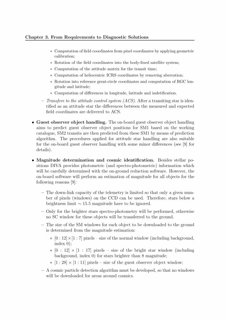
DR

AFT


∗ Computation of field coordinates from pixel coordinates by applying geometriccalibration;

∗ Rotation of the field coordinates into the body-fixed satellite system;

∗ Computation of the attitude matrix for the transit time;

∗ Computation of heliocentric ICRS coordinates by removing aberration;

∗ Rotation into reference great-circle coordinates and computation of RGC lon-gitude and latitude;

∗ Computation of differences in longitude, latitude and indetification.

– Transfere to the attitude control system (ACS). After a transiting star is iden-tified as an attitude star the differences between the measured and expectedfield coordinates are delivered to ACS.

• Guest observer object handling. The on-board guest observer object handlingaims to predict guest observer object positions for SM1 based on the workingcatalogue, SM2 transits are then predicted from these SM1 by means of predictionalgorithm. The procedures applied for attitude star handling are also suitablefor the on-board guest observer handling with some minor differences (see [9] fordetails).

• Magnitude determination and cosmic identification. Besides stellar po-sitions DIVA provides photometric (and spectro-photometric) information whichwill be carefully determined with the on-ground reduction software. However, theon-board software will perform an estimation of magnitude for all objects for thefollowing reasons [9]:

– The down-link capacity of the telemetry is limited so that only a given num-ber of pixels (windows) on the CCD can be used. Therefore, stars below abrightness limit ∼ 15.5 magnitude have to be ignored.

– Only for the brighter stars spectro-photometry will be performed, otherwiseno SC window for these objects will be transferred to the ground.

– The size of the SM windows for each object to be downloaded to the groundis determined from the magnitude estimation:

∗ [0 : 12]×[1 : 7] pixels – size of the normal window (including background,index 0);

∗ [0 : 12] × [1 : 17] pixels – size of the bright star window (includingbackground, index 0) for stars brighter than 8 magnitude;

∗ [1 : 28]× [1 : 11] pixels – size of the guest observer object window;

– A cosmic particle detection algorithm must be developed, so that no windowswill be downloaded for areas around cosmics.

DR

AFT


• Compression algorithm. As we discussed above, the data transmission rate ofDIVA satellite is ∼ 700 kbit/sec, therefore not allowing to download the wholeCCD frames to the ground station. So, one uses the strategy that permits totransfer only the parts of the CCD mosaics, windows, that contain the necessaryscientific data. However, even with this cutting the data rate could sometimesexceed the transmission rate. So, a simple loss-less data compression algorithmis desired in order to download as many scientific data as possible. For this pur-pose, in [9] a simple algorithm was proposed and tested. It allows to achieve thecompression rate of almost a factor of 2 and the coding is simple and fast, so atthe moment this algorithm is considered to be reasonable robust for the on-boarddata compression.

3.2 The design of the ScQL

A model-based approach for the ScQL

The task of the ScQL monitoring system is further complicated by the fact that thebehavior of individual components can evolve over time and, in some cases, changesare due to the activity of other components. Thus, alarms are not independent, i.e.some are merely the consequence of the others. The distinguishing feature of the ScQLmonitoring is to collect, analyse and interpret the science data, but not onlythe house keeping data. So, the analysis and interpretation of the science data is a clueto the fault detection of the components of the DIVA main instrument. The analysis ofthe DIVA instrument behavior can be viewed as an interaction between prediction andobservations of the science data. By matching the observations against predictions ratherthan symptomatic patterns, model-based technique provides the simulation mechanismto cover a very broad collection of possible faults and will allow therefore to make indirectinferences about the behavior of components of the DIVA instrument.

The diagnosis of the science data is thus based on the modeling of the behavior ofthe DIVA with its observing scanning strategy.

There is no other way to provide the ScQL monitoring with the predicted obser-vations (predicted science data) as to model them quantitatively. A purely qualitativemodel is absolutely inappropriate for this purpose because we have to keep the diagnos-tic accuracy and precision as high as possible to satisfy the observation requirements ofDIVA as described in [11]. However, it does not mean that we will not make simplifi-cations in our model for the science data simulation and therefore for the data analysisand diagnosis. The purely qualitative descriptions, applied usually for a qualitativesimulation, when the values of variables are described in terms of their relations witha finite set of symbolic landmark values. However, it can be augmented with semi-quantative knowledge in the form of real bounding intervals and real-valued functions.We will combine this semi-quantative approach, that helps us to describe the behavior

DR

AFT


of some components of the system considering only the high level of abstraction, andthe quantative model in order to derive the diagnostic ability of the ScQL monitoring.Therefore,

our approach is to combine all necessary pieces of knowledge fromdifferent abstraction levels in order to cover iteratively the task ofthe fault detection by the analysis and interpretation of the sciencedata in the framework of the ScQL monitoring.

Indeed, to keep the description of some complex components of the instrument at thehigh level of abstraction is rather reasonable at this stage of the project. It permits tocreate an extended skeleton of the ScQL monitoring and make the simulation traceablein spite of the lack of the detailed qualitative model of the behavior of these components.

Schematically, the whole process of our monitoring system can be represented bythree functionally different parts (see fig. 3.3):

ScQL monitoring process

SS => O

Generation of o bservations

O => S

Symptom generation

S => F

Symptom evaluation (Reasoning)

Star-Transit Simulator

Monitoring Proper Diagnosis

Figure 3.3: The ScQL monitoring parts: SS – Sky (Galaxy) & Satellite models, O –Observations, S – symptoms, F – faults.

P Star transit simulation is used as a core of the ScQL monitoring to modelthe behavior of the satellite and simulate the observations by the quantative andsemi-quantative model approach. It is described by the functional behavior of thesystem according to the chosen accuracy and abstraction level. This descriptionis based on the model of the Galaxy, the structure of the DIVA satellite and itsobservation strategy. The star transits simulator provides the ScQL monitoringwith astrometrical science data, i.e. with the data from the Sky Mapper CCDmosaics.

It is worth to mention that we consider the star (space object) as a point sourceon the sky and on CCDs, so we simulate the star transits in the form of suitablecoordinates, centroids (see chapter 4 for details), instead of pixel images. By thisapproach we can generate directly the image parameter set – the output from

DR

AFT


the initial data treatment (see on fig. 1.8) and avoid an explicit implementationof the first step of the scientific data reduction chain that consists of pixel dataprocessing.

P Monitoring proper estimates statistics and parameters from the observations(simulated science data) and generates the symptoms (residuals) via analyticalredundancy. The statistics and derived parameters are compared to their expec-tation values and if the findings differ significantly from the nominal ones, thesystem rises alarm flags and generates appropriate symptoms.

The monitoring proper performs updating the ”monitoring set” composed of thoseparameters and their tolerances which are appropriate for the present state of thesatellite.

P Diagnosis uses the symptoms, generated by the monitoring proper, to performtheir evaluation in order to debug the abnormal (fault) situations. We define thefault as any disturbance of the observations at the scientific level of the precision.So, this third parts gives the relation between the symptoms, that are representedthrough statistics and estimated parameters of the instrument and faulty statesof the system.

The monitoring and diagnosis are both based on the model that is explicitly implementedin the star transits simulator. The role of the monitoring and diagnosis task is to generateand evaluate the symptoms derived from the analysis of the generated dataflow and topresent this analysis to the operator to assist in interpreting it and diagnosis. Thealarms which indicate either dysfunction or significant events are produced in the quasi-real constraint, i.e. every 15 – 30 min a new set of alarms is generated. This discrete-timeconstraint allows us to leave aside the problems related to real-time monitoring systemswhen propagation times of events, alarms and transmission paths must be taken intoaccount. It is worth to mention that in our study we focus on the tracking anddiagnosis aspects of the ScQL monitoring system not on the advising aspect.So, we do not develop in this work a final advising system based on diagnostics. Thisshould be the task for future research.

Faults and residual generation

We defined above the fault as an unexpected (unpermitted) deviation of at least onecharacteristic property of a variable from an acceptable (nominal) behavior of the satel-lite. Therefore, the fault is a state that leads to a malfunction of the system. Thetime dependency of faults can be distinguished, as shown in figure 3.4, as abrupt faults(stepwise), incipient faults (drift like), intermittent faults. An abrupt fault appears asa quick increase in the observed symptoms, a sudden breakdown of the component, e.g.ADU chain. Incipient fault gradually develops as a function of time (slow degradationof components).

DR

AFT


Figure 3.4: Three typical classes of the time-dependency of faults: (a) abrupt fault, (b)incipient fault, (c) intermittent fault.

Detection of faults in ScQL is based on symptoms/residuals that are reflected thechanges of observable quantities from their normal behavior. Normally, the consistencycheck based on analytical redundancy (see Chapter 2) is achieved by comparing theavailable signals (known inputs and measurements) and a model of the system. A cross-check of these signals is carried out to detect faults. The resulting difference for onesignal is referred to as residual signal:

ri(t) = yi(t)− yi(i), i ∈ k,

where ri denotes the ith residual, yi the ith measured system output, yi the estimatedith system output and k the number of residuals. The goal is to generate structuredresiduals to meet monitoring and diagnosis requirements. More generally, the generationof residuals is performed by the estimation of the system measurements, output vectory, or of the system parameter vector θ. Then the estimates y and Θ are substractedfrom the real observations y and/or from the system parameters Θ. This leads to thefollowing residual vectors:

ry(t) = y(t)− y(t) or rΘ(t) = Θnom(t)− Θ(t)

This residual vector ry(t) is typical for the observer-based approach, whereas the rΘ(t)corresponds to the parameter estimation approach. Residuals are designed to be equalor converge to zero in the fault-free case (ri(t) ≈ 0) and deviate significantly from zero

DR

AFT


under occurrence of a fault (‖ri(t)‖ > ηi > 0, where ηi ∈

denotes a threshold). Hence,the residuals represent the fault effects.

In our monitoring system the parameter estimation approach of residual generation(based on different statistics of the science data) is chosen. As for the observer-basedapproach is concerned it may be apply to the house keeping data, the residuals of whichmight be derived directly from the output of the satellite. But we will not consider thisin our study, and so in the following and in the rest of the thesis only the parameterestimation approach is considered in details.

Residual evaluation and residual structure

A successful residual-based approach requires an appropriate residual evaluation in orderto take the following decisions: 1. Is there any fault present?, and 2. If yes, which fault(s)is/are present. Especially the second decision is depending on the fact whether onlysingle faults (one fault at a time) or also multiple (simultaneous) faults are considered.The problem of handling multiple faults lies in the fact that resulting faults effectscaused by single faults occur at the same time and hence, they might compensate eachother the might overlap in a way that either only one of them or a complete other faultis detected.

Therefore, it is important to obtain the correct residual structure for correct residualevaluation. The residuals should be generated in such a way that for each fault adifferent set of residuals is affected (i.e. the residuals deviate significantly from zero).For multiple faults it should furthermore be guaranteed that the overlapping of theresulting fault effects does not lead to the wrong decision, i.e. missed detection of afault or a wrong decision about which fault occurred.

A structured residual can be characterized by the following property: Any residualresponds only to a specific subset of faults, and to any fault only a specific subset ofresidual responds. Following [30] one can represent a set of p residuals in in two differentways:

• in a geometric way by considering the vector

r(t) = (r1(t)r2(t)...rp(t))T , where r(t) ∈ p.

• in a Boolean way by defining a fault code vector in the following way:

εi(t) =

1, if ‖ri(t)‖ ≥ ηi;

0, if ‖ri(t)‖ < ηi

⇒ ε(t) = (ε1(t)ε2(t)...εp(t))T

for i ∈ p and the thresholds ηi.

DR

AFT


Obviously, the fault code vector ε(t) provides the information whether the ith resid-ual ri(t) hits a defined threshold ηi or not. In the Boolean notation one can alsodefine a structure matrix Φ in the following way, when using the fault vector ν(t) =(ν1(t)ν2(t)...νk(t))

T :

r← Φν

where the jth column vector of Φ is defined as: Φj = ενj , where ενj describes the codevector ε concerning the jth fault (j ∈ k). Hence, Φ is a p× k matrix that contains onlyones (’1’) and zeroes. The operator defined by ’←’ must be read as ’is affected by’. Theexpression r ← 0 is a special case and should be read like the residual r is not affected(by any fault).

To illustrate this notation a simple example is given representing the structuredresidual where the ith residual ri(t) is only affected by the ith fault νi(t), and the numberof faults k equals the number of residuals p. If k = p = 3 then

r =

r1

r2

r3

←

ν1

ν2

ν3

=

1 0 00 1 00 0 1

︸︷︷︸

ν1

ν2

ν3

︸︷︷︸Φ ν

which can be read as residual r1 is affected by fault ν1, r2 is affected by fault ν2, r3 isaffected by fault ν3.

In our approach we will use this simple residual structure in order to generate alarms,i.e. in our case the number of alarms equals the number of residuals. These alarmsare produced inside of the monitoring proper. As it was described, we compare thecalculated statistics with expected ones and if the findings differ from nominal, i.e. whenthe residuals exceed the threshold, appropriate alarms rise. This intermediate simpleevaluation of the symptoms, that gives the one-to-one relations (from statistics/residualsto alarms), is done to quickly inform an operator that a certain statistics shows thatsomething is wrong with the science data. Then the consequent diagnosis (with many-to-many relation) for fault identifications and isolations will be started in the diagnosismodule of ScQL. It may also happen that the ScQL monitoring will not be able toevaluate some problems properly at the real observation phase. In this case the signatureof the problem, written down as an alarm into the database, can be retrieved togetherwith appropriate statistics when a more detailed data analysis and diagnosis (First Look)starts.

In the notation given above different kinds of structural residuals can be representedusing corresponding structure matrices Φ (see e.g. [30, 17]). In [30] a detailed discussionis given concerning the design of structural residuals. It provides useful definitions thatwe will also use in this work:

F Undetectability in a structure: A fault νj is undetectable in a residual struc-ture if its column εj in the structure matrix Φ contains only zeros.

DR

AFT


F Indistinguishability in a structure: Two faults are indistinguishable in a struc-ture if their respective columns in the structure matrix are identical.

In this thesis the following general description of an efficient residual structure as intro-duced by [50] will be used:

In the jth fault mode (i.e. when the jth fault occurs; the fault νj(t) 6= 0, j ∈ k),the residuals ri(t) for i ∈ Ωj are nonzero, and the residuals rα(t) for α ∈ p−Ωj

decay asymptotically to zero. The specified family of coding sets Ωj ⊆ p, j ∈ k,is chosen such that, by knowing which of the residuals ri(t) are (or decay to)zero and which are not, the fault νj can be uniquely identified.

We will use the different coding sets Ωj to identify the occurring faults. A coding setcontains a set of numbers that represents a specific subset of residuals ri(t), i ∈ p, i.e.Ωj ⊆ p, j ∈ k; where k denotes the number of faults and p the number of residuals.In case of single faults the following holds: if the complete set of residuals defined bythe coding set Ωj is affected by an occurring fault it can be said that the occurringfault is the jth fault. For multiple faults extra conditions have to be fulfilled to avoidoverlapping or cancellation of faults effects. The effects from multiple faults (e.g. ν1

and ν2) might add up in a way that leads to a wrong decision: when Ω1 ∪ Ω2 = Ω3 thefault ν3 would be detected instead of ν1 and ν2. The simplest coding set that handlesboth multiple and single faults would be p = k and Ωj = j; in that case the jth faultwould only affect the jth residual.

3.3 Summary

The ScQL monitoring focuses on the tracking and diagnosis aspects by means of themodel-based simulation and analysis. The model for the ScQL can be considered as acombination of the quantative model with semi-quantative elements, that allows to usedifferent abstraction levels to make the simulation and analysis feasible at this stage ofthe project. The model-based ScQL monitoring is based on the model that contains

K the model of the Galaxy;

K the model of the structure of the DIVA satellite;

K the model of the behavior of DIVA components;

K the model of the scanning strategy of the satellite.

Obviously, the exact and complete ’models’ can not be reached. This has differentcauses, namely: the uncertainty in the structure of the Galaxy, different noise effects,

DR

AFT


disturbances and uncertainty in time-varying system parameters. The model uncertain-ties must be carefully estimated with the help of the ”nominal simulation”3 to set upmodeled time-varying thresholds η(t) for the residual generation and evaluation phases.

3The simulation is called ”nominal” if it is performed with the nominal parameters, i.e. in fault-freestate.

DR

AFT

Chapter 4

Star transit simulation

The initial and the crucial part of our system is the DIVA simulator that generatesthe science data of DIVA satellite as input to the ScQL engine system. It guides thedevelopment of appropriate statistics and residual structures in monitoring and diagnosispart of our system.

The complete model of the system is complicated, and involves alarge number of quantities and features, some of which demand spe-cial studies. As a complete, realistic simulation of the observationsof DIVA is beyond the scope of this investigation, we shall definetherefore appropriate simplifications in the model of our simulatorand provide the ScQL monitoring with artificial science data whichreflect all important features of the DIVA main instrument.

As it has been mentioned above DIVA should have produced a raw data (fromthe whole CCD mosaic) on board of about 6.5 Tbit per day (95 Mbit per sec, 19hours of observations) from which 48 Gbit (∼ 700 kbit per sec) are transmitted to theground. A realistic simulation of such data sets, describing various faulty situation, fora considerable amount of ”mission life-time” is not possible within this study, but it isalso not necessary as we shall show below. In fact, in order to develop and evaluate theScQL monitoring system we can simulate quite an acceptable number of faults by ourapproach, called star transit simulation.

The major simplifications we make are the production of star transits (crossings) inthe form of suitable coordinates instead of the simulation of actual pixel values obtainedafter converting of the ADU of the CCDs. These star crossings provide us with theexact position of the centroid of the stellar image within one pixel in the CCD outputdata stream. From this knowledge we can simulate the quantities that the instrumentsoftware will produce, and which will be transmitted to the ground. The star transits

43

DR

AFT

Chapter 4. Star transit simulation

are developed for the Sky Mapper CCD mosaics and provide the position of the star foralong scan and across to scan directions as a function of magnitude by simulating t forDIVA. From the simulated centroids we will be able to simulate the lower-left cornerof the star window to be transmitted to ground and any other parameters from imageparameter set (IPS).

IPS is the main output of the pixel data processing task. IPS record contains pa-rameters of an actual image of an astronomical light source recorded in the pixel valuesof a window. Such parameters are: centroid position (in pixel coordinates), brightness(amplitude, integrated photo-electrons or ADC units), shape parameters (diameter, du-plicity, diffuseness...), diagnostics (disturbed by cosmic ray, badly positioned in thewindow, truncated by CCD edge, ...). At this stage of the project the complete list ofthe IPS is still under construction. In our star transit simulator we use the first versionat defining image parameter set that is discussed in the following sections of this chapterand summarized in Tables 8.4 and 8.5 in the Appendix.

Moreover, let us ignore technical issues like charge transfer efficiency of the CCDs,possible changes of during the exposure, irregularities of the physical pixel matrix, pro-jection effects from sky to focal plane and etc.

4.1 The Sky

In order to simulate star transits through two of DIVA’s fields of view one needs a correctrepresentation of the observed environment that will be registered by the detectors thesatellite, namely the sky.

The major DIVA targets are stars belonging to the Galaxy (the number of extra-galactic objects is negligible at V < 15 mag, they should be taken into account at faintermagnitudes [V > 16 mag] only). The DIVA satellite scans the stars from inside of theGalaxy and therefore the observed distribution of stars in different directions follows theGalaxy structure.

At different limiting magnitudes, the sky looks differently. At brighter magnitudes,when only nearby stars residing within the galactic disk are observed, the sky is ratherrepresented by an isotropic (independent of the coordinates) stellar density distribution.On the contrary, at faint limiting magnitudes, when the detectors register remote stars(beyond the galactic disk), the apparent sky would be strongly anisotropic: the maximumof density objects is then reached in the Galactic plane, and the minimum at the Galacticpoles.

In order to build up a correct simulation we define several important entities relatedto the sky observations. Let us introduce

V The true sky: the genuine distribution of stars in spatial coordinates and stellarmagnitudes. Thus the true sky can be considered as a sample that is producedaccording to the adopted model of the Galaxy, and is not subject observation

DR

AFT

Chapter 4. Star transit simulation 45

errors. It is also supposed, that there are no missed objects in the true sky.So, the true sky is a fixed quantity, i.e. neither positions, proper motions normagnitudes have errors. The true sky is per definition unknown to all applicationson-board of the satellite as well as on ground.

V The observed sky: this is a sky available to DIVA satellite through it detectors.It depends on the true sky, filtered through the DIVA detectors. The observedparameters of the stars (positions and magnitudes) are different from the true onesproducing an imperfectness of the DIVA limits (i.e. signal-to-noise thresholds). Asnoted before the construction of the more realistic observed sky will be required forthe final complete simulation of the space mission. In our investigation, this skyonly provides the star transit simulation with dependence on the celestial positionof the star at a given magnitude, no observation images are produced in the CCDs.

V The known (catalogued) sky: this is the present-day knowledge available to the as-tronomical community and stored in the all-sky catalogues. It is another derivativeof the true sky, filtered through the the error filters of the different instrumentsand contaminated with artifacts, non-galactic objects (asteroids or extragalacticobjects), it is subject to the data incompleteness and imperfectness of variousnature of present-day catalogues.

V The attitude star catalogue (ASC): this is a subset of the catalogued sky, con-structed from it according to the DIVA requirements.

V The simulated sky: this is a simulation sample of the sky created according to theaverage stellar coordinate and stellar magnitude distributions. In some sense thesedistributions are derivatives from the catalogued sky and represent the adoptedmodel of the Galaxy. The simulated sky takes the role of the true sky in the simu-lation and evaluation process of the ScQL monitoring. It is used in our simulationsinstead of the known sky.

From these sky definitions it is evident that the true sky is used for the simulationsof the observations (observed sky) and per definition is unknown to all applications on-board of the satellite as well as on ground. However, the ScQL monitoring system andthe data reduction software works with the known sky that is represented here by fourother types of the sky: observed, catalogued, ASC and simulated.

Before describing the implementation of the methods of the ”sky” generation and theprocedure of the star transit simulation itself different coordinate systems are introduced.

4.1.1 Equatorial coordinates; the International Celestial Ref-

erence System (ICRS)

The system usually used is based on an extension of the Earth’s axis of rotation, hencethe name equatorial coordinate system (fig. 4.1 left). If we extend the Earth’s axis

DR

AFT


outward into space, its intersection with the celestial sphere defines the north and southcelestial poles; equidistant between them, and lying directly over the Earth’s equator, isthe celestial equator. Measurement of ”celestial latitude” is given the name declination(DEC), but is otherwise identical to the measurement of latitude on the Earth: thedeclination at the celestial equator is 0 deg and extends to ±90 deg at the celestial poles.The east-west measure is called right ascension (RA) rather than ”celestial longitude”,and differs from geographic longitude in two respects. First, the longitude lines, or hourcircles, remain fixed with respect to the sky and do not rotate with the Earth. Second,the right ascension circle is divided into time units of 24 hours rather than in degrees;each hour of angle is equivalent to 15 deg of arc.

The Earth orbits the Sun in a plane called the ecliptic. From our vantage point,however, it appears that the Sun circles us once a year in that same plane; hence, theecliptic may be alternately defined as ”the apparent path of the Sun on the celestialsphere”.

Figure 4.1: Coordinates of the celestial objects are usually given in the equatorial system.Left: celestial sphere and equatorial coordinate system. Right: equatorial and cartesiancoordinate systems (? – the star position on the sphere).

The Earth’s equator is tilted 23.5 deg from the plane of its orbital motion, or in termsof the celestial sphere, the ecliptic is inclined 23.5 deg from the celestial equator. Theecliptic crosses the equator at two points; the first, called the vernal (spring) equinox,is crossed by the Sun moving from south to north on about March 21st, and sets themoment when spring begins. The second crossing is from north to south, and marksthe autumnal equinox six months later. Halfway between these two points, the eclipticrises to its maximum declination of +23.5 deg (summer solstice), or drops to a minimumdeclination of -23.5 deg (winter solstice).

Therefore, star positions, or more generally, directions in the astronomical sense, aregiven in the International Celestial Reference System (ICRS). The spherical longitude

DR

AFT


and latitude coordinates (right ascension and declination) are denoted as (α) (δ) (seefig. 4.1 right).

The cartesian unit vectors along the principal axes of the ICRS are denoted X, Y,Z, with Z pointing towards the celestial north pole, X towards the spring equinox andY = Z×X. A general unit vector u has direction cosines X, Y, Z, such that

u = XX + YY + ZZ (4.1)

with X2 + Y 2 + Z2 = 1.

Figure 4.2: Ecliptic coordinate system.

4.1.2 The Ecliptic Coordinate System

In the ecliptic coordinate system (fig. 4.2), the fundamental reference plane is chosen tobe the ecliptic, i.e. the orbital plane of the Earth around the Sun. Earth’s revolutionaround the Sun defines an orientation and thus the North and the South Ecliptic Pole.

The ecliptic latitude (β) is defined as the angle between a position and the eclipticand takes values between -90 and +90 deg, while the ecliptic longitude (λ) is againstarting from the vernal equinox and runs from 0 to 360 deg in the same eastward senseas Right Ascension.

4.1.3 Galactic Coordinates

This coordinate system is most useful for considerations of objects beyond the solarsystem, especially for considerations of objects of our Milky Way galaxy, and sometimesbeyond. Here, the galactic plane, or galactic equator, is used as reference plane. This isthe great circle of the celestial sphere which best approximates the visible Milky Way.

DR

AFT


For historical reasons, the direction from us to the Galactic Center has been selectedas zero point for galactic longitude l, and this was counted toward the direction of ourSun’s rotational motion which is therefore at l = 90 deg. This sense of rotation, however,is opposite to the sense of rotation of our Galaxy, as can be easily checked ! Therefore,the galactic north pole, defined by the galactic coordinate system, coincides with therotational south pole of our Galaxy, and vice versa.

Galactic latitude b is the angle between a position and the galactic equator and runsfrom -90 to +90 deg. Galactic longitude runs of course from 0 to 360 deg.

4.1.4 Coordinate transformations

Equatorial and galactic coordinates

Given galactic coordinates (b, l) the equatorial coordinates δ (declination) and α (rightascension) can be computed from the formulas:

cos δ cos (α− 282.25) = cos b cos (l − 33)cos δ sin (α− 282.25) = cos b sin (l − 33) cos 62.6 − sin b sin 62.6

sin δ = cos b sin (l − 33) sin 62.6 + sin b cos 62.6

Ecliptic and equatorial coordinates

The obliquity of the ecliptic is essentially constant, ε= 23.446 for equinox 1950, respec-tively ε = 23.439 for equinox 2000. The precession of the vernal equinox along theecliptic is p0 = 50.3 ”/year. Hence λ2000 = λ1950 + 0.698 The north ecliptic pole is atα = 18 h, δ = 90 − ε. The north celestial pole is at λ = 90, β = 90 − ε.

Both and are counted eastward from the vernal equinox. Apart from the minimalchange in ε, the transformation equations then are the same for 1950 and 2000:

• transformation α, δ −→ λ, β:

sin β = sin δ cos ε− cos δ sin ε sinα

cos λ =cosα cos δ

cos β

sin λ =sin δ sin ε− cos δ cos ε sinα

cos β

• transformation λ, β −→ α, δ:

sin δ = sin β cos ε+ cos δ sin ε sinα

sinα =− sin β sin ε+ cos β cos ε sinλ

cos δ

cosα =cosλ cos β

cos δ

DR

AFT


• transformation λ, β −→ x, y, z:

x = cos β cosλy = cos β sin λz = sin β

4.2 The model of Galaxy

We will first consider the simplest model of a distribution of stars as a function ofapparent position on the sphere: a homogeneous distribution of stars over the sphere.This simple model of the sky can be used to simulate the properties of attitude startransits (transits of bright stars with known position) because its distribution on thesky should be chosen as homogeneous as possible in order to get an accurate satelliteposition. (the bright stars are more or less evenly distributed through the sky).

Second, as we intend to provide our star transit generator with star counts to thefaint limiting magnitude a more realistic multi-component model of the Galaxy (basedon the work of [44, 45]) is incorporated. In this case, the number of stars is derivedfrom a model stellar density distribution computed per unit area on the sky for differentmagnitude intervals and galactic directions by application of the fundamental equationof stellar statistics.

4.2.1 Stellar distribution and simulation of a map of the sky

We want to simulate N stars (DIVA attitude stars – N ∼ 1.000.000) uniformly dis-tributed over the sky. There are 41253 square degrees across the entire sky, so it isN/41253 stars pro square degree.

Using the ecliptical coordinate system, we arrange the stars in ecliptical parallelcircles with an interval about D =

√41253/N from each other. Each circle contains the

homogeneously distributed stars in its interior with the such a distance that the densityof N/41253 pro square degree is achieved.

Thus, the map of the sky will be easily produced by the following algorithm:

• put the first star at the North Ecliptic Pole;

• calculate the number of parallel circles as Ncirc = NINT (180/√

41253/N) withthe proper distance between each other, i.e. Dcirc = 180/Ncirc;

• put the first circle at β = 90−Dcirc completed with 6 stars at λ = 0, 60, 120,...etc;

• put consequently the circles to South with the same interval between each other,(i.e. at β = 90− 2 ·Dcirc, 90− 3 ·Dcirc, etc.), filling properly each circle with thestars at λ = 0, 2π/N?, 2π/N?, etc., where N? = NINT(360 · cos(β/D);

DR

AFT


• and so forth till the South Pole, where the last circle with 6 stars must be createdas well as the last star at South Pole;

• transform (λ, β) to (x, y, z);

• during this procedure the actual number of stars Ntot is calculated.

An output catalogue consists of 4 parameters for each star:

• the star position in cartesian coordinates (x, y, z) that are more convenient for”star transit” simulation, and

• the star identification (ID) number (from 1 to Ntot) that is necessary for creatingthe attitude star catalogue and for the following star identification in our practicalapproach of star transit simulator.

4.2.2 Simulation of the stellar magnitude distribution

We also have to assign magnitudes to the stars of the simulated sky should also certainlycontain magnitudes. In our simulator one can achieve this via:

1. an approximation formula from [19] that holds very nicely between magnitudesV=3 and V=15.3:

logNV = −3.72 + 0.45V, NV = 10−3.72100.45V (4.2)

where NV is the mean number of stars per square degree which are brighter thanV. This means that the brightness distribution function of the stars with respectto V is:

D(V ) = dNV /dV = 10−3.720.45 ln(10)100.45V

This approximation is suitable enough for DIVA magnitude simulation1, but notfor Gaia. The subsection below explains how this simulation can be done by twodifferent methods;

2. an approximation of predicted star counts down to the 20rd magnitude accordingto [45]. Allen’s formula (4.2) can only describe correctly the brightness distributiondown to 16, so the more appropriate distribution will be used for Gaia satellite; todescribe the behavior of the brightness distribution down to 20rd magnitude onecan also rely on the data from [26].

1For a spatially homogeneous star distribution without interstellar extinction, NV would have thesame exponential form, but with exponent 0.6 instead of 0.45.

DR

AFT


Simulation of stellar magnitude distribution based on Allen’s formula [19]

This describes how to simulate V magnitudes — with a predefined distribution functionover a predefined interval — can be generated from uniformly distributed [0, 1] randomnumbers.

1 Method. The more general problem of creating a set of uncorrelated randomvariables y = yi with a specific distribution function from a set of uniformlydistributed ones x = xi can be stated as follows:

We are looking for a function f such that:

i) y = yi = f(xi) (transformation of x to y)

ii) f(0) = y0 and f(1) = y1 (transformation into a predefined interval)

iii) dN = 1 ∗ dx = H(y) dy (predefined distribution function)

This leads to the following differential equation:

dy/dx = f ′(x) = 1/H(y) = 1/H(f(x)).

For the case of our transformation for the V magnitude, H is the function givenon page 1, and the target interval is [3.0, 16]. The general solution of the equationwas found using the ‘Maple’ computer algebra system. The target interval wasreached by utilizing the integration constant of the equation’s general solution.

Thus the completed specific solution reads:

V (x) = −0.9650988487 ln(0.1303170580 10−6/(x+ 0.2917435524 10−5))

2 Method. Other way to simulate the V is to use cumulative distribution of D(V)and uniform distribution as follows.

We have a density of the distribution

D(V ) = C · dNV /dV = 10−3.720.45 ln(10)100.45V

1) First step is to write a correct form of the density of the distribution, calculatingthe normalization coefficient:

C

∫ +∞

−∞D(v) = C

∫ 15.3

3

10−3.720.45ln(10)100.45V dV = 1

C = 0.0006839

So, we can write now the following cumulative distribution:

N<V =

0, V ≤ 3,C · (10−3.72(100.45·V − 100.45·3)), 3 < V ≤ 15.3,1, V > 15.3

DR

AFT


2) Let’s ξ – uniform distribution random number, then from

ξ = C · (10−3.72(100.45·V − 100.45·3))

one can get

V = (1/0.45) log(ξ

C103.73 + 100.45 · 3)

Simulation of stellar magnitude distribution based on the data from [45]

This subsection describes how to simulate the V magnitude distribution with a numer-ically predefined distribution function by the inverse transform method.

According to [45] the predicted integral stellar density of the Galaxy is presented bythe table 4.1. These data are used to create a digital distribution function for intervalV=3...20, which is presented in fig 4.3(♦) along with Allen’s distribution function (solidcurve). A cubic-spline interpolation and extrapolation [27] has been applied in order toget a good approximation for inverse function.

V [mag] lg N(V) [ starsdeg2 ]

5.0 -1.316.0 -0.8217.0 -0.3428.0 0.1219.0 0.56510.0 0.99311.0 1.40012.0 1.78713.0 2.15514.0 2.50615.0 2.83816.0 3.14917.0 3.43518.0 3.69319.0 3.93620.0 4.170

Table 4.1: Predicted integral stellar density of the Galaxy

Inverse transform method (reference) is based on the following simple proposition:let ξ – uniform (0,1) random variable, then for any distribution function F the randomvariable X defined by

X = F−1(ξ)

DR

AFT


Figure 4.3: The brightness distribution according to [45] (♦) and [19] (solid curve).

Figure 4.4: Test of the simulation of the stellar magnitude distribution: simulated(histogram) and theoretical (solid line) cumulative brightness distribution functions.

DR

AFT


has distribution F. In our case one should calculate the magnitude as

V = N−1<V (ξ)

If the step of interpolation is rather small then the closest value of digital distributionfunction can be considered as a true one.

In fig 4.4 the simulated and theoretical cumulative brightness distribution functionsare presented. It may be seen that sufficiently good agreement could be achieved withthe step of magnitude ∼ 0.1

It is worth to note that it would be better to have a gradual decrease of the distri-bution of detected magnitudes at the lower brightness limit, rather than a sudden cutat 20. This can perhaps be included at a later time. The missing of stars brighter thanV=3 is irrelevant.

So, we have finally the map of the homogeneously distributed true sky that con-tains the ID of stars, cartesian coordinates (x,y,z) in ecliptical coordinate system andmagnitudes of stars.

4.3 A multi-component model of the Galaxy

One of the required aspects of the DIVA star simulator is its capability to generatethe star transits using the realistic Galaxy model rather then a simple homogeneouslysphere-distributed stars. This section describes the ingredients of such a model based onthe distributions of stellar magnitude, colors and mean parallaxes obtained by [44, 45].

The assumed model produces the Galaxy as a symmetrical system with respect to itsrotation axis and to its equatorial plane. Stellar counts are based on a three-componentmodel of the Galaxy consisting of the thin disk (hereafter the disk), thick disk andspheroid populations. Further, the authors of [44, 45] considered several groups of starsin the thin disk, namely the main sequence stars, disk red giants and supergiants ofI and II luminosity classes. These five stellar groups have different stellar luminosityfunctions and spatial distributions.

4.3.1 Stellar distribution: fundamental equation of stellar statis-tics

In an element of solid angle dΩ, the number of modeled stars Aj with magnitude m ina direction (l, b) are based on the first fundamental equation of stellar statistics for thej-th subsystem (or stellar group):

Aj(m, l, b) = dΩ

Rlim∫

0

Dj(~r,Mm)Fj(Mm)R2 dR (4.3)

DR

AFT


where Dj(~r,Mm) is the space-density function of the absolute magnitude Mm and theposition ~r relative to the Galactic center; Fj(Mm) is the luminosity function. It isassumed that Fj(Mm) does not depend on the position within the Galaxy. R denotesthe distance from the Sun, Rlim – the maximum distance from the Sun where a star ofa given Mm appears with given m magnitude. Density functions Dj(~r,Mm) of differentpopulations are expressed by Bahcall [40] formulas:

Ddisk/thick disk(~r,Mm) = exp[−Z/hZ(Mm)− (X − R0)/hX ] (4.4)

Dspheroid(~r,Mm) = (Rs/R0)−7/8 exp[−10.093(Rs/R0)0.25+10.093][1−0.08669/(Rs/R0)0.25](4.5)

where

X = (R20 +R2 cos b− 2RR0 cos b cos l)0.5

is the distance in the Galactic plane from the Galactic center to a star; Z = R sin b isstar vertical distance to the Galactic plane; r = (X2 +Z2)0.5 and R0 are distances fromthe Galactic center to a star and to the Sun, respectively. Rs = (X2 +Z2/k2)0.5, wherek is a ratio of axes of a spheroid of spatial density distribution; hX is the disk lengthscale; hZ is the disk height scale. As an indicator of the age, hZ is related to the stellarabsolute magnitude differently for main sequence stars and for red giants in the thindisk.

The absolute stellar magnitude Mm is related to apparent magnitude m and extinc-tion via

Mm = m− 5 log R + 5− Am(R, b) ,

where Am(R, b) is the total interstellar extinction at a distance R from the Sun, modeledaccording to Parenago’s formula [39]:

Am =am · hZa| sin b|

[1− exp

(−R · | sin b|hZa

)]

where am – the extinction at a distance-unit, hZa – the height scale of an extinctionlayer. Thus, the total number of stars in the direction with the galactic coordinates(l, b) in unit magnitude interval with mean apparent magnitude m can be presented as

A(m, l, b) =5∑

j

Aj(m, l, b). (4.6)

DR

AFT


Figure 4.5: The luminosity functions Fj(MV ) in stars/mag/pc3 assumed in the model.The blue solid line and red dashed line are the luminosity functions of the disk mainsequence and disk red giants respectively. The luminosity function of the thick disk ispresented by the dotted green curve whereas the stars of the spheroid are shown byyellow dot-dashed line.

4.3.2 Luminosity functions

We calculate the distributions given by equation (4.3) with the improved luminosityfunctions (see fig. 4.3.1) constructed in [44]:

The luminosity function for the stars on (or near) the main sequenceof brighter stars up to MV = 13 mag are taken from [58] and [51]; forfainter stars up to MV = 19 mag the results of [38] for the nearby starsare used; the fraction of evolved stars, which have left MS phase (redgiants and supergiants) as a function of absolute visual magnitude istaken from [58] and modified taking into account red giant clump, themetal rich equivalent to the horizontal branch of core helium burningstars, at MV ≈ 0.75 mag, (B − V ) ≈ 1.0 mag according to data of [37].The luminosity functions of the thick disk and spheroid and the starnumber density normalization thin disk : thick disk : spheroid as 1 :0.02 : 0.00125 are taken from [33].

The modeled stellar distributions are calculated with the following parameters:

DR

AFT


MV mag N(≤MV )

10 (ACS DIVA) 51226315 (DIVA) 4105125620 (GAIA) 1083225344

Figure 4.6: This shows modelled integral number of stars distributed through the Galaxyas a function of the magnitude. The shaded regions refer to the total number of starsused to simulate the true sky and attitude star catalogue (ASC).

the distance between the Sun and the Galactic center is R0 = 8.5 kpc; theaxes ratio of the spatial density distribution for the spheroid is k = 0.85,the length scale of the disk subsystems is hX = 4 kpc and the height scaleof the thick disk is hZ = 1 kpc. According to [61] and [58] it is assumedthat the height scale hZ(M) rises from 90 to 350 pc at MV interval [2.3,5.4] mag for main sequence stars of the disk, whereas for red giants, theheight scale changes from 250 to 400 pc at MV [−0.75, 2.6] mag. Theheight scale of 90 pc and 100 pc [62] were used for extremely youngpopulation of supergiants and interstellar extinction layer, respectively.The extinction at a distance-unit is also taken from [62] as aV = 1.6mag/kpc.

4.3.3 A sky map simulation

In order to simulate a map of the true sky we subdivide the entire sky into Nsub−areas

equal sky sub-areas. We then calculate by means of eq. (4.6) differential brightnessfunctions Ai(MV ) in each of these sky sub-areas with the given galactic coordinates(l, b)i of their centers and limits (lmin, lmax)i & (bmin, bmax)i. In each of these sub-areastherefore we can simulate the stars (homogeneously-distributed in the framework of a

DR

AFT


given sub-area) with certain magnitudes in the same manner as it was made in the caseof the simple homogeneously distributed galaxy model.

We take the following increments in galactic coordinates to construct the grid of thesky: ∆l = 30 and ∆b = 10 (for a better approximation near the galaxy plane we takethe grid step ∆b = 5). The number of stars at each sub-areas is defined by a given valueof upper limit of star magnitude Mupper

V we intend to simulate for the Galaxy map. Themodeled integrated number of the stars as a function of MV is shown on the fig. 4.6.

Finally, for a simulating map of the sky we divided it up into 252 subareas andpopulated according to the appropriate functions for spatial and brightness distributions.As illustration, two simulated samples of the map of the Galaxy of different limitingmagnitudes are presented in the galactic and ecliptic coordinate systems by orthogonaland AITOFF projection on the figures 4.7, 4.8. It can be seen that the features of thedisk-like star distribution of our Galaxy increase with regards to a fainter magnitude.

4.4 Attitude Star Catalogue

In principle, the attitude star catalogue will contain positions, magnitudes, proper mo-tions and colors for all attitude stars. Positions and proper motions are parameterizedin the equatorial coordinate system, i.e. positions are defined by the two angles (α, δ),whereas proper motions are given as the time derivatives of these angles.

In our practical applications the ASC is derived from the true sky without proper mo-tions 2, the positions are also parameterized in cartesian coordinate (x, y, z) representingthe equatorial coordinate system on unit celestial sphere. It is assumed that the objectsin ASC describe a subset of the true sky in such a way that the ”unknown” differencesin coordinates and magnitudes between the objects in ASC and the respective objectsof the true sky are compatible with the mean errors of the ASC. The simulated errorsof the star positions and magnitudes in the ASC are defined by DIVA requirements.

As suggested by [60] the attitude star catalogue should contain ∼ 500000 attitudestars. To provide this we generate the ASC from the DIVA true sky for the the brightstars MV ≤ 10 mag (see fig. 4.6) .

4.5 The Instrument

In the following we will use the notions of ”nominal, true, known” to distinguish betweendifferent status. This notions apply to the whole instrument as well to all its subsystems.

The nominal instrument is an instrument with nominal parameters, defined in [11]together with their tolerances. The nominal instrument is the instrument that followsthe prescribed nominal behavior and therefore is always known.

2For the tasks of ScQL proper motions are not interested, it was presented here for completeness.

DR

AFT


Figure 4.7: The simulated map of the Galaxy for the stars with magnitude up to MV =6.5 in galactic coordinates (l, b): lower panel – orthogonal projection, upper panel –AITOFF equal-area projection. It shows that at brighter magnitudes the sky is ratherrepresented by an isotropic stellar density distribution.

DR

AFT


Figure 4.8: A simulated map of the Galaxy for the stars with magnitude up to MV = 8.5in galactic coordinates (l, b): orthogonal projection (lower left panel), upper panel –AITOFF equal-area projection. Lower right panel presents the Galaxy map in eclipticcoordinate system (λ, β). Filled color polygons specify an a array of color indexes andstar magnitudes MV . It shows that the features of the disk-like star distribution of ourGalaxy increase with regards to a fainter magnitude. Note: an upper limit of the stellarmagnitude MV = 8.5 was used in this sample in order to keep the picture of the mapmore visible. In the DIVA simulator stars are simulated up to MV = 15.5.

DR

AFT


The true instrument is given by the true values of the parameters of the instrumentbuilt according to [11] and is in principle unknown. The true instrument can be anominal one if the parameters are within the tolerances mentioned above. It is notnominal if at least one of the parameters falls outside the tolerance.

The true parameters used for the simulation of the observations are unknown tothe on-board software. The on-board software tries to find an approximation to thetrue parameters to work with. These parameters are then called known parameters.However, there are known parameters used in the instrument to perform the observations(and hence the simulation process) that are determined by the on-board software itself(e.g. TDI clock stroke rate). These are true parameters and also completely known.It is also important to distinguish the types of parameters ”general parameters” and”derived parameters” (see the collection of parameters of DIVA main instruments inAppendix 8.4). Only the derived true parameters can be completely known (e.g. TDIclock stroke rate).

The known instrument as well as the true instrument are in principle functions oftime. We also have to distinguish between the known instrument on board (KIB) andknown instrument on ground (KIG). On board the knowledge of the instrument is poorerbecause of lesser information than on ground. In fact, the data available to the softwareon board to get knowledge about the instrument is only from the past, whereas theanalysis on ground has also informations about the satellite in future.

4.6 DIVA science data and coordinate systems

4.6.1 The CCD pixel stream

Neither equatorial coordinates nor ecliptic coordinates of celestial objects are directlyobservable by DIVA. Observations are generally performed in coordinate axes attachedto the instrument (i.e. the instrument coordinate system). The primary signal of DIVAis the stream of CCD pixels produced by the TDI operation of the detector chips. Theprimary astrometric observable thus is the location of a stellar image within this streamof pixels. Note that these ”pixels” are not physical pixels on a CCD chip, but entities inthe output data stream of a CCD. Usually there is no real danger of confusion betweenthese two concepts, but a clear distinction can be made (whenever necessary) by callingthem ”data pixels” and ”physical pixels”, respectively.

The identity of a particular (data) pixel in the data stream from DIVA’s instrumentcan be specified by three integer indices (specific values for them will be defined insection 4.6.8):

• k, the running number of the TDI clock stroke at which the pixel was read intothe read-out register of the CCD chip.

DR

AFT


• m, the running number of the particular CCD column to which the pixel belongs:for the imaging area of the CCD chip, m = 0, ...,M − 1, where M is the totalnumber of (effective) columns for the particular CCD and m = 0 is defined to bethe pixel at the smallest focal-plane z coordinate. M is 256 pixels in the case ofbinning (see fig 1.7).

• n, a running number identifying the particular CCD chip to which the pixel be-longs: n = 1, ..., N , where N is the total number of CCD chips on the focal plane.The precise numbering of the CCDs is given in Chapter 4.6.7. N is of the orderof a few dozen.

In short: Every CCD n produces a ”ribbon” of (data) pixels which is ”infinitely” longin scan direction (time) and has a width of M pixels in the perpendicular direction.Mathematically, the ”ribbon” is a rectangular array, the elements of which are labelledby k and m.

The meaning of ”columns” and ”lines” on the CCD chip is made clear by the followingstatement: the TDI mode shifts charges from one line to the next, i.e. the fictitiouscenter of light of a star image stays in the same column during its transit over a CCDchip.

4.6.2 The body-fixed satellite system and field coordinates

We need different coordinate systems to simulate (interpret) DIVA observations. It isuseful to express star position in the so-called body-fixed satellite system that is rotatingwith the satellite. The unit vectors along the principal axes are called x, y, z, see fig. 4.9.The z axis is the nominal rotation axis of the satellite. The x axis is in the plane ofthe two viewing directions (i.e. the two projections of the optical axis of DIVA’s maintelescope onto the sky), γ/2 away from each of them, where γ is DIVA’s basic angle,i.e. the angle between the two viewing directions. The y axis is also in the plane ofthe two viewing directions such that the system x, y, z is right-handed. A general unitvector u in the satellite system has direction cosines x, y, z, such that

u = xx + yy + zz (4.7)

with x2 + y2 + z2 = 1. The nominal rotation of DIVA is positive about the positivez axis. The y axis thus precedes the x axis on the sky by 90 degrees.

In order to describe the actual motion of star images across the focal plane of DIVA,it is useful to define two coordinate systems directly related to the viewing directions,i.e. to the two projections of the optical axis of DIVA’s main telescope onto the sky.There is one such system per field of view (thus the name field coordinates). The twosystems differ from the body-fixed satellite system via a rotation around the z axis byan angle ±γ/2. The simple meaning of the field coordinates is shown in fig. 4.9. Theirorigin is at the projection of the optical axis; the w coordinate is reckoned along the

DR

AFT


satellite rotation

z

FFOV

PFOV

w z

motion of star images

.

f

f

z

w x y

γ / 2

γ / 2

Figure 4.9: The body-fixed satellite system and field coordinates (γ is the angle betweentwo field-of-views).

nominal scan direction; the z coordinate is orthogonal to it. The orientation is such thatstar images move towards negative values of w, and that celestial objects with positive zcoordinate in the satellite system will have positive z field coordinate. The unit vectorsalong the principal axes of either field coordinate system are denoted f, w, z, with zbeing identical to the third axis of the satellite system, and

f = x cos γ/2± y sin γ/2 = x cos γ/2 + fy sin γ/2 (4.8)

w = y cos γ/2∓ x sin γ/2 = y cos γ/2− fx sin γ/2, (4.9)

where f is the field-of-view index, which is defined as f = +1 for the preceding field ofview and f = −1 for the following. The field coordinates are direction cosines in thefield coordinate system, such that a general unit vector u is

u = υf + ww + zz (4.10)

with υ2 + w2 + z2 = 1.

4.6.3 Focal-plane coordinates

Focal-plane coordinates are defined to be cartesian coordinates in the focal plane andare used to describe the location of CCDs and other parts on the focal-plane assembly.

DR

AFT


Millimeters are chosen as the length unit. There is no need to coin separate notations,since the circumstances will always make clear whether field coordinates or focal-planecoordinates are referred to. In principle, the relation between field coordinates and focal-plane coordinates for a star image should be defined by the detailed optical propertiesof the DIVA telescope. The field coordinates are reckoned on the celestial unit sphere,the focal-plane coordinates on a plane surface, which for a distortion-free optical systemwould be a tangent plane to the celestial unit sphere, scaled by the effective focal lengthof the optics. But to a very good approximation the actual focal-plane coordinates of apoint on the focal plane are equal to the field coordinates of the projection of that pointonto the sky, multiplied by the effective focal length of the DIVA telescope. Thus we candefine the two to be simply identical. This little ‘inexactitude’ is adopted on purpose. Itsusefulness will become obvious in a forthcoming document on the astrometric calibrationof the DIVA instrument.

Note that this choice of the nominal field-to-focal-plane transformation imposes atiny (irrelevantly small) barrel-shaped distortion on the ideal DIVA telescope. At theedge of the field of view (i.e. at a field angle of 0.25 degrees) it is slightly less than 10−5.A distortion-free telescope would project a field angle α to a focal-plane coordinateF tanα, with F being the effective focal length. The difference between the sine andtangent of 0.25 degrees is only 4.15 10−8, corresponding to 7 mas or 0.66µm on the focalplane (for F = 16m). This is completely negligible for all practical purposes, since boththe distortion of the actual optics and the errors in the placement of the actual hardwareparts on the focal plane are much larger.

Since the projection of the optical axis may differ between the dispersed (zero diffrac-tion order) and undispersed field sections and is wavelength-dependent in the first diffrac-tion order, we define the zero point of the focal-plane coordinates to be the projectionof the optical axis in the undispersed field.

4.6.4 Pixel coordinates and grid coordinates of a star image

The location of a star image in the stream of CCD pixels is determined from the set ofthe photometric signal by the centroiding algorithm. The details of that algorithm areof no relevance presently, nor are its properties. The algorithm used in the on-boarddata processing for attitude determination may (and will!) differ from that used onground for the scientific data reductions.

Since the centroiding algorithm works on nothing but pixels, the resulting centroidwill be in units of pixel indices (Fig. 4.6.4). But, of course, the location of the centroidneed not be an integer. Let us denote the centroid position by κ (corresponding toindex k) and µ (corresponding to m), see Fig. 4.6.4, and let us call κ and µ the pixelcoordinates of the star image. These are the primary astrometric observables of theDIVA instrument.

Further below it will be shown that the actual astrometric information is in the

DR

AFT


Figure 4.10: Pixel coordinates of SM image.

fractional part of κ, thus we finally define the grid coordinates of a star image as

G = κ− NINT(κ) (4.11)

H = µ (4.12)

where NINT is the ‘nearest integer’ function3. G and H are coordinates measurednominally parallel to the field coordinates w and z. The range of possible values is[−0.5,+0.5] for G and roughly [0,M ] for H. To be meaningful in the output data flowfrom the DIVA instrument, any pair of grid coordinates G,H must be supplementedby the integer TDI clock stroke k = NINT (κ) to which it refers, and by the runningnumber n of the CCD chip. In other words: A complete set of grid coordinates consistsof four parts, viz. G,H, k, n.

4.6.5 Geometric calibration of the instrument (grid-to-field

transformation)

In order to be useful, the astrometric information contained in a star’s image mustbe transformed from the original grid coordinates G,H to field coordinates w, z (via a

3Equation 4.12 may look a bit silly, giving two names to the same thing. This has been done for thesake of keeping Hipparcos traditions (see [10]).

DR

AFT


geometric calibration of the instrument) and finally to equatorial coordinates α, δ (viathe attitude matrix). In this sense the geometric calibration comprises the properties ofthe centroiding algorithm, as well as effects of optical distortions, positioning of chipson the focal plane etc.

The geometric calibration of the DIVA instrument consists of 2N pairs of functionswn,f(H), zn,f(H), one for each CCD chip n in each field of view f , giving the fieldcoordinates (w, z) for grid coordinates (0, H). The grid-to-field transformation then hasthe form

w(G,H) = wn,f(H) +Gsn cosαn (4.13)

z(G,H) = zn,f(H) +Gsn sinαn (4.14)

where αn and sn are additional calibration parameters. The last terms in Equations 4.13and 4.14 take care of a possible rotation of the (G,H) frame with respect to the (w, z)frame, caused e.g. by an accidental rotation of the CCD chip on the focal-plane substrate.For a rotation of 3 arcmin the effect may be up to 0.1 mas in z; in w it is completelynegligible (cosαn ' 1). A detailed consideration of applying geometrical calibrationis discussed in section 4.8.6, where the prediction algorithm of star transits on SM2 ispresented.

4.6.6 Reference great-circle coordinates

The reference great-circle (RGC) coordinates constitute an important coordinate systemfor the DIVA data reductions. They play no role in the design of the satellite and theon-board data processing. Nevertheless they are defined here for completeness.

A reference great-circle (RGC) is defined by its pole, precisely by its ICRS coor-dinates α℘ (right ascension) and δ℘ (declination). The RGC coordinates ψ and ζ arelongitude and latitude coordinates in a spherical coordinate system determined by thispole. The zero-point of the longitude coordinate ψ is the ascending intersection of theRGC equator with the ICRS equator. The RGC coordinates ψ and ζ are called (RGC)abscissa and (RGC) ordinate, respectively.

4.6.7 Windows

The pixel data stream produced by the DIVA CCDs is much too big to be telemetered tothe ground entirely. Therefore it is necessary to select specific parts – so-called windows– of that raw CCD pixel data stream for inclusion into the telemetry data stream sentto the ground.

A window is defined as a rectangular subarray of the pixel array produced by a CCD.As mentioned at the beginning of this chapter we do not simulate the pixel array of awindow but only its ”lower left corner” (and centroids, see below) that characterizes thewindow (see Figure 4.11). This ”lower left corner” is specified by four integer indices(see also section 4.6.1):

DR

AFT


Physical detector assembly

SM3 SC2SC1SM2SM1

Data structure and "windows"

containing star images are cut out

= 1 ... 10

0

SC:

UV:

m

9

10

11

12

3

2

1 5

6

7

84

13

14

15

16

17

18

19

20

n

n (not shown)= 21 ... 22

= 13 ... 20

SM:

= 255

= 1

= 511

= 257m

m

= 0

m = 256

dire

ctio

n of

k

orientation of field coordinates

w

z

11

n = 1 ...12

km

= 7

= 7n

n

m

mm

read

−out

each CCD produces a long ribbon of data pixels, from which "windows"

underscan pixels readout registerimaging area

underscan pixels

m

k

511

w

ww

w

Figure 4.11: Windows in the pixel data stream

• kw, the number of the TDI clock stroke at which the ‘lower left corner’ of thewindow is read into the read-out register of the CCD chip. That means thesmallest value of k from all pixels belonging to the window.

• mw, the number of the particular CCD column of the ‘lower left corner’ of thewindow. That means the smallest value of m from all pixels belonging to thewindow.

• n, the number of the particular CCD chip to which the whole array belongs.

• type, characterizes the window type (defined in [12], see Appendix 8.2 for expla-nation) and with this the size of the window. Also, some information about theobserved object enclosed in the window is coded in type.

4.6.8 CCD and window numbering: specifics for k, m, n andtype

Specification for k

The number of the TDI clock stroke will run over the mission from 1 to 1011 whole.This would require a 6-Byte integer for each window to be telemetered to the ground.To save telemetry space k is divided into k and k. The counter k is reset at least onceat the beginning of the scientific measurements after each perigee. Then k counts thenumber of resets. This k does not need to be sent to ground. It can be supplemented onground. It is only necessary to send k to ground. This needs only 4 Bytes per window.

DR

AFT


More precisely, the TDI counter k is reset whenever the instrument software starts orrestarts the TDI clocking. In technical terms of the DIVA System Design and InterfaceDocument [54] this corresponds to the transitions of the instrument software from eitherthe INIT or the IDLE mode to the MEASURE mode. Presumably, such a transitionwill always occur when the attitude control system (ACS) transits from the fine-pointingmode (FPM) to the nominal-acquisition mode (NAM), i.e. at least after every perigee.

Specification for n

All CCD chips in the Focal plane are named by a number n which in principal isarbitrary. To get a unique order n is set as follows: Starting with SM1 n is increasingin direction of increasing z (n = 1, ..., 4). Then the chips of SM2 (n = 5, ..., 8), SM3(n = 9, ..., 12), SC1 (n = 13, ..., 16), SC2 (n = 17, ..., 20). This is shown in Figure 4.12.

Specification for m

On each chip the value of m is starting from zero at the imaging column with the smallestz-value and increasing in direction of increasing z. It is also shown in Figure 4.12. Themaximum value of m differs between SM, SC on one hand and UV on the other hand.Negative values of m, and values above M − 1 will be used to denote underscan pixels.

Specification for type

The index type is used to code some information on the window size and the objectscontained in the windows according to the observation strategy. For the different detec-tors (SM, SC, UV) we get different values of type. In our simulation we will concentrateon SM CCD mosaic.

4.7 The nominal scanning law

The satellite scans the whole sky on almost great circles, it is optimized for best mea-surement of parallaxes. There are the following constraints [47]: the angle between theobserved fields of view and the Sun should be at least 45 in oder to minimize straylight(see fig. 1.5), the inclination of the scans on the ecliptic should be as small as possiblebecause the parallactic effect is parallel to ecliptic (so projection on a scanning circleis larger for small inclinations), two successive scans should overlap in order to avoidunobserved regions (this sets a relation between the scanning speed and the rate ofvariation of the scanning speed).

In our simulator the scanning law similar to that of Hipparcos was adopted for theDIVA satellite: the sky is scanned with the one satellite rotating in 2 hours, the rotationaxis moves slowly on the surface of a cone with its axis pointing towards the sun, theangle between rotation axis and the Sun direction being 45 (see fig. 1.5 and 4.13). One

DR

AFT


Physical detector assembly

SM3 SC2SC1SM2SM1

Data structure and "windows"

containing star images are cut out

= 1 ... 10

0

SC:

UV:

m

9

10

11

12

3

2

1 5

6

7

84

13

14

15

16

17

18

19

20

n

n (not shown)= 21 ... 22

= 13 ... 20

SM:

= 255

= 1

= 511

= 257m

m

= 0

m = 256di

rect

ion

of

k

orientation of field coordinates

w

z

11

n = 1 ...12

km

= 7

= 7n

n

m

mm

read

−out

each CCD produces a long ribbon of data pixels, from which "windows"

underscan pixels readout registerimaging area

underscan pixels

m

k

511

w

ww

w

Figure 4.12: The figure shows the numbering of the CCD’s by n. The meaning of m isalso shown.

DR

AFT


revolution of the rotation axis on that cone takes 56 days. With this scanning law, onesky coverage is performed in six months. The details about the nominal scanning lowcalculation can be found in Appendix 8.3.

Figure 4.13: The nominal scanning law of DIVA in ecliptical coordinates: we showthe part of the sky scanned in 7 consecutive days (? – coordinates of the begin ofobservations).

4.8 Star transits and emulation of the work of the

on-board software

We discuss here an algorithm of the simulation of star transits as well as of the emu-lation of the work of on-board software in detail. For the case of simplicity we do notdistinguish between the nominal, true and known optical system of the main instrument(see the definitions of the ”instrument” in the sec. 4.5). However, as far as focal planeis concerned, we assume in our model that the known focal plane is always the nominalfocal plane, but it differs from the true focal plane. Therefore we will be able to simulate,study and take into account a large number of the possible errors of the SM CCD mosaicin the framework of the ScQL monitoring. In the course of the mission the known focalplan will be different from the nominal and approach the true focal plane.

DR

AFT


4.8.1 The true-band sky

In the sections 4.2.1, 4.3 we have simulated the true sky (the sky map). As a first stepof star transit simulation we determine, the so-called true-band sky, for a period of onecomplete rotation of the satellite (2 hours). For this band we have to find stars accordingto nominal scanning low from the true sky map. To do this, we

• calculate the attitude matrix of the nominal attitude for the time t;

• rotate the true sky into field coordinates;

• select all stars with |zfc| ≤ zmax, where zmax = 3.5;

• calculate spherical coordinates for selected stars, i.e. make a transformation of thecartesian vectors to RGC longitude l and latitude b ([9]):

l = arccos

(√1

1+( yx)2

),

b = arccos (z)

• sorting selected stars according to RGC longitude (the signs of x and y have to beused to select the correct quadrant for l).

4.8.2 Attitude matrix

In principle, the known attitude matrix has to be reconstructed from attitude determi-nation on board but at this stage we simply take it as given at any instant of time. Inpractice, in our simulation the known and the true attitude matrix are calculated fromthe nominal scanning law.

4.8.3 Electronics

We generally assume that the true electronics equals nominal and known, but one can setsome chain failures (for true electronics) by a simple qualitative simulation: a particularADU SM CCD chain is broken (yes/no flag) or the sensitivity of a given ADU SM CCDchain is not appropriate (simulation of the value of the signal-to-noise ratio).

4.8.4 Star transits

Taking into account all above, we can calculate the transits of true sky objects, using”true sky, true attitude, true optical system, true focal plane, true electronics, trueTDI clock stroke rate” (see the box, labeled as ”Simulator of the star transits”, on thesimulation flow chart 4.14). At a given time interval [ti, ti+1] with ∆t = 1/724 sec (1

DR

AFT


Simulator of the star

transits

Emulator of the on- board software

Calculate known parameters of the instrument

Known parameters are in the framework

of tolerance?

Accepted Known parameters

True general parameters of

the state of the satellite

Tolerances of the parameters of the

instrument

House Keeping Data

Astrometrical Data from SMCCD

No No changes in the simulation

process

Yes

Scanning Low

True Attitude

Nominal general parameters of the instrument

Tolerances

True Sky

Attitude Star Catalog

„Nominal“ Simulation

„Nominal“ Simulation

Telemetry Buffer

Working Buffer

Observations

True parameters of the

instrument

New True TDI rate

True-Band Sky

Figure 4.14: Flow chart of the simulation process.

DR

AFT


n = 1

n=2

n = 4

n=3 W(Z )

SM 1 SM 2

d

n = 5

n=6

n=7

n = 8

Figure 4.15: Schematic SM1 and SM2 mosaics with readout registers indicated as redlines at the right side of CCDs. Displacements and rotations of the individual CCDchips with the mosaic are exaggerated.

TDI clock stroke) we register the stars which cross read-out chip registers on SM1 andSM2 (see fig. 4.15). So, we registered for the time ti (or ki in TDI clock stroke) thosestars from FOV1 and FOV2 which fall down on the SM mosaic but with the linear size∆S ∼= sn = 1 pix in w (scan) direction, corresponding to one TDI clock stroke. Fromthe position of these stars in field coordinates we calculate the centroid (κ, µ) in pixelcoordinates. Based on these transits, we can compute the final set of observations thatwill be transfered to the ground. To get the final observations we emulate the work ofthe on-board software.

4.8.5 Emulation of on-board software

There are two types of the on-board software that have to be simulated. The fisttype of on-board software performs the raw-data treatment for particular purposes suchas [9]: on-board attitude star catalogue handling, detection and coarse algorithm ofstar transits for SM1 (partly for SM2), prediction algorithm of SM2 star transits fromSM1 detections, on-board algorithm for the background determination, on-board guestobserver object handling, on-board magnitude determination and cosmic identification,telemetry buffer handling, data compression algorithm, on-board guest observer objecthandling etc.

The second type of on-board software is an on-board monitoring software that spe-

DR

AFT


cialize in process control. This software should monitor of on-board operations on aroutine basis and interfere only when the operations deviates from the prescribed nom-inal standard [5]. To do this, it performs a real-time analysis of observational data tocalculate the parameters of the instrument. If the parameters are not in the frameworkof their tolerance the intervention must be done. In particular we will consider theTDI clock stroke adjustment algorithm that belongs to monitoring software. If the TDIclock stroke rate does not coincide with the actual satellite rotation, then the on-boardmonitoring either sets up a new adjusted TDI clock stroke rate (if the discrepancy wasnot two big) or commands to make a maneuver (the so-called jet-firing).

Detection algorithm on SM1

The detection module decides if the true transit is detected. We can not really simulatethis because we do not generate pixel data, but for the needs of ScQL we can simulatea background (as a value) and then detects only stars brighter than one particularmagnitude.

Coarse centroiding algorithm on SM1

Coarse centroiding can not be simulated properly either, we should only decide if thecoarse centroiding works nominally, i.e. within tolerance σcoarse = 1, then we distributethe shift of the true transits around centroid according to a normal distribution.

Fine centroiding of attitude stars

To emulate this we have to take the centroids from the true transits and distributenormally the shift of it with σ = 0.14 pix. (see requirements in [11]).

Window cutting algorithm for non-attitude stars on SM1

We can simulate the nominal case (simply go Lz and Lw pixels back to get left cornerof window in pixels coordinate) or non-nominal to set up a wrong value of Lz and Lw.

Window cutting of attitude stars

At this stage of the project we use the same approach to model this as in the windowcutting algorithm for non-attitude stars.

Prediction of the star transits on SM2 from SM1

As most windows on SM2 chips are cutted without detection, one has to predict theinstant of SM2 crossing for these stars. The detailed explanation of the algorithm of thestar transit prediction is given in the section 4.8.6.

DR

AFT


Attitude star catalogue handling

According to our Galaxy model we have created not only the map of the true sky butattitude star catalogue also (see 4.3). To handle ASC, one should first of all performthe same steps which were implemented to the true sky map (see 4.8.1). So, now wehave to

• calculate the attitude from the nominal scanning law (here known is nominal;

• select all attitude stars for one rotation of the satellite;

• compute expected RGC coordinates for all selected attitude stars;

• transform of the cartesian vectors to RGC longitude and latitude;

• sorting selected attitude stars to RGC longitude.

To simplify the process of attitude star identification we provide all attitude stars withID number in the true sky map. Thus, during the simulation of star transits we canidentify the attitude stars by their ID without calculation of the longitude and latitudeof all registered attitude stars.

Star rate determination and TDI clock stroke rate adjustment

If the shifting of the charge on the CCD does not match the actual rotation of thesatellite but this mismatch is not yet large enough to initiate the jet-firing then thenew TDI clock stroke rate that is synchronized with scan-speed of the satellite must becalculated and accepted as an actual one. The explanation of the two possible algorithmsof the TDI clock stroke rate adjustment are discussed in sec. 4.8.7 below.

4.8.6 Prediction of SM2 star transits from SM1 detections

The centroiding algorithm is supposed to provide the location of a centroid (kd, md, nd)for each image detected on SM1. Additionally, the following calibrational parametersare calculated on the ground (taken as nominal at the beginning) and uplinked to thesatellite:

SM1 : zSM1b,1 , zSM1

b,2 , zSM1b,3 , zSM1

b,4 , zSM1t,1 , zSM1

t,2 , zSM1t,3 , zSM1

t,4 ;SM2 : zSM2



t,5 , zSM2t,6 , zSM2

t,7 , zSM2t,8 ;

Cz and zn,f(0).(4.15)

where zb,i is the ”lowest” z coordinate of chip i and zt,i is the ”topmost” z coordinateof chip i, respectively (4.15). The superscripts ’SM1’, ’SM2’ denote the correspondingCCD mosaic to which these parameters belong. Cz is the inverse of the pixel spacing inz-direction and zn,f(0) are calibration parameters.

DR

AFT


We use the configuration of the DIVA focal plane that was delivered by Astrium inPreliminary Design Review [54] to compute the values of the nominal location of theCCD chips. The focal plane is characterized by the following general quantities:

Chip size in w direction: 13.824 mmChip size in z direction: 27.648 mm

w distance betweenSM1 & SM2 readout registers: 34 mm

z shift betweenSM1 & SM2: 1.5 mmw, z origin: center of SM2

z gap between chips: 1.5 mmTotal z extent of SM1: [-56.046, +59.046] mmTotal z extent of SM2: [-57.564, +57.546] mm

Total z height of a mosaic: 115.092 mm

From these quantities one can calculate the physical location of the individual chips.They are given in table 4.2 in focal-plane coordinates (in mm) (to convert these into fieldcoordinates in (rad), one has to divide by the focal length of the telescope: F=11.2 m).

Table 4.2: The geometric arrangement of the nominal DIVA SM CCDs.

SM, chip zb (mm) zt (mm)SM1, 1 -56.046 -28.398SM1, 2 -26.898 +00.750SM1, 3 +02.250 +29.898SM1, 4 +31.398 +59.046SM2, 5 -57.546 -29.898SM2, 6 -28.398 -00.750SM2, 7 +00.750 +28.398SM2, 8 +29.898 +57.546

Computation of field coordinates from pixel coordinates

Because only integer pixel coordinates are interested for the prediction of star transits,grid coordinates for the detections are simply: Gd = 0 and Hd = md per construction (see4.6.4). The calibration of the instrument should be completed during the commissioningphase. This calibration includes displacements, rotation and tilts of each CCD chip withrespect to the FOV as well as distortions of the CCD chips themselves. This calibrationis taken into account by the transformation (see [10]):

wd(Gd, Hd) = wn,f(Hd) zd(Gd, Hd) = zn,f(Hd), (4.16)

DR

AFT


where w and z are the field coordinates, f is the field-of-view index and all the otherquantities are calibration functions.

Prediction of field coordinates of SM2 transits.

First of all we exclude transit candidates which will not lie on one of the SM2 CCD chips,the following check must be performed – possible SM2 detections at field coordinate zdmust lie within the ranges

(zSM2b,1 +X) . . . (zSM2

t,1 −X) −→ np = 5,(zSM2b,2 +X) . . . (zSM2

t,2 −X) −→ np = 6,(zSM2b,3 +X) . . . (zSM2

t,3 −X) −→ np = 7,(zSM2b,4 +X) . . . (zSM2

t,3 −X) −→ np = 8,

(4.17)

where X is a margin which guarantees, that complete windows can be extracted. In oursimulation we take X to equal one half of the SM-window in z-direction. With known(predicted) CCD chip number np, the predicted grid coordinates can be computed

Hp =1

Cz(zd − znp,f(0))

Per construction the angular distance in scan direction between the detected im-age and the predicted transit is the angular distance between the w-coordinates of therelevant readout registers [9] (see fig. 4.15), so

∆w(zd) = wnSM2(Hp)− wnSM1

(Hd).

For the cross-scan direction an analogous expressions holds, which vanishes due to theconstruction of Gp:

∆z = 0.

Prediction of pixel coordinates of the window corner of SM2 transits

With these field coordinate differences, pixel coordinates of window corners for thepredicted transits on SM2 for the chip number np (see eq. 4.17) can be calculated:

kwp = NINT(

∆w(zd)sn− Lw

2

),

mwp = NINT(Hp − Lz

2

),

where sn is the linear size of one CCD pixel and Lw = 12 and Lz = 7 are the widthsof the normal SM window (scan direction and in cross-scan direction, measured here innumber of pixels).

DR

AFT


4.8.7 Star rate determination and TDI clock stroke rate ad-justment

One of the most important parts of the on-board software is the attitude control system.The attitude control system provides the instrument control software with the estimatedattitude and the speed of the satellite. In order to install the correct TDI clock strokerate, it is mandatory to determine the speed of the satellite better then 0.1 arcsec/sec inscan direction. The science data are going to be used in order to ensure the fulfillmentof this requirement.

Let us describe the emulation procedure of the work of the on-board software in theframework of our star transit simulator. It allows to mimic (to a certain extent) theon-board software, performing the star rate determination and thus TDI clock strokeadjustment with the help of the analysis of the science data. For this purpose, one canuse

• the pair transits (attitude and/or all stars).

In this case, we can use either attitude stars or all stars in order to compute the TDIclock stroke rate. First of all, we predict the true star transits. Then, the centroiderrors (in scan direction) are simulated for κobs: ±0.15 pix (fine centroiding) ifthese are attitude stars and ±1 pix (coarse centroiding) for all other stars. Wecompute now the difference between the centroids κobs of the star transit pairs onSM1 and SM2

Dobs = κobs(SM2)− κobs(SM1).

We keep these values in a buffer4. As soon as the buffer is full we calculate theaverage value of Dobs and determine the known TDI clock stroke rate by thefollowing

TDIrateknown =TDIratetrue ·Dobs

Dtrue

where Dtrue – the true value of the difference between read-out registers on SM1and SM2 in TDI clock stroke units. In the nominal case (with nominal TDI clockstroke rate and nominal geometrical calibration) the value of the Dtrue is equal2518.52.

• the transit of stars with known positions, i.e. attitude star transits. In this casewe have to compute the prediction of attitude stars according to the scanning low(through the calculation of the attitude matrix).

As above, we simulate firstly the true star transits from the true sky and calculatethe coordinate of its centroids κobs (scan direction) with errors. The predicted fieldcoordinates of attitude stars are calculated then from the attitude star catalogue,

4The size of buffer is to be established.

DR

AFT


treated in the same way as the stars of the true sky, but with simulated errorsin positions κpred (the typical error for the attitude catalogue is about 0.05-0.07arcsec/sec). We keep these observed and predicted centroids in the buffer.

Then, we can calculate the difference for the observed and predicted field coor-dinates, i.e. (∆κobs and ∆κpred), as well as the average values for observed andpredicted ∆κobs/pred:

∆κobs/pred =

n∑i=1(i6=j)

∆κij

C2n

,

where C2n = 1

2(n2 − n) – the number of all possible combinations. Finally, we find

the known TDI clock stroke rate:

TDIrateknown =TDI truerate∆κobs

∆κpred

If TDIrateknown deviates from the TDIratetrue more than 0.5 lines/sec that corresponds tothe difference in the scan rate of ∼ 0.1 arcsec/sec (but it is still within the marginof an allowed scan rate, which is 180 arcsec/sec ± 2%), then the new TDI rateknown

must be accepted as a true TDI clock stroke rate. If the difference exceeds thethreshold then the jet-firing should be initiated first. The actual jet-firing strategyis without scope of this work. It will be optimized during further development ofthe satellite.

For both of these methods one should take into account the following uncertainties: theerrors of the position of stars in the attitude star catalogue, the errors of centroidingalgorithm, the errors of known attitude matrix; the errors of TDI clock stroke.

DR

AFT


DR

AFT

Chapter 5

Monitoring proper and Diagnosis

The task of the ScQL monitoring is to reveal anomalies in the science data and todetermine why the DIVA main instrument is not functioning as intended. This chapterdescribes the monitoring proper and diagnosis parts of the ScQL. The list of the statisticsand diagnostics is presented and the explanation of the possible faulty situations isdiscussed.

5.1 ScQL monitoring dataflow

Figure 5.1 shows the overall data flow foreseen for ScQL monitoring. We suppose thatuncompression, formatting and structuring of the incoming telemetry data from thesatellite has already been performed and the data stream is ingested into the DIVAdatabase. The initial data treatment is the first step of the scientific data reductionchain and applies certain basic operations to the raw CCD data in order to generateimage parameter sets. It comprises all those pre-processes which are needed for a quickassessment of the scientific quality of the science data in the framework of ScQL mon-itoring, namely, pixel data processing (centroiding) and cross matching (matching andproviding the observed star images with a star identifier ID). In our approach we generatethe data output of the initial data treatment (pixel data processing) in the frameworkof the developed star transit simulator. The simulated output from the initial datatreatment is then retrieved from the DIVA database by ScQL monitoring proper wherethe statistics and parameters are estimated, residuals and alarms are generated; theresults are presented as tables, plots and histograms for the operator and saved intothe database for the following diagnosis. The diagnosis evaluates symptoms, generatedby monitoring proper; it retrieves the residuals and appropriate statistics, from thedatabase and provides the operator with the possible interpretation of a problem thathas been alarmed in monitoring proper.

All of these main components of the monitoring software are initiated by the ScQLmonitoring manager as a chain of processing steps, each of them implemented in the

81

DR

AFT

Chapter 5. Monitoring proper and Diagnosis

form of an individual package. In the previous chapter described in detail the model ofthe star transit simulator, now we will describe two other main components of our ScQLsystem – monitoring proper and diagnosis – where all jobs concerning the detection,localization and identification of the abnormal behavior of the satellite are performed.

Operator/Manager

Science Data: IPS

Monitoring proper Diagnosis

Statistics, Alarms & Symptoms

IPS, HK Symptoms Faults

Telemetry

Database

(Initial data treatment)

Star transits simulator

Inter- connection

Input data

Output data

Figure 5.1: Dataflow of the ScQL monitoring (in simulation).

5.2 Monitoring proper

5.2.1 The scheme of the monitoring proper

As it was mentioned the ScQL monitoring should provide the operator with the graphicaluser interface in order to display estimated statistics and parameters in the terms ofplots, tables and histograms.

The ScQL monitoring proper visualization and manipulation tool is based on ele-ments of a powerful Foundation Class Layer (FCL), developed in [64], which helps theprogrammer to create new data analysis applications. The two primary classes of FCL,Visualizer and the DataForm, were adopted and modified for the task of the monitor-ing proper. The Visualizer provides a complex widget tool for interactive visualizationof large ScQL data structures, and hides the complexity of original IDL1 widgets and

1IDL – Interactive Data Language, Research System Inc. See sec. 5.4 where the environments and

DR

AFT

Chapter 5. Monitoring proper and Diagnosis 83

graphics behind easy-to-use IDL classes. The DataForm helps with the creation of ScQLmonitoring proper user interfaces. In figure 5.2 the structure of the ScQL monitoringproper is presented. The original DataForm class has been extended so that it allowsto perform an access to the DIVA database as well as to any external DIVA applica-tion which produces specific statistics and performs parameters estimation. An externalapplication is invoked from IDL according to our mixed-language programming speci-fications for DIVA applications (see sec. 5.4). Finally, we get a flexible software toolthat provides sophisticated user interfaces with visualization capabilities (using IDL)and robust numerical algorithms (using C and/or Fortran).

ScQL monitoring proper application

Data tables

Event procedures

GRAPHICAL USER INTERFACE

IDL WIDGET LAYER

Visualizer of objects

Control of visualization parameters

Data Forms

Form structures (data)

Modified FOUNDATION CLASS LAYER

Algorithms for statistics & parameter

estimations (intrinsic and

external)

Figure 5.2: Structure of an ScQL monitoring proper employing the MFCL.

In details we will further discuss the main characteristics for the important compo-nent of the ScQL monitoring proper where the statistics and parameter estimations willbe produced and analyzed.

the concept of the mixed-language programming for the ScQL monitoring are discussed.

DR

AFT


5.2.2 Statistics, parameters and residuals.

The list of the items, that must be monitored by the ScQL monitoring proper, includesa wide range of items at various levels of aggregation of the observational data. Oneshould stress, however, that at this stage of the project this list singles out only the majorquantities of the statistics and parameters that should be monitored in the frameworkof the ScQL. It will evolve and grow with the further development of the satellite.

• The ScQL monitoring software shall be capable of displaying the supply voltagesdownstream of the ADU CCDs, and will rise alarms when the voltages fall outsideacceptable limits.

• The ScQL monitoring software shall be capable of displaying the temperatures ofthe sensors of the focal plane and check whether the thermal status is within thenominal one.

• The ScQL monitoring software shall be capable of displaying and plotting the setsof image processing parameters.

• The ScQL monitoring software shall produce and plot the rates of the number ofdownloaded windows for the whole CCD mosaic, for a given CCD chip, for a givenADU chain, for a given pixel column block of a given ADU chain and calculatetheir residuals.

Let Nw – be the number of the downloaded windows (or window rate) from the observedsky and let Nexp be the number of the windows as expected from the known sky.

1. For the time t compute the number of the downloaded windows for the whole SMCCD mosaic and calculate its residual, i.e. the ratio:

rCCDsw (t) =NCCDsw (t)−NCCDs

w.exp (t)

NCCDsw.exp (t)

, (5.1)

and arise alarm flag εCCDsw (t) = 1 if

||rCCDsw (t)|| ≥ ηCCDsw (t),

where η(∗)w (t) hereafter denotes the threshold.

2. For the same time t calculate the number of the downloaded windows and its residualfor a given SM CCD chip number n(1÷ 8)

rnw(t) =Nnw(t)−Nn

w.exp(t)

Nnw.exp(t)

,

and arise alarm flag εnw(t) = 1 if||rnw|| ≥ ηnw(t).

DR

AFT


3. For the time t calculate the number of the downloaded windows and its residual fora given ADU chain (for upper m=[255÷ 511] pixels, for lower m=[0÷ 254] pixels) of thechip number n:

rn(ADUu/ADUl)w (t) =

Nn(ADUu/ADUl)w (t)−Nn(ADUu/ADUl)

w.exp (t)

Nn(ADUu/ADUl)w.exp (t)

,

and arise alarm flag εn(ADUu/ADUl)w (t) = 1 if

||rn(ADUu/ADUl)w || ≥ ηn(ADUu/ADUl)

w (t).

4. For the time t compute the number of the downloaded windows Nn<mi,mj>w for given

column blocks of chip number n(1 ÷ 8). Calculate then its residual, i.e. compute thefollowing ratio

rn<mi,mj>w (t) =

Nn<mi,mj>w (t)−Nn<mi,mj>

w.exp (t)

Nn<mi,mj>w.exp (t)

,

where < mi,mj >=< 0...15 >,< 16...31 >,< 32...47 >,< ... >,< 496...511 > possible

pixel blocks. Arise alarm flag εn<mi,mj>w (t) if

||rn<mi,mj>w (t)|| ≥ ηn<mi,mj>w (t).

From these quantities different plots will be produced in order to control the monitoringand diagnosis:

– time-slice histograms of window rates NCCDsw , Nn

w, Nn(ADUu/ADUl)w , N

n<mi,mj>w ,

Nw.exp vs. kw (in TDI clock stroke or julian time);

– time-slice histogram of the residual rCCDsw , rnw, rn(ADUu/ADUl)w , r

n<mi,mj>w with the

corresponding thresholds ηCCDsw , ηnw, ηn(ADUu/ADUl)w , η

n<mi,mj>w vs. kw (in TDI

clock stroke or julian time).

• The ScQL monitoring shall count the number of empty windows (windows containingno star image) for the whole CCD mosaic, for a given CCD chip, for a given ADU chain,for a given pixel column block of a given ADU chain.

For a given time t find the numbers of empty windowsNCCDsew , Nn

ew, Nnew(ADUu/ADUlADU),

Nnew < mi,mj > (for the CCDs mosaic, chip, ADU chain, pixel block) and compute the

residuals with regard to the numbers of the downloaded windows

rCCDsew (t) = 1− NCCDsew (t)

NCCDsw (t)

rnew(t) = 1− Nnew(t)

Nnw(t)

rn(ADUu/ADUl)ew (t) = 1− N

n(ADUu/ADUl)ew (t)

Nn(ADUu/ADUl)w (t)

rn<mi,mj>ew (t) = 1− N

n<mi,mj>ew (t)

Nn<mi,mj>w (t)

.

DR

AFT


Ideally, these residuals should be zero, because each window must contain an image. Inthe case of empty windows the real minimum thresholds above which an alarm arisesshould be derived from the commission phase of the satellite work.

Plot time-slice histogram of the NCCDs,n,n(ADUu/ADUlADU),n<mi,mj>ew .

• The ScQL monitoring software shall produce the accumulated output of the on-groundcentroiding algorithm (pixel data processing) from many events (images).

Let C lk, Clm be the along-scan and across-scan centroid of the star image (i.e. that

resulting from the on-ground centroiding algorithm) in lth window. We assume at thisstage of the reduction model that every window contains only one star. Multiple objectanalysis can be incorporated in the future.

From each window containing a star image calculate the centroid of the star image C lk,

C lm by the centroiding algorithm. From these data compute the the average centroidposition for the time interval δt

CK =1

L

∑

δt

C lk

CM =1

L

∑

δt

C lm

and its uncertainty

∆CK =1

L

√∑

δt

(∆C lk)2

∆CM =1

L

√∑

δt

(∆C lm)2

where ∆C lk and ∆C lm are the along- and across-scan uncertainties in the centroid position

for an individual star image provided by the centroiding algorithm; L is the number ofthe observations (downloaded windows) in the δt time-interval. Additionally calculatethe standard deviations

σ2Clk

=1

L− 1

√∑

δt

(CK − C lk)2

σ2Clm

=1

L− 1

√∑

δt

(CM − C lm)2

of the distribution and its uncertainties.

Arise a flag if (CM ,∆CM ) and/or (CK ,∆CK) differ more then k% from their expectedvalues: (Cexp

K = 6.0, ∆CexpK ) and (Cexp

M = 3.5, ∆CexpM ). The expected values of ∆Cexp

K

DR

AFT


and ∆CexpM should be established from the the image simulation and/or mission experi-ence.

The ScQL monitoring software shall be capable to plot a histogram of the averagecentroids (and standard deviations) of the star images calculated from the down-loaded windows as function of time; this histogram can be overplotted with theexpected values of the average centroid coordinates and standard deviations.

• The ScQL monitoring software shall calculate:

– the difference ∆A between the measured amplitude and the expected one(from attitude star catalogue) of the attitude stars for a given ADU;

– the difference ∆Wk (and ∆Wm) between the measured width and the widthas expected from the color of the attitude star;

– for all background pixels the median

Mkmn = med(Skmn)

and its scatter∆Mkmn = med(Skmn −Mkmn).

Note: we will not consider the implementation of these items in our prototype aswe do not perform the simulation at the pixel level.

• The ScQL monitoring software shall analyse the brightness of the stars.

Analyse the brightness distribution function of observed stars and compare it with theexpected one.

– To analyse the brightness distribution the Kolmogorov-Smirnov test is used. Wecreate the observed cumulative distribution by converting the list of data to anunbiased estimator SN (V ) (see [27]). A theoretical brightness distribution Nth(V )is derived from the nominal simulation according to the model of the Galaxy (theknown sky). We use the Kolmogorov-Smirnov D statistic to compare the observedbrightness distribution function and expected (theoretical) one. It is defined as themaximum value of the absolute difference between these two cumulative functions:

D = sup−∞<V<∞

|SNobs(V )− SNexp(V )|

The significance level of an observed value D (as a disproof of the null hypothesisthat the distributions are the same) is then calculated. The function that entersinto the calculation of the significance is written as the following sum ([27]):

QKS(λ) = 2∞∑

j=1

(−1)j−1 exp(−2j2λ2)

DR

AFT


which is a monotonic function with the limiting values QKS(0) = 1, QKS(∞) = 0.In terms of this function, the significance level of an observed value of D is givenapproximately [65]:

Prob(D > observed) = QKS ([√ne + 0.12 + 0.11/

√ne]D) , (5.2)

where ne = n1n2n1+n2

is the effective number of data.

– If the null hypothesis is rejected at the defined significance level, we calculate thenthe residuals in the form of absolute difference D to determine the problematicbrightness interval.

Plot a histograms for the observed and expected brightness distribution of the stars aswell as the residuals.

• The ScQL monitoring software shall compute the TDI clock stroke rate.

Due to the rotation of the satellite the stellar image are moving from the left to theright in the focal plane. All CCDs are clocked synchronously with the actual rotation ofthe satellite. They are operated in time delay integration mode and have an integratedexposure time per CCD mosaic. If the shifting of the charge on the CCD does not matchthe actual rotation of the satellite but this mismatch is not yet large enough to initiatethe jet-firing then the new TDI clock stroke rate that is synchronized with scan-speedof the satellite must have been accepted as an actual one

On-board software with built-in monitoring capabilities performs the same analysis ofthe science data for the rate determination and TDI clock stroke adjustment that isdone on the ground where the work of the on board software should be verified. So, forthis purpose we use the same algorithms that were proposed and described in previouschapter 4 in sec. 4.8.7.

However, one should mention that in the case of the on-board software this analysemust be done in real time and only with the knowledge about the past, i.e. with theobservations performed up to the certain(current) time, whereas on the ground one canuse all available information (from the past and the future from the view point of theevent when the satellite rate change occurs) in order to verify more accurate whether theon-board TDI clock stroke rate adjustment algorithm is working correctly. This kind ofTDI clock stroke rate verification shall be probably done in the framework of the FirstLook where more sophisticated data analysis and diagnosis will be performed.

5.3 ScQL diagnosis

The diagnosis task of ScQL monitoring gives an explanation for the faulty behavior thespacecraft. Another words the diagnosis task has to determine what could be wrong withthe satellite if it delivers bad observations. In this section we present an initial list ofpossible explanations of the problems, alarmed/flagged by the ScQL monitoring proper.

DR

AFT


Using this list and the list presented for monitoring proper (5.2.2) we will develop thesets of the residual structures for the residual evaluation phase in the framework of theScQL diagnosis. We would like to stress that the following list should further growiteratively with the development and evaluation of the concept of the satellite. Usingthe statistics and estimated parameters, detected by the ScQL monitoring proper (see5.2.2), we describe possible interpretations of abnormal events. This knowledge willlead us to the residual structures that should be further implemented in the diagnosisengine of our monitoring system. Some faults described in the following list can notbe uniquely identified without more detailed simulation on the pixel level of the sciencedata generation. To simplify the presentation of the faults we split the entire group ofthe faults into two subgroups namely distinguishable and indistinguishable faultsin the framework of our model of the star transits.

5.3.1 Distinguishable faults

Let us start to consider the analysis based on the most trivial diagnostic – ”no windowsfrom a CCD”. At first we define what is meant by the expression ”no windows froma CCD”. The only information, relevant in this context are the along-scan and across-scan pixel coordinates (kw, mw) of a window and CCD designation n, or the lack of thisinformation, respectively. If the ScQL data contains no windows with along-scan andacross-scan pixel coordinates within a given δt time interval2 and a CCD designationfor a particular CCD, we call this ”no windows from a CCD”. The total lack of anywindows in a CCD can easily be noticed by using the appropriate statistic item (seesubsection 5.2.2). In the case of a complete absence of windows in one CCD chip thecorresponding rCCDw (t) would vanish or decrease (this anomaly will be discussed below).

There are several possible causes for this anomaly which will be discussed in thefollowing:

1. Let us assume that none of the DIVA CCDs delivers any window to theground. The reason for this could be:

i. The detection algorithm of the instrument processing unit (IPU) fails. Typ-ical detection algorithms determine the background and accept only thosepixels as possible pixels belonging to a star image whose signal is sufficientlylarger than this background. A global factor (valid for a CCD) is used todetermine a threshold above which detections are possible and to distinguishbetween noise and stars (typical factor is about 3 times the background value).

ii. The MMU (Mass Memory Unit) might be fill(seldom, e.g. due to missingpassages or scanning along the galactic plane). In this case already storeddata will be overwritten and therefore missing. Science data probably will be

2The time interval δt should be choosen large enough to provide a reasonable statistics. We use2–10 minutes time interval for our prototype.

DR

AFT


overwritten earlier than HK data so that QL diagnostics can be performed(with some delay).

iii. The telemetry is interrupted. That is definitely visible by QL too, i.e. in HK data.ScQL will read the report from QL and decide that’s telemetry is interrupted.

2. No windows in a given CCD.

We now want to address the absence of windows in individual CCD. Several causesmight be responsible for this anomaly:

i. The failure of both ADU chains of a given CCD occurred.

ii. The prediction algorithm of the IPU fails. Basically prediction means cal-culating firstly the TDI clock stroke kw at which the corresponding windowshould be cut out at CCD read-out registers, secondly the across-scan pixelcoordinate mw of the window to be cut-out and thirdly the CCD identifier.To do this the prediction algorithm has to know the instrument calibrationdata. That are the spatial along-scan offsets between consecutive read-outregisters, the across-scan shifting of the CCDs and their rotation against thenominal placing at the focal plane. With the aid of this calibration data andthe knowledge of the scan-speed, the algorithm predicts the along-scan coor-dinate kpredw , the across-scan coordinate mpred

w and the CCD identifier npred

from the parameters of the detected star. Receiving no windows from a par-ticular CCD during a time interval can be due to three possible failures, allcaused by bit shifts in the calibration data (for example, after the passage ofa high-level cosmic radiation particle):

– A. The CCD identifier npred is out of range. It means in this contexteither that the CCD identifier is out of range (npred > 20 for the totalnumber of DIVA CCDs, or out of range of the allowed CCD identifier forthe considered instrument, in the case of sky mapper (SM1 and SM2)npred > 8 or npred < 0 for sky mapper) or that the CCD identifier onSM1 is not that of a consecutive CCD on SM2.

– B. The across-scan coordinate mpredw of the window is out of range. This

means that mpredw is larger (or smaller than 0) than the total number of

CCD pixels in that direction, i.e. mpredw > 511 effective pixels.

3. The number of downloaded windows does not match the expected one.

The expected rate of downloaded windows is NCCD,n,ADU,<mi,mj>w (t) (see subsection

5.2.2 ). Deviations from this expected rate are the fault under consideration here.The deviations can be divided in two regimes:

i. The rate of windows is larger than the expected one.

DR

AFT


A real increase of the window rate would only produce windows with veryfaint stars. This could occur if the detection algorithm is damaged by thepassage of a high-level cosmic radiation particle, so that the threshold abovewhich detection is performed is diminished. These faint stars would be prob-ably excluded from the final ScQL window diagnostics, which should containrelatively bright stars. Nevertheless, this fault needs to be carefully investi-gated in the framework of First Look.

ii. The rate of windows is smaller than the expected one.

In this item we will describe the possible faults that reduce the rate of cut-outwindows compared to expected ones. There are several possible reasons forthis fault type:

A. The object detection fails.Detection is performed on the sky mapper SM1. Only those pixels ofthe sky mapper data stream are used for the on-board detection whosesignal is sufficiently larger than the mean background at that sky region.Typically detection is initiated at a threshold of a factor (3 or so) timesthe background value. If this factor is shifted by the passage of a cosmicparticle, the threshold could be increased so that only brighter stars canbe detected. The reduction of the window rate is then homogeneous forSM1 and SM2.

B. A ’loose of connection’ from CCDs to MMU.

C. MMU is filled up for some time.

D. Strongly increased background.A very high background could influence the detection rate because thethreshold above which detection sets in would be increased, too. Thiscould in principle decrease the number of windows at the faint end (sim-ilar to A.).

E. Overloading of the detection algorithm.In the vicinity of the galactic plane the number of stars to be detectedincreases rapidly. Scanning in the galactic plane will overload the on-board detection algorithm so that stars are missing stochastically. Detailsof this malfunction are beyond the scope of this thesis.

4. All (some) of the extracted windows are empty.

At first we define the meaning of the term ”empty window”. We call a windowempty if it contains no star image but only background. (In terms of the startransit simulation we consider the coordinates of the centroid instead of the realimage.) There are several possible causes for empty windows:

i. Empty windows in ’detection mode’ (on SM1).

DR

AFT


This can be caused either by a faulty window on-board centroiding algorithmor window cutting algorithm. In principle at this stage of the study it is im-possible to distinguish between these two cases. However, it is more realisticthat the windows are cut out systematically at a false positions (coordinates)in data space than the centroiding algorithm works wrong. The false of kw(or mw or n) will be then misleadingly predicted on SM2.

ii. Empty windows in ’prediction mode’ (on SM2).

A. Damaged instrument calibration data.As a consequence of changes (”a bit-shift” of a CCD) in the instrumentcalibration, the predicted pixel coordinates of the windows (kw, mw) tobe cut out might change, so that the window is cut-out at a false areaof CCD. A bit-shift change of kw, mw would result in the events for acertain CCD/CCDs (because each detected window will produce its ownkw, mw).So, the predicted window pixel edge kw, mw could be systematicallywrong, if the calibration data has changed and the offsets between con-secutive CCDs are damaged.

B. The attitude is incorrect.If the attitude (this is the rotational velocity or the scan-speed in thiscontext) is incorrectly predicted, the adjusted shifting of charges in theCCDs (TDI clock stroke rate) will no longer match the real scan-speedof the satellite. Firstly this will smear out the star image (see below”all images blurred”) and secondly this would produce badly predictedwindows. This fault arises, if the scan rate is not correctly determined,either by a software fault or by an impact of micrometeorite.

5. The centroid of the star image in a window does not coincide with thewindow center.

To get the most of the data a window it should contain as much signal of theobserved star as possible. Therefore the stellar centroid should be located in thecenter of the window. Of course the on-board detection will have some positionalerror budget (up to ∼ 2 pixels in a single measurement). From this we get anexpected mean centroid of the distribution and standard deviation as described insubsection 5.2.2 (monitor diagnostics and plots).

These expected values (CexpK = 6.0 and Cexp

M = 3.5) can be compared to thoseresulting from δt-intervals. The result of this comparison may be twofold:

i. The mean centroid of all stars is shifted with respect to the center of thewindow.

A. Mean centroid shifting in ”detection mode” CCDs (SM1).

DR

AFT


At the moment only one cause seems to be able to produce this fault type:the detection, centroiding and window cutting algorithms work improp-erly. This must be proven during the commissioning phase. Therefore,we could only point out at this stage of the study that the detectionsoftware works improperly and has to be modified.

B. Mean centroid shifting in ”prediction mode” CCDs (SM2). There seemto be two causes that could produce shifts of the mean centroid of starimages in prediction mode windows:

∗ (a) Damaged instrument calibration data.This fault type is nearly an exact copy of ScQL diagnosis 4-ii-A(above). The difference is in the amplitude: whereas the shifts inthe predicted kw completely displace the windows to be cut out inthe case of ScQL diagnosis 4-ii-A (so that the star image is no longersituated in it), the shifts under consideration here are much smallerand displace the star image centroids only within the window ([12×7]pixels).

∗ (b) The attitude is incorrect.This fault type is nearly an exact copy of ScQL diagnosis 4-ii-B. Thedifference is in the amplitude: whereas the shifts in the predicted kwcompletely displace the windows to be cut out in the case of ScQLdiagnosis task 4-ii-B (so that the star image is no longer situated init), the shifts under consideration here are much smaller and displacethe star image centroids only within the window ([12× 7] pixels).

ii. The standard deviation of the centroid distribution is larger than expected.

Of course the standard deviation may be smaller than that expected, but thiswould imply that DIVA’s on-board centroiding or/and prediction accuracy isbetter than expected. This needs not to be handled.

A. Increased standard deviation of the centroid distribution in detectionmode CCDs (SM1).The remarks of ScQL debugging 5-i-A hold here, too.

B. Increased standard deviation of the centroid distribution in predictionmode CCDs (SM2).If the standard deviation of the centroid distribution of star images of thedetection mode CCDs on SM1 is known to match the expectations, theprediction algorithm should not be able to change this standard deviationbut could only change the mean of the centroid distribution.(Or maybe it is possible to connect with the sensitivity of CCDs onSM2?)

6. Wrong TDI clock stroke rate. The shifting of charges on the CCD does notmatch the scan-speed of the satellite. A maladjusted shifting of charge would

DR

AFT


transport the charge at a different speed across the CCD than the star image istransported across the focal plane.

7. Blurred images.

There are a few possible causes that would result in some blurring of star images.Blurred windows are those whose width w is enlarged compared to that expectedfrom the color of the star and whose peak amplitude A is reduced. Using the mon-itoring ScQL diagnostics ∆A and ∆w one would get some Gaussian distributionin case of a nominally working instrument. The δt time interval distribution ofreal ∆A’s and ∆w’s will show deviations from this expected distribution. Somebroadening of the distribution will show that the images are blurred on average.

The correct means to perform this diagnostics are the δt-min means of ∆A and∆w, namely < ∆A >δt and < ∆w >δt

Are these parameters within given thresholds3? Deviations of these means fromthe expected values of the properly working DIVA can be caused by differentfailures:

– i. The optics is defocussed. A special simulation has to be performed in thefuture for these cases on the pixel levels. This will enhance our understandingof the influence of these two different fault types on the shape of the pointspread function. In this approach, especially star colors should be used tojudge the focus. Using color-dependent means of ∆A and ∆w would helpto distinguish defocussed optics from maladjusted shifts of charge in respectof the scan speed of the satellite. The latter would yield color-independentblurred images, contrary to the second fault type.

The investigation of the blurred images in this way is beyond of our study atthis stage of the project.

– ii. The shifting of the charge (wrong TDI clock stroke rate) is badly adjusted.

See item 6 above.

5.3.2 Indistinguishable fault

The given concept of the DIVA main instrument was designed in such a way that thestar light from both FOVs are combined on the one focal plane. The ScQL performs thepreliminary scientific assessment of the science data at the coarse level that doesn’t allowto distinguish to which FOV star image belongs. To do this a special data treatmentshould be carried out in the framework of pipeline data reduction at the Data Center.However, in the framework of ScQL monitoring we can identify the fault for an individualFOV basing on the attitude stars because their positions are known a priori.

3These thresholds must be determined by future detailed simulation with an image generation

DR

AFT


5.3.3 Severity of the different faults

Each of the described faults has a different effect on the over-all behavior of the system.Some faults are more severe than the others and, therefore, may need to be handledwith higher priority.

We do not consider the aspect of the severity of the faults in our work as we concen-trated mostly on the monitoring component of the ScQL. However, we would like pointout some general features about the fault severity in the ScQL diagnosis. It depends onthe type of the failure, the kind of the CCD mosaic as well as the mode in which it runsdifferent levels of criticality and consequential different levels of the recovery should beforseen. Indeed, in some cases the failures with the same type are softened relative tothe same level of criticality compared to the mode at which it works: in the case ofthe preceeding detection mode SM, there will be stringent limits to the allowed portionof faulty ADU chains because in this case not only detection mode SM windows willbe missing but also the corresponding ones in prediction mode. At the same time, theprediction mode SM mosaic is not as critical as the detection mode SM due to the factthat no prediction are made out from these observations.

5.4 Landscape of the environments

In this section we will take a look at the aspect of the implementation of the ScQLmonitoring system in the framework of the DIVA data environments. It is evidentthat an important component for the correct handling of the DIVA big data sets is itsdatabase. So, the smooth integration of the different DIVA software tools, in particular,the ScQL monitoring with its modeling and simulation facilities, into the DIVA databaseinfrastructure is mandatory. For this purpose the concept of the mixed-language pro-gramming (MLP), that allows a rapid development of the application, has been studiedand successfully applied for the ScQL software.

5.4.1 Database and mixed-language programming

The approach for the DIVA database is discussed in [68]. There we wrote that

”The DIVA satellite produces very big data sets that have to be accessed indifferent ways and sequences. Most data accesses will be using large quan-tities of homogeneously structured data (i.e. many identically formattedrecords) at a time. But, for diagnostic purposes, there will frequently bethe wish to have a look at just one or a few (or a few ten thousand)records that have to be selected by whatever peculiarity or common di-agnostic property they might have. We shall need a strictly organizedversioning, and a strictly organized access administration, and etc...”

DR

AFT


So, the conclusion was that the DIVA data reduction should be done on the basis ofa database not on a file system (at least in its operational phase). In [53] the detailedconsequences of the programming style and data access modes for a ”standard” DIVAapplication have been carefully investigated in the framework of a relational databasemanagement system (DBMS) DB2 Enterprise Extended Edition (DB2 EEE). We pro-pose to use the conception of mixed-language programming in order to combine thestrength of various programming languages and to reuse the components that have al-ready been written.

Two types of MLP for DIVA applications has been chosen and successfully tested[53]:

F Coarse-Grained MLP, the application consists of multiple executables. Thebasic notion is that each executable works on an intermediate chunk of data.Once the work has completed, the next executable may work on the chunk ofdata. It is supposed that each executable consists of a components written in asingle language.

Coarse-Grained MLP approach is as a natural way to organize the pipeline forDIVA data analysis.

F Mixed Language Executables (MLX) [52] is the most common form of MLPto combine components of an application by the direct wrapper.

In the most direct form of MLX, the machine ( and compiler) dependent recipe tocall a foreign routine is contained in the application code for each foreign routineand for each machine. In spite of some problems with compatibility the direct formof MLX4 may be tolerable for final DIVA applications running on a single type ofmachine (cluster of machines) using routines with simple interface. In the case ofthe DIVA project one should create a direct wrapper providing a native interfaceto the foreign routine. The standard DIVA application satisfies a typical scheme,and, therefore, creating a wrapper for each routine will not demand tedious efforts.

MLX is used to combine the components of the DIVA application written by meansof the database host language(s) to access the database with the components, whichperform calculations and are implemented in other programming language(s)

So, writing a DIVA application we don’t restrict ourselves with programming languagesbut only with the interface structure that one should follow in order to meet the re-quirements of the DIVA database (see [53] for details). However, for the DIVA pipelinereduction chain the programming language C is strictly mandatory as the C is a DB2database host language in our case because of the following [53]. The DIVA programsare mostly written in Fortran, but the embedded SQL Fortran is not supported by IBMfor Linux shared nothing cluster.

4Details about MLX specification can be found either in our work [53] or in the original paper [15].

DR

AFT


DIVA Database

Principal Fortran

Subroutine

Main program (ESQL-C)

Fortran Subroutine-1

Input data

Output data

Fortran Subroutine-N

C-Fortran interface

Fortran Subroutine-2

Figure 5.3: The scheme for a typical DIVA application based on mixed language pro-gramming (the details see in [53]).

An embedded SQL (ESQL) program consists of code written in an ordinary program-ming language with the SQL statements inside. Generally, the programming language Cis used and mixed with SQL commands in specially marked sections of the program. Tobuild the program, the source code is first passed to the embedded SQL preprocessor,which converts it to an ordinary C program, and afterwards it can be processed by a Ccompilation tool chain.

By using an MLX approach the program written in Fortran can be easily and effec-tively combined with ESQL-C, providing therefore an extended program with an accessto the DIVA database. Figure 5.3 demonstrates this concept for a typical DIVA appli-cation. One should mention that the modern language JAVA could be considered asa host language, however, there is no possibility to combine JAVA and Fortran with adirect wrapper.5

5.4.2 ScQL monitoring and MLP

The ScQL monitoring inherits the approach of the MLP to build a flexible software,compatible with the DIVA database. So, we use ESQL-C to access the database andMLX direct C wrapper to exchange the data with the ScQL monitoring componentswritten in three different languages:

5In order to combine Fortran and Java components of the application one should use the C interfaceas an intermediate wrapper between Fortran and Java. This approach is applied at the time of thiswriting for Gaia (GDAAS) [3, 66] but can not be considered as an optimal solution at least for ”coreprocesses” [29].

DR

AFT


FORTRAN

The programming language Fortran is often referred to as a nearly universal languagefor scientific numerical calculations. We use Fortran-90/95 (an object oriented versionof Fortran) for the star transit simulator and for the ScQL monitoring proper whenmassive numerical calculations are required.

IDL

The ScQL monitoring proper should have also a graphical user interface to providethe operator with interactive tools and display the statistics and estimated parametersin the form of tables, plots and histograms. For this purpose, IDL RSI(InteractiveData Language, Research System Inc.) is chosen as the visualization & processingpackage. It provides tools for visualization, data analysis and cross- platform applicationdevelopment [56]. IDL is actively used by the astronomical community around the world,and there exist many lines of code specifically dedicated to astronomical data analysisneeds. Another advantage an IDL Virtual Machine (VM) that is available with IDL 6.0and above: IDL VM is a freely distributed, cross-platform utility for running compiledIDL code and therefore provide IDL users with a simple, no-cost method for distributingIDL applications. An IDL application can easily be tuned into MLP concept, while IDLcan be called from external C routines and/or it can itself call an external C function.

In the framework of the ScQL monitoring proper an interactive visualization canbe available to any ScQL monitoring proper application, which calculates the statisticsand parameters listed above, just by creating a Visualizer object and assigning a sciencedata set to it. The visualizer object creates a complex widget-based GUI for visualizingthe data set of the science data and its statistics, and then manages user interactionstransparently to the application. Data exchange between the form of the science dataand the application is based on the DataForm class and is simplified by mapping theform field to an IDL structure. A DataForm object can be created for any applicationand filled with entry fields, tables and various standard controls (buttons, droplists,etc.). The mixed-language programming approach makes it possible to incorporate anexternal application in the DataForm object and use it in (almost) the same way forwhich the IDL application is supposed. The Visualizer encapsulates the visualizationfunctionality that covers the ScQL monitoring proper requirements for the visualization,namely:

• Provides visualization of the Image Parameter Set (IPS) data and its statistics;

• Allows the user to control visualizations and interactively generate plots and his-tograms for any column of the IPS datatable;

• Provides an interface to any external application (that calculates the statistics andresiduals) and then visualizes its results.

DR

AFT


• Controls statistics and plotting.

• Zoom in and out of plot regions using the mouse pointer, track pointer positionsin data space.

• Allows the user to provide a hard copy of selected plots and histograms.

All functions of the ScQL Visualizer object may be controlled both by the user and theapplication. The application can interact with the Visualizer object to set up specificvisualizations and receive user feedback. In fig. 5.4 an example of the ScQL monitoringvisualization and manipulation tool is presented. In two panels the rate of the windowfor the whole SM CCD mosaic and SM CCD chip number 7 as well as the centroidpositions in the downloaded windows are shown.

DRAFT

Chapte

r5.

Monito

ring

pro

per

and

Dia

gnosis

Figure 5.4: The example of the ScQL monitoring Visualizer and DataForms objects. In the top panel the rate of the window forthe whole SM CCD mosaic (upper histogram, white solid line) and for SM CCD chip number 7 are presented (lower histogram,yellow solid line); the time is given in TDI clock stroke (δt = 105 TDI). In the bottom panel the centroid positions (Ck, Cm) indownloaded windows in scan- and cross-direction reckoned from the left corner of the window (see Table 8.5 in Appendix 8.2)

DR

AFT


CLIPS

CLIPS (C Language Integrated Production System) is used for the ScQL diagnosis taskas the product development and delivery expert system shell because it provides thecapabilities to develop an effective knowledgeable inference engine [31]. CLIPS is a co-hesive tool for handling a wide variety of knowledge with support for rule-based andobject-oriented (COOL)6 paradigms. We use object-oriented programming of CLIPSthat allows us to represent the elements of the diagnosis as objects and modular com-ponents in the residual evaluation phase of the ScQL monitoring system. Furthermore,as CLIPS can be embedded within a procedural code, called like a subroutine, andintegrated with C and FORTRAN languages, it blends well with our mixed-languageprogramming concept.

6COOL [32] – CLIPS Object-Oriented Language provided the fundamental features of any object-oriented language like abstraction, inheritance, and dynamic binding.

DR

AFT


DR

AFT

Chapter 6

Science Quick Look prototypeevaluation

But in our enthusiasm, we could not resist a radical overhaul

of the system, in which all of its major weaknesses have been

exposed, analyzed, and replaced with new weaknesses.

– Bruce Leverett,

”Register Allocation in Optimizing Compilers”

After building the prototype of the monitoring system, we evaluate it and show thesystem’s capability. The objective of this chapter is to determine whether the developedprototype of the ScQL system meets its intended original requirements and goals toguarantee satisfactory performance to the users.

6.1 Basic cycle

Constructing a complex monitoring system such as Science Quick Look, the evaluationof the developed knowledge-based system is a very important stage. Before a knowledge-based system can be deployed, it must be evaluated for accuracy. It is also necessaryto set up criteria for the checking of the observation parameters and variables in orderto perform verification checks. For this purposes we propose the systematic evaluationof the ScQL monitoring that is based on the cycle: scenario – simulation – monitoring –

diagnosis – matching.The cycle has five main steps, they are shown in figure 6.1:

1. Observations (science data) are simulated from the scenario(s) via the star transitsimulator. The faults are presented in the form of specific failure modes (such asan abrupt damage of the SM2 CCD mosaic, prediction mode) and are ordered bytime. The scenario is therefore a set of the states of the instrument in the timedomain.

103

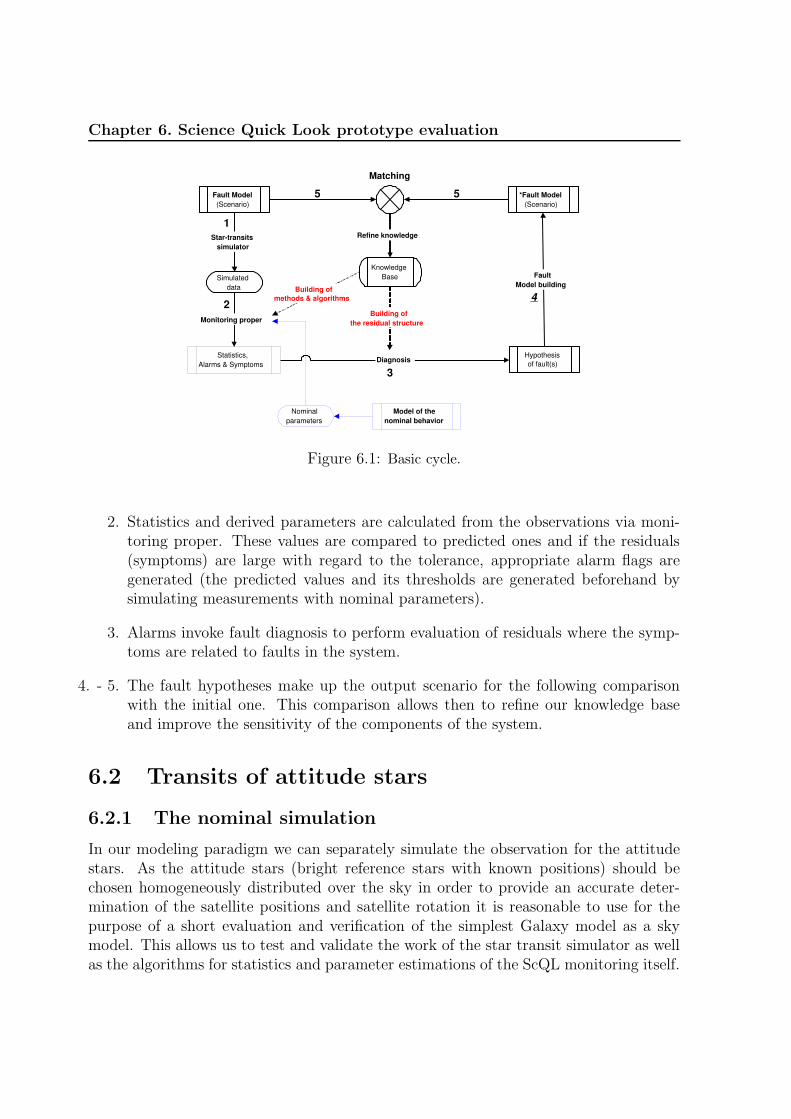
DR

AFT

Chapter 6. Science Quick Look prototype evaluation

Fault Model (Scenario)

Simulated data

Star-transits simulator

Monitoring proper

Diagnosis Hypothesis of fault(s)

Fault Model building

*Fault Model (Scenario)

Matching

Refine knowledge

Knowledge Base

Building of the residual structure

1

2

3

4

5 5

Building of methods & algorithms


Nominal parameters

Model of the nominal behavior

Figure 6.1: Basic cycle.

2. Statistics and derived parameters are calculated from the observations via moni-toring proper. These values are compared to predicted ones and if the residuals(symptoms) are large with regard to the tolerance, appropriate alarm flags aregenerated (the predicted values and its thresholds are generated beforehand bysimulating measurements with nominal parameters).

3. Alarms invoke fault diagnosis to perform evaluation of residuals where the symp-toms are related to faults in the system.

4. - 5. The fault hypotheses make up the output scenario for the following comparisonwith the initial one. This comparison allows then to refine our knowledge baseand improve the sensitivity of the components of the system.

6.2 Transits of attitude stars

6.2.1 The nominal simulation

In our modeling paradigm we can separately simulate the observation for the attitudestars. As the attitude stars (bright reference stars with known positions) should bechosen homogeneously distributed over the sky in order to provide an accurate deter-mination of the satellite positions and satellite rotation it is reasonable to use for thepurpose of a short evaluation and verification of the simplest Galaxy model as a skymodel. This allows us to test and validate the work of the star transit simulator as wellas the algorithms for statistics and parameter estimations of the ScQL monitoring itself.

DR

AFT

Chapter 6. Science Quick Look prototype evaluation 105

Indeed, the simulated science data from the star transit simulator in the case ofthe simplest Galaxy model can be analyzed with respect to the analytically calculatedproperties of the model. If the calculated characteristics from the nominal simulateddata for the attitude star transits, by using the ScQL monitoring proper, reconciles withthe analytical ones, then the developed simulator is working correctly. If the analyticalsolution does not reconcile the simulated science data, the star transit simulator is notverified and we know that something is wrong in our model.

Figure 6.2: Window rate and residuals (in relative units) vs. time on the SM CCD array(CCDs mosaic) for a binsize 5 minutes (solid line histogram). Blue dotted line denotes theanalytically mean value. The calculated mean window rate from the simulated observationscience data flow (mean o. = 822.89) coincides with the value derived from the analyticalmodel (mean m. = 822.86).

In figures 6.2 – 6.4 we present the number of downloaded windows of the attitudestars Nw and its residuals rw. The data stream is generated with the nominal parametersof the model of the satellite. The histogram, presented in fig. 6.2, shows the window ratefor the whole mosaic for two complete rotations of the DIVA satellite (4 hours) calculatedwith the binsize δt of 5 minutes. The calculated mean value o. = 822.89 of downloadedwindows from this simulated data stream coincides with that value m. = 822.86 that isderived from the analytical calculation. It demonstrates that the numerical model of thestar transits works properly, delivering the corrected data flow of the science data (inour study these are data from SM1 and SM2 mosaics). This statistics is an aggregationof the statistics from 8 individual CCD chips (see fig. 6.3). If there are wrong number ofthe downloaded cut-out windows of the chip n inside a special interval over m ∈ [0, 255]an ADU chain failure will be responsible for this fault (each CCD chip consists of 2ADU chains). In the case of the nominal simulation, the statistics on the level of theADU chain will give the window rate such as on the figure. 6.4, where the downloadedwindows from the upper ADU chain of the chip 1 is presented.

In the diagnosis, the statistics for any ADU chain will be taken as an elementary

DR

AFT


Figure 6.3: Window rate and residuals (in relative units) vs. time on the SM CCD chip for abinsize 5 minutes (solid line histogram). Blue dotted line denotes the analytically mean value.The calculated mean window rate from the simulated observation science data flow (meano. = 103.70) coincides with the value derived from the analytical model (mean m.= 102.86).

Figure 6.4: Window rate and residuals (in relative units) vs. time on the SM CCD ADUchain for a binsize δt = 5 minutes (solid line histogram). The blue dotted line denotes theanalytically determined mean value. The calculated mean window rate from the simulatedobservation science data flow (mean o. = 52.23) coincides well with the value derived from theanalytical model (mean m.= 51.43).

DR

AFT


quantity for all other calculated aggregation states while each ADU chain of the CCDmosaic has its own power supply and can be thus considered as the smallest ”active”element of the CCD mosaic. Nevertheless we compute analogous quantities over subsetsof the CCD mosaic measurements with the pixel size array smaller than one ADU chain(see in previous chapter section 5.2.2 item 4). Together with analyse of the full mosaicimage, that in the case of DIVA must be transmitted each 30 min, this statistics helpsto point out where the reason for a deviation from expected values be located on theCCD, i.e. to find out bad pixel regions.

6.2.2 Monitoring of TDI clock stroke rate adjustment

As described in the previous chapters, a maladjusted shifting of charges in the CCDs,transporting the charge at a different speed across the CCD smears out the star images.If the shifting of the charge on the CCDs does not match the actual rotation of thesatellite but this mismatch is not yet large enough to initiate the jet-firing then theTDI clock stroke rate should be tuned so that it is synchronized with scan-speed of thesatellite. In the star transit simulator we included the emulation of the work of the

Figure 6.5: The calculated (known) scan speed of the satellite with its uncertainties. In thisaxample an abrupt increase of the true scan speed is simulated on 30 May 2005 at 01:00:00UTC. The picture shows the determination of this effect by the ScQL software. Error barsrefer to mean errors (binsize 2 min.).

on-board software that monitors and adjusts (if necessary) the TDI clock stroke rate,using the transits of attitude stars (see section 4.8.7 of Chapter 4). In its turn the ScQLmonitoring on the ground verifies the correctness of these actions, using science and

DR

AFT


house keeping data. On the figure 6.5 the calculated speed of the satellite in the scan

Figure 6.6: Calculated (known) TDI clock stroke rate (left panel) and its residuals (rightpanel) vs time (binsize 2 min). Left panel: known TDI clock stroke rate with its uncertainties(bars). Yellow area denotes a small time interval (4 min) when the blurred images are delivered.Right panel: solid line histogram is the residuals of TDI clock stroke rate, that confirms thecorrectness of the work of the on-board software; dot-dashed histogram is the residuals of theTDI clock stroke rate in the case of a permanent maladjusted shifting of CCD charge.

direction is shown. To check the rotation of the satellite we take a time interval δt of2 minutes in our simulator. This is enough from the statistical point of view becausethe number of star transits for one million, homogeneously distributed over the sky(attitude stars) is about 330 (from both FOVs) . The ScQL monitoring uses the sametime interval to prove the calculations of on-board software1.

In our simulation scenario we introduced an abrupt increase of the scan speed after60 minutes. As one can see from the histograms on figure 6.6 the on-board softwarereacted correctly to this event. Firstly, it determines that the true TDI clock strokerate is not synchronized with the scan speed. On the left panel the calculated (known)TDI clock stroke rate exceeds the threshold (dotted red line). At the next 2 minutestime interval it proves whether the new scan speed is stabilized2. If yes (our case), theknew adjusted TDI clock stroke rate is set up as a true one. Thus, due to the changesof the scan-rate the instrument delivers the blurred images during 4 minutes (yellowarea) and then it is returned to the nominal status with a new true TDI clock stroke.

1In the ScQL monitoring the different time interval can be used to calculate the speed of the satelliteif necessary.

2It might be reasonable to check whether the speed is stabilized or not during several time intervals

DR

AFT


The residuals (solid line on the right panel) of TDI clock stroke rate, calculated in theframework of the ScQL monitoring system, confirms the correctness of the work of theon-board software. Otherwise, if the on-board software doesn’t adjust the TDI clockstroke the residuals would be permanent demonstrating of exceedance of the threshold(dot-dashed line) and therefore alarm would be arised by the ScQL monitoring system.

6.3 All star transits

6.3.1 The nominal simulation in the framework of the multi-

component Galaxy model. Time-varying thresholds.

The next stage for the evaluation of our monitoring system is to feed it by generating thescience data of the observations using a multi-component Galaxy model (the simulatedsky3). In the framework of this model our star transit generator can provide star counts

Figure 6.7: An illustration of the simulation of the band sky for one run (sample). Thispicture shows four sky subareas (the total number of which is 252) and the band of starsfor one sample of the sky map. The sky map is simulated according to the multi-componentGalaxy model in a given sky band defined by the nominal scanning law. A total number of 50runs are carried out in order to calculate the expected mean values of the star transit alongthe band of stars. An average total number of stars in one band is about 1.7 · 105 whichcorresponds to about 7 · 105 star transits in one complete rotation of the satellite. To simulate2 hours of observations takes 16 minutes of CPU time on Dell Inspiron 5150, powered by themobile Intel Pentium 4 processor at 3.06GHz with hyper-threading technology.

3The simulated sky is used in the star transit simulator instead of the known sky.

DR

AFT


down to the faint limiting magnitude of the instrument. According to the procedureof the multi-component sky map simulation, described in Chapter 4 section 4.3, thenumber of star transits is derived using different stellar density which was computed perarea unit at the sky for different magnitude intervals. In our practical implementationwe present the sky divided into Nsubareas = 252 subareas. In order to calculate andto evaluate residuals in this case one needs first of all to calculate the expected meanvalues of the rate of the star transit along the given sky band (the sky band is determinedaccording to nominal scanning law).

To do this we have to run the star transit simulator for a number of samples. Thesamples are produced by populating scanned subareas (see fig. 6.7) (which are observedby the satellite at a given period of time) according to the appropriate functions mod-elling the spatial and brightness distributions of the stars on the sky.

As an example we show the window rate of the full SM CCD mosaic calculated fromthe simulated science data. We take the same stretch of time as we used to demonstratethe crossing of the attitude stars in previous section. But we restrict ourselves to displaya total elapsed time of two hours to keep things legible. Figure 6.8 shows how manywindows arrive at each two-minute interval. The typical peaks can be explained bythe fact that the distribution of the stars is not homogeneous, the density is highestwhen scanning in the equatorial plane of the Galaxy. We have four peaks during afull rotation of the satellite in two hours because the main instrument simultaneouslyobserves two fields-of-view4 separated by 97.1 degrees. Each dot on the upper panel offigure 6.8 stands for one star transit run (the solid line represents the mean value). Atotal number of 50 runs with different samples of the star band were carried out in thiscase. In the lower panel of the same figure the expected mean value of the simulatedwindow rate and its standard deviation are shown. These standard deviations set upthe time-thresholds for the following evaluation of the residuals in the case of our multi-component Galaxy model. (Two hours of simulation takes 16 minutes of CPU time onDell Inspiron 5150, powered by the mobile Intel Pentium 4 processor at 3.06GHz withhyper-threading technology.)

After this, we simulate observations in the fault-free mode of the instrument (seefigure 6.9 upper panel). The lower panel of figure 6.9 represents the residuals; the meanwindow rate is shown as a reference (dotted line at rw=0). We displayed a 1-σ and a 3-σinterval (green- and red-dashed line respectively) around the mean value that representsthe time-varying alarm thresholds. The solid line is the residual computed by comparingthe simulated fault free simulated observation with the expected (predicted mean) value.

4The overview of the instrument can be found in Chapter 1 section 1.4.

DR

AFT


Figure 6.8: Window rate vs. time on the SM CCD array (binsize 2 min). Upper panel: (1) theblack dots – nominal window rates based on 50 different samples of the band sky simulationaccording to the multi-components Galaxy model (see sec. 4.3 of Chapter 4) and (2) the bluesolid-line histogram – the calculated predictive (mean) nominal window rate. Lower panel:the predictive window rate and its standard deviation (error-bar).

DR

AFT


Figure 6.9: Nominal. Window rate vs. time on SM CCD array (binsize 2 min). Upperpanel: (1) the blue solid-line with error-bars – the predictive window rate and (2) the blacksolid-line histogram – the simulated nominal window rate. Lower panel: (1) the black solid-line histogram – the residuals rCCDsw (see f. (5.1) in sec. 5.2.2 of Chapter 5), (2) the greendashed-line histogram and (3) red dashed-line histogram are the time-varying thresholds onthe level of 1σ and 3σ correspondingly. All fluctuations of the nominal window rate residualsare in the framework of 3σ.

DR

AFT


6.3.2 Monitoring of the window rate: an abrupt, an incipientand an intermittent fault.

We now introduce some simple faults into the simulated science data (an abrupt, anincipient, and an intermittent fault) and watch the reaction of the monitoring systemcalibrated with the measurements of the nominal star transits.

After approximately 60 minutes of operation, we simulate an abrupt fault (see fig-ure 6.10) decreasing the window rate (introducing the malfunctioning of a part of theCCD array). Figure 6.11 (for intermittent faults between 20 to 50 and 90 to 110 minutes)and figure 6.12 (for an incipient fault after 50 minutes) show a similar picture.

The monitoring system reacted to these events, when the residual signals went overthe threshold of 3σ. As a consequence, alarms were raised. For the abrupt failure thefour CCD chips (SM1: n=1 and n=2; SM2: n= 5 and n=6) were introduced to bedamaged and the alarm status is defined after 60 minutes. For the intermittent faults(fig. 6.11) the system goes into alarm status for the duration of the faults and revertsback to normal after they are over. In this case the number of the damaged CCD chipsis four (SM1: n=1 and n=2; SM2: n= 5 and n=6) for the time interval between 20 to50 minutes and three (SM1: n=1 and n=2; SM2: n= 5) for the time interval between 90to 110 minutes. We should stress here that the number of the simultaneously damagedareas of the CCD array which were introduced in the considered failure scenarios, iscovered a large area so that the faults could be detectable using only the statistics forthe whole CCD mosaic. It was done for the demonstration purpose because (as it hasbeen mentioned earlier) the statistics for the full CCD array is an aggregation of theCCD chips (or ADU chains) and, therefore, is not sensible to detect a fault for thesingle chip (or ADU chain). Indeed, based only on the statistical thresholds for the fullCCD array in the case of the incipient fault (fig. 6.12) the alarm would arise only after60 minutes whereas a damage of the first chip was introduced after 50 minutes in oursimulator. Moreover, it then go back to normal status for a short time, to reach analarm status only after 70 minutes (as shown in fig. 6.12).

The hierarchical structure of the SM CCD array for the ScQL monitoring

To react to this event promptly the ScQL monitoring calculates the residuals on thelevel of the individual CCD chips. In the figure 6.13 the residuals of the window ratefor chips are plotted for the given case of the incipient fault. It can be seen that thisfault is a composition of abrupt failures of four chips of the SM2 CCD. As the residualsignal of the window rate from SM2 CCD chip 5 exceeded its threshold, the ScQLmonitoring system switched to an alarm mode at the time 00:50:00 (the time of thefirst damage of the CCD mosaic was introduced in the fault scenario) and the systemremained permanently in this alarm status. In the case of the failure on the level ofADU chain appropriate residuals will be generated and evaluated in the same way.

Certainly, this hierarchical logic for the fault detection is somewhat redundant be-

DR

AFT


Figure 6.10: Abrupt fault. Window rate vs. time on SM CCD array (binsize 2 min).Upper panel: (1) the blue solid-line with error-bars – the predictive rate window, (2) the blacksolid histogram – the incorrect window rate. Lower panel: (1) the black solid histogram –the residuals rCCDsw (see f. (5.1) in sec. 5.2.2 of Chapter), (2) the green dashed-line histogramand (3) red dashed-line histogram are time-varying thresholds on the level of 1σ and 3σcorrespondingly. The abrupt decrease of the the whole CCD mosaic window rate is simulatedas a damage (or shut down) of the four CCD chips (SM1: n=1 and n=2; SM2: n=5 and n=6)on 30 May 2005 starting at 00:10:00 UTC; the considered fault-scenario covers time intervalof 2 hours [00:00:00, 02:00:00] UTC.

DR

AFT


Figure 6.11: Intermittent fault. Window rate vs. time on SM CCD array (binsize 2min). Upper panel: (1) the blue solid-line with error-bars – the predictive rate window,(2) the black solid histogram – the incorrect window rate. Lower panel: (1) the black solidhistogram – the residuals rCCDsw (see f. (5.1) in sec. 5.2.2 of Chapter), (2) green dashed-linehistogram and (3) red dashed-line histogram are time-varying thresholds on the level of 1σand 3σ correspondingly. The intermittent fault of the window rate on whole CCD mosaic issimulated as a the temporarily shutdown of the four (SM1: n=1 and n=2; SM2: n= 5 andn=6) and three (SM1: n=1 and n=2; SM2: n= 5) CCD chips on 30 May 2005 at [00:20:00- 00:50:00] and [01:30:00, 01:50:00] UTC correspondingly; the considered fault-scenario coversthe time interval of 2 hours [00:00:00, 02:00:00] UTC.

DR

AFT


Figure 6.12: Incipient fault. Window rate vs. time on SM CCD mosaic (binsize 2 min).Upper panel: (1) the blue solid-line with error-bars – the predictive rate window, (2) the blacksolid histogram – the incorrect window rate with the degradation of the SM CCD mosaic.Lower panel: (1) the black solid histogram – the residuals rCCDsw (see f. (5.1) in sec. 5.2.2 ofChapter), (2) green dashed-line histogram and (3) red dashed-line histogram are time-varyingthresholds on the level of 1σ and 3σ correspondingly. The decrease of the the whole CCDmosaic window rate is simulated as a consequent damage (or shut down) of the CCD chips onSM2 on 30 May 2005 starting at 00:50:00, 01:00:00, 01:20:00, 01:40:00 UTC; the consideredfault-scenario covers the time interval of 2 hours [00:00:00, 02:00:00] UTC.

DR

AFT


Figure 6.13: The residuals of the window rate on the chip level for the case of the consequentdamage (or shut down) of the chips on the SM2 mosaic (see also figure 6.12).

DR

AFT


SM CCD array

SM1 CCD SM2 CCD

CCD chip1 CCD chip2 CCD chip3 CCD chip4 CCD chip5 CCD chip6 CCD chip7 CCD chip8

ADU-l ADU-u ADU-l ADU-u ADU-l ADU-u ADU-l ADU-u ADU-l ADU-u ADU-l ADU-u ADU-l ADU-u ADU-l ADU-u

Figure 6.14: Hierarchical structure of the SM CCD array for monitoring of the science data.

cause the complete information for the residual evaluation can be obtained from thestatistics generated on the level of ADU chain5. However, such hierarchical represen-tation (see fig. 6.14) allows to obtain a more synthesized display of the data and tofacilitate the operator-astronomer the understanding of the state of the instrument.

Monitoring of the science data from an individual FOV

To make our hierarchical approach complete we will also calculate separately the resid-uals for two field-of-views (preceding FOV and following FOV) so that each FOV canbe supervised individually.

The given concept of the DIVA main instrument was designed in such a way that thestar light from both FOVs, combined on the one focal plane, could not be automaticallyidentified to which FOV it belongs. To do this the data treatment should be carried outin the framework of pipeline data reduction at the Data Center. But, one can calculateit easily for the attitude stars in the framework of the ScQL because their positions areknown a priori. However, in the case of Gaia, the viewing directions of both telescopesoverlap on a common focal plane with a shift of about 50 mm across-scan so that thestar images from each field-of-view can be uniquely identified without any additional

5It should be worth to note that the statistics for the small pixel blocks provides us with usefulinformation as for example CCD pixels degradation, but it will rather be used for a supplementarylong-term analysis and should not be considered as the monitoring parameters that are crucial for theperformance of the mission.

DR

AFT


Figure 6.15: Overview of the Gaia Astro focal plane. The two Astro telescopes share thesame focal plane: Astro field-1 is the area indicated in red, Astro field-2 is outlined in green.Three functions are assigned to the focal plane system: (i) the Astrometric Sky Mapper,which detects object entering the field of view, and communicates details of the star transitto the subsequent astrometric and broad-band photometric fields; (ii) Astrometric Field (AF),devoted to the astrometric measurements; (iii) the Broad Band Photometer (BBP) whichprovides multi-color broad-band photometric measurements for each object. The resultingfocal plane design consists of a mosaic of 180 CCDs with pixel of 10µm along scan × 30µmacross scan size (44.2 mas × 132.6 mas). From left to right: the first columns are for the skymappers with the following orange area of the CCDs for astrometry (analogue of DIVA SMCCDs); the last five columns are for broad-band photometry.

DR

AFT


object recognition procedure.

Like in the case of DIVA, stars crossing field are detected by the sky mapper (calledin terms of Gaia astrometric sky mapper), and then observed in the predicted windowingmode across the main CCD arrays (astrometric field), which is related to DIVA SM2.The sketch of Gaia’s focal plane is plotted on the figure 6.15 (see details in [43], [4]).Figure 6.16 illustrates the failure of preceding FOV that causes the homogeneous windowrate decreasing in the time interval of 20 minutes (see upper panel). According to ourhierarchical monitoring logic, the generated residuals for the preceding FOV (left panel)allows to detect and to identify this fault’s occurrence.

6.3.3 Monitoring of the star brightness

Assuming now that we obtain a wrong (small) number of windows from CCD array thatneither can be explained by complete chip (or ADU chain) damage nor by the problemwith the field-of-views. We introduced the high background during 20 minutes in ourstar transit simulator for the whole CCD array. So, the derived decreasing of the windowrate (or increasing of its residuals, figure 6.17) is also homogeneous in all chips of theCCD mosaic as it was in the case of the failure of the preceding FOV. The brightness ofthe stars can provide us with additional information to identify this failure. To monitorthe brightness of the stars we calculate the cumulative brightness distribution function ofobserved stars and compare it with the expected one by means of Kolmogorov-Smirnov(K-S) statistic. The constructed cumulative distribution functions are plotted on thefigure 6.18 (upper panel) for an interval of one complete rotation of the satellite. TheK-S statistic D, and the significance level ”prob” (see the formula (5.2) from Chapter 5)for the null hypothesis, that the data sets are drawn from the same distribution, are alsopresented on at: a small value of the prob shows that the cumulative function of thebrightness distribution of the observed data (black line) is significantly different fromthat of the expected (nominal). On the lower panel of the same figure the absolute valueof the difference between two cumulative distribution function helps to point out theinterval of the magnitude where it rises above the calculated greatest distance D of thetwo different nominal data samples (red dotted line). In principle, the most probablescenario that causes a wrong brightness distribution is a high background and/or a badsignal-to-noise ratio of CCDs. It gives the lack of faint stars and affects the tail of thedistribution. So, to identify finally the considered failure we calculate the number of thestars of a different brightness interval at the time when the decreasing of the windowrate took place. The derived value of the faintest magnitude Vlim (see histogram onfigure 6.19) of the observed stars at the this time period is too small and correlates withthe fact of too small window rate.

Thus, after disproving of the null hypothesis for a standard pre-defined time intervalby means of the K-S statistic, that demonstrates a good sensitivity in finding shifts ofbrightness distribution, the problematic time interval is checked.

DR

AFT


Figure 6.16: The decrease of the window rate on the whole CCD array (upper panel) is due tothe temporal problem with the preceding FOV (PFOV) of the main instrument. The residualsof the window rate from the preceding FOV (left panel) together with the residuals of thewindow rate from the following FOV (FFOV) (that shows no anomaly (right panel)), identifythis failure’s occurrence. Note: in the case of DIVA this failure can be only identified forattitide stars.

DR

AFT


Figure 6.17: The residuals of the window rate of the CCD array. The decrease of the windowrate on the whole CCD mosaic is due to the simulation of the high background in time interval[01:00:00, 01:20:00] UTC.

6.3.4 Monitoring of the star centroids

SM CCD rows

Let us examine now some image parameters from downloaded windows. But before, wewould like to mention that additionally to the hierarchical representation of the CCDarray for the monitoring of the science data we organized CCDs in rows (in pairs) inthe context of the ScQL. The reason for this is that stars detected on the SM1 mosaicare predicted on SM2 mosaic, so windows are cut out from one CCD of SM1 are relatedto windows from other CCD mosaic in the same CCD row. In this sense CCD rows canbe considered as a unit for important ScQL monitoring tasks. These related windows inthe case of the SM CCDs mosaic create the following chip pairs (see also fig. 4.15 fromthe Chapter 4): (SM1 chip 1 – SM2 chip 5), (SM1 chip 2 – SM2 chip 6), (SM1 chip 3 –SM2 chip 7), (SM1 chip 4 - SM2 chip 8).

To make the most of the image data of a window it should contain as much signalof the observed star as possible. Thus, the star centroid should be located in the centerof the cutted window. On the figure 6.20 the mean centroid of downloaded windowsfrom the nominal two hours simulation are presented. The centroids match the windowcenter with some positional error budget6. A bit shift that changes some data in theinstrument calibration can provoke that the predicted pixel coordinates of the windowto be extracted from SM2 CCD mosaic are changed and therefore the window cutting

6The error budget is taken about 1 pix.

DR

AFT


Figure 6.18: Unbiased estimators SN (V ) of the cumulative function for the two brightnessdistribution are constructed. The statistic D is defined as the maximum value of the absolutedifference between two distributions (see text).

DR

AFT


Figure 6.19: The histogram of the brightness distribution for the same time interval as infigure 6.17. The observed star histogram demonstrates an absence of faint stars starting fromVlim = 9 mag.

algorithm cuts out the wrong pixel stream area. In the extreme case, the shifts in thepredicted kw completely displace the windows to be cut out so that the start image isno longer situated in it, i.e. the empty windows will be extracted.

Identification of dual failure from monitoring of star centroids

As a last failure scenario we will consider a case of dual failure in which two failures,affected the position of the star centroids, occur simultaneously.

Firstly, we suppose that the detection algorithm (or cut-out algorithm)7 works im-properly and gives a false kw of the windows on the whole SM1 mosaic. If this slightshift is equal 2 pixels, then the predicted window pixel edge kw on the all chips of theSM2 mosaic will be systematically shifted and therefore the along-scan mean centroidCK of SM2 mosaic should be at about 8 pixel (see figures 6.21 and 6.22). Based on thisstatistics the ScQL monitoring system generates appropriate residuals and switches toan alarm mode with a diagnostic solution that either the detection or cut-out algorithmfor the detection mode on SM1 mosaic works improperly8. Furthermore, the systemwill detect the difference between expected values of the mean centroid position of theimages for the pair of chips (1 – 5). The expected position of the along-scan mean

7For the moment, we are not able to identify which one of these two algorithm works improperly.8This scenario is a

DR

AFT


Figure 6.20: Along-scan Ck and across-scan Cm centroids vs. time on SM CCD mosaic fora nominal simulation (dots on the left panels); the histograms (green lines) are the averagecentroid position CK and CL (binsize 2 min). On the right panel are the appropriate residuals(black line histogram) and its thresholds (red dashed line).

DR

AFT


Figure 6.21: The average centroid positions CK (green line histogram) and its residuals (blackline histogram) for the following rows (pairs) of CCD chips: [(1–5), (2–6)] in the case of thedual failure scenario. Dots are along-scan centroids Ck. Yellow line histograms (chip 5) areexpected centroid positions CK (and its residuals) if only the failure of the detection algorithmtook place.

DR

AFT


Figure 6.22: The same as on the figure 6.21 but for the other rows of CCD chips: [(3–7),(4–8)].

DR

AFT


centroid of the chip 5 in the case of detected failure of the detection algorithm is shownby yellow line histogram on the figure 6.21. This indicates that that the calibration dataof the along-scan offsets between the consecutive CCDs is changed of about 1 pixel (seethe geometric arrangement of SM CCDs on figure 4.15 from the Chapter 4.

Thus, the result of the failure identification from the diagnosis system will be twofolded:

• The detection algorithm failed. The on-board detection (or cut-out) algorithm hasbeen working improperly in the ’detection mode’ on the SM1 mosaic since 30-05-2005 00:01:30. Possible intervention is to reload the software. Alert the FirstLook.

• The calibration data is damaged or changed. The along-scan offsets between thechips (1 – 5) has been changed or the calibration data has been corrupted. Pos-sible intervention: upload the calibration data; if the problem persists, the newcalibration data should be produced in the framework of the First Look. Alert theFirst Look.

Note that the incorrect attitude will also produce badly predicted windows, smearingout the star image while the shifting of charges in the CCDs will no longer match thereal scan speed. But the centroid positions would not have a systematic shift in thiscase.

6.4 Summary

In this chapter, we have presented the evaluation of the developed prototype of theScQL monitoring system. The system was extensively tested, feeding simulated sciencedata generated by the star transit simulator into it. The nominal simulations have beencarried out to derive computational solutions of what should be considered as fault-free parameters. The calculated standard deviations set up our modeled time-varyingthresholds and confidence level for the ScQL evaluation phase. These time-varyingthresholds (for the case of the rate of the downloaded windows/images) follow Poisson’sstatistics because our knowledge about the sky (in the simulator) is restricted by averagestellar coordinate and stellar magnitude distributions. This knowledge, however, will besubstantially improved after half a year of observations when the first sphere solution isperformed. This will allow us to refine our model and determine thresholds that are asclose as possible to the nominal case (fig. 6.23).

According to the proposed evaluation basic cycle, we have simulated different failuresituations in the framework of the star transit simulator to verify the reaction of thesystem. The simple hierarchical data representation seems to be effective and reliablefor the purpose of fault identification and provide a synthesized display of the data thatfacilitate the understanding of the instrument status.

DR

AFT


Observations


Fault Model building

Monitoring proper

Hypothesis of fault(s) Diagnosis

*Fault Model (Scenario)

Star-transits simulator

Simulated data

Monitoring proper

1

2

3

4

Matching Refine knowledge Knowledge

Base

Building of the residual structure

5

6

6

Building of methods & algorithms

Improving of the Model of the satellite

Building of methods and

algorithms


Figure 6.23: Learning diagnostic knowledge cycle.

DR

AFT


DR

AFT

Chapter 7

Conclusion and Outlook

This thesis considered different aspects of the development of the monitoring systemfor rapid assessment of the performance of scanning astrometric satellites. A scan-ning spacecraft needs a global, coherent, interleaved reduction and calibration of manymonths of measurements to reach their target levels of precision. It is therefore, on onehand, very difficult to immediately assess the proper functioning of all elements at therequired levels of precision and stability. It is, on the other hand, for the same reasonof utmost importance to quickly get a handle on the inherent quality of the elementaryscience measurements. So, monitoring of various kinds is required to continuously checkthe correct operation of a scanning satellite, both as individual components and as acomplete system. To perform the preliminary assessment of the main instrument of thesatellite in quasi real time constraints the concept of the Science Quick Look monitoringhas been developed in the framework of this thesis. The aim of our study was mostlyto explore basic monitoring properties and identify specific features for such a class ofspace missions but not to produce an operational ScQL monitoring system for a givenscanning science astrometry satellite. We have shown that our model of fault detection(monitoring proper) is effective in the prototype of the system supervision of the sci-ence data of the DIVA astrometry satellite. It can be easily used in conjunction withfault-identification (diagnosis) for automatically identifying the nature of a failure afterdetecting it occurrence. The developed concept is quite general and is applicable toother related scanning space mission such as Gaia.

This chapter summarizes the work presented in this thesis. The main results andconclusions are reviewed, directions for further investigations are presented.

7.1 Conclusion

The following number of items can be drawn based on the accomplishments of thisthesis.

O In order to guarantee a high level of precision when collecting scientific data during

131

DR

AFT

Chapter 7. Conclusion and Outlook

a space-based astrometry mission, the quality of the data needs to be checkedconstantly. The first goal of our work was to study the problem of monitoringscientific data considering the specific characteristic of a astrometry space mission.As a result of this study we employ a model-based approach, where we do not relyon empirical knowledge about symptoms and faults but on fundamental knowledgeof the considered domain. We have explored the modern state of this approachand one thing became clear from the literature that there is no universal methodto cope with all possible situations. We favor a model-based approach, in whichwe can extract diagnostic clues from discrepancies between predicted behavior andobservations. This approach is rather natural for a scientist as this is how he orshe usually solves scientific problems. There are also shortcomings of the puresymptom-based approaches, the main one being that it is difficult to comprehendwhy a system arrives at a certain conclusion.

O The design of the model-based ScQL monitoring was driven by careful analysisof the spacecraft domain, paying attention to the specific characteristics of anastrometry space mission. The distinguishing feature of the ScQL monitoring is toperform an indirect control of the work of the components of the main instrumentsatellite by collecting, analyzing and interpreting the astrometry observations.Thus, at the core of the ScQL model is star transit simulator that mimics thebehavior of satellite and simulates its observations. It also guides the developmentof the two other parts of our system: monitoring proper and diagnosis.

– The star transit simulation is responsible for describing the predicted behaviorof the satellite. It is also used for generating simulated data during thedevelopment of the system (as no observed data is available yet).

– Monitoring produces statistics and derived parameters from observations.These values are compared to predicted ones and if the differences are toolarge, the system raises alarms.

– In the diagnosis step the symptoms (in the form of residual structures) gener-ated by monitoring are related to faults in the system by residual evaluation.

O The complete model of the observations is an extremely challenging task. The firststep towards this direction is the model implemented in our star transit simulator.It consists of the model of the Galaxy, the structure and behavior of the maininstrument of the satellite and the model of the scanning strategy of the satellite.Our modeling approach achieves a broad coverage of monitoring of the on-boardinstrument hardware and software by coupling the purely quantative model withthe semi-quantative approach. Indeed, keeping the description of the work of somecomponents of the instrument at the high level of abstraction permitted to createan extended skeleton of the ScQL monitoring at this stage of the project (whenthere is a lack of the detailed information of the behavior of some components).

DR

AFT

Chapter 7. Conclusion and Outlook 133

O Maintaining the knowledge for such a complex system was also a challenging task,as small changes in the design may necessitate revisions in a large part of theknowledge base. In our model we introduced strong definitions and parameteriza-tions of the entities related to the model of the observed environment (sky) andinstrument. Following this formalism one can modify the ingredients of the modelof the system to generate the more detailed star transit simulation and thereforeexpand the capability and accuracy of the ScQL monitoring itself.

O In the early stages of the DIVA project, we were faced with the need to establishthe strategy for the DIVA data reduction software (pipeline) based on a relationaldatabase. In order to combine the strength of various programming languages,minimize the efforts and to reuse the components we proposed to use the con-ception of mixed-language programming. In the ScQL monitoring we successfullyapplied the MLP approach that allowed us to build a flexible and compatible withthe database software.

O Upon analyzing the list of the main quantities of the statistics and parameterswhich are analyzed at ScQL monitoring, we determined the architecture of themonitoring proper mostly based on the IDL (Interactive Data Language). Weadopted and modified the two main parts of Foundation Class Layer (FCL), Vi-sualizer and the Dataform, providing the user interface part and visualizing theoutput of the star transit simulation and statistics-generating components of ScQL.

O Our work focused on the monitoring part of the system, i.e., the diagnosis systemis not worked out as elaborately as its monitoring counterpart at the moment.Basically it consists of a set of 50 rules implemented in COOL (CLIPS Object-Oriented Language (tool) for building expert systems). Applying this tool for thedevelopment of our diagnosis part of the system will allow us to perform easilystructural testing of implemented rules that are found to be correct in syntax,unique in name and action, complete and consistent. But we do not consider atall the important aspect of the severity of the faults, this certainly should be thetask of further studies.

O The proposed design was demonstrated in the framework of the DIVA ScQL pro-totype with the scenario evaluation procedure. The evaluation was to determineif we succeeded in achieving our objectives to have a tool that assists the operatorin quasi-real to deduce the changes of the state of the satellite from the sciencedate, producing appropriate statistics and diagnosis.

The monitoring system was tested extensively by feeding simulated star transitdata into it and by generating and evaluating statistics. The evaluating procedure,based on the ”scenario – simulation – monitoring – diagnosis – matching” cycle,allows to watch and validate the reaction of the ScQL monitoring in terms offailure scenarios.

DR

AFT

Chapter 7. Conclusion and Outlook

The nominal simulations have been carried out to derive computational solutionsof what should be considered as a fault-free parameters. The calculated standarddeviations set up our modeled time-varying thresholds and therefore the confidencelevel for the ScQL evaluation phase. These time-varying thresholds (for the caseof the rate of the downloaded windows) follow the Poisson’s statistics while ourknowledge about the sky is restricted by average stellar coordinate and stellarmagnitude distributions. This knowledge, however, will be substantially improvedafter half a year of observations when the first sphere solution is performed.

7.2 Outlook

The results of an evaluation of our system is very promising, so it will be worthwhile topursue further studies in this area. First of all the diagnosis part of our system must beimproved to bring it on par with the monitoring part. Second – as the DIVA projectwas stopped – we are able to adjust our approach to the next space-based astrometrymission, Gaia, which will be launched in 2012. Indeed, many aspects for the rapidassessment of payload and spacecraft health, developed in this work in the frameworkof DIVA project, are analogous to those in Gaia due to the fact that the main principleand basic geometry of the measurements are the same.

To build a complete ScQL diagnostic system with the sensitivity it will be extremelyvaluable to take into account the simulation at CCD pixel level (when the raw datawith images are generated) as well as some other technical issues like charge transferefficiency of the CCD, possible irregularities of the physical pixels, projection effectsfrom the sky to the focal plane, etc.

A successful completion of the ScQL prototype for the DIVA mission provides thebasis for our belief that a ScQL monitoring system for the larger project – Gaia – isachievable in terms of the developed concept. Building a ScQL monitoring system forGaia therefore would become a lot easier if the important steps have already been donein the DIVA project. It is evident, however, that this work has to evolve and grow,along with the concept of the Gaia satellite.

DR

AFT

Chapter 8

Appendix

8.1 The contribution of DIVA to astrophysics

The unique combination of homogeneous astrometric and photometric as obtained withDIVA is expected to have a huge scientific impact on many fields of astronomy, andnamely:

• calibration of stellar parameters (much better than available now)

• accurately measure numerous double stars

• discovery of nearby faint stars (e.g. brown dwarfs, metal poor subdwarfs, whitedwarfs)

• determination of the spatial distribution of stars in the local disk with that, mapthe spatial structure of extinction

• improve the calibration of RR Lyrae to help better determine the size of the MilkyWay to better determine the ages of the galactic globular clusters

• provide accurate proper motions (tangential velocities) of stars to better determinethe kinematics in the Milky

• obtain accurate stellar distances perpendicular to the Milky Way disk to get betterinformation on the vertical force Kz

• from the above two to investigate the mass contribution of Dark Matter

• improve the calibration of Cepheid stars to help better determine the distances ofother galaxies to better determine the value of the Hubble constant

• obtain an accurate proper motion for both of the Magellanic Clouds

135

DR

AFT

Chapter 8. Appendix

8.2 Window datation and Image Parameter Set

On the long way from raw DIVA telemetry to the final DIVA catalogue, the DIVA datareduction chain produces a lot of intermediate data of many different types [8]. The“atom” of data of a certain type is called a record. A record is a set of intimatelyconnected parameters, such as e.g. the individual pixels of a DIVA “window”, alongwith the time of observation and the number of the CCD chip.

The individual records must be organized into larger structures, which we call filesand which are described by parameters collected into file header records. Records, inturn, are composed of individual physical quantities, counters, flags etc., which we col-lectively call data items.

A specific data set (file or record) may by definition contain information from somepart of the mission only (e.g. a single “window” or the set of “windows” from a specificmission day), or else data derived from the whole mission (e.g. an object list or onerecord in an astrometric output catalogue). This depends on the type of data.

The science data for the ScQL expert system should get through initial treatment inorder to get image parameter sets. We describe here pre-processed data in more details.

8.2.1 Explanation of the data type descriptions

It gives descriptions (definitions) of the various data types. Every definition is dividedinto a verbal overview, including an estimate of the data volume, and some tables givingdetails. The tables describe the data in terms of records and files. This is a purely logical,not a physical description. It should not be mixed up with the technical storage andorganization of the data in the central data base. The data base crew is free to avoidduplication of data items, and to organize the data such that the necessary access modesrun quickly and smoothly.

In the data type description tables, each line defines one data item. The individualcolumns of the tables have the following meanings:

abbr.: shorthand designation of the data item (“abbreviation”).

name: full (but still short) name of the data item.

dimension: the array dimension if the data item is an array; a one-dimensionalarray is specified as e.g. -5:12, where the two numbers -5 and 12 denote the lower andupper limits of the element indices (the length of the array is 18 in this case); multi-dimensional arrays are specified as e.g. -5:12,1:10 (the array is two-dimensional, its totallength is 180 in this case). If nothing is written it means a single number.

type: the type of the data item (the array elements); possible values are I*2, I*4,R*4, R*8, Ch*n for integer, real and character (text string) data of different wordlengths; word lengths are given in bytes (2, 4 or n); data items of type logical or bitsare specified as I-type for the moment; with the actually needed number of bits givenin some instants.

DR

AFT

Chapter 8. Appendix 137

offset: offset of the data item from the start of a record in an exchange format file(in Bytes).

exch. format: machine-independent ASCII format (in Fortran notation) for thedata item, in files used for data exchange between different sites and/or computers

bounds: upper and lower limits for the possible values of the data item; strict boundsmust be distinguished from order-of-magnitude indications (the latter being indicatedby ∼ characters). A * means that there is no limit.

resol.: the numerical resolution needed; if applicablephys. unit: the physical unit in which the data item is represented; if applicabledescription: a more verbose description of the meaning of the data item; usually

not a complete definition in full detail.remark: pointer to remarks, either included at the bottom of the table (indicated

by the symbol *), or in some other document (indicated by the document number ortitle).

opt.: data items that are not necessarily present in a data record (“optional” items)are indicated by ‘yes’; the presence or absence of such items must be indicated bysome flag elsewhere in the record (or in the file header, if the presence or absence ischaracteristic of the whole file rather than the individual records).

8.2.2 Windows

The so-called windows are the central observational results produced by the DIVA in-strument(s). There is one window record per on-board-detected or -predicted star image,plus some special windows (see below). The windows have different sizes (see Table 8.3);they are created in varying rates. On average there will be about 200 records/second,but this varies between about 50 and 1500 records/second.

Mean number of windows:

96/s + 33/s + 14/s + 56/s + 27/s = 226/sSM SC SCzero UVl UVs total

The database will receive window data as well as all other sorts of GSOC outputs,in bunches. Thus the individual window records must be organized into larger windowfiles (tables), which are described by file header records, see Table 8.1.

The window records are described in Tables 8.2 and 8.3. The individual items con-tained in the window records fall into two or perhaps three categories, to be brieflyexplained in the following.

DRAFT

Chapte

r8.

App

endix

Table 8.1: Windows, Header Contents

abbr. name dimension type offset exch. for-mat

bounds resol. phys.unit

description remark opt.

production Ch*14 1s s start time at whichdata are written intothe DB

date in the form yyyymmd-dmmssin system time of theDB computer (ideallyUTC)

producer Ch*10 shorthand for the pro-cess creating the DBentryexamples may be:routine GSOC deliv-ery,manual replacement offaulty data,manual insertion ofmissing data

DRAFT

Chapte

r8.

App

endix

139

Table 8.2: Window, Record Contents, Part 1: Window Datation

abbr. name dim. type offset exch.format

bounds resol. phys. unit description remark opt.

kw I*4, 26 bit 1,...,∼ 64 000 000 running number of TDI clock stroke after thelatest reset, at the “lower left corner of thewindow

TD0201

kw I*2, 16 bit 1,...,* running number of the latest reset of k TD0201mw I*2, 9 bit number of CCD column, at the “lower left

corner of the windowTD0201

-12,...,523 for SM, SC-12,...,-1 and 512,...,523 for underscan region

-12,...,2059 for UV-12,...,-1 and 2048,...,2059 for underscan re-gion

n I*2, 5 bit 1,...,22 number of CCD chip TD02011,...,4 for SM15,...,8 for SM29,...,12 for SM313,...,16 for SC117,...,20 for SC221 for UVshort22 for UVlong

type Ch*1, 8 bit window type identifier TD0201for SMbit 0: normal windowbit 1: bright star windowbit 2: guest observer object (goo) windowbit 3: full-chip windowbit 4: attitude starbit 5: rate pair componentbit 6: predictedbit 7=0 for goo windows from fFoVbit 7=1 for goo windows from pFoVfor SCbit 0 - 6: decimal value =0 → full-chip win-dowdecimal value = 6 → zero-order windowdecimal value =7,...,84→ z-height of the win-dow, normal windowbit 7: attitude star windowfor UVbit 0: normal windowbit 1: full-chip window

DRAFT

Chapte

r8.

App

endix

Table 8.3: Window, Record Contents, Part 2: Pixel Values

abbr. name dimension type offset exch. format bounds resol. phys. unit description remark opt.

windowdatation

I*4, 3I*2,Ch*1

pixa pixel valuearray

2 dim., var. I*2, 16 bit 0,...,65 535 1 ADU ADU signal of one window, size de-pending on n and type

TD0201TD0251

for SM0:12, 1:7 normal window including

background (index 0)0:12, 1:17 bright star window including

background (index 0)1:28, 1:11 guest observer object window1:1024, -12:524 full chip window including

underscan regions (indizes−12,...,−1 and 513,...,524)for SC

1:1024, -12:524 full chip window includingunderscan regions (indizes−12,...,−1 and 513,...,524)

0:12, 1:7 zero-order window includingbackground (index 0)

0:12, 1:z-height normal window includingbackground (index 0), 7 ≤z-height ≤ 84 )for UV

-1:4, 1:4 normal window includingbackground (index −1 and0)

1:256, -12:2059 full chip window includingunderscan regions (indizes−12,...,−1 and 2048,...,2059)

pkey predictionkey

I*4, 3I*2,Ch*1

window datation of that SMwindow from which the posi-tion of this window was pre-dicted.only for predicted SM win-dows and all SC windows

DR

AFT


8.2.3 Image Parameter Set

Image parameter sets (IPS) are the main output of the pixel data processing task. IPSrecords are derived from window records. An IPS contains parameters of an actualimage of an astronomical source recorded in the pixel values of a window. Such pa-rameters are: centroid position (in pixel coordinates), brightness (amplitude, integratedphoto-electrons or ADC units), shape parameters (diameter, duplicity, diffuseness...),diagnostics (disturbed by cosmic ray, badly positioned in the window, truncated byCCD edge, ...). Details are defined by the pixel data processing task. The first versionat defining IPS records is given in Tables 8.4 and 8.5.

There can be several images in a window numbered by the index l, and thus severalIPS records derived from that window. There will be at least one IPS per window,although it can occasionally happen that there is no detectable image (in this case theIPS will contain dummy parameters).

The PICat number(s) give the preliminary identification(s) of the detected imagewith an object in the Preliminary Identification Catalogue (PICat). These numbers areproduced at the same time as the IPS itself.

Each IPS record must carry the window datation, the image numbering l, the windowidentification data (if applicable), and the PICat number(s) of the corresponding PICatobject(s), again if applicable.

The IPS fall into a large number of categories or types. Each of these types will beaccessed by different subsequent processing steps, and in very different ways. This mustcarefully be taken into account by the data base crew in setting up the organization ofthe IPS data organization.

8.2.4 Classification according to instrument type

• SM records for normal stars

• SM records for bright stars

• SC records

• SC zero-order records

• full-chip records

• guest observer object records

• UV-long records

• UV-short records

DR

AFT

Chapter 8. Appendix

8.2.5 Classification according to object type

• unknown object

• PICat object

• attitude star

• astrometric reference star

• photometric SM reference star

• photometric SC reference star

• photometric UV-long reference star

• photometric UV-short reference star

• guest observer object catalogue star

etc.; all categories of objects will have different usages in the data reduction chain(s).Analogously, images identified with a PICat object will be used differently from thenon-identified ones.

8.2.6 Special window types, non-object windows

In addition to the obvious classification of IPS according to instrument type (8.2.4) andobject type (8.2.5) there will probably be a few special types of windows which willproduce image parameters sets of a completely different nature. One example might beoccasional sets of complete CCD lines (the so-called full-chip windows). The pixel dataprocessing task would not derive observations of individual objects from them, but moregeneral things like the instantaneous background level (sky background brightness plusdark current) which may apply to more than one window of the ordinary types (8.2.4).They can also be used to check/optimize on-board image detection. Another possibleexample is CCD underscan windows from which the CCD bias and read-out noise levelscan be derived. Again this applies to a certain stretch of other window data.

The list of such data types has not yet been finalized, nor the frequency of theiroccurrence or the total amount of data in them. A first sketch of this subject can befound in [12].

8.2.7 Data quantity

SM-type windows:

Tables 8.4 to 8.5 give a realistic draft of the structure and contents of IPS data forSM-type windows.

DR

AFT


a) information repeated from raw data:

datation (k,m, n, type): 11B/windowmaybe identification (see 1.2.3): 2B/window (rarely present)

b) new information (see Table 8.5):

PICat identification (implying object classification): 4B/windowimage counter l: 2B/windowimage parameters proper and flags: 80B/window

SC-type windows (details still to be defined):

a) information repeated from raw data:

as for SM-type records

b) new information:

PIC identification: 4B/windowposition-dependent amplitude: 80× 2B/windowshape parameters: 6× 2B/windowflags: 2B/window

Data quantity

SM-type windows:

repeated: 11B/window = 0.11TB/missionnew: 82B/window = 0.81TB/mission

SC-type windows:

repeated: 11B/window = 0.02TB/missionnew: 174B/window = 0.29TB/mission

total new: 1.23TB/mission per versionIn other words, since 5 or 6 versions can be expected, the total amount of IPS data

may be as high as 6 to 8TB (possible mission prolongation not taken into account).

DRAFT

Chapte

r8.

App

endix

Table 8.4: Image Parameter Set, Header Contents

abbr. name dimension type offset exch. for-mat



versionnumber

I*2

production Ch*14 1s s start time at which dataare written into the DB

date in the form yyyymmd-dmmssin system time of the DBcomputer (ideally UTC)

producer Ch*10 shorthand for the processcreating the DB entryexamples may be:automatic pipeline pro-cessing,automatic reprocessing,manual repeat of a pro-cessing run

validation I*2 1,...,5

DRAFT

Chapte

r8.

App

endix

145

Table 8.5: Image Parameter Set, Record Contents

abbr. name dimensiontype offset exch. for-mat



windowdatation

I*4, 3I*2,Ch*1

l I*2, 2 bit 0,...,3 IPS running numberpicat PICat

identifierI*4 identification number of the

star in PICatcentroid position (pixel coordinates)

Ck 1:2 R*4 0,...,1 pixel centroid position in scan direc-tion reckoned from kw, suchthat κ = kw + Ck,computed with 2 differentmethods

Cm 1:2 R*4 0,...,1 eff. pixel centroid position in cross-scandirection reckoned from mw,such that µ = mw + Cm,computed with 2 differentmethods

brightnessI 1:2 R*4 0,...,* ADU amplitude, computed with 2

different methods1:2 R*4 ADU background

shape1:2,1:5

R*4 shape parameters, up to 5, de-pending on the method, e.g.duplicity, diameter, diffuse-ness, area

quality1:2 I*2, 8 bit diagnostics, up to 8 bit, de-

pending on the method, e.g.disturbed by cosmic ray, badlypositioned in the window,truncated by CCD edge

DR

AFT

Chapter 8. Appendix

8.3 Attitude and nominal scanning law

8.3.1 Attitude matrix

The attitude of the satellite is the orientation of the satellite system with respect to theICRS. It is expressed by the attitude matrix A, an orthonormal 3 × 3 matrix. Eachline of the matrix contains the equatorial (ICRS) direction cosines of one of the satellitesystem’s principal axes. Conversely, the columns of the matrix contain the directioncosines of the ICRS principal axes expressed in the satellite system. Symbolically:

A =

x’y’z’

ICRS

=(XYZ

)sat.syst.

(8.1)

where the prime denotes the transpose of a vector.Multiplying A with any vector u given in ICRS coordinates produces the represen-

tation of that vector in the satellite system:xyz

u

= A ·

XYZ

u

(8.2)

8.3.2 The nominal scanning law

The following parameters are needed to determine the attitude at the next apogeeaccording to the NSL:

a1 := −0.16378459 ,

a2 := −0.01307777 ,

a3 := 0.00123243 ,

a4 := 0.00012341 ,

b1 := 0.08215269 ,

b2 := 0.99006117 ,

b3 := 0.04045213 ,

e := 0.016714 ,

g1 := −0.04414 + 0.017201969d1 ,

K := 6.4 ,

L1 := 1.38691 + 0.0172021240d1 ,

R := 11.25 ,

ε := 0.409092804222328826 ,

DR

AFT


λ1 := L1 + 2e sin g1 +5

4e2 sin 2g1 ,

ν := ν + a1 cos ν + a2 cos 2ν + a3 cos 3ν + a4 cos 4ν

ν = ν0 +Kλ1 ,

ξ :=π

4,

Ω = Ω0 + 2πR (d1 − d0)− ν cos ξ + (b1ν + b2 cos ν + b3 sin 2ν)sin ξ

K,

where d1 is the apogee time in mean solar days from the reference epoch d0 adopted forthe NSL. Since λ1 may exceed 2π, λ1 modulo 2π should be used instead of λ1. ν0 andΩ0 are telecommandable constants fixing the NSL. The attitude according to the NSLis then

ANSL (d1) = D3 (Ω)[D2

(π2− ξ) [D1

(ν − π

2

)[D3 (λ1)D1 (ε)]

]]

with

D1 (φ) =

1 0 00 cosφ sin φ0 − sinφ cosφ

,

D2 (φ) =

cos φ 0 sin φ0 1 0

− sinφ 0 cosφ

,

D3 (φ) =

cos φ sin φ 0− sinφ cosφ 0

0 0 1

.

Multiplying this attitude matrix ANSL (d1) with any vector given in the equatorial coor-dinate system produces the representation of that vector in the body-fixed coordinatesystem of the satellite. For the back transformation the transposed matrix can be used,which is the inverse matrix of the attitude matrix.

DRAFT

Chapte

r8.

App

endix

8.4 DIVA main instrument

In the following tables the collection of parameters for DIVA main instrument as well as estimation of date rates arepresented:

Table 8.6: DIVA collection of parameters, Part 1 (general parameters)

1a) Common parameters, generalscan speed 180 ”/sec omegafields of view 2 N_fov

1b) Common parameters, derivedrotation period 120 min T_rot=360*3600"/omega/60sec

exposure time for one CCD transit 1.414 sec t_exp=M_w*scalpx/omega

2a) Optics, generalfocal length 11200 mm Faperture size in w direction 220 mm Daperture size in z direction 110 mm Hcenter of preceding aperture in z direction 95 mm z_prec

center of following aperture in z direction -95 mm z_foll

2b) Optics, derivedgap between apertures in z direction 80 mm gap=abs(z_prec-z_foll)-H

primary mirror, actual size in z direction 300 mm H_prim=abs(z_prec-z_foll)+H

primary mirror, max. dist. from opt. axis 186.01 mm R_prim=sqrt( (max(abs(z_prec),

abs(z_foll))+H/2)^2 + (D/2)^2 )

image scale in mm 18.42 ′′/mm scalmm=206265/f

image scale in pixels 0.249 ′′/pix scalpx=scalmm*pix_w/1000mum

image scale in eff. pixels 0.994 ′′/eff.pix. scaleffpx=scalmm*pix_eff/1000mum

DRAFT

Chapte

r8.

App

endix

149

Table 8.7: DIVA collection of parameters, Part 2 (general parameters)

3a) CCDs, generalpixel size in w direction 13.5 mu-m pix_w

pixel size in z direction 13.5 mu-m pix_z

on-chip binning factor in z direction 4 binningCCD chip size in w direction 1024 pixels M_w

CCD chip size in z direction 2048 pixels M_z

number of readout channels per chip 2 N_read

3b) CCDs, derivedCCD chip size in w direction 13.82 mm size_w=pix_w*M_w/1000mum

CCD chip size in w direction 4.24 arcmin size_w_arc=size_w/f*180/3,141593*60

CCD chip size in z direction 27.65 mm size_z=pix_z*M_z/1000mum

CCD chip size in z direction 8.49 arcmin size_z_arc=size_z/f*180/3,141593*60

effective pixel size in z direction 54 mu-m pix_eff=pix_z*binning

4a) Focal plane assembly, generaltotal number of chips in SM 8 chips N_SM

number of chips needing image detection 4 chips N_imadet

total number of chips in SC 8 chips N_SC

field of view width in z direction, SM 4 chips fov_sm

field of view width in z direction, SC 4 chips fov_sc

4b) Focal plane assembly, derivedtotal number of chips 16 chips N=N_SM+N_SC

field of view width in z direction, SM 33.95 arcmin size_fov_sm

field of view width in z direction, SC 33.95 arcmin size_fov_sc

DRAFT

Chapte

r8.

App

endix

Table 8.8: DIVA collection of parameters, Part 3 (data rates)

5) TDI, derivedTDI clock rate 724.0 lines/sec TDI_rate=omega/scalpx

TDI clock interval 1.381 msec TDI_time=1/TDI_rate*1000msec

5a) CCD data rates, generalnumber of data bits per pixel 16 bit bitpix5b) CCD data rates, derivedCCD data rate, SM 47.45 Mbit/sec dat_SM=N_SM*M_z/binning*TDI_rate*bitpix/106 Mpix

CCD data rate, image detection 23.72 Mbit/s dat_imadet=N_imadet*M_z/binning*TDI_rate*bitpix/106 Mpix

CCD data rate, SC 47.45 Mbit/sec dat_SC=N_SC*M_z/binning*TDI_rate*bitpix/106 Mpix

CCD data rate, total 94.89 Mbit/sec dat=dat_SM+dat_SC

6a) image rates, generalnumber of stars, SM, all sky 35 · 106 stars stars_SM

max/mean star density, SMSM (Milky Way) 3.3 dense_SM

min/mean star density, SMSM (galactic pole) 0.21 sparse_SM

number of stars, SC, all sky 12 · 106 stars stars_SC

max/mean star density, SCSC (Milky Way) 3.0 dense_SC

min/mean star density, SCSC (galactic pole) 0.23 sparse_SC

DRAFT

Chapte

r8.

App

endix

151


6b) image rates, derivedarea of sky per second, SM 0.113 sq deg skysec_SM=fov*N_SM*size_z_arc/60*omega/3600

area of sky per second,image detection 0.057 sq deg skysec_imadet=fov*N_imadet*size_w_arc/60*omega/3600

area of sky per second, SC 0.113 sq deg skysec_SC=fov*N_SC*size_w_arc/60*omega/3600

stars per second,SM, mean 96.0 stars/sec rate_stars_SM=skysec_SM*stars_SM/41253

stars per second,SM, max 316.8 stars/sec rate_dense_SM=skysec_SM*stars_SM*dense_SM/41253

stars per second,SM, min 20.2 stars/sec rate_sparse_SM=skysec_SM*stars_SM*sparse_SM/41253

stars per second,image detection, mean 48.0 stars/sec rate_stars_imadet=skysec_imadet*stars_SM/41253

stars per second,image detection, max 158.4 stars/sec rate_dense_imadet=skysec_imadet*stars_imadet*dense_SM/41253

stars per second,image detection, min 10.1 stars/sec rate_sparse_imadet=skysec_imadet*stars_imadet*sparse_SM/41253

stars per second,SC, mean 32.9 stars/sec rate_stars_SC=skysec_SC*stars_SC/41253

stars per second,SC, max 98.7 stars/sec rate_dense_SC=skysec_SC*stars_SC*dense_SM/41253

stars per second,SC, min 7.6 stars/sec rate_sparse_SC=skysec_SC*stars_SC*sparse_SM/41253

DRAFT

Chapte

r8.

App

endix


7a) image data rates, generalwindow size, SM,in w direction 12 pix win_w_SM

window size, SM,in z direction 7 eff pix win_z_SM

window size, SC,in w direction 12 pix win_w_SC

window size, SC,in z direction 60 eff pix win_z_SC

7b) image data rates, derivedSM, mean 129.0 kbit/sec dat_stars_SM=rate_stars_SM*win_w_SM*win_z_SM*bitpix/103

SM, max 425.8 kbit/sec dat_dense_SM=dat_stars_SM*dense_SM

SM, min 27.1 kbit/sec dat_sparse_SM=dat_stars_SM*sparse_SM

SC, mean 379.2 kbit/sec dat_stars_SC=rate_stars_SC*win_w_SC*win_z_SC*bitpix/103

SC, max 1137.5 kbit/sec dat_dense_SC=dat_stars_SC*dense_SC

SC, min 87.2 kbit/sec dat_sparse_SC=dat_stars_SC*sparse_SC

DR

AFT


8.5 Acronym Collection

ACS Attitude Control SystemADU Analogue to Digital Unit (corresponded to a half of CCD chip)AI Artificial IntelligenceCCD Charge Coupled DeviceDPC DIVA Data and Processing CenterESOC European Space Operations CenterES Expert SystemFOV Field-of-ViewPFOV Preceding FOVFFOV Following FOVFL First LookFPA Focal-Plane AssemblyGSOC German Space Operations CenterHK House Keeping DataH/W HardwareIDL Interactive Data Language (Research Systems, Inc.)IPS Image Parameter SetIPU Instrument Processing UnitPL PipelineQL Quick LookScQL Science Quick LookMMU Mass Memory UnitNSL Nominal Scanning LawPICat Preliminary Identification CatalogueS/W SoftwareVC Virtual Channel

DR

AFT

Bibliography[1] DIVA. Web Site: http://www.ari.uni-heidelberg.de/diva.[2] European Space Agency. The Hipparcos and Tycho Catalogues. SP-1200, 1997.[3] S. Ansari and et al. Gaia Spectroscopy, Science and Technology. The Gaia data access

and analysis study. volume 298, page 97, 2003.[4] Astrium. Gaia System Level Technical Reassessment Study: Final Report. 2002.[5] Elias M. Awad. Building Expert Systems: Principles, Procedures, and Applications.

Addison-Wesley Publishing Company, Inc., 1996.[6] U. Bastian. On-board attitude star catalog handling for diva. DIVA Archive, 4 2001.[7] U. Bastian and M. Biermann. DIVA: Criteria for successful on-board image detection.

DIVA Archive, September 2001.[8] U. Bastian, M. Biermann, and S. Hirte. IDAP: Interface Document for Diva Astrometry

and Pipeline. DIVA Archive, February 2002.[9] U. Bastian, S. Biermann, S. Hirte, and S. Jordan. Algorithms for the DIVA IPU software

(V1.4). DIVA Archive, March 2001.[10] U. Bastian and S. Hirte. Conventions and notations for the basic model of the instrument

and of the telemetry measurements. DIVA Archive, February 2001.[11] U. Bastian, S. Roeser, Kappelmann, Mandel, E. Schilbach, De Boer, R. Scholz, and

C.Schalinski. Level 0: Anforderungsdokument (V2.2). DIVA Archive, July 2001.[12] U. Bastian, E. Schilbach, and M. Biermann. A model observation strategy for DIVA.

DIVA Archive, November 2001.[13] U. Bastian, E. Schilbach, and S. Roeser. DIVA, der 35 000 000-sterne-satellit. eine

astrometrisch-photometrische mission des 21. jahrhunderts. Sterne und Weltraum,10:842–851, 1999.

[14] D.E. Bernard, G.A. Dorais, C. Fry, E.B. Gamble Jr., B. Kanefsky, J. Kurien, W. Millar,N. Muscettola, P.P. Nayak, B. Pell, K.Rajan, N.Rouquette, B. Smith, and B.C. Williams.Design of the remote agent experiement for the spacecraft autonomy. 1998.

[15] Burkhard D. Burow. Mixed Language Programming. 18–22 September 1995. ”Presentedin parallel session ’E.1 Languages’ at Computing in High Energy Physics (CHEP95), Riode Janerio, Brazil”.

[16] S. Cauvin, M.O. Cordier, C. Dousson, P. Laborie, F.Levy, J.Montmain, M.Porcheron,I.Servet, and L.Trave-Massuyes. Monitoring and alarm interpretation in industrial envi-ronments. AI Communications Journal, Vol.11(3/41):139–173, 1998.

[17] J. Chen and R.J. Patton. Robust model-based fault diagnosis for dynamic systems.Kluwer academic publishers, Boston, 1999.

[18] L. Console, D.T. Dupre, and P. Torasso. Abductive reasoning through direct deductionfrom completed domain models. Mothodologies for intellegent systems, vol. 4:175 – 182,1989.

[19] C.W.Allen. Astrophysical Quantities. Athlone Press, 1973.[20] R. Davis, B. Buchanan, and E. Shortliffe. Production rules as a representation for a

knowledge-based consultation program. Artificial Intelligence, 8(1):15–45, 1977.[21] R. Davis and W. Hamscher. Exploring Artificial Intelligence. Morgan Kaufmann Pub-

lishers, 1988.

154

DR

AFT

[22] J. de Kleer. Physics, qualitative. Articial Intelligence, 1992.[23] J. de Kleer and B.C.Williams. Diagnosing multiple faults. Artificial Intelligence,

32(1):97–130, 1987.[24] J. de Kleer and J. Kurien. Fundamentals of model-based diagnosis.[25] D. Dvorak and B. Kuipers. Model-based monitoring of dynamic systems. pages 1238–

1243, 1989.[26] A. Sozzeti et al. The GAIA astrometric survey of the solar neighborhood and it contri-

bution to the target database for DARWIN/TPF.[27] W. H. Press et al. Numerical Recipes: The Art of Scientific Computing. N.Y., Cambridge

University Press, 1992.[28] Hayes-Roth Frederick, A. Waterman Donald, and B. Lenat Douglas, editors. Building

Expert Systems. West Publishing Company, 1983.[29] F. Fugeras and et al. The three dimensional universe with Gaia. Data processing: core

tasks. Januar 2005.[30] J.J. Getler. Fault Detection and Diagnosis in Engineering Systems. Marcel Dekker Inc.

(1 ed.), 1998.[31] J. Giarratano and G. Riley. CLIPS Reference Manual. PWS Publishing Company,

Boston, 1998.[32] J. Giarratano and G. Riley. CLIPS User’s Manual Volume II: Objects. PWS Publishing

Company, Boston, 1998.[33] G. Gilmore. New light on faint stars. VI - Structure and evolution of the Galactic

spheroid. Royal Astronomical Society, Monthly Notices (ISSN 0035-8711), 207:223–240,1984.

[34] S. Hirte. DIVA An-Bord-Auswertung der Attitude-CCD-Daten und Genauigkeitsbilanz.DIVA Archive, February 1998.

[35] S. Hirte. Exact centroiding for attitude determination. DIVA Archive, December 2001.[36] S. Hirte. Comparison of different methods for the determination of centroids from diva

measurements. DIVA Archive, August 2003.[37] L. Lindengren J. Holmberg, C. Flinn. ESA Hipparcos Venice’97 Symposium, 1997.[38] H. Jahreißand R. Wielen. ESA Hipparcos Venice’97 Symposium, 1997.[39] R.M. Soneira J.N. Bahcall. The universe at faint magnitudes. I - Models for the galaxy

and the predicted star counts. Astron. Zhurn., 17:3, 1940.[40] R.M. Soneira J.N. Bahcall. The universe at faint magnitudes. I - Models for the galaxy

and the predicted star counts. Astrophysical Journal Supplement Series, 44:73–110, 1980.[41] S. Jordan. DIVA: Block-skipping algorithm for acceleration of on-board object detection.

DIVA Archive, January 2002.[42] S. Jordan. DIVA: Possible simple object detection algorithm. DIVA Archive, February

2002.[43] C. Jordi, C. Babusiaux, D. Katz, J. Portell, and F. Arenouu. Gaia: satellite and instru-

ment parameters. UB-SWG-012, 2003.[44] N. Kharchenko and E. Schilbach. Program Mega: Stellar Counts and Galactic Models.

Baltic Astronomy, 5:337–356, 1996.[45] N. Kharchenko, S.Rybka, A. Yatsenko, and E. Schilbach. Predicted star counts and mean

parallaxes down to the 23rd magnidute. Astron. Nachr. 318, 3:163–171, 1997.

155

DR

AFT

[46] Christopher A. Kitts. A global spacecraft control network for spacecraft autonomyresearch. Proceeding of SpaceOps’96: The Forth International Symposium on SpaceMission Operations and Ground Data Systems in Munich, Germany, September 1996.

[47] J. Kovalevsky. Modern Astrometry. Springer-Verlag Berlin Heidelberg New York, 1995.[48] B. Kuipers. Qualitative simulation. Artificial Intelligence, 29(1):289–338, 1986.[49] L. Lindegren and M.A.C. Perryman. Gaia: Global astrometric interferometer for astro-

physics. A&AS, 116:579, 1997.[50] M.A. Massoumnia, G.C. Verghese, and A.S. Wilsky. Failure detection and identification.

volume 34, pages 316–321, 1989.[51] C.A. Murray, M.J Penston, J.J. Binney, and N. Houk. ESA Hipparcos Venice’97 Sym-

posium, 1997.[52] A. Nathaniel. Interfacing C and FORTRAN. CERN Computer Newslatter, (217):9, July

– Spetember 1994.[53] A.I. Pavlov and A.N. Belikov. Mixed Language Programming in the framework of Diva

project. DIVA Archive, July 2002.[54] W. Pitz and the DIVA Team of Astrium. DIVA System Design and Interface Document

(Issue 1). DIVA Archive, March 2001.[55] R. Reiter. A theory of dianosis from the first principles. Artificial Intelligence, 32(1):57–

95, 1987.[56] Inc. 1994 Research Systems. IDL User’s Guide. http://www.rsinc.com/idl/.[57] S. Roeser. DIVA - beyond HIPPARCOS and towards GAIA. Reviews in Modern Astron-

omy – Astronomical Instruments and Methods at the Turn of the 21th Century, 12:97–106,1999.

[58] J.M. Scalo. The stellar initial mass function. Fundamentals of Cosmic Physics (ISSN0094-5846), 11:1–278, 1986.

[59] R.C. Schank and R.P. Abelson. Scripts, Plans, Goals and Understanding. Erlbaum,Hillsdale, New Jersey, US, 1977.

[60] S. Scheithauer, S. Theil, and M. Wiegand U. Bastian. Diva post-mission attitude recon-struction: the Great-Circle Reduction. AN, 322:197, 2000.

[61] M. Schmidt. Astrophysical Journal, 137:758, 1963.[62] A.S. Sharov. Astron. Zhurn., 40:900, 1963.[63] J.W. Sheppard and W.R. Simpson. Improving the accuracy of diagnostics provided by

fault dictionaries. Number 3, pages 180–186, 1996.[64] O. Smirnov. Dasha-2:Improving Visualization and Processing of Photometric Data with

IDL Objects. Astronomical Data Analysis Software and Systems VIII, 172:437, March1999.

[65] M. A. Stephens. Journal of the Royal Statistical Society, 32:115–122, 1970.[66] J. Torra and et al. The three dimensional universe with Gaia. Design and overview of

the data processing. Januar 2005.[67] Hwee Tou Ng. Model-based, multiple-fault diagnosis of time-varying, continous physical

devices. Proceedings of the Sixth IEEE Conference on AI Applications,, pages 9–15, 1990.[68] U.Bastian, M.Biermann, and A.I. Pavlov. Relational data base or file system. DIVA

Archive, March 2002.[69] U.Cortes, I. Roda, C.Merida-Campos, and E.Rollon. RIMSAT: Deliverable 4.1. Report

156

DR

AFT

on current reasoning engine practice and integration strategies. University of Girona,2003.

[70] B.C. Williams and P.P. Nayak. A model-based approach to reactive self-configuringsystems. pages 971–978, 1999.

157

DR

AFT

This dissertation is submitted to the Lehrstuhl fur Praktische Informatik III, UniversitatMannheim in fulfillment of the requirements for the Doctor of Natural Sciences.

This thesis was typeset using LATEX2ε in report document class.Drawing were made in VISIOTM from Microsoft and CorelDrawTM from Corel Corporation.Graphs were generated in IDLTM from Research Systems Inc.

This research was supported by grant from Klaus Tschira Foundation (KTS).

A Model-Based Monitoring and Diagnosis System for a Space-Based Astrometry Mission

Documents

Transcript of A Model-Based Monitoring and Diagnosis System for a Space-Based Astrometry Mission