Introduction to Astrometry

Toshio FUKUSHIMANational Astronomical Observatory of Japan

2006

Index0. Summary1. Observation2. Time3. Space4. Coordinate System5. Motion of Celestial Bodies6. Rotation

7. Earth Rotation8. Keplerian Motion9. Signal Propagation10. Least Squares Method11. Crush Course ofGeneral Relativistic Effects12. References

0. Summary

What is Astrometry?General PrinciplesBasic Elements of Astrometry

References: Time, Space, UnitsMotion: Linear, Orbital, RotationalSignal Propagation: 1-way, Round-trip

Mathematical Tools

Astrometry is …Quest for Universe through Position/Motion of Celestial Objects

Also called: Fundamental AstronomyAstronomy in “Astronomy & Astrophysics”

Related withCelestial MechanicsGeodesySpecial/General Theories of Relativity

General Principles

4-dim. Continuous SpacetimeLaw of CausalityTime Arrow DefinitenessDeterministic PrincipleExistence of Inertial FramePrinciples of Relativity

Reference SystemsRS=Coordinate System + Unit SystemTime Coordinate System

Astronomical, Physical, BroadcastingSpace Coordinate System

Horizontal, Equatorial, EclipticSolar System Barycentric, Geocentric, Terrestrial(=Earth-Crust-Fixed)

Unit System: International, Astronomical

MotionCosmic ExpansionQuasi-Linear Motion: Far Objects

Stars, Galaxies, QuasarsOrbital Motion

Quasi-Keplerian: Binary, Comet, AsteroidComplicated: Planet, Satellite, Space Vehicle

RotationEarth, Moon, Planet, Satellite, Asteroid, etc.

Signal PropagationElectro-Magnetic Wave

Visible, IR, Radio, UV, X, GammaGeometric Optics Approx.: Photon PathRelativistic Treatments

Cosmic Ray = High Energy ParticleGravitational Wave

Mathematical ToolsVector AnalysisLinear AlgebraSolution of Non-Linear EquationMethod of Least SquaresFourier AnalysisNumerical Integration of Ordinary Differential Equations

1. ObservationGlobal Quantities: Non-Measurable

Coordinates, Finite Length

Local Quantities: MeasurableClock Reading, Angle, Frequency, etc.

Measuring MethodsPassive, Semi-Passive, Active

New Observing Facilities

Observables

Clock ReadingEpoch: Arrival Time, Emission TimeTime Interval = Duration Time

Angle: Difference in Incoming VectorsOthers

Frequency = EnergyPattern, Code Embedded Artificially

Passive ObservationAstro-Camera: 2D Angles

CCD Array, Video, Photographic Plate

Theodolite, Meridian Circle: 1D AngleInterferometer: Precise 1D Angle

VLBI=Very Long Baseline InterferometerRadio, Optical, IR, X-ray, …

Ground-based VS in-the-Space

Passive Observation (2)Detector: Arrival Time, Energy

PMT (Photo Multiplier Tube), Photo DiodeCCD (Charge Coupled Device), Bubble Chamber

Clock ReadingEvent Time: Arrival, Eclipse, Occultation, etc.

Time Series: Light Curve, Decay PatternDoppler Shift: Radial Velocity

Spectrometer, Emission/Absorption Lines

Semi-Passive Obs.

Doppler ShiftUp/Down Link with Artificial Satellite or Space Vehicle

Integrated Doppler Shits ~ Range DifferenceNNSS, DORIS/PRARE

Semi-Passive VLBI: ALSEP, RISEDifference Time Obs.: GPS, GLONASS, GALILEO

Global Positioning System

US DoDFlying Atomic Clocks

Active ObservationRADAR Bombing

Inner Planets, Near-Earth AsteroidsRange and Range-Rate (R&RR)

Artificial Satellite, Space VehicleRadio Transponding

Artificial Satellite, Space VehicleLASER Ranging

Artificial Satellite (SLR), Moon (LLR)

LASER RangingSatellite LRLunar LR

3 Apollo + 2 Luna

RADAR BombingHaystack, MITArecibo

New FacilitiesOptical/IR Interferometer

NPOI, PRIMA/VLTI, SIM, TPF-IOrbital Telescope

HIPPARCOS, JASMINE, GAIAVLBI

VLBA, VSOP, VERA, e-VLBI

NPOIUS Navy Prototype Optical InterferometerFlagstaff, Arizona, USA

PRIMA/VLTIPhase-Referenced Imaging and MicroarcsecondAstrometryESO, ChileVLT Outrigger

SIMSpace Interferometer Mission, NASA

TPF-ITerrestrial Planet Finder-Interferometer

HIPPARCOS

First Satellite dedicated to AstrometryESAGreat Achievements

JASMINEJapanese Astrometry Satellite Mission

GAIAPost-HIPPARCOSESAWill be Launched in Summer 2011

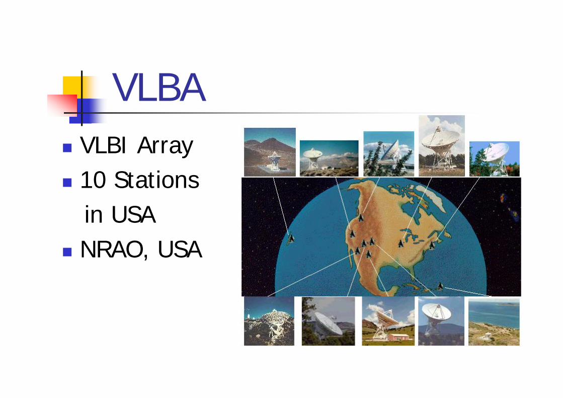
VLBAVLBI Array10 Stationsin USANRAO, USA

VSOPFirst Space VLBI MissionISAS/NAOJ, Japan

VERAJapanese VLBI Array4 Stationsin JapanTwo Beam Differenced ObservationNAOJ

e-VLBIOnline VLBI via High Speed Internet

2. TimeBasic ConceptsIdeal Time Systems

Integrated, Dynamical, BroadcastingPractical Time Scales

Atomic Time, Universal TimeSolar System Barycentric/Coordinate Time

Units and ExpressionJulian Date

Concepts of TimeNewtonian ViewpointAbsolute TimeTime Transformation: 1 to 1Ordering: ChronologyPrecision VS Accuracy

Essential Question on Repeatability

)(τft =

Integrated Time System

Assumption: Constant Duration of A Certain PhenomenonTime = Number of PhenomenaExample

Astronomical: Day, Month, YearMechanical: Pendulum, SpringPhysical: Quartz, Molecule, Atom

Dynamical Time System

Time Argument in Equation of MotionEpoch Determined Inversely from ObservationExample

Mean Longitude of the SunL(T)=Epehemeris Time: ET=T(L)

2089113129602769044841279 T". T". ".' ++

Broadcasting Time System

Time Signals in the Air: JJY, TV, NTTNTP: TS on Computer NetworkGPS Time: TS from GPS Satellites

Standard TimeTime Zone: 15 degree = 1 Hour

Japan Standard Time: JSTJST = UTC + 9 h

Atomic TimeDefinition of SI Second: CGPM (1967)

9192631770 PeriodsSpecific Radiation from Cesium 133

International Atomic Time: TAISteered by BIPM (Paris)Hundreds of Cesium Atomic Clocks+ Several Hydrogen Maser ClocksRelative Precision: 15-16 Digits

Cesium Atomic ClockHP/Agilent 5071A

Atomic Fountain Clock

Hydrogen Maser Clock

Universal TimeDynamical TS based on Earth Rotation

UT = GMT (Greenwich Mean Solar Time)3 Variations: UT0, UT1, UT2Monitored by IERS

UTC (Coordinated Universal Time)Leap Second

Secular Deceleration of Earth Rotation

Solar System Dynamical Time

Official TS of IAU (1984-1991)General Relativistic Effects ConsideredTDB: SS Barycentric Dynamical TimeTDT: Terrestrial Dynamical TimeUnit Adjustment: <TDB> = <TDT>

TDT = TAI+32.184s

Solar System Coordinate TimeOfficial TS of IAU (1991-)

No Unit AdjustmentTCB: SS Barycentric Coordinate TimeTCG: Geocentric Coordinate TimeTT: Terrestrial TimeTT = TDT = TAI+32.184s

TCB-TCG: Time EphemerisHarada and Fukushima (2003)

Time Units1 day=24 hours=1440 min.=86400 sJulian Century: jc, Julian Year: jy

1 jc = 100 jy = 36525 days

Besselian Year = Mean Solar Year = 365.2421897… daysms, μs, ns, ps, fs, …Speed of Light: c = 299792458 m/s

Time ExpressionYear, Month, Day, Hour, Minute, Second

Day of Week, Day of Year

Julian Date: JDJ2000.0 = 12 O’clock, Jan. 1st, 2000= JD2451545.0

Modified Julian Date: MJDMJD = JD – 2400000.5

Julian DateFrom (Y, M, D, h, m, s) to JD

L=int((M-14)/12);I=1461*(Y+4800+L);J=367*(M-2-12*L);K=int((Y+4900+L)/100);N=int(I/4)+int(J/12)-int((3*K)/4)

Julian Date (2)JD0=N+D-32075;JD1=JD0-0.5;JD2=h/24.0+m/1440.0+s/86400.0;JD=JD1+JD2 or JD = (JD1,JD2)

Julian Date (3)From JD to (Y, M, D, h, m, s)

JD0=int(JD-0.5); JD1=JD0-0.5;L=JD0+68569;N=int((4*L)/146097);K=L-int((146097*N+3)/4);I=int(4000*(K+1))/1461001); P=K-int((1461*I)/4)+31;

Julian Date (4)J=int((80*P)/2447);D=P-int((2447*J)/80); Q=int(J/11);M=J+2-12*Q; Y=100*(N-49)+I+Q;JD2=JD-JD1;h=int(JD2*24)m=int(JD2*1440-h*60);s=JD2*86400-h*3600-m*60;

Day of Week

I=JD0-7*int((JD0+1)/7)+2;I: 1,2,3,4,5,6,7I=1: Sunday

3. SpaceSpace Coordinate and UnitSpacial Coordinate Transformation

Rectangular, Spherical, SpheroidalInertial Coordinate System

Parallel Transport of Coordinate Origin, Rotation around Origin

Velocity and Acceleration

Spatial CoordinatesRectangular

Spherical

Spheroidal

),,( zyx

),,( ),,( λφλθ rr

),,( hλϕ

Spherical CoordinateHorizontal

EclipticEquatorialGalactic

)Az,El();Az,Alt();,();,( , AaAzr

δαπ ,,, ,r β λ

,, bπ

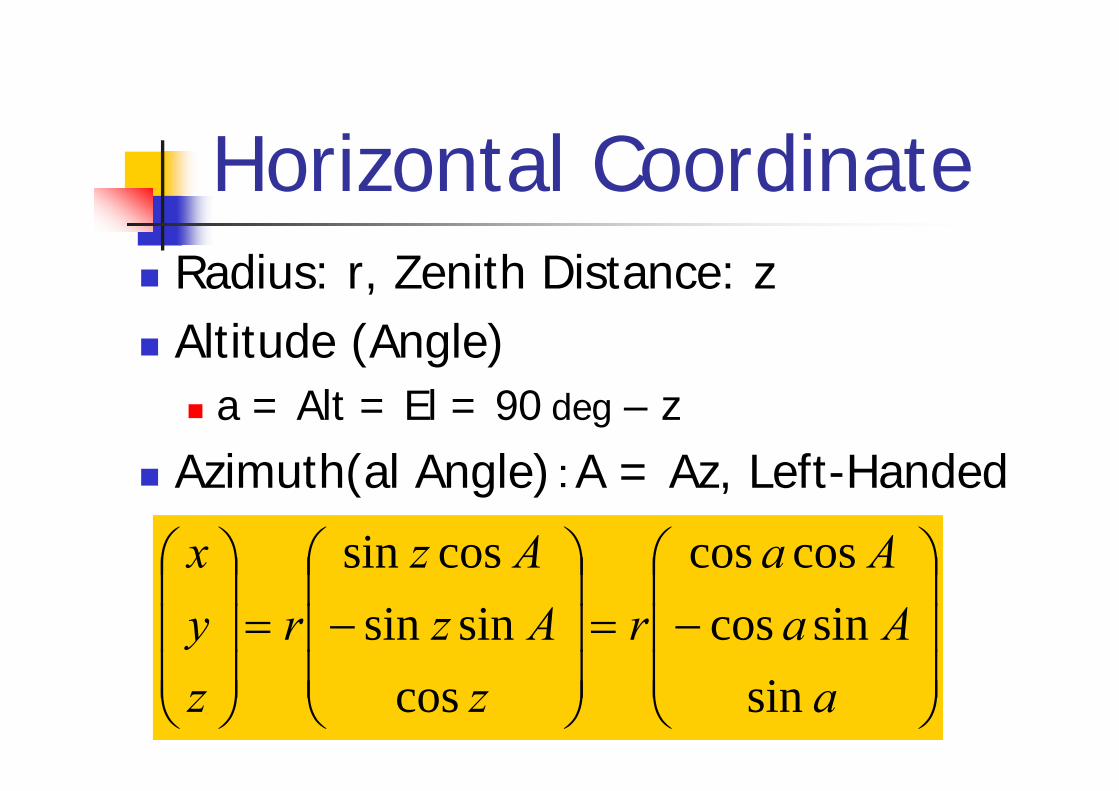
Horizontal CoordinateRadius: r, Zenith Distance: zAltitude (Angle)

a = Alt = El = 90 deg – z

Azimuth(al Angle)：A = Az, Left-Handed

⎟⎟⎟

⎠

⎞

⎜⎜⎜

⎝

⎛−=

⎟⎟⎟

⎠

⎞

⎜⎜⎜

⎝

⎛−=

⎟⎟⎟

⎠

⎞

⎜⎜⎜

⎝

⎛

aAa

Aar

zAz

Azr

zyx

sinsincos

coscos

cossinsin

cossin

Ecliptic CoordinateEcliptic ~ Mean Earth OrbitFor Solar System ObjectsObliquity of Ecliptic: ε

Radius: rLongitude: λLatitude: β

ε

Ecliptic

Equator

Vernal Equinox

Equatorial CoordinateBasic Representation

Right Ascension (R.A.) = αDeclination (Decl.) = δ(Annual) Parallax: π

1 AUsinr

π − ⎛ ⎞= ⎜ ⎟⎝ ⎠

π

AU

r

S

E

P

Angle UnitsRadian: rad

180 deg = π rad

Degree: deg = °Minute of Arc: min = arc minute = 'Second of Arc: second = arc second = " = arcsec = as

Angle Units (2)1 deg = 60 arcmin = 3600 arcsec180 deg = π rad1 arcsec ~ 4.848 μrad

20 arcsec ~ 0.1 mrad: Aberration0.001 arcsec = milli-arcsec: mas0.000001 arcsec = micro-arcsec: μas

Length UnitsSI meter: Defined via SI Second

Speed of Light: c = 299792458 m/s

Astronomical Unit (of Length): AURough: Mean Radius of Earth OrbitRigorous: AU = cτ, τ = 499.00478353… s

Parsec (pc), Light Year (ly)1 pc = AU/sin 1” ~ 30.9 Pm ~ 3.26 ly1 ly = c x 1 jy ~ 9.5 Pm

Spheroidal CoordinateGeographic Latitude: ϕLongitude: λHeight from Reference Ellipsoid: h

cos coscos sin

sin

N

N

Z

xyz

ρ ϕ λρ ϕ λ

ρ ϕ

⎛ ⎞ ⎛ ⎞⎜ ⎟ ⎜ ⎟=⎜ ⎟ ⎜ ⎟⎜ ⎟ ⎜ ⎟⎝ ⎠ ⎝ ⎠

Geographic LatitudeGeocentric Latitude: φGeographic/Geodetic Latitude: ϕ

φ ϕEquator

PoleP

r

Geocenter H

Zenith

Nadir

Horizon

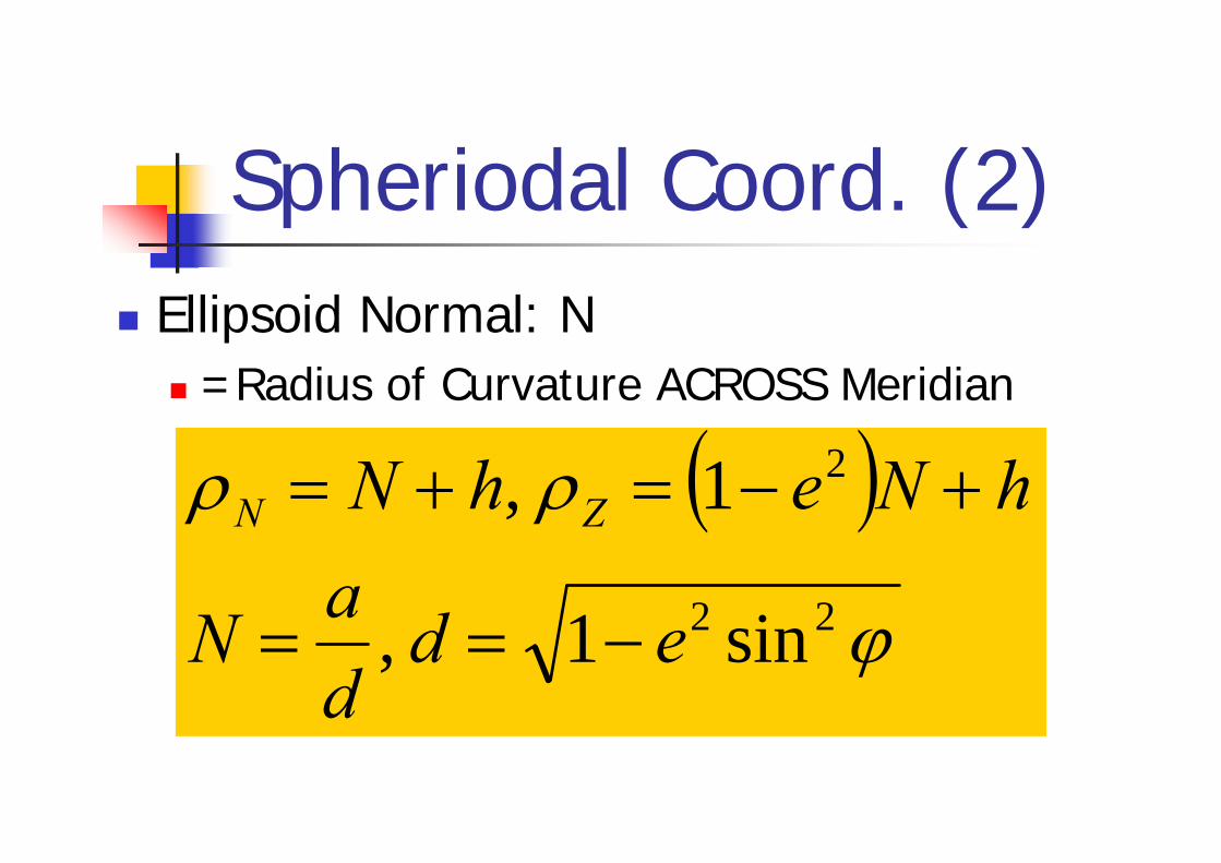
Spheriodal Coord. (2)Ellipsoid Normal: N

=Radius of Curvature ACROSS Meridian

( )ϕ

ρρ

22

2

sin1 ,

1 ,

eddaN

hNehN ZN

−==

+−=+=

EllipseSemi-Major Axis: aSemi-Minor Axis: b

12

2

2

2

2

2

=++bz

ay

ax

a

b

Flattening FactorFlattening Factor: fEccentricity: e, Complimentary Ecc.: ec

2

2 22 2

2

, 1 1

2

ca b bf e e f

a aa be f f

a

−≡ ≡ = − = −

−≡ = −

Spherical to Rectangular

sin cos cos cossin sin cos sin

cos sin

xy r rz

θ λ φ λθ λ φ λθ φ

⎛ ⎞ ⎛ ⎞ ⎛ ⎞⎜ ⎟ ⎜ ⎟ ⎜ ⎟= =⎜ ⎟ ⎜ ⎟ ⎜ ⎟⎜ ⎟ ⎜ ⎟ ⎜ ⎟⎝ ⎠ ⎝ ⎠ ⎝ ⎠

Rectangular to Spherical

),atan2

),,atan2sin

),,atan2cos

,

1

1

22222

x(y

p(zrz

z(prz

yxpzyxr

=

=⎟⎠⎞

⎜⎝⎛=

=⎟⎠⎞

⎜⎝⎛=

+=++=

−

−

λ

φ

θ

Spheroidal to Rectangular

cos coscos sin

sin

N

N

Z

xyz

ρ ϕ λρ ϕ λ

ρ ϕ

⎛ ⎞ ⎛ ⎞⎜ ⎟ ⎜ ⎟=⎜ ⎟ ⎜ ⎟⎜ ⎟ ⎜ ⎟⎝ ⎠ ⎝ ⎠

( )ϕ

ρρ

22

2

sin1 ,

1 ,

eddaN

hNehN ZN

−==

+−=+=

Rectangular to Spheroidal

Difficult Inverse ProblemEasy: LongitudeEliminating Longitude

-> Latitude Equation

),atan2 x(y=λ

( )( )( )

2 2

2

cos

1 sin

N h p x y

N e h z

ϕ

ϕ

⎧ + = ≡ +⎪⎨

− + =⎪⎩

Latitude EquationAfter Elimination of h

2 2

2

sin cossin cos1 sin

where

Cp ze

C ae

ϕ ϕϕ ϕϕ

− =−

=

Latitude Equation (2)Variable TransformationTransformed EquationDerivation and Solution

cott ϕ=

2

2

( ) 0

where 1

Ctf t zt pg t

g e

≡ + − =+

≡ −

Derivation of Lat. Eq.

( )

2 2

2 2 2 22

2

2 2

1sin ,cos1 1

111 1 1 11

1

1

tt t

p zt C tt t t te

tCtp zte t

ϕ ϕ= =+ +

∴ − =+ + + +−

+

− =− +

Solution of Lat. Eq.

(0) 0, ( ) 00

f p f zt Ct= − ≤ +∞ ≈ + ≥

∴ ≤ ≤ +∞

Localization (Northern Hemisphere)Variable Domain after Localization

Newton MethodInitial Guess 0 /

ptz C g

=+

z≤0

Newton MethodEffective to Solve Nonlinear Eq.

EssenceLinearization

Newton Iteration

0)( =xf

)(')()(*

xfxfxxf −≡)(* xfx →

y=f(x)

xx0 x1x

y

Newton Method (2)Quadratic Convergence

Doubling Effective DigitsFast but UnstableSlow when Multiple RootsKey Points

Bracketing to Assure UniquenessSelecting Stable Starters

Stable StarterBracketing

Assumption 1

Assumption 2

Stable Starter: Upper Bound of Solution

RL xxx <<

( ) ( )RL xfxf << 0

0)('',0)(' >>→<< xfxfxxx RL

Application to Lat. Eq.Preparation

( )

( )

( )

2

32

52

( )

( 0 ) 0

'( ) 0

3''( ) 0

C tf t z t pg t

f p fC gf t z

g t

C g tf tg t

≡ + −+

= − ≤ ≤ + ∞

= + >+

−= <

+

Application (2)Newton Iteration

Stable Starter: Lower Bound of Solution*

0 0 (0)/

pt fz C g

= → =+

( )( )

32 3

*3

2

( )( )'( )

p g t Ctf tf t tf t z g t Cg

+ −≡ − =

+ +

Velocity & AccelerationVelocity = Variation of PositionAcceleration = Variation of VelocityJerk = Variation of Acceleration

2 3

2 3

d d d, , dt dt dt

= = =x x xv a j

Velocity in Spherical CS

d d d ddt dt dt dt

r r

rr

v v vφ φ λ λ

φ λφ λ

⎛ ⎞∂ ∂ ∂⎛ ⎞ ⎛ ⎞= = + +⎜ ⎟ ⎜ ⎟⎜ ⎟∂ ∂ ∂⎝ ⎠ ⎝ ⎠⎝ ⎠= + +

x x x xv

e e e

d d d, , cosdt dt dtrrv v r v rφ λ

φ λφ= = =

Vector Representation

Component Representation

Coordinate Triad in Spherical CS

⎟⎟⎟

⎠

⎞

⎜⎜⎜

⎝

⎛=⎟

⎠⎞

⎜⎝⎛∂∂

≡φλφλφ

sinsincoscoscos

rrxe

⎟⎟⎟

⎠

⎞

⎜⎜⎜

⎝

⎛−−

=⎟⎟⎠

⎞⎜⎜⎝

⎛∂∂

≡φ

λφλφ

φφ

cossinsincossin

1 xer

⎟⎟⎟

⎠

⎞

⎜⎜⎜

⎝

⎛−=⎟

⎠⎞

⎜⎝⎛∂∂

≡0

cossin

cos1 λ

λ

λφλxe

r

Velocity in SpheroidalCS

d d ddt dt dt h hh v v v

h ϕ ϕ λ λϕ λ

ϕ λ⎛ ⎞∂ ∂ ∂⎛ ⎞ ⎛ ⎞= + + = + +⎜ ⎟ ⎜ ⎟⎜ ⎟∂ ∂ ∂⎝ ⎠ ⎝ ⎠⎝ ⎠

x x xv e e e

( )( )

2

32 2

d d d, , cosdt dt dt

1,

1 sin

h M N

M

hv v v

a eM h M

e

ϕ λϕ λρ ρ ϕ

ρϕ

= = =

−= + =

−

Vector Representation

Component Representation

Coordinate Triad in Spheroidal CS

⎟⎟⎟

⎠

⎞

⎜⎜⎜

⎝

⎛=⎟

⎠⎞

⎜⎝⎛∂∂

≡ϕ

λϕλϕ

sinsincoscoscos

hhxe

⎟⎟⎟

⎠

⎞

⎜⎜⎜

⎝

⎛−−

=⎟⎟⎠

⎞⎜⎜⎝

⎛∂∂

≡ϕ

λϕλϕ

ϕρϕ

cossinsincossin

1 xeM

⎟⎟⎟

⎠

⎞

⎜⎜⎜

⎝

⎛−=⎟

⎠⎞

⎜⎝⎛∂∂

≡0

cossin

cos1 λ

λ

λϕρλxe

N

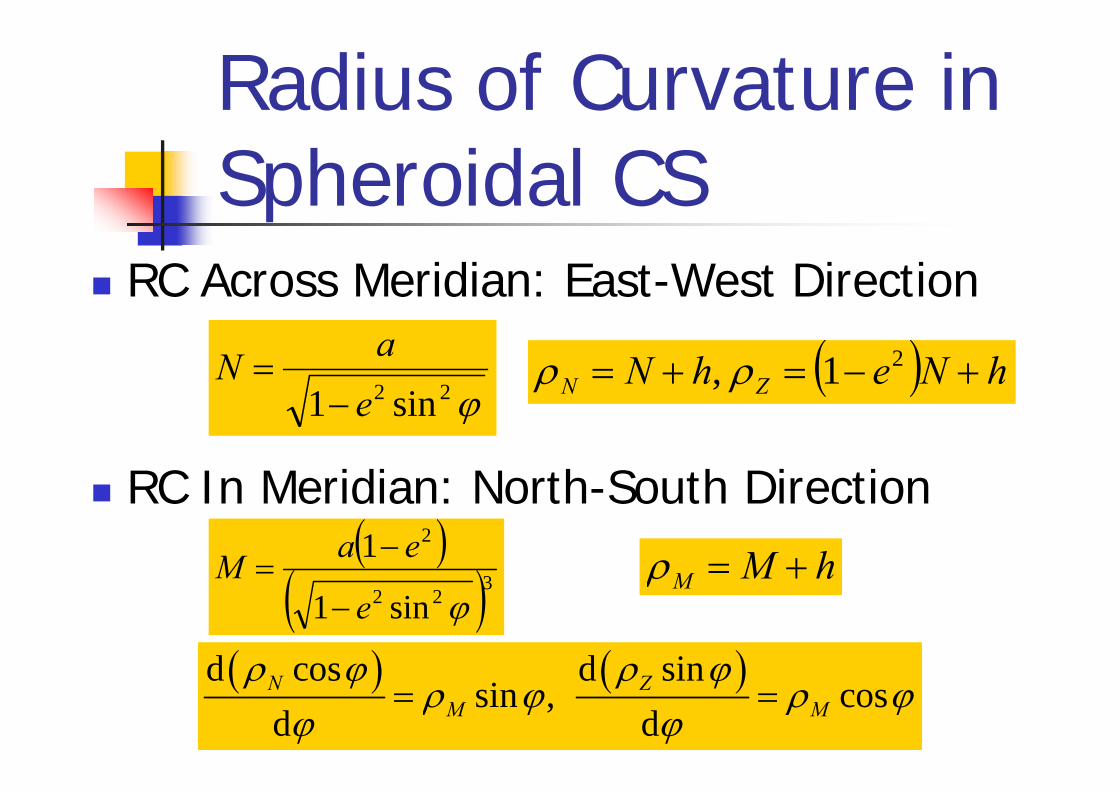
Radius of Curvature in Spheroidal CS

RC Across Meridian: East-West Direction

RC In Meridian: North-South Direction( )

( )322

2

sin1

1

ϕe

eaM−

−=

ϕ22 sin1 eaN

−=

( ) ( )d cos d sinsin , cos

d dN Z

M M

ρ ϕ ρ ϕρ ϕ ρ ϕ

ϕ ϕ= =

( ) hNehN ZN +−=+= 21 , ρρ

hMM +=ρ

Inertial Coordinate System

CS where Law of Inertia HoldsNewton’s Law of Inertia

No Force -> Linear Motion

Galilei’s Principle of RelativityLaw of Physics is Invariant at Any ICS

Parallel Transport of Coordinate OriginICS to ICS

Parallel Transport of Coordinate Origin

Galactic Center in Quasar-Rest FrameCosmic Expansion

Local Standard of Rest in Galactic CSLocal Standard of Rest (LSR) = Solar System BarycenterFeature of Local Motion: Oort’s Constant

Parallel Transport of Coordinate Origin (2)

Geocenter in Solar System Barycentric CSPlanetary Ephemeris

Averaged Crust in Geocentric CSEarth Rotation

Observer in Terrestrial CSFixed to Earth Surface (= Averaged Crust)Surface Motion (Aircraft, Ship, Car, etc)

Ephemeris and AlmanacNumerical Table on Complicated Motion

Orbit: Planets, Satellites, AsteroidsRotation: Planets, Satellites

Astronomical Almanac (US+UK)Japanese EphemerisNASA/JPL DE series, DE413/408

Most Precise, Machine Callable

Spatial Coordinate Transformation

General Transf.

Taylor Expansion w.r.t. New Coordinates

( )txXXx kjjk ,=←

( ) ( )

( ) ( ) ++=

+∂

∂+=

∑

∑

=

=

kk

jkj

kk k

jjj

xtBtA

xtxX

tXX

3

1

3

1,0,0

Linear Transformation

( ) ( )xAX tt B+=General Affine Transformation

Static: 12-Parameter Transformation

xAX B+=

Coefficient MatrixΘ++= SDB

Scaling: Diagonal Component

Shear: Non-Diagonal, Symmetric

Infinitesimal Rotation: Asymmetric

kjjk ≠= if 0D

( )S S S 0 if jk kj jk j k= = =

kjjk Θ−=Θ

7-Parameter Transformation

CT between Similar Two CSIsotropic ScalingOrigin ShiftRotation

Ex.: Transf. among Geocentric CSsWorld Geod. System (ITRFnn, GRS80)Tokyo Datum and JGD 2000

( )xXX Θ++= Is0

5. Motion of Celestial Bodies

Rest: QuasarLinear: Most of StarsRotation: Earth, the Moon, SatelliteKepler: BinariesQuasi-Kepler: Asteroid, SatelliteComplicated: Planet, Space Vehicle

Resting BodyQuasar: Practically Being RestPosition Expression

EpochMean Place at EpochParallax at Epoch

Quasar Catalogs: IAU, ICRFnn

0t( )00 ,δα

0π

Linear Motion

Different Treatment for Radial Comp.Proper Motion = Linear Motion on Celestial Sphere

( ) ( )000 ttt −+= vxx

⎟⎟⎟

⎠

⎞

⎜⎜⎜

⎝

⎛=

δαδαδ

sinsincoscoscos

rx ( )0

0

0

0

ttVrr R

−⎟⎟⎟

⎠

⎞

⎜⎜⎜

⎝

⎛+⎟⎟⎟

⎠

⎞

⎜⎜⎜

⎝

⎛≅

⎟⎟⎟

⎠

⎞

⎜⎜⎜

⎝

⎛

δ

α

μμ

δα

δα

Star CatalogEpoch, Mean Place, and ParallaxPropor MotionRadial VelocityAstrophysical Information

Luminosity, Color, Variability, etc.Astrometric Star Catalogs

HIPPARCOS, FKn, PPM, AGKn

( )δα μμ ,

RV

6. RotationRotation = Orthogonal Transformation

Infinitesimal Rotation: Vector ProductFinite Rotation: Orthogonal Matrix

Euler’s TheoremFundamental RotationAngular Velocity

OrthogonalTransformation

Distance Invariant in Euclidean Space

Rotation: A Linear Transformation

Orthogonality

( ) ( )22 xX Δ=Δ

xX Δ=Δ R

( ) ( )TT

T

RRIRRRRR==∴

Δ=ΔΔ=Δ1

2T2

or -

xxxx

Finite Rotation

Expression: Matrix, Spinor, QuarternionRotational Operation: Matrix ProductRotation Matrix = Coordinate Triad

= Trio of Orthonormal Basis

( )TX Y Z= e e eRX

YZ

Euler’s Theorem

Any Finite Rotation = Triple Product of Fundamental Rotation Matrices

Euler Angles = 3 Fundamental Rotation Angles

( ) )()()(,, αβγγβα ijkijk RRRRR ≡=

( )( ) ( )αβγγβα −−−=− ,,,, 1kjiijk RR

Fundamental Rotation OperationRotate around z-axis by the angle θ

)()(3 θθ zRR =

θ X

Y

xy P

Fundamental Rotation Operation (2)

Rotation Around j-th Axis by θ

Reverse Rotation

)(θjR

( )( ) ( )θθ −=−jj RR 1

Fundamental Rotation Matrix

Ex.: Ecliptic-Equatorial Transf. Obliquity of Ecliptic

⎟⎟⎟

⎠

⎞

⎜⎜⎜

⎝

⎛−=

1000cossin0sincos

)(3 θθθθ

θR

( )ε1Rε

Fundamental Rotation Matrix (2)Small Angle Approximation

( )

( ) ×⎟⎟⎠

⎞⎜⎜⎝

⎛−≅∴

×−=⎟⎟⎟

⎠

⎞

⎜⎜⎜

⎝

⎛−+≅

∑∏j

jjj

jj e

e

θθ

θθθ

θ

IR

IIR 33 0000000

Euler RotationCombinations of Euler Angles: 3x2x2=123-1-3 (=X) Convention

Most Popular, the Euler AnglesUsed in Classic Rotational Dynamics

( ) ( ) ( ) ( )ψθφφθψ 313313 ,, RRRR =

3-1-3 Rotation Matrix

( )⎟⎟⎟

⎠

⎞

⎜⎜⎜

⎝

⎛

−+−−−+−

=

θφθφθ

θψφθψφψφθψφψ

θψφθψφψφθψφψ

φθψCCSSS

SCCCCSSSCCCSSSCCSSCSCSCC

,,313R

⎟⎟⎟

⎠

⎞

⎜⎜⎜

⎝

⎛

−+−−−+−

=θφθφθθψφθψφψφθψφψθψφθψφψφθψφψ

coscossinsinsinsincoscoscoscossinsinsincoscoscossinsinsincoscossinsincossincossincoscos

3-1-3 Euler Angles

X

Z

YN

P

ψ

θ

φ

Weak Point of 3-1-3 Convention

( ) ×⎟⎟⎟

⎠

⎞

⎜⎜⎜

⎝

⎛

+−≅

ψφ

θφθψ 0,,313 IR

Degeneracy in Small Angles

RecipeUse 3-2-1 and Other Convention with All Different Indices

3-2-3 ConventionAlias: Y-Convention, Ex.: Precession

Screw: Rotation Around Fixed Direction

⎟⎟⎟

⎠

⎞

⎜⎜⎜

⎝

⎛=

ϕλϕλϕ

cossinsincossin

n

( ) ( ) ( )323 , , I+ sin 1 cosλ ϕ χ χ χ= ×+ − × ×n n nR

( )AAA z−−= ,,323 θζRP

Other Conventions1-3-1: Nutation

2-1-3: Polar Motion + Sidereal Rotation

1-2-3: Aerodynamics, Attitude ControlOne of Most Desirable Conventions

( )( )εεψε Δ+−Δ−= AA ,,131RN

( )pp xy −−Θ= ,,312RWS

Rotation and Velocity Transformation

= ⇒

= +

= −Ω= − ×

X x

V v x

v xv ω x

RdRRdt

RR

Angular Velocity

( )

dddt dt

j j j jjj

jj

j

θ θ

θ

⎛ ⎞= ≅ − ×⎜ ⎟

⎝ ⎠⎡ ⎤⎛ ⎞

= − × = − × = −Ω⎢ ⎥⎜ ⎟⎝ ⎠⎣ ⎦

∑∏

∑

e

e ω

∵R R I

R

ddt

jj

j

θ=∑ω e

Infinitesimal Rotation3D Anti-Symmetric Matrix ~ Axial Vector

True Meaning of Vector Product

xθx Δ×=ΘΔ

⎟⎟⎟

⎠

⎞

⎜⎜⎜

⎝

⎛

−−

−=Θ

00

0

xy

xz

yz

θθθθθθ

⎟⎟⎟

⎠

⎞

⎜⎜⎜

⎝

⎛=

z

y

x

θθθ

θ

Small Angle Rotation( )

×⎟⎟⎟

⎠

⎞

⎜⎜⎜

⎝

⎛−≅

⎟⎟⎟

⎠

⎞

⎜⎜⎜

⎝

⎛

−++−−+−+

=

=

γβα

αβγγβα

αβαββ

αγαβγαγαβγβγ

αγαβγαγαβγβγ

I

RRRR

CCSCSSCCSSCCSSSCSSSCSCCSSSCCC

)()()(,, 123123

7. Earth RotationBase of Coordinate Transformation between Geocentric and Terrestrial Coordinate SystemSidereal Rotation (S) … Rotation Angle UT1Motion of Figure Axis

Quasi-Diurnal: Polar Motion = Wobble (W)Others: Precession (P) + Nutation (N)

Matrix Representation

WSNPR =

Precession + NutationFigure Axis Motion (Other than Wobble)2 Components in Ecliptic CS

Longitude, ObliquityPrecession=Very Long Periodic Motion

50 arcsec/y, ~26000y PeriodNutation=Other Periodic Motion

18.6y, 0.5y, 9.3y, etcNew Model Soon Appears

Ecliptic

Ecliptic Pole

z

PrecessionDiscovery: Hipparchus (~150BC)Old Model: IAU1976

Lieske et al. (1976, A&A)Dynamics: Newcomb’s TheoryCorrection of Planetary MassesAdding Geodesic Precession

Theory: in Ecliptic CSFormula: in Equatorial CS

Precession (2)

3 Precession Angles in Equatorial CS

Unit: 1 arcsecT =(JD-2451545.0)/36525

( )AAA z−−= ,,323 θζRP

32

018203.0041833.0

017998.0

09468.142665.0

30188.0

2181.23063109.20042181.2306

TTTzA

A

A

⎟⎟⎟

⎠

⎞

⎜⎜⎜

⎝

⎛−+

⎟⎟⎟

⎠

⎞

⎜⎜⎜

⎝

⎛−+

⎟⎟⎟

⎠

⎞

⎜⎜⎜

⎝

⎛=

⎟⎟⎟

⎠

⎞

⎜⎜⎜

⎝

⎛θζ

Precession (3)Approximation of Precession Matrix

Correction in R.A. and Decl.

⎟⎟⎟

⎠

⎞

⎜⎜⎜

⎝

⎛ −−≅

1001

1

A

A

AA

θφ

θφP AAA z+≡ζφ

tan sin , cosP A A P Aα φ θ δ α δ θ αΔ = + Δ =

Precession (4)Approximation of Precession Angle

Precession (Speed) in R.A. and Decl.

Approximate Correction Formula

TnTm PAPA ≅≅ θφ ,

/jy"3109".2004 ,/jy"4362.4612 == PP nm

( )( )Tn

Tnm

PP

PPP

αδαδα

cos ,sintan

≅Δ+≅Δ

NutationDiscovery: Bradley (1747)Old Model: IAU1980

Seidelmann et al. (1981, CM)Rigid Earth: Kinoshita (1977, CM)Non-Rigidity: Wahr (1981, GJRAS)

Mean Obliquity (Lieske et al., 1976)

32 001813".000059".0

8150".46448".21'2623

TT

TA

+−

−°=ε

Nutation (2)

( )( )εεψε Δ+−Δ−= AA ,,131RNMatrix Representation

Nutation in Longitude ΔψNutation in Obliquity ΔεAnalytic Expression

∑∑=

=⎟⎟⎠

⎞⎜⎜⎝

⎛=⎟⎟

⎠

⎞⎜⎜⎝

⎛ΔΔ 5

1

,cossin

jjjk

k kk

kk ΩnAAA

εψ

εψ

Delauney AnglesMain 5 Angles in Nutation Theory

Mean Anomaly of MoonMean Anomaly of SunMean Argument of Latitude of MoonMean ElongationMean Longitude of Ascending Node of Moon

Details: Seidelmann et al. (1981)

'F

'LLD −≡

Ω

Rough Approx. of NutationPrecision: 0.1 arcsecUnit: 1 arcsec

+⎟⎟⎠

⎞⎜⎜⎝

⎛+⎟⎟⎠

⎞⎜⎜⎝

⎛+⎟⎟⎠

⎞⎜⎜⎝

⎛−+

⎟⎟⎠

⎞⎜⎜⎝

⎛−

+⎟⎟⎠

⎞⎜⎜⎝

⎛−+⎟⎟⎠

⎞⎜⎜⎝

⎛−=⎟⎟

⎠

⎞⎜⎜⎝

⎛ΔΔ

0sin1.0

0'sin1.0

2cos1.02sin2.0

2cos1.02sin2.0

'2cos6.0'2sin3.1

cos2.9sin2.17

LL

ΩΩ

LL

ΩΩ

εψ

Approx. NutationApproximation of Nutation Matrix

Nutation in R.A. and Decl.

⎟⎟⎟

⎠

⎞

⎜⎜⎜

⎝

⎛

ΔΔΔ−ΔΔ−Δ−

≅1

11

ενεμνμ

N

AA εψνεψμ sin,cos Δ=ΔΔ=Δ

Approx. Nutation (2)Correction in R.A. and Decl.

( )αεανδ

αεανδμαsincos

,cossintanΔ+Δ=Δ

Δ−Δ+Δ=Δ

N

N

Sidereal Rotation

( )3= ΘS R

Almost Uniform Quasi-Diurnal RotationΩ0 = 7.2921150(1) x 10-5 radian/s

Angular Rotation = 360 degree/Sidereal Day ~ 365.2422.../366.2422... Rot./DayGreenwich Apparent Sidereal Time (GAST) Θ

Deviation from Uniform Rotation

UTC → UT1 → GMST → GASTDUT1 = UT1-UTC: UnpredictableGMST = GMST0 + r UT1 + ...Ratio of Sidereal/Universal Time: rr ~ 1.0027379... GAST = GMST + Δψ cos ε + ...

Length of Day (LOD) = 2π/Ω

Polar Motion = Wobble

( ) ( )2 1p px y= − −W R R

Slow Motion of Pole Viewed on EarthSymbol: (xp, yp), Size: 0.1 arcsec ~ 30mPeriods: Annual, Chandler (~14 month)

Unpredictable = To be Monitored

EOPEarth Orientation Parameters

DUT1, LOD, xp, yp,, Pole OffsetsOld Terms: Earth Rotation Parameters (ERP)

Pole Offset = Error in Prec./Nut. TheoryInternational Earth Rotation Service (IERS)

Since 1984, Joint Service of IAU and IUGGHomepage: http://www.iers.org/

8. Keplerian MotionSolution of Two-Body ProblemGravitational Constant

Orbital Element = 6 ConstantsShape of OrbitOrientation of Orbital PlaneLocation in Orbit

xx32

2

rdtd μ−

=( )mMG +=μ

ea,ω,, IΩ

T

Unit of MassSI Unit of Mass: kgAstronomical Unit: Solar MassUniversal Constant of Gravitation: GObservable = GM = Gravitational Constant of Central Body

Heliocentric GC = Sun’s GMGeocentric GC = Earth’s GM

SGM

EGM

SM

Orbital ElementsSemi-Major Axis: aOrbital Eccentricity: eLongitude of Ascending Node: ΩOrbital Inclination: IArgument of Pericenter: ωTime of Pericenter Passage: T

EllipseSemi-Major Axis: aSemi-Minor Axis: b

12

2

2

2

=+by

ax

a

b

Orbital EccentricityEccentricity: e, Complimentary Ecc.: e’

22

22

1' , eabe

abae −=≡

−≡

ae

F

Orbital Plane3-1-3 Euler Angles of Orbital Plane

3 Important Direction VectorsOrigin of Longitude: X-axisAscending Node: NPericenter: P

( ) ( ) ( ) ( )Ω=Ω 313313 ,, RRRR II ωω

Z

P

γ

NΩ

I

ω

Orbital Plane (2)

Keplerian OrbitElliptical: e < 1

Planet, Satellite, BinaryParabola: e = 1

Good Approximation of Comet OrbitQuasi-Parabola: e ~ 1

Comet, Peculiar AsteroidsHyperbolic: e > 1

Space Vehicle, Close Encounter

Element to Position and Velocity (Elliptic)

Solve (Elliptic) Kepler’s Equation

Speed of Ecc. Anomaly EPV in Orbital Plane

( )⎩⎨⎧

=−=Eb

eEasin

cosη

ξ

( )TtnEeE −=− sin

EenEcos1−

=

⎩⎨⎧

=−=

EEbEEa

cossin

ηξ

Element to Position and Velocity (Parabolic)

Solve Barker’s Eq. = Parabolic Kepler’s Eq.

Speed of τPV in Orbital Plane

( )21

2

q

q

ξ τ

η τ

⎧ = −⎪⎨

=⎪⎩

( )3

33 2t T

qτ μτ + = −

2 3

11 2q

μττ

=+

22

qq

ξ ττη τ

⎧ = −⎨

=⎩

Element to Position and Velocity (Hyperbolic)

Solve (Hyperbolic) Kepler’s Equation

Speed of FPV in Orbital Plane

( )coshsinh

a e Fb F

ξη

⎧ = −⎨

=⎩

( )sinhe F F n t T− = −

cosh 1nF

e F=

−

sinhcosh

aF FbF F

ξη

⎧ = −⎨

=⎩

Element to PV (2)Reverse Euler Rotation

( ) ( )⎟⎟⎟

⎠

⎞

⎜⎜⎜

⎝

⎛

−−−=00

,, ηξ

ηξ

ω ΩI, 313Rvx

Kepler’s EquationFirst Transcendenal Equation in HistoryElliptic

Parabolic

Hyperbolic

MEeE =− sin

PM=+3

3ττ

HMFFe =−sinh

Elliptic Kepler’s Eq.Eccentric Anomaly: E Mean Anomaly: MKepler’s 3rd LawTrue Anomaly: f

MEeE =− sin

( )⎩⎨⎧

===−=

frEbfreEa

sinsincoscos

ηξ

32an=μ

( )M n t T= −

Solution of Kepler’s Eq.

Domain Reduction

Newton Method

( )

( ) ( )( )

( )

*

* cos sin' 1 cos

E f E

f E M e E E Ef E E

f E e E

→

− −≡ − =

−

( ) 0sin =−−≡ MEeEEf

0 0M M Eπ π−∞ < < ∞⇒ ≤ < ⇒ ≤ <

Stable Starter of Newton Merthod

Stability Theory ofNewton MethodUpper Bound as Stable StarterExamples

( ) ( )( ) ( ) 0'',0'

,00>>

<≤EfEf

ff π

( ) ( )

⎟⎠⎞

⎜⎝⎛

++

+−

=

⎟⎟⎠

⎞⎜⎜⎝

⎛⎟⎠⎞

⎜⎝⎛=

eeMeM

eM

fffE

1 ,,

1min

,2

,0min ***0

π

ππ

( )0* Ef

Perturbed KeplerianOrbit

Element = Slow Function of Time

Perturbation TheoryPolynomials + Fourier Series

( ) ( )tΛTΩIeaΛ =≡ ,,,,, ω

( )∑ ++

+++=

kkkkk tStC

tΛtΛΛΛνν sincos

2210

Complicated OrbitEq. of MotionSolution

Numerical: Numerical IntegrationAnalytical: Perturbation Theory

Parameters Estimation by Fitting Solution to Obs. DataResult: Astronomical Ephemeris

+−

= xx32

2

rdtd μ

Astronomical EphemerisNumerical: DE (NASA/JPL, USA)Analytical: VSOP/ELP (BdL, France)DE: Available through NAOJ/ADAC

Software (Fortran/C) + Binary FilesDE408: BC10000-AD10000, UNIX/Win/MacPV of Sun, Moon, and 9 Major Planets

Whole Solar System Bodies: HORIZONShttp://ssd.jpl.nasa.gov/

9. Signal PropagationGeometric Optics ApproximationBasic: One-way PropagationApplication: Multi-way Prop.Light Direction: Aberration & ParallaxDoppler ShiftPropagation Delay

One-Way PropagationPhoton: Linear Motion

Constant Speed of LightSpecial Theory of Relativity

( ) ( )000 ttt −+= VXX

c=0V

Source

Observer

t = t0

t = t1

Photon

Passive ObservablesArrival Epoch

Incoming Direction

Observed Wavelength

1t

1d

1λ

Eq. of Light TimeWithin Solar SystemDeparture EpochArrival EpochLight Time = Duration

Equation to Solve LT ( )10c Rτ τ=

S

O

01 tt −≡τ

0t1t

Eq. of Light Time (2)Diff. in Departure/Arrival Position

( )1 0 1 0t t− = −x x V

Evaluate Magnitude of Diff. Vector

Assume that Source/Observer Motions are Known

10R Vτ=

( ) ( )tt OS xx ,

Eq. of Light Time (3)

V c=

( ) ( ) ( ) ( )( ) ( ) ( ) ( )

0 0 1 1 10 10

10 1 0 1 1

, , ,S O

O S S

t t R

t t t

τ τ

τ τ

= = ≡

= − = − −

x x x x R

R x x x x

Use Constant Speed of Light

Final: Equation of Light Time

( )10c Rτ τ=

Eq. of Light Time (4)

Newton Method

Correction Formula

( ) ( ) 0f c Rτ τ τ≡ − =

( )*fτ τ→

( ) ( )( )

( ) ( )( )

* '' '

f R Rf

f c Rτ τ τ τ

τ ττ τ

−′ ≡ − =−

Eq. of Light Time (5)Initial Guess: Infinite Speed of LightOne Newton Correction

Next Stage: General Relativity Needed

( ) ( )1 * 0 SO

SO

Rfc V

τ ≡ =−

( ) ( )( ) ( )( )1 1 1 11 1 , S S

SO S SOSO

t tR t V

R− ⋅ −

= − =v v x x

x x

Light Direction

Aberration: Effect of Observer’s VelocityParallax: Effect of Observer’s PositionPeriods: Annual, Diurnal, Monthly, etc. Correction for Light Time: MUST within Solar System

101

1 10R−−

= =RVd

V

AberrationBradley (1727)Finiteness of Speed of Light

Ex.: Raindrops Trails on Side WindowVector Expression of Aberration

( ) ( )1 1

1 1

' cc c

− − − ⋅+= = ≈ +

− +1 1 1

1

V v v d v dd vd dV v d v

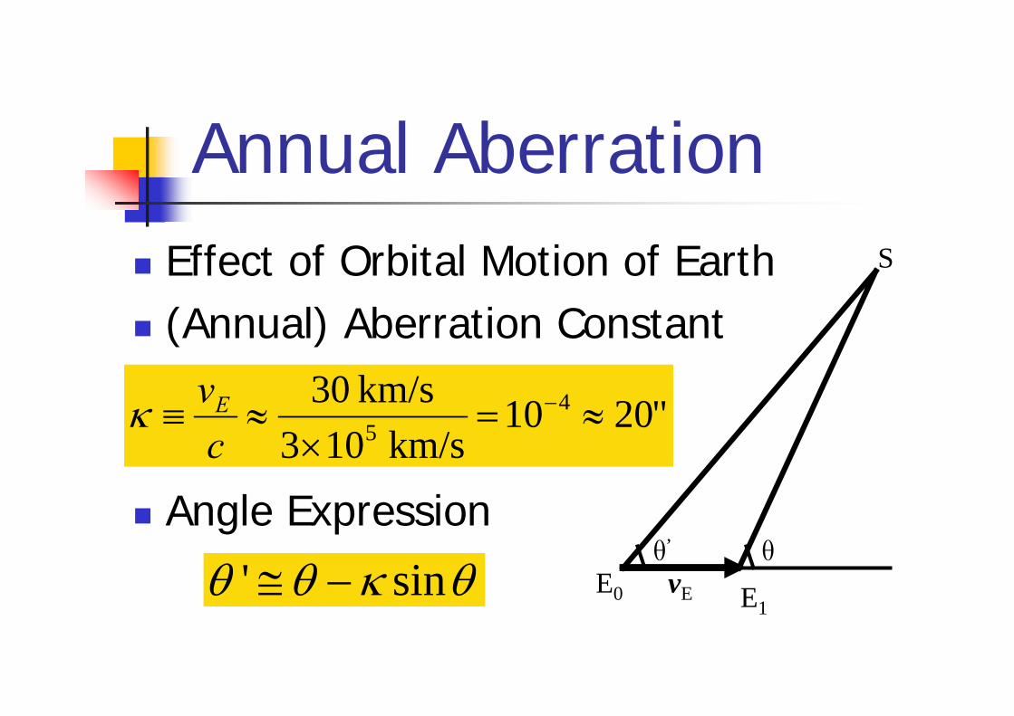
Annual AberrationEffect of Orbital Motion of Earth(Annual) Aberration Constant

Angle Expression

"2010km/s 103

km/s 30 45 ≈=

×≈≡ −

cvEκ

' sinθ θ κ θ≅ −

S

E0

θ’

E1

θvE

Annual Aberration (2)Ecliptic Coordinate System is UsefulApproximation Formula

Mean Longitude of Sun: LAberration Ellipse

( )( ) ( )⎩⎨⎧

−−≈Δ−≈Δ

λκλβλβκβ

LL

A

A

coscossinsin

( ) 1sin

cos22

=⎟⎟⎠

⎞⎜⎜⎝

⎛ Δ+⎟

⎠⎞

⎜⎝⎛ Δ

βκβ

κλβ AA

Diurnal AberrationEffect of Earth RotationEquatorial CS is UsefulDiurnal Aberration Constant

Approx.Formula

Sidereal Rotation Angle: Θ, Geoc. Lat.: φ

( )( ) ( )⎩⎨⎧

−Θ−≈Δ−Θ≈Δ

αφκαδαδφκδ

coscos''cossinsincos''

A

A

"3.0106.1m/s103

m/s480' 68 ≈×=

×≈≡ −

cR EEωκ

ParallaxBessel (1838): 81 CygniDeviation of Observer’s Position from its Mean Value

Ex.: Direction Difference between Right/Left Eye’s View

Vector Expression of Parallax( )1 0 1 00 1 0 1 0

00 1 0 1 0 0

rR r r

− ⋅− −= = = ≈ −

− −x d x dx x d xRd d

x x d x

Annual ParallaxEffect of Earth Orbital MotionAlternative Distance Measure

Angle Expression0

AU 1r

≈π

00 sinθπθθ +≈Sun E

S

θ0 θ

Annual Parallax (2)Approximation Formula in Ecliptic CS

Note: 90 deg Phase Diff. from AberrationParallactic Ellipse

( )( ) ( )⎩⎨⎧

−≈Δ−≈Δ

00

00

sincoscossin

λπλβλβπβ

π

π

LL

( ) 1sin

cos2

0

20 =⎟⎟

⎠

⎞⎜⎜⎝

⎛ Δ+⎟

⎠⎞

⎜⎝⎛ Δ

βπβ

πλβ ππ

Diurnal ParallaxEffect of Earth Radius: Moon, Artificial Sat.Approximation Formula in Equatorial CS

Yet Another Distance Measure: Horizontal Parallax

( )( ) ( )⎩⎨⎧

−Θ≈Δ−Θ≈Δαφπαδαδφπδ

π

π

sincos''coscossincos''

πππ 51 104AU1

sin' −− ×≈⎟⎠⎞

⎜⎝⎛≈⎟

⎠⎞

⎜⎝⎛≡ EE R

rR

Doppler ShiftClassic (= Non-Relativistic) Approximation

Outgoing Object = Red ShiftIncoming Object = Blue Shift

( )c

z dvv ⋅−=

−≡ 10

0

01

λλλ

Doppler Shift (2)Similar to Aberration

Again Aberration Constant

Annual Doppler Shift

Diurnal Doppler Shift

( )λβκ −≈Δ Lz sincos

( )αδφκ −≈Δ Θz sincoscos''

Propagation DelayVacuum Delay: General Relativity

Color Independent

Medium DelayEminent in Longer Wavelength (Radio, etc.)Inter-Galactic/Stellar Matter, Solar CoronaIonosphere, TroposphereAtomosphere

Wavelength-Dependent Delay

Elimination by Multiple Wave ObservationGeodetic VLBI: S-band + X-bandGPS: L1-band + L2 bandSpace Vehicle: Up-Link + Down-Link

Use of Empirical Model: Not-GoodSolar Corona, Ionosphere, Troposphere

( ) +++=Δ 2fC

fBAfτ

Delay ModelSolar Corona

Muhleman and Anderson (1981)

Troposphere (Chao 1970): Zenith Angle, z

∫=Δ dsNcf e2CORONA

3.40τ += 6rANe

045.0cot0014.0cos

ns7TROP

++

=Δ

zz

τ

RefractionVariation in Incidental Zenith Angle

Saastamoinen (1972)

P: Atmosph. Pressure (Unit: hP)PW: Water Vapor Pr. (Unit: hP) T: Absolute Temperature (Unit: K)

++=Δ zbzaz 3tantan

z⎟⎠⎞

⎜⎝⎛ −

=T

PPa W156.0271".16

Multi-Way PropagationAppl. of One-Way Prop.Series of Eq. of Light Time

Ex.: Three-Way (t3, t2, t1, t0 )

Delay in RelayOptical: 0Radio: Constant

Specific to Transponder

Source

Observer

Relay 1

Relay 2

t0

t1

t2

t3

Round-Trip PropagationTypical Active ObservationObservable

Emission/Reception EpochsUseful even when Target Motion is UnknownSum of One-way Prop.Cancellation at 1st Order Observer

Target

t2

t0

t1

Round-Trip Light TimeApproximation of Reflection Epoch

Approximation of Distance at Reflection

20 2 2 0

1 2 2t t t tvt O

c⎛ ⎞+ −⎛ ⎞⎛ ⎞= + ⎜ ⎟⎜ ⎟ ⎜ ⎟⎜ ⎟⎝ ⎠ ⎝ ⎠⎝ ⎠

( ) ( ) ( )2

2 01 11 ,

2SO SO S O

c t t vR O R t tc

⎡ ⎤− ⎛ ⎞= + = −⎢ ⎥⎜ ⎟⎝ ⎠⎢ ⎥⎣ ⎦

x x

Quasi-Simultaneous Propagation

t2

Almost Same ArrivalPair of Eq. of Light TimeDifference in Arrival Epoch

t1

t0

Observer 1

Observer 2

Source

b

k12 tt −=τ

Interference Observation Equation

( )( )

2 1

0 1 2

0 1 2

/ 2/ 2

= −

− +=

− +

b x xx x x

kx x x

Difference in Eq. of Light TimeAlias: VLBI Observation Eq.

Baseline Vector bMidpoint Direction k

cτ = − ⋅b k

Quasi-Periodic Propagation

Arrivals with Similar IntervalSeries of Eq. of Light TimeInitial Arrival Epoch

AssumptionConst. Interval at Source

0N Nt t tΔ = −

T0 ,X0

Observer

t0 , x0

…

TN ,XN

tN , xN

Source

N-th

0N NT T T N TΔ = − = Δ

0th

Arrival-Time Observation Equation

( ) ( )0 0

0 00

0 0

N N N= − − −

−=

−

B x x X XX xKX x

Diff. from Initial Eq. of Light TimePulsar Arrival-Time Observation Eq.

Baseline Vector BInitial Direction K

00

NN N

Bc t cN T OR

⎛ ⎞Δ = Δ − ⋅ + ⎜ ⎟

⎝ ⎠B K

10. Least Square Method (LSM)

Gauss (1801): Ceres Orbit DeterminationTypical Optimization ProblemObjective Function: Φ(λ)

Optimization = 0 PD of Objective Function= Set of Linear Equation (=Normal Eq.)

( ) ( ) 2,j j

jf t gλ λ⎡ ⎤Φ = −⎣ ⎦∑

Application of LSMData Analysis by Model Fitting

Linear Motion: Mean Place/Proper MotionKepler Ellipse: Binary Orbit DeterminationKepler Parabola: Comet Orbit DeterminationOffset: Correction to Existing ModelModel Parameters: Geopotential CoefficientsInitial Conditions: Numerical EphemerisProper Elements: Analytical Orbit Theory

Zero Partial DerivativeOptimization = Zero PDTaylor Expansion

Usage of Newton MethodNormal Equation H bλΔ = −

( )2

0 0

jji i i j

λ λλ λ λ λ

⎛ ⎞⎛ ⎞ ⎛ ⎞∂Φ ∂Φ ∂ Φ= + Δ +⎜ ⎟⎜ ⎟ ⎜ ⎟ ⎜ ⎟∂ ∂ ∂ ∂⎝ ⎠ ⎝ ⎠ ⎝ ⎠

∑

0iλ

∂Φ=

∂

Normal EquationHessian Matrix: Positive Def., SymmetricStandard: Modified Cholesky MethodCaution!: Rank Deficiency, DegeneracyRecipe

General Inverse: Popular in GeodesyOrthogonal Basis ExpansionCheck Correlation Among VariablesGood Initial Guess

Extension of LSMWeighted LSM

Chi-Square FittingNon-Linear LSM

Gaussian Approx., Quasi-Newton Method

LSM Associated with Dynamical SystemIntegration of Variational Eq. of Motion

Error EstimationVariance-Covariance Matrix: Correlation among ParametersDiagonalization of Hessian Matrix

Determine Error EllipsoidMinimum of Obj. F.

No Meaning if Non-DiagonalizedPractical Estimate: Very Difficult

02j

jjHσ Φ

=

11. Crush Course of General Rel. EffectsTheories and PrinciplesGalilean ApproximationNewtonian ApproximationPost-Galilean ApproximationPost-Newtonian ApproximationDragging of Inertial Frame

Relativistic Theory

Special Theory of RelativityEinstein’s General Theory of RelativityOther Gravitational Theories

Brans-Dicke, Nordvegt, Ng, …Scalar-Vector, Scalar-Tensor, …Parametrized Post-Newtonian (PPN) Approximation

PrinciplesSpecial Theory of Relativity (STR)

Principle of Special RelativityPrinciple of Constancy of Light SpeedPrinciple of Limit of STR

General Theory of Relativity (GTR)Principle of General RelativityPrinciple of EquivalencePrinciple of Limit of GTR

Principle of LimitUnspoken but ImportantSpecial Theory of Relativity

Limit of Infinite c = Newton MechanicsGeneral Theory of Relativity

Limit of Infinite c = Newton Mechanics + Law of Universal AttractionLimit of Zero Gravity = STR

4-Dim. Spacetime3+1 Dimension Expression

Metric Tensor

( )0,1,2,3 =μμx

( )3

2

, 0

d d ds g x xμ νμν

μ ν =

= ∑

ctx =0

Proper Time

( ) ( )2 22 d dc sτ = −Definition

Reading of a Clock Moving with Observer4-Velocity d

dxuμ

μ

τ=

RTN

Galilean Metric

⎟⎟⎟⎟⎟

⎠

⎞

⎜⎜⎜⎜⎜

⎝

⎛−

≡≅

1000010000100001

μνμν ηg

⎟⎟⎠

⎞⎜⎜⎝

⎛−=≅

I00T

HG1

Lorentz Transformation

( )( ) ( )

cosh sinh sinh cosh

T

Lψ ψ

ψ ψ⎛ ⎞

= ⎜ ⎟⎜ ⎟⊗⎝ ⎠

nn n n

Basic Formula (1-D Space)

General Formula (3-D Space)

ˆ cosh sinhˆ sinh cosh

c tc txx

ψ ψψ ψ

Δ⎛ ⎞Δ ⎛ ⎞⎛ ⎞=⎜ ⎟ ⎜ ⎟⎜ ⎟ΔΔ ⎝ ⎠⎝ ⎠⎝ ⎠

1tanh vc

ψ −=

vvn =

Poincare TransformationNatural Extension of Lorentz Transf.

= Parallel Shift of Origin + Lorentz Transf. + Rotation

( ) μαμ

αμα xPxxx Oˆˆˆ +=

⎟⎟⎠

⎞⎜⎜⎝

⎛=

R001

RP LR=

Newtonian Metric

⎟⎟

⎠

⎞

⎜⎜

⎝

⎛ +−≅I0

0T

cG 2

21 φ

Gravitational Force Function φNote Signature: φ > 0

Time DilatationNewtonian Approximation

Lorentzian TD: Moving Clock DelaysGravitational TD: Delay Under Grav. F.Meaning of Effective Grav. Potential

2eff

2 2

d 11 1dt 2

vc c

φτ φ⎛ ⎞

≈ − + = −⎜ ⎟⎝ ⎠

Wavelength ShiftPhase = Gauge Invariant

Independent on Choice of CS

2nd Order Doppler ShiftGravitational Red Shift

ττ

ωωθ Δ−

=Δ

=Δ

⇒=Δff0

Post-Galilean Metric

⎟⎟⎟⎟

⎠

⎞

⎜⎜⎜⎜

⎝

⎛

⎟⎠⎞

⎜⎝⎛ +

+−≅

I1 2

2

2

21

c

cG

T

γφ

φ

0

0

PPN Formalism

C.F. Will (1981)Parametrized Post-Newtonian (PPN) F.PPN Parameters: α=1, β, γ, …α=1

Principle of EquivalenceOne of Principles of Limit (GTR)

PPN ParameterGTR: β=γ=1、他は0Nonlinearity of Grav. F.: βSpatial Curvature: γAll Experiments Support GTR

Planetary Motion: β = 1.00Radio Bending by Sun: γ = 1.000

GeodesicExtension of Straight Line

Extended Law of Inertia in GTR

Timelike Geodesic: World Line (WL) of Massive ParticleNull Geodesic: WL of Particle with Zero Rest Mass (Photon, etc.)Spacelike Geodesic: Spatial Coord. Axis

Eq. of GeodesicPrinciple of Equivalence

Gravity is Not A Force

Path of Free-Fall Particle = GeodesicEquation of Timelike Geodesic

d 0dua Γ u uμ

μ μ ν ρνρτ

= + =

Christoffel’s Symbol

⎟⎟⎠

⎞⎜⎜⎝

⎛∂

∂−

∂

∂+

∂

∂= ρ

μννμρ

μρνλρλ

μν xg

xg

xg

gΓ21

Not A Tensor = Depends on CSCan Be 0 at One Point by Coord. Transf.

Extension of Gravitational Acceleration

Inverse Metric Tensor νλ

μνλμ δ=gg

Eq. of Motion of PhotonPath of Photon = Null Geodesic

Newtonian Gravitational Acceleration: aSolution by Successive Approximation

0dk Γ k kd

μμ ν ρνρλ

+ =

( )2 2

d 1 dt c c

γ ⋅⎡ ⎤+⎛ ⎞⇒ = + −⎢ ⎥⎜ ⎟⎝ ⎠ ⎣ ⎦

a v vv 0 a

Gravitational LensingGrav. Field = Convex LenseDeflection Angle

Large Defl.: 2~4 Images, RingMicrolensing = Light Amplification

Detection of MACHO

( )2

1tan

2S

SEc rγ μ ψθ

+Δ = S

Δθ

E

P

ψ

Gravitational DelayShapiro Effect (Shapiro 1964)

Radar Bombing of PlanetsPulsar Arrival Time Observation

Solar System: Sun, Jupiter, EarthBinary Pulsar: Companion

S

P

E

( )3

1logS SE SP PE

SE SP PE

r r rc r r rγ μ

τ+ ⎛ ⎞+ +

Δ = ⎜ ⎟+ −⎝ ⎠

Post-Newtonian Metric

⎟⎟⎟⎟

⎠

⎞

⎜⎜⎜⎜

⎝

⎛

⎟⎠⎞

⎜⎝⎛ +

++−≅

I1 23

342

2

221

cc

ccΦ

cG

T

γφ

φ

g

g

Nonlinear Scalar PotentialVector (Gravito-Magnetic) Potential g

2Φ βφ= +

4-Acceleration4-Dim. Acceleration

Absolute Derivative, DProper (=Rest) Mass, m4-Force

D dd du ua Γ u uμ μ

μ μ ν ρνρτ τ

≡ = +

μμ maf =

PN Eq. of MotionEIH（Einstein, Infeld, Hoffmann）Eq. of Motion

( )2 2

ddt

1 3 4

KK

J JK JK JK JKJ

J K JK JK

A Bc r r

μ γ≠

=

⎛ ⎞ ⎡ ⎤++ + +⎜ ⎟ ⎢ ⎥

⎝ ⎠ ⎣ ⎦∑

v a

r v a

3 , J JKK JK J K

J K JKrμ

≠

= = −∑ ra r r r

PN Eq. of Motion (2)

( ) ( )

( ) ( )

( ) ( )

2

22

,

2 2 1

3 1 2 1 ,2 2

2 2 1 2

JK J K

L LJK K

L K L JKL JL

JK J JK JJ J K

JK

JK JK K J

Ar r

r

B

μ μβ γ β γ

γ γ

γ γ

≠ ≠

= −

= − + − − +

⎛ ⎞⋅ ⋅+ + − + ⋅ − +⎜ ⎟

⎝ ⎠= ⋅ + − +⎡ ⎤⎣ ⎦

∑ ∑

v v v

v

r v r av v v

r v v

Dragging of Inertial Frame

Locally Parallel Shift of Origin ≠ Global Non-Rotation

No Coriolis Force ≠ Rest w.r.t. Quasar

Fermi TransportationGR Extension of Parallel Shift of Origin

Proper CS = Fermi-Transported CS

Dragging of Inertial Frame (2)

Rotation Velocity of Proper CSSTR: Thomas PrecessionGTR

Geodesic Precession~1.92 arcsec/jcDe Sitter (1917)

Lense-Thirring EffectGravito-Magnetic Effect

3cav×

( )3

1c

γ φ+ ×∇v

3c∇×g

12. ReferencesKovalevsky et al. (eds); 1989, Reference Frames, Kluwer Acad. Publ.Seidelmann (ed.); 1992, Expl. Suppl. To Astr. Almanac, Univ. Sci. Books.Soffel; 1989, Relativity in Astrometry, Cele. Mech. & Geodesy, Springer-Verlag.Woolard and Clemence; 1966, Spherical Astronomy, Acad. Press.

References (2)Kovalevsky and Seidelmann; 2004, Fundamentals of Astronomy, Cambridge Univ. Press.McCarthy and Petit (eds); 2004, IERS Convention 2003, IERS Tech. Note 32.Smart; 1956, Spherical Astronomy, Cambridge Univ. Press.

AuthorToshio FUKUSHIMA,Prof. Dr.National AstronomicalObservatory of Japan (NAOJ)2-21-1, Ohsawa, MitakaTokyo 181-8588, Japan Toshio.Fukushima@nao.ac.jphttp://chiron.mtk.nao.ac.jp/~toshio/