A&A 464, 1–12 (2007)DOI: 10.1051/0004-6361:20066496c© ESO 2007

Astronomy&

AstrophysicsAMBER: Instrument description and first astrophysical results Special feature

AMBER, the near-infrared spectro-interferometricthree-telescope VLTI instrument

R. G. Petrov1, F. Malbet2, G. Weigelt3, P. Antonelli4, U. Beckmann3, Y. Bresson4, A. Chelli2, M. Dugué4, G. Duvert2,S. Gennari5, L. Glück2, P. Kern2, S. Lagarde4, E. Le Coarer2, F. Lisi5, F. Millour1,2, K. Perraut2, P. Puget2,

F. Rantakyrö6, S. Robbe-Dubois1, A. Roussel4, P. Salinari5, E. Tatulli2,5, G. Zins2, M. Accardo5, B. Acke2,13,K. Agabi1, E. Altariba2, B. Arezki2, E. Aristidi1, C. Baffa5, J. Behrend3, T. Blöcker3, S. Bonhomme4, S. Busoni5,

F. Cassaing7, J.-M. Clausse4, J. Colin4, C. Connot3, A. Delboulbé2, A. Domiciano de Souza1,4, T. Driebe3,P. Feautrier2, D. Ferruzzi5, T. Forveille2, E. Fossat1, R. Foy8, D. Fraix-Burnet2, A. Gallardo2, E. Giani5, C. Gil2,14,A. Glentzlin4, M. Heiden3, M. Heininger3, O. Hernandez Utrera2, K.-H. Hofmann3, D. Kamm4, M. Kiekebusch6,

S. Kraus3, D. Le Contel4, J.-M. Le Contel4, T. Lesourd9, B. Lopez4, M. Lopez9, Y. Magnard2, A. Marconi5, G. Mars4,G. Martinot-Lagarde9,4, P. Mathias4, P. Mège2, J.-L. Monin2, D. Mouillet2,15, D. Mourard4, E. Nussbaum3,

K. Ohnaka3, J. Pacheco4, C. Perrier2, Y. Rabbia4, S. Rebattu4, F. Reynaud10, A. Richichi11, A. Robini1,M. Sacchettini2, D. Schertl3, M. Schöller6, W. Solscheid3, A. Spang4, P. Stee4, P. Stefanini5, M. Tallon8,

I. Tallon-Bosc8, D. Tasso4, L. Testi5, F. Vakili1, O. von der Lühe12, J.-C. Valtier4, M. Vannier1,6,16, and N. Ventura2

(Affiliations can be found after the references)

Received 3 October 2006 / Accepted 6 December 2006

ABSTRACT

Context. Optical long-baseline interferometry is moving a crucial step forward with the advent of general-user scientific instruments that equiplarge aperture and hectometric baseline facilities, such as the Very Large Telescope Interferometer (VLTI).Aims. AMBER is one of the VLTI instruments that combines up to three beams with low, moderate and high spectral resolutions in order toprovide milli-arcsecond spatial resolution for compact astrophysical sources in the near-infrared wavelength domain. Its main specifications arebased on three key programs on young stellar objects, active galactic nuclei central regions, masses, and spectra of hot extra-solar planets.Methods. These key science goals led to scientific specifications, which were used to propose and then validate the instrument concept. AMBERuses single-mode fibers to filter the entrance signal and to reach highly accurate, multiaxial three-beam combination, yielding three baselines anda closure phase, three spectral dispersive elements, and specific self-calibration procedures.Results. The AMBER measurements yield spectrally dispersed calibrated visibilities, color-differential complex visibilities, and a closure phaseallows astronomers to contemplate rudimentary imaging and highly accurate visibility and phase differential measurements. AMBER was installedin 2004 at the Paranal Observatory. We describe here the present implementation of the instrument in the configuration with which the astronomicalcommunity can access it.Conclusions. After two years of commissioning tests and preliminary observations, AMBER has produced its first refereed publications, allowingassessment of its scientific potential.

Key words. instrumentation: high angular resolution – techniques: interferometric – techniques: spectroscopic

1. Introduction

Long-baseline interferometry using optical telescopes hasreached an important stage in its development at the begin-ning of the 21st century by combining the light of astrophys-ical sources collected by large apertures with the Very LargeTelescope Interferometer (VLTI; Glindemann et al. 2001a,b) andthe Keck Interferometer (KI; Colavita et al. 2003). This achieve-ment allows the observers to obtain unprecedented spatial res-olution, together with an enhanced flux sensitivity compared toearlier interferometers. This was first demonstrated by the extra-galactic observations with the KI (Swain et al. 2003) and VLTI(Jaffe et al. 2004; Wittkowski et al. 2004).

The VLTI (Glindemann et al. 2004) is the infrastructure lo-cated on the summit of Cerro Paranal in Chile that is necessaryfor performing optical interferometry. It includes large 8-m tele-scopes called Unit Telescopes (UTs) and 2-m telescopes called

Auxiliary Telescopes (ATs), but also the optical train that al-lows the light beam collected by the apertures to be conveyedto the combining instrument. Each beam is partially correctedfor atmospheric wave front perturbation thanks to adaptive op-tics (AO) modules on UTs or to tip-tilt correctors for ATs. Thebeams are transported to the interferometric laboratory throughthe telescope Coudé trains feeding delay lines (DLs) installed ina thermally stable interferometric tunnel. As a first step, the opti-cal path difference (OPD) between two beams is set to zero witherrors smaller than 100 µm thanks to the good global metrol-ogy of the instrument. A fringe sensor (Gai et al. 2004) is be-ing implemented in the OPD control loop to stabilize the fringeswithin a small fraction of wavelength. For each beam, the pupilsand the images delivered in the focal laboratory are stabilized.Eventually, a field separator to be implemented at each telescope(Delplancke et al. 2004) will allow AO correction and fringetracking on an off axis reference star up to 1 arc minute away

Article published by EDP Sciences and available at http://www.aanda.org or http://dx.doi.org/10.1051/0004-6361:20066496

2 R. G. Petrov et al.: AMBER/VLTI focal instrument

Fig. 1. Composite photograph of the AMBER instrument in the integration room of the Laboratoire d’Astrophysique de Grenoble in 2003. Theinstrument was complete but for its enclosure and for the beam commutation device. Some integration and test tools are also still present on thetable. The beams (white lines) arrive in the bottom left of the picture and travel from the left to the right. They are split spectrally by dichroïcs in K,H, and J bands (respectively red, green, and blue from left to right) before being fed into single-mode optical fibers that filter each beam spatially.After the spatial filters, the bands are merged together by a symmetrical set of dichroïcs, then travel right to left through cylindrical optics and aperiscope, and is finally focused on the entrance slit of the cryogenic spectrograph in the upper left corner. The 1600 Kg AMBER table is 4.2 by1.5 m and supports about 300 Kg of optical and mechanical equipment.

from the scientific source. The ultimate feature of the VLTI willbe a metrology system combined with differential delay linesallowing us to perform imaging through phase referencing be-tween an off-axis reference star and the scientific source, as wellas highly accurate differential astrometry (Paresce et al. 2003a).The implementation of the VLTI is progressive. It started withtwo telescopes without fringe tracking and will eventually reachthe full picture described above.

The VLTI is completed with focal instruments that clean orcalibrate some perturbations in each beam, combine two or morebeams, and record and analyze the interference fringes in one orseveral spectral channels. VINCI (Kervella et al. 2003), a two-way beam combiner working in the broad K-band with a fibercoupler, has been used for commissioning the first stages of theVLTI and has produced a wealth of science (Paresce et al. 2003b)but is no longer proposed to the community. MIDI (Leinert et al.2003; Leinert 2004) is a two-way beam combiner for the mid-infrared N-band featuring moderate spectral resolution.

AMBER1 is the first-generation general-user near-infraredfocal instrument of VLTI. After about two years of preliminarystudies and lobbying, actual development started in 1998 afterthe European Southern Observatory (ESO) decided to revivethe development of interferometry at the VLT (Paresce et al.1996). The instrument was installed and obtained its first fringesin March 2004. Subsequent work has focused on technical in-vestigations, commissioning and preliminary scientific obser-vations. Figure 1 is a photograph of the instrument. AMBERbuilds on experience gained with several optical interferome-ters: GI2T (Mourard et al. 2003) for the principle of dispersedfringes, FLUOR (Coudé Du Foresto et al. 1998; Coudé duForesto et al. 2003) for high accuracy with single-mode fibers,and PTI (Colavita et al. 1999; Colavita 1999) for the data reduc-tion scheme.

Section 2 reviews the main scientific drivers of AMBER,which allowed us to define the instrumental specifications. The

1 Astronomical Multi-BEam combineR.

instrument concept is described in Sect. 3, together with its dif-ferent parts. Section 4 discusses the expected performances ofAMBER in relation with what has been measured currently.Section 5 presents the various operating modes of AMBER anddiscusses the calibration procedures.

2. Science drivers and specifications

The specifications of AMBER have been defined as giving thehighest priority to three key astrophysical programs: young stel-lar objects (YSOs), active galactic nuclei (AGN), and hot gi-ant extra-solar planets (ESPs). The first one was consideredas the minimum objective and the third one as an ambitiousgoal at the very edge of what could be achieved with the tech-nology and VLTI infrastructure expected when AMBER wasto be installed. We used the experience gained with IOTA,PTI, GI2T, and single-aperture speckle interferometry on high-angular-resolution instrumentation to define a certain number ofstrategic choices:

– operation in the near-infrared domain [1–2.5 µm];– spectrally dispersed observations;– spatial filtering for high-accuracy absolute visibility;– very high-accuracy differential visibility and phase;– imaging information from closure phase.

Table 1 lists the intersection between these strategic choices(columns) and the needs set by the scientific objectives (lines),as summarized below. Framed specifications cooresponds to themost demanding ones.

2.1. Young stellar objects

The study of YSOs is critical to understanding stellar and plane-tary formation. Seeing-limited spectrophotometry that observesdown to about 100 AU and, more recently, millimeter wave in-terferometry, bispectrum speckle interferometry, and adaptive

R. G. Petrov et al.: AMBER/VLTI focal instrument 3

Table 1. Summary of the initial scientific requirements and top level specifications for AMBER.

Scientific topic Spectral Spectral Minimum K Maximum Imagingcoverage resolutiona band magnitude visibility errorb (closure phase)

Key programsYoung stellar objects J, H, K, lines medium 9 10−2 yes

AGN dust tori K low 11 10−2 yes

Extrasolar planets J + H + K low 5 10−4 noc

General programsStellar structure lines high 2 10−4 yesCircumstellar envelopes J, H, K medium 4 10−2 yesBinary K low 9 10−3 yesQSO and AGN BLR J, H, K, lines medium 11 10−2 no

a At the time when it was specified, low spectral resolution meant about 35, medium resolution about 1000 and high resolution at least 10000.b Error on either visibility amplitude (in normalized visibility units) or differential phase (in radians). c As phase is likely to be more critical forESP than simultaneous J + H + K observations.

optics, typically observing down to 10 AU, gave the outlinesof YSO physics, but many detailed mechanism issues remainopen. Long-baseline optical interferometry, with its milliarcsec-ond (mas) resolution typically corresponding to 0.1 AU at 100pc, is therefore essential for unravelling the physics of the earlystages of star and planet formation (see reviews by Malbet 2003;Millan-Gabet et al. 2007).

The small-aperture optical interferometers can access thelimited number of YSO brighter than K = 7. Since the VLTIshould easily reach K ≥ 9, AMBER should give access to hun-dreds of YSO candidates and allow a major breakthrough in thefield. Simulations of the signatures of various wind and disk ge-ometries have demonstrated that the accuracy needed for abso-lute visibility is about 0.01. In addition to many broad band pro-grams, moderate spectral resolution observations within emis-sion lines like Bracket γ at 2.1655 µm would, for example, allowastronomers to characterize the stellar wind-launching regions,and to find out if it comes from the star or from the disk. Giventhe complexity of the immediate surroundings of young stars,even rough imaging would be welcome.

2.2. Active galactic nucleiObserving galactic nuclei allows study of the physics in extremeconditions at the limits of our physical world set by the horizonof the massive black hole that they might be hosting. Accretionon such a black hole is proposed to explain the extreme ener-getic phenomena observed in AGN. The nearest AGN are impor-tant candidates for testing the unification schemes (Antonucci &Miller 1985) between the two main observational categories ofAGN. The main unification feature is a geometrically and opti-cally thick torus able to obscure the central continuum source ifthe angle between the torus axis and the observer’s viewing di-rection is large enough. It is believed that type 1 AGN are seenalmost pole-on, whereas type 2 AGN are observed almost edge-on.

The specific requirement for observing AGN is instrumentsensitivity. A coherent magnitude K � 10 will allow the verybrightest candidates to be observed. With K � 11, several tensof AGN are within reach, so that this is the limiting magnitudespecification for AMBER. AGN visibility observation would al-low for constraining dust torus models, but a full demonstrationof the unified AGN model would require model-independent de-tection of the torus, which is an image in the near infrared per-mitted by the AMBER closure phase.

Medium spectral-resolution observations in emission linesyields the structure of the base of the jet in the NLR. Measuring

the differential phase through the line wings yields the size andkinematics of the BLR, and thereby confirming the presenceof a black hole and evaluating its mass (Marconi et al. 2003).Combining this angular size with the linear one given by re-verberation mapping gives direct distance measurements on anew scale. This requires a fringe tracker able to reach the sameK � 11 limit.

2.3. Extrasolar planets

The search for and study of extrasolar planets (ESP) is currentlyone of the major goals in astronomy, because it is a key ingre-dient in a cultural investigation of the place of life, conscience,and mankind in the Universe. We are living in a fascinating pe-riod when these philosophical questions start being answered byactual physical measurements. The surprisingly large number ofgiant hot planets orbiting very close to their star raises new as-trophysical problems but also opens new observational opportu-nities. A key issue is understanding the migration mechanism, itsregulation, and consequences. In particular, are hot giant planetscompatible with planets at more classical locations?

Measuring the variation in the differential phase and vis-ibility with wavelength at different orbital phases yields theplanet orbit and therefore mass, the planet/star flux ratio, andthe planet’s low-resolution (say 30 to 50) spectrum (Vannieret al. 2006). The latest yields the planet’s effective temperature.Combined with the flux ratio, it allows the radius to be computedand the mass-radius relationship to be constrained. The shape ofthe spectrum constrains the composition of the atmosphere butalso its dustiness (Barman et al. 2001).

The expected signal is very weak (�10−4 rad), but the UTscollect enough photons to theoretically permit this level of ac-curacy in a few hours, if the instrument is extremely stable andall atmospheric effects are filtered and calibrated extremely well.A major difficulty is the variable chromatic OPD of dry air andof water vapor above the telescopes and in the tunnels (Akesonet al. 2000). A first approach is to instantaneously fit the dif-ferential thickness of water vapor and dry air with the otherparameters. This leads to the initial requirement of simultane-ous J + H + K band observations2. A complementary approach(Ségransan et al. 2000) is to use the closure phase permittedby AMBER with three UTs, because it cancels all OPD effects.The closure phase remains affected by non-OPD effects, such as

2 Roughly, the J band is used to fit the chromatic OPD whereas theplanet signal is analyzed in H and K.

4 R. G. Petrov et al.: AMBER/VLTI focal instrument

Spatial filtering

Single−mode fibers Raw dataOutput pupils

Recombination

Dk

P2

P1

IF

P3

Dk

P1

P2

IF

P3

Spectral dispersion

Spectrograph

wavelength

Fig. 2. The basic concept of AMBER. First, each beam is spatially filtered by a single-mode optical fiber. After each fiber, the beams are collimatedso that the spacing between the output pupils is non redundant. The multiaxial recombination consists in a common optics that merges the threeoutput beams in a common Airy disk containing Young’s fringes. Thanks to a cylindrical optics anamorphoser, this fringed Airy disk is fed into theinput slit of a spectrograph. In the focal plane of the spectrograph, each column (in the figure, but in the reality each line) of the detector containsa monochromatic image of the slit with 3 photometric (P1, P2, P3) zones and one interferogram (IF). In this figure, the detector image containsa view rotated of 90◦ of the AMBER real-time display showing three telescope fringes, in medium-resolution between 2090 and 2200 nm, on thebright Be star α Arae. The three superimposed fringe patterns form a clear Moiré figure because, in that particular case, the three OPDs weresubstantially different from zero during the recording. Note that the vertical brighter line indicating the Brγ emission line.

detector variations and data processing biases that should varyslowly enough to be eliminated by an internal modulation of theinstrumental closure phase, as explained in Sect. 5.5.

2.4. Broader program and additional requirements

With the specifications and goals set from the three key pro-grams, AMBER can also be used for constraining fundamentalstellar parameters such as mass, radius, and age, and for stellaractivity studies, such as of star spots and non radial pulsations.A broader program includes:

– Late stages of stellar evolution. The late stages of stellar evo-lution play a crucial role in understanding the chemical evo-lution of our Galaxy, since the peeling of stellar surfaces bystrong stellar winds leads to the chemical enrichment of theinterstellar medium. The specific needs of these programsare very high angular resolution (for example by using theAT telescopes on the longest possible baselines), and highspectral resolution (10000 or more) to be able to spectrallyselect active features like spots or supergranules;

– Environment of hot stars. Be or B[e] stars exhibit strongemission in the hydrogen lines and are believed to be sur-rounded by a large circumstellar rotating and/or an expand-ing envelope. Differential visibility and phase constrain thesize, shape, and kinematics of the envelope and help tofind the balance between envelope rotation and latitude-dependent radiation pressure. The closure phases yield in-dependent constraints on the envelope asymmetries and willeventually allow reconstructions of the images able to testdifferential interferometry deductions;

– Massive stars. Their complex structure is affected by dra-matic events over relatively short periods of time. In the firststages of their evolution, their powerful stellar radiation ion-izes their close environment in HII region and feeds the inter-stellar medium with high-velocity material. AMBER will re-solve the close multiple systems that were not identified withobservations at lower spatial resolution. The spectral resolu-tion of AMBER will disentangle the complex kinematics ofthe close surroundings of luminous blue variables (LBVs)like the typical Eta Carinae system.

The high spectral-resolution mode will be accessible only ona small number of bright targets, except if an external fringe

tracker allows us to stabilize the fringes and to observe with long(a few seconds) frame times with AMBER. The VLTI plans in-clude a three telescopes fringe tracker, called FINITO3, operat-ing in the H band, and leaving all the flux in J and K and afraction of the flux in H for AMBER.

3. The AMBER conceptThis section is intended to provide the reader (and hopefully thefuture user of AMBER) with an overview of the key conceptualcharacteristics of AMBER. The optical principle (Sect. 3.1) andthe data reduction (Sect. 3.2) are described in much greater de-tails in other papers in this volume (Robbe-Dubois et al. 2007;Tatulli et al. 2007b). Here, the reader should find a summary anda brief justification of the fundamental choices made in the de-sign of AMBER and its data processing. The selection of theconcept is the result of an iteration between scientific specifica-tions, performance, and complexity estimates in the context ofsome preferences set by previous experience with interferomet-ric instruments. Section 3.3 insists on the AMBER observablesand on the type of source constraints that can be expected fromthem.

3.1. Optical principle

Figure 2 summarizes the key elements of the AMBER concept. Itwas designed following a multiaxial beam combination, namelyan optical configuration similar to the Young’s slits experiment,which overlaps images of the sources from different telescopes.A set of collimated and mutually parallel beams are focused bya common optical element in a common Airy pattern that con-tains fringes. The output baselines are in a non redundant set up,i.e. the spacing between the beams is selected for the Fouriertransform of the fringe pattern to show separated fringe peaksat all wavelengths. The Airy disk needs to be sampled by manypixels in the baseline direction (an average of 4 pixels in the nar-rowest fringe, i.e. at least 12 pixels in the output baseline direc-tion), while in the other direction a single pixel is sufficient. Tominimize detector noise, each spectral channel is concentrated

3 Initially, FINITO should have been operational well beforeAMBER. At the date of writing of this paper, FINITO had been success-fully operated with the ATs and is about to be offered in combinationwith AMBER in 2007.

R. G. Petrov et al.: AMBER/VLTI focal instrument 5

Number of pixels

Wav

elen

gth

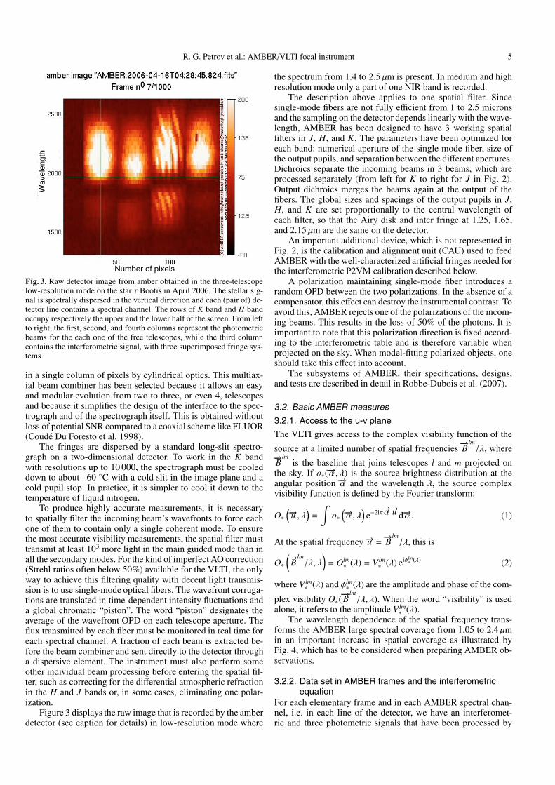
Fig. 3. Raw detector image from amber obtained in the three-telescopelow-resolution mode on the star τ Bootis in April 2006. The stellar sig-nal is spectrally dispersed in the vertical direction and each (pair of) de-tector line contains a spectral channel. The rows of K band and H bandoccupy respectively the upper and the lower half of the screen. From leftto right, the first, second, and fourth columns represent the photometricbeams for the each one of the free telescopes, while the third columncontains the interferometric signal, with three superimposed fringe sys-tems.

in a single column of pixels by cylindrical optics. This multiax-ial beam combiner has been selected because it allows an easyand modular evolution from two to three, or even 4, telescopesand because it simplifies the design of the interface to the spec-trograph and of the spectrograph itself. This is obtained withoutloss of potential SNR compared to a coaxial scheme like FLUOR(Coudé Du Foresto et al. 1998).

The fringes are dispersed by a standard long-slit spectro-graph on a two-dimensional detector. To work in the K bandwith resolutions up to 10 000, the spectrograph must be cooleddown to about –60 ◦C with a cold slit in the image plane and acold pupil stop. In practice, it is simpler to cool it down to thetemperature of liquid nitrogen.

To produce highly accurate measurements, it is necessaryto spatially filter the incoming beam’s wavefronts to force eachone of them to contain only a single coherent mode. To ensurethe most accurate visibility measurements, the spatial filter musttransmit at least 103 more light in the main guided mode than inall the secondary modes. For the kind of imperfect AO correction(Strehl ratios often below 50%) available for the VLTI, the onlyway to achieve this filtering quality with decent light transmis-sion is to use single-mode optical fibers. The wavefront corruga-tions are translated in time-dependent intensity fluctuations anda global chromatic “piston”. The word “piston” designates theaverage of the wavefront OPD on each telescope aperture. Theflux transmitted by each fiber must be monitored in real time foreach spectral channel. A fraction of each beam is extracted be-fore the beam combiner and sent directly to the detector througha dispersive element. The instrument must also perform someother individual beam processing before entering the spatial fil-ter, such as correcting for the differential atmospheric refractionin the H and J bands or, in some cases, eliminating one polar-ization.

Figure 3 displays the raw image that is recorded by the amberdetector (see caption for details) in low-resolution mode where

the spectrum from 1.4 to 2.5 µm is present. In medium and highresolution mode only a part of one NIR band is recorded.

The description above applies to one spatial filter. Sincesingle-mode fibers are not fully efficient from 1 to 2.5 micronsand the sampling on the detector depends linearly with the wave-length, AMBER has been designed to have 3 working spatialfilters in J, H, and K. The parameters have been optimized foreach band: numerical aperture of the single mode fiber, size ofthe output pupils, and separation between the different apertures.Dichroics separate the incoming beams in 3 beams, which areprocessed separately (from left for K to right for J in Fig. 2).Output dichroics merges the beams again at the output of thefibers. The global sizes and spacings of the output pupils in J,H, and K are set proportionally to the central wavelength ofeach filter, so that the Airy disk and inter fringe at 1.25, 1.65,and 2.15 µm are the same on the detector.

An important additional device, which is not represented inFig. 2, is the calibration and alignment unit (CAU) used to feedAMBER with the well-characterized artificial fringes needed forthe interferometric P2VM calibration described below.

A polarization maintaining single-mode fiber introduces arandom OPD between the two polarizations. In the absence of acompensator, this effect can destroy the instrumental contrast. Toavoid this, AMBER rejects one of the polarizations of the incom-ing beams. This results in the loss of 50% of the photons. It isimportant to note that this polarization direction is fixed accord-ing to the interferometric table and is therefore variable whenprojected on the sky. When model-fitting polarized objects, oneshould take this effect into account.

The subsystems of AMBER, their specifications, designs,and tests are described in detail in Robbe-Dubois et al. (2007).

3.2. Basic AMBER measures

3.2.1. Access to the u-v plane

The VLTI gives access to the complex visibility function of the

source at a limited number of spatial frequencies −→Blm/λ, where

−→B

lmis the baseline that joins telescopes l and m projected on

the sky. If o∗(−→α, λ) is the source brightness distribution at theangular position −→α and the wavelength λ, the source complexvisibility function is defined by the Fourier transform:

O∗(−→u , λ) = ∫

o∗(−→α, λ) e−2iπ−→α−→u d−→α. (1)

At the spatial frequency −→u = −→Blm/λ, this is

O∗(−→B

lm/λ, λ

)= Olm

∗ (λ) = Vlm∗ (λ) eiφlm∗ (λ) (2)

where Vlm∗ (λ) and φlm∗ (λ) are the amplitude and phase of the com-

plex visibility O∗(−→B

lm/λ, λ). When the word “visibility” is used

alone, it refers to the amplitude Vlm∗ (λ).The wavelength dependence of the spatial frequency trans-

forms the AMBER large spectral coverage from 1.05 to 2.4 µmin an important increase in spatial coverage as illustrated byFig. 4, which has to be considered when preparing AMBER ob-servations.

3.2.2. Data set in AMBER frames and the interferometricequation

For each elementary frame and in each AMBER spectral chan-nel, i.e. in each line of the detector, we have an interferomet-ric and three photometric signals that have been processed by

6 R. G. Petrov et al.: AMBER/VLTI focal instrument

Fig. 4. Exploration of the u-v plane using spec-tral coverage. The two figures represent the typ-ical fringed visibility function as a function ofu and v, as produced by a binary. On the left wehave the u-v tracks obtained with a single spec-tral channel and 10 hours of observations withUT1-UT3-UT4. On the right, we represent theu-v coverage obtained from 1.05 to 2.4 micronswith only one snapshot observation with thesame telescopes. As demonstrated by (Millouret al. 2007), the constraints on the binary angu-lar separation are similar for the left and right u-v coverages, but in the spectrally resolved casewe obtain the spectra of the components in ad-dition.

the same optics and the same dispersive elements (as shown inFigs. 2 and 3). For a single-mode instrument, the Fourier inter-ferogram (Fourier transform of the fringe pattern in the interfer-ometric channel) is

I(−→u , λ) = P

(−→u , λ) nT∑1

ni∗(λ)

+P

⎛⎜⎜⎜⎜⎜⎜⎝−→u −−→B

i j

λ, λ

⎞⎟⎟⎟⎟⎟⎟⎠∑i� j

√ni∗(λ)n j

∗(λ)Vi jm (λ)eiφi j

m(λ) (3)

where P(−→u , λ) is the single-telescope transfer function at the spa-tial frequency −→u and wavelength λ, Vi j

m (λ) and φi jm(λ) are the

measured visibility and phase and ni∗(λ) is the total contributionof beam i to the source flux collected in the interferometric chan-nel. In the following we note ni∗, Vi j

m and φi jm for ni∗(λ), Vi j

m (λ) andφ

i jm(λ) respectively, except when the wavelength dependence is

explicitly used.

3.2.3. Basic Fourier estimator

The first term in Eq. (3) is the low-frequency peak affected onlyby a fixed instrumental term P(−→u ) and scaled by the total num-ber of photons Σni∗ collected in all beams. The second term is thefringe peak, with a phase φi j

m and an amplitude equal to the mea-

sured coherence flux√

ni∗nj∗V

i jm at frequency −→Bi j

/λ. The num-ber of photons ni∗ detected in each frame are deduced from thephotometric channels. In an ideal interferogram where the fringepeaks are fully separated, the measured visibility is obtained by

dividing the Fourier interferogram at frequency−→u = −→Bi j/λ by itsvalue at frequency

−→0 and correcting by the known photometry:

Vi jm eiφi j

m =I(−→Bi j

/λ)I(0)

∑ni∗√

ni∗nj∗e−iφi j

P . (4)

The e−iφi jP corresponds to a correction of the effect of the differ-

ential piston between beams i and j. The measured visibility is

Vi jm (λ) = Vi j

∗ (λ)Ci jI (λ) (5)

where Ci jI (λ) contains internal AMBER instrumental terms

Ci jA (λ), which are removed by the calibration procedure below.

It is also affected by the “piston jitter”, i.e. the variation of the

piston during acquisition of the frame. If ∆pi j is this jitter, sup-posed to be smaller than the total piston excursion (because weuse short frame times), we can consider that fringes were drift-ing almost linearly during the frame and the contrast loss is thengiven by

Ci jI (λ) = Ci j

A (λ)sin(π∆pi j/λ)π∆pi j/λ

, (6)

which can be corrected if the piston jitter within one frame canbe deduced from the piston variations between two consecutiveframes.

3.2.4. Modal visibility of a single-mode instrument

A single-mode fiber collects light within an “antenna” lobe f (−→α )describing the relative contribution of a point on the sky at an an-gular distance −→α of the pointing direction. The source observedby AMBER is integrated and weighted by this “antenna lobe”The instantaneous antenna function depends on the geometry ofthe fiber, and does so for each aperture PSF partially correctedby adaptive optics. The exact measured visibility also dependson the degree of coherence between the antenna functions ofeach individual aperture. Single-mode interferometers give ac-cess only to the “modal” visibility defined by relatively complexrelations to be found in Mège et al. (2003). It is important to notethat:

– For sources smaller than the Airy disk of individual aper-tures, the modal visibility is equal to the source visibility;

– For extended sources, there is no simple way to separate thecontributions of the source and of the individual aperturePSF. What has been done so far (van Boekel et al. 2003) is toconsider the object as the sum of a small source, for whichthe above applies, and of a source substantially larger thanthe Airy disk, which produces a completely incoherent con-tribution. When this is wrong, one should use the modal visi-bility in the model-fitting procedure, which assumes a modelof the average adaptive-optics corrected PSF. Some simpli-fications can be found for particular objects, such as doublestars.

A full discussion of this topic is beyond the scope of this pa-per. To our last present knowledge, the problem has not yet beenresolved for a general source. We now say that AMBER (andother VLTI or KeckI single-mode instruments) perform wellwhen the source is smaller than the individual aperture Airydisks (which is a severe restriction for interferometers with smallbaseline/diameters ratios). In the following we do not distinguish

R. G. Petrov et al.: AMBER/VLTI focal instrument 7

between the modal and the true complex visibility so use Vi j∗ eiφi j

∗

for both.

3.2.5. The pixel to visibility approach

Fully separating the fringe peaks in a multi-axial beam com-biner implies a large separation between output pupils (i.e. manyfringes per Airy disk) and a window that is much larger than theAiry disk and would thus imply reading a very large number ofpixels, which is not acceptable when one is limited by detectorread-out noise. To overcome the problem of partially overlap-ping fringe peaks, a generalization of the ABCD algorithm usedin the PTI interferometer (Colavita 1999) has been developed toestablish a linear relation between the values measured in eachpixel and the complex coherence for each baseline (for detailssee Tatulli et al. 2007b). Fundamentally, the technique consistsin finding the modulus and phase for each baseline, which allowsthe calibrated fringe shapes (the carrying waves) to be fitted inthe data. This fit is linear and is based on the visibility-to-pixelmatrix, computed from a set of calibration measurements usingthe artificial coherent source unit (CAU) of the instrument. Thesemeasurements are the photometry and interferometry from eachbeam alone and the interferograms for each pair of beams at 0and close to λ/2 OPD. This matrix is then inverted to get thepixel to visibility matrix (P2VM) used to obtain the complex vis-ibility in each frame from the intensities measured in each pixel.This P2VM matrix takes all stable instrumental effects into ac-count, such as the detector gain table, the shape and the overlapof the output fiber beams, and the instrument’s chromatic OPD.

Analytical computations and numerical simulations showthat this P2VM approach can be implemented without any SNRcost (Tatulli & LeBouquin 2006), at least when the SNR perframe is larger than 1.

3.3. AMBER observables

During the observation, we record NEXP exposures of NDITframes, each exposed during the detector integration time, DIT.Typically a calibrated point is made of NEXP = 5 exposures ofNDIT = 1000 frames of DIT = 20 to 100 ms. For each baselinelm, and in each spectral channel, we obtain a measure of theintensity and of the visibility amplitude Vlm

m (λ) and phase φlmm (λ),

used to derive the various AMBER observables.

3.3.1. Spectrum of the source

Each one of the photometric beams yields a spectrum of thesource within the chosen spectral window. The raw AMBERspectrum must be calibrated in intensity and in wavelength,which in medium and high resolution modes requires acquiringa spectral calibrator with a known continuum shape and spec-tral features as illustrated by Fig. 5. The spectrum is a crucialelement of AMBER model fitting. Simultaneous observations ofhigh-resolution infrared spectra, for example with the ISAACinstrument, have often been found to be very useful (Meillandet al. 2007b; Malbet et al. 2007).

3.3.2. Absolute visibility per spectral channel

The absolute visibility in each spectral channel is the direct re-sult of the P2VM data processing. As discussed above, the mea-sured absolute visibility is affected by the piston jitter withinone frame. This jitter should be frozen by VLTI fringe trackingor measured when the flux per frame is high enough. Currentlythis correction is impossible because the vibrations in the Unit

Fig. 5. Data used for spectral calibration. Top: source spectrum (γ2Vel);Middle: the calibrator star flat spectrum (shifted by –0.5); Bottom: thereference Gemini spectrum (shifted by –1). Note the atmospheric water-vapor doublets at 2.01 and 2.06 µm used for calibration in K-bandmedium-resolution observations.

Telescope produce a piston variation that is almost always largerthan λ between consecutive frames. A partial correction of theeffect is obtained using a calibrator star:

Vs(λ) =Vms(λ)Vmc(λ)

Vc(λ), (7)

where Vs(λ) is the calibrated visibility of the target, Vms(λ) andVmc(λ) are the visibilities measured on the target and on the cal-ibrator, and Vc(λ) is the known visibility of the calibrator. Thiscorrection is poor (0.03 to 0.07 visibility accuracy), if we cannotapply a frame-by-frame piston jitter correction. Then, it is partic-ularly important to have a frame-selection criterion, independentof flux and tending to select an equivalent set of frames for thescience and the calibration source. Currently the best solutionis to select calibrators with magnitudes comparable to the sci-ence source and to select the same percentage of best contrastsin both cases. Even with an excellent jitter correction, using acalibrator will always be necessary for good accuracy measure-ments to compensate for slow instrumental variations modifyingthe value of all the second-order instrumental defects. For ex-ample, a small change in the position of the CAU beams willchange the contrast of the CAU source and therefore the cor-rected instrumental contrast.

The absolute visibility mainly depends on the equivalent sizeof the source in the direction of the baseline. A fit of absolute vis-ibility as a function of baseline length allows us to estimate theequivalent radial intensity profile, such as the limb darkening.This has been illustrated by AMBER observations of η Carinaethat permitted Weigelt et al. (2007) to obtain a remarkable fitof the central-wind limb-darkening by Hillier & Lanz (2001)model. A fit of visibility as a function of position angle of theprojected baseline yields the source anisotropy, which can be re-lated to flattened inclined disks (Malbet et al. 2007), sometimescombined with a very strong polar flow (Meilland et al. 2007b)or an optical wind enhanced in the polar direction of a fast ro-tator (Domiciano de Souza et al. 2005; Weigelt et al. 2007) ora combination of all these factors. Distinguishing between thesepossibilities requires prior knowledge of the source. Visibilityalone does not allow axisymmetric and non axisymmetric solu-tions to be disentangled between (except with a very good u-vcoverage) and will be of little use if the structure of the objet iscompletely unknown.

8 R. G. Petrov et al.: AMBER/VLTI focal instrument

3.3.3. Differential visibility

The differential (or relative) visibility Vds(λ) is the source visi-bility in the spectral channel λ, often called work channel, cali-brated by the average visibility of a reference channel:

Vds(λ) =Vms(λ)Vref (λ)

(8)

where

Vref (λ j) =1

nλ − 2

⎛⎜⎜⎜⎜⎜⎝ nλ∑i=1

Vms(λi) − Vms(λ j)

⎞⎟⎟⎟⎟⎟⎠ . (9)

This is the standard way to build the reference channel inAMBER data processing. The users can choose many other def-initions of the reference channel, such as using selected contin-uum channels. The ideal is, of course, to use channels where thesource is known or particularly well-constrained, but in any case,the exact definition of the reference channel, which depends ofthe source and of data processing constraints, must be injectedin the model fitting. The important feature is that the differen-tial visibility is independent of most of the systematic effectsaffecting the absolute visibility, and it does not need the use ofa calibrator star. In particular, the differential visibility will beinsensitive to the piston jitter over a limited wavelength range.

The relative visibility basically yields the same physical in-formation as the spectrally-resolved absolute visibility, but it ismuch better calibrated, at the cost of losing information on thereference channel.

3.3.4. Differential phase

In optical, as well as in radio astronomy, source phase informa-tion refers to the phase of its complex visibility. In a single-modeinterferogram, the phase is related to the position of the fringes,and in the absence of nanometer accuracy metrology, the mea-sured phase φms(λ) is affected by an unknown instrumental termlinked to the VLTI+AMBER differential piston δlm and to theinstantaneous atmospheric piston plm between beams l and m:

φms(λ) = φs(λ) + 2π(δ + p)/λ. (10)

Introducing a development of the source phase φs(λ), as a func-tion of the wave number σ = 1/λ:

φs(λ) = a0 + a1σ + ϕsh(λ) = ϕsl(λ) + ϕsl(λ) (11)

where ϕsl(λ) stands for the straight line that can be fitted throughthe measured phase and that contains the piston residual, as wellas the equivalent piston of the source phase averaged over thereference channel. The higher terms of the phase polynomial de-velopment ϕsl(λ) are the source information, which can be ex-tracted from differential phase measurements. We first fit themeasured phase φms(λ) phase with a linear function of σ. Thenwe correct the coherent flux C(λ) for this linear phase phasor,and we integrate it in a reference channel:

Cref (λ j) =nλ∑i=1

C(λi)e−iϕsl(λi) −C(λ j)e

−iϕsl(λ j). (12)

The differential phase is defined by:

ϕds(λ) = arg(〈(C(λ)C∗ref(λ)〉). (13)

If the reference channel has been defined in channels where thesource phase is equal to 0, for example in the spectral continuumchannel of a point-like or a symmetrical source,

Cref (λ) = ΣλcontC(λ)e−iϕsl(λ) = Vrefe−2iπ(δ+p)/λ. (14)

This yields the higher-order term ϕsl(λ). We obtain phase infor-mation on the source, but we have lost the equivalent piston ofthe reference channel.

As for the differential visibility, there are many ways to de-fine the reference channel, which must be injected in the sourcemodel-fitting process. Equation (14) gives the definition of thereference channel used in AMBER data processing.

A remarkable feature of the differential phase is that, fornon resolved (i.e. smaller than λ/B) sources, it is proportionalto the variation of the photocenter of the source (Petrov 1989).Given a sufficient SNR, the photocenter variation with λ can bemeasured on very unresolved sources with many very rich as-trophysical applications. This includes unresolved circumstellardisks and imaging of unresolved spotted stars (Petrov 1988) orof non radial oscillation modes (Jankov et al. 2002). One of themost promising applications is the resolution and the kinematicsof QSO BLR. With a fringe tracking up to K � 12, one shouldbe able to measure photocenter variations and therefore directdistances for some Cepheids of the Magellan Cloud.

3.3.5. Closure phase

The closure phase between baselines −−→B12, −−→B23 and −−→B31 is thephase of the average “bispectral product” of the coherent fluxes

ψ123 = arg(〈C12C23C∗31〉), (15)

and it is a very classical property of long-baseline interferometrythat this closure phase is independent of any OPD terms affectingindividually each beam. This includes the achromatic piston, aswell as the chromatic OPD:

ψ123 = φ∗12 + φ∗23 − φ∗13 + φd12 + φd23 − φd13 (16)

where φdi j are error terms linked to the baseline i j, due for ex-ample to a change in the detector gain table since the calibra-tion of the P2VM. Usually, these terms are very small so it canbe considered that for many applications the closure phase isonly a function of the source. Unlike the differential phase, theclosure phase is independent of any assumption on a referencechannel. A sufficient number of closure phases, combined withaccurate visibility measurements, allows reconstruction of rel-atively complex images, as demonstrated by the 2006 “imagereconstruction beauty contest” (Lawson et al. 2006), which wasbased on “realistic”, low-contrast, AMBER 3AT data, obtainedover three simulated nights of observations. The best three imagereconstructions were quite good, demonstrating a real imagingcapability with a three-telescope optical interferometer.

For any triplet of baselines, the closure phase is zero for anyaxisymmetric object. For non-axisymmetric candidates, the clo-sure phase decreases with the third power of the object angu-lar size when it is getting unresolved. Then, a non zero closurephase is a strong indication of a source with an interferomet-rically resolved non-axisymmetric feature, like the binary sys-tem γ2 Velorum (Millour et al. 2007) or the η Carinae wind inthe blue part of the Brγ line (Weigelt et al. 2007).

R. G. Petrov et al.: AMBER/VLTI focal instrument 9

4. AMBER current and potential performances

In this section we first present the expected performances ofAMBER on the VLTI and then briefly discuss their current statuswith some indications of the cause and the predictable evolutionof limitations.

4.1. Fundamental error on the visibility

The AMBER measures are affected first by the photon noise ofthe source and of the background and by the detector read-outnoise, called the fundamental noises. In the following we givethe errors on the visibility and the phases using the standardFourier formalism (among many others, see for example Petrovet al. 1986), which has been shown to be sufficient for SNR es-timations during AMBER commissioning, when we comparedFourier SNR estimation and statistics on the measures and foundthem in good agreement well within a factor

√2. From the in-

terferometric Eq. (3) and the complex visibility estimator 4 it ispossible to derive the error on the visibility estimator (with theapproximation that all noises and pixels are statistically indepen-dent):

σVi j =1√nin j

⎡⎢⎢⎢⎢⎢⎣√∑

i

n∗i +∑

i

nBi + npσ2R

+Vi j

m

2

(σ∗i

2√

n∗i+

σ∗ j

2√

n∗ j

) ⎤⎥⎥⎥⎥⎥⎦ (17)

where n∗i and nBi are the number of source and background pho-tons per frame in one spectral channel, np is the number of pix-els used to record one spectral channel, and σR is the detectorread out noise per pixel. The first term of this equation resultsfrom the contribution of fundamental noises to the error on thecoherent flux and the second term results from the photometriccorrection applied to obtain the visibility from the coherent flux(Tatulli et al. 2007b). The value of σ∗i is the relative error on themeasure of the contribution of beam i to the flux in the interfer-ometric channel:

σ∗i =

√n∗i + nBi + npσ

2R

n∗i· (18)

In AMBER, the contribution of the thermal background issmaller than the read-out noise for all the usual short exposuretimes (≤100 ms) except after 2.3 µm. Then two cases must beconsidered. At high flux, when n∗i > npσ

2R, the relative error on

the visibility is given by

Vi jm

σVi j

=Vi j

m√

Mn∗√nT

(19)

where M is the number of frames and n∗ is the average numberof photons per channel, per frame, and per telescope, which aresupposed equal for all telescopes. The performance of AMBER,defined here as, for example, the time needed to achieve a givenSNR, is proportional to n∗V2. Then, the coherent magnitude isgiven by the flux n∗V2. This applies for relatively bright and low-contrast sources. At lower flux, when n∗i < npσ

2R,

Vi jm

σVi j

=n∗V

i jm√

npσ2R(1 + Vi j

m/2√

n∗)� n∗V

i jm√

npσ2R

· (20)

The performance of AMBER is proportional to (n∗V)2 and thecoherent magnitude is given by the flux n∗V . This case representsfaint sources with whatever contrasts.

Table 2. Number of photons per frame and per channel needed forthe frame to contribute to the ensemble averages, as a function ofthe observing mode and considering the measured and the potential(vibration-free) atmosphere+VLTI+AMBER visibility.

Mode actual Visibility potential VisibilityLow Vactual = 0.12 Vpotential = 0.5Resolution 581 phots 187 photsMedium Vactual = 0.14 Vpotential = 0.6Resolution 507 phots 166 phots

Table 3. Number of photons collected per 50 ms frame and per spectralchannel in the K band in different observation modes.

Observation best 20% averageMedium Resolution 1000 530K = 4.9Low Resolution 4250 2540K = 8.2

Table 4. Current, potential, and achieved limiting magnitudes ofAMBER in the K band, for 50 ms frames.

Mode MR MR LR LRConditions best 20% average best 20% averageCurrent 5.6 4.9 10.2 9.7Potential 6.8 6.1 11.5 10.9Achieved – 4.9 – 8.6

4.2. Limiting magnitude

The limiting magnitude of AMBER is set by Vi jmσV� 1 for

the average spectral channel. The actual data processing showsthat frames not complying with this criteria yield absurd es-timated complex visibility that destroy ensemble averages. Inpractice, such frames are eliminated in the data processing.During the first commissioning of AMBER, frame times be-tween 50 ms and 100 ms gave contrasts between 0.15 < V < 0.2on an unresolved calibrator. Knowing that the average measuredAMBER instrumental contrast is V = 0.8 in medium resolu-tion (MR) and V = 0.7 in low resolution (LR), this yields anactual VLTI+atmosphere contrast of Vactual = 0.12 in low res-olution and Vactual = 0.14 in medium resolution. If the VLTIwas only limited by the atmospheric piston jitter and by vi-brations “within the specifications” (i.e. 10% of contrast lossdue to VLTI non atmospheric effects), these contrasts would beVpotential = 0.6 in medium resolution and Vpotential = 0.7 in lowresolution. The commissioning with AT indeed confirmed theseVLTI+atmosphere contrast values. Putting these actual and po-tential contrast values in Eq. (20) yields the number of pho-tons per channel and per frame needed to achieve the condi-

tion Vi jmσV� 1. These values are given in Table 2. Table 3 gives

the number of photons per frame and per spectral channel col-lected during the first commissioning of the instrument, beforethe implementation of the IRIS focal laboratory “infrared imagesensor”. Combining the collected flux given in Table 3 and theminimum needed flux in Table 2 yields the current and poten-tial limiting magnitudes of AMBER displayed in Table 4. The“current” value corresponds to the currently measured fluxesand atmosphere+VLTI+AMBER instrumental visibility. The“achieved” value gives the magnitude of calibrators on which ac-tual fringes have been recorded. This value is available only foraverage conditions because of the limited number of attempts. InLR mode there is a gap between the “current” and the “achieved”values. The most likely explanation was the fast fringe drift dueto the poor quality of early delay-line models. It is worth

10 R. G. Petrov et al.: AMBER/VLTI focal instrument

noting that the current values should allow a successful obser-vation of NGC1068 and maybe of a couple of other AGN (ifthe MACAO adaptive optics behave correctly on these faint andextended sources in the visible).

The “potential” value corresponds to the currently measuredtransmissions combined with a VLTI+atmosphere contrast withreduced vibrations allowing the UT to approach the AT vibrationlevels and the initial VLTI specifications. The limiting magni-tude in LR should then be K ≥ 11, therefore compliant withAMBER specifications for an ambitious AGN program. Thislimit should be extended to all modes as soon as fringe track-ing is operational. The final limit will be set by the quality ofthe vibration correction. These limiting magnitudes correspondto an SNR = 1 per spectral channel and per frame. Achievingan accuracy on V � 0.01 requires averaging 104 50 ms frames,which requires between 500 and 1500 seconds of actual obser-vations.

4.3. Accuracy on the differential phase

By analogy with the visibility error computation, the phase un-certainty is written as

σφ � σV/√

2

Vi jm

· (21)

Usually the reference channel is set much larger than the indi-vidual spectral channel, and it contributes little to the error onthe differential phase, which allows the above estimation to beused for the differential phase. Typically a visibility fundamentalSNR of 100 therefore corresponds to a differential phase error of0.007 radians. However, the differential phase is not affected bythe same calibration problems. Currently we approach 10−3 radon very bright sources for which we should have smaller errors.We are currently limited by data-processing problems (problemof the optimum correction of the frame-by-frame piston) and bythe difficulty of fitting variable chromatic OPD, mainly due tovariations in the thickness of water vapor in the tunnels.

4.4. Accuracy on the closure phase

In theory, the accuracy on the closure phase should be about√3σφ. However, with the UT, the number of frames where the

three baselines simultaneously show good fringes is extremelysmall. In practice, the limit is about 0.01 rad, even for very brightsources. The situation is supposed to be very different with threeAT. The current impossibility of having very accurate closurephases with 3 UT is a serious drawback for the ESP program.

5. Operating AMBERAMBER is working within the standard Science Operationsframework in use for the VLT instruments. The VLTI ScienceOperations is described in Rantakyrö et al. (2004), so here wehighlight only those issues relevant to the AMBER general user,who can concentrate on the scientific objectives of the run ratherthan on details of the telescopes, VLTI, and AMBER operations.In this framework, the user’s main, if not single, concern is tomake certain that the proper calibration procedures are used.

5.1. Internal P2VM calibration

The first calibration is to measure the P2VM specific to the ob-serving mode. The P2VM can be modified by any change inthe spectrograph setup, and the operating procedure will forcethe observer to measure a new P2VM for any new set up,prior to science observations. The observer must choose between

a standard-accuracy P2VM, to be within the specifications ofAMBER, and a high-accuracy one, to try to approach the goalsof highest accuracy.

– Standard-accuracy P2VM: to achieve 0.01 absolute visibil-ity accuracy, a P2VM is computed with about 105 photonsrecorded in each line of each interferogram. With the maxi-mum flux allowed without saturating the detector, a full cal-ibration takes about 7 min, i.e. about the time for the VLTIto acquire the source and put it through all its subsystems.The errors introduced by the standard P2VM are substan-tially decreased for differential phase (0.001 radians) or vis-ibility (0.001);

– High-accuracy P2VM: In practice, extremely high accuracy(10−4 rad) is expected only with differential measures anda 107-photon P2VM should be sufficient. This needs threehours before the beginning or after the end of the night, soit implies restrictions on the scheduling of setup changes. Itstill has to be investigated whether the stability of the P2VMover a few hours is good enough to allow the use of such along calibration.

5.2. Detector noise and background calibrationAny set of observations includes observing dark images (warmshutters closed) and sky images (telescopes offset) that are laterused in the data reduction. The observer chooses the number ofdark and sky exposures. The standard value is currently one darkand one sky for five source exposures. The observers also definethe offset of the telescopes, to make sure that the “sky” directionis actually source free.

5.3. External calibration using a calibratorAll interferometric observables, including the differential andthe closure phases, are affected by systematic effects that canbe removed or reduced using a calibrator star with known com-plex visibility. An important task for the observer is to choosegood calibrators. Ideally a calibrator is a point source; however,finding strictly non resolved and bright-enough stars is a realproblem. A good calibrator is then a single, non variable star,which can be considered as a uniform disk with a known diame-ter. Then the visibility of the calibrator is known and its differen-tial and closure phases are zero. “Primary” calibrators, found indatabases of measured diameters for bright stars (Richichi et al.2004), are used when they are close enough to the science tar-get in magnitude, visibility and angular coordinates. The samedatabases of measured diameters have been used to validate toolsfor selecting and qualifying much more numerous “secondary”calibrators from the color indices found in astronomical cata-logues (Bonneau et al. 2006).

5.4. Spectral calibrationA spectral calibrator is required for medium and high spectral-resolution modes. Usually, it is a star with a clean and well-known continuum allowing calibration of the relative intensitiesrecorded by AMBER and use of the telluric lines for accuratewavelength-table calibration. It is also strongly advised to sys-tematically obtain a calibrated high-resolution spectrum of thesource during or close to the interferometric run, from ISAAC(Moorwood et al. 1999) or other spectrographs.

5.5. Beam commutation for closure and differential phasecalibration

To have accurate differential and closure phases, the observercan use the “differential” observing mode, in which a beam

R. G. Petrov et al.: AMBER/VLTI focal instrument 11

commutation device (BCD) is used to exchange beams 1 and 2at the entrance of AMBER at the end of each exposure. This in-verts the source differential phase for B12 and the source closurephase without changing the instrumental terms. Then, comput-ing the differences between exposures with and without beamcommutation (BCD “in” and “out”) yields differential and clo-sure phase with strongly reduced instrumental effects (Petrovet al. 2003; Vannier et al. 2006). The commutation takes lessthan 5 s and can therefore be performed much more often than ascience-calibrator exchange.

5.6. Observing

Observing is performed through the VLT control system usingthe standard tool (P2PP: Phase 2 Preparation Package) to createblocks of observations. These blocks contain several procedures,called templates, to set up the instrument, to point the interfer-ometer, to optimize the beam injection into AMBER, to searchfor fringes, and to acquire observation data. P2PP allows chang-ing some of the parameters for these procedures, like the wave-length range, the spectral dispersion, or the detector integrationtime.

The observation block is executed through the breaker of ob-serving blocks (BOB), which ensures that all steps are carriedout successfully. Some of the templates are executed in parallel,such as the injection of light into the AMBER fibers for eachtelescope. The night astronomer has control over BOB and canabort or redo part of the procedures. The system also asks thenight astronomer to make critical choices such as whether tocontinue or abort a so far unsuccessful fringe search.

5.7. Quick look, online data reduction, archiving

As for other VLT instruments, AMBER has a standard real-timedisplay that shows the raw data. It also has a quick-look monitorthat displays visibilities and phases reduced online in almost realtime. The data is automatically archived and passed to the datareduction pipeline that analyses the data almost immediately af-ter acquisition so that the night astronomer and/or the visitingastronomer can check the quality of the data.

6. ConclusionWith its coherent combination of three unit telescopes, AMBERcurrently makes the VLTI the world’s largest optical telescopewith a total surface >150 m2 and a maximum baseline >130 mcorresponding to a spatial resolution than 3 mas in the K band.

The capacity to measure closure phases gives AMBER animage-reconstruction capability with different configurations ofthree VLTI telescopes. The measurement of individual closurephases already yields decisive constraints on the source geome-try. AMBER includes a high-performance infrared-cooled spec-trograph allowing the structure and the physics of the sourceto be constrained by comparing the measures at different wave-lengths. Differential interferometry based on simultaneous inter-ferometric measures in different spectral channels yields a gainin accuracy of at least a factor 10. Analyzing spectral channelssimultaneously boosts the uniqueness and robustness of mea-sured parameters and images, particularly with spectral regular-ization functions. At low spectral resolution, the spectral cov-erage massively increases the instantaneous spatial coverage.AMBER made its first fringes in Paranal in the second quar-ter of 2004. For the general user, the first 3-UT period startedin October 2005 and 3-AT open time is starting in April 2007.Currently it is possible to observe in low, medium, and high res-olution in the H and K bands. The full potential in the medium

and high spectral resolution depends on the availability of thethree-telescope fringe tracker FINITO, which has already beensuccessfully tested with AT and will very likely be available withATs in October 2007. With the UTs, this depends on the qualityof the correction of the vibrations that currently affect the UTCoudé trains.

The first astrophysical observations in 2004 and 2005 hasled to a set of refereed papers that can be found in this vol-ume. They all illustrate the power of the spectral dimension ofinterferometric measures in situations of very poor u-v coverage.On young Herbig stars with high mass (MWC 297; Malbet et al.2007) and intermediate mass (HD 104237; Tatulli et al. 2007a),the variation of visibility through Brγ allowed them to discussthe connection between dust envelope and wind-driven gas andtheir relative geometry. On the Be star α Arae (Meilland et al.2007b), observations in the continuum and in the Brγ line al-lowed severe constraints on a wind found to be axisymmetricwith a thin equatorial disk in Keplerian rotation and a very strongpolar flow. Another Be star, κ CMa (Meilland et al. 2007a),showed a very different, small, non axisymmetric, and proba-bly non-Keplerian envelope. The dusty B[e] star CPD-57◦2874(Domiciano de Souza et al. 2007), observed with AMBER andMIDI, has non-spherical dust and gas envelopes with differentglobal geometries, perhaps again due to polar gas outflows. Forthe Wolf Rayet + O binary system γ2 Velorum (Millour et al.2007), measures including a strong closure phase in the contin-uum and in various carbon and helium emission lines, allowedthe separation of the components spectra, the measure of the an-gular separation implying a revision of the Hipparcos distance,and the detection of material outside the immediate vicinity ofthe components that might be the signature of the wind-windcollision. Measurements in medium and high spectral resolu-tion of the most luminous and massive luminous blue variableη Carinae (Weigelt et al. 2007), allowed reconstruction of a cen-tral, optically-thick, wind structure elongated in the direction ofthe axis of the Homonculus nebulae and well-modeled in thecontinuum and emission lines with remarkable agreement withthe radiative transfer code of Hillier & Lanz (2001). Last butnot least, Chesneau et al. (2007) reported the early AMBER in-terferometric observation of the outburst of RS Oph performed5.5 days after the outburst which provided an estimation of theextent of the continuum, Brγ and He I 2.06 µm forming re-gions and some physical constraints on the ejection process. Theglobal picture that emerges is a non-spherical fireball at high-velocity expansion.

The transmission measured on AMBER and the VLTI showsthat the current coherent limiting magnitude is K � 9.0 with aVLTI+atmosphere fringe contrast of 0.12. When the correctionof the UT vibration allow a VLTI+atmosphere fringe contrast of0.5, the limiting coherent magnitude of AMBER on the VLTIwill reach K � 11.5 in the 20% best-seeing conditions. Thiswill allow breakthrough science on a large number of AGN andQSO. With the ATs, the VLTI+atmosphere fringe contrast al-ready ranges from 0.5 to 0.9. When FINITO is operational, allspectral resolution modes will be accessible on the AT for K � 6in average conditions and K ≥ 7 in the 20% best conditions, withenormous possibilities in stellar physics.

Acknowledgements. The AMBER project4 was founded by the French CentreNational de la Recherche Scientifique (CNRS), the Max Planck Institutefür Radioastronomie (MPIfR) in Bonn, the Osservatorio Astrofisico diArcetri (OAA) in Firenze, the French Region Provence Alpes Côte D’Azur,

4 The structure and members of the AMBER Consortium can befound in the website: http://amber.obs.ujf-grenoble.fr

12 R. G. Petrov et al.: AMBER/VLTI focal instrument

and the European Southern Observatory (ESO). The CNRS funding has beenmade through the Institut National des Sciences de l’Univers (INSU) and itsProgrammes Nationaux (ASHRA, PNPS, PNP).The OAA co-authors acknowledge partial support from MIUR grants to theArcetri Observatory (A LBT interferometric arm, and analysis of VLTI in-terferometric data and From Stars to Planets: accretion, disk evolution andplanet formation) and from INAF grants to the Arcetri Observatory (Stellar andExtragalactic Astrophysics with Optical Interferometry). C. Gil’s work was sup-ported in part by the Fundação para a Ciência e a Tecnologia through projectPOCTI/CTE-AST/55691/2004 from POCTI, with funds from the European pro-gram FEDER.The preparation and interpretation of AMBER observations benefit from thetools developed by the Jean-Marie Mariotti Center for optical interferometryJMMC5 and from the databases of the Centre de Données Stellaires (CDS), andof the Smithsonian/NASA Astrophysics Data System (ADS).We would like to thank the successive directors of INSU/CNRS, G. Debouzy,F. Casoli, and A.-M. Lagrange, along with the ASHRA president P. Léna andthe VLT program manager M. Tarenghi of ESO for their crucial help in set-ting up and supporting the Consortium. We also thank S. Bensammar, V. Coudédu Foresto, and G. Perrin for their advice in defining the AMBER concept andConsortium.We are very grateful to the ESO staff in Garching and Paranal for their help inthe design and commissioning of AMBER.The key mechanical design and manufacturing have been provided by theDivision Technique de l’INSU and by the mechanical workshops of theObservatoire de Bordeaux, Observatoire de la Côte d’Azur, and Université deNice.

ReferencesAkeson, R. L., Swain, M. R., & Colavita, M. M. 2000, in Interferometry in

Optical Astronomy, ed. P. J. Léna & A. Quirrenbach, Proc. SPIE, 4006, 321Antonucci, R. R. J. & Miller, J. S. 1985, ApJ, 297, 621Barman, T. S., Hauschildt, P. H., & Allard, F. 2001, ApJ, 556, 885Bonneau, D., Clausse, J.-M., Delfosse, X., et al. 2006, A&A, 456, 789Chesneau, O., Nardetto, N., Millour, F., et al. 2007, A&A, 464, 119Colavita, M. M. 1999, PASP, 111, 111Colavita, M., Akeson, R., Wizinowich, P., et al. 2003, ApJ, 592, L83Colavita, M. M., Wallace, J. K., Hines, B. E., et al. 1999, ApJ, 510, 505Coudé Du Foresto, V., Perrin, G., Ruilier, C., et al. 1998, in Astronomical

Interferometry, ed. R. D. Reasenberg, Proc. SPIE V, 3350, 856Coudé du Foresto, V., Bordé, P. J., Mérand, A., et al. 2003, in Interferometry for

Optical Astronomy II, ed. W. A. Traub, Proc. SPIE, 4838, 280Delplancke, F., Nijenhuis, J., de Man, H., et al. 2004, in New Frontiers in Stellar

Interferometry, ed. W. A. Traub, Proc. SPIE, 5491, 1528Domiciano de Souza, A., Kervella, P., Jankov, S., et al. 2005, A&A, 442, 567Domiciano de Souza, A., Driebe, T., Chesneau, O., et al. 2007, A&A, 464, 81Gai, M., Menardi, S., Cesare, S., et al. 2004, in New Frontiers in Stellar

Interferometry, ed. W. A. Traub, Proc. SPIE 5491, 528Glindemann, A., Albertsen, M., Andolfato, L., et al. 2004, in New Frontiers in

Stellar Interferometry, ed. W. A. Traub, Proc. SPIE, 5491, 447Glindemann, A., Ballester, P., Bauvir, B., et al. 2001a, The Messenger, 106, 1Glindemann, A., Bauvir, B., Delplancke, F., et al. 2001b, The Messenger, 104, 2Hillier, D. J. & Lanz, T. 2001, in Spectroscopic Challenges of Photoionized

Plasmas, ed. G. Ferland & D. W. Savin, ASP Conf. Ser., 247, 343Jaffe, W., Meisenheimer, K., Röttgering, H. J. A., et al. 2004, Nature, 429, 47Jankov, S., Vakili, F., Domiciano de Souza, Jr., A., & Janot-Pacheco, E. 2002, in

IAU Coll. 185: Radial and Nonradial Pulsationsn as Probes of Stellar Physics,ed. C. Aerts, T. R. Bedding, & J. Christensen-Dalsgaard, ASP Conf. Ser., 259,172

Kervella, P., Gitton, P. B., Ségransan, D., et al. 2003, in Interferometry forOptical Astronomy II, ed. W. A. Traub, Proc SPIE, 4838, 858

Lawson, P. R., Cotton, W. D., Hummel, C. A., et al. 2006, in Advances in StellarInterferometry, ed. J. Monnier, M. Schöller, & W. C. Danchi, Proc. SPIE,6268

Leinert, C. 2004, in New Frontiers in Stellar Interferometry, ed. W. A. Traub,Proc SPIE, 5491, 19

Leinert, C., Graser, U., Przygodda, F., et al. 2003, Ap&SS, 286, 73Malbet, F. 2003, Ap&SS, 286, 131Malbet, F., Benisty, M., De Wit, W. J., et al. 2007, A&A, 464, 43Marconi, A., Maiolino, R., & Petrov, R. G. 2003, Ap&SS, 286, 245Mège, P., Malbet, F., & Chelli, A. 2003, in Interferometry for Optical Astronomy

II, ed. W. A. Traub, 329, Proc. SPIE, 4838,Meilland, A., Millour, F., Stee, P., et al. 2007a, A&A, 464, 73

5 The JMMC is a center providing software tools for optical interfer-ometry described on the website: http://www.jmmc.fr

Meilland, A., Stee, P., Vannier, M., et al. 2007b, A&A, 464, 59Millan-Gabet, R., Malbet, F., Akeson, R., et al. 2007, Protostars and Planets V,

539Millour, S., Petrov, R., Chesneau, O., et al. 2007, A&A, 464, 107Moorwood, A., Cuby, J.-G., Ballester, P., et al. 1999, The Messenger, 95, 1Mourard, D., Abe, L., Domiciano, A., et al. 2003, in Interferometry for Optical

Astronomy II, ed. W. A. Traub, Proc. SPIE, 4838, 9Paresce, F., Delplancke, F., Derie, F., et al. 2003a, in Interferometry for Optical

Astronomy II, ed. W. A. Traub, Proc. SPIE, 4838, 486Paresce, F., Mourard, D., Bedding, T., et al. 1996, The Messenger, 83, 14Paresce, F., Van Boekel, R., Correia, S., et al. 2003b, in Interferometry for

Optical Astronomy II, ed. W. A. Traub, Proc SPIE, 4838, 235Petrov, R., Roddier, F., & Aime, C. 1986, Opt. Soc. Am. J. A: Optics and Image

Science 3, 634Petrov, R. G. 1988, in NOAO-ESO Conference on High-Resolution Imaging

by Interferometry: Ground-Based Interferometry at Visible and InfraredWavelengths, ed. F. Merkle, 235

Petrov, R. G. 1989, in Diffraction-Limited Imaging with Very Large Telescopes,ed. D. M. Alloin & J.-M. Mariotti, NATO ASIC Proc., 274, 249

Petrov, R. G., Vannier, M., Lopez, B., et al. 2003, in EAS Publ. Series, ed.C. Aime & R. Soummer, 297

Rantakyrö, F. T., Galliano, E., Hummel, C. A., et al. 2004, in New Frontiers inStellar Interferometry, ed. W. A. Traub, Proc. SPIE, 5491, 1690

Richichi, A., Percheron, I., & Khristoforova, M. 2004, VizieR Online DataCatalog, 343, 10773

Robbe-Dubois, S., Lagarde, S., Antonelli, P., et al. 2007, A&A, 464, 13Ségransan, D., Beuzit, J.-L., Delfosse, X., et al. 2000, in Interferometry in

Optical Astronomy, ed. P. J. Léna & A. Quirrenbach, Proc. SPIE, 4006, 269Swain, M., Vasisht, G., Akeson, R., et al. 2003, ApJ, 596, L163Tatulli, E. & LeBouquin, J.-B. 2006, MNRAS, 368, 1159Tatulli, E., Isella, A., Natta, A., et al. 2007a, A&A, 464, 55Tatulli, E., Millour, F., Chelli, A., et al. 2007b, A&A, 464, 29van Boekel, R., Kervella, P., Schöller, M., et al. 2003, A&A, 410, L37Vannier, M., Petrov, R. G., Lopez, B., & Millour, F. 2006, MNRAS, 367, 825Weigelt, G., Kraus, S., Driebe, T., et al. 2007, A&A, 464, 87Wittkowski, M., Kervella, P., Arsenault, R., et al. 2004, A&A, 418, L39

1 Laboratoire Universitaire d’Astrophysique de Nice, UMR 6525Université de Nice, Sophia Antipolis/CNRS, Parc Valrose, 06108Nice Cedex 2, France, e-mail: Romain.Petrov@unice.fr

2 Laboratoire d’Astrophysique de Grenoble, UMR 5571 UniversitéJoseph Fourier/CNRS, BP 53, 38041 Grenoble Cedex 9, Francee-mail: Fabien.Malbet@obs.ujf-grenoble.fr

3 Max-Planck-Institut für Radioastronomie, Auf dem Hügel 69,53121 Bonn, Germany

4 Laboratoire Gemini, UMR 6203 Observatoire de la Côted’Azur/CNRS, BP 4229, 06304 Nice Cedex 4, France

5 INAF-Osservatorio Astrofisico di Arcetri, Istituto Nazionale diAstrofisica, Largo E. Fermi 5, 50125 Firenze, Italy

6 European Southern Observatory, Casilla 19001, Santiago 19, Chile7 ONERA/DOTA, 29 av de la Division Leclerc, BP 72, 92322

Chatillon Cedex, France8 Centre de Recherche Astronomique de Lyon, UMR 5574 Université

Claude Bernard/CNRS, 9 avenue Charles André, 69561 Saint GenisLaval Cedex, France

9 Division Technique INSU/CNRS UPS 855, 1 place Aristide Briand,92195 Meudon Cedex, France

10 IRCOM, UMR 6615 Université de Limoges/CNRS, 123 avenueAlbert Thomas, 87060 Limoges Cedex, France

11 European Southern Observatory, Karl Schwarzschild Strasse 2,85748 Garching, Germany

12 Kiepenheuer Institut für Sonnenphysik, Schöneckstr. 6, 79104Freiburg, Germany

13 Instituut voor Sterrenkunde, KU-Leuven, Celestijnenlaan 200D,3001 Leuven, Belgium

14 Centro de Astrofísica da Universidade do Porto, Rua das Estrelas -4150-762 Porto, Portugal

15 Laboratoire Astrophysique de Toulouse, UMR 5572 Université PaulSabatier/CNRS, BP 826, 65008 Tarbes Cedex, France

16 Departamento de Astronomia, Universidad de Chile, Chile