A Deployable Telescope for Sub-Meter Resolutions from ...

iii

A Deployable Telescope for Sub-Meter Resolutions

from MicroSatellite Platforms

Dennis Dolkens

(1305921)

Master Thesis

Department of Space Engineering

Faculty of Aerospace Engineering

Delft University of Technology

February 2015

iv

A Deployable Telescope for Sub-Meter Resolutions from NanoSatellite Platforms

Master Thesis, Copyright © 2015 by Dennis Dolkens

Front cover: Background image courtesy of NASA

GRADUATION COMMITTEE:

prof. dr. E.K.A. Gill – Space Systems Engineering, TU Delft

dr. J.M. Kuiper – Space Systems Engineering, TU Delft

dr. D.M. Stam – Astrodynamics & Space Systems, TU Delft

ir. B.T.G de Goeij – TNO

v

“Optical experience, developing in us through study, teaches us to see”

― Paul Cézanne (1905)

vii

Abstract

Sub-meter resolution satellite imagery serves a more and more important role in applications ranging from

environmental protection, disaster response and precision farming to defence and security. Earth

Observation at these resolutions has long been the realm of large and heavy telescopes. The costs of

building and launching such systems are enormous, which results in high image costs, limited availability

and long revisit times. Using synthetic aperture technology, instruments can now be developed that can

reach these resolutions using a substantially smaller launch volume and mass.

In this thesis, a conceptual design is presented of a deployable synthetic aperture instrument. The

instrument can reach a ground resolution of 25 cm from an orbital altitude of 500 km, which is compliant

with current state-of-the-art systems, such GeoEye-2 and Worldview-3. The thesis covers the optical and

mechanical design of the instrument, as well as the calibration strategy and image processing techniques

that are required to ensure a good end-to-end image quality.

An optical concept study was performed in which two types of synthetic aperture instruments were

compared: the Fizeau synthetic aperture, a telescope with a segmented primary mirror, and the

Michelson synthetic aperture, a system which uses an array of smaller telescopes to simulate a larger

aperture. In a trade-off it was determined that the Fizeau system is most suitable for this application.

The final optical design of the deployable telescope is based on a full-field Korsch Three Mirror

Anastigmat. The design has been optimized for a compact stowed volume and a diffraction limited

wavefront quality. The entrance pupil of the instrument consist of three rectangular mirror segments that,

when deployed, span a pupil diameter of 1.5 meters. In the stowed configuration, the three segments can

be folded alongside the main housing of the instrument. The telescope can deliver a diffraction limited

performance for its full field of view of 0.56˚.

The instrument concept features a robust thermo-mechanical design, aimed at reducing the mechanical

uncertainties to a minimum. The mirror segments will be made from Silicon Carbide, a stiff material with

a low coefficient of thermal expansion and a high conductivity. The mirror segments will be mounted to

the Invar support frames using a whiffle tree set-up. The combination of low expansion materials and

active thermal control on the main housing, will guarantee a high thermo-mechanical stability during

operations. Thanks to lightweighting techniques, the telescope

As a result of a very tight alignment budget, a robust mechanical design alone is not sufficient to ensure

that a diffraction limited performance can be reached while operating in a harsh and dynamic space

environment. A calibration strategy is therefore proposed to ensure that the system will meet the

performance requirement in-orbit. The calibration procedure of the instrument will consists of two

phases; a post launch phase and an operation phase.

Following the launch, a combination of interferometric measurements and capacitive sensors will be used

to characterise the system. Actuators beneath the primary mirror segments will then correct the position

of the mirror segments to meet the required operating accuracies. A top-down budget for these

accuracies was determined by performing an optical tolerance analysis. In the thesis of Saish Sridharan, a

bottoms-up analysis is presented, describing how these accuracies can be reached.

During operations, a passive system will be used. This system relies on a phase diversity algorithm that can

retrieve residual wavefront errors of up to 7 waves peak-to-valley. The knowledge of the wavefront can be

used to restore the image using a Wiener deconvolution filter. With this approach, an almost diffraction

limited imaging performance can be achieved, even if the alignment of the system is not perfect. The

passive calibration system was tested using an end-to-end image simulation for a large number of

telescope states. It was found that in the majority of the analysed cases, the passive calibration system

could successfully recover the wavefront and restore the image.

ix

Acknowledgements

This thesis is the result of my graduation project at the department of Space Systems Engineering at Delft

University of Technology. It concludes an exciting and incredibly busy period, in which I have learned a

lot. Without the support of a number of people, this thesis could not have been completed. Therefore, I

would like to thank the following persons:

First and foremost, I would like to thank Hans Kuiper, my daily supervisor during my graduation project.

Not only for his support and valuable advice throughout this project, but even more so for convincing me

to continue studying at Aerospace Engineering, instead of going for a Management master. This has turned

out to be a very good choice. I have really enjoyed the Space Master and have truly found a field that I

love working in and that has no shortage of career opportunities. I have enjoyed working together during

the past years and I am looking forward to our continued cooperation during my PhD research.

Furthermore, I would like to thank my colleagues and fellow students for the useful discussions and helpful

feedback. In particular the suggestions I received on the mechanical design of the telescope were very

useful.

Last but not least, I would like to thank my parents, Kees and Caroline, and my sister Cindy for all the

support and advice they have given me throughout my studies.

Dennis Dolkens

Delfgauw, January 2015

xi

Contents

1. Introduction ............................................................................................................................................. 1

2. Project Baseline ...................................................................................................................................... 3

2.1. CubeSat Cameras and Their Limitations ....................................................................................... 3

2.2. Current State-Of-The-Art ............................................................................................................... 4

2.3. Introduction to Synthetic Aperture Systems ................................................................................. 6

2.4. Project Goal and Scope ................................................................................................................. 7

2.5. System Requirements .................................................................................................................... 7

2.6. First-Order Optical Properties ...................................................................................................... 11

2.6.1. Focal Length .......................................................................................................................... 11

2.6.2. Aperture Diameter ............................................................................................................... 11

2.7. Detector Baseline and Signal to Noise Ratio ................................................................................ 13

2.7.1. SNR Calculation ........................................................................................................................ 13

2.7.2. Detector Choice and SNR of the Final Design .....................................................................14

3. Optical Theory ....................................................................................................................................... 17

3.1. Geometrical Optics ....................................................................................................................... 17

3.1.1. Optical Aberrations .................................................................................................................. 17

3.1.2. Zernike Polynomials ................................................................................................................ 19

3.2. Fourier Optics .............................................................................................................................. 23

3.2.1. Coherence of Light .................................................................................................................. 23

3.2.2. Generalised Model of an Optical System ........................................................................... 24

3.2.3. Point Spread Function ......................................................................................................... 25

3.2.4. Optical Transfer Function .................................................................................................... 27

3.2.5. Image Formation .................................................................................................................. 30

4. Michelson Synthetic Aperture .............................................................................................................. 31

4.1. Overview ....................................................................................................................................... 31

4.2. Conditions for wide FOV ............................................................................................................. 32

4.3. Pupil Configuration ...................................................................................................................... 33

4.4. Optical Design ............................................................................................................................. 36

4.4.1. Afocal Telescope ................................................................................................................. 37

4.4.2. Beam Combiner ................................................................................................................... 42

4.5. Conceptual Optical Design ......................................................................................................... 42

4.6. Calibration mechanisms .............................................................................................................. 46

5. Fizeau Synthetic Aperture .................................................................................................................... 47

5.1. Overview ...................................................................................................................................... 47

5.2. Pupil Configuration ...................................................................................................................... 48

5.3. Optical Design Options ................................................................................................................ 51

5.3.1. Ritchey-Chretien and Gregorian .............................................................................................. 51

5.3.2. Three Mirror Anastigmat Designs ........................................................................................ 53

5.4. Conceptual Optical Design ......................................................................................................... 55

5.5. Calibration mechanisms .............................................................................................................. 58

6. Optical Trade-off .................................................................................................................................. 59

6.1. Trade-off Method ......................................................................................................................... 59

6.2. Stowed Volume ........................................................................................................................... 59

6.3. Optical Resolution (MTF) ............................................................................................................ 60

6.4. Effective Aperture Area ................................................................................................................ 61

xii

6.5. Complexity ................................................................................................................................... 62

6.6. Field of View ................................................................................................................................. 64

6.7. Opto-mechanical stability ........................................................................................................... 65

6.8. Straylight Sensitivity ...................................................................................................................... 66

6.9. Trade-off Results .......................................................................................................................... 68

7. Detailed Optical Design and Analysis ................................................................................................. 69

7.1. Detailed Optical Design .............................................................................................................. 69

7.2. Mirror Specifications .................................................................................................................... 70

7.3. Tolerance Analysis ........................................................................................................................ 71

7.3.1. Scope of the Tolerance Analysis ............................................................................................... 71

7.3.2. Method and Results ............................................................................................................. 73

8. Mechanical Design ............................................................................................................................... 77

8.1. Mirror Material Selection ............................................................................................................. 77

8.1.1. Aluminium ............................................................................................................................... 79

8.1.2. Beryllium ............................................................................................................................. 80

8.1.3. Zerodur / ULE ..................................................................................................................... 80

8.1.4. Silicon Carbide .................................................................................................................... 81

8.1.5. Future Alternatives ............................................................................................................... 82

8.2. Primary Mirror Segments and Support ........................................................................................ 82

8.2.1. Mirror Design ....................................................................................................................... 82

8.2.2. Deployment Mechanism and Support Structure ............................................................... 83

8.3. Secondary Mirror Assembly ........................................................................................................ 84

8.4. Main Housing ............................................................................................................................... 85

8.5. Deployment Procedure ............................................................................................................... 86

8.6. Dimensions and Mass .................................................................................................................. 87

9. Calibration and Image Processing ....................................................................................................... 89

9.1. Calibration Strategy ...................................................................................................................... 89

9.2. Phase Retrieval using Gerchberg-Saxton ................................................................................... 90

9.3. Phase Diversity ............................................................................................................................. 92

9.3.1. Implementations ................................................................................................................. 92

9.3.2. Phase Diversity and Image Reconstruction Algorithms ...................................................... 93

9.3.3. End-to-End Simulations ....................................................................................................... 98

9.4. Future Work ............................................................................................................................... 103

9.4.1. Speed and Stability ............................................................................................................ 104

9.4.2. Sampling, Detector MTF and Other Blur Sources ............................................................ 105

9.4.3. Chromatic Light and Field Dependence ........................................................................... 105

10. Conclusions and Recommendations................................................................................................. 107

10.1. Conclusions ................................................................................................................................ 107

10.2. Future Work ............................................................................................................................... 108

Bibliography .................................................................................................................................................. 111

Appendix A: Tighter Alignment Budget ...................................................................................................... 115

xiii

List of Figures

Figure 2.1: Three CubeSat Earth Observation Concepts ............................................................................... 3

Figure 2.2: Worldview-4 (left) and Worldview-3 (right) [5] ........................................................................... 5

Figure 2.3: Required aperture size vs ground resolution (orbital altitude: 500 km, wavelength: 550 nm) . 5

Figure 2.4: Intensity distribution of a diffraction-limited image of a point source ...................................... 12

Figure 2.5: Radiance levels used in the calculations [13] .............................................................................. 15

Figure 3.1: Relationship between Optical Path Difference (OPD) and Transverse Ray Aberrations .......... 17

Figure 3.2: Wavefront maps of each of the primary aberrations................................................................. 18

Figure 3.3: Wavefront maps of 28 Zernike Polynomials [33] ....................................................................... 22

Figure 3.4: Pupil, source and object angles used in coherence definitions ............................................... 24

Figure 3.5: Generalised model of an optical system [34] ............................................................................ 24

Figure 3.6: Aliasing of the point spread function ........................................................................................ 26

Figure 3.7: The MTF at three spatial frequencies ......................................................................................... 27

Figure 3.8: Geometrical Interpretation of Eq. (3.21) .................................................................................... 29

Figure 4.1: System overview of a Michelson Synthetic Aperture. ................................................................ 31

Figure 4.2: wavefront cross-section of a two pupil system ......................................................................... 33

Figure 4.3: PSF (second row) and MTF (third row) of four pupil configurations. ........................................ 35

Figure 4.4: Average of tangential and sagittal MTF curves for 4 pupil configurations ................................ 35

Figure 4.5: MTF vs direction for 8 (left) and 12 telescopes (right) ................................................................ 36

Figure 4.6: Possibilities for removing or reducing the obscuration ratio [52]............................................. 37

Figure 4.7: Mersene Cassegrain afocal telescope ....................................................................................... 38

Figure 4.8: Angular MTF and angular spot diagram of the Mersenne Cassegrain ...................................... 38

Figure 4.9: Distortion of the Mersenne Cassegrain ..................................................................................... 38

Figure 4.10: Two afocal three-mirror telescope designs by Korsch [53] ..................................................... 39

Figure 4.11: Optical layout of the 3 mirror telescope .................................................................................. 39

Figure 4.12: Spot diagrams and MTF performance of the three mirror afocal telescope .......................... 40

Figure 4.13: Angular distortion of three configurations .............................................................................. 40

Figure 4.14: Optical lay-out of a four mirror afocal telescope .....................................................................41

Figure 4.15: Korsch TMA (left) and the unobscured Whetherell and Womble TMA (right) ...................... 42

Figure 4.16: Complete Michelson Synthetic Aperture System ................................................................... 43

Figure 4.17: On and off-axis wavefront maps of the Fizeau Synthetic Aperture ......................................... 43

Figure 4.18: Monochromatic Point Spread Functions for the on-axis (left) and off-axis (right) field. ........ 44

Figure 4.19: Strehl Ratio vs Field .................................................................................................................. 44

Figure 4.20: Polychromatic Point Spread Function .................................................................................... 45

Figure 4.21: Polychromatic MTF of the Michelson Synthetic Aperture ...................................................... 45

Figure 4.22: Picture of Path length control (new illustration based on [55]) ............................................... 46

Figure 5.1: Schematic overview of a Fizeau Synthetic Aperture .................................................................. 47

Figure 5.2: PSF (second row) and MTF (third row) for four pupil configurations ........................................ 49

Figure 5.3: MTF for 4 different pupil configurations .................................................................................... 49

Figure 5.4: Angular MTF response for 3 segments (left) and 5 segments (right) ......................................... 50

Figure 5.5: Ritchey Chrétien Cassegrain ...................................................................................................... 52

Figure 5.6: Strehl ratio versus field for the Ritchey-Chrétien ...................................................................... 52

Figure 5.7: Topology of the Three Mirror Anastigmat ................................................................................. 53

Figure 5.8: Full Field (left) and Annular Field (right) TMA designs [67] ....................................................... 54

Figure 5.9: Two views on the Fizeau Synthetic Aperture ............................................................................ 55

Figure 5.10: On and off-axis wavefront maps of the Fizeau Synthetic Aperture. ........................................ 56

xiv

Figure 5.11: On and off-axis PSFs of the Fizeau Synthetic Aperture ............................................................. 56

Figure 5.12: P-V Optical Path Difference versus field angle ........................................................................ 56

Figure 5.13: Polychromatic PSF of the Fizeau Synthetic Aperture ............................................................... 57

Figure 5.14: Polychromatic MTF ................................................................................................................... 57

Figure 7.1: Wavefront Error .......................................................................................................................... 69

Figure 7.2: Distortion of the baseline and improved design ...................................................................... 70

Figure 7.3: Three Levels of Optical Tolerances ........................................................................................... 72

Figure 7.4: Sensitivity of the piston error of the primary mirror segments ................................................. 73

Figure 7.5: Sensitivity of the tilt around the y-axis of the primary mirror segments.................................... 73

Figure 7.6: Histogram of the P-V wavefront error reached in the Monte Carlo analysis ........................... 75

Figure 7.7: Histogram of the P-V wavefront error reached in the Monte Carlo analysis ............................ 75

Figure 8.1: Two views on the deployable telescope ................................................................................... 77

Figure 8.2: Mechanical properties of potential substrate materials ........................................................... 78

Figure 8.3: Thermal properties of potential substrate materials ................................................................. 79

Figure 8.4: Lightweighted Mirror Segment .................................................................................................. 83

Figure 8.5: Primary Mirror Support Structure .............................................................................................. 83

Figure 8.6: Secondary Mirror and its support deployment mechanism .................................................... 84

Figure 8.7: Cross-section of the main housing ............................................................................................ 85

Figure 8.8: Deployment Sequence ............................................................................................................. 86

Figure 8.9: Deployable Telescope in the stowed configuration ................................................................ 87

Figure 9.1: Calibration Strategy ................................................................................................................... 90

Figure 9.2: Gerchberg Saxton Algorithm ..................................................................................................... 91

Figure 9.3: Results obtained with the Gerchberg Saxton algorithm ........................................................... 91

Figure 9.4: Two implementations of phase diversity; beamsplitting (l) and field separation (r) ................ 92

Figure 9.5: Illustration of three methods to reduce edge effects ................................................................ 97

Figure 9.6: Simulation Process .................................................................................................................... 99

Figure 9.7: Test Scenes used in the end-to-end simulations. ................................................................... 100

Figure 9.8: Successful restoration of the Aircraft Graveyard ..................................................................... 100

Figure 9.9: Successful restoration of Venice .............................................................................................. 101

Figure 9.10: Residual Strehl ratio of all iterations ....................................................................................... 101

Figure 9.11: Image quality for four residual Strehl ratios ........................................................................... 102

Figure 9.12: Histogram of the residual Strehl ratio for beam splitting phase diversity ............................. 103

Figure 9.13: Histogram of the residual Strehl ratio for field splitting phase diversity ............................... 103

Figure 9.14: Performance comparison between performing calculations on the CPU and GPU. .......... 104

Figure 9.15: PSFs for the central and extreme field angles ........................................................................ 106

xv

List of Tables

Table 2.1: Specifications of the four CubeSat cameras .................................................................................. 4

Table 2.2: Overview of recent High Resolution Earth Observation Missions ............................................... 4

Table 2.3: Required Spectral Bands ............................................................................................................... 8

Table 2.4: Most common noise sources .......................................................................................................14

Table 2.5: Assumed Detector Properties and SNR calculation ................................................................... 16

Table 3.1: Zernike Polynomials of the Primary Aberrations ......................................................................... 21

Table 4.1: MTF performance and total aperture area of 4 pupil configurations ......................................... 36

Table 5.1: Overview of the image quality and pupil area for different numbers of arms ........................... 50

Table 6.1: Scoring system for the stowed volume ...................................................................................... 60

Table 6.2: Stowed volume of the three concepts (h = height, d = diameter, s = side) ............................... 60

Table 6.3: Scoring system for the MTF criterion .......................................................................................... 61

Table 6.4: MTF and Scores for the 3 Concepts ............................................................................................ 61

Table 6.5: Scoring system for the effective aperture Area ........................................................................... 62

Table 6.6: Aperture area, transmission and scores for each of the concepts ............................................. 62

Table 6.7: Scores assigned for the number of components ....................................................................... 63

Table 6.8: Scoring system to assess optical surface complexity ................................................................. 63

Table 6.9: Scoring system for the MTF criterion .......................................................................................... 63

Table 6.10: Complexity assessment for the three concepts ....................................................................... 64

Table 6.11: Scoring system for the field of view ........................................................................................... 64

Table 6.12: Field of view and scores of the three concepts......................................................................... 65

Table 6.13: Scoring system for opto-mechanical stability ........................................................................... 65

Table 6.14: Scores for the straylight criterion for the three concepts ......................................................... 67

Table 6.15: Results of the Trade-Off ............................................................................................................. 68

Table 7.1: Surface Properties of Curved Mirrors ........................................................................................... 71

Table 7.2: Properties of the fold mirrors ....................................................................................................... 71

Table 7.3: Position, Tilt and Radius Tolerances of the Curved Mirrors ....................................................... 74

Table 7.4: Results of the Monte Carlo Analysis ........................................................................................... 75

Table 8.1: Thermo-mechanical properties of selected substrate materials ................................................ 78

Table 8.2: Stowed shape, dimensions and volume .................................................................................... 87

Table 8.3: Nominal Mass Estimation ............................................................................................................ 87

Table 9.1: Assumed detector properties and signal values ......................................................................... 98

xvii

List of Acronyms

ADCS Attitude Determination and Control System

ARGOS Adaptive Reconnaissance Golay-3 Optical Satellite

CCD Charge Coupled Device

CMOS Complementary Metal-Oxide–Semiconductor

CPU Central Processing Unit

CTE Coefficient of Thermal Expansion

CVD Chemical Vapor Deposition

DOF Degree of Freedom

E-ELT European Extremely Large Telescope

EO Earth Observation

FFT Fast Fourier Transform

FOV Field of View

GPU Graphical Processing Unit

IXO International X-ray Observatory

JMAP Joint Maximum a Posteriori

JWST James Webb Space Telescope

LEO Low Earth Orbit

LTB Low Temperature Bonding

LTF Low Temperature Fusion

MAP Marginal A Posteriori

MIDAS Multiple Instrument Distributed Aperture Sensor

MTF Modulation Transfer Function

MZDDE Matlab Zemax Dynamic Data Exchange

OPD Optical Path Difference

OTF Optical Transfer Function

PSF Point Spread Function

PTF Phase Transfer Function

P-V Peak-to-Valley

RCC Ritchey Chretien Cassegrain

RMS Root Mean Square

SiC Silicon Carbide

SNR Signal to Noise Ratio

TDI Time Delay and Integration

TMA Three Mirror Anastigmat

ULE Ultra Low Expansion Glass

xix

Nomenclature

Symbol Description

𝐴 Aperture area

c Curvature

𝑑𝑔𝑟𝑜𝑢𝑛𝑑 Ground pixel size

𝑑𝑝𝑖𝑥𝑒𝑙 Pixel size

𝐸 Phase diversity error metric

𝑓 focal length

𝐹(𝑢) Fourier transform of the object

𝑓(𝑢, 𝑣) Object

𝑓/# F-number

𝑓𝑐 Cut-off frequency

𝑓𝑥 Spatial frequency in the x-direction

𝑓𝑦 Spatial frequency in the y-direction

ℱ{ } Fourier Transform

𝐺(𝑢) Fourier transform of the image

𝑔(𝑢, 𝑣) Image

𝐻 Orbital altitude

𝐻(𝑓𝑥, 𝑓𝑦) Amplitude transfer function

ℎ(𝑢, 𝑣) Amplitude point spread function

𝑘 Conic constant

𝐿 Radiance

𝑀 Magnification

𝑚𝑐 Angular magnification

𝑛𝐴𝐷𝐶 ADC noise

𝑛𝐷𝐶 Dark current noise

𝑛𝑟𝑒𝑎𝑑𝑜𝑢𝑡 Readout noise

𝑛𝑠ℎ𝑜𝑡 Shot noise

𝑁𝑇𝐷𝐼 number of TDI stages

𝑁𝑡𝑜𝑡𝑎𝑙 Total noise

𝑃(𝑥, 𝑦) Pupil function

𝑃(𝑥, 𝑦) Generalized pupil function

𝑄 Sampling rate

𝑞1 Radius of the Airy disk

𝑟 Radial coordinate

𝑅(𝜌, 𝜙) Radial polynomial

𝑆 Signal

𝑆(𝑢) Optical transfer function (not normalized)

𝑠(𝑢, 𝑣) Intensity Point Spread function

𝑠1 Object distance

𝑠2 Image distance

𝑡𝑖 Integration Time

𝑢 Image x-coordinate

𝑣 image y-coordinate

xx

𝑊(𝑢, 𝑣) Wiener filter

𝑊(𝑥, 𝑦) wavefront

𝑥 Pupil x-coordinate

𝑦 Pupil y-coordinate

𝑍(𝜌, 𝜙) Zernike polynomial

𝑧𝑖 Image Distance

𝛼𝑛 Higher order term

𝜂 Optical throughput

𝛾 Beam angle

𝜆 wavelength

Ω𝑠 Solid angle of a ground pixel

𝜙 Normalized angular pupil coordinate

Φ𝑁 Power spectrum of the noise

Φ𝑜 Power spectrum of the object

𝜌 Normalized radial pupil coordinate

ℋ Optical transfer function

𝜃𝑜 Angular subtense of the object

𝜃𝑝 Angular subtense of the pupil

𝜃𝑠 Angular subtense of the source

1

1. Introduction

Satellite imagery has become increasingly important in our day-to-day life. High resolution data serves a

more and more important role in applications ranging from environmental protection, disaster response

and precision farming to defence and security. Smartphones and tablets can provide instant access to high

resolution satellite data and thanks to applications such as Google Earth, high resolution data is just a few

mouse clicks away.

Commercial satellite imagery with ground resolutions smaller than half a meter can currently be obtained

using satellites such as Worldview, GeoEye and Pleiades. These systems are large and heavy, weighing

several thousands of kilograms. Due to their high mass and large launch volume, high resolution Earth

observation systems are very expensive to build and launch, costing hundreds of millions of Euros. As a

result, the cost per image is very high for these systems.

In addition, high resolutions systems typically have narrow swath widths. Thus, the coverage that can be

obtained with these systems is typically small. As a result, for many regions on Earth, affordable and up-to-

date high resolution satellite data is simply not available. A solution to this issue would be to increase the

number of high resolution Earth observation satellites. However, when relying on conventional

technology, this is economically unfeasible.

The main reason for the large volume and mass of high resolution systems is that to obtain images with

such a high resolution, a telescope with a very large aperture is required. A synthetic aperture telescope

potentially offers a solution to this problem. By splitting up a large telescope into smaller elements that

can be stowed in a compact volume during launch, significant savings in volume and mass can be

obtained.

The goal of this thesis is to create a conceptual design of a synthetic aperture telescope, which is able to

reach the same resolutions as current state-of-the-art Earth observation systems while having a

substantially smaller launch volume. Two approaches can be used when designing such a system, both of

which are analysed in this thesis.

In a Michelson synthetic aperture, first of all, the large telescope is replaced by a number of smaller

telescopes that are spread across the pupil plane. In a Fizeau synthetic aperture, on the other hand, the

primary mirror has been split up in smaller segments that can be folded inwards during launch. The

telescope will be designed for a ground sampling distance of 25 cm from an orbital altitude of 500 km,

offering the same angular resolution as Worldview-3 and GeoEye-2.

Synthetic aperture instruments will be looked at from a broad perspective. Even though a telescope may

have a good optical performance on paper, this is by no means a guarantee for a good performance when

the instrument is operating in a harsh and dynamic space environment. Therefore, not only optical aspects

of a synthetic aperture instrument will be analysed, but also a preliminary mechanical design will be

created and calibration and image processing aspects will be discussed.

An end-to-end model will be created that can predict image degradations due to misalignments and

deformations of optical elements. The model is able to simulate images that would be obtained by a

misaligned telescope and can use these images to retrieve the residual wavefront error using a technique

called phase diversity. Once the wavefront error has been determined, it can be uses to restore the image.

The model will serve as an important tool for establishing top down budgets for the mechanical design

and on-board calibration systems. Proper definition of these budgets will ultimately enable the design of

an instrument that does not only work well on paper, but can also deliver the performance in orbit.

1 INTRODUCTION

2

The structure of this thesis is as follows:

First of all, in Chapter 2, the project baseline will be outlined and the key system requirements will be

defined. After that, in Chapter 3, an overview will be given of relevant theory on geometrical and Fourier

optics. In Chapter 4 and 5, respectively, the Michelson and Fizeau synthetic aperture instruments will be

analysed. A conceptual design for each of the synthetic aperture instruments will be presented. After that,

In Chapter 6, the results of a trade-off that was made between the two designs will be presented. More

detailed optical design and analysis work done on the winning design will be described in Chapter 7. In

Chapter 8, a preliminary mechanical design of the instrument and its deployment mechanisms will be

shown. Finally, in Chapter 9, calibration and image processing aspects of the instrument will be described

and the results of an end-to-end image simulation will be shown.

3

2. Project Baseline

Before the opto-mechanical design process of an instrument can commence, a good starting point must

be chosen. The aim of this chapter is to provide such a starting point.

The chapter will feature an overview of the current state-of-the-art in ultra-high resolution Earth

Observation. This overview will serve as an input to the main system requirements specified in 2.5. In

addition, the chapter will provide an introduction into synthetic aperture systems and the scope of the

project will be defined. Finally, first order optical properties will be calculated and the detector choice

and signal to noise ratio will be looked at.

2.1. CubeSat Cameras and Their Limitations

Before moving on to ultra-high resolution Earth observation systems, first a brief recap will be provided of

instrumentation projects that were worked on at SSE in the last couple of years. The following concepts,

shown in Figure 2.1 and listed below, were worked out, resulting in several publications [1-3].

ANT-1: The Advanced NanoSatellite Telescope 1 (ANT-1) is a compact imager, reaching a Ground

Sampling Distance (GSD) of 7.5 meters from an altitude of 550 km. The optical system consists of

two doublet lenses, placed in a telephoto configuration. It offers a near diffraction limited image

quality, although broadband usage is limited by chromatic aberrations.

ANT-2 RCC: The ANT-2 RCC has also been designed for the same resolution as the ANT-1. It

features an improved optical system with a larger aperture and broadband capabilities. The

design is based on a Ritchey Chretien Cassegrain (RCC), a two mirror telescope design. The

system offers better contrast and a higher SNR ratio than the original version.

ANT-2 TMA: The ANT-2 TMA has been designed for medium resolution multispectral imaging.

The optical system has been based on an off-axis Three Mirror Anastigmat (TMA). Spectral

separation can be achieved by placing an array of filter directly in front of the detector.

ARCTIC-1: The Advanced Remote-sensing CubeSat Thermal Infrared Camera is an imager offering

a resolution of 62 meter from an altitude of 500 km. It is a passively cooled thermal infrared

instrument, capturing light in the band between 10 and 12 micron.

In Table 2.1 on the next page, the most important specifications of the four instruments have been listed.

Figure 2.1: Three CubeSat Earth Observation Concepts (from left to right: ARCTIC IR camera, ANT-1, ANT2 on a Very

Low Earth Orbit platform).

From an altitude of 500 km, the best resolution that can be obtained with the listed instruments is currently

7.5 meters. With some redesign efforts, this number can reduced to 4 meters, but ultimately diffraction

places a fundamental limit on the resolutions that can be achieved. To some extent, the resolution can be

improved by flying at a lower orbit. However, even at extremely low orbits, reaching sub-meter

2.2 CURRENT STATE-OF-THE-ART

4

resolutions is physically impossible from a nano-satellite platform. In terms of resolution, the systems

therefore cannot compete with the state-of-the-art commercial systems that will be described in the next

section.

Table 2.1: Specifications of the four CubeSat cameras

ANT-1: ANT-2 RCC ANT-2 TMA ARCTIC-1

GSD [m] 7.5 7.5 25 56

Altitude [km] 550 550 550 443

Swath Width [km] 15.4 15.4 51.2 35.8

Spectral Channels Green

(510 – 590 nm)

Panchromatic

(450 - 650 nm)

Panchromatic

(450 - 650 nm)

Multispectral

Thermal Infrared

(10 – 12 µm)

Signal to Noise Ratio 20 dB 41 dB 42 dB NEDT: 95 mK

2.2. Current State-Of-The-Art

To serve as a guideline for the definition of the system requirements, an analysis was done into existing

high resolution Earth Observation systems. In this section, an overview will be provided of existing systems

that are capable of reaching sub-meter resolutions.

In Table 2.2, many commercial high resolution Earth observation missions are listed. The table shows the

mass, flight altitude and GSD of the systems. With a ground sampling distance of just 31 cm, the

Worldview-3 system currently offers the best resolution on the market. Reaching this ground resolution,

however, comes at a high cost. The system has a mass of 2800 kg, which makes it the heaviest on the list.

Table 2.2: Overview of recent High Resolution Earth Observation Missions (data retrieved from [4-7])

Mission Launch Year Mass [kg] Altitude [km] GSD [m]

Worldview-3 2014 2800 620 0.31

Worldview-4 / GeoEye-2 2016 (planned) 2087 681 0.34

Worldview-1 2007 2500 496 0.46

Worldview-2 2009 2800 770 0.46

GeoEye-1 2008 1955 770 0.46

Pleiades 2011 (1A), 2012 (1B) 970 695 0.50

QuickBird 2001 1100 482 0.65

EROS B 2006 350 506 0.70

Ikonos 1999 726 681 0.82

SkyBox SkySat-1 2013 100 450 0.90

SSTL DMC3 2014/2015 350 650 1.0

EROS A 2000 240 523 1.2

Spot 6/7 2012 (6), 2014 (7) 800 694 1.5

Formosat-2 2004 760 888 2.0

The high mass of Worldview-3 is not only the result of the high resolutions that must be achieved, but is

also caused by the amount of additional features of the system. It also offers eight short-wave infrared

(SWIR) bands, as well as an atmospheric sensor. With a mass of 2087 kg, Worldview-4, formerly known as

GeoEye-2, is significantly lighter, while offering the same linear magnification. Unlike Worldview-3,

Worldview-4 does not contain a lot of additional instrumentation and has a stronger focus on high

resolution multispectral imaging. In Figure 2.2, pictures are shown of both Worldview-3 and 4.

Substantially lighter systems can also be found in the list, such as the SkyBox SkySat-1, Eros B and the DMC3

by SSTL. However, these systems fail to reach ground resolutions below the 0.5 meters. The lightest system

to achieve a ground sampling distance of 0.5 meters is Pleiades, which has a mass of 970 kg.

2.2 CURRENT STATE-OF-THE-ART

5

Figure 2.2: Worldview-4 (left) and Worldview-3 (right) [5]

The main reason why high resolution satellites have such a high mass and volume is that very large

apertures are required. In Figure 2.3, a graph is shown in which the ground resolution has been plotted

against the required aperture diameter. The data in the graph has been calculated for a wavelength of 550

nm and an orbital altitude of 500 km.

Figure 2.3: Required aperture size vs ground resolution (orbital altitude: 500 km, wavelength: 550 nm)

The high mass of the systems is one of the main reasons for their high price. Total costs of Worldview-3

amounted to 650 million dollar [8]. Back when Worldview-4 was still called GeoEye-2, it was expected to

cost 850 million dollar, although this figure includes investments that had to be made to the ground station

network [9]. The combined total of the two satellites of Pleiades amounted to 650 million euro [9].

Given the high costs, it is not surprising that there only a few satellites offering ground resolution below

0.5 meter. As a result, high resolution image are still very expensive. Furthermore, due to the small swath

width of high resolution satellites, as well as the enormous data rates, the coverage that can be achieved

with the existing satellites is poor. Consequently, for many regions on Earth there’s a very limited

availability of frequently updated high resolution satellite imagery.

Reducing the size and mass needed to obtain high resolution images could be the key to improving the

availability of high resolution satellite images and reducing their cost. Such a reduction can in principle be

achieved with a synthetic aperture system. In the next section, this type of instrument will be introduced.

2.3 INTRODUCTION TO SYNTHETIC APERTURE SYSTEMS

6

2.3. Introduction to Synthetic Aperture Systems

In a synthetic aperture system, a single large telescope is simulated by using an array of smaller telescopes

or by splitting up the primary mirror into smaller segments. During launch, the telescopes or segments can

be stowed in a compact volume. Thus, the same resolutions that in the past were only obtainable with

large telescopes, may now be reached with a package that is substantially smaller when launched.

Two classes of synthetic aperture instruments can be distinguished:

Michelson Synthetic Aperture: for this class of instrument, the light is collected by a number of

afocal telescopes that are spread out over the baseline. Afocal telescopes are a type of telescope

that do not focus the light onto an image plane, but instead produce a collimated or parallel beam

with an angular magnification. The collimated beams of light are directed towards a collecting

telescope, which focusses the light of each telescope onto a common image plane. The

Michelson synthetic aperture will be described in chapter 4.

Fizeau Synthetic Aperture: this type of synthetic aperture instrument, to be described in chapter

5, is very similar to a conventional telescope. The main difference is that primary mirror has been

split up in a number of smaller segments, which can be folded inwards during launch.

Although using synthetic aperture technology will allow for substantial savings in volume and mass, it is by

no means an end-all, cure-all solution. There are a number of inherent challenges and downsides that can

be associated with synthetic aperture systems.

First of all, the total aperture area of a synthetic aperture instrument usually has a sparse aperture - i.e. an

aperture that only fills a part of the circular pupil plane. As a result, the system has a smaller light collecting

area as the equivalent conventional telescope, resulting in a lower SNR. Another consequence of the

sparse aperture is that the contrast at certain spatial frequencies will be lower than it would have been for

a conventional telescope. While the contrast at these frequencies can be recovered in image processing,

this will amplify noise.

Furthermore, as will be demonstrated in chapter 7, synthetic aperture systems are very sensitive to

misalignments. Piston and tilt errors of individual telescopes or mirror segments can result in large

wavefront errors that destroy the image quality. To keep these errors in check, an advanced metrology

and calibration system will be required. Where conventional telescopes can often get by with a single

refocussing mechanism, synthetic aperture systems require more complex systems capable of correcting

wavefront errors that are not homogeneous across the pupil plane.

Finally, due to a lower nominal MTF of the system, especially when misalignments are present, the raw

image quality will not be good enough to serve any application. Image processing algorithms therefore

become an intrinsic part of the operations of the instrument. In an early design phase, the features and

limitations of image processing algorithms must therefore be taken into account.

A consequence of these issues is that it is unlikely that a deployable telescope can serve all functions of a

conventional telescope. Scientific applications that require a high radiometric accuracy are better served

with a conventional telescope, since the low contrast and need for image restoration algorithms

inherently result in uncertainties in the radiance levels. However, for time-critical monitoring and early

warning applications in the fields of disaster response, defence and security, this is unlikely to be an issue.

2.4 PROJECT GOAL AND SCOPE

7

2.4. Project Goal and Scope

The goal of this thesis project is to design a deployable synthetic aperture instrument that can bring sub-

meter resolutions to a microsatellite platform. A synthetic aperture instrument is a complex instrument,

and therefore it is unrealistic to design all aspects of such an instrument within a single thesis project.

Therefore, a clear scope must be defined.

The research will be primarily focussed on the opto-mechanical aspects of the instrument, arguably the

most critical aspect of a deployable synthetic aperture system. It will be investigated how a good image

quality can be achieved despite low contrast and a high sensitivity to misalignments. Three main aspects

of the instrument will be discussed in this thesis:

Optical: Two optical concepts will be created, one for each type of synthetic aperture instrument. In a

trade-off, a decision will be made between the two concepts. The winning concept will be worked out in

more detail and a sensitivity analysis will be done to create an alignment budget. This budget will serve as

a top-down input to the work of Saish Sridharan, an MSc Student graduating at the chair of SSE, who is

working on a metrology and actuation system that will ensure that this budget can be met.

Mechanical: A preliminary mechanical design will be made. The mechanical design efforts will mainly

focus on the deployment mechanisms and the design and mounting of the mirrors. An analysis will be

done into mirror substrate materials and lightweighting technique. The mechanical design work will serve

to determine a mass and volume estimate for the stowed instrument.

Calibration and Image Processing: In this part of the work, a calibration strategy of the instrument will be

defined. The work will further focus on a passive calibration system. An analysis will be done into phase

retrieval algorithms and image restoration techniques. Such techniques can be used to obtain a good

image quality, despite misalignments that may occur in orbit. End-to-end image simulations will be done

to verify the passive system.

2.5. System Requirements

For the definition of the main system requirements, the specification of Geoeye-1 and Worldview-3/4

were regarded as a starting point. However, given the challenges that are faced when designing a synthetic

aperture system, it is unrealistic to assume that the system can match all specifications of the state-of-the-

art systems. Thus, based on additional research, some of the requirements were set at lower values.

For some requirements, a distinction is made between a goal and a threshold requirement. Threshold

requirements are defined as requirements that must be met for the project to be successful. A failure to

meet the goal requirements, on the other hand, does not result in project failure.

REQ-1: The Ground Sampling Distance of the instrument shall be equal to 25 cm in the panchromatic

band from an orbital altitude of 500 km

Rationale: In terms of the linear magnification, a system offering a ground resolution of 25 cm

from an altitude of 500 km is equivalent to the current state of the art systems such as

Worldview-3 and Worldview-4 (formerly known as GeoEye-2). While WorldView-3 is already

operational, WorldView-4 is expected to be launched in 2016. At 31 and 34 cm, the ground

resolutions of both systems are currently slightly worse than the requirement, which results from

the higher orbital altitude [6]. The U.S. Department of Commerce has recently decided that

Digital Globe – the company responsible for both missions – will be allowed to sell commercial

imagery with sampling distances of 25 cm. This change in regulation could prompt the company

to fly their satellites at a lower orbit, although currently such plans have not yet been

announced [10].

2.5 SYSTEM REQUIREMENTS

8

REQ-2: The swath width of the instrument shall be wider than 1 km (threshold) / 5 km (goal)

Rationale: Due to the very small GSD, it is very challenging to build a system with a wide swath.

This is particularly true for a compact synthetic aperture system. At this point, it is considered

unrealistic that the swath width of 13.1 km (or 10.6 km @500 km) of Worldview-3 can be

matched with a synthetic aperture solution, in particular if the Michelson approach is chosen.

As such, a conservative 1 km swath is taken as a threshold requirement, while a more ambitious

5 km is taken as a goal. With a swath of 5 km, the system will feature 20,000 cross-track pixels,

which puts the system in the same ballpark as the instrument on DMC3 spacecraft by Surrey

Satellite Technology [7]. This system features 23,000 cross-track pixels.

REQ-3: The system shall have one panchromatic channel and four multispectral bands with the

wavelength ranges and GSD indicated in Table 2.3.

Table 2.3: Required Spectral Bands

Channel GSD (@ 500 km)

Panchromatic (450-650 nm) 25 cm

Blue (450-510 nm) 100 cm

Green (518-586 nm) 100 cm

Yellow (590-630 nm) 100 cm

Red (632 – 692 nm) 100 cm

Rationale: the system will feature a selection of the spectral bands in the visible light that are also

seen on Worldview-3. Not all bands will be included. First of all, the coastal band (400-452 nm)

will not be included. The same goes for the red edge and SWIR bands. The main reason why

these bands will not be included is that the amount of reflected radiation in these bands is

significantly lower than in the 450-700 range. This will make it very hard to achieve a good SNR

ratio in these bands, particularly with a segmented aperture. The bandwidth of the

panchromatic channel will for now be limited to 200 nm. While a larger band can increase the

signal, it will complicate the calibration systems and lower the MTF.

The multispectral bands have an increased ground sampling distance to capture sufficient data.

The pixels of the multispectral bands are a factor 4 larger than the pixels in the panchromatic

band. Such a ratio is commonly seen in spaceborne high resolution imagers. Using a technique

called pan sharpening, the image quality and apparent resolution of the multispectral image can

be increased significantly.

REQ-4: The Signal-to-Noise Ratio (SNR) of the instrument shall be higher than 100 for a reflectance of

0.30 and a sun Zenith angle of 60˚

Rationale: It is very important that the system has a SNR which is sufficient for imaging

applications. Not only will a good SNR help for the interpretation of the image, but a good SNR

is also required to allow for image processing algorithms to be used. Such algorithms tend to

amplify noise and as such will require a high SNR. It was decided to set the requirement to 100.

In [11] it is shown that a SNR of 100 leads to consistent results when recovering unknown phase

information. In [12], the SNR requirement is set to 150, but the nominal MTF at the Nyquist

frequency is just 2% for this system. With a higher nominal MTF, the SNR requirement can be

relaxed.


9

As a reference scene, it was decided to use a case with a reflectance of 0.30 and a sun zenith

angle of 60˚. The spectral radiances for such a scene have been retrieved from [13]. This case is

considered to be representative for the typical operating conditions of an EO instrument. It is

frequently used as a reference case for other instruments, such as Hyperion, a hyperspectral

imager. In terms of the order of magnitude, the radiance values are comparable to those used

in the Hyspiri project – another hyperspectral imager currently in the early stages of

development [14].

Sadly, it is not possible to compere the SNR requirement given here to the SNR specifications of

current commercial instruments. Although SNR values of these instruments are available, none

of the companies make a statement regarding the radiance values that have been used. For what

it is worth, the SNR of the DMC-3 by SSTL is specified to be higher than 100 for all bands [7]. The

SNR of GeoEye is slightly higher, namely 122.5 [15].

REQ-5: The nominal Modulation Transfer Function (MTF) at both the Nyquist frequency and half the

Nyquist frequency shall be higher than 5% (threshold) / 15% (goal)

Rationale: The Modulation Transfer Function (MTF) can be used as a measure for the contrast

that an optical system can retain at specific spatial frequencies. It is a very useful metric to assess

the optical performance of a system. In section 3.2, more information will be provided about

the MTF and how it can be calculated.

It is not customary to put a requirement on the nominal optical MTF. Instead, a requirement is

generally placed on the System MTF, which includes factors such as the detector MTF, spacecraft

jitter and errors due to misalignments and instabilities. While the System MTF provides a more

comprehensive overview of the system performance, a lot of uncertainties are involved in the

determination of this number. Moreover, after image processing, it becomes very hard to

determine the MTF of an image, making it very hard to verify the requirement during this stage

of the project. The nominal optical MTF is therefore a more workable requirement.

The MTF will be analysed at two frequencies instead of one. For a conventional telescope, the

lowest relevant MTF value can usually be found at the Nyquist frequency. For a synthetic

aperture system, this is not the case. Local minima can occur at within the passband of the

instrument. As such, relying on just one MTF value can lead to misleading results. Hence, the

MTF of the instrument will be analysed at both the Nyquist frequency of the detector as well as

half this frequency.

The threshold requirement for the nominal MTF is set to 5%. Preliminary MTF calculations have

shown that this value can be reached with both types of synthetic aperture instruments. When

comparing this value to conventional instruments, this value is quite low. GeoEye, for instance,

has achieved a System MTF of 14% at Nyquist [15]. However, in [12] it shown that even with MTF

values of this magnitude, contrast can still be successfully recovered.

Higher MTF values are preferable, however, as they reduce the importance of a high SNR and

The goal is set therefore set higher, to 15%. When this value is multiplied with a typical detector

MTF of 55%, this brings the MTF down to 8%, a value close to 7%, which is the design

specification of Pleiades [16].


10

REQ-6: After calibration, the residual Strehl ratio of the system shall be higher than 0.80.

Rationale: A quantitative metric that can be used to determine the success of the calibration is

the residual Strehl ratio. The residual Strehl ratio commonly used in adaptive optics [17]. It can

be calculated using the residual wavefront error (i.e. the difference between the estimated and

the actual wavefront) and always has value between 0 and 1. A residual Strehl ratio of 1 implies

that a perfect knowledge of the wavefront has been obtained. In section 9.3.3, a mathematical

definition of the residual Strehl ratio will be provided.

The requirement is set to 0.80. This value was chosen since it typically seen as the diffraction

limit. If the residual Strehl ratio is higher than 0.80, the difference between the estimated and

actual wavefront is within the diffraction limit and should not lead to a noticeable deterioration

in image quality.

REQ-7: The mass of the instrument shall be lower than 100 kg (threshold) / 50 kg (goal)

Rationale: A satellite is typically classified as being a microsatellite if its total mass remains below

100 kg. When assuming a payload fraction of 50%, a value that was repeatedly achieved at SSTL

[18], this means that the instrument mass should be lower than 50 kg. Given the other

requirements, this is a very challenging design point. As such, this requirement is set as a goal,

rather than a threshold.

The threshold requirement for the instrument mass is set at 100 kg. Although for such a mass,

the satellite can no longer be classified as a microsatellite, it will still be substantially lighter than

conventional systems.

REQ-8: In the stowed configuration, the volume of the instrument shall not exceed 1.5 m3 (threshold) /

0.75 m3 (goal)

Rationale: A small instrument volume in the stowed configuration allows for a lower mass, since

the size of the structure needed to support all optical components can be reduced. In addition,

small volumes allow the satellite to be launched with a smaller launch vehicle.

The values stated in this requirement are based on the expected volume of a conventional

telescope that can reach a 25 cm ground resolution. Based on a Zemax model, the volume of

such a telescope is expected to be 3 m3. The threshold requirement is set at 1.5 m3, half the

volume of the conventional telescope, which should be achievable with both types of synthetic

aperture instruments. A similar volume saving compared to a conventional telescope has been

demonstrated in the MIDAS project [19]. The goal requirement is set to 0.5 m3, 1/6th of the

volume of a conventional telescope. Reaching this volume will be much more challenging.

2.6 FIRST-ORDER OPTICAL PROPERTIES

11

2.6. First-Order Optical Properties

Before starting the optical design process, two values are required. First of all, the focal length must be

determined and secondly, the aperture diameter should be chosen. In section, both parameters will be

determined, starting with focal length.

2.6.1. Focal Length

The focal length that the lens system needs to be designed for can be calculated from the pixel size, the

altitude and the required ground resolution by using an equation which can be derived easily from

Newton’s lens formula, given in Eq.(2.1):

1

𝑓=1

𝑠1+1

𝑠2 (2.1)

𝑓 in this equation is equal to the back focal length, 𝑠1 is equal to the subject distance, and 𝑠2 is equal to

the image distance. Since the subject distance is equal to the orbital altitude (𝐻) and the ratio between 𝑠1

and 𝑠2 (i.e. the magnification) is equal to the ratio between the ground pixel size (𝑑𝑔𝑟𝑜𝑢𝑛𝑑) and the actual

pixel size (𝑑𝑝𝑖𝑥𝑒𝑙 ), this equation can be rewritten as:

𝑓 =𝐻

1 + (𝑑𝑔𝑟𝑜𝑢𝑛𝑑 𝑑𝑝𝑖𝑥𝑒𝑙⁄ )≈ 𝐻 ∙

𝑑𝑝𝑖𝑥𝑒𝑙

𝑑𝑔𝑟𝑜𝑢𝑛𝑑 (2.2)

Note that the ratio between the ground pixel size and the actual pixel size is equal to the ratio between

the swath width and the cross-track dimension of the detector. Thus, to the first order, the system focal

length can also be calculated from these two parameters.

The pixel size of the detector is one of the variables which can be changed by the designer, either by

selecting a certain CCD or CMOS chip, or by having such a chip designed from scratch. The latter is

obviously a very expensive option and it is therefore generally avoided. Together with the MTF

requirements, the pixel size of the detector largely determine the size of the instrument. For that reason,

it is generally good practice to choose a detector early on in the optical design process, before moving on

to the mechanical and thermal design stages.

As stated in REQ-1, the system shall have a ground sampling distance of 25 cm from an altitude of 500 km.

As described in section 2.7, a detector has been chosen with a pixel pitch of 5.5 micron. Filling these values

into Eq.(2.2) results in a focal length of 11 meter.

2.6.2. Aperture Diameter

The choice of the aperture diameter is typically based on two considerations. First of all, a certain aperture

size area is needed to ensure that sufficient light will reach the detector. Secondly, the aperture size has

to be chosen such that the required ground resolution can be reached. An effect known as diffraction,

limits the resolutions that can be achieved. For a high resolution system, diffraction is typically driving the

aperture choice.

Diffraction, the spreading out of light, occurs when light passes through a narrow opening, for instance

the entrance pupil of an optical instrument. This effect is inescapable and is a result of the wave nature of

light. Diffraction is stronger when the aperture size becomes smaller.

According to Huygens principle, each point on a propagating wavefront can be seen as an emitter of

secondary wavelets [20]. The spreading of these wavelets and their final interaction on the image plain

cause a point source to be imaged as a fringe pattern that is rapidly decreasing in intensity away from its

centre. In Figure 2.4 on the next page, the effect is illustrated.

2.6 FIRST-ORDER OPTICAL PROPERTIES

12

Figure 2.4: Intensity distribution of a diffraction-limited image of a point source

The blur introduced by diffraction limits the maximum resolution that can be obtained with an optical

system. By looking at Figure 3.5, it can be easily imagined that if two identical point sources are located

very closely to one another, they are no longer discernible. In general, the Rayleigh criterion is used to

define the minimum distance that two point sources can be apart to still be discernible. The criterion states

that the two points should be apart by at least the radius of the first dark ring in Figure 2.4. Using Eq. (2.3),

this distance, which is known as the Airy Disk, can be computed for imaging systems [21].

𝑞1 = 1.22𝑓𝜆

𝐷 (2.3)

In this equation, 𝐷 is the aperture diameter, 𝑓 is the focal length of the system, 𝜆 is the wavelength and 𝑞1

is the radius of the airy disk. When designing an optical system, a requirement is generally set for the

ground resolution that the system must be resolved. Thus, using the fact that when looking at the Earth,

𝑞1 = (𝑓𝑑𝑔𝑟𝑜𝑢𝑛𝑑)/ 𝐻, Eq.(2.3) can be rewritten to Eq.(2.4), with which the required ground resolution can

be calculated:

𝐷 = 1.22𝐻𝜆

𝑑𝑔𝑟𝑜𝑢𝑛𝑑 (2.4)

While Eq.(2.4) can be used to determine the minimum aperture size and f/stop, it is advisable to use a

slightly larger aperture than the minimum that follows from the equations. Optical aberrations,

manufacturing errors and thermal deformations can cause an amount of blur that supersedes the blur

caused by diffraction, making it impossible to achieve the required ground resolution.

Using Eq.(2.4) it can be calculated that for an orbital altitude 500 km, a wavelength of 550 nm and a ground

resolution of 25 cm, an aperture diameter of 1.34 meter is required. A 10% margin is taken on this value to

account for contrast losses that occur as a result of the sparse aperture. Thus, the deployable telescope

will be designed to cover a pupil plane with a diameter of 1.5 meter.

Note that the aperture diameter was chosen solely based on diffraction aspects. From a radiometric point

of view, larger apertures may be required to collect sufficient signal. However, for high resolution systems,

typically diffraction is driving the choice in aperture size. Using Time Delay and Integration, the amount of

signal that is captured by the system can be increased without requiring a larger aperture size.

X [micron]

Y [

mic

ron

]

-50 0 50-50

-40

-30

-20

-10

0

10

20

30

40

50

2.7 DETECTOR BASELINE AND SIGNAL TO NOISE RATIO

13

2.7. Detector Baseline and Signal to Noise Ratio

Although the focus of this thesis lies on the opto-mechanical aspects of the deployable synthetic aperture

system, it is important to briefly look at the detector and achievable signal to noise ratio. The SNR, after

all, is an important design driver, since it drives the detector choice. Many basic optical properties, such

as the focal length, depend on this choice. The results of the SNR analysis also serves as an important input

for simulations of the image processing algorithms.

In this section, some background is provided into the method that is used to calculate the SNR. After that,

the detector baseline is presented and the SNR is calculated using values from the final optical design.

2.7.1. SNR Calculation

A first step in the process of determining the SNR is to calculate the incoming signal. This can be done

using Eq. (2.5).

𝑆 = 𝐿 ∙ 𝐴 ∙ Ω𝑠 ∙ 𝑡𝑖 ∙ 𝑁𝑇𝐷𝐼 ⋅ ∆𝜆 ⋅ 𝜂 ⋅ 𝑄𝐸 ⋅ 𝑁𝑇𝐷𝐼 (2.5)

Where: 𝑆 Signal [e-] 𝐿 Radiance [photons/(s.m2.nm.sr)] 𝐴 Aperture area [m2] Ω𝑠 Solid angle of the ground pixel [sr] 𝑡𝑖 Integration time [s] ∆𝜆 Bandwidth [nm] 𝜂 Optical throughput [-] 𝑄𝐸 Quantum efficiency of the detector [e-/photon] 𝑁𝑇𝐷𝐼 The number of TDI stages (see section 2.7.2) [-]

Note that the product 𝐴 ∙ Ω𝑠 is also called the etendue of the system. For squared ground pixels, the solid

angle, Ω𝑠, can be calculated using Eq. (2.6) below:

Ω𝑠 = 𝜋 (tan−1 (

𝑑𝑔𝑟𝑜𝑢𝑛𝑑

2𝐻))

2

(2.6)

The radiance that can be assumed in this calculation is highly dependent on the bandwidth and the centre

wavelength that the system is looking at. In general, a system is designed for the minimum brightness levels

that need to be detected with a sufficient radiometric accuracy. Such levels can be determined by

modelling the spectrum of light that will reach the satellite from the Earth’s surface. In this project, data

provided in [13] will be used.

After the signal has been determined, it should be checked if it does not exceed the full well charge of the

detector. If this is the case, the aperture should be made smaller or the exposure time should be reduce.

After this has been done, the noise that will occur has to be calculate.

Table 2.4 on the next page, the most common noise sources are listed. There are several additional types

of noise, such as pop-noise, 1/f noise and Johnsson-Nyquist noise. To compute these types of noise,

however, detailed sensor data is required, which is either not known in early design stages or should be


14

measured to make any claims with sufficient accuracy. For that reason, these noise sources are often

included in the read-out noise budget. For high signals and well-designed detectors, shot noise is often

the most dominant noise source; if this is indeed the case, a system is often said to be shot noise limited.

Due to short integration times, however, this condition is not likely to occur for systems performing high

resolution Earth observation from a low Earth orbit.

Table 2.4: Most common noise sources

Noise Source Equation Description

Shot Noise 𝑛𝑠ℎ𝑜𝑡 = √𝑆 The shot noise, also called photon noise, is equal to the square-root of

the signal. The noise source is a result of the natural variations in the

number of incoming photons and cannot be avoided or mitigated.

Read-Out Noise 𝑛𝑟𝑒𝑎𝑑𝑜𝑢𝑡 Read-out noise occurs whenever the detector is read out.

Dark Current 𝑛𝐷𝐶 = √𝐼𝑑 ∙ 𝑡𝑖 ⋅ 𝑁𝑇𝐷𝐼 Dark current shot noise occurs due to variations in the thermal

excitation of electrons in the detector. By cooling the detector, the

dark current can be reduced. 𝐼𝑑 is the dark current in electrons per

second.

ADC Noise 𝑛𝐴𝐷𝐶 =

1

√12

𝑞𝑓𝑢𝑙𝑙𝑤𝑒𝑙𝑙

2𝑛−1

In the conversion of analogue signals to digital signals, an additional

noise source occurs, known as ADC-noise. ADC noise it the round-off

error that occurs when describing an analogue value with a discrete

number of bits.

When each of the individual contributions has been calculated, the total noise can be calculated by taking

the root sum square (RSS) of the individual contributions, as shown in Eq. (2.7) below:

𝑁𝑡𝑜𝑡𝑎𝑙 = √𝑛𝑠ℎ𝑜𝑡2 + 𝑛𝑟𝑒𝑎𝑑𝑜𝑢𝑡

2 + 𝑛𝐷𝐶2 + 𝑛𝐴𝐷𝐶

2 (2.7)

By simply dividing the dividing the signal that has been computed with the total noise, the signal to noise

can be calculated as is shown in Eq. (2.8).

𝑆𝑁𝑅 =

𝑆

𝑁𝑡𝑜𝑡𝑎𝑙 (2.8)

2.7.2. Detector Choice and SNR of the Final Design

The system requirements given in section 2.5, result in very challenging detector specifications. Achieving

ground resolutions of 25 cm from low Earth orbit require a detector design that is both very fast and very

sensitive. It must be able to cope with an integration time of just 35.4 µs; the time it takes for the satellite

to pass over a 25 cm ground pixel. In itself, this period that in itself is too short to obtain sufficient signal,

even if the aperture is fully filled.

As a result, a detector is needed that is capable of Time Delay and Integration (TDI). A TDI detector is a

special line scan detector that feature multiple lines in the along-track direction. As the satellite is flying

over a scene, the charge captured in each row is passed towards the other end of the detector, at a rate

matching the ground speed of the satellite. Shifting the charges building up in the detector compensates

ground smear and as such allows for longer integration times can be used. At the moment, TDI detectors

are available with up to 256 TDI stages (along track lines) [22]. TDI is available on both CMOS and CCD

detectors. Despite their higher power usage, CCD detectors are preferred for this application, as this type

of detector suffers from a lot less read-out noise in TDI operation [23].


15

Although datasheets of several detectors with TDI can be found, the sensitivity of these detectors is

typically quite poor. A Quantum Efficiency (QE) lower than 30% is not uncommon. This can be improved

significantly by using a backside illuminated detector. With such a detector, substrate material is removed

from the back of the detector – a process known as backside thinning – which has now become the

sensitive surface. An example of a detector for which this process has been applied is the Pleiades detector

[16]. The technique allows for peak quantum efficiencies of up 90% and averages of over 70% for a limited

waveband [24].

In terms of pixel size, a detector with small pixels is preferred. Currently, most TDI detectors feature pixel

pitches larger than 8 microns, resulting in long focal lengths, as shown by Eq.(3.2). By reducing the pixel

size, a shorter focal length can be used, resulting in a reduction in instrument size. It is currently possible

to manufacture TDI detectors with pixel pitches in the order of 5 micron, as demonstrated by the Piranha

HS-S0-12Kxx line scan camera [22].

Currently, there are no datasheets available of commercial-of-the-shelf detectors that have the desired

pixel pitch, sensitivity and TDI capability. One of the reasons is that information on this class of detectors

is not freely available. Secondly, for ultra-high resolution EO missions, typically custom detector are

developed. Thus, several assumptions have to be made regarding the detector specifications. In Table 2.5

on the next page, an overview is presented of the assumed specifications to be used in this project.

In the column on the right, the assumptions are justified with additional information and references. At

the bottom of the table, the results of the SNR calculation are presented. The calculation is based on the

radiance values given in Figure 2.5, which are valid for an albedo of 0.30 and a sun zenith angle of 60

degrees. For the telescope properties, values of the final optical design as presented in chapter 7 are used.

As can be seen, based on the assumed values, an SNR of 106 can be achieved, which meets the

requirements. Note that for designs with a smaller aperture area or a lower transmission, the same SNR

ratio can be achieved by increasing the number of TDI stages. This does, however, result in more stringent

requirements on the pointing stability of the instrument.

Figure 2.5: Radiance levels used in the calculations [13]


16

Table 2.5: Assumed Detector Properties and SNR calculation

Property Value Justification

Pixel Pitch 5.5 µm

While most TDI CCD detectors currenly have larger pixels, pixel pitches

of 5.5 micron are very common in CCD and CMOS area detectors. As

such it is expected that detectors with such a pixel pitch will be available

in the future. A TDI detector with a pixel pitch of 5.2 micron is currently

produced by Teledyne Dalsa [22]. Pixel pitches as low as 3.5 micron have

also been demonstrated [25].

Number of Cross-Track

Pixels > 20,000

Detector arrays as big as 24,000 pixels are available. An examples is the

Fairchild Imaging CCD 21241[26]

TDI Stages

(used/installed) 128 / 256

In the current calculations, 128 TDI stages are used. For reasons of

flexibility, it is beneficial to have larger number available. This will allow

for design changes and higher signals for observations at even lower light

levels than the design values.

Quantum Efficiency 0.70

This is considerably higher than the quantum efficiency of the Fairchild

detector, which is between 0.2-0.4 for 450 to 650 nm. However, a value

of 0.7 can be achieved by backside thinning as demonstrated by

Hamamatsu [24] and Pleiades [16]

Number of Bits 10

A 10 bit ADC is sufficient to reduce to such a low level that its influence

on the total noise is negligible. 10 bits is a value that is readily available

in most detectors on the market.

Full Well Charge > 30,000 e-

A full well charge of 30,000 e- is enough to avoid loss of detail even

when looking at bright scenes (i.e. 50% reflectance with a Sun Zenith

angle of 23.1˚). Most linescan detectors have full well charges that are an

order better. The Fairchild Imaging CCD 21241 has a full well charge of

400,000 e-.

Readout Noise 80 e- Value based on Fairchild Imaging CCD 21241 datasheet.

Dark Current Noise 105 e-/s Value based on Fairchild Imaging CCD 21241 datasheet.

Results based on final optical design:

Aperture Area 0.65 m2 Value is based on the final optical design described in chapter 7.

Transmission 0.84

Using a silver enhanced coating [27], a high reflectivity can be achieved

each of the 5 mirrors, thus resulting in a high transmission. A loss of 2%

due to targets of the metrology system is also taken into account.

Integration time 35.4 µs Calculated using the ground speed for a 500 km orbit.

Total Signal 16020 e-

Total Noise 151 e-

SNR Ratio 106

17

3. Optical Theory

In this chapter some relevant optical theory is provided. A part of the information given in this chapter

already appeared in a previous literature report written by this author. Given its importance to the topic

of this thesis, the information is also provided here.

3.1. Geometrical Optics The study of geometrical optics, it is assumed that the path of light is solely affected by the refraction and

reflection of the beam. The effects of diffraction due to a finite entrance pupil are ignored. For systems

with large aberrations, this assumption is often quite accurate. In this chapter, several geometrical

phenomena will be described. The chapter will focus on optical aberrations and how they affect the

wavefront.

3.1.1. Optical Aberrations For a perfect optical system, light originating from a point source is focussed on a single spot on the

detector. Optical aberrations cause beams to deviate from this path, which results in blur. In this section

the most important optical aberrations will be described.

Optical aberrations have several effects on the image and the wavefront of the system. They can affect the

angle of the beam, the longitudinal and lateral focus of a beam and the wavefront. The following four

effects are generally looked at [28]:

- Longitudinal Aberration: this type of aberration refers to the difference in longitudinal position

between the paraxial focus and the location where a ray crosses the optical axis.

- Transverse Aberration: this type of aberration refers to the difference between the lateral

position where a ray intersects the image plane and the position where the image should be.

- Angular Aberration: angular aberration is the difference in angle between the path of an actual

ray and the path it would have had if it had gone to the paraxial image location.

- Wavefront Aberration: in this type of aberration, the wavefront of the incoming light is analysed.

Perfectly focussed light has a spherical wavefront; deviations of this wavefront with respect to this

spherical shape are known as wavefront aberrations.

In Figure 3.1 to the right, the relationship

between each of the described aberrations is

shown. The ray ‘M’ which is shown in the figure

ends up on location T on the image plane, while

paraxial approximations predicted that it would

end up on location P. The lateral aberration is

the vertical difference between these two points

(TAM), while the difference between the point

where the ray crosses the optical axis (i.e. point

M) is equal to the longitudinal aberration (LAM).

The angular aberration is also indicated in the

figure as AAM, while the deviation between the

actual wavefront and the reference sphere is

given as the Optical Path Difference (OPD).

Figure 3.1: Relationship between Optical Path Difference

(OPD) and Transverse Ray Aberrations(TAM) [28]

3.1 GEOMETRICAL OPTICS

18

As will be shown in section 3.2, knowledge of the wavefront is essential when analysing the performance

of a system using Fourier Optics. Therefore, in this section, a focus will be placed on the wavefront

aberrations that may occur.

There are many different types of aberrations, ranging from simple defocus errors to complex higher order

aberrations. In the remainder of this chapter, the simple primary aberrations will be described. In Figure

3.2, the shape of the wavefront for each of the aberrations has been illustrated.

Defocus: Generally, defocus is not classified as an aberration, but rather as a first order property of the

wavefront. For systems with a round exit pupil, defocus typically results in a type of blur that is

independent of the direction in the image space. In the wavefront of a system suffering from defocus, it

can be observed that the OPD increases quadratically when going from the centre of the pupil to the edge.

Spherical Aberration: Spherical Aberration is commonly seen when spherical elements are used. When

the aberration is present, light passing through the centre of the pupil is focussed onto a different

longitudinal position as light passing through the edges of the pupil. This results in blur. Spherical

aberration is typically more prominent for large pupil sizes. To some extent, the aberration can be reduced

by refocussing the image, although this approach has a limited effectiveness for large apertures. A more

constructive solution can be reached by making use of compensating glass elements or making elements

aspherical. In a wavefront map, spherical aberration shows up as a rotationally symmetric offset that scales

to the fourth power with the radial position, as shown in Figure 3.2. To obtain the wavefront map shown

in the figure, the image has been refocused to minimize the peak-to-valley wavefront error, thereby

minimizing the blur.

Coma: Coma is an off-axis aberration that causes light passing through the centre of the pupil to be

focussed ont0 a different lateral location than light passing through the edges of the pupil. The aberration

results in a characteristic comet shaped blur, after which this aberration has been named. Coma is

commonly seen for off-axis fields when parabolic elements are used. When analysing the wavefront, coma

shows up as a non-rotationally symmetric aberration, visible in Figure 3.2. The tilt in the wavefront has

been subtracted, since this term does not result in any blur.

Figure 3.2: Wavefront maps of each of the primary aberrations


19

Astigmatism: Astigmatism occurs when light in the tangential plane is focussed in a different location than

light in sagittal plane. If the image plane is placed in either the tangential or sagittal focus, the result is an

elliptical blur pattern. By refocussing the image, a circular blur pattern can be obtained with a substantially

smaller magnitude. In this case, the wavefront errors in two directions have an opposite sign. However,

since astigmatism often occurs in conjunction with field curvature, the problem can rarely be resolved by

refocussing the system. Instead, astigmatism can be addressed by changing the stop location or adding

additional optical elements or degrees of freedom. The wavefront of system suffering from astigmatism

will show a defocus error that varies with the direction. In Figure 3.2, the effect of astigmatism has been

minimized by adding a defocus error to the wavefront.

Field Curvature: Field Curvature is an aberration where the field of focus is no longer in a plane, but

instead curved. The aberration often occurs in combination with the astigmatism. Hence, anastigmatic

systems can often be well corrected for field curvature. When looking at the wavefront for a single field,

field curvature simply shows up as a focus error. The magnitude of this focus error fluctuates throughout

the image plane.

Distortion: Unlike the aberrations described previously, distortion does not result in any blur. When a

lens suffers only from distortion, light originating from certain field angles is focussed perfectly onto the

image plain, albeit not at its expected location. In the wavefront map, distortion can be observed as a field

dependent tilt in the wavefront.

Chromatic Aberrations: Chromatic aberrations occur due to the variation of the index of refraction with

wavelength. As a result, light from different wavelengths is focussed on different longitudinal or lateral

locations, resulting in blur as well as fringes near sharp edges. In addition, primary aberrations such as

spherical aberration, can vary with wavelength, further complicating the design. Chromatic aberrations

are only encountered in systems where glass is used. In this thesis only fully reflective systems will be

described. As such, the chromatic aberrations will not be described in more detail here.

Piston and Tilt: Like defocus, piston and tilt aberrations are generally not included within the list of

aberrations. In fact, piston and tilt are often ignored. For the fast majority of the optical systems, neither

aberration results in any loss of performance. For Synthetic Aperture systems, and in particular the

Michelson synthetic aperture, this is a different matter. The piston and tilt of the wavefront must be tuned

to ensure that the system can offer a diffraction limited image quality.

3.1.2. Zernike Polynomials In the previous chapter each of the primary aberrations has been described. For each of these aberrations,

it has been shown how they can be detected in an optical path difference chart, provided that it is the only

aberration that the system is suffering from. In reality, however, it rarely occurs that only a single

aberrations is present in an optical system.

For that reason, it is often difficult to determine to what extend each of the aberrations is affecting the

performance of an optical systems. One of the solutions to this problem is to decompose the wavefront

aberrations in such a way that the contribution of each of the individual aberrations can be estimated. In

this chapter, three systems will be described which are commonly used to decompose the wavefront.

There are approaches that can be used to decompose the wavefront. One of the most flexible ways to do

this is to use Zernike polynomials, which have been named after Frits Zernike, an influential Dutch

physicist in the field of optics. Zernike polynomials are often used in the analysis of interferometric

measurements obtained when testing optical components.


20

Zernike polynomials have several advantages over expressing a wavefront as a summation of Seidel terms.

First of all, Zernike polynomials are more suitable to model more complex aberrations, since a lot more

polynomials can be used to describe the wavefront. Also, Zernike polynomials can be used to model

wavefronts that are not rotationally symmetric, which makes them suitable for analysing wavefronts

produced by decentred or asymmetric optical systems.

Zernike polynomials are also very useful in modelling pseudo random surface irregularities. By overlaying

a surface shape with a sag deviation defined by a set of Zernike polynomials, complex asymmetric

manufacturing errors can be modelled.

When giving a mathematical definition of Zernike polynomials, a distinction is often made between odd

polynomials and even polynomials. Odd polynomials, first of all, are defined as shown in Eq. (3.1) [29]:

𝑍𝑛−𝑚(𝜌, 𝜙) = 𝑅𝑛

𝑚(𝜌) sin(𝑚𝜙) (3.1)

where 𝑅𝑛𝑚 is a radial polynomial and 𝜌 and 𝜙 are the normalized polar pupil coordinates. Even

polynomials, on the other hand, are defined as shown in Eq. (3.2):

𝑍𝑛𝑚(𝜌, 𝜙) = 𝑅𝑛

𝑚(𝜌) cos(𝑚𝜙) (3.2)

In various sources, the radial polynomial is defined differently. The order and numbering of the Zernike

polynomials is not universally accepted, and as such different definitions of the radial polynomials as well

as numbering schemes pop up in literature [30]. One way to define and number the polynomial (the ANSI

standard) is shown in [29]. Equation (3.3) below is used to calculate the radial polynomial:

𝑅𝑛𝑚(𝜌) =

{

∑

(−1)𝑙(𝑛 − 𝑙)!

𝑙! [12(𝑛 + 𝑚) − 𝑙] ! [

12(𝑛 −𝑚) − 𝑙] !

𝜌𝑛−2𝑙

(𝑛−𝑚) 2⁄

𝑙=0

for 𝑛 − 𝑚 even

0 for 𝑛 − 𝑚 odd

(3.3)

Another way in which the polynomial can be defined is as in [30], which is given in Eq. (3.4). When the

Zernike polynomial is defined using this definition of the radial polynomial, the notation known as the

Wyant notation is used.

𝑅𝑛𝑚(𝜌) = ∑

(−1)𝑠(2𝑛 − 𝑚 − 𝑠)!

𝑠! (𝑛 + 𝑚)! [𝑛 − 𝑚 − 𝑠]!𝜌2(𝑛−𝑚−𝑠)

𝑛−𝑚

𝑠=0

(3.4)

Both definitions can be used to describe the same wavefront aberrations, but different coefficients for 𝑚

and 𝑛 must be used. Whenever one is reading literature in which the Zernike polynomials are used, or

when Zernike coefficients are provided as an input, it is important to realize which notation has been

used.

In Table 3.1 on the next page, the Zernike polynomials describing the wavefront aberrations of the primary

aberrations are given. As can be seen, five different notations can be used to denote the same polynomial.

Both double-index notations that can be calculated using Eq. (3.3) and Eq. (3.4) are given as well as three

single index notations that are commonly found in literature. The polynomials given in the table are

orthogonal. By multiplying them with the normalisation coefficient given in the penultimate column of the

table, an orthonormal system of equations can be obtained. If the normalisation coefficients are used, for

a given value, each Zernike term will result in the same peak-to-valley wavefront error.


21

Table 3.1: Zernike Polynomials of the Primary Aberrations

Wyant Notation ANSI Standard Noll Polynomial Normalisation

Coefficient

Aberration

Single Double Single Double Single

𝑍00 𝑍0 𝑍0

0 𝑍0 𝑍1 1 1 Piston

𝑍11 𝑍1 𝑍1

1 𝑍1 𝑍2 𝜌 cos𝜙 2 X-tilt

𝑍11 𝑍2 𝑍1

−1 𝑍2 𝑍3 𝜌 sin𝜙 2 Y-tilt

𝑍10 𝑍3 𝑍2

0 𝑍4 𝑍4 2𝜌2 − 1 √3 Focus

𝑍22 𝑍4 𝑍2

2 𝑍5 𝑍6 𝜌2𝑐𝑜𝑠2𝜙 √6 Astigmatism (0°) &

focus

𝑍22 𝑍5 𝑍2

−2 𝑍3 𝑍5 𝜌2 sin 2𝜙 √6 Astigmatism (45°) &

focus

𝑍21 𝑍6 𝑍3

1 𝑍8 𝑍8 (3𝜌2 − 2)𝜌 cos 𝜙 √8 Coma & X-tilt

𝑍21 𝑍7 𝑍3

−1 𝑍7 𝑍7 (3𝜌2 − 2)𝜌 sin𝜙 √8 Coma & Y-tilt

𝑍20 𝑍8 𝑍4

0 𝑍12 𝑍11 6𝜌4 − 6𝜌2 + 1 √10 Spherical Aberration

& focus

Note that the polynomials and normalisation coefficients given here are valid for round pupils only. For

pupils with a different shape, a different set of polynomials must be used. In the work of Virendra N.

Mahajan, analytical solutions of the orthonormal Zernike polynomials can be found for a wide variety of

pupil shapes. Polynomials that are valid for elliptical and rectangular pupils can be found in [31]. A

description of the polynomials that can be used for annular pupils (i.e. pupils with a central obscuration)

can be found in [32].

In Figure 3.3 on the next page, three-dimensional plots of the first 28 Zernike modes are shown. In this

figure the ANSI standard has been used to enumerate the polynomials. By looking at the shapes of the

surfaces in the x- and y-direction, some of the optical path difference curves shown earlier in this chapter

can be recognized.

Lower down the pyramid of Figure 3.3, several higher order aberrations are shown. Such aberrations can

occur in more complex optical systems. Unlike with the primary aberrations, the effect of such aberrations

is less easy to spot in ray aberration curves and spot diagrams, since the patterns are much more irregular

and as such more difficult to recognize, in particular if they are mixed with other aberrations.

Using Zernike polynomials the wavefront can be expressed as shown in Eq. (3.5), in which the single index

Wyant notation has been used [30].

𝑊(𝜌, 𝜃) = 𝑧0 + 𝑧1𝜌 cos 𝜃 + 𝑧2𝜌 sin 𝜃 + 𝑧3(2𝜌2 − 1) + 𝑧4𝜌

2 cos 2𝜃

+ 𝑧5𝜌2 sin 2𝜃 + 𝑧6(3𝜌

2 − 2)𝜌 cos 𝜃

+ 𝑧7(3𝜌2 − 2)𝜌 sin 𝜃 + 𝑧8(6𝜌

4 − 6𝜌2 + 1) + ⋯

(3.5)

The coefficients 𝑧0 until 𝑧8 in this notation are scalar values, which can scale the magnitude of each of the

individual aberrations. If the wavefront has been determined by raytracing, these coefficients can be

determined by using a least squares approximation.

Many ray-tracing programs have a built-in option of calculating a large number of Zernike terms to

describe a wavefront. This functionality is helpful in that it can be used to spot the most dominant

aberrations in systems having complex wavefronts. In addition, a set of Zernike polynomials is a

convenient way to transfer detailed wavefront information that can be used for additional calculations

outside of the optical design software.


22

Figure 3.3: Wavefront maps of 28 Zernike Polynomials [33]

As a final note, it should be mentioned that while Zernike polynomials are very powerful in modelling

complex wavefront shapes, they are not always the best choice. When modelling wavefront errors

resulting from atmospheric turbulence or those resulting from single point diamond turning processes, an

unacceptable number of polynomials is required.

3.2 FOURIER OPTICS

23

3.2. Fourier Optics In the previous sections, geometrical aberrations have been explained to some detail. By looking at these

aberrations, a first order overview of the optical performance can be obtained. However, as the

performance of an optical system becomes better and the diffraction limit gets within sight, it is often

insufficient to only look at the geometrical properties of a system. This is especially true for a synthetic

aperture system, where multiple telescopes are combined to increase the optical performance beyond

the diffraction limit of a single telescope.

To properly take into account the effects of diffraction, some background in Fourier optics is required. In

this section, some of the theory in this field will be described, which can be used to determine the Point

Spread Function (PSF) and Modulation Transfer Function (MTF). The chapter relies heavily on the book

“Introduction to Fourier Optics” by John Goodman [34].Many derivations have been omitted and can be

found in this work.

3.2.1. Coherence of Light Before moving on to the derivation of the PSF and MTF, it is import to look at the concept of coherence,

an important property of light. Two types of coherence can be distinguished, namely temporal coherence

and spatial coherence.

Temporal coherence refers to the ability of a light wave to interfere with a time delayed version of itself. If

light is temporarily coherent, it can interfere with itself when a time delay is introduced in an

interferometer. This can only occur if the variations of amplitude and phase of the light wave occur in a

regular pattern, which is only the case for monochromatic light.

As waves become more and more temporarily incoherent longer and longer time delays need to be

introduced to cause interference. At the same time, the contrast of the interference fringes becomes

lower. If interference no longer occurs, the light is said to be temporarily incoherent. Broadband,

polychromatic light sources, such as the sun, are temporarily incoherent light sources [35].

Spatial coherence on the other hand, occurs when the illumination appears to originate from a point

source. If this is the case, the variation of the phase and amplitude of light reaching an object at various

spatial coordinates occurs in a perfectly correlated fashion.

If light does not originate from a point source, but rather from an extended or diffuse light source, it is

spatially incoherent. The variation in phase and amplitude of the light arriving at different coordinates in

the object plane are totally uncorrelated.

It can be shown [36], that the illumination can be considered incoherent if the following condition is met:

𝜃𝑠 ≥ 𝜃𝑜 + 𝜃𝑝

Where 𝜃𝑠 the angular subtense of the source of illumination as is viewed from the object, 𝜃𝑝 is the angular

subtense of the entrance pupil as viewed from the object plane and 𝜃𝑜 is the angular subtense of the cone

of angles that would originate from the object under normally incident plane wave illumination. For

clarity, in Figure 3.4 on the next page a schematic illustration is provided of each of the angles mentioned

here.

A source can be shown to be spatially coherent, on the other hand, if the following condition is met:

𝜃𝑠 ≪ 𝜃𝑝

If neither of the above conditions is met, a system can classified as being partially coherent. When

designing Earth observation systems, light is generally assumed to be spatially incoherent. The sun is a

3.2 FOURIER OPTICS

24

relatively large light source and moreover, the light reaching the instrument has passed through the

atmosphere. The atmosphere causes parts of the light to scatter and results in wavefront distortions, both

of which increase the degree of incoherence of the light. Having said that, under certain conditions, partly

coherent lighting conditions may occur for sunlit scenes [37]. Examples of scenes where this may occur

are scenes with a high local contrast and scenes where the angle of the returning light (𝜃𝑜) is very large, for

instance due to multiple scattering. These effects may result in speckling effects in the image.

Analysing the image performance in such cases is very complex, requiring extensive knowledge in the

field of statistical optics. Furthermore, given that the vast majority of the scenes can be considered spatially

incoherent, it was decided that dealing with partial coherence is beyond the scope of this thesis.

Figure 3.4: Pupil, source and object angles used in coherence definitions

3.2.2. Generalised Model of an Optical System In the derivation of the equations for the modulation transfer function and the point spread function, it is

convenient to use a generalized model of an optical system. Such a system is shown in Figure 3.5 below.

The optical system – the set of mirrors and lenses – is seen as a black box having an entrance and exit pupil.

Light form the object passes through these pupils and the lens system to form an image on the image

plane.

Figure 3.5: Generalised model of an optical system [34]

It is assumed that between the entrance pupil and the exit pupil, within the black box, the passage of light

is adequately described by geometrical optics. The lenses used in the optical system can be combinations

of many elements, both positive and negative for the equations to be valid. The contribution of

geometrical aberrations introduced by the optical system can easily be added to the system if the shape

of the wavefront is known.

3.2 FOURIER OPTICS

25

3.2.3. Point Spread Function If a system is free of aberrations, a point source in the object plain is mapped onto the image plain as the

characteristic Fraunhofer diffraction pattern. If the geometry of the pupil is known, the Point Spread

Function (PSF), the distribution of light on the image plane, can be calculated using Eq. (3.6) [34].

ℎ(𝑢, 𝑣) =𝐴

𝜆𝑧𝑖∬𝑃(𝑥, 𝑦) 𝑒𝑥𝑝 {−𝑗

2𝜋

𝜆𝑧𝑖(𝑢𝑥 + 𝑣𝑦)} 𝑑𝑥 𝑑𝑦

∞

−∞

(3.6)

Where:

h(u, v) Point Spread Function (PSF) P(x, y) Pupil Function 𝑥, 𝑦 Exit Pupil Coordinates 𝑢, 𝑣 Image Coordinates 𝜆 Wavelength A Scalar scaling factor zi Image Distance (in other literature 𝑅0 is used)

The coordinates used in this equation match those shown in Figure 3.5. For an unapodized pupil, the

function 𝑃(𝑥, 𝑦) is unity for all coordinates lying within the exit pupil, while it is zero for all locations

outside of the exit pupil. If the pupil is apodized, which is the case if the transmittance of the exit pupil

varies across the pupil, the pupil function can take up different values.

If the system is not free of aberrations, as most optical systems invariably are, the pupil function can be

replaced by a generalized pupil function 𝒫(𝑥, 𝑦). The definition of this function is given in Eq. (3.7) on the

next page.

𝒫(𝑥, 𝑦) = 𝑃(𝑥, 𝑦) exp {𝑗2𝜋

𝜆𝑊(𝑥, 𝑦)} (3.7)

The function 𝑊(𝑥, 𝑦) gives the optical path difference for the exit pupil coordinates (𝑥, 𝑦). By substituting

the generalised pupil function into Eq. (3.6), the point spread function for a system with aberrations can

be obtained, as shown in Eq. (3.8).

ℎ(𝑢, 𝑣) =𝐴

𝜆𝑧𝑖∬𝑃(𝑥, 𝑦) exp {−𝑗

2𝜋

𝜆

(𝑢𝑥 + 𝑣𝑦)

𝑧𝑖𝑊(𝑥, 𝑦)} 𝑑𝑥 𝑑𝑦

∞

−∞

(3.8)

Solving Eq. (3.8) results in a complex function of the point spread function. By taking the absolute value,

the amplitude can be computed for a range of image coordinates. While it is possible to solve Eq. (3.8)

directly, doing so is computationally intensive. The evaluation of the function is therefore typically done

by computing the inverse Fourier transform of the generalized pupil function [38], as shown in Eq.(3.9):

ℎ(𝑢, 𝑣) = ℱ−1{𝒫(𝑥, 𝑦)} (3.9)

Eq.(3.9) can readily be evaluated by using the inverse Fast Fourier Transform (FFT). The intensity point

spread function 𝑠 for incoherent light can now be computed by taking the square of the absolute value of

the amplitude point spread function, as shown in Eq.(3.10):

𝑠(𝑢, 𝑣) = |ℎ(𝑢, 𝑣)|2 (3.10)

Once the PSF has been computed it is also possible to calculate the Strehl ratio. The Strehl ratio is defined

as the ratio between the peak intensity of the PSF including aberrations and the peak intensity of diffraction

limited. It can be calculated using Eq.(3.11):

3.2 FOURIER OPTICS

26

𝑆𝑡𝑟𝑒ℎ𝑙 =max(𝑠(𝑢, 𝑣))

𝑠𝑑𝑖𝑓𝑓(0,0) (3.11)

The Strehl ratio is a useful metric to assess the optical quality of the system. A system with a Strehl ratio

higher than 0.8 is typically thought to be diffraction limited, although sometimes higher values are used

as a limit.

One downside of using an FFT based method over direct numerical integration of Eq.(3.8), is that

controlling the sampling of the image plain is less straightforward. When the FFT method is used, the

sampling of the image plane is directly related to the way that the pupil has been sampled. Using Eq. (3.12)

below, the maximum coordinate of the image grid 𝑣𝑚𝑎𝑥 can be calculate.

𝑣𝑚𝑎𝑥 =𝑁𝑠𝑎𝑚𝑝𝑙𝑒𝑠

2 ⋅ 𝑓𝑐 (3.12)

where 𝑓𝑐 is the cut-off frequency of the optical system. A derivation for an expression with which this value

can be evaluated, can be found in section 3.2.4. It is important that the number of samples is chosen such

that the width of the image grid is large enough to encompass a large enough portion of the energy of the

PSF. Neglecting to do so, results in aliasing of the point spread function. The aliasing originates from

periodicity of the point spread function; coarse pupil sampling causes periodic copies of the point spread

function to appear closer to the region of interest, thereby affecting amplitude levels at the flanks of the

PSF.

In Figure 3.6 below, this effect has been illustrated. To illustrate the periodicity of the point spread

function, direct integration using Eq.(3.8) has been chosen rather than an FFT-based approach, as the latter

method would result in a cropped PSF. As can be seen, the pupil has been undersampled and has caused

the periodic copies of the point spread function to be too close to one another. The aliasing is particularly

visible in the amplitude of the 5th sidelobe, which is more than twice as high as theory would predict for

this diffraction limited point spread function.

Figure 3.6: Aliasing of the point spread function

To some extent, aliasing is always present in a point spread function. After all, even at very large distances

from the main lobe, energy will end up on the image plane. However, due to the very small attenuation

far away from the main lobe, the degree of aliasing may be acceptable for most applications. Aliasing

becomes more problematic, however, if the optical system suffers from aberrations. In this case, a larger

portion of the energy is distributed further away from the main lobe of the PSF. For that reason, systems

with large aberrations require a larger number of samples.

X [micron]

Y [

mic

ron

]

-100 -50 0 50 100-100

-80

-60

-40

-20

0

20

40

60

80

100

-100 -80 -60 -40 -20 0 20 40 60 80 1000

0.1

0.2

0.3

0.4

0.5

0.6

0.7

0.8

0.9

1

X [micron]

Am

plitu

de

[-]

3.2 FOURIER OPTICS

27

The sampling distance in the image plane 𝑣𝑠𝑡𝑒𝑝 can be calculated with Eq.(3.13):

𝑣𝑠𝑡𝑒𝑝 =𝑁𝑠𝑎𝑚𝑝𝑙𝑒𝑠

𝑓𝑐( 𝑁𝑠𝑎𝑚𝑝𝑙𝑒𝑠 + 2 ⋅ 𝑁𝑝𝑎𝑑𝑑𝑖𝑛𝑔) (3.13)

where 𝑁𝑝𝑎𝑑𝑑𝑖𝑛𝑔 equals the number of zeroes that are appended on all sides of the samples. As can be seen

in the equation, appending zeroes leads to an improvement in the spatial resolution of the PSF. Note that

𝑣𝑚𝑎𝑥 is not affected by the zero padding, since the added samples do not alter the sampling distance in

the pupil plane.

Using zero padding does not lead to any artefacts in the obtained result. The appended zeroes, after all,

do not add any false or extrapolated data to the pupil samples, since it is known with absolute certainty

that outside the bounds of the pupil, no light is transmitted.

3.2.4. Optical Transfer Function The main goal of an imaging system is to produce a sharp image of the scene being observed. In order to

determine whether or not the system is capable of producing an image that is sharp enough, the

Modulation Transfer Function (MTF) can be used. The MTF provides a measure of how well the spatial

features which are present at the object side are still visible in the image.

The MTF of an optical system is defined as the ratio between the modulation, or contrast, observed in the

image and the modulation that is present at the object. If the contrast on both the image and object side

are known, the function can be calculated using Eq. (4.1):

𝑀𝑇𝐹 =𝑀𝑖

𝑀𝑜

(3.14)

Where 𝑀𝑖 and 𝑀𝑜 are the modulation at the image and object side, respectively. The modulation can be

calculated using Eq. (3.15) below.

𝑀 =𝐼𝑚𝑎𝑥 − 𝐼𝑚𝑖𝑛𝐼𝑚𝑎𝑥 + 𝐼𝑚𝑖𝑛

(3.15)

Where 𝐼𝑚𝑎𝑥 and 𝐼𝑚𝑖𝑛 are the maximum and minimum intensities present in the spatial pattern being

analysed. In Figure 3.7 on the below, an illustration is provided which shows how well spatial details at a

variety of spatial frequencies will show up in the image for a variety of spatial frequencies and MTF values.

Figure 3.7: The MTF at three spatial frequencies

3.2 FOURIER OPTICS

28

The MTF is highly dependent on the spatial frequency of the patterns being observed. An optical system

is often able to resolve coarse features with little loss of contrast. However, due to diffraction and

aberrations, the contrast loss for finer spatial features is significantly larger. Patterns that have a spatial

frequency higher than the cut-off frequency of an optical system, will not be visible at all.

To calculate the MTF using pupil and wavefront properties of a system, first the Optical Transfer Function

(OTF) must be calculated. The OTF, 𝑆(𝑓𝑥, 𝑓𝑦), is given in in Eq.(3.16) below [39]:

𝑆(𝑓𝑥, 𝑓𝑦) = 𝑀𝑇𝐹(𝑓𝑥, 𝑓𝑦) exp(−𝑗𝑃𝑇𝐹(𝑓𝑥, 𝑓𝑦) ) (3.16)

where 𝑃𝑇𝐹(𝑓𝑥, 𝑓𝑦) is the phase transfer function. As can be seen, the MTF is equal to the amplitude of the

OTF. The symbols 𝑓𝑥 and 𝑓𝑦 refer to the frequency components in the 𝑥 and 𝑦-directions, respectively.For

incoherent light, the OTF can be computed by taking the normalized Fourier transform of the PSF, as

shown in Eq.(3.17):

𝑆(𝑓𝑥, 𝑓𝑦) =ℱ{𝑠}

∬ 𝑠(𝑢, 𝑣)𝑑𝑢 𝑑𝑣∞

−∞

(3.17)

When the PSF has already been computed, using Eq.(3.17) is a very efficient way to compute the OTF,

requiring only one additional Fourier transform and summation. If, however, the PSF has not been yet

been computed, more efficient ways can be used to calculate the OTF.

To derive the second method that can be used to compute the OTF, first the concept of the amplitude

transfer function 𝐻(𝑓𝑥, 𝑓𝑦) must be introduced. The amplitude transfer function can be used to calculate

how well amplitudes of spatial signals are transferred to the image. The amplitude transfer function can

be calculated using the generalized pupil function 𝒫. The change of variables 𝑥 = 𝜆𝑧𝑖𝑓𝑥 and 𝑦 = 𝜆𝑧𝑖𝑓𝑦

must be applied to obtain Eq.(3.18)(3.17):

𝐻(𝑓𝑥, 𝑓𝑦) = 𝒫(𝜆𝑧𝑖𝑓𝑥 , 𝜆𝑧𝑖𝑓𝑦) (3.18)

For a system working with coherent illumination, the optical transfer function is equal to the amplitude

transfer function. It is for this reason that the amplitude transfer function is sometimes called the coherent

transfer function. For systems imaging incoherent scenes, on the other hand, it can be shown that the

optical transfer function is equal to the normalized autocorrelation function of the amplitude transfer

function, given in Eq.(3.19):

𝑆(𝑓𝑥, 𝑓𝑦) =∬ 𝐻 (𝑥 +

𝑓𝑥2, 𝑦 +

𝑓𝑦2)𝐻∗ (𝑥 −

𝑓𝑥2, 𝑦 −

𝑓𝑦2) 𝑑𝑥 𝑑𝑦

∞

−∞

∬ |𝐻(𝑥, 𝑦)|2 𝑑𝑝 𝑑𝑞∞

−∞

(3.19)

For a system that is free of aberration, the OTF can be simplified significantly, by using the expression for

the amplitude transfer function given in Eq. (3.20).

𝐻(𝑓𝑥, 𝑓𝑦) = 𝑃(𝜆𝑧𝑖𝑓𝑥, 𝜆𝑧𝑖𝑓𝑦) (3.20)

By substituting Eq.(3.20) in Eq.(3.19), the expression shown in Eq.(3.21) can be obtained.

ℋ(𝑓𝑥, 𝑓𝑦) =∬ 𝑃 (𝑥 +

𝜆𝑧𝑖𝑓𝑥2

, 𝑦 +𝜆𝑧𝑖𝑓𝑦2)𝑃 (𝑥 −

𝜆𝑧𝑖𝑓𝑥2

, 𝑦 −𝜆𝑧𝑖𝑓𝑦2) 𝑑𝑥 𝑑𝑦

∞

−∞

∬ 𝑃(𝑥, 𝑦) 𝑑𝑥 𝑑𝑦∞

−∞

(3.21)

In the denominator, (𝑃(𝑥, 𝑦))2

has been replaced with 𝑃(𝑥, 𝑦), due to the fact that the pupil function is

either zero or unity. This substitution is not permissible if the pupil is apodised, since in that case the

transmission of the pupil varies across its surface.

3.2 FOURIER OPTICS

29

Eq. (3.21) has an important geometrical interpretation; the numerator can be interpreted as the area of

overlap of the pupil, with a copy that has been displaced by a distance of 𝜆𝑧𝑖𝑓𝑥 in the x direction and 𝜆𝑧𝑖𝑓𝑦

in the y direction. The denominator, on the other hand, is simply the total area of the pupil. Thus, for a

diffraction limited system, the OTF is equal to the ratio between the area of overlap and the pupil area of

two displaced pupils. In Figure 3.8, the graphical interpretation has been illustrated.

Figure 3.8: Geometrical Interpretation of Eq. (3.21), where (a) shows the total pupil area and (b) the area over overlap

for a combination of spatial frequencies [34]

The cut-off frequency of an incoherent optical system is the spatial frequency for which the displaced

pupil functions no longer overlap. This is the case if the numerator of Eq.(3.21) is equal to zero. It can easily

be derived that for round pupils with a width of 𝑤 the cut-off frequency can be calculated with Eq.(3.22).

𝑓𝑐 =𝑤

𝜆𝑧𝑖 (3.22)

When working with discretely sampled data, care must be taken that the cut-off frequency is actually

included in the dataset. This can be achieved by controlling the sampling and zero-padding in the pupil

plane. Since the highest frequency that can be observed in the data follows from the sampling distance in

the image plane, the maximum frequency that can be observed can be calculated using Eq.(3.23):

𝑓𝑥𝑚𝑎𝑥 =1

2 ⋅ 𝑣𝑠𝑡𝑒𝑝 =

𝑓𝑐( 𝑁𝑠𝑎𝑚𝑝𝑙𝑒𝑠 + 2 ⋅ 𝑁𝑝𝑎𝑑𝑑𝑖𝑛𝑔)

2𝑁𝑠𝑎𝑚𝑝𝑙𝑒𝑠 (3.23)

As can be seen, for the maximum frequency to be equal to the cut-off frequency, the number of zeros

appended to each side of the samples should equal to half the number of samples. If this is the case, the

pupil is said to be Nyquist sampled.

To control the resolution of the MTF (i.e. the steps in spatial frequency), a larger number of samples can

be chosen. Alternatively, it is possible to apply zero-padding to the PSF prior to performing the discrete

Fourier transform. Although this approach will reduce the number of points for which the wavefront must

be calculated, it can lead to serious artefacts when aberrations are too large or the sampling too low. The

reason for this is that zeros will be added at coordinates for which the PSF is far from zero.

3.2 FOURIER OPTICS

30

3.2.5. Image Formation In section 3.2.3 it was shown how the point spread function can be computed if the pupil shape and

wavefront aberrations are known. When looking at the response of an optical system to more complex

objects than point sources, it is important it is important to look at equations describing image formation.

If the illumination is incoherent, the intensity of the image can simply be computed by convolving the

ideal geometrical image 𝑓 with the PSF [34], as shown in Eq.(3.24):

𝑔(𝑢, 𝑣) = ∬ 𝑠(𝑢 − 𝜉, 𝑣 − �̃�)∞

−∞

𝑓(𝜉, �̃�) 𝑑𝜉 ̃ 𝑑�̃� (3.24)

Where the point spread function 𝑠 is given by Eq.(3.10) in section 3.2.3 and the ideal image 𝑓 is defined as

in Eq.(3.25):

𝑓(𝜉, �̃�) =1

|𝑀|𝑓𝑜 (

𝜉

𝑀,�̃�

𝑀) (3.25)

With,

𝑀 Linear magnification of the optical system 𝑓𝑜 Object intensity

𝜉 = 𝑀𝜉 Reduced object coordinates.

�̃� = 𝑀𝜂

The image simulation can also be performed in the frequency domain, using Eq.(3.26):

𝐺(𝑓𝑥, 𝑓𝑦) = 𝑆(𝑓𝑥, 𝑓𝑦) ⋅ 𝐹(𝑓𝑥, 𝑓𝑦) (3.26)

Where 𝐺(𝑓𝑥, 𝑓𝑦) and 𝐹(𝑓𝑥, 𝑓𝑦) are the Fourier transforms of, respectively, the image and the ideal geometric

image. Performing the calculation in the Fourier space is much quicker. Care must be taken that the images

are padded, so that edge effects can be avoided.

31

4. Michelson Synthetic Aperture

One of the approaches that can be used when creating a compact synthetic aperture telescope is to create

a Michelson synthetic aperture. In this chapter, several aspects of this type of synthetic aperture instrument

shall be discussed. First of all, an overview will be presented of the conditions which must be met to allow a

wide field of view. After that, the pupil configuration of a Michelson synthetic aperture will be explored.

Thirdly, optical designs will be presented for the various components of the instrument and the performance

of a complete system is evaluated. Finally, some considerations are presented regarding the calibration

mechanisms needed for a Michelson synthetic aperture.

4.1. Overview

A Michelson synthetic aperture instrument consists of an array of afocal telescopes, which are spread over

the baseline of the instrument. An afocal telescope is a type of telescope that does not focus the light onto

an image plane. Instead, it produces a collimated, parallel beam with an angular magnification. The light of

each of the afocal telescopes is guided towards a beam combiner. This is telescope that combines the light

of each of the individual telescopes and focusses it onto a common image plane. In Figure 4.1 the concept

has been illustrated schematically.

Figure 4.1: System overview of a Michelson Synthetic Aperture. 𝐷 refers to the diameter of the telescopes, while 𝑚𝑐

is used for the angular magnification

The Michelson synthetic aperture instrument is based on the stellar interferometer by the same name.

Traditionally, this interferometer concept has been used for long baseline interferometry missions, which

use pupil plane combination of the incoming light rather than direct imaging. As a result of this approach,

the field of view of these designs is limited to several arcseconds.

More recently, however, following major advances in high precision manufacturing and metrology

techniques, Michelson synthetic apertures have been considered for direct imaging application. Provided

that a number of conditions are met, this approach allows imaging of extended scenes over a substantially

larger field of view. This enables the use of this concept for Earth observation applications.

While, as of this moment, no Michelson synthetic aperture instrument has been flown, many papers have

been written on the subject and the principles have been demonstrated in astronomical instruments, such

as the Multiple Mirror Telescope [40] and breadboard tests, such as the Radial Telescope Array Testbed [41].

A notable example of a Michelson synthetic aperture telescope is described in [42]. The system has been

optimized for Earth Observation and consists of afocal two-mirror Mersenne telescopes that guide the light

to a Korsch collecting telescope. More details on the optical system are given in [43]. The authors claim that

a wide field of view is supported by the system, despite using relatively simple telescopes. The telescopes

should give a sufficient optical performance, largely because small aperture sizes were chosen. However,

they do note a distinct MTF degradation for the widest field angle of 0.034 degrees.

4.2 CONDITIONS FOR WIDE FOV

32

Another example of a Michelson synthetic aperture instrument is the Multiple Instrument Distributed

Aperture Sensor (MIDAS) [19]. The instrument has been designed for planetary remote sensing, offering very

high resolutions in a compact package. The instrument consists of 9 afocal telescopes consisting of 4

focussing elements. The telescopes each have a magnification of 5.6. Unlike the previous example, which is

still in a conceptual design phase, extensive optical breadboard testing has been done on the MIDAS

instrument.

A third example of a Michelson synthetic aperture is the ARGOS (Adaptive Reconnaissance Golay-3 Optical

Satellite) instrument testbed. It is a synthetic aperture testbed consisting of three commercial-of-the-shelf

telescopes in a formation described by Golay [44], which guide the light to a refractive combining telescope.

One of the main challenges that is identified by the authors is the phasing of the output beams of the three

afocal telescope. To ensure a good optical performance, path lengths must be matched within a 10th of a

wavelength [45].

A final example is a described in [46]. It describes three free-flying synthetic aperture instruments that

together form a 9 pupil telescope. Each of the three instruments can also be used to independently obtain

imagery, which increases the flexibility of the instrument. However, it is doubtful that free flying groups of

satellites will be able to meet the stringent phasing requirements that are needed to achieve a sufficient

image quality.

4.2. Conditions for wide FOV

With a Michelson synthetic aperture instrument, achieving a diffraction limited performance over the

required wide field of view is a complex task. Since current optical design software cannot directly optimize

a Michelson multi aperture system, the design of such a system is a “sophisticated task, which relies heavily

on the designer’s physical intuition and know-how” [42]. When designing the instrument and its subsystems,

a wide variety of constraints and conditions must be considered simultaneously.

Before a conceptual design of a Michelson synthetic aperture instrument can be created, it is important to

have a clear overview of all conditions that must be met to enable a good performance over a wide field of

view. The required field of view, after all, has an impact on almost all design decisions that must be made. In

this section, an overview is presented of all these conditions.

First of all, both the afocal and collecting telescope need to have a diffraction limited image quality. This

means that the peak-valley optical path difference of the combined system shall be no higher than a quarter

wave. In addition, the afocal telescope shall have no astigmatism, coma and field curvature for off-axis fields.

In [47], the effect of each of these aberrations on the final wavefront quality has been described.

Secondly, the system needs to apply the principle of homothetic mapping. This means that the pupil

entering the collecting telescope is an exact demagnification of the systems entrance pupil. In addition, the

demagnification of the exit pupil shall be equal to magnification of the afocal telescopes. Note that if this

condition is not met, a densified pupil is created. While this can greatly improve contrast and sharpness, it

prohibits the imaging of wide field of views. The application of densified pupils is mostly limited to

astronomical observations and has been described extensively by Labyrie et al [48].

Thirdly, the afocal telescopes shall produce a specific amount of third order distortion, known as sine law

distortion [49]. The necessity for this has been qualitatively illustrated in Figure 4.2. The figure shows a typical

cross section of the wavefront for a synthetic aperture system which does not have the right amount of

distortion. As can be seen in the figure, there is a considerable phase difference between the wavefronts

originating from the two telescopes. Even when subtracting the global tilt, the component which does not

result in image blur, a considerable peak-to-valley wavefront error remains. If, on the other hand, the

telescopes do have the right amount of distortion, the wavefronts of the two telescopes will be aligned with

the global tilt, thereby eliminating the residual wavefront error entirely.

4.3 PUPIL CONFIGURATION

33

Figure 4.2: wavefront cross-section of a two pupil system

To come up with an optimisation criterion that can be used to optimise a system for sine-law distortion,

the difference between a paraxial system and a system suffering from sine-law distortion must be well

understood. For a paraxial afocal telescope, first of all, the tangent of the incoming angle (𝛾) and outgoing

angle (𝛾′) can be related with Eq.(4.1) below,

𝛾′ = tan−1(𝑚𝑐 tan 𝛾) (4.1)

where 𝑚𝑐 is the linear magnification of the afocal telescope. For an afocal telescope with sine law

distortion, on the other hand, the sine of the incoming and outgoing angles are related by Eq.(4.2):

𝛾′ = sin−1(𝑚𝑐 sin 𝛾) (4.2)

To some extent, the difficulties resulting which result from requiring a wide field of view can be diminished

by reducing the aperture size of the afocal telescopes. On the one hand, reducing the apertures will

typically result in smaller aberrations, since many aberrations become worse for larger pupil dimensions.

On the other hand, smaller apertures will reduce the need for sine law distortion, as shown in Figure 4.2.

The P-V wavefront error that is there after the tilt is removed is smaller in the pupil on the right than the

pupil on the left.

As shall be demonstrated in the remainder of this chapter, meeting all conditions to allow diffraction

limited imaging over a wide field of view has several implications on the design of the afocal telescopes

and the choice of a pupil configuration.

4.3. Pupil Configuration

The afocal telescopes of a Michelson synthetic aperture can be distributed across the instrument baseline

in number of different configurations. The distribution of telescopes can be chosen by a designer in such

a way that the best resolution can be obtained with a minimum number of telescopes.

One of the most simple pupil configurations is the circular configuration. In this configuration, each of the

afocal telescopes is placed in a circle surrounding the combining telescope. One of the advantages of this

configuration is that the optical path lengths between the individual telescopes and the beam combiner

are equal. As a result, all individual telescopes can stay in one plane and, provided that the telescopes can

be positioned with the required accuracy, optical delay lines are not needed. A circular configuration is a

proven design option, which has been demonstrated on a number of concepts, such as the MIDAS

instrument [19].

More complex pupil configurations were first explored by Golay [50] and continue to be a topic of

research today [51]. The optimized telescope arrays have been defined in such a way that an optimal MTF

performance can be obtained with a minimal number of individual telescopes. The MTF for such arrays is


34

less dependent on the direction of the spatial pattern and the decline of the MTF when going to higher

spatial frequencies is more gradual. Local minima or even a complete loss of contrast at certain spatial

frequencies can be avoided by using such arrays.

The gain in MTF that can be obtained with a Golay configuration does come at a cost, however. Given the

varying distances between the individual telescopes and the collecting telescope, the complexity of the

system increases. To make sure that the wavefront coming from each of the telescopes is in phase, either

the distance between the source and the telescope needs to be varied or optical delay lines must be

introduced.

Furthermore, while calculating the diffraction limited MTF of a system with a complex aperture is relatively

straightforward, the same cannot be said for the optical design and analysis of such a system. Given the

large number of optical components which need to be modelled for such pupil arrays, it was decided to

use a circular pupil configuration as the baseline for the conceptual design phase. More complex pupil

configurations shall be considered should the Michelson be selected in favour of the Fizeau synthetic

aperture in the trade-off.

To determine the number of telescopes that is needed to meet the requirements on MTF and signal to

noise ratio, an analysis was performed. For this analysis, the diameter of the afocal telescopes was chosen

to be 200 mm. This relatively small aperture size was chosen for two reasons. First, the small aperture

diameter allows for compact telescopes, which, during launch can stowed near the combining telescope

in the centre of the array. This greatly reduces the launch volume of the instrument. With larger aperture

dimensions, the volume savings of a synthetic aperture instrument compared to a conventional telescope

become progressively smaller. At a certain point, telescopes can no longer be stowed closer to the

collecting telescope. If this is the case, the only volume saving of instrument results from the shorter axial

length of the instrument.

Another reason why a small aperture size was chosen stems from the field of view requirements.

Controlling off-axis aberrations while maintaining the needed sine-law distortion is considerably more

difficult for large apertures and may require a very complex optical design with a lot of optical elements

and complex surface shapes. The level of complexity of such designs provides another reason not to opt

for a large aperture size during the preliminary design stage.

The polychromatic point spread functions and MTF for a number of configurations ranging from 6 to 12

pupils have been evaluated. In Figure 4.3, the result is shown. The point spread functions are given on the

second row, while the MTF is given in the contour maps on the second row. Predictably, it can be

observed in the point spread function that with more pupils, the light is better concentrated in a single

point. While the 6 pupil system shows a sidelobes with a large magnitude up to 0.2 mm away from the

main lobe, this effect is significantly reduced for the 12 pupil system.

The improvement can also be observed in the MTF contour maps of the system. With more pupils, the

MTF degradation when going to higher spatial frequencies (i.e. when moving away from the centre of the

chart) is more gradual and as such, the instrument starts to perform more like a conventional telescope.

In addition, the occurrence of local minima or frequencies for which a total contrast loss occurs, is

reduced significantly with more telescopes.

In Figure 4.4 an MTF chart is shown comparing the four configurations. The curves in the figure provide

the average of the tangential and sagittal MTF. The figure shows that for the spatial frequencies of 45 and

90 cycles/mm, the MTF of the 10 and 12 pupil systems is clearly better than that of the 6 and 8 pupil

systems. The latter systems have a local minimum at around 45 cycles/mm. The almost total loss of

contrast at these frequencies make the 6 and 8 pupil configuration unsuitable to be used for this

instrument.


35

Figure 4.3: PSF (second row) and MTF (third row) of four pupil configurations. Axis units of the PSF charts are in [mm]

and of the MTF chart in [cycles/mm].

Drawing conclusions from this chart is more complex for the 10 and 12 pupil configurations. After all, the

chart only provides an average between the tangential and sagittal MTF. Given the strong dependence of

the MTF on the direction, this average may be misleading. For that reason, the MTF at the Nyquist

frequency was calculated in all directions. In Figure 4.5, the dependence of the MTF on direction is

illustrated for the 8 and the 12 pupil configurations.

Figure 4.4: Average of tangential and sagittal MTF curves for 4 pupil configurations

4.4 OPTICAL DESIGN

36

As can be seen, when both spatial frequencies are taken into account, there is a clear advantage for the 12

pupil configuration. While the MTF at 90 cycles/mm, may be slightly higher for the 8 pupil system, this

gain is offset by a very low MTF at half the Nyquist frequency. This is the result of a local minima that occurs

at around 45 cycles/mm for the 8 pupil system. The 12 pupil system clearly has a more gradual decline

with frequency.

Figure 4.5: MTF vs direction for 8 (left) and 12 telescopes (right)

The average MTF values and aperture areas of all configurations have been summarized in Table 4.1 below.

It can be concluded that the only configuration which is currently meeting the MTF goal defined in section

2.5 is the 12 pupil system. For this reason, a conceptual design which will created will be based on this

configuration, despite the high complexity associated with the large number of telescopes. In a more

detailed design stage, the number of pupils may be reduced, for instance by using a more complex pupil

distribution.

Table 4.1: MTF performance and total aperture area of 4 pupil configurations

6 telescopes 8 telescopes 10 telescopes 12 telescopes

Average MTF @ 45 mm-1 0.010 0.024 0.096 0.154

@ 90 mm-1 0.058 0.087 0.066 0.085

Total Aperture Area [m2] 0.247 0.330 0.412 0.495

4.4. Optical Design

In this section, the two main components of a Michelson Synthetic Aperture instrument, the afocal

telescope and the beam combiner, will be evaluated. In addition, an optical concept for the Michelson

system will be presented.

To create a Zemax model of the complete system, a two-step approach must be used. The first step is to

design the beam combiner and afocal telescopes using a sequential ray-tracing model. After all mirror

specifications were determined, this data was used to build a non-sequential raytrace model of the

complete system, which is needed to accurately model the parallel propagation through the array of

telescopes.

A two-step approach was necessary, since optimization of the complete system is very problematic. This

is mainly due to the inclusion of non-sequential optical elements and the fact that Zemax relies on a chief

ray that must pass through the centre of the pupil to allow for efficient optimisation. When such a ray

cannot be traced, many optimization operands can no longer be used.

Only fully reflective systems will be presented in this section. Catadioptric systems or systems which only

use glass elements are not described here for two main reasons. First of all, systems which use glass

inherently suffer from chromatic aberrations. Such aberrations will result in a blur that is dependent on

4.4 OPTICAL DESIGN

37

the spectral properties of the scene that is being surveyed. Given that the spectral properties of the scene

under surveillance are unknown, it is very difficult to correct for this blur source with calibration or post

processing. Therefore, the usage of glass elements is to be avoided.

In addition, the thermo-mechanical stability of glass elements is typically worse than that of mirrors. While

mirrors may be mounted mechanically, adhesives need to be used to keep glass elements in place.

Mechanical mounting of glass is avoided for space applications, since this could result in shattering during

launch. Adhesive bonds inherently introduce uncertainties, due to the limited stiffness of such bonds and

hysteresis effects.

4.4.1. Afocal Telescope

In this section, an overview will be presented of several afocal telescope designs which are suitable to be

used in a Michelson synthetic aperture instrument and the best design will be selected. The designs will

be grouped by the number of curved mirrors that are used in the design.

Two Mirror Mersenne Designs

The most simple afocal telescope designs, require only two curved mirrors. Two variations are most

common, namely the Gregorian Mersenne and the Cassegrain Mersenne. The Mersenne Cassegrain, first

of all, is a simple afocal telescope that uses just two curved parabolic mirrors to produce a collimated

beam [52]. The primary mirror of such a system is concave mirror, while the secondary mirror, which

obscures the primary mirror, is convex.

On axis, the Mersenne Cassegrain can deliver a perfect diffraction limited image quality. For larger angles

of incidence, however, the design starts to suffer from coma. In addition, the system is unable to provide

the amount of distortion that are required for keeping the wavefronts synchronized for wider fields of

view.

The Mersenne Gregorian is a design very similar to the Mersenne Cassegrain. The main difference lies in

the shape of the mirrors; the Gregorian uses two concave mirrors to create a magnification. In terms of the

optical performance, the Gregorian is identical to the Cassegrain. An advantage of Gregorian, however, is

that in this design an intermediate image is formed, which provides a good opportunity to baffle against

stray light. A downside of the design is that it is typically less compact than the Cassegrain design.

Achieving the same level of compactness with a Gregorian system, requires stronger curvatures on the

mirrors, which ultimately affects the alignability of the telescope.

In the classical Mersenne telescopes designs, both mirrors are used on-axis and as a result the secondary

mirror obscures the primary mirror. The designs can, however, easily be converted to an unobscured

design, by using only an eccentric portion of the normal Mersenne telescope. In this way, a system with

two off-axis parabolic mirrors is obtained, as is illustrated in Figure 4.6. A downside of an unobscured

system is that for a same pupil area, the unobscured system typically uses more volume. In addition, off

axis systems require tighter alignment budgets, and increasing the aperture size only makes this matter

worse.

Figure 4.6: Possibilities for removing or reducing the obscuration ratio [52]

4.4 OPTICAL DESIGN

38

Both Mersenne telescope concepts are limited in the

field of view that they can support, particularly for

higher magnification ratios. Off axis performance can

be improved slightly by replacing the parabolic mirrors

with hyperbolic or elliptical mirrors. The gain in image

quality for the corners of the field of view, however,

does reduce the image quality in the centre.

To better evaluate the performance of a two mirror

system, a Mersenne Cassegrain system was designed.

In Figure 4.7 the optical layout of this system is shown.

The telescope uses two parabolic mirrors and has a

magnification of 5x. The aperture diameter of the

telescope is 250 mm, with an obscuration ratio of 0.24.

Figure 4.7: Mersene Cassegrain afocal telescope

In Figure 4.8 below, some performance parameters of the system are shown. The diagram on the left

shows the angular spot diagrams of the afocal telescope. As can be seen, for field angles of 0 degrees

(nadir) and 0.05 degrees, the geometric spots are well within the airy disk. However, for a field angle of

0.1 degrees, the spot size becomes slightly larger than the airy disk, with a radius of 0.014 microradians.

The degradation in performance is also clearly visible in the MTF chart on the right. While the MTF curves

for 0 and 0.05 degrees coincide with the diffraction limited MTF curve, the MTF at 0.1 degrees is

substantially lower.

Figure 4.8: Angular MTF and angular spot diagram of the Mersenne Cassegrain

In addition, the Mersenne Cassegrain system cannot meet the distortion requirements. In Figure 4.9

below this problem has been illustrated. The double black line shows the angular distortion of an

idealized system suffering from pure sine-law distortion. The, lower, orange curve belongs to a

conventional Mersenne Cassegrain – i.e. one that uses two paraboloid mirrors.

Figure 4.9: Distortion of the Mersenne Cassegrain

4.4 OPTICAL DESIGN

39

As can be seen, the distortion is consistently lower than required. Be re-optimising the system, the system

can be improved somewhat in terms of the distortions. A system has been created with the distortion

given by the blue curve. As can be seen, for far fields, this system is indeed a better match to the required

sine law distortion. However, for fields closer to the centre of the image, too much distortion has been

introduced. In addition, optimizing for distortion has led to an MTF drop throughout the image.

All in all, it may be concluded that for the required field of view and the chosen aperture diameter, the

Mersenne Cassegrain is not a viable solution for a synthetic aperture instrument. The system cannot meet

the requirements in terms of the field of view and distortion behaviour.

Three Mirror Afocal Telescopes

To improve the performance of the afocal telescope, a third curved mirror must be added. This introduces

several additional degrees of freedom that can be used to optimize the performance over a wider field of

view. By using three curved mirrors, it is possible to create a system which is completely free of field

curvature and astigmatism.

Two examples of three mirror afocal systems are shown by Korsch in “Reflective Optics” [53]. Both systems

are unobscured afocal telescopes, using off-axis mirrors. In Figure 4.10, both telescope designs are shown.

Note that for these systems to be used in a synthetic aperture design, flat fold mirrors must be added to

ensure that the outgoing beam is directed towards the collecting telescope.

Figure 4.10: Two afocal three-mirror telescope designs by Korsch [53]

A downside of the two systems by Korsch is that the dimensions of the system are large with respect to

aperture size and the magnification which can be achieved. The compactness can, however, be greatly

improved by creating an on-axis design which uses the same optical principles. In Figure 4.11 such a design

is shown.

Like the Mersenne Cassegrain shown in the previous

section, this system has an aperture of 200 mm and a

magnification of 5x. At 0.4, the obscuration ratio of

this design is considerably larger than that of the

Mersenne Cassegrain. This provides enough space

for placement of the two flat folding mirrors.

The afocal telescope uses two folding mirrors; one to

steer the light towards the tertiary mirror, and one to

invert the image. The latter is needed to ensure that

off-axis beams of light coming from telescopes on

opposite sides of the telescope array are focussed

into one spot. Without the second mirror, the light

would end up on opposite sides of the detector. This,

needless to say, leads to an unusable image.

Figure 4.11: Optical layout of the 3 mirror telescope

4.4 OPTICAL DESIGN

40

The afocal design uses three aspherical mirrors, which can be described by a radius of curvature and a

conic constant. If needed, higher order terms can later be added to improve performance or meet the

distortion requirements. As such, the design still provides some flexibility to allow for adaptations in the

future.

In Figure 4.12, an overview is given of the performance of the afocal telescope. As can be seen, the

telescope has a diffraction limited performance for the complete field of view. The spot diagrams are

considerably smaller than the airy disk and the MTF curves for all fields are identical to the diffraction

limited MTF curve. Furthermore, it was found that the peak-to-valley wavefront error varies from 0.0012

waves in the centre and 0.0347 waves for the most off-axis fields (at a wavelength of 550 nm).

Figure 4.12: Spot diagrams and MTF performance of the three mirror afocal telescope

As a consequence of the design process, the distortion requirements were not fully met. The distortion

was only optimized for the outermost field, but intermediate fields were not checked until the

documentation phase. As illustrated by the ‘Initial Optimization’ curve in Figure 4.13, the required

distortion is almost met for the largest field angles, but has become too large for smaller field angles. The

error is one of the reasons for a degradation in performance for off-axis fields that was found after

implementing the telescope in the full system.

Figure 4.13: Angular distortion of three configurations

Two re-optimised versions of the telescope were created with an increased focus on achieving the sine-

law distortion. In Figure 4.13, the distortion characteristics of both telescopes have been plotted. One of

the telescopes was optimized with a very high weight on the distortions. As can be seen, this system

matches the desired distortion behaviour perfectly. The system can still reach a diffraction-limited quality,

but the wavefront error is very close to the limit. When combined with the beam combiner, this will lead

4.4 OPTICAL DESIGN

41

to problems. The other telescope was optimised with a more balanced setting. This approach has led to

distortions that are sufficiently close to the sine-law distortion, while still meeting the wavefront

requirements.

It can be concluded that for a full field of view of 0.2 degrees, the three mirror telescope is capable of

meeting both the wavefront and the distortion requirements. Thus, the three mirror telescope is a suitable

choice for a Michelson synthetic aperture instrument. For a larger field of view, however, the design

cannot be used as this would lead to vignetting.

Four mirror systems

To allow for higher magnifications and wider fields of view, an additional curved mirror can be added,

allowing additional aberration control. In the literature two examples can be found of synthetic aperture

instruments using four mirror afocal telescopes. The first is has been described by [49].

Another example of a four mirror afocal design can be found in the MIDAS instrument [54]. The MIDAS

instrument is a synthetic aperture concept designed for interplanetary research. It is a multi-purpose

instrument; the telescope not only reaches excellent resolutions, but can also be used for Fourier

spectroscopy by introducing known phase errors to the lightpaths between the afocal telescopes and the

collecting telescope.

The MIDAS afocal telescope delivers a magnification of 5.6 in a compact package. The level of

compactness has been achieved by using a two sided annular fold mirror. One side of the fold mirror is

used to direct the light towards the tertiary mirror, while the other side controls the direction of the exit

beam. The hole in the centre of the fold mirror coincides with the second intermediate image of the afocal

telescope.

In Zemax, a reverse engineering model was created of the afocal telescope used in the MIDAS system. In

Figure 4.14 below, the optical lay-out of the system is shown.

Figure 4.14: Optical lay-out of a four mirror afocal telescope

Since it was shown that the system requirements can already be met with a 3 mirror afocal telescope, the

more complex four mirror system was not optimized to the same level as the three mirror telescope. The

four mirror system is complex to optimize, particularly for wider fields of view. Many constraints must be

considered simultaneously, including the size and position of the two intermediate images and the size of

the gap in the footprint on the two sided fold mirror. Maintaining this gap is very important, as a hole must

be cut in the mirror to accommodate the second intermediate image.

While the diffraction limit has been reached, the wavefront quality is still at a lower level than the three

mirror afocal telescope and the required sine-law distortion cannot be found. With additional effort,

however, it is very likely that the four mirror system will reach and exceed the performance of the three

mirror system described earlier.

4.5 CONCEPTUAL OPTICAL DESIGN

42

4.4.2. Beam Combiner

The beam combiner receives the lightbeams from each of the individual telescopes and focuses the light

onto a common image plane. Like the afocal telescopes, the colleting telescope must deliver a diffraction

limited image quality. In addition, due to the angular magnification of the afocal telescope, the telescope

must be able to do so for a wide field of view. With a subaperture magnification of 5, the telescope must

cope with an angular field of view of 2 degrees.

The number of existing all-reflective telescope designs that can deliver a diffraction limited image quality

over such a wide field of view is quite small. Only designs with more than three mirrors need to be

considered, since the two mirror Cassegrain and Gregorian designs cannot reach the required

performance due to field curvature. Obvious choices are the Korsch Three Mirror Anastigmat or, should

an unobscured telescope design be needed, one of the off-axis TMA designs by either Wetherell and

Womble or Cooke.

In Figure 4.15, an example is shown of the two telescope types. The Korsch telescope on the left has been

designed specifically for this project, while the telescope on the right was originally designed by the author

for an unrelated hyperspectral project.

Figure 4.15: Korsch TMA (left) and the unobscured Whetherell and Womble TMA (right). The ray colours are used to

distinguish fields rather than wavelengths.

In most cases, a Korsch design is preferred, since it is more compact and uses only on-axis mirrors that are

easier to manufacture and align. This is a driving factor in bringing down the system cost. The only case for

which an unobscured telescope is required is if a pupil distribution is chosen with subapertures placed

very close to the centre of the baseline. Since aperture distributions with a central pupil offer few

advantages in terms of the MTF performance, however, the necessity for an unobscured beam combiner

can usually be avoided.

Of the two variants of Korsch designs, the full field Korsch and the annular field Korsch, the full field version

is the best choice for this application. The annular field Korsch would need to be placed at an angle with

respect to the incoming beams, which introduces additional difficulties in the alignment and phasing of

the optical system. In chapter 5 on the Fizeau Synthetic Aperture, both Korsch type telescopes will be

described in more detail.

4.5. Conceptual Optical Design

After all components and design features of the Michelson synthetic have been evaluated, a conceptual

design of a complete Michelson system was created. A 12 pupil system was chosen, with a Korsch

collecting telescope and a three mirror afocal telescope.

The array of afocal telescopes has been modelled as a non-sequential element in Zemax, which is needed

to accurately model the parallel lightpaths through the phased array. The beam combiner, on the other


43

hand, has been modelled using a standard sequential approach. After combining the subsystems, the

distance between the afocal telescopes and the collecting telescope was optimized to ensure that the

homothetic mapping requirement is met and off-axis performance can be assured.

In Figure 4.16 below, the complete system is shown and a cross-section is given showing just two of the

afocal telescopes. As can be seen, the fold mirrors of the afocal telescopes have been tilted slightly, such

that the beams can cross in the space in front of the beam combiner. This is needed to ensure a good

performance in the corners of the field of view.

Figure 4.16: Complete Michelson Synthetic Aperture System

In Figure 4.17 two wavefront maps for the complete system are provided. The diagram on the left shows

the wavefront map for the central field based on a wavelength of 450 nm. The peak-to-valley wavefront

error for this field is 0.0152 waves, which is well within the ¼ wave that is typically used as a definition for

the diffraction limit. The diagram on the right shows the wavefront for a field angle of 0.1 degrees, where

the peak-to-valley wavefront error is 0.2335 waves.

Figure 4.17: On and off-axis wavefront maps of the Fizeau Synthetic Aperture


44

For both fields, the peak-to-valley wavefront error is less than a quarter wave, so following the Rayleigh

criterion, it may be concluded that a diffraction limited performance has been obtained for the full field

of view. As will be shown in MTF charts and the point spread functions, however, this is clearly not the

case. The main reason is that the peak-to-valley wavefront error occurs over small portions of the exit

pupil. Instead of being an effect spread out across the entire pupil, the peak-to-valley variation can be

observed in every individual pupil. Rayleigh’s criterion does not apply to this case and as such, the system

is not diffraction limited off-axis.

In Figure 4.18 below, the on-axis and off-axis monochromatic point spread functions are shown. They

were computed for a wavelength of 450 nm. At first sight, the two charts look very similar. A pattern

displayed looks very much alike and the number of light and dark rings surrounding the main lobe and

their distance two the centre are the same in both charts. However, the dark rings that can be observed in

the on-axis point spread function, are slightly brighter in the off-axis point spread function.

Figure 4.18: Monochromatic Point Spread Functions for the on-axis (left) and off-axis (right) field.

For off-axis fields, therefore, it is clear that aberrations have caused the distribution of light to deviate from

the diffraction limited pattern. Nonetheless, the drop in image quality can be expected to be small, given

the low attenuation of the light further away from the main lobe.

In Figure 4.19 below, the degradation in image quality that occurs towards the edges of the field has been

further illustrated. In the figure, the Strehl ratio of the system has been plotted against the field angle. It

can be observed that the Strehl ratio drops from 1 in the centre of the image to 0.92 at the edge of the

field. The dashed line indicates the diffraction limit for a conventional optical system with a round pupil.

The Strehl ratio remains well above this limit.

Figure 4.19: Strehl Ratio vs Field


45

Note that for larger field angles, the curve appears to become more noisy. This can be explained by the

fact that there is a considerable tilt in the wavefront for off-axis field points. In principle, this tilt should not

result in any image degradation, but since the Strehl Ratio is computed from a discretely sampled PSF, a

slight fluctuation is inescapable.

The polychromatic point spread is given in Figure 4.20, which was calculated for a wavelength range of

450 to 650 nm. Combining all the point spread functions in this waveband has led to a function which has

a much smoother appearance. Many of the distinctive features of the monochromatic point spread

functions have been smeared out, resulting in a star-like image.

Figure 4.20: Polychromatic Point Spread Function

Using the polychromatic point spread function, the polychromatic MTF has been computed for the

Michelson Synthetic aperture. In Figure 4.21, the tangential and sagittal MTF have been plotted for the

centre of the image and the corner. While the centre of the image is diffraction limited, in the corner the

MTF is slightly worse. However, with a maximum drop in MTF of just 0.03 compared to the diffraction

limit, the loss in performance remains small. It is expected that with some additional optimization, the

performance gap between the centre and off-axis fields can be bridged, resulting in a design that is

diffraction limited for the entire field of view. One of the ways in which this may be achieved is by including

a larger number of higher order terms describing the mirror shapes in the optimization process.

Figure 4.21: Polychromatic MTF of the Michelson Synthetic Aperture

4.6 CALIBRATION MECHANISMS

46

4.6. Calibration mechanisms

One of the advantages of a Michelson synthetic aperture instrument is that the optical components used

are relatively small and can be effectively shielded from external thermal fluxes. This is in stark contrast

with the Fizeau synthetic aperture, which features large, much more exposed mirror panels. The smaller

optical components allow for a more effective thermal control, which is instrumental in preventing

thermal deformations of the mirrors. As such, wavefront aberrations of an operational system will be

dominated by low order piston and tip/tilt errors, which result from errors in the placement and pointing

of the afocal telescopes.

If the optical path differences between the afocal telescopes and the primary telescope can be kept in the

order of several wavelengths, it may be sufficient to rely on a fully passive system. Such a system measures

path length errors or estimates the errors using a phase diversity system. The retrieved wavefront errors

can then be used to deconvolve the image using post processing techniques.

However, as will be shown in chapter 9, correcting for image blur with image processing has its limits.

Keeping the optical system within these limits imposes very stringent requirements on the thermo-

mechanical stability of the system. If it proves to be impossible to meet these requirements, an active

calibration system needs to be introduced. For a Michelson synthetic aperture, this invariably leads to the

introduction of additional optical elements.

An approach frequently described in literature is to introduce an optical delay line to control the path

length. A delay line can be placed in the collimated bundle between the afocal telescopes and the beam

combiner. The tilt of the wavefront can be controlled by adding additional actuators to one of the mirrors

to rotate it around two axes. In Figure 4.22 below, the setup is illustrated. To control the piston error of the

wavefront, the set of two mirrors can be moved up and down, while rotation of the fourth mirror allows

correction of the tilt of the wavefront.

Figure 4.22: Picture of Path length control (new illustration based on [55])

While the setup shown in Figure 4.22 can offer robust pathlength and tip/tilt control, it does introduce

four additional mirrors to the optical path. Depending on the mirror material and wavelength, this leads

to an additional transmission loss of over 11 percent. Using existing optical components for path length

control, for instance a set of two fold mirrors is considered unfeasible. For this to work, two mirrors

separated by almost a meter, need to move independently at nanometer precision, without altering the

pupil location in front of the collecting telescope.

47

5. Fizeau Synthetic Aperture

Besides the Michelson Synthetic Aperture, that was described in the previous chapter, a second type of

synthetic aperture instruments is the Fizeau synthetic aperture. In this chapter, several aspects of the

Fizeau synthetic instrument will be explored and a conceptual design will be presented. First of all, an

overview of the design is presented and some notable examples will be described. After that, the pupil

configuration of a Fizeau Synthetic Aperture is considered. Finally, the optical design of a Fizeau system is

analysed and a conceptual optical design is presented.

5.1. Overview

The Fizeau synthetic aperture is based on the stellar interferometer concept by the same name. Optically,

it is very similar to a conventional telescope; the main difference lies in the segmentation of the primary

mirror. While a conventional telescope uses a monolithic primary mirror, a Fizeau synthetic aperture

instrument uses a segmented primary mirror. This feature allows for the primary mirror to be folded,

thereby resulting in considerable savings on the launch volume. In Figure 5.1 a schematic overview of a

Fizeau Synthetic aperture is given.

Figure 5.1: Schematic overview of a Fizeau Synthetic Aperture

The Fizeau synthetic aperture design forms the basis for many concepts that are found in literature. The

most famous example of such a design is the James Webb Space Telescope. This telescope features a

primary mirror that has been divided into 18 hexagonal segments. The design is based on a Korsch

telescope, which has an accessible exit pupil to allow for straylight suppression [56]. The position and tilt

of each mirror segment can be adjusted in orbit to ensure that the light reflecting on each mirror segment

arrives on the image plane perfectly in phase.

A considerably smaller synthetic aperture concept is the AAReST project (Autonomous Assembly of a

Reconfigurable Space Telescope), which is described in [57]. In this nanosatellite project, a number of

cubesats have mirror segments attached to the top. In orbit, the cubesats can attach to form a segmented

telescope. The project serves as a proof of concept, demonstrating technology which could be used to

deploy segmented primary mirrors with diameters of up to 20 meters in orbit.

A third example is described in [58]. The instrument consists of a narrow strip aperture, which can be

unfolded in orbit. Due to the dimensions of the aperture, the concept can only achieve a high resolution

along one dimension. By rotating the instrument, however, a higher resolution can be achieved in all


48

directions. This approach is not suitable if the instrument is to be used for Earth observation from a low

Earth orbit, as the integration time for each ground pixel would be too short.

A final example is the UltraLITE project by the US Airforce. The project is aimed at demonstrating the

possibilities of deployable telescope technology. One of the telescopes that has been developed as a part

of this program is a Hubble class telescope which can be launched using small launchers such as the

Pegasus [59]. The telescope has a segmented primary mirror consisting of three mirror segments each

having a diameter of 0.6 meters [60]. The three segments are spread out over a baseline with 1.7 meters,

which allow it to achieve sub meter resolutions from low Earth orbits.

5.2. Pupil Configuration

Like the Michelson synthetic aperture instrument, a Fizeau synthetic aperture telescope can be designed

for a number of pupil configurations. In literature, a wide variety of pupil configurations are described,

ranging from fully filled pupils, such as the James Webb Space Telescope, to very sparse strip apertures,

which rely on instrument rotation for accurate measurement of all spatial frequencies in all directions.

Since the instrument performs push-broom imaging while operating in a low Earth orbit, rotation of the

instrument to achieve a full spatial frequency coverage is not a feasible option for several reasons. First of

all, it will lead to discontinuous ground coverage. Secondly, it will prohibit the use of Time Delay and

Integration as a means of increasing the SNR. Finally, the rate of rotation of the instrument would need to

be incredibly high to ensure a good MTF on every ground pixel.

The other extreme, a fully filled array, is also not preferable. This approach would result in a high system

mass and launch volume, as the options for folding the aperture segments are limited. Thus, compared to

a conventional telescope, the savings on volume and mass are limited. To come up with an optimal

solution, the goal was defined to design a sparse pupil configuration, which not only delivers a good MTF

performance, but which also allows for a small stowed volume.

When defining a pupil configuration, it is important to take mechanical aspects into account. In principle,

all pupil configurations described for the Michelson synthetic aperture, such as the Golay pupil

configurations, can also be applied to Fizeau instruments. However, for some of these configurations,

folding the segments inwards would lead to volume conflicts that can only be solved with very complex

deployment mechanisms.

One of the configurations which allows for a compact stowed volume, a simple deployment mechanism

and a large deployed aperture area is a system with a pupil consisting of rectangular aperture segments

placed on a number of arms. These arms can be folded alongside the optical axis to save on launch

volume.

The number of aperture segments can be varied to obtain the desired performance characteristics. An

analysis has been done to evaluate the performance for pupil configurations with up to 6 arms. In Figure

5.2, the diffraction limited point spread functions and MTF are given for each configuration. In the figure it

can be observed that for each of the configurations, the MTF displays a strong dependence on the

direction. This dependence is somewhat less pronounced for systems with more arms. In addition, while

systems with more arms show higher MTF values at high spatial frequencies, it appears that this gain comes

at the cost of contrast at lower spatial frequencies. This effect is primarily caused by an increase in size of

the central obscuration which results from choosing more mirror panels.


49

Figure 5.2: PSF (second row) and MTF (third row) for four pupil configurations, the axis units are in mm and

cycles/mm, respectively.

In Figure 5.3, MTF curves have been plotted for each of the configurations. The MTF curves have been

obtained by taking the average of the MTF curves in the best and worst directions. In the figure it is clearly

visible that an increase in the number of arms will only lead to a performance increase for spatial

frequences beyond 75 cycles/mm. For all spatial frequencies lower than this, a considerable performance

drop can be observed.

Figure 5.3: MTF for 4 different pupil configurations


50

As a selection criteria, the average MTF at two spatial frequencies shall be used, as was done for the

Michelson Synthetic Aperture. The two frequencies that will be used are 90 cycles/mm, the Nyquist

frequency of the detectector, and 45 cycles/mm.

Note that the average MTF curves in Figure 5.3 have been computed by sampling only two directions and

as such retrieving the MTF performance from this figure may lead to misleading results. For that reason, an

analysis was done to retrieve the MTF performance in all directions. The average of this result was then

used as a performance indicator in the trade-off.

Two examples of the results which have been used to calculate the average MTF are shown in Figure 5.4.

In the figure, the dependence of the MTF on the direction is shown for the 3 and 5 segment configurations.

As can be seen, the variation of the MTF at 90 cycles/mm is considerably higher for a three segment

configuration, while the MTF at 45 cycles is much more constant. It is interesting to note that for both

configurations, the MTF curves at the two spatial frequencies have an opposite phase; the maxima at one

spatial frequency coincide with the minima at the other.

Figure 5.4: Angular MTF response for 3 segments (left) and 5 segments (right)

The choice on the aperture configuration was not done solely on the basis of the optical image quality.

Other trade-off criteria which were taken into account were the pupil area and the complexity of the

system. A larger pupil area is favourable, since it translates to a better signal to noise ratio. In the analysis

it was found that the variation of the pupil area with the number of segments was fairly small. While a larger

number of segments can lead to a larger area, mechanical constraints lead to segments that are either

more narrow, or place further outward. Both choices lead to a reduction in pupil area.

The complexity of the system was also taken into consideration. The complexity of a system increases with

the number of aperture segments. A larger number of segments increases the number of deployment

mechanisms, and as such results in a higher risk of system failure.

In Table 5.1, the image quality and pupil area of the four configurations is provided. In the end, a three arm

configuration was chosen for its simplicity and excellent performance at half Nyquist. Its performance at

the Nyquist frequency is slightly lower, but the gain that can be achieved by moving to more segments is

not worth the sacrifice in simplicity and contrast at lower frequencies.

Table 5.1: Overview of the image quality and pupil area for different numbers of arms

3 Arms 4 Arms 5 Arms 6 Arms

Average MTF 90 mm-1 0.171 0.201 0.235 0.268

45 mm-1 0.397 0.311 0.260 0.259

Pupil Area [m2] 0.657 0.660 0.651 0.70

5.3 OPTICAL DESIGN OPTIONS

51

5.3. Optical Design Options

In terms of the optical design, a Fizeau synthetic aperture is much easier to design than a Michelson

synthetic aperture. In essence, this type of instrument is simply a masked telescope and therefore many

conventional telescope designs can readily be converted to synthetic aperture designs. When designing

a Fizeau synthetic aperture instrument in Zemax, the user only needs to define an aperture mask. Unlike

the optimization of a Michelson system, the optimization of a Fizeau instrument can be done without

resorting to any non-sequential ray tracing methods.

Although an aperture mask can in principle be applied to any telescope design, it must be noted that not

all designs are suitable as synthetic aperture instruments. A number of conditions must be met. First of all,

the optical design should deliver a diffraction limited image quality for the complete field of view. For

conventional optical systems this means that the peak to valley wavefront error should be smaller than a

quarter wave. For a Fizeau synthetic aperture, however, it is good practice to optimize for even smaller

wavefront errors, as this will provide a bigger margin to tolerate misalignments and manufacturing errors

of optical components.

Secondly, for an optical design to make sense as a Fizeau synthetic aperture, the primary mirror segments

should be the largest optical component of the system. Some telescope designs, such as the Schmidt

Cassegrain or the Maksutov Cassegrain, use a glass corrector plate which has almost the same size as the

primary mirror. There are also several variations of these design that use a very large reflective corrector

plate. Such designs are very impractical as synthetic aperture instruments. On the one hand, the addition

of large optical components, particularly if they are made of glass, necessitate a very complex mechanical

design to ensure a sufficient thermo-mechanical stability. On the other hand, having two very large mirrors

will ultimately lead to a larger stowed volume.

As with the Michelson synthetic aperture, the use of glass optical elements is to be avoided, as glass

elements lead to chromatic aberrations. The effect of these aberrations is strongly dependent on the scene

that is under observation and correction in image processing is therefore challenging. When already

correcting for system misalignments in the image processing, inherent chromatic aberrations of the optical

system add additional uncertainties, which can cause image processing and phase retrieval algorithms to

fail.

With these three points in mind, the list of optical concepts which may be applied in a Fizeau synthetic

aperture instrument becomes rather short. Of the long list of reflective telescope designs found in the

Handbook of Optics [52] only a handful are relevant for this application. In the remainder of this section,

several telescope designs which can be considered will be discussed.

5.3.1. Ritchey-Chretien and Gregorian

The Ritchey-Chretien telescope is a two mirror telescope with a concave primary mirror and a convex

secondary mirror obscuring the centre of the pupil. Both mirrors have a hyperbolic shape, with the

primary mirror being close to parabolic and the secondary more strongly hyperbolic. The Ritchey Chretien

is a proven design, which has been used for numerous projects, including the Hubble Space Telescope.

The Ritchey-Chretien telescope can deliver a perfect image quality for on-axis fields, but field curvature

and astigmatism limit the off-axis performance. These issues can be addressed by adding additional

corrective elements. For wide field systems, this is often done by adding a number of glass elements. An

example of a system where this has been applied is the telescope used on NigeriaSat-2 [61]. For terrestrial

space observation applications, a number of mirrors can be added close to the focal plane. This approach

has been applied in the optical design of the Overwhelmingly Large (OWL) Telescope of the European

Space Observatory [62].


52

Both approaches cannot be used for this application. Glass elements are not used for reasons given earlier.

The solutions presented used for the OWL telescope, on the other hand, are optimized for astronomical

applications requiring substantially smaller fields. As such the system does not meet the field of view

requirements of this project.

Before dismissing the Ritchey-Chretien telescope and moving on to one of the more complicated

telescope designs, however, an analysis was done to show the limits of this design. After all, if the

performance of the Ritchey-Chretien is sufficient for most of the required field of view, it might be worth

sacrificing some field of view and thereby avoid a more complex design.

In Figure 5.5, a picture is shown of the Ritchey Chretien telescope that was considered for this application.

The design uses just two mirrors, an almost parabolic primary mirror and a hyperbolic secondary. The

telescope has an aperture diameter of 1.5 meters and a length of approximately 2.5 meter. A reduction in

length is possible, but this will lead to a reduction in the usable field of view.

Figure 5.5: Ritchey Chrétien Cassegrain

In Figure 5.6, the Strehl ratio of the telescope has been plotted for field angles between 0 and 0.1 degrees.

The dashed line in the figure gives the diffraction limit. As shown, the Ritchey Chretien clearly cannot

deliver a diffraction limited performance for the required field of view. The field of view is only diffraction

limited for field angles smaller than 0.025 degrees.

Figure 5.6: Strehl ratio versus field for the Ritchey-Chrétien

The poor image quality in the corners is not the only problem of the Ritchey-Chretien telescope. Another

problems are the long distance between the primary and secondary mirror. If the secondary mirror would

be mounted on a deployable boom, the long distance will increase the uncertainties in the position of


53

element. In addition, the secondary mirror is quite large. This will increase the volume of the instrument

and the larger obscuration leads to a drop in MTF at lower spatial frequencies.

Finally, the Ritchey-Chretien telescope is prone to straylight, as the exit pupil is not accessible and

therefore cannot be baffled. In addition, it does not have an intermediate image where a field stop can be

placed.

The Gregorian telescope addresses some of the straylight issues of the Ritchey Chretien telescope. This

type of telescope uses two concave mirrors instead of the concave-convex configuration of the Ritchey

Chretien. The Gregorian Cassegrain has an intermediate image between the primary and secondary

mirror, which allows for the placement of a field stop. Due to its inherent straylight resistance, the

telescope is often used for applications which are very sensitive to straylight such as the Hinode Solar

Telescope [63].

The straylight resistance of the Gregorian does come at a cost, however. The length of the telescope is

considerably longer than the equivalent Ritchey-Chretien design. On top of that, the design also suffers

from field curvature and astigmatism for off-axis fields.

5.3.2. Three Mirror Anastigmat Designs

As was shown in the previous section, a two mirror design cannot deliver the required performance for

the complete field of view. To find a solution which does meet the requirements, a third mirror has to be

added.

As the name implies, a Three Mirror Anastigmat (TMA) is a type of telescope which uses three curved

mirrors to correct for all primary aberrations, including astigmatism and field curvature. The TMA concept

is used very often and can take shape in a wide variety of implementations. The many variations of the

TMA can be categorized into two main categories. The first category consists of the Korsch-type TMA

designs. At the basis of these designs lies a combination of two mirrors placed in a typical Cassegrain

configuration. A third concave mirror is used to flatten the field and remove astigmatism. A number of flat

folding mirrors must be added to improve the accessibility of the focal plane. The second category

consists of unobscured, off-axis TMAs. Such designs use off-axis mirrors and the incoming beam is often

tilted with respect to the optical axis. In Figure 5.7, an overview of the various types of TMA telescopes is

provided.

In this section, a focus is placed on the first category. While unobscured off-axis TMA designs, such as the

Cooke and the Wetherell and Womble, can deliver an excellent diffraction limited image quality for a

wide field of view, they cannot be effectively converted to a compact deployable aperture design. The

systems typically use a large tertiary mirror, which considerably increases the volume of the system. On

top of that, due to the off-axis placement, the primary mirror will require very complex deployment

mechanisms. For these reasons, unobscured TMA designs will not be considered in this section.

Figure 5.7: Topology of the Three Mirror Anastigmat

Three Mirror Anastigmat

Cassegrain Based

(Korsch)

Full Field Korsch

Annular Field Korsch

Unobscured TMA

CookeWetherell

and Womble


54

Since its conception in 1977 by Dietrich Korsch [64], the Korsch telescope has been used in a wide variety

of projects. It is currently being used as the basis of many large space telescopes, such as the Euclid space

telescope [65] and the James Webb Telescope [66]. Many different variations exist of the Korsch telescope

design. These variations can be placed into two categories, namely the full-field and the annular field

Korsch.

In Figure 5.8 below two common examples are shown. The figure on the left shows a full-field TMA design.

The design uses two fold mirrors to direct the light towards the focal plane. An advantage of this approach

is that the telescope can deliver a very good image quality for a large, uninterrupted, field of view. The

design may be more sensitive to straylight, however, as the telescope does not have an accessible exit

pupil.

Figure 5.8: Full Field (left) and Annular Field (right) TMA designs [67]

The second image shows an annular-field TMA design, which was first described in [64]. In this design,

only one fold mirror is used, but this mirror is placed in the lightpath of the central field and as such results

in partial vignetting of the centre of the field of view. The main advantage of an annular-field TMA is that

this design has an accessible exit pupil, which makes it easier to place baffles reducing straylight. The

intermediate image, on the other hand, is larger than that of the full-field Korsch, which makes the

placement of a field stop less effective. The vignetting in the centre of the focal plane may not be an issue

if (linescan) detectors are placed away from the centre. Indeed, in many applications of the annular field

Korsch, only an off-axis portion of the image plane is used.

An important difference between the two telescopes lies in the f-number of the combination of the

primary and secondary mirror. To reduce the size of the intermediate image, the two mirrors of the full

field Korsch have a much smaller f-number than those on the annular field Korsch. On the one hand, the

smaller f-number results in more critical alignment and stability tolerances for the full-field Korsch. On the

other hand, the small f-number results in a much shorter distance between M1 and M2. Not only will this

lead to a more compact instrument, but if M2 is mounted on a deployable structure, it will also result in

smaller mechanical uncertainties.

Besides its more compact volume, a clear advantage of the full field Korsch is that the distortions of the

telescope are inherently very low. By contrast, the annular-field Korsch telescope has significant

pincushion distortion [67]. Distortions will result in additional difficulties when it comes to the image

processing of the measured data. As such, if possible, systems with high distortions should be avoided.

In addition, the full field Korsch is nearly telecentric, which means that the chief rays for each field are

almost parallel on arrival at the detector. The annular-field Korsch telescope, on the other hand, is by no

means telecentric; instead, there is a strong divergence of the chief rays at the detector location. One of

the advantages of a telecentric system is that the size of the image does not change when defocussing the

detector. This is an advantage for phase diversity algorithms, where an image size that varies through focus

can lead to errors. In addition, a telecentric system does not suffer from light fall-off, as the beams for each


55

detector pixel arrive at the same angle. For a non-telecentric system, beams at the corner of the image,

have a larger angle of incidence, at which a detector is typically less efficient.

It was concluded that the full-field Korsch telescope is most suitable to be used as a Fizeau synthetic

aperture, due to its smaller volume, small distance between M1 and M2, its telecentricity and its very low

distortions. Its main downside, when compared to the annular field Korsch, are the more critical

alignment and stability tolerances of the primary and secondary mirror. This issue can be alleviated

somewhat by increasing the f-number of the Cassegrain part of the telescope. Doing so improves the

optical tolerances at the cost of the usable field of view.

5.4. Conceptual Optical Design

After selecting the telescope design and aperture configuration, a conceptual optical design was created

and optimized in Zemax. One of the goals during the optimisation of the full-field Korsch was to minimize

the distance between M1 and M2, without increasing the size of the obscuration or decreasing the

f-number of the Cassegrain part of the Korsch telescope. During the optimization, a conventional annular

pupil was assumed. Once the optimisation was completed, the tri-arm aperture mask was applied to the

telescope.

In Figure 5.9 below, two pictures of the optical system are shown. The figure on the left hand side shows

a cross-section of the telescope, while the figure on the right shows a three dimensional model. As can be

seen, the design uses two fold mirrors. The annular mirror, first of all, is positioned to coincide with the

intermediate image of the telescope. The second fold mirror folds the lightpath below the secondary

mirror. This approach has resulted in a compact design with all mirrors sharing a common optical axis,

thereby ensuring low distortions.

Figure 5.9: Two views on the Fizeau Synthetic Aperture

In Figure 5.10, wavefront maps are shown for the centre of the field and for the corner. As shown, the

Fizeau system can deliver a diffraction limited performance for the full field of view. The peak to valley

wavefront error of the system is 0.04 waves in the centre and 0.13 towards the edge of the field, which is

substantially lower than the ¼ wave, typically used to define the diffraction limit.


56

Figure 5.10: On and off-axis wavefront maps of the Fizeau Synthetic Aperture.

It is not surprising therefore, that no differences can be detected between the point spread function in the

centre of the image and the one in corner. In Figure 5.11 below, the two monochromatic point spread

functions are shown side-by-side for a wavelength of 450 nm.

Figure 5.11: On and off-axis PSFs of the Fizeau Synthetic Aperture

The excellent performance throughout the image is confirmed when looking at the Strehl ratio. For a

wavelength of 450 nm, the Strehl ratio is equal to 0.99 for complete field of view. A plot of the Strehl versus

field, which was provided for the Michelson conceptual design, will be omitted here, as it add very little

information. Instead, Figure 5.12 below shows the peak-to-valley wavefront error

Figure 5.12: P-V Optical Path Difference versus field angle


57

In Figure 5.13, the polychromatic point spread function is shown. Like in the images shown for the

Michelson synthetic aperture, it can be observed that many of the sharp features of the monochromatic

point spread function have been smeared out, resulting in the 12-pointed star shown in the Figure 5.13 on

the next page.

Figure 5.13: Polychromatic PSF of the Fizeau Synthetic Aperture

Finally, using the polychromatic PSF, the polychromatic MTF of the Fizeau was determined for the nadir

(0 degrees) and the most off-axis fields (0.3 degrees). In Figure 5.14, the MTF curves are plotted. As can be

observed in the figure, the tangential and sagittal curves for the two fields overlap for the full frequency

range. This confirms that there is no degradation in imaging performance towards the edges of the field of

view.

Figure 5.14: Polychromatic MTF

5.5 CALIBRATION MECHANISMS

58

5.5. Calibration mechanisms

The end-to-end image performance of the optical system can only be guaranteed if all optical

components are positioned within a small distance from their intended position. Although a full sensitivity

analysis was not performed during the conceptual design stage, it is foreseen that the required accuracies

cannot be reached without the active actuation of the mirrors after deployment.

For a Fizeau synthetic aperture system, no additional optical elements are required for the

implementation of a calibration subsystem. Unlike for a Michelson system, where delay-lines and tip/tilt

mirrors must be added, actuation of the existing mirrors can be used for a Michelson system. A number of

alignment approaches can be envisioned for a Fizeau system.

The most obvious approach is to correct deployment errors at the source, by directly controlling the

position of the primary mirror segments. The simplest implementation of this approach is to place three

actuators underneath each of the mirror segments, allowing control of their axial position and tilt. With

such an approach, the decentring of the primary mirror segments cannot be controlled directly. However,

an error in the centring of a segment can, to a very large extend, be compensated by tilting it.

Another approach is to actuate the position of one of the other mirrors, for instance the secondary or

tertiary mirror. By splitting up these mirrors into three parts, the misalignment of the primary mirror

segments can be compensated with one of the other mirrors. While this approach is less effective than

adjusting the position of the primary mirror segments, the substantially smaller size of the moveable

segments reduces the complexity of the actuation system.

In some large telescope systems, a refocussing system is used, which can be placed close to the focal

plane. An example of such a mechanism can be found in the NIRSpec instrument, one of the instruments

on board the James Webb Space Telescope [68]. While such a system can effectively correct for a

deviation in the length of the deployable boom, it is unlikely to be sufficient for a segmented aperture

instrument. The main reason is that the errors to be corrected are highly unlikely to be identical for every

segment.

An actuation system placed in the exit pupil is not feasible for this concept, as the exit pupil coincides with

the position of the first fold mirror and the intermediate image. Due to the crossing lightpaths at this

location, the volume near the fold mirror is too small to accommodate the actuators and control

electronics needed for wavefront control.

59

6. Optical Trade-off

Now that conceptual designs of the Michelson and Fizeau synthetic aperture instruments have been

optimized and analysed, a trade-off can be made between the two instrument types. In this chapter, the

results of the trade-off will be presented.

Although a conventional, monolithic telescope, was not explicitly included in the trade-off, it is shown in

all overviews as a reference. The values used to calculate the scores for the conventional telescope are

based on the full-field Korsch design that also serves as the basis for the Fizeau system.

6.1. Trade-off Method

As a trade-off method, a classical weighted trade-off method was used. The concepts can obtain a score

between 0 and 5 for a number of criteria. The score of 0 is reserved for systems not meeting the threshold

requirement and therefore leads to immediate elimination. The following criteria were defined:

Stowed Volume

Optical Resolution

Effective Aperture

Complexity

Field of View

Opto-mechanical stability

Straylight Sensitivity

In the following sections, each of the trade-off criteria will be described in more detail and scores will be

assigned to the concepts.

6.2. Stowed Volume

The most important trade-off criterion is the stowed volume of the instrument, since a smaller launch

volume and mass are a driving force in reducing the cost of the instrument. The primary goal of this project

is to perform high-resolution Earth observation using a substantially smaller volume and mass than

conventional solutions. Unless this can be achieved, there is no point in using a deployable solution in the

first place.

To reach a more compact stowed volume, to some extent, the image quality that can be obtained with

the instrument may be sacrificed. For many applications, where accessibility and revisit time are key, some

image quality may be sacrificed; an image lacking absolute sharpness, after all, is preferable to having no

image at all. It is a logical choice, therefore, to rank the stowed volume higher than the two image quality

parameters. It was chosen to give the system volume a weight 0f 30% in this trade-off.

Mass was not explicitly included in this trade-off for two main reasons. First of all, the two properties are

coupled; larger volumes typically have a higher mass. Thus, giving scores to both properties is somewhat

redundant. Since large space structures are often constrained by volume rather than mass [69], it was

decided to give scores based on the volume instead of the mass. Secondly, in this stage of the design

process, it is very hard to come up with a reliable mass estimates of the two concepts.

Scores ranging from 0 to 5 are awarded to each of the concepts based on a first order estimate of the

stowed volume of the instrument. In Table 6.1 on the next page, an overview is given of how system

volume are used to calculate the score.

6.3 OPTICAL RESOLUTION (MTF)

60

Table 6.1: Scoring system for the stowed volume

Stowed Volume [m3] Score

> 1.5 0

1.1 – 1.5 1

0.8 – 1.1 2

0.6 – 0.8 3

0.4 – 0.6 4

< 0.4 5

For the Fizeau system, the most compact system volume is obtained when folding the down the mirror

segments and placing the secondary mirror on a deployable boom. Allowing for some additional volume

for mirror substrates, mounts and a mechanical support structure, the Fizeau system will have a hexagonal

shape with a height of 1.10 m and sides of 0.36 m. From these dimensions it follows that the stowed volume

will be 0.37 m3 and as such, the telescope receives a score of 5.

The volume of the conventional telescope system is estimated to be 3.36 m3. This first order estimate has

been obtained by multiplying the area of the aperture with the deployed length of the full field Korsch

used as the basis for the Fizeau system.

In its current form, it is challenging to fold the Michelson system in such a way that the stowed volume

becomes significantly smaller than the deployed volume. To meet the MTF requirements, a large number

of telescopes is needed, leaving very little room in between the telescopes. The small distance in between

the telescopes makes it very hard to create a mechanism which can hold the sub-telescopes close to the

beam combiner during launch and move them outwards afterwards. This becomes more challenging if

optical delay lines need to be added. Nonetheless, the Michelson system still has significant volume

savings compared to a conventional telescope, particularly in the axial direction. The system has a volume

of 1.06 m3 and therefore gets a score of 2.

In Table 6.2 below, an overview is presented of the dimensions and volume of each of the concepts. As

can be seen, in terms of the stowed volume, the Fizeau is substantially smaller than both the Michelson

instrument and the conventional telescope. It therefore receives the highest score for this trade-off

criteria.

Table 6.2: Stowed volume of the three concepts (h = height, d = diameter, s = side)

Concept Shape Stowed Dimensions

[m]

Stowed Volume

[m3]

Score

Michelson Cylindrical 0.60 x 1.50 (h x d) 1.06 2

Fizeau Hexagonal 1.10 x 0.36 (h x s) 0.37 5

Conventional Telescope Cylindrical 1.90 x 1.50 (h x d) 3.36 0

6.3. Optical Resolution (MTF)

The nominal optical resolution is also a very important criteria in this trade-off. Although a sufficient

nominal optical performance is by no means a guarantee for a good end-to-end system performance, it

remains one of the key prerequisites which must be met. A higher nominal MTF provides a buffer, making

the alignment and opto-mechanical stability less critical. Furthermore, in image processing, features with

a high spatial frequency do not need to be enhanced as much as for a system with a very low MTF. This

relaxes SNR requirements and ultimately leads to a better image quality. For these reasons, a high weight

of 20% was assigned to the optical resolution.

The optical resolution of the two instruments will compared on the basis of the MTF performance at two

spatial frequencies, namely 45 cycles/mm and 90 cycles/mm. These two frequencies correspond to the

6.4 EFFECTIVE APERTURE AREA

61

Nyquist frequency for ground sampling distances of, respectively, 50 and 25 cm. The score of the systems

at the two frequencies will be weighed equally.

A score between o and 5 is given for the performance at both spatial frequencies. In the trade-off table,

both scores are listed separately, to ensure that a bad performance at one of the spatial frequencies is not

ignored. For synthetic aperture instruments, after all, it is not unthinkable that a system has an MTF of over

30% at one spatial frequency, while at another frequency no contrast is retained. Such a system would still

get a decent average score, while it clearly does not meet the system requirements.

In Table 6.3, the scoring system for the MTF is provided. The score of 0, is given for systems which do not

meet the threshold requirement of 5%. Even though the scores will be based on the performance at the

two frequencies, local minima are not ignored. The score of 0 is also given if the MTF drops below the

threshold at any point within the passband of the system.

On the other end of the spectrum, the score of 5 is awarded to systems with an average MTF higher than

0.30 receives a score of 5. With nominal MTF values above this percentage, a system MTF may be obtained

that matches well with current high resolution EO systems.

Table 6.3: Scoring system for the MTF criterion

Average MTF Score

< 0.05 0

0.05 – 0.10 1

0.10 – 0.15 2

0.15 – 0.20 3

0.20 – 0.30 4

> 0.30 5

In Table 6.4 below, an overview is provided of the MTF performance of the three concepts and their

scores. As shown in the table, the conventional telescope has a significantly higher MTF than the two

synthetic aperture systems. This results in a clear lead in scores for the higher spatial frequency. While its

performance at the lower spatial frequency is also better than the two systems, the Fizeau system reaches

the same score, as its average MTF at this frequency is also higher than 0.30.

Table 6.4: MTF and Scores for the 3 Concepts

Concept MTF

@ 45 mm-1

Score MTF

@ 90 mm-1

Score

Michelson 0.149 3 0.080 1

Fizeau 0.397 5 0.171 3

Conventional Telescope 0.700 5 0.457 5

6.4. Effective Aperture Area

Equally important as the optical resolution of the instrument, is the SNR that can be achieved. A good SNR

is not only needed for the interpretation of the image, but is also one of the conditions that must be met

to allow the usage of image deconvolution techniques to obtain the required image quality.

The Signal to Noise ratio of an instrument is determined by a number of parameters, only a couple of

which are dependent on the optical concept. A number of parameters are mission related; they are

determined by the orbit and the desired ground resolution. Other aspects influencing the SNR are

determined at a detector level; they are influenced by detector parameters such as the dark current, pixel

size and the number of TDI-stages.

6.5 COMPLEXITY

62

Since both concepts have been designed for the same mission and detector, the only factors influencing

the SNR that are dependent on the optical concept are the transmission of the system and its total aperture

area. The product of these two numbers can be defined as the effective aperture area, as shown in Eq.(6.1)

below:

𝐴𝑒𝑓𝑓 = 𝜂 ⋅ 𝐴 (6.1)

Where 𝐴 is the total aperture area of the system and 𝜂 is the optical transmission. This effective aperture

shall be used to compare the performance of the two systems in this trade-off. A weight of 20%, is assigned

to this factor. In Table 6.5, the scoring system for the effective aperture is provided.

The transmission of an optical system can be calculated by taking the product of the reflectivity (in case of

mirror) or transmission (in case of glass) of each component. In this calculation, a number of assumptions

must be made. First of all, the reflectivity of the mirror coating is assumed to be 97%, a value which may

be obtained using silver enhanced coatings [27]. Although in the current designs, no glass components

are used, the transmission of all glass surfaces is assumed to be 98%, a value which is readily achievable in

the waveband using standard MgF2 anti reflection coatings.

Table 6.5: Scoring system for the effective aperture Area

Effective Aperture Area

[m2]

Score

< 0.2 0

0.2 – 0.4 1

0.4 – 0.6 2

0.6 – 0.8 3

0.8 – 1.0 4

>1.0 5

In Table 6.6, the aperture areas and system transmission for each of the concepts are given. The Michelson

system clearly has the worst performance for this criterion, thanks to its small aperture area and large

number of reflections in its optical path. The Fizeau system has a substantially better performance, but in

terms of the light sensitivity, neither system comes close to a conventional telescope.

Table 6.6: Aperture area, transmission and scores for each of the concepts

Concept Aperture

Area

[m2]

Number of

Reflections

[-]

System

Transmission

[-]

Effective

Aperture

[m2]

Score

Michelson 0.50 11 0.72 0.36 1

Fizeau 0.66 5 0.86 0.57 3

Conventional Telescope 1.69 5 0.86 1.45 5

6.5. Complexity

Another criteria used in this trade-off is the complexity of the concepts. More often than not, a more

complex design is more expensive to manufacture and more difficult to align. In addition, added

complexity can significantly increase the project risk. As such, a design that is simple as possible is often

preferred over a highly complex design, even if it means a slight decrease in a performance. In the trade-

off, the complexity is given a weight of 10%.

To assign a score to the complexity of each concept, three aspects of the instrument are analysed, namely

the total number of components, the complexity of the optical surfaces and the size of each optical

component.

6.5 COMPLEXITY

63

Total number of optical components: A large number of optical components greatly increases the system

complexity. To guarantee that a good optical performance is reached, the position and orientation of

every optical element must be carefully controlled. The larger the number of components, the larger the

effort that needs to be put in making sure that everything will stay in its place during launch and operations.

In Table 6.7, the scores that are assigned based on the number of components are given.

Table 6.7: Scores assigned for the number of components

Total number of optical components Score

> 20 1

15 – 20 2

10 – 15 3

6 – 10 4

<= 5 5

Complexity of the optical surfaces: The shape of the optical components that are used is also an

important factor affecting the complexity of an optical system. Complex surface shapes are more difficult

to manufacture as they require special machinery and measurement devices. The figure accuracy of a

complex optical surface often cannot meet the same standards that can readily be achieved with more

simple surface shapes. In Table 6.8 below, an overview is given of the scores that can are given based on

the most complex surface shape that is used in the design. As can be seen, a score of 0 is not awarded, as

the complexity of a surface is seldom a challenge that cannot be overcome. In the past, very complex

mirror surfaces have been applied in space projects with great success, albeit at a very high cost.

Table 6.8: Scoring system to assess optical surface complexity

Most complex surface shape Score

Non-rotationally symmetric freeforms 1

Rotationally symmetric asphere 2

Conic section 3

Parabolic 4

Spherical 5

Diameter of the largest component: A third factor that is analysed for each of the concepts is the size of

the largest optical component. Large optical components are more complex for a number of reasons. First

of all, larger components are heavier and as a result, designing a mount that can support this element

during launch is more challenging. Secondly, it is more difficult to guarantee the accuracy of the shape for

a large optical element. The influence of gravity release and thermal gradients have a much stronger effect

on large mirrors and therefore much more effort must be put in handling these effects. Finally, large optical

components are more challenging to manufacture. Many machines used for producing optical

components, such as single point diamond turning machines and polishing machines can only be used

up to a certain diameter. In Table 6.9 the scoring system for this criterion is given.

Table 6.9: Scoring system for the MTF criterion

Dimension of the largest component

[mm]

Score

> 2400 0

1000 – 2400 1

600 - 1000 2

400 - 600 3

200 – 400 4

< 200 5

6.6 FIELD OF VIEW

64

Moving Parts: Adding moving parts to an optical system will increase its complexity. Designing and testing

a mechanism that must meet stringent alignment budgets is a challenging task. Since only one of the

designs, the Fizeau system, has a moving deployment mechanism, its contribution to the system

complexity is not rated in the same way as the other factors. Instead, a penalty is given based on the

number of moving parts that is used that is to be subtracted from the total score prior to calculating the

average. It was decided that for a system with a single mechanism, a penalty of -1 would be given. For a

system with multiple moving mechanisms, a penalty of -2 is given.

In Table 6.10 below, the scores for each of the concepts are given. The total score is calculated by summing

the three scores, subtracting the penalty for the moving parts and dividing the score by 3.

Table 6.10: Complexity assessment for the three concepts

Concept No. of Optical

Components

Most Complex Surface

Type

Dimension of

Largest

Component

Moving

Parts

Total

Score

Value

[-]

Score Type Score Value

[mm]

Score Penalty

Michelson 77 1 Even Asphere 2 340 4 0 2.3

Fizeau 7 4 Conic Section 3 658 2 -2 2.7

Conventional Telescope 5 5 Conic Section 3 1500 1 0 3.0

6.6. Field of View

For many applications, a wider swath has many advantages. A wider swath width allows for a larger regions

to be observed on a single overpass and as such, it will increase the ground coverage of the system -

provided that all captured data can be downlinked. Having said that, the primary goal of a high-resolution

imager is not to obtain a complete ground coverage, but rather to observe specific regions of interest. For

many applications, the targets that must be observed are relatively small and therefore a small swath will

suffice. In addition spacecraft manoeuvres can be performed should there be a need to observe larger

scenes. A low weight of 8% has therefore been assigned to this trade-off criteria.

In Table 6.11, the scoring system for the field of view is given. A system with field of view smaller than 0.1

degrees, which corresponds to a swath width of just 872 meters, violates the system requirements and will

therefore not receive any points. For every o.1 degrees above this threshold a point will be awarded until

the maximum score of 5 is reached.

Table 6.11: Scoring system for the field of view

In Table 6.12 on the next page, the field of view, swath width, number of cross track pixels and the score

for each of the concepts is given. The swath width has been calculated under the assumption that the

instrument will fly at an altitude of 500 km and the number of pixels is based on a ground sampling

distance of 25 cm. As can be seen, the Fizeau and the conventional telescope feature a substantially larger

field of view. It should further be noted that for these instruments, the field of view can be increased much

further, requiring only a small redesign of the telescope. However, doing so will either affect the thermo-

mechanical stability of the instrument or result in a larger (stowed) volume.

Field of View Score

< 0.1 0

0.1 – 0.2 1

0.2 – o.3 2

0.3 – 0.4 3

0.4 – 0.5 4

> 0.5 5

6.7 OPTO-MECHANICAL STABILITY

65

Table 6.12: Field of view and scores of the three concepts

Concept Field of View

[deg]

Swath Width

[km]

Number of cross-

track pixels

[-]

Score

Michelson 0.2 1.75 7000 2

Fizeau 0.6 5.2 20800 5

Conventional Telescope 0.6 5.2 20800 5

6.7. Opto-mechanical stability

A good nominal optical performance is by no means a guarantee for a good performance in orbit. Due to

mechanical and thermal instabilities, the position and shape of optical elements may change, resulting in

a performance loss. Therefore, the opto-mechanical stability is an important trade-off criterion when

comparing optical concepts.

Even though the thermo-mechanical stability is an important trade-off criterion, a relatively low weight of

8% is given to it. The main reason for choosing this weight was that the design philosophy used in this

study is to develop a system that can function despite the inherent instabilities and uncertainties

associated with such an instrument. As such, the system will be designed to be more tolerant to thermo-

mechanical instabilities and the trade-off criterion does not need to be weighed as highly as for a more

traditional instrument.

Since, at the point of performing the trade-off, a mechanical design of the instrument has not yet been

designed, it is nearly impossible to come up with a quantitative metric to assess the opto-mechanical

stability of the concepts. A sensitivity analysis of the concepts would give an indication of the stability of

the instrument, but performing such an analysis is very time consuming, in particular for the Michelson

synthetic aperture. The opto-mechanical stability of each of the concepts is therefore judged qualitatively,

based on literature or on first order estimates of the system’s sensitivity to misalignments. In Table 6.13

below, the scoring system that is used is given.

Table 6.13: Scoring system for opto-mechanical stability

Opto-mechanical Stability Score

Maintaining the opto-mechanical stability is completely unrealistic and no feasible active

compensation approaches are available.

0

Meeting the stability budgets is extremely challenging and stretches the limits of current capabilities.

It will require a complex active control system that has never been demonstrated on a system level.

1

Meeting the stability budgets is very challenging and will require an active control system. Similar

systems have been successfully demonstrated in on-ground experiments.

2

Meeting the stability budgets is challenging and will require an active control system. The principles

needed for successful operation are applied in space projects in an advanced development stage.

3

Comparable instruments have been successfully flown. In-orbit adjustment of focus parameters was

needed to meet the stability budgets.

4

The opto-mechanical stability can be easily achieved with a fully passive system. 5

In terms of the opto-mechanical stability, the main points of concern are instabilities in the long

deployable arms supporting M2 and uncertainties in the position and shape of the primary mirror

segments. Given the small f-number of the Cassegrain part of the telescope, the system is very sensitive to

misalignment of these segments and as such, meeting the stability budgets is challenging and cannot be

done with only a passive system. By actuating the primary mirror segments, it is possible to correct most

of the deployment errors, an approach which will also be used in the James Webb Space Telescope [70]

and has been demonstrated in several ground based telescope projects [71]. Based on these facts and the

scoring system of Table 6.13, a score of 3 was awarded to the Fizeau system.

6.8 STRAYLIGHT SENSITIVITY

66

Due to its large number of components, which must all be kept in the right position, maintaining the opto-

mechanical stability of the Michelson system will be much more challenging. There are long path lengths

between the afocal telescopes and the beam combiner which must be controlled, or known, with an

accuracy of less than a 10th of a wavelength [45]. It is clear, therefore, that active optical control is of crucial

importance for meeting the required alignment budget. Even though the active control system which is

needed to obtain the required accuracies has been demonstrated in several on-ground experiments [41],

the system has never been used in space. Concepts are currently being developed featuring path length

control, but these instruments are not yet mature. Based on this reasoning, the Michelson system receives

a score of 2.

Meeting the stability budget will be more straightforward if a conventional telescope is used. Telescopes

of this size and larger have successfully flown in the past. Nonetheless, it is not expected that the stability

can be achieved with a fully passive system. Many current high resolution EO systems feature some sort of

focus control. GeoEye, for instance, can change the position of its secondary mirror [72].

6.8. Straylight Sensitivity

Straylight can be seen as unwanted light in an optical system ending up on the detector, thereby affecting

the contrast and accuracy of the image. Three different effects, listed below, must be considered when

analysing the straylight sensitivity of a system.

Ghosting: Another source of straylight is ghosting. Ghosting is caused be unwanted reflections on

glass components. The straylight typically shows up as a bright spot or circle in the image when

bright objects are within the field of view.

In-field straylight: This straylight source results from the scattering of light coming from within the

field of view of the instrument.

Out-of-field straylight: This straylight source results from the scattering of light originating from

outside the field of view of the instrument that enters the instrument.

When comparing the three concepts for this trade-off, a focus is placed on the in-field and out-of-field

straylight. All of the concepts, after all, do not have any glass components and as such ghosting will not be

an issue. Furthermore, it is expected that the in-field straylight will be several orders of magnitude smaller

than the out-of-field straylight, since the quantity of out of field light entering the system is a lot larger than

the in-field light. In addition, in=field straylight can be minimized by ensuring that the surface roughness

on the mirror is very small.

For the most part, the out-of-field light will not lead to problems. It will follow a specular light path and be

blocked by one of the baffles within the instrument. However, a part of the light will scatter on one of the

mirrors and continue along the same path as light from within the field of view. This light can no longer be

removed with baffles and will end up on the detector.

Several measures can be taken to reduce the out-of-field straylight. First of all, the problem can be

addressed at the source; by reducing the amount of out-of-field light falling on the primary mirror. This

can be done with a baffle surrounding the entrance pupil. A second approach that can be taken is to place

a field stop early on in the optical path, reducing the chance that straylight will eventually reach the

detector. Another, though somewhat less effective, solution is to place a straylight baffle surrounding the

exit pupil of the telescope. This approach, however, cannot be used in any of the concepts described in

this thesis, as the exit pupils of the systems are not accessible, as the pupil lies on one of the fold mirrors.

Performing a quantitative analysis on the straylight of both concepts is impossible in this phase of the

project. To do such an analysis, detailed information is needed about the mechanical housing, the

6.8 STRAYLIGHT SENSITIVITY

67

position of straylight baffles and the achievable surface quality. Assessing the straylight sensitivity will

therefore be done qualitatively; the strengths and weaknesses of the two concepts will be compared side

by side.

When it comes to straylight, the main strength of the Michelson system is the small size of the afocal

telescopes. Due to the small size of the afocal telescopes, a relatively short baffle is sufficient to block out

of field straylight. In addition, both the afocal telescopes and the beam combiner have an intermediate

image, where a field stop may be positioned. The main weakness is the large number of reflections

occurring in the lightpath. Due to microroughness of each mirror, a small amount of light will not follow

the specular lightpath, but will instead be scattered. With a larger number of elements, the risk of this

leading to straylight problems becomes significantly larger.

The Fizeau system is more sensitive to straylight, as its primary mirror segments are much larger and

therefore inherently more exposed. Without a large deployable baffle or a light shield, a lot of light

originating from points outside the field of view will fall on the segments. It is expected that straylight issues

can be kept under control with a deployable baffle, the field stop behind the secondary mirror and by

making sure that good roughness figures are reached on the M1 segments. Nonetheless, it is clear that

more effort is needed to make the Fizeau system straylight resistant than is needed for the Michelson

system.

In many ways, the straylight sensitivity of a conventional telescope is very similar to that of the Fizeau

system. A conventional telescope also has a very large mirror which will catch a lot of out-of-field light,

unless a very long baffle is used. Implementing a straylight baffle is more straightforward, though. A baffle

surrounding the primary mirror can be a rigid structure, integrated with the support structure for the

secondary mirror. Such a baffle can be made more effective than a deployable baffle, since vanes can be

placed within the baffle.

The arguments in mentioned this section are summarized in Table 6.14. In this table, potential straylight

issues and mitigating factor are listed for each of the concepts. Plus points are earned for each mitigating

factor, while each potential issue leads to a negative point. To calculate the scores, the balance is

calculated and added to a base score of 3. As shown in the table, with a score of 4, the Michelson concept

is expected to be least sensitive to straylight, while the Fizeau system receives the lowest score.

Table 6.14: Scores for the straylight criterion for the three concepts

Michelson Fizeau Conventional Telescope

Po

ten

tial Strayligh

t

Issue

s

Very large number of

optical components

increasing the amount of

scattered light

Inaccessible exit pupil

Primary mirror segments

sensitive to out-of-field

straylight


Deployable baffle is most

likely less effective than

conventional solutions

Large Primary mirror

sensitive to out-of-field

straylight


Mitig

ating

Factors

Field Stop in each afocal

telescopes

Additional field stop in the

beam combiner

Small afocal telescopes

can be effectively shielded

with a shorter baffle

Field stop behind

secondary mirror

Field stop behind

secondary mirror

Main baffle can be

integrated with support

structure

+ 3 1 2

- 2 3 2

Score 4 2 3

6.9 TRADE-OFF RESULTS

68

6.9. Trade-off Results

In Table 6.15 below, the results of the trade-off are shown. As can be seen, with a weighted average of 3.9,

the Fizeau system is a clear winner of the trade-off. Its compact size, decent optical performance, limited

relative complexity and large field of view clearly set it aside from the Michelson system. The conventional

telescope comes at the second place, having reached a score of 3.1. While the system is less complex and

its optical performance is consistently better than that of the deployable systems, it has a very large stowed

volume – a factor 9 larger than the volume of the Fizeau system. It may be concluded that he increase in

performance is not worth the increase in volume for the given application.

The Michelson system receives the lowest score, primarily due to its small effective aperture, low MTF and

high complexity. Its volume savings compared to a conventional telescope are not large enough to

warrant the sacrifice in performance.

Table 6.15: Results of the Trade-Off

Criteria Weight Michelson Fizeau Conventional

Telescope

Stowed Volume 30 2 5 0

MTF @ 50 mm-1 10 3 5 5

@ 100 mm-1 10 1 3 5

Effective Aperture 20 1 3 5

Complexity 10 2.3 2.7 3

Field of View 8 2 5 5

Thermo-mechanical Stability 8 2 3 4

Straylight Sensitivity 4 4 2 3

Weighted Average 1.9 3.9 3.1

69

7. Detailed Optical Design and Analysis

Now that the Fizeau synthetic aperture has been selected in a trade-off, further optimization and analysis

can be performed. This chapter provides an overview of the design changes that have been made and

provides a more detailed analysis of the nominal performance.

In addition, a tolerance analysis has been performed to determine the accuracy in placement and

orientation that must be reached for the optical components.

7.1. Detailed Optical Design

The optical performance of the Fizeau synthetic aperture system was already diffraction limited for the full

field of view in the conceptual design stage. As such, there was not a lot that could be improved during

the detailed design stage.

Nonetheless, a couple of changes were introduced. First of all, the angles of the two fold mirrors were

adjusted to create more room between the beam and the tertiary mirror. In the conceptual design, only a

few millimetres of space was available between the two elements, which reduces the possibilities for

placing internal straylight baffles, particularly since the mirror has to be manufactured somewhat larger

than its clear aperture, since the surface quality cannot be guaranteed at the edges of the element. It is

generally recommended to use a margin of at least 1.5 mm surrounding the clear aperture [73].

During the mechanical design, it was further discovered that the chosen field of view of 0.6 degrees was

too large to fit through the hole in the secondary mirror. The field of view had to be reduced to 0.56 to

make the beam fit through the hole. To retain the original field of view, the size of the intermediate image

has to be reduced. However, since the field of view still matches the requirements and a reduction in size

of the intermediate image leads to tighter tolerances, this action was not taken.

A final change that was made to the design was a re-optimization of the shape of the tertiary mirror. Instead

of a conical shape, the shape was refined by adding a number of higher order aspherical terms. As a result

of the design change, the wavefront quality has improved considerably over the full field of view, as shown

in Figure 7.1. Compared to the conceptual design, the P-V wavefront error is between 0.01 and 0.05 waves

smaller. This has created an additional margin allowing for somewhat looser alignment tolerances.

Figure 7.1: Wavefront Error

7.2 MIRROR SPECIFICATIONS

70

Even though the emphasis in the optimization was placed on image quality rather than distortion control,

the distortion behaviour of the design has also improved, albeit marginally. In Figure 7.2 this is

demonstrated. In this figure, the distortion has been plotted versus the field angle. As shown, the distortion

at a field angle of 0.28º has improved from 5.8 to 5.2 micron. Inherently, the distortions of a full-field

Korsch design already very small. However, by using higher order aspherical mirrors, this behaviour was

further improved.

Figure 7.2: Distortion of the baseline and improved design

The added complexity resulting from the change in surface shape of M3 is limited, since the mirror remains

rotationally symmetric and can therefore still be manufactured with standard single point diamond

turning techniques. Furthermore, the mirror is relatively small and is placed within the main housing. As

such, it is well shielded from internal heat fluxes. The additional alignment and shape tolerances that may

be associated with more complex aspherical mirror can therefore be dealt with.

7.2. Mirror Specifications

With the finalization of the optical design, all mirror surface specifications have been fixed. In this section,

an overview is given of all mirror parameters. In Table 7.1, the surface parameters of the three curved

mirrors used in the final design is shown. The shape of the three curved mirrors of the final design can be

described with Eq.(7.1):

𝑧 =𝑐𝑟2

1 + √1 − (1 + 𝑘)𝑐2𝑟2+∑𝛼𝑛𝑟

2𝑛

𝑁

𝑖=1

(7.1)

Where

𝑐 is the curvature of the mirror – the reciprocal of the radius of curvature 𝑅,

𝑟 is the radial position on the mirror,

𝑘 is the conical constant,

𝛼𝑛 are higher order terms.

The second term of the equation is only used for tertiary mirror. The primary and secondary mirrors have

the shape of a conical section and are therefore adequately described by the first term.

7.3 TOLERANCE ANALYSIS

71

Table 7.1: Surface Properties of Curved Mirrors (cc = concave, cv = convex)

M1 M2 M3

Radius of Curvature (𝑹) [mm] -2749.136 (cc) 793.992 (cv) -1134.921 (cc)

Conical Constant (𝒌) [ - ] -0.968 -3.31 -0.497

Higher Order Terms 𝜶𝟐

N/A N/A

4.22*10-13

𝜶𝟑 -9.34*10-18

𝜶𝟒 8.32*10-23

𝜶𝟓 7.77*10-28

Mirror Shape Rectangular Circular Circular

Mirror Dimensions [mm] 656 x 354 322 350

In Table 7.2, the dimensions and tilt angles of the two fold mirror are given. The values given in the table

are valid if the system is used in a pushbroom configuration with a limited number of linescan detectors.

Should a wider field in the along-track direction be required, the height of FM2 will increase. Depending

of the magnitude of the change, this may require changes in the tilt angle of the two mirrors.

Table 7.2: Properties of the fold mirrors

FM1 FM2

Shape Annular Rectangular

Dimensions [mm] 88 / 22 (outer/inner diameter) 126 x 40 (width x height)

Tilt angle 10 degrees 55

7.3. Tolerance Analysis

While the nominal optical performance of the deployable aperture telescope is diffraction limited, this is

by no means a guarantee for a good performance in the harsh and dynamic space environment. Factor

ranging from manufacturing errors to thermal gradients in orbit, can cause a dramatic reduction in image

quality. To assess the sensitivity of the system to these effects a tolerance analysis must be performed.

7.3.1. Scope of the Tolerance Analysis

Performing a complete tolerance analysis of an optical system is a very time-consuming task, in particular

for a synthetic aperture system. A clear scope of the analysis must therefore be defined, to ensure that

useful results would be obtained within a limited amount of time. To this end, three different levels of

optical tolerances were defined, namely:

MAIT Tolerances

Deployment Tolerances

Post-Actuation Tolerances

In Figure 7.3 on the next page, the three levels are illustrated. In the remainder of this section, a more

elaborate description is provided.

MAIT Tolerances: These tolerances are used to give a budget for errors occurring in the Manufacturing,

Integration, Alignment and Testing (MAIT) phase of the instrument development cycle. Compared to the

other levels of optical tolerances, this set of tolerances is usually rather loose. The main reason for this is

that the manufacturing and alignment errors of many elements can be compensated during the alignment

procedure. This may be done by tilting or shifting some of the mirrors or the detector. The phasing of the

primary mirror segments will be a more critical, since compensation of errors introduced are hard to

compensate elsewhere in the optical chain. However, this step can be made significantly easier by using

the actuators underneath the primary mirror. The actuators can be used to fine-tune the position of the

mirrors with submicron accuracies.


72

Figure 7.3: Three Levels of Optical Tolerances

MAIT tolerances were not analysed in depth at this point. While an analysis of these tolerances is a very

important step in the development of an instrument, the analysis is not required to assess the feasibility of

the instrument. In projects that were successfully completed in the past, such as the Multiple Mirror

Telescope [40] or the GAIA Basic Angle Monitoring (BAM) system (developed by TNO in Delft) it was

demonstrated that very tight alignment tolerances can be achieved. The accuracies that were obtained

with GAIA BAM are high enough to take measurements with picometer precision [74].

The outcome of the MAIT tolerance analysis is mostly relevant for assessing the manufacturing cost of the

components and the effort that will be required for completing the alignment. Since the hardware phase

is of this project is still very away, determining the MAIT tolerances can be delayed to later stage.

Deployment Tolerances: Right after the system has been deployed in orbit, a loss of optical performance

will be observed, compared to the performance that was reached after alignment. This loss may be

attributed to two causes. First of all, the system will experience heavy loads during launch, which will result

in a small shift of the optical components. Secondly, the deployment mechanisms will have a finite

accuracy and repeatability, resulting in an uncertainty in the position of the optical components. The

deployment tolerances must be tighter than the MAIT tolerances. There are two main reasons for that.

First of all, the degrees of freedom that can be adjusted in-orbit will be smaller. Secondly, the adjustment

range of the actuators that must be used is typically limited.

Two aspects must be analysed to determine the deployment tolerances. From a bottom-up perspective,

the tolerances are driven by the achievable accuracies of a deployment mechanism and the stability than

can be achieved during launch. However, these tolerances should never be larger than the range of the

metrology subsystem and the actuators. If this would be the case, the optical elements cannot be placed

in their optimal position.

Post-Actuation Tolerances: This set of tolerances provides a budget for the maximum residual error that

may remain after actuators have re-aligned the most critical optical components. The budget is set in such

a way that an acceptable image quality may be achieved, provided that a passive calibration system or

image processing algorithms are used.

In this thesis an emphasis was placed on the analysis of the post-actuation tolerances, as this set of

tolerances was estimated to be most critical in determining the feasibility of the instrument. Furthermore,

creating a budget for the final position and orientation of the elements is most relevant to the scope of this

thesis.


73

7.3.2. Method and Results

Reaching a high accuracy in the positioning of optical elements is a lot harder for a deployable telescope

than it is for a conventional system. To make sure that the values in the alignment budget remains realistic,

the choice was therefore made to look at the end-to-end image quality, rather than more conventional

performance parameters such as optical MTF or spot size.

To obtain an acceptable image quality with an imperfect optical system, phase retrieval and

deconvolution algorithms can be used. In chapter 9, these algorithms will be described in more detail.

The successful convergence of such algorithms hinges on a number of parameters, one of which is the

Peak-to-Valley (P-V) wavefront error of the optical system. Using a preliminary version of the end-to-end

imaging model, which will be described in more detail in chapter 9, it was found that a stable convergence

was reached for P-V wavefront errors smaller than 7 waves. Meeting this target is substantially easier than

meeting a wavefront budget of 0.25 waves, which would be required for diffraction limited imaging.

The tolerance analysis that was performed consists of two parts. First of all, a sensitivity analysis was

performed for all degrees of freedom of the curved mirrors. The outcome of this analysis was then used to

make a preliminary budget for the positioning accuracy of the elements. To verify that this budget indeed

results in an acceptable wavefront quality, a Monte Carlo analysis was performed.

Figure 7.4 and Figure 7.5 respectively show the sensitivity of the piston error and the tilt around the y-axis

(parallel to the long side of the segment). In the charts on the left side, the wavefront error is given. Both

the P-V error and the root mean square (RMS) are given for three fields. In the chart on the right side, the

Strehl ratio has been plotted.

Figure 7.4: Sensitivity of the piston error of the primary mirror segments

Figure 7.5: Sensitivity of the tilt around the y-axis of the primary mirror segments


74

As can be seen in the charts, the system is very sensitive to alignment errors of the primary mirror segments.

A piston error as small as 100 nanometre results in a P-V wavefront error of 0.5 waves, while small tilts of

0.4 microradians lead to a wavefront error of 0.7 waves.

When looking at the Strehl ratio plots, an interesting phenomenon can be observed. As can be seen, small

piston errors result in a large drop in the Strehl ratio. However, when the piston error increases further,

the Strehl ratio recovers. The behaviour can be explained by considering the interference of light. The

power in the central peak of the PSF decreases as a result of destructive interference as the P-V optical

path difference approaches 0.5 waves, while constructive interference causes it to rise again, when the

piston error causes a full wave of path difference. It is obvious from this plot that the roots of the

deployable telescope lie in an interferometer design.

Based on the output of the sensitivity analysis, the budget in Table 7.3 was defined. The directions of the

axes used in this table are as follows: for the primary mirror segments, the X-axis is parallel to the long side

of the segment, while the Y-axis is parallel to the short axis. The Z-axis for all optical elements is parallel to

the optical axis of the telescope. Allowable deviations in the radius of curvature of the mirrors was also

budgeted. This tolerance is specified as a percentage of the nominal radius of curvature. As a reference,

an alignment budget based on a P-V wavefront error of 0.25 waves was also defined. It can be found in

Appendix A. Given that the values in that budget are an order of magnitude smaller than those given in

Table 7.3, it is clear that meeting these values would be nearly impossible.

Table 7.3: Position, Tilt and Radius Tolerances of the Curved Mirrors for a P-V wavefront budget of 7 waves

Element Position [µm] Tilt [µrad] Radius [%]

X Y Z X Y Z

Primary Mirror Segments 1 2 0.1 0.2 0.4 4.5 0.001

Secondary Mirror 4 4 2 17 17 50 0.001

Tertiary Mirror 10 10 5 17 17 50 0.001

Despite the relatively loose wavefront budget of 7 waves P-V, the alignment tolerances on the optical

elements are very tight. This is particularly the case for the Z-direction and the tilts around the X- and Y-

axis of the primary mirror segments. It is clear that the budget for the primary mirror cannot be reached

using a fully passive system. Actuators must therefore be placed underneath the primary mirror segments

to bring them within the required accuracy.

The tolerances on the secondary and tertiary mirror are less challenging to meet. Even though the

tolerances on the secondary mirror are outside the limits of a deployable system, an active system is not

foreseen here. The main reason is that the errors in its position can already be effectively compensated by

the actuation system controlling the primary mirror segments.

The sensitivity of the fold mirrors was not analysed. Since the mirrors do not have power, the sensitivity of

the mirrors is substantially less than the sensitivity of the curved mirrors. Unwanted tilts or position errors

of the fold mirrors will at most result in a focus error or a line-of-sight change. The image quality is not

affected by a line-of-sight change and the effect of focus errors caused in this part of the optical chain is

also small due to the small relative aperture of f/8.

After determining the budget, a Monte Carlo analysis was done to test whether or not the budget

guarantees a sufficient wavefront quality. A total of 1000 runs were performed. The alignment errors are

assumed to be normally distributed. The values stated in Table 7.3 are interpreted to be the two-sigma

bounds of the errors. For each iteration, the errors were generated using Matlab and then passed on to

the Zemax model using the MZDDE interface. This particular analysis could also have been performed

within Zemax, which would probably have been more efficient. However, since the required Matlab code


75

would later be required for the end-to-end performance model, it was decided to perform the analysis

using Matlab.

In Figure 7.6 below, histograms are shown of the P-V wavefront error. As can be observed, for the vast

majority of the iterations, the wavefront error is well below the budget of 7 waves, with a peak occurring

at around 4 waves. The largest optical path difference that was observed in the analysis was 10.5 waves.

The chance that this error will occur in practice is very small, however.

Figure 7.6: Histogram of the P-V wavefront error reached in the Monte Carlo analysis

In Figure 7.7, histograms are shown for the Strehl ratios following from the Monte Carlo analysis. As can

be seen, the Strehl ratio that is typically observed is very low; much lower than the diffraction limit of 0.80.

Without image processing, these values are also too low for conventional imaging applications.

Figure 7.7: Histogram of the P-V wavefront error reached in the Monte Carlo analysis

The results of the analysis have been summarized in Table 7.4. It was found that for 90% of the cases, the

P-V wavefront error remains below the budget of 7 waves for the full field of view. It is interesting to note

that the spatial variation of the wavefront appears to be very small. The largest difference in P-V error

observed across the fields is just 0.073 waves. The maximum fluctuation is Strehl ratio is just 0.063.

Table 7.4: Results of the Monte Carlo Analysis

Field

-0.28º 0º 0.28º

Wavefront Error

[waves]

Mean 3.90 3.90 3.90

Standard Deviation 1.79 1.79 1.79

90% < 6.31 < 6.31 < 6.32

Strehl Ratio

[-]

Mean 0.217 0.217 0.216

Standard Deviation 0.135 0.134 0.133

90% > 0.103 > 0.102 > 0.102

77

8. Mechanical Design

Now that an optical design has been selected and the position and shape of all optical elements has been

fixed, a mechanical design can be created. In this chapter, the conceptual mechanical design of the

deployable aperture instrument, shown in Figure 8.1 below, will be described. Several features of the

design will be described in more detail. First of all, the material choice for the primary mirror segments

will be discussed. After this, some details are given on the deployment and support mechanisms of the

primary and secondary mirror. Finally, the main housing will be described.

Figure 8.1: Two views on the deployable telescope

Although the level of detail in some of the Catia renderings might suggest otherwise, the design shown

here is still at a conceptual design stage. At this point, the nuts and bolts shown in the design only serve a

cosmetic purpose. On a conceptual level, a lot of mechanical design work has been done. However, a lot

more analysis and design work is required to ensure that the system will have enough strength and stiffness

to survive the launch and maintain the position of the optical elements with a sufficient accuracy.

8.1. Mirror Material Selection

A mirror is often produced by applying a reflective coating on a substrate material. Before discussing the

mechanical design, a brief discussion on these materials will be given. The substrate material, after all, has

a very significant influence on the mounting strategy that must be used to ensure that the mirror will survive

the launch and maintain its shape. This is particularly true for the large primary mirror segments. It is

therefore important that the pros and cons of each of the materials are well understood. Several properties

of mirror substrate materials must be considered:

- Mechanical Properties: Properties such as the stiffness, density and ductility of the material

should be considered, as these are driving the mechanical stability of the optical system and are

a limiting factor in the lightweighting that can be achieved.

- Thermal Properties: To ensure a good thermal stability, a low Coefficient of Thermal Expansion

(CTE) is required. To avoid thermal gradients, which can result in a dramatic loss in performance,

a good thermal conductivity is required.

- Optical Properties: From an optical point of view, the surface roughness that can be achieved

using a specific substrate material is of major importance.

- Cost and Schedule: The manufacturing costs vary a lot depending on the substrate material that

is chosen. For some substrate materials only a small number of manufacturers can deliver the

needed components, which may result in very high costs and a long development time.

8.1 MIRROR MATERIAL SELECTION

78

In this project, probably the most important of the four are the mechanical properties. To ensure that the

mass of the instrument will remain within the bounds of a microsatellite payload, a target is set to design

mirror segments with an aerial density lower than 10 kg/m2. Although reaching such an aerial density has

been demonstrated [75], it is definitely a challenging target.

In Table 8.1 below, the thermal and mechanical properties for a number of common substrate materials

are listed.

Table 8.1: Thermo-mechanical properties of selected substrate materials (retrieved from [76] and [77])

Material Density

[g/cm3]

E-Modulus

[GPa]

CTE

[10-6 K-1]

Conductivity

[W/m2]

Ce

ram

ic

SiC (RBO) 2.89 391 2.4 155

SiC (CVD) 3.21 466 2.2 280

SiC (HP) 3.2 455 2 130

SiC (POCO) 2.93 232 2 170

Gla

ss

Zerodur 2.53 90.3 0.02 1.64

BK7 2.53 80.7 7.1 1.12

Fused Silica 2.19 72 0.5 1.4

ULE 2.21 67.6 0.03 1.31

Me

tal

Beryllium 1.85 287 11.3 190

Alluminium 2.7 68 23.6 170

Copper 8.94 117 16.5 391

Invar 8.05 141 1.0 10.4

The properties of Silicon Carbide (SiC) depend heavily on the process that has been used. In the table, the

properties have been given for the following types of SiC: Reaction Bonded Optical grade (RBO),

Chemical Vapor Deposition (CVD), Hot Pressed (HP) and POCO. The latter type can be obtained by using

a proprietary process by POCO Graphite Inc. to convert graphite to Silicon Carbide.

In order to create a mirror segment with a stable shape and a low weight, materials are preferred that have

a low density and a high stiffness. In Figure 8.2, the mechanical properties of the selected elements are

displayed graphically. The most suitable materials, from a mechanical point of view, can be found in the

upper left corner. As can be seen in the figure, Beryllium and the various forms of Silicon Carbide offer the

highest strength over weight ratios.

Figure 8.2: Mechanical properties of potential substrate materials


79

A graphical representation of the thermal properties of the materials is shown in Figure 8.3. The most

suitable materials, those with a low CTE and a high conductivity, can again be found in the top left corner.

The SiC variants again are amongst the most suitable materials. The glass materials, with the exception of

BK7, have a low conduction. However, due to their CTE of almost zero, thermal gradients have very little

effect. It may seem surprising that Beryllium, which has been selected as the substrate material on the

James Webb Space Telescope, is not amongst the most suitable materials. However, this can be explained

by the fact that its performance is substantially better when used in cryogenic conditions, as its CTE will

drop to zero at very low temperatures [78].

Figure 8.3: Thermal properties of potential substrate materials

Base on the overview presented here, a number of materials can be rejected. First of all, fused silica and

BK7 can be rejected due to their low stiffness and bad conduction. The other glass types have a

significantly better thermal performance, and as such stand a much better chance. Copper can also be

dismissed due to its very high density. This is one of the main reasons why the material is seldom used for

space applications. It is primarily used for applications using high power lasers, for which a good

conduction is essential. Invar is typically not used as a mirror substrate, since it is difficult to machine. It is,

however, very suitable to be used for the support structure, which is why this material was included in this

overview. The other materials will be described in more detail in the remainder of this section.

8.1.1. Aluminium

Aluminium is often used as a substrate material in space projects due to its low density and good

conduction. With a good therm0-mechanical design, its high CTE will not lead to problems. The good

conduction will reduce thermal gradients and with a strategic heater placement it is possible to reduce

gradients even more and thereby create a homogeneous instrument temperature. When aluminium is

used for all components, the system becomes relatively insensitive to homogeneous temperature offsets.

As these offsets will only result in a change in magnification and the detector will remain in focus.

However, for this particular instrument, it is not feasible to use this material as a substrate for two main

reasons. First of all, active thermal control of the primary mirror segments and the secondary mirror is not

feasible, since they are not enclosed within the main housing. As such, the radiative heat transfer between

the mirror segments and the main housing will be low. In addition, the conductive heat transfer from the

main housing to the mirror segments is limited since the parts are connected only through hinges and

actuators. As such, it is nearly impossible to achieve a homogenous instrument temperature. In this case,

the high CTE will definitely result in a loss of image quality.


80

Secondly, it is difficult to achieve a sufficient surface roughness with most aluminium alloys. This problem

is critical for a deployable aperture system, since such a system is inherently very critical to straylight. A

roughness that is sufficient for visible light applications can only be reached by using special alloys [79] or

with special surface treatments, for instance by applying a Nickel Phosphorus (NiP) coating [80].

8.1.2. Beryllium

From a thermal and mechanical point of view, Beryllium is a very capable substrate material. It combines

a high stiffness with a low density and has a high conductivity. While its CTE at room temperature leaves

something to be desired, at cryogenic temperatures, it will drop to zero. These properties were the main

reason for selecting the material as the substrate material on the James Webb Space Telescope [78]. The

thermal properties are less favourable for the deployable aperture telescope operating in LEO and looking

at visible light, since cryogenic operation in these conditions is neither feasible nor required.

Beryllium is a strong material and is very suitable for lightweighting. Ball Aerospace has demonstrated that

Beryllium mirrors can be produced with an aerial density as low as 9.8 kg/m2 [75]. It should be noted,

however, that even if a mirror can be manufactured to a very low weight, this does not mean they will

survive the launch. In the development of the JWST, the 1.3 meter mirror segments were initially designed

for an aerial density of 18 kg/m2, but at a later development stage it was discovered that the mirrors did

not have a sufficient stiffness to survive the launch. Thus, the mirrors had to be redesigned to an areal

density of 28 kg/m2 [81].

One of the main downsides of Beryllium is that in a powder form, the material is toxic. Inhalation of the

powder can cause Berylliosis, a chronic lung disease that may be fatal [82]. During the manufacturing of

Beryllium substrates, special care must be taken that Beryllium powder is not released. Only a small

number of optical manufacturers have the facilities that allow for safe manufacturing of Beryllium

components. As such, Beryllium mirrors are typically expensive and have very long lead times. For the

JWST, the time it takes to complete the manufacturing a segment was expected to be 40 weeks, with

possible additional delays of up to 17 weeks [78]. Using Beryllium, therefore, results in long production

times and a major uncertainties with respect to the project schedule.

In addition, the surface roughness that can be achieved with Beryllium is typically worse than that of a

glass mirror. For the James Webb Space Telescope, this issue is less critical. It predominantly operates in

the infrared spectrum, where the amount of scattered light is substantially smaller. In addition, the JWST

has a large shield blocking all sunlight, which results in a significant reduction in straylight. An RMS surface

roughness of 4 nm was therefore sufficient for the JWST [83]. For the deployable aperture telescope, on

the other hand, it is harder to shield the telescope from strong light sources and as such, the problem is

more critical.

8.1.3. Zerodur / ULE

Zerodur® and ULE® are a low expansion glass-ceramics trademarked by, respectively, Schott and Corning

[84]. Both glass types are known for their very low CTE of almost zero at room temperature. As for all

glasses, the conductivity of the material is very low, which may give rise to thermal gradients on the

element. However, thanks to the low CTE the deformations and stresses resulting from these gradients will

be very small. Due to their good thermal properties, both ULE and Zerodur have been used as a mirror

substrate in a variety of space projects. ULE has been used for the primary mirror of the Hubble Space

Telescope and GeoEye-1, while Zerodur was used for the primary mirror of Pleiades.

Although the thermal properties of Zerodur and ULE are excellent, the same cannot be said for their

mechanical properties. The stiffness of the glass is small and both glasses are very brittle. As a result of

these properties, glass mirrors are fragile. Special care needs to be taken when designing an optical mount

for a glass mirror, to avoid stress concentrations occurring on the element. As a result of the brittleness, it


81

is impossible to produce threaded holes in the substrate and using metal insert is typically not

recommended [85]. As such, mounts for glass elements often have rely on adhesives, which often results

in a trade-off between the mechanical stability and the risk of facture at lower temperatures.

Good lightweighting can be achieved with both Zerodur and ULE [84, 86]. The facesheet and core of the

substrate can be manufactured separately, after which they can be fused with a variety of processes. For

ULE, this can be achieved by using a frit material - a glass powder containing chemical components that

can be used to fuse the material when sintered. An alternative is to use a Low Temperature Fusion (LTF)

process, where a high pressure is used to create a part that is completely made of ULE. Using the LTF

process, aerial densities lower than 10 kg/m2 have been achieved. For Zerodur, merging parts is more

difficult. Up until recently, it was impossible to merge two parts made from Zerodur. As a result,

lightweighting was limited to areal densities of 45 kg/m2. Since the development of the Low Temperature

Bonding (LTB) technique, however, similar performance to ULE glass has become possible.

As with the Beryllium mirrors, the statements concerning the lightweighting should be used with caution.

Given the low ductility of glass, this is particularly true for glass components. Without an adequate support

structure, glass components can shatter during launch.

Although lead times of lightweight glass mirrors are significantly shorter than those of Beryllium mirrors,

the production of such mirrors remains a costly and time-consuming process. If ULE had been used as

mirror substrate for the JWST, the production of a mirror segment was expected to take more than 10

weeks. Uncertainties in the manufacturing process, however, could lead to an additional delay of up to

20 weeks [78].

8.1.4. Silicon Carbide

Although the mechanical and thermal properties of Silicon Carbide vary depending on the manufacturing

process, the material is very suitable to be used as a mirror substrate. It has a very high strength, a low

density, a low CTE and high conductivity. The material is brittle, but due to the very high strength, this is

rarely an issue. Conventional mechanical mounting methods can be used to hold SiC panels. Threaded

holes can be manufactured directly in the substrate or metal inserts can be adhered to the substrate [87].

As a result, the material is much easier to mount than ULE and Zerodur.

Owing to the good mechanical properties, excellent lightweighting ratios can be achieved for SiC mirror

panels. Claims by manufacturers indicate that aerial densities as low as 5 kg/m2 can be achieved [88].

IABG, a German company, has demonstrated a 0.5 meter C-SiC mirror with a 7.8 kg/m2 areal density [89].

Even lower areal densities can be achieved in the future, by using a SiC based foam as a mirror substrate

[90].

A downside of SiC is that it is difficult to polish to the desired shape and surface quality. Prior to the

polishing of the mirror, a SiC substrate must be coated with an additional layer. Three choices are available

for the layer material, namely Silicon, Nickel or a layer of CVD SiC. Nickel is the easiest to cut into the right

shape, but due to a CTE mismatch, it cannot be used for applications where the temperature can vary.

Silicon and CVD SiC are a much better match to the substrate and as such are more commonly used. CVD

SiC can be polished to a finer surface roughness, better than 1 nm RMS, but its hardness results in

significant tool wear, making the segments more expensive. A silicon coating is easier to polish, but at 2

nm RMS, the surface roughness that can be reached is lower.

Silicon Carbide was successfully applied in a number of space projects. It was used for the 3.5 m primary

mirror of the Herschel telescope and it was used for the telescope and support structure of the Gaia

mission [91]. As the material is used more and more often, lead times are decreasing. Using manufacturing

techniques by POCO and Zygo, it is now possible to produce SiC mirror panels in a few weeks, rather than

several months [76].

8.2 PRIMARY MIRROR SEGMENTS AND SUPPORT

82

8.1.5. Future Alternatives

The materials mentioned so far are flight proven; each has been used in numerous space instruments.

Although at this point, mirrors with aerial densities as low as 10 kg/m2 have not been flown, this

technology is in a far stage of development.

In the future, several other options may become available for producing lightweight mirror panels. Two

options will be discussed here, namely composite mirror panels and mirror substrates based on a

advanced foam materials.

The first technology, composite mirror panels, have been extensively studied for LiDAR aplications, where

mirror tolerances are typically less critical. The material has been used for a deployable primary mirror

assembly covering a diameter of 2.55 meters. Amongst other things, the choice of material lead to a very

low mass of 60.33 Kg [92]. Although the material has a low mass, it is very hard to produce a mirror segment

with a sufficient accuracy for imaging application. For the segments used in the LiDAR instrument, figure

errors of almost 5 micron RMS were obtained. At visible wavelengths, such a surface quality would be

insufficient for direct imaging.

The second approach which can be used to produce lightweight mirror segments is to use advanced foam

mirror materials. Such mirrors can be made using mixtures of several materials, including Silicon, SiC,

types of glass and Carbon. By tuning the composition of the substrate material, lightweight mirror panels

can be produced with excellent mechanical and thermal properties [90]. Although the technique has

been used to produce small mirror elements, scaling the technique to larger sizes will still require a lot of

research. At this point, foam materials cannot be applied as a substrate material for a deployable

telescope.

8.2. Primary Mirror Segments and Support

Now that mirror substrate materials have been described, the primary mirror segments and their mount

can be designed. The three primary mirror segments are arguably the most critical components of the

deployable telescope. The rectangular segments collect the light and steer it towards the secondary

mirror. The segments will be mounted on deployable arms that are folded alongside the instrument

during launch. In this section, first the mirror segments themselves are described and after that the

deployment and support structure will be described.

8.2.1. Mirror Design

When compared to the other options listed in section SiC clearly stands out as the most suitable substrate

material. Its thermal properties are better than those of Beryllium and it has a significantly lower cost.

Thanks to its good mechanical properties, the mirror segments will be far more robust and easier to mount

than if they had been made by ULE or Zerodur. As such, SiC will be selected as a mirror substrate material.

Choosing a particular type of SiC will require additional research into each of the manufacturing

processes, and is beyond the scope of this thesis.

In Figure 8.4 on the next page a render of the preliminary design of the primary mirror segment is shown.

As can be seen, triangular cut-outs have been made on the backside of the mirror, which results in

significant weight savings. The triangular pockets that have been cut out are also seen in the design of the

JWST mirror segments [78] .

The design as it is in Catia currently does not meet the lightweighting target of 10 kg/m2. An additional

design effort is needed to ensure that the weight is reduced. Thinner ribs, a thinner front face and

additional cut-outs of the ribs as shown in [89] can significantly reduce the mass of the mirrors.

8.2 PRIMARY MIRROR SEGMENTS AND SUPPORT

83

Figure 8.4: Lightweighted Mirror Segment

8.2.2. Deployment Mechanism and Support Structure

In Figure 8.5, a conceptual design of the mirror support structure is shown. Its four main components have

been indicated in the figure, namely the whiffles, the support frame, an extending rod and the SiC mirror

panel.

A whiffle tree mount was chosen to support the mirror segments, similar to the one used in the JWST [93]

and the E-ELT [94]. In this approach, the mirror is connect to three whiffles; strong plates which in turn are

connected to either another layer of whiffles or the support structure. The main advantage of this

approach is that the mirror substrate can be held on many locations, which ensures that the stress

concentrations near the connection points will remain low. By limiting the number of connections in each

layer to three, all degrees of freedom can be constrained, all the while making sure that the system is not

overconstrained. The latter condition is undesirable, since it may lead to unpredictable deformations

when the system is exposed to loads or thermal gradients. In addition, whiffles help to prevent

deformations of the mirror due to gravity effects. Although this is not required in outer space, having

whiffles will facilitate easier alignment on-ground.

Figure 8.5: Primary Mirror Support Structure

Between the whiffles and the support frame, actuators can be placed to correct the position of the mirror

segments after launch and deployment. As shown in the sensitivity analysis in section 7.3.2, the z-position

and tilts around the x and y-axis of the mirror segments are the most sensitive degrees of freedom, while

motion in the X-Y plane and rotation around the optical z-axis are substantially less critical. Thus, it will

suffice to only actuate the z-position and the tilts. This can be done effectively with three piston actuators

underneath each of the mirror segments.

8.3 SECONDARY MIRROR ASSEMBLY

84

A consequence of placing actuators between the whiffles and the support structure is that stiffness in the

X-Y plane will be lost. This will result in problems during launch, when the mirror segments are folded

along the instrument housing. To restore this, an additional constraint must be applied. By using a leaf

spring, which has a high tensile strength and high shear stiffness, the in plane motion of the mirror

segments can be fixed during launch. Since leaf springs have a low bending strength, the connection will

not hinder the actuation mechanism in any way. Another alternative is to use a membrane, as has been

applied in a design for the mirror mount of the E-ELT [95].

The actuators will be placed on a rigid A-shaped support frame, similar to the design shown in [92]. The

frame will be manufactured from Invar, since this alloy has a good CTE match with SiC. The frame will be

connected to the main housing via two hinges, one of which will be fixed in its axial direction to constrain

this degree of freedom.

To deploy the mirrors, motors can be attached to the arm at the hinge. Since the deployment will occur

in weightlessness and there is no practical time constrained on the rate of deployment, the torque that

must be applied by the motors can be very small. Since such a motor would lack the power to move the

mirror against its own gravity, on ground testing of the deployment mechanism must be done with the

long axis of the hinges pointing downwards. Motors can be applied on both sides of the mirror panel to

ensure that the system is fully redundant. A deployment failure, after all, will have a catastrophic effect on

the image quality and must therefore be avoided at all cost. Deployment using springs is also a possibility,

but given the high accuracies that will be required, the level of control that is offered with an active system

is preferred.

The support frame is also connected to the spacecraft via an extending rod. This rod will lock once the

arm has been fully deployed and provide additional stability to ensure that platform vibrations, for

instance resulting from the ADCS system, will not result in instabilities of the mirror segments. Instead of a

sliding rod, it is possible to use a hinged strut similar to the one shown as shown in [92]. The sliding rod,

however, is expected to be the most compact and lightweight solution.

8.3. Secondary Mirror Assembly

The secondary mirror and its support structure are shown in Figure 8.6 below. The secondary mirror has

been bolted to an interface plate, which is connected to the main structure via three articulating arms.

The mirror itself has been given the same shape as the entrance pupil of the telescope. Not only does this

lower the weight of the mirror, but it will also reduce potential straylight issues. Although the shape is not

round, this poses no issues when the mirror is manufactured using single point diamond turning

techniques. Like the primary mirror segments, the secondary mirror will be manufactured from SiC to

ensure that it will have a stable shape, since the active thermal control of the mirror would be very

challenging.

Figure 8.6: Secondary Mirror and its support deployment mechanism

8.4 MAIN HOUSING

85

As can clearly be seen in the figure, a cut-out has been made separating the part of the mirror containing

the curved surface and the part which is fastened to the interface plate. This has been done to ensure that

fastening forces and launch loads are not transferred to the curved mirror surfaces. It therefore improves

the stability of mirror.

The deployment mechanism, which is clearly shown in Figure 8.6, is conceptually very similar to the

mechanism proposed for the IXO (International X-ray Observatory) mission. In this mission, the arms are

deployed using motors on the second joint. When deployed, the articulated arm system of the IXO

telescope spans a length of approximately 12 meter. Even with this long length, a deployment accuracy of

just 1 mm is achieved with ease [96]. Based on this claim, it is expected that with additional effort,

substantially better deployment accuracies can be achieved.

At 1.1 m, the arms of the deployable telescope are substantially smaller than those used in the IXO

telescope. As such, it can reasonably be assumed that much higher accuracies can be reached. For a

system with shorter arms, the deployment tolerances are likely to be dominated by inaccuracies in the

hinges. Due to hysteresis, friction and freeplay the final deployed state of the secondary mirror assembly

may differ from the state it had during alignment. A key to reducing this effect is by applying preloading

on the hinges [97]. Using this technique, revolute joints have been developed that would ultimately allow

a deployable system that can reach accuracies in the order of a few microns [98].

One of the alternatives that was considered for a deployment mechanism was an articulated mast, like the

one used for the NuStar instrument [99]. In this system, the mast is built up of thin bars that can be stowed

in a very small volume. Using an intricate system of cables and pulleys, the mast is deployed and put under

tension, thereby resulting in a stiff and stable structure.

Although the small launch volume and low mass of this concept are very appealing, the idea cannot be

applied in a deployable telescope. The main reason for this is that it is impossible to create a deployable

truss that does not obscure the beam in any way. An obscuration of the beam is avoided for two reasons.

First of all, without a fully filled aperture, the light entering the system is already limited and as such, further

losses will affect the SNR ratio. Secondly, truss components placed in the beam can result in significant

straylight issues.

8.4. Main Housing

The main housing of the instrument is shown in Figure 8.7 below. The main housing is an important part

of the instrument. Not only are the deployment mechanisms of the primary and secondary mirror

connected to it, but also the remainder of the optical elements are integrated within the housing.

Figure 8.7: Cross-section of the main housing

8.5 DEPLOYMENT PROCEDURE

86

The main housing was not worked out in detail, primarily because in terms of its thermo-mechanical

stability, the main housing is a lot less critical than the deployable components described earlier. This is

the case for two main reasons. On the one hand, the main housing has no moving parts, which greatly

reduces the complexity of the assembly. Secondly, the housing is an enclosed structure, which enables

the implementation of active thermal control. As a result, there is a lot more flexibility in the materials that

can be used. The CTE of the material is no longer as important as it is for the primary and secondary mirror

assemblies. Mechanical aspects, as well as project considerations, can play a more important role in the

material choice.

Currently the housing consists of three parts. The largest part is the monocoque central section of the

housing. Connected to the top of this component, a top cover has been attached which houses the first

fold mirror and the field stop. A thick manifold has been connected to the bottom. This manifold not only

holds M3, FM2 and the detector assembly, but it also serves as the interface to the spacecraft.

In particular the central section of the main housing could use some improvement in terms of stability and

weight. It can be replaced with a truss structure, similar to the one shown in many telescope designs, for

instance in the design of Euclid [100], a planned ESA mission aimed at mapping the dark universe. Using a

truss would be lighter and the structure would become more predictable. The walls no longer need to be

load-bearing, which means they can be manufactured from lightweight materials, such as Carbon Fibre

Reinforced Polymers (CFRP) or Glass Fibre.

8.5. Deployment Procedure

The deployment procedure of the instrument in orbit has been illustrated in Figure 8.8. Following the

disengagement of the launch locks, the secondary mirror will deploy. This mirror must deploy first, as it

will clear the space needed for the inner corners of the secondary mirror. The primary mirror segments

will follow soon after.

Figure 8.8: Deployment Sequence

8.6 DIMENSIONS AND MASS

87

8.6. Dimensions and Mass

In Table 8.2, an overview is given of the shape, stowed dimensions and volume of the instrument. In Figure

8.9, a side view of the telescope in the stowed configuration is shown. As can be seen, when the mirror

segments and secondary mirror have been folded down, a compact instrument is obtained.

Table 8.2: Stowed shape, dimensions and volume

Shape Hexagonal

Dimensions (sides x height) 0.357 x 1.1 m

Stowed Volume 0.363 m3

Figure 8.9: Deployable Telescope in the stowed

configuration

In Table 8.3, the current nominal mass estimate of the complete instrument is given. As a starting point for

this mass estimate, the mass estimates obtained with Catia were used. However, as many of the

components were worked out in little detail, relying on the output by Catia leads to an overestimation of

the system mass.

For the main housing it was assumed that a 25% weight saving can be obtained by chambering thick parts

and local reductions in the wall thickness. Currently, the wall thickness used for the complete structure is

5mm. However, many walls will not be load bearing and as such for these walls, the thickness can easily

be reduced to 2 mm, leading to substantial mass savings.

Table 8.3: Nominal Mass Estimation

Group Component Mass [Kg]

Mirror Segments 6.5

Whiffles 5.7

Support Frames 9.7

Sliding Rods 1.1

M2 1.6

M2 Interface Plate 3.0

Articulated Arms 14.3

Top Section 2.2

Central Section 16.4

Baseplate 9.6

Bottom Cover 0.8

M3 1.5

FM1 0.8

FM2 0.1

Detector Assembly 1.5

Total 74.8

8.6 DIMENSIONS AND MASS

88

For each of the mirrors, achievable areal densities are used to come up with a mass estimate. For M1, an

aerial density of 10 kg/m2 was assumed, while for M2 and M3, an areal density of 15 kg/m2 was used. Using

these areal densities lead to drastically lighter mirrors; when the low areal density is reached, the mirror

panels mass is only 10% of its mass in Catia. As a result, the initial estimates for the mass of the whiffles and

the support frame were also lowered by respectively 75% and 50%. After all, these elements now only

need to support a fraction of the original mass.

All in all, a mass of 75 kg was reached and as such, it meets the threshold requirement. It does not,

however, reach the 50 kg goal. Although the system is very compact and lightweight given the resolutions

it can achieve, the system is exceeding the mass budget which would typically be allocated to a

microsatellite payload. Future research is required to determine whether or not the mass can be reduced

even more.

89

9. Calibration and Image Processing

The main challenge that must be faced when building a deployable telescope is to ensure that the

deployable optical components can be positioned with a sufficient accuracy to ensure that the end-to-

end image quality meets the requirements. As was shown in the tolerance analysis in chapter 7, the system

is very sensitive to misalignments of the primary mirror segments. As such, a good calibration strategy is of

utmost importance.

In this chapter an overview is given of the calibration strategy that will be used, as well as image processing

algorithms which can recover details when the alignment is not perfect.

9.1. Calibration Strategy

To use a deployable telescope for imaging applications, tight tolerances must be achieved on each of the

optical elements. As was shown in chapter 7, In particular the z-position and tilts of the primary mirror

segments are very critical, requiring sub-micron accuracies. To reach these accuracies a sophisticated

calibration strategy is required.

Defining a good calibration strategy is in many ways a compromise between the wavefront quality that

can be achieved and the complexity of the system. Systems with 6 degree of freedom (DOF) actuators

underneath every mirror can potentially reach an almost perfect wavefront quality. If a deformable mirror

is added to the system, the wavefront quality can be improved even more. However, implementing such

a system in a LEO mission leads to an enormous increase in system complexity and will impose very

challenging requirements on a metrology subsystem.

In addition, having a large number of moving parts has several downsides. First of all, moving systems

inherently have a larger risk of failure. If actuators underneath a mirror are stuck in the wrong position, it

is highly likely that the image quality will be ruined, no matter how precise the other elements can be

aligned. Secondly, actuation systems may result in position uncertainties. Limits in the repeatability of

movements, as well as long term drifts, can result in a degraded performance.

It was therefore decided to keep the number of moving parts to a minimum. Actuators underneath the

primary mirror will correct the z-position and tilts of the primary mirror segments as well as compensate

alignment errors of the other elements. Thus, the primary mirror segments will be the only elements that

are being actuated. The residual wavefront error will then be resolved using a passive calibration method,

based on phase diversity algorithms. By relying on these algorithms, the positioning tolerances of the

optical elements can be relaxed. Instead of a smallest tolerance in the order of just 10 nm, tolerances of

100 nm can be allowed. As such, it greatly improves the feasibility of the design.

The calibration procedure can be divided into two phases, namely the post-launch phase and the

operations phase. In Figure 9.1 on the next page this has been illustrated. Below a short description of the

two phases is provided.

Post-Launch: this calibration phase will occur right after the elements have been deployed and

may be repeated periodically to correct for long term drifts. An active system will be used in this

phase. The main goal of the system is to bring the P-V wavefront error below a value of 7 waves,

by positioning the elements with the accuracies defined in section 7.3.2. This threshold must not

be exceeded to ensure that the passive phase retrieval system can operate. The value was

determined using a preliminary version of the end-to-end model, to be described in section 9.3.3.

To steer the actuators to their optimal position, the system will use a metrology system described

in the thesis of Saish Shridharan. The system uses a combination of interferometers and capacitive

9.2 PHASE RETRIEVAL USING GERCHBERG-SAXTON

90

sensors to measure offsets in the position of the mirrors with great accuracy. If needed, the system

can be supplemented with a phase retrieval algorithm which uses star images captured with the

main detector of the instrument. In section 9.2, such an algorithm will be described.

Operations: During the operations phase, after the actuators have moved the mirror segments to

their optimal positions, a passive calibration system will take over. This system will be able to

retrieve residual wavefront errors, resulting from temperature fluctuations and inaccuracies in the

metrology and actuation subsystem. Once the properties of the wavefront are known, this

knowledge can be used to restore the image. To retrieve the unknown wavefront, a phase

diversity algorithm will be used.

Figure 9.1: Calibration Strategy

In this thesis an emphasis will be placed on the passive calibration system that will be used during the

operations phase of the instrument. Its limitations provide a top-down budget for the active calibration

system used during post launch calibration phase.

9.2. Phase Retrieval using Gerchberg-Saxton

To supplement the metrology subsystem during the post launch phase, the wavefront aberrations of the

telescope can be retrieved by analysing images taken of point sources such as stars. If the point source is

sufficiently far away from other light sources, the image on the detector would be equal to the point spread

function. There are several algorithms which can retrieve the phase based on an image of the point spread

function. In this section, the Gerchberg-Saxton algorithm will be described.

The Gerchberg-Saxton algorithm uses intensity knowledge in the image plane as well as the pupil plane

to iteratively solve for the missing phase information [101]. The intensity in the image is measured directly

using a detector [101, 102]. The intensity in the pupil plane is known, since it is determined by the shape of

the pupil and its apodization. These two properties can be modelled and verified with on ground

measurements.

9.2 PHASE RETRIEVAL USING GERCHBERG-SAXTON

91

In Figure 9.2, a schematic overview of the process is shown. At the start of each iteration, the amplitude

transfer function, 𝐻, must be calculated. This is done by taking the discrete Fourier transform of ℎ, the

amplitude PSF. For the first iteration, this can be calculated using Eq.(9.1) below.

ℎ = √𝑠0 ⋅ exp(𝑖 ⋅ 𝜓(𝑢, 𝑣)) (9.1)

Where 𝑠0 is the measured intensity PSF, while 𝜓(𝑢, 𝑣) is the phase error that must be estimated. If a course

estimate of the phase 𝜓(𝑢, 𝑣) is available, this can be used to calculate the amplitude PSF. If not, an array

filled with either zeroes or randomly distributed values will yield the same results, albeit after many more

iterations and possible instabilities in the presence of noise.

Figure 9.2: Gerchberg Saxton Algorithm

After the amplitude transfer function has been calculated, its phase component is taken and multiplied

with 𝑃, the pupil function. The result is then used as the new amplitude transfer function during the rest of

the iteration. A new estimate for the amplitude PSF can now be determined by taking the inverse Fourier

transform of 𝐻. To make the result consistent with the measured intensity PSF, the phase of ℎ is kept, while

the amplitude is replaced with the square root of the intensity PSF. This new estimate is then used in the

next iteration.

The algorithm has converged once the difference between 𝐻 and 𝑃 ⋅ exp(𝑖 ⋅ ∠𝐻) has become sufficiently

small. In simulations that were performed with the algorithm, it was found that this was typically the case

after approximately 100 iterations. In Figure 9.3, an example of the results obtained with the method are

shown.

Figure 9.3: Results obtained with the Gerchberg Saxton algorithm

𝐻 = ℱ(ℎ)

𝐻 → 𝑃 ⋅ exp(𝑖 ⋅ ∠𝐻)

ℎ = ℱ−1 𝐻

ℎ → 𝑠0 ⋅ exp 𝑖 ⋅ ∠ℎ

9.3 PHASE DIVERSITY

92

9.3. Phase Diversity

Determining misalignment of key optical elements in near real-time with accuracies that enable diffraction

limited imaging is almost impossible. Especially considering that the system will be operating in a Low

Earth Orbit, where operating conditions are changing continuously. Thus, even with an actuation system,

residual wavefront aberrations will remain. If these aberrations can be estimated, however, they can be

used to restore the image.

To retrieve the residual wavefront errors a technique known as phase diversity can be applied [103, 104].

In this technique, two detectors are used to capture the same scene. The first detector is placed in the

nominal focus of the system, while the second detector is intentionally defocussed by a known defocus

distance. The two images, the known defocus error and knowledge of the pupil shape can then be used

to simultaneously retrieve both the unknown telescope aberrations as well as the object.

9.3.1. Implementations

There are several ways in which a phase diversity system can be implemented. In this thesis two

implementations of phase diversity will be analysed. In Figure 9.4, these implementations are illustrated.

Figure 9.4: Two implementations of phase diversity; beamsplitting (l) and field separation (r)

In the first implementation, which is described in most papers on the subject, a beamsplitter has been

placed in the beam. This beamsplitter directs half of the light to the second, defocussed detector. If the

thickness of the beamsplitter is sufficiently small, the difference in wavefront at the two detectors locations

will be dominated by a defocus error. The approach is flexible; it can be implemented with linescan

detectors, as pictured, as well as for array detectors.

A major downside of the approach is the loss of light of over 50 percent compared to the light falling onto

the detector of a conventional imager. Given that the light captured by the segmented aperture is already

on the low side, this is expected to lead to significant difficulties in achieving a good signal to noise ratio.

To keep the same SNR, the system will require 256 TDI stages instead of 128. Although detectors can be

manufactured that have this feature, using such a large number of TDI stages will result in much more

stringent requirements on the ADCS of the spacecraft.

Furthermore, since the beam splitter will have a finite thickness, it will introduce spherical aberrations to

the converging beam. The difference in wavefront between the two images is therefore no longer strictly

a defocus error. Although the effect of a flat plate in a converging beam is very predictable, the effects will

become more problematic when imaging a polychromatic scene. Since the degree of spherical aberration

that is introduced by the beam varies with wavelength, the wavefront difference between the two images

will depend on the unknown spectral contents of the scene and as such will no longer be predictable.

9.3 PHASE DIVERSITY

93

In the second implementation, field separation has been used. In this approach, the two detectors look

at a slightly different field separated in the along-track direction. Using a wedge mirror, the fields are

separated and directed to two separate detectors. One of these detectors will be placed at a defocus

distance.

The second approach has several advantages, the biggest being the gain in light. Compared to the beam-

splitting method, field separated phase diversity will double the intensity of light falling onto the detector.

Furthermore, the removal of the beamsplitter will eliminate ghosting problems that could result from such

an element.

Due to their along track separation, there will be a time delay of approximately 6 milliseconds between

the moments that the two images are captured. As a result, prior to comparing the two images with a phase

diversity algorithm, one of the images must be shifted to correct for this time difference. Other than that,

the time difference will have little effect; changes in the scene typically occur over much larger timescales.

A bigger issue, however, is the dependence of the wavefront on the field angle. Since this angle is no

longer the same for both systems, an uncertainty is introduced. By placing the two detectors very close to

one another, this uncertainty can be minimized.

Phase diversity using field separation is very suitable for push-broom scanners, since it allows for the

detectors to be placed very close to one another. As a result, the difference in wavefront at the two

detector locations will be small. For array detectors, on the other hand, the approach cannot be used,

since this would mean that the distance between the two detectors must be increased substantially. Not

only will this result in a significant wavefront difference between the two detectors, but it would result in

unrealistic field of view requirements on the telescope.

9.3.2. Phase Diversity and Image Reconstruction Algorithms

In this section, some mathematical background will be provided on the phase diversity algorithms. These

algorithms can be used to recover unknown phase aberrations and ultimately restore the image. First of

all, a derivation will be provided of an error metric that can be used in the optimization process. After that,

an overview is given of regularization techniques that can be used to improve the stability of the algorithm

and techniques are described that can be used to suppress edge effect. Finally, the Wiener filter will be

described, which can be used to restore the image.

In the derivations of the error metric and the subsequent simulations a number of simplifications were

made, listed below:

Monochromatic Light: It is assumed that the scene is lit by monochromatic light. When the

algorithms are applied to a scene that is lit by polychromatic light, an error is introduced, since

the PSF varies with wavelength. Thus, the image quality is dependent on the spectral contents of

the scene.

Ideal Detector and Nyquist Sampling: In the current algorithms, the detector is assumed to have

no effect on the MTF and the intensity patterns on the scene are assumed to by Nyquist sampled.

In reality, a detector will always have an effect on the MTF. Furthermore, Nyquist sampling of the

intensity pattern will require very small pixels which is not realistic.

Field Independent PSF: For simplicity, it is assumed that the PSF is constant for the full analysis

region. In reality, a small variation with field is expected. It must be researched whether or not this

variation is big enough to result in errors.

In section 9.4 about future work, a course of action will be described that will allow for these

simplifications to be removed.

9.3 PHASE DIVERSITY

94

Error Metric

To retrieve the unknown wavefront and object, a non-linear optimization process must be used. For such

a process, an error metric is needed. In this section, a derivation will be provided of such a metric. The

derivation starts from the basic imaging equation, given in Eq.(9.2):

𝑔𝑘(𝑥) = 𝑓(𝑥) ∗ 𝑠𝑘(𝑥) (9.2)

Where 𝑔𝑘(𝑥) is the measured image, 𝑓(𝑥) is the object and 𝑠𝑘(𝑥) is the PSF. The subscript 𝑘 is used to

indicate which detector is analysed. In the frequency domain, Eq.(9.2) can be expressed as Eq.(9.3):

𝐺𝑘(𝑢) = 𝐹(𝑢) ⋅ 𝑆𝑘(𝑢) (9.3)

where 𝐺𝑘 and 𝐹 and can be calculated by taking the Fourier transforms of, respectively, the captured image

and the object. The Optical Transfer Function of the system, 𝑆𝑘, can be calculated by taking the

autocorrelation of the amplitude transfer function 𝐻𝑘, as shown in Eq.(9.4) [103]:

𝑆𝑘(𝑢) = 𝐻𝑘 ⋆ 𝐻𝑘 (9.4)

For the first detector, which is placed in the nominal focus of the system, the amplitude transfer function

can be evaluated with Eq.(9.5),

𝐻1(𝑥, 𝑦) = 𝑃(𝑥, 𝑦) exp {𝑗2𝜋

𝜆𝑊(𝑥, 𝑦)} (9.5)

Where 𝑊(𝑥, 𝑦) is equal to the unknown wavefront error. For the second detector, which is placed at a

known defocus distance, the amplitude transfer function is given by Eq.(9.6),

𝐻2(𝑥, 𝑦) = 𝑃(𝑥, 𝑦) exp {𝑗2𝜋

𝜆(𝑊(𝑥, 𝑦) +𝑊𝑑𝑒𝑓𝑜𝑐𝑢𝑠(𝑥, 𝑦))} , (9.6)

where 𝑊𝑑𝑒𝑓𝑜𝑐𝑢𝑠(𝑥, 𝑦) is a known wavefront component that results from defocussing the detector. Using

the defocus distance, this component can be calculated using Eq.(9.7)[30]:

𝑊𝑑𝑒𝑓𝑜𝑐𝑢𝑠(𝑥, 𝑦) = Δ𝑧 ⋅𝑥2 + 𝑦2

2𝜆𝑧2 (9.7)

Where 𝑧 is the back focal length of the system and Δ𝑧 is the defocus distance. As can be seen, the only

thing separating the two amplitude transfer functions is a fixed defocus component. This fact leads to a

reduction in variables, which ultimately allows for the unknown wavefront error to be recovered.

If a best estimate for the wavefront and object are obtained, using them to calculate an estimate for the

image, should result in the actual measured image. As such, by minimizing error metric 𝐸 given by Eq.(9.8)

the best estimates for the wavefront and object are obtained [103].

𝐸 =∑|𝐺1(𝑢) − �̂�1(𝑢)�̂�(𝑢)|2+∑|𝐺2(𝑢) − �̂�2(𝑢)�̂�(𝑢)|

2

𝑢𝑢

(9.8)

It can be shown that for a given 𝑆1 and 𝑆2, an estimate for the object that results in the lowest error is given

by Eq.(9.9) [105]:

�̂�(𝑢) =�̂�1∗(𝑢)𝐺1(𝑢) + �̂�2

∗(𝑢)𝐺2(𝑢)

|�̂�1(𝑢)|2+ |�̂�2(𝑢)|

2 (9.9)

By resubstituting Eq.(9.9) into Eq.(9.8), Eq.(9.10) is obtained. As can be seen, an error metric has been

obtained that is independent of an estimate for the object. This results in a significant reduction in the

number of variables that need to be estimated simultaneously.

9.3 PHASE DIVERSITY

95

𝐸 =∑|𝐺1(𝑢)�̂�2(𝑢) − 𝐺2(𝑢)�̂�1(𝑢)|

|�̂�1(𝑢)|2+ |�̂�2(𝑢)|

2

𝑢

(9.10)

The above expression can be optimized using various non-linear optimization algorithms. In the

simulations done for this thesis, Matlab’s built-in Quasi-Newton algorithm was used. While in theory it is

possible to optimize Eq.(9.10) for every individual pupil coordinate, such an optimization is very time

consuming and, in the presence of noise, leads to unreliable results. More often than not, the optimization

algorithm will get stuck at a local minimum. To avoid this condition, regularization techniques can be

used.

Regularization Techniques

To allow stable convergence during the optimization of Eq.(9.11), the problem must be regularized. There

are several ways by which this can be achieved. In this subsection, the techniques that have been used for

the thesis work will be described. After that, an overview will be presented of some more advanced

regularization techniques.

First of all, implicit regularization of the problem was done by the parameterization of the wavefront. By

using Zernike polynomials to express the wavefront instead of a point by point description, the number

of optimisation variables is reduced drastically. Since the wavefront of a segmented aperture instrument

is discontinuous, each segment has been described by a separate set of Zernike polynomials.

When choosing a number of Zernike terms that are used to represent the wavefront, a number of aspects

must be carefully considered. While a higher number of terms will reduce the residual error, it will

significantly increase the computing time. Furthermore, increasing the number of parameters can increase

the risk of the algorithm getting stuck at a local minimum.

After trying several different numbers of Zernike terms, it was decided to use the first 17 terms in this

project. These terms include all the primary aberrations, as well as higher order aberrations such as second

order coma and astigmatism. This number is on the high side, since the aberrations of a misaligned system

are currently dominated by tilts and piston errors of the segments. However, optimising the algorithms for

a high number of terms, allows for the modelling of more complex surface deformations at a later point in

the project.

A second method that was implemented to regularize the problem was to use the Reduced Gaussian

metric. The optimisation metric of Eq.(9.10) is adapted by reducing the range over which the summation

takes place. Instead of summing over the entire analysis grid, the summation is only done over frequencies

that fall within the passband of the instrument. Since signals at higher spatial frequencies cannot be

captured by the instrument, these signals are by definition noise. Removing these signals from the

summation improves the stability of the algorithm significantly. The optimization metric is now given by

Eq.(9.11) [104]:

𝐸 = ∑|𝐺1(𝑢)�̂�2(𝑢) − 𝐺2(𝑢)�̂�1(𝑢)|

|�̂�1(𝑢)|2+ |�̂�2(𝑢)|

2

𝑢∈𝜒

(9.11)

Where 𝜒 is used to denote the set of spatial frequencies falling within the passband of the instrument. This

set is readily evaluated by analysing the diffraction limited MTF of the system. All frequencies with an MTF

lower than a certain threshold value, will be removed from the set. In the algorithms described here, the

threshold was set t0 0.001.

When using the Reduced Gaussian Metric, the influence of noise outside the passband of the system is

removed. Noise occurring within the passband still remains, however. Particularly at high spatial

frequencies, where the attenuation of the system is low, the noise is often dominating the signal. By

9.3 PHASE DIVERSITY

96

increasing the threshold, high spatial frequencies can also be removed from the set, thereby supressing

the noise. However, this will result in a loss of data.

To supress the noise without destroying the data, more advanced regularization techniques use smart

weighting functions that can be incorporated in the algorithm [11]. An example of such a regularization

method is the Multiframe Wiener Filter Regularization. This regularization technique can be implemented

by changing the object estimate that is resubstituted in Eq.(9.8). In the current implementation this object

estimate has been based on a simple inverse filter, which can amplify noise. By deriving an object estimate

based on a Wiener deconvolution filter, the noise amplification can be greatly diminished. This allows for

more stable convergence.

Other examples of regularization techniques are the Joint Maximum a Posteriori (JMAP) technique and

the Marginal A Posteriori (MAP) technique, both developed by Blanc et al [106]. In [11] a comparison of

the four regularization methods can be found. In that thesis it was shown The Multiframe Wiener

Regularization Technique and the JMAP technique typically offer the best performance, in particular for

low SNR values.

Although more advanced regularization techniques can improve the stability of the algorithms

significantly, they also increase the complexity of the algorithm. The regularization techniques rely on

estimates of the power spectra of the object and noise, which requires additional optimization steps. For

that reason, it was decided that further optimization was beyond the scope of this thesis.

Edge Effects

A second issue that must be addressed to allow for successful convergence of the algorithms are the edge

effects that occur when analysing an extended scene. These effects are caused by two phenomena. First

of all, the error metric that is used relies heavily on Fast Fourier Transforms of the simulated image data.

When using an FFT, the implicit assumption is made that the date is periodic. For simulated image data,

this is however not the case, leading to wraparound effects [107].

The second phenomena is particularly troublesome for systems with large alignment errors. For such

systems, the PSF has large sidelobes, and as such, pixels near the edge of the analysis grid will be affected

by light coming from outside this grid. This effect will lead to serious artefacts, not only affecting the edges

of the field of view, but even propagating towards the centre of the image.

Edge effects are often ignored in papers describing phase diversity algorithms. The main reason for this is

that most papers on this topic are tuned towards astronomical applications, where an extended scene is

typically a cluster of stars or a planet surrounded by black space. This black space will eliminate most edge

effects. Indeed, it is observed that when the source image is zero-padded prior to performing the image

simulation, the edge effects will not affect the outcome of the algorithm.

To address edge effects, three methods can be used, listed below:

Apodization Method: This method is implemented by multiplying both diversity images with a

window, for instance a Hann window. By doing so, the brightness is tapered toward the edges

and therefore the pixels in the edge will have a considerably lower weight than the pixels in the

centre of the analysis grid. While this method is easy to implement and provides little overhead

in the optimization process, the image data that is used in the analysis is altered. This can lead to

unreliable results [107].

Guard Band Method: In this method, a guard band consisting of additional pixels on all sides of

the analysis region are included in the computation of the error metric. As a result, the pixels on

the edge of the original analysis region are no longer directly affected by edge effects, since there

are pixels with known radiance values surrounding it. However, the summation is only done over

the central analysis region. This region is selected by converting the error metric to the spatial

9.3 PHASE DIVERSITY

97

domain and cropping of the edges. The summation is then done in the spatial domain. This is

permissible, since it follows from Parseval’s theorem, that summation of the error metric in the

spatial and spectral domain will give the same results.

The main advantage of using the Guard Band Method is that the data in the central analysis region

is not altered. A downside of this method is that the larger grid sizes increase computation times.

Furthermore, edge errors may still occur near the edges of the full grid, which can lead to artefacts

in the whole image.

Hybrid Method: The hybrid method, which is described in [107], can be seen as a combination

of the Apodization Method and the Guard Band Method. Like with the guard band method,

additional pixels are included in the computation of the error metric. In addition, the complete

image is multiplied by a window that is flat for the complete central section. Multiplication of this

window allows for additional suppression of edge effects, without affecting the data in the centre.

In terms of computing times, the window has very little impact, as the multiplication only needs

to be performed at the start of each process.

In Figure 9.5, each of the three methods has been illustrated. After trying each of the methods, it was found

that with the hybrid method the best results were obtained.

Figure 9.5: Illustration of three methods to reduce edge effects. From left to right: Apodization Method, Guard Band

Method and the Hybrid Method

Image Restoration

Once the phase diversity algorithms have successfully recovered the unknown wavefront errors, the

knowledge of these error can be used to recover the image using a deconvolution algorithm. There a

multiple algorithms that can be used, such as the Wiener filter and the Lucy-Richardson algorithm. This

section will focus on the Wiener filter, which is most commonly used to reconstruct images obtained with

segmented aperture systems. As shown by Fienup et al. [108] the algorithm results in the best results when

reconstructing low contrast images suffering from a mixture of Poisson-distributed shot noise and

Gaussian detector noise.

By multiplying the Wiener filter 𝑊with the Fourier transform of the image, an estimate for the object is

obtained. The Wiener filter 𝑊 is defined by Eq.(9.12) [108]:

𝑊(𝑢, 𝑣) =𝑆∗(𝑢, 𝑣)

|𝑆(𝑢, 𝑣)|2 + 𝑐Φ𝑁/Φ𝑂(𝑢, 𝑣) (9.12)

Where 𝑆 is the Optical Transfer Function, 𝑐 is scaling factor, Φ𝑁 is the power spectrum of the noise Φ𝑂 is

the power spectrum of the object. For 𝑐 = 1.0, the smallest mean-squared error is obtained. However, for

many applications, smaller values are preferred, as this improves edge sharpness at the cost of a slight

increase in noise [108]. Both the power spectrum of the noise and the power spectrum of the object are

often assumed to be independent of the spatial frequency. For the random white noise, this assumption

is valid. However, for the object, magnitudes are typically lower for high spatial frequencies. By assuming

a spectrum which mimics this behaviour, a better performance can be achieved.

9.3 PHASE DIVERSITY

98

A Wiener filter is included in the image processing toolbox of Matlab. Although less control is offered than

when writing a custom Wiener filter, the Matlab implementation was shown to be very robust compared

to the custom version. In situations where the retrieved PSF is not perfectly centred, the custom written

filter introduced rippling artefacts. For that reason, preference was given to the Matlab implementation.

9.3.3. End-to-End Simulations

To verify the alignment budget and the phase diversity algorithms, an end-to-end image simulation was

performed. In this section, the simulation process will be described and results will be shown.

Simulation Process

The image simulation and consist of the steps listed below. The process described will be repeated for a

large number of iterations, to determine whether or not the system will work in all circumstances that may

occur in orbit.

1. Generate alignment errors: The first step that is taken in each simulation run is the generation of a

random set of alignment errors. The errors are based on the alignment budget given in Table 7.3 in

section 7.3.2. The alignment error that are modelled are assumed to be normally distributed. The

bounds mentioned in Table 7.3 are assumed to be the two sigma offsets, as is typically done in optical

tolerance analyses.

2. Pass alignment errors to Zemax: After a set of alignment errors has been generated, this set must be

passed to Zemax and applied to the optical model. To do so, MZDDE, an interface between Matlab

and Zemax is used.

3. Retrieve wavefronts: After the alignment errors have been applied to the optical model, the resulting

wavefront must be retrieved from Zemax. Again, the MZDDE interface is used for this process. In

Matlab, a Zemax merit function file is generated, in which the optical path difference is requested for

all pupil coordinates within the entrance pupil. After passing this merit function to Zemax, it will

calculate the values and return them to Matlab. The process is done for both the focused detector as

well as the out-of-focus detector.

4. Simulate images and add noise: The retrieved wavefronts can be used to simulate PSF’s for both

detectors. These PSF’s can be convolved with a test image to simulate the two diversity images. The

images are scaled to match the expected signal values and noise is added to the images. Table 9.1

provides the signal and noise parameters that will be used in the simulations. The values are based on

the SNR analysis in section 2.7.1. As can be seen, image noise will be modelled by a signal-dependent

Poisson noise as well as a zero-mean Gaussian noise. The former is used to model photon shot noise,

while the latter is used to model the detector read-out noise, ADC-noise and dark current noise.

Table 9.1: Assumed detector properties and signal values

Mean SNR 100

Mean Detector Signal 16000 e-

Minimum Detector Signal 3000 e-

Modelled Noise Type Poisson and Zero-Mean Gaussian

Read-out Noise

(incl. ADC and Dark Current noise)

100 e-

5. Run phase diversity algorithm: The two simulated images are used as an input to the phase diversity

algorithm described in the previous section. In this algorithm the error metric given by Eq.(9.11) is

optimized for 3 sets of 17 Zernike coefficients. To perform the optimization, the fminunc function is

used. This function is part of the Non-Linear Optimization Toolbox. The function can use multiple

algorithms. For this problem, a Quasi-Newton algorithm is used. The gradients are computed

automatically using finite differences.

9.3 PHASE DIVERSITY

99

6. Restore images: The Zernike coefficients obtained in step 5 can be used to compute the wavefront of

the primary detector. After this, the PSF and a Wiener filter can be computed. After multiplying the

Wiener filter with the Fourier transformed image, the restored image is obtained.

7. Evaluate Output: For every run that is performed with the simulation program, the blurred and

recovered images are saved to an image file. In addition, the blurred and retrieved PSF is saved. The

images can be used to judge to what extend the algorithms have managed to restore the image quality.

Furthermore, a more objective metric is computed, known as the residual Strehl ratio.

The residual Strehl ratio can be computed by calculating using the residual wavefront error. This error can

be computed by subtracting the estimated wavefront 𝑊𝑒𝑠𝑡 from the true wavefront, 𝑊𝑡𝑟𝑢𝑒. Using this error,

the residual pupil function can be defined as Eq.(9.13):

𝐻𝑟𝑒𝑠 = 𝑃(𝑥, 𝑦) exp [𝑖2𝜋

𝜆(𝑊𝑡𝑟𝑢𝑒(𝑥, 𝑦) −𝑊𝑒𝑠𝑡(𝑥, 𝑦))] (9.13)

The residual Strehl ratio can then be computed by taking the maximum of the residual point spread

function 𝑠𝑟𝑒𝑠, which is equal to ℱ−1(𝐻𝑟𝑒𝑠) and dividing it by the peak value of the diffraction limited point

spread function 𝑠𝑑𝑙 , as shown in Eq.(9.14):

𝑆𝑡𝑟𝑒ℎ𝑙𝑟𝑒𝑠 = max(𝑠𝑟𝑒𝑠(𝑥, 𝑦))

𝑠𝑑𝑙(0,0) (9.14)

For perfect convergence, the Strehl ratio will become unity. For values larger than the diffraction limit of

0.8, differences between the retrieved PSF and the true PSF become virtually indistinguishable. If the

residual Strehl ratio turns out to be more or less equal to the Strehl ratio of the misaligned system, it is clear

that the algorithms has failed.

In Figure 9.6 below, a schematic overview of the simulation process is provided:

Figure 9.6: Simulation Process

In the simulations, two test scenes were analysed, shown in Figure 9.7. The first scene is a view on the

aircraft graveyard in Tucson, Arizona. The scene consists of a mixture of low contrast regions as well as

sharp edges, which makes it very suitable as a test image. A second image was analysed to check that the

algorithms are flexible enough to deal with multiple scenes. The second image shows the centre of

Venice. It consists of lots of high detail areas and sharp edges.

1

Generate Alignment

Errors

2

Pass Alignment Errors to Zemax

3

Retrieve Wavefronts

4

Simulate Images and Add Noise

5

Run Phase Diversity

Algorithm

6

Restore Image

7

Evaluate Output

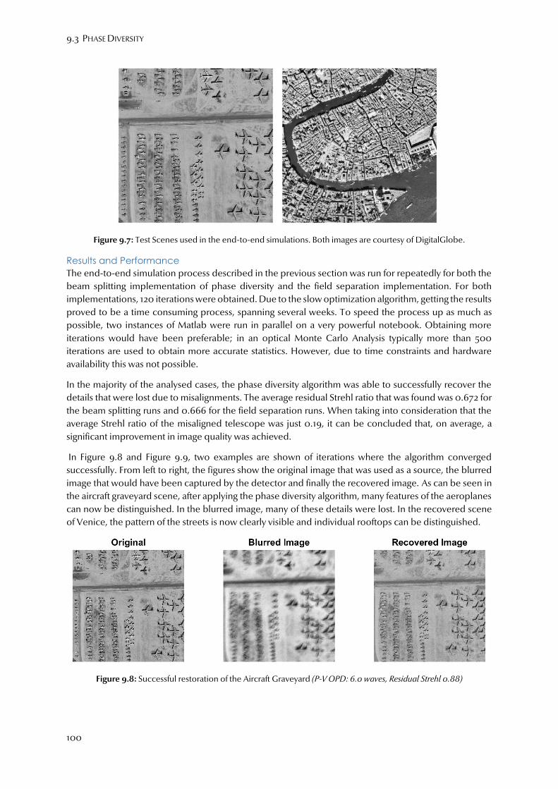
9.3 PHASE DIVERSITY

100

Figure 9.7: Test Scenes used in the end-to-end simulations. Both images are courtesy of DigitalGlobe.

Results and Performance

The end-to-end simulation process described in the previous section was run for repeatedly for both the

beam splitting implementation of phase diversity and the field separation implementation. For both

implementations, 120 iterations were obtained. Due to the slow optimization algorithm, getting the results

proved to be a time consuming process, spanning several weeks. To speed the process up as much as

possible, two instances of Matlab were run in parallel on a very powerful notebook. Obtaining more

iterations would have been preferable; in an optical Monte Carlo Analysis typically more than 500

iterations are used to obtain more accurate statistics. However, due to time constraints and hardware

availability this was not possible.

In the majority of the analysed cases, the phase diversity algorithm was able to successfully recover the

details that were lost due to misalignments. The average residual Strehl ratio that was found was 0.672 for

the beam splitting runs and 0.666 for the field separation runs. When taking into consideration that the

average Strehl ratio of the misaligned telescope was just 0.19, it can be concluded that, on average, a

significant improvement in image quality was achieved.

In Figure 9.8 and Figure 9.9, two examples are shown of iterations where the algorithm converged

successfully. From left to right, the figures show the original image that was used as a source, the blurred

image that would have been captured by the detector and finally the recovered image. As can be seen in

the aircraft graveyard scene, after applying the phase diversity algorithm, many features of the aeroplanes

can now be distinguished. In the blurred image, many of these details were lost. In the recovered scene

of Venice, the pattern of the streets is now clearly visible and individual rooftops can be distinguished.

Figure 9.8: Successful restoration of the Aircraft Graveyard (P-V OPD: 6.0 waves, Residual Strehl 0.88)

9.3 PHASE DIVERSITY

101

Figure 9.9: Successful restoration of Venice (P-V OPD: 4.4 waves, Residual Strehl: 0.94)

Not all iterations were successful, however. Recovered Strehl ratios higher than 0.80 were only obtained

in 66% and 63% of the iterations for, respectively, the beam splitting method and the field separation

method. In approximately 25 % of the cases, no improvement was observed or artefacts were too strong

for the image to be useful.

In Figure 9.10, the residual Strehl ratios of all iterations have been plotted against the P-V wavefront error

and the Strehl ratio of the misaligned system. In addition, some iterations have been added that were

obtained with an alignment budget that is a factor two less tight. As can be seen, the iterations are

clustered together in two main groups. Either the image restoration was successful and a high residual

Strehl ratio (>0.80) was obtained, or the algorithm failed and the Strehl ratio stays below a value of 0.30.

Intermediate Strehl ratios are slightly more common for the field separation method, but on the whole,

such values are relatively rare. It is also clear that the convergence ratio for the loose alignment budget is

very poor, making it very clear that such a budget is definitely not an option.

Figure 9.10: Residual Strehl ratio of all iterations plotted against the P-V wavefront error and the Strehl Ratio of the

misaligned system (𝜆 = 450 nm)

The failure of the algorithm to converge can be attributed to two factors. First of all, to save time, the total

number of iterations is limited to 250. For field separated phase diversity, this number was later increased

to 400, as it was found that the rate of convergence was slightly slower for this method. Usually, within

this number of iterations, the algorithm is either very close to its optimum or has become stuck at a local

minimum. However, in some cases, the error metric is still descending when the optimization process is

cut short.

Thus, the Strehl ratios obtained for these iterations are overly pessimistic. Iterations for which the

optimization process was cut short are typically found in the intermediate ranges. A second reason which

9.3 PHASE DIVERSITY

102

can explain a lack of convergence is the regularization method that has been used. The Reduced Gaussian

method is known to suffer from poor convergence when the SNR ratio is low. While a SNR ratio of 100 is

in itself not particularly low, noise amplification is more serious problem when large wavefront errors need

to be recovered.

It should be noted however, that while a high residual Strehl ratio often leads to a better quality, it is

certainly possible that even with a lower ratio the image quality is still good enough for many applications.

To find out for which residual Strehl ratio an acceptable image quality is obtained, images with a broad

variation in Strehl ratio were compared side by side. In Figure 9.11, on the next page, four of the images

that have been analysed are shown. The images have different residual Strehl ratios, ranging from 0.05 to

0.56.

When looking at the first image, with a residual Strehl ratio of 0.05, it is clear that this image is not suitable

for any application. The PSF that is recovered (on the right) does not look anything like the actual PSF. Very

strong artefacts are visible most details. At a Strehl ratio of 0.37, image quality has started to improve

considerably. However, there are still strong artefacts in the image, obscuring a lot of detail. As such, this

image quality

Figure 9.11: Image quality for four residual Strehl ratios

For Strehl ratios higher than 0.40, artefacts have mostly disappeared. While the retrieved and actual PSF

are still not identical, the difference have become substantially smaller. The image is not as sharp as one

that has a higher residual Strehl ratio, but with some additional sharpening are likely good enough for a

lot of applications, such as defence and security.

For a recovered Strehl ratio of 0.56, the difference between the recovered and actual PSF has become

hard to spot, even with the logarithmic scale used in the figure.

In Figure 9.12 and Figure 9.13, histograms are shown for the residual Strehl ratio that have been obtained

using beam splitting phase diversity and field separated phase diversity. Based on the findings presented

in Figure 9.11, iterations for which a Strehl ratio higher than 0.4o was obtained were considered to be

successful and are therefore coloured in green. In the figures it is shown that for both methods the majority

of the iterations was successful. Beam splitting phase diversity has a success ratio of 69%, while a ratio of

73% was obtained for field separated phase diversity.

9.4 FUTURE WORK

103

Figure 9.12: Histogram of the residual Strehl ratio for beam splitting phase diversity

Although the success ratio of field separated phase diversity is slightly higher, this is partly the result of

using a larger number of iterations in the evaluation of this method. The residual Strehl ratio that is

obtained for the successful iterations is typically slightly lower. Unlike with the beam splitting method,

there is a substantial number of iterations falling within the 0.4 – 0.7 range. It can therefore be concluded

that beam splitting phase diversity works slightly better than field separated phase diversity. However, the

gain in light that results from the second, more than compensates its slightly lower phase diversity

performance.

Figure 9.13: Histogram of the residual Strehl ratio for field splitting phase diversity

9.4. Future Work

In this chapter, phase diversity algorithms have been demonstrated that can successfully recover the

unknown wavefront error and restore the image. There is still a lot of room for improvements to these

algorithms, however. Future work on this topic will be focussed on two main points. First of all, the speed

and stability of the algorithms will be addressed to ensure that more accurate results can be obtained

within a shorter time span. Secondly, there a will be a focus on the easing of the simplification listed in

Section 9.3.2.

9.4 FUTURE WORK

104

9.4.1. Speed and Stability

Although the algorithms could successfully recover the wavefront in the majority of the cases, in more

than a quarter of the cases, the algorithms got stuck at a local minimum. Also, the computing times were

very long, which makes running the simulations a very time consuming process.

A number of steps can be taken to address these issues, listed below:

Derivation of an analytical gradient function: Currently, the gradients used in the non-linear

optimization algorithm are obtained by using a finite differences approach. This approach uses a

lot of system resources and has a limited accuracy. It possible to derive an analytical gradient

function. Such a gradient function can be computed much faster and is more accurate.

Implementation of better regularization schemes: To regularize the problem, at the moment

the Reduced Gaussian method is used. While this method is easy to implement, more stable

convergence is typically reached with more advanced phase diversity methods. The Multiframe

Wiener Filter Regularization method is a promising candidate to be implemented in the

algorithms.

Better integration with interferometric metrology system: The interferometric metrology

system, described in the thesis of Saish Sridharan, is currently only used to correct for deployment

errors as well as long term drifts. Provided that the accuracy of the system is sufficient, it can also

be used to obtain a first order estimate of the wavefront error. Using this wavefront error as a

starting point in the phase diversity calculations will result in a significant reduction in run time. In

addition, the risk of running into local minima is reduced.

Better use of available hardware: A simulation program which makes better use of hardware

capabilities can result in a much faster runtime.

To some extent, the last point in the list was already addressed. By using GPU Acceleration offered in the

Parallel Computing toolbox of Matlab, it was possible to reduce run times by an order of magnitude.

Performing the calculations on the GPU (Graphical Processer Unit) instead of the CPU works very well,

since the algorithm is highly parallelisable. In Figure 9.14, a comparison between performing the

calculations on the CPU and GPU is shown. The figure shows the run time needed for the optimization of

10 Zernike terms for 250 iterations. Thanks to the GPU acceleration, a run time of 3180 seconds on a very

capable six core processor can be brought back to 330 seconds on a GPU device. With some additional

code optimizations it can even be brought back to 290 seconds; a performance gain of more than a factor

10.

Figure 9.14: Performance comparison between performing calculations on the CPU and GPU.

Moving away from Matlab towards a programming language that has less overhead can result in additional

processing speed gains. The gains are expected to be limited, since as it is, the program already avoids

well known weaknesses of Matlab, such as for-loops. Furthermore, implementing proper Multi core

performance and GPU acceleration in another programming language will be challenging.

9.4 FUTURE WORK

105

9.4.2. Sampling, Detector MTF and Other Blur Sources

To simplify the model, several assumptions have been made with respect to the sampling and the detector

MTF. It was assumed that the intensity pattern is Nyquist sampled and that the detector has no influence

on the MTF. In reality, it will be very hard to create a system with which Nyquist sampling can be achieved,

however, as demonstrated by Eq.(9.15) [109]:

𝑓/# ≥𝑄𝑑𝑝𝑖𝑥𝑒𝑙

𝜆 (9.15)

Where 𝑓/# is the f/number of the system and 𝑑𝑝𝑖𝑥𝑒𝑙 is the detector pixel pitch. 𝑄 is a parameter describing

the sampling rate. When the value is larger or equal to 1, the field is adequately sampled. If the value is

larger or equal to 2, the intensity pattern is Nyquist sampled. With a pixel pitch of 5.5 micron and an

f/number of 8, it can be shown that the sampling rate of the deployable telescope is 0.65 for the shortest

wavelength of 450 nm. It can therefore be concluded that the image is undersampled. An adequately

sampled image would require an f/number of at least f/12, which would result in substantial loss of light

on the detector.

Despite this, phase diversity algorithms can still be used. Although these algorithms are no longer able to

retrieve fine features of the PSF, it can still retrieve larger features that are dictated by geometrical optics.

Since these features have the most profound effect on the image quality, the algorithms can still be

successfully applied to restore the image [110] . In [111] it is shown that for sampling ratios as low as 0.60,

the loss in performance of the algorithms is small.

Blur sources, such as detector crosstalk, ground smear and spacecraft jitter, are currently ignored. In future

of the model, these issues should also be addressed. These issues can either be corrected separately, or

included in the optimization. Detector MTF can vary from sample to sample, so it is probably best to

correct detector crosstalk separately, prior to using the images in the phase diversity algorithms. The

correction can be based on on-ground characterization of the detector. Factors such as spacecraft jitter

and ground smear, on the other hand, can be included in the optimization, since they will be the same for

both detectors.

9.4.3. Chromatic Light and Field Dependence

In the current model, the PSF is assumed to be independent of the wavelength as well as the field. In reality

this is not the case. It is however, not expected that either issue will lead to problems in the future.

As shown in [112], the assumption of monochromatic light still leads to acceptable results up to a

bandwidth of 100 nm. For wider bands, a grey world assumption can be made (i.e. the spectrum of the

scene is assumed to be flat). Using the grey world assumption, Strehl ratios higher than 0.80 can be

achieved for wavebands as wide as 100% of the central wavelength [112]. Since the central wavelength of

the deployable telescope is 550 nm, chromatic effects are unlikely to limit the broadband performance

of the instrument.

Additional research is needed to assess the impact of the field dependence of the PSF. The phase diversity

algorithms only analyse a small section of the image at a time. As demonstrated by the PSF in Figure 9.15,

the wavefront varies only slightly across the whole swath width. The three PSF are almost identical,

indicating that the wavefront is almost the same for the whole FOV. Since the width of the analysis region

is only 500 pixels in width, a fraction of the 20,800 pixel swath, the effect is expected to be negligible.

9.4 FUTURE WORK

106

Figure 9.15: PSFs for the central and extreme field angles

It is important to realize, however, that at moment, other than a radius change, possible deformations of

the mirror segments are not included in the models. Although it is not expected, it is possible that

including these errors will increase the spatial variation.

107

10. Conclusions and Recommendations

In this chapter, an overview will be given of the conclusions that can be drawn based on the work in this

thesis. In section 10.1, the conclusions of this thesis will be presented, while section 10.2 provides an

overview of future work that can be done to improve the design.

10.1. Conclusions

In this thesis a design for a deployable telescope was presented that can reach a ground sampling distance

of 25 cm from an altitude of 500 km. With a stowed volume of 0.363 m3 and a nominal mass of 74.8 kg,

the design is expected to be substantially smaller and lighter than state-of-the-art systems such as

GeoEye-2 and Worldview-3. The design is the result of a concept study for which two optical designs were

created; a Michelson synthetic aperture and a Fizeau synthetic aperture.

The Michelson system, first of all, consists of 12 afocal telescopes spread in an annular pattern across the

1.5 meter pupil plane. The outgoing beams of these telescopes are steered towards a beam combiner

which focusses all the light in a common focal plane. The afocal telescopes consist of three aspherical

mirrors, aimed at providing a diffraction limited wavefront quality with the appropriate amount of sine-

law distortion. The latter is needed to ensure that the wavefront quality in the corners can be met. The

complete system offers a diffraction limited image quality in the centre. A slight performance degradation

can be observed at the edges of the field of view, where the MTF at the Nyquist frequency is 3% lower than

the diffraction limited MTF.

The Fizeau system is based on a Full-Field Korsch Three Mirror Anastigmat (TMA). The primary mirror has

been replaced by three rectangular mirror panels placed in a tri-arm configuration. The system offers a

diffraction limited performance that is consistent across the complete field of view.

In a trade-off, it was determined that the Fizeau system is most suitable for Earth Observation from a Low

Earth Orbit platform. It was selected based on smaller stowed volume, a higher MTF, a larger aperture

area, a lower complexity and a better thermo-mechanical stability. Only in terms of the straylight

sensitivity, the Michelson system is slightly better, thanks to its small telescopes that are easier to baffle.

In a tolerance analysis, it was shown that the telescope is very sensitive to misalignments of the primary

mirror segments. Even with displacements of a primary mirror segment by a distance of just 100

nanometre or a tilt of 0.2 microradians, the image quality is only acceptable if reconstruction algorithms

are applied. Such high accuracies can only be reached with a combination of a robust mechanical design,

which minimizes mechanical uncertainties, and a well thought out calibration strategy.

A preliminary mechanical design of the instrument was created using Catia. The rectangular mirror

segments will be made from Silicon Carbide, a material with a very high stiffness, a high conductivity and

a low coefficient of thermal expansion. Triangular pockets will be cut into the back of the mirror segment,

to ensure that a low areal density of 10 kg/m2 can be achieved. The segments will be connected to the

moving support frame using a whiffle-tree assembly. This approach reduces stress concentrations at the

fastening points, without overconstraining the element. In addition, it can counter the bending of the

mirror segment under the influence of its own gravity, which can occur during on-ground testing. Between

the whiffles and the frame, actuators can be placed to correct the piston and tilt error of the mirror

segments.

The secondary mirror assembly will be connected to the main housing via three foldable arms. This

approach is similar to the conceptual design of the International X-ray Observatory (IXO) mission. The

arms will be made of Invar, a metal with a low coefficient of thermal expansion.

10.2 FUTURE WORK

108

For the in-orbit calibration, a two stage calibration procedure is proposed. First of all, following the follows

the launch and deployment, a coarse calibration procedure is started. This system uses a combination of

interferometric measurements and cpacitive sensors to determine the offsets of each of the optical

elements. The knowledge that is obtained using these systems, can be used to correct the mirror postions

using actuators. If necessary, the metrology system may be supplemented with phase retrieval algorithms

that are based on the analysis of star images that are obtained with the telescope. An analysis of such an

algorithm is the Gerchberg-Saxton algorithm. A more detailed analysis of the metrology systems that can

be used during this calibration phase can be found in the thesis of Saish Sridharan.

Once the peak-to-valley wavefront error has been reduced to a value of 7 waves or lower, a passive phase

diversity system can retrieve the remaining wavefront error and use it to reconstruct the image. As an input

to the algorithm, two images are needed. One of those should be obtained with a detector placed in the

nominal focus of the system while the second detector should be intentionally defocussed by a known

distance.

In an end-to-end model, phase diversity algorithms have been tested for a wide variety of different offsets

that can occur if the alignment budget in Table 7.3 is met. Two different implementations of phase diversity

were tested. In the first implementation, a beamsplitter is placed in the beam to ensure that both detectors

will receive light. In the second approach, the two detectors look at a slightly different field separated in

the along-track direction.

It was found that both implementations lead to very similar results. In 69% of the analysed cases, the

beamsplitting implementation was able to successfully recover the wavefront and improve the image. For

field separated phase diversity, a success rate of 73% was obtained. Recovered Strehl ratios higher than

0.80 (the diffraction limit) were obtained in 66% and 63% of the analysis cases for, respectively, the beam

splitting method and the field separation method. It is expected that with further refinement of the

algorithms, these percentages can be increased significantly, so that the system will be able to offer a

diffraction limited image quality in almost all operating conditions.

10.2. Future Work

In this thesis a lot of aspects regarding synthetic instruments have been discussed and analysed. However,

there remains a lot of work that can be done. In this section several topics are listed which will require

additional research. These topics will likely be a part of a PhD research project that will carry on the work

presented in this thesis.

Optical Design and Analysis: In terms of the nominal optical performance, the current design does not

leave a lot of room for improvement. However, as shown in Chapter 7, the design is very sensitive to

misalignments of the primary mirror segments, which makes the alignment and in-orbit calibration very

challenging. To some extent, this is the result of the small f-number of the Cassegrain part of the TMA. By

increasing this f-number, the alignment sensitivity will be reduced. Doing so will increase the length of the

deployable boom, which increases the uncertainty in the position of the secondary mirror. However,

since misalignments of the primary mirror segments turned out to be dominant over misalignments of the

secondary mirror, the change should lead to an overall reduction in sensitivity of the system.

Additional optical analysis should also be devoted to the straylight, an important issue for deployable

telescopes. Since the optical elements of a deployable telescope are not enclosed in the housing structure

of the instrument, the system is inherently more sensitive to straylight. In a straylight analysis, it should be

analysed whether or not straylight will lead to any issues and how these issues can be resolved. It is

foreseen that the telescope will need a deployable baffle which will shield the primary mirror segments.

Mechanical Design and Analysis: The mechanical design is still in a conceptual design phase and a lot of

additional design and analysis work is still required. Several components of the design, such as the main

10.2 FUTURE WORK

109

housing, the mirror mounts, the deployment mechanisms and the actuation systems need to be designed

in more detail. Furthermore, (thermo-)mechanical analyses should be done on the system to assess the

impact of thermal fluctuations, platform vibrations, launch loads and gravity release effects. A finite

element model of the complete system and individual components must be created to allow further

optimisation of the mechanical design.

Calibration and Image Processing: In terms of the calibration system and the image processing

algorithms there is still a lot of work that can be done. The metrology system, that can measure offsets of

the mirrors during the post-launch calibration phase, must be worked out in more detail and the actuator

and control systems must still be designed. A lot of refinement is still possible in the phase diversity

algorithms that have been used. On the one hand, several assumptions that are currently made must be

relaxed. The model should be adapted to properly analyse polychromatic light and additional blurring

due to detector convolution should be taken into account. In addition, several refinements can be made

to improve the performance and stability of the algorithms. A more complete overview of refinements

that are needed can be found in Section 9.4.

111

Bibliography

1. Kuiper, J.M. and J. Bouwmeester, A 1.5U Cube-Sat Camera Cornerstone Design for a Multiple Aperture Earth

Observation System. IAC Capetown Conference Proceedings, 2011.

2. Kuiper, J.M. and D. Dolkens, ANT-2 and ARCTIC-1 Cube-Sat Camera Cornerstone Designs for Earth

Observation. International Astronautical Congress 2012, Naples, 2012.

3. Kuiper, J.M. and D. Dolkens, Cube-Sat Constellation Designs for EO Systems. 9th IAA Symposium on Small

Satellites for Earth Observation, 2013.

4. Airbus Defence & Space. Satellite Imagery - The Constellation. 2014 20-11-2014]; Available from:

http://www.geo-airbusds.com/en/65-satellite-imagery.

5. Digital Globe. Worldview 3, Above+Beyond. 2014, 22-11-2014]; Available from:

http://worldview3.digitalglobe.com/.

6. Corporation, S.I. Satellite Sensors. 2014 22-11-2014]; Available from:

http://www.satimagingcorp.com/satellite-sensors/.

7. Davies, P., et al., The DMC-3 1m Small Satellite Constellation, in 8th IAA Symposium on Small Satellites for

Earth Observation. 2011: Berlin.

8. Ferster, W. DigitalGlobe Adding Infrared Capability to Worldview-3 Satellite. Space News 2012; Available

from: http://www.spacenews.com/article/digitalglobe-adding-infrared-capability-worldview-3-

satellite.

9. Selding, P.B.d. Astrium Services Girds for Competition with DigitalGlobe-GeoEye Combo. 2012 20-11-2014];

Available from: http://earsc.org/news/astrium-services-girds-for-competition-with-digitalglobe-

geoeye-combo.

10. Shalal, A. DigitalGlobe gains U.S. govt license to sell sharper satellite imagery. 2014 20-11-2014]; Available

from: http://www.reuters.com/article/2014/06/11/digitalglobe-imagery-idUSL2N0OR2UX20140611.

11. Bolcar, M.R., Phase diversity for segmented and multi-aperture systems. 2009: ProQuest.

12. Brouard, L., et al., Optical Aperture Synthesis: Limitations and Interest for the Earth Observation, in Sixth

International Conference on Space Optics. 2006: Noordwijk, The Netherlands.

13. Chang, C.-I., Hyperspectral data exploitation: theory and applications. 2007: John Wiley & Sons.

14. Green, R.O., S. Hook, and B. Middleton, HyspIRI Draft Preliminary Level 1 Requirements, NASA, Editor. 2010.

15. GeoEye, GeoEye-1 Instrument/Product Description. 2009.

16. Materne, A. Backthinned TDI CCD Image Sensor Design and Performances for the Pleiades High Resolution

Earth Observation Satellites. in ESA Special Publication. 2006.

17. Tyson, R.K., Introduction to Adaptive Optics: Robert K. Tyson. 2000: SPIE Press.

18. Barnhart, D. and M. Sweeting, Right-sizing Small Satellites. 2014.

19. Stubbs, D.M., et al. Multiple instrument distributed aperture sensor (MIDAS) science payload concept. in

Astronomical Telescopes and Instrumentation. 2004. International Society for Optics and Photonics.

20. CVI Melles Griot, All Things Photonic, The CVI Melles Griot Technical Guide. Vol. 2. 2009.

21. Hecht, E., Optics. 2002: Pearson Education.

22. Teledyne Dalsa, Piranha HS HS-S0-12Kxx. 2011.

23. He, X.-F. and N. O, Time Delay Integration speeds up imaging. Photonics Spectra, 2012. 46(5): p. 50.

24. Hamamatsu, TDI-CCD image sensors. 2014.

25. Yu, H., et al. A time-delay-integration CMOS image sensor with pipelined charge transfer architecture. in

Circuits and Systems (ISCAS), 2012 IEEE International Symposium on. 2012. IEEE.

26. Fairchild Imaging, Data Sheet Fairchild Imaging CCD 21241. 2013.

27. Anomet, Technical Data Sheet: Anolux MIRO Silver - 27 AG. 2004.

28. Smith, W.J., Modern Optical Engineering. 2008: McGraw-Hill.

29. Weisstein, E.W. Zernike Polynomial. MathWorld - A Wolfram Web Resource 2013 14-3-2013]; Available

from: http://mathworld.wolfram.com/ZernikePolynomial.html.

30. Wyant, J.C. and K. Creath, Basic Wavefront Aberration Theory for Optical Metrology, in Applied Optics and

Optical Engineering. 1992, Academic Press.

31. Mahajan, V.N. and G.-m. Dai, Orthonormal polynomials in wavefront analysis: analytical solution. Journal of

the Optical Society of America, 2007. 24(9): p. 2994-3016.

http://www.geo-airbusds.com/en/65-satellite-imagery

http://worldview3.digitalglobe.com/

http://www.satimagingcorp.com/satellite-sensors/

http://www.spacenews.com/article/digitalglobe-adding-infrared-capability-worldview-3-satellite

http://www.spacenews.com/article/digitalglobe-adding-infrared-capability-worldview-3-satellite

http://earsc.org/news/astrium-services-girds-for-competition-with-digitalglobe-geoeye-combo

http://earsc.org/news/astrium-services-girds-for-competition-with-digitalglobe-geoeye-combo

http://www.reuters.com/article/2014/06/11/digitalglobe-imagery-idUSL2N0OR2UX20140611

http://mathworld.wolfram.com/ZernikePolynomial.html

112

32. Mahajan, V.N., Zernike annular polynomials for imaging systems with annular pupils. Journal of the Optical

Society of America, 1984. 1: p. 685.

33. Shaw-McMinn, P.G. How to Provide High-Resolution Vision. 2006 14-3-2013]; Available from:

http://cms.revoptom.com/index.asp?ArticleType=SiteSpec&Page=osc/105418/lesson.htm.

34. Goodman, J.W., Introduction to Fourier Optics. 1996: McGraw-Hill.

35. MIT OpenCourseWare. Spatially Incoherent Imaging. 2009 17-4-2013]; Available from:

http://ocw.mit.edu/courses/mechanical-engineering/2-71-optics-spring-2009/video-lectures/lecture-

22-coherent-and-incoherent-imaging/MIT2_71S09_lec22.pdf.

36. Goodman, J.W., Statistical Optics. 2000: Wiley Classics Library.

37. Mashaal, H., et al., First direct measurement of the spatial coherence of sunlight. Optical Letters, 2012. 37: p.

3516-3518.

38. Voelz, D.G., Computational fourier optics: a MATLAB tutorial.

39. Boreman, G.D., Modulation Transfer Function in Optical and Electro-Optical Systems. 2001, Bellingham, WA:

SPIE Press.

40. Beckers, J., B. Ulich, and J. Williams. Performance of the Multiple Mirror Telescope (MMT) I. MMT-the first of

the advanced technology telescopes. in 1982 Astronomy Conferences. 1982. International Society for Optics

and Photonics.

41. Zarifis, V., et al. The multi aperture imaging array. in Working on the Fringe: optical and IR interferometry from

ground and space. 1999.

42. Mugnier, L., et al. Continuous High-Resolution Earth Observation with Multiple Aperture Optical Telescopes.

in Proceedings of the OPTRO 2005 International Symposium. 2005.

43. Cassaing, F., et al. Optical design of a Michelson wide-field multiple-aperture telescope. in Optical Systems

Design. 2004. International Society for Optics and Photonics.

44. Golay, M.J.E., Point Arrays Having Compact, Nonredundant Autocorrelations. J. Opt. Soc. Am., 1971. 61(2): p.

272-273.

45. Chung, S.-J. and D. Miller, Design, Implementation and Operation of a Sparse Aperture Imaging Satellite.

2002.

46. Blanc, P., F. Falzon, and E. Thomas, A new concept of synthetic aperture instrument for high resolution earth

observation from high orbits. 2005, DTIC Document.

47. Harvey, J.E. and C. Ftaclas. Fundamental limitations on off-axis performance of phased telescope arrays. in

Astronomy'90, Tucson AZ, 11-16 Feb 90. 1990. International Society for Optics and Photonics.

48. Labeyrie, A., Hypertelescopes: The Challenge of Direct Imaging at High Resolution. EAS Publications Series,

2013. 59: p. 5-23.

49. Stuhlinger, T.W. All-reflective phased array imaging telescopes. in 1990 Intl Lens Design Conf. 1991.

International Society for Optics and Photonics.

50. Golay, M.J., Point arrays having compact, nonredundant autocorrelations. JOSA, 1971. 61(2): p. 272-273.

51. Liu, L., et al., Novel array configuration and its optimization for sparse aperture imaging systems. Optical

Engineering, 2011. 50(5): p. 053202-053202-7.

52. Jones, L., Reflective and Catadioptric Objectives, in Handbook of Optics, M. Bass and V.N. Mahajan, Editors.

2010, Optical Society of America.

53. Korsch, D., Reflective optics. 1991: Academic Press.

54. Pitman, J.T., et al. Remote sensing space science enabled by the multiple instrument distributed aperture sensor

(MIDAS) concept. in Optical Science and Technology, the SPIE 49th Annual Meeting. 2004. International

Society for Optics and Photonics.

55. Grogan, R.L., G.H. Blackwood, and R.J. Calvet. Optical delay line nanometer-level pathlength control law

design for space-based interferometry. in Astronomical Telescopes & Instrumentation. 1998. International


56. Contreras, J.W. and P.A. Lightsey. Optical design and analysis of the James Webb Space Telescope: optical

telescope element. in Optical Science and Technology, the SPIE 49th Annual Meeting. 2004. International


57. Underwood, C. and S. Pellegrino, Autonomous Assembly of a Reconfigurable Space Tele-scope (AAReST) for

Astronomy and Earth Observation.

58. Glaser, I. and E. Chernyak. Optical micro-satellite telescopes using a synthetic aperture approach for improved

resolution. in SPIE Optical Engineering+ Applications. 2010. International Society for Optics and Photonics.

http://cms.revoptom.com/index.asp?ArticleType=SiteSpec&Page=osc/105418/lesson.htm

http://ocw.mit.edu/courses/mechanical-engineering/2-71-optics-spring-2009/video-lectures/lecture-22-coherent-and-incoherent-imaging/MIT2_71S09_lec22.pdf

http://ocw.mit.edu/courses/mechanical-engineering/2-71-optics-spring-2009/video-lectures/lecture-22-coherent-and-incoherent-imaging/MIT2_71S09_lec22.pdf

113

59. Huybrechts, S., et al. Structural design for deployable optical telescopes. in Aerospace Conference Proceedings,

2000 IEEE. 2000. IEEE.

60. Catanzaro, B.E., et al. UltraLITE glass/composite hybrid mirror. in Astronomical Telescopes and

Instrumentation. 2000. International Society for Optics and Photonics.

61. da Silva Curiel, A., et al., First year in orbit–results from the Beijing-1 operational high resolution small satellite,

in Small Satellites for Earth Observation. 2008, Springer. p. 357-364.

62. Dierickx, P., et al. The optics of the OWL 100-m adaptive telescope.

63. Tsuneta, S., K. Ichimoto, and et al, The Solar Optical Telescope for the Hinode Mission: An Overview. Solar

Physics, 2008. 249: p. 167-196.

64. Korsch, D., Anastigmatic three-mirror telescope. Appl. Opt., 1977. 16(8): p. 2074-2077.

65. Laureijs, R., Definition Study Report: Euclid, Mapping the geometry of the dark Universe. 2011.

66. Howard, J.M., K.Q. Ha, and et al, Optical Modeling Activities of NASA's James Webb Space Telescope (JWST):

V. Operational Alignment Updates. Proceedings of SPIE, 2008. 7017.

67. Lampton, M. and M. Sholl, Comparison of On-Axis Three-Mirror Anastigmat Telescopes. Proceedings of SPIE

- International Society for Optical Engineering, 1999. 6687.

68. Taccola, M., et al. The cryogenic refocusing mechanism of NIRSpec opto-mechanical design, analysis, and

testing. in SPIE Astronomical Telescopes+ Instrumentation. 2008. International Society for Optics and

Photonics.

69. Peterson, L.D., J.D. Hinkle, and S. Ismail. Deployable optics for Earth observing lidar instruments. in Earth

Science Technology Conference Proce. NASA ESTO Earth Science Technology Conference, Palo Alto, CA. 2004.

70. Nella, J., et al. James Webb Space Telescope (JWST) observatory architecture and performance. in Astronomical

Telescopes and Instrumentation. 2004. International Society for Optics and Photonics.

71. Castro, J., et al. Status of the design and fabrication of the GTC mirrors. in Astronomical Telescopes and


72. Podger, N.E. Overview of Image Quality Performance of the GeoEye-1 High Resolution Imaging Satellite. in 11th

Annual JACIE (Joint Agency Commercial Imagery Evaluation) Workshop. 2012. Fairfax, VA, USA.

73. Edmund Optics. Understanding Optical Specifications. 2014; Available from:

http://www.edmundoptics.com/technical-resources-center/optics/understanding-optical-

specifications.

74. Gielesen, W., et al. Gaia basic angle monitoring system. in SPIE Optical Engineering+ Applications. 2013.


75. Stahl, H.P., D.T. Leisawitz, and D.J. Benford. Mirror requirements for SAFIR. in Astronomical Telescopes and


76. Johnson, J.S., K.D. Grobsky, and D. Bray. Rapid fabrication of lightweight silicon-carbide mirrors. in

International Symposium on Optical Science and Technology. 2002. International Society for Optics and

Photonics.

77. Weber, M.J., Handbook of Optical Materials. 2002: Taylor & Francis.

78. Stahl, H.P., L.D. Feinberg, and S.C. Texter. JWST primary mirror material selection. in Astronomical Telescopes

and Instrumentation. 2004. International Society for Optics and Photonics.

79. Steinkopf, R., et al. Metal mirrors with excellent figure and roughness. in Optical Systems Design. 2008.


80. Gubbels, G., L. Tegelaers, and R. Senden. Melt spun aluminium alloys for moulding optics. in SPIE Optifab.

2013. International Society for Optics and Photonics.

81. Baiocchi, D. and H.P. Stahl, Enabling future space telescopes: mirror technology review and development

roadmap. astro2010: The Astronomy and Astrophysics Decadal Survey, Technology Development Paper,

2009(23).

82. Ruffner, J.A., et al. Fabrication and characterization of beryllium-based multilayer mirrors for soft x-rays. in San

Diego,'91, San Diego, CA. 1992. International Society for Optics and Photonics.

83. Parsonage, T.B. JWST beryllium telescope: material and substrate fabrication. in Astronomical Telescopes and


84. Egerman, R., The Current and Future State-of-the-art Glass Optics for Space-based Astronomical Observatories.

2010.

85. Schott, Zerodur - Zero Expansion Glass Ceramic. 2014.

http://www.edmundoptics.com/technical-resources-center/optics/understanding-optical-specifications

http://www.edmundoptics.com/technical-resources-center/optics/understanding-optical-specifications

114

86. Hobbs, T.W., M.J. Edwards, and R.R. VanBrocklin. Current fabrication techniques for ULE and fused silica

lightweight mirrors. in Proceedings of SPIE. 2003.

87. Vargas, H.S., SiC Design Guide: Manufacture of Silicon Carbide Products (Briefing charts). 2010, DTIC

Document.

88. Northrop Grumman. Silicon Carbide. 2014.

89. Harnisch, B., et al., Ultra-lightweight C/SiC mirrors and structures. ESA bulletin, 1998. 95(8): p. 148-152.

90. Matson, L.E., et al., Silicon carbide technologies for lightweighted aerospace mirrors. 2008, DTIC Document.

91. Breysse, J., D. Castel, and M. Bougoin, All-SiC telescope technology at EADS-Astrium. Proc. ICSO (6c-022),

2012.

92. Lake, M.S., et al., A deployable primary mirror for space telescopes. 1999: National Aeronautics and Space

Administration, Langley Research Center.

93. Gallagher, B., et al. JWST mirror production status. in SPIE Optical Engineering+ Applications. 2011.


94. Dimmler, M., et al. E-ELT primary mirror control system. in SPIE Astronomical Telescopes+ Instrumentation.

2008. International Society for Optics and Photonics.

95. Nijenhuis, J., R. Hamelinck, and B. Braam. The opto-mechanical performance prediction of thin mirror

segments for E-ELT. in SPIE Astronomical Telescopes+ Instrumentation. 2012. International Society for Optics

and Photonics.

96. European Space Agency, IXO: The International X-ray Observatory. ESA Yellow book, Draft 0.4, 2010.

97. Lake, M.S. and M.R. Hachkowskil, Mechanism design principles for optical-precision, deployable instruments.

2000.

98. Lake, M.S., P.A. Warren, and L.D. Peterson. A revolute joint with linear load-displacement response for

precision deployable structures. in 37th AIAA/ASME/ASCE/AHS/ASC Structures, Structural Dynamics, and

Materials Conference, Salt Lake City, Utah. 1996.

99. Kim, Y., et al. Nuclear Spectroscopic Telescope Array (NuSTAR) Mission. in Aerospace Conference, 2013 IEEE.

2013. IEEE.

100. Laureijs, R., et al. Euclid: ESA's mission to map the geometry of the dark universe. in SPIE Astronomical

Telescopes+ Instrumentation. 2012. International Society for Optics and Photonics.

101. Gerchberg, R. and W. Saxton, A practical algorithm for the determination of phase from image and diffraction

plane pictures. SPIE milestone series MS, 1994. 94: p. 646-646.

102. Fienup, J.R., Phase retrieval algorithms: a comparison. Applied optics, 1982. 21(15): p. 2758-2769.

103. Paxman, R. and J. Fienup, Optical misalignment sensing and image reconstruction using phase diversity. JOSA

A, 1988. 5(6): p. 914-923.

104. Paxman, R.G., T.J. Schulz, and J.R. Fienup, Joint estimation of object and aberrations by using phase diversity.

JOSA A, 1992. 9(7): p. 1072-1085.

105. Gonsalves, R.A., Phase retrieval and diversity in adaptive optics. Optical Engineering, 1982. 21(5): p. 215829-

215829-.

106. Blanc, A., L.M. Mugnier, and J. Idier, Marginal estimation of aberrations and image restoration by use of phase

diversity. JOSA A, 2003. 20(6): p. 1035-1045.

107. Paxman, R.G., et al., Evaluation of phase-diversity techniques for solar-image restoration. The Astrophysical

Journal, 1996. 466: p. 1087.

108. Fienup, J.R., et al. Comparison of reconstruction algorithms for images from sparse-aperture systems. in

International Symposium on Optical Science and Technology. 2002. International Society for Optics and

Photonics.

109. Brady, G.R., M. Guizar-Sicairos, and J.R. Fienup, Optical wavefront measurement using phase retrieval with

transverse translation diversity. Optics express, 2009. 17(2): p. 624-639.

110. Fienup, J., Phase retrieval for undersampled broadband images. JOSA A, 1999. 16(7): p. 1831-1837.

111. Thurman, S.T. and J.R. Fienup, Complex pupil retrieval with undersampled data. JOSA A, 2009. 26(12): p.

2640-2647.

112. Bolcar, M.R. and J.R. Fienup. Phase diversity with broadband illumination. in Adaptive Optics: Methods,

Analysis and Applications. 2007. Optical Society of America.

115

Appendix A: Tighter Alignment Budget

In this Appendix, a tighter alignment budget is defined that will enable direct diffraction limited imaging

with the deployable telescope presented in this thesis. As shown in Table A.1, the alignment tolerances

are extremely tight, in particular the displacement in the z-direction of the primary mirror segments. In

this direction, a displacement of just 10 nm can be allowed. It is clear that meeting this budget will be very

challenging, if at all possible.

A near diffraction limited image quality is demonstrated in the histograms in Figure A.1 and Figure A.2. The

majority of the analysed cases result in a Strehl ratio higher than 0.8, although the number of iterations

between 0.6 and 0.8 is still somewhat on the high side. With additional tweaking of the budget, it is

expected that the performance can be improved somewhat, without needing to tighten the tolerances on

the most critical elements.

Table A.1: Position, Tilt and Radius Tolerances of the Curved Mirrors for a P-V wavefront budget of 0.25 waves

Element Position [µm] Tilt [µrad] Radius [%]

X Y Z X Y Z

Primary Mirror Segments 0.1 0.2 0.01 0.02 0.04 0.45 0.0001

Secondary Mirror 0.4 0.4 0.2 1.7 1.7 50 0.0001

Tertiary Mirror 1 1 0.5 1.7 1.7 50 0.0001

Figure A.1: RMS Optical Path Difference for the alignment budget in Table A.1

Figure A.2: Strehl Ratio for the alignment budget in Table A.1

A Deployable Telescope for Sub-Meter Resolutions from ...

Documents

Transcript of A Deployable Telescope for Sub-Meter Resolutions from ...