University of California

Los Angeles

Electromagnetic Characterizations of Mesh Deployable Ka Band

Reflector Antennas for Emerging CubeSats

A thesis submitted in partial satisfaction

of the requirements for the degree

Master of Science in Electrical Engineering

by

Vignesh Manohar

2016

c© Copyright by

Vignesh Manohar

2016

Abstract of the Thesis

Electromagnetic Characterizations of Mesh Deployable Ka Band

Reflector Antennas for Emerging CubeSats

by

Vignesh Manohar

Master of Science in Electrical Engineering

University of California, Los Angeles, 2016

Professor Yahya Rahmat-Samii, Chair

CubeSats are a miniaturized class of satellites that are launched as secondary payloads,

offering the possibility of carrying out advanced space missions at affordable costs. Mechan-

ical constraints and limited power onboard have limited current antenna implementations

to low-gain, low data rate, and near-omnidirectional patterns. Integrating high gain aper-

ture antennas with CubeSats can offer innumerable possibilities for advanced space missions.

However, packaging large apertures into the small CubeSat form factor presents a formidable

challenge to the scientific community. This thesis investigates the potential of integrating a

1m offset mesh deployable reflector antenna system with a 2.5U (10cm×10cm×25cm) Cube-

Sat chassis for Ka band remote sensing or communications. Packaging such a large aperture

into the small 2.5U volume necessitates a completely customized reflector design for our

application. A detailed study of deployable umbrella mesh reflectors, RF analysis of various

reflector antenna configurations and feed design methodologies are included in this work.

These particular studies not only demonstrate the feasibility of the next high-gain antenna;

they mark a major milestone (a 1m antenna size) for CubeSats, which is among the largest

to be utilized for Ka band.

ii

The thesis of Vignesh Manohar is approved.

Tatsuo Itoh

Benjamin Williams

Yahya Rahmat-Samii, Committee Chair

University of California, Los Angeles

2016

iii

I dedicate this thesis to my grandparents, who continue to guide me from above.

iv

Table of Contents

1 Introduction . . . . . . . . . . . . . . . . . . . . . . . . . . . . . . . . . . . . . . 1

1.1 Antennas for CubeSats: Current state of art . . . . . . . . . . . . . . . . . . 3

1.2 Reflector antennas for CubeSats: Past and future work . . . . . . . . . . . . 6

1.2.1 Focus of thesis . . . . . . . . . . . . . . . . . . . . . . . . . . . . . . 7

1.3 Organization of work . . . . . . . . . . . . . . . . . . . . . . . . . . . . . . . 9

2 Efficiencies for a Reflector Antenna System . . . . . . . . . . . . . . . . . 11

2.1 A discussion on efficiencies . . . . . . . . . . . . . . . . . . . . . . . . . . . . 11

2.2 Aperture efficiency: spillover and taper . . . . . . . . . . . . . . . . . . . . . 13

2.3 Efficiency for umbrella reflector antennas . . . . . . . . . . . . . . . . . . . . 15

2.4 Efficiency for mesh reflector antennas . . . . . . . . . . . . . . . . . . . . . . 15

2.5 Feed positioning and efficiency . . . . . . . . . . . . . . . . . . . . . . . . . . 16

2.6 Blockages . . . . . . . . . . . . . . . . . . . . . . . . . . . . . . . . . . . . . 16

3 Characterization of Umbrella Reflector Antennas: Analysis of Gain Lossand Estimation of Optimal Feed Point . . . . . . . . . . . . . . . . . . . . . . . 17

3.1 Mathematical representation of the gore surface . . . . . . . . . . . . . . . . 18

3.2 Finding the optimum feed location . . . . . . . . . . . . . . . . . . . . . . . 19

3.2.1 Physical intuition behind the optimal feed location . . . . . . . . . . 21

3.2.2 Physical Optics approach . . . . . . . . . . . . . . . . . . . . . . . . . 22

3.2.3 Best fit approach . . . . . . . . . . . . . . . . . . . . . . . . . . . . . 23

3.2.4 Manual tuning of feed position . . . . . . . . . . . . . . . . . . . . . . 24

3.3 Results and discussions . . . . . . . . . . . . . . . . . . . . . . . . . . . . . . 25

3.4 Extending the best-fit paraboloid approach: Effects of feed amplitude taper 26

3.5 Aperture distribution and far field comparison . . . . . . . . . . . . . . . . . 28

3.5.1 Detailed study of an umbrella reflector with Ng = 15 . . . . . . . . . 29

3.5.2 Detailed far field discussion: grating lobes . . . . . . . . . . . . . . . 31

4 Mesh Characterization for Reflector Antenna Systems . . . . . . . . . . . 34

4.1 Simple wire grid model . . . . . . . . . . . . . . . . . . . . . . . . . . . . . . 34

4.1.1 Astrakhan’s formulation . . . . . . . . . . . . . . . . . . . . . . . . . 35

4.1.2 Relating transmission coefficients to gain loss . . . . . . . . . . . . . 37

v

4.1.3 Comparison of full wave simulation with the Astrakhan formulation . 38

4.2 Hard and soft contact . . . . . . . . . . . . . . . . . . . . . . . . . . . . . . . 40

4.3 Complex mesh modeling and equivalent wire grid model . . . . . . . . . . . 42

4.4 3D wire models . . . . . . . . . . . . . . . . . . . . . . . . . . . . . . . . . . 44

5 Selection of Reflector Antenna Configuration . . . . . . . . . . . . . . . . . 48

5.1 Single reflector antennas . . . . . . . . . . . . . . . . . . . . . . . . . . . . . 48

5.2 Dual reflector antennas . . . . . . . . . . . . . . . . . . . . . . . . . . . . . . 49

5.3 Performance comparisons of various reflector antenna configurations . . . . . 49

5.3.1 Symmetric reflector antennas . . . . . . . . . . . . . . . . . . . . . . 51

5.3.2 Offset configurations . . . . . . . . . . . . . . . . . . . . . . . . . . . 54

5.4 Prospective configuration chosen for the 1m design . . . . . . . . . . . . . . 56

6 Feed Design and Reflector Antenna Simulations . . . . . . . . . . . . . . . 58

6.1 Design specifications . . . . . . . . . . . . . . . . . . . . . . . . . . . . . . . 58

6.2 The ideal feed: cosine-q model . . . . . . . . . . . . . . . . . . . . . . . . . . 59

6.3 Initial horn design . . . . . . . . . . . . . . . . . . . . . . . . . . . . . . . . 62

6.3.1 Feed Patterns vs. cosine-q feed model . . . . . . . . . . . . . . . . . . 63

6.4 Reflector antenna performance including horn feed . . . . . . . . . . . . . . . 64

6.4.1 Phase center of the horn . . . . . . . . . . . . . . . . . . . . . . . . . 64

6.4.2 Reflector antenna simulation and analysis . . . . . . . . . . . . . . . 67

6.5 Effects of feed patterns on reflector antenna performance . . . . . . . . . . . 70

6.5.1 Feed without cross-pol . . . . . . . . . . . . . . . . . . . . . . . . . . 70

6.5.2 No sidelobes with xpol . . . . . . . . . . . . . . . . . . . . . . . . . . 70

6.5.3 No sidelobes without xpol . . . . . . . . . . . . . . . . . . . . . . . . 72

6.5.4 No backlobes . . . . . . . . . . . . . . . . . . . . . . . . . . . . . . . 72

6.6 Summary and conclusions . . . . . . . . . . . . . . . . . . . . . . . . . . . . 72

7 CAD Reflector Antenna Analysis . . . . . . . . . . . . . . . . . . . . . . . . 77

7.1 Description of CAD file . . . . . . . . . . . . . . . . . . . . . . . . . . . . . . 77

7.2 CAD model vs. Ideal reflector . . . . . . . . . . . . . . . . . . . . . . . . . . 79

7.2.1 Aperture distributions . . . . . . . . . . . . . . . . . . . . . . . . . . 79

7.2.2 Far field comparison . . . . . . . . . . . . . . . . . . . . . . . . . . . 79

vi

8 Conclusions and Future Work . . . . . . . . . . . . . . . . . . . . . . . . . . . 85

A Derivation of Fopt and RMS Error via the Best Fit Approach . . . . . . . 87

B Weighted RMS Error for Aperture Antennas . . . . . . . . . . . . . . . . . 91

C Scattering from PEC Cylinder . . . . . . . . . . . . . . . . . . . . . . . . . . 95

D Radiation from Uniformly Illuminated Elliptical Apertures . . . . . . . . 99

References . . . . . . . . . . . . . . . . . . . . . . . . . . . . . . . . . . . . . . . . . 104

vii

List of Figures

1.1 Chart showing the number of CubeSats missions (either already launchedor with firm manifests) used for various applications as a function of year(adapted from [1]). . . . . . . . . . . . . . . . . . . . . . . . . . . . . . . . . 2

1.2 Illustration of the SmallSat family. Within this family, SmallSats can beclassified by their mass as minisatellites, microsatellites, nanosatellites andpicosatellites (adapted from [3]). CubeSats generally fall within the NanoSatand PicoSat classification. . . . . . . . . . . . . . . . . . . . . . . . . . . . . 3

1.3 Representive examples of CubeSats that have either been launched or areunder development. (a) AENEAS CubeSat (3U) developed by USC, (b) DoveCubeSat (3U) developed by PlanetLabs, (c) GeneSat CubeSat launched byNASA and (d) Hera CubeSat launched by Hera systems (California). . . . . 4

1.4 A graphical depiction of the many antenna types available to CubeSat design-ers. . . . . . . . . . . . . . . . . . . . . . . . . . . . . . . . . . . . . . . . . 5

1.5 Dipole and patch antennas mounted on HORYU-1V CubeSat [15]. . . . . . . 6

1.6 Dipole Antennas mounted on the HIT-SAT CubeSat [5]. . . . . . . . . . . . 7

1.7 Integration of patch antenna with CubeSat chassis. (a) Folded and (b) de-ployed [31]. . . . . . . . . . . . . . . . . . . . . . . . . . . . . . . . . . . . . 8

1.8 S-band inflatable reflector antenna developed for 3U CubeSat [46]. The stowedvolume of this antenna 0.2U. . . . . . . . . . . . . . . . . . . . . . . . . . . . 9

1.9 Cassegrain reflector antenna developed for 6U CubeSat for deep space missions[47]. . . . . . . . . . . . . . . . . . . . . . . . . . . . . . . . . . . . . . . . . 10

1.10 Flowchart illustrating the organization of the thesis. . . . . . . . . . . . . . . 10

2.1 Efficiencies that are considered in detail in this work. . . . . . . . . . . . . . 12

2.2 Aperture efficiency for a parabolic reflector antenna. Note the tradeoff be-tween taper and spillover efficiency [53]. . . . . . . . . . . . . . . . . . . . . . 14

3.1 A representative example of umbrella reflector antenna that was used forprevious CubeSat applications [45]. (a) The the umbrella reflector model.(b) Illustraion of the reflector being deployed in space. . . . . . . . . . . . . 18

3.2 Mathematical representation of umbrella reflector surface with Ng = 8. (a)Parameterization in XY plane. (b) Actual 3D representation of the reflectorsurface. . . . . . . . . . . . . . . . . . . . . . . . . . . . . . . . . . . . . . . 20

viii

3.3 Variation of Fg as a function of φ for Ng=5 and 10. Note the periodic natureof Fg as a function of φ. This periodicity results in cyclical variations in thephase at the reflector aperture causing the ambiguity in the optimum feedpoint. . . . . . . . . . . . . . . . . . . . . . . . . . . . . . . . . . . . . . . . 20

3.4 Finding the optimal feed position: The aim is to minimize the deviation inr′ + z′. The dotted lines show the ray paths for an ideal parabolic reflector. . 21

3.5 Comparison of the optimal feed positions got through (3.12), (3.17), (3.13)and manual tuning of feed position. . . . . . . . . . . . . . . . . . . . . . . . 25

3.6 Variation of gain loss as a function of feed position for Ng = 10, D = 1m andFr/D = 0.5 at 35.75GHz as predicted by PO diffraction analysis. . . . . . . . 26

3.7 Comparison of optimal focal lengths predicted by (3.13) with manual tuningand the corresponding gain losses with reference to an ideal paraboloid. . . . 27

3.8 Variation of optimal feed position and RMS error for different values of Ng

for various values of edge tapers based on (3.23). . . . . . . . . . . . . . . . 29

3.9 Comparison of far field patterns for various value of Ng when the (a) feed iskept at the reference position versus (b) when the feed is kept at the optimumfocal length position. . . . . . . . . . . . . . . . . . . . . . . . . . . . . . . . 30

3.10 Variation of gain loss as a function of Ng when feed is kept at the optimumfeed location got by manual tuning of the feed position. . . . . . . . . . . . . 31

3.11 Aperture distributions of an umbrella reflector of D = 1m, Fr/D = 0.5 withNg = 15 at 35.75GHz. (a) Amplitude distribution when feed is at the referencefocus Fr. (b) Amplitude distribution when feed is at the optimal focus Fopt.(c) Phase distribution when the feed is at reference focus Fr. (d) Phasedistribution when the feed is at reference focus Fopt. Note the uniformity ofphase when the feed is kept at the optimum position. . . . . . . . . . . . . . 32

3.12 Comparisons between far field patterns for feed placed at Fr, Fopt and an idealparaboloid for Ng = 15, D = 1m and Fr/D = 0.5 at 35.75GHz. . . . . . . . . 33

3.13 Grating lobes for Ng = 15. The estimated location from (3.25) yields θ =2.29◦. The feed is located at Fopt. . . . . . . . . . . . . . . . . . . . . . . . . 33

4.1 A periodic cell simulated in HFSS. The quantities a and b are measured fromthe center of one wire to the other. ETE , ETM denote the direction of electricfield vector for TE and TM polarization respectively for a plane wave incidentat an angle θi and φi. . . . . . . . . . . . . . . . . . . . . . . . . . . . . . . . 37

4.2 Simulation of periodic cell in HFSS. The walls of the bounding box thattouches the mesh structure is assigned periodic boundaries and the face theis vertically above and below the mesh structure are assigned as floquet ports. 39

4.3 Comparison between HFSS and Astrakhan formulation for a wire diameter of0.0008” for various OPI and normal incidence (θi = φi = 0◦) at 35.75 GHz. . 40

ix

4.4 Comparison between Astrakhan’s formulation and full wave simulations fora simple wire-grid model of 40 OPI and wire diameter of 0.0008” obliqueincidence for (a)various values of θi when φi = 45◦ and (b) various values ofφi when θi = 45◦. . . . . . . . . . . . . . . . . . . . . . . . . . . . . . . . . . 41

4.5 Modeling of different Forms of contact. (a) Hard contact and (b) soft contact. 43

4.6 Comparison of the performances of hard and soft contact for θi = 45◦ for 40OPI at 35.75 GHz. . . . . . . . . . . . . . . . . . . . . . . . . . . . . . . . . 44

4.7 A representative complex tricot knit pattern utilized to construct mesh reflec-tors [68]. (a) Mesh structure. (b) Equivalent strip model with strip width W,scaled according to the OPI. (c) Equivalent wire grid model of wire diameterD=W/2. . . . . . . . . . . . . . . . . . . . . . . . . . . . . . . . . . . . . . . 45

4.8 Comparison of the gain loss of the complex mesh with the equivalent wire gridmodel as a function of θi. The plane of incidence is φi = 0◦. . . . . . . . . . 46

4.9 A representative 3D wire model. (a) Perspective view of hard contact. (b)Side view of hard contact. (c) Perspective view of soft contact. (d) Side viewof soft contact contact. . . . . . . . . . . . . . . . . . . . . . . . . . . . . . . 46

4.10 Comparison of the performances of 3D wire model and simple wire grid modelwith soft contact. Plane of incidence is φi = 45◦ for 40 OPI at 35.75 GHz. . . 47

5.1 Representative diagrams of various reflector antenna configurations. (a) Sin-gle symmetric, (b) symmetric Cassegrain, (c) offset single and (d) offsetCassegrain. Note the size and position of feeds for various configurations.The dimensions for various configurations studied in this chapter are shownin Fig. 5.2 and Fig. 5.4. . . . . . . . . . . . . . . . . . . . . . . . . . . . . . . 50

5.2 Symmetric reflector antenna configurations that were considered for the 1mreflector antenna design. All configurations have an F/D = 0.5 [47]. (a)Single reflector. (b) Cassegrain reflector. (c)Gregorian Reflector. . . . . . . . 52

5.3 Radiation patterns for the symmetric configurations whose geometry was out-lined in Fig. 5.2. Note that the subreflector blockage is not taken into accountfor these patterns. (a) E-plane pattern. (b) φ = 45◦ plane pattern. . . . . . . 53

5.4 Potential single offset reflector antenna configuration investigated for the 1mantenna design. . . . . . . . . . . . . . . . . . . . . . . . . . . . . . . . . . . 54

5.5 Radiation patterns for the offset reflector geometry outlined in Fig. 5.4. (a)E-plane pattern. (b) H-plane pattern. (c)φ = 450 pattern. . . . . . . . . . . 55

5.6 The offset reflector antenna design chosen for Ka band remote sensing. Thereflector is an aperture of diameter 1m and F/D of 0.75. (a) 3D representation.(b) 2D geometry. . . . . . . . . . . . . . . . . . . . . . . . . . . . . . . . . . 56

x

5.7 Radiation patterns for the 1m offset reflector antenna shown in Fig. 5.6. Thepeak directivity is 50.50 dB. (a) E-plane pattern. (b) H-plane pattern. (c)φ =450 pattern. . . . . . . . . . . . . . . . . . . . . . . . . . . . . . . . . . . . . 57

6.1 The potential offset reflector design chosen for the 2.5U CubeSat for Ka bandremote sensing. The reflector is an aperture of diameter 1m and F/D of 0.75.(a) 3D representation. (b) 2D geometry. . . . . . . . . . . . . . . . . . . . . 59

6.2 Plot of copol amplitude for various values of q1 as a function of θ. . . . . . . 60

6.3 Initial horn geometry analyzed for the 1m offset reflector antenna configuration. 62

6.4 TE11 modal distribution at the input of the circular waveguide. . . . . . . . 63

6.5 Comparison between the far field radiation patterns of the initial horn feedwith the cosine-q feed model. (a) E-plane pattern. (b) D-plane pattern.(c) H-plane pattern. . . . . . . . . . . . . . . . . . . . . . . . . . . . . . . . . 65

6.6 Determining the phase center of the horn. ∆Z is varied to determine the pointwhich gives the minimum phase deviation in the far field. The dimensions ofthe horn are shown in Fig. 6.3. . . . . . . . . . . . . . . . . . . . . . . . . . 66

6.7 Far field copol phase of the horn when the origin of the far field coordinatesystem is kept at the phase center of the horn, which is at ∆z = −0.6mm.The geometry of the horn is illustrated in Fig. 6.3. . . . . . . . . . . . . . . 67

6.8 Simulation setup for PO reflector antenna analysis in FEKO. . . . . . . . . . 68

6.9 Reflector far field patterns. (a) E-plane. (b) H-plane. (c) D-plane. . . . . . . 69

6.10 Reflector antenna far field patterns with the cross pol of the feed forced tozero. (a) E-plane. (b) H-plane. (c) D-plane. . . . . . . . . . . . . . . . . . . 71

6.11 Reflector antenna far field patterns with the sidelobes of the feed suppressed.The cross pol is unchanged. (a) E-plane. (b) H-plane. (c) D-plane. . . . . . 73

6.12 Reflector antenna far field patterns with both the sidelobes and the crosspolarization suppressed. (a) E-plane. (b) H-plane. (c) D-plane. . . . . . . . . 74

6.13 Reflector antenna far field patterns with the cross pol of the feed forced tozero. (a) E-plane. (b) H-plane. (c) D-plane. . . . . . . . . . . . . . . . . . . 75

7.1 CAD model of reflector surface imported into FEKO. . . . . . . . . . . . . . 78

7.2 Projected aperture of the CAD model. The surface deviation of the CADmodel is measured at the centers of representative triangular patches. Theorigin of the cooedinate system is at the vertex of the paraboloid as shown inFig. 7.1. . . . . . . . . . . . . . . . . . . . . . . . . . . . . . . . . . . . . . . 78

xi

7.3 Comparisons between the amplitude and phase distributions at the exit aper-ture. (a) Normalized amplitude distribution in dB of CAD model. (b) Nor-malized amplitude in dB of ideal model. (c) Phase distribution of CAD model.(d) Phase distribution of ideal model. . . . . . . . . . . . . . . . . . . . . . . 80

7.4 Line cuts of amplitude and phase distributions at the exit aperture. (a) Am-plitude of CAD model. (b) Amplitude of ideal model. (c) Phase of CADmodel (d) Phase of ideal model. . . . . . . . . . . . . . . . . . . . . . . . . . 81

7.5 Comparisons between the far field patterns (copolarized component) of CADmodel and the ideal reflector model (a) E-plane cut. (b) H-plane cut. . . . . 83

7.6 Comparison Far field patterns near boresight between CAD model and theideal reflector model. (a) E-plane cut. (b) H-plane cut. (c) D-plane cut. . . . 84

A.1 Projection of the gore surface in XY plane showing the parameters ψ and φ◦as defined by (A.4) and (A.5). . . . . . . . . . . . . . . . . . . . . . . . . . . 88

C.1 TM z scattering from infinite cylinder. (a)Geometry in XZ plane and (b)geometry in XY plane. . . . . . . . . . . . . . . . . . . . . . . . . . . . . . . 96

C.2 Variation of peak current induced on the cylinder for various angles as functionof a/λ. Note that the currents begin to get singular as a sin θ → 0. . . . . . . 98

D.1 An elliptical aperture illuminated by a plane wave normally incident, linearlypolarized in X direction. . . . . . . . . . . . . . . . . . . . . . . . . . . . . . 100

D.2 A reflector antenna of large F/D to emulate plane wave normally incident onan elliptical aperture. . . . . . . . . . . . . . . . . . . . . . . . . . . . . . . . 102

D.3 Comparison between the simulated results for a reflector antenna with anelliptical aperture of F/D = 5 in E-plane and F/D = 15.62 in H-plane withanalytical formulation. (a)E-plane. (b) H-plane. (c)D-plane. . . . . . . . . . 103

xii

List of Tables

2.1 List of efficiencies that should be characterized while designing a reflectorantenna system. . . . . . . . . . . . . . . . . . . . . . . . . . . . . . . . . . . 13

4.1 Comparison Between HFSS and Astrakhan Formulations for various diametersfor normal incidence (θi = φi = 0◦) and 40 OPI at 35.75 GHz. . . . . . . . . 42

4.2 Comparison between tricot knit mesh and simple wire grid models for normalincidence (θi = φi = 0◦) at 35.75 GHz. The Parameters D, W and OPI are asdefined in Fig. 4.7. . . . . . . . . . . . . . . . . . . . . . . . . . . . . . . . . 44

4.3 Comparison of gain loss ∆G(dB) between the 3D wire model and simple wiregrid model for normal incidence at 35.75 GHz. . . . . . . . . . . . . . . . . . 46

5.1 Directivity and beamwidth comparison for symmetric configurations studiedfor the 1m reflector design. The geometries are as shown in Fig. 5.2 and thepatterns are shown in Fig. 5.3. . . . . . . . . . . . . . . . . . . . . . . . . . . 54

6.1 Comparison of Half Power Beamwidths when the reflector is fed by cosine-qmodel and when fed by the horn. . . . . . . . . . . . . . . . . . . . . . . . . 69

6.2 Comparison of peak directivities (dB) between the cosine-q feed model andhorn patterns for various cases as descibed in section 6.5.1-6.5.4. . . . . . . . 76

xiii

Acknowledgments

First and foremost, I express my heartfelt gratitude to my advisor Prof. Yahya Rahmat-

Samii for his relentless efforts in guiding me through these two years. His excitement,

dedication and passion continues to inspire my research. The research presented in this

thesis is the result of an ongoing collaboration with Jet Propulsion Laboratory (JPL) and

National Aeronautics and Space Administration (NASA) and I am grateful for their support.

I thank my committee members, Prof. Tatsuo Itoh and Prof. Benjamin Williams for taking

the time and effort to review this thesis and provide valuable insights. None of my work

would have been possible without the unconditional support of my labmates, who have

become my family here at UCLA. The work presented here is a byproduct of the countless

fruitful discussions I have had with my labmates. I especially thank Dr. Joshua M. Kovitz

for his continuous help throughout my time in the lab. I am grateful to my parents for

their eternal love and support. Lastly, I thank all my friends and the administrative staff at

UCLA, who formed the support system needed for my work.

xiv

CHAPTER 1

Introduction

For many years, smaller was not an option for the satellite industry. The stringent RF

requirements required for high-performance satellites to deliver the desired quality-of-service

(QoS) demands very heavy payloads. The typical timeframe for such conventional, large

satellites is greater than 5 years, from proposal to launch with a cost ranging from $100M

– $2B (in US dollars). This is expected, considering that fixed and broadcast satellite

services operate at power levels near 10 kW with high gain antennas and very precise satellite

pointing. While conventional satellite systems cannot be completely replaced by smaller

satellites, the vision and needs for future space concepts are beginning to evolve. As small

satellites become commonplace, many grand missions can be envisioned at fractional costs,

and space becomes more accessible to the public.

The advent of digital signal processing technologies, very large scale integrated circuits,

microelectromechanical systems (MEMS), and low-power programmable systems has de-

creased the size of electronics and their power consumption. As onboard electronics scaled

to smaller dimensions, it became practical to shrink the satellite size by orders of magni-

tude. As one might expect, a smaller volume and weight leads to direct cost reductions in

the satellite launch. There is a tradeoff between size and multifunctional capabilities that

a satellite can offer, but this could be offset by launching a constellation of small satellites.

These small satellites are often abbreviated as SmallSats.

The term SmallSats encompasses many different subclasses of small satellites, the most

notable being the CubeSat. The game-changing thought behind the concept of the CubeSat,

1

Commercial

Civil Government

Military

University

2000 2005 2010 20150

40

80

120

160

Year

Mis

sio

n C

ou

nt

Figure 1.1: Chart showing the number of CubeSats missions (either already launched orwith firm manifests) used for various applications as a function of year (adapted from [1]).

which is the focus of this thesis, was that designers could reduce the satellite volume to

the size of a secondary payload on conventional launch vehicles. This reduces launch costs

considerably, thus providing universities, small commercial companies, government organi-

zations, and even hobbyists a reasonable access to space. Fig. 1.1 indicates that CubeSats

have been gaining popularity considerably in the last 5 years. Even more interesting is that

other sectors such as military, commercial, and government agencies are also excited about

the possibilities with CubeSats, and recently these combined organizations have surpassed

research and launches conducted at the university setting.

CubeSats’ key contribution to promote widespread usage of miniaturized satellites is the

establishment of a standard [2] to which developers can adhere. The standardization of size

and weight also enabled the development of a universal launch system for CubeSats, called

the Poly-Picosatellite Orbital Deployer (P-POD). This meant that researchers throughout

the world could easily collaborate with each other to affordably participate in space missions

through CubeSats. The P-POD launcher allows three 1U CubeSats to be launched simul-

taneously. This potentially led to development of a 3U standard for advanced applications.

The dimensions of a 3U CubeSat is identical to that of 3 1U CubeSat placed on top of each

2

FastSatCYGNSS-1

PhoneSat1.0KickSat

500kg 100kg 10kg 1kgMiniSat MicroSat NanoSat PicoSat

CubeSat3U27U 12U 6U 1U 0.5U

Figure 1.2: Illustration of the SmallSat family. Within this family, SmallSats can beclassified by their mass as minisatellites, microsatellites, nanosatellites and picosatellites(adapted from [3]). CubeSats generally fall within the NanoSat and PicoSat classification.

other, resulting in a total volume of 3000 cm3. Currently, standards such as 6U, 12U and

27U have begun to be explored. These potentially new satellite standards are also shown

in Fig. 1.2, where we assume a mass of 1.33 kg per 1U volume. Representative examples of

CubeSats that have been conceptualized is illustrated in Fig. 1.3.

1.1 Antennas for CubeSats: Current state of art

Antenna systems are a key part of any satellite system. The size and weight restrictions

imposed by the CubeSat standard has instigated the scientific community to develop novel

antenna designs to support CubeSats. Fig. 1.4 summarizes the major kinds of antenna sys-

tems that are currently under investigation for CubeSats. Currently, majority of the CubeSat

missions are LEO based and operate in the UHF, VHF or S-band. At these frequencies, the

most common choice for antennas are wire antennas and patch antennas.

Wire antennas involve dipoles, monopoles, Yagi Uda arrays and helical antennas. A

considerable number of CubeSats that are currently in space use wire antennas for their

simplicity. These antennas typically are placed on the external face of the CubeSat chasis

and thus do not occupy any space inside the CubeSat. Wire antennas are especially common

for HF, UHF and VHF applications. The omnidirectionality of dipoles make it a viable

candidate for inter CubeSat communications. Reference [4] used an array of four dipoles at

3

(a) (b)

(c) (d)

Figure 1.3: Representive examples of CubeSats that have either been launched or areunder development. (a) AENEAS CubeSat (3U) developed by USC, (b) Dove CubeSat(3U) developed by PlanetLabs, (c) GeneSat CubeSat launched by NASA and (d) HeraCubeSat launched by Hera systems (California).

4

AntennahDesignshforhCubeSats

WirehAntennash(dipole/monopole)

ReflectorhAntennash

ReflectarrayhAntennash

MembranehAntennash

HornhAntennash

PatchhAntennash

Figure 1.4: A graphical depiction of the many antenna types available to CubeSat de-signers.

VHF band for soil moisture sensing. Wire antennas have also been used for axis stabilization

of CubeSat through the following works: (a) The ‘HIT-SAT’ CubeSat used dipole arrays for

communication as well as spin stabilization by measuring fluctuation in received power in

UHF/VHF band [5] and (b) the feasibility of the mechanical arrangement of dipoles itself

being used for aerodynamic stabilization was explored in [6]. Dipoles and monopoles for

communications are discussed in [7–9]. Reference [10] investigated the potential of using

composite tape springs to fabricate dipoles and helical antennas for improved flexibility. A

brief discussion on development of quadrifilar helix antenna is done in [11]. Studies comparing

the performances of different kinds of wire antennas are done in [12–14].

Planar antennas like patch and slot antennas have gained special attention for CubeSats

since it can easily be integrated into the CubeSat chasis, causing no additional space usage.

An example of patch antennas seamlessly integrating with the CubeSat chasis can be seen

in Fig. 1.7. A variety of patch antenna designs have been investigated at UHF, VHF and

S-bands. Reference [16] surveys a variety of patch antenna designs for potential CubeSat

5

Figure 1.5: Dipole and patch antennas mounted on HORYU-1V CubeSat [15].

missions. Meshed and transparent patch antennas were investigated in [17]. An S-band patch

antenna array for inter CubeSat communication was proposed in [18]. Planar Inverted F-

Antenna (PIFA) arrays for CubeSats at S-band was proposed in [19] and [20]. Reference [21]

discusses the development of a slot array that could be programmed to be multi-beam,

omnidirectional or directive. Several other designs for patch and slot arrays for CubeSat can

be found in [15,22–44].

1.2 Reflector antennas for CubeSats: Past and future work

Reflector antenna design for advanced CubeSat applications have been gaining significant

interest in the scientific community and will be the focus of this thesis. Reflector antennas

offer the possibility of high gain and resolution, but with increased mechanical complexity.

One of the first CubeSats to integrate a deployable reflector antenna system was the Aeneas

mission [45]. Aeneas featured an S-band umbrella reflector antenna with 0.5m diameter de-

signed for operation at 2.4 GHz. Reference [46] develops and comprehensively tests inflatable

reflector antennas at S-band. A symmetric Cassegrain system was conceptualized in [47] for

deep space exploration at Ka band. Ka band mesh surfaces for reflector antennas was revis-

6

Figure 1.6: Dipole Antennas mounted on the HIT-SAT CubeSat [5].

ited in [48] for potential use in CubeSats. Solid deployable reflector antennas using graphite

composite materials for Ku and Ka bands are discussed in [49]. A spinning offset reflector

antenna system is being conceptualized in [50] for radiometry at 118.75 GHz. Reference [51]

discusses the usage of doubly curved surfaces for improved scanning performance.

1.2.1 Focus of thesis

This thesis focuses on the characterization of a deployable reflector antenna system at Ka

band for remote sensing using CubeSats. Recent investigations for remote sensing at Ka

band [52] have suggested an aperture near 1 meter, and therefore a 1m aperture diameter

was targeted for the next evolution of high-gain CubeSat reflector antennas. Packaging such

a large aperture into a small 2.5U volume, coupled with mm-Wave frequency of operation

necessitates an innovative approach to antenna engineering where the delicate balance be-

tween RF and mechanical aspects of the system must be closely studied. Though size and

weight of the antenna system has always been an important consideration for satellite ap-

7

(a)

(b)

Figure 1.7: Integration of patch antenna with CubeSat chassis. (a) Folded and (b)deployed [31].

plications, the paradigm of miniaturized satellites take the mechanical constraints to a new

level, since the size of these satellites are orders of magnitude less than their traditional coun-

terpart. The challenges associated with this work is twofold: the mechanical constraints of

the CubeSats lead to inevitable tradeoffs between RF and mechanical aspects of the system

and the mm-Wave frequency operation pose significant challenges in simulation, fabrication

and measurement of antennas. Achieving the desired RF performance at Ka band while

satisfying packaging demands requires a combination of rigorous theoretical analysis, sophis-

ticated CAD modeling and innovative measurement techniques. This work revisits mesh and

umbrella reflector antenna with an intent to balance the tradeoffs between the mechanical

and RF demands of the system. A combination of theoretical and full wave analysis is used

to develop closed form expressions and equivalent models to aid performance estimation.

A brief discussion on the initial feed design is presented and special attention is given to

methods of increasing the overall efficiency of the reflector antenna system. Modeling of the

interactions between the the reflector system and CubeSat chassis is an important aspect

of system design. In this work, the capabilities of modern EM simulation tools to integrate

with CAD softwares can are explored to simulate CAD models. As a representative example,

a CAD reflector model is analyzed to provide insights into full wave CAD analysis.

8

Figure 1.8: S-band inflatable reflector antenna developed for 3U CubeSat [46]. Thestowed volume of this antenna 0.2U.

1.3 Organization of work

A critical aspect of any system design is the analysis of potential sources of power loss to

ensure that the design can meet the required specifications. With the wavelength being of

the order of 1 cm at Ka band, slight deviations from ideal conditions can cause considerable

amount of losses. Chapter 2 gives a detailed description of the various factors that contribute

to losses in a reflector antenna system, and subsequent chapters discuss methodologies to

evaluate some specific factors in detail. In particular, this thesis focuses on development of

umbrella mesh reflector antennas for CubeSats at Ka band. Chapter 3 provides a detailed

analysis of umbrella reflector antennas, followed by characterization of mesh surfaces for re-

flector antennas in chapter 4. Several reflector antenna configurations are studied in chapter

5 to evaluate their feasibility to be stowed into the CubeSat chasis. Based on the selection

of a potential configuration, feed designs and reflector antenna simulations incorporating the

designed feed will be highlighted in chapter 6. A brief analysis of a CAD reflector model will

be presented in chapter 7. A flow chart representing various aspects of this thesis is shown

in Fig. 1.10.

9

Figure 1.9: Cassegrain reflector antenna developed for 6U CubeSat for deep space mis-sions [47].

Figure 1.10: Flowchart illustrating the organization of the thesis.

10

CHAPTER 2

Efficiencies for a Reflector Antenna System

Loss characterization is one of the most important aspects of system design. Antennas

play a pivotal role in remote sensing as well as establishing communication links

between satellites and earth stations. The final aim for any transmitting antenna system

is to provide an optimum Signal to Noise Ratio (SNR) at the receiver (for communication

links) or ensure that the received signal after scattering from the target has a good SNR (for

remote sensing). This directly translates to certain gain requirements that must be satisfied

by the antenna system. Other factors that can be critical, especially for remote sensing, is

the spatial resolution (beamwidths) and cross polarization.

One of the primary factors that tend to limit advanced space missions using CubeSats is

its limited power handling capability. For Ka band applications, which is the focus of this

work, the losses can be significant for slight deviations from ideal conditions. This necessi-

tates revisiting the various loss factors to gain an in-depth understanding of the tradeoffs

that must be accounted for while designing the reflector antenna system

2.1 A discussion on efficiencies

For an aperture antenna, the maximum directivity that can be achieved is given as:

D = 4πApλ2

(2.1)

Where Ap represents the physical area of the aperture and λ represents the wavelength.

11

Gore efficiency ηg

Mesh efficiency ηm

Feed mismatch ηvswr

Spillover efficiency ηs

Taper efficiency ηt

Figure 2.1: Efficiencies that are considered in detail in this work.

However, in practice, it is impossible to achieve this maximum directivity due to various

losses that take place in the system. In order to accurately relate the radiated power to the

input power, these loss factors must be multiplied to the theoretical maximum directivity

to get an estimate of the gain of the antenna system. The gain of the aperture antenna can

then be defined as:

G = η

[4πApλ2

](2.2)

where η represents the overall efficiency of the reflector antenna system and by itself is a

product of many sub-efficiencies as represented in Table 2.1. It is important to thoroughly

characterize each one of these efficiencies to get an optimum design. These efficiencies also

play a major role in deciding the mechanical tolerance for reflector antenna design. At

Ka band, with the wavelength being of the order of 1cm, even an RMS surface error or a

positioning error of 0.1cm can lead to significant losses.

The efficiencies that play a dominant role in determining the performance of a mesh

deployable reflector antenna system are outlined in Fig. 2.1 and will be the focus of this

work. The subsequent section gives a brief description of these efficiencies.

12

Table 2.1: List of efficiencies that should be characterized while designing a reflectorantenna system.

Symbol Definitione Radiation efficiency due to ohmic loss, which is usually very small, except for

lossy devices included as part of feed system. The typical value for e=0.99ηt Taper efficiency due to gain loss based on an aperture taper distributionηs Spillover (or feed) efficiency due to that portion of the feed radiation which is

not intercepted by the reflectorηb Backlobe efficiency of the feed pattern not included in ηs (to be used only if

not included in ηs)ηp Depolarization efficiency due to the power generated in the polarization state

orthogonal to that which is desired. It typically takes values greater than 0.98ηsq Squint efficiency due to the lateral displacement of the feed for the circularly

polarized beam. If the beam shifts off axis by one half power beamwidth,ηsq = 0.98

ηrms Surface RMS efficiency due to the mesh surface RMS distortion including pil-lowing effect

ηg Gore efficiency due to gore flatness which is a function of the number of gores,F/D, etc.

ηtr Surface truncation efficiency due to the boundaryηm Surface leakage due to mesh type surface. It is typically 0.98 for a mesh several

grid lines per wavelengthηsc Scan efficiency due to the feed displacement from the optimal positionηvswr Feed mismatch efficiency which, for a VSWR of 1.2:1 is ηvswr = 0.99ηst Strut blockage efficiency due to presence of strutsηbl Aperture blockage efficiency due to the presence of the feed system or subre-

flectorηum Unmodeled efficiency due to the other unaccounted loss mechanisms. A typical

value may be ηum = 0.98η Total efficiency of the system (computed as the product of all efficiencies)

2.2 Aperture efficiency: spillover and taper

Aperture efficiency is an efficiency which is inherent to the reflector antenna. Ideally, one

would want the feed to illuminate the entire aperture of the antenna and have zero fields

radiated in regions outside the aperture. However, such an abrupt transition can never be

achieved in practice. The fields radiated by the feed will always have some power that ‘spills

over’. The greater uniformity we desire in the aperture illumination, the greater will be

the spillover from the feed. Immediately, a tradeoff can be seen: The gain will increase by

illuminating the aperture uniformly, but will decrease due to the power that is lost due to the

13

Figure 2.2: Aperture efficiency for a parabolic reflector antenna. Note the tradeoffbetween taper and spillover efficiency [53].

spillover. This trend can easily be observed in Fig. 2.2. It is seen that the optimal efficiency

can be achieved if the amplitude distribution in the aperture of the reflector is given a taper

of 10 dB, meaning that the strength of the field at the edge of the aperture is 10 dB below

its value at the center. Referring to Table 2.1, the aperture efficiency can be expressed as:

ηa = ηsηt (2.3)

An amplitude taper of 10dB leads to an aperture efficiency of about 80%, which is the

theoretical maximum aperture efficiency one can get from conventional parabolic reflector

antennas.

The aperture efficiency is of particular importance when designing the horn feed for the

reflector antenna. The horn must be optimized to provide the required taper and cause

minimum spillover. A detailed discussion of horns and affects of the feed pattern on reflector

performance will be done in chapter 6.

14

2.3 Efficiency for umbrella reflector antennas

Many deployable reflector antennas use a special type of reflector surface called ‘umbrella

reflector’. The surface of such a reflector antenna is formed by a discrete set of parabolic

ribs, connected by flat surfaces called gores. The two major factors that contribute to the

gain loss in an umbrella reflector antenna are:

1. The umbrella reflector surface deviates from the ideal paraboloid surface resulting in

gain loss due to phase aberrations at the aperture. This is denoted in Table 2.1 by ηg, that

represents loss due to the ‘flatness’ of the gore.

2. The aperture of the umbrella is a polygon, whose number of sides equals the number of

ribs. This leads to its aperture area being lesser than that of the aperture area of an ideal

paraboloid, causing loss in gain. This is represented in Table 2.1 by ηtr, that represents the

truncation efficiency due to the boundary.

The total efficiency of umbrella reflectors can be expressed as:

ηum = ηgηtr (2.4)

2.4 Efficiency for mesh reflector antennas

In order to reduce weight, mesh reflector antennas are often used for space applications.

When electromagnetic waves are incident on the mesh, only a fraction of it gets reflected

back. A portion of it gets transmitted through the mesh openings. In general, there can also

ohmic loss in the wires of the mesh. This is denoted in Table 2.1 by ηm. The characterization

of mesh efficiency will be discussed in detail in chapter 4. Further, the mesh surfaces typically

consists of interwoven wires and can cause RMS surface error. This is captured by the ηrms

in Table 2.1.

15

2.5 Feed positioning and efficiency

The feed is an important aspect of the reflector antenna system. It must be designed appro-

priately to ensure proper illumination of the reflector surface. To utilize power effectively,

it is important that the VSWR at the input of the feed system is minimum. The power

lost due to impedance mismatch at the input of the reflector system is captured by ηvswr in

Table 2.1. The position of the feed is a critical parameter for constant phase at the aperture.

Any displacement of the feed from the focal point can lead to the beam squints, which is

captured by ηsq.

2.6 Blockages

Blockage is an important consideration for symmetric configurations. In general, the feed

and subreflector lies directly in the path of the rays that reflect off the main reflector surface.

These cause phase aberrations in the aperture and reduce the gain of the reflector system.

This is modeled by the term ηbl in Table 2.1. In reflector systems, struts are commonly used

to hold the subreflector and the feed in place. These cause additional phase aberrations and

must be accounted for. This efficiency is denoted as ηst.

16

CHAPTER 3

Characterization of Umbrella Reflector Antennas:

Analysis of Gain Loss and Estimation of

Optimal Feed Point

Most deployable reflector systems use a special class of reflector surface called ‘umbrella

reflector’. A representative example where an umbrella type reflector surface was

previously used for CubeSats is shown in Fig. 3.1. The umbrella reflector surface consists of

a discrete number of parabolic ribs that are connected by surfaces called gores. Each gore

surface is a section of a parabolic cylinder, bound between two parabolic ribs. In deployable

reflector antenna systems, the gore surface can be formed by stretching a mesh between the

two ribs. The gores cause the surface of reflector to deviate from a true paraboloid, result-

ing in ambiguity of optimal feed position. In the case of dual reflector systems, as shown in

Fig. 3.1, the subreflector must be optimally positioned to account for the gores. The size and

weight constraints imposed by CubeSat standards makes smaller number of gores attractive

for CubeSat applications. Significant amount of work has been done in the past to character-

ize umbrella reflectors with larger amount of gores. This chapter revisits the determination

of the optimum feed location and gain loss with an emphasis on a smaller number of gores.

The underlying assumptions and analysis of previous approaches are reviewed. Furthermore,

comparison with results from manually tuning using Physical Optics (PO)-based diffraction

analysis is presented. These results pinpoint the cases in which the previous approximations

are no longer valid, necessitating a manual tuning of the feed location for optimal gain. The

17

(a)

PARABOLIC RIBS

GORE SURFACE

(b)

Figure 3.1: A representative example of umbrella reflector antenna that was used forprevious CubeSat applications [45]. (a) The the umbrella reflector model. (b) Illustraionof the reflector being deployed in space.

effects of feed taper is also discussed, further extending previous works position.

3.1 Mathematical representation of the gore surface

Assuming that there are Ng gores, with the focal length of each rib being Fr, the gore surface

can be defined through two parameters A and t as:

x = t[cosφm + A(cosφm+1 − cosφm)] (3.1)

y = t[sinφm + A(sinφm+1 − sinφm)] (3.2)

z = t2/4Fr (3.3)

18

where, 0≤A≤1, 0≤t≤D/2, φm = 2π(m−1)/Ng and m = 1, 2, .., Ng. This parameterization is

shown in Fig. 3.2a. The three dimensional representation of the reflector surface is illustrated

in Fig. 3.2b.

These equations be converted into a single equation of the form of z = f(x, y) as

zg =ρ2

4Fg(φ)(3.4)

where

Fg(φ) =Frcos

2(π/Ng)

cos2 φm+φm+1−2φ2

(3.5)

ρ2 = x2 + y2 (3.6)

φ = tan−1(y/x) (3.7)

It can be seen from (3.4) and (3.5) that the focal length of the umbrella reflector is now a

function of φ. The variation of Fg with φ is plotted in Fig. 3.3. An interesting interpretation

of (3.4) and (3.5) is that the umbrella reflector can be viewed as a family of parabolic curves,

each having a focal length between Fr cos2 (π/Ng) and Fr. Note the periodic variation of Fg.

This periodicity manifests itself in aperture distributions as cyclical phase variations. As the

number of gores increase, the deviation of Fg from Fr begins to decrease. It is evident that

there is no distinct focal point for the umbrella reflector and thus, the position of the feed is

not obvious.

3.2 Finding the optimum feed location

In this section, we revisit the problem of finding the optimal feed position for umbrella re-

flectors with particular consideration for a low number of gores. Two approaches reported

19

X

Y

t=D/2

t=0 A=0

A=1

m=1ϕ1

ϕ2

ϕ3

ϕ4

ϕ5

ϕ7

ϕ6 ϕ8

m=2m=3

m=4

m=5

m=6 m=7

m=8

D

(a) (b)

Figure 3.2: Mathematical representation of umbrella reflector surface with Ng = 8. (a)Parameterization in XY plane. (b) Actual 3D representation of the reflector surface.

0 100 200 300 4000.65

0.7

0.75

0.8

0.85

0.9

0.95

1

φ(deg)

Fg/Fr

Ng=10

Ng=5

Figure 3.3: Variation of Fg as a function of φ for Ng=5 and 10. Note the periodic natureof Fg as a function of φ. This periodicity results in cyclical variations in the phase at thereflector aperture causing the ambiguity in the optimum feed point.

in the literature include: (a) a Physical Optics (PO) approach combined with the parallel

ray approximation and (b) finding the best-fit equivalent paraboloid through an RMS min-

imization procedure. The results from these approaches are compared with manual tuning

of the feed location using exact PO analysis, i.e diffraction analysis with no approximations.

For 35.75GHz, considerable pattern degradation can occur with small mechanical feed po-

sitioning errors, making the determination of the accurate optimal feed point critical. This

study provides an effective way to judge the usefulness of the closed form expressions for the

optimal feed position. Additionally, we also consider the effects of feed taper on the optimal

feed location. The RMS deviation of the gores from the ideal paraboloid is related to the

20

Ideal Paraboloid

Umbrella reflector

Aperture

Fr

Fopt

Feed at Fr

Feed at Fopt

zp zg

x'

x

ϕ'ρ'

θ'

z

r'z'

Figure 3.4: Finding the optimal feed position: The aim is to minimize the deviation inr′ + z′. The dotted lines show the ray paths for an ideal parabolic reflector.

gain loss for various configurations.

3.2.1 Physical intuition behind the optimal feed location

The aperture field method of analysis can provide some intuitive hints to the methodology

of choosing the feed position. We start by giving the general equation for taper efficiency

in (3.8). The numerator essentially represents the power of the fields at boresight, which is

proportional to the aperture electric field Ea, where it is assumed that all fields are oriented

in X or Y direction. The denominator has two terms: The aperture area and the total power

in the aperture. From the perspective of finding an optimal position, the total power in the

aperture and aperture area can be assumed to be constant. Thus, we focus on the numerator

of the efficiency equation.

η =1

Aa

|∫∫

sEads|2∫∫

s|Ea|2ds

(3.8)

Referring to Fig. 3.4, the aperture electric field can be described as

Ea = E0(ρ′, φ′)ejk(r′+z′) (3.9)

21

The numerator of (3.8)) can thus be written as (3.10).

∣∣∣∣∫∫s

Eads

∣∣∣∣2 =

∣∣∣∣∫∫s

E0(ρ′, φ′)ejk(r′+z′)ds

∣∣∣∣2 (3.10)

The aim is then, to maximize this expression. Now, for umbrella reflectors, moving the feed

position will not significantly affect the amplitude distribution E0. The critical term that

needs attention in the phase term k(r′+z′). For parabolic reflectors, r′+z′ is a constant, with

a tapered amplitude distribution E0, resulting in maximum directivity along boresight. This

is not the case for umbrella reflectors since the gore surface deviates from the paraboloid.

The final aim, thus, is to minimize the deviation of this phase term on the aperture. This

can be carried out using multiple approaches, as will be discussed subsequently.

3.2.2 Physical Optics approach

In [54], the parallel ray approximation is used to express the phase term in (3.10) as ∆f(1 +

cos θ′) where ∆f denotes the deviation of gore focal length Fg from the feed location and

θ′ denotes the incident ray angle. Thus, the problem reduces to simply finding a feed point

that minimizes ∆f . Since the feed point is a constant point (independent of φ′), the optimal

feed point just comes out to be the mean value of Fg and is thus given as:

FoptFr

=Ng

π

∫ πNg

0

cos2 π/Ng

cos2 ψdψ (3.11)

where ψ = 0 represents the parabolic curve passing through the center of the gore and

ψ = πNg

represents the rib. The integral in (3.11) can easily be evaluated as

FoptFr

=Ng

2πsin

2π

Ng

(3.12)

22

For large values of Ng, (3.12) can be expanded into its taylor series to yield

FoptFr

= 1− 2

3

(π

Ng

)2

(3.13)

3.2.3 Best fit approach

Another approach to find the optimal feeding point was highlighted in [55]. This approach

involved finding a best-fit paraboloid to the umbrella reflector through an RMS error min-

imization process. Intuitively, the focus of this best fit paraboloid will be the point that

minimizes the phase deviation at the aperture and would be the optimal feed position for

the umbrella reflector system. The RMS error is defined as

∆zrms =

√1

Ag

∫ D2

cosφ◦

0

∫ y tanφ◦

0

(zg − zeq)2dxdy (3.14)

where,

zg =x2 + y2

4Fg(φ′)(3.15)

zeq =x2 + y2

4Feq(3.16)

where φ◦ = π/Ng and Ag = 14(D

2)2 sin 2φ◦. Note the correction in the integration limits for x

and y in [55]. The optimal focal length is then found my minimizing the RMS error defined

in (3.14). This can be done analytically, leading to the equations for optimal focal length

and the corresponding minimum RMS error.

FoptFr

= cos2 φ◦1 + 2

3tan2 φ◦ + 1

5tan4 φ◦

1 + 13

tan2 φ◦(3.17)

∆zrms = 0.010758D2 cos2 φ◦

Fr

tan2 φ◦(1 + tan2 φ◦)√(1 + 2

3tan2 φ◦ + 1

5tan4 φ◦)

(3.18)

23

Refer to Appendix A for the derivation of (3.17) and (3.18). It is seen that for larger values

of Ng, (3.17) can be approximated as (3.13). A comparison of the focal lengths got by (3.12),

(3.13) and (3.17) is shown in Fig. 3.5. It is interesting to note that none of these formulations

for the optimal feed point directly involves the frequency or the diameter of the reflector. For

the RMS minimization procedure, the diameter of the reflector effects the RMS error but not

the optimal focal length. It is worth noting that this approach is primarily geometry based.

The inherent assumption in this approach is that the deviation of the umbrella reflector

from the ideal paraboloid is small enough that minimizing the ∆z between the gore and the

paraboloid has the same effect as minimizing the phase deviation in the exit aperture. The

authors in [55] report that this method was found suitable only when ∆zrms < 0.08λ. The

elegance of this method lies in the fact that along with the optimal feed position, it predicts

the RMS error between the umbrella reflector and the ideal paraboloid, allowing estimation

of gain loss through Ruze’s equation [56,57], given as:

∆G(dB) = −685.811

(k∆zrms

λ

)2

(3.19)

where k = (4Fr/D)√

ln[1 + 1/(4Fr/D)2].

3.2.4 Manual tuning of feed position

In this approach, the feed is moved along the axis of the reflector and the reflector antenna

performance is recorded for each feed location using an exact PO analysis, i.e. PO without

any approximations, using the standard cosine-q feed model. The optimal feed location is the

one that gives the minimum gain loss at boresight. This is an important investigation of the

previous formulations, especially in the low gore regime, where the underlying assumptions

may not be valid.

24

5 10 15 20 25 30

0.65

0.7

0.75

0.8

0.85

0.9

0.95

1

Ng

Opt

imum

Fee

d P

ositi

on (

F opt/F

r)

Fopt

by RMS minimization

Fopt

by Parallel ray approx.

Fopt

=1−(2/3)(π/Ng)2

Manual tuning

Figure 3.5: Comparison of the optimal feed positions got through (3.12), (3.17), (3.13)and manual tuning of feed position.

3.3 Results and discussions

A comparison between the optimal feed locations computed via the two approaches defined

by (3.12), (3.17) and through manual tuning of the feed position is presented in Fig. 3.5. It

can clearly be seen that none of the theoretical approaches result in the optimal feed location

for Ng < 15 for an aperture of diameter 1m at 35.75GHz.

In order to assert the importance of accurate feed positioning, a particular case of Ng = 10

is taken up for analysis. Fig. 3.6 shows the gain loss computed through exact PO analysis

as a function of feed position for Ng = 10. The gain loss is measured with respect to an ideal

paraboloid illuminated with the same edge taper with feed at focus. Manual tuning predicts

an optimal feed position of 0.4532m for 0dBtaper and 0.4540m for−10dB taper. The optimal

location predicted by (3.12), (3.17) and (3.13) results in the feed location being 0.4677m,

0.4686m and 0.4671m respectively. Though Ng = 10 also reduces the physical aperture area,

it only accounts for 0.4dB loss for the 0dB taper. For small feed displacements, the change

in the spillover and the taper losses are not significant. Thus, the surface deviation due

to gores is the primary reason for the gain loss. Note that the results of these analytical

25

0.4 0.45 0.5 0.55 0.6−40

−35

−30

−25

−20

−15

−10

−5

Feed position (m)

Nor

mal

ized

pea

k ga

in (

dB)

No taper10dB taper

Figure 3.6: Variation of gain loss as a function of feed position for Ng = 10, D = 1m andFr/D = 0.5 at 35.75GHz as predicted by PO diffraction analysis.

formulations are independent of taper. This difference in the optimal feed positioning results

in an additional loss of about 4.5dB with respect to keeping the feed at the position predicted

by manual tuning. A significant observation here is also that the feed position does not

heavily depend on taper as is predicted by both the theoretical approaches.

With Ng = 10 being studied in detail, a valid question that arises is the minimum value

of Ng where the closed form expressions can be used. Fig. 3.7 shows a comparison between

the optimal feed point predicted by (3.13) with the feed point preicted by manual tuning

and their corresponding gain loss. It is clearly seen that the closed form expressions can be

used when Ng > 15 (∆zrms = 0.11λ). Thus, for Ng < 15 one must resort to manually tuning

the feed position to get the optimal performance.

3.4 Extending the best-fit paraboloid approach: Effects of feed

amplitude taper

To get the optimal aperture efficiency, the amplitude distribution at the aperture of the

reflector antenna is tapered at the edges. The tapering reduces the effective aperture of the

26

0 5 10 15 20 25 300

0.25

0.5

0.75

1

Opt

imum

lFee

dlP

ositi

onl(

m)

0 5 10 15 20 25 300

10

20

Gai

nlLo

ssl(

dB)

0 5 10 15 20 25 300

10

20

Ng

Foptlbyl()

Foptlbyllmanualltuning

0 5 10 15 20 25 300

0.25

0.5

0.75

1

Opt

imum

lFee

dlP

ositi

onl(

m)

0 5 10 15 20 25 300

10

20

Gai

nlLo

ssl(

dB)

0 5 10 15 20 25 300

10

20

Ng

Foptlbyl()

Foptlbyllmanualltuning

0 5 10 15 20 25 300

0.25

0.5

0.75

1

Opt

imum

lFee

dlP

ositi

onl(

m)

0 5 10 15 20 25 300

10

20

Gai

nlLo

ssl(

dB)

0 5 10 15 20 25 300

10

20

Ng

Foptlbyl()

Foptlbyllmanualltuning

0 5 10 15 20 25 300

0.25

0.5

0.75

1

0 5 10 15 20 25 300

10

20

Gai

nlLo

ssl(

dB)

0 5 10 15 20 25 300

10

20

Ng

Fopt/Frl=l1-(2/3)(π/Ng)2

Fopt/Frlbyllmanualltuning

Opt

imum

lFe

edlL

ocat

ion

l(F

opt/F

r)

Figure 3.7: Comparison of optimal focal lengths predicted by (3.13) with manual tuningand the corresponding gain losses with reference to an ideal paraboloid.

antenna, but also minimizes the spillover. The PO with parallel ray approximation in [54]

inherently accounts for the feed taper since the amplitude taper does not effect the aperture

phase distribution. This implies that the optimal feed position computed by this method is

independent of the feed taper. The best fit approach, however, must be modified since the

taper causes the RMS error between the paraboloid and the umbrella reflector surface to

get less significant as we move towards the rim of the reflector. Mathematically, this implies

weighting the RMS error by a taper function. The simplest taper function for a circular

aperture is given by (3.20), which represents a two parameter aperture distribution [53].

Q(ρ) = C + (1− C)

[1−

(ρ′(x, y)

R

)2]p

(3.20)

where,

Edge taper(ET ) = 20 log10C (3.21)

ρ′(x, y) =√

(x′2 + y′2) (3.22)

27

and p controls the slope of the taper and R is the radius of the aperture. Typically, the

value of p is set to 1.7 to correctly model the aperture distribution due to standard feed

models. With this weighting function, the equation for the RMS error defined in (3.14) must

be modified as:

∆zrms =

√1

Ag

∫ D2

cosφ◦

0

∫ y tanφ◦

0

(zg − zeq)2Q(ρ′)dx′dy′ (3.23)

where Q(x, y) is the weighting function given by (3.20). Before finding the RMS error, an

important observation must be made about the aperture area: Due to the taper distribution,

the area over which the RMS error is calculated reduces. The effective area can be computed

by (3.24).

Aperture Area (Ag) =

∫ D2

cosφ◦

0

∫ y tanφ◦

0

Q(ρ′)dx′dy′ (3.24)

The detailed derivation of (3.23) and (3.24) is given in Appendix B. The value of the the

equivalent focal length that minimizes the RMS is the optimal feeding position. It can be seen

from Fig. 3.8 that for values of Ng > 10, the optimal feed position is almost independent of

the taper. However, the taper significantly effects the minimum RMS error that is achieved;

a uniform illumination (0dB taper) results in a larger RMS error than an amplitude taper

of 10dB or 20dB. This is intuitive since the taper essentially leads to the rim of the reflector

being weakly illuminated, which is the region of maximum surface deviation.

3.5 Aperture distribution and far field comparison

An important concern to address would be how much of gain do we recover by placing the

feed at the optimal location. If there were an infinite number of ribs, the surface would be an

ideal paraboloid of focal length Fr. Thus, we refer to Fr as being the reference focal length

and the optimal feed location as the optimal focal length Fopt. Fig. 3.9a and 3.9b compare

the far field patterns for the case where the feed is kept at the reference focus with the case

28

5 10 15 20

0.7

0.8

0.9

1

Optim

um

Feed P

ositio

n (

Fo

pt/F

r)

Ng

5 10 15 200

0.25

0.5

0.75

1

5 10 15 200

1

5 10 15 200

0.5

1

ET=0dBET=-10dBET=-20dB

Norm

alized R

MS e

rror

(z

rms/

)

Figure 3.8: Variation of optimal feed position and RMS error for different values of Ng

for various values of edge tapers based on (3.23).

where the feed is kept at the optimal focal point for various number of gores. The effects

of mis-positioning the feed can very easily be seen: When the feed is kept at the reference

focus, the patterns are much more broader with shallower nulls, leading to a sharp reduction

in the gain. When the feed is kept at the optimal position, the nulls are much more filled in

and the sidelobes are well formed. The boresight gain loss as a function of Ng is shown in

Fig. 3.10.

3.5.1 Detailed study of an umbrella reflector with Ng = 15

The near field aperture distribution and the far fields for a representative case of a 15

rib umbrella reflector with aperture diameter 1m and Fr/D = 0.5. Fig. 3.11 shows the

amplitude and phase distribution at the aperture of the antenna. It can be seen from Fig.

3.11a and Fig. 3.11b that the amplitude distribution is not significantly affected when the

feed is moved from Fr to Fopt. This is intuitive since the absolute value displacement of the

feed is small enough not to cause a significant difference in the amplitude. However, this

displacement is significant when compared to the wavelength at 35.75 GHz. In this case

29

−2 −1.5 −1 −0.5 0 0.5 1 1.5 2−50

−40

−30

−20

−10

0

Theta (degrees)N

orm

aliz

ed D

irect

ivity

(dB

i)

Ideal ParaboloidNg=10Ng=15Ng=20Ng=25Ng=30

(a)

−2 −1.5 −1 −0.5 0 0.5 1 1.5 2−50

−40

−30

−20

−10

0

Theta (degrees)

Nor

mal

ized

Dire

ctiv

ity (

dBi)

Ideal ParaboloidNg=10Ng=15Ng=20Ng=25Ng=30

(b)

Figure 3.9: Comparison of far field patterns for various value of Ng when the (a) feed iskept at the reference position versus (b) when the feed is kept at the optimum focal lengthposition.

of Ng = 15, an Fopt = 0.971Fr = 48.55cm. This implies a displacement of 1.45cm, which

translates to 1.73λ at 35.75 GHz. This can cause a significant change in the aperture phase

distribution as seen in Fig. 3.11c and Fig. 3.11d. It can be observed that placing the feed

at the reference position causes a significant amount of phase deviation in the aperture as

compared to placing the feed at the optimal position. The phase deviation seen when the

feed is at Fr manifests itself in the far field as a broader beam, causing the gain to decrease

sharply, as illustrated in Fig. 3.12. Placing the feed at the optimum location recovers a

significant amount of gain and the patterns begin to show better sidelobe features. For this

case, it can be seen that placing the feed at the optimal position recovers 5dB of gain which

is a substantial improvement.

30

0 4 8 12 16 20 24 28−18

−16

−14

−12

−10

−8

−6

−4

−2

0

Ng

Gai

n Lo

ss (

dB)

ηg

0.025

0.039

0.063

0.100

0.158

0.251

0.398

0.631

1

Figure 3.10: Variation of gain loss as a function of Ng when feed is kept at the optimumfeed location got by manual tuning of the feed position.

3.5.2 Detailed far field discussion: grating lobes

As was noted in the previous discussion, the gores cause cyclical phase variations in the exit

aperture. It is only intuitive to think that these cyclical variations would cause grating lobes

in the far field [57,58], which is a dominant reason for the reduction in boresight directivity.

Equation (3.25) gives the approximate location of the grating lobes for Ng gores [59].

sin θg =Ng

πD/λ(3.25)

As expected, for higher values of Ng, the location of grating lobe move further away from the

main beam, to a point where the level is insignificant. For Ng = 15, D = 1m at 35.75 GHz

results in θg = 2.29◦. It is readily seen from Fig. 3.13 that grating lobes as high as -20dB

occur close to 3◦. These lobes can take significant energy from the main beam causing gain

loss. Note that the position of the feed used for these plots is the Fopt given by (3.13), which

is justified since it was shown that all formulations converge to the same value for Ng = 15.

31

(a) (b)

(c) (d)

Figure 3.11: Aperture distributions of an umbrella reflector of D = 1m, Fr/D = 0.5 withNg = 15 at 35.75GHz. (a) Amplitude distribution when feed is at the reference focus Fr.(b) Amplitude distribution when feed is at the optimal focus Fopt. (c) Phase distributionwhen the feed is at reference focus Fr. (d) Phase distribution when the feed is at referencefocus Fopt. Note the uniformity of phase when the feed is kept at the optimum position.

32

−2 −1.5 −1 −0.5 0 0.5 1 1.5 2−50

−40

−30

−20

−10

0

Theta (degrees)

Nor

mal

ized

Dire

ctiv

ity (

dBi)

Ideal parabolic reflector Feed at F

r

Feed at Fopt

Figure 3.12: Comparisons between far field patterns for feed placed at Fr, Fopt and anideal paraboloid for Ng = 15, D = 1m and Fr/D = 0.5 at 35.75GHz.

−15 −10 −5 0 5 10 15−60

−50

−40

−30

−20

−10

0

theta (degrees)

Nor

mal

ized

Dire

ctiv

ity (

dBi)

Umbrella ReflectorIdeal Reflector

Figure 3.13: Grating lobes for Ng = 15. The estimated location from (3.25) yieldsθ = 2.29◦. The feed is located at Fopt.

33

CHAPTER 4

Mesh Characterization for Reflector Antenna Systems

M esh reflector antennas are widely used for space applications where weight and de-

ployability is a major concern. The surface of a mesh reflector consists of interwoven

strands of conducting wires that are tensioned appropriately to maintain a parabolic profile.

Though this reduces the weight, the openings in these surfaces cause some of the incident

electromagnetic power to pass through the mesh surface, resulting in power loss. An im-

mediate tradeoff can thus be seen: If the mesh is dense, the transmission loss through the

openings reduces while adding weight and complexity to the system. Thus, a detailed anal-

ysis of mesh surfaces must be carried out in order to ensure a balance between optimal

electromagnetic performance and mechanical complexity of the reflector antenna system. A

common parameter used to characterize these mesh surfaces is the Number of Openings per

Inch (OPI). In general, greater the OPI, the denser will be the mesh, resulting in smaller

opening size of the mesh surface. As will be discussed in this chapter, the performance of the

mesh surface depends on a variety of factors apart from just OPI. Parameters like the wire

diameter, polarization of the incident wave, angle of incidence and the nature of contact at

the junctions are critical to determine the loss due to the mesh surface.

4.1 Simple wire grid model

The simplest mesh surface to begin characterization of mesh surfaces is the simple wire grid

model, which is illustrated in Fig. 4.1. This provides a very good starting point since it

has already been analyzed in closed form by the Astrakhan’s formulations. This formulation

34

exposes many interesting electromagnetic properties of the wire grid mesh and can be very

useful in developing a detailed understanding of the performance of mesh surfaces in general.

The closed form expressions are also helpful for validating initial computer simulations before

we use the computer tools to analyze advanced mesh features such as types of contact and

characterize complex knit models.

4.1.1 Astrakhan’s formulation

The Astrakhan’s formulation derives the transmission coefficients of an infinite planar wire

grid mesh through the method of average boundary conditions [60]. These formulations are

valid if the inter-grid spacings of the mesh is less than λ/5. With reference to Fig. 4.1, the

equations for a model with PEC wires that are soldered at the junctions are expressed in

equations (4.1)-(4.11) [61]:

TTE−TE = 1− k0I−10 [cosθi + k0[γ1cos

2φi + (δ2 − δ1)sinφicosφi − γ2sin2φi]] (4.1)

TTM−TE = −k20cosθiI

−10 [δ1sin

2φi − (γ1 + γ2)sinφicosφi + δ2cos2φi] (4.2)

TTE−TM = k20cosθiI

−10 [δ1cos

2φi + (γ1 + γ2)sinφicosφi + δ2sin2φi] (4.3)

TTM−TM = 1− k0cosθiI−10 (1− k0cosθi[γ2cos

2φi + (δ2 − δ1)sinφicosφi − γ1sin2φi]) (4.4)

35

I0

k0

= cosθi(1+k2δ1δ2−k20γ1γ2)+k0sin

2θi[γ2cos2φi+(δ2−δ1)sinφicosφi−γ1sin

2φi]+k0(γ1−γ2)

(4.5)

where

α1 =jb

πln

b

2πr0

(4.6)

α2 =ja

πln

a

2πr0

(4.7)

γ1 = α1[1−ab

1 + ab

sin2θicos2φi] (4.8)

γ2 = −α2[1−ba

1 + ba

sin2θisin2φi] (4.9)

δ1 = α1

ab

1 + ab

sin2θisinφicosφi (4.10)

δ2 = −α2

ba

1 + ba

sin2θisinφicosφi (4.11)

For a particular case where a = b, these equations simplify considerably with α1 = α2

and δ1 = −δ2. This leads to the following observations:

1. The transmission coefficients do not depend on φi, implying that the grid is isotropic in

the azimuth plane.

2. TTE−TM = TTM−TE = 0. Thus, there is no cross polarization of the incident wave.

3. TTE−TE → 0 and TTM−TM → 1 as θ → 90◦.

36

ETM

ETEθi

ϕi

X Y

Z

a

b

Figure 4.1: A periodic cell simulated in HFSS. The quantities a and b are measured fromthe center of one wire to the other. ETE , ETM denote the direction of electric field vectorfor TE and TM polarization respectively for a plane wave incident at an angle θi and φi.

4.1.2 Relating transmission coefficients to gain loss

The Astrakhan’s formulation give the transmission coefficients of the simple wire grid model.

However, we need some machinery to convert these transmission coefficients into gain loss

that we expect to encounter when the surface is used as a reflector. Since the wires are

assumed to be PEC, any power incident on it can either be transmitted through the mesh

or reflected back. The fraction of the incident power that gets reflected back denotes the

power lost due to the leakage from the mesh openings. Thus, the gain loss can be related to

the transmission coefficients as:

∆G(dB) = 10log(1− |T |2) (4.12)

37

The efficiency due to the mesh surface can then be expressed as:

ηm = 10(∆G(dB)/10) (4.13)

It should be noted that this approach is only to get a ballpark figure of the loss that one can

expect from a mesh surface. A more rigorous approach was highlighted in [62]. This study

involved estimating the currents on the surface of the curved mesh reflector by approximating

the mesh to be locally infinite at the point where the electromagnetic waves from the feed

are incident on it. The currents on each point in the reflector surface can be estimated as

(4.14) [61].

~J = n× ( ~Hi + ~Hr − ~Ht) (4.14)

Where n denotes the local unit normal vector, ~Hi, ~Hr and ~Ht denoted the incident, reflected

and transmitted fields respectively. The transmitted and reflected fields can be related to the

incident fields via the local transmission and reflection coefficients. The far field radiation

pattern of the mesh reflector antenna can be subsequently found by the vector potential

approach.

4.1.3 Comparison of full wave simulation with the Astrakhan formulation

With the advances in computational technology, full wave simulators are capable of simu-

lating very complex problems. However, it is essential to first simulate some problems for

which the solution is known a priori so that the simulation results can be verified. Since

the simple wire-grid model already has a closed form solution available, the results of the

full wave simulation can be compared to the analytical solution as a starting point. For

this, we used HFSS, which is a finite element solver. The simulation setup is shown in Fig.

4.2. Periodic boundary conditions (master/slave boundaries) are used to simulate an infinite

planar mesh. This structure is excited by floquet ports. Only the two fundamental floquet

modes (which are TE00 and TM00) are used to emulate plane waves incident on the mesh.

38

Figure 4.2: Simulation of periodic cell in HFSS. The walls of the bounding box thattouches the mesh structure is assigned periodic boundaries and the face the is verticallyabove and below the mesh structure are assigned as floquet ports.

The angle of incidence can be controlled by varying the phase shift between the master and

slave boundaries.

The results for the full wave simulations are compared with the Astrakhan formulations

for the following cases:

1. Different OPI with same wire diameter and angle of incidence (Fig. 4.3).

2. Different wire diameters with same OPI and angle of incidence (Table 4.1).

3. Different values of θi for a constant φi with fixed OPI and wire diameter (Fig. 4.4a).

4. Different values of φi for a constant θi with fixed OPI and wire diameter. (Fig. 4.4b).

For each of these cases, the gain loss and the corresponding efficiency is compared, which

are defined in (4.12) and (4.13). With NASA focusing on the frequency of 35.75 GHz for the

deployment of future CubeSats for remote sensing applications, the same frequency is chosen

for all simulations to follow. The wires are assumed to be PEC and the OPI is defined based

on the distance between the centers of the two wires. Some key observations about these

39

Figure 4.3: Comparison between HFSS and Astrakhan formulation for a wire diameterof 0.0008” for various OPI and normal incidence (θi = φi = 0◦) at 35.75 GHz.

results are in order:

1. From Fig. 4.3, it can be seen that at Ka band, even a mesh of 40 OPI results in 0.5 dB of

loss, which is significant. With lower frequencies, OPI as low as 10 can suffice, as was used

in [63].

2. The diameter of the wires play a critical role. It can be seen from table 4.1 that doubling

the diameter from 0.0008” to 0.0016” can reduce the loss by a factor of two. This observation

is specially critical when analyzing with complex mesh surfaces, as will be discussed in the

subsequent section.

3. The simulation results and Astrakhan’s formulation are in good agreement for the case

oblique incidences too, as illustrated in Fig. 4.4a and Fig. 4.4b.

4.2 Hard and soft contact

An important consideration while analyzing the performance of mesh surfaces is the effect

of contact at the junctions of the wires. The issue of contact in mesh structures has been

40

(a)

(b)

Figure 4.4: Comparison between Astrakhan’s formulation and full wave simulations fora simple wire-grid model of 40 OPI and wire diameter of 0.0008” oblique incidence for(a)various values of θi when φi = 45◦ and (b) various values of φi when θi = 45◦.

studied comprehensively in the past. Reference [64] provides a brief summary of the effects

of bonding the wires of the simple wire-grid model at the junction versus having no contact

between wires. A rigorous analysis of bonded and unbonded junctions is done via floquet

analysis in [65] and [66] respectively. A comprehensive review of the theory of wire grids

developed till the year 1962 can be found in [67]. Reference [63] analyzed the affect of an

imperfect contact at the junctions for a space reflector antenna to characterize the losses

arising from imperfect contact at the junctions. However, these studies do not highlight

a more subtle point: In a typical deployable reflector antenna system, the wires are held

41

Table 4.1: Comparison Between HFSS and Astrakhan Formulations for various diametersfor normal incidence (θi = φi = 0◦) and 40 OPI at 35.75 GHz.

Diameter∆G (dB)

HFSS Astrakhan

0.0008” -0.47 -0.49

0.0016” -0.24 -0.25

0.002” -0.17 -0.19

0.004” -0.05 -0.05

together by the tension in the wires. Thus, the wires only touch each other at the junctions

and are not soldered. This form of contact, where the wires only touch each other at the

junction can be termed as ‘soft contact’, as opposed to a ‘hard contact’, where the wires are

actually soldered at the junctions. The performance of hard and soft contacts are compared

in Fig. 4.6. It is interesting to note that both forms of contact compare extremely well. One

probable reason is that the diameter of the wires used to make the mesh is much smaller

than the wavelength (0.0008” translates to λ/800 at 35.75GHz). From the canonical problem

of scattering of plane waves from an infinite cylinder, it is known that the currents on the

cylinder for such small diameter do not vary along the circumference of the wire, causing the

currents on the top of the cylinder being almost identical to the current at the bottom. Thus,

for both forms of contact, the junction still ‘sees’ the same current distribution, leading to

an identical performance. The detailed derivation of scattering of a plane wave by a PEC

cylinder is presented in Appendix C.

4.3 Complex mesh modeling and equivalent wire grid model

Based on the excellent agreement between Astrakhan’s results and full wave simulations, it

is now possible to look into characterizing a representative knit model that is used to build

the surface of mesh reflectors. The diagram of a tricot knit mesh is shown in Fig. 4.7a.

This structure was analyzed in [63] using strip-wire equivalence in the frequency range of

42

(a) (b)

Figure 4.5: Modeling of different Forms of contact. (a) Hard contact and (b) soft contact.

2-15 GHz. Here, we perform a full wave simulation of the structure using wires of diameter

0.0008” at 35.75 GHz. When presented with such a complex mesh surface, one can ask if

there is a simpler equivalent model which can be used to estimate the performance of the

mesh by using minimal computer resources in a reasonable time frame. The underlying

principle behind building an equivalent model is the following: If can be seen from Fig. 4.7a

that the mesh structure has a lot of intricate features. Since the spacing between the wires

in such intricate zones would be much lesser than the wavelength (The unit cell by itself is of

the order of λ/13 for 40 OPI), these regions can actually be estimated by a single strip. This

process is shown in Fig. 4.7b. Finally, this strip model can be translated into the wire grid

model using strip wire equivalence [68]. Table 4.2 compares the performance of this complex

mesh with two wire grid models: one that has the same wire diameter as the ones used

to make complex mesh and the other that has an equivalent diameter, which is estimated

by the procedure previously described. Fig. 4.8 compares the performance of the complex

mesh and the equivalent wire grid model for oblique incidence. It is very interesting to note

the similarities in the performance of the equivalent wire grid model with the complex mesh

surface. This procedure may thus be used to get a quick estimate of the performance of

complex knit mesh surfaces.

43

Figure 4.6: Comparison of the performances of hard and soft contact for θi = 45◦ for 40OPI at 35.75 GHz.

Table 4.2: Comparison between tricot knit mesh and simple wire grid models for normalincidence (θi = φi = 0◦) at 35.75 GHz. The Parameters D, W and OPI are as defined inFig. 4.7.

OPI

∆G (dB)

Tricot Knit MeshWire Grid Model

D=0.0008” D=W/2

20 -0.56 -2.53 -0.42

30 -0.19 -1.01 -0.19

40 -0.09 -0.47 -0.10

4.4 3D wire models

All the analysis until this section has always assumed that the surface of the mesh is planar

i.e., the axis of all the wires that make up the mesh surface lie in the XY plane. However,

in reality, these wires have to go ‘over’ each other at the junctions. This gives rise to the

mesh surface being three dimensional. The 3D models can also have hard and soft contacts

as can be seen from Fig. 4.9. The ‘height’ of the mesh surface is chosen to be 1/200” which

translates to λ/60. It can be seen from table 4.3 that the performance of the 3D model

44

(a) (b)

(c)

Figure 4.7: A representative complex tricot knit pattern utilized to construct mesh re-flectors [68]. (a) Mesh structure. (b) Equivalent strip model with strip width W, scaledaccording to the OPI. (c) Equivalent wire grid model of wire diameter D=W/2.

is not significantly different from that of the planar wire grid model for normal incidences.

However, it can be seen from Fig. 4.10 that the performance for the 3D mesh deteriorates as

the angle of incidence increases. This degradation can be attributed to the phase deviation

on the aperture of the unit cell: for a planar mesh, when the waves come normal to the

mesh, all points on the mesh see the same phase of the incident wave. However, the bumps

cause greater phase deviation, whose affect is amplified as the angle of incidence increases.

45

0 10 20 30 40 50 60 70 80−1

−0.8

−0.6

−0.4

−0.2

0

EquivalentLwireLgridLmodel

ComplexLmesh

40LOPI ϕi=0°

TM

TE

θi

Pow

erLL

ossL

(dB)

Figure 4.8: Comparison of the gain loss of the complex mesh with the equivalent wiregrid model as a function of θi. The plane of incidence is φi = 0◦.

Table 4.3: Comparison of gain loss ∆G(dB) between the 3D wire model and simple wiregrid model for normal incidence at 35.75 GHz.

OPI3-D wire Simple wire-grid model

Soft Contact Hard contact Soft contact Hard contact30 -1.08 -1.09 -1.01 -0.9940 -0.55 -0.55 -0.47 -0.47

(a) (b)

(c) (d)

Figure 4.9: A representative 3D wire model. (a) Perspective view of hard contact. (b)Side view of hard contact. (c) Perspective view of soft contact. (d) Side view of soft contactcontact.

46

Figure 4.10: Comparison of the performances of 3D wire model and simple wire gridmodel with soft contact. Plane of incidence is φi = 45◦ for 40 OPI at 35.75 GHz.

47

CHAPTER 5

Selection of Reflector Antenna Configuration

Recent investigations for remote sensing at Ka band [52] have suggested an aperture near

1 meter, and therefore a 1m aperture diameter was targeted for the next evolution

of high-gain CubeSat reflector antennas. Packaging the 1m reflector antenna into the 2.5U

CubeSat chassis is a major engineering challenge. To address this, the first step is the

selection of a reflector configuration that can provide the desired RF performance while

maintaining reasonable mechanical complexity.

While designing reflector antennas, one is faced with a variety of options. Reflector sys-

tems can typically have just one reflecting surface or two reflecting surfaces (dual reflectors).

Each one of them could be symmetric or offset, as illustrated in Fig. 5.1. Further, dual

reflectors can be Cassegrain or Gregorian depending on the type of secondary reflecting sur-

face. Selection of the appropriate configuration is critical from an electromagnetic as well

as a mechanical standpoint. In this chapter, a brief overview of the tradeoffs between these

configuration will be presented and some representative simulation results will be discussed.

5.1 Single reflector antennas

For single symmetric reflector antennas, the most appealing feature is the simplicity of

design. The symmetricity in the current distribution results in zero cross polarization in

the E and H planes, resulting in greater cross pol efficiency. Further, the single symmetric

reflector antennas have typically small horn size requirements due to the large subtended

angle. However, the blockage due to the feed can cause degradation of far field patterns.

48

Choosing an offset single reflector configuration alleviates some of these issues: the feed is

totally clear of the main beam and thus, feed blockage is totally eliminated. This advantage

comes at the cost of increased complexity of design and higher cross pol.

5.2 Dual reflector antennas

Dual reflector systems consists of two sets of reflecting surfaces. The rays from the feed horn

first reflect off a secondary reflector, that forms the virtual feed for the main paraboloid

reflector. Dual reflector antennas have a dominant advantage over their single counterpart

in terms of the feeding structure. The feed horn can now be placed closer to the main

reflector, folding the optics. Symmetric dual configurations suffer from feed blockage (similar

to its single reflector counterpart) in addition to blockage from the subreflector. The blockage

from the subreflector can be a major concern for dual reflector antennas since the subreflector

surface directly lies in the direction of the boresight of the antenna. Reducing the size of the

sub reflector can reduce the blockage to a certain extent. However, reducing the size of the

subreflector requires the beamwidth of the horn feed to be narrower, thereby increasing its

size. Offset dual configurations can mitigate the problem of blockage but result in increased

cross polarization and mechanical complexity.

5.3 Performance comparisons of various reflector antenna config-

urations

In this section, a performance comparison of various reflector configuration that can meet

the required gain and beamwidth specifications is presented. The starting point for this

analysis was a paper published by JPL in collaboration with UCLA that conceptualized a

0.5m Cassegrain reflector antenna system for its potential use in CubeSats for deep space

missions [47]. An antenna gain greater than 45 dB and beamwidth narrower than 0.7◦ at

35.75 GHz is required for advanced remote sensing missions. Thus, a reflector aperture size of

49

(a) (b)

(c) (d)

Figure 5.1: Representative diagrams of various reflector antenna configurations. (a) Sin-gle symmetric, (b) symmetric Cassegrain, (c) offset single and (d) offset Cassegrain. Notethe size and position of feeds for various configurations. The dimensions for various con-figurations studied in this chapter are shown in Fig. 5.2 and Fig. 5.4.

50

1m was chosen, that can ideally provide a directivity of 51.45 dB with uniform illumination.

Due to the aperture efficiency discussed in Chapter 2, the maximum possible gain is about

50.45 dB. Fig. 5.2 shows the geometries of the various configurations studied. The far field

patterns for these cases are shown in Fig. 5.3. A comparison of directivities and beamwidths

is presented in Table 5.1. In each case, a standard gaussian feed was used to provide a taper

of 10 dB at the edges of the reflector. This taper determines the size of the horn feed due to

the inverse proportionality between beamwidths and aperture area. Note that even without

considering blockage, the boresight directivity of the dual reflector system is lesser than that

of the single reflector system. A dominant reason for this is the finite size of the subreflector

that leads to diffraction effects, leading to imperfect illumination of the main reflector. Other

reasons include interference of backscattering from the subreflector and direct radiation from

the feed with the fields radiated from the main reflector.

5.3.1 Symmetric reflector antennas

The symmetric reflector configurations that were investigated for the 1m reflector design are

shown in Fig. 5.2. Fig. 5.2a represents a single symmetric reflector antenna with an aperture

diameter of 1m and F/D = 0.5. Symmetric Cassegrain and Gregorian configurations are

shown in Fig. 5.2b and 5.2c respectively. The F/D value is a critical aspect for packaging

reflector antennas, since it dictates the curvature of the main reflector and the distance

between the reflector and the feed. The Cassegrain reflector antenna that was developed

in [47] for CubeSats at Ka-band for deep space missions was used as a reference for the initial

designs. The far fields for these configurations are shown in Fig. 5.2. It can be seen that the

dual reflector antennas have slightly higher sidelobes and shallower nulls due to interference

from the feed and the back radiation from the subreflector. The Gregorian reflector antenna

has a slightly greater cross-pol than the single and Cassegrain configurations. Table 5.1

compares the peak directivities, HPBW and efficiencies for the various configurations.

51

1m0.5m

(a)

1m0.13m

0.28m

es=1.75

(b)

1m0.15m

0.16m

es=0.5

(c)

Figure 5.2: Symmetric reflector antenna configurations that were considered for the 1mreflector antenna design. All configurations have an F/D = 0.5 [47]. (a) Single reflector.(b) Cassegrain reflector. (c)Gregorian Reflector.

52

−2 −1.5 −1 −0.5 0 0.5 1 1.5 2−60

−50

−40

−30

−20

−10

0

Theta (degrees)

Nor

mal

ized

Dire

ctiv

ity (

dBi)

singlecassegraingregorian

(a)

−2 −1.5 −1 −0.5 0 0.5 1 1.5 2−100

−90

−80

−70

−60

−50

−40

−30

−20

−10

0

Theta (degrees)

Nor

mal

ized

Dire

ctiv

ity (

dBi)

single copolcassegrain copolgregorian copolsingle xpolcassegrain xpolgregorian xpol

(b)

Figure 5.3: Radiation patterns for the symmetric configurations whose geometry wasoutlined in Fig. 5.2. Note that the subreflector blockage is not taken into account for thesepatterns. (a) E-plane pattern. (b) φ = 45◦ plane pattern.

53

Table 5.1: Directivity and beamwidth comparison for symmetric configurations studiedfor the 1m reflector design. The geometries are as shown in Fig. 5.2 and the patterns areshown in Fig. 5.3.

UNIFORM PHASE GAIN = 51.45 dBConfiguration Directivity (dBi) HPBW Efficiency (%)Single 50.43 0.56 79.06Cassegrain 50.08 0.56 72.94Gregorian 50.20 0.56 74.98

1m

0.6m

Figure 5.4: Potential single offset reflector antenna configuration investigated for the 1mantenna design.

5.3.2 Offset configurations

Apart from the symmetric configurations, the single offset reflector configuration could also

be used for deployable antenna systems. One potential design that was tested is illustrated

in Fig. 5.4. The far field patterns for this configuration is illustrated in Fig. 5.5.

54

−2 −1.5 −1 −0.5 0 0.5 1 1.5 2−60

−50

−40

−30

−20

−10

0

Theta (degrees)

Nor

mal

ized

Dire

ctiv

ity (

dBi)

copol

(a)

−2 −1.5 −1 −0.5 0 0.5 1 1.5 2−60

−50

−40

−30

−20

−10

0

Theta (degrees)N

orm

aliz

ed D

irect

ivity

(dB

i)

copolxpol

(b)

−2 −1.5 −1 −0.5 0 0.5 1 1.5 2−60

−50

−40

−30

−20

−10

0

Theta (degrees)

Nor

mal

ized

Dire

ctiv

ity (

dBi)

copolxpol

(c)

Figure 5.5: Radiation patterns for the offset reflector geometry outlined in Fig. 5.4. (a)E-plane pattern. (b) H-plane pattern. (c)φ = 450 pattern.

55

(a)

0.6312m

1m

(b)

Figure 5.6: The offset reflector antenna design chosen for Ka band remote sensing. Thereflector is an aperture of diameter 1m and F/D of 0.75. (a) 3D representation. (b) 2Dgeometry.

5.4 Prospective configuration chosen for the 1m design

The study of the various pros and cons of each reflector configuration finally led to the

selection of a single offset configuration. The offset design was found to be more feasible

from a mechanical standpoint. The geometry is shown in Fig. 5.6. The far field patterns

when a standard cosine-q feed is used to provide an edge taper of 10 dB is used is shown in

Fig. 5.7. The subsequent chapter will focus on characterizing the feed for this design.

56

−2 −1.5 −1 −0.5 0 0.5 1 1.5 2−60

−50

−40

−30

−20

−10

0

Theta (degrees)

Nor

mal

ized

Dire

ctiv

ity (

dBi)

copol

(a)

−2 −1.5 −1 −0.5 0 0.5 1 1.5 2−60

−50

−40

−30

−20

−10

0

Theta (degrees)N

orm

aliz

ed D

irect

ivity

(dB

i)

copolxpol

(b)

−2 −1.5 −1 −0.5 0 0.5 1 1.5 2−60

−50

−40

−30

−20

−10

0

Theta (degrees)

Nor

mal

ized

Dire

ctiv

ity (

dBi)

copolxpol

(c)

Figure 5.7: Radiation patterns for the 1m offset reflector antenna shown in Fig. 5.6. Thepeak directivity is 50.50 dB. (a) E-plane pattern. (b) H-plane pattern. (c)φ = 450 pattern.

57

CHAPTER 6

Feed Design and Reflector Antenna Simulations

The offset design that could potentially be used for Ka band remote sensing or commu-

nication applications was discussed in chapter 5. The geometry is repeated in Fig 6.1 for

reference. This chapter will detail the steps taken towards designing an optimal horn feed for

this reflector antenna design. In the analysis of reflector antennas, the cosine-q feed model

is commonly used as a substitute for an actual horn for an initial estimation of the reflector

performance. This feed model has no sidelobes, zero cross pol and zero backlobes and is

thus termed as the ‘idealized feed model’. A brief discussion on the cosine-q feed and its

validity for reflector antenna analysis will be presented in this chapter. A comparative study

between the reflector antenna performance when the horn feed is used vs. the cosine-q feed

will also be elucidated.

6.1 Design specifications

To get the optimal aperture efficiency, the feed must illuminate the reflector such that the

strength of illumination at the edge of the reflector is 10 dB below its value at the center.

For the current design, the axis of the feed must be tilted at 45.65◦. The feed pattern must

reduce by 10 dB at and angular distance of 32.02◦ from its axis in the E-plane (XZ-plane)

and 31.5◦ in the H-plane (YZ-plane) to get the optimal apperture efficiency of 80%.

58

(a)

0.6312m

1m

(b)

Figure 6.1: The potential offset reflector design chosen for the 2.5U CubeSat for Kaband remote sensing. The reflector is an aperture of diameter 1m and F/D of 0.75. (a) 3Drepresentation. (b) 2D geometry.

6.2 The ideal feed: cosine-q model

Cosine-q feed model is widely used in the field of reflector antennas to get a quick estimation

of reflector performance. The mathematical equations that define the feed distribution for

X and Y polarized feed is shown in (6.1)-(6.4) [53].

For X-polarized feed

Eθ = E0e−jkr

rcosq1 θ cosφ (6.1)

Eφ = −E0e−jkr

rcosq2 θ sinφ (6.2)

For Y-polarized feed

Eθ = E0e−jkr

rcosq1 θ sinφ (6.3)

59

−80 −60 −40 −20 0 20 40 60 80−60

−50

−40

−30

−20

−10

0

theta (degree)

Fie

ld a

mpl

itude

(dB

)

q

Figure 6.2: Plot of copol amplitude for various values of q1 as a function of θ.

Eφ = E0e−jkr

rcosq2 θ cosφ (6.4)

where −π2≤ θ ≤ π

2. For θ outside this range, the fields are assumed to be zero. A plot of

the copol amplitude for various value of q1 in the XZ plane is shown in Fig. 6.2.

Some observations about the cosine-q model can be made by looking at its equations:

1. The e−jkr

rterm in the expressions signify that the radiation has a spherical wavefront.

This is justified since for most practical single reflector antennas, the reflector is in the far

field of the feed.

2. The distribution assumes all waves emanating from a point source at r = 0. This simplifies

the analysis. For practical horns, however, the situation is more complex since a unique phase

center cannot be defined for all observation directions. However, if the reference point for

the far field phase of the horn results in a near constant phase in the region of interest

(within the angular region over which the amplitude tapers by 10dB), the cosine-q model

still emulates it well.

60

3. The factors q1 and q2 control the rate of decay of the distribution, as shown in Fig. 6.2.

Thus, if a taper of ET (dB) is desired in the XZ plane at an angle of θ0, the value of q1 can

be computed as:

20 log(cosq1 θ0) = −ET (6.5)

which leads to

q1 =−ET/20

log cos θ0

(6.6)

4. The cosine-q feed model has zero cross polarization as long as q1 = q2 The cross polariza-

tion is defined according to Ludwig’s 3rd definition [69] as shown in (6.7). This case often

occurs for circular apertures. This is proven for an X-polarized feed by (6.7)-(6.8). A very

similar derivation can be done for Y polarized feeds.

Ecross = sinφEθ + cosφEφ (6.7)

substituting (6.1) and (6.2) with q1 = q2 = q, we have

Ecross = E0e−jkr

rcosq θ (cosφsinφ− cosφ sinφ) = 0 (6.8)

A practical horn however has a non zero cross pol that is maximum in the plane oriented 45◦

to the polarization of the field. This cross polarization can be critical since it takes energy

away from the co-polarized component, reducing gain. The cross polarization of the horn

can be minimized by optimizing the horn or by using corrugated horns.

5. Since the cosine-q model is essentially a cosine function, whose amplitude depends on r

and φ, the function does not have any sidelobes, as can also be seen in Fig. 6.2. This is the

one of the most significant difference between this idealized feed model and an actual horn.

Any practical aperture antenna will always have sidelobes, which can result in increased

spillover. For certain applications, even the far-away sidelobes and the backlobes of the feed

can be an important consideration, which the cosine-q feed does not model.

61

Figure 6.3: Initial horn geometry analyzed for the 1m offset reflector antenna configura-tion.

6.3 Initial horn design

An initial horn design that was analyzed to illuminate the 1m offset reflector antenna will be

discussed in this section. The dimensions of the horn were chosen according to the standard

design curves, to get minimal quadratic phase deviation at the aperture while maintaining

minimum length and required 10dB beamwidths [70]. As a starting point, the directivity of

the horn can be assumed to be similar to the cosine-q model, with the q chosen to provide

the required 10dB taper at the reflector edges. The radius of the waveguide is chosen so that

only the dominant TE11 mode propagates within the horn. The formula for calculating this

minimum readius is given by (6.9).

λc =2πr

1.841(6.9)

62

X

Y

Figure 6.4: TE11 modal distribution at the input of the circular waveguide.

where r denotes the radius of the waveguide. For the current frequency of 35.75GHz, the

value of radius can be evaluated as 0.25cm. For practical considerations, the radius is chosen

to be 0.3cm. The modal distribution at the input of the waveguide is shown in Fig. 6.4.

6.3.1 Feed Patterns vs. cosine-q feed model

An important aspect of feed horn design is comparing the patterns of the horn to the ideal

cosine-q model, since it directly gives an intuitive feel of the additional spillover and taper

losses that can be expected when the horn feed illuminates the reflector. Comparison of the

results from the horn and the idealized cosine-q patterns are presented in Fig. 6.5. The

directivity of the cosine-q feed and the actual horn feed is 14.75dB and 15.05dB respectively.

For a taper of 10dB at 32.02◦, the value of of the q’s can be computed as q1 = q2 = 6.976.

Several observations are in order:

1. Unlike the cosine-q model where the beamwidths are independent of φ, the horn feed

beamwidths depend on φ. This can be reasoned by observing the TE11 modal distribution

shown in Fig. 6.4: The amplitude of the field remains almost constant in the E-plane and

tapers off in the H-plane, causing the beam to be narrower in the E-plane and broader in

the H-plane. Further, the amplitude distribution also results in the E-plane having greater

sidelobe levels than the H-plane. This implies that this simple horn model cannot provide

63

a constant 10dB taper throughout the reflector aperture, causing an increased taper loss.

Further, the sidelobes can increase spillover loss.

2. The horn has a non zero cross pol in the diagonal plane, which can result in power being

lost to the cross pol, thereby reducing the gain of the reflector antenna.

6.4 Reflector antenna performance including horn feed

With the horn feed being thoroughly analyzed, the next step is integrating the feed with

the reflector to assess the performance. The exact positioning of the horn antenna is an

important question to address. For single reflector antennas, it is a safe assumption that

the reflector is in the far field of the horn antenna. A uniform phase can be achieved at

the aperture only if all rays from the feed emanate from the same point, i.e., all EM waves

from the feed are purely spherical. In reality, the modal distributions within the horn do

not allow a pure spherical wavefront to be radiated. In general, there is no unique point

within the horn that can be assumed to be the originating point of the waves. Therefore,

an approximate point has to be found which gives the minimum phase deviation in the far

field. This point is called the phase center. If the phase center is not accurately determined,

the reflector antenna performance can deteriorate, as will be discussed subsequently.

6.4.1 Phase center of the horn

Several studies have been conducted to determine the phase center of horns [71–73]. An

approximate phase center can be found out by varying the origin for the far field coordinate

system of the horn. The symmetry of the horn indicates that the phase center would be

a point along the axis of the horn. Referring to Fig. 6.6 , it is desired to find ∆z which

provides the minimum phase deviation in the far field.

Through manual tuning, the phase center of for this horn was found out to be at ∆z =

64

(a)

(b)

(c)

Figure 6.5: Comparison between the far field radiation patterns of the initial horn feedwith the cosine-q feed model. (a) E-plane pattern. (b) D-plane pattern. (c) H-planepattern.

65

Figure 6.6: Determining the phase center of the horn. ∆Z is varied to determine thepoint which gives the minimum phase deviation in the far field. The dimensions of thehorn are shown in Fig. 6.3.

66

Figure 6.7: Far field copol phase of the horn when the origin of the far field coordinatesystem is kept at the phase center of the horn, which is at ∆z = −0.6mm. The geometryof the horn is illustrated in Fig. 6.3.

−0.6mm, where ∆z is defined according to Fig. 6.3. The far field phase distributions are

illustrated in Fig. 6.7.

6.4.2 Reflector antenna simulation and analysis

The reflector antenna analysis is done using the PO solver of FEKO. The simulation setup

is shown in Fig. 6.8. The feed patterns are imported into the simulation after simulating the

horn by itself. Thus, the effects of the feed structure on the reflector performance is not taken

into account. This is not a major concern due to the fact that the design is an offset reflector

and inherently avoids feed blockage. Fig. 6.9 compares the reflector antenna performance

when the horn feed is used vs. when the cosine-q feed is used. Several observations are in

order:

1. The peak directivity of the reflector antenna using the cosine-q model is 50.50 dB, whereas

the horn feed results in a directivity of 50.00 dB. This loss of 0.50 dB can be attribued to

the sidelobes (that cause increased spillover) and cross polarization of the feed. The phase

deviation of the feed also tends to reduce the directivity.

2. The sidelobe level in E-plane of the reflector antenna pattern is lower when the horn feed

67

1m

45.65°

0.6312m

X

Z

1m

45.65°

0.6312m

X

Z

Figure 6.8: Simulation setup for PO reflector antenna analysis in FEKO.

is used compared to using the cosine-q feed. This is indicative of the fact that the horn feed

provides a greater amplitude taper than the cosine-q feed in the E-plane, consistent with the

comparisons between the cosine-q and the horn patterns in Fig. 6.5.

3. The H-plane reflector antenna patterns for both feeds models are in better agreement,

which is indicative of the good match between the cosine-q feed model and the horn feed in

the H-plane.

4. The reduction in peak directivity directly corresponds to beam broadening, A comparison

of the HPBW is shown in Table 6.1.

5. The horn feed results in a greater cross pol level in the D-plane. This can be attributed

the the additional cross pol of the horn field itself in the D-plane as was described in the

previous section detailing the differences between the cosine-q and the horn patterns.

6. The increased sidelobe level in the E-plane of the horn contributes to greater spillover.

This reduces the spillover efficiency of the system.

68

−2 −1.5 −1 −0.5 0 0.5 1 1.5 2−60

−50

−40

−30

−20

−10

0

theta(degrees)

Nor

mal

ized

dire

ctiv

ity (

dB)

copol:Horn feedcopol:cosine−q feed

(a)

−2 −1.5 −1 −0.5 0 0.5 1 1.5 2−60

−50

−40

−30

−20

−10

0

theta(degrees)

Nor

mal

ized

dire

ctiv

ity (

dB)

copol:Horn feedcopol:cosine−q feedcross pol:Horn feedcross pol:cosine−q feed

(b)

−2 −1.5 −1 −0.5 0 0.5 1 1.5 2−60

−50

−40

−30

−20

−10

0

theta(degrees)

Nor

mal

ized

dire

ctiv

ity (

dB)

copol:Horn feedcopol:cosine−q feedcross pol:Horn feedcross pol:cosine−q feed

(c)

Figure 6.9: Reflector far field patterns. (a) E-plane. (b) H-plane. (c) D-plane.

Table 6.1: Comparison of Half Power Beamwidths when the reflector is fed by cosine-qmodel and when fed by the horn.

Horn feed Cosine-Q feedE-Plane 0.59◦ 0.569◦

H-Plane 0.579◦ 0.569◦

D-plane 0.549◦ 0.569◦

69

6.5 Effects of feed patterns on reflector antenna performance

The last section described the radiation patterns of the reflector antenna when illuminated

with the conceptualized horn. It was seen that the peak directivity of the reflector system

was about 0.5dB lower when the horn feed used, as compared to using the cosine-q feed.

This was primarily attributed to the following factors:

1. Increased edge taper from the horn in E-plane.

2. Increased sidelobes/backlobes causing excessive spillover.

3. Cross polarization generated from the feed.

In this section, a parametric study of the performance of the reflector system will be done

to study which of the three plays a dominant role in reducing the directivity. To do this,

the far field patterns of the feed are post processed to remove sidelobes (i.e., force zero fields

beyond 10dB taper), or remove cross pol, and the reflector system is simulated to observe the

effects of the feed pattern on the reflector pattern. Note that the horn itself is not modified

in anyway.

6.5.1 Feed without cross-pol

The reflector antenna patterns when the cross pol in the feed is forced to zero is illustrated

in Fig. 6.10. The peak directivity in this case is 50.16dB and the beamwidths in the E and

H planes are 0.60◦ and 0.54◦ respectively. Note that the cross pol in the D and H planes are

identical to the one got by the cosine-q feed. This reduction in the xpol results in 0.16dB

improvement in the directivity.

6.5.2 No sidelobes with xpol

The far field reflector pattern when the radiation pattern of the feed is forced zero beyond

the 10dB taper point is illustrated in Fig. 6.11. The peak directivity in this case is 50.46dB.

The E and H planes have a HPBW of 0.61◦, 0.55◦ respectively. It can be seen that though

70

−2 −1 0 1 2−60

−50

−40

−30

−20

−10

0

theta(degrees)

Nor

mal

ized

dire

ctiv

ity (

dB)

copol:Horn feedcopol:cosine−q feed

(a)

−2 −1 0 1 2−60

−50

−40

−30

−20

−10

0

theta(degrees)N

orm

aliz

ed d

irect

ivity

(dB

)

copol:Horn feedcopol:cosine−q feedcross pol:Horn feedcross pol:cosine−q feed

(b)

−2 −1 0 1 2−60

−50

−40

−30

−20

−10

0

theta(degrees)

Nor

mal

ized

dire

ctiv

ity (

dB)

copol:Horn feedcopol:cosine−q feedcross pol:Horn feedcross pol:cosine−q feed

(c)

Figure 6.10: Reflector antenna far field patterns with the cross pol of the feed forced tozero. (a) E-plane. (b) H-plane. (c) D-plane.

71

the xpol in the D-plane increases, the reduced spillover causes the efficiency to be higher,

increasing the directivity by 0.46dB. It should be noted here that the cosine-q feed model

inherently has a spillover since the value of the field at the edges is only -10dB relative to

the center.

6.5.3 No sidelobes without xpol

This case is similar to the previously described case, but with the cross pol forced to zero.

The far field patterns are illustrated in Fig. 6.12. The peak directivity in this case is 50.49

dB and the beamwidths in the E and H plane is 0.60◦ and 0.54◦. Note the slight improvement

in comparison to the previous case of no sidelobes with cross pol.

6.5.4 No backlobes

For this case, the radiation of the feed ’behind’ the horn aperture is set to zero. That is,

~E(θ ≥ 90◦) = 0. The other sidelobes and cross pol are retained. The patterns are shown in

Fig. 6.13. The directivity, E-plane HPBW and H-plane beamwidth are 50.08dB, 0.59◦ and

0.55◦ respectively.

6.6 Summary and conclusions

The cases described previously are summarized in Table 6.2. It can be seen that the dominant

reason for the drop in efficiency is the spillover due to the sidelobes of the horn. The backlobes

and cross polarization of the feed do not decrease the directivity drastically. The beamwidths

do not change drastically for any of these cases, implying that the phase deviation at the exit

aperture does not get affected as the feed far field pattern changes. Thus, to maximize the

efficiency of the system, a horn with the minimum sidelobe level must be designed. However,

the modal distribution within the horn will always give rise to sidelobes. This, along with the

size, weight and beamwidth requirements make it imperative to use optimization techniques

72

−2 −1 0 1 2−60

−50

−40

−30

−20

−10

0

theta(degrees)

Nor

mal

ized

dire

ctiv

ity (

dB)

copol:Horn feedcopol:cosine−q feed

(a)

−2 −1 0 1 2−60

−50

−40

−30

−20

−10

0

theta(degrees)N

orm

aliz

ed d

irect

ivity

(dB

)

copol:Horn feedcopol:cosine−q feedcross pol:Horn feedcross pol:cosine−q feed

(b)

−2 −1 0 1 2−60

−50

−40

−30

−20

−10

0

theta(degrees)

Nor

mal

ized

dire

ctiv

ity (

dB)

copol:Horn feedcopol:cosine−q feedcross pol:Horn feedcross pol:cosine−q feed

(c)

Figure 6.11: Reflector antenna far field patterns with the sidelobes of the feed suppressed.The cross pol is unchanged. (a) E-plane. (b) H-plane. (c) D-plane.

73

−2 −1 0 1 2−60

−50

−40

−30

−20

−10

0

theta(degrees)

Nor

mal

ized

dire

ctiv

ity (

dB)

copol:Horn feedcopol−cosine−q feed

(a)

−2 −1 0 1 2−60

−50

−40

−30

−20

−10

0

theta(degrees)N

orm

aliz

ed d

irect

ivity

(dB

)

copol:Horn feedcopol:cosine−q feedcross pol:Horn feedcross pol:cosine−q feed

(b)

−2 −1 0 1 2−60

−50

−40

−30

−20

−10

0

theta(degrees)

Nor

mal

ized

dire

ctiv

ity (

dB)

copol:Horn feedcopol:cosine−q feedcross pol:Horn feedcross pol:cosine−q feed

(c)

Figure 6.12: Reflector antenna far field patterns with both the sidelobes and the crosspolarization suppressed. (a) E-plane. (b) H-plane. (c) D-plane.

74

−2 −1 0 1 2−60

−50

−40

−30

−20

−10

0

theta(degrees)

Nor

mal

ized

dire

ctiv

ity (

dB)

copol:Horn feedcopol:cosine−q feed

(a)

−2 −1 0 1 2−60

−50

−40

−30

−20

−10

0

theta(degrees)N

orm

aliz

ed d

irect

ivity

(dB

)

copol:Horn feedcopol:cosine−q feedcross pol:Horn feedcross pol:cosine−q feed

(b)

−2 −1 0 1 2−60

−50

−40

−30

−20

−10

0

theta(degrees)

Nor

mal

ized

dire

ctiv

ity (

dB)

copol:Horn feedcopol:cosine−q feedcross pol:Horn feedcross pol:cosine−q feed

(c)

Figure 6.13: Reflector antenna far field patterns with the cross pol of the feed forced tozero. (a) E-plane. (b) H-plane. (c) D-plane.

75

Table 6.2: Comparison of peak directivities (dB) between the cosine-q feed model andhorn patterns for various cases as descibed in section 6.5.1-6.5.4.

Cosine-q feed 50.50

Horn feed

Original 50.00No cross pol 50.16No backlobes 50.08No sidelobes (with cross pol) 50.46No sidelobes (without xpol) 50.49

to develop an efficient feed design, which will be an area of future research.

76

CHAPTER 7

CAD Reflector Antenna Analysis

W ith seamless integration between electromagnetic simulation packages and CAD soft-

wares, EM analysis of complex mechanical structures have become a reality. In this

chapter, a CAD model of the prospective 1m offset single reflector design will be analyzed

using PO. The work presented in this chapter is the result of our collaboration with mechan-

ical engineers at Tendeg LLC who have been instrumental in designing the CAD model for

the reflector antenna configuration.

7.1 Description of CAD file

One of the common CAD file formats is the Standard for the Exchange of Product (STEP)

Data. Such CAD file formats typically contain information about the tetrahedrons that

make up the three dimensional object. It is possible to treat every tetrahedron individually

for EM analysis or unite all the tetrahedrons in the CAD software itself so that the EM

software sees the geometry as a single unit. Typically, the latter is computationally less

expensive and thus, this section analyses the latter format of the CAD file.

The imported CAD file is shown in Fig. 7.1. It can be observed that the reflector surface

is now made of discrete planar triangles. Thus, the CAD model satisfies the equation of

the paraboloid only at discrete points, which in this case is the nodes of the triangle. The

deviation of the model from the true paraboloid is maximum at the center of each triangle.

The projected aperture of the reflector is shown in Fig. 7.2. The table embedded in Fig. 7.2

shows the deviation of the CAD surface at the center of particular triangular patches in the

77

Figure 7.1: CAD model of reflector surface imported into FEKO.

Figure 7.2: Projected aperture of the CAD model. The surface deviation of the CADmodel is measured at the centers of representative triangular patches. The origin of thecooedinate system is at the vertex of the paraboloid as shown in Fig. 7.1.

CAD model. For this particular model, the maximum deviation is of the order of λ/20 with

the separation between two nodes being about 8λ. As will be discussed in the subsequent

sections, these deviations cause periodic variations in the aperture distributions, resulting in

a slight degradation of performance.

78

7.2 CAD model vs. Ideal reflector

This section compares the electromagnetic performance of the CAD model with the ‘ideal

reflector’. Ideal reflector, in this case, refers to a true paraboloid, which is not discretized

into triangular patches. The cosine-q feed model is used to feed both the reflector models

(CAD and ideal). The feed taper is chosen to be -10dB, resulting in q1 = q2 = 6.976. The

aperture distributions as well as the far field patterns are discussed.

7.2.1 Aperture distributions

Amplitude and phase distributions at the exit aperture of the CAD reflector model and the

ideal reflector model are compared in Fig. 7.3. The effect of discretization is immediately

evident: The deviation of the triangular patches from the true surface of the paraboloid gets

translated to ripples in the amplitude and phase patterns. This is more clearly seen in the

line cuts presented in Fig. 7.4. These periodic amplitude and phase ripples could potentially

cause grating lobes at wide angular regions in the far field and cause nulls to be filled in,

causing some loss in directivity.

7.2.2 Far field comparison

It was discussed in the previous section that the deviation of the CAD model from a true

paraboloid introduce periodic ripples, that could potentially introduce grating lobes in the

far field. A rough estimate of the position of the grating lobe θg can be obtained through

(7.1), where d represents the spacing between two adjacent elements. Since the nodes of the

triangle are spaced about 8λ apart, the position of the grating lobe evaluates as 7.18◦.

sin θg =λ

d(7.1)

79

(a) (b)

(c) (d)

Figure 7.3: Comparisons between the amplitude and phase distributions at the exitaperture. (a) Normalized amplitude distribution in dB of CAD model. (b) Normalizedamplitude in dB of ideal model. (c) Phase distribution of CAD model. (d) Phase distri-bution of ideal model.

80

−0.8 −0.6 −0.4 −0.2 0 0.2 0.4 0.6 0.8−40

−35

−30

−25

−20

−15

−10

−5

0

X(m)

Nor

mal

ized

cop

ol A

mpl

itude

(dB

)

(a)

−0.8 −0.6 −0.4 −0.2 0 0.2 0.4 0.6 0.8−40

−35

−30

−25

−20

−15

−10

−5

0

X(m)

Nor

mal

ized

cop

ol A

mpl

itude

(dB

)

(b)

−0.8 −0.6 −0.4 −0.2 0 0.2 0.4 0.6 0.8−200

−150

−100

−50

0

50

100

150

200

X(m)

Cop

ol p

hase

(de

gree

s)

(c)

−0.8 −0.6 −0.4 −0.2 0 0.2 0.4 0.6 0.8−200

−150

−100

−50

0

50

100

150

200

X(m)

Cop

ol p

hase

(de

gree

s)

(d)

Figure 7.4: Line cuts of amplitude and phase distributions at the exit aperture. (a) Am-plitude of CAD model. (b) Amplitude of ideal model. (c) Phase of CAD model (d) Phaseof ideal model.

81

The far fields of the CAD and ideal reflector model is compared is Fig. 7.5. Grating lobes can

be seen in both the E-plane and H-plane, though the level of the grating lobe is much higher

in the H-plane. The location of the grating lobe agrees well with the prediction from (7.1).

An interesting question here is the cause behind the grating lobe being more pronounced in

the H-plane than the E-plane. A potential reason for this is the fact that the offset reflector

has an elliptical rim, implying that the number of triangles along the E-plane is greater than

the H-plane for the same projected aperture diameter. This in turn implies that the net

deviation of the CAD model along the E-plane is lesser than along the H-plane, causing an

increased grating lobe level. Fig. 7.6 shows a magnified version of the far field patterns o

the CAD model and the ideal reflector surface. It is evident that the far field patterns for

both are almost identical for observation angles near boresight. The loss in directivity 0.1dB.

However, it must be noted that the aperture phase variations cause the maxima of the beam

to occur at θ = 0.03◦ for the CAD model. This may be a concern for some advanced space

applications where the position of the beam maxima is critical.

82

−30 −20 −10 0 10 20 30−60

−50

−40

−30

−20

−10

0

theta(degrees)

Nor

mal

ized

Dire

ctiv

ity(d

B)

copol−CAD modelcopol−Ideal reflector

(a)

−30 −20 −10 0 10 20 30−60

−50

−40

−30

−20

−10

0

theta(degrees)

Nor

mal

ized

Dire

ctiv

ity (

dB)

copol−CAD modelcopol−Ideal reflector

(b)

Figure 7.5: Comparisons between the far field patterns (copolarized component) of CADmodel and the ideal reflector model (a) E-plane cut. (b) H-plane cut.

83

−3 −2 −1 0 1 2 3−60

−50

−40

−30

−20

−10

0

theta(degrees)

Nor

mal

ized

Dire

ctiv

ity(d

B)

copol−CAD modelcopol−Ideal reflector

(a)

−3 −2 −1 0 1 2 3−60

−50

−40

−30

−20

−10

0

theta(degrees)N

orm

aliz

ed D

irect

ivity

(dB

)

copol−CAD modelcopol−Ideal reflectorXpol−CAD modelcopol−Ideal reflector

(b)

−3 −2 −1 0 1 2 3−60

−50

−40

−30

−20

−10

0

theta (degrees)

Nor

mal

ized

Dire

ctiv

ity(d

B)

copol−CAD modelcopol−Ideal reflectorXpol−CAD modelcopol−Ideal reflector

(c)

Figure 7.6: Comparison Far field patterns near boresight between CAD model and theideal reflector model. (a) E-plane cut. (b) H-plane cut. (c) D-plane cut.

84

CHAPTER 8

Conclusions and Future Work

As CubeSats show potential for advanced missions requiring higher data rates and fine

resolution, developing antenna systems that can support these applications has become an

emerging research area. The aim of this thesis was to investigate the potential of integrating

a 1 meter offset mesh deployable reflector antenna with a 2.5U CubeSat chassis for Ka band

remote sensing. The mechanical constraints of the CubeSat makes achieving the desired

RF performance while satisfying packaging demands a major challenge. The focus of this

work was to characterize efficiencies critical to deployable reflector to estimate the tradeoffs

one encounters while balancing electromagnetic and the mechanical constraints. Chapter 3

analyzed umbrella reflectors in detail with the aim to characterize the gain loss due to the

deviation of the umbrella reflector surface from an ideal paraboloid. Chapter 4 presented

several design curves that relate the mesh geometry to the transmission loss that one can

expect for mesh reflectors. The aperture efficiency was studied in detail in Chapter 6 to

highlight aspects of the feed horn critical to the reflector performance. For each study,

efficiency curves and numerical results were presented to aid the design of an optimal reflector

antenna system.

While this work focused particularly on the reflector design, the feed design is an integral

part of the system and it is critical that it optimally illuminates the reflector while occupying

minimal space within the CubeSat. For pyramidal or conical horns, the length is limited by

the quadratic phase error at its aperture. Special techniques must be used to achieve desired

performance when horn length is a major constraint. Potter horns use a stepped profile

85

to create a dual-mode distribution to provide low cross polarization at the cost of reduced

bandwidth and complexity of prototyping. Corrugated horns are also capable of providing

low sidelobes and cross polarization, but are expensive to fabricate and are typically heavier.

Thus, optimization techniques must be used in order to develop a horn that strikes a balance

between the ease of fabrication, desired radiation characteristics and overall volume. This

feed design will be a major area of future work.

Advancements in computational technology have enabled seamless integration of mechan-

ical CAD models with EM simulation tools to enable thorough RF analysis. In this work,

an insight into CAD model analysis of reflectors was presented. The CAD model of the

reflector surface was imported into the PO solver for RF characterization. These capabilities

facilitate accurate simulation of geometries with intricate features (like complex mesh knits,

CubeSat chassis, etc.), giving engineers more power to develop and test innovative designs.

The studies conducted in this thesis not only demonstrate the feasibility of the next

high-gain antenna; they mark a major milestone (a 1m antenna size) for CubeSats, which is

among the largest to be utilized for Ka band.

86

APPENDIX A

Derivation of Fopt and RMS Error via the Best Fit

Approach

This appendix details the derivation of the optimal focal point and the corresponding RMS

error for the best fit paraboloid approach outlined in Section 3.2.3. The steps were outlined

in [55]. For completeness, the details are shown in this section.

The equation for the umbrella reflector can be expressed as:

zg =x2 + y2

4Fg(A.1)

where,

Fg = Frcos2 π

Ng

cos2(φm+φm+1−2φ2

)(A.2)

where φm = 2πmNg

and m = 0, 1, 2..Ng − 1.

Due to symmetry, it suffices to compute the RMS error over just half of one gore surface.

Since any gore can be chosen, we can make an arbitrary choice of m = 0 to get the equation

of the first gore. Thus, the equation for one gore surface can be written as:

Fg = Frcos2 π

Ng

cos2( πNg− φ)

(A.3)

87

Y

(x,y)

Ψ

ϕ0

X

D/2

Figure A.1: Projection of the gore surface in XY plane showing the parameters ψ andφ◦ as defined by (A.4) and (A.5).

For convenience, we introduce the following notations:

ψ =π

Ng

− φ (A.4)

φ◦ = π/Ng (A.5)

Thus,

Fg = Frcos2 π

Ng

cos2 ψ(A.6)

Now, the equivalent paraboloid of focal length Feq can be expressed as:

zeq =x2 + y2

4Feq(A.7)

The value of Feq that minimizes the RMS error between zg and zeq would then be the optimal

88

focal point for the umbrella reflector. The RMS error can be found using the equation:

∆z2rms =

1

Ag

∫∫(zg − zeq)2dS (A.8)

Where Ag is the area over which the RMS error is computed. By symmetry, the RMS error

can be found by evaluating the error over just half a gore surface. Referring to Fig. A.1, the

RMS between the gore surface and equivalent paraboloid can be expressed as:

∆z2rms =

1

Ag

∫ D2

cosφ◦

0

∫ y tanφ◦

0

((x2 + y2)

[1

Feq− 1

Fg

])2

dxdy (A.9)

Substitution of (A.6) into (A.9) yields:

∆z2rms =

1

Ag

∫ D2

cosφ◦

0

∫ y tanφ◦

0

((x2 + y2)

[1

Feq− cos2 ψ

Fr cos2 φ◦

])2

dxdy (A.10)

Where Ag is the area of half gore surface given by

Ag =1

4

(D

2

)2

sin(2φ◦) (A.11)

From Fig. A.1, it is evident that cos2 ψ = y2

x2+y2. With these subsitutions, (A.10) can be

expressed as:

∆z2rms = I1 + I2 + I3 where (A.12)

I1 =1

16Ag

∫ D2

cosφ◦

0

∫ y tanφ◦

0

(x2 + y2)2

F 2eq

dxdy (A.13)

I2 =1

16Ag

2

Feq

1

Fr cos2 φ◦

∫ D2

cosφ◦

0

∫ y tanφ◦

0

(x2 + y2)2 y2

y2 + x2dxdy (A.14)

I3 =1

16Ag

∫ D2

cosφ◦

0

∫ y tanφ◦

0

(x2 + y2)2

F 2r cos2 φ◦

y4

(x2 + y2)2dxdy (A.15)

I1, I2 and I3 can be readily solved by expanding the squares and integrating each term

89

individually. The final results is shown below:

∆z2rms =

(D cosφ◦)4

768

[1

F 2eq

T1 −1

Fr cos2 φ◦

2

FeqT2 +

1

F 2r

1

cos4 φ◦

](A.16)

where,

T1 = 1 +2

3tan2 φ◦ +

1

5tan4 φ◦ (A.17)

T2 = 1 +1

3tan2 φ◦ (A.18)

Now, it is desired to find the optimal focal length, which is the value of Feq that minimizes

the RMS error given by (A.16). Thus,

∂∆z2rms

∂Feq

∣∣∣∣Feq=Fopt

= 0 (A.19)

This leads to

− 2

F 3opt

T1 +2

FrF 2opt

1

cos2 φ◦T2 = 0 (A.20)

On substituting values of T1 and T2 from (A.17) and (A.18) respectively, we get the expression

for the optimal focal length as:

FoptFr

= cos2 φ◦1 + 2

3tan2 φ◦ + 1

5tan4 φ◦

1 + 13

tan2 φ◦(A.21)

The corresponding RMS error can be got by substituting (A.21) in (A.16):

∆zrms|Feq=Fopt = 0.010758D2 cos2 φ◦

Fr

tan2 φ◦(1 + tan2 φ◦)√(1 + 2

3tan2 φ◦ + 1

5tan4 φ◦)

(A.22)

90

APPENDIX B

Weighted RMS Error for Aperture Antennas

In order to get an initial idea of the gain loss due to the deviation of a surface from an

ideal paraboloid (which happens in the case of umbrella reflectors), it is convenient to define

an RMS error that quantifies the difference between the two surfaces. This analysis was

detailed in [57] and is repeated here for convenience. The gain loss is related to the RMS

error through Ruze’s formula given as [56]:

∆G(dB) = −685.811

(k∆zrms

λ

)2

(B.1)

where k = (4F/D)√

ln[1 + 1/(4F/D)2]. Thus, if the RMS error is known, the gain loss due

to the deviation can be easily predicted.

Often, the amplitude distribution at the aperture of a reflector antenna is tapered to

provide the optimal aperture efficiency. The taper, intuitively, must reduce the RMS error

since the deviation at the edges become less significant. Further, the effective area over which

the RMS is calculated also reduces. This appendix outlines the derivation of this weighted

RMS when the reflector aperture is given an amplitude taper.

In general, the gain of an aperture antenna at broadside (θ = 0◦) can be expressed as:

G =4π

λ2

|∫∫

Eads|2∫∫|Ea|2ds

(B.2)

Where Ea denotes the aperture field distribution. If the aperture distribution is denoted

as Ea = f(ρ, φ)ej∆, the gain can be expressed as:

91

G0 =4π

λ2

|∫∫

f(ρ, φ)ej∆ds|2∫∫|f(ρ, φ)ej∆|2ds

(B.3)

Note that (ρ, φ) denote the reflector aperture coordinates. For an ideal reflector, the aperture

should ideally have constant phase. Thus, ∆ can be assumed constant and can be pulled

out of integration, leading to

G0 =4π

λ2

|∫∫

f(ρ, φ)ds|2∫∫|f(ρ, φ)|2ds

(B.4)

Now, for the case of an arbitrarily shaped surface, the phase at the aperture will not be a

constant. It will, in fact, be a function of (ρ, φ). This phase deviation is denoted by ξ(ρ, φ).

Assuming that the amplitude distribution remains approximately the same, the expression

for broadside gain can for this surface can be written as:

G =4π

λ2

|∫∫

f(ρ, φ)ejξds|2∫∫|f(ρ, φ)|2ds

(B.5)

From B.4 and B.5.G

G0

=|∫∫

f(ρ, φ)ejξds|2

|∫∫

f(ρ, φ)ds|2(B.6)

The phase term can now be expanded in taylor’s series as:

ejξ ≈ 1 + (jξ)− ξ2

2(B.7)

Substituting in B.5,

G

G0

=

∣∣∣∣∣∣∫∫

f(ρ, φ)[1 + (jξ)− ξ2

2

]ds∫∫

f(ρ, φ)ds

∣∣∣∣∣∣2

(B.8)

G

G0

=

∣∣∣∣1 + jξ − 1

2ξ2

∣∣∣∣2 (B.9)

Where

ξ =

∫∫ξf(ρ, φ)ds∫∫f(ρ, φ)ds

(B.10)

92

ξ2 =

∫∫ξ2f(ρ, φ)ds∫∫f(ρ, φ)ds

(B.11)

The expression for G/G0 can further be simplified as:

G

G0

=

(1− 1

2ξ2

)2

+(ξ)2

(B.12)

Which simplifies to

G

G0

= 1 +ξ22

4− ξ2 + (ξ)2 (B.13)

neglecting the ξ22, which is valid when the mean phase error is not significant, one arrives

atG

G0

= 1− (ξ2 − (ξ)2) (B.14)

The gain loss δ due to a phase deviation ξ is thus

δ2 = ξ2 − (ξ)2 (B.15)

Now, for gore reflectors, the mean phase error can be approximated as:

ξ =4π

λ(zg − zeq) (B.16)

Where, the 4π/λ factor accounts for the ray path. Note that for simplicity, only the error

in the axial direction is considered. Thus, the gain loss due to gore surface can be expressed

as:

δ2 =

(4π

λ

)21∫∫

f(ρ, φ)ds

[∫∫(zg − zeq)2f(ρ, φ)ds

]−[∫∫

(zg − zeq)f(ρ, φ)ds∫∫f(ρ, φ)ds

]2

(B.17)

This function must be minimized in order to get the best fit paraboloid zeq. The focal length

that corresponds to the minimum RMS error is called the optimum focal point Fopt. It is

93

intuitive that the best fit paraboloid would minimize the mean error between the equivalent

paraboloid and the gored reflector. Further, the RMS error contains the square of the mean,

which is an even smaller number. Thus, the second term can be neglected. Thus,

δ2 =

(4π

λ

)21∫∫

f(ρ, φ)ds

[∫∫(zg − zopt)2f(ρ, φ)ds

]=

(4π

λ

)2

∆z2rms (B.18)

It is straightforward to see that for the case of uniform illumination (f(ρ, φ) = 1), the formula

recovers the original definition of the RMS error between the two surfaces. Thus B.18 can

then be used to give the required RMS error between the umbrella reflector and the gored

reflector, to get estimates of the gain loss from Ruze’s equation.

94

APPENDIX C

Scattering from PEC Cylinder

Studying the canonical problem of scattering of TEM plane wave from an infinite cylinder

can give some insights to the behavior of complex mesh surfaces. The orientation of the

electric field is assumed to be parallel to the wires (TM z). The geometry is shown in Fig.

C.1. The incident wave equations can be written as:

~Ei = E0[cos θix+ sin θiz]e−jβ(x sin θi−z cos θi) (C.1)

Using the relation

e−jβx sin θi =∞∑

n=−∞

Jn(βρ sin θi)ejnφ (C.2)

The incident electric field equation can be expressed in cylindrical coordinate system as:

Eiρ = E0 cos θi cosφejβz cos θi

∞∑n=−∞

Jn(βρ sin θi)ejnφ (C.3)

Eiφ = −E0 cos θi sinφe

jβz cos θi

∞∑n=−∞

Jn(βρ sin θi)ejnφ (C.4)

Eiz = −E0 sin θie

jβz cos θi

∞∑n=−∞

Jn(βρ sin θi)ejnφ (C.5)

95

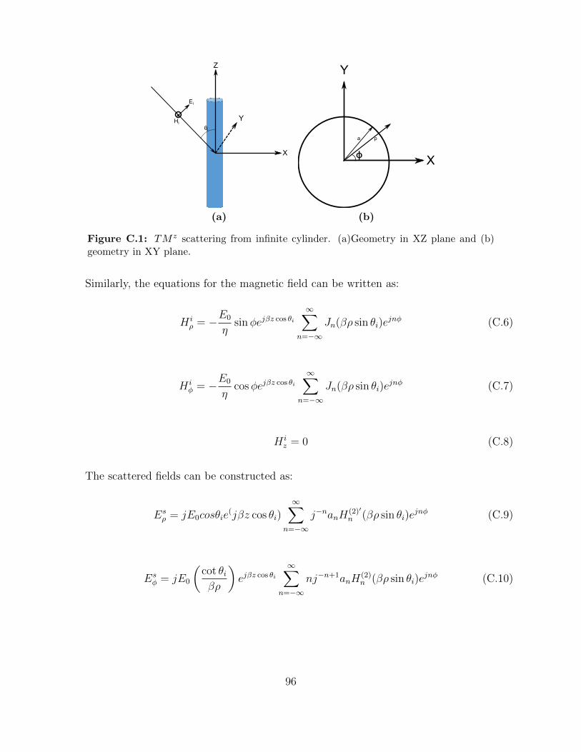
X

Z

θi

YHi

Ei

(a)

X

Y

ϕ

a ρ

(b)

Figure C.1: TM z scattering from infinite cylinder. (a)Geometry in XZ plane and (b)geometry in XY plane.

Similarly, the equations for the magnetic field can be written as:

H iρ = −E0

ηsinφejβz cos θi

∞∑n=−∞

Jn(βρ sin θi)ejnφ (C.6)

H iφ = −E0

ηcosφejβz cos θi

∞∑n=−∞

Jn(βρ sin θi)ejnφ (C.7)

H iz = 0 (C.8)

The scattered fields can be constructed as:

Esρ = jE0cosθie

(jβz cos θi)∞∑

n=−∞

j−nanH(2)′

n (βρ sin θi)ejnφ (C.9)

Esφ = jE0

(cot θiβρ

)ejβz cos θi

∞∑n=−∞

nj−n+1anH(2)n (βρ sin θi)e

jnφ (C.10)

96

Esz = E0 sin θie

jβzcosθi

∞∑n=−∞

j−nanH(2)n (βρ sin θi)e

jnφ (C.11)

Hsρ =

jE0

ωµρ sin θiejβzcosθi

∞∑n=−∞

nj−n+1anH(2)n (βρ sin θi)e

jnφ (C.12)

Hsφ = −jE0

ηe(jβz cos θi)

∞∑n=−∞

j−nanH(2)′

n (βρ sin θi)ejnφ (C.13)

where

an = − Jn(βa sin θi)

H(2)n (βa sin θi)

(C.14)

The total current induced on the surface can be computed as ~J = n× ( ~Hi+ ~Hs)∣∣∣ρ=a

This

results in

~J = −jE0

ηejβz cos θi

∞∑n=−∞

j−nJn(βa sin θi)

H(2)n

[cosφ

jH(2)n (βasinθi)−H(2)

n (βρ sin θi)

]ejnφ

(C.15)

Now, for cases where (a sin θi � λ), only the n = 0 term dominates. Using the small

argument values of the Hankel functions, the current can be approximated as:

H(2)′

0 (βa sin thetai) ≈ −j2

πβa sin θi(C.16)

H(2)0 (βa sin thetai) ≈ −j

2

πln (0.8905βa sin θi) (C.17)

97

Figure C.2: Variation of peak current induced on the cylinder for various angles asfunction of a/λ. Note that the currents begin to get singular as a sin θ → 0.

J ≈ jE0

ηejβz cos θi

1

aβ sin θi

1

ln(0.89aβ sin θi)(C.18)

The variation of peak currents as a function of radius can be seen is Fig. (C.2). A

significant observation here is that the current density tends to become singular as βa sin θi →

0. This can happen in two scenarios: The radius of the wires being much lesser than

the wavelength or the angle of incidence θi → 0. The latter case presents an interesting

phenomenon. It implies that as the angle of incidence θi increases, the effective radius of the

wire decreases, causing greater induced currents.

For mesh surfaces, it is only intuitive to expect that the openings also get scaled by sin θi,

and could be the reason for the reflection coefficients tending towards unity for very oblique

incidences, as predicted by the Astrakhan’s formulation.

98

APPENDIX D

Radiation from Uniformly Illuminated Elliptical

Apertures

Assume that an elliptical aperture is illuminated by a plane wave polarized in X direction,

with reference to Fig. D.1.

The incident wave equations can be written as:

~Ei = E0ejβzx (D.1)

~Hi =E0

ηejβzy (D.2)

Assuming the aperture lies in z = 0 plane, the field on the disc can be written as:

~Ei = E0x (D.3)

~Hi =E0

ηy (D.4)

For reflector applications, the aperture dimensions are usually much greater than the

wavelength, making Physical Optics a valid approximation.

~Jpo = 2n× ~Hi (D.5)

99

Figure D.1: An elliptical aperture illuminated by a plane wave normally incident, linearlypolarized in X direction.

with n = z, (D.5) yields

~Jpo =2E0

ηx (D.6)

Using, (D.6), the magnetic vector potential can be written as

~A =µ

4π

e−jβr

r

∫∫s

~Jpoejβ~r′.rds (D.7)

where r′ denotes the coordinates of the radiating aperture and r denotes the far field obser-

vation direction.

~r′.r = (aρ′ cosφ′x+ bρ′ sinφ′y).(sin θ cosφx+ sinθ sinφy) (D.8)

100

Which simplifies to

~r′.r = aρ′ cosφ′ sin θ cosφ+ bρ′ sinφ′ sin θ sinφ (D.9)

The x− directed current can be decomposed into its spherical components as:

Jθ = Jx.θ =2E0

ηcos θ cosφ (D.10)

Jφ = Jx.θ = −2E0

ηsinφ (D.11)

Substituting D.9, D.10 and D.11 in D.7 yields

Aθ =µ

4π

e−jβr

rNθ (D.12)

Aφ =µ

4π

e−jβr

rNφ (D.13)

Where,

Nθ =4πE0

ηcos θ cosφ

1

β√a2 sin2 θ cos2 φ+ b2 sin2 θ sin2 φ

J1(

√a2 sin2 θ cos2 φ+ b2 sin2 θ sin2 φ)

(D.14)

Nφ = −4πE0

ηsinφ

1

β√a2 sin2 θ cos2 φ+ b2 sin2 θ sin2 φ

J1(

√a2 sin2 θ cos2 φ+ b2 sin2 θ sin2 φ)

(D.15)

The far field electric fields can be constructed as:

Eθ = −jωAθ (D.16)

101

X

Z

Semi major axis (XZ plane)=1mSemi minor axis (YZ plane)=0.32mF/D (XZ plane)=5F/D (YZ plane)=15.62

10m

Figure D.2: A reflector antenna of large F/D to emulate plane wave normally incidenton an elliptical aperture.

Eφ = −jωAφ (D.17)

With Eθ and Eφ known, the copol and crosspol components can be constructed from

Ludwig’s 3rd definition [69] as:

Eco = cosφEθ − sinφEφ (D.18)

Ecross = sinφEθ + cosφEφ (D.19)

These expressions can be checked by simulating an elliptical aperture of a large F/D

ratio. The geometry is shown in Fig. D.2. The comparison of the analytical results with the

simulated results are shown in Fig. D.3.

102

−2 −1.5 −1 −0.5 0 0.5 1 1.5 2−80

−70

−60

−50

−40

−30

−20

−10

0

Theta (degrees)

Nor

mal

ized

Dire

ctiv

ity (

dBi)

copol(Elliptical aperture)copol (analytical)

(a)

−2 −1.5 −1 −0.5 0 0.5 1 1.5 2−80

−70

−60

−50

−40

−30

−20

−10

0

Theta (degrees)

Nor

mal

ized

Dire

ctiv

ity (

dBi)

copol (Elliptical aperture)copol (Analytical)

(b)

−2 −1.5 −1 −0.5 0 0.5 1 1.5 2−80

−70

−60

−50

−40

−30

−20

−10

0

Theta (degrees)

Nor

mal

ized

Dire

ctiv

ity (

dBi)

copol(Elliptical aperture)xpol(Elliptical aperture)copol (Analytical)xpol (Analytical)

(c)

Figure D.3: Comparison between the simulated results for a reflector antenna with anelliptical aperture of F/D = 5 in E-plane and F/D = 15.62 in H-plane with analyticalformulation. (a)E-plane. (b) H-plane. (c)D-plane.

103

References

[1] M. A. Swartwout, “CubeSat Database.” https://sites.google.com/a/slu.edu/

swartwout/home/cubesat-database. Accessed April 10, 2016.

[2] S. Lee et al., “CubeSat Design Specification,” The CubeSat Program, vol. 8651, p. 22,2009.

[3] ARC Mission Design Division Staff, “Small Spacecraft Technology State of the Art,”Tech. Rep. NASA/TP–2014–216648/REV1, NASA Ames Research Center, MoffetField, CA, 2014.

[4] M. Deshpande and J. Piepmeier, “Design and Development of VHF Antennas for SpaceBorne Signal of Opportunity Receivers for Cubesat Platforms,” 2015.

[5] T. Sato, R. Mitsuhashi, and S. Satori, “Attitude Estimation of Nano-Satellite HIT-SAT Using Received Power Fluctuation by Radiation Pattern,” in IEEE InternationalSymposium on Antennas and Propagation, 2009.

[6] R. Lehmensiek, “Using the physical structure of a passive aerodynamic attitude-stabilization system as a multi-frequency antenna on nano-satellites,” IEEE Antennasand Propagation Magazine, vol. 54, no. 3, pp. 39–49, 2012.

[7] T. J. Mizuno, J. D. Roque, B. T. Murakami, L. K. Yoneshige, G. S. Shiroma, R. Y.Miyamoto, and W. A. Shiroma, “Antennas for Distributed Nanosatellite Networks,” inIEEE/ACES International Conference on Wireless Communications and Applied Com-putational Electromagnetics, pp. 606–609, 2005.

[8] E. S. Moghaddam, N. Aboutorabian, S. Amiri, S. Nikmehr, and P. Rezaei, “Design andAnalysis of a Dualband Antenna for Small LEO Satellite Applications,” in InternationalConference on Computational Electromagnetics and Its Applications, pp. 228–231, 2004.

[9] M. Nohmi, K. Oi, S. Takuma, and M. Ogawa, “Solar Paddle Antenna Mounted onPico-Satellite” KUKAI” for Amateur Radio Communication,” in Second InternationalConference on Advances in Satellite and Space Communications, pp. 31–36, 2010.

[10] J. Costantine, Y. Tawk, A. Ernest, and C. Christodoulou, “Deployable Antennas forCubeSat and Space communications,” in 6th European Conference on Antennas andPropagation (EUCAP), pp. 837–840, 2012.

[11] P. Rezaei, “Design of Quadrifilar Helical Antenna for Use on Small Satellites,” in IEEEInternational Symposium on Antennas and Propagation, vol. 3, pp. 2895–2898, 2004.

[12] P. Muri, O. Challa, and J. McNair, “Enhancing Small Satellite Communication ThroughEffective Antenna System Design,” in Military Communications Conference (MIL-COM), pp. 347–352, 2010.

104

[13] G. Olson, S. Pellegrino, J. Costantine, and J. Banik, “Structural Architectures for a De-ployable Wideband UHF antenna,” in Structural Dynamics and Materials Conference,pp. 23–26, 2012.

[14] E. Pittella, S. Pisa, and A. Nascetti, “Design of an Antenna System for CubeSat Satel-lites,” in Proceedings of the 2nd IAA Conference on University Satellites Missions andCubeSat Winter Workshop, 2013.

[15] M. T. Islam, M. Cho, M. Samsuzzaman, and S. Kibria, “Compact Antenna for SmallSatellite Applications,” IEEE Antennas and Propagation Magazine, vol. 57, no. 2,pp. 30–36, 2015.

[16] F. E. Tubbal, R. Raad, and K.-W. Chin, “A Survey and Study of Planar Antennas forPico-Satellites,” IEEE Access, vol. 3, pp. 2590–2612, 2015.

[17] R. Montano, N. Neveu, S. Palacio, E. Martinez, D. R. Jackson, J. Chen, P. W. Fink,and R. S. Provence, “Development of low-profile antennas for cubesats,” 2014.

[18] A. Budianu, A. Meijerink, M. J. Bentum, D. M. Smith, and A.-J. Boonstra, “AntennaArchitecture of a Nano-Satellite for Radio Astronomy,” in IEEE Aerospace Conference,pp. 1–10, 2014.

[19] G. F. Kurnia, B. S. Nugroho, and A. D. Prasetyo, “Planar Inverted-F Antenna (PIFA)Array With Circular Polarization for Nano Satellite Application,” in International Sym-posium on Antennas and Propagation (ISAP), pp. 431–432, 2014.

[20] G. Dassano and M. Orefice, “The PICPOT Satellite Antenna Systems,” in IEEE Inter-national Symposium on Antennas and Propagation, pp. 3029–3032, 2007.

[21] J. Padilla, G. Rosati, A. Ivanov, F. Bongard, S. Vaccaro, and J. Mosig, “Multi-Functional Miniaturized Slot Antenna System for Small Satellites,” in European Con-ference on Antennas and Propagation, pp. 2170–2174, 2011.

[22] J. Klein, J. Hawkins, and D. Thorsen, “Improving CubeSat Downlink Capacity withActive Phased Array Antennas,” in IEEE Aerospace Conference, pp. 1–8, 2014.

[23] S. Tariq and R. Baktur, “Circularly Polarized UHF Up-and Downlink Antennas Inte-grated With CubeSat Solar Panels,” in IEEE International Symposium on Antennasand Propagation & USNC/URSI National Radio Science Meeting, pp. 1424–1425, 2015.

[24] R. M. Rodriguez-Osorio and E. F. Ramirez, “A Hands-On Education Project: AntennaDesign for Inter-CubeSat Communications,” IEEE Antennas and Propagation Maga-zine, vol. 54, no. 5, pp. 211–224, 2012.

105

[25] L. M. Hilliard, J. Mead, R. Rincon, and P. H. Hildebrand, “Lightweight Linear Broad-band Antennas Enabling Small UAV Wing Systems and Space Flight Nanosat Concept,”in IEEE International Geoscience and Remote Sensing Symposium, vol. 5, pp. 3577–3580, 2004.

[26] E. Palantei, S. Syarif, B. Topalaguna, and Z. Ubaid, “Four Elements Array of LungsShape Patch Antenna for Nanosatellite Telemetry,” in IEEE International Symposiumon Antennas and Propagation, pp. 1808–1809, 2013.

[27] O. Ceylan, Y. Kurt, F. A. Tunc, H. B. Yagci, and A. R. Aslan, “Low Cost S BandCommunication System Design for Nano Satellites,” in 5th International Conference onRecent Advances in Space Technologies, pp. 767–770, 2011.

[28] W. N. Saputra, B. Prasetya, and Y. Wahyu, “Design and Realization of two ArrayTriangle Patch of Microstrip Antenna with Gold Plate at Frequency 2400–2450 MHzfor Hexagonal Nanosatellite,” in International Conference of Information and Commu-nication Technology, pp. 322–327, 2013.

[29] C. A. Bergsrud and S. Noghanian, “Microstrip Aperture-Coupled Antenna Design forIn-Space Power Reception Experiment Using Nano-Sized Satellite,” in USNC-URSIRadio Science Meeting, pp. 25–25, 2015.

[30] J. Fouany, M. Thevenot, E. Arnaud, F. Torres, T. Monediere, N. Adnet, R. Manrique,L. Duchesne, J. Baracco, and K. Elis, “Circurlaly Polarized Isoflux Compact X BandAntenna for Nano-satellites Applications,” in European Radar Conference, pp. 381–384,2015.

[31] M. P. Magalhaes, M. V. Heckler, J. Mota, A. S. Sombra, and E. C. Moreira, “Designand Analysis of Microstrip Antenna Arrays for Meteorological Nano-Satellites for UHFUplink,” in International Telecommunications Symposium, pp. 1–5, 2014.

[32] M. K. Watanabe, R. N. Pang, B. O. Takase, J. M. Akagi, G. S. Shiroma, and W. A.Shiroma, “A 2-D Phase-Detecting/Heterodyne-Scanning Retrodirective Array,” IEEETransactions on Microwave Theory and Techniques, vol. 55, no. 12, pp. 2856–2864,2007.

[33] T. Sreeja, A. Arun, and J. Jaya Kumari, “An S-Band Micro-Strip Patch Array Antennafor Nano-Satellite Applications,” in International Conference on Green Technologies,pp. 325–328, 2012.

[34] E. Arnieri, L. Boccia, G. Amendola, and G. Di Massa, “A Compact High Gain Antennafor Small Satellite Applications,” IEEE Transactions on Antennas and Propagation,vol. 55, no. 2, pp. 277–282, 2007.

106

[35] B. T. Murakami, J. D. Roque, S. S. Sung, G. S. Shiroma, R. Y. Miyamoto, and W. A.Shiroma, “A Quadruple Subharmonic Phase-Conjugating Array for Secure Picosatel-lite Crosslinks,” in IEEE MTT-S International Microwave Symposium Digest, vol. 3,pp. 1687–1690, 2004.

[36] C. Hamrouni, A. Abraham, and A. Alimi, “Both Sides Linked Antenna Array for UltraSmall Satellite Communication Subsystem,” in International Conference on InnovationManagement and Technology Research, pp. 230–235, 2012.

[37] J. R. Saberin and C. Furse, “Challenges With Optically Transparent Patch Antennasfor Small Satellites,” in IEEE International Symposium on Antennas and Propagation,pp. 1–4, 2010.

[38] J. Li, S. Gao, and J. Xu, “Circularly Polarized High-gain Printed Antennas for SmallSatellite Applications,” in International Conference on Microwave Technology and Com-putational Electromagnetics, pp. 76–79, 2009.

[39] K. F. Warnick, “High Efficiency Phased Array Feed Antennas for Large Radio Tele-scopes and Small Satellite Communications Terminals,” in European Conference onAntennas and Propagation, pp. 448–449, 2013.

[40] F. E. Tubbal, R. Raad, K.-W. Chin, and B. Butters, “S-band Shorted Patch antennafor Inter Pico Satellite Communications,” in 8th International Conference on Telecom-munication Systems Services and Applications, pp. 1–4, 2014.

[41] P. R. Akbar, H. Saito, M. Zang, J. Hirokawa, and M. Ando, “X-band Parallel-Plate SlotArray Antenna for SAR Sensor Onboard 100 kg Small Satellite,” in IEEE InternationalSymposium on Antennas and Propagation, pp. 208–209, 2015.

[42] G. Codispoti, M. Lisi, and V. Santachiara, “X-band SAR Active Antenna Design forSmall Satellite Applications,” in IEEE International Symposium on Antennas and Prop-agation, vol. 1, pp. 666–669, 1995.

[43] Y. Yao, S. Liao, J. Wang, K. Xue, E. A. Balfour, and Y. Luo, “A New Patch AntennaDesigned for CubeSat: Dual feed, L/S dual-band stacked, and circularly polarized,”IEEE Antennas and Propagation Magazine, vol. 58, June 2016.

[44] S. Gunaseelan and M. Murugan, “High Gain Patch Antenna for CubeSat,” in Inter-national Conference on Wireless Communications, Signal Processing and Networking(WiSPNET), pp. 52–54, March 2016.

[45] M. Aherne, T. Barrett, L. Hoag, E. Teegarden, and R. Ramadas, “Aeneas–Colony IMeets Three-Axis Pointing,” 2011.

107

[46] A. Babuscia, M. Van de Loo, Q. J. Wei, S. Pan, S. Mohan, and S. Seager, “InflatableAntenna for CubeSat: Fabrication, Deployment and Results of Experimental Tests,” inIEEE Aerospace Conference, pp. 1–12, 2014.

[47] N. Chahat, J. Sauder, M. Thomson, R. Hodges, and Y. Rahmat-Samii, “CubeSat De-ployable Ka-Band Reflector Antenna for Deep Space missions,” in IEEE InternationalSymposium on Antennas and Propagation & USNC/URSI National Radio Science Meet-ing, pp. 2185–2186, 2015.

[48] V. Manohar and Y. Rahmat-Samii, “Characterization of Ka-Band Mesh Surfaces forCubeSat Reflector Antennas: From Simple Wire Grid Model to Complex Knits,” inURSI National Radio Science Meeting, pp. 1–2, 2016.

[49] R. Barrett, R. Taylor, P. Keller, D. Codell, and L. Adams, “Deployable Reflectors forSmall Satellites,” in Annual AIAA/USU Conference on Small Satellites, 2007.

[50] L. Periasamy and A. J. Gasiewski, “Precision Design, Analysis and Manufacturing ofQuasi-Optic Lens/Reflector Antenna Systems for CubeSat MMW/SMMW Radiome-ters,” in Radio Science Meeting (Joint with AP-S Symposium), pp. 265–265, 2015.

[51] M. Takikawa, Y. Inasawa, and Y. Konishi, “One-Dimensional Beam Scanning ReflectorAntenna for Small Satellite Applications,” in IEEE-APS Topical Conference on Anten-nas and Propagation in Wireless Communications, pp. 159–162, 2012.

[52] E. Peral et al., “RaInCube: A Proposed Constellation of Precipitation Profiling RadarsIn Cubesat,” in IEEE Symposium on International Geoscience and Remote Sensing,pp. 1261–1264, 2015.

[53] Y. Rahmat-Samii, “Reflector antennas,” in Antenna handbook (Y. Lo and S. Lee, eds.),ch. 15, New York: Van nostrand reinhold, 1993.

[54] P. G. Ingerson and W. C. Wong, “The Analysis of Deployable Umbrella ParabolicReflectors,” IEEE Transactions on Antennas and Propagation,, vol. 20, no. 4, pp. 409–414, 1972.

[55] F. L. Hai, “The Principle Error and Optimal Feed Point of Umbrella-Like ParabolicReflector,” in International Symposium on Antennas, Propagation and EM theory (IS-APE), pp. 697–700, 2000.

[56] J. Ruze, “Antenna Tolerance Theory - A Review,” Proceedings of the IEEE, vol. 54,pp. 633–640, April 1966.

[57] Y. Rahmat-Samii, “Effects of Deterministic Surface Distortions on Reflector AntennaPerformance,” in Annales des telecommunications, vol. 40, pp. 350–360, Springer, 1985.

108

[58] K. Bahadori and Y. Rahmat-Samii, “Characterization of Effects of Periodic and Ape-riodic Surface Distortions on Membrane Reflector Antennas,” IEEE Transactions onAntennas and Propagation, vol. 53, pp. 2782–2791, Sept 2005.

[59] K. Pontoppidan, “Reflector Antennas - An Overview of Surface Distortion Effects,” inProceedings JINA, pp. 82–93, 1986.

[60] M. Astrakhan, “Reflecting and Screening Properties of Plane Wire Grids,” Telecommu-nications and Radio Engineering-USSR, no. 1, p. 76, 1968.

[61] Y. Rahmat-Samii and S.-W. Lee, “Vector Diffraction Analysis of Reflector Antennaswith Mesh Surfaces,” IEEE Transactions on Antennas and Propagation, vol. 33, pp. 76– 90, jan 1985.

[62] A. Miura and Y. Rahmat-Samii, “Spaceborne Mesh Reflector Antennas With ComplexWeaves: Extended PO/Periodic-MoM Analysis,” IEEE Transactions on Antennas andPropagation, vol. 55, pp. 1022 –1029, april 2007.

[63] W. A. Imbriale, V. Galindo-Israel, and Y. Rahmat-Samii, “On the Reflectivity of Com-plex Mesh Surfaces,” IEEE Transactions on Antennas and Propagation, vol. 39, no. 9,pp. 1352–1365, 1991.

[64] D. Hill and J. Wait, “Analyses of Electromagnetic Scattering from Wire-Mesh Struc-tures,” Electronics Letters, vol. 12, no. 17, pp. 427–428, 1976.

[65] D. Hill and J. Wait, “Electromagnetic Scattering of an Arbitrary Plane Wave by a WireMesh with Bonded Junctions,” Canadian Journal of Physics, vol. 54, no. 4, pp. 353–361,1976.

[66] D. Hill and J. Wait, “Electromagnetic Scattering of an Arbitrary Plane Wave by TwoNonintersecting Perpendicular Wire Grids,” Canadian Journal of Physics, vol. 52, no. 3,pp. 227–237, 1974.

[67] T. Larsen, “A Survey of the Theory of Wire Grids,” IRE Transactions on MicrowaveTheory and Techniques, vol. 10, no. 3, pp. 191–201, 1962.

[68] H. Rajagopalan, A. Miura, and Y. Rahmat-Samii, “Equivalent Strip Width for Cylindri-cal Wire for Mesh Reflector Antennas: Experiments, Waveguide, and Plane-Wave Sim-ulations,” IEEE Transactions on Antennas and Propagation, vol. 54, no. 10, pp. 2845–2853, 2006.

[69] A. Ludwig, “The Definition of Cross Polarization,” IEEE Transactions on Antennasand Propagation, vol. 21, pp. 116–119, Jan 1973.

[70] C. A. Balanis, “Antenna Theory: Analysis and Design,” 2016.

109

[71] K. S. Rao and L. Shafai, “Phase Center Calculations of Reflector Antenna Feeds,” IEEEtransactions on antennas and propagation, vol. 32, pp. 740–742, 1984.

[72] E. I. Muehldorf, “The Phase Center of Horn Antennas,” IEEE Transactions on Anten-nas and Propagation, vol. 18, no. 6, pp. 753–760, 1970.

[73] Y. Hu, “A Method of Determining Phase Centers and its Application to ElectromagneticHorns,” Journal of the Franklin Institute, vol. 271, no. 1, pp. 31–39, 1961.

110