Using Python for Interactive Data Analysis

Perry GreenfieldRobert Jedrzejewski

Space Telescope Science Institute

June 13, 2005

1

Copyright (c) 2005, Association of Universities for Research in Astronomy, Inc (AURA). Allrights reserved.

2

ContentsPurpose 7

Prerequisites 7

Practicalities 7

1 Reading and manipulating image data 81.1 Example session to read and display an image from a FITS file . . . . . . . . . . . . . . . . . 81.2 Starting the Python interpreter . . . . . . . . . . . . . . . . . . . . . . . . . . . . . . . . . . . 81.3 Loading modules . . . . . . . . . . . . . . . . . . . . . . . . . . . . . . . . . . . . . . . . . . . 81.4 Reading data from FITS files . . . . . . . . . . . . . . . . . . . . . . . . . . . . . . . . . . . . 91.5 Displaying images . . . . . . . . . . . . . . . . . . . . . . . . . . . . . . . . . . . . . . . . . . 91.6 Array expressions . . . . . . . . . . . . . . . . . . . . . . . . . . . . . . . . . . . . . . . . . . . 91.7 FITS headers . . . . . . . . . . . . . . . . . . . . . . . . . . . . . . . . . . . . . . . . . . . . . 101.8 Writing data to FITS files . . . . . . . . . . . . . . . . . . . . . . . . . . . . . . . . . . . . . . 101.9 Some Python basics . . . . . . . . . . . . . . . . . . . . . . . . . . . . . . . . . . . . . . . . . 11

1.9.1 Memory vs. data files . . . . . . . . . . . . . . . . . . . . . . . . . . . . . . . . . . . . 111.9.2 Python variables . . . . . . . . . . . . . . . . . . . . . . . . . . . . . . . . . . . . . . . 111.9.3 How does object oriented programming affect you? . . . . . . . . . . . . . . . . . . . . 111.9.4 Errors and dealing with them . . . . . . . . . . . . . . . . . . . . . . . . . . . . . . . . 12

1.10 Array basics . . . . . . . . . . . . . . . . . . . . . . . . . . . . . . . . . . . . . . . . . . . . . . 131.10.1 Creating arrays . . . . . . . . . . . . . . . . . . . . . . . . . . . . . . . . . . . . . . . . 131.10.2 Array numeric types . . . . . . . . . . . . . . . . . . . . . . . . . . . . . . . . . . . . . 141.10.3 Printing arrays . . . . . . . . . . . . . . . . . . . . . . . . . . . . . . . . . . . . . . . . 141.10.4 Indexing 1-D arrays . . . . . . . . . . . . . . . . . . . . . . . . . . . . . . . . . . . . . 151.10.5 Indexing multidimensional arrays . . . . . . . . . . . . . . . . . . . . . . . . . . . . . . 161.10.6 Compatibility of dimensions . . . . . . . . . . . . . . . . . . . . . . . . . . . . . . . . . 161.10.7 ufuncs . . . . . . . . . . . . . . . . . . . . . . . . . . . . . . . . . . . . . . . . . . . . . 171.10.8 Array functions . . . . . . . . . . . . . . . . . . . . . . . . . . . . . . . . . . . . . . . . 181.10.9 Array methods . . . . . . . . . . . . . . . . . . . . . . . . . . . . . . . . . . . . . . . . 201.10.10Array attributes: . . . . . . . . . . . . . . . . . . . . . . . . . . . . . . . . . . . . . . . 21

1.11 Example . . . . . . . . . . . . . . . . . . . . . . . . . . . . . . . . . . . . . . . . . . . . . . . . 211.12 Exercises . . . . . . . . . . . . . . . . . . . . . . . . . . . . . . . . . . . . . . . . . . . . . . . 21

2 Reading and plotting spectral data 232.1 Example session to read spectrum and plot it . . . . . . . . . . . . . . . . . . . . . . . . . . . 232.2 An aside on how Python finds modules . . . . . . . . . . . . . . . . . . . . . . . . . . . . . . . 232.3 Reading FITS table data . . . . . . . . . . . . . . . . . . . . . . . . . . . . . . . . . . . . . . . 242.4 Quick introduction to plotting . . . . . . . . . . . . . . . . . . . . . . . . . . . . . . . . . . . . 25

2.4.1 Simple x-y plots . . . . . . . . . . . . . . . . . . . . . . . . . . . . . . . . . . . . . . . 252.4.2 Labeling plot axes . . . . . . . . . . . . . . . . . . . . . . . . . . . . . . . . . . . . . . 262.4.3 Overplotting . . . . . . . . . . . . . . . . . . . . . . . . . . . . . . . . . . . . . . . . . 272.4.4 Legends and annotation . . . . . . . . . . . . . . . . . . . . . . . . . . . . . . . . . . . 282.4.5 Saving and printing plots . . . . . . . . . . . . . . . . . . . . . . . . . . . . . . . . . . 28

2.5 A little background on Python sequences . . . . . . . . . . . . . . . . . . . . . . . . . . . . . 292.5.1 Strings . . . . . . . . . . . . . . . . . . . . . . . . . . . . . . . . . . . . . . . . . . . . . 292.5.2 Lists . . . . . . . . . . . . . . . . . . . . . . . . . . . . . . . . . . . . . . . . . . . . . . 312.5.3 Tuples . . . . . . . . . . . . . . . . . . . . . . . . . . . . . . . . . . . . . . . . . . . . . 312.5.4 Standard operations on sequences . . . . . . . . . . . . . . . . . . . . . . . . . . . . . 322.5.5 Dictionaries . . . . . . . . . . . . . . . . . . . . . . . . . . . . . . . . . . . . . . . . . . 322.5.6 A section about nothing . . . . . . . . . . . . . . . . . . . . . . . . . . . . . . . . . . . 34

2.6 More on plotting . . . . . . . . . . . . . . . . . . . . . . . . . . . . . . . . . . . . . . . . . . . 342.6.1 matplotlib terminology, configuration and modes of usage . . . . . . . . . . . . . . . 34

3

2.6.2 matplot functions . . . . . . . . . . . . . . . . . . . . . . . . . . . . . . . . . . . . . . . 352.7 Plotting mini-Cookbook . . . . . . . . . . . . . . . . . . . . . . . . . . . . . . . . . . . . . . . 36

2.7.1 customizing standard plots . . . . . . . . . . . . . . . . . . . . . . . . . . . . . . . . . 362.7.2 implot example . . . . . . . . . . . . . . . . . . . . . . . . . . . . . . . . . . . . . . . . 382.7.3 imshow example . . . . . . . . . . . . . . . . . . . . . . . . . . . . . . . . . . . . . . . 392.7.4 figimage . . . . . . . . . . . . . . . . . . . . . . . . . . . . . . . . . . . . . . . . . . . . 402.7.5 histogram example . . . . . . . . . . . . . . . . . . . . . . . . . . . . . . . . . . . . . . 402.7.6 contour example . . . . . . . . . . . . . . . . . . . . . . . . . . . . . . . . . . . . . . . 412.7.7 subplot example . . . . . . . . . . . . . . . . . . . . . . . . . . . . . . . . . . . . . . . 422.7.8 readcursor example . . . . . . . . . . . . . . . . . . . . . . . . . . . . . . . . . . . . . . 43

2.8 Exercises . . . . . . . . . . . . . . . . . . . . . . . . . . . . . . . . . . . . . . . . . . . . . . . 44

3 More advanced topics in PyFITS, numarray and IPython 453.1 IPython . . . . . . . . . . . . . . . . . . . . . . . . . . . . . . . . . . . . . . . . . . . . . . . . 45

3.1.1 Obtaining information about Python objects and functions . . . . . . . . . . . . . . . 453.1.2 Access to the OS shell . . . . . . . . . . . . . . . . . . . . . . . . . . . . . . . . . . . . 463.1.3 Magic commands . . . . . . . . . . . . . . . . . . . . . . . . . . . . . . . . . . . . . . . 473.1.4 Syntax shortcuts . . . . . . . . . . . . . . . . . . . . . . . . . . . . . . . . . . . . . . . 483.1.5 IPython history features . . . . . . . . . . . . . . . . . . . . . . . . . . . . . . . . . . . 49

3.2 Python Introspection . . . . . . . . . . . . . . . . . . . . . . . . . . . . . . . . . . . . . . . . . 493.3 Saving your data . . . . . . . . . . . . . . . . . . . . . . . . . . . . . . . . . . . . . . . . . . . 503.4 Python loops and conditionals . . . . . . . . . . . . . . . . . . . . . . . . . . . . . . . . . . . . 50

3.4.1 The for statement . . . . . . . . . . . . . . . . . . . . . . . . . . . . . . . . . . . . . . 503.4.2 Blocks of code, and indentation . . . . . . . . . . . . . . . . . . . . . . . . . . . . . . . 513.4.3 Python if statements . . . . . . . . . . . . . . . . . . . . . . . . . . . . . . . . . . . . . 513.4.4 What’s True and what’s False . . . . . . . . . . . . . . . . . . . . . . . . . . . . . . . . 523.4.5 The in crowd . . . . . . . . . . . . . . . . . . . . . . . . . . . . . . . . . . . . . . . . . 52

3.5 Advanced PyFITS Topics . . . . . . . . . . . . . . . . . . . . . . . . . . . . . . . . . . . . . . 523.5.1 Header manipulations . . . . . . . . . . . . . . . . . . . . . . . . . . . . . . . . . . . . 523.5.2 PyFITS Object Oriented Interface . . . . . . . . . . . . . . . . . . . . . . . . . . . . . 533.5.3 Controlling memory usage . . . . . . . . . . . . . . . . . . . . . . . . . . . . . . . . . . 533.5.4 Support for common FITS conventions . . . . . . . . . . . . . . . . . . . . . . . . . . . 543.5.5 Noncompliant FITS data . . . . . . . . . . . . . . . . . . . . . . . . . . . . . . . . . . 54

3.6 A quick tour of standard numarray packages . . . . . . . . . . . . . . . . . . . . . . . . . . . . 553.6.1 random_array . . . . . . . . . . . . . . . . . . . . . . . . . . . . . . . . . . . . . . . . 553.6.2 fft . . . . . . . . . . . . . . . . . . . . . . . . . . . . . . . . . . . . . . . . . . . . . . . 563.6.3 convolve . . . . . . . . . . . . . . . . . . . . . . . . . . . . . . . . . . . . . . . . . . . . 573.6.4 linear_algebra . . . . . . . . . . . . . . . . . . . . . . . . . . . . . . . . . . . . . . . . 573.6.5 MA (Masked Arrays) . . . . . . . . . . . . . . . . . . . . . . . . . . . . . . . . . . . . 573.6.6 nd_image (Multi-dimensional array processing) . . . . . . . . . . . . . . . . . . . . . . 583.6.7 ieespecial . . . . . . . . . . . . . . . . . . . . . . . . . . . . . . . . . . . . . . . . . . . 58

3.7 Intermediate numarray topics . . . . . . . . . . . . . . . . . . . . . . . . . . . . . . . . . . . . 583.7.1 The Zen of array programming . . . . . . . . . . . . . . . . . . . . . . . . . . . . . . . 583.7.2 The power of mask arrays, index arrays, and where() . . . . . . . . . . . . . . . . . . . 593.7.3 1-D polynomial interpolation example . . . . . . . . . . . . . . . . . . . . . . . . . . . 603.7.4 Radial profile example . . . . . . . . . . . . . . . . . . . . . . . . . . . . . . . . . . . . 603.7.5 Random ensemble simulation example . . . . . . . . . . . . . . . . . . . . . . . . . . . 613.7.6 thermal diffusion solution example . . . . . . . . . . . . . . . . . . . . . . . . . . . . . 623.7.7 Finding nearest neighbors . . . . . . . . . . . . . . . . . . . . . . . . . . . . . . . . . . 633.7.8 Cosmic ray detection in single image . . . . . . . . . . . . . . . . . . . . . . . . . . . . 633.7.9 Source extraction . . . . . . . . . . . . . . . . . . . . . . . . . . . . . . . . . . . . . . . 633.7.10 Other issues regarding efficiency and performance . . . . . . . . . . . . . . . . . . . . . 643.7.11 Customizing numeric error handling . . . . . . . . . . . . . . . . . . . . . . . . . . . . 64

4

4 Programming in Python 664.1 Introduction . . . . . . . . . . . . . . . . . . . . . . . . . . . . . . . . . . . . . . . . . . . . . . 66

4.1.1 Namespaces . . . . . . . . . . . . . . . . . . . . . . . . . . . . . . . . . . . . . . . . . . 664.2 Functions . . . . . . . . . . . . . . . . . . . . . . . . . . . . . . . . . . . . . . . . . . . . . . . 68

4.2.1 The basics . . . . . . . . . . . . . . . . . . . . . . . . . . . . . . . . . . . . . . . . . . . 684.2.2 Function argument handling . . . . . . . . . . . . . . . . . . . . . . . . . . . . . . . . . 69

4.3 Python scripts . . . . . . . . . . . . . . . . . . . . . . . . . . . . . . . . . . . . . . . . . . . . 714.4 Modules . . . . . . . . . . . . . . . . . . . . . . . . . . . . . . . . . . . . . . . . . . . . . . . . 724.5 Exception handling . . . . . . . . . . . . . . . . . . . . . . . . . . . . . . . . . . . . . . . . . . 744.6 Garbage (cleaning up after yourself) . . . . . . . . . . . . . . . . . . . . . . . . . . . . . . . . 754.7 Miscellany: . . . . . . . . . . . . . . . . . . . . . . . . . . . . . . . . . . . . . . . . . . . . . . 76

4.7.1 Interactive programs . . . . . . . . . . . . . . . . . . . . . . . . . . . . . . . . . . . . . 764.7.2 Text Handling . . . . . . . . . . . . . . . . . . . . . . . . . . . . . . . . . . . . . . . . 774.7.3 String formatting . . . . . . . . . . . . . . . . . . . . . . . . . . . . . . . . . . . . . . . 774.7.4 More about print . . . . . . . . . . . . . . . . . . . . . . . . . . . . . . . . . . . . . . 794.7.5 Line continuations . . . . . . . . . . . . . . . . . . . . . . . . . . . . . . . . . . . . . . 794.7.6 Variable name conventions . . . . . . . . . . . . . . . . . . . . . . . . . . . . . . . . . 794.7.7 Division . . . . . . . . . . . . . . . . . . . . . . . . . . . . . . . . . . . . . . . . . . . . 794.7.8 Implicit tuples and tuple assignment . . . . . . . . . . . . . . . . . . . . . . . . . . . . 804.7.9 What if your function needs to return more than one value? . . . . . . . . . . . . . . . 804.7.10 Equality versus identity . . . . . . . . . . . . . . . . . . . . . . . . . . . . . . . . . . . 80

4.8 Python module overview . . . . . . . . . . . . . . . . . . . . . . . . . . . . . . . . . . . . . . . 814.9 Debugging . . . . . . . . . . . . . . . . . . . . . . . . . . . . . . . . . . . . . . . . . . . . . . . 814.10 PyRAF . . . . . . . . . . . . . . . . . . . . . . . . . . . . . . . . . . . . . . . . . . . . . . . . 83

4.10.1 Basic features . . . . . . . . . . . . . . . . . . . . . . . . . . . . . . . . . . . . . . . . . 834.10.2 Using PyRAF . . . . . . . . . . . . . . . . . . . . . . . . . . . . . . . . . . . . . . . . . 844.10.3 Giving Python functions an IRAF personality . . . . . . . . . . . . . . . . . . . . . . . 85

4.11 Final thoughts . . . . . . . . . . . . . . . . . . . . . . . . . . . . . . . . . . . . . . . . . . . . 86

5 What is this object-oriented stuff anyway? 875.1 Class basics . . . . . . . . . . . . . . . . . . . . . . . . . . . . . . . . . . . . . . . . . . . . . . 87

5.1.1 Class definitions . . . . . . . . . . . . . . . . . . . . . . . . . . . . . . . . . . . . . . . 875.1.2 Python isn’t like other object oriented languages . . . . . . . . . . . . . . . . . . . . . 885.1.3 Classes as a generalized data structure . . . . . . . . . . . . . . . . . . . . . . . . . . . 885.1.4 Those ’magic’ methods . . . . . . . . . . . . . . . . . . . . . . . . . . . . . . . . . . . . 895.1.5 How classes get rich . . . . . . . . . . . . . . . . . . . . . . . . . . . . . . . . . . . . . 92

5.2 A more complex example: Representing Source Spectra . . . . . . . . . . . . . . . . . . . . . 935.2.1 Goals . . . . . . . . . . . . . . . . . . . . . . . . . . . . . . . . . . . . . . . . . . . . . 935.2.2 Initial Implementation . . . . . . . . . . . . . . . . . . . . . . . . . . . . . . . . . . . . 935.2.3 Basic object creation . . . . . . . . . . . . . . . . . . . . . . . . . . . . . . . . . . . . . 955.2.4 Spectrum addition . . . . . . . . . . . . . . . . . . . . . . . . . . . . . . . . . . . . . . 955.2.5 Evaluation of the spectrum at given wavelengths . . . . . . . . . . . . . . . . . . . . . 955.2.6 Why this is better than the traditional approach . . . . . . . . . . . . . . . . . . . . . 955.2.7 Take 2: handling multiplicative effects . . . . . . . . . . . . . . . . . . . . . . . . . . . 96

5.3 Further enhancements to the spectrum model . . . . . . . . . . . . . . . . . . . . . . . . . . . 1005.3.1 Determining total flux . . . . . . . . . . . . . . . . . . . . . . . . . . . . . . . . . . . . 1005.3.2 Handling empirical spectra . . . . . . . . . . . . . . . . . . . . . . . . . . . . . . . . . 1005.3.3 Valid wavelength ranges . . . . . . . . . . . . . . . . . . . . . . . . . . . . . . . . . . . 1015.3.4 Component normalization . . . . . . . . . . . . . . . . . . . . . . . . . . . . . . . . . . 1015.3.5 Redshifts . . . . . . . . . . . . . . . . . . . . . . . . . . . . . . . . . . . . . . . . . . . 1015.3.6 Different unit systems . . . . . . . . . . . . . . . . . . . . . . . . . . . . . . . . . . . . 102

5.4 The upside to object-oriented programs . . . . . . . . . . . . . . . . . . . . . . . . . . . . . . 1035.5 The downside . . . . . . . . . . . . . . . . . . . . . . . . . . . . . . . . . . . . . . . . . . . . . 1045.6 Loose ends . . . . . . . . . . . . . . . . . . . . . . . . . . . . . . . . . . . . . . . . . . . . . . 104

5

5.6.1 Method inheritance and overloading . . . . . . . . . . . . . . . . . . . . . . . . . . . . 1045.6.2 Object initialization . . . . . . . . . . . . . . . . . . . . . . . . . . . . . . . . . . . . . 1045.6.3 Multiple inheritance . . . . . . . . . . . . . . . . . . . . . . . . . . . . . . . . . . . . . 1055.6.4 New-style vs old-style classes . . . . . . . . . . . . . . . . . . . . . . . . . . . . . . . . 1055.6.5 Duck typing . . . . . . . . . . . . . . . . . . . . . . . . . . . . . . . . . . . . . . . . . . 105

5.7 What you haven’t learned about Python (so if you are interested, go look it up) . . . . . . . . 1055.7.1 iterators . . . . . . . . . . . . . . . . . . . . . . . . . . . . . . . . . . . . . . . . . . . . 1055.7.2 generators . . . . . . . . . . . . . . . . . . . . . . . . . . . . . . . . . . . . . . . . . . . 1055.7.3 list comprehensions . . . . . . . . . . . . . . . . . . . . . . . . . . . . . . . . . . . . . . 1065.7.4 sets . . . . . . . . . . . . . . . . . . . . . . . . . . . . . . . . . . . . . . . . . . . . . . 1065.7.5 metaclasses . . . . . . . . . . . . . . . . . . . . . . . . . . . . . . . . . . . . . . . . . . 106

5.8 The Zen of Python . . . . . . . . . . . . . . . . . . . . . . . . . . . . . . . . . . . . . . . . . . 106

6 Interfacing C & C++ programs 1086.1 Overview of different tools . . . . . . . . . . . . . . . . . . . . . . . . . . . . . . . . . . . . . . 108

6.1.1 Summary . . . . . . . . . . . . . . . . . . . . . . . . . . . . . . . . . . . . . . . . . . . 1096.2 Overview of manual interfacing . . . . . . . . . . . . . . . . . . . . . . . . . . . . . . . . . . . 1096.3 A few basic concepts before getting started . . . . . . . . . . . . . . . . . . . . . . . . . . . . 109

6.3.1 How Python finds and uses C extensions . . . . . . . . . . . . . . . . . . . . . . . . . . 1096.3.2 Compiling and Linking C Extensions . . . . . . . . . . . . . . . . . . . . . . . . . . . 1106.3.3 A Simple Example . . . . . . . . . . . . . . . . . . . . . . . . . . . . . . . . . . . . . . 1106.3.4 So what about more complicated examples? . . . . . . . . . . . . . . . . . . . . . . . . 1116.3.5 But what about using arrays? . . . . . . . . . . . . . . . . . . . . . . . . . . . . . . . . 111

6.4 General Pointers . . . . . . . . . . . . . . . . . . . . . . . . . . . . . . . . . . . . . . . . . . . 1116.4.1 Handling Calling Arguments . . . . . . . . . . . . . . . . . . . . . . . . . . . . . . . . 1126.4.2 Returning None . . . . . . . . . . . . . . . . . . . . . . . . . . . . . . . . . . . . . . . . 1126.4.3 Exceptions . . . . . . . . . . . . . . . . . . . . . . . . . . . . . . . . . . . . . . . . . . 1126.4.4 Reference Counting . . . . . . . . . . . . . . . . . . . . . . . . . . . . . . . . . . . . . 1136.4.5 Using debuggers on Python C Extensions . . . . . . . . . . . . . . . . . . . . . . . . . 1146.4.6 How to Make Your Module Schizophrenic . . . . . . . . . . . . . . . . . . . . . . . . . 114

6.5 A More Complex Example . . . . . . . . . . . . . . . . . . . . . . . . . . . . . . . . . . . . . 1146.6 numarray example . . . . . . . . . . . . . . . . . . . . . . . . . . . . . . . . . . . . . . . . . . 117

Acknowledgements 120

Appendix A: Python Books, Tutorials, and On-line Resources 121

Appendix B: Why would I switch from IDL to Python (or not)? 122

Appendix C: IDL/numarray feature mapping 125

Appendix D: matplotlib for IDL Users 128

Appendix E: Editors and Integrated Development Environments 135

Appendix F: Numeric vs numarray vs scipy vs Numeric3... 136

6

PurposeThis is intended to show how Python can be used to interactively analyze astronomical data much in thesame way IDL can. The approach taken is to illustrate as quickly as possible how one can perform commondata analysis tasks. This is not a tutorial on how to program in Python (many good tutorials are available—targeting various levels of programming experience—, either as books or on-line material; many are free).As with IDL, one can write programs and applications also rather than just execute interactive commands.(Appendix A lists useful books, tutorials and on-line resources for learning the Python language itself as wellas the specific modules addressed here.) Nevertheless, the focus will initially be almost entirely on interactiveuse. Later, as use becomes more sophisticated, more attention will be given to elements that are useful inwriting scripts or applications (which themselves may be used as interactive commands).

This document is not intended as a reference, but it is unconventional in that it does serve as a lightreference in that in many sections lists of functions or methods are given. The reasons are twofold: first,to give a quick overview of what capabilities are available. Generally these tables are limited to one linedescriptions; generally enough to give a good idea of what can be done, but not necessarily enough informationto use it (though often it is). Secondly, since the brief descriptions often sufficient to use the functions withoutresort to more detailed documentation, thus reducing the need to continually refer to other documentationif the user is using this document as a primary tool for learning how to use Python.

For those with IDL experience, Appendix B compares Python and IDL to aid those trying to decidewhether they should use Python; and Appendix C provides a mapping between IDL and Python arraycapabilities to help IDL users find corresponding ways to carry out the same actions. Appendix D comparesIDL plotting with matplotlib. Appendix E has some brief comments about editors and IDEs (IntegratedDevelopment Environments). Appendix F discusses the current situation regarding the two different arraypackages within Python.

PrerequisitesPrevious experience with Python of course is helpful, but is not assumed. Likewise, previous experience inusing an array manipulation language such as IDL or matlab is helpful, but not required. Some familiaritywith programming of some sort is necessary.

PracticalitiesThis tutorial series assumes that Python (v2.3 or later), numarray (v1.2.3 or later), matplotlib (v0.73.1 orlater), pyfits (v0.98 or later), numdisplay (v1.0 or later), and ipython (v0.6.12 or later) are installed (Googleto find the downloads if not already installed). All these modules will run on all standard Unix, Linux, MacOS X and MS Windows platforms (PyRAF is not supported on MS Windows since IRAF does not run onthat platform). The initial image display examples assume that DS9 (or ximtool) is installed.

At STScI these are all available on Science cluster machines and the following describes how to set upyour environment to access Python and these modules.

For the moment the PyFITS functions are available only on IRAFDEV. To make this version availableeither place IRAFDEV in your .envrc file or type irafdev at the shell level. Eventually this will be availablefor IRAFX as well.

If you have a Mac, and do not have all these items installed, follow the instructions on this web page:http://pyraf.stsci.edu/pyssg/macosx.html. At the very least you will need to do an update to get the latestPyFITS.

7

1 Reading and manipulating image data

1.1 Example session to read and display an image from a FITS fileThe following illustrates how one can get data from a simple FITS file and display the data to DS9 or similarimage display program. It presumes one has already started the image display program before startingPython. A short example of an interactive Python session is shown below (just the input commands, notwhat is printed out in return). The individual steps will be explained in detail in following sections.

> > > import pyfits # load FITS module> > > from numarray import * # load array module> > > pyfits.info(’pix.fits’) # show info about file> > > im = pyfits.getdata(’pix.fits’) # read image data from file> > > import numdisplay # load image display module> > > numdisplay.display(im) # display to DS9> > > numdisplay.display(im,z1=0,z2=300) # repeat with new cuts> > > fim = 1.*im # make float array> > > bigvals = where(fim > 10) # find pixels above threshold

# log scale above threshold> > > fim[bigvals] = 10*log(fim[bigvals]-10) + 10> > > numdisplay.display(fim)> > > hdr = pyfits.getheader(’pix.fits’)> > > print hdr> > > date = hdr[’date’] # print header keyword value> > > hdr[’date’] = ’4th of July’ # modify value> > > hdr.update(’flatfile’,’flat17.fits’) # add new keyword flatfile> > > pyfits.writeto(’newfile.fits’,fim,hdr) # create new fits file> > > pyfits.append(’existingfile.fits’,fim, hdr)> > > pyfits.update(’existingfile.fits’,fim, hdr, ext=3)

1.2 Starting the Python interpreterThe first step is to start the Python interpreter. There are several variants one can use. The plain Pythoninterpreter is standard with every Python installation, but lacks many features that you will find in PyRAFor IPython. We recommend that you use one of those as an interactive environment (ultimately PyRAFwill use IPython itself). For basic use they all pretty much do the same thing. IPython special featureswill be covered later. The examples will show all typed lines starting the line with the standard promptof the Python interpreter (> > >) unless it is IPython (numbered prompt) or PyRAF (prompt: -->) beingdiscussed. (Note that comments begin with #.) At the shell command line you type one of the following

python # starts standard Python interpreteripython # starts ipython (enhanced interactive features)pyraf # starts PyRAF

1.3 Loading modulesAfter starting an interpreter, we need to load the necessary libraries. One can do this explicitly, as in thisexample, or do it within a start-up file. For now we’ll do it explicitly. There is more than one way to load alibrary; each has its advantages. The first is the most common found in scripts:

> > > import pyfits

This loads the FITS I/O module. When modules or packages are loaded this way, all the items they contain(functions, variables, etc.) are in the “namespace” of the module and to use or access them, one must prefacethe item with the module name and a period, e.g., pyfits.getdata() to call the pyfits module getdatafunction.

8

For convenience, particularly in interactive sessions, it is possible to import the module’s contents directlyinto the working namespace so prefacing the functions with the name of the module is not necessary. Thefollowing shows how to import the array module directly into the namespace:

> > > from numarray import *

There are other variants on importing that will be mentioned later.

1.4 Reading data from FITS filesOne can see what a FITS file contains by typing:

> > > pyfits.info(’pix.fits’)Filename: pix.fitsNo. Name Type Cards Dimensions Format0 PRIMARY PrimaryHDU 71 (512, 512) Int16

The simplest way to access FITS files is to use the function getdata.

> > > im = pyfits.getdata(’pix.fits’)

If the fits file contains multiple extensions, this function will default to reading the data part of the primaryHeader Data Unit, if it has data, and if not, the data from the first extension. What is returned is, in thiscase, an image array (how tables are handled will be described in the next tutorial).

1.5 Displaying imagesMuch like IDL and Matlab, many things can be done with the array. For example, it is easy to find outinformation about the array: im.shape tells you about the dimensions of this array. The image can bedisplayed on a standard image display program such as DS9 (ximtool and SAOIMAGE will work too, solong as an 8-bit display is supported) using numdisplay (the following examples presume that the imagedisplay program has already been started):

> > > import numdisplay> > > numdisplay.display(im)

As one would expect, one can adjust the image cuts:

> > > numdisplay.display(im,z1=0,z2=300)

Note that Python functions accept both positional style arguments or keyword arguments.There are other ways to display images that will be covered in subsequent tutorials.

1.6 Array expressionsThe next operations show that applying simple operations to the whole or part of arrays is possible.

> > > fim = im*1.

creates a floating point version of the image.

> > > bigvals = where(fim > 10)

returns arrays indicating where in the fim array the values are larger than 10 (exactly what is being returnedis glossed over for the moment). This information can be used to index the corresponding values in the arrayto use only those values for manipulation or modification as the following expression does:

> > > fim[bigvals] = 10*log(fim[bigvals]-10) + 10

This replaces all of the values that are larger than 10 in the array with a scaled log value added to 10

> > > numdisplay.display(fim)

The details on how to manipulate arrays will be the primary focus of this tutorial.

9

1.7 FITS headersLooking at information in the FITS header is easy. To get the header one can use pyfits.getheader:

> > > hdr = pyfits.getheader(’pix.fits’)

Both header and data can be obtained at the same time using getdata with an optional header keywordargument (the ability to assign to two variables at once will be explained a bit more in a later tutorial; it’sparticularly useful when functions return more than one thing):

> > > data, hdr = pyfits.getdata(’pix.fits’, header=True)

To print out the whole header:

> > > print hdrSIMPLE = T / Fits standardBITPIX = 16 / Bits per pixelNAXIS = 2 / Number of axesNAXIS1 = 512 / Axis lengthNAXIS2 = 512 / Axis lengthEXTEND = F / File may contain extensions

[...]

CCDPROC = ’Apr 22 14:11 CCD processing done’AIRMASS = 1.08015632629395 / AIRMASSHISTORY ’KPNO-IRAF’HISTORY ’24-04-87’HISTORY ’KPNO-IRAF’ /HISTORY ’08-04-92’ /

To get the value of a particular keyword:

> > > date = hdr[’date’]> > > date’2004-06-05T15:33:51’

To change an existing keyword:

> > > hdr[’date’] = ’4th of July’

To change an existing keyword or add it if it doesn’t exist:

> > > hdr.update(’flatfile’,’flat17.fits’)

Where flatfile is the keyword name and flat17.fits is its value.Special methods are available to add history, comment or blank cards (see Tutorial 3 for examples).

When

1.8 Writing data to FITS files> > > pyfits.writeto(’newfile.fits’,fim,hdr) # User supplied header

or

> > > pyfits.append(’existingfile.fits’,fim, hdr)

or

> > > pyfits.update(’existingfile.fits’,fim, hdr, ext=3)

There are alternative ways of accessing FITS files that will be explained in a later tutorial that allow morecontrol over how files are written and updated.

10

1.9 Some Python basicsIt’s time to gain some understanding of what is going on when using Python tools to do data analysis thisway. Those familiar with IDL will see much similarity in the approach used. It may seem a bit more aliento those used to running programs or tasks in IRAF or similar systems.

1.9.1 Memory vs. data files

First it is important to understand that the results of what one does usually reside in memory rather thanin a data file. With IRAF, most tasks that process data produce a new or updated data file (if the result is asmall number of values it may appear in the printout or as a task parameter). In IDL or Python, one usuallymust explicitly write the results from memory to a data file. So results are volatile in the sense that they willbe lost if the session is ended. The advantage of doing things this way is that applying a sequence of manyoperations to the data does not require vast amount of I/O (and the consequent cluttering of directories).The disadvantage is that very large data sets, where the size approaches the memory available, tend to needspecial handling (these situations will be addressed in a subsequent tutorial).

1.9.2 Python variables

Python is what is classified as a dynamically typed language (as is IDL). It is not necessary to specify whatkind of value a variable is permitted to hold in advance. It holds whatever you want it to hold. To illustrate:

> > > value = 3> > > print value3> > > value = “hello”

Here we see the integer value of 3 assigned to the variable value. Then the string ’hello’ is assigned to thesame variable. To Python that is just fine. You are permitted to create new variables on the fly and assignwhatever you please to them (and change them later). Python provides many tools (other than just print)to find out what kind of value the variable contains. Variables can contain simple types such as integers,floats, and strings, or much more complex objects such as arrays. Variable names contain letters, digits and’_’s and cannot begin with a digit. Variable names are case sensitive: name, Name, and NAME are all differentvariables.

Another important aspect to understand about Python variables is that they don’t actually containvalues, they refer to them (i.e., point), unlike IDL. So where one does:

> > > x = im # the image we read in

creates a new variable x but not a copy of the image. If one were to change a part of the image:

> > > im[5,5] = -999

The very same change would appear in the image referred to by x. This point can be confusing to some andeveryone not used to this style will eventually stub their toes on it a few times. Generally speaking, whenyou want to copy data one must explicitly ask for a copy by some means. For example:

> > > x = im.copy()

(The odd style of this–for those not used to object oriented languages–will be explained next)

1.9.3 How does object oriented programming affect you?

While Python does support object-oriented programming very well, it does not require it to be used to writescripts or programs at all (indeed, there are many kinds of problems best not approached that way). It isquite simple to write Python scripts and programs without having to use object-oriented techniques (unlikeJava and some other languages). In other words, just because Python supports object-oriented programming

11

doesn’t mean you have to use it that way or even that you should. That’s good because the mere mentionof object-oriented programming will give many astronomers the heebie-jeebies. That being said, there is acertain aspect of object oriented programming all users need to know about. While you are not requiredto write object-oriented programs, you will be required to use objects. Many Python libraries were writtenwith the use of certain core objects in mind. Once you learn some simple rules, using these objects is quitesimple. It’s writing code that defines new kinds of objects that is what can be difficult to understand fornewbies; not so for using them.

If one is familiar with structures (e.g., from C or IDL) one can think of objects as structures with bundledfunctions. Instead of functions, they are called methods. These methods in effect define what things areproper to do with the structure. For those not familiar with structures, they are essentially sets of variablesthat belong to one entity. Typically these variables can contain references to yet other structures (or forobjects, other objects). An example illustrates much better than abstract descriptions.

> > > f = open(’myfile.txt’)

This opens a file and returns a file object. The object has attributes, things that describe it, and it hasmethods, things you can do with it. File objects have few attributes but several methods. Examples ofattributes are:

> > > f.name’myfile.txt’> > > f.mode’r’

These are the name of the file associated with the file object and the read/write mode it was opened in.Note that attributes are identified by appending the name of the attribute to the object with a period. Soone always uses .name for the file object’s name. Here it is appended to the specific file object one wantsthe name for, that is f. If I had a different file object bigfile, then the name of that would be representedby bigfile.name.

Methods essentially work the same way except they are used with typical function syntax. One of a fileobject’s methods is readline, which reads the next line of the file and returns it as a string. That is:

> > > f.readline()’a line from the text file’

In this case, no arguments are needed for the method. The seek method is called with an argument tomove the file pointer to a new place in the file. It doesn’t return anything but instead performs an action tochange the state of file object:

f.seek(1024) # move 1024 bytes from the file beginning.

Note the difference in style from the usual functional programming. A corresponding kind of call for seekinga file would be seek(f,1024). Methods are implicitly supposed to work for the object they belong to. Themethod style of functions also means that it is possible to use the same method names for very differentobjects (particularly nice if they do the same basic action, like close). While the use of methods looks oddto those that haven’t seen them before, they are pretty easy to get used to.

1.9.4 Errors and dealing with them

People make mistakes and so will you. Generally when mistakes are made with Python that the programdid not expect to handle, an “Exception” is “raised”. This essentially means the program has crashed andreturned to the interpreter (it is not considered normal for a Python program to segfault or otherwise crashthe Python interpreter; it can happen with bugs in C extensions–especially ones you may write–but it isvery unusual for it to happen in standard Python libraries or Python code). When this happens you will seewhat is called a “traceback” which usually shows where in all the levels of the program, it failed. While thiscan be lengthy and alarming looking, there is no need to get frightened. The most immediate cause of the

12

failure will be displayed at the bottom (depending on the code and it’s checking of user input, the originalcause may or may not be as apparent). Unless you are interested in the programming details, it’s usuallysafe to ignore the rest. To see your first traceback, let’s intentionally make an error:

> > > f = pyfits.open(3)Traceback (most recent call last):

File "<stdin>", line 1, in ?File "/usr/stsci/pyssg/py/pyfits.py", line 3483, in openffo = _File(name, mode=mode, memmap=memmap)

File "/usr/stsci/pyssg/py/pyfits.py", line 2962, in __init__self.__file = __builtin__.open(name, python_mode[mode])

TypeError: coercing to Unicode: need string or buffer, int found

The message indicates that a string (or suitable alternative) was expected and that an integer was foundinstead. The open function expects a filename, hence the exception.

The great majority of exceptions you will see will be due to usage errors. Nevertheless, some may bedue to errors in the libraries or applications though, and should be reported if encountered (after ruling outusage errors).

Unlike IDL, exceptions do not leave you at the level of the program that caused them. Enabling thatbehavior is possible, and will be discussed in tutorial 4.

1.10 Array basicsArrays come with extremely rich functionality. A tutorial can only scratch the surface of the capabilitiesavailable. More details will be provided in later tutorials; the details can be found in the numarray manual.

1.10.1 Creating arrays

There are a few different ways to create arrays besides modules that obtain arrays from data files such asPyFITS.

> > > x = zeros((20,30))

creates a 20x30 array of zeros (default integer type; details on how to specify other types will follow). Notethat the dimensions (“shape” in numarray parlance) are specified by giving the dimensions as a comma-separated list within parentheses. The parentheses aren’t necessary for a single dimension. As an aside, theparentheses used this way are being used to specify a Python tuple; more will be said about those in a latertutorial. For now you only need to imitate this usage.

Likewise one can create an array of 1’s using the ones() function.The arange() function can be used to create arrays with sequential values. E.g.,

> > > arange(10)array([0, 1, 2, 3, 4, 5, 6, 7, 8, 9])

Note that that the array defaults to starting with a 0 value and does not include the value specified (thoughthe array does have a length that corresponds to the argument)

Other variants:

> > > arange(10.)array([ 0., 1., 2., 3., 4., 5., 6., 7., 8., 9])> > > arange(3,10)array([3, 4, 5, 6, 7, 8, 9])> > > arange(1., 10., 1.1) # note trickinessarray([1. , 2.1, 3.2, 4.3, 5.4, 6.5, 7.6, 8.7, 9.8])

Finally, one can create arrays from literal arguments:

13

> > > print array([3,1,7])[3 1 7]> > > print array([[2,3],[4,4]])[[2 3][4 4]]

The brackets, like the parentheses in the zeros example above have a special meaning in Python which willbe covered later (Python lists). For now, just mimic the syntax used here.

1.10.2 Array numeric types

numarray supports all standard numeric types. The default integer matches what Python uses for integers,usually 32 bit integers or what numarray calls Int32. The same is true for floats, i.e., generally 64-bitdoubles called Float64 in numarray. The default complex type is Complex64. Many of the functions accepta type argument. For example

> > > zeros(3, Int8) # Signed byte> > > zeros(3, type=UInt8) # Unsigned byte> > > array([2,3], type=Float32)> > > arange(4, type=Complex64)

The possible types are Int8, UInt8, Int16, UInt16, Int32, UInt32, Int64, UInt64, Float32, Float64,Complex32, Complex64. To find out the type of an array use the .type() method. E.g.,

> > > arr.type()Float32

To convert an array to a different type use the astype() method, e.g,

> > > a = arr.astype(Float64)

1.10.3 Printing arrays

Interactively, there are two common ways to see the value of an array. Like many Python objects, just typingthe name of the variable itself will print its contents (this only works in interactive mode). You can alsoexplicitly print it. The following illustrates both approaches:

> > > x = arange(10)> > > xarray([0, 1, 2, 3, 4, 5, 6, 7, 8 9])> > > print x[0 1 2 3 4 5 6 7 8 9]

By default the array module limits the amount of an array that is printed out (to spare you the effects ofprinting out millions of values). For example:

> > > x = arange(1000000)print x[ 0 1 2 ..., 999997 999998 999999]

If you really want to print out lots of array values, you can disable this feature or change the size of thethreshold.

> > > import numarray.arrayprint as ap> > > ap.summary_off() # disables limits on printing arrays> > > ap.set_summary(threshhold=300, edge_items=3) # default

# threshhold=1000, edge_items=3# (number at start and end to print)

14

1.10.4 Indexing 1-D arrays

As with IDL, there are many options for indexing arrays.

> > > x = arange(10)> > > xarray([0, 1, 2, 3, 4, 5, 6, 7, 8, 9])

Simple indexing:

> > > x[2] # 3rd element2

Indexing is 0-based. The first value in the array is x[0]Indexing from end:

> > > x[-2] # -1 represents the last element, -2 next to last...8

SlicesTo select a subset of an array:

> > > x[2:5]array([2, 3, 4])

Note that the upper limit of the slice is not included as part of the subset! This is viewed as unexpected bynewcomers and a defect. Most find this behavior very useful after getting used to it (the reasons won’t begiven here). Also important to understand is that slices are views into the original array in the same sensethat references view the same array. The following demonstrates:

> > > y = x[2:5]> > > y[0] = 99> > > yarray([99, 3, 4])> > > xarray([0, 1, 99, 3, 4, 5, 6, 7, 8, 9])

Changes to a slice will show up in the original. If a copy is needed use x[2:5].copy()Short hand notation

> > > x[:5] # presumes start from beginningarray([ 0, 1, 99, 3, 4])> > > x[2:] # presumes goes until endarray([99, 3, 4, 5, 6, 7, 8, 9])> > > x[:] # selects whole dimensionarray([0, 1, 99, 3, 4, 5, 6, 7, 8, 9])

Strides:

> > > x[2:8:3] # “Stride” every third elementarray([99, 5])

Index arrays:

> > > x[[4,2,4,1]]array([4, 99, 4, 1])

Using results of where function (which behaves somewhat differently than for IDL; covered in tutorial 3):

15

> > > x[where(x>5)]array([99, 6, 7, 8, 9])

Mask arrays:

> > > m = x > 5> > > marray([0,0,1,0,0,0,1,1,1,1], type=Bool)> > > x[m]array([99, 6, 7, 8, 9])

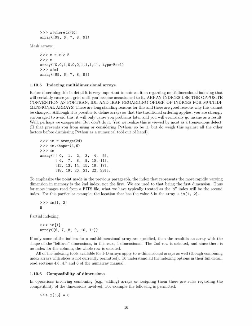
1.10.5 Indexing multidimensional arrays

Before describing this in detail it is very important to note an item regarding multidimensional indexing thatwill certainly cause you grief until you become accustomed to it. ARRAY INDICES USE THE OPPOSITECONVENTION AS FORTRAN, IDL AND IRAF REGARDING ORDER OF INDICES FOR MULTIDI-MENSIONAL ARRAYS! There are long standing reasons for this and there are good reasons why this cannotbe changed. Although it is possible to define arrays so that the traditional ordering applies, you are stronglyencouraged to avoid this; it will only cause you problems later and you will eventually go insane as a result.Well, perhaps we exaggerate. But don’t do it. Yes, we realize this is viewed by most as a tremendous defect.(If that prevents you from using or considering Python, so be it, but do weigh this against all the otherfactors before dismissing Python as a numerical tool out of hand).

> > > im = arange(24)> > > im.shape=(4,6)> > > imarray([[ 0, 1, 2, 3, 4, 5],

[ 6, 7, 8, 9, 10, 11],[12, 13, 14, 15, 16, 17],[18, 19, 20, 21, 22, 23]])

To emphasize the point made in the previous paragraph, the index that represents the most rapidly varyingdimension in memory is the 2nd index, not the first. We are used to that being the first dimension. Thusfor most images read from a FITS file, what we have typically treated as the “x” index will be the secondindex. For this particular example, the location that has the value 8 in the array is im[1, 2].

> > > im[1, 2]8

Partial indexing:

> > > im[1]array([6, 7, 8, 9, 10, 11])

If only some of the indices for a multidimensional array are specified, then the result is an array with theshape of the “leftover” dimensions, in this case, 1-dimensional. The 2nd row is selected, and since there isno index for the column, the whole row is selected.

All of the indexing tools available for 1-D arrays apply to n-dimensional arrays as well (though combiningindex arrays with slices is not currently permitted). To understand all the indexing options in their full detail,read sections 4.6, 4.7 and 6 of the numarray manual.

1.10.6 Compatibility of dimensions

In operations involving combining (e.g., adding) arrays or assigning them there are rules regarding thecompatibility of the dimensions involved. For example the following is permitted:

> > > x[:5] = 0

16

since a single value is considered “broadcastable” over a 5 element array. But this is not permitted:

> > > x[:5] = array([0,1,2,3])

since a 4 element array does not match a 5 element array.The following explanation can probably be skipped by most on the first reading; it is only important to

know that rules for combining arrays of different shapes are quite general. It is hard to precisely specify therules without getting a bit confusing, but it doesn’t take long to get a good intuitive feeling for what is andisn’t permitted. Here’s an attempt anyway: The shapes of the two involved arrays when aligned on theirtrailing part must be equal in value or one must have the value one for that dimension. The following pairsof shapes are compatible:

(5,4):(4,) -> (5,4)(5,1):(4,) -> (5,4)(15,3,5):(15,1,5) -> (15,3,5)(15,3,5):(3,5) -> (15,3,5)(15,1,5):(3,1) -> (15,3,5)

so that one can add arrays of these shapes or assign one to the other (in which case the one being assignedmust be the smaller shape of the two). For the dimensions that have a 1 value that are matched againsta larger number, the values in that dimension are simply repeated. For dimensions that are missing, thesub-array is simply repeated for those. The following shapes are not compatible:

(3,4):(4,3)(1,3):(4,)

Examples:

> > > x = zeros((5,4))> > > x[:,:] = [2,3,2,3]> > > xarray([[2, 3, 2, 3],

[2, 3, 2, 3],[2, 3, 2, 3],[2, 3, 2, 3],[2, 3, 2, 3]])

> > > a = arange(3)> > > b = a[:] # different array, same data (huh?)> > > b.shape = (3,1)> > > barray([[0],

[1],[2]])

> > > a*b # outer productarray([[0, 0, 0],

[0, 1, 2],[0, 2, 4]])

1.10.7 ufuncs

A ufunc (short for Universal Function) applies the same operation or function to all the elements of an arrayindependently. When two arrays are added together, the add ufunc is used to perform the array addition.There are ufuncs for all the common operations and mathematical functions. More specialized ufuncs canbe obtained from add-on libraries. All the operators have corresponding ufuncs that can be used by name(e.g., add for +). These are all listed in table below. Ufuncs also have a few very handy methods for binaryoperators and functions whose use are demonstrated here.

17

> > > x = arange(9)> > > x.shape = (3,3)> > > xarray([0, 1, 2],

[3, 4, 5],[6, 7, 8]])

> > > add.reduce(x) # sums along the first indexarray([9, 12, 15])> > > add.reduce(x, axis=1) # sums along the 2nd indexarray([3, 12, 21])> > > add.accumulate(x) # cumulative sum along the first indexarray([[0, 1, 2],

[3, 5, 7],[9, 12, 15]])

> > > multiply.outer(arange(3),arange(3))array([[0, 0, 0],

[0, 1, 2],[0, 2, 4]])

Standard Ufuncs (with corresponding symbolic operators, when they exist, shown in parentheses)add (+) log greater (>)subtract (-) log10 greater_equal (>=)multiply (*) cos less (<)divide (/) arcos less_equal (<=)remainder (%) sin logical_andabsolute, abs arcsin logical_orfloor tan logical_xorceil arctan bitwise_and (&)fmod cosh bitwise_or (|)conjugate sinh bitwise_xor (^)minimum tanh bitwise_not (~)maximum sqrt rshift (>>)power (**) equal (==) lshift (<<)exp not_equal (!=)

Note that there are no corresponding Python operators for logical_and and logical_or. The Pythonand and or operators are NOT equivalent to these respective ufuncs!

1.10.8 Array functions

There are many array utility functions. The following lists the more useful ones with a one line description.See the numarray manual for details on how they are used. Arguments shown with argument=value indicatewhat the default value is if called without a value for that argument.

all(a): are all elements of array nonzero

allclose(a1, a2, rtol=1.e-5, atol=1.e-8 ): true if all elements within specified amount (between two arrays)

alltrue(a, axis=0 ): are all elements nonzero along specified axis true.

any(a): are any elements of an array nonzero

argmax(a, axis=-1 ), argmin(a,axis=-1 ): return array with min/max locations for selected axis

argsort(a, axis=-1 ): returns indices of results of sort on an array

18

choose(selector, population, clipmode=CLIP): fills specified array by selecting corresponding values from aset of arrays using integer selection array (population is a tuple of arrays; see tutorial 2)

clip(a, amin, amax ): clip values of array a at values amin, amax

dot(a1, a2 ): dot product of arrays a1 & a2

compress(condition, a ,axis=0 ): selects elements from array a based on Boolean array condition

concatenate(arrays, axis=0 ): concatenate arrays contained in sequence of arrays arrays

cumproduct(a, axis=0 ): net cumulative product along specified axis

cumsum(a, axis=0 ): accumulate array along specified axis

diagonal(a, offset=0, axis1=0, axis2=1 ): returns diagonal of 2-d matrix with optional offsets.

fromfile(file, type, shape=None): Use binary data in file to form new array of specified type.

fromstring(datastring, type, shape=None): Use binary data in datastring to form new array of specifiedshape and type

identity(n, type=None): returns identity matrix of size nxn.

indices(shape, type=None): generate array with values corresponding to position of selected index of thearray

innerproduct(a1, a2 ): guess

matrixmultiply(a1, a2 ): guess

outerproduct(a1, a2 ): guess

product(a, axis=0 ): net product of elements along specified axis

ravel(a): creates a 1-d version of an array

repeat(a, repeats, axis=0 ): generates new array with repeated copies of input array a

resize(a, shape): replicate or truncate array to new shape

searchsorted(bin, a): return indices of mapping values of an array a into a monotonic array bin

sometrue(a, axis=0 ): are any elements along specified axis true

sort(a, axis=-1 ): sort array elements along selected axis

sum(a, axis=0 ): sum array along specified axis

swapaxes(a, axis1, axis2 ): switch indices for axis of array (doesn’t actually move data, just maps indicesdifferently)

trace(a, offset=0, axis1=0, axis2=1 ): compute trace of matrix a with optional offset.

transpose(a, axes=None): transpose indices of array (doesn’t actually move data, just maps indices differ-ently)

where(a): find “true” locations in array a

19

1.10.9 Array methods

Arrays have several methods. They are used as methods are with any object. For example (using thearray from the previous example):

> > > # sum all array elements> > > x.sum() # the L indicates a Python Long integer36L

The following lists all the array methods that exist for an array object a (a number are equivalent to arrayfunctions; these have no summary description shown):

a .argmax(axis=-1 )

a .argmin(axis=-1 )

a .argsort(axis=-1 )

a .astype(type): copy array to specified numeric type

a .byteswap(): perform byteswap on data in place

a .byteswapped(): return byteswapped copy of array

a .conjugate(): complex conjugate

a .copy(): produce copied version of array (instead of view)

a .diagonal()

a .info(): print info about array

a .isaligned(): are data elements guaranteed aligned with memory?

a .isbyteswapped(): are data elements in native processor order?

a .iscontiguous(): are data elements contiguous in memory?

a .is_c_array(): are data elements aligned, not byteswapped, and contiguous?

a .is_fortran_contiguous(): are indices defined to follow Fortran conventions?

a .is_f_array(): are indices defined to follow Fortran conventions and data are aligned and not byteswapped

a .itemsize(): size of data element in bytes

a .max(type=None): maximum value in array

a .min(): minimum value in array

a .nelements(): total number of elements in array

a .new(): returns new array of same type and size (data uninitialized)

a .repeat(a,repeats,axis=0):

a .resize(shape):

a .size(): same as nelements

a .type(): returns type of array

a .typecode(): returns corresponding typecode character used by Numeric

a .tofile(file): write binary data to file

a .tolist(): convert data to Python list format

20

a .tostring(): copy binary data to Python string

a .transpose(axes=-1 ): transpose array

a .stddev(): standard deviation

a .sum(): sum of all elements

a .swapaxes(axis1,axis2 )

a .togglebyteorder(): change byteorder flag without changing actual data byteorder

a .trace()

a .view(): returns new array object using view of same data

1.10.10 Array attributes:

a.shape: returns shape of array

a.flat: returns view of array treating it as 1-dimensional. Doesn’t work if array is not contiguous

a.real: return real component of array (exists for all types)

a.imag, a.imaginary: return imaginary component (exists only for complex types)

1.11 ExampleThe following example shows how to use some of these tools. The idea is to select only data within a givenradius of the center of the galaxy displayed and compute the total flux within that radius using the built-inarray facilities.

First we will create a mask for all the pixels within 50 pixels of the center. We begin by creating x andy arrays that whose respective values indicate the x and y locations of pixels in the arrays:

# first find location of maximum in imagey, x = indices(im.shape, type=Float32) # note order of x, y!# after finding peak at 257,258 using ds9x = x-257 # make peak have 0 valuey = y-258radius = sqrt(x**2+y**2)mask = radius < 50display mask*im(mask*im).sum() # sum total of masked image# orim[where(mask)].sum() # sum those points within the radius# look Ma, no loops!

1.12 ExercisesThe needed data for these exercises can be downloaded from stsdas.stsci.edu/python.

1. Start up Python (Python, PyRAF, or IPython). Type print ’hello world’. Don’t go further untilyou master this completely.

2. Read pix.fits, find the value of the OBJECT keyword, and print all the image values in the 10th columnof the image.

3. Scale all the values in the image by 2.3 and store in a new variable. Determine the mean value of thescaled image

21

4. Save the center 128x128 section of the scaled image to a new FITS file using the same header. Itwon’t be necessary to update the NAXIS keywords of the header; that will be handled automaticallyby PyFITS.

5. Extra credit: Create an image (500x500) where the value of the pixels is a Gaussian-weighted sinusoidexpressed by the following expression:

sin(x/π)e−((x−250)2+(y−250)2)/2500.

where x represents the x pixel location and likewise for y. Display it. Looking at the numarraymanual, find out how to perform a 2-D FFT and display the absolute value of the result.

22

2 Reading and plotting spectral dataIn this tutorial we will cover some simple plotting commands using Matplotlib, a Python plotting packagedeveloped by John Hunter of the University of Chicago. We will also talk about reading FITS tables, delvea little deeper into some of Python’s data structures, and use a few more of Python’s features that makecoding in Python so straightforward.

2.1 Example session to read spectrum and plot itThe sequence of commands below represent reading a spectrum from a FITS table and using matplotlib toplot it. Each step will be explained in more detail in following subsections.

> > > import pyfits> > > from pylab import * # import plotting module> > > pyfits.info(’fuse.fits’)> > > tab = pyfits.getdata(’fuse.fits’) # read table> > > tab.names # names of columns> > > tab.formats # formats of columns> > > flux = tab.field(’flux’) # reference flux column> > > wave = tab.field(’wave’)> > > flux.shape # show shape of flux column array> > > plot(wave, flux) # plot flux vs wavelength

# add xlabel using symbols for lambda/angstrom> > > xlabel(r’$\lambda (\angstrom)$’, size=13)> > > ylabel(’Flux’)# Overplot smoothed spectrum as dashed line> > > from numarray.convolve import boxcar> > > sflux = boxcar(flux.flat, (100,)) # smooth flux array> > > plot(wave, sflux, ’--r’, hold=True) # overplot red dashed line> > > subwave = wave.flat[::100] # sample every 100 wavelengths> > > subflux = flix.flat[::100]> > > plot(subwave,subflat,’og’) # overplot points as green circles> > > errorbar(subwave, subflux, yerr=0.05*subflux, fmt=’.k’)> > > legend((’unsmoothed’, ’smoothed’, ’every 100’))> > > text(1007, 0.5, ’Hi There’)

# save to png and postscript files> > > savefig(’fuse.png’)> > > savefig(’fuse.ps’)

2.2 An aside on how Python finds modulesWhen you import a module, how does Python know where to look for it? When you start up Python, thereis a search path defined that you can access using the path attribute of the sys module. So:

> > > import sys> > > sys.path[”, ’C:\\WINNT\\system32\\python23.zip’,’C:\\Documents and Settings\\rij\\SSB\\demo’,’C:\\Python23\\DLLs’, ’C:\\Python23\\lib’,’C:\\Python23\\lib\\plat-win’,’C:\\Python23\\lib\\lib-tk’,’C:\\Python23’,’C:\\Python23\\lib\\site-packages ’,’C:\\Python23\\lib\\site-packages\\Numeric’,’C:\\Python23\\lib\\site-package s\\gtk-2.0’,

23

’C:\\Python23\\lib\\site-packages\\win32’,’C:\\Python23\\lib\\site -packages\\win32\\lib’,’C:\\Python23\\lib\\site-packages\\Pythonwin’]

This is a list of the directories that Python will search when you import a module. If you want to find outwhere Python actually found your imported module, the __file__ attribute shows the location:

> > > pyfits.__file__’C:\\Python23\\lib\\site-packages\\pyfits.pyc’

Note the double ’\’ characters in the file specifications; Python uses \ as its escape character (which meansthat the following character is interpreted in a special way. For example, \n means “newline”, \t means“tab” and \a means “ring the terminal bell”). So if you really want a backslash, you have to escape it withanother backslash. Also note that the extension of the pyfits module is .pyc instead of .py; the .pyc fileis the bytecode compiled version of the .py file that is automatically generated whenever a new version ofthe module is executed.

2.3 Reading FITS table dataAs well as reading regular FITS images, PyFITS also reads tables as arrays of records (recarrays in numarrayparlance). These record arrays may be indexed just like numeric arrays though numeric operations cannotbe performed on the record arrays themselves. All the columns in a table may be accessed as arrays as well.

> > > import pyfits

Assuming a FITS table of FUSE data in the current directory with the imaginative name of ’fuse.fits’

> > > pyfits.info(’fuse.fits’)Filename: fuse.fitsNo. Name Type Cards Dimensions Format0 PRIMARY PrimaryHDU 365 () Int161 SPECTRUM BinTableHDU 35 1R x 7C [10001E,10001E, 10001E, 10001J, 10001E, 10001E, 10001I]> > > tab = pyfits.getdata(’fuse.fits’) # returns table as record array

PyFITS record arrays have a names attribute that contains the names of the different columns of the array(there is also a format attribute that describes the type and contents of each column).

> > > tab.names[’WAVE’, ’FLUX’, ’ERROR’, ’COUNTS’, ’WEIGHTS’, ’BKGD’, ’QUALITY’]> > > tab.formats[’10001Float32’, ’10001Float32’, ’10001Float32’, ’10001Float32’,’10001Float32’, ’10001Float32’, ’10001Int16’]

The latter indicates that each column element contains a 10001 element array of the types indicated.

> > > tab.shape(1,)

The table only has one row. Each of the columns may be accessed as it own array by using the field method.Note that the shape of these column arrays is the combination of the number of rows and the size of thecolumns. Since in this case the columns contain arrays, the result will be two-dimensional (albeit with oneof the dimensions only having length one).

> > > wave = tab.field(’wave’)> > > flux = tab.field(’flux’)> > > flux.shape(1, 10001)

24

The arrays obtained by the field method are not copies of the table data, but instead are views into therecord array. If one modifies the contents of the array, then the table itself has changed. Likewise, if a record(i.e., row) of the record array is modified, the corresponding column array will change. This is best shownwith a different table:

> > > tab2 = getdata(’table2.fits’)> > > tab2.shape # how many rows?(3,)> > > tab2array([(’M51’, 13.5, 2),(’NGC4151’, 5.7999999999999998, 5),(’Crab Nebula’, 11.119999999999999, 3)],formats=[’1a13’, ’1Float64’, ’1Int16’],shape=3,names=[’targname’, ’flux’, ’nobs’])> > > col3 = tab2.field(’nobs’)> > > col3array([2, 5, 3], type=Int16)> > > col1[2] = 99> > > tab2array([(’M51’, 13.5, 2),(’NGC4151’, 5.7999999999999998, 5),(’Crab Nebula’, 11.119999999999999, 99)],formats=[’1a13’, ’1Float64’, ’1Int16’],shape=3,names=[’targname’, ’flux’, ’nobs’])

Numeric column arrays may be treated just like any other numarray array. Columns that contain characterfields are returned as character arrays (with their own methods, described in the PyFITS User Manual)

Updated or modified tables can be written to FITS files using the same functions as for image or arraydata.

2.4 Quick introduction to plottingThe package matplotlib is used to plot arrays and display image data. This section gives a few examplesof how to make quick plots. More examples will appear later in the tutorial (these plots assume that the.matplotlibrc file has been properly configured; the default version at STScI has been set up that way.There will be more information about the .matplotlibrc file later in the tutorial).

First, we must import the functional interface to matplotlib

> > > from pylab import *

2.4.1 Simple x-y plots

To plot flux vs wavelength:

> > > plot(wave, flux)[<matplotlib.lines.Line2D instance at 0x02A07440>]

25

Note that the resulting plot is interactive. The toolbar at the bottom is used for a number of actions.The button with arrows arranged in a cross pattern is used for panning or zooming the plot. In this modethe zooming is accomplished by using the middle mouse button; dragging it in the x direction affects thezoom in that direction and likewise for the y direction. The button with a magnifying glass and rectangleis used for the familiar zoom to rectangle (use the left mouse button to drag define a rectangle that will bethe new view region for the plot. The left and right arrow buttons can be used to restore different views ofthe plot (a history is kept of every zoom and pan). The button with a house will return it the the originalview. The button with a diskette allows one to save the plot to a .png or postscript file. You can resize thewindow and the plot will re-adjust to the new window size.

Also note that this and many of the other pylab commands result in a cryptic printout. That’s becausethese function calls return a value. In Python when you are in an interactive mode, the act of entering avalue at the command line, whether it is a literal value, evaluated expression, or return value of a function,Python attempts to print out some information on it. Sometimes that shows you the value of the object(if it is simple enough) like for numeric values or strings, or sometimes it just shows the type of the object,which is what is being shown here. The functions return a value so that you can assign it to a variable tomanipulate the plot later (it’s not necessary to do that though, though for now it does help keep the screenuncluttered). We are likely to change the behavior of the object so that nothing is printed (even though itis still returned) so your session screen will not be cluttered with these messages.

2.4.2 Labeling plot axes

It is possible to customize plots in many ways. This section will just illustrate a few possibilities

> > > xlabel(r’$\lambda (\angstrom)$’, size=13)<matplotlib.text.Text instance at 0x029A9F30>

26

> > > ylabel(’Flux’)<matplotlib.text.Text instance at 0x02A07BC0>

9 8 0 1 0 0 0 1 0 2 0 1 0 4 0 1 0 6 0 1 0 8 0 1 1 0 0)

◦A(λ

01 e 1 22 e 1 23 e 1 24 e 1 25 e 1 26 e 1 2Fl ux

One can add standard axis labels. This example shows that it is possible to use special symbols usingTEX notation.

2.4.3 Overplotting

Overplots are possible. First we make a smoothed spectrum to overplot.

> > > from numarray.convolve import boxcar # yet another way to import functions> > > sflux = boxcar(flux.flat, (100,)) # smooth flux array using size 100 box> > > plot(wave, sflux, ’--r’, hold=True) # overplot red dashed line[<matplotlib.lines.Line2D instance at 0x0461FC60>]

This example shows that one can use the hold keyword to overplot, and how to use different colors andlinestyles. This case uses a terse representation (-- for dashed and r for red) to set the values, but thereare more verbose ways to set these attributes. As an aside, the function that matplotlib uses are closelypatterned after Matlab. Next we subsample the array to overplot circles and error bars for just those points.

> > > subwave = wave.flat[::100] # sample every 100 wavelengths> > > subflux = flux.flat[::100]> > > plot(subwave,subflat,’og’, hold=True) # overplot points as green circles[<matplotlib.lines.Line2D instance at 0x046EBE40>]> > > error = tab.field(’error’)> > > suberror = error.flat[::100]

27

> > > errorbar(subwave, subflux, suberror, fmt=’.k’, hold=True)(<matplotlib.lines.Line2D instance at 0x046EBEE0>, <a list of 204 Line2D errorbar objects>)

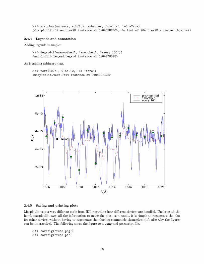
2.4.4 Legends and annotation

Adding legends is simple:

> > > legend((’unsmoothed’, ’smoothed’, ’every 100’))<matplotlib.legend.Legend instance at 0x04978D28>

As is adding arbitrary text.

> > > text(1007., 0.5e-12, ’Hi There’)<matplotlib.text.Text instance at 0x04B27328>

1 0 0 6 1 0 0 8 1 0 1 0 1 0 1 2 1 0 1 4 1 0 1 6 1 0 1 8 1 0 2 0)

◦A(λ

2 e � 1 34 e � 1 36 e � 1 38 e � 1 31 e � 1 2Fl ux H i T h e r e

u n s m o o t h e ds m o o t h e de v e r y 1 0 0

2.4.5 Saving and printing plots

Matplotlib uses a very different style from IDL regarding how different devices are handled. Underneath thehood, matplotlib saves all the information to make the plot; as a result, it is simple to regenerate the plotfor other devices without having to regenerate the plotting commands themselves (it’s also why the figurescan be interactive). The following saves the figure to a .png and postscript file.

> > > savefig(’fuse.png’)> > > savefig(’fuse.ps’)

28

2.5 A little background on Python sequencesPython has a few, powerful built-in “sequence” data types that are widely used. You have already encountered3 of them: strings, lists and tuples.

2.5.1 Strings

Strings are so ubiquitous, that it may seem strange treating them as a special data structure. That theyshare much with the other two (and arrays) will be come clearer soon. First we’ll note here that there areseveral ways to define literal strings. One can define them in the ordinary sense using either single quotes(’) or double quotes ("). Furthermore, one can define multi-line strings using triple single or double quotesto start and end the string. For example:

> > > s = ”’This is an exampleof a multi-line string thatgoes on and on and on.”’> > > s’This is an example\nof a string that\ngoes on and on\nand on’> > > print sThis is an exampleof a string thatgoes on and onand on

As with C, one uses the backslash character in combination with others to denote special characters. Themost common is \n for new line (which means one uses \\ to indicate a single \ is desired). See the Pythondocumentation for the full set. For certain cases (like regular expressions or MS Windows path names), itis more desirable to avoid special interpretation of backslashes. This is accomplished by prefacing the stringwith an r (for ’raw’ mode):

> > > print ’two lines \n in this example’two linesin this example> > > print r’but not \n this one’but not \n this one

Strings are full fledged Python objects with many useful methods for manipulating them. The following isa brief list of all those available with a few examples illustrating their use. Details on their use can be foundin the Python library documentation, the references in Appendix A or any introductory Python book. Notethat optional arguments are enclosed in square brackets. For a given string s :

s .capitalize(): capitalize first character

s .center(width [,fillchar]): return string centered in string of width specified with optional fill char

s .count(sub [,start[,end]]): return number of occurrences of substring

s .decode([encoding [,errors]]): see documentation

s .encode([encoding [,errors]]): see documentation

s .endswith(suffix [,start [,end]]): True if string ends with suffix

s .expandtabs([tabsize]): defaults to 8 spaces

s .find(substring[,start [,end]]): returns position of substring found

s .index(substring[,start [,end]]): like find but raises exception on failure

29

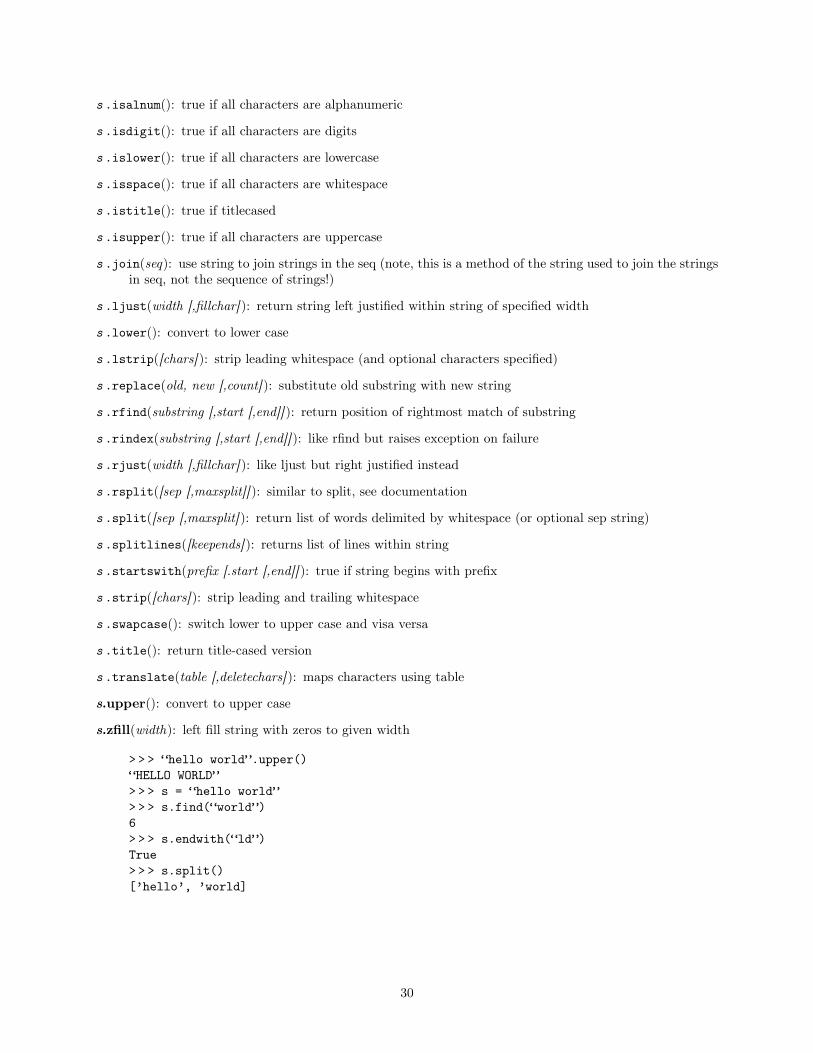
s .isalnum(): true if all characters are alphanumeric

s .isdigit(): true if all characters are digits

s .islower(): true if all characters are lowercase

s .isspace(): true if all characters are whitespace

s .istitle(): true if titlecased

s .isupper(): true if all characters are uppercase

s .join(seq): use string to join strings in the seq (note, this is a method of the string used to join the stringsin seq, not the sequence of strings!)

s .ljust(width [,fillchar]): return string left justified within string of specified width

s .lower(): convert to lower case

s .lstrip([chars]): strip leading whitespace (and optional characters specified)

s .replace(old, new [,count]): substitute old substring with new string

s .rfind(substring [,start [,end]]): return position of rightmost match of substring

s .rindex(substring [,start [,end]]): like rfind but raises exception on failure

s .rjust(width [,fillchar]): like ljust but right justified instead

s .rsplit([sep [,maxsplit]]): similar to split, see documentation

s .split([sep [,maxsplit]): return list of words delimited by whitespace (or optional sep string)

s .splitlines([keepends]): returns list of lines within string

s .startswith(prefix [.start [,end]]): true if string begins with prefix

s .strip([chars]): strip leading and trailing whitespace

s .swapcase(): switch lower to upper case and visa versa

s .title(): return title-cased version

s .translate(table [,deletechars]): maps characters using table

s.upper(): convert to upper case

s.zfill(width): left fill string with zeros to given width

> > > “hello world”.upper()“HELLO WORLD”> > > s = “hello world”> > > s.find(“world”)6> > > s.endwith(“ld”)True> > > s.split()[’hello’, ’world]

30

2.5.2 Lists

Think of lists as one-dimensional arrays that can contain anything for its elements. Unlike arrays, theelements of a list can be different kinds of objects (including other lists) and the list can change in size. Listsare created using simple brackets, e.g.:

> > > mylist = [1, ’hello’, [2,3]]

This particular list contains 3 objects, the integer value 1, the string ’hello’ and the list [2, 3].Empty lists are permitted:

> > > mylist = []

Lists also have several methods:

l .append(x ): adds x to the end of the list

l .extend(x ): concatenate the list x to the list

l .count(x ): return number of elements equal to x

l .index(x [,i [,j]]): return location of first item equal to x

l .insert(i, x ): insert x at ith position

l .pop([i]): return last item [or ith item] and remove it from the list

l .remove(x ): remove first occurrence of x from list

l .reverse(): reverse elements in place

l .sort([cmp [,key [,reverse]]]): sort the list in place (how sorts on disparate types are handled are describedin the documentation)

2.5.3 Tuples

One can view tuples as just like lists in some respects. They are created from lists of items within a pair ofparentheses. For example:

> > > mytuple = (1, “hello”, [2,3])

Because parentheses are also used in expressions, there is the odd case of creating a tuple with only oneelement:

> > > mytuple = (2) # not a tuple!

doesn’t work since (2) is evaluated as the integer 2 instead of a tuple. For single element tuples it is necessaryto follow the element with a comma:

> > > mytuple = (2,) # this is a tuple

Likewise, empty tuples are permitted:

> > > mytuple = ()

If tuples are a lot like lists why are they needed? They differ in one important characteristic (why this isneeded won’t be explained here, just take our word for it). They cannot be changed once created; they arecalled immutable. Once that “list” of items is identified, that list remains unchanged (if the list containsmutable things like lists, it is possible to change the contents of mutable things within a tuple, but you can’tremove that mutable item from the tuple). Tuples have no standard methods.

31

2.5.4 Standard operations on sequences

Sequences may be indexed and sliced just like arrays:

> > > s[0]’h’> > > mylist2 = mylist[1:]> > > mylist2[“hello”, [2, 3]]

Note that unlike arrays, slices produce a new copy.Likewise, index and slice assignment are permitted for lists (but not for tuples or strings, which are also

immutable)

> > > mylist[0] = 99> > > mylist[99, “hello”, [2, 3]]> > > mylist2[1, “hello”, [2,3]] # note change doesn’t appear on copy> > > mylist[1:2] = [2,3,4]> > > mylist[1, 2, 3, 4, [2, 3]]

Note that unlike arrays, slices may be assigned a different sized element. The list is suitably resized.There are many built-in functions that work with sequences. An important one is len() which returns

the length of the sequence. E.g,

> > > len(s)11

This function works on arrays as well (arrays are also sequences), but it will only return the length of thenext dimension, not the total size:

> > > x = array([[1,2],[3,4]])> > > print x[[1 2][3 4]]> > > len(x)2

For strings, lists and tuples, adding them concatenates them, multiplying them by an integer is equivalentto adding them that many times. All these operations result in new strings, lists, and tuples.

> > > ’hello ’+’world’’hello world’> > > [1,2,3]+[4,5][1,2,3,4,5]> > > 5*’hello ’’hello hello hello hello hello ’

2.5.5 Dictionaries

Lists, strings and tuples are probably somewhat familiar to most of you. They look a bit like arrays, in thatthey have a certain number of elements in a sequence, and you can refer to each element of the sequence byusing its index. Lists and tuples behave very much like arrays of pointers, where the pointers can point tointegers, floating point values, strings, lists, etc. The methods allow one to do the kinds of things you need

32

to do to arrays; insert/delete elements, replace elements of one type with another, count them, iterate overthem, access them sequentially or directly, etc.

Dictionaries are different. Dictionaries define a mapping between a key and a value. The key can be eithera string, an integer, a floating point number or a tuple (technically, it must be immutable, or unchangeable),but not a list, dictionary, array or other mutable objects, while the value has no limitations. So, here’s adictionary:

> > > thisdict = {’a’:26.7, 1:[’random string’, 66.4], -6.3:”}

As dictionaries go, this one is pretty useless. There’s a key whose name is the string ’a’, with the floatingpoint value of 26.7. The second key is the integer 1, and its value is the list containing a string and afloating point value. The third key is the floating point number -6.3, with the empty string as its value.Dictionaries are examples of a mapping data type, or associative array. The order of the key/value pairs inthe dictionary is not related to the order in which the entries were accumulated; the only thing that mattersis the association between the key and the value. So dictionaries are great for, for example, holding IRAFparameter/value sets, associating numbers with filter names, and passing keyword/value pairs to functions.Like lists, they have a number of built-in methods:

d .copy(): Returns a shallow copy of the dictionary (subtleties of copies will be addressed in tutorial 4)

d .has_key(k): Returns True if key k is in d, otherwise False

d .items(): Returns a list of all the key/value pairs

d .keys(): Returns a list of all the keys

d .values(): Returns a list of all the values

d .iteritems(): Returns an iterator on all items

d .iterkeys(): Returns an iterator an all keys

d .itervalues(): Returns an iterator on all keys

d .get(k [,x]): Returns d[k] if k is in d, otherwise x

d .clear(): Removes all items

d .update(D): For each k in dictionary D, sets (or adds) k of dictionary = D[k]

d .setdefault(k [,x]): Returns value of k if k is in dictionary, otherwise creates key k, sets value to x, andreturns x

d .popitem(): Removes and returns an arbitrary item

So, for example, we could store the ACS photometric zeropoints in a dictionary where the key is the nameof the filter:

> > > zeropoints = {’F435W’:25.779, ’F475W’:26.168, ’F502N’:22.352, ’F550M’:24.867,’F555W’:25.724, ’F606W’:26.398, ’F625W’:25.731, ’F658N’:22.365, ’F660N’:21.389,’F775W’:25.256, ’F814W’:25.501, ’F850LP’:24.326, ’F892N’:21.865}> > > filter = hdr[’filter1’]> > > if filter.find(’CLEAR’) != -1: filter = hdr[’filter2’]> > > zp = zeropoints[filter]

Dictionaries are very powerful; if your programs do not use them regularly, you are likely doing somethingvery wrong.

The power afforded by dictionaries, lists, tuples and strings and their built-in methods is one of the greatstrengths of Python.

33

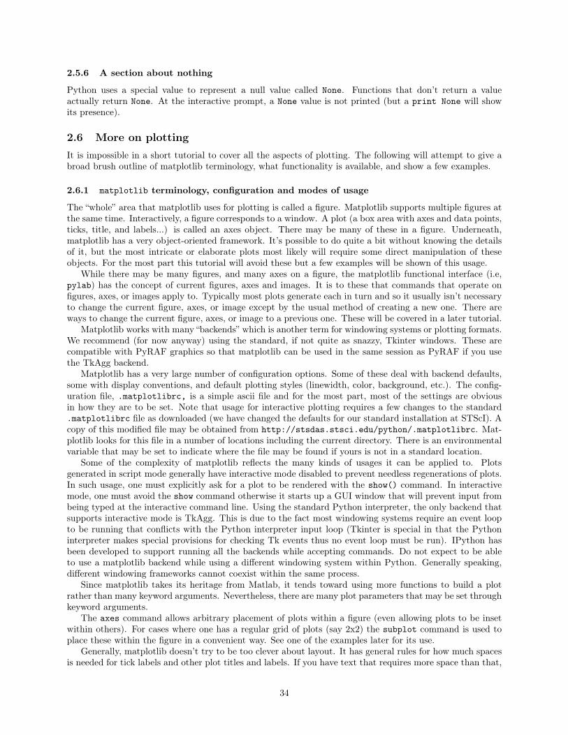
2.5.6 A section about nothing

Python uses a special value to represent a null value called None. Functions that don’t return a valueactually return None. At the interactive prompt, a None value is not printed (but a print None will showits presence).

2.6 More on plottingIt is impossible in a short tutorial to cover all the aspects of plotting. The following will attempt to give abroad brush outline of matplotlib terminology, what functionality is available, and show a few examples.

2.6.1 matplotlib terminology, configuration and modes of usage

The “whole” area that matplotlib uses for plotting is called a figure. Matplotlib supports multiple figures atthe same time. Interactively, a figure corresponds to a window. A plot (a box area with axes and data points,ticks, title, and labels...) is called an axes object. There may be many of these in a figure. Underneath,matplotlib has a very object-oriented framework. It’s possible to do quite a bit without knowing the detailsof it, but the most intricate or elaborate plots most likely will require some direct manipulation of theseobjects. For the most part this tutorial will avoid these but a few examples will be shown of this usage.

While there may be many figures, and many axes on a figure, the matplotlib functional interface (i.e,pylab) has the concept of current figures, axes and images. It is to these that commands that operate onfigures, axes, or images apply to. Typically most plots generate each in turn and so it usually isn’t necessaryto change the current figure, axes, or image except by the usual method of creating a new one. There areways to change the current figure, axes, or image to a previous one. These will be covered in a later tutorial.

Matplotlib works with many “backends” which is another term for windowing systems or plotting formats.We recommend (for now anyway) using the standard, if not quite as snazzy, Tkinter windows. These arecompatible with PyRAF graphics so that matplotlib can be used in the same session as PyRAF if you usethe TkAgg backend.

Matplotlib has a very large number of configuration options. Some of these deal with backend defaults,some with display conventions, and default plotting styles (linewidth, color, background, etc.). The config-uration file, .matplotlibrc, is a simple ascii file and for the most part, most of the settings are obviousin how they are to be set. Note that usage for interactive plotting requires a few changes to the standard.matplotlibrc file as downloaded (we have changed the defaults for our standard installation at STScI). Acopy of this modified file may be obtained from http://stsdas.stsci.edu/python/.matplotlibrc. Mat-plotlib looks for this file in a number of locations including the current directory. There is an environmentalvariable that may be set to indicate where the file may be found if yours is not in a standard location.

Some of the complexity of matplotlib reflects the many kinds of usages it can be applied to. Plotsgenerated in script mode generally have interactive mode disabled to prevent needless regenerations of plots.In such usage, one must explicitly ask for a plot to be rendered with the show() command. In interactivemode, one must avoid the show command otherwise it starts up a GUI window that will prevent input frombeing typed at the interactive command line. Using the standard Python interpreter, the only backend thatsupports interactive mode is TkAgg. This is due to the fact most windowing systems require an event loopto be running that conflicts with the Python interpreter input loop (Tkinter is special in that the Pythoninterpreter makes special provisions for checking Tk events thus no event loop must be run). IPython hasbeen developed to support running all the backends while accepting commands. Do not expect to be ableto use a matplotlib backend while using a different windowing system within Python. Generally speaking,different windowing frameworks cannot coexist within the same process.

Since matplotlib takes its heritage from Matlab, it tends toward using more functions to build a plotrather than many keyword arguments. Nevertheless, there are many plot parameters that may be set throughkeyword arguments.

The axes command allows arbitrary placement of plots within a figure (even allowing plots to be insetwithin others). For cases where one has a regular grid of plots (say 2x2) the subplot command is used toplace these within the figure in a convenient way. See one of the examples later for its use.

Generally, matplotlib doesn’t try to be too clever about layout. It has general rules for how much spacesis needed for tick labels and other plot titles and labels. If you have text that requires more space than that,

34

It’s up to you to replot with suitable adjustments to the parameters.Because of the way that matplotlib renders interactive graphics (by drawing to internal memory and

then moving to a display window), it is slow to display over networks (impossible over dial-ups, slow overbroadband; gigabit networks are quite usable however)

2.6.2 matplot functions

The following lists most of the functions available within pylab for quick perusal followed by several examples.

basic plot types (with associated modifying functions)

bar: bar charts

barh: horizontal bar charts

boxplot: box and whisker plots

contour:

contourf: filled contours

errorbar: errorbar plot

hist: histogram plot

implot: display image within axes boundaries (resamples image)

loglog: log log plot

plot: x, y plots

pie

polar

quiver: vector field plot

scatter

semilogx: log x, linear y, x y plot

semilogy: linear x, log y, x y plot

stem

spy: plot sparsity pattern using markers

spy2: plot sparsity pattern using image

plot decorators and modifiers

axhline: plot horizontal line across axes

axvline: plot vertical line across axes

axhspan: plot horizontal bar across axes

axvspan: plot vertical bar across axes

clabel: label contour lines

clim: adjust color limits of current image

grid: set whether grids are visible

legend: add legend to current axes

rgrids: customize the radial grids and labels for polar plots

table: add table to axes

text: add text to axes

thetagrids: for polar plots

title: add title to axes

35

xlabel: add x axes label

ylabel: add y axes label

xlim: set/get x axes limits

ylim: set/get y axes limits

xticks: set/get x ticks

yticks: set/get y ticks

figure functions

colorbar: add colorbar to current figure

figimage: display unresampled image in figure

figlegend: display legend for figure

figtext: add text to figure

object creation/modification/mode/info functions

axes: create axes object on current figure

cla: clear current axes

clf: clear current figure

close: close a figure window

delaxes: delete axes object from the current figure

draw: force a redraw of the current figure

gca: get the current axes object

gcf: get the current figure

gci: get the current image

hold: set the hold state (overdraw or clear?)

ioff: set interactive mode off

ion: set interactive mode on

isinteractive: test for interactive mode

ishold: test for hold mode

rc: control the default parameters

subplot: create an axes within a grid of axes

color table functions

autumn, bone, cool, copper, flag, gray, hot, hsv, pink, prism, spring, summer, winter

2.7 Plotting mini-Cookbook2.7.1 customizing standard plots

The two tables below list the properties of data and text properties and information about what values theycan take. The variants shown in parentheses indicate acceptable abbreviations when used as keywords.

36

Data propertiesProperty Valuealpha Alpha transparency (between 0. and 1., inclusive)antialiased (aa) Use antialiased rendering (True or False)color (c) Style 1:

’b’ -> blue’g’ -> green’r’ -> red’c’ -> cyan’m’ -> magenta’y’ -> yellow’k’ -> black’w’ -> whiteStyle 2: standard color string, eg. ’yellow’, ’wheat’Style 3: grayscale intensity (between 0. and 1., inclusive)Style 4: RGB hex color triple, eg. #2F4F4FStyle 5: RGB tuple, e.g., (0.18, 0.31, 0.31), all values be-tween 0. and 1.)

data_clipping Clip data before plotting (if the great majority of pointswill fall outside the plot window this may be much faster);True or False

label A string optionally used for legendlinestyle (ls) One of ’–’ (dashed), ’:’ (dotted), ’-.’ (dashed dot), ’-’ solidlinewidth (lw) width of line in points (nonzero float value)marker symbol:

’o’ -> circle’^’,’v’,’<’,’>’ triangles: up, down, left, right respectively’s’ -> square’+’ -> plus’x’ -> cross’D’ -> diamond’d’ -> thin diamond’1’,’2’,’3’,’4’ tripods: down, up, left, right’h’ -> hexagon’p’ -> pentagon’|’ -> vertical line’_’ -> horizontal line’steps’ (keyword arg only)

markeredgewidth (mew) width in points (nonzero float value)markeredgecolor (mec) color valuemarkerfacecolor (mef) color valuemarkersize (ms) size in points (nonzero float value)

37

The following describes text attributes (those shared with lines are not detailed)

Property Valuealpha, color As with Linesfamily font family, eg ’sans-serif’,’cursive’,’fantasy’fontangle the font slant, ’normal’, ’italic’, ’oblique’horizontalalignment ’left’, ’right’, ’center’verticalalignment ’top’, ’bottom’, ’center’multialignment ’left’, ’right’, ’center’ (only for multiline strings)name font name, eg. ’Sans’, ’Courier’, ’Helvetica’position x, y positionvariant font variant, eg. ’normal’, ’small-caps’rotation angle in degrees for text orientationsize size in pointsstyle ’normal’, ’italic’, or ’oblique’text the text string itselfweight e.g ’normal’, ’bold’, ’heavy’, ’light’

These two sets of properties are the most ubiquitous. Others tend to be specialized to a specific taskor function. The following illustrates with some examples (plots are not shown) starting with the ways ofspecifying red for a plotline

> > > x = arange(100.)> > > y = (x/100.)**2> > > plot(x,y,’r’)> > > plot(x,y, c=’red’)> > > plot(x,y, color=’#ff0000’)> > > lines = plot(x,y) # lines is a list of objects, each has set methods

for each property> > > set(lines, ’color’, (1.,0,0)) # or> > > lines[0].set_color(’red’) ; draw() # object manipulation example> > > plot(y[::10], ’g>:’,markersize=20’) # every 10 points with large green triangles and

dotted line

And more examples specifying text:

> > > textobj = xlabel(’hello’, color=’red’,ha=’right’)> > > set(textobj, ’color’, ’wheat’) # change color> > > set(textobj, ’size’, 5) # change size

2.7.2 implot example

You can duplicate simple use of the IRAF task implot like this:

> > > pixdata = pyfits.getdata(’pix.fits’)> > > plot(pixdata[100], hold=False) # plots row 101> > > plot(pixdata[:,200],hold=True) #overplots col 201

38

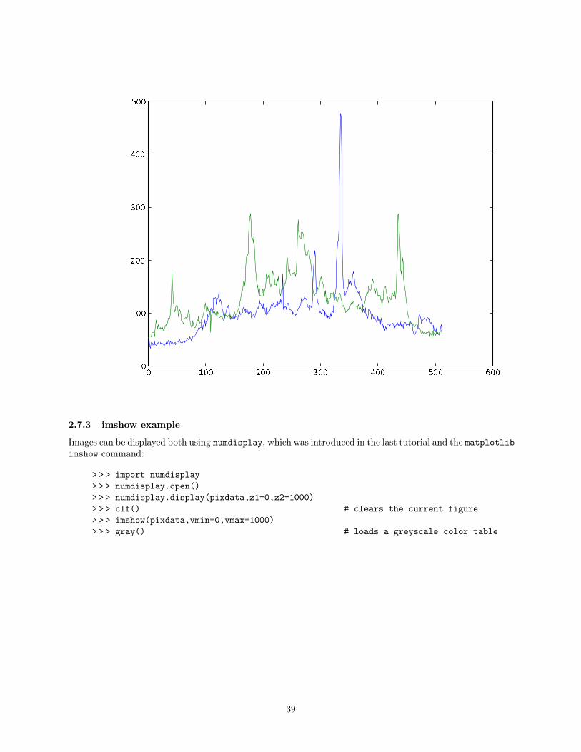
0 1 0 0 2 0 0 3 0 0 4 0 0 5 0 0 6 0 001 0 02 0 03 0 04 0 05 0 0

2.7.3 imshow example

Images can be displayed both using numdisplay, which was introduced in the last tutorial and the matplotlibimshow command:

> > > import numdisplay> > > numdisplay.open()> > > numdisplay.display(pixdata,z1=0,z2=1000)> > > clf() # clears the current figure> > > imshow(pixdata,vmin=0,vmax=1000)> > > gray() # loads a greyscale color table

39

0 1 0 0 2 0 0 3 0 0 4 0 0 5 0 001 0 02 0 03 0 04 0 05 0 0

The default type of display in Matplotlib “out of the box” has the Y coordinate increasing from top tobottom. This behavior can be overridden by changing a line in the .matplotlibrc file:

image.origin : lower

The .matplotlibrc that is the default on STScI unix systems (Solaris, Linux and Mac) has this already setup. If you are using Windows, you will need to get the STScI default .matplotlibrc from one of the Unixsystems, or from the web.

imshow will resample the data to fit into the figure using a defined interpolation scheme. The defaultis set by the image.interpolation parameter in the .matplotlibrc file (bilinear on STScI systems),but this can be set to one of bicubic, bilinear, blackman100, blackman256, blackman64, nearest,sinc144, sinc256, sinc64, spline16 and spline36. Most astronomers are used to blocky pixels thatcome from using the nearest pixel; so we can get this at run-time by doing

> > > imshow(pixdata, vmin=0, vmax=1000, interpolation=’nearest’)

2.7.4 figimage

figimage is like imshow, except no spatial resampling is performed. It also allows displaying RGB or RGB-alpha images. This function behaves more like the IDL TVSCL command. See the manual for more details.

2.7.5 histogram example

Histograms can be plotted using the hist command.

40

> > > pixdata[pixdata>256] = 256> > > hist(pixdata,bins=256)

Duplicating the functionality of, for example, the IRAF imhistogram task will take a bit more work.

� 5 0 0 5 0 1 0 0 1 5 0 2 0 0 2 5 0 3 0 001 0 0 02 0 0 03 0 0 04 0 0 05 0 0 06 0 0 07 0 0 08 0 0 0

2.7.6 contour example

To overplot green contours at levels of 100, 200, 400 and 800, we can do:

> > > levels = [100,200,400,800]> > > imshow(pixdata,vmin=0,vmax=1000,origin=’lower’)> > > contour(pixdata,levels,colors=[1., 1., 1., 0.])

41

0 1 0 0 2 0 0 3 0 0 4 0 0 5 0 001 0 02 0 03 0 04 0 05 0 0

2.7.7 subplot example

You aren’t limited to having one plot per page. The subplot command will divide the page into a user-specified number of plots:

> > > err = err*1.0e12> > > flux = flux*1.0e12

There’s a bug in the axes code of Matplotlib that causes an exception when the upper and lower limits ofthe plot are too close to each other, so we multiply the data by 1.0e12 to guard against this.

> > > subplot(211) # Divide area into 2 vertically, 1horizontally and select the first plot

> > > plot(wavelength,flux)> > > subplot(212) # Select second plot> > > plot(wavelength,error)

42

9 8 0 1 0 0 0 1 0 2 0 1 0 4 0 1 0 6 0 1 0 8 0 1 1 0 0� 10 12 34 56

9 8 0 1 0 0 0 1 0 2 0 1 0 4 0 1 0 6 0 1 0 8 0 1 1 0 000 . 0 50 . 10 . 1 50 . 22.7.8 readcursor example

Finally, it is possible to set up functions to interact with a plot using the event handling capabilities ofMatplotlib. Like many other GUIs, Matplotlib provides an interface to the underlying GUI event handlingmechanism. This is achieved using a callback function that is activated when a certain prescribed action isperformed. The prescribed action could be a mouse button click, key press or mouse movement. You canset up a handler function to handle the event by registering the event you want to detect, and connectingyour callback function with the required event. This is getting a little bit ahead of ourselves here, since weweren’t going to explain functions until the fourth tutorial, but it’s impossible to explain event handlingwithout it....

This is best explained using an example. Say you want to print the X and Y coordinates when you clickthe mouse in an image. Start by displaying the image in an imshow() window:

> > > imshow(pixdata, vmin=0, vmax=200)

Then set up a handler to print out the X and Y coordinates. This will be run every time the mouse buttonis clicked, until the “listener” function is killed.

> > > def clicker(event):... if event.inaxes:... print event.xdata, event.ydata...> > >

43

This is a very simple handler: it just checks whether the cursor is inside the figure (if event.inaxes), andif it it, it prints out the X and Y coordinates in data coordinates (i.e. in the coordinates as specified by theaxes). If the cursor is outside the figure, nothing is done.

Now we set up a “listener” by connecting the event we are looking for (’button_press_event’) with thefunction we will call (clicker).

> > > cid = connect(’button_press_event’, clicker)

The connect function returns a “connect id”, which we will use when we want to kill the listener.Now, when we press the mouse button when we are in the figure, we get the coordinates printed out on

our screen. This works even if we zoom the image, since we have requested the coordinates in data space,so matplotlib takes care of determining the X and Y coordinates correctly for us. When we’re done, we canjust do the following:

> > > disconnect(cid)

and we are no longer listening for button presses.There are more details in the matplotlib manual.

2.8 Exercises1. Using only Python tools, open the FITS file fuse.fits, extract the flux and error columns from

the table, and plot these against each other using plot(). Scale the flux and error by 1.0e12 beforeplotting.

2. Smooth pix.fits with a 31x31 boxcar filter (see first tutorial) and make a contour plot at 90, 70, 50,and 30, and 10% of the peak value of the smoothed image.

3. Repeat 2, except before generating a contour plot display the unsmoothed image underneath.

4. Change the colortable to gray and label your favorite feature with a mathematical expression

5. Save the result as a postscript file and view it in your favorite postscript viewer

6. Extra credit: parroting the readcursor example, write a short callback function to display a cross cutplot of a displayed image on a left mouse button click, and a vertical cut plot on a right button click(overplotting the image). [Hint: this needs use of subplot(111, Frameon=False) to get overplotting onimages to work]

44

3 More advanced topics in PyFITS, numarray and IPython

3.1 IPythonIPython is a souped up interactive environment for Python. It adds many special features to make interactiveanalysis sessions easier and more productive. These features include:

• easy invocation of common shell commands with shell-like syntax (e.g., ls, cd, etc.)

• Alias facility for defining system aliases

• Complete system shell access (through ! and !! prefixes)

• TAB completion

• Easy ways to find out information about modules, functions and objects.

• Numbered input/output prompts with command history

• User-extensible magic commands

• Session logging and restoring (through playback of logged commands)

• Background execution of Python commands in a separate thread

• Automatic indentation

• Macro system

• Auto parenthesis and auto quoting

• Flexible configuration system allowing for multiple configurations

• Easy reimportation (useful for script and module development)

• Easy debugger access

• Syntax highlighting and editor invocation, easier to interpret tracebacks

• Profiler support

This tutorial will only touch a subset of its extensive features (IPython has its own, very complete manual:see Appendix A for instructions on how to obtain it). When started (simply by typing ipython) the mostapparent difference from the standard Python interpreter is the prompt. Each line entered by the user isnumbered. Commands can be recalled through the standard up and down arrow keystrokes (if the readlinelibrary is installed) as well as by number (shown later).

3.1.1 Obtaining information about Python objects and functions

IPython provides a few very handy ways of finding out information about modules, functions, and objects.Some examples:

In [10]: x = [1, 2] # create a short list

Typing ? before or after a name (module, variable, etc.) gives information about that module or objectincluding documentation included in the source code for that module or object (the “docstring”, discussedlater).

45

In [11]: x?Type: listBase Class: <type ’list’>String Form: [1, 2]Namespace?: InteractiveLength: 2Docstring:

list() -> new listlist(sequence) -> new list initialized from sequence’s items

This shows a little info about the object.If one types a TAB character after the object or module name with a period, IPython will list all the

possible contents of that module or object (i.e., its attributes or methods). One can then look at anydocumentation available for these items using the ? feature. E.g.,

In [12]: x.<TAB>x.__add__ x.__iadd__ x.__setattr__x.__class__ x.__imul__ x.__setitem__x.__contains__ x.__init__ x.__setslice__x.__delattr__ x.__iter__ x.__str__x.__delitem__ x.__le__ x.appendx.__delslice__ x.__len__ x.countx.__doc__ x.__lt__ x.extendx.__eq__ x.__mul__ x.indexx.__ge__ x.__ne__ x.insertx.__getattribute__ x.__new__ x.popx.__getitem__ x.__reduce__ x.removex.__getslice__ x.__reduce_ex__ x.reversex.__gt__ x.__repr__ x.sortx.__hash__ x.__rmul__In [13]: x.append?Type: builtin_function_or_methodBase Class: <type ’builtin_function_or_method’>String Form: <built-in method append of list object at 0x15bcff0>Namespace: InteractiveDocstring:

L.append(object) -- append object to end

This lists all the attributes and methods for lists. Generally you should ignore any names that begin withunderscore (the meaning of all these will be explained in the next tutorial). The next inquiry shows thedocstring info for the list append method.

These techniques can be used to inspect what’s available within any Python object or module. Onecaution: objects that use more sophisticated means of handling attributes and methods will generally notshow these by these inspection tools. So just because you don’t see something doesn’t mean it doesn’t exist.A good example is the data attribute for pyfits objects (something that will be covered in this tutorial).There is such an attribute, but it won’t be seen through the TAB completion mechanism here.

3.1.2 Access to the OS shell

Any system shell command may be executed by prepending it with ’ !’ E.g.,

In [14]: !lsnewfile.fits seq.fits pix.fits

46

3.1.3 Magic commands

IPython has what it calls magic commands. These are special commands not normally part of Python. Thefollowing lists the default set. Users may define their own magic commands.

Magic Command ActionExit Exit IPython without confirmationPprint Toggle pretty printing on/offQuit same as Exitalias Define an alias for a system commandautocall Make functions callable without typing parenthesis (de-

fault)autoindent Toggle autoindent on/off (default on)automagic Make magic functions callable without having to type ’%’

(default)bg Run a job in the background, in a separate threadbookmark Manage bookmark system (for directories)cd Change directoriescolor_info Toggle color syntax highlighting (default on)colors switch color schemeconfig Show IPython’s internal configurationdhist Print history of visited directoriesdirs Return current directory stacked Alias to editedit Bring up editor and execute the resulting codeenv List environmental variableshist Print input history, most recent lastlogoff Stop logginglogon Restart logginglogstart Start logginglogstate Print the status of the logging systemlsmagic List currently available magic functionsmacro Define set of input lines as macromagic Print info about magic function systemp Alias for Python print functionpage Pretty print the object and display it through a pagerpdb Control the calling of the pdb interactive debuggerpdef Print the definition header of any callable objectpdoc Print the docstring for an objectpfile Print the file where an object is definedpinfo Provide detailed information about an objectpopd Change to a directory popped off the directory stackprofile Print currently active IPython profileprun Run a statement through the Python code profilerpsource Print source code for objectpushd Push current directory on stack and change directorypwd Return current working directoryr Repeat previous inputrehash Update the alias table with all entries in $PATHrehashx Update the alias table with all executables in $PATHreset Reset the namespace by removing all names defined by

userrun Run the named file inside IPython as a program

47

runlog Run files as logssave Save a set of lines to a given filenamesc Execute a shell command and capture its outputsx Run a shell command and capture its outputsystem_verbose Toggle verbose printing of system commands on and offtime Time execution of a Python statement or expressionunalias Remove aliaswho Print all interactive variables with minimal formattingwho_ls Return sorted list of all interactive variableswhos Like who but with extra info about each variablexmode Switch modes for exception handlers

The use of many of these is fairly obvious; for others consult the IPython documentation on their use.IPython has default aliases for the following system commands: cat, clear, cp, less, mkdir, mv,

rm, rmdir, and many variants on ls (lc, ldir, lf, lk, ll and lx). The magic alias command allowsone to change or add to the list.

IPython saves the history of previous commands from one session to the next (the manual describes howto keep different session histories).

3.1.4 Syntax shortcuts

With autocall mode on, it means that it is not necessary to provide parentheses for functions that aren’tbeing assigned:

In [15]: pyfits.info ’pix.fits’ # instead of pyfits.info(’pix.fits’)------->pyfits.info(’pix.fits’)Filename: pix.fitsNo. Name Type Cards Dimensions Format0 PRIMARY PrimaryHDU 71 (512, 512) Int16

but note that this doesn’t work:

In [16]: im = pyfits.getdata ’pix.fits’__________________________________________________________

File "<console>", line 1im = pyfits.getdata ’pix.data’

SyntaxError: invalid syntax

If one starts a line with a comma, every argument of a function is assumed to be auto quoted. E.g.:

In [17]:,pyfits.info pix.fits------->pyfits.info(’pix.fits’)Filename: pix.fitsNo. Name Type Cards Dimensions Format0 PRIMARY PrimaryHDU 71 (512, 512) Int16In [18]:,print hello-------->print(’hello’)hello

Note also that when IPython does this sort of autotransformation, it prints the command actually executed.What is saved in the log files is the proper Python syntax, not what you typed. For functions that expectstrings only, this allows near shell-like syntax to be used.

48

3.1.5 IPython history features

Typing Control-p (or Control-n) after you typed something at the command line will match the closestprevious (or next) command in the history that matches what you’ve typed.

Previous input commands are available for re-execution (or other manipulation) by accessing specialvariables. The variable In is effectively a list of the previous commands that can be indexed with thenumber that matches the prompt. Slicing works as well. The following example show how to select a set ofprevious lines for re-execution:

In[19]: print 11

In[20]: print 22

In[21]: print 33

In[22]: print 44In [23]: exec In[19:21]+In[22]124

The previous lines are also accessible through variables _i<n> and _ih<n>. E.g.,

In [24]: print _i22print 4

The return value of statements that return a value (and thus often print or display something to the output)are stored in similar variables. The most recent is in a variable _, the next most recent in __, and likewisefor ___. For example:

In[25]: 6+915In[26]: print _15

Since assignments don’t return anything, they are not saved this way. Like input commands, output valuesare saved in Out and can be indexed, or the variables _o<n> or _oh<n>. This feature may use extramemory since it is saving references to things that normally would be deleted so the feature can be turnedoff (see the later discussion on memory usage for a better understanding of what happens).

By defining a .ipythonrc file in each working directory, one can customize what IPython does for asession started in that directory. Additional IPython features will be illustrated throughout the rest of thetutorials.

3.2 Python IntrospectionSnake navel gazing? No, not quite. This term refers to the capabilities that Python provides for findingout information about Python objects from the objects themselves (IPython makes use of these facilities).Python has very extensive tools for doing this. Only a couple of the simplest will be mentioned here.By using the Python dir() function, one can examine the “contents” of various Python entities includingmodules, objects and classes. For example using dir() on a module will list variables, functions, and classesdefined within the module (but not indicate what they are; in the list there is no visual way of distinguishinga function from a variable–except by use of standard naming conventions in some cases). As an example

49

dir(pyfits) lists over a hundred such items. This can be useful if you can’t quite remember the name of amethod or attribute. By itself, don’t expect to understand everything you see (or even most). One can usedir() on these items in turn to find out about them.

The Python function type() can be used on any object to tell you what type it is. From its use you cantell if something is an integer, string, list, function, or specific object.

Every Python module, function, class and method has a provision for a special string that is available forinspection. This string is called the “docstring”. If it exists, it is the __doc__ attribute of the object. Hereare a few examples:

> > > x = [1,2] # a simple python list> > > print x.__doc__list() -> new listlist(sequence) -> new list initialized from sequence’s items

This shows the docstring for the list creator function.

> > > print pyfits.__doc__ # print the pyfits module docstringA module for reading ........> > > print pyfits.getdata.__doc__...

With these few features it is usually possible to find out quite a bit about any object.

3.3 Saving your dataAt the moment, there are no comparable functions to the IDL save and restore commands. There areways of saving and restoring Python objects (which goes by the odd name of pickling) but its use is far frombeing convenient as the IDL save command. We are working on a command to make saving and restoringdata much easier (and similar to how it is done in IDL), but given the richness of the forms that Pythonobjects can be generated, it is not possible to ensure that all objects can be saved. The future commandwill allow saving of all reasonably saveable objects (for example, open files objects cannot be saved).

3.4 Python loops and conditionals3.4.1 The for statement

Like many other languages Python has a for statement. Its use is a little different than most are likely usedto seeing. Here is an example:

> > > pets = [’dog’,’cat’,’gerbil’,’canary’,’goldfish’,’rock’]> > > for pet in pets: print ’I have a pet’, petI have a pet dogI have a pet catI have a pet gerbilI have a pet canaryI have a pet goldfishI have a pet rock

The for pet in pets syntax means that a loop will be performed for each item in the list pets. In order,the item is taken from the list pets, assigned to the variable pet, which can be used within the loop.Anything that is considered a Python sequence can be used after the in. This includes lists, strings, tuples,arrays and anything else (including user-defined objects) that satisfy certain sequence requirements (actually,it’s more general than that, iterator objects, not described here can be use used as well). In fact, the exactsame approach is used for performing “counted” loops:

50

> > > for i in range(3): print i012

The function range(n) effectively generates a list of n integers starting at 0 (it’s the analog of arange(n)).It turns out that it doesn’t actually generate a list that long (so worries about using up lots of memory forperforming a large number of loops are unfounded).

3.4.2 Blocks of code, and indentation

The form of having the code looped over on the same line as the for statement is atypical. Normally thestatements being looped over follow on separate lines. So what is used to delimit these blocks? Begin/endstatements like IDL? Curly braces ({}) like C and Java? No, nothing other than simple indentation. Whencode following a statement that expect a block of code (such as for) is consistently indented more than thestatement starting the block, it is considered to identify the block of code. For example:

> > > for i in range(3):... x = i*i... print x...014

Note that when one is in interactive mode, that using a statement that starts a block causes the interpreterto prompt with ... and typing an empty line terminates the block (that’s not necessary within scriptsor programs, returning to a previous level of indentation or ending the file is sufficient). The amount ofindentation is entirely up to you. It can be 1 space or 40, so long as it is consistent. Tabs may be used, buttheir use is not recommended. If you do use them, use only tabs for indentation. A mixture of tabs andspaces is bound to cause confusion since different tools show tabs with varying amounts of equivalent spaced.Most sensible editors allow tabs to be automatically converted to spaces with the appropriate configuration(the next tutorial will provide information about editors and available features for Python).

This aspect of Python astonishes some, but most that actually try it find it refreshing. The structurethat you see is the real structure of the program. Cutting and pasting such code into different levels ofindentation is not usually a problem if you use an editor that supports changing indentation for multiplelines of code.

3.4.3 Python if statements

Python if statements are simple:

> > > x = 0> > > if x==0:... print “x equals 0”...x equals 0

The if statement allows optional elif (short for “else if”) and else clauses:

> > > if x==1:... print “x equals 1”... elif x==0:... print “x equals 0”... else:... print “x equals something other than 1 or 0”...x equals 0

51

3.4.4 What’s True and what’s False

Python now has explicit True and False values. But it also has standard rules for determining what isconsidered true and false for other data types. Numeric data types are considered false if equal to 0 and truefor all other values. The Python value None is always considered false. Empty sequences and dictionariesare considered false (e.g., the empty string).

> > > if ”: print ’True’ # nothing will be printed...> > > if ’0’: print ’True’...True

As for user-defined objects, Python permits the code to define what is true or not. Or whether a test fortruth is even permitted; numarray arrays may not be used as truth values:

> > > from numarray import *> > > x = arange(9)> > > if x: print ’True’[...]RuntimeError: An array doesn’t make sense as a truth value. Use any(a) or all true(a)

Error!

3.4.5 The in crowd

Another use for the in operator encountered in the for statement is as a test of whether an object is a memberof a sequence. This can considerably simplify logical tests as the following example shows.

> > > if x in [’dog’, ’cat’, ’goldfish’, ’gerbil’, ’canary’]: print x

3.5 Advanced PyFITS TopicsThe PyFITS functions introduced in the first tutorial are sufficient for simple manipulation of FITS files,but if you need to have more control over the handling of the FITS file, you will need to use some of themore advanced features of the module.

3.5.1 Header manipulations

Normally most people will find the means of using and updating headers described in the first tutorialsufficient for most tasks. There are more methods available for header objects that allow adding commentarykeywords (HISTORY, COMMENT, or ’blank’ keywords). The following show their use.

> > > hdr = pyfits.getheader(’pix.fits’)> > > hdr.add_history(’This is a test history card’)> > > hdr.add_comment(’A test comment card’,after=’date’)> > > hdr.add_blank(”,before=’comment’)# To delete a keyword just use the del statement> > > del hdr[’date’]

Note that while headers behave in a number of respects like dictionaries, they aren’t dictionaries and don’tsupport all dictionary methods.

To have complete control over header cards and their placement of header cards it is necessary to accessthe header as a “cardlist” object. With this representation one can use list manipulations to place each cardas desired, and use card methods to control the exact contents of any card. By this interface it is possible

52

to make the card use any string desired, even if it is not legal FITS or one of the standard conventions (towrite such illegal cards into an output file requires specifically instructing the writeto method or functionto force illegal cards into the file; see the following section on noncompliant FITS data).

See the PyFITS documentation for the full set of methods and examples of use.

3.5.2 PyFITS Object Oriented Interface

The object oriented interface permits more flexible handling of FITS files. The object functionality mirrorsthat available from the functions. The chief advantages are:

• Files are not repeatedly opened and closed for each data access (but the objects should be explicitlyclosed now with the close() method).

• Allows creating FITS headers from scratch (i.e., not having to use an existing file’s header).

• There is more flexibility in how data are accessed. One can easily determine how many extensions existand access all the headers directly without making many getheader function calls.

As for the latter, it is possible to read just portions of an image from disk (rather than reading the wholeimage), and it is possible to open files using memory mapping as a data access mode. Consult the PyFITSUser’s Guide for details on how to do both of these.

Simple example:

> > > hdus = pyfits.open(’fuse.fits’) # returns an HDUList object> > > tabhdu = hdus[1] # the table extension> > > hdr = tabhdu.header # getting the header from the HDU> > > tab = tabhdu.data # and the table

The data attribute of the HDU object contains the data regardless of the type of extension (a record arrayfor tables, a simple array for image extensions). The HDUList may be indexed by number or by extensionname (and optionally EXTVER). For example:

> > > hdus = pyfits.open(’acs.fits’)> > > sci = hdus[’sci’,1] # EXTNAME=SCI, EXTVER=1

HDULists can be written to a new file, or updated if the file was opened in update mode.

> > > hdus.writeto(’temp.fits’) # write current form to new file> > > hdus.flush() # update opened file with current form

3.5.3 Controlling memory usage

Offhand, it sounds convenient to read a whole FITS file into memory as an HDUlist in one step, but somemay wonder about the demands this puts on memory. If the file is memory mapped, then that isn’t aproblem. However, if the default mode of using regular I/O to read FITS files is being used it turns outthat only the headers are loaded. Until one actually refers to the data attribute the data are not read intomemory (it’s done with smoke and mirrors). By using this, it is possible to control what is in memory. Thefollowing illustrates how (the next tutorial unveils some of the details of how memory is handled in generalin Python).

> > > ff = pyfits.open(’nicmos.fits’)> > > sum = 0. # plan is to sum all SCI extension images> > > for hdu in ff[1:]: # skip primary... if hdu.header[’extname’].startswith(’SCI’):... sum = sum + hdu.data # now data is read in... hdu.data = None # done with it, delete it from memory> > > ff.close()

53

If the images are too large to comfortably process in memory, the section attribute can be used to readsubsets of the image. An example that sums all the values in sections of an image without loading it all inmemory at once:

> > > ff = pyfits.open(’pix.fits’) # returns an HDUList object> > > hdu = ff[0] # Get first (and only) HDU> > > sum = 0L # for keeping a running sum of all image values> > > # now read data 64 lines at a time (although small, it illustrates the principle)> > > for i in range(8):... subim = hdu.section[i*64:(i+1)*64,:]... sum = sum + subim.sum()...> > > print sum> > > ff.close()

This can be done more elegantly using image iterators described later.HDULists can be created and manipulated entirely in memory without any reference to any input or

output files.PyFITS is also capable of handling variable-length table entries, random groups, and ascii table exten-

sions.

3.5.4 Support for common FITS conventions

PyFITS supports the CONTINUE convention automatically on reading files that use it (this permits theuse of string values longer than permitted in a standard card). To enable its usage in a header just providestring values to keywords that are longer than standard FITS allows. The HIERARCH convention is notyet supported, but will be in the near future. The INHERIT convention is not supported. It is not plannedto be in the base pyfits module but some convenience functions or objects may be provided in the future tosupport it.

3.5.5 Noncompliant FITS data

Normally PyFITS tries to handle FITS files that don’t meet the FITS standard as best it can when readingthem in (and make the most reasonable interpretations possible of any ambiguities). (If users encounterproblems in this regard, particularly with FITS data that is widely used, please let us know so we can adjustPyFITS to handle it). In contrast, PyFITS normally takes a very strict view toward the FITS files it writes.By default, PyFITS will not permit non-compliant FITS files to be written. When the errors in the inputfile have obvious corrections, PyFITS will automatically make these corrections in writing the header to anew file with either of the fix options (e.g., output_verify=’fix’ or output_verify=’silentfix’. Whenthere is ambiguity about what should be done, PyFITS will raise an exception. It is possible to change thisbehavior, i.e., to warn or raise errors on bad input files, and to permit FITS non-compliant headers to bewritten. Some illustrations:

> > > hdu = pyfits.PrimaryHDU() # create an HDU from scratch> > > hdu.header.update(’P.I.’,’Hubble’) # Try creating an illegal keywordValueError: Illegal keyword name ’P.I.’# force into header an illegal keyword> > > card = pyfits.Card().fromstring(“P.I. = ’Hubble”’)> > > hdu.header.ascardlist().append(card)> > > hdu.writeto(’pi.fits’) # try writing to fileOutput verification result:HDU 0:

Card 4:Unfixable error: Illegal keyword name ’P.I’

[...]

54

raise VerifyErrorVerifyError# now force it to file> > > hdu.writeto(’pi.fits’, output_verify=’ignore’)> > > hdus = pyfits.open(’pi.fits’)> > > print hdus[0].header.ascardlist()[...]P.I. = ’Hubble’> > > hdus[0].header[’p.i.’]’Hubble’> > > hdus.verify()[repeat of previous error message]

The verify() method (and the output_verify keyword) has the possible values of: ’ignore’, ’fix’,’silentfix’,’ exception’ (default for output), and ’warn’.

3.6 A quick tour of standard numarray packagesThe standard numarray distribution comes with auxiliary modules that will be quickly outlined here (allthese are described in considerably more detail in the numarray manual).

3.6.1 random_array

The random_array module is used to generate arrays of random values with a variety of distributions aswell as seed-related functions. The following lists the available functions with a couple examples at the end.Functions that return random values all take a shape argument for the desired array shape.

seed(x=0, y=0 ): sets the seed values of the random number generator

get_seed(): return the seeds used by the random number generator

random(shape=[]): returns Float array of uniformly distributed random numbers between 0. and 1. (notincluding)

uniform(min, max, shape=[]): returns uniformly-distributed Float values between specified min and max(which themselves may be arrays)

randint(min, max, shape=[]): like uniform, but returns int values.

permutation(n): returns all n values from 0 to n-1 with order randomly permuted

Other supported distributions are: (Float) beta, chi_square, exponential, F, gamma, multivariate_normal,normal, noncentral_chi_square„ standard_normal, and (Int) binomial, negative_binomial, multinomial,poisson. In general, the parameters for these distributions may be arrays.

Examples:

> > > import numarray.random_array as ra> > > ra.random((3,3)) # trivial example

Example of generating a Poisson noise image of a Gaussian PSF

> > > y, x = indices((11,11))> > > y -= 5 # example of “augmented operator, subtract 5 from y and place result in y> > > x -= 5> > > im = 1000*exp(-(x**2+y**2)/2**2) # noiseless gaussian> > > nim = ra.poisson(im)> > > print nim

55

3.6.2 fft

This provides the common FFT functions:

fft(a, n=None, axis=-1 ): Standard 1-d fft (applies fft only 1-dimension of multidimensional arrays)

inverse_fft(a, n=None, axis=-1 ): Standard inverse 1-d fft

real_fft(a, n=None, axis=-1 ): Only accepts real inputs and returns half of the symmetric complex trans-form.

inverse_real_fft(a, n=None, axis=-1 ): Only accepts real inputs and returns half of the symmetric com-plex transform.

fft2d(a, s=None, axes=(-2,-1)): 2-d fft.

real_fft2d(a, s=None, axes=(-2,-1)):

Example:

> > > from numarray.fft import fft> > > x = sin(arange(1024)/20.) + ra.normal(0,1,shape=(1024,))> > > # sine wave with gaussian noise> > > from pylab import *> > > plot(abs(fft(x)))

0 2 0 0 4 0 0 6 0 0 8 0 0 1 0 0 0 1 2 0 001 0 02 0 03 0 04 0 05 0 0

56

3.6.3 convolve

This includes smoothing functions:

boxcar(data, boxshape, output=None, mode=’nearest’, cval=0.): standard 1-d and 2-d boxcar smoothing.

convolve(data, kernel, mode=FULL): 1-d convolution function

convolve2d(data, kernel, output=None, fft=0, mode=’nearest’, cval=0.): 2-d convolution with option touse FFT.

correlate(data, kernel, mode=FULL): 1-d correlation function

correlate2d(data, kernel, output=None, fft=0, mode=’nearest’, cval=0.): 2-d correlation function withoption to use FFT

These functions have various options that determine the size of the resulting array (FULL, PASS, SAME,VALID)

3.6.4 linear_algebra

This includes the common linear algebra operations. The module is numarray.linear_algebra. Thefunctions available are (details and examples in numarray manual):

cholesky_decomposition(a):

determinant(a)

eigenvalues(a)

eigenvectors(a)

generalized_inverse(a, rcond=1e-10 ): aka pseudo-inverse or Moore-Penrose inverse

Heigennvalues(a): the real positive eigenvalues of a square, Hermitian positive definite matrix.

Heigenvectors(a): likewise, the eigenvalues and eigenvectors for Hermitian matrices

inverse(a)

linear_least_squares(a, b, rcond=1e-10 )

solve_linear_equations(a, b)

singular_value_decomposition(a, full_matrices=0 )

3.6.5 MA (Masked Arrays)

The masked array facility allows associating data masks with arrays that will be appropriately propagatedwhen using ufuncs (though many of the add-on modules, e.g., fft or matplotlib, will not handle the masksimplicitly). The use of masks impacts performance (and memory as well), but can be handy if systematicuse of masks is required. Note that use of IEEE-754 special values (e.g., Inf, NaNs) can be a faster way ofrepresenting bad data values. See section 3.6.7.

The masked array facility is found in numarray.ma. The details of its use are too long to describe here.Only a simple example will be shown.

57

> > > import numarray.ma as ma> > > x = arange(3) # regular array> > > y = ma.array([1, 2, 3], mask = [0, 1, 0]) # masked array, 2nd element invalid> > > x+yarray(data =[1 0 5],mask =[0 1 0],fill_value=[0])

Details of its use can be found in the numarray manual.

3.6.6 nd_image (Multi-dimensional array processing)

This module provides a whole host of functions for image processing functions that apply to any numberof dimensions including various kinds of filters (linear and non-linear), spatial operations and morphologicalfunctions. See the numarray manual for details.

3.6.7 ieespecial

This module provides tools for handling IEEE-754 special floating point values (NaNs, Inf, etc.). You canuse it to test whether an array has any of these values (and generate a mask array showing the locations),and to set locations in an array to these values. See the numarray manual for details (section 4.11)

3.7 Intermediate numarray topics3.7.1 The Zen of array programming

The trick to making Python data processing efficient for large data sets is the avoidance of loops over smallamounts of data (or worse, individual array points). Not that you can’t do it. By all means, go ahead. Butdon’t be surprised if the program runs very slowly. Since Python is interpreted, there is a certain overhead toeach interpreted Python statement. Efficiency is achieved by avoiding large number of repetitions of Pythonstatements that do relatively little work and instead using operations that operate on the whole array. Thefollowing is a simple illustration using the data from pix.fits.

> > > im = pyfits.getdata(’pix.fits’)> > > # Using the Fortran or C approach> > > sum = 0L> > > for j in range(512):... for i in range(512):... sum = sum + im[j, i] # remember that index order!!print sum28394234L> > > Using the array approach> > > print im.sum()28394234L

The time taken by the first is over 30 times longer than the second.Avoiding loops requires a different mindset. Some algorithms are relatively easy to code in an array

formulation, others are not quite as easy, and some are very difficult. At some point the complexity ofavoiding loops is not worth the trouble and consideration should be given to accepting the overhead of loopsor writing the algorithm in C. The skill of avoiding loops is a somewhat acquired art and it helps to see lotsof examples to learn all the tricks that are involved. Those experienced at using IDL are likely familiar withmost of the techniques. Most of the existing array functions are there to facilitate the avoidance of loops.By far, the most useful function in this regard is where(). The solutions to more advanced exercises willshow examples of some of the techniques.

58

3.7.2 The power of mask arrays, index arrays, and where()

The simplest and usually the most efficient way of conditionally operating on a subset of points is to usemask arrays (i.e., Boolean arrays). One can use such mask arrays as an index into an array. For example,to set all points in im that are greater than 100 to 100:

> > > im[im>100] = 100

In a similar vein the following will select all those values greater than 100 and generate a new array of thosevalues:

> > > bigvalues = im[im>100]

The following illustrates how to use mask arrays to do a crude cosmic ray rejection algorithm:

> > > bigdiffmask = abs(im1-im2) > nsigma*sqrt(min(im1, im2))

The mask can now be used to set the values of the image with the larger value to the value of the otherimage.

> > > im1mask = bigdiffmask & (im1>im2)> > > im1[im1mask] = im2[im1mask]> > > im2mask = bigdiffmask * (im2>im1)> > > im2[im2mask] = im1[im2mask]

Some problems need use of explicit index arrays instead, either because some functions only return indexarrays (E.g., argsort()) or the indices will be manipulated or processed in some way. As previously men-tioned, index arrays can be used as indices as well (hence their name!). The where() function is used toturn a mask into index arrays.

Use with one-dimensional arrays is the most straightforward. What isn’t quite so obvious is that where()does not return an array, but rather a tuple of arrays (the reasons for this are explained a little bit later).Thus to manipulate the array(s) returned by where, one needs to index the tuple with the appropriate index.This isn’t necessary if the tuple is to be used as an index to another array. To take a very simple example:

> > > x = arange(10)> > > ind = where(x > 5)> > > x[ind] # this worksarray([6, 7, 8, 9])> > > ind.shape # this doesn’t[...]AttributeError: ’tuple’ object has no attribute ’shape’> > > ind(array([6, 7, 8, 9],)> > > ind[0].shape # this does(4,)> > > len(ind) # this is effectively the number of dimensions1> > > len(ind[0]) # this is the number of points and is likely what was desired4

Having where() return tuples of arrays is more awkward in the 1-d case, however, it is the most naturalsolution for multidimensional arrays, and there is the side benefit that 1-d and n-d arrays are handled thesame way. No doubt that new users will bump into this issue at least a few times.

When multidimensional arrays are used, where() returns an index for each dimension as part of the tuple.So, using the standard M51 image data:

59

> > > indices = where(im > 300)> > > indices(array([ 31, 31, 32, ..., 505, 506, 506]),array([319, 320, 318, ..., 208, 206, 207]))

> > > im[indices[0], indices[1]]=300 # the explicit approach of using# the component index arrays

> > > im[indices] = 300 # the “magic” approach, exactly equivalent to the explicit form

The examples that follow will illustrate how mask and index arrays may be used to avoid explicitly loopingover all elements in an array. You may note that in many cases one could use index or mask arrays. Generallyspeaking, if mask arrays will do, use them instead. Only when index arrays are much smaller than the originalarrays will they be faster than using a mask array.

3.7.3 1-D polynomial interpolation example

We expect interpolation routines to soon become available so the following example should not be necessaryto follow to do interpolation. But it remains a good illustration of how it is possible to avoid looping overarray elements. Suppose one has a pair of arrays that represent x,y functional pairs. The x array representsx samples for some smooth function and the y array are the values of that function at those x values. Wepresume that the x values are in increasing order (if they weren’t already, use of sort functions could easilyreorder the x and y arrays to make that so). Given a third array, xx, of x values for which interpolated valuesof the function are desired, determine the interpolated values. To keep it reasonably simple, this examplewill use linear interpolation.

> > > x = arange(10.)* 2> > > y = x**2> > > import numarray.random_array as ra> > > xx = ra.uniform(0., 18., shape=(100,)) # 100 random numbers between 0 and 18> > > xind = searchsorted(x, xx)-1 # indices where x is next value below that in xx> > > xfract = (xx - x[xind])/(x[xind+1]-x[xind]) # fractional distance between x points> > > yy = y[xind] + xfract*(y[xind+1]-y[xind]) # the interpolated values for xx

The same approach can be generalized to higher-order interpolation functions or multiple dimensions.

3.7.4 Radial profile example

Suppose one wants to compute the average radial profile for a galaxy (say, M51). The basic problem is tobin image values into radial distance bins and average all the values that fall into the same bin. How canone average all the values at the same radial bin without looping through all radial values? The followingshows a way that is faster (but not as fast as one could do in C).

> > > y, x = indices((512,512)) # first determine radii of all pixels> > > r = sqrt((x-257.)**2+(y-258)**2> > > ind = argsort(r.flat) # get sorted indices (could use sort

# if not needed to arange image values too> > > sr = r.flat[ind] # sorted radii> > > sim = im.flat[ind] # image values sorted by radii> > > ri = sr.astype(Int16) # integer part of radii (bin size = 1)

Things get trickier here; find numbers in same radius bin by looking for where radius change value anddetermining distance between changes

> > > deltar = ri[1:] - ri[-1] # assume all radii represented# (more work if not)

> > > rind = where(deltar)[0] # location of changed radius> > > nr = rind[1:] - rind[:-1] # number in radius bin

60

> > > sim = sim*1. # turn into double to avoid integer overflow# (and single precision rounding)

> > > csim = cumsum(sim) # cumulative sum to figure out sums for each radii bin> > > tbin = csim[rind[1:]] - csim[rind[:-1]] # sum for image values in radius bins> > > radialprofile = tbin/nr # the answer> > > semilogy(radialprofile)

0 5 0 1 0 0 1 5 0 2 0 0 2 5 0 3 0 0 3 5 0 4 0 01 0 11 0 2

1 0 31 0 4

Well, almost. A careful look at what happens shows that the 0 pixel radius bin is excluded from the finalarray. It isn’t hard to prepend the single value to radial profile.

This is a case where doing it with array operations isn’t a great deal simpler than it would be in C.Performance isn’t as good largely because of the cost of doing a sort on radius values (not necessary in C).On the other hand, you don’t need to learn C, don’t need to deal with the hassles of compiling and linking(particularly if you want to share the code), don’t need to deal with pointer errors in C, and so forth. So itis often still desirable to solve problems this way.

3.7.5 Random ensemble simulation example

Given a coin, what are the odds of tossing 2 heads in a row before 2 tails given respective probabilities of pand q for heads and tails? This can be computed analytically, but serves as a reasonably simple example ofa Monte-Carlo simulation that can be done with arrays. The general approach to solving this problem is toiterate over every coin toss, but to start with an ensemble of coins. As the iteration continues, some of thecoins will hit one or the other termination condition and fewer cases will remain to iterate. For this case, itis necessary to keep the state of the previous coin toss.

> > > p = .4

61

> > > n = 1000000 # initial ensemble size> > > n2heads = 0; n2tails = 0 # totals for each case> > > import numarray.random_array as ra> > > prev = ra.random((n,)) < p # true if heads, false if not> > > while n>0:... next = ra.random((n,)) < p... notdone = (next != prev)... n2heads += sum(1.*(prev & next)) # careful about sums!... n2tails += sum(1.*logical_not(prev | next))... prev = next[notdone]... n = len(prev)... print n...480311239661[...]110> > > n2heads, n2tails(336967.0, 663033.0)

This works efficiently so long as many points remain. For the last few iterations where there are few points,the overhead of doing array computations will increase inefficiency. So long as there are relatively few ofthese, this algorithm should have speeds comparable to those of C. (By the way, the analytically-derivedprobability is p2(1 + q)/(1− pq).)

3.7.6 thermal diffusion solution example

The following shows how one can apply an iterative solution for Laplace’s equation. We construct a 500x500grid and set a 100x100 pixel boundary condition of 100 at the center and 0 at the edges.

> > > grid = zeros((500,500),Float32)> > > prevgrid = grid.copy()> > > grid[200:300,200:300] = 100.> > > done = False> > > i = 0> > > while not done:... i +=1... prevgrid[:,:] = grid # just reuse arrays... # new value is average of 4 neighboring values... grid[1:-1,1:-1] = 0.25*(... grid[:-2,1:-1]... + grid[2:, 1:-1]... + grid[1:-1,:-2]... + grid[1:-1,2:])... grid[200:300,200:300] = 100.... diffmax = abs(grid - prevgrid).max()... print i, diffmax... if diffmax < 0.1: done = True1 25.02 12.5[...]243 0.0996131896973

62

3.7.7 Finding nearest neighbors

Suppose one has a list of coordinates (lets presume simple x,y Cartesian) and we want to find the nearestcoordinate to each of the coordinates in the list. If the coordinates are provided as x, y arrays of equal lengthit is possible to use broadcasting to do this quite easily:

> > > x = array([1.1, 1.8, 7.3, 3.4])> > > y = array([2.3, 9.3, 1.5, 5.7])> > > deltax = x - reshape(x,(len(x),1) # computes all possible combinations> > > deltay = y - reshape(y,(len(y),1) # could also use subtract.outer()> > > dist = sqrt(deltax**2+deltay**2)> > > dist = dist + identity(len(x))*dist.max() # eliminate self matching> > > # dist is the matrix of distances from one coordinate to any other> > > print argmin(dist) # the closest points corresponding to each coordinate[3 3 3 1]

This approach works well so long as there aren’t too many points (since it creates arrays that have thatnumber squared entries)

3.7.8 Cosmic ray detection in single image

This example uses a local STScI package and nd_image to identify cosmic rays

> > > import imagestats> > > import pyfits> > > from numarray import nd_image as nd> > > chip = pyfits.getdata(’acs.fits’,’sci’,1)> > > # Perform morphological closing and opening to filter image of any> > > # source smaller than (5,5).> > > # A size of (3,3) still left some residuals for ACS data> > > closechip = nd.grey_closing(chip,size=(5,5))> > > occhip = nd.grey_opening(closechip,size=(5,5))> > > # compute sigma of background> > > sigma = imagestats.ImageStats(occhip,nclip=3).stddev> > > # create mask using difference between original input and filtered image.> > > mask = (chip - occhip) > sigma

3.7.9 Source extraction

Extract magnitudes and positions of sources in image (similar to daofind)

> > > import pyfits> > > import imagestats> > > import numarray.nd_image as nd> > > from numarray import *> > > sci, hdr = pyfits.getdata(’acs2.fits’,’sci’,1,header=True)> > >> > > # compute background value, clipping out bright sources> > > scistats = imagestats.ImageStats(sci,nclip=3)> > >> > > # create a binary image flagging all sources in image> > > # with values greater than the mean of the background> > > # For crowded fields, extra care/work will need to be> > > # done to separate blended sources.> > > sci_clip = sci >= scistats.mean> > >

63

> > > label each source with its own ID index> > > sci_labels,sci_num = nd.label(sci_clip)> > >> > > # Compute a sum for each object labeled and return as a list> > > counts = nd.sum(sci,sci_labels,range(sci_num))> > >> > > # Get position of object using its center of mass> > > pos = nd.center_of_mass(sci,sci_labels,range(sci_num))> > >> > > # Retrieve photometric keywords from image header> > > photflam = hdr[’photflam’]> > > photzpt = hdr[’photzpt’]> > > # Convert counts to magnitudes for each object> > > mag = photzpt - 2.5*log10(array(counts)*photflam)

3.7.10 Other issues regarding efficiency and performance

Even if a problem can be cast into a purely array manipulation form, one may encounter other barriers toperformance. The most likely is that you will run into memory limitations. If the algorithm involves compu-tations on large arrays, and many temporary or ancillary arrays are needed as part of the computation, thenone can easily run out of available memory, or if not virtual memory, real memory, leading to unacceptablesystem paging. If the algorithm essentially is “ufunc”-like, that is computations are performed independentlyon pixels, then the array can be segmented and iterated over the segments. For two dimensional arrays inIDL this typically meant iterating over rows in images. That can be done in numarray as well, but thereare other approaches that can be used. Even when algorithms are not strictly independent of neighboringpixels, so long as the algorithm is reasonably local, then one can iterate over segments that overlap to thenecessary degree. Many problems fall in this category. A solution of this sort will be illustrated in tutorial4.

Some algorithms result in many array creations and destructions. Even though in theory no memory isbeing consumed over the long run, it is possible to eventually fragment the available memory as to preventallocating arrays of sufficient size (this is a problem with IDL and many other systems as well). In such casesit makes sense to reuse existing arrays (if sizes don’t change) in iterations. This can be done by assigning toan existing array through slice assignment. For example:

> > > im = 2*im # replaces the array im used to refer to# with a new array

> > > im[:,:] = 2*im # writes back into the array im> > > im *= 2 # also reuses im array

# (but be careful of type downcasts!)> > > multiply(im, 1, im) # use of optional output array

3.7.11 Customizing numeric error handling

By default, numarray notices if any numerical errors have occurred and warns you. It is possible to changethat behavior for each kind of error individually for for all (divide-by-zero, invalid result, overflow, and un-derflow). There are three choices: ignore (no warnings), warn (print a warning), or raise (raise an exception).This works for integers as well as floats and complex numbers. See the numarray manual for details on howto change the default behavior (section 4.10)

Exercises1. Read each of the image extensions in the FITS file tut3f1.fits using the object-oriented interface,

assemble an image cube from the 2-d images in each of the extensions (they are all the same size), andwithout loops, generate a 2-d result that contains the maximum value at that pixel for the whole stackof images. Display the result. The answer will be obvious if you did it correctly.

64

2. Add the keyword/value pair IMNUM= <extension number> to each of the headers tut3f1.fits rightafter the TARGET keyword. While you are at it, add a history keyword. Verify the headers have beenupdated with your favorite FITS header viewing tool (i..e, not PyFITS)

3. Using the random number module, generate a million random points with x,y coordinates between 0,1.What fraction of these points lie within a radius of 1 from the origin? How close is this to the expectedresult?

4. The irregularly sampled Discrete Fourier Transform (DFT) is given by

F (ω) =∑N−1

n=0fne−iωn∆t

Given an array of time samples fn, desired frequencies to sample ωm(not necessarily uniformly spaced),and∆t = 1 compute the DFT at those frequencies without using any loops.

65

4 Programming in Python

4.1 IntroductionThis tutorial will focus on writing Python programs and scripts that can be used to aid or augment interactiveanalysis. If you find yourself repeating the same pattern of commands more than a few times, or need towrite an algorithm that involves more than a few lines of Python, it would be silly not to write a script orfunction to do the same.

4.1.1 Namespaces

Firstly, let’s have a quick look under the hood. When you start up Python, there are a few environmentalobjects set up that you can interrogate with the dir() function.

> > > dir()[’__builtins__’, ’__doc__’, ’__name__’]

As you can see, the dir() function returns a list of 3 items. The contents of the strings are:

__builtins__ is a module__doc__ is of type NoneType__name__ is a string

The__name__ object is just a character string, which we can print out:

> > > print __name____main__

So when we’re running the Python interpreter, __name__ = ’__main__’. Remember this.Since__builtins__ is a module, we can find out its attributes by using the dir() function:

> > > dir(__builtins__)[’ArithmeticError’, ’AssertionError’, ’AttributeError’,’DeprecationWarning’, ’EOFError’, ’Ellipsis’, ’EnvironmentError’,’Exception’, ’False’, ’FloatingPointError’, ’FutureWarning’,’IOError’, ’ImportError’, ’IndentationError’, ’IndexError’,’KeyError’, ’KeyboardInterrupt’, ’LookupError’, ’MemoryError’,’NameError’, ’None’, ’NotImplemented’, ’NotImplementedError’,’OSError’, ’OverflowError’, ’OverflowWarning’,’PendingDeprecationWarning’, ’ReferenceError’, ’RuntimeError’,’RuntimeWarning’, ’StandardError’, ’StopIteration’, ’SyntaxError’,’SyntaxWarning’, ’SystemError’, ’SystemExit’, ’TabError’, ’True’,’TypeError’, ’UnboundLocalError’, ’UnicodeDecodeError’,’UnicodeEncodeError’, ’UnicodeError’, ’UnicodeTranslateError’,’UserWarning’, ’ValueError’, ’Warning’, ’ZeroDivisionError’, ’_’,’__debug__’, ’__doc__’, ’__import__’, ’__name__’, ’abs’, ’apply’,’basestring’, ’bool’, ’buffer’, ’callable’, ’chr’, ’classmethod’,’cmp’, ’coerce’, ’compile’, ’complex’, ’copyright’, ’credits’,’delattr’, ’dict’, ’dir’, ’divmod’, ’enumerate’, ’eval’, ’execfile’,’exit’, ’file’, ’filter’, ’float’, ’frozenset’, ’getattr’, ’globals’,’hasattr’, ’hash’, ’help’, ’hex’, ’id’, ’input’, ’int’, ’intern’,’isinstance’, ’issubclass’, ’iter’, ’len’, ’license’, ’list’,’locals’, ’long’, ’map’, ’max’, ’min’, ’object’, ’oct’, ’open’,’ord’, ’pow’, ’property’, ’quit’, ’range’, ’raw_input’, ’reduce’,’reload’, ’repr’, ’reversed’, ’round’, ’set’, ’setattr’, ’slice’,’sorted’, ’staticmethod’, ’str’, ’sum’, ’super’, ’tuple’, ’type’,’unichr’, ’unicode’, ’vars’, ’xrange’, ’zip’]

66

This exciting-looking list has all the types, objects and functions that are part of the ’built-in’ objects.Although they don’t show up when you use dir(), they are normally part of every namespace.

There are disadvantages of trying to import too many things into your namespace. The biggest problemoccurs when one of the modules has a function that is the same as a built-in function. That’s usually notgood practice, and most modules avoid that, but it does happen. More likely is when you have two modulesthat use the same name for a function or object. To illustrate:

> > > from numarray import *

The namespace now contains a very large number of items:

> > > dir()[’Any’, ’AnyType’, ’ArrayType’, ’BooleanType’, ’Byte’, ’CLIP’,...’typeconv’, ’types’, ’ufunc’, ’ufuncFactory’, ’where’, ’zeros’]

Over two hundred if you are counting. Now let’s do something simple:

> > > x = arange(2.)> > > sin(x)array([ 0. , 0.84147098])Now lets import the math module and retry the last command> > > from math import *> > > sin(x)Traceback (most recent call last):

File "<stdin>", line 1, in ?[...]TypeError: Only rank-0 or shape=(1,) numarray can be cast to floats.

What happened. Turns out the math module also defines sin(). When we did from math import * weoverwrote the numarray version. The strange error message occurs since the math module asks the argumentif it can turn itself into a floating point number if isn’t one already. Numarray can in one instance (for rank-0or 1 element-1-d arrays) but raises an exception in all other cases.

When you do overwrite functions or objects, the results can be very confusing. That’s why it is recom-mended that you avoid the from xxx import * style within modules and scripts. If the module name isvery long and inconvenient to type, it is very acceptable to import as a different name, e.g.,

> > > import numarray as n> > > n.sin(arange(2.))

When using something like numarray or pylab interactively it is fine to use the from xxx import style sinceeach of these packages essentially form the bulk of your working environment (but do note that there aresome collisions between pylab and numarray that aren’t compatible; these will be discussed later). But whenworking interactively, be careful about using that style with many other modules unless you are confidentthat there are no name collisions.

If you must overload (i.e., replace) the name of a builtin object or function it is still possible to use it.Suppose you want to define an open function within your module. PyFITS does this; however, PyFITS doesnot allow its open function to come into the importing namespace as open. Instead it is aliased to fitsopento prevent name collisions with the builtin open. Look up the __all__ attribute for modules to see how thatis accomplished). By doing so you can’t use open to open a file using the builtin. But this does accomplishthe same thing:

> > > f = __builtins__.open(’junk.txt’,’w’)

When you import a module as follows

> > > import pyfits

67

then only pyfits appears in your namespace, and the pyfits module object has its own, local namespace forall it contains.

> > > dir()[’__builtins__’, ’__doc__’, ’__name__’, ’pyfits’]

So your PyFITS functionality is restricted to its own namespace:

> > > dir(pyfits)[’ASCIITNULL’, ’AllHDU’, ’BinTableHDU’, ’Boolean’, ’Card’,’CardList’, ’ColDefs’, ’Column’, ’CorruptedHDU’, ’DELAYED’,’ExtensionHDU’, ’FALSE’, ’FITS_FatalError’, ’FITS_SevereError’,’FITS_Warning’, ’FITS_rec’, ’GroupData’, ’GroupsHDU’, ’HDUList’,’Header’, ’ImageBaseHDU’, ’ImageHDU’, ’Memmap’, ’PrimaryHDU’,’Section’, ’TAB’, ’TRUE’, ’TableBaseHDU’, ’TableHDU’,’UNDEFINED’, ’Undefined’, ’UserList’, ’ValidHDU’, ’VerifyError’,’_Card_with_continue’, ’_ErrList’, ’_File’, ’_FormatP’,’_FormatX’, ’_Group’, ’_KeyType’, ’_LineSlice’, ’_OnePointAxis’,’_SinglePoint’, ’_SteppedSlice’, ’_TempHDU’, ’_VLF’, ’_Verify’,’_WholeLine’, ’__builtin__’, ’__builtins__’, ’__credits__’,’__doc__’, ’__file__’, ’__name__’, ’__version__’, ’_eval’,’_floatFormat’, ’_get_tbdata’, ’_iswholeline’, ’_makep’,’_normalize_slice’, ’_pad’, ’_tmpName’, ’_unwrapx’, ’_wrapx’,’blockLen’, ’chararray’, ’commonNames’, ’convert_ASCII_format’,’convert_format’, ’exceptions’, ’fits2rec’, ’fix_table’,’get_index’, ’isInt’, ’key’, ’keyNames’, ’maketrans’,’memmap_mode’, ’ndarray’, ’new_table’, ’num’, ’objects’, ’open’,’operator’, ’os’, ’padLength’, ’parse_tformat’, ’python_mode’,’re’, ’rec’, ’rec2fits’, ’sys’, ’tdef_re’, ’tempfile’,’tformat_re’, ’types’]

Now we have access to all of PyFITS’s functionality, and there’s no confusion with built-in functions. Theonly down side is that you have to prepend each function or attribute with pyfits. to access it. But it doesmake for clearer code; there’s no ambiguity as to where the attribute or method you’re using comes from.

You should be aware that the names that appear in the local names space when you do from pyfits import* do not contain all the names present in the module namespace for two possible reasons. First, Pythonautomatically excludes all names beginning with _. Secondly, the module can define __all__ with a list ofnames that it does not wish to be imported into the local namespace when the from xxx import * form isused (this is how pyfits excludes open)

4.2 Functions4.2.1 The basics

As in many programming languages, functions are a way to do the same thing repeatedly but with differentvalues (or arguments). They save typing the same code over again. Basic function declarations in Pythonare very simple as illustrated by the following example:

def cube(x):”’take the cube of x”’return x*x*x

This illustrates that functions are defined with a def statement, followed by the name of the function, andthen a comma-delimited list of arguments enclosed in parentheses. The argument list is optional, but theparentheses aren’t. After the argument tuple, there is a colon to indicate that Python expects the body ofthe function either on the same line or in an indented block in the following lines. Functions take an optional

68

docstring. If you provide the docstring, many tools can be used at runtime (as previously shown) to displayit. Functions use a return statement to return a value (but return statements are optional; if the end of thefunction is reached with no return, the function automatically returns a None value). Finally, functions canbe passed as arguments or assigned to other variables:

> > > cube(3)27> > > cube(2.2)10.648000000000003> > > cube()Traceback (most recent call last):

File "<stdin>", line 1, in ?TypeError: cube() takes exactly 1 argument (0 given)> > > cube(’2’)Traceback (most recent call last):

File "<stdin>", line 1, in ?File "<stdin>", line 3, in cube

TypeError: can’t multiply sequence by non-int> > > cube.__doc__’take the cube of x’> > > calias = cube # calias points to the same function ’object’> > > calias(3)27> > > def integrate(function, start, stop):... ”’very crude integration function”’... total = 0... for value in range(start,stop):... total += function(value)... return total...> > > integrate(cube,1,10)2025

The argument of the cube function can be anything that supports the * operator. (Technically, it mustimplement a __mul__ method; see the next tutorial to find out more about this). So, for example, we canuse it with numarrays:

> > > data = arange(10)> > > dataarray([ 0, 1, 2, 3, 4, 5, 6, 7, 8, 9])> > > data3 = cube(data)> > > data3array([ 0, 1, 8, 27, 64, 125, 216, 343, 512, 729])

4.2.2 Function argument handling

Is this a five minute argument or the full half hour?(www.mindspring.com/~mfpatton/sketch.htm)

Python provides many conveniences to make argument handling flexible. There are two kinds of argumentspossible; “positional” and “keyword”. The distinction can be a bit confusing depending on whether you aredefining arguments or using them. This is illustrated by the cube example. The parameter x is a positionalparameter since it can be specified simply by putting a value in the order expected (with only one argument,order isn’t really an issue in this case). But one can also use keyword syntax for positional arguments:

> > > cube(x=3)

69

But that doesn’t change the fact that it is a positional argument.Arguments may have default values specified for them. E.g.,

def integrate(function, start=0, stop=10):

All the arguments of integrate are positional arguments, but the last two have default values, thus

> > > integrate(cube)

will use 0 for start and 10 for stop since they were not specified for this call. All the following variants areacceptable given the definition of integrate:

> > > integrate(stop=5, start=1, function=cube)> > > integrate(cube, 3) # stop will be 10

But this is not legal:

> > > integrate(cube, start=2,7)

because it is not permitted to use a positional argument form after a keyword form specification (Python nolonger is sure that you are adhering to positional order once you start using the keyword form). When youuse the keyword form to refer to positional arguments, order no longer matters for that value and followingkeyword-like arguments. You also cannot follow arguments definitions that have a default specified witharguments definitions that have no defaults (think about why that cannot be permitted).

Variable numbers of arguments are easy to handle as well as arbitrary keywords. Here is an example ofthe first:

def average(*args):total = 0.for arg in args:

total += argreturn total/len(args)

The syntax for args indicates that a variable number of positional parameters are expected. These will bestuffed into a variable named args (you can choose any legal name you wish) as a list. Likewise, one can dosomething similar for keywords:

def makedict(**keywords):”’Make a dictionary from a function keyword=value args list”’newdict = {}for keyword in keywords.keys():

newdict[keyword] = keywords[keyword]return newdict # note that we could have simply returned keywords!

This syntax indicates that all keyword argument specifications will be stored in a dictionary as keyword:valuepairs with the dictionary referred to by the variable name keywords (name is up to you).

All three forms may be combined:

def wild_and_crazy_function(mode, *filenames, **options):

This function expects one mandatory positional keyword, an optional list of filenames, and keyword formfor options (whether the values in the list of filenames are acceptable or the keywords used are permittedmust be handled in the function code).

70

4.3 Python scriptsFirst, a little clarifying terminology. A script is typically invoked from the operating system command line,though if no arguments need to be passed, then scripts are easily run from the various Python interpreters.Functions are just that, they take arguments and return values, and can be used in expressions. Modulesare Python files that can contain script-like code. It is possible to write modules that are both usefulin a scripting context and for importing functions, classes, and objects. Python also has a higher levelorganization of code called packages. All these elements will be described in this tutorial. While it ispossible to define functions and classes interactively, it is normally easier to define them in a module withan editor (see Appendix E for a link to Python-friendly editors). Python scripts, at their simplest level,just consist of code that one might have typed at the command line. It is a way of creating a batch file ofcommands that can be executed every time it is run. On Unix systems, if the first line of the file contains#!/usr/bin/env python or acceptable variants, and the file is marked as executable, then the commandcan be invoked by just typing the name of the file. (The #! combination is sometimes called ’shebang’; seehttp://catb.org/~esr/jargon/html/S/shebang.html), a good way to remember the syntax.)

For example, if one creates a file called test containing:

#!/usr/bin/env pythonprint ’script starting up’for item in [1,4,9]:

print item

followed by changing the mode of the file (on Unix) to be executable:

% chmod a+x test

Then the script can be executed by typing./test (or just test if its directory is in the standard path).Where the #! functionality is not supported, one executes scripts instead by typing

% python testscript starting up149

Scripts with no command line options can be invoked from any of the Python interpreters by using theexecfile() function. E.g.,

> > > execfile(’test’)script starting up149

IPython provides the convenient run command to do the same:

In[1]: run testscript starting up149

Later we will revisit scripts that expect command line arguments. Scripts can contain loops and conditionalcode (and even function and class definitions for their own internal use).

71

4.4 ModulesLet’s get back to our cube example. Instead of having to type out all that code, we can put it in a module.Modules correspond to Python files. They are either simple Python source files (and in that case must havea .py, filename extension) or they are shareable object file (.so files for Unix and .dll files for MS Windows).

Modules can contain all sorts of things: any number of function definitions, class definitions, and variabledefinitions. Modules can also contain any amount of code that is executed when the module is imported(initialization, etc.). Modules can import other modules.

Module importing is only done once within a Python session. If another module has imported a givenmodule, Python notes that internally; any subsequent import of that module checks to see if the import hasalready been done and if so, just refers to the module already imported. When debugging a module youhave written it is necessary to use the reload() function in order to force the module to be imported againif changes are made to it:

> > > import mymodule[test fails][edit mymodule.py]> > > reload(mymodule)[retest module][and so on]

Reloading is simple when you are only dealing with one module. If you have a larger software system thatinvolves multiple modules you have written that depend on each other, it is also important to reload all othermodules that depend on the module you’ve changed and reloaded. The reloading of the modules must bedone in the order that the modules are imported. Generally, when there are many such dependencies, it iseasier to just start with a fresh Python session. Reloading does not work with modules that are not writtenin Python (.so and .dll modules).

Make a module called cube.py with the following lines:

def cube(x):”’Take the cube of x”’return x*x*x

As previously noted there are several ways to import modules:

> > > import cube> > > import cube as mm # use mm as name for cube> > > from cube import * # import all exposed names into local namespace> > > from cube import cube # only import specified items into local > > > namespace

When debugging a module, it is most useful to use one of the first two forms since reloading does not updatethe objects in the local namespace with the new definitions. Pay special heed to this or you will wonder whyyour edits to your module do not appear to have any effect on the problems you are seeing!

Now we can use our cube function; assume we did

> > > import cube

Here’s what happens when we try to use it:

> > > cube(3)Traceback (most recent call last):

File "<stdin>", line 1, in ?TypeError: ’module’ object is not callable

The reason is that the import statement imported the cube module into the local namespace, but the cubefunction lives in the cube namespace. So if we want to use the cube function, we have to do:

72

> > > cube.cube(3)27

Let’s put another line in to see what the value of the __name__ attribute is from inside cube:

def cube(x):”’Take the cube of x”’print __name__return x*x*x

Save, and then do

> > > reload(cube)<module ’cube’ from ’cube.py’>> > > cube.cube(3)cube27

Now__name__ is equal to the enclosing namespace, which in this case is the function cube. This gives us amechanism for using modules both as shell commands and as Python modules to be imported. Let’s addsome lines to cube.py:

#!/usr/bin/env pythonimport sysdef cube(x):

”’Take the cube of x”’print __name__return x*x*x

if __name__ == ’__main__’:_nargs = len(sys.argv)if _nargs != 2:

print ’Usage: cube x’else:

print cube(float(sys.argv[1]))

When you use a module from the shell, the __name__ object is equal to ’__main__’, so the code in theconditional block is executed. To pass arguments to the cube function when used as a standalone module,we use the sys.argv attribute; this is a Python list whose first element is a string containing the name of themodule, while subsequent list elements are the following whitespace-delimited elements turned into strings.Since cube() doesn’t like strings, we have to turn the argument into a float before evaluating the cube.

Now we can exit Python and do:

machine> python cube 5__main__125.0

which demonstrates that we can use our cube.py module from the command line, and from inside Pythonwe can do

> > > import cube> > > cube.cube(3)cube27

73

4.5 Exception handlingPython has some nice support for exception handling, but it takes a bit of getting used to if you’re not familiarwith this kind of approach. Languages that don’t have exception handling built in (e.g. FORTRAN, C)tend to have code that is sprinkled with code like this:

ratio = 0.0;if (x == 0) {

printf(“Divisor = 0\n”);} else {

ratio = y/x;}

You trap the condition that would lead to an error, and then go on and execute the code knowing that theerror won’t occur. In Python (and C++, Java and other more modern languages), an error will “throw anexception”, which you can then handle. So the equivalent code in Python would look like this:

ratio = 0.0try:

ratio = y/xexcept ZeroDivisionError:

print ’Divisor = 0’

The try/except syntax has the advantage that what you want to do appears first, and the exception handlingappears later so you don’t have to read past a lot of error trapping code to find out what a particular blockof code is doing.

When an exception occurs, the program stops and Python looks for a handler to deal with the exception.If the exception occurs during the execution of a function call and there is to handler in the function,the function immediately returns and passes control and the exception to its calling block. If there is anappropriate handler there, it can catch the exception and deal with it, otherwise it stops execution andpasses control and the exception back up to its calling block, and so on, until a suitable exception handleris found. If no handler is found to deal with the exception, Python prints an error message and returns tothe interpreter prompt (or if the error occurred in a script called from the shell, the script halts, an errormessage is printed and control passes back to the shell).

The except block “catches” the exception so that no other exception handlers (including the one builtinto the Python interpreter) will see it. If you want to catch an exception, do some processing (for example,print something informative), and then propagate the exception further up the chain, your code can throwthe exception for something else to catch by using the raise statement:

try:[do some processing]

except SomeError:[respond to this particular error condition]raise SomeError # now let something else handle the error

It is also possible to set up a clean-up handler to make sure that a certain block of code is executed whetheran exception occurs or not by using the try/finally syntax. For example:

f = open(’thisfile.txt’,’r’)try:

[do something with the file]finally:

f.close()

The finally block is executed even if the try block throws an exception that would cause Python toterminate processing.

Python provides a large number of exception types so that your code can respond to the specific exceptionthrown. It is usually not a good idea to catch every kind of exception, for example, by using something like

74

try:[do stuff]

except:[respond to every type of exception]

because it makes it difficult to debug exactly what happened; have your code respond to specific exceptionsif you need it to, and let Python print an error message so that you get some feedback as to the type ofexception thrown, and where it occurred.

Finally, you can end your Python session by raising a SystemExit exception.

4.6 Garbage (cleaning up after yourself)Something we have glossed over throughout is how the memory used by Python objects is handled. Usersof C or similar languages are used to having to explicitly allocate and free memory for new objects. Thatgenerally isn’t necessary for Python (nor IDL or Java). So what does happen to that large array you created?Does it stay around forever until you end your Python session? Well, it depends. The simple answer is thatit stays around as long as something is using it, and as soon as nothing is using it, Python frees the memoryit uses. That sounds simple, but what does it mean exactly? If you recall, it was mentioned that variablesare not the objects themselves, but only contain references to objects. Python keeps track of all things thatrefer to an object. Once it notices that nothing refers to the object, it deletes the object and it frees thememory it uses.

In a generic sense, this sort of automatic memory management is often called“garbage collection”. Thesystem Python uses is called reference counting and it is considered a fairly primitive form of garbagecollection (compared to what Java uses, for instance). Even so, it has some significant advantages, generallyworks reasonably well, and it is comparatively easy to understand.

When one deals with large memory objects (such as astronomical images), it pays to have some un-derstanding of what is going on with regard to memory management, otherwise you are bound to run intosituations when you run out of memory, and you don’t understand why you ran out of memory. The primaryrule to understand is that if you want to remove an image from memory, make sure nothing refers to it. Thiscan sometimes be more subtle than one realizes. Let’s start with simpler cases and move to more subtlecases.

Assume all cases start with creating an image array as follows:

> > > im = pyfits.getdata(’pix.fits’) # now an image sits in memory

Case 1:

> > > im = 0 # now im points to a memory location with a zero in it

Case 2:

> > > del im # same effect as Case 1, since there is not even a variable im anymore

Note that by reassigning the variable im to point to the scalar 0, nothing refers to the image. As soon asthe reassignment is done, Python decreases the reference count for the image array, notices that it is now 0,and deletes it immediately (one advantage of this approach is that the memory is freed immediately, unlikemore sophisticated garbage collectors).

Case 3:

> > > sim = im> > > im = 0 # image is not deleted, sim still refers to it> > > sim = 0 # now it is freed

Case 4:

75

> > > sim = im[:1,:1]> > > im = 0 # image data buffer not deleted, as slice has a reference to the data buffer> > > sim = 0 # now it is deleted

In this case, even if the slice is a minuscule part of the array (1x1 array), the whole array buffer still has areference to it, and is not deleted until the slice is deleted.

The fact that numarray allows many views into the same object means that the object will not be deleteduntil all the views are removed.

Case 5:

> > > mylist = [1, ’hello’, im]> > > im = 0 # image not deleted, list still contains a reference> > > mylist[2] = 0 # now it is deleted

In other words, if you save references to the image in any data structure (lists, tuples, dictionaries, objectattributes, etc), the array will not be deleted until those references are removed.

Case 6:

> > > imshow(im)> > > im = 0 # image is not deleted!> > > cla() # now it is!

This illustrates a more subtle case. What may not be apparent is that when matplotlib displays an image,it saves a reference to it (how do you think it manages to be able to resample the image when you resizethe window?) You must force matplotlib to remove that reference (cla(), which clears the plot, happensto do that). This points to a potential problem, that is, use of modules that somehow retain references toobjects you pass to functions or objects, and where it may not be obvious that is happening.

Case 7:

> > > list1 = [1, im]> > > list2 = [list1]> > > list1[0] = list2> > > im = list1 = list2 = 0 # what happens to this case?

Here we have set up a cyclic reference. The list created for list1 refers to the image, and also has a referenceto list2 after we define list2. The list defined for list2 refers to the first list. We can remove the referencesby im to the image, and list1 and list2 to the lists that were created. However these two lists still havereferences to each other even if the variables no longer do, so these lists won’t be deleted as a result, right?(and thus, the image they contain won’t either). Well it depends. In much older versions of Python, theywouldn’t be, but version 2.2 and later detect when there are cyclic references with no connection to anyvariable, and it does delete these.

When you are dealing with large memory objects, or when you create large numbers of objects withinloops, it pays to understand when they are being deleted and when they aren’t.

4.7 Miscellany:Here are a few topics that don’t fit into any of the previous sections, but are of general interest.

4.7.1 Interactive programs

Say you have a Python program where you want to prompt the user for a value to be used in processing.This can be handled by the raw_input() function. Going back to our cube example, we could handle thecase of no argument being provided to the script (signalled by the fact that sys.argv has length 1) byprompting the user for a value:

76

#!/usr/bin/env pythonimport sysdef cube(x):

”’Take the cube of x”’return x*x*x

if __name__ == ’__main__’:_nargs = len(sys.argv)if _nargs == 1:

x = raw_input("Enter number to be cubed: ")else:

x = sys.argv[1]print cube(float(x))

raw_input always returns a string, so you have to do the conversion from a string to a number of you’reexpecting a numeric input.

4.7.2 Text Handling

A lot of people use Perl for text handling, but Python has its own strengths in this area. For example, youcan read a text file into a list object, one line per element using the readlines() function:

> > > f = open(’login.cl’,’r’)> > > flist = f.readlines()> > > flist[0]’# LOGIN.CL -- User login file for the IRAF command language.\n’

We can turn strings into individual words by using the split method of strings:

> > > words = flist[0].split(’ ’)> > > words[’#’, ’LOGIN.CL’, ’--’, ’User’, ’login’, ’file’, ’for’, ’the’, ’IRAF’,’command’, ’language.\n’]

Now we could reverse the order of the words:

> > > words.reverse()> > > words[’language.\n’, ’command’, ’IRAF’, ’the’, ’for’, ’file’, ’login’, ’User’, ’--’,

’LOGIN.CL’, ’#’]

And we can join them back up again:

> > > flist[0] = ’ ’.join(words)> > > flist[0]’language.\n command IRAF the for file login User -- LOGIN.CL #’

Why you would want to do this is questionable, but it does illustrate the power of Python’s text handlingcapabilities. To quickly review what methods strings have, just type:

> > > dir(”)

4.7.3 String formatting

So how does one customize the printing out of numbers, particularly floating point numbers? In Pythonyou can define a format string that is very similar to format descriptions in C. The format string is appliedthrough use of the % operator. A few examples will explain best:

77

> > > x = 1100003> > > ’maximum value = %f’ % x’maximum value = 1100003.000000’> > > ’maximum value = %g’ % x’maximum value = 1.1e+06’> > > ’min = %d, max = %d’ % (3, 7.2)’min = 3, max = 7’

The % operator when used with a string as the first argument expects either a single value or a tuple ofappropriate values as the second argument (with the length matching the number of format elements in theformat string). The following table summarize the different formatting codes.

Conversion Code Meaningd, i Signed decimal integero Unsigned octal (alternate form uses leading zeros)u Unsigned decimal

x, X Unsigned hexadecimal (lower/upper case) (alternate form: leading 0x/0X)e, E Floating point exponential (lower/upper case)f, F Floating point decimalg, G Same as e,E if exponent > -4 or less than precision, ’f,F’ otherwisec Single characterr String (implicitly converts any Python object using repr()s String (implicitly converts any Python object using str()% Results in literal %

The code characters that differ only by case affect the case of the output result. The codes d and i areequivalent.

Conversion codes can be prefixed with the following optional items (in the order noted)

1. A mapping key as a parenthesized string of characters that is a key in the dictionary used (see examplebelow)

2. One or more conversion flags (see table below)

3. Minimum field width (see documentation for use of *)

4. Precision given as a ’.’ followed by the precision (see documentation for use of *)

Flag Meaning# Use alternate form (where applicable)0 Pad numeric values with 0

(a space) insert space before positive numbers or empty strings- Left adjust converted value (overrides 0 if also specified)+ Always use a sign character (+/-)

The following example illustrates a few of the more advanced formatting features. Note the use of thedictionary to populate named elements in the format string. This is quite handy for complex strings,particularly where the contents may change the number or order of formatted items in later versions of theprogram.

> > > ’%(employee)s: ID = %(ident)08d, salary = %(salary)10.2f’ % \{’salary’:33333.3, ’employee’:’John Doe’, ’ident’:13}’John Doe: ID = 00000013, salary = 33333.30’

78

4.7.4 More about print

If you place a trailing comma on the print statement line, that will suppress the newline normally appendedto the printed string. E.g.,

> > > print ’hello’ ; print ’there’hellothere> > > print ’hello’, ; print ’therehello there

You can also redirect the printed output to any ’file-like’ object as follows:

> > > f = open(’mylogfile.txt’,’w’) # open file for writing> > > print > > f, ’test line for file’ # write to file

4.7.5 Line continuations

Python has no specific limit on the length of a line of code. Generally it is a good idea to limit line lengthsto less than 80 characters or less (some prefer 72). Lines are continued in two basic ways:

• By ending the line with a backslash ’\’ (before any comment).

• By use of an unclosed parenthesis, bracket or braces.

The latter is illustrated by some examples:

x = (1 +2)

y = {2:4,’Ted’:5,(2,3):7}

z = ’hello there’[2:5]

4.7.6 Variable name conventions

Apart from not being allowed to use variables with reserved names like try or import, there aren’t manyrestrictions on the names of variables that you can use in Python other than the names must only containalphanumeric characters, ’_’, and not start with a digit. There is a convention that variable, attribute,method, or class names names that begin with a single ’_’ are considered private and not part of the publicinterface of the module or class. So while there’s nothing preventing you from accessing these variablesor functions, it usually isn’t wise since such private elements may change in future versions by changingtheir meaning (and classes and methods changing their interface) or even disappearing. Names that beginunderscores will not normally appear in the local namespace when using the from mymodule import * formof importing.

4.7.7 Division

Normally, if you divide an integer by an integer in Python, the result is truncated. So 2/4 results in zero,while 2.0/4.0 results in 0.5. However, this will change with Python v3.0 when division of integers will resultin floating point values. Buy using this special import statement, you can cause Python to use its futuredivision behavior now (and avoid having to check or change your scripts and modules when that happens!):

> > > 2/40> > > from __future__ import division> > > 2/40.5

79

Note that by using this special import, numarray will also change the behavior of division. Also realize thatthis import only affects the module that uses it. Those that don’t will continue with the current defaultbehavior. Python has defined the operator // to implement integer (truncating) division so that capabilityremains available.

4.7.8 Implicit tuples and tuple assignment

Whenever you type a comma-separated list of variables, Python interprets it as a tuple. So if you type:

> > > x = 1,2,3,4,5> > > type(x)<type ’tuple’>

Python also applies the same rule on the left side of assignment statements meaning that one can assign toelements of tuples by assigning a identically sized tuple on the right hand size:

> > > x,y,z = 2,5,6

and x will be set to 2, y to 5 and z to 6.

4.7.9 What if your function needs to return more than one value?

The standard idiom in Python is to return a tuple of the multiple values. For example:

> > > def powers(x):.... square = x*x.... cube = x*x*x.... fourth = x*x*x*x.... return square, cube, fourth

> > > powers(3)(9, 27, 81)

Combined with tuple assignment, this makes for a convenient way of handling the multiple values:

> > > square, cube, fourth = powers(3)

In C, if you want to return more than one value, you have to create a struct, or change what one of thearguments points to. In IDL you would either return a structure or provide the extra return values as extraarguments.

Implicit tuples also make it easy to swap values without using a temporary value:

> > > x, y = 10,6> > > x,y = y,x> > > x,y(6, 10)

4.7.10 Equality versus identity

Items that satisfy the equality test (==) are not necessarily identically the same object. If you wish to testwhether two variables or reference refer to the exact same object, use the is operator:

> > > x is yFalse

80

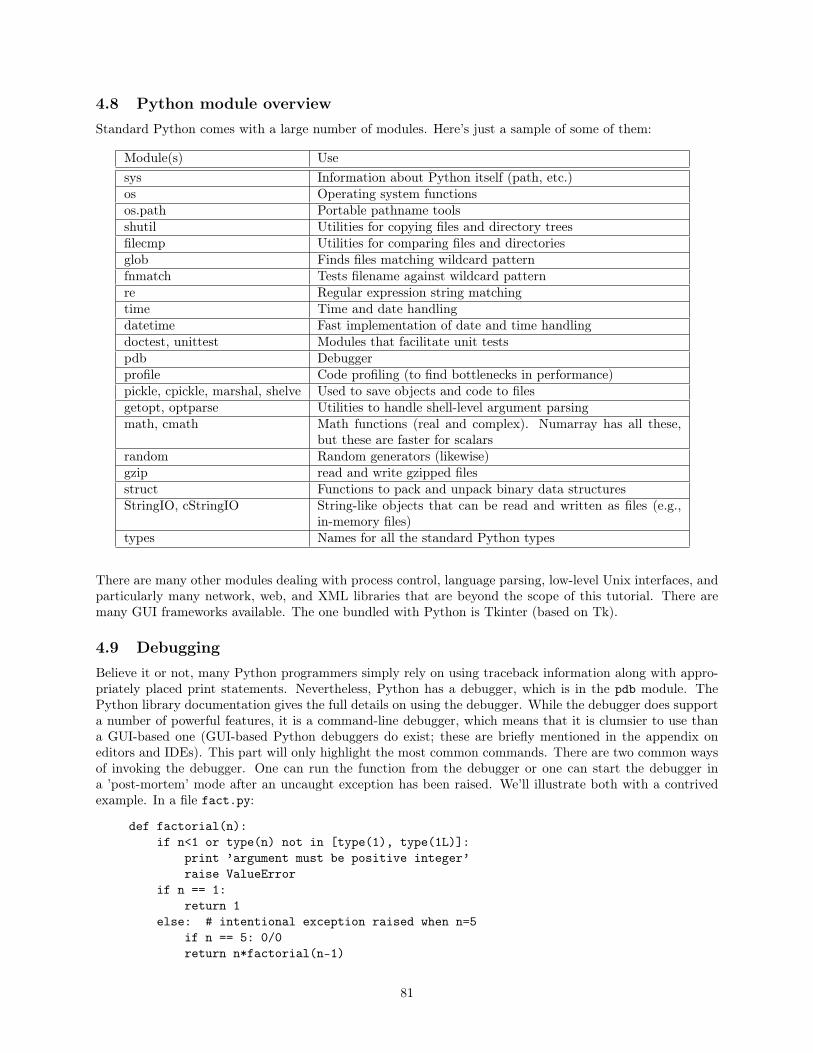
4.8 Python module overviewStandard Python comes with a large number of modules. Here’s just a sample of some of them:

Module(s) Usesys Information about Python itself (path, etc.)os Operating system functionsos.path Portable pathname toolsshutil Utilities for copying files and directory treesfilecmp Utilities for comparing files and directoriesglob Finds files matching wildcard patternfnmatch Tests filename against wildcard patternre Regular expression string matchingtime Time and date handlingdatetime Fast implementation of date and time handlingdoctest, unittest Modules that facilitate unit testspdb Debuggerprofile Code profiling (to find bottlenecks in performance)pickle, cpickle, marshal, shelve Used to save objects and code to filesgetopt, optparse Utilities to handle shell-level argument parsingmath, cmath Math functions (real and complex). Numarray has all these,

but these are faster for scalarsrandom Random generators (likewise)gzip read and write gzipped filesstruct Functions to pack and unpack binary data structuresStringIO, cStringIO String-like objects that can be read and written as files (e.g.,

in-memory files)types Names for all the standard Python types

There are many other modules dealing with process control, language parsing, low-level Unix interfaces, andparticularly many network, web, and XML libraries that are beyond the scope of this tutorial. There aremany GUI frameworks available. The one bundled with Python is Tkinter (based on Tk).

4.9 DebuggingBelieve it or not, many Python programmers simply rely on using traceback information along with appro-priately placed print statements. Nevertheless, Python has a debugger, which is in the pdb module. ThePython library documentation gives the full details on using the debugger. While the debugger does supporta number of powerful features, it is a command-line debugger, which means that it is clumsier to use thana GUI-based one (GUI-based Python debuggers do exist; these are briefly mentioned in the appendix oneditors and IDEs). This part will only highlight the most common commands. There are two common waysof invoking the debugger. One can run the function from the debugger or one can start the debugger ina ’post-mortem’ mode after an uncaught exception has been raised. We’ll illustrate both with a contrivedexample. In a file fact.py:

def factorial(n):if n<1 or type(n) not in [type(1), type(1L)]:

print ’argument must be positive integer’raise ValueError

if n == 1:return 1

else: # intentional exception raised when n=5if n == 5: 0/0return n*factorial(n-1)

81

Note that this is a recursive function, i.e., it calls itself. It has been written to intentionally raise a divide-by-zero exception when the argument is 5 (given the way it is written, that will always happen for values>= 5) . First we show it working:

> > > import fact> > > fact.factorial(4)24

Now let’s try a case that fails, then invoke the postmortem feature:

> > > fact.factorial(7)[...]ZeroDivisionError: integer division or modulo by zero> > > import pdb # the debugging module> > > pdb.pm() # start postmortem debugging> [...] /fact.py(8)factorial()-> if n == 5: 0/0(Pdb)

The debugger now is at the level that started the exception. While in that level you may inspect the contentsof all the variables, move to other levels of the stack, etc. While it is possible to single step and restartexecution, the exception cases generally make those options less useful. Post-mortem mode is mainly forlooking at the state that it failed in rather than executing. The following shows some examples.

(Pdb) p n # print the value of n5(Pdb) w # where in the call stack are we?

<stdin>(1)()[...] /fact.py(9)factorial()

-> return n*factorial(n-1)[...] /fact.py(9)factorial()

-> return n*factorial(n-1)[...] /fact.py(8)factorial()

-> if n == 5: 0/0(Pdb) u # move up one level in the stack> [...] /fact.py(9)factorial()-> return n*factorial(n-1)(Pdb) p n # print the value of n6

The prompt for the debugger is (Pdb). Many of the debugger commands show where it currently is in thecalling stack by printing the name of source file that contains the code (the path is shown as [...] since thatwill be dependent on the location of your code and the function or method that is being executed followedby the source line. Many commands can be invoked with a one or two character abbreviation (the examplemakes use of these abbreviations).

Since this is a recursive function, when it is called with the argument 7, it then calls it self with anargument of 6, then again with 5 and stops there because an exception is raised. That’s why you see therepeated fact.py(x)factorial() references. Three different levels are in the very same function. The toptwo at line 9 and the last at line 8. As we would expect, printing out the value of n where the exceptionoccurs shows it to be 5. The up command (u) moves to the previous call level; the value of n at that levelis 6, as expected. Here are the commands most useful for postmortem examination (parentheses are used toshow the alternate forms of the command, e.g., h or help):

h(elp) [command] list commands, or given specific command, give details of that command

w(here) show stack trace and location of current location

82

d(own) move down in the stack of calls

u(p) move up in the stack of calls

l(ist) [start[, end]] list code. Defaults to 11 lines centered at current location.

p expression print value of expression in the current context

pp expression pretty print value of expression

a(rg) print the current function’s argument list

q(uit) quit the debugger mode

If you are using IPython, you can set it so that it automatically goes into post-mortem mode by startingIPython with the -pdb option, or by typing pdb at the IPython prompt. When it is in this mode it is similarto how IDL behaves when errors occur.

The simplest way of inserting effective breakpoints in the postmortem mode is to place 0/0 where youwish it to stop in your code (presuming nothing will trap that error!).

The function can be run from the start with the debugger. In that mode it is possible to set breakpoints(with options to ignore the breakpoint some specified number of times–useful for stopping after so manyiterations), clear breakpoints, etc. One can also single step through the program, jump to other locations,define aliases, and a standard configuration file. See the Python documentation for a listing of the commands.The following shows a brief example of stepping through the code.

> > > pdb.run(’fact.factorial(7)’)> <string>(1)?()(Pdb) s # start stepping--Call--> [...]/fact.py(1)factorial()-> def factorial(n):(Pdb) # typing <Return> (blank line) executes last command, i.e., s> [...]/fact.py(2)factorial()-> if n < 1 or type(n) not in [type(1), type(1L)]:(Pdb) b factorial # set breakpoint to first statement in functionBreakpoint 1 at [...]/fact.py:2(Pdb) c # continue execution until end or next breakpoint> [...]/fact.py(2)factorial()-> if n < 1 or type(n) not in [type(2), type(1L)]:(Pdb) p n6

4.10 PyRAF4.10.1 Basic features

PyRAF was written here at STScI to replace the IRAF CL, with the goal of allowing the running of IRAFtasks and scripts from a Python environment. IRAF has an extremely rich set of tasks, but using the CLisn’t everyone’s cup of tea. With PyRAF, it is possible to use Python syntax as well as CL syntax, and thisalone greatly enhances the power available to PyRAF users.

The PyRAF tutorial gives a good introduction to using PyRAF, highlighting some of its most importantfeatures:

• Almost all of the CL functionality is available

• CL scripts will run under PyRAF

• Easier debugging of CL scripts

83

• Command-line recall!

• Tab-completion!

• GUI parameter editor

• Powerful graphics system

It is possible to write Python functions that will run under PyRAF using the same parameter passingmechanism as IRAF and the same epar interface.

4.10.2 Using PyRAF

Using Python in PyRAF makes is relatively easy to do complex tasks. For example, MultiDrizzle is writtenalmost entirely in Python (there are some parts that were written in C to improve the execution speed). Togive a useful example, one of the most frustrating aspects of IRAF is that it is very difficult to operate on aset of FITS extensions. Doing

---> imstat *.fits[sci,*]

doesn’t work, and nor does making a file list using files:

---> files *.fits[sci,*] > filelist

But it is relatively easy to make a simple function to do extension processing, returning a list of files withextensions that match a specification. Here’s the code

import pyfitsfrom pyraf import pyrafdef extensions(filespec, ext=None):

”’A module to return a list of files that meet the specification”’filelist = iraf.files(filespec, Stdout=1)outlist = []for exposure in filelist:

thisfile = pyfits.open(exposure)_nextensions = len(thisfile)for i in range(_nextensions)[1:]if(thisfile[i].header[’extname’] == ext.upper():

extver = thisfile[i].header[’extver’]outlist.append(exposure + ’[’ + ext + ’,’ + str(extver) + ’]’)

thisfile.close()return outlist

Since the IRAF files task does wildcard filename processing, it seems a waste not to use it. Note the syntaxof using Stdout=1; this puts the output from the files task into a list which the filelist variable is setto. We use the extensions function by doing:

---> from extensions import *---> extensions(’j*flt.fits’,’SCI’)[’j6me13q9q_flt.fits[SCI,1]’, ’j6me13q9q_flt.fits[SCI,2]’,’j6me13qaq_flt.fits[SCI,1]’, ’j6me13qaq_flt.fits[SCI,2]’,’j95t20hmq_flt.fits[SCI,1]’, ’j95t20hmq_flt.fits[SCI,2]’,’j95t20hoq_flt.fits[SCI,1]’, ’j95t20hoq_flt.fits[SCI,2]’,’j95t20hrq_flt.fits[SCI,1]’, ’j95t20hrq_flt.fits[SCI,2]’,’j95t20huq_flt.fits[SCI,1]’, ’j95t20huq_flt.fits[SCI,2]’,’j95t20hyq_flt.fits[SCI,1]’, ’j95t20hyq_flt.fits[SCI,2]’,’j95t20i1q_flt.fits[SCI,1]’, ’j95t20i1q_flt.fits[SCI,2]’,

84

’j95t20i4q_flt.fits[SCI,1]’, ’j95t20i4q_flt.fits[SCI,2]’,’j95t20i7q_flt.fits[SCI,1]’, ’j95t20i7q_flt.fits[SCI,2]’]---> for extension in extensions(’j*’,’SCI’):... iraf.imstat(extension)[lots of imstat output]

4.10.3 Giving Python functions an IRAF personality

One of the powerful aspects of PyRAF is that it allows you to write Python functions and then wrap them insuch a way that they can be run as though they were IRAF tasks with the same CL syntax that IRAF taskscan be invoked with. The following is an example that uses many of the capabilities that PyRAF provides.In this case, write a short Python function to find the maximum value of an image or images in a fits fileafter smoothing by a boxcar. It needs 3 arguments: the name of the input file, the extension number, andthe size of the boxcar filter.

In a file smax.py:

from numarray.convolve import boxcarimport pyfitsdef smax(input, next, bsize=5):

if next:im = pyfits.getdata(input, next)

else:im = pyfits.getdata(input)

return boxcar(im, (bsize,bsize)).max()

In a separate file smax_iraf.py (though it isn’t necessary; it’s just to keep the IRAF aspects isolated fromthe pure Python functionality.

from pyraf import irafimport smaxdef _smax(image, bsize, max, verbose):

”’Use Python function smax to determine maximum smoothed value”’pos = image.find(’[’) # name contain extension spec?if pos>0:

filename = image[:pos]nextstr = image[pos+1:-1]try: # integer ext or name?

next = int(nextstr)except TypeError:

next = nextstrelse:

filename = imagenext = None

max = smax.smax(filename, next, bsize)if verbose:

print ’smoothed maximum =’, maxiraf.smax.max = max

parfile = iraf.osfn(’home$scripts/smax.par’)t = iraf.IrafTaskFactory(taskname=’smax’, value=parfile, function=_smax)

Finally, create a file named smax.par (in home$scripts, though it can be anywhere you’d like so long asthe reference to that directory in smax_iraf.py is consistent) that contains:

85

input,s,a,""„,"input file (including extension)"bsize,i,a,5„,"size of boxcar to smooth with"max,f,h,0.„,"maximum found"verbose,b,h,yes„,"Print value?"mode,s,h,"al"

Either in PyRAF at the command line or in a CL package script (see PyRAF Programmer’s Guide fordetails)

--> pyexecute(’home$scripts/smax_iraf.py’)

At this point is is possible to use the task like any other IRAF task. You can then:

--> epar smax[...]--> lpar smax

input = pix.fits input file (including extension)bsize = 5 size of boxcar to smooth with(max = 0.) maximum found

(verbose = yes) Print value?(mode = al)

--> smax pix.fits[0] 11 verbose+

The wrapper function _smax is essentially taking the inputs from the IRAF interface and adapting themto the Python function. It is separating the filename into the two components (if there is an extensionspecification). The rest of the smax_iraf.py file is creating an IRAF task object for PyRAF to use bypointing to the parameter file and giving the appropriate name for the task.

If you are particularly fond of working with CL command-style syntax, this a way of accessing Pythonprograms within that environment (or allowing colleagues to do so).

4.11 Final thoughtsWe like Python because it’s possible to be productive very quickly. You can write some ugly quick anddirty code to get what you want done. And then you can throw that code away. If you need to writeproduction code, you can do that too; Python is very robust and full-featured, and chances are there’s amodule somewhere that will help you out.

Exercises1. Write a function to do a regular expression match on FITS header keywords and print all that match

given a filename and regular expression string (see the re module documentation for usage).

2. Wrap the previous function as a PyRAF task.

86

5 What is this object-oriented stuff anyway?The object-oriented features of Python provide capabilities that are hard to obtain by any other means.This tutorial won’t make you a wizard at object-oriented design, nor will it come close to even givingyou a solid grounding, but it will give you a flavor of the advantages that the object-oriented features ofPython provide. The focus will be much more pragmatic than you will normally find in introductions toobject-oriented programming.

5.1 Class basics5.1.1 Class definitions

A class defines its attributes and methods as follows

class Clown:”’Educational Class”’ # docstringdef __init__(self, noise=’Honk Honk’):

self.noise=noisedef makenoise(self):

print self.noise

This creates class called Clown that has one attribute (noise) and one method (makenoise). There are acouple things about this class definition that are not what they seem. First of all, all methods assume thatthe first parameter will be a reference to the object itself. By convention, virtually everyone uses the nameself for that parameter, though Python does not require you to use that name. If you know what’s good foryou, you’ll also use that convention.

So, fair enough, the first argument is a reference to the object. But note that the first argument is notused when calling the method for a given object, Python puts it in for you. This aspect is bound to confuseyou at least a couple times. The example of usage later will illustrate this point.

The second aspect of this class definition that isn’t obvious is the __init__ method. As previouslymentioned, methods with names of the form __xxx__ indicate some sort of indirect effect. The __init__methods is the initialization method. It is what is called when you create an instance of the class. Butnormally you don’t call it directly. For example (in a file clown.py)

> > > import clown> > > bozo = clown.Clown() # create first clown object> > > weepy = clown.Clown(’Boo Hoo’) # create second clown object> > > bozo.makenoise()Honk Honk> > > weepy.makenoise()Boo Hoo

Calling the class as a function in effect calls the __init__ method on a new instance of that class. It is the__init__ method that typically sets up the attributes of the object. Generally the values of the attributesare passed as parameters (but can also be set indirectly or from the general environment; e.g., the currenttime). Since the noise defaulted to ’Honk Honk’, not supplying an argument resulted in the noise attributeset to that value. Also note that Python takes the method call and effectively transforms it into the form ofthe last line of the example; that’s where the value of self gets set. You have to get used to the idea thatthe definition of the method has an extra parameter than the way it will be used.

One point about OO terminology needs to be hammered home. Classes and objects are not the samething. A class defines things about the object, but it should not be confused with those objects. In theprevious example, Clown is the class. The variables bozo and weepy refer to objects created from that class.There is only one class, but many potential objects that can be created from it. The relationship is similar tothat between types of variables and specific variables. In fact, you can think of classes as user-defined typesthat have associated programs (methods) that come along with those types. A common beginner mistake isto be sloppy about the distinction between the two concepts.

87

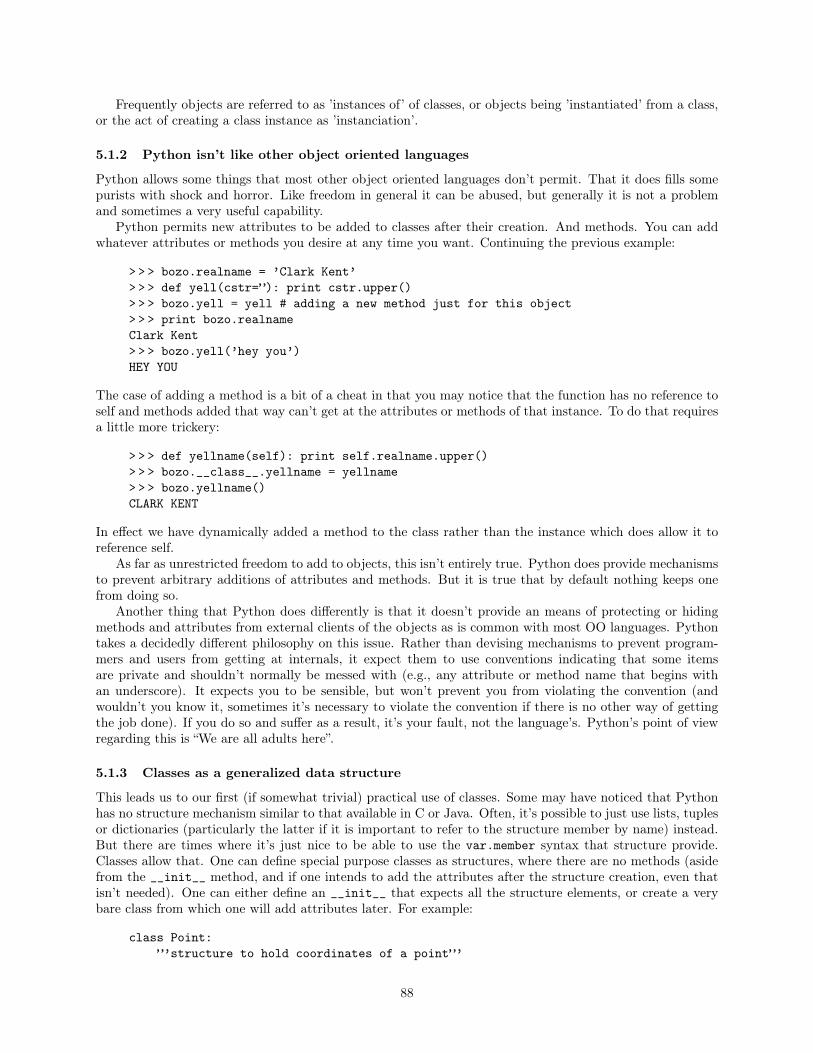
Frequently objects are referred to as ’instances of’ of classes, or objects being ’instantiated’ from a class,or the act of creating a class instance as ’instanciation’.

5.1.2 Python isn’t like other object oriented languages

Python allows some things that most other object oriented languages don’t permit. That it does fills somepurists with shock and horror. Like freedom in general it can be abused, but generally it is not a problemand sometimes a very useful capability.

Python permits new attributes to be added to classes after their creation. And methods. You can addwhatever attributes or methods you desire at any time you want. Continuing the previous example:

> > > bozo.realname = ’Clark Kent’> > > def yell(cstr=”): print cstr.upper()> > > bozo.yell = yell # adding a new method just for this object> > > print bozo.realnameClark Kent> > > bozo.yell(’hey you’)HEY YOU

The case of adding a method is a bit of a cheat in that you may notice that the function has no reference toself and methods added that way can’t get at the attributes or methods of that instance. To do that requiresa little more trickery:

> > > def yellname(self): print self.realname.upper()> > > bozo.__class__.yellname = yellname> > > bozo.yellname()CLARK KENT

In effect we have dynamically added a method to the class rather than the instance which does allow it toreference self.

As far as unrestricted freedom to add to objects, this isn’t entirely true. Python does provide mechanismsto prevent arbitrary additions of attributes and methods. But it is true that by default nothing keeps onefrom doing so.

Another thing that Python does differently is that it doesn’t provide an means of protecting or hidingmethods and attributes from external clients of the objects as is common with most OO languages. Pythontakes a decidedly different philosophy on this issue. Rather than devising mechanisms to prevent program-mers and users from getting at internals, it expect them to use conventions indicating that some itemsare private and shouldn’t normally be messed with (e.g., any attribute or method name that begins withan underscore). It expects you to be sensible, but won’t prevent you from violating the convention (andwouldn’t you know it, sometimes it’s necessary to violate the convention if there is no other way of gettingthe job done). If you do so and suffer as a result, it’s your fault, not the language’s. Python’s point of viewregarding this is “We are all adults here”.

5.1.3 Classes as a generalized data structure

This leads us to our first (if somewhat trivial) practical use of classes. Some may have noticed that Pythonhas no structure mechanism similar to that available in C or Java. Often, it’s possible to just use lists, tuplesor dictionaries (particularly the latter if it is important to refer to the structure member by name) instead.But there are times where it’s just nice to be able to use the var.member syntax that structure provide.Classes allow that. One can define special purpose classes as structures, where there are no methods (asidefrom the __init__ method, and if one intends to add the attributes after the structure creation, even thatisn’t needed). One can either define an __init__ that expects all the structure elements, or create a verybare class from which one will add attributes later. For example:

class Point:”’structure to hold coordinates of a point”’

88

def __init__(self, x, y):self.x = xself.y = y

> > > import point> > > p1 = point.Point(0.,0.)> > > p2 = point.Point(10.3, -22)> > > p2.x10.3> > > p1.y = 100

5.1.4 Those ’magic’ methods

So far we’ve ignored all those strange methods that are of the form __xxx__. What the heck are they for?They are all generally hooks that allow your classes to take advantage of special Python syntax or behaviors.If you’d like to write a class whose objects can be indexed like lists, tuples or dictionaries you can do thatby defining the __getitem__ method for your class. If you define that method suitably, then you take fulladvantage of indexing syntax. The following example will illustrate by defining a class that can collect itemsin a list, but effectively keep them sorted when retrieved by index. It’s not very useful, but it shows how itworks. In file sortedlist.py

class SortedList:def __init__(self):

self.values = []def append(self, value):

self.values.append(value)

def __getitem__(self, index):self.values.sort()return values[index]

def __len__(self):return len(self.values)

> > > import sortedlist as sl> > > x = sl.SortedList()> > > x.append("apple")> > > x.append(3)> > > x.append("pear")> > > x.append(7)> > > x.append("mango")> > > x.append(11)> > > x.append("orange")> > > for v in x: print v3711applemangoorangepear

Nothing requires a class that uses __getitem__ to be finite in the keys that are possible.The magic methods allow one to take advantage of many of Python’s conveniences. The following lists

all the magic methods and the behavior they affect. Note that a number are associated with built-in Pythonfunctions. The first shown (__len__) means that if you define it for your class, than an instance of that

89

class will work with len() (even though the built-in function has no idea of what your class is). These arehooks to allow your class to give the necessary information to many of the standard built-in functions.

Container methods:

__len__(self): What the built-in function len() uses to determine how many elements a class contains.If it isn’t present, len() doesn’t work for that class

__getitem__(self, key): Used when an object is indexed with key (returns self[key]).

__setitem__(self, key, value): Used for assigning to indexed objects (self[key]=value)

__delitem__(self, key): Used to delete self[key].

__iter__(self): Used when next element of an iterator is asked for.

__contains__(self, item): Used for the expression item in self.

Sequence methods:

__getslice__(self, i, j): Returns self[i:j]. In many respects, this method is no longer needed since__getitem__ can handle all slicing (and is necessary if strides are used).

__setslice__(self i, j, sequence): Used for self[i:j]=sequence. Like __getslice__, this methodisn’t really necessary since __setitem__ can handle all slicing cases (including strides).

__delslice__(self, i, j): Used to delete slices.

General methods

__new__(cls...), __metaclass__: for experts only.

__init__(self, ...): You’ve met this one already

__del__(self): called when reference count goes to 0. Usually used when some sort of cleanup is neededthat can’t be expected to be handled by simply deleting all references within the object. Some subtletiesin when this is guaranteed to be called. See documentation.

__repr__(self): called by the built in repr() (also used at interactive prompt) to print info about object

__str__(self): called by the built-in str() to print string representation for object (e.g., print obj)

__lt__,__le__,__eq__,__ne__,__gt__,__ge__: called for <, <=, ==, !=, >, >= operators respectivelywith (self, other) as arguments.

__cmp__(self, other): called by comparison operators if appropriate specific operator magic methodnot defined. Should return negative integer if self<other, 0 if self==other, positive integer ifself>other.

__hash__(self): Used to convert key for dictionary into 32-bit integer. If you don’t know what this means,ignore it for now.

__nonzero__(self): Called when object is used as a truth value. Normally returns False or True.

__unicode__(self): used by built-in unicode()

__call__(self, args...): Called when object is “called” as though it were a function (e.g., IRAF tasksobjects use this trick)

Attribute methods:

__getattr__(self, name): Called when an attribute of the specified name is not found

90

__setattr__(self, name, value): Called when trying to set the value of an attribute. Always calledregardless of whether such an attribute exists (thus a bit tricky to use; see documentation for examples)

__delattr__(self, name): Called when attribute is deleted (e.g., del self.name)

__getattribute__, __get__, __set__, __delete__, __slots__: are powerful and very useful, but arebeyond the scope of this introduction. In particular these allow one to restrict what attributes areallowed for an object, as well as associate functions to be called when getting or setting the value ofthe given attributes. See the documentation for details.

Numeric methods (used to overload numeric operations). The following table shows the magic methodsthat are called when numeric operators or standard functions are called. They all have the samefunction arguments: (self, other). There are three different magic methods for each operator. Toillustrate we’ll use the addition operator as an example. Given your object obj, when Python encountersthe expression obj+3 it sees if you have defined __add__, if so it will call obj.__add__(3). You usethat method to define what should happen when you try to add something to it. You may only acceptnumbers as the “other” argument. Or you may only accept other instances of the same class. It’s up toyou. When Python encounters 3+obj, it will find that ’3’ doesn’t know what to do with obj, it thensees if obj knows what to do, then it calls obj.__radd__(3). The second column refers to when theobject is the rightmost part of a binary operator. The last is when you find “augmented” assignmentstatements. For example: obj += 3 will result in obj.__iadd__(3) being called.

self op. other other op. self self op= other Operator__add__ __radd__ __iadd__ +__sub__ __rsub__ __isub__ -__mul__ __rmul__ __imul__ *__floordiv__ __rfloordiv__ __ifloordiv__ / or //__mod__ __rmod__ __imod__ %__divmod__ __rdivmod__ __idivmod__ divmod()__pow__ __rpow__ __ipow__ **__lshift__ __rlshift__ __ilshift__ < <__rshift__ __rrshift__ __irshift__ > >__and__ __rand__ __iand__ &__xor__ __rxor__ __ixor__ ^__or__ __ror__ __ior__ |__truediv__ __rtruediv__ __itruediv__ /

__coerce__(self, other): Called by numeric operations. Should return a tuple of (self, other) where oneor both have been converted to a common numeric type (see below).

Unary operators:

__neg__(self): -self

__pos__(self): +self

__abs__(self): abs(self) [built-in abs()]

__invert__(self): ~self (bit inversion)

__complex__(self): complex(self) [should return complex value]

__int__(self): int(self) [should return integer value]

__long__(self): long(self) [should return long integer value]

__float__(self): float(self) [should return float]

__oct__(self): oct(self) [should return string]

__hex__(self): hex(self) [should return string]

91

5.1.5 How classes get rich

They inherit, that’s how. Before discussing what they inherit we’ll note that usually by now there is someexplanation of why classes are so wonderful with regard to the theory of object oriented programming. You’dsee terms like abstraction, encapsulation, and polymorphism. These are very nice terms, but we are goingto avoid them for a while. Instead we will take a different track in demonstrating why classes can be useful.One of the other common OO terms is inheritance. What it essentially means is that classes can steal workthat has been done for other classes, particularly if that other class already does an awful lot of what youneed to do, but not exactly. Generally speaking, when you inherit from another class, it is expected thatyou will be able to do all that class can do, and perhaps more. You may not do it the same way, but youwill have all the same public methods and attributes (those that convention has not indicated are to be keptprivate; see 4.7.6). Nothing enforces this though. If you want to be antisocial, you are free to be antisocial.

As usual, examples are the best way of showing what this is all about. Suppose you love dictionariesand want to use them in your program. But for some reason, you only will accept strings as keys, and wantkeys to be case-insensitive. Does this mean you have to rewrite all the machinery for dictionaries? Hardly.Here’s how it can be done with very little code

class SDict(dict):”’Dictionary that only accepts case-insensitive string keys”’def __init__(self, idict = {}):

”’If intializing dict is non-null, examine keys”’keys = idict.keys()values = idict.values()for i in range(len(keys)):

if type(keys[i]) != type(”):raise TypeError

keys[i] = keys[i].lower()dict.__init__(self)for key, value in zip(keys, values):

self[key] = valuedef __getitem__(self, key):

if type(key) != type(”):raise TypeError

return dict.__getitem__(self, key.lower())def __setitem__(self, key, value):

if type(key) != type(”):raise TypeError

dict.__setitem__(self, key.lower(), value)> > > import sdict> > > sd = sdict.SDict({’Bob’:’555-1234’,’Hubble’:’338-4700’})> > > sd{’bob’: ’555-1234’, ’hubble’: ’338-4700’}> > > sd[3]=4[...]TypeError:> > > sd[’BOB’]’555-1234’

Note now that the class name has an argument dict. This is the mechanism to indicate that this class isinheriting from dict, which happens to be the class name associated with standard Python dictionaries.

To really do this right, a few other dict methods should be overridden to handle keys properly. Theseinclude has_key(), update(), get(), and setdefault(). So with about a page of code, you have completelycustomized a powerful data structure for a more specialized use.

One final remark about inheritance. The built-in function isinstance() will return True if the class theobject is being compared to is anywhere in its inheritance hierarchy. For example:

92

> > > isinstance(sd, dict)True

So even though sd is an instance of SDict, it is also considered an instance of every class it inherits from(dict here). This can be used to ensure that any object inherits from a given class (but see the discussionabout duck typing [yes, that’s duck] later, before using this too heavily)

5.2 A more complex example: Representing Source Spectra5.2.1 Goals

This section explores a more realistic problem in more depth. We’ll start with a simpler version of the generalproblem, and do a comparatively simple implementation. Then we’ll discuss how new features can be added,without necessarily doing all the actual work, to illustrate the advantages of the object-oriented approachover a more traditional procedural approach. The example chosen is far from an academic exercise.

The problem to solve is modeling source spectra. Ultimately, we’d like a very general approach thatprovides many features; but we’ll start with more modest goals: we want to be able to build up a sourcespectrum from an unlimited number of analytic source components and be able to sample the net spectrumat whatever wavelengths we choose without using resampling. We’ll address flux integration and tabulatedsource models later. To keep the example short, we’ll only implement two analytic models: Gaussian linesand black bodies (adding others is straightforward). We’ll also assume that wavelengths are always inangstroms and the source spectra are in units of Fλ.

5.2.2 Initial Implementation

The approach taken for the models may strike many as unusual, but it allows great flexibility. We’ll show thesource code for the basic implementation, and then go into a lot of detail explaining how it works. It probablywill appear unintelligible at first glance even though it is relatively short. Have patience. This example makesuse of inheritance and abstract classes. The latter is an important and often used technique. Abstract classesare generally incomplete implementations that are never expected to have an instance created of it directly.They are intended to be inherited by other classes that will fill out the functionality. Classes that will haveinstances created are sometimes called concrete classes in contrast to abstract.

import numarray as n

class SourceFunction:”’Abstract Class representing a source as a function of wavelength

Units are assumed to be Flambda”’

def __add__(self, other):return CompositeSourceFunction(self, other, ’add’)# __radd__ not needed

class CompositeSourceFunction(SourceFunction):”’Source function that is a binary composition of two other functions

”’def __init__(self, source1, source2, operation):

self.comp1 = source1self.comp2 = source2self.operation = operation

def __call__(self, wave):if self.operation == ’add’:

return self.comp1(wave) + self.comp2(wave)

93

class BlackBody(SourceFunction):def __init__(self, temperature):

self.temperature=temperaturedef __call__(self, wave):

BBCONST =6.625e-34 * 3e8/(1.38e-23 * 1.e-10)exparg = BBCONST/(n.array(wave)*self.temperature)exparg[exparg>600] = 600. # to prevent overflowsreturn 1.e21/(wave**5 * (n.exp(exparg)-1.))

class Gaussian(SourceFunction):def __init__(self, center, width):

self.width=widthself.center=center

def __call__(self, wave):return n.exp(-(wave-self.center)**2/(2*self.width**2))

Before explaining how it works, we’ll give some context by showing how it is used.

> > > import spec as s> > > from pylab import *> > > spectrum = s.BlackBody(6000) + s.Gaussian(3000, 50)> > > wavelengths = arange(7000) + 1.> > > plot(spectrum(wavelengths))

0 1 0 0 0 2 0 0 0 3 0 0 0 4 0 0 0 5 0 0 0 6 0 0 0 7 0 0 000 . 5 11 . 522 . 53

A composite spectrum is built simply by adding basic elements together as an expression (one could addmore Gaussian components at different wavelengths and widths just by adding more terms in the expression).

94

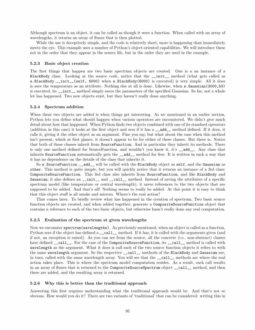
Although spectrum is an object, it can be called as though it were a function. When called with an array ofwavelengths, it returns an array of fluxes that is then plotted.

While the use is deceptively simple, and the code is relatively short, more is happening than immediatelymeets the eye. This example uses a number of Python’s object-oriented capabilities. We will introduce thesenot in the order that they appear in the source file, but in the order they are used in the example.

5.2.3 Basic object creation

The first things that happen are two basic spectrum objects are created. One is a an instance of aBlackBody class. Looking at the source code, notice that the __init__ method (what gets called ass.BlackBody.__init__(self, 6000) when s.BlackBody(6000) is executed) is very simple. All it doesis save the temperature as an attribute. Nothing else at all is done. Likewise, when s.Gaussian(3000,50)is executed, its __init__ method simply saves the parameters of the specified Gaussian. So far, not a wholelot has happened. Two new objects exist, but they haven’t really done anything.

5.2.4 Spectrum addition

When these two objects are added is when things get interesting. As we mentioned in an earlier section,Python lets you define what should happen when various operators are encountered. We didn’t give muchdetail about how that happened. When Python finds two objects combined with one of its standard operators(addition in this case) it looks at the first object and sees if it has a __add__ method defined. If it does, itcalls it, giving it the other object as an argument. Fine you say, but what about the case when this methodisn’t present, which at first glance, it doesn’t appear to be for either of these classes. But there is. Noticethat both of these classes inherit from SourceFunction. And in particular they inherit its methods. Thereis only one method defined for SourceFunction, and wouldn’t you know it, it’s __add__. Any class thatinherits SourceFunction automatically gets the __add__ method for free. It is written in such a way thatit has no dependence on the details of the class that inherits it.

So s.SourceFunction.__add__ will be called with the BlackBody object as self, and the Gaussian asother. This method is quite simple, but you will quickly notice that it returns an instance of a 3rd class:CompositeSourceFunction. This 3rd class also inherits from SourceFunction, and like BlackBody andGaussian, it also defines an __init__ and __call__ method. Instead of saving the attributes of a specificspectrum model (like temperature or central wavelength), it saves references to the two objects that aresupposed to be added. And that’s all! Nothing seems to really be added. At this point it is easy to thinkthat this object stuff is all smoke and mirrors. Where’s the real action?

That comes later. To briefly review what has happened in the creation of spectrum, Two basic sourcefunction objects are created, and when added together, generate a CompositeSourceFunction object thatcontains a reference to each of the two basic objects, but otherwise hasn’t really done any real computation.

5.2.5 Evaluation of the spectrum at given wavelengths

Now we encounter spectrum(wavelengths). As previously mentioned, when an object is called as a function,Python sees if the object has defined a __call__ method. If it has, it is called with the arguments given (andif not, an exception is raised). As you can see from the source, all the concrete (i.e., non-abstract) classeshave defined __call__. For the case of the CompositeSourceFunction, its __call__ method is called withwavelength as the argument. What it does is call each of the two source function objects it refers to withthe same wavelength argument. So the respective __call__ methods of the BlackBody and Gaussian are,in turn, called with the same wavelength array. You will see that the __call__ methods are where the realaction takes place. This is where the spectrum model computation resides. As a result, each call resultsin an array of fluxes that is returned to the CompositeSourceSpectrum object __call__ method, and thenthese are added, and the resulting array is returned.

5.2.6 Why this is better than the traditional approach

Answering this first requires understanding what the traditional approach would be. And that’s not soobvious. How would you do it? There are two variants of ’traditional’ that can be considered: writing this in

95

a language like C or Fortran, or writing it in IDL using arrays. Let’s take these in turn. With the exampleabove, we can construct a composite spectrum from any number of basic elements by adding them together.So the traditional C/Fortran approach must be able to deal with an unlimited number of components ofmany types. That may not seem so hard, just provide a list somehow. Yes, that works for this basicversion. But the example above hasn’t yet addressed multiplicative factors, which are easy to address in thisframework (and a later version will show that). Thus the software will have to deal with arbitrarily complexexpressions of spectral components. It is hard to escape the fact that one needs to write an expression parser(as synphot does). That is no simple matter at all. For the Python object-oriented approach, it is completelyunnecessary since Python is doing the parsing for you. This alone is a huge advantage.

Is this an advantage over IDL as well? That depends on how you approach the problem. If the approachis to take advantage of the array capabilities, one might consider generating an array for each componentat a specified set of wavelengths. If one can do this for all components using the same set of wavelengths,then IDL can handle combinations of spectra using its array expression facilities. Parsing expressions wouldnot be necessary. But this approach is fraught with difficulties. What wavelengths to choose? If you don’tchoose a set that is fine enough, you risk missing important features in the components. What if someonechooses a Gaussian line width of 0.01 angstroms and you only sample every angstrom? No matter what yourdefault choice, eventually someone will find it a problem. What range of wavelengths should you cover? Thatinvolves choices as well. Arbitrary restrictions will come back to bite you eventually. When someone asksfor fluxes for a specific wavelength set, how do you get these from the sampled wavelengths? Interpolation?What kind of interpolation? Choices there can often backfire (suppose it generates negative values whenthe spectrum component model was always positive). When the spectrum model can use tabular spectrain addition to analytic spectra, will the resampling of the tabular spectra onto a standard wavelength setintroduce unacceptable errors, particularly in view of the fact that there may be subsequent resamplings?

In fact, the use of arrays to represent all components is a possible choice for C or Fortran implementationsas well, and the same issues arise there also. Indeed, that’s how synphot was implemented. And every oneof the concerns listed have been manifested as actual problems in practical usage of synphot at one time oranother. There has never been a truly satisfactory solution to them using standard wavelength sets.

We’ll detail other advantages of object-oriented approach after adding some more features and capabilities.

5.2.7 Take 2: handling multiplicative effects

Simply adding fixed components together isn’t very useful. There must be a way of handling scaling eachcomponent as well as handing effects that are multiplicative such as absorption lines or reddening. This nextversion adds these capabilities (new or modified code is shown prefaced with |).

import numarray as n

| class TransmissionFunction:| ”’Abstract Class representing a transmission function of wavelength|| Unitless”’| def __mul__(self, other):| if isinstance(other, TransmissionFunction):| return CompositeTransmissionFunction(self, other)| if isinstance(other, SourceFunction):| return CompositeSourceFunction(self, other, ’multiply’)| if type(other) in [type(1), type(1.)]:| return CompositeTransmissionFunction(| self, ConstTransmission(other))| else:| print "must be product of TransmissionFunction, SourceFunction or constant"| def __rmul__(self, other):| return self.__mul__(other)|| class CompositeTransmissionFunction(TransmissionFunction):

96

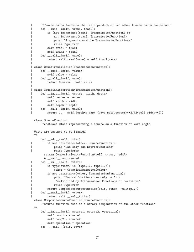
| ”’Transmission function that is a product of two other transmission functions”’| def __init__(self, tran1, tran2):| if (not isinstance(tran1, TransmissionFunction) or| not isinstance(tran2, TransmissionFunction)):| print "Arguments must be TransmissionFunctions"| raise TypeError| self.tran1 = tran1| self.tran2 = tran2| def __call__(self, wave):| return self.tran1(wave) * self.tran2(wave)|| class ConstTransmission(TransmissionFunction):| def __init__(self, value):| self.value = value| def __call__(self, wave):| return 0.*wave + self.value|| class GaussianAbsorption(TransmissionFunction):| def __init__(self, center, width, depth):| self.center = center| self.width = width| self.depth = depth| def __call__(self, wave):| return 1. - self.depth*n.exp(-(wave-self.center)**2/(2*self.width**2))

class SourceFunction:”’Abstract Class representing a source as a function of wavelength

Units are assumed to be Flambda”’

def __add__(self, other):| if not isinstance(other, SourceFunction):| print "Can only add SourceFunctions"| raise TypeError

return CompositeSourceFunction(self, other, ’add’)# __radd__ not needed

| def __mul__(self, other):| if type(other) in [type(1), type(1.)]:| other = ConstTransmission(other)| if not isinstance(other, TransmissionFunction):| print ’Source functions can only be ’+ \| ’multiplied by Transmission Functions or constants’| raise TypeError| return CompositeSourceFunction(self, other, ’multiply’)| def __rmul__(self, other):| return self.__mul__(other)

class CompositeSourceFunction(SourceFunction):”’Source function that is a binary composition of two other functions

”’def __init__(self, source1, source2, operation):

self.comp1 = source1self.comp2 = source2self.operation = operation

def __call__(self, wave):

97

if self.operation == ’add’:return self.comp1(wave) + self.comp2(wave)

if self.operation == ’multiply’:return self.comp1(wave) * self.comp2(wave)

class BlackBody(SourceFunction):def __init__(self, temperature):

”’Temperature in degrees Kelvin”’self.temperature=temperature

def __call__(self, wave):BBCONST =6.625e-34 * 3e8/(1.38e-23 * 1.e-10)exparg = BBCONST/(n.array(wave)*self.temperature)exparg[exparg>600] = 600. # to prevent overflowsreturn 1.e21/(wave**5 * (n.exp(exparg)-1.))

class Gaussian(SourceFunction):def __init__(self, center, width):

self.width=widthself.center=center

def __call__(self, wave):return n.exp(-(wave-self.center)**2/(2*self.width**2))

Again, we will start with an example of usage:

> > >> > > spectrum = s.GaussianAbsorption(4000,20,0.8) * \... (s.Gaussian(3000,100)+2.*s.BlackBody(6000))> > > plot(spectrum(wavelengths))

98

0 1 0 0 0 2 0 0 0 3 0 0 0 4 0 0 0 5 0 0 0 6 0 0 0 7 0 0 00 12 34 56

No really new object-oriented concepts are introduced in this example except perhaps the checking ofobject types. This is primarily an extension of the previous concepts to new operations and classes. Againit is useful to trace what happens for the usage example.

Three objects are initially created, two of them essentially identical to the previous example (thoughthey have richer operator behavior now). The third is an instance of a new kind of wavelength function:GaussianAbsorption which is a concrete case of a general TransmissionFunction. The key thing to noteis that these two kinds of functions have somewhat different rules about what can be done with them.Transmission functions are unitless. They can be multiplied with either transmission or source functions.But they cannot be added with each other (or anything else for that matter). Source functions have specificunits. Thus they can be added with other source functions or multiplied by unitless functions, producinga new source function in the process. These rules are embodied in the definitions (or lack of them) for theoperator methods for these classes. We’ll get back to the details of these after following the example throughto the end.

The first difference that shows up is when the BlackBody object is multiplied by a floating point constant.Since floating point constants don’t know what to do with SourceFunction objects, it tells Python it can’tdeal with it which causes Python to then look to see if the SourceFunction object has a __rmul__ method.It does, so it is called with the floating point value as its argument. Since multiplication is symmetric forthis case, all that method does is call the __mul__ method (don’t duplicate code if you don’t need to!). Thatmethod checks to see if the type of the other object is either a TransmissionFunction instance, an integeror float value (if none of these, it gives up). If it is a numeric constant, it turns it into a ConstTransmissionobject and then proceeds to create a composite source function (which now has been modified to acceptboth kinds of objects and to support addition and multiplication by saving the operation type as one of theobject’s attributes).

99

The resulting composite source function is added to the GaussianSource object the way it was before(but now it is necessary to indicate addition in the new composite source object (which has as one ofit elements another composite source object). Finally this is multiplied by a Gaussian line absorptiontransmission function creating a third composite source object. In this case it is the GaussianAbsorptionobject’s __mul__ method that is called first. That returns the final composite source function object.

As in the previous case, calling the final object with a wavelength array is what evaluates the model byevaluating the components of each composite object in turn and then adding or multiplying the results asappropriate and returning those back in turn (notice that the __call__ method for the composite sourceobject checks to see which operation to perform).

5.3 Further enhancements to the spectrum modelAt this point we’ll stop presenting full implementations and instead discuss how one might go about enhancingthe capabilities of code (we have only so much space and you have only so much patience). Each issue willshow one or more examples of usage for the proposed mechanism.

5.3.1 Determining total flux

Very often the point of making such spectral source models is being able to determine the total flux expected.After all, imaging observations effectively integrate flux density over wavelengths, and one often wants tocompare the observations with a model. Integrating the flux density of a model spectrum is an essentialcapability.

Fortunately, numerical integration is a well-studied subject. Unfortunately, no general algorithm isfoolproof for all functions that must be integrated. The advantage of the approach chosen for modelingspectra is that it provides a means for avoiding these problems. Generally speaking, the problem withnumerical integration is knowing where the function is changing rapidly. Since each source and transmissionfunction is specially constructed, we can include as part of their behaviors (i.e., methods) a means of themtelling us where we should sample the function for integration purposes. In other words we could define amethod (with a specific implementation for each kind of function) called waveset() that returns an arrayof wavelengths that properly sample the structure of the function. For example, for the GaussianSource orGaussianAbsorption objects, it would ensure that it returned enough points within the main part of theGaussian profile. It possibly could take an optional parameter that indicated sampling frequency or whatamount of percent change was permitted in the function between samples. The integration routine woulduse these wavelengths to evaluate the function for integration purposes.

But what about composite objects? What are their wavelength sets? Simple, when one calls .waveset()for a composite object, it calls .waveset() on the two components and joins them (i.e., the union of thereturned wavelengths. If either of those objects are composite, the same process is repeated until it hitsendpoint spectrum objects (just like addition).

The integration routine would be defined in the abstract class (it should have no dependencies on thespecific functions) and would first call the .waveset() method to get the wavelengths it will use for doingthe numerical integration. Possibly several integration methods could be used, either as options to the mainmethod or as different methods. In this way, it should be possible to make the integration relatively robustagainst a wide variety of model parameters.

An example of use:

> > > source = GaussianAbsorption(4000,20,0.8) * \... (Gaussian(3000,100) + 1.e10*BlackBody(6000))> > > source.integrate() # returns integrated flux

5.3.2 Handling empirical spectra

A means of modeling spectra that could not accept empirical spectra would be very limited. The examplegiven only addressed analytical models. How could one combine the two approaches? If one grants that it willbe necessary to resample the empirical spectra (and it is–e.g., combining it with a very narrow line analyticalfeature that is smaller than the spacing in the empirical model), then one may treat the empirical spectra

100

as an extreme form of analytical spectra. The interpolation behavior is then embodied in the evaluationbehavior (i.e., the __call__ method). The initialization of the SourceFunction object saves the arrays thatdefine the wavelengths for the fluxes and the fluxes themselves. Likewise, the .waveset() method returnsthe specific wavelengths for the fluxes used. Constructed that way, empirical spectra fit very well within thisobject framework. Likewise, empirical transmission functions can be handled the same way.

An example:

> > > data = pyfits.getdata(’fuse.fits’)> > > source = TableSource(flux=data.field(’flux’),... wavelength=data.field(’wave’))

5.3.3 Valid wavelength ranges

In many instances, particularly with empirical data, it may be necessary to indicate what the valid wavelengthrange of the component and the net spectrum model is. This is fairly easy to add. Each component mayadd as part of its initialization what the valid range is for that component (even for analytical models) asan optional parameter. Empirical components would, by default, take their valid range from the range ofwavelengths for the flux values. The net valid range would be obtained from a method called waverange(),defined for the base class to use the values saved for basic components, and it would be overridden forcomposite objects to call waverange() for each of its components and take the intersection of those rangesto obtain the net range for that composite. A value of None at either end would mean no limit. For example,using the previous table data and a black body:

> > > source.waverange()[985., 1085.]> > > BlackBody(6000).waverange()[None, None]

It may also make sense to provide a method to greatest extents of ranges present (the union of all ranges).A secondary use of wavelength ranges is to bound integration of analytic components that no intrinsic

limits to their range. For example, if the net range of a given model is unbounded, then a default range maybe used or an exception may be generated.

5.3.4 Component normalization

Frequently it is necessary to define the scaling factor for a given component based on the integrated flux ofthat component, often through a different transmission function than being used in the given model (saya V filter). One way to incorporate this capability into the proposed scheme is to add a scale factor to allfunction objects (including composite objects) that defaults to 1.0. Then a .normalize() method wouldbe added to the base class which takes one mandatory argument (the integrated flux expected) and anoptional transmission function (.e.g., a filter transmission curve) to be applied to the source function beforeintegration. Since this is generic to all source functions there need be only one version defined for the baseclass. This method then does the integration on the net source function, and takes the ratio of the integrationresult with the desired value to set the scale factor. The scale factor must of course be used by the __call__method to apply it to the computed fluxes. Some examples (units are addressed later):

> > > source = BlackBody(6000).normalize(VMag(23.3))> > > source = (Gaussian(3000,50) +... 1.e10*BlackBody(6000)).normalize(Jy(3.1),... trans=JohnsonV)

5.3.5 Redshifts

Handling redshifts is straightforward as well. Any function component (source or transmission) can take anoptional z parameter at initialization and save it as an attribute. This works for concrete components butnot so conveniently for composite ones. These can be handled either by defining a method to set the z for

101

the composite object, or a function that does the equivalent. The effect of a nonzero z is to transform theintrinsic wavelengths being used and divide Fλ by (1+z ). The flux is computed at the ’rest’ wavelength for themodel. Thus all methods that deal with wavelengths (__call__, waverange, waveset, etc.) need to applythe appropriate transformation to the wavelengths. For example, in the __call__ method, the wavelengthsgiven as an argument would be redshifted to the source’s rest frame, and then the model applied to thatset of wavelengths and the resulting fluxes returned. For things that return wavelengths apply the inversetransformation. Both these transformations can be handled as standard functions used by all the relevantroutines. In fact, it is likely that a common interface routine for all these methods can be defined for thebase classes that then call the component-specific version that doesn’t worry about z at all. This isolatesthe redshift handling code to a small number of locations. The following snippets of code illustrate how thiswould be accomplished.

class SourceFunction:[...]

def __call__(self, wavelengths):return self.resteval(invZ(wavelengths, self.z))/(1.+self.z)

def waveset(self):return Z(self.restwaveset(), self.z)

What had previously been defined as __call__ and waveset in the concrete function classes now are renamedresteval and restwaveset respectively. Since validrange is only defined for the base class, there is littlereason to depend on such indirection.

The following shows how redshift would be used.

> > > source = BlackBody(6000,z=1.3) # or> > > source = BlackBody(6000).z(1.3)> > > source = (Gaussian(3000,20)+Blackbody(6000)).z(1.3) # or> > > source = Z(Gaussian(3000,20)+Blackbody(6000), 1.3)> > > source = (GaussianAbsorption(3000,20,0.8,z=.3)* \

BlackBody(6000,.5)).z(.8)

The last case shows two components with individual redshifts and then with a subsequent redshift appliedto the combination (cumulatively). Note that it is possible to define a function Z that actually performsa transformation of wavelengths when given a scalar or array, and sets the z attribute of source functionswhen those appear as arguments. Not everyone may think that it would be good to share the same functionfor both uses.

5.3.6 Different unit systems

Any practical modeling system would have to handle many different units, both for the wavelengths, andthe fluxes. The approach taken here is to use only one for internal representation (a common approach)and deal with other units only for conversion to and from other representations. At first glance unitsappear deceptively simple, but unfortunately, they are anything but. This is partly because there is contextinvolved (e.g., electron volts can be interpreted as wavelengths or energies), and because there may bedependencies on other values such as exists betweenFλ and Fν (depends on the wavelengths or frequenciesused). The first problem can be solved by confining our context to spectra (electron volts is presumed tobe a wavelength). The second is trickier since it needs more than the flux to transform. It would be niceto have transformation functions that only took scalar or arrays as arguments and applied the appropriatescaling factor to generate the values in the appropriate units. It usually is important to have things likeunit transformations have a consistent interface so that one does not need a lot of code checking whetherthe conversion function is this type or that before applying it. So a pragmatic solution is to just allow for anoptional wavelength argument to the unit conversion functions that is mandatory for conversions betweenfrequency and wavelength representations. Allowing the specification of the units for the __call__ methodavoids having to again specify the wavelength in the unit conversion function since the wavelength is alreadypresent as a argument. Dealing with this problem is not necessary for wavelength unit conversions. Forexample:

102

> > > asJy(BlackBody(6000)(NM(300)) # evaluate at 300 nm, return in Janskys> > > source = GaussianSource(EV(.5), EV(.1)) # centered at .5 electron volts> > > source(NM(10), funits=Fnu) # or> > > asFnu(source(NM(10), NM(10))

5.4 The upside to object-oriented programsA major goal of Object-Oriented Languages is achieving as much decoupling of dependencies as possible.The more one can isolate code dependencies and make it more modular, the fewer problems you will generallyhave when changes are needed. When you must make changes in many places to add a new feature, you aremuch more likely to break something. Having to deal with many modules and locations at once makes itdifficult to really understand what is going on; it is far easier to get confused.

This is done by trying bring the code that manipulates data as close to the data as possible. A mindsetthat is focused on functions primarily (as C and Fortran are) forces one to do a lot of bookkeeping to keeptrack of the data. Where is it? What things can I do with it? Typically it leads to lots of conditional codethat says if it is this kind of data do this, if that, do that, and so forth. Add a new kind of data or variant,and you must go and change many functions so that they can deal with it. Very Bad.

With objects, the code is kept with the object. Each object knows how to do what’s required of it. Thesemay vary from object to object or may not. To add a new object that is supposed to ’play nicely’ withothers, usually doesn’t require making changes to the code of all the others. Often it doesn’t require any.

The spectrum model example is a good illustration of that. To add a new model doesn’t require handlingintegration, units, redshift, or many other common effects. Most of the code for the model is that focused onwhat the model is all about: determining the flux at a given wavelength. And that’s primarily it. Secondarilyit is giving hints about where the model changes the most. And very little else. The cost to add models isabout as minimal as it could be. Likewise, the general algorithms such as that doing the composite evaluationor integration, don’t need to know anything about the specifics of any of the models. This is generally aGood Thing. (This is referred to as ’data hiding’ or ’encapsulation’ in the OO biz.)

Despite the simplicity of the model code, it is quite capable of generating quite complex networks ofsources and transmission functions. The simplicity of organization does not prevent it from being used forcomplex cases. Given the operator overloading features (something not available in Java), it is possibleto make these networks correspond very closely to their mathematical equivalent. Unlike synphot, it isn’tnecessary to form an expression as a string and write a program to parse and evaluate it. The code is thedefinition! (Lest those who say that this is bad, Python makes it trivial to evaluate strings containing suchcode, so it’s just as easy to do it the other way).

Much of the power of Object-Oriented Programming comes from what is called ’polymorphism’. Whatit means is having several objects that share some common behavior and attributes, but possibly have muchthat is different as well. The spectral components example very much makes use of this. They all must beable to evaluate themselves at requested wavelengths (how they do so is entirely up to them). They mustgive a set of wavelengths that sample them well. They must handle redshifts, normalization, and integration.They must support basic addition and multiplication. Some of these behaviors are handled by the parentclass, some by the child classes. But they all must meet these standard behaviors. They may have othernonstandard methods and attributes. There is nothing wrong with that. But the point is that it allows oneto write very general software that takes a wide variety of components and handles them uniformly. Theyhandle their specific differences internally.

If you find you are writing a lot of functional code that has many tests for the kind of data it is workingon, particularly the same set of tests in different functions, that is usually a sign that the problem is a goodcandidate for polymorphic objects.

Notice that most of the enhancements did not require a great reworking of the architecture. Given aproperly designed framework, quite powerful enhancements are possible without extensive reworking.

The nice thing about Python is that it doesn’t force you to put everything in an object-oriented framework.You can make it entirely functional or a hybrid. A good example of a hybrid approach is numarray wheremany operations are handled by functions, not methods, primarily since it is a better match to mathematicalconvention.

103

5.5 The downsideInvariably there is some bad with the good. Object-oriented technology has its downside. One is thatalthough it is very good at reducing dependencies, the manner in how that is done can make it more difficultto follow what actually is happening as time progresses. This can make debugging more involved if there aremany objects involved, and many jumps from one object to another. Those used to procedural programming(which by its nature is more time-oriented) can find this more frustrating to understand. Taking thisspecific example, one sees the flow of program control jump from child class to parent and back, and fromone object’s method to another that it refers to. The flow is just not as linear through the file as manyprocedural programs would be.

This is partly because objects rely heavily on indirection, either through the objects they link to, or theclasses they inherit from. Indirection is an indication of greater abstraction, more power, and a correspond-ingly greater power to confuse.

Some problems don’t lend themselves to object orientation. The example does, but there are cases thatare hard to frame this way. It is a mistake to try to force all problems into one approach.

Those that are experienced at procedural programming tend to have a harder adjustment to an object-oriented approach. It’s quite easy to fall into a pattern of using classes in a mostly procedural way. Thebest guard against that is by reading good examples of OO design (in real projects) or have others that havethat kind of experience review your code.

The previous section glibly asserted that example showed how flexible the OO architecture was given aproper framework. Achieving the proper framework is often not trivial. The ability to do so comes withexperience and some analysis of the problem. Typically, OO design puts more emphasis on the analysis anddesign phase than does a procedural approach. A good design makes it easy to extend and maintain, a baddesign not. The same certainly can be said for any approach (including procedural), but an OO approachis more sensitive to the quality of the design. Having said that, Python is so productive that one shouldparticularly avoid becoming paralyzed by the analysis and design phase. Experimentation is an importantpart of the design process and Python makes that comparatively easy. Do not make the mistake of tryingto figure everything out before starting. Think a little, try something, start over.

5.6 Loose endsTaking a case study approach to OO programming in Python means some mechanical details have beenpassed over. It’s not possible to cover them all, but some of the basics will be elaborated.

5.6.1 Method inheritance and overloading

When you use a method for an object Python will search for the method definition up the inheritance chain.It sees if the method exists for the specific class that is being used. If it doesn’t exist there, it looks at theclass that it inherits from to see if that class defines it. If not and that class inherited from yet another,that one will be searched for the method until there are no further inherited classes (then an exception israised). Overloading a method means that it exists in an inherited class and it is redefined in a descendantclass. Generally speaking, overloading a method means that the method should support the same argumentinterface that the original method does (nothing enforces that), though it usually is considered permissibleto allow extra optional arguments and keywords.

5.6.2 Object initialization

One thing to realize is that, unlike some other OO languages, Python requires fairly explicit instructionsregarding objects. One such area is in their creation. All classes have an implicit default definition of__init__ that exists if they do not define one. So it is not necessary to define __init__ (even if inheritanceis not used). But realize that no attributes can be created at initialization if __init__ is not defined sincethat is where they must be set (it is always possible to add them any time later if you don’t use specialfeatures to prohibit them). If you inherit from a class that does define its own __init__ and you don’t define__init__ in the subclass, then the original __init__ will be used. If you wish to define a new __init__for the subclass and invoke the parent class __init__ you must do so explicitly (as shown in the example in

104

section 5.1.5). Or you may completely ignore the parent class __init__ if you are replacing its functionalityentirely. You have full control, but you must be explicit about what initializations you wish to be done.

5.6.3 Multiple inheritance

Python permits classes to inherit from more than one class. When these parent classes share the samemethod names, Python has clear (but involved) rules about determining the search order for which one ituses (called “method resolution order”). It is considered good practice to use multiple inheritance as sparinglyas possible. See http://www.python.org/2.3/mro.html.

5.6.4 New-style vs old-style classes

With version 2.2 Python introduced “new-style” classes that provided many more capabilities for classes. Formost beginners, these distinctions are not relevant since they involve fairly advanced concepts. All Pythondata types are now “new-style” classes. Old-style classes were retained for compatibility purposes. If yourclass definition does not inherit from “object” or a built-in Python data type (lists, strings, etc.) it is anold-style class, otherwise it is a new style class. Again, you are not likely to need to know or care yet; thisexplanation is to explain why you may see these two variants:

class Class: # old styleclass Class(object): # new style

When Python 3.0 shows up, it will only support new style classes and then inheriting from object will beoptional. (ref. http://www.python.org/2.2.2/descrintro.html)

5.6.5 Duck typing

Making use of polymorphism does not require that the objects inherit from a common class. It is a commonidiom in Python to allow objects that may have no common parent to be used in the same context so longas they support the needed behaviors. For example, there are many things that expect a ’file-like’ object.Something that can be written to and read from as though it were a file. So long as you provide an objectthat has the needed methods and attributes, that’s good enough. Likewise, when writing your own classesand code, be careful not to try to be too specific on the types of arguments. It is usually better to encloseattempts to use them in try/except blocks rather than enforce that they be a certain type or class. In thisway the code will be much more flexible.

And the phrase “Duck typing”? It derives from the philosophy that if something quacks like a duck, walkslike a duck, looks like a duck, etc., as far as you are concerned, it is a duck. It doesn’t actually have to beof type “Duck” for it to be acceptable. Use of this phrase indicates that this approach is being used.

5.7 What you haven’t learned about Python (so if you are interested, go lookit up)

5.7.1 iterators

Iterators are a powerful extension to the language. They are objects that can be iterated over in that onecan ask for the next item until the end is reached. They are like sequences in some respects but cannot beindexed arbitrarily. They can be infinite. Many things in Python that used to return lists now are iterators.Iterators can be used in for statements.See http://www-106.ibm.com/developerworks/library/l-pycon.html?n-l-9271.

5.7.2 generators

Generators are similar to iterators except they allow one to write functions that repeatedly return valuesand retain the state of where they last left off.See http://www-128.ibm.com/developerworks/linux/library/l-pycon.html.

105

5.7.3 list comprehensions

These are a convenient way of creating lists. An example explains best:

> > > newlist = [i**2 for i in range(10)]

creates a list of all squares of 0 through 9.See http://www.secnetix.de/~olli/Python/list_comprehensions.hawk for the full details.

5.7.4 sets

Python has recently introduced a set data type (otherwise known as unordered collections).See http://www.python.org/doc/2.4/whatsnew/node2.html.

5.7.5 metaclasses

New-style classes provide some very powerful capabilities, particularly with regard to ’metaclass’ capabilities.These generally are quite advanced aspects, considered ’brain-exploding’ by many.See http://www.python.org/2.2.2/descrintro.html#metaclass if you are fearless.

5.8 The Zen of Python(author: Tim Peters, a Python legend)

• Beautiful is better than ugly.

• Explicit is better than implicit.

• Simple is better than complex.

• Complex is better than complicated.

• Flat is better than nested.

• Sparse is better than dense.

• Readability counts.

• Special cases aren’t special enough to break the rules.

• Although practicality beats purity.

• Errors should never pass silently.

• Unless explicitly silenced.

• In the face of ambiguity, refuse the temptation to guess.

• There should be one– and preferably only one –obvious way to do it.

• Although that way may not be obvious at first unless you’re Dutch.

• Now is better than never.

• Although never is often better than *right* now.

• If the implementation is hard to explain, it’s a bad idea.

• If the implementation is easy to explain, it may be a good idea.

• Namespaces are one honking great idea – let’s do more of those!

106

Exercises1. Complete the dictionary inheritance example by completing new versions of the has_key, update, get,

and setdefault methods.

2. Add support for tabular source and transmission spectra to the spectrum example

107

6 Interfacing C & C++ programsThis tutorial will start with an overview of all the approaches to interfacing with C and C++ (or otherwisetrying to get performance improvements), followed by examples of manually writing wrappers for C functions,ending with an example that uses numarrays as arguments to the C function.

6.1 Overview of different toolsThere are, fortunately or unfortunately depending on your view, many ways to interface Python to C andC++ code (or achieve equivalent performance). A single tutorial cannot hope to cover all of them. Oreven two. But a short overview of many (but not all!) of the possibilities and what factors should beconsidered in choosing them will be given. The following link gives a good example of using the differentapproaches and the speedups that resulted (be careful not to overgeneralize from the one example though):http://www.scipy.org/documentation/weave/weaveperformance.html

Manual wrapping: This is the case of explicitly using the Python C-API. In many respects this is the mostwork, but also has the least dependencies on other tools and is generally the most portable solution.One advantage of this approach is that you will learn what goes on under the hood (compared to usingthe more automatic tools described below), and learn something about Python internals. This is alsoa disadvantage. This is the method that this tutorial will cover.

SWIG: SWIG stands for Simplified Wrapper Interface Generator. This is a mostly automated tool forcomputer generating the interfacing code between C functions and Python. It generally avoids needingto learn as much about the Python C-API (though customizations may require some use of the PythonC-API). Although it avoids having to learn about the Python API, it means learning about how touse SWIG, which has its own learning curve. It generally is most useful if one is trying to interface alarge, existing C library for which writing Python wrappers would be very tedious. Another advantageof SWIG is that the SWIG software does not need to be distributed with the C libraries. One cangenerate the wrapper code on a build machine and distribute the code it generates. In this respect itis as portable as manual wrapping. (http://www.swig.org)

weave: Weave is a tool that allows one to: 1) write ’in-line’ C code (written as strings within Python sourcefiles) that can be automatically wrapped, built, and imported on the fly, 2) Turn array expressions intocorresponding C++ code, also wrapped, built and imported on the fly, or 3) wrap existing C extensions.It requires installing scipy. It does not currently work with numarray for the array facilities (though weare close to porting weave to work with numarray). It’s array facility allows one to write Python syntaxcode for arrays that may not be very efficient, and then, without change, have the same code convertedto C++ and run much faster (e.g., where you must iterate over array elements in an explicit loop). Itgenerally avoids much of the pain of writing wrappers (and even C code for array expressions), but itis not as good a tool as SWIG is for wrapping existing C libraries, and its dependence on scipy is adrawback (currently). Using weave limits C code to the Python context (i.e., the C code is not usable inother C programs) It requires a C++ compiler as well. (http://www.scipy.org/documentation/weave)

PyCXX: This is explicitly a tool for wrapping C++ code and to make the interface between C++ objectsand Python OO facilities more transparent and convenient (matplotlib makes use of it). SWIG usedto support C++ poorly, but has improved greatly recently so it could also be considered for wrappingC++ code. (http://cxx.sourceforge.net)

Boost.Python: Another means of wrapping C++ code. (http://www.boost.org/libs/python/doc/)

ctypes: A module that allows access to existing sharable modules (not the kind written explicitly forPython) to execute functions present in the module. The conversion of data types is handled bythe module as well as handling pointers and structures. In effect it lets you do the wrapping atthe Python level. The advantage of this approach is that it allows direct access to existing li-braries without needing to generate C wrapping code. But there are limitations to what it cando, and it forces dealing with platform specifics of sharable libraries to the ’wrapping’ Python code.(http://starship.python.net/crew/theller/ctypes/)

108

Pyrex: Allows writing code in a pseudo Python syntax that will be turned into C code. How much faster itis depends on how you write the pseudo Python (the more specific one can be about types, for example,the more likely the speed will improved), though it usually is slower than code written directly in C.Doesn’t do anything special about numeric arrays (and thus not particularly convenient to use in thearray context). Generally much easier to write than the manual method. Code so written is inextricablybound to the Python context. (http://www.cosc.canterbury.ac.nz/~greg/python/Pyrex/)

Psyco: A special implementation of Python for Intel processors. that does special optimizations internally.This does not require recoding in any way except to give directives about optimization. Can bevery fast in some cases; however it doesn’t do much for numeric arrays, particularly if you mustoperate on non-Python numeric types (anything but float doubles, long ints, and complex doubles).Not at all portable since it only works on Intel processors and requires a special version of Python.(http://psyco.sourceforge.net)

6.1.1 Summary

If you are adverse to writing C at all, try Pyrex or weave (in mode 2, but not with numarray yet), or psycoif you don’t mind binding your solution to Intel processors. If you want to minimize the work of wrappingnew C code, use weave (if installing scipy is not an issue). If you wish to interface an existing C libraryof a significant size (i.e., large number of functions), consider SWIG. Use PyCXX, Boost.Python, weave,or SWIG to wrap C++ code (which depends on what features of C++ you are using and how you wishto interface to Python). Use ctypes if wrapping an existing library is not feasible (e.g., you don’t have acompiler available). If you just have a small number of C functions to wrap, you may find manual interfacingeasiest to do, particularly if one of the examples is close to what you need to do and will serve as a template.

6.2 Overview of manual interfacingThis guide is intended to give a basic overview of how to call C functions from Python by hand. Even if youend up using some of the alternatives to writing extensions, it still is good to understand what is going onunderneath between Python and C.

There is already documentation in the Python distribution on how to interface C programs (Extendingand Embedding the Python Interpreter & Python/C API Reference Manual); but its size is imposing anddifficult for many to get started with. That documentation is quite useful once you get the basic idea of howthe Python C API works.

This tutorial will not cover calling Python from C, nor will it describe how to develop a new Python typeor class in C.

6.3 A few basic concepts before getting started6.3.1 How Python finds and uses C extensions

The vast majority of C extensions use the dynamic loading feature of all modern operating systems. Supposeyou want to write a C extension that you wish to import as bozo. Python will first search directories inits path for a bozo package directory, then for an extension module. (Each directory is searched for eachpossible form of a module before proceeding to the next directory in the path.) The acceptable extensionmodule names are: bozo.xxx, or bozomodule.xxx, where the filename extension .xxx is generally .so forUnix (including Mac OS X) and .pyd or .dll for Windows. (If neither a package or extension module isfound then it looks for a Python module in its various forms.) When it finds bozomodule.so, it will thenmake a system call to examine all public symbols in that dynamically loadable module. It is looking for onlyone, called initbozo). From that it finds everything else (more details later). The important point is thatit is rare that one needs to statically link Python with an extension. The module may not even have been inexistence when you started your Python session (indeed, this is what allows some tools to compile and loadnew extensions on the fly from an existing Python session).

109

6.3.2 Compiling and Linking C Extensions

The details of compiling and linking C extensions vary from platform to platform. These are given in detailin the Extending and Embedding the Python Interpreter reference. It is usually far easier is to use distutilsto handle the details of building C extensions

6.3.3 A Simple Example

[bozo.c]

#include <Python.h>

static PyObject *times_two(PyObject *self, PyObject *args){

int val;if (!PyArg_ParseTuple(args, "i", &val)) \

return NULL;return Py_BuildValue("i", 2*val);

}static PyMethodDef bozoMethods[] = {

{"times_two", times_two, METH_VARARGS, "Double any integer"},{NULL, NULL, 0, NULL} /* Sentinel */

};PyMODINIT_FUNCinitbozo(void){

(void) Py_InitModule("bozo", bozoMethods);if (PyErr_Occurred())

}[setup.py]from distutils.core import setup, Extensionsetup(name="bozo", version="1.0",

ext_modules=[Extension("bozo", ["bozo.c"])])# To build type "python setup.py build"# The sharable will appear in one of the build subdirectories# of the source directory.# To install: "python setup.py install"

This represents a new C extension module which will, when built, end up as bozomodule.so, be importedas bozo, contain one and only one function, called times_two, that takes an integer argument and returnsthat integer value multiplied by two. That is,

> > > import bozo> > > bozo.times_two(2)4

Line-by-line ExplanationAll Python C extension functions have one of two possible signatures, namely, they either take two or

three PyObject* arguments, and return a PyObject* (this example only takes two). PyObject* is thegeneric type used for all Python values whether they are built-in types or objects. The function is declaredas static so that it is not exposed as a public symbol (Python is able to access it through the mechanismdescribed later). The first argument is a reference to self when it is used as a method call (and becausethis is not a method definition, is not used). The second is expected to be a Python tuple that contains allof the arguments provided when calling the function at the Python level.

110

There are many specialized functions to obtain the contents of Python tuple objects. Since all functioncalls at the C level must unpack the arguments from this tuple, there are some standard higher-level functionsprovided to handle the tedium of doing so in one call. In this case it is PyArg_ParseTuple (there are othervariants, e.g., if keyword arguments are expected). PyArg_ParseTuple takes the tuple argument as its firstargument, a format string as its second argument, and pointers to variables that are to receive the valuesunpacked from the tuple as the rest of the arguments. The format string indicates how many and what kindsof values are expected. In this particular case, "i" tells it to expect an integer value (correspondingly "ifs"tells it to expect 3 values, an integer, float, and string). Here the integer value will be put into the variableval, thus a pointer to val is passed.

Since Python has no type checking this seems very risky. What if someone passed a different type, suchas a string? This is why it is imperative to check the return value of the PyArg_ParseTuple function. If thevalues are compatible with the format string, then the function will return with a nonzero value, otherwiseit returns with a zero value. Hence in the example, the return value is checked to see if it is zero. If it is,the function returns with a NULL value. C extension functions called by Python that return NULL valuesindicate that Python should raise an exception.

The function Py_BuildValue effectively does the reverse; it returns a Python object suitable for returningto Python, built from the format string and a corresponding number of arguments that provide the values(which may be a single value or a tuple depending on whether one or more values are provided). Here thereis only one value, an integer (the original value multiplied by 2).

The rest of the module contains the mechanism used to expose this function to Python. The next itemis an array of structs that contains a record for each function defined. Each entry contains the Pythonname for the function, a reference to the function itself, some information about the argument conventions(METH_VARARGS means that it takes two arguments; METH_KEYWORDS means that it takes three), the lastargument being the keyword dictionary provided by Python). The NULL values in the last entry indicatethe end of the struct array (note that this function table is also declared static to make it private).

Finally, there is one public symbol in the module. Python expects to see a symbol of the form initname,in this case initbozo. This function calls a Python module initialization function with the method tabledefined just before as the second argument (the name of the module is the first argument). When Pythonimports the module, it will check to see if there were any errors on initialization; there is no need to checkfor an error on the Py_InitModule call unless one intends to print a more descriptive error message as towhy it failed.

So when Python opens this module, it seeks a function named initbozo and executes it. By doing so itobtains a reference to all the functions defined in bozoMethods which it will use to call the functions whenneeded.

6.3.4 So what about more complicated examples?

Rather than wade through complex examples, we will discuss the issues involved with more complex casesand refer the reader to the documentation for the full details. The main point is to put these issues intocontext. A more complex example is annotated in section 6.5.

6.3.5 But what about using arrays?

Those impatient to see arrays used in a C extension may jump ahead to Section 6.6. Except for the partdealing with reference counting (explained in 6.4.4) it should be understandable.

6.4 General PointersThe simplest interfaces are generally when only simple objects (i.e., values close to primitive types such asints, floats, and strings) need to be passed to and from C functions. In those cases one needs little morethan PyArg_ParseTuple (or PyArg_ParseTupleAndKeywords), and Py_BuildValue to accomplish the task.Realistically, if that is all one needed to pass and receive, it is likely one didn?t need to write a C extension inthe first place. For numerical processing, it will often be true that the only other complex object that mustbe handled is a numarray object, and perhaps lists, tuples, and dictionaries. Accessing numarray arrays willbe addressed in a separate tutorial.

111

Accessing other kinds of Python objects is accomplished by using the Python C API. Lists, tuples, stringsand dictionaries have many functions to create, modify and access these objects. For example, there are callsto get the ith element from a list. Function calls to access definite types such as these are considered partof the concrete protocol; functions part of the abstract protocol allow accessing more abstract types such assequences, mappings or Python objects without forcing the object to be a specific type. There are manycalls to manipulate Python objects, for example, to get object attributes or make method calls. Generallyone can perform the same operations on Python types and objects in C that one can in Python. It’s justa lot more tedious. You must make sure that types are correct, and handle error cases. Not to mentionreference counting (more on that later).

It is usually a good idea to separate the C code into a wrapper part (the component that handlesextracting all the information from Python to pass to another C function that is generic, i.e., has no particulardependence on Python). If one is trying to interface to existing C functions, this approach is the only sensibleone. When one is writing a new type for Python or is performing very intricate operations on Python objects,this is not possible at all; the whole extension is interwoven with the Python API.

6.4.1 Handling Calling Arguments

PyArg_ParseTuple() and its variants have a number of options to make handling calling arguments moreconvenient. In particular, you may associate a converter function with an argument to automatically call itto convert the argument to another type (see the O& option). One can use | in the format string to separatethe required arguments from the optional arguments and end the format string with :<functionname> toindicate that any error in the calling sequence should use the given name. See section 5.5 of the C-APIreference for full details.

6.4.2 Returning None

Returning Python None values is fairly simple (i.e., a return value that is interpreted as None within Python;note, this is quite different than returning NULL values that signal that Python should raise an exception):

Method 1:

return Py_BuildValue("");

Method 2:

Py_INCREF(Py_None); # Explained in section on reference countingreturn Py_None;

6.4.3 Exceptions

As previously mentioned, exceptions are signaled by returning a NULL value. More work is required if anassociated string and exception type are desired. A number of functions are provided to handle exceptions.The most useful for simple cases are:

PyErr_SetString(PyObject *exc, char *msg);

This sets the string used by Python to report the exception. The first argument is given an exception value.Any Python exception type can be used; the corresponding name in C for a Python exception generally hasPyExc_ prepended to the corresponding name (e.g., PyExc_ArithmeticError for ArithmeticError). Thefollowing illustrates:

PyErr_SetString(PyExc ValueError, "zero value not permitted");

To check whether errors have occurred in a series of Python API calls (as opposed to errors detected by yourown C code):

PyObject *PyErr_Occurred()

112

Which returns the current exception object if one did occur and NULL otherwise.

PyErr Clear()

Will clear any error states.

PyErr_Format(PyObject *exc, const char *format...)

A convenience function that sets the error string using the format string and extra arguments provided (ala printf) and returns NULL, See Chapter 4 in the C API reference for full details.

6.4.4 Reference Counting

Without a doubt, the most error-prone aspect of writing more complex C extensions is handling referencecounts properly. Reference counting is how Python manages memory. Every time an object referencesanother, the reference count of that object is incremented. Every time a reference is removed, the referencecount is decremented. After being decremented, if the count reaches 0, Python frees the memory associatedwith that object (and calls its destructor if necessary). When you write a C extension that relies on Pythonobjects persisting past that call, then it is essential to ensure that the reference counts are appropriatelyadjusted. Not doing so may result in segfaults or other catastrophic failures.

If you are lucky, such errors only result in memory leaks. Like many other C problems, such problemsmay be erratic and hard to reproduce and debug. Unfortunately, the Python API is not entirely consistentin its reference counting conventions. Pay attention to the API documentation regarding this issue ratherthan assuming!

Python API calls may return two kinds of references to Python Objects (i.e., a PyObject* pointer):“owned” and “borrowed”. An owned reference is one for which the Python API has incremented the referencecount for you; a borrowed reference is when the reference count has not been incremented for you. In thelatter case, the C code cannot depend on that object remaining available at a later time (either by returningto Python and being called again, or by calling Python API functions that may change the state of Pythonobjects).

These concepts are better illustrated with some examples. Typically API calls that create new Pythonobjects return an owned reference. An example is the PyString_FromString function. This function takesan ordinary C string and returns a Python string object. This string object is an owned reference meaningthat the function has increased the reference count in the expectation that the calling program needs to keepthe object around until it explicitly wants to release it. The calling C function (i.e., your code) can do oneof two things with that owned reference. It can do various processing steps with that Python string, andthen decrement the reference count when finished (in effect, giving up ownership). The object will then befreed from memory if nothing else has obtained ownership in the meantime. The other option is to returnthat string to Python without decrementing its reference count.

If your C function returns a Python object back to Python as a return value, then it must be an ownedreference since Python is assuming that everything you return is an owned reference (it has assumed thatyou’ve appropriately had the reference count incremented, either directly or indirectly). In the case of thePython string just mentioned, if you explicitly return that string (e.g., return PyString_FromString("HelloWorld");) then that object is presumed to be owned. In this example it is since the API call has implicitlyobtained ownership for you. It would be a great mistake to decrement the reference count to the objectbefore returning it (it would likely result in a segmentation fault or similarly nasty ending).

Many API calls return borrowed references. For example, if you use PyTuple_GetItem to obtain areference to an item in a tuple you will get a borrowed reference. There is no need to decrement thereference count if the item is no longer needed after the next call to a Python API function or return fromthe C function to Python. On the other hand, if you wish to return that object to Python, you mustincrement the reference count to make it owned or suffer a horrible fate.

Incrementing reference counts when you aren’t supposed to or neglecting to decrement reference countswhen you are supposed to will lead to memory leaks.

The macros Py_INCREF() and Py_DECREF() are used to manipulate reference counts of the PyObject*pointer supplied as an argument. Note that it is necessary to obtain ownership of Py_None before returning

113

it explicitly (Py_BuildValue("") does that implicitly). There are corresponding macros (Py_XINCREF() andPy_XDECREF())that will appropriately handle the case when the argument is a NULL pointer (when nothingis done)

See section 1.2.1 of the C API reference for full details.One can build Python with some special options to make help debugging reference count problems in

extensions easier. Consult Misc/SpecialBuilds.txt in the Python source tree for instructions on how todo this. The most useful (and simplest) option is probably the first, Py_REF_DEBUG, which shows the totalnumber of reference counts after each interactive command.

6.4.5 Using debuggers on Python C Extensions

To make using debuggers easier, use the “./configure --with-pydebug” configuration option to configurethe Python source tree for debug mode before installing Python. Such “debug Pythons” are generally easierto use in an extension debugging context since they configure distutils to compile and link extensions fordebugging.

6.4.6 How to Make Your Module Schizophrenic

Significant C extension modules often contain functions useful for other writers of C extensions (numarrayis a good example of such a case). However, the usual style for Python extensions is that they only exposeone public symbol, they can’t be used in the usual way to link other C libraries or extensions to (actually,the reasons have more to do with finding portable ways of making extension modules linkable rather thanrequiring private function). The clever Python developers have developed a highly portable solution, albeitsomewhat obscure and ugly. If you don’t need to do this yet, ignore this section!

The short explanation is that the solution is centered on developing an include file for your extensionmodule that exposes the private functions through a function jump table (an array of function pointers to theprivate functions) and macros (to make the awful syntax of referencing a function pointer array appear as asimple function call). This approach requires code that uses the extension as a library to call an initializationfunction that fills in a pointer to the jump table before any attempt to use the API functions.

For the details read Providing a C API for an Extension Module in the Extending and Embedding thePython Interpreter reference. Read it a few times ;-).

6.5 A More Complex Example[dp wrap.c]

/* Separation into wrapper code artificial since called function** has Python API calls too *//* Lacking some error checking */

#include <Python.h>extern PyObject * dp(PyObject *);extern PyObject * add_spam(PyObject *);

static PyObject *print_wrap(PyObject *self, PyObject *args){

PyObject *obj, *rval;if (!PyArg_ParseTuple(args, "O", &obj))

return NULL;rval = dp(obj);if (rval)

return Py_BuildValue("O", rval);else

return NULL;

114

}

static PyObject *add_spam_wrap(PyObject *self, PyObject *args){

PyObject *obj;if (!PyArg_ParseTuple(args, "O", &obj))

return NULL;return add_spam(obj); /* note PyBuild_Value not used since:

** 1) returned object is already owned** 2) single value doesn’t need tuple*/

}

static PyMethodDef dpMethods[] = {{"dpprint", print_wrap, METH_VARARGS,

"Returns all numeric values in a dictionary in a list"},{"add_spam", add_spam_wrap, METH_VARARGS,

"appends ’, and spam’ to given string representation of object"},{NULL, NULL, 0, NULL} /* Sentinel */};

PyMODINIT_FUNCinitdp(void){

/* Note use of alternate module init that allows defining** Docstring for Module xs*/(void) Py_InitModule3("dp", dpMethods, "Two silly and useless functions");

}

[dp.c]

#include <Python.h>#include <string.h>#include <stdlib.h>

PyObject* dp(PyObject *dict){

/*** Extract all numeric values in a dictionary and return as a list.** Raise exception if not a dictionary*/int dictsize, i;PyObject *dlist, *dkeys, *key, *ditem;if (!PyDict_Check(dict)){

PyErr_SetString(PyExc_TypeError,"Argument must be dictionary");

return NULL;}dictsize = PyDict_Size(dict);dlist = PyList_New(0);dkeys = PyDict_Keys(dict);

115

for (i=0; i<dictsize; i++){

key = PyList_GetItem(dkeys, i); /* borrowed reference */ditem = PyDict_GetItem(dict, key); /* borrowed reference */if (PyNumber_Check(ditem)){

Py_INCREF(ditem); /* Important! */PyList_Append(dlist, ditem);

}}/* Free up remaining unneeded owned python object before returning */Py_DECREF(dkeys);return dlist;

}

PyObject* add_spam(PyObject *obj){

/*** Add the string ’, and spam’ to the string representation of the object*/PyObject *pystr, *newstr;char *str1, *str2;int csize;pystr = PyObject_Str(obj); /* should check for success */str1 = PyString_AsString(pystr);csize = PyString_Size(pystr);str2 = (char *) malloc(csize + 20); /* leave space for ’, and spam’ */strcpy(str2, str1);strcat(str2, ", and spam");newstr = PyString_FromString(str2);free(str2);Py_DECREF(pystr);return newstr;

}

[setup.py]

from distutils.core import setup, Extensionsetup(name="dp", version="1.0",ext_modules=[Extension("dp", ["dp_wrap.c", "dp.c"])])

[dp_test.py]

"""Doctest module for dp extension> > > dp.__doc__’Two silly and useless functions’> > > dp.dpprint.__doc__’Returns all numeric values in a dictionary in a list’> > > dp.dpprint({1:"hello","bozo":2})[2]> > > dp.dpprint([2])Traceback (most recent call last):File "<stdin>", line 1, in ?TypeError: Argument must be dictionary

116

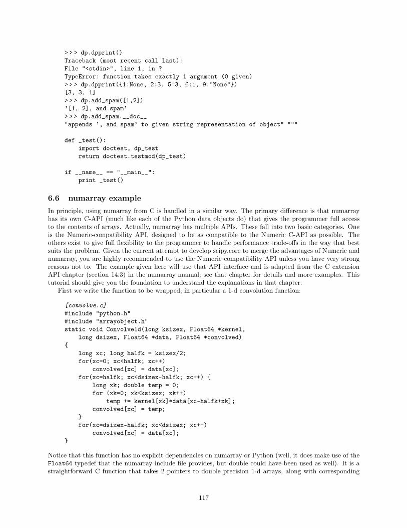
> > > dp.dpprint()Traceback (most recent call last):File "<stdin>", line 1, in ?TypeError: function takes exactly 1 argument (0 given)> > > dp.dpprint({1:None, 2:3, 5:3, 6:1, 9:"None"})[3, 3, 1]> > > dp.add_spam([1,2])’[1, 2], and spam’> > > dp.add_spam.__doc__"appends ’, and spam’ to given string representation of object" """

def _test():import doctest, dp_testreturn doctest.testmod(dp_test)

if __name__ == "__main__":print _test()

6.6 numarray exampleIn principle, using numarray from C is handled in a similar way. The primary difference is that numarrayhas its own C-API (much like each of the Python data objects do) that gives the programmer full accessto the contents of arrays. Actually, numarray has multiple APIs. These fall into two basic categories. Oneis the Numeric-compatibility API, designed to be as compatible to the Numeric C-API as possible. Theothers exist to give full flexibility to the programmer to handle performance trade-offs in the way that bestsuits the problem. Given the current attempt to develop scipy.core to merge the advantages of Numeric andnumarray, you are highly recommended to use the Numeric compatibility API unless you have very strongreasons not to. The example given here will use that API interface and is adapted from the C extensionAPI chapter (section 14.3) in the numarray manual; see that chapter for details and more examples. Thistutorial should give you the foundation to understand the explanations in that chapter.

First we write the function to be wrapped; in particular a 1-d convolution function:

[convolve.c]#include "python.h"#include "arrayobject.h"static void Convolve1d(long ksizex, Float64 *kernel,

long dsizex, Float64 *data, Float64 *convolved){

long xc; long halfk = ksizex/2;for(xc=0; xc<halfk; xc++)

convolved[xc] = data[xc];for(xc=halfk; xc<dsizex-halfk; xc++) {

long xk; double temp = 0;for (xk=0; xk<ksizex; xk++)

temp += kernel[xk]*data[xc-halfk+xk];convolved[xc] = temp;

}for(xc=dsizex-halfk; xc<dsizex; xc++)

convolved[xc] = data[xc];}

Notice that this function has no explicit dependencies on numarray or Python (well, it does make use of theFloat64 typedef that the numarray include file provides, but double could have been used as well). It is astraightforward C function that takes 2 pointers to double precision 1-d arrays, along with corresponding

117

sizes for the arrays, and a pointer to the output array of the same type and size as the input array (notkernel).

The following begins the wrapper part of the file.

static PyObject *Py_Convolve1d(PyObject *obj, PyObject *args){

PyObject *okernel, *odata;PyArrayObject *kernel, *data, *convolved;if (!PyArg_ParseTuple(args, "OO", &okernel, &odata)) {

return PyErr_Format(_Error,"Convolve1d: Invalid parameters."); goto _fail;

}

Two PyObject pointers are defined for the two expected arguments, and the object pointers for thosearguments are obtained.

kernel = (PyArrayObject *) PyArray_ContiguousFromObject(okernel, tFloat64, 1, 1);

data = (PyArrayObject *) PyArray_ContiguousFromObject(odata, tFloat64, 1, 1);

if (!kernel || !data) goto _fail;

What happens in this part of the code needs some background explanation. Typically a C programmerexpects arrays to be a simple, contiguous array of values in memory, and in the C context, this is the normalconvention. But what numarray considers arrays may not be this simple. Arrays may not be contiguous sincea sliced, strided view of an array defines an array to be to be non-contiguous series of values. What’s more,the values in the array may be byte-swapped from the native representation of the processor, and it maynot even be properly memory-aligned. Dealing with such arrays places a large burden on the programmerto iterate through all the values in the array (something numarray handles behind the scenes).

The two calls to PyArray_ContiguousFromObject for each of the respective arguments first ensures thatthe argument is an array or a Python object that can be cast into an array (e.g., a Python list). If not,a NULL value is returned. If the argument is an array which is not contiguous, properly byte-ordered, oraligned, then a copy of the array will be generated that is. If the type specified in the function call is differentthan the type of the array (the presence of tFloat64 indicates that a Float64 array is being requested), acopy will also be made. The 3rd and 4th arguments specify the minimum and maximum acceptable valuesfor the number of dimensions. If the input array is the right type and satisfies the other conditions, thefunction simply returns the input argument, otherwise it returns the pointer to the new array copy. In short,these function calls ensure you get data in an easily used form and of the type requested.

convolved = (PyArrayObject *) PyArray_FromDims(data->nd, data->dimensions, tFloat64);

if (!convolved) goto _fail;

The PyArray_FromDims function call creates a new array from scratch given the specified shape and type.At this point it is worth pointing out that the ’array’ pointers are not themselves pointers to C arrays butinstead pointers to Python data structures. This data structure contains information about the array suchas where the actual array data are located, the type, number of dimensions, the size of each dimension,strides, and other information. This information is outlined in the previously referenced numarray section(14.2.4). We will only refer to those structure members necessary for this simple example. So the member ndrefers to the number of dimensions and the member dimensions is a pointer to an array of data dimensions(of length nd). After this preparation, we are ready to call the function that we wrote to actually do thecomputation, now using the data member of the array structure that points to the data array.

Convolve1d(kernel->dimensions[0], kernel->data,data->dimensions[0], data->data, convolved->data);

118

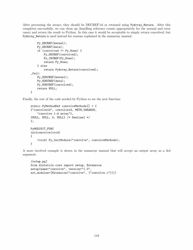
After processing the arrays, they should be DECREF’ed or returned using PyArray_Return. After thiscompletes successfully, we can clean up (handling reference counts appropriately for the normal and errorcases) and return the result to Python. In this case it would be acceptable to simply return convolved, butPyArray_Return is used instead for reasons explained in the numarray manual.

Py_DECREF(kernel);Py_DECREF(data);if (convolved != Py_None) {

Py_DECREF(convolved);Py_INCREF(Py_None);return Py_None;

} elsereturn PyArray_Return(convolved);

_fail:Py_XDECREF(kernel);Py_XDECREF(data);Py_XDECREF(convolved);return NULL;

}

Finally, the rest of the code needed by Python to see the new function:

static PyMethodDef convolveMethods[] = {{"convolve1d", convolve1d, METH_VARARGS,

"convolve 1-d array"},{NULL, NULL, 0, NULL} /* Sentinel */};

PyMODINIT_FUNCinitconvolve(void){

(void) Py_InitModule("convolve", convolveMethods);}

A more involved example is shown in the numarray manual that will accept an output array as a 3rdargument.

[setup.py]from distutils.core import setup, Extensionsetup(name="convolve", version="1.0",ext_modules=[Extension("convolve", ["convolve.c"])])

119

AcknowledgementsThanks to Phil Hodge, JC Hsu, Vicki Laidler, Todd Miller, Warren Hack, Dave Grumm, and Ivo Busko forvaluable comments on previous versions of this document.

120

Appendix A: Python Books, Tutorials, and On-line ResourcesThe Python web site (www.python.org) contains pointers to a great deal of information about Pythonincluding its standard documentation, conferences, books, tutorials, etc. In particular, the following linkswill contain up-to-date lists of books and tutorials:

• Books: www.python.org/moin/PythonBooks

• Tutorials: www.python.org/doc/Intros.html (all online)

Books of note for beginners that have some programming experience:

• Learning Python (2nd ed) Lutz & Ascher: Probably the standard introductory book

• The Quick Python Book by Harms & McDonald: some prefer the style of this one

• Python: Visual QuickStart Guide by Fehily: and others this one

• Dive Into Python: Python for Experienced Programmers by Pilgrim (free on-line version also available)

On-line tutorials or books:

• An Introduction to Python by van Rossum: The original tutorial

• A Byte of Python by Swaroop: essentially an on-line book.

• A Quick Tour of Python by Greenfield and White:http://stsdas.stsci.edu/pyraf/doc/python_quick_tour (A bit dated but comparatively brief). PDFalso available.

Reference books:

• Python Essential Reference (2nd ed.) by Beazley

• Python in a Nutshell by Martelli

• Python Library Documentation (available free on-line)

Mailing lists:

• astropy: For astronomical packages (e.g. PyRAF, PyFITS, numdisplay):http://www.scipy.net/mailman/listinfo/astropy

• numarray: http://sourceforge.net/mail/?group_id=1369

• matplotlib: http://sourceforge.net/mail/?group_id=80706

• ipython: http://www.scipy.net/pipermail/ipython-user/

Manuals for numarray, PyFITS, PyRAF, ipython, and matplotlib are all available. Google PyFITS, nu-marray or PYRAF with “manual” to find those. The matplotlib User Guide is available on a link from thehome page (Google “matplotlib”). The ipython manual is available from ipython.scipy.org. The numdisplayinstructions are available at: http://stsdas.stsci.edu/numdisplay/doc/numdisplay_help.html

121

Appendix B: Why would I switch from IDL to Python (or not)?We do not claim that all, or even most, current IDL users should switch to using Python now. IDL suitsmany people’s needs very well and we recognize that there must be a strong motivation for starting to usePython over IDL. This appendix will present the pros and cons of each so that users can make a betterinformed decision about whether they should consider using Python. At the end we give a few cases wherewe feel users should give serious consideration to using Python over IDL.

Pros and Cons of eachThese are addressed in a comparative sense. Attributes that both share, e.g.., that they are interpreted andrelatively slow for very simple operations, are not listed.

Pros of IDL:

• Mature many numerical and astronomical libraries available

• Wide astronomical user base

• Numerical aspect well integrated with language itself

• Many local users with deep experience

• Faster for small arrays

• Easier installation

• Good, unified documentation

• Standard GUI run/debug tool (IDLDE)

• Single widget system (no angst about which to choose or learn)

• SAVE/RESTORE capability

• Use of keyword arguments as flags more convenient

Cons of IDL:

• Narrow applicability, not well suited to general programming

• Slower for large arrays

• Array functionality less powerful

• Table support poor

• Limited ability to extend using C or Fortran, such extensions hard to distribute and support

• Expensive, sometimes problem collaborating with others that don’t have or can’t afford licences.

• Closed source (only RSI can fix bugs)

• Very awkward to integrate with IRAF tasks

• Memory management more awkward

• Single widget system (useless if working within another framework)

• Plotting:

– Awkward support for symbols and math text– Many font systems, portability issues (v5.1 alleviates somewhat)– not as flexible or as extensible– plot windows not intrinsically interactive (e.g., pan & zoom)

122

Pros of Python:

• Very general and powerful programming language, yet easy to learn. Strong, but optional, ObjectOriented programming support

• Very large user and developer community, very extensive and broad library base

• Very extensible with C, C++, or Fortran, portable distribution mechanisms available

• Free; non-restrictive license; Open Source

• Becoming the standard scripting language for astronomy

• Easy to use with IRAF tasks

• Basis of STScI application efforts

• More general array capabilities

• Faster for large arrays, better support for memory mapping

• Many books and on-line documentation resources available (for the language and its libraries)

• Better support for table structures

• Plotting

– framework (matplotlib) more extensible and general

– Better font support and portability (only one way to do it too)

– Usable within many windowing frameworks (GTK, Tk, WX, Qt...)

– Standard plotting functionality independent of framework used

– plots are embeddable within other GUIs

– more powerful image handling (multiple simultaneous LUTS, optional resampling/rescaling, alphablending, etc)

• Support for many widget systems

• Strong local influence over capabilities being developed for Python

Cons of Python:

• More items to install separately

• Not as well accepted in astronomical community (but support clearly growing)

• Scientific libraries not as mature:

– Documentation not as complete, not as unified

– Numeric/numarray split

– Not as deep in astronomical libraries and utilities

– Not all IDL numerical library functions have corresponding functionality in Python

• Some numeric constructs not quite as consistent with language (or slightly less convenient than IDL)

• Array indexing convention “backwards”

• Small array performance slower

• No standard GUI run/debug tool

123

• Support for many widget systems (angst regarding which to choose)

• Current lack of function equivalent to SAVE/RESTORE in IDL

• matplotlib does not yet have equivalents for all IDL 2-D plotting capability (e.g., surface plots)

• Use of keyword arguments used as flags less convenient

• Plotting:

– comparatively immature, still much development going on

– missing some plot type (e.g., surface)

– 3-d capability requires VTK

Specific cases

Here are some specific instances where using Python provides strong advantages over IDL

• Your processing needs depend on running a few hard-to-replicate IRAF tasks, but you don’t want todo most of your data manipulation in IRAF, but would rather write your own IDL-style programs todo so (and soon other systems will be accessible from Python, e.g., MIDAS, ALMA, slang, etc)

• You have algorithms that cannot be efficiently coded in IDL. They likely won’t be efficiently coded inPython either, but you will find interfacing the needed C or Fortran code easier, more flexible, moreportable, and distributable. (Question: how many distributed IDL libraries developed by 3rd partiesinclude C or Fortran code?) Or you need to wrap existing C libraries (Python has many tools to makethis easier to do).

• You do work on algorithms that may migrate into STSDAS packages. Using Python means that yourwork will be more easily adapted as a distributed and supported tool.

• You wish to integrate data processing with other significant non-numerical processing such as databases,web page generation, web services, text processing, process control, etc.

• You want to learn object-oriented programming and use it with your data analysis. (But you don’tneed to learn object-oriented programming to do data analysis in Python.)

• You want to be able to use the same language you use for data analysis for most of your other scriptingand programming tasks.

• Your boss makes you.

• You want to be a cool, with-it person.

• You are honked off at ITT Space Systems/RSI.

Obviously using a new language and libraries entails time spent learning. Despite what people say, it’s neverthat easy, especially if one has a lot of experience and code invested in an existing language. If you don’thave any strong motivations to switch, you should probably wait.

124

Appendix C: IDL/numarray feature mapping

IDL Python Equivalent.run import (.py assumed)

reload(module) # to recompile/re-executeipython: run

@<filename> execfile(’fileame’)ipython: run

exit control-D (MS windows: control-Z)ipython: Quit or Exit

up-arrow (command recall) up-arrow

Operators<,> (clipping)a < 100.a > 100.

Currently no operator equivalent. The functionalequivalent is choose(a<100, (a, 100.))

MOD %# (matrix multiply) multiply.outer() is equivalent for some applications,

matrixmultiply() for others.^ **

Boolean operatorsand no operator equivalent

Python and operator is not the same!or no operator equivalent

Python or operator is not the same!not no operator equivalent

Python not operator is not the same!

Comparison operators.EQ. ==.NE. !=.LT. <.LE. <=.GT. >.GE. >=

Bitwise operatorsand &or |xor ^not ~ishift(a,1) a< <1ishift(a,-1) a> >1

Slicing and indexing Note: order of indices is opposite!a(i,j) (IDL) equivalent to a[j,i] (Python)

i:j i:j (j element not part of slice)i:* i:*:i :ia(i,*) a[:,i]a(i:j:s) a[i:j:s]

125

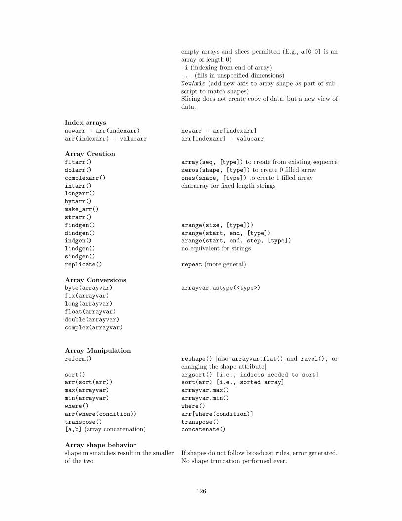
empty arrays and slices permitted (E.g., a[0:0] is anarray of length 0)-i (indexing from end of array)... (fills in unspecified dimensions)NewAxis (add new axis to array shape as part of sub-script to match shapes)Slicing does not create copy of data, but a new view ofdata.

Index arraysnewarr = arr(indexarr) newarr = arr[indexarr]arr(indexarr) = valuearr arr[indexarr] = valuearr

Array Creationfltarr()dblarr()complexarr()intarr()longarr()bytarr()make_arr()strarr()

array(seq, [type]) to create from existing sequencezeros(shape, [type]) to create 0 filled arrayones(shape, [type]) to create 1 filled arraychararray for fixed length strings

findgen()dindgen()indgen()lindgen()sindgen()

arange(size, [type]))arange(start, end, [type])arange(start, end, step, [type])no equivalent for strings

replicate() repeat (more general)

Array Conversionsbyte(arrayvar)fix(arrayvar)long(arrayvar)float(arrayvar)double(arrayvar)complex(arrayvar)

arrayvar.astype(<type>)

Array Manipulationreform() reshape() [also arrayvar.flat() and ravel(), or

changing the shape attribute]sort() argsort() [i.e., indices needed to sort]arr(sort(arr)) sort(arr) [i.e., sorted array]max(arrayvar) arrayvar.max()min(arrayvar) arrayvar.min()where() where()arr(where(condition)) arr[where(condition)]transpose() transpose()[a,b] (array concatenation) concatenate()

Array shape behaviorshape mismatches result in the smallerof the two

If shapes do not follow broadcast rules, error generated.No shape truncation performed ever.

126

Numeric typesbyte Int8

UInt8 (unsigned)int Int16long Int32float Float32double Float64complex Complex64

Complex128UInt16UInt32Int64UInt64

Math Functionsabs() abs()acos() arccos()alog() log()alog10() log10()asin() arcsin()atan() arctan()atan(y,x) arctan2()ceil() ceil()conj() conjugate()cos() cos()cosh() cosh()exp() exp()floor() floor()imaginary() complexarr.imag (.real for real component)invert() Matrix moduleishift() right_shift(), left_shift()round() round()sin() sin()sinh() sinh()sqrt() sqrt()tan() tan()tanh() tanh()

fft() fft (fft module)convol() convolve() (convolve module)randomu() random(), uniform() (random_array module)randomn() normal() (random_array module)

Programmingexecute() exec()n_elements(arrayvar) arrayvar.nelements()n_params() closest equivalent is len(*args). Ability to supply

default values for parameters replaces some uses ofn_params()

size() .shape attribute, .type() methodwait time.sleep (time module)

127

Appendix D: matplotlib for IDL UsersAuthor: Vicki Laidler

This is not a complete discussion of the power of matplotlib (the OO machinery) or pylab (the functionalinterface). This document only provides a translation from common IDL plotting functionality, and mentionsa few of the additional capabilities provided by pylab. For a more complete discussion, you will eventuallywant to see the tutorial and the documentation for the pylab interface:

http://matplotlib.sourceforge.net/tutorial.htmlhttp://matplotlib.sourceforge.net/matplotlib.pylab.html

Setting up and customizing your Python environment:Whether you use PyRAF, IPython, or the default python interpreter, there are ways to automatically importyour favorite modules at startup using a configuration file. See the documentation for those packages fordetails. The examples in this document will explicitly import all packages used.

Setting up and customizing matplotlib:You will want to modify your .matplotlibrc plot to use the correct backend for plotting, and to setsome default behaviors. (The STScI versions of the default .matplotlibrc have already been modified toincorporate many of these changes.) If there is a .matplotlibrc file in your current directory, it will be usedinstead of the file in your home directory. This permits setting up different default environments for differentpurposes. You may also want to change the default behavior for image display to avoid interpolating, andset the image so that pixel (0,0) appears in the lower left of the window.

image.interpolation : nearest # see help(imshow) for optionsimage.origin : lower # lower | upper

I also wanted to change the default colors and symbols.

lines.marker : None # like !psym=0; plots are line plotsby default

lines.color : k # blacklines.markerfacecolor : k # blacklines.markeredgecolor : k # blacktext.color : k # black

Symbols will be solid colored, not hollow, unless you change markerfacecolor to match the color of thebackground.

About overplotting behavior:

The default behavior for matplotlib is that every plot is a "smart” overplot, stretching the axes if necessary;and one must explicitly clear the axes, or clear the figure, to start a new plot. It’s possible to change thisbehavior in the setup file, to get new plots by default

axes.hold : False # whether to clear the axes bydefault on

and override it by specifying the "hold" keyword in the plotting call. However I DO NOT recommend this;it takes a bit of getting used to, but I found it easier to completely change paradigms to "build up the plotpiece by piece" than it is to remember which commands will decorate an existing plot and which won’t.

128

Some philosophical differences:

Matplotlib tends towards atomic commands to control each plot element independently, rather than keywordson a plot command. This takes getting used to, but adds versatility. Thus, it may take more commandsto accomplish something in matplotlib than it does in IDL, but the advantage is that these commands canbe done in any order, or repeatedly tweaked until it’s just right. This is particularly apparent when makinghardcopy plots: the mode of operation is to tweak the plot until it looks the way you want, then press abutton to save it to disk. Since the pylab interface is essentially a set of convenience functions layered on topof the OO machinery, sometimes by different developers, there is occasionally a little bit of inconsistency inhow things work between different functions. For instance the errorbar function violates the principle inthe previous paragraph: it’s not an atomic function that can be added to an existing plot; and the scatterfunction is more restrictive in its argument set than the plot function, but offers a couple of different keywordsthat add power.

Some syntactic differences:

You can NOT abbreviate a keyword argument in matplotlib. Some keywords have had some shorthandversions programmed in as alternates - for instance lw=2 instead of linewidth=2 - but you need to knowthe shorthand. Python uses indentation for loop control; leading spaces will cause an error if you are at theinteractive command line. To issue 2 commands on the same line, use a semicolon instead of an ampersand.

The Rosetta Stone:

IDL MatplotlibSetup (none needed if your paths

are correct)from numarray import *from pylab import *import pyfits(Or, none needed if you setup your favorite modules inthe configuration file forthe Python environment you’reusing.)

Some data sets: foo = indgen(20)bar = foo*2

foo = arange(20)bar = foo*2

Basic plotting: plot, foo plot(foo)plot, foo, bar plot(foo, bar)plot, foo, bar,line=1, thick=2

plot(foo, bar, ’–’, lw=2)***or spell out linewidth=2

plot, foo, bar, ticklen=1 plot(foo, bar)grid()

plot, foo, bar, psym=1 plot(foo, bar, ’x’)ORscatter(foo, bar)

plot, foo, bar, psym=-1,symsize=3

plot(foo, bar, ’-x’, ms=5)***or spell out markersize=5

plot, foo, bar,xran=[2,10], yran=[2,10]

plot(foo, bar)xlim(2,10)ylim(2,10)

err=indgen(20)/10. err = arange(20)/10.

129

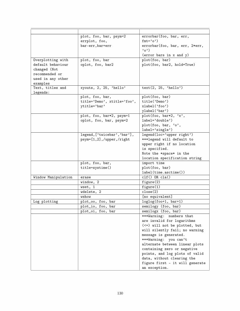
plot, foo, bar, psym=2errplot, foo,bar-err,bar+err

errorbar(foo, bar, err,fmt=’o’)errorbar(foo, bar, err, 2*err,’o’)(error bars in x and y)

Overplotting withdefault behaviourchanged (Notrecommended orused in any otherexamples

plot, foo, baroplot, foo, bar2

plot(foo, bar)plot(foo, bar2, hold=True)

Text, titles andlegends:

xyouts, 2, 25, ’hello’ text(2, 25, ’hello’)

plot, foo, bar,title=’Demo’, xtitle=’foo’,ytitle=’bar’

plot(foo, bar)title(’Demo’)xlabel(’foo’)ylabel(’bar’)

plot, foo, bar*2, psym=1oplot, foo, bar, psym=2

plot(foo, bar*2, ’x’,label=’double’)plot(foo, bar, ’o’,label=’single’)

legend,[’twicebar’,’bar’],psym=[1,2],/upper,/right

legend(loc=’upper right’)***legend will default toupper right if no locationis specified.Note the *space* in thelocation specification string

plot, foo, bar,title=systime()

import timeplot(foo, bar)label(time.asctime())

Window Manipulation erase clf() OR cla()window, 2 figure(2)wset, 1 figure(1)wdelete, 2 close(2)wshow [no equivalent]

Log plotting plot_oo, foo, bar loglog(foo+1, bar+1)plot_io, foo, bar semilogy (foo, bar)plot_oi, foo, bar semilogx (foo, bar)

***Warning: numbers thatare invalid for logarithms(<=) will not be plotted, butwill silently fail; no warningmessage is generated.***Warning: you can’talternate between linear plotscontaining zero or negativepoints, and log plots of validdata, without clearing thefigure first - it will generatean exception.

130

Postscript output set_plot, ’ps’device,file=’myplot.ps’,/landplot, foo, bardevice,/close

plot(foo, bar)savefig(’myplot.ps’,orientation=’landscape’)

Viewing imagedata:

im = mrdfits(’myfile.fits’,1)

tv, imloadct, 5loadct, 0contour, imxloadct

f = pyfits.open(’myfile.fits’)im = f[1].dataimshow(im)jet()gray()contour(im)[no equivalent]

Histograms mu=100 & sigma=15 &x=fltarr(10000)seed=123132for i = 0, 9999 do x[i] =mu + sigma*randomn(seed)plothist, x

mu, sigma = 10, 15x = mu + sigma*randn(10000)n, bins, patches = hist(x, 50)

*** Note that histograms are specified a bitdifferently and also look a bit different: bar chartinstead of skyline style

Multiple plots on apage

!p.multi=[4,2,2]plot, foo, barplot, bar, fooplot, foo, 20*fooplot, foo, bar*foo

subplot(221) ; plot(foo, bar)subplot(222) ; plot(bar, foo)subplot(223) ; plot(foo,20*foo)subplot(224) ; plot(foo,bar*foo)

Erasing andredrawing asubplot:

[no equivalent] subplot(222)cla()scatter(bar, foo)

plotting x, y, colorand size:

[no obvious equivalent] scatter(foo, bar, c=foo+bar,s=10*foo)

Adding a colorbar [no obvious equivalent] colorbar()

Some comparisons:Some additional functionality:

• modify axes without replotting

• add labels, generate hardcopy, without replotting

• colored lines and points, many more point styles

• smarter legends

• TEX-style math symbols supported

• interactive pan/zoom

131

Some functionality that is not yet conveniently wrapped:

(These are items that are available through the OO machinery, but are not yet wrapped into convenientfunctions for the interactive user. We welcome feedback on which of these would be most important oruseful!)

• subtitles

• loadct - to dynamically modify or flick through colortables

• tvrdc,x,y - to read the xy position of the cursor (will soon be available)

• histogram specification by bin interval rather than number of bins

Some still-missing functionality:

(These are items for which the machinery has not yet been developed.)

• surface plots

• save - to save everything in an environment (will soon be available)

• journal - to capture commands & responses. (ipython can capture commands.)

Symbols, line styles, and colors:

!psym equivalences:

0 line -

1 plus +

2 asterisk unsupported; overplotting + with x is close

3 dot .

4 diamond d

5 triangle ^

6 square s

7 cross x

10 histogram ls=’steps’

!linestyle equivalences:

1 solid -

2 dotted :

3 dashed --

4 dash-dot -.

The following line styles are supported:

- : solid line

-- : dashed line

-. : dash-dot line

132

: : dotted line

. : points

, : pixels

o : circle symbols

^ : triangle up symbols

v : triangle down symbols

< : triangle left symbols

> : triangle right symbols

s : square symbols

+ : plus symbols

x : cross symbols

D : diamond symbols

d : thin diamond symbols

1 : tripod down symbols

2 : tripod up symbols

3 : tripod left symbols

4 : tripod right symbols

h : hexagon symbols

H : rotated hexagon symbols

p : pentagon symbols

| : vertical line symbols

_ : horizontal line symbols

steps : use gnuplot style ’steps’ # kwarg only

The following color strings are supported

b : blue

g : green

r : red

c : cyan

m : magenta

y : yellow

k : black

w : white

Matplotlib also accepts rgb and colorname specifications (eg hex rgb, or "white").

133

Approximate color table equivalences:

loadct,0 gray()

loadct,1 almost bone()

loadct,3 almost copper()

loadct,13 almost jet()

Color tables for images:

autumn

bone

cool

copper

flag

gray

hot

hsv

jet

pink

prism

spring

summer

winter

134

Appendix E: Editors and Integrated Development Environments

EditorsPython is easier to use with a good editor. Since indentation is important in Python, use of an editor thatsupports block indentation (indenting and undoing indentation for a block of lines) is very handy. Alsoimportant is using an editor that can automatically convert tabs to spaces (the recommended means ofindenting). Fortunately, a great variety of editors handle both these requirements. Many editors providemany more features that make Python easier to code including syntax highlighting, code folding, auto-completion, etc. See http://wiki.python.org/moin/PythonEditors for a list of editors that have good supportfor Python.

Integrated Development EnvironmentsThe use of IDEs with Python is not as widespread as it is for other languages (particularly Java). Somewould explain that by saying that Python doesn’t require IDE’s as much (or doesn’t benefit as much) asother languages. It may be the culture, and certainly it is at least partly due to the fact that the user baseis smaller than more widely used languages (thus fewer resources available to devote to IDEs on either theopen source or commercial front). Nevertheless, there are IDE’s available for Python, both open source andcommercial. Generally speaking, IDEs provide class browsing features, a debugger, code completion as wellas more advanced editing features. It is questionable whether these sorts of features are worth the effortexpended on learning how to use them if your use of Python is not heavy, especially if you are not developingcomplex projects.

IDLE is one that is distributed with Python. Pythonwin is one that is also open source, but only runsunder Microsoft windows. In many respects emacs serves as an IDE if you willing to learn how to use it.BoaConstrictor and Eric3 are the other best known. Wing IDE, BlackAdder, and Komodo are the most wellknown commercial IDE’s for Python; these generally have many more features than the opensource IDEs.Wing IDE is significantly cheaper for educational institutions (~$100 per developer per platform). All threeare very inexpensive for students and individual (non-work, non-commercial) use (~$30). Google any ofthese names (with Python also in the search box) to get more information.

135

Appendix F: Numeric vs numarray vs scipy vs Numeric3...In the beginning there was Numeric, which was the first array package available for Python. Because ofvarious shortcomings that made it more awkward to use for larger arrays, STScI developed numarray. Sinceeach has advantages over the other, there has not been any clear indication that all Numeric users are willingto move to numarray (primarily because numarray is slower for small arrays than Numeric). This situationhas led to a schism in library support where many useful libraries are available for one or the other.

Currently there is an effort on STScI’s part to make it easy for these libraries to support both Numericand numarray (simultaneously). Matplotlib already supports both, and we are currently working to makethe largest library suite, scipy, compatible with numarray (parts are already usable with numarray, but notreleased yet). We see the interoperability issue improving greatly over the next year. Some modules, by theirnature, won’t ever work with Numeric, such as PyFITS since they depend on features that only numarrayhas.

Concurrently, there is an effort to merge the advantages of both array packages into one system, whichis currently being referred to by two different names: Numeric3 or scipy.core. It isn’t entirely clear howlong this will take (it is hoped to be completed this year). This new version will encompass all the existingfeatures of numarray; generally speaking, it’s user interface and feature set will be very similar to numarray(rather than that for Numeric). When this project is completed, this should end the existing split betweenthe two packages.

136