Machine Learning with Python Tutorial
453
bodenseo Machine Learning with Python Tutorial by Bernd Klein
-
Upload
khangminh22 -
Category
Documents
-
view
1 -
download
0
Transcript of Machine Learning with Python Tutorial

bodenseo
Machine Learning withPython Tutorial
byBernd Klein

© 2021 Bernd Klein
All rights reserved. No portion of this book may be reproduced or used in any manner without written permission from the copyright owner.
For more information, contact address: [email protected]
www.python-course.eu

Python CourseMachine Learning
With Python byBernd Klein
Machine Learning Terminology .................................................................................................3Representation and Visualization of Data ................................................................................15Loading the Iris Data with Scikit-learn ....................................................................................18Visualising the Features of the Iris Data Set.............................................................................23Scatterplot 'Matrices .................................................................................................................27Datasets in sklearn ....................................................................................................................29Loading Digits Data..................................................................................................................31Reading the data and conversion back into 'data' and 'labels'...................................................51Other Interesting Distributions .................................................................................................54k-Nearest-Neighbor Classifier ..................................................................................................72From Dividing Lines to Neural Networks................................................................................96Neural Networks, Structure, Weights and Matrices ...............................................................141Running a Neural Network with Python ................................................................................153Backpropagation in Neural Networks ....................................................................................162Training a Neural Network with Python ................................................................................169Softmax as Activation Function .............................................................................................182Confusion Matrix........................................................................................................................3Neural Network ......................................................................................................................198Multiple Runs .........................................................................................................................210With Bias Nodes .....................................................................................................................216Networks with multiple hidden layers....................................................................................227Networks with multiple hidden layers and Epochs ................................................................231A Neural Network for the Digits Dataset ...............................................................................269Naive Bayes Classifier with Scikit .........................................................................................316Regression Trees.....................................................................................................................413The maths behind regression trees..........................................................................................418Regression Decision Trees from scratch in Python................................................................423Regression Trees in sklearn ....................................................................................................434TensorFlow .............................................................................................................................437

2

M A C H I N E L E A R N I N G T E R M I N O L O G Y
CLASSIFIER
A program or a function which maps from unlabeled instances to classes is called a classifier.
CONFUSION MATRIX
A confusion matrix, also called a contingeny table or error matrix, is used to visualize the performance of aclassifier.
The columns of the matrix represent the instances of the predicted classes and the rows represent the instancesof the actual class. (Note: It can be the other way around as well.)
In the case of binary classification the table has 2 rows and 2 columns.
Example:
3

ConfusionMatrix
Predicted classes
male female
Actu
alclasses
male 42 8
female 18 32
This means that the classifier correctly predicted a male person in 42 cases and it wrongly predicted 8 maleinstances as female. It correctly predicted 32 instances as female. 18 cases had been wrongly predicted as maleinstead of female.
ACCURACY (ERROR RATE)
Accuracy is a statistical measure which is defined as the quotient of correct predictions made by a classifierdivided by the sum of predictions made by the classifier.
The classifier in our previous example predicted correctly predicted 42 male instances and 32 female instance.
Therefore, the accuracy can be calculated by:
accuracy = (42 + 32) / (42 + 8 + 18 + 32)
which is 0.72
Let's assume we have a classifier, which always predicts "female". We have an accuracy of 50 % in this case.
ConfusionMatrix
Predicted classes
male femaleA
ctual
classes
male 0 50
female 0 50
We will demonstrate the so-called accuracy paradox.
A spam recogition classifier is described by the following confusion matrix:
4

ConfusionMatrix
Predicted classes
spam ham
Actu
alclasses
spam 4 1
ham 4 91
The accuracy of this classifier is (4 + 91) / 100, i.e. 95 %.
The following classifier predicts solely "ham" and has the same accuracy.
ConfusionMatrix
Predicted classes
spam ham
Actu
alclasses
spam 0 5
ham 0 95
The accuracy of this classifier is 95%, even though it is not capable of recognizing any spam at all.
PRECISION AND RECALL
ConfusionMatrix
Predicted classes
negative positive
Actu
alclasses
negative TN FP
positive FN TP
Accuracy: (TN + TP) / (TN + TP + FN + FP)
Precision: TP / (TP + FP)
5

Recall: TP / (TP + FN)
SUPERVISED LEARNING
The machine learning program is both given the input data and the corresponding labelling. This means thatthe learn data has to be labelled by a human being beforehand.
UNSUPERVISED LEARNING
No labels are provided to the learning algorithm. The algorithm has to figure out the a clustering of the inputdata.
REINFORCEMENT LEARNING
A computer program dynamically interacts with its environment. This means that the program receivespositive and/or negative feedback to improve it performance.
6

E V A L U A T I O N M E T R I C S
INTRODUCTION
Not only in machine learning but also ingeneral life, especially business life, youwill hear questiones like "How accurate isyour product?" or "How precise is yourmachine?". When people get replies like"This is the most accurate product in itsfield!" or "This machine has the highestimaginable precision!", they feelfomforted by both answers. Shouldn'tthey? Indeed, the terms accurate andprecise are very often used
interchangeably. We will give exactdefinitions later in the text, but in anutshell, we can say: Accuracy is ameasure for the closeness of somemeasurements to a specific value, whileprecision is the closeness of the measurements to each other.
These terms are also of extreme importance in Machine Learning. We need them for evaluating MLalgorithms or better their results.
We will present in this chapter of our Python Machine Learning Tutorial four important metrics. These metricsare used to evaluate the results of classifications. The metrics are:
• Accuracy• Precision• Recall• F1-Score
We will introduce each of these metrics and we will discuss the pro and cons of each of them. Each metricmeasures something different about a classifiers performance. The metrics will be of outmost importance forall the chapters of our machine learning tutorial.
ACCURACY
Accuracy is a measure for the closeness of the measurements to a specific value, while precision is thecloseness of the measurements to each other, i.e. not necessarily to a specific value. To put it in other words: Ifwe have a set of data points from repeated measurements of the same quantity, the set is said to be accurate iftheir average is close to the true value of the quantity being measured. On the other hand, we call the set to beprecise, if the values are close to each other. The two concepts are independent of each other, which meansthat the set of data can be accurate, or precise, or both, or neither. We show this in the following diagram:
7

CONFUSION MATRIX
Before we continue with the term accuracy , we want to make sure that you understand what a confusionmatrix is about.
A confusion matrix, also called a contingeny table or error matrix, is used to visualize the performance of aclassifier.
The columns of the matrix represent the instances of the predicted classes and the rows represent the instancesof the actual class. (Note: It can be the other way around as well.)
In the case of binary classification the table has 2 rows and 2 columns.
8

We want to demonstrate the concept with an example.
Example:
ConfusionMatrix
Predicted classes
cat dog
Actu
alclasses
cat 42 8
dog 18 32
This means that the classifier correctly predicted a cat in 42 cases and it wrongly predicted 8 cat instances asdog. It correctly predicted 32 instances as dog. 18 cases had been wrongly predicted as cat instead of dog.
ACCURACY IN CLASSIFICATION
We are interested in Machine Learning and accuracy is also used as a statistical measure. Accuracy is astatistical measure which is defined as the quotient of correct predictions (both True positives (TP) and Truenegatives (TN)) made by a classifier divided by the sum of all predictions made by the classifier, includingFalse positves (FP) and False negatives (FN). Therefore, the formula for quantifying binary accuracy is:
accuracy =TP + TN
TP + TN + FP + FN
where: TP = True positive; FP = False positive; TN = True negative; FN = False negative
The corresponding Confusion Matrix looks like this:
ConfusionMatrix
Predicted classes
negative positive
Actu
alclasses
negative TN FP
positive FN TP
We will now calculate the accuracy for the cat-and-dog classification results. Instead of "True" and "False",we see here "cat" and "dog". We can calculate the accuracy like this:
9

TP = 42TN = 32FP = 8FN = 18
Accuracy = (TP + TN)/(TP + TN + FP + FN)print(Accuracy)
Let's assume we have a classifier, which always predicts "dog".
ConfusionMatrix
Predicted classes
cat dog
Actu
alclasses
cat 0 50
dog 0 50
We have an accuracy of 0.5 in this case:
TP, TN, FP, FN = 0, 50, 50, 0Accuracy = (TP + TN)/(TP + TN + FP + FN)print(Accuracy)
ACCURACY PARADOX
We will demonstrate the so-called accuracy paradox.
A spam recogition classifier is described by the following confusion matrix:
ConfusionMatrix
Predicted classes
spam ham
Actu
alclasses
spam 4 1
ham 4 91
0.74
0.5
10

TP, TN, FP, FN = 4, 91, 1, 4accuracy = (TP + TN)/(TP + TN + FP + FN)print(accuracy)
The following classifier predicts solely "ham" and has the same accuracy.
ConfusionMatrix
Predicted classes
spam ham
Actu
alclasses
spam 0 5
ham 0 95
TP, TN, FP, FN = 0, 95, 5, 0accuracy = (TP + TN)/(TP + TN + FP + FN)print(accuracy)
The accuracy of this classifier is 95%, even though it is not capable of recognizing any spam at all.
PRECISION
Precision is the ratio of the correctly identified positive cases to all the predicted positive cases, i.e. thecorrectly and the incorrectly cases predicted as positive . Precision is the fraction of retrieved documentsthat are relevant to the query. The formula:
precision =TP
TP + FP
We will demonstrate this with an example.
ConfusionMatrix
Predicted classes
spam ham
Actu
alclasses
spam 12 14
0.95
0.95
11

ham 0 114
We can calculate the precision for our example:
TP = 114FP = 14# FN (0) and TN (12) are not needed in the formuala!precision = TP / (TP + FP)print(f"precision: {precision:4.2f}")
Exercise: Before you go on with the text think about what the value precision means. If you look at theprecision measure of our spam filter example, what does it tell you about the quality of the spam filter? Whatdo the results of the confusion matrix of an ideal spam filter look like? What is worse, high FP or FN values?
You will find the answers indirectly in the following explanations.
Incidentally, the ideal spam filter would have 0 values for both FP and FN.
The previous result means that 11 mailpieces out of a hundred will be classified as ham, even though they arespam. 89 are correctly classified as ham. This is a point where we should talk about the costs ofmisclassification. It is troublesome when a spam mail is not recognized as "spam" and is instead presented tous as "ham". If the percentage is not too high, it is annoying but not a disaster. In contrast, when a non-spammessage is wrongly labeled as spam, the email will not be shown in many cases or even automatically deleted.For example, this carries a high risk of losing customers and friends. The measure precision makes nostatement about this last-mentioned problem class. What about other measures?
We will have a look at recall and F1-score .
RECALL
Recall, also known as sensitivity, is the ratio of the correctly identified positive cases to all the actual positivecases, which is the sum of the "False Negatives" and "True Positives".
recall =TP
TP + FN
TP = 114FN = 0# FT (14) and TN (12) are not needed in the formuala!recall = TP / (TP + FN)print(f"recall: {recall:4.2f}")
precision: 0.89
12

The value 1 means that no non-spam message is wrongly labeled as spam. It is important for a good spamfilter that this value should be 1. We have previously discussed this already.
F1-SCORE
The last measure, we will examine, is the F1-score.
F1 =2
1
recall+
1
precision
= 2 ⋅precision ⋅ recall
precision + recall
TF = 7 # we set the True false values to 5 %print(" FN FP TP pre acc rec f1")for FN in range(0, 7):
for FP in range(0, FN+1):# the sum of FN, FP, TF and TP will be 100:TP = 100 - FN - FP - TF#print(FN, FP, TP, FN+FP+TP+TF)precision = TP / (TP + FP)accuracy = (TP + TN)/(TP + TN + FP + FN)recall = TP / (TP + FN)f1_score = 2 * precision * recall / (precision + recall)print(f"{FN:6.2f}{FP:6.2f}{TP:6.2f}", end="")print(f"{precision:6.2f}{accuracy:6.2f}{recall:6.2f}{f1_sc
ore:6.2f}")
recall: 1.00
13

We can see that f1-score best reflects the worse case scenario that the FN value is rising, i.e. ham isgetting classified as spam!
FN FP TP pre acc rec f10.00 0.00 93.00 1.00 1.00 1.00 1.001.00 0.00 92.00 1.00 0.99 0.99 0.991.00 1.00 91.00 0.99 0.99 0.99 0.992.00 0.00 91.00 1.00 0.99 0.98 0.992.00 1.00 90.00 0.99 0.98 0.98 0.982.00 2.00 89.00 0.98 0.98 0.98 0.983.00 0.00 90.00 1.00 0.98 0.97 0.983.00 1.00 89.00 0.99 0.98 0.97 0.983.00 2.00 88.00 0.98 0.97 0.97 0.973.00 3.00 87.00 0.97 0.97 0.97 0.974.00 0.00 89.00 1.00 0.98 0.96 0.984.00 1.00 88.00 0.99 0.97 0.96 0.974.00 2.00 87.00 0.98 0.97 0.96 0.974.00 3.00 86.00 0.97 0.96 0.96 0.964.00 4.00 85.00 0.96 0.96 0.96 0.965.00 0.00 88.00 1.00 0.97 0.95 0.975.00 1.00 87.00 0.99 0.97 0.95 0.975.00 2.00 86.00 0.98 0.96 0.95 0.965.00 3.00 85.00 0.97 0.96 0.94 0.965.00 4.00 84.00 0.95 0.95 0.94 0.955.00 5.00 83.00 0.94 0.95 0.94 0.946.00 0.00 87.00 1.00 0.97 0.94 0.976.00 1.00 86.00 0.99 0.96 0.93 0.966.00 2.00 85.00 0.98 0.96 0.93 0.966.00 3.00 84.00 0.97 0.95 0.93 0.956.00 4.00 83.00 0.95 0.95 0.93 0.946.00 5.00 82.00 0.94 0.94 0.93 0.946.00 6.00 81.00 0.93 0.94 0.93 0.93
14

R E P R E S E N T A T I O N A N D V I S U A L I Z A T I O N O FD A T A
Machine learning is about adaptingmodels to data. For this reason we beginby showing how data can be representedin order to be understood by the computer.
At the beginning of this chapter we quotedTom Mitchell's definition of machinelearning: "Well posed Learning Problem:A computer program is said to learn fromexperience E with respect to some task Tand some performance measure P, if itsperformance on T, as measured by P,improves with experience E." Data is the"raw material" for machine learning. Itlearns from data. In Mitchell's definition,"data" is hidden behind the terms"experience E" and "performance measureP". As mentioned earlier, we need labeleddata to learn and test our algorithm.
However, it is recommended that youfamiliarize yourself with your data beforeyou begin training your classifier.
Numpy offers ideal data structures torepresent your data and Matplotlib offers great possibilities for visualizing your data.
In the following, we want to show how to do this using the data in the sklearn module.
IRIS DATASET, "HELLO WORLD" OF MACHINE LEARNING
What was the first program you saw? I bet it might have been a program giving out "Hello World" in someprogramming language. Most likely I'm right. Almost every introductory book or tutorial on programmingstarts with such a program. It's a tradition that goes back to the 1968 book "The C Programming Language" byBrian Kernighan and Dennis Ritchie!
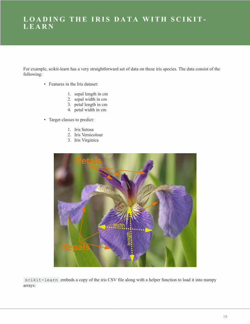
The likelihood that the first dataset you will see in an introductory tutorial on machine learning will be the"Iris dataset" is similarly high. The Iris dataset contains the measurements of 150 iris flowers from 3 differentspecies:
• Iris-Setosa,• Iris-Versicolor, and
15

• Iris-Virginica.
Iris Setosa
Iris Versicolor
Iris Virginica
16

The iris dataset is often used for its simplicity. This dataset is contained in scikit-learn, but before we have adeeper look into the Iris dataset we will look at the other datasets available in scikit-learn.
17
L O A D I N G T H E I R I S D A T A W I T H S C I K I T -L E A R N
For example, scikit-learn has a very straightforward set of data on these iris species. The data consist of thefollowing:
• Features in the Iris dataset:
1. sepal length in cm2. sepal width in cm3. petal length in cm4. petal width in cm
• Target classes to predict:
1. Iris Setosa2. Iris Versicolour3. Iris Virginica
scikit-learn embeds a copy of the iris CSV file along with a helper function to load it into numpyarrays:
18

from sklearn.datasets import load_irisiris = load_iris()
The resulting dataset is a Bunch object:
type(iris)
You can see what's available for this data type by using the method keys() :
iris.keys()
A Bunch object is similar to a dicitionary, but it additionally allows accessing the keys in an attribute style:
print(iris["target_names"])print(iris.target_names)
The features of each sample flower are stored in the data attribute of the dataset:
n_samples, n_features = iris.data.shapeprint('Number of samples:', n_samples)print('Number of features:', n_features)# the sepal length, sepal width, petal length and petal width of the first sample (first flower)print(iris.data[0])
The feautures of each flower are stored in the data attribute of the data set. Let's take a look at some of thesamples:
# Flowers with the indices 12, 26, 89, and 114iris.data[[12, 26, 89, 114]]
Output: sklearn.utils.Bunch
Output: dict_keys(['data', 'target', 'target_names', 'DESCR', 'feature_names', 'filename'])
['setosa' 'versicolor' 'virginica']['setosa' 'versicolor' 'virginica']
Number of samples: 150Number of features: 4[5.1 3.5 1.4 0.2]
19

The information about the class of each sample, i.e. the labels, is stored in the "target" attribute of the data set:
print(iris.data.shape)print(iris.target.shape)
print(iris.target)
import numpy as npnp.bincount(iris.target)
Using NumPy's bincount function (above) we can see that the classes in this dataset are evenly distributed -there are 50 flowers of each species, with
• class 0: Iris Setosa• class 1: Iris Versicolor• class 2: Iris Virginica
These class names are stored in the last attribute, namely target_names :
print(iris.target_names)
Output: array([[4.8, 3. , 1.4, 0.1],[5. , 3.4, 1.6, 0.4],[5.5, 2.5, 4. , 1.3],[5.8, 2.8, 5.1, 2.4]])
(150, 4)(150,)
[0 0 0 0 0 0 0 0 0 0 0 0 0 0 0 0 0 0 0 0 0 0 0 0 0 0 0 0 0 0 0 00 0 0 0 00 0 0 0 0 0 0 0 0 0 0 0 0 1 1 1 1 1 1 1 1 1 1 1 1 1 1 1 1 1 1 1
1 1 1 1 11 1 1 1 1 1 1 1 1 1 1 1 1 1 1 1 1 1 1 1 1 1 1 1 1 1 2 2 2 2 2 2
2 2 2 2 22 2 2 2 2 2 2 2 2 2 2 2 2 2 2 2 2 2 2 2 2 2 2 2 2 2 2 2 2 2 2 2
2 2 2 2 22 2]
Output: array([50, 50, 50])
['setosa' 'versicolor' 'virginica']
20

The information about the class of each sample of our Iris dataset is stored in the target attribute of thedataset:
print(iris.target)
Beside of the shape of the data, we can also check the shape of the labels, i.e. the target.shape :
Each flower sample is one row in the data array, and the columns (features) represent the flower measurementsin centimeters. For instance, we can represent this Iris dataset, consisting of 150 samples and 4 features, a
2-dimensional array or matrix R150 × 4 in the following format:
X = [x ( 1 )
1x ( 1 )
2x ( 1 )
3x ( 1 )
4
x ( 2 )1
x ( 2 )2
x ( 2 )3
x ( 2 )4
� � � �
x ( 150 )1
x ( 150 )2
x ( 150 )3
x ( 150 )4
].
The superscript denotes the ith row, and the subscript denotes the jth feature, respectively.
Generally, we have n rows and k columns:
X = [x ( 1 )
1x ( 1 )
2x ( 1 )
3… x ( 1 )
k
x ( 2 )1
x ( 2 )2
x ( 2 )3
… x ( 2 )k
� � � � �
x ( n )1
x ( n )2
x ( n )3
… x ( n )k
].
print(iris.data.shape)
[0 0 0 0 0 0 0 0 0 0 0 0 0 0 0 0 0 0 0 0 0 0 0 0 0 0 0 0 0 0 0 00 0 0 0 00 0 0 0 0 0 0 0 0 0 0 0 0 1 1 1 1 1 1 1 1 1 1 1 1 1 1 1 1 1 1 1
1 1 1 1 11 1 1 1 1 1 1 1 1 1 1 1 1 1 1 1 1 1 1 1 1 1 1 1 1 1 2 2 2 2 2 2
2 2 2 2 22 2 2 2 2 2 2 2 2 2 2 2 2 2 2 2 2 2 2 2 2 2 2 2 2 2 2 2 2 2 2 2
2 2 2 2 22 2]
21

print(iris.target.shape)
bincount of NumPy counts the number of occurrences of each value in an array of non-negative integers.We can use this to check the distribution of the classes in the dataset:
import numpy as npnp.bincount(iris.target)
We can see that the classes are distributed uniformly - there are 50 flowers from each species, i.e.
• class 0: Iris-Setosa• class 1: Iris-Versicolor• class 2: Iris-Virginica
These class names are stored in the last attribute, namely target_names :
print(iris.target_names)
(150, 4)(150,)
Output: array([50, 50, 50])
['setosa' 'versicolor' 'virginica']
22

V I S U A L I S I N G T H E F E A T U R E S O F T H E I R I SD A T A S E T
The feauture data is four dimensional, but we can visualize one or two of the dimensions at a time using asimple histogram or scatter-plot.
from sklearn.datasets import load_irisiris = load_iris()print(iris.data[iris.target==1][:5])
print(iris.data[iris.target==1, 0][:5])
HISTOGRAMS OF THE FEATURESimport matplotlib.pyplot as pltfig, ax = plt.subplots()x_index = 3colors = ['blue', 'red', 'green']
for label, color in zip(range(len(iris.target_names)), colors):ax.hist(iris.data[iris.target==label, x_index],
label=iris.target_names[label],color=color)
ax.set_xlabel(iris.feature_names[x_index])ax.legend(loc='upper right')fig.show()
[[7. 3.2 4.7 1.4][6.4 3.2 4.5 1.5][6.9 3.1 4.9 1.5][5.5 2.3 4. 1.3][6.5 2.8 4.6 1.5]]
[7. 6.4 6.9 5.5 6.5]
23

EXERCISE
Look at the histograms of the other features, i.e. petal length, sepal widt and sepal length.
SCATTERPLOT WITH TWO FEATURES
The appearance diagram shows two features in one diagram:
import matplotlib.pyplot as pltfig, ax = plt.subplots()
x_index = 3y_index = 0
colors = ['blue', 'red', 'green']
for label, color in zip(range(len(iris.target_names)), colors):ax.scatter(iris.data[iris.target==label, x_index],
iris.data[iris.target==label, y_index],label=iris.target_names[label],c=color)
ax.set_xlabel(iris.feature_names[x_index])ax.set_ylabel(iris.feature_names[y_index])ax.legend(loc='upper left')plt.show()
24

EXERCISE
Change x_index and y_index in the above script
Change x_index and y_index in the above script and find a combination of two parameters which maximallyseparate the three classes.
GENERALIZATION
We will now look at all feature combinations in one combined diagram:
import matplotlib.pyplot as pltn = len(iris.feature_names)fig, ax = plt.subplots(n, n, figsize=(16, 16))
colors = ['blue', 'red', 'green']
for x in range(n):for y in range(n):
xname = iris.feature_names[x]yname = iris.feature_names[y]for color_ind in range(len(iris.target_names)):
ax[x, y].scatter(iris.data[iris.target==color_ind,x],
iris.data[iris.target==color_ind, y],label=iris.target_names[color_ind],c=colors[color_ind])
25

ax[x, y].set_xlabel(xname)ax[x, y].set_ylabel(yname)ax[x, y].legend(loc='upper left')
plt.show()
26

S C A T T E R P L O T ' M A T R I C E S
Instead of doing it manually we can also use the scatterplot matrix provided by the pandas module.
Scatterplot matrices show scatter plots between all features in the data set, as well as histograms to show thedistribution of each feature.
import pandas as pdiris_df = pd.DataFrame(iris.data, columns=iris.feature_names)pd.plotting.scatter_matrix(iris_df,
c=iris.target,figsize=(8, 8)
);
27

3-DIMENSIONAL VISUALIZATIONimport matplotlib.pyplot as pltfrom sklearn.datasets import load_irisfrom mpl_toolkits.mplot3d import Axes3Diris = load_iris()X = []for iclass in range(3):
X.append([[], [], []])for i in range(len(iris.data)):
if iris.target[i] == iclass:X[iclass][0].append(iris.data[i][0])X[iclass][1].append(iris.data[i][1])X[iclass][2].append(sum(iris.data[i][2:]))
colours = ("r", "g", "y")fig = plt.figure()ax = fig.add_subplot(111, projection='3d')
for iclass in range(3):ax.scatter(X[iclass][0], X[iclass][1], X[iclass][2], c=colour
s[iclass])plt.show()
28

D A T A S E T S I N S K L E A R N
Scikit-learn makes available a host ofdatasets for testing learning algorithms.They come in three flavors:
• Packaged Data: these smalldatasets are packaged withthe scikit-learn installation,and can be downloadedusing the tools in
sklearn.datasets.load_*• Downloadable Data: these larger datasets are available for download, and scikit-learn includes
tools which streamline this process. These tools can be found insklearn.datasets.fetch_*
• Generated Data: there are several datasets which are generated from models based on a randomseed. These are available in the sklearn.datasets.make_*
You can explore the available dataset loaders, fetchers, and generators using IPython's tab-completionfunctionality. After importing the datasets submodule from sklearn , type
datasets.load_<TAB>
or
datasets.fetch_<TAB>
or
datasets.make_<TAB>
to see a list of available functions.
STRUCTURE OF DATA AND LABELS
Data in scikit-learn is in most cases saved as two-dimensional Numpy arrays with the shape (n, m) . Manyalgorithms also accept scipy.sparse matrices of the same shape.
29

• n: (n_samples) The number of samples: each sample is an item to process (e.g. classify). Asample can be a document, a picture, a sound, a video, an astronomical object, a row in databaseor CSV file, or whatever you can describe with a fixed set of quantitative traits.
• m: (n_features) The number of features or distinct traits that can be used to describe each item ina quantitative manner. Features are generally real-valued, but may be Boolean or discrete-valuedin some cases.
from sklearn import datasets
Be warned: many of these datasets are quite large, and can take a long time to download!
30

L O A D I N G D I G I T S D A T A
We will have a closer look at one of these datasets. We look at the digits data set. We will load it first:
from sklearn.datasets import load_digitsdigits = load_digits()
Again, we can get an overview of the available attributes by looking at the "keys":
digits.keys()
Let's have a look at the number of items and features:
n_samples, n_features = digits.data.shapeprint((n_samples, n_features))
print(digits.data[0])print(digits.target)
The data is also available at digits.images. This is the raw data of the images in the form of 8 lines and 8columns.
With "data" an image corresponds to a one-dimensional Numpy array with the length 64, and "images"representation contains 2-dimensional numpy arrays with the shape (8, 8)
print("Shape of an item: ", digits.data[0].shape)print("Data type of an item: ", type(digits.data[0]))print("Shape of an item: ", digits.images[0].shape)
Output: dict_keys(['data', 'target', 'target_names', 'images', 'DESCR'])
(1797, 64)
[ 0. 0. 5. 13. 9. 1. 0. 0. 0. 0. 13. 15. 10. 15. 5. 0.0. 3.15. 2. 0. 11. 8. 0. 0. 4. 12. 0. 0. 8. 8. 0. 0. 5.
8. 0.0. 9. 8. 0. 0. 4. 11. 0. 1. 12. 7. 0. 0. 2. 14. 5. 1
0. 12.0. 0. 0. 0. 6. 13. 10. 0. 0. 0.]
[0 1 2 ... 8 9 8]
31

print("Data tpye of an item: ", type(digits.images[0]))
Let's visualize the data. It's little bit more involved than the simple scatter-plot we used above, but we can do itrather quickly.
# set up the figurefig = plt.figure(figsize=(6, 6)) # figure size in inchesfig.subplots_adjust(left=0, right=1, bottom=0, top=1, hspace=0.05, wspace=0.05)
# plot the digits: each image is 8x8 pixelsfor i in range(64):
ax = fig.add_subplot(8, 8, i + 1, xticks=[], yticks=[])ax.imshow(digits.images[i], cmap=plt.cm.binary, interpolatio
n='nearest')
# label the image with the target valueax.text(0, 7, str(digits.target[i]))
Shape of an item: (64,)Data type of an item: <class 'numpy.ndarray'>Shape of an item: (8, 8)Data tpye of an item: <class 'numpy.ndarray'>
32

EXERCISES
EXERCISE 1
sklearn contains a "wine data set".
• Find and load this data set• Can you find a description?• What are the names of the classes?• What are the features?• Where is the data and the labeled data?
EXERCISE 2:
Create a scatter plot of the features ash and color_intensity of the wine data set.
33

EXERCISE 3:
Create a scatter matrix of the features of the wine dataset.
EXERCISE 4:
Fetch the Olivetti faces dataset and visualize the faces.
SOLUTIONS
SOLUTION TO EXERCISE 1
Loading the "wine data set":
from sklearn import datasets
wine = datasets.load_wine()
The description can be accessed via "DESCR":
In [ ]:
print(wine.DESCR)
The names of the classes and the features can be retrieved like this:
print(wine.target_names)print(wine.feature_names)
data = wine.datalabelled_data = wine.target
SOLUTION TO EXERCISE 2:from sklearn import datasetsimport matplotlib.pyplot as plt
['class_0' 'class_1' 'class_2']['alcohol', 'malic_acid', 'ash', 'alcalinity_of_ash', 'magnesium', 'total_phenols', 'flavanoids', 'nonflavanoid_phenols', 'proanthocyanins', 'color_intensity', 'hue', 'od280/od315_of_diluted_wines', 'proline']
34

wine = datasets.load_wine()
features = 'ash', 'color_intensity'features_index = [wine.feature_names.index(features[0]),
wine.feature_names.index(features[1])]
colors = ['blue', 'red', 'green']
for label, color in zip(range(len(wine.target_names)), colors):plt.scatter(wine.data[wine.target==label, features_index[0]],
wine.data[wine.target==label, features_index[1]],label=wine.target_names[label],c=color)
plt.xlabel(features[0])plt.ylabel(features[1])plt.legend(loc='upper left')plt.show()
SOLUTION TO EXERCISE 3:import pandas as pdfrom sklearn import datasets
wine = datasets.load_wine()def rotate_labels(df, axes):
""" changing the rotation of the label output,y labels horizontal and x labels vertical """
35

n = len(df.columns)for x in range(n):
for y in range(n):# to get the axis of subplotsax = axs[x, y]# to make x axis name verticalax.xaxis.label.set_rotation(90)# to make y axis name horizontalax.yaxis.label.set_rotation(0)# to make sure y axis names are outside the plot areaax.yaxis.labelpad = 50
wine_df = pd.DataFrame(wine.data, columns=wine.feature_names)axs = pd.plotting.scatter_matrix(wine_df,
c=wine.target,figsize=(8, 8),
);
rotate_labels(wine_df, axs)
36

SOLUTION TO EXERCISE 4from sklearn.datasets import fetch_olivetti_faces# fetch the faces datafaces = fetch_olivetti_faces()faces.keys()
Output: dict_keys(['data', 'images', 'target', 'DESCR'])
37

n_samples, n_features = faces.data.shapeprint((n_samples, n_features))
np.sqrt(4096)
faces.images.shape
faces.data.shape
print(np.all(faces.images.reshape((400, 4096)) == faces.data))
# set up the figurefig = plt.figure(figsize=(6, 6)) # figure size in inchesfig.subplots_adjust(left=0, right=1, bottom=0, top=1, hspace=0.05, wspace=0.05)
# plot the digits: each image is 8x8 pixelsfor i in range(64):
ax = fig.add_subplot(8, 8, i + 1, xticks=[], yticks=[])ax.imshow(faces.images[i], cmap=plt.cm.bone, interpolation='ne
arest')
# label the image with the target valueax.text(0, 7, str(faces.target[i]))
(400, 4096)
Output: 64.0
Output: (400, 64, 64)
Output: (400, 4096)
True
38

FURTHER DATASETS
sklearn has many more datasets available. If you still need more, you will find more on this nice List ofdatasets for machine-learning research at Wikipedia.
39

D A T A G E N E R A T I O N
GENERATE SYNTHETICAL DATA WITH PYTHON
A problem with machine learning,especially when you are starting out andwant to learn about the algorithms, is thatit is often difficult to get suitable test data.Some cost a lot of money, others are notfreely available because they are protectedby copyright. Therefore, artificiallygenerated test data can be a solution insome cases.
For this reason, this chapter of our tutorialdeals with the artificial generation of data.This chapter is about creating artificialdata. In the previous chapters of ourtutorial we learned that Scikit-Learn(sklearn) contains different data sets. Onthe one hand, there are small toy data sets,but it also offers larger data sets that areoften used in the machine learningcommunity to test algorithms or also serveas a benchmark. It provides us with datacoming from the 'real world'.
All this is great, but in many cases this isstill not sufficient. Maybe you find theright kind of data, but you need more dataof this kind or the data is not completelythe kind of data you were looking for, e.g.maybe you need more complex or lesscomplex data. This is the point where youshould consider to create the datayourself. Here, sklearn offers help. Itincludes various random samplegenerators that can be used to createcustom-made artificial datasets. Datasetsthat meet your ideas of size andcomplexity.
The following Python code is a simple example in which we create artificial weather data for some Germancities. We use Pandas and Numpy to create the data:
import numpy as np
40

import pandas as pd
cities = ['Berlin', 'Frankfurt', 'Hamburg','Nuremberg', 'Munich', 'Stuttgart','Hanover', 'Saarbruecken', 'Cologne','Constance', 'Freiburg', 'Karlsruhe'
]
n= len(cities)data = {'Temperature': np.random.normal(24, 3, n),
'Humidity': np.random.normal(78, 2.5, n),'Wind': np.random.normal(15, 4, n)
}df = pd.DataFrame(data=data, index=cities)df
Output:
Temperature Humidity Wind
Berlin 20.447301 75.516079 12.566956
Frankfurt 27.319526 77.010523 11.800371
Hamburg 24.783113 80.200985 14.489432
Nuremberg 25.823295 76.430166 19.903070
Munich 21.037610 81.589453 17.677132
Stuttgart 25.560423 75.384543 20.832011
Hanover 22.073368 81.704236 12.421998
Saarbruecken 25.722280 80.131432 10.694502
Cologne 25.658240 79.430957 16.360829
Constance 29.221204 75.626223 17.281035
Freiburg 25.625042 81.227281 6.850105
Karlsruhe 26.245587 81.546979 11.787846
41

ANOTHER EXAMPLE
We will create artificial data for four nonexistent types of flowers. If the names remind you of programminglanguages and pizza, it will be no coincidence:
• Flos Pythonem• Flos Java• Flos Margarita• Flos artificialis
The RGB avarage colors values are correspondingly:
• (255, 0, 0)• (245, 107, 0)• (206, 99, 1)• (255, 254, 101)
The average diameter of the calyx is:
• 3.8• 3.3• 4.1• 2.9
Flos pythonem(254, 0, 0)
Flos Java(245, 107, 0)
Flos margarita(206, 99, 1)
Flos artificialis(255, 254, 101)
import matplotlib.pyplot as pltimport numpy as npimport pandas as pdfrom scipy.stats import truncnorm
def truncated_normal(mean=0, sd=1, low=0, upp=10, type=int):return truncnorm(
(low - mean) / sd, (upp - mean) / sd, loc=mean, scale=sd)
def truncated_normal_floats(mean=0, sd=1, low=0, upp=10, num=100):res = truncated_normal(mean=mean, sd=sd, low=low, upp=upp)return res.rvs(num)
def truncated_normal_ints(mean=0, sd=1, low=0, upp=10, num=100):
42

res = truncated_normal(mean=mean, sd=sd, low=low, upp=upp)return res.rvs(num).astype(np.uint8)
# number of items for each flower class:number_of_items_per_class = [190, 205, 230, 170]flowers = {}# flos Pythonem:number_of_items = number_of_items_per_class[0]reds = truncated_normal_ints(mean=254, sd=18, low=235, upp=256,
num=number_of_items)greens = truncated_normal_ints(mean=107, sd=11, low=88, upp=127,
num=number_of_items)blues = truncated_normal_ints(mean=0, sd=15, low=0, upp=20,
num=number_of_items)calyx_dia = truncated_normal_floats(3.8, 0.3, 3.4, 4.2,
num=number_of_items)data = np.column_stack((reds, greens, blues, calyx_dia))flowers["flos_pythonem"] = data
# flos Java:number_of_items = number_of_items_per_class[1]reds = truncated_normal_ints(mean=245, sd=17, low=226, upp=256,
num=number_of_items)greens = truncated_normal_ints(mean=107, sd=11, low=88, upp=127,
num=number_of_items)blues = truncated_normal_ints(mean=0, sd=10, low=0, upp=20,
num=number_of_items)calyx_dia = truncated_normal_floats(3.3, 0.3, 3.0, 3.5,
num=number_of_items)data = np.column_stack((reds, greens, blues, calyx_dia))flowers["flos_java"] = data
# flos Java:number_of_items = number_of_items_per_class[2]reds = truncated_normal_ints(mean=206, sd=17, low=175, upp=238,
num=number_of_items)greens = truncated_normal_ints(mean=99, sd=14, low=80, upp=120,
num=number_of_items)blues = truncated_normal_ints(mean=1, sd=5, low=0, upp=12,
num=number_of_items)calyx_dia = truncated_normal_floats(4.1, 0.3, 3.8, 4.4,
num=number_of_items)data = np.column_stack((reds, greens, blues, calyx_dia))flowers["flos_margarita"] = data
43

# flos artificialis:number_of_items = number_of_items_per_class[3]reds = truncated_normal_ints(mean=255, sd=8, low=2245, upp=2255,
num=number_of_items)greens = truncated_normal_ints(mean=254, sd=10, low=240, upp=255,
num=number_of_items)blues = truncated_normal_ints(mean=101, sd=5, low=90, upp=112,
num=number_of_items)calyx_dia = truncated_normal_floats(2.9, 0.4, 2.4, 3.5,
num=number_of_items)data = np.column_stack((reds, greens, blues, calyx_dia))flowers["flos_artificialis"] = data
data = np.concatenate((flowers["flos_pythonem"],flowers["flos_java"],flowers["flos_margarita"],flowers["flos_artificialis"]
), axis=0)
# assigning the labelstarget = np.zeros(sum(number_of_items_per_class)) # 4 flowersprevious_end = 0for i in range(1, 5):
num = number_of_items_per_class[i-1]beg = previous_endtarget[beg: beg + num] += iprevious_end = beg + num
conc_data = np.concatenate((data, target.reshape(target.shape[0],1)),
axis=1)
np.savetxt("data/strange_flowers.txt", conc_data, fmt="%2.2f",)import matplotlib.pyplot as plttarget_names = list(flowers.keys())feature_names = ['red', 'green', 'blue', 'calyx']n = 4fig, ax = plt.subplots(n, n, figsize=(16, 16))
colors = ['blue', 'red', 'green', 'yellow']
for x in range(n):
44

for y in range(n):xname = feature_names[x]yname = feature_names[y]for color_ind in range(len(target_names)):
ax[x, y].scatter(data[target==color_ind, x],data[target==color_ind, y],label=target_names[color_ind],c=colors[color_ind])
ax[x, y].set_xlabel(xname)ax[x, y].set_ylabel(yname)ax[x, y].legend(loc='upper left')
plt.show()
45

GENERATE SYNTHETIC DATA WITH SCIKIT-LEARN
It is a lot easier to use the possibilities of Scikit-Learn to create synthetic data.
The functionalities available in sklearn can be grouped into
1. Generators for classifictation and clustering2. Generators for creating data for regression3. Generators for manifold learning4. Generators for decomposition
46

GENERATORS FOR CLASSIFICATION AND CLUSTERING
We start with the the function make_blobs of sklearn.datasets to create 'blob' like datadistributions. By setting the value of centers to n_classes , we determine the number of blobs, i.e.the clusters. n_samples corresponds to the total number of points equally divided among clusters. Ifrandom_state is not set, we will have random results every time we call the function. We pass an int to
this parameter for reproducible output across multiple function calls.
import numpy as npimport matplotlib.pyplot as pltfrom sklearn.datasets import make_blobs
n_classes = 4data, labels = make_blobs(n_samples=1000,
centers=n_classes,random_state=100)
labels[:7]
We will visualize the previously created blob custers with matplotlib:
fig, ax = plt.subplots()
colours = ('green', 'orange', 'blue', "pink")for label in range(n_classes):
ax.scatter(x=data[labels==label, 0],y=data[labels==label, 1],c=colours[label],s=40,label=label)
ax.set(xlabel='X',ylabel='Y',title='Blobs Examples')
ax.legend(loc='upper right')
Output: array([1, 3, 1, 3, 1, 3, 2])
47

The centers of the blobs were randomly chosen in the previous example. In the following example we set thecenters of the blobs explicitly. We create a list with the center points and pass it to the parameter centers :
import numpy as npimport matplotlib.pyplot as pltfrom sklearn.datasets import make_blobs
centers = [[2, 3], [4, 5], [7, 9]]data, labels = make_blobs(n_samples=1000,
centers=np.array(centers),random_state=1)
labels[:7]
Let us have a look at the previously created blob clusters:
fig, ax = plt.subplots()
colours = ('green', 'orange', 'blue')for label in range(len(centers)):
ax.scatter(x=data[labels==label, 0],y=data[labels==label, 1],c=colours[label],s=40,
Output: <matplotlib.legend.Legend at 0x7f50f92a4640>
Output: array([0, 1, 1, 0, 2, 2, 2])
48

label=label)
ax.set(xlabel='X',ylabel='Y',title='Blobs Examples')
ax.legend(loc='upper right')
Usually, you want to save your artificially created datasets in a file. For this purpose, we can use the functionsavetxt from numpy. Before we can do this we have to reaarange our data. Each row should contain both
the data and the label:
import numpy as nplabels = labels.reshape((labels.shape[0],1))all_data = np.concatenate((data, labels), axis=1)all_data[:7]
Output: <matplotlib.legend.Legend at 0x7f50f91eaca0>
Output: array([[ 1.72415394, 4.22895559, 0. ],[ 4.16466507, 5.77817418, 1. ],[ 4.51441156, 4.98274913, 1. ],[ 1.49102772, 2.83351405, 0. ],[ 6.0386362 , 7.57298437, 2. ],[ 5.61044976, 9.83428321, 2. ],[ 5.69202866, 10.47239631, 2. ]])
49

For some people it might be complicated to understand the combination of reshape and concatenate.Therefore, you can see an extremely simple example in the following code:
import numpy as npa = np.array( [[1, 2], [3, 4]])b = np.array( [5, 6])b = b.reshape((b.shape[0], 1))print(b)
x = np.concatenate( (a, b), axis=1)x
We use the numpy function savetxt to save the data. Don't worry about the strange name, it is just for funand for reasons which will be clear soon:
np.savetxt("squirrels.txt",all_data,fmt=['%.3f', '%.3f', '%1d'])
all_data[:10]
[[5][6]]
Output: array([[1, 2, 5],[3, 4, 6]])
Output: array([[ 1.72415394, 4.22895559, 0. ],[ 4.16466507, 5.77817418, 1. ],[ 4.51441156, 4.98274913, 1. ],[ 1.49102772, 2.83351405, 0. ],[ 6.0386362 , 7.57298437, 2. ],[ 5.61044976, 9.83428321, 2. ],[ 5.69202866, 10.47239631, 2. ],[ 6.14017298, 8.56209179, 2. ],[ 2.97620068, 5.56776474, 1. ],[ 8.27980017, 8.54824406, 2. ]])
50

R E A D I N G T H E D A T A A N D C O N V E R S I O NB A C K I N T O ' D A T A ' A N D ' L A B E L S '
We will demonstrate now, how to read in the data again and how to split it into data and labels again:
file_data = np.loadtxt("squirrels.txt")
data = file_data[:,:-1]labels = file_data[:,2:]
labels = labels.reshape((labels.shape[0]))
We had called the data file squirrels.txt , because we imagined a strange kind of animal living in theSahara desert. The x-values stand for the night vision capabilities of the animals and the y-values correspondto the colour of the fur, going from sandish to black. We have three kinds of squirrels, 0, 1, and 2. (Be awarethat our squirrals are imaginary squirrels and have nothing to do with the real squirrels of the Sahara!)
import matplotlib.pyplot as pltcolours = ('green', 'red', 'blue', 'magenta', 'yellow', 'cyan')n_classes = 3
fig, ax = plt.subplots()for n_class in range(0, n_classes):
ax.scatter(data[labels==n_class, 0], data[labels==n_class,1],
c=colours[n_class], s=10, label=str(n_class))
ax.set(xlabel='Night Vision',ylabel='Fur color from sandish to black, 0 to 10 ',title='Sahara Virtual Squirrel')
ax.legend(loc='upper right')
51

We will train our articifical data in the following code:
from sklearn.model_selection import train_test_split
data_sets = train_test_split(data,labels,train_size=0.8,test_size=0.2,random_state=42 # garantees same output fo
r every run)
train_data, test_data, train_labels, test_labels = data_sets# import modelfrom sklearn.neighbors import KNeighborsClassifier
# create classifierknn = KNeighborsClassifier(n_neighbors=8)
# trainknn.fit(train_data, train_labels)
# test on test data:calculated_labels = knn.predict(test_data)calculated_labels
Output: <matplotlib.legend.Legend at 0x7f545b4d6340>
52

from sklearn import metrics
print("Accuracy:", metrics.accuracy_score(test_labels, calculated_labels))
Output: array([2., 0., 1., 1., 0., 1., 2., 2., 2., 2., 0., 1., 0.,0., 1., 0., 1.,
2., 0., 0., 1., 2., 1., 2., 2., 1., 2., 0., 0., 2.,0., 2., 2., 0.,
0., 2., 0., 0., 0., 1., 0., 1., 1., 2., 0., 2., 1.,2., 1., 0., 2.,
1., 1., 0., 1., 2., 1., 0., 0., 2., 1., 0., 1., 1.,0., 0., 0., 0.,
0., 0., 0., 1., 1., 0., 1., 1., 1., 0., 1., 2., 1.,2., 0., 2., 1.,
1., 0., 2., 2., 2., 0., 1., 1., 1., 2., 2., 0., 2.,2., 2., 2., 0.,
0., 1., 1., 1., 2., 1., 1., 1., 0., 2., 1., 2., 0.,0., 1., 0., 1.,
0., 2., 2., 2., 1., 1., 1., 0., 2., 1., 2., 2., 1.,2., 0., 2., 0.,
0., 1., 0., 2., 2., 0., 0., 1., 2., 1., 2., 0., 0.,2., 2., 0., 0.,
1., 2., 1., 2., 0., 0., 1., 2., 1., 0., 2., 2., 0.,2., 0., 0., 2.,
1., 0., 0., 0., 0., 2., 2., 1., 0., 2., 2., 1., 2.,0., 1., 1., 1.,
0., 1., 0., 1., 1., 2., 0., 2., 2., 1., 1., 1., 2.])
Accuracy: 0.97
53

O T H E R I N T E R E S T I N G D I S T R I B U T I O N S
import numpy as np
import sklearn.datasets as dsdata, labels = ds.make_moons(n_samples=150,
shuffle=True,noise=0.19,random_state=None)
data += np.array(-np.ndarray.min(data[:,0]),-np.ndarray.min(data[:,1]))
np.ndarray.min(data[:,0]), np.ndarray.min(data[:,1])
import matplotlib.pyplot as pltfig, ax = plt.subplots()
ax.scatter(data[labels==0, 0], data[labels==0, 1],c='orange', s=40, label='oranges')
ax.scatter(data[labels==1, 0], data[labels==1, 1],c='blue', s=40, label='blues')
ax.set(xlabel='X',ylabel='Y',title='Moons')
#ax.legend(loc='upper right');
Output: (0.0, 0.34649342272719386)
54

We want to scale values that are in a range [min, max] in a range [a, b] .
f(x) =(b − a) ⋅ (x − min)
max − min+ a
We now use this formula to transform both the X and Y coordinates of data into other ranges:
min_x_new, max_x_new = 33, 88min_y_new, max_y_new = 12, 20
data, labels = ds.make_moons(n_samples=100,shuffle=True,noise=0.05,random_state=None)
min_x, min_y = np.ndarray.min(data[:,0]), np.ndarray.min(data[:,1])max_x, max_y = np.ndarray.max(data[:,0]), np.ndarray.max(data[:,1])
#data -= np.array([min_x, 0])#data *= np.array([(max_x_new - min_x_new) / (max_x - min_x), 1])#data += np.array([min_x_new, 0])
#data -= np.array([0, min_y])#data *= np.array([1, (max_y_new - min_y_new) / (max_y - min_y)])
Output: [Text(0.5, 0, 'X'), Text(0, 0.5, 'Y'), Text(0.5, 1.0, 'Moons')]
55

#data += np.array([0, min_y_new])
data -= np.array([min_x, min_y])data *= np.array([(max_x_new - min_x_new) / (max_x - min_x), (max_y_new - min_y_new) / (max_y - min_y)])data += np.array([min_x_new, min_y_new])
#np.ndarray.min(data[:,0]), np.ndarray.max(data[:,0])data[:6]
def scale_data(data, new_limits, inplace=False ):if not inplace:
data = data.copy()min_x, min_y = np.ndarray.min(data[:,0]), np.ndarray.min(dat
a[:,1])max_x, max_y = np.ndarray.max(data[:,0]), np.ndarray.max(dat
a[:,1])min_x_new, max_x_new = new_limits[0]min_y_new, max_y_new = new_limits[1]data -= np.array([min_x, min_y])data *= np.array([(max_x_new - min_x_new) / (max_x - min_x),
(max_y_new - min_y_new) / (max_y - min_y)])data += np.array([min_x_new, min_y_new])if inplace:
return Noneelse:
return data
data, labels = ds.make_moons(n_samples=100,shuffle=True,noise=0.05,random_state=None)
scale_data(data, [(1, 4), (3, 8)], inplace=True)
Output: array([[71.14479608, 12.28919998],[62.16584307, 18.75442981],[61.02613211, 12.80794358],[64.30752046, 12.32563839],[81.41469127, 13.64613406],[82.03929032, 13.63156545]])
56

data[:10]
fig, ax = plt.subplots()
ax.scatter(data[labels==0, 0], data[labels==0, 1],c='orange', s=40, label='oranges')
ax.scatter(data[labels==1, 0], data[labels==1, 1],c='blue', s=40, label='blues')
ax.set(xlabel='X',ylabel='Y',title='moons')
ax.legend(loc='upper right');
import sklearn.datasets as dsdata, labels = ds.make_circles(n_samples=100,
shuffle=True,
Output: array([[1.19312571, 6.70797983],[2.74306138, 6.74830445],[1.15255757, 6.31893824],[1.03927303, 4.83714182],[2.91313352, 6.44139267],[2.13227292, 5.120716 ],[2.65590196, 3.49417953],[2.98349928, 5.02232383],[3.35660593, 3.34679462],[2.15813861, 4.8036458 ]])
57

noise=0.05,random_state=None)
fig, ax = plt.subplots()
ax.scatter(data[labels==0, 0], data[labels==0, 1],c='orange', s=40, label='oranges')
ax.scatter(data[labels==1, 0], data[labels==1, 1],c='blue', s=40, label='blues')
ax.set(xlabel='X',ylabel='Y',title='circles')
ax.legend(loc='upper right')
print(__doc__)
import matplotlib.pyplot as pltfrom sklearn.datasets import make_classificationfrom sklearn.datasets import make_blobsfrom sklearn.datasets import make_gaussian_quantiles
plt.figure(figsize=(8, 8))plt.subplots_adjust(bottom=.05, top=.9, left=.05, right=.95)
Output: <matplotlib.legend.Legend at 0x7f54588c2e20>
58

plt.subplot(321)plt.title("One informative feature, one cluster per class", fontsize='small')X1, Y1 = make_classification(n_features=2, n_redundant=0, n_informative=1,
n_clusters_per_class=1)plt.scatter(X1[:, 0], X1[:, 1], marker='o', c=Y1,
s=25, edgecolor='k')
plt.subplot(322)plt.title("Two informative features, one cluster per class", fontsize='small')X1, Y1 = make_classification(n_features=2, n_redundant=0, n_informative=2,
n_clusters_per_class=1)plt.scatter(X1[:, 0], X1[:, 1], marker='o', c=Y1,
s=25, edgecolor='k')
plt.subplot(323)plt.title("Two informative features, two clusters per class",
fontsize='small')X2, Y2 = make_classification(n_features=2,
n_redundant=0,n_informative=2)
plt.scatter(X2[:, 0], X2[:, 1], marker='o', c=Y2,s=25, edgecolor='k')
plt.subplot(324)plt.title("Multi-class, two informative features, one cluster",
fontsize='small')X1, Y1 = make_classification(n_features=2,
n_redundant=0,n_informative=2,n_clusters_per_class=1,n_classes=3)
plt.scatter(X1[:, 0], X1[:, 1], marker='o', c=Y1,s=25, edgecolor='k')
plt.subplot(325)plt.title("Gaussian divided into three quantiles", fontsize='small')X1, Y1 = make_gaussian_quantiles(n_features=2, n_classes=3)plt.scatter(X1[:, 0], X1[:, 1], marker='o', c=Y1,
s=25, edgecolor='k')
59

plt.show()
EXERCISES
EXERCISE 1
Create two testsets which are separable with a perceptron without a bias node.
EXERCISE 2
Create two testsets which are not separable with a dividing line going through the origin.
Automatically created module for IPython interactive environment
60

EXERCISE 3
Create a dataset with five classes "Tiger", "Lion", "Penguin", "Dolphin", and "Python". The sets should looksimilar to the following diagram:
SOLUTIONS
SOLUTION TO EXERCISE 1data, labels = make_blobs(n_samples=100,
cluster_std = 0.5,centers=[[1, 4] ,[4, 1]],random_state=1)
fig, ax = plt.subplots()
colours = ["orange", "green"]label_name = ["Tigers", "Lions"]for label in range(0, 2):
ax.scatter(data[labels==label, 0], data[labels==label, 1],c=colours[label], s=40, label=label_name[label])
ax.set(xlabel='X',ylabel='Y',title='dataset')
61

ax.legend(loc='upper right')
SOLUTION TO EXERCISE 2data, labels = make_blobs(n_samples=100,
cluster_std = 0.5,centers=[[2, 2] ,[4, 4]],random_state=1)
fig, ax = plt.subplots()
colours = ["orange", "green"]label_name = ["label0", "label1"]for label in range(0, 2):
ax.scatter(data[labels==label, 0], data[labels==label, 1],c=colours[label], s=40, label=label_name[label])
ax.set(xlabel='X',ylabel='Y',title='dataset')
ax.legend(loc='upper right')
Output: <matplotlib.legend.Legend at 0x7f788afb2c40>
62

SOLUTION TO EXERCISE 3import sklearn.datasets as dsdata, labels = ds.make_circles(n_samples=100,
shuffle=True,noise=0.05,random_state=42)
centers = [[3, 4], [5, 3], [4.5, 6]]data2, labels2 = make_blobs(n_samples=100,
cluster_std = 0.5,centers=centers,random_state=1)
for i in range(len(centers)-1, -1, -1):labels2[labels2==0+i] = i+2
print(labels2)labels = np.concatenate([labels, labels2])data = data * [1.2, 1.8] + [3, 4]
data = np.concatenate([data, data2], axis=0)
Output: <matplotlib.legend.Legend at 0x7f788af8eac0>
63

fig, ax = plt.subplots()
colours = ["orange", "blue", "magenta", "yellow", "green"]label_name = ["Tiger", "Lion", "Penguin", "Dolphin", "Python"]for label in range(0, len(centers)+2):
ax.scatter(data[labels==label, 0], data[labels==label, 1],c=colours[label], s=40, label=label_name[label])
ax.set(xlabel='X',ylabel='Y',title='dataset')
ax.legend(loc='upper right')
[2 4 4 3 4 4 3 3 2 4 4 2 4 4 3 4 2 4 4 4 4 2 2 4 4 3 2 2 3 2 2 32 3 3 3 33 4 3 3 2 3 3 3 2 2 2 2 3 4 4 4 2 4 3 3 2 2 3 4 4 3 3 4 2 4 2 4
3 3 4 2 23 4 4 2 3 2 3 3 4 2 2 2 2 3 2 4 2 2 3 3 4 4 2 2 4 3]
Output: <matplotlib.legend.Legend at 0x7f788b1d42b0>
64

D A T A P R E P A R A T I O N
LEARN, TEST AND EVALUATION DATA
You have your data ready and you are eager to start training theclassifier? But be careful: When your classifier will be finished,you will need some test data to evaluate your classifier. If youevaluate your classifier with the data used for learning, you maysee surprisingly good results. What we actually want to test isthe performance of classifying on unknown data.
For this purpose, we need to split our data into two parts:
1. A training set with which the learning algorithmadapts or learns the model
2. A test set to evaluate the generalizationperformance of the model
When you consider how machine learning normally works, the idea of a split between learning and test datamakes sense. Really existing systems train on existing data and if other new data (from customers, sensors orother sources) comes in, the trained classifier has to predict or classify this new data. We can simulate thisduring training with a training and test data set - the test data is a simulation of "future data" that will go intothe system during production.
In this chapter of our Python Machine Learning Tutorial, we will learn how to do the splitting with plainPython.
We will see also that doing it manually is not necessary, because the train_test_split function fromthe model_selection module can do it for us.
If the dataset is sorted by label, we will have to shuffle it before splitting.
65

We separated the dataset into a learn (a.k.a. training) dataset and a test dataset. Best practice is to split it into alearn, test and an evaluation dataset.
We will train our model (classifier) step by step and each time the result needs to be tested. If we just have atest dataset. The results of the testing might get into the model. So we will use an evaluation dataset for thecomplete learning phase. When our classifier is finished, we will check it with the test dataset, which it has not"seen" before!
Yet, during our tutorial, we will only use splitings into learn and test datasets.
SPLITTING EXAMPLE: IRIS DATA SET
We will demonstrate the previously discussed topics with the Iris Dataset.
The 150 data sets of the Iris data set are sorted, i.e. the first 50 data correspond to the first flower class (0 =Setosa), the next 50 to the second flower class (1 = Versicolor) and the remaining data correspond to the lastclass (2 = Virginica).
If we were to split our data in the ratio 2/3 (learning set) and 1/3 (test set), the learning set would contain allthe flowers of the first two classes and the test set all the flowers of the third flower class. The classifier couldonly learn two classes and the third class would be completely unknown. So we urgently need to mix the data.
Assuming all samples are independent of each other, we want to shuffle the data set randomly before we splitthe data set as shown above.
66

In the following we split the data manually:
import numpy as npfrom sklearn.datasets import load_irisiris = load_iris()
Looking at the labels of iris.target shows us that the data is sorted.
iris.target
The first thing we have to do is rearrange the data so that it is not sorted anymore. For this purpose, we willuse the permutation function of the random submodul of Numpy:
indices = np.random.permutation(len(iris.data))indices
Output: array([0, 0, 0, 0, 0, 0, 0, 0, 0, 0, 0, 0, 0, 0, 0, 0, 0, 0,0, 0, 0, 0,
0, 0, 0, 0, 0, 0, 0, 0, 0, 0, 0, 0, 0, 0, 0, 0, 0, 0,0, 0, 0, 0,
0, 0, 0, 0, 0, 0, 1, 1, 1, 1, 1, 1, 1, 1, 1, 1, 1, 1,1, 1, 1, 1,
1, 1, 1, 1, 1, 1, 1, 1, 1, 1, 1, 1, 1, 1, 1, 1, 1, 1,1, 1, 1, 1,
1, 1, 1, 1, 1, 1, 1, 1, 1, 1, 1, 1, 2, 2, 2, 2, 2, 2,2, 2, 2, 2,
2, 2, 2, 2, 2, 2, 2, 2, 2, 2, 2, 2, 2, 2, 2, 2, 2, 2,2, 2, 2, 2,
2, 2, 2, 2, 2, 2, 2, 2, 2, 2, 2, 2, 2, 2, 2, 2, 2, 2])
67

n_test_samples = 12learnset_data = iris.data[indices[:-n_test_samples]]learnset_labels = iris.target[indices[:-n_test_samples]]testset_data = iris.data[indices[-n_test_samples:]]testset_labels = iris.target[indices[-n_test_samples:]]print(learnset_data[:4], learnset_labels[:4])print(testset_data[:4], testset_labels[:4])
SPLITS WITH SKLEARN
Even though it was not difficult to split the data manually into a learn (train) and an evaluation (test) set, wedon't have to do the splitting manually as shown above. Since this is often required in machine learning, scikit-learn has a predefined function for dividing data into training and test sets.
Output: array([ 98, 56, 37, 60, 94, 142, 117, 121, 10, 15, 89, 85, 66,
29, 44, 102, 24, 140, 58, 25, 19, 100, 83, 126, 28, 118,
50, 127, 72, 99, 74, 0, 128, 11, 45, 143, 54, 79, 34,
32, 95, 92, 46, 146, 3, 9, 73, 101, 23, 77, 39, 87,
111, 129, 148, 67, 75, 147, 48, 76, 43, 30, 144, 27, 104,
35, 93, 125, 2, 69, 63, 40, 141, 7, 133, 18, 4, 12,
109, 33, 88, 71, 22, 110, 42, 8, 134, 5, 97, 114, 135,
108, 91, 14, 6, 137, 124, 130, 145, 55, 17, 80, 36, 61,
49, 62, 90, 84, 64, 139, 107, 112, 1, 70, 123, 38, 132,
31, 16, 13, 21, 113, 120, 41, 106, 65, 20, 116, 86, 68,
96, 78, 53, 47, 105, 136, 51, 57, 131, 149, 119, 26, 59,
138, 122, 81, 103, 52, 115, 82])
[[5.1 2.5 3. 1.1][6.3 3.3 4.7 1.6][4.9 3.6 1.4 0.1][5. 2. 3.5 1. ]] [1 1 0 1]
[[7.9 3.8 6.4 2. ][5.9 3. 5.1 1.8][6. 2.2 5. 1.5][5. 3.4 1.6 0.4]] [2 2 2 0]
68

We will demonstrate this below. We will use 80% of the data as training and 20% as test data. We could just aswell have taken 70% and 30%, because there are no hard and fast rules. The most important thing is that yourate your system fairly based on data it did not see during exercise! In addition, there must be enough data inboth data sets.
from sklearn.datasets import load_irisfrom sklearn.model_selection import train_test_splitiris = load_iris()data, labels = iris.data, iris.target
res = train_test_split(data, labels,train_size=0.8,test_size=0.2,random_state=42)
train_data, test_data, train_labels, test_labels = res
n = 7print(f"The first {n} data sets:")print(test_data[:7])print(f"The corresponding {n} labels:")print(test_labels[:7])
STRATIFIED RANDOM SAMPLE
Especially with relatively small amounts of data, it is better to stratify the division. Stratification means thatwe keep the original class proportion of the data set in the test and training sets. We calculate the classproportions of the previous split in percent using the following code. To calculate the number of occurrencesof each class, we use the numpy function 'bincount'. It counts the number of occurrences of each value in thearray of non-negative integers passed as an argument.
import numpy as npprint('All:', np.bincount(labels) / float(len(labels)) * 100.0)print('Training:', np.bincount(train_labels) / float(len(train_labels)) * 100.0)
The first 7 data sets:[[6.1 2.8 4.7 1.2][5.7 3.8 1.7 0.3][7.7 2.6 6.9 2.3][6. 2.9 4.5 1.5][6.8 2.8 4.8 1.4][5.4 3.4 1.5 0.4][5.6 2.9 3.6 1.3]]
The corresponding 7 labels:[1 0 2 1 1 0 1]
69

print('Test:', np.bincount(test_labels) / float(len(test_labels))* 100.0)
To stratify the division, we can pass the label array as an additional argument to the train_test_split function:
from sklearn.datasets import load_irisfrom sklearn.model_selection import train_test_splitiris = load_iris()data, labels = iris.data, iris.target
res = train_test_split(data, labels,train_size=0.8,test_size=0.2,random_state=42,stratify=labels)
train_data, test_data, train_labels, test_labels = res
print('All:', np.bincount(labels) / float(len(labels)) * 100.0)print('Training:', np.bincount(train_labels) / float(len(train_labels)) * 100.0)print('Test:', np.bincount(test_labels) / float(len(test_labels))* 100.0)
This was a stupid example to test the stratified random sample, because the Iris data set has the sameproportions, i.e. each class 50 elements.
We will work now with the file strange_flowers.txt of the directory data . This data set is createdin the chapter Generate Datasets in Python The classes in this dataset have different numbers of items. Firstwe load the data:
content = np.loadtxt("data/strange_flowers.txt", delimiter=" ")data = content[:, :-1] # cut of the target columnlabels = content[:, -1]labels.dtypelabels.shape
All: [33.33333333 33.33333333 33.33333333]Training: [33.33333333 34.16666667 32.5 ]Test: [33.33333333 30. 36.66666667]
All: [33.33333333 33.33333333 33.33333333]Training: [33.33333333 33.33333333 33.33333333]Test: [33.33333333 33.33333333 33.33333333]
Output: (795,)
70

res = train_test_split(data, labels,train_size=0.8,test_size=0.2,random_state=42,stratify=labels)
train_data, test_data, train_labels, test_labels = res
# np.bincount expects non negative integers:print('All:', np.bincount(labels.astype(int)) / float(len(labels)) * 100.0)print('Training:', np.bincount(train_labels.astype(int)) / float(len(train_labels)) * 100.0)print('Test:', np.bincount(test_labels.astype(int)) / float(len(test_labels)) * 100.0)All: [ 0. 23.89937107 25.78616352 28.93081761 21.3836478 ]Training: [ 0. 23.89937107 25.78616352 28.93081761 21.3836478 ]Test: [ 0. 23.89937107 25.78616352 28.93081761 21.3836478]
71

K - N E A R E S T - N E I G H B O R C L A S S I F I E R
"Show me who your friends are and I’lltell you who you are?"
The concept of the k-nearest neighborclassifier can hardly be simpler described.This is an old saying, which can be foundin many languages and many cultures. It'salso metnioned in other words in theBible: "He who walks with wise men willbe wise, but the companion of fools willsuffer harm" (Proverbs 13:20 )
This means that the concept of the k-nearest neighbor classifier is part of oureveryday life and judging: Imagine youmeet a group of people, they are all veryyoung, stylish and sportive. They talkabout there friend Ben, who isn't with them. So, what is your imagination of Ben? Right, you imagine him asbeing yong, stylish and sportive as well.
If you learn that Ben lives in a neighborhood where people vote conservative and that the average income isabove 200000 dollars a year? Both his neighbors make even more than 300,000 dollars per year? What do youthink of Ben? Most probably, you do not consider him to be an underdog and you may suspect him to be aconservative as well?
The principle behind nearest neighbor classification consists in finding a predefined number, i.e. the 'k' - oftraining samples closest in distance to a new sample, which has to be classified. The label of the new samplewill be defined from these neighbors. k-nearest neighbor classifiers have a fixed user defined constant for thenumber of neighbors which have to be determined. There are also radius-based neighbor learning algorithms,which have a varying number of neighbors based on the local density of points, all the samples inside of afixed radius. The distance can, in general, be any metric measure: standard Euclidean distance is the mostcommon choice. Neighbors-based methods are known as non-generalizing machine learning methods, sincethey simply "remember" all of its training data. Classification can be computed by a majority vote of thenearest neighbors of the unknown sample.
The k-NN algorithm is among the simplest of all machine learning algorithms, but despite its simplicity, it hasbeen quite successful in a large number of classification and regression problems, for example characterrecognition or image analysis.
Now let's get a little bit more mathematically:
As explained in the chapter Data Preparation, we need labeled learning and test data. In contrast to otherclassifiers, however, the pure nearest-neighbor classifiers do not do any learning, but the so-called learning setLS is a basic component of the classifier. The k-Nearest-Neighbor Classifier (kNN) works directly on thelearned samples, instead of creating rules compared to other classification methods.
72

Nearest Neighbor Algorithm:
Given a set of categories C = {c1, c2, . . . cm}, also called classes, e.g. {"male", "female"}. There is also a
learnset LS consisting of labelled instances:
LS = {(o1, co1), (o2, co2
),⋯(on, con)}
As it makes no sense to have less lebelled items than categories, we can postulate that
n > m and in most cases even n ⋙ m (n much greater than m.)
The task of classification consists in assigning a category or class c to an arbitrary instance o.
For this, we have to differentiate between two cases:
• Case 1:The instance o is an element of LS, i.e. there is a tupel (o, c) ∈ LSIn this case, we will use the class c as the classification result.
• Case 2:We assume now that o is not in LS, or to be precise:∀c ∈ C, (o, c) ∉ LS
o is compared with all the instances of LS. A distance metric d is used for the comparisons.We determine the k closest neighbors of o, i.e. the items with the smallest distances.k is a user defined constant and a positive integer, which is usually small.The number k is typically chosen as the square root of LS, the total number of points in the training data set.
To determine the k nearest neighbors we reorder LS in the following way:(oi1
, coi1
), (oi2, coi2
),⋯(oin, coin
)
so that d(oij, o) ≤ d(oij + 1
, o) is true for all 1 ≤ j ≤ n − 1
The set of k-nearest neighbors Nk consists of the first k elements of this ordering, i.e.
Nk = {(oi1, coi1
), (oi2, coi2
),⋯(oik, coik
)}
The most common class in this set of nearest neighbors Nk will be assigned to the instance o. If there is no
unique most common class, we take an arbitrary one of these.
There is no general way to define an optimal value for 'k'. This value depends on the data. As a general rulewe can say that increasing 'k' reduces the noise but on the other hand makes the boundaries less distinct.
The algorithm for the k-nearest neighbor classifier is among the simplest of all machine learning algorithms.k-NN is a type of instance-based learning, or lazy learning. In machine learning, lazy learning is understoodto be a learning method in which generalization of the training data is delayed until a query is made to thesystem. On the other hand, we have eager learning, where the system usually generalizes the training databefore receiving queries. In other words: The function is only approximated locally and all the computationsare performed, when the actual classification is being performed.
73

The following picture shows in a simple way how the nearest neighbor classifier works. The puzzle piece isunknown. To find out which animal it might be we have to find the neighbors. If k=1 , the only neighbor is acat and we assume in this case that the puzzle piece should be a cat as well. If k=4 , the nearest neighborscontain one chicken and three cats. In this case again, it will be save to assume that our object in questionshould be a cat.
K-NEAREST-NEIGHBOR FROM SCRATCH
PREPARING THE DATASET
Before we actually start with writing a nearest neighbor classifier, we need to think about the data, i.e. thelearnset and the testset. We will use the "iris" dataset provided by the datasets of the sklearn module.
The data set consists of 50 samples from each of three species of Iris
• Iris setosa,• Iris virginica and• Iris versicolor.
Four features were measured from each sample: the length and the width of the sepals and petals, incentimetres.
import numpy as npfrom sklearn import datasets
iris = datasets.load_iris()
74

data = iris.datalabels = iris.target
for i in [0, 79, 99, 101]:print(f"index: {i:3}, features: {data[i]}, label: {label
s[i]}")
We create a learnset from the sets above. We use permutation from np.random to split the datarandomly.
# seeding is only necessary for the website#so that the values are always equal:np.random.seed(42)indices = np.random.permutation(len(data))
n_training_samples = 12learn_data = data[indices[:-n_training_samples]]learn_labels = labels[indices[:-n_training_samples]]test_data = data[indices[-n_training_samples:]]test_labels = labels[indices[-n_training_samples:]]
print("The first samples of our learn set:")print(f"{'index':7s}{'data':20s}{'label':3s}")for i in range(5):
print(f"{i:4d} {learn_data[i]} {learn_labels[i]:3}")print("The first samples of our test set:")print(f"{'index':7s}{'data':20s}{'label':3s}")for i in range(5):
print(f"{i:4d} {learn_data[i]} {learn_labels[i]:3}")
index: 0, features: [5.1 3.5 1.4 0.2], label: 0index: 79, features: [5.7 2.6 3.5 1. ], label: 1index: 99, features: [5.7 2.8 4.1 1.3], label: 1index: 101, features: [5.8 2.7 5.1 1.9], label: 2
75

The following code is only necessary to visualize the data of our learnset. Our data consists of four values periris item, so we will reduce the data to three values by summing up the third and fourth value. This way, weare capable of depicting the data in 3-dimensional space:
#%matplotlib widget
import matplotlib.pyplot as pltfrom mpl_toolkits.mplot3d import Axes3D
colours = ("r", "b")X = []for iclass in range(3):
X.append([[], [], []])for i in range(len(learn_data)):
if learn_labels[i] == iclass:X[iclass][0].append(learn_data[i][0])X[iclass][1].append(learn_data[i][1])X[iclass][2].append(sum(learn_data[i][2:]))
colours = ("r", "g", "y")
fig = plt.figure()ax = fig.add_subplot(111, projection='3d')
for iclass in range(3):ax.scatter(X[iclass][0], X[iclass][1], X[iclass][2], c=colo
urs[iclass])plt.show()
The first samples of our learn set:index data label
0 [6.1 2.8 4.7 1.2] 11 [5.7 3.8 1.7 0.3] 02 [7.7 2.6 6.9 2.3] 23 [6. 2.9 4.5 1.5] 14 [6.8 2.8 4.8 1.4] 1
The first samples of our test set:index data label
0 [6.1 2.8 4.7 1.2] 11 [5.7 3.8 1.7 0.3] 02 [7.7 2.6 6.9 2.3] 23 [6. 2.9 4.5 1.5] 14 [6.8 2.8 4.8 1.4] 1
76

DISTANCE METRICS
We have already mentioned in detail, we calculate the distances between the points of the sample and theobject to be classified. To calculate these distances we need a distance function.
In n-dimensional vector rooms, one usually uses one of the following three distance metrics:
• Euclidean Distance
The Euclidean distance between two points x and y in either the plane or 3-dimensionalspace measures the length of a line segment connecting these two points. It can be calculatedfrom the Cartesian coordinates of the points using the Pythagorean theorem, therefore it is alsooccasionally being called the Pythagorean distance. The general formula is
d(x, y) = √n
∑i = 1
(xi − yi)2
• Manhattan Distance
It is defined as the sum of the absolute values of the differences between the coordinates of xand y:
d(x, y) =
n
∑i = 1
| xi − yi |
• Minkowski Distance
The Minkowski distance generalizes the Euclidean and the Manhatten distance in one distancemetric. If we set the parameter p in the following formula to 1 we get the manhattan distancean using the value 2 gives us the euclidean distance:
77

d(x, y) = (n
∑i = 1
| xi − yi | p)1
p
The following diagram visualises the Euclidean and the Manhattan distance:
The blue line illustrates the Eucliden distance between the green and red dot. Otherwise you can also moveover the orange, green or yellow line from the green point to the red point. The lines correspond to themanhatten distance. The length is equal.
DETERMINING THE NEIGHBORS
To determine the similarity between two instances, we will use the Euclidean distance.
We can calculate the Euclidean distance with the function norm of the module np.linalg :
def distance(instance1, instance2):""" Calculates the Eucledian distance between two instance
s"""return np.linalg.norm(np.subtract(instance1, instance2))
print(distance([3, 5], [1, 1]))print(distance(learn_data[3], learn_data[44]))
78

The function get_neighbors returns a list with k neighbors, which are closest to the instancetest_instance :
def get_neighbors(training_set,labels,test_instance,k,distance):
"""get_neighors calculates a list of the k nearest neighborsof an instance 'test_instance'.The function returns a list of k 3-tuples.Each 3-tuples consists of (index, dist, label)whereindex is the index from the training_set,dist is the distance between the test_instance and the
instance training_set[index]distance is a reference to a function used to calculate the
distances"""distances = []for index in range(len(training_set)):
dist = distance(test_instance, training_set[index])distances.append((training_set[index], dist, labels[inde
x]))distances.sort(key=lambda x: x[1])neighbors = distances[:k]return neighbors
We will test the function with our iris samples:
for i in range(5):neighbors = get_neighbors(learn_data,
learn_labels,test_data[i],3,distance=distance)
print("Index: ",i,'\n',"Testset Data: ",test_data[i],'\n',"Testset Label: ",test_labels[i],'\n',"Neighbors: ",neighbors,'\n')
4.472135954999583.4190641994557516
79

VOTING TO GET A SINGLE RESULT
We will write a vote function now. This functions uses the class Counter from collections to countthe quantity of the classes inside of an instance list. This instance list will be the neighbors of course. Thefunction vote returns the most common class:
from collections import Counter
def vote(neighbors):
Index: 0Testset Data: [5.7 2.8 4.1 1.3]Testset Label: 1Neighbors: [(array([5.7, 2.9, 4.2, 1.3]), 0.141421356237309
95, 1), (array([5.6, 2.7, 4.2, 1.3]), 0.17320508075688815, 1), (array([5.6, 3. , 4.1, 1.3]), 0.22360679774997935, 1)]
Index: 1Testset Data: [6.5 3. 5.5 1.8]Testset Label: 2Neighbors: [(array([6.4, 3.1, 5.5, 1.8]), 0.141421356237309
3, 2), (array([6.3, 2.9, 5.6, 1.8]), 0.24494897427831783, 2), (array([6.5, 3. , 5.2, 2. ]), 0.3605551275463988, 2)]
Index: 2Testset Data: [6.3 2.3 4.4 1.3]Testset Label: 1Neighbors: [(array([6.2, 2.2, 4.5, 1.5]), 0.264575131106458
6, 1), (array([6.3, 2.5, 4.9, 1.5]), 0.574456264653803, 1), (array([6. , 2.2, 4. , 1. ]), 0.5916079783099617, 1)]
Index: 3Testset Data: [6.4 2.9 4.3 1.3]Testset Label: 1Neighbors: [(array([6.2, 2.9, 4.3, 1.3]), 0.200000000000000
18, 1), (array([6.6, 3. , 4.4, 1.4]), 0.2645751311064587, 1), (array([6.6, 2.9, 4.6, 1.3]), 0.3605551275463984, 1)]
Index: 4Testset Data: [5.6 2.8 4.9 2. ]Testset Label: 2Neighbors: [(array([5.8, 2.7, 5.1, 1.9]), 0.316227766016837
5, 2), (array([5.8, 2.7, 5.1, 1.9]), 0.3162277660168375, 2), (array([5.7, 2.5, 5. , 2. ]), 0.33166247903553986, 2)]
80

class_counter = Counter()for neighbor in neighbors:
class_counter[neighbor[2]] += 1return class_counter.most_common(1)[0][0]
We will test 'vote' on our training samples:
for i in range(n_training_samples):neighbors = get_neighbors(learn_data,
learn_labels,test_data[i],3,distance=distance)
print("index: ", i,", result of vote: ", vote(neighbors),", label: ", test_labels[i],", data: ", test_data[i])
We can see that the predictions correspond to the labelled results, except in case of the item with the index 8.
index: 0 , result of vote: 1 , label: 1 , data: [5.7 2.8 4.11.3]index: 1 , result of vote: 2 , label: 2 , data: [6.5 3. 5.51.8]index: 2 , result of vote: 1 , label: 1 , data: [6.3 2.3 4.41.3]index: 3 , result of vote: 1 , label: 1 , data: [6.4 2.9 4.31.3]index: 4 , result of vote: 2 , label: 2 , data: [5.6 2.8 4.92. ]index: 5 , result of vote: 2 , label: 2 , data: [5.9 3. 5.11.8]index: 6 , result of vote: 0 , label: 0 , data: [5.4 3.4 1.70.2]index: 7 , result of vote: 1 , label: 1 , data: [6.1 2.8 4.1.3]index: 8 , result of vote: 1 , label: 2 , data: [4.9 2.5 4.51.7]index: 9 , result of vote: 0 , label: 0 , data: [5.8 4. 1.20.2]index: 10 , result of vote: 1 , label: 1 , data: [5.8 2.6 4.1.2]index: 11 , result of vote: 2 , label: 2 , data: [7.1 3. 5.92.1]
81

'vote_prob' is a function like 'vote' but returns the class name and the probability for this class:
def vote_prob(neighbors):class_counter = Counter()for neighbor in neighbors:
class_counter[neighbor[2]] += 1labels, votes = zip(*class_counter.most_common())winner = class_counter.most_common(1)[0][0]votes4winner = class_counter.most_common(1)[0][1]return winner, votes4winner/sum(votes)
for i in range(n_training_samples):neighbors = get_neighbors(learn_data,
learn_labels,test_data[i],5,distance=distance)
print("index: ", i,", vote_prob: ", vote_prob(neighbors),", label: ", test_labels[i],", data: ", test_data[i])
82

THE WEIGHTED NEAREST NEIGHBOUR CLASSIFIER
We looked only at k items in the vicinity of an unknown object „UO", and had a majority vote. Using themajority vote has shown quite efficient in our previous example, but this didn't take into account the followingreasoning: The farther a neighbor is, the more it "deviates" from the "real" result. Or in other words, we cantrust the closest neighbors more than the farther ones. Let's assume, we have 11 neighbors of an unknown itemUO. The closest five neighbors belong to a class A and all the other six, which are farther away belong to aclass B. What class should be assigned to UO? The previous approach says B, because we have a 6 to 5 votein favor of B. On the other hand the closest 5 are all A and this should count more.
To pursue this strategy, we can assign weights to the neighbors in the following way: The nearest neighbor ofan instance gets a weight 1 /1, the second closest gets a weight of 1 /2 and then going on up to 1 /k for thefarthest away neighbor.
This means that we are using the harmonic series as weights:
k
∑i
1/ (i + 1) = 1 +1
2+
1
3+ . . . +
1
k
We implement this in the following function:
index: 0 , vote_prob: (1, 1.0) , label: 1 , data: [5.7 2.84.1 1.3]index: 1 , vote_prob: (2, 1.0) , label: 2 , data: [6.5 3.5.5 1.8]index: 2 , vote_prob: (1, 1.0) , label: 1 , data: [6.3 2.34.4 1.3]index: 3 , vote_prob: (1, 1.0) , label: 1 , data: [6.4 2.94.3 1.3]index: 4 , vote_prob: (2, 1.0) , label: 2 , data: [5.6 2.84.9 2. ]index: 5 , vote_prob: (2, 0.8) , label: 2 , data: [5.9 3.5.1 1.8]index: 6 , vote_prob: (0, 1.0) , label: 0 , data: [5.4 3.41.7 0.2]index: 7 , vote_prob: (1, 1.0) , label: 1 , data: [6.1 2.84. 1.3]index: 8 , vote_prob: (1, 1.0) , label: 2 , data: [4.9 2.54.5 1.7]index: 9 , vote_prob: (0, 1.0) , label: 0 , data: [5.8 4.1.2 0.2]index: 10 , vote_prob: (1, 1.0) , label: 1 , data: [5.8 2.64. 1.2]index: 11 , vote_prob: (2, 1.0) , label: 2 , data: [7.1 3.5.9 2.1]
83

def vote_harmonic_weights(neighbors, all_results=True):class_counter = Counter()number_of_neighbors = len(neighbors)for index in range(number_of_neighbors):
class_counter[neighbors[index][2]] += 1/(index+1)labels, votes = zip(*class_counter.most_common())#print(labels, votes)winner = class_counter.most_common(1)[0][0]votes4winner = class_counter.most_common(1)[0][1]if all_results:
total = sum(class_counter.values(), 0.0)for key in class_counter:
class_counter[key] /= totalreturn winner, class_counter.most_common()
else:return winner, votes4winner / sum(votes)
for i in range(n_training_samples):neighbors = get_neighbors(learn_data,
learn_labels,test_data[i],6,distance=distance)
print("index: ", i,", result of vote: ",vote_harmonic_weights(neighbors,
all_results=True))
The previous approach took only the ranking of the neighbors according to their distance in account. We can
index: 0 , result of vote: (1, [(1, 1.0)])index: 1 , result of vote: (2, [(2, 1.0)])index: 2 , result of vote: (1, [(1, 1.0)])index: 3 , result of vote: (1, [(1, 1.0)])index: 4 , result of vote: (2, [(2, 0.9319727891156463), (1, 0.06802721088435375)])index: 5 , result of vote: (2, [(2, 0.8503401360544217), (1, 0.14965986394557826)])index: 6 , result of vote: (0, [(0, 1.0)])index: 7 , result of vote: (1, [(1, 1.0)])index: 8 , result of vote: (1, [(1, 1.0)])index: 9 , result of vote: (0, [(0, 1.0)])index: 10 , result of vote: (1, [(1, 1.0)])index: 11 , result of vote: (2, [(2, 1.0)])
84

improve the voting by using the actual distance. To this purpos we will write a new voting function:
def vote_distance_weights(neighbors, all_results=True):class_counter = Counter()number_of_neighbors = len(neighbors)for index in range(number_of_neighbors):
dist = neighbors[index][1]label = neighbors[index][2]class_counter[label] += 1 / (dist**2 + 1)
labels, votes = zip(*class_counter.most_common())#print(labels, votes)winner = class_counter.most_common(1)[0][0]votes4winner = class_counter.most_common(1)[0][1]if all_results:
total = sum(class_counter.values(), 0.0)for key in class_counter:
class_counter[key] /= totalreturn winner, class_counter.most_common()
else:return winner, votes4winner / sum(votes)
for i in range(n_training_samples):neighbors = get_neighbors(learn_data,
learn_labels,test_data[i],6,distance=distance)
print("index: ", i,", result of vote: ",vote_distance_weights(neighbors,
all_results=True))
85

ANOTHER EXAMPLE FOR NEAREST NEIGHBOR CLASSIFICATION
We want to test the previous functions with another very simple dataset:
train_set = [(1, 2, 2),(-3, -2, 0),(1, 1, 3),(-3, -3, -1),(-3, -2, -0.5),(0, 0.3, 0.8),(-0.5, 0.6, 0.7),(0, 0, 0)
]
labels = ['apple', 'banana', 'apple','banana', 'apple', "orange",'orange', 'orange']
k = 2for test_instance in [(0, 0, 0), (2, 2, 2),
(-3, -1, 0), (0, 1, 0.9),(1, 1.5, 1.8), (0.9, 0.8, 1.6)]:
neighbors = get_neighbors(train_set,labels,test_instance,k,distance=distance)
print("vote distance weights: ",vote_distance_weights(neighbors))
index: 0 , result of vote: (1, [(1, 1.0)])index: 1 , result of vote: (2, [(2, 1.0)])index: 2 , result of vote: (1, [(1, 1.0)])index: 3 , result of vote: (1, [(1, 1.0)])index: 4 , result of vote: (2, [(2, 0.8490154592118361), (1, 0.15098454078816387)])index: 5 , result of vote: (2, [(2, 0.6736137462184478), (1, 0.3263862537815521)])index: 6 , result of vote: (0, [(0, 1.0)])index: 7 , result of vote: (1, [(1, 1.0)])index: 8 , result of vote: (1, [(1, 1.0)])index: 9 , result of vote: (0, [(0, 1.0)])index: 10 , result of vote: (1, [(1, 1.0)])index: 11 , result of vote: (2, [(2, 1.0)])
86

KNN IN LINGUISTICS
The next example comes from computer linguistics. We show how we can use a k-nearest neighbor classifierto recognize misspelled words.
We use a module called levenshtein, which we have implemented in our tutorial on Levenshtein Distance.
from levenshtein import levenshtein
cities = open("data/city_names.txt").readlines()cities = [city.strip() for city in cities]
for city in ["Freiburg", "Frieburg", "Freiborg","Hamborg", "Sahrluis"]:
neighbors = get_neighbors(cities,cities,city,2,distance=levenshtein)
print("vote_distance_weights: ", vote_distance_weights(neighbors))
Marvin and James introduce us to our next example:
vote distance weights: ('orange', [('orange', 1.0)])vote distance weights: ('apple', [('apple', 1.0)])vote distance weights: ('banana', [('banana', 0.5294117647058824), ('apple', 0.47058823529411764)])vote distance weights: ('orange', [('orange', 1.0)])vote distance weights: ('apple', [('apple', 1.0)])vote distance weights: ('apple', [('apple', 0.5084745762711865),('orange', 0.4915254237288135)])
vote_distance_weights: ('Freiberg', [('Freiberg', 0.8333333333333334), ('Freising', 0.16666666666666669)])vote_distance_weights: ('Lüneburg', [('Lüneburg', 0.5), ('Duisburg', 0.5)])vote_distance_weights: ('Freiberg', [('Freiberg', 0.8333333333333334), ('Freising', 0.16666666666666669)])vote_distance_weights: ('Hamburg', [('Hamburg', 0.7142857142857143), ('Bamberg', 0.28571428571428575)])vote_distance_weights: ('Saarlouis', [('Saarlouis', 0.8387096774193549), ('Bayreuth', 0.16129032258064516)])
87

Can you help Marvin and James?
88

british-english.txt
You will need an English dictionary and a k-nearest Neighbor classifier to solve this problem. If you workunder Linux (especially Ubuntu), you can find a file with a British-English dictionary under /usr/share/dict/british-english. Windows users and others can download the file as
We use extremely misspelled words in the following example. We see that our simple vote_prob function isdoing well only in two cases: In correcting "holpposs" to "helpless" and "blagrufoo" to "barefoot". Whereasour distance voting is doing well in all cases. Okay, we have to admit that we had "liberty" in mind, when wewrote "liberdi", but suggesting "liberal" is a good choice.
words = []with open("british-english.txt") as fh:
for line in fh:word = line.strip()words.append(word)
89

for word in ["holpful", "kundnoss", "holpposs", "thoes", "innerstand",
"blagrufoo", "liberdi"]:neighbors = get_neighbors(words,
words,word,3,distance=levenshtein)
print("vote_distance_weights: ", vote_distance_weights(neighbors,
all_results=False))
print("vote_prob: ", vote_prob(neighbors))print("vote_distance_weights: ", vote_distance_weights(neighbo
rs))
90

vote_distance_weights: ('helpful', 0.5555555555555556)vote_prob: ('helpful', 0.3333333333333333)vote_distance_weights: ('helpful', [('helpful', 0.5555555555555556), ('doleful', 0.22222222222222227), ('hopeful', 0.22222222222222227)])vote_distance_weights: ('kindness', 0.5)vote_prob: ('kindness', 0.3333333333333333)vote_distance_weights: ('kindness', [('kindness', 0.5), ('fondness', 0.25), ('kudos', 0.25)])vote_distance_weights: ('helpless', 0.3333333333333333)vote_prob: ('helpless', 0.3333333333333333)vote_distance_weights: ('helpless', [('helpless', 0.3333333333333333), ("hippo's", 0.3333333333333333), ('hippos', 0.3333333333333333)])vote_distance_weights: ('hoes', 0.3333333333333333)vote_prob: ('hoes', 0.3333333333333333)vote_distance_weights: ('hoes', [('hoes', 0.3333333333333333),('shoes', 0.3333333333333333), ('thees', 0.3333333333333333)])vote_distance_weights: ('understand', 0.5)vote_prob: ('understand', 0.3333333333333333)vote_distance_weights: ('understand', [('understand', 0.5), ('interstate', 0.25), ('understands', 0.25)])vote_distance_weights: ('barefoot', 0.4333333333333333)vote_prob: ('barefoot', 0.3333333333333333)vote_distance_weights: ('barefoot', [('barefoot', 0.4333333333333333), ('Baguio', 0.2833333333333333), ('Blackfoot', 0.2833333333333333)])vote_distance_weights: ('liberal', 0.4)vote_prob: ('liberal', 0.3333333333333333)vote_distance_weights: ('liberal', [('liberal', 0.4), ('liberty', 0.4), ('Hibernia', 0.2)])
91

N E U R A L N E T W O R K S
INTRODUCTION
When we say "Neural Networks", wemean artificial Neural Networks (ANN).The idea of ANN is based on biologicalneural networks like the brain of livingbeing.
The basic structure of a neural network -both an artificial and a living one - is theneuron. A neuron in biology consists ofthree major parts: the soma (cell body),the dendrites and the axon.
The dendrites branch of from the soma ina tree-like way and become thinner withevery branch. They receive signals(impulses) from other neurons at synapses. The axon - there is always only one - also leaves the soma andusually tend to extend for longer distances than the dentrites. The axon is used for sending the output of theneuron to other neurons or better to the synapsis of other neurons.
BIOLOGICAL NEURON
The following image by Quasar Jarosz, courtesy of Wikipedia, illustrates this:
92

ABSTRACTION OF A BIOLOGICAL NEURON AND ARTIFICIAL NEURON
Even though the above image is already an abstraction for a biologist, we can further abstract it:
A perceptron of artificial neural networks is simulating a biological neuron.
It is amazingly simple, what is going on inside the body of a perceptron or neuron. The input signals getmultiplied by weight values, i.e. each input has its corresponding weight. This way the input can be adjustedindividually for every xi. We can see all the inputs as an input vector and the corresponding weights as the
weights vector.
When a signal comes in, it gets multiplied by a weight value that is assigned to this particular input. That is, ifa neuron has three inputs, then it has three weights that can be adjusted individually. The weights usually getadjusted during the learn phase.After this the modified input signals are summed up. It is also possible to add additionally a so-called bias 'b'to this sum. The bias is a value which can also be adjusted during the learn phase.
Finally, the actual output has to be determined. For this purpose an activation or step function Φ is applied tothe weighted sum of the input values.
93

The simplest form of an activation function is a binary function. If the result of the summation is greater thansome threshold s, the result of Φ will be 1, otherwise 0.
Φ(x) = {1 wx + b > s
0 otherwise
NUMBER OF NEURON IN ANIMALS
We will examine in the following chapters artificial neuronal networks of various sizes and structures. It isinteresting to have a look at the total numbers of neurons some animals have:
• Roundworm: 302• Jellyfish
94

In [ ]:
95

F R O M D I V I D I N G L I N E S T O N E U R A LN E T W O R K S
We will develop a simple neural network in this chapter of our tutorial. A network capable of separating twoclasses, which are separable by a straight line in a 2-dimensional feature space.
LINE SEPARATION
Before we start programming a simple neuralnetwork, we are going to develop a different concept.We want to search for straight lines that separate twopoints or two classes in a plane. We will only look atstraight lines going through the origin. We will lookat general straight lines later in the tutorial.
You could imagine that you have two attributesdescribing an eddible object like a fruit for example:"sweetness" and "sourness".
We could describe this by points in a two-dimensional space. The A axis is used for the valuesof sweetness and the y axis is correspondingly usedfor the sourness values. Imagine now that we havetwo fruits as points in this space, i.e. an orange atposition (3.5, 1.8) and a lemon at (1.1, 3.9).
We could define dividing lines to define the points which are more lemon-like and which are more orange-like.
In the following diagram, we depict one lemon and one orange. The green line is separating both points. Weassume that all other lemons are above this line and all oranges will be below this line.
96

The green line is defined by
y = mx
where:
m is the slope or gradient of the line and x is the independent variable of the function.
m =p2
p1x
This means that a point P ′ = (p ′1, p ′
2) is on this line, if the following condition is fulfilled:
mp ′1
− p ′2
= 0
The following Python program plots a graph depicting the previously described situation:
import matplotlib.pyplot as pltimport numpy as np
97

X = np.arange(0, 7)fig, ax = plt.subplots()
ax.plot(3.5, 1.8, "or",color="darkorange",markersize=15)
ax.plot(1.1, 3.9, "oy",markersize=15)
point_on_line = (4, 4.5)ax.plot(1.1, 3.9, "oy", markersize=15)# calculate gradient:m = point_on_line[1] / point_on_line[0]ax.plot(X, m * X, "g-", linewidth=3)plt.show()
It is clear that a point A = (a1, a2) is not on the line, if m ⋅ a1 − a2 is not equal to 0. We want to know more.
We want to know, if a point is above or below a straight line.
98

If a point B = (b1, b2) is below this line, there must be a δB > 0 so that the point (b1, b2 + δB) will be on the
line.
This means that
m ⋅ b1 − (b2 + δB) = 0
which can be rearranged to
m ⋅ b1 − b2 = δB
Finally, we have a criteria for a point to be below the line. m ⋅ b1 − b2 is positve, because δB is positive.
The reasoning for "a point is above the line" is analogue: If a point A = (a1, a2) is above the line, there must
be a δA > 0 so that the point (a1, a2 − δA) will be on the line.
This means that
m ⋅ a1 − (a2 − δA) = 0
which can be rearranged to
m ⋅ a1 − a2 = − δA
99

In summary, we can say: A point P(p1, p2) lies
• below the straight line if m ⋅ p1 − p2 > 0
• on the straight line if m ⋅ p1 − p2 = 0
• above the straight line if m ⋅ p1 − p2 < 0
We can now verify this on our fruits. The lemon has the coordinates (1.1, 3.9) and the orange the coordinates3.5, 1.8. The point on the line, which we used to define our separation straight line has the values (4, 4.5). Som is 4.5 divides by 4.
lemon = (1.1, 3.9)orange = (3.5, 1.8)m = 4.5 / 4
# check if orange is below the line,# positive value is expected:print(orange[0] * m - orange[1])
# check if lemon is above the line,# negative value is expected:print(lemon[0] * m - lemon[1])
We did not calculate the green line using mathematical formulas or methods, but arbitrarily determined it byvisual judgement. We could have chosen other lines as well.
The following Python program calculates and renders a bunch of lines. All going through the origin, i.e. thepoint (0, 0). The red ones are completely unusable for the purpose of separating the two fruits, because inthese cases both the lemon and the orange are on the same side of the straight line. However, it is obvious thateven the green ones might not be too useful if we have more than these two fruits. Some lemons might besweeter and some oranges can be quite sour.
import numpy as npimport matplotlib.pyplot as pltdef create_distance_function(a, b, c):
""" 0 = ax + by + c """def distance(x, y):
"""returns tuple (d, pos)d is the distance
2.1375-2.6624999999999996
100

If pos == -1 point is below the line,0 on the line and +1 if above the line"""nom = a * x + b * y + cif nom == 0:
pos = 0elif (nom<0 and b<0) or (nom>0 and b>0):
pos = -1else:
pos = 1return (np.absolute(nom) / np.sqrt( a ** 2 + b ** 2), pos)
return distance
orange = (4.5, 1.8)lemon = (1.1, 3.9)fruits_coords = [orange, lemon]
fig, ax = plt.subplots()ax.set_xlabel("sweetness")ax.set_ylabel("sourness")x_min, x_max = -1, 7y_min, y_max = -1, 8ax.set_xlim([x_min, x_max])ax.set_ylim([y_min, y_max])X = np.arange(x_min, x_max, 0.1)
step = 0.05for x in np.arange(0, 1+step, step):
slope = np.tan(np.arccos(x))dist4line1 = create_distance_function(slope, -1, 0)Y = slope * Xresults = []for point in fruits_coords:
results.append(dist4line1(*point))if (results[0][1] != results[1][1]):
ax.plot(X, Y, "g-", linewidth=0.8, alpha=0.9)else:
ax.plot(X, Y, "r-", linewidth=0.8, alpha=0.9)
size = 10for (index, (x, y)) in enumerate(fruits_coords):
if index== 0:ax.plot(x, y, "o",
color="darkorange",markersize=size)
101

else:ax.plot(x, y, "oy",
markersize=size)
plt.show()
Basically, we have carried out a classification based on our dividing line. Even if hardly anyone woulddescribe this as such.
It is easy to imagine that we have more lemons and oranges with slightly different sourness and sweetnessvalues. This means we have a class of lemons ( class1 ) and a class of oranges class2 . This is depictedin the following diagram.
102

We are going to "grow" oranges and lemons with a Python program. We will create these two classes byrandomly creating points within a circle with a defined center point and radius. The following Python codewill create the classes:
import numpy as npimport matplotlib.pyplot as pltdef points_within_circle(radius,
center=(0, 0),number_of_points=100):
center_x, center_y = centerr = radius * np.sqrt(np.random.random((number_of_points,)))theta = np.random.random((number_of_points,)) * 2 * np.pix = center_x + r * np.cos(theta)y = center_y + r * np.sin(theta)return x, y
X = np.arange(0, 8)fig, ax = plt.subplots()oranges_x, oranges_y = points_within_circle(1.6, (5, 2), 100)lemons_x, lemons_y = points_within_circle(1.9, (2, 5), 100)
ax.scatter(oranges_x,oranges_y,c="orange",label="oranges")
ax.scatter(lemons_x,
103
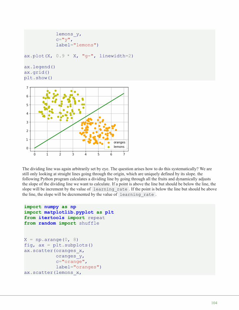
lemons_y,c="y",label="lemons")
ax.plot(X, 0.9 * X, "g-", linewidth=2)
ax.legend()ax.grid()plt.show()
The dividing line was again arbitrarily set by eye. The question arises how to do this systematically? We arestill only looking at straight lines going through the origin, which are uniquely defined by its slope. thefollowing Python program calculates a dividing line by going through all the fruits and dynamically adjuststhe slope of the dividing line we want to calculate. If a point is above the line but should be below the line, theslope will be increment by the value of learning_rate . If the point is below the line but should be abovethe line, the slope will be decremented by the value of learning_rate .
import numpy as npimport matplotlib.pyplot as pltfrom itertools import repeatfrom random import shuffle
X = np.arange(0, 8)fig, ax = plt.subplots()ax.scatter(oranges_x,
oranges_y,c="orange",label="oranges")
ax.scatter(lemons_x,
104

lemons_y,c="y",label="lemons")
fruits = list(zip(oranges_x,oranges_y,repeat(0, len(oranges_x))))
fruits += list(zip(lemons_x,lemons_y,repeat(1, len(oranges_x))))
shuffle(fruits)
def adjust(learning_rate=0.3, slope=0.3):line = Nonecounter = 0for x, y, label in fruits:
res = slope * x - y#print(label, res)if label == 0 and res < 0:
# point is above line but should be below# => increment slopeslope += learning_ratecounter += 1ax.plot(X, slope * X,
linewidth=2, label=str(counter))
elif label == 1 and res > 0:# point is below line but should be above# => decrement slope#print(res, label)slope -= learning_ratecounter += 1ax.plot(X, slope * X,
linewidth=2, label=str(counter))return slope
slope = adjust()ax.plot(X,
slope * X,linewidth=2)
ax.legend()ax.grid()plt.show()
105

print(slope)
Let's start with a different slope from the 'lemon side':
X = np.arange(0, 8)fig, ax = plt.subplots()ax.scatter(oranges_x,
oranges_y,c="orange",label="oranges")
ax.scatter(lemons_x,lemons_y,c="y",label="lemons")
slope = adjust(learning_rate=0.2, slope=3)ax.plot(X,
slope * X,linewidth=2)
ax.legend()ax.grid()plt.show()
print(slope)
[<matplotlib.lines.Line2D object at 0x7f53b0a22c50>]
106

A SIMPLE NEURAL NETWORK
We were capable of separating the two classes with a straight line. One might wonder what this has to do withneural networks. We will work out this connection below.
We are going to define a neural network to classify the previous data sets. Our neural network will onlyconsist of one neuron. A neuron with two input values, one for 'sourness' and one for 'sweetness'.
The two input values - called in_data in our Python program below - have to be weighted by weightvalues. So solve our problem, we define a Perceptron class. An instance of the class is a Perceptron (orNeuron). It can be initialized with the input_length, i.e. the number of input values, and the weights, which canbe given as a list, tuple or an array. If there are no values for the weights given or the parameter is set to None,we will initialize the weights to 1 / input_length.
In the following example choose -0.45 and 0.5 as the values for the weights. This is not the normal way to doit. A Neural Network calculates the weights automatically during its training phase, as we will learn later.
import numpy as np
0.9999999999999996
107

class Perceptron:def __init__(self, weights):
"""'weights' can be a numpy array, list or a tuple with theactual values of the weights. The number of input valuesis indirectly defined by the length of 'weights'"""self.weights = np.array(weights)
def __call__(self, in_data):weighted_input = self.weights * in_dataweighted_sum = weighted_input.sum()return weighted_sum
p = Perceptron(weights=[-0.45, 0.5])
for point in zip(oranges_x[:10], oranges_y[:10]):res = p(point)print(res, end=", ")
for point in zip(lemons_x[:10], lemons_y[:10]):res = p(point)print(res, end=", ")
We can see that we get a negative value, if we input an orange and a posive value, if we input a lemon. Withthis knowledge, we can calculate the accuracy of our neural network on this data set:
from collections import Counterevaluation = Counter()for point in zip(oranges_x, oranges_y):
res = p(point)if res < 0:
evaluation['corrects'] += 1else:
evaluation['wrongs'] += 1
-1.8131460150609238, -1.1931285955719209, -1.3127632381850327,-1.3925163810790897, -0.7522874009031233, -0.8402958901009828,-1.9330506389030604, -1.490534974734101, -0.4441170096959772, -1.9942817372340516, 1.998076257605724, 1.1512784858148413, 2.51418870799987, 0.4867012212497872, 1.7962680593822624, 0.8751627422712609, 1.5455925862569528, 1.6976576197574347, 1.4467637066140102, 1.4634541513290587,
108

for point in zip(lemons_x, lemons_y):res = p(point)if res >= 0:
evaluation['corrects'] += 1else:
evaluation['wrongs'] += 1
print(evaluation)
How does the calculation work? We multiply the input values with the weights and get negative and positivevalues. Let us examine what we get, if the calculation results in 0:
w1 ⋅ x1 + w2 ⋅ x2 = 0
We can change this equation into
x2 = −w1
w2⋅ x1
We can compare this with the general form of a straight line
y = m ⋅ x + c
where:
• m is the slope or gradient of the line.• c is the y-intercept of the line.• x is the independent variable of the function.
We can easily see that our equation corresponds to the definition of a line and the slope (aka gradient) m is
−w1
w2and c is equal to 0.
This is a straight line separating the oranges and lemons, which is called the decision boundary.
We visualize this with the following Python program:
import timeimport matplotlib.pyplot as pltslope = 0.1
X = np.arange(0, 8)
Counter({'corrects': 200})
109

fig, ax = plt.subplots()ax.scatter(oranges_x,
oranges_y,c="orange",label="oranges")
ax.scatter(lemons_x,lemons_y,c="y",label="lemons")
slope = 0.45 / 0.5ax.plot(X, slope * X, linewidth=2)
ax.grid()plt.show()
print(slope)
TRAINING A NEURAL NETWORK
As we mentioned in the previous section: We didn't train our network. We have adjusted the weights to valuesthat we know would form a dividing line. We want to demonstrate now, what is necessary to train our simpleneural network.
Before we start with this task, we will separate our data into training and test data in the following Pythonprogram. By setting the random_state to the value 42 we will have the same output for every run, which canbe benifial for debugging purposes.
0.9
110

from sklearn.model_selection import train_test_splitimport randomoranges = list(zip(oranges_x, oranges_y))lemons = list(zip(lemons_x, lemons_y))
# labelling oranges with 0 and lemons with 1:labelled_data = list(zip(oranges + lemons,
[0] * len(oranges) + [1] * len(lemons)))random.shuffle(labelled_data)
data, labels = zip(*labelled_data)
res = train_test_split(data, labels,train_size=0.8,test_size=0.2,random_state=42)
train_data, test_data, train_labels, test_labels = resprint(train_data[:10], train_labels[:10])
As we start with two arbitrary weights, we cannot expect the result to be correct. For some points (fruits) itmay return the proper value, i.e. 1 for a lemon and 0 for an orange. In case we get the wrong result, we have tocorrect our weight values. First we have to calculate the error. The error is the difference between the target orexpected value ( target_result ) and the calculated value ( calculated_result ). With this errorwe have to adjust the weight values with an incremental value, i.e. w1 = w1 + Δw1 and w2 = w2 + Δw2
[(2.592320569178846, 5.623712204925406), (4.7943502284049355, 0.8839613414681706), (2.1239534889189637, 5.377962359316873), (4.130183870483639, 3.2036358839244397), (2.5700607722439957, 3.4894903329620393), (1.1874742907020708, 4.248237496795156), (4.975409937616054, 3.258818001021547), (2.4858113049930375, 3.778544332039814),(0.759896779289841, 4.699741038079466), (1.3275488108562907, 4.204176294559159)] [1, 0, 1, 0, 1, 1, 0, 1, 1, 1]
111

If the error e is 0, i.e. the target result is equal to the calculated result, we don't have to do anything. Thenetwork is perfect for these input values. If the error is not equal, we have to change the weights. We have tochange the weights by adding small values to them. These values may be positive or negative. The amount wehave a change a weight value depends on the error and on the input value. Let us assume, x1 = 0 and x2 > 0.
In this case the result in this case solely results on the input x2. This on the other hand means that we can
minimize the error by changing solely w2. If the error is negative, we will have to add a negative value to it,
and if the error is positive, we will have to add a positive value to it. From this we can understand thatwhatever the input values are, we can multiply them with the error and we get values, we can add to theweights. One thing is still missing: Doing this we would learn to fast. We have many samples and each sampleshould only change the weights a little bit. Therefore we have to multiply this result with a learning rate( self.learning_rate ). The learning rate is used to control how fast the weights are updated. Smallvalues for the learning rate result in a long training process, larger values bear the risk of ending up in sub-optimal weight values. We will have a closer look at this in our chapter on backpropagation.
We are ready now to write the code for adapting the weights, which means training the network. For thispurpose, we add a method 'adjust' to our Perceptron class. The task of this method is to crrect the error.
import numpy as npfrom collections import Counter
class Perceptron:def __init__(self,
weights,learning_rate=0.1):
"""'weights' can be a numpy array, list or a tuple with theactual values of the weights. The number of input valuesis indirectly defined by the length of 'weights'"""self.weights = np.array(weights)self.learning_rate = learning_rate
@staticmethoddef unit_step_function(x):
if x < 0:return 0
else:return 1
def __call__(self, in_data):weighted_input = self.weights * in_dataweighted_sum = weighted_input.sum()#print(in_data, weighted_input, weighted_sum)
112

return Perceptron.unit_step_function(weighted_sum)
def adjust(self,target_result,calculated_result,in_data):
if type(in_data) != np.ndarray:in_data = np.array(in_data) #
error = target_result - calculated_resultif error != 0:
correction = error * in_data * self.learning_rateself.weights += correction#print(target_result, calculated_result, error, in_dat
a, correction, self.weights)
def evaluate(self, data, labels):evaluation = Counter()for index in range(len(data)):
label = int(round(p(data[index]),0))if label == labels[index]:
evaluation["correct"] += 1else:
evaluation["wrong"] += 1return evaluation
p = Perceptron(weights=[0.1, 0.1],learning_rate=0.3)
for index in range(len(train_data)):p.adjust(train_labels[index],
p(train_data[index]),train_data[index])
evaluation = p.evaluate(train_data, train_labels)print(evaluation.most_common())evaluation = p.evaluate(test_data, test_labels)print(evaluation.most_common())
print(p.weights)[('correct', 160)][('correct', 40)][-1.68135341 2.07512397]
113

Both on the learning and on the test data, we have only correct values, i.e. our network was capable of learningautomatically and successfully!
We visualize the decision boundary with the following program:
import matplotlib.pyplot as pltimport numpy as npX = np.arange(0, 7)fig, ax = plt.subplots()
lemons = [train_data[i] for i in range(len(train_data)) if train_labels[i] == 1]lemons_x, lemons_y = zip(*lemons)oranges = [train_data[i] for i in range(len(train_data)) if train_labels[i] == 0]oranges_x, oranges_y = zip(*oranges)
ax.scatter(oranges_x, oranges_y, c="orange")ax.scatter(lemons_x, lemons_y, c="y")
w1 = p.weights[0]w2 = p.weights[1]m = -w1 / w2ax.plot(X, m * X, label="decision boundary")ax.legend()plt.show()print(p.weights)
[-1.68135341 2.07512397]
114

Let us have a look on the algorithm "in motion".
import numpy as npimport matplotlib.pyplot as pltimport matplotlib.cm as cmp = Perceptron(weights=[0.1, 0.1],
learning_rate=0.3)number_of_colors = 7colors = cm.rainbow(np.linspace(0, 1, number_of_colors))
fig, ax = plt.subplots()ax.set_xticks(range(8))ax.set_ylim([-2, 8])
counter = 0for index in range(len(train_data)):
old_weights = p.weights.copy()p.adjust(train_labels[index],
p(train_data[index]),train_data[index])
if not np.array_equal(old_weights, p.weights):color = "orange" if train_labels[index] == 0 else
"y"ax.scatter(train_data[index][0],
train_data[index][1],color=color)
ax.annotate(str(counter),(train_data[index][0], train_data[index][1]))
m = -p.weights[0] / p.weights[1]print(index, m, p.weights, train_data[index])ax.plot(X, m * X, label=str(counter), color=colors[counte
r])counter += 1
ax.legend()plt.show()
115

Each of the points in the diagram above cause a change in the weights. We see them numbered in the order oftheir appearance and the corresponding straight line. This way we can see how the networks "learns".
1 -3.0400347553192493 [-1.45643048 -0.4790835 ] (5.188101611742407, 1.930278325463612)2 0.5905980182798966 [-0.73406347 1.24291557] (2.4078900359381787, 5.739996893315745)18 6.70051650445074 [-2.03694068 0.30399756] (4.342924008657758,3.129726697580847)20 0.5044094409795936 [-0.87357998 1.73188666] (3.877868972161467, 4.759630340827767)27 2.7418853617419434 [-2.39560903 0.87370868] (5.073430165416017, 2.8605932860372967)31 0.8102423930878537 [-1.68135341 2.07512397] (2.38085207252672, 4.004717642222739)
116

S I M P L E N E U R A L N E T W O R K S
LINEARLY SEPARABLE DATA SETS
As we have shown in the previous chapter of our tutorial on machinelearning, a neural network consisting of only one perceptron was enough toseparate our example classes. Of course, we carefully designed theseclasses to make it work. There are many clusters of classes, for whichit willnot work. We are going to have a look at some other examples and willdiscuss cases where it will not be possible to separate the classes.
Our classes have been linearly separable. Linear separability make sensein Euclidean geometry. Two sets of points (or classes) are called linearlyseparable, if at least one straight line in the plane exists so that all thepoints of one class are on one side of the line and all the points of the otherclass are on the other side.
More formally:
If two data clusters (classes) can be separated by a decision boundary in theform of a linear equation
n
∑i = 1
xi ⋅ wi = 0
they are called linearly separable.
Otherwise, i.e. if such a decision boundary does not exist, the two classes are called linearly inseparable. Inthis case, we cannot use a simple neural network.
PERCEPTRON FOR THE AND FUNCTION
In our next example we will program a Neural Network in Python which implements the logical "And"function. It is defined for two inputs in the following way:
Input1 Input2 Output
0 0 0
0 1 0
1 0 0
117

Input1 Input2 Output
1 1 1
We learned in the previous chapter that a neural network with one perceptron and two input values can beinterpreted as a decision boundary, i.e. straight line dividing two classes. The two classes we want to classifyin our example look like this:
import matplotlib.pyplot as pltimport numpy as npfig, ax = plt.subplots()xmin, xmax = -0.2, 1.4X = np.arange(xmin, xmax, 0.1)ax.scatter(0, 0, color="r")ax.scatter(0, 1, color="r")ax.scatter(1, 0, color="r")ax.scatter(1, 1, color="g")ax.set_xlim([xmin, xmax])ax.set_ylim([-0.1, 1.1])m = -1#ax.plot(X, m * X + 1.2, label="decision boundary")plt.plot()
We also found out that such a primitive neural network is only capable of creating straight lines going throughthe origin. So dividing lines like this:
Output: []
118

import matplotlib.pyplot as pltimport numpy as npfig, ax = plt.subplots()xmin, xmax = -0.2, 1.4X = np.arange(xmin, xmax, 0.1)ax.set_xlim([xmin, xmax])ax.set_ylim([-0.1, 1.1])m = -1for m in np.arange(0, 6, 0.1):
ax.plot(X, m * X )ax.scatter(0, 0, color="r")ax.scatter(0, 1, color="r")ax.scatter(1, 0, color="r")ax.scatter(1, 1, color="g")plt.plot()
We can see that none of these straight lines can be used as decision boundary nor any other lines goingthrough the origin.
We need a line
y = m ⋅ x + c
where the intercept c is not equal to 0.
For example the line
y = − x + 1.2
Output: []
119

could be used as a separating line for our problem:
import matplotlib.pyplot as pltimport numpy as npfig, ax = plt.subplots()xmin, xmax = -0.2, 1.4X = np.arange(xmin, xmax, 0.1)ax.scatter(0, 0, color="r")ax.scatter(0, 1, color="r")ax.scatter(1, 0, color="r")ax.scatter(1, 1, color="g")ax.set_xlim([xmin, xmax])ax.set_ylim([-0.1, 1.1])m, c = -1, 1.2ax.plot(X, m * X + c )plt.plot()
The question now is whether we can find a solution with minor modifications of our network model? Or inother words: Can we create a perceptron capable of defining arbitrary decision boundaries?
The solution consists in the addition of a bias node.
SINGLE PERCEPTRON WITH A BIAS
A perceptron with two input values and a bias corresponds to a general straight line. With the aid of the biasvalue b we can train the perceptron to determine a decision boundary with a non zero intercept c .
Output: []
120

While the input values can change, a bias value always remains constant. Only the weight of the bias node canbe adapted.
Now, the linear equation for a perceptron contains a bias:
n
∑i = 1
wi ⋅ xi + wn + 1 ⋅ b = 0
In our case it looks like this:
w1 ⋅ x1 + w2 ⋅ x2 + w3 ⋅ b = 0
this is equivalent with
x2 = −w1
w2⋅ x1 −
w3
w2⋅ b
This means:
m = −w1
w2
and
c = −w3
w2⋅ b
import numpy as npfrom collections import Counter
class Perceptron:def __init__(self,
121

weights,bias=1,learning_rate=0.3):
"""'weights' can be a numpy array, list or a tuple with theactual values of the weights. The number of input valuesis indirectly defined by the length of 'weights'"""self.weights = np.array(weights)self.bias = biasself.learning_rate = learning_rate
@staticmethoddef unit_step_function(x):
if x <= 0:return 0
else:return 1
def __call__(self, in_data):in_data = np.concatenate( (in_data, [self.bias]) )result = self.weights @ in_datareturn Perceptron.unit_step_function(result)
def adjust(self,target_result,in_data):
if type(in_data) != np.ndarray:in_data = np.array(in_data) #
calculated_result = self(in_data)error = target_result - calculated_resultif error != 0:
in_data = np.concatenate( (in_data, [self.bias]) )correction = error * in_data * self.learning_rateself.weights += correction
def evaluate(self, data, labels):evaluation = Counter()for sample, label in zip(data, labels):
result = self(sample) # predictif result == label:
evaluation["correct"] += 1else:
evaluation["wrong"] += 1return evaluation
122

We assume that the above Python code with the Perceptron class is stored in your current working directoryunder the name 'perceptrons.py'.
import numpy as npfrom perceptrons import Perceptron
def labelled_samples(n):for _ in range(n):
s = np.random.randint(0, 2, (2,))yield (s, 1) if s[0] == 1 and s[1] == 1 else (s, 0)
p = Perceptron(weights=[0.3, 0.3, 0.3],learning_rate=0.2)
for in_data, label in labelled_samples(30):p.adjust(label,
in_data)
test_data, test_labels = list(zip(*labelled_samples(30)))
evaluation = p.evaluate(test_data, test_labels)print(evaluation)
import matplotlib.pyplot as pltimport numpy as npfig, ax = plt.subplots()xmin, xmax = -0.2, 1.4X = np.arange(xmin, xmax, 0.1)ax.scatter(0, 0, color="r")ax.scatter(0, 1, color="r")ax.scatter(1, 0, color="r")ax.scatter(1, 1, color="g")ax.set_xlim([xmin, xmax])ax.set_ylim([-0.1, 1.1])m = -p.weights[0] / p.weights[1]c = -p.weights[2] / p.weights[1]print(m, c)ax.plot(X, m * X + c )plt.plot()
Counter({'correct': 30})
123

We will create another example with linearly separable data sets, which need a bias node to be separable. Wewill use the make_blobs function from sklearn.datasets :
from sklearn.datasets import make_blobs
n_samples = 250samples, labels = make_blobs(n_samples=n_samples,
centers=([2.5, 3], [6.7, 7.9]),random_state=0)
Let us visualize the previously created data:
import matplotlib.pyplot as pltcolours = ('green', 'magenta', 'blue', 'cyan', 'yellow', 'red')fig, ax = plt.subplots()
for n_class in range(2):ax.scatter(samples[labels==n_class][:, 0], samples[labels==n_c
lass][:, 1],c=colours[n_class], s=40, label=str(n_class))
-3.0000000000000004 3.0000000000000013Output: []
124

n_learn_data = int(n_samples * 0.8) # 80 % of available data pointslearn_data, test_data = samples[:n_learn_data], samples[-n_learn_data:]learn_labels, test_labels = labels[:n_learn_data], labels[-n_learn_data:]
from perceptrons import Perceptron
p = Perceptron(weights=[0.3, 0.3, 0.3],learning_rate=0.8)
for sample, label in zip(learn_data, learn_labels):p.adjust(label,
sample)
evaluation = p.evaluate(learn_data, learn_labels)print(evaluation)
Let us visualize the decision boundary:
import matplotlib.pyplot as plt
fig, ax = plt.subplots()
# plotting learn datacolours = ('green', 'blue')
Counter({'correct': 200})
125

for n_class in range(2):ax.scatter(learn_data[learn_labels==n_class][:, 0],
learn_data[learn_labels==n_class][:, 1],c=colours[n_class], s=40, label=str(n_class))
# plotting test datacolours = ('lightgreen', 'lightblue')for n_class in range(2):
ax.scatter(test_data[test_labels==n_class][:, 0],test_data[test_labels==n_class][:, 1],c=colours[n_class], s=40, label=str(n_class))
X = np.arange(np.max(samples[:,0]))m = -p.weights[0] / p.weights[1]c = -p.weights[2] / p.weights[1]print(m, c)ax.plot(X, m * X + c )plt.plot()plt.show()
In the following section, we will introduce the XOR problem for neural networks. It is the simplest example ofa non linearly separable neural network. It can be solved with an additional layer of neurons, which is called ahidden layer.
-1.5513529034664024 11.736643489707035
126

THE XOR PROBLEM FOR NEURAL NETWORKS
The XOR (exclusive or) function is defined by the following truth table:
Input1 Input2 XOR Output
0 0 0
0 1 1
1 0 1
1 1 0
This problem can't be solved with a simple neural network, as we can see in the following diagram:
No matter which straight line you choose, you will never succeed in having the blue points on one side and theorange points on the other side. This is shown in the following figure. The orange points are on the orangeline. This means that this cannot be a dividing line. If we move this line parallel - no matter which direction,there will be always two orange and one blue point on one side and only one blue point on the other side. If wemove the orange line in a non parallel way, there will be one blue and one orange point on either side, exceptif the line goes through an orange point. So there is no way for a single straight line separating those points.
127

To solve this problem, we need to introduce a new type of neural networks, a network with so-called hiddenlayers. A hidden layer allows the network to reorganize or rearrange the input data.
We will need only one hidden layer with two neurons. One works like an AND gate and the other one like anOR gate. The output will "fire", when the OR gate fires and the AND gate doesn't.
As we had already mentioned, we cannot find a line which separates the orange points from the blue points.But they can be separated by two lines, e.g. L1 and L2 in the following diagram:
128

To solve this problem, we need a network of the following kind, i.e with a hidden layer N1 and N2
The neuron N1 will determine one line, e.g. L1 and the neuron N2 will determine the other line L2. N3 willfinally solve our problem:
129

The implementation of this in Python has to wait until the next chapter of our tutorial on machine learning.
130

EXERCISES
EXERCISE 1
We could extend the logical AND to float values between 0 and 1 in the following way:
Input1 Input2 Output
x1 < 0.5 x2 < 0.5 0
x1 < 0.5 x2 >= 0.5 0
x1 >= 0.5 x2 < 0.5 0
x1 >= 0.5 x2 >= 0.5 1
Try to train a neural network with only one perceptron. Why doesn't it work?
EXERCISE 2
A point belongs to a class 0, if x1 < 0.5 and belongs to class 1, if x1 >= 0.5. Train a network with one
perceptron to classify arbitrary points. What can you say about the dicision boundary? What about the inputvalues x2
SOLUTIONS TO THE EXERCISES
SOLUTION TO THE 1. EXERCISEfrom perceptrons import Perceptron
p = Perceptron(weights=[0.3, 0.3, 0.3],bias=1,learning_rate=0.2)
def labelled_samples(n):for _ in range(n):
s = np.random.random((2,))yield (s, 1) if s[0] >= 0.5 and s[1] >= 0.5 else (s, 0)
for in_data, label in labelled_samples(30):p.adjust(label,
131

in_data)
test_data, test_labels = list(zip(*labelled_samples(60)))
evaluation = p.evaluate(test_data, test_labels)print(evaluation)
The easiest way to see, why it doesn't work, is to visualize the data.
import matplotlib.pyplot as pltimport numpy as npones = [test_data[i] for i in range(len(test_data)) if test_labels[i] == 1]zeroes = [test_data[i] for i in range(len(test_data)) if test_labels[i] == 0]
fig, ax = plt.subplots()xmin, xmax = -0.2, 1.2X, Y = list(zip(*ones))ax.scatter(X, Y, color="g")X, Y = list(zip(*zeroes))ax.scatter(X, Y, color="r")ax.set_xlim([xmin, xmax])ax.set_ylim([-0.1, 1.1])c = -p.weights[2] / p.weights[1]m = -p.weights[0] / p.weights[1]X = np.arange(xmin, xmax, 0.1)ax.plot(X, m * X + c, label="decision boundary")
Counter({'correct': 32, 'wrong': 28})
132

We can see that the green points and the red points are not separable by one straight line.
SOLUTION TO THE 2ND EXERCISEfrom perceptrons import Perceptron
import numpy as npfrom collections import Counter
def labelled_samples(n):for _ in range(n):
s = np.random.random((2,))yield (s, 0) if s[0] < 0.5 else (s, 1)
p = Perceptron(weights=[0.3, 0.3, 0.3],learning_rate=0.4)
for in_data, label in labelled_samples(300):p.adjust(label,
in_data)
test_data, test_labels = list(zip(*labelled_samples(500)))
print(p.weights)p.evaluate(test_data, test_labels)
Output: [<matplotlib.lines.Line2D at 0x7fabe8bfbf90>]
133

import matplotlib.pyplot as pltimport numpy as npones = [test_data[i] for i in range(len(test_data)) if test_labels[i] == 1]zeroes = [test_data[i] for i in range(len(test_data)) if test_labels[i] == 0]
fig, ax = plt.subplots()xmin, xmax = -0.2, 1.2X, Y = list(zip(*ones))ax.scatter(X, Y, color="g")X, Y = list(zip(*zeroes))ax.scatter(X, Y, color="r")ax.set_xlim([xmin, xmax])ax.set_ylim([-0.1, 1.1])c = -p.weights[2] / p.weights[1]m = -p.weights[0] / p.weights[1]X = np.arange(xmin, xmax, 0.1)ax.plot(X, m * X + c, label="decision boundary")
p.weights, m
[ 2.03831116 -0.1785671 -0.9 ]Output: Counter({'correct': 489, 'wrong': 11})
Output: [<matplotlib.lines.Line2D at 0x7fabe8bc89d0>]
Output: (array([ 2.03831116, -0.1785671 , -0.9 ]), 11.414819026425487)
134

The slope m will have to get larger and larger in situations like this.
135

P E R C E P T R O N C L A S S F R O M S K L E A R N
INTRODUCTION
In the previous chapter, we hadimplemented a simple Perceptron classusing pure Python. The modulesklearn contains a Perceptron
class. We saw that a perceptron is analgorithm to solve binary classifierproblems. This means that a Perceptron isabinary classifier, which can decidewhether or not an input belongs to one orthe other class. E.g. "spam" or "ham". Weaccomplished this by linearly combiningweights with the feature vector, i.e. theinput.
It is amazing that the perceptron algorithm was already invented in the year 1958 by Frank Rosenblatt. Thealgorithm was implemented in custom-built hardware, called "Mark 1 perceptron". This hardware wasdesigned for image recognition.
The invention has been extremely overestimated: In 1958 the New York Times wrote after a press conferencewith Rosenblatt: "New Navy Device Learns By Doing; Psychologist Shows Embryo of Computer Designed toRead and Grow Wiser"
What initially seemed very promising was quickly proved incapable of keeping its promises. Thes perceptronscould not be trained to recognise many classes of patterns.
EXAMPLE: PERCEPTRON CLASS
We will create with the help of make_blobs a binary testset:
import matplotlib.pyplot as pltfrom sklearn.datasets import make_blobs
n_samples = 50data, labels = make_blobs(n_samples=n_samples,
centers=([1.1, 3], [4.5, 6.9]),random_state=0)
colours = ('green', 'orange')fig, ax = plt.subplots()
136

for n_class in range(2):ax.scatter(data[labels==n_class][:, 0],
data[labels==n_class][:, 1],c=colours[n_class],s=50,label=str(n_class))
We will split our testset into a learnset and testset:
from sklearn.model_selection import train_test_splitdatasets = train_test_split(data,
labels,test_size=0.2)
train_data, test_data, train_labels, test_labels = datasets
We will use not the Perceptron class of sklearn.linear_model :
from sklearn.linear_model import Perceptronp = Perceptron(random_state=42)p.fit(train_data, train_labels)
We can calculate predictions on the learnset and testset and can evaluate the score:
from sklearn.metrics import accuracy_score
predictions_train = p.predict(train_data)
Output: Perceptron(random_state=42)
137

predictions_test = p.predict(test_data)train_score = accuracy_score(predictions_train, train_labels)print("score on train data: ", train_score)test_score = accuracy_score(predictions_test, test_labels)print("score on train data: ", test_score)
p.score(train_data, train_labels)
CLASSIFYING THE IRIS DATA WITH PERCEPTRON CLASSIFIER
We want to apply the Perceptron classifier on the iris dataset, which we had already used in our chapteron k-nearest neighbor
Loading the iris data set:
import numpy as npfrom sklearn.datasets import load_iris
iris = load_iris()
We have one problem: The Perceptron classifiert can only be used on binary classification problems, butthe Iris dataset consists fo three different classes, i.e. 'setosa', 'versicolor', 'virginica', corresponding to thelabels 0, 1, and 2:
iris.target_names
We will merge the classes 'versicolor' and 'virginica' into one class. This means that only two classes are left.So we can differentiate with the classifier between
• Iris setose• not Iris setosa, or in other words either 'viriginica' od 'versicolor'
We accomplish this with the following command:
targets = (iris.target==0).astype(np.int8)print(targets)
score on train data: 1.0score on train data: 0.9
Output: 1.0
Output: array(['setosa', 'versicolor', 'virginica'], dtype='<U10')
138

We split the data into a learn and a testset:
from sklearn.model_selection import train_test_splitdatasets = train_test_split(iris.data,
targets,test_size=0.2)
train_data, test_data, train_labels, test_labels = datasets
Now, we create a Perceptron instance and fit the training data:
from sklearn.linear_model import Perceptronp = Perceptron(random_state=42,
max_iter=10,tol=0.001)
p.fit(train_data, train_labels)
Now, we are ready for predictions and we will look at some randomly chosen random X values:
import random
sample = random.sample(range(len(train_data)), 10)for i in sample:
print(i, p.predict([train_data[i]]))
[1 1 1 1 1 1 1 1 1 1 1 1 1 1 1 1 1 1 1 1 1 1 1 1 1 1 1 1 1 1 1 11 1 1 1 11 1 1 1 1 1 1 1 1 1 1 1 1 0 0 0 0 0 0 0 0 0 0 0 0 0 0 0 0 0 0 0
0 0 0 0 00 0 0 0 0 0 0 0 0 0 0 0 0 0 0 0 0 0 0 0 0 0 0 0 0 0 0 0 0 0 0 0
0 0 0 0 00 0 0 0 0 0 0 0 0 0 0 0 0 0 0 0 0 0 0 0 0 0 0 0 0 0 0 0 0 0 0 0
0 0 0 0 00 0]
Output: Perceptron(max_iter=10, random_state=42)
139

from sklearn.metrics import classification_report
print(classification_report(p.predict(train_data), train_labels))
from sklearn.metrics import classification_report
print(classification_report(p.predict(test_data), test_labels))
99 [1]50 [0]57 [0]92 [0]54 [0]64 [0]108 [0]47 [0]34 [0]89 [0]
precision recall f1-score support
0 1.00 1.00 1.00 761 1.00 1.00 1.00 44
accuracy 1.00 120macro avg 1.00 1.00 1.00 120
weighted avg 1.00 1.00 1.00 120
precision recall f1-score support
0 1.00 1.00 1.00 241 1.00 1.00 1.00 6
accuracy 1.00 30macro avg 1.00 1.00 1.00 30
weighted avg 1.00 1.00 1.00 30
140

N E U R A L N E T W O R K S , S T R U C T U R E ,W E I G H T S A N D M A T R I C E S
INTRODUCTION
We introduced the basic ideas aboutneural networks in the previous chapter ofour machine learning tutorial.
We have pointed out the similaritybetween neurons and neural networks inbiology. We also introduced very smallarticial neural networks and introduceddecision boundaries and the XORproblem.
In the simple examples we introduced sofar, we saw that the weights are theessential parts of a neural network. Beforewe start to write a neural network with multiple layers, we need to have a closer look at the weights.
We have to see how to initialize the weights and how to efficiently multiply the weights with the input values.
In the following chapters we will design a neural network in Python, which consists of three layers, i.e. theinput layer, a hidden layer and an output layer. You can see this neural network structure in the followingdiagram. We have an input layer with three nodes i1, i2, i3 These nodes get the corresponding input values
x1, x2, x3. The middle or hidden layer has four nodes h1, h2, h3, h4. The input of this layer stems from the
input layer. We will discuss the mechanism soon. Finally, our output layer consists of the two nodes o1, o2
The input layer is different from the other layers. The nodes of the input layer are passive. This means that theinput neurons do not change the data, i.e. there are no weights used in this case. They receive a single valueand duplicate this value to their many outputs.
141

The input layer consists of the nodes i1, i2 and i3. In principle the input is a one-dimensional vector, like (2, 4,
11). A one-dimensional vector is represented in numpy like this:
import numpy as npinput_vector = np.array([2, 4, 11])print(input_vector)
In the algorithm, which we will write later, we will have to transpose it into a column vector, i.e. a two-dimensional array with just one column:
import numpy as npinput_vector = np.array([2, 4, 11])input_vector = np.array(input_vector, ndmin=2).Tprint("The input vector:\n", input_vector)
print("The shape of this vector: ", input_vector.shape)
[ 2 4 11]
The input vector:[[ 2][ 4][11]]
The shape of this vector: (3, 1)
142

WEIGHTS AND MATRICES
Each of the arrows in our network diagram has an associated weight value. We will only look at the arrowsbetween the input and the output layer now.
The value x1 going into the node i1 will be distributed according to the values of the weights. In the following
diagram we have added some example values. Using these values, the input values (Ih1, Ih2, Ih3, Ih4 into the
nodes (h1, h2, h3, h4) of the hidden layer can be calculated like this:
Ih1 = 0.81 ∗ 0.5 + 0.12 ∗ 1 + 0.92 ∗ 0.8
Ih2 = 0.33 ∗ 0.5 + 0.44 ∗ 1 + 0.72 ∗ 0.8
Ih3 = 0.29 ∗ 0.5 + 0.22 ∗ 1 + 0.53 ∗ 0.8
Ih4 = 0.37 ∗ 0.5 + 0.12 ∗ 1 + 0.27 ∗ 0.8
Those familiar with matrices and matrix multiplication will see where it is boiling down to. We will redrawour network and denote the weights with wij:
143

In order to efficiently execute all the necessary calaculations, we will arrange the weights into a weight matrix.
144

The weights in our diagram above build an array, which we will call 'weights_in_hidden' in our NeuralNetwork class. The name should indicate that the weights are connecting the input and the hidden nodes, i.e.they are between the input and the hidden layer. We will also abbreviate the name as 'wih'. The weight matrixbetween the hidden and the output layer will be denoted as "who".:
Now that we have defined our weight matrices, we have to take the next step. We have to multiply the matrixwih the input vector. Btw. this is exactly what we have manually done in our previous example.
(y1
y2
y3
y4) = (
w11 w12 w13
w21 w22 w23
w31 w32 w33
w41 w42 w43)(
x1
x2
x3) = (
w11 ⋅ x1 + w12 ⋅ x2 + w13 ⋅ x3
w21 ⋅ x1 + w22 ⋅ x2 + w23 ⋅ x3
w31 ⋅ x1 + w32 ⋅ x2 + w33 ⋅ x3
w41 ⋅ x1 + w42 ⋅ x2 + w43 ⋅ x3)
We have a similar situation for the 'who' matrix between hidden and output layer. So the output z1 and z2 from
the nodes o1 and o2 can also be calculated with matrix multiplications:
( z1
z2 ) = (wh11 wh12 wh13 wh14
wh21 wh22 wh23 wh24 )(y1
y2
y3
y4) = (wh11 ⋅ y1 + wh12 ⋅ y2 + wh13 ⋅ y3 + wh14 ⋅ y4
wh21 ⋅ y1 + wh22 ⋅ y2 + wh23 ⋅ y3 + wh24 ⋅ y4 )
You might have noticed that something is missing in our previous calculations. We showed in our introductory
145

chapter Neural Networks from Scratch in Python that we have to apply an activation or step function Φ oneach of these sums.
The following picture depicts the whole flow of calculation, i.e. the matrix multiplication and the succeedingapplication of the activation function.The matrix multiplication between the matrix wih and the matrix of the values of the input nodes x1, x2, x3
calculates the output which will be passed to the activation function.
The final output y1, y2, y3, y4 is the input of the weight matrix who:
Even though treatment is completely analogue, we will also have a detailled look at what is going on betweenour hidden layer and the output layer:
146

INITIALIZING THE WEIGHT MATRICES
One of the important choices which have to be made before training a neural network consists in initializingthe weight matrices. We don't know anything about the possible weights, when we start. So, we could startwith arbitrary values?
As we have seen the input to all the nodes except the input nodes is calculated by applying the activationfunction to the following sum:
yj =
n
∑i = 1
wji ⋅ xi
(with n being the number of nodes in the previous layer and yj is the input to a node of the next layer)
We can easily see that it would not be a good idea to set all the weight values to 0, because in this case theresult of this summation will always be zero. This means that our network will be incapable of learning. Thisis the worst choice, but initializing a weight matrix to ones is also a bad choice.
The values for the weight matrices should be chosen randomly and not arbitrarily. By choosing a randomnormal distribution we have broken possible symmetric situations, which can and often are bad for thelearning process.
There are various ways to initialize the weight matrices randomly. The first one we will introduce is the unityfunction from numpy.random. It creates samples which are uniformly distributed over the half-open interval[low, high), which means that low is included and high is excluded. Each value within the given interval isequally likely to be drawn by 'uniform'.
import numpy as npnumber_of_samples = 1200low = -1high = 0s = np.random.uniform(low, high, number_of_samples)
147

# all values of s are within the half open interval [-1, 0) :print(np.all(s >= -1) and np.all(s < 0))
The histogram of the samples, created with the uniform function in our previous example, looks like this:
import matplotlib.pyplot as pltplt.hist(s)plt.show()
The next function we will look at is 'binomial' from numpy.binomial:
binomial(n, p, size=None)
It draws samples from a binomial distribution with specified parameters, n trials and probability p ofsuccess where n is an integer >= 0 and p is a float in the interval [0,1]. ( n may be input as a float, butit is truncated to an integer in use)
s = np.random.binomial(100, 0.5, 1200)plt.hist(s)plt.show()
True
148

We like to create random numbers with a normal distribution, but the numbers have to be bounded. This is notthe case with np.random.normal(), because it doesn't offer any bound parameter.
We can use truncnorm from scipy.stats for this purpose.
The standard form of this distribution is a standard normal truncated to the range [a, b] — notice that a and bare defined over the domain of the standard normal. To convert clip values for a specific mean and standarddeviation, use:
a, b = (myclip_a - my_mean) / my_std, (myclip_b - my_mean) / my_std
from scipy.stats import truncnorm
s = truncnorm(a=-2/3., b=2/3., scale=1, loc=0).rvs(size=1000)
plt.hist(s)plt.show()
149

The function 'truncnorm' is difficult to use. To make life easier, we define a function truncated_normalin the following to fascilitate this task:
def truncated_normal(mean=0, sd=1, low=0, upp=10):return truncnorm(
(low - mean) / sd, (upp - mean) / sd, loc=mean, scale=sd)
X = truncated_normal(mean=0, sd=0.4, low=-0.5, upp=0.5)s = X.rvs(10000)
plt.hist(s)plt.show()
Further examples:
150

X1 = truncated_normal(mean=2, sd=1, low=1, upp=10)X2 = truncated_normal(mean=5.5, sd=1, low=1, upp=10)X3 = truncated_normal(mean=8, sd=1, low=1, upp=10)
import matplotlib.pyplot as pltfig, ax = plt.subplots(3, sharex=True)ax[0].hist(X1.rvs(10000), density=True)ax[1].hist(X2.rvs(10000), density=True)ax[2].hist(X3.rvs(10000), density=True)plt.show()
We will create the link weights matrix now. truncated_normal is ideal for this purpose. It is a goodidea to choose random values from within the interval
( −1
√n,
1
√n)
where n denotes the number of input nodes.
So we can create our "wih" matrix with:
no_of_input_nodes = 3no_of_hidden_nodes = 4rad = 1 / np.sqrt(no_of_input_nodes)
X = truncated_normal(mean=2, sd=1, low=-rad, upp=rad)wih = X.rvs((no_of_hidden_nodes, no_of_input_nodes))wih
151

Similarly, we can now define the "who" weight matrix:
no_of_hidden_nodes = 4no_of_output_nodes = 2rad = 1 / np.sqrt(no_of_hidden_nodes) # this is the input in this layer!
X = truncated_normal(mean=2, sd=1, low=-rad, upp=rad)who = X.rvs((no_of_output_nodes, no_of_hidden_nodes))who
Output: array([[-0.41379992, -0.24122842, -0.0303682 ],[ 0.07304837, -0.00160437, 0.0911987 ],[ 0.32405689, 0.5103896 , 0.23972997],[ 0.097932 , -0.06646741, 0.01359876]])
Output: array([[ 0.15892038, 0.06060043, 0.35900184, 0.14202827],[-0.4758216 , 0.29563269, 0.46035026, -0.29673539]])
152

R U N N I N G A N E U R A L N E T W O R K W I T HP Y T H O N
A NEURAL NETWORK CLASS
We learned in the previous chapter of our tutorial on neuralnetworks the most important facts about weights. We saw howthey are used and how we can implement them in Python. Wesaw that the multiplication of the weights with the input valuescan be accomplished with arrays from Numpy by applyingmatrix multiplication.
However, what we hadn't done was to test them in a real neuralnetwork environment. We have to create this environment first.We will now create a class in Python, implementing a neuralnetwork. We will proceed in small steps so that everything iseasy to understand.
The most essential methods our class needs are:
• __init__ to initialize a class, i.e. we will setthe number of neurons for every layer andinitialize the weight matrices.
• run : A method which is applied to a sample,which which we want to classify. It applies thissample to the neural network. We could say, we'run' the network to 'predict' the result. Thismethod is in other implementations often knownas predict .
• train : This method gets a sample and the corresponding target value as an input. With thisinput it can adjust the weight values if necessary. This means the network learns from an input.Seen from the user point of view, we 'train' the network. In sklearn for example, this methodis called fit
We will postpone the definition of the train and run method until later. The weight matrices should beinitialized inside of the __init__ method. We do this indirectly. We define a methodcreate_weight_matrices and call it in __init__ . In this way, the init method remains clear.
We will also postpone adding bias nodes to the layers.
153

The following Python code contains an implementation of a neural network class applying the knowledge weworked out in the previous chapter:
import numpy as npfrom scipy.stats import truncnorm
def truncated_normal(mean=0, sd=1, low=0, upp=10):return truncnorm(
(low - mean) / sd, (upp - mean) / sd, loc=mean, scale=sd)
class NeuralNetwork:def __init__(self,
no_of_in_nodes,no_of_out_nodes,no_of_hidden_nodes,learning_rate):
self.no_of_in_nodes = no_of_in_nodesself.no_of_out_nodes = no_of_out_nodesself.no_of_hidden_nodes = no_of_hidden_nodesself.learning_rate = learning_rateself.create_weight_matrices()
def create_weight_matrices(self):rad = 1 / np.sqrt(self.no_of_in_nodes)X = truncated_normal(mean=0, sd=1, low=-rad, upp=rad)self.weights_in_hidden = X.rvs((self.no_of_hidden_nodes,
self.no_of_in_nodes))rad = 1 / np.sqrt(self.no_of_hidden_nodes)X = truncated_normal(mean=0, sd=1, low=-rad, upp=rad)self.weights_hidden_out = X.rvs((self.no_of_out_nodes,
self.no_of_hidden_nodes))
def train(self):pass
def run(self):pass
We cannot do a lot with this code, but we can at least initialize it. We can also have a look at the weightmatrices:
simple_network = NeuralNetwork(no_of_in_nodes = 3,
154

no_of_out_nodes = 2,no_of_hidden_nodes = 4,learning_rate = 0.1)
print(simple_network.weights_in_hidden)print(simple_network.weights_hidden_out)
ACTIVATION FUNCTIONS, SIGMOID AND RELU
Before we can program the run method, we have to deal with the activation function. We had the followingdiagram in the introductory chapter on neural networks:
The input values of a perceptron are processed by the summation function and followed by an activationfunction, transforming the output of the summation function into a desired and more suitable output. Thesummation function means that we will have a matrix multiplication of the weight vectors and the inputvalues.
There are lots of different activation functions used in neural networks. One of the most comprehensiveoverviews of possible activation functions can be found at Wikipedia.
The sigmoid function is one of the often used activation functions. The sigmoid function, which we are using,is also known as the Logistic function.
It is defined as
σ(x) =1
1 + e − x
Let us have a look at the graph of the sigmoid function. We use matplotlib to plot the sigmoid function:
import numpy as np
[[-0.3460287 -0.19427278 -0.19102916][ 0.56743476 -0.47164202 -0.06910573][ 0.53013469 -0.05117752 -0.430623 ][ 0.48414483 0.31263278 -0.08123676]]
[[-0.12645547 0.05260599 -0.36278102 -0.32649173][-0.20841352 -0.01456191 -0.13778649 -0.08920465]]
155

import matplotlib.pyplot as pltdef sigma(x):
return 1 / (1 + np.exp(-x))
X = np.linspace(-5, 5, 100)
plt.plot(X, sigma(X),'b')plt.xlabel('X Axis')plt.ylabel('Y Axis')plt.title('Sigmoid Function')
plt.grid()
plt.text(2.3, 0.84, r'$\sigma(x)=\frac{1}{1+e^{-x}}$', fontsize=16)
plt.show()
Looking at the graph, we can see that the sigmoid function maps a given number x into the range of numbersbetween 0 and 1. 0 and 1 not included! As the value of x gets larger, the value of the sigmoid function getscloser and closer to 1 and as x gets smaller, the value of the sigmoid function is approaching 0.
Instead of defining the sigmoid function ourselves, we can also use the expit function fromscipy.special , which is an implementation of the sigmoid function. It can be applied on various data
classes like int, float, list, numpy,ndarray and so on. The result is an ndarray of the same shape as the inputdata x.
156

from scipy.special import expitprint(expit(3.4))print(expit([3, 4, 1]))print(expit(np.array([0.8, 2.3, 8])))
The logistic function is often often used in neural networks to introduce nonlinearity in the model and to mapsignals into a specified range, i.e. 0 and 1. It is also well liked because the derivative - needed inbackpropagation - is simple.
σ(x) =1
1 + e − x
and its derivative:
σ ′ (x) = σ(x)(1 − σ(x))
import numpy as npimport matplotlib.pyplot as pltdef sigma(x):
return 1 / (1 + np.exp(-x))
X = np.linspace(-5, 5, 100)
plt.plot(X, sigma(X))plt.plot(X, sigma(X) * (1 - sigma(X)))
plt.xlabel('X Axis')plt.ylabel('Y Axis')plt.title('Sigmoid Function')
plt.grid()
plt.text(2.3, 0.84, r'$\sigma(x)=\frac{1}{1+e^{-x}}$', fontsize=16)plt.text(0.3, 0.1, r'$\sigma\'(x) = \sigma(x)(1 - \sigma(x))$', fontsize=16)
plt.show()
0.9677045353015494[0.95257413 0.98201379 0.73105858][0.68997448 0.90887704 0.99966465]
157

We can also define our own sigmoid function with the decorator vectorize from numpy:
@np.vectorizedef sigmoid(x):
return 1 / (1 + np.e ** -x)
#sigmoid = np.vectorize(sigmoid)sigmoid([3, 4, 5])
Another easy to use activation function is the ReLU function. ReLU stands for rectified linear unit. It is alsoknown as the ramp function. It is defined as the positve part of its argument, i.e. y = max (0, x). This is
"currently, the most successful and widely-used activation function is the Rectified Linear Unit (ReLU)"1 TheReLu function is computationally more efficient than Sigmoid like functions, because Relu means onlychoosing the maximum between 0 and the argument x . Whereas Sigmoids need to perform expensiveexponential operations.
# alternative activation functiondef ReLU(x):
return np.maximum(0.0, x)
# derivation of reludef ReLU_derivation(x):
if x <= 0:return 0
else:return 1
Output: array([0.95257413, 0.98201379, 0.99330715])
158

import numpy as npimport matplotlib.pyplot as pltX = np.linspace(-5, 6, 100)plt.plot(X, ReLU(X),'b')plt.xlabel('X Axis')plt.ylabel('Y Axis')plt.title('ReLU Function')plt.grid()plt.text(0.8, 0.4, r'$ReLU(x)=max(0, x)$', fontsize=14)plt.show()
ADDING A RUN METHOD
We have everything together now to implement the run (or predict ) method of our neural networkclass. We will use scipy.special as the activation function and rename it toactivation_function :
from scipy.special import expit as activation_function
All we have to do in the run method consists of the following.
1. Matrix multiplication of the input vector and the weights_in_hidden matrix.2. Applying the activation function to the result of step 13. Matrix multiplication of the result vector of step 2 and the weights_in_hidden matrix.4. To get the final result: Applying the activation function to the result of 3
import numpy as npfrom scipy.special import expit as activation_function
159

from scipy.stats import truncnorm
def truncated_normal(mean=0, sd=1, low=0, upp=10):return truncnorm(
(low - mean) / sd, (upp - mean) / sd, loc=mean, scale=sd)
class NeuralNetwork:def __init__(self,
no_of_in_nodes,no_of_out_nodes,no_of_hidden_nodes,learning_rate):
self.no_of_in_nodes = no_of_in_nodesself.no_of_out_nodes = no_of_out_nodesself.no_of_hidden_nodes = no_of_hidden_nodesself.learning_rate = learning_rateself.create_weight_matrices()
def create_weight_matrices(self):""" A method to initialize the weight matrices of the neur
al network"""rad = 1 / np.sqrt(self.no_of_in_nodes)X = truncated_normal(mean=0, sd=1, low=-rad, upp=rad)self.weights_in_hidden = X.rvs((self.no_of_hidden_nodes,
self.no_of_in_nodes))rad = 1 / np.sqrt(self.no_of_hidden_nodes)X = truncated_normal(mean=0, sd=1, low=-rad, upp=rad)self.weights_hidden_out = X.rvs((self.no_of_out_nodes,
self.no_of_hidden_nodes))
def train(self, input_vector, target_vector):pass
def run(self, input_vector):"""running the network with an input vector 'input_vector'.'input_vector' can be tuple, list or ndarray"""# turning the input vector into a column vectorinput_vector = np.array(input_vector, ndmin=2).Tinput_hidden = activation_function(self.weights_in_hidden
160

@ input_vector)output_vector = activation_function(self.weights_hidden_ou
t @ input_hidden)return output_vector
We can instantiate an instance of this class, which will be a neural network. In the following example wecreate a network with two input nodes, four hidden nodes, and two output nodes.
simple_network = NeuralNetwork(no_of_in_nodes=2,no_of_out_nodes=2,no_of_hidden_nodes=4,learning_rate=0.6)
We can apply the run method to all arrays with a shape of (2,), also lists and tuples with two numericalelements. The result of the call is defined by the random values of the weights:
simple_network.run([(3, 4)])
FOOTNOTES
1 Ramachandran, Prajit; Barret, Zoph; Quoc, V. Le (October 16, 2017). "Searching for Activation Functions".
Output: array([[0.54558831],[0.6834667 ]])
161

B A C K P R O P A G A T I O N I N N E U R A L N E T W O R K S
INTRODUCTION
We already wrote in the previous chapters of ourtutorial on Neural Networks in Python. The networksfrom our chapter Running Neural Networks lack thecapabilty of learning. They can only be run withrandomly set weight values. So we cannot solve anyclassification problems with them. However, thenetworks in Chapter Simple Neural Networks werecapable of learning, but we only used linear networksfor linearly separable classes.
Of course, we want to write general ANNs, which arecapable of learning. To do so, we will have tounderstand backpropagation. Backpropagation is acommonly used method for training artificial neuralnetworks, especially deep neural networks.Backpropagation is needed to calculate the gradient,which we need to adapt the weights of the weight matrices. The weight of the neuron (nodes) of our networkare adjusted by calculating the gradient of the loss function. For this purpose a gradient descent optimizationalgorithm is used. It is also called backward propagation of errors.
Quite often people are frightened away by the mathematics used in it. We try to explain it in simple terms.
Explaining gradient descent starts in many articles or tutorials with mountains. Imagine you are put on amountain, not necessarily the top, by a helicopter at night or heavy fog. Let's further imagine that thismountain is on an island and you want to reach sea level. You have to go down, but you hardly see anything,maybe just a few metres. Your task is to find your way down, but you cannot see the path. You can use themethod of gradient descent. This means that you are examining the steepness at your current position. Youwill proceed in the direction with the steepest descent. You take only a few steps and then you stop again toreorientate yourself. This means you are applying again the previously described procedure, i.e. you arelooking for the steepest descend.
This procedure is depicted in the following diagram in a two-dimensional space.
162

Going on like this you will arrive at a position, where there is no further descend.
Each direction goes upwards. You may have reached the deepest level - the global minimum -, but you mightas well be stuck in a basin. If you start at the position on the right side of our image, everything works out fine,but from the leftside, you will be stuck in a local minimum.
BACKPROPAGATION IN DETAIL
Now, we have to go into the details, i.e. the mathematics.
We will start with the simpler case. We look at a linear network. Linear neural networks are networks wherethe output signal is created by summing up all the weighted input signals. No activation function will beapplied to this sum, which is the reason for the linearity.
The will use the following simple network.
When we are training the network we have samples and corresponding labels. For each output value oi we
have a label ti, which is the target or the desired value. If the label is equal to the output, the result is correct
163

and the neural network has not made an error. Principially, the error is the difference between the target andthe actual output:
ei = ti − oi
We will later use a squared error function, because it has better characteristics for the algorithm:
ei =1
2(ti − oi)
2
We want to clarify how the error backpropagates with the following example with values:
We will have a look at the output value o1, which is depending on the values w11, w12, w13 and w14. Let's
assume the calculated value (o1) is 0.92 and the desired value (t1) is 1. In this case the error is
e1 = t1 − o1 = 1 − 0.92 = 0.08
The eror e2 can be calculated like this:
e2 = t2 − o2 = 1 − 0.18 = 0.82
164

Depending on this error, we have to change the weights from the incoming values accordingly. We have fourweights, so we could spread the error evenly. Yet, it makes more sense to to do it proportionally, according tothe weight values. The larger a weight is in relation to the other weights, the more it is responsible for theerror. This means that we can calculate the fraction of the error e1 in w11 as:
e1 ⋅w11
∑4i = 1
w1i
This means in our example:
0.08 ⋅0.6
0.6 + 0.1 + 0.15 + 0.25= 0.0343
The total error in our weight matrix between the hidden and the output layer - we called it in our previouschapter 'who' - looks like this
165

ewho = [w11
∑4i = 1
w1i
w21
∑4i = 1
w2i
w31
∑4i = 1
w3i
w12
∑4i = 1
w1i
w22
∑4i = 1
w2i
w32
∑4i = 1
w3i
w13
∑4i = 1
w1i
w23
∑4i = 1
w2i
w33
∑4i = 1
w3i
w14
∑4i = 1
w1i
w24
∑4i = 1
w2i
w34
∑4i = 1
w3i
] ⋅ [e1
e2
e3]
You can see that the denominator in the left matrix is always the same. It functions like a scaling factor. Wecan drop it so that the calculation gets a lot simpler:
ewho = [w11 w21 w31
w12 w22 w32
w13 w23 w33
w14 w24 w34] ⋅ [e1
e2
e3]
If you compare the matrix on the right side with the 'who' matrix of our chapter Neuronal Network UsingPython and Numpy, you will notice that it is the transpose of 'who'.
ewho = who. T ⋅ e
So, this has been the easy part for linear neural networks. We haven't taken into account the activation functionuntil now.
We want to calculate the error in a network with an activation function, i.e. a non-linear network. Thederivation of the error function describes the slope. As we mentioned in the beginning of the this chapter, wewant to descend. The derivation describes how the error E changes as the weight wkj changes:
166

∂E
∂wkj
The error function E over all the output nodes oi (i = 1, . . . n) where n is the total number of output nodes:
E =
n
∑i = 1
1
2(ti − oi)
2
Now, we can insert this in our derivation:
∂E
∂wkj=
∂
∂wkj
1
2
n
∑i = 1
(ti − oi)2
If you have a look at our example network, you will see that an output node ok only depends on the input
signals created with the weights wki with i = 1, …m and m the number of hidden nodes.
The following diagram further illuminates this:
This means that we can calculate the error for every output node independently of each other. This means thatwe can remove all expressions ti − oi with i ≠ k from our summation. So the calculation of the error for a node
k looks a lot simpler now:
∂E
∂wkj=
∂
∂wkj
1
2(tk − ok)
2
The target value tk is a constant, because it is not depending on any input signals or weights. We can apply the
chain rule for the differentiation of the previous term to simplify things:
167

∂E
∂wkj=
∂E
∂ok⋅
∂ok
∂wkj
In the previous chapter of our tutorial, we used the sigmoid function as the activation function:
σ(x) =1
1 + e − x
The output node ok is calculated by applying the sigmoid function to the sum of the weighted input signals.
This means that we can further transform our derivative term by replacing ok by this function:
∂E
∂wkj= (tk − ok) ⋅
∂
∂wkjσ(
m
∑i = 1
wkihi)
where m is the number of hidden nodes.
The sigmoid function is easy to differentiate:
∂σ(x)
∂x= σ(x) ⋅ (1 − σ(x))
The complete differentiation looks like this now:
∂E
∂wkj= (tk − ok) ⋅ σ(
m
∑i = 1
wkihi) ⋅ (1 − σ(
m
∑i = 1
wkihi))∂
∂wkj
m
∑i = 1
wkihi
The last part has to be differentiated with respect to wkj. This means that the derivation of all the products will
be 0 except the the term wkjhj) which has the derivative hj with respect to wkj:
∂E
∂wkj= (tk − ok) ⋅ σ(
m
∑i = 1
wkihi) ⋅ (1 − σ(
m
∑i = 1
wkihi)) ⋅ hj
This is what we need to implement the method 'train' of our NeuralNetwork class in the following chapter.
In [ ]:
168

T R A I N I N G A N E U R A L N E T W O R K W I T HP Y T H O N
INTRODUCTION
In the chapter "Running NeuralNetworks", we programmed a class inPython code called 'NeuralNetwork'. Theinstances of this class are networks withthree layers. When we instantiate an ANNof this class, the weight matrices betweenthe layers are automatically and randomlychosen. It is even possible to run such aANN on some input, but naturally itdoesn't make a lot of sense exept fortesting purposes. Such an ANN cannotprovide correct classification results. Infact, the classification results are in noway adapted to the expected results. Thevalues of the weight matrices have to beset according the the classification task.We need to improve the weight values,which means that we have to train our network. To train it we have to implement backpropagation in thetrain method. If you don't understand backpropagation and want to understand it, we recommend to go
back to the chapter Backpropagation in Neural Networks.
After knowing und hopefully understanding backpropagation, you are ready to fully understand the trainmethod.
The train method is called with an input vector and a target vector. The shape of the vectors can be one-dimensional, but they will be automatically turned into the correct two-dimensional shape, i.e.reshape(input_vector.size, 1) and reshape(target_vector.size, 1) . After this
we call the run method to get the result of the network output_vector_network =self.run(input_vector) . This output may differ from the target_vector . We calculate theoutput_error by subtracting the output of the network output_vector_network from thetarget_vector .
import numpy as npfrom scipy.special import expit as activation_function
169

from scipy.stats import truncnorm
def truncated_normal(mean=0, sd=1, low=0, upp=10):return truncnorm(
(low - mean) / sd, (upp - mean) / sd, loc=mean, scale=sd)
class NeuralNetwork:def __init__(self,
no_of_in_nodes,no_of_out_nodes,no_of_hidden_nodes,learning_rate):
self.no_of_in_nodes = no_of_in_nodesself.no_of_out_nodes = no_of_out_nodesself.no_of_hidden_nodes = no_of_hidden_nodesself.learning_rate = learning_rateself.create_weight_matrices()
def create_weight_matrices(self):""" A method to initialize the weight matrices of the neur
al network"""rad = 1 / np.sqrt(self.no_of_in_nodes)X = truncated_normal(mean=0, sd=1, low=-rad, upp=rad)self.weights_in_hidden = X.rvs((self.no_of_hidden_nodes,
self.no_of_in_nodes))rad = 1 / np.sqrt(self.no_of_hidden_nodes)X = truncated_normal(mean=0, sd=1, low=-rad, upp=rad)self.weights_hidden_out = X.rvs((self.no_of_out_nodes,
self.no_of_hidden_nodes))
def train(self, input_vector, target_vector):"""input_vector and target_vector can be tuples, lists or nda
rrays"""# make sure that the vectors have the right shapeinput_vector = np.array(input_vector)input_vector = input_vector.reshape(input_vector.size, 1)target_vector = np.array(target_vector).reshape(target_vec
tor.size, 1)
output_vector_hidden = activation_function(self.weights_in_hidden @ input_vector)
170

output_vector_network = activation_function(self.weights_hidden_out @ output_vector_hidden)
output_error = target_vector - output_vector_networktmp = output_error * output_vector_network * (1.0 - outpu
t_vector_network)self.weights_hidden_out += self.learning_rate * (tmp @ ou
tput_vector_hidden.T)
# calculate hidden errors:hidden_errors = self.weights_hidden_out.T @ output_error# update the weights:tmp = hidden_errors * output_vector_hidden * (1.0 - outpu
t_vector_hidden)self.weights_in_hidden += self.learning_rate * (tmp @ inpu
t_vector.T)
def run(self, input_vector):"""running the network with an input vector 'input_vector'.'input_vector' can be tuple, list or ndarray"""# make sure that input_vector is a column vector:input_vector = np.array(input_vector)input_vector = input_vector.reshape(input_vector.size, 1)input4hidden = activation_function(self.weights_in_hidden
@ input_vector)output_vector_network = activation_function(self.weights_h
idden_out @ input4hidden)return output_vector_network
def evaluate(self, data, labels):"""Counts how often the actual result corresponds to thetarget result.A result is considered to be correct, if the index ofthe maximal value corresponds to the index with the "1"in the one-hot representation,e.g.res = [0.1, 0.132, 0.875]labels[i] = [0, 0, 1]"""corrects, wrongs = 0, 0for i in range(len(data)):
res = self.run(data[i])
171

res_max = res.argmax()if res_max == labels[i].argmax():
corrects += 1else:
wrongs += 1return corrects, wrongs
We assume that you save the previous code in a file called neural_networks1.py . We will use it underthis name in the coming examples.
To test this neural network class we need train and test data. We create the data with make_blobs fromsklearn.datasets .
from sklearn.datasets import make_blobs
n_samples = 500blob_centers = ([2, 6], [6, 2], [7, 7])n_classes = len(blob_centers)data, labels = make_blobs(n_samples=n_samples,
centers=blob_centers,random_state=7)
Let us visualize the previously created data:
import matplotlib.pyplot as pltcolours = ('green', 'red', "yellow")fig, ax = plt.subplots()
for n_class in range(n_classes):ax.scatter(data[labels==n_class][:, 0],
data[labels==n_class][:, 1],c=colours[n_class],s=40,label=str(n_class))
172

The labels are wrongly represented. They are in a one-dimensional vector:
labels[:7]
We need a one-hot representation for each label. So the labels are represented as
Label One-Hot Representation
0 (1, 0, 0)
1 (0, 1, 0)
2 (0, 0, 1)
We can easily change the labels with the following commands:
import numpy as nplabels = np.arange(n_classes) == labels.reshape(labels.size, 1)labels = labels.astype(np.float)labels[:7]
Output: array([2, 2, 1, 0, 2, 0, 1])
173

We are ready now to create a train and a test data set:
from sklearn.model_selection import train_test_split
res = train_test_split(data, labels,train_size=0.8,test_size=0.2,random_state=42)
train_data, test_data, train_labels, test_labels = restrain_labels[:10]
We create a neural network with two input nodes, and three output nodes. One output node for each class:
from neural_networks1 import NeuralNetwork
simple_network = NeuralNetwork(no_of_in_nodes=2,no_of_out_nodes=3,no_of_hidden_nodes=5,learning_rate=0.3)
The next step consists in training our network with the data and labels from our training samples:
for i in range(len(train_data)):simple_network.train(train_data[i], train_labels[i])
Output: array([[0., 0., 1.],[0., 0., 1.],[0., 1., 0.],[1., 0., 0.],[0., 0., 1.],[1., 0., 0.],[0., 1., 0.]])
Output: array([[0., 0., 1.],[0., 1., 0.],[1., 0., 0.],[0., 0., 1.],[0., 0., 1.],[1., 0., 0.],[0., 1., 0.],[1., 0., 0.],[1., 0., 0.],[0., 0., 1.]])
174

We now have to check how well our network has learned. For this purpose, we will use the evaluate function:
simple_network.evaluate(train_data, train_labels)
NEURAL NETWORK WITH BIAS NODES
We already introduced the basic idea and necessity of bias nodes in the chapter "Simple Neural Network", inwhich we focussed on very simple linearly separable data sets. We learned that a bias node is a node that isalways returning the same output. In other words: It is a node which is not depending on some input and itdoes not have any input. The value of a bias node is often set to one, but it can be set to other values as well.Except for zero, which makes no sense for obvious reasons. If a neural network does not have a bias node in agiven layer, it will not be able to produce output in the next layer that differs from 0 when the feature valuesare 0. Generally speaking, we can say that bias nodes are used to increase the flexibility of the network to fitthe data. Usually, there will be not more than one bias node per layer. The only exception is the output layer,because it makes no sense to add a bias node to this layer.
The following diagram shows the first two layers of our previously used three-layered neural network:
We can see from this diagram that our weight matrix needs one additional column and the bias value has to beadded to the input vector:
Output: (390, 10)
175

Again, the situation for the weight matrix between the hidden and the output layer is similar:
The same is true for the corresponding matrix:
The following is a complete Python class implementing our network with bias nodes:
import numpy as npfrom scipy.stats import truncnormfrom scipy.special import expit as activation_function
def truncated_normal(mean=0, sd=1, low=0, upp=10):return truncnorm(
(low - mean) / sd, (upp - mean) / sd, loc=mean, scale=sd)
176

class NeuralNetwork:def __init__(self,
no_of_in_nodes,no_of_out_nodes,no_of_hidden_nodes,learning_rate,bias=None):
self.no_of_in_nodes = no_of_in_nodesself.no_of_hidden_nodes = no_of_hidden_nodesself.no_of_out_nodes = no_of_out_nodesself.learning_rate = learning_rateself.bias = biasself.create_weight_matrices()
def create_weight_matrices(self):""" A method to initialize the weight matrices of the neur
alnetwork with optional bias nodes"""bias_node = 1 if self.bias else 0rad = 1 / np.sqrt(self.no_of_in_nodes + bias_node)X = truncated_normal(mean=0, sd=1, low=-rad, upp=rad)self.weights_in_hidden = X.rvs((self.no_of_hidden_nodes,
self.no_of_in_nodes + bias_node))
rad = 1 / np.sqrt(self.no_of_hidden_nodes + bias_node)X = truncated_normal(mean=0, sd=1, low=-rad, upp=rad)self.weights_hidden_out = X.rvs((self.no_of_out_nodes,
self.no_of_hidden_nodes+ bias_node))
def train(self, input_vector, target_vector):""" input_vector and target_vector can be tuple, list or n
darray """
# make sure that the vectors have the right shapinput_vector = np.array(input_vector)input_vector = input_vector.reshape(input_vector.size,
1)if self.bias:
# adding bias node to the end of the input_vectorinput_vector = np.concatenate( (input_vector, [[self.b
177

ias]]) )target_vector = np.array(target_vector).reshape(target_vec
tor.size, 1)
output_vector_hidden = activation_function(self.weights_in_hidden @ input_vector)
if self.bias:output_vector_hidden = np.concatenate( (output_vecto
r_hidden, [[self.bias]]) )output_vector_network = activation_function(self.weights_h
idden_out @ output_vector_hidden)
output_error = target_vector - output_vector_network# update the weights:tmp = output_error * output_vector_network * (1.0 - outpu
t_vector_network)self.weights_hidden_out += self.learning_rate * (tmp @ ou
tput_vector_hidden.T)
# calculate hidden errors:hidden_errors = self.weights_hidden_out.T @ output_error# update the weights:tmp = hidden_errors * output_vector_hidden * (1.0 - outpu
t_vector_hidden)if self.bias:
x = (tmp @input_vector.T)[:-1,:] # last row cut off,
else:x = tmp @ input_vector.T
self.weights_in_hidden += self.learning_rate * x
def run(self, input_vector):"""running the network with an input vector 'input_vector'.'input_vector' can be tuple, list or ndarray"""# make sure that input_vector is a column vector:input_vector = np.array(input_vector)input_vector = input_vector.reshape(input_vector.size, 1)if self.bias:
# adding bias node to the end of the inpuy_vectorinput_vector = np.concatenate( (input_vector, [[1]]) )
input4hidden = activation_function(self.weights_in_hidden
178

@ input_vector)if self.bias:
input4hidden = np.concatenate( (input4hidden, [[1]]) )output_vector_network = activation_function(self.weights_h
idden_out @ input4hidden)return output_vector_network
def evaluate(self, data, labels):corrects, wrongs = 0, 0for i in range(len(data)):
res = self.run(data[i])res_max = res.argmax()if res_max == labels[i].argmax():
corrects += 1else:
wrongs += 1return corrects, wrongs
We can use again our previously created classes to test our classifier:
from neural_networks2 import NeuralNetwork
simple_network = NeuralNetwork(no_of_in_nodes=2,no_of_out_nodes=3,no_of_hidden_nodes=5,learning_rate=0.1,bias=1)
for i in range(len(train_data)):simple_network.train(train_data[i], train_labels[i])
simple_network.evaluate(train_data, train_labels)
EXERCISE
We created in the chapter "Data Creation" a file strange_flowers.txt in the folder data . Create aNeural Network to classify the 'flowers':
The data looks like this:
0.000,240.000,100.000,3.020
Output: (382, 18)
179

253.000,99.000,13.000,3.875202.000,107.000,6.000,4.1186.000,84.000,6.000,4.0680.000,244.000,103.000,3.3860.000,246.000,98.000,2.955241.000,103.000,3.000,4.049236.000,104.000,12.000,3.087244.000,109.000,1.000,3.111253.000,97.000,8.000,3.752231.000,92.000,1.000,3.4880.000,250.000,103.000,3.379
SOLUTION:c = np.loadtxt("data/strange_flowers.txt", delimiter=" ")
data = c[:, :-1]n_classes = data.shape[1]labels = c[:, -1]data[:5]
labels = np.arange(n_classes) == labels.reshape(labels.size, 1)labels = labels.astype(np.float)labels[:3]
We need to scale our data, because unscaled input data can result in a slow or unstable learning process. Wewill use the function scale from sklearn/preprocessing . It standardizes a dataset along any axis.It centers to the mean and component wise scale to unit variance.
from sklearn import preprocessing
data = preprocessing.scale(data)data[:5]data.shapelabels.shape
Output: array([[242. , 117. , 1. , 3.87],[236. , 104. , 6. , 4.11],[238. , 116. , 5. , 3.9 ],[248. , 96. , 6. , 3.91],[252. , 104. , 4. , 3.75]])
Output: array([[0., 1., 0., 0.],[0., 1., 0., 0.],[0., 1., 0., 0.]])
180

from sklearn.model_selection import train_test_split
res = train_test_split(data, labels,train_size=0.8,test_size=0.2,random_state=42)
train_data, test_data, train_labels, test_labels = restrain_labels[:10]
from neural_networks2 import NeuralNetwork
simple_network = NeuralNetwork(no_of_in_nodes=4,no_of_out_nodes=4,no_of_hidden_nodes=20,learning_rate=0.3)
for i in range(len(train_data)):simple_network.train(train_data[i], train_labels[i])
simple_network.evaluate(train_data, train_labels)
In [ ]:
Output: (795, 4)
Output: array([[0., 0., 1., 0.],[0., 0., 1., 0.],[0., 0., 0., 1.],[0., 0., 1., 0.],[0., 0., 0., 1.],[0., 0., 1., 0.],[0., 1., 0., 0.],[0., 1., 0., 0.],[0., 0., 0., 1.],[0., 0., 1., 0.]])
Output: (492, 144)
181

S O F T M A X A S A C T I V A T I O N F U N C T I O N
SOFTMAX
The previous implementations of neural networks in our tutorialreturned float values in the open interval (0, 1). To make a finaldecision we had to interprete the results of the output neurons.The one with the highest value is a likely candidate but we alsohave to see it in relation to the other results. It should be obviousthat in a two classes case (c1 and c2) a result (0.013, 0.95) is a
clear vote for the class c2 but (0.73, 0.89) on the other hand is a
different thing. We could say in this situation 'c2 is more likely
than c1, but c1 has still a high likelihood'. Talking about
likelihoods: The return values are not probabilities. It would bea lot better to have a normalized output with a probabilityfunction. Here comes the softmax function into the picture. Thesoftmax function, also known as softargmax or normalizedexponential function, is a function that takes as input a vector ofn real numbers, and normalizes it into a probability distributionconsisting of n probabilities proportional to the exponentials ofthe input vector. A probability distribution implies that the resultvector sums up to 1. Needless to say, if some components of theinput vector are negative or greater than one, they will be in therange (0, 1) after applying Softmax . The Softmax function isoften used in neural networks, to map the results of the outputlayer, which is non-normalized, to a probability distribution overpredicted output classes.
The softmax function σ is defined by the following formula:
σ(oi) =eoi
∑nj = 1
eoj
where the index i is in (0, ..., n-1) and o is the output vector of the network
o = (o0, o1, …, on − 1)
We can implement the softmax function like this:
import numpy as np
182

def softmax(x):""" applies softmax to an input x"""e_x = np.exp(x)return e_x / e_x.sum()
x = np.array([1, 0, 3, 5])y = softmax(x)y, x / x.sum()
Avoiding underflow or overflow errors due to floating point instability:
import numpy as npdef softmax(x):
""" applies softmax to an input x"""e_x = np.exp(x - np.max(x))return e_x / e_x.sum()
softmax(x)
x = np.array([0.3, 0.4, 0.00005], np.float64) print(softmax(x)) print(x / x.sum())
DERIVATE OF SOFTMAX FUNCTION
The softmax function can be written as
S(o) : [o1
o2
⋯
on] ? [
s1
s2
⋯
sn]
Per element it looks like this:
Output: (array([0.01578405, 0.00580663, 0.11662925, 0.86178007]),array([0.11111111, 0. , 0.33333333, 0.55555556]))
Output: array([0.01578405, 0.00580663, 0.11662925, 0.86178007])
183

sj(o) =eoj
n
∑k = 1
eok
, ∀k = 1,⋯, n
The derivative of softmax can be calculated like this:
∂S
∂O= [
∂s1
∂o1⋯
∂s1
∂on
⋯
∂sn
∂o1⋯
∂sn
∂on
]The partial derivatives can be solved for every i and j:
∂si
∂oj=
∂eoi
∑nk = 1
eok
∂oj
We will use the quotien rule, i.e.
the derivative of
f(x) =g(x)
h(x)
is
f ′ (x) =g ′ (x) ⋅ h(x) − g(x) ⋅ h ′ (x)
(h(x)2
We can set g(x) to eoi and h(x) to ∑nk = 1
eok
The derivative of g(x) is
g ′ (x) = {eoi, if i = j
0, otherwise
and the derivative of h(x) is
184

h ′ (x) = eoj, ∀k = 1,⋯, n
Let's apply the quotient rule by case differentiation now:
1. case: i = j:
eoi ⋅ ∑nk = 1
eok − eoi ⋅ eoj
(∑nk = 1
eok)2
We can rewrite this expression as
eoi
∑nk = 1
eok⋅
∑nk = 1
eok − eoj
∑nk = 1
eok
Now we can reduce the second quotient:
eoi
∑nk = 1
eok⋅ (1 −
eoj
∑nk = 1
eok)
If we compare this expression with the Definition of si, we can rewrite it to:
si ⋅ (1 − sj)
which is the same as
si ⋅ (1 − si)
because i = j.
1. case: i ≠ j:
0 ⋅ ∑nk = 1
eok − eoi ⋅ eoj
(∑nk = 1
eok)2
this can be rewritten as:
−eoi
∑nk = 1
eok⋅
eoj
∑nk = 1
eok
this gives us finally:
185

−si ⋅ sj
We can summarize these two cases and write the derivative as:
g ′ (x) = { si ⋅ (1 − si), if i = j
−si ⋅ sj, otherwise
If we use the Kronecker delta function1, we can get rid of the case differentiation, i.e. we "let the Kroneckerdelta do this work":
∂si
∂oj= si(δij − sj)
Finally we can calculate the derivative of softmax:
∂S
∂O= [
s1(δ11 − s1) s1(δ12 − s2) ⋯ s1(δ1n − sn)
s2(δ21 − s1) s2(δ22 − s2) ⋯ s2(δ2n − sn)
⋯
sn(δn1 − s1) sn(δn2 − s2) ⋯ sn(δnn − sn)]
import numpy as npdef softmax(x):
e_x = np.exp(x)return e_x / e_x.sum()
s = softmax(np.array([0, 4, 5]))
si_sj = - s * s.reshape(3, 1)print(s)print(si_sj)s_der = np.diag(s) + si_sjs_der
186

import numpy as npfrom scipy.stats import truncnorm
def truncated_normal(mean=0, sd=1, low=0, upp=10):return truncnorm(
(low - mean) / sd, (upp - mean) / sd, loc=mean, scale=sd)
@np.vectorizedef sigmoid(x):
return 1 / (1 + np.e ** -x)
def softmax(x):e_x = np.exp(x)return e_x / e_x.sum()
class NeuralNetwork:def __init__(self,
no_of_in_nodes,no_of_out_nodes,no_of_hidden_nodes,learning_rate,softmax=True):
self.no_of_in_nodes = no_of_in_nodesself.no_of_out_nodes = no_of_out_nodesself.no_of_hidden_nodes = no_of_hidden_nodesself.learning_rate = learning_rateself.softmax = softmaxself.create_weight_matrices()
def create_weight_matrices(self):""" A method to initialize the weight matrices of the neur
al network"""rad = 1 / np.sqrt(self.no_of_in_nodes)X = truncated_normal(mean=0, sd=1, low=-rad, upp=rad)
[0.00490169 0.26762315 0.72747516][[-2.40265555e-05 -1.31180548e-03 -3.56585701e-03][-1.31180548e-03 -7.16221526e-02 -1.94689196e-01][-3.56585701e-03 -1.94689196e-01 -5.29220104e-01]]
Output: array([[ 0.00487766, -0.00131181, -0.00356586],[-0.00131181, 0.196001 , -0.1946892 ],[-0.00356586, -0.1946892 , 0.19825505]])
187

self.weights_in_hidden = X.rvs((self.no_of_hidden_nodes,self.no_of_in_nodes))
rad = 1 / np.sqrt(self.no_of_hidden_nodes)X = truncated_normal(mean=0, sd=1, low=-rad, upp=rad)self.weights_hidden_out = X.rvs((self.no_of_out_nodes,
self.no_of_hidden_nodes))
def train(self, input_vector, target_vector):"""input_vector and target_vector can be tuples, lists or nda
rrays"""# make sure that the vectors have the right shapeinput_vector = np.array(input_vector)input_vector = input_vector.reshape(input_vector.size, 1)target_vector = np.array(target_vector).reshape(target_vec
tor.size, 1)
output_vector_hidden = sigmoid(self.weights_in_hidden @ input_vector)
if self.softmax:output_vector_network = softmax(self.weights_hidden_ou
t @ output_vector_hidden)else:
output_vector_network = sigmoid(self.weights_hidden_out @ output_vector_hidden)
output_error = target_vector - output_vector_networkif self.softmax:
ovn = output_vector_network.reshape(output_vector_network.size,)
si_sj = - ovn * ovn.reshape(self.no_of_out_nodes, 1)s_der = np.diag(ovn) + si_sjtmp = s_der @ output_errorself.weights_hidden_out += self.learning_rate * (tmp
@ output_vector_hidden.T)else:
tmp = output_error * output_vector_network * (1.0 - output_vector_network)
self.weights_hidden_out += self.learning_rate * (tmp@ output_vector_hidden.T)
188

# calculate hidden errors:hidden_errors = self.weights_hidden_out.T @ output_error# update the weights:tmp = hidden_errors * output_vector_hidden * (1.0 - outpu
t_vector_hidden)self.weights_in_hidden += self.learning_rate * (tmp @ inpu
t_vector.T)
def run(self, input_vector):"""running the network with an input vector 'input_vector'.'input_vector' can be tuple, list or ndarray"""# make sure that input_vector is a column vector:input_vector = np.array(input_vector)input_vector = input_vector.reshape(input_vector.size, 1)input4hidden = sigmoid(self.weights_in_hidden @ input_vect
or)if self.softmax:
output_vector_network = softmax(self.weights_hidden_out @ input4hidden)
else:output_vector_network = sigmoid(self.weights_hidden_ou
t @ input4hidden)
return output_vector_network
def evaluate(self, data, labels):corrects, wrongs = 0, 0for i in range(len(data)):
res = self.run(data[i])res_max = res.argmax()if res_max == labels[i]:
corrects += 1else:
wrongs += 1return corrects, wrongs
from sklearn.datasets import make_blobs
n_samples = 300samples, labels = make_blobs(n_samples=n_samples,
centers=([2, 6], [6, 2]),random_state=0)
189

import matplotlib.pyplot as plt
colours = ('green', 'red', 'blue', 'magenta', 'yellow', 'cyan')fig, ax = plt.subplots()
for n_class in range(2):ax.scatter(samples[labels==n_class][:, 0], samples[labels==n_c
lass][:, 1],c=colours[n_class], s=40, label=str(n_class))
size_of_learn_sample = int(n_samples * 0.8)learn_data = samples[:size_of_learn_sample]test_data = samples[-size_of_learn_sample:]from neural_networks_softmax import NeuralNetwork
simple_network = NeuralNetwork(no_of_in_nodes=2,no_of_out_nodes=2,no_of_hidden_nodes=5,learning_rate=0.3,softmax=True)
for x in [(1, 4), (2, 6), (3, 3), (6, 2)]:y = simple_network.run(x)print(x, y, s.sum())
labels_one_hot = (np.arange(2) == labels.reshape(labels.size, 1))labels_one_hot = labels_one_hot.astype(np.float)
for i in range(size_of_learn_sample):#print(learn_data[i], labels[i], labels_one_hot[i])simple_network.train(learn_data[i],
labels_one_hot[i])
from collections import Counter
(1, 4) [[0.53325729][0.46674271]] 1.0
(2, 6) [[0.50669849][0.49330151]] 1.0
(3, 3) [[0.53050147][0.46949853]] 1.0
(6, 2) [[0.52530293][0.47469707]] 1.0
190

evaluation = Counter()simple_network.evaluate(learn_data, labels)
FOOTNOTES1 Kronecker delta:
δij = {1, if i = j
0, if i ≠ j
Output: (236, 4)
191

C O N F U S I O N M A T R I X
In the previous chapters of our MachineLearning tutorial (Neural Networks withPython and Numpy and Neural Networksfrom Scratch ) we implemented variousalgorithms, but we didn't properlymeasure the quality of the output. Themain reason was that we used very simpleand small datasets to learn and test. In thechapter Neural Network: Testing withMNIST, we will work with large datasetsand ten classes, so we need properevaluations tools. We will introduce inthis chapter the concepts of the confusionmatrix:
A confusion matrix is a matrix (table) that can be used to measure the performance of an machine learningalgorithm, usually a supervised learning one. Each row of the confusion matrix represents the instances of anactual class and each column represents the instances of a predicted class. This is the way we keep it in thischapter of our tutorial, but it can be the other way around as well, i.e. rows for predicted classes and columnsfor actual classes. The name confusion matrix reflects the fact that it makes it easy for us to see what kind ofconfusions occur in our classification algorithms. For example the algorithms should have predicted a sampleas ci because the actual class is ci, but the algorithm came out with cj. In this case of mislabelling the element
cm[i, j] will be incremented by one, when the confusion matrix is constructed.
We will define methods to calculate the confusion matrix, precision and recall in the following class.
2-CLASS CASE
In a 2-class case, i.e. "negative" and "positive", the confusion matrix may look like this:
predicted
actual negative positive
negative 11 0
positive 1 12
192

The fields of the matrix mean the following:
predicted
actual negative positive
negative TNTrue positive
FPFalse Positive
positive FNFalse negative
TPTrue positive
We can define now some important performance measures used in machine learning:
Accuracy:
AC =TN + TP
TN + FP + FN + TP
The accuracy is not always an adequate performance measure. Let us assume we have 1000 samples. 995 ofthese are negative and 5 are positive cases. Let us further assume we have a classifier, which classifieswhatever it will be presented as negative. The accuracy will be a surprising 99.5%, even though the classifiercould not recognize any positive samples.
Recall aka. True Positive Rate:
recall =TP
FN + TP
True Negative Rate:
TNR =FP
TN + FP
Precision:
precision :TP
FP + TP
193

MULTI-CLASS CASE
To measure the results of machine learning algorithms, the previous confusion matrix will not be sufficient.We will need a generalization for the multi-class case.
Let us assume that we have a sample of 25 animals, e.g. 7 cats, 8 dogs, and 10 snakes, most probably Pythonsnakes. The confusion matrix of our recognition algorithm may look like the following table:
predicted
actual dog cat snake
dog 6 2 0
cat 1 6 0
snake 1 1 8
In this confusion matrix, the system correctly predicted six of the eight actual dogs, but in two cases it took adog for a cat. The seven acutal cats were correctly recognized in six cases but in one case a cat was taken to bea dog. Usually, it is hard to take a snake for a dog or a cat, but this is what happened to our classifier in twocases. Yet, eight out of ten snakes had been correctly recognized. (Most probably this machine learningalgorithm was not written in a Python program, because Python should properly recognize its own species :-) )
You can see that all correct predictions are located in the diagonal of the table, so prediction errors can beeasily found in the table, as they will be represented by values outside the diagonal.
We can generalize this to the multi-class case. To do this we summarize over the rows and columns of theconfusion matrix. Given that the matrix is oriented as above, i.e., that a given row of the matrix corresponds tospecific value for the "truth", we have:
Precisioni =Mii
∑jMji
Recalli =Mii
∑jMij
This means, precision is the fraction of cases where the algorithm correctly predicted class i out of allinstances where the algorithm predicted i (correctly and incorrectly). recall on the other hand is the fraction ofcases where the algorithm correctly predicted i out of all of the cases which are labelled as i.
Let us apply this to our example:
194

The precision for our animals can be calculated as
precisiondogs = 6/ (6 + 1 + 1) = 3/4 = 0.75
precisioncats = 6/ (2 + 6 + 1) = 6/9 = 0.67
precisionsnakes = 8/ (0 + 0 + 8) = 1
The recall is calculated like this:
recalldogs = 6/ (6 + 2 + 0) = 3/4 = 0.75
recallcats = 6/ (1 + 6 + 0) = 6/7 = 0.86
recallsnakes = 8/ (1 + 1 + 8) = 4/5 = 0.8
EXAMPLE
We are ready now to code this into Python. The following code shows a confusion matrix for a multi-classmachine learning problem with ten labels, so for example an algorithms for recognizing the ten digits fromhandwritten characters.
If you are not familiar with Numpy and Numpy arrays, we recommend our tutorial on Numpy.
import numpy as npcm = np.array([[5825, 1, 49, 23, 7, 46, 30, 12, 21, 26],[ 1, 6654, 48, 25, 10, 32, 19, 62, 111, 10],[ 2, 20, 5561, 69, 13, 10, 2, 45, 18, 2],[ 6, 26, 99, 5786, 5, 111, 1, 41, 110, 79],[ 4, 10, 43, 6, 5533, 32, 11, 53, 34, 79],[ 3, 1, 2, 56, 0, 4954, 23, 0, 12, 5],[ 31, 4, 42, 22, 45, 103, 5806, 3, 34, 3],[ 0, 4, 30, 29, 5, 6, 0, 5817, 2, 28],[ 35, 6, 63, 58, 8, 59, 26, 13, 5394, 24],[ 16, 16, 21, 57, 216, 68, 0, 219, 115, 5693]])
The functions 'precision' and 'recall' calculate values for a label, whereas the function'precision_macro_average' the precision for the whole classification problem calculates.
def precision(label, confusion_matrix):col = confusion_matrix[:, label]return confusion_matrix[label, label] / col.sum()
195

def recall(label, confusion_matrix):row = confusion_matrix[label, :]return confusion_matrix[label, label] / row.sum()
def precision_macro_average(confusion_matrix):rows, columns = confusion_matrix.shapesum_of_precisions = 0for label in range(rows):
sum_of_precisions += precision(label, confusion_matrix)return sum_of_precisions / rows
def recall_macro_average(confusion_matrix):rows, columns = confusion_matrix.shapesum_of_recalls = 0for label in range(columns):
sum_of_recalls += recall(label, confusion_matrix)return sum_of_recalls / columns
print("label precision recall")for label in range(10):
print(f"{label:5d} {precision(label, cm):9.3f} {recall(label,cm):6.3f}")
print("precision total:", precision_macro_average(cm))
print("recall total:", recall_macro_average(cm))
def accuracy(confusion_matrix):diagonal_sum = confusion_matrix.trace()sum_of_all_elements = confusion_matrix.sum()
label precision recall0 0.983 0.9641 0.987 0.9542 0.933 0.9683 0.944 0.9244 0.947 0.9535 0.914 0.9806 0.981 0.9537 0.928 0.9828 0.922 0.9499 0.957 0.887
precision total: 0.949688556405recall total: 0.951453154788
196

return diagonal_sum / sum_of_all_elementsaccuracy(cm)
Output: 0.95038333333333336
197

N E U R A L N E T W O R K
USING MNIST
The MNIST database (Modified National Institute ofStandards and Technology database) of handwrittendigits consists of a training set of 60,000 examples,and a test set of 10,000 examples. It is a subset of alarger set available from NIST. Additionally, theblack and white images from NIST were size-normalized and centered to fit into a 28x28 pixelbounding box and anti-aliased, which introducedgrayscale levels.
This database is well liked for training and testing inthe field of machine learning and image processing.It is a remixed subset of the original NIST datasets.One half of the 60,000 training images consist ofimages from NIST's testing dataset and the other halffrom Nist's training set. The 10,000 images from thetesting set are similarly assembled.
The MNIST dataset is used by researchers to test andcompare their research results with others. Thelowest error rates in literature are as low as 0.21
percent.1
READING THE MNIST DATA SET
The images from the data set have the size 28 x 28. They are saved in the csv data files mnist_train.csv andmnist_test.csv.
Every line of these files consists of an image, i.e. 785 numbers between 0 and 255.
The first number of each line is the label, i.e. the digit which is depicted in the image. The following 784numbers are the pixels of the 28 x 28 image.
import numpy as np
198

import matplotlib.pyplot as pltimage_size = 28 # width and lengthno_of_different_labels = 10 # i.e. 0, 1, 2, 3, ..., 9image_pixels = image_size * image_sizedata_path = "data/mnist/"train_data = np.loadtxt(data_path + "mnist_train.csv",
delimiter=",")test_data = np.loadtxt(data_path + "mnist_test.csv",
delimiter=",")test_data[:10]
test_data[test_data==255]test_data.shape
The images of the MNIST dataset are greyscale and the pixels range between 0 and 255 including bothbounding values. We will map these values into an interval from [0.01, 1] by multiplying each pixel by 0.99 /255 and adding 0.01 to the result. This way, we avoid 0 values as inputs, which are capable of preventingweight updates, as we we seen in the introductory chapter.
fac = 0.99 / 255train_imgs = np.asfarray(train_data[:, 1:]) * fac + 0.01test_imgs = np.asfarray(test_data[:, 1:]) * fac + 0.01
train_labels = np.asfarray(train_data[:, :1])test_labels = np.asfarray(test_data[:, :1])
We need the labels in our calculations in a one-hot representation. We have 10 digits from 0 to 9, i.e. lr =np.arange(10).
Turning a label into one-hot representation can be achieved with the command: (lr==label).astype(np.int)
We demonstrate this in the following:
import numpy as np
Output: array([[7., 0., 0., ..., 0., 0., 0.],[2., 0., 0., ..., 0., 0., 0.],[1., 0., 0., ..., 0., 0., 0.],...,[9., 0., 0., ..., 0., 0., 0.],[5., 0., 0., ..., 0., 0., 0.],[9., 0., 0., ..., 0., 0., 0.]])
Output: (10000, 785)
199

lr = np.arange(10)
for label in range(10):one_hot = (lr==label).astype(np.int)print("label: ", label, " in one-hot representation: ", one_ho
t)
We are ready now to turn our labelled images into one-hot representations. Instead of zeroes and one, wecreate 0.01 and 0.99, which will be better for our calculations:
lr = np.arange(no_of_different_labels)
# transform labels into one hot representationtrain_labels_one_hot = (lr==train_labels).astype(np.float)test_labels_one_hot = (lr==test_labels).astype(np.float)
# we don't want zeroes and ones in the labels neither:train_labels_one_hot[train_labels_one_hot==0] = 0.01train_labels_one_hot[train_labels_one_hot==1] = 0.99test_labels_one_hot[test_labels_one_hot==0] = 0.01test_labels_one_hot[test_labels_one_hot==1] = 0.99
Before we start using the MNIST data sets with our neural network, we will have a look at some images:
for i in range(10):img = train_imgs[i].reshape((28,28))plt.imshow(img, cmap="Greys")plt.show()
label: 0 in one-hot representation: [1 0 0 0 0 0 0 0 0 0]label: 1 in one-hot representation: [0 1 0 0 0 0 0 0 0 0]label: 2 in one-hot representation: [0 0 1 0 0 0 0 0 0 0]label: 3 in one-hot representation: [0 0 0 1 0 0 0 0 0 0]label: 4 in one-hot representation: [0 0 0 0 1 0 0 0 0 0]label: 5 in one-hot representation: [0 0 0 0 0 1 0 0 0 0]label: 6 in one-hot representation: [0 0 0 0 0 0 1 0 0 0]label: 7 in one-hot representation: [0 0 0 0 0 0 0 1 0 0]label: 8 in one-hot representation: [0 0 0 0 0 0 0 0 1 0]label: 9 in one-hot representation: [0 0 0 0 0 0 0 0 0 1]
200

201

202

203

DUMPING THE DATA FOR FASTER RELOAD
You may have noticed that it is quite slow to read in the data from the csv files.
We will save the data in binary format with the dump function from the pickle module:
import picklewith open("data/mnist/pickled_mnist.pkl", "bw") as fh:
data = (train_imgs,test_imgs,train_labels,test_labels,train_labels_one_hot,test_labels_one_hot)
pickle.dump(data, fh)
We are able now to read in the data by using pickle.load. This is a lot faster than using loadtxt on the csv files:
import picklewith open("data/mnist/pickled_mnist.pkl", "br") as fh:
data = pickle.load(fh)
train_imgs = data[0]
204

test_imgs = data[1]train_labels = data[2]test_labels = data[3]train_labels_one_hot = data[4]test_labels_one_hot = data[5]
image_size = 28 # width and lengthno_of_different_labels = 10 # i.e. 0, 1, 2, 3, ..., 9image_pixels = image_size * image_size
CLASSIFYING THE DATA
We will use the following neuronal network class for our first classification:
import numpy as [email protected] sigmoid(x):
return 1 / (1 + np.e ** -x)activation_function = sigmoid
from scipy.stats import truncnorm
def truncated_normal(mean=0, sd=1, low=0, upp=10):return truncnorm((low - mean) / sd,
(upp - mean) / sd,loc=mean,scale=sd)
class NeuralNetwork:def __init__(self,
no_of_in_nodes,no_of_out_nodes,no_of_hidden_nodes,learning_rate):
self.no_of_in_nodes = no_of_in_nodesself.no_of_out_nodes = no_of_out_nodesself.no_of_hidden_nodes = no_of_hidden_nodesself.learning_rate = learning_rate
205

self.create_weight_matrices()
def create_weight_matrices(self):"""A method to initialize the weightmatrices of the neural network"""rad = 1 / np.sqrt(self.no_of_in_nodes)X = truncated_normal(mean=0,
sd=1,low=-rad,upp=rad)
self.wih = X.rvs((self.no_of_hidden_nodes,self.no_of_in_nodes))
rad = 1 / np.sqrt(self.no_of_hidden_nodes)X = truncated_normal(mean=0, sd=1, low=-rad, upp=rad)self.who = X.rvs((self.no_of_out_nodes,
self.no_of_hidden_nodes))
def train(self, input_vector, target_vector):"""input_vector and target_vector canbe tuple, list or ndarray"""
input_vector = np.array(input_vector, ndmin=2).Ttarget_vector = np.array(target_vector, ndmin=2).T
output_vector1 = np.dot(self.wih,input_vector)
output_hidden = activation_function(output_vector1)
output_vector2 = np.dot(self.who,output_hidden)
output_network = activation_function(output_vector2)
output_errors = target_vector - output_network# update the weights:tmp = output_errors * output_network \
* (1.0 - output_network)tmp = self.learning_rate * np.dot(tmp,
output_hidden.T)self.who += tmp
206

# calculate hidden errors:hidden_errors = np.dot(self.who.T,
output_errors)# update the weights:tmp = hidden_errors * output_hidden * \
(1.0 - output_hidden)self.wih += self.learning_rate \
* np.dot(tmp, input_vector.T)
def run(self, input_vector):# input_vector can be tuple, list or ndarrayinput_vector = np.array(input_vector, ndmin=2).T
output_vector = np.dot(self.wih,input_vector)
output_vector = activation_function(output_vector)
output_vector = np.dot(self.who,output_vector)
output_vector = activation_function(output_vector)
return output_vector
def confusion_matrix(self, data_array, labels):cm = np.zeros((10, 10), int)for i in range(len(data_array)):
res = self.run(data_array[i])res_max = res.argmax()target = labels[i][0]cm[res_max, int(target)] += 1
return cm
def precision(self, label, confusion_matrix):col = confusion_matrix[:, label]return confusion_matrix[label, label] / col.sum()
def recall(self, label, confusion_matrix):row = confusion_matrix[label, :]return confusion_matrix[label, label] / row.sum()
207

def evaluate(self, data, labels):corrects, wrongs = 0, 0for i in range(len(data)):
res = self.run(data[i])res_max = res.argmax()if res_max == labels[i]:
corrects += 1else:
wrongs += 1return corrects, wrongs
ANN = NeuralNetwork(no_of_in_nodes = image_pixels,no_of_out_nodes = 10,no_of_hidden_nodes = 100,learning_rate = 0.1)
for i in range(len(train_imgs)):ANN.train(train_imgs[i], train_labels_one_hot[i])
for i in range(20):res = ANN.run(test_imgs[i])print(test_labels[i], np.argmax(res), np.max(res))
[7.] 7 0.9829245583409039[2.] 2 0.7372766887508578[1.] 1 0.9881823673106839[0.] 0 0.9873289971465894[4.] 4 0.9456335245615916[1.] 1 0.9880120617106172[4.] 4 0.976550583573903[9.] 9 0.964909168118122[5.] 6 0.36615932726182665[9.] 9 0.9848677489827125[0.] 0 0.9204097234781773[6.] 6 0.8897871402453337[9.] 9 0.9936811621891628[0.] 0 0.9832119513084644[1.] 1 0.988750833073612[5.] 5 0.9156741221523511[9.] 9 0.9812577974620423[7.] 7 0.9888560485875889[3.] 3 0.8772868556722897[4.] 4 0.9900030761222965
208

corrects, wrongs = ANN.evaluate(train_imgs, train_labels)print("accuracy train: ", corrects / ( corrects + wrongs))corrects, wrongs = ANN.evaluate(test_imgs, test_labels)print("accuracy: test", corrects / ( corrects + wrongs))
cm = ANN.confusion_matrix(train_imgs, train_labels)print(cm)
for i in range(10):print("digit: ", i, "precision: ", ANN.precision(i, cm), "reca
ll: ", ANN.recall(i, cm))accuracy train: 0.9469166666666666accuracy: test 0.9459[[5802 0 53 21 9 42 35 8 14 20][ 1 6620 45 22 6 29 14 50 75 7][ 5 22 5486 51 10 11 5 53 11 3][ 6 36 114 5788 2 114 1 35 76 72][ 8 16 54 8 5439 41 10 52 25 90][ 5 2 3 44 0 4922 20 3 5 11][ 37 4 54 19 71 72 5789 3 41 4][ 0 5 31 38 7 4 0 5762 1 32][ 52 20 103 83 9 102 43 21 5535 38][ 7 17 15 57 289 84 1 278 68 5672]]
digit: 0 precision: 0.9795711632618606 recall: 0.9663557628247835digit: 1 precision: 0.9819044793829724 recall: 0.9637501819769981digit: 2 precision: 0.9207787848271232 recall: 0.9697719639384833digit: 3 precision: 0.9440548034578372 recall: 0.9269698910954516digit: 4 precision: 0.9310167750770284 recall: 0.9470659933832491digit: 5 precision: 0.9079505626268216 recall: 0.9814556331006979digit: 6 precision: 0.978202095302467 recall: 0.9499507712504103digit: 7 precision: 0.9197126895450918 recall: 0.9799319727891157digit: 8 precision: 0.945992138096052 recall: 0.9215784215784216digit: 9 precision: 0.953437552529837 recall: 0.87422934648582
209

M U L T I P L E R U N S
We can repeat the training multiple times. Each run is called an "epoch".
epochs = 3
NN = NeuralNetwork(no_of_in_nodes = image_pixels,no_of_out_nodes = 10,no_of_hidden_nodes = 100,learning_rate = 0.1)
for epoch in range(epochs):print("epoch: ", epoch)for i in range(len(train_imgs)):
NN.train(train_imgs[i],train_labels_one_hot[i])
corrects, wrongs = NN.evaluate(train_imgs, train_labels)print("accuracy train: ", corrects / ( corrects + wrongs))corrects, wrongs = NN.evaluate(test_imgs, test_labels)print("accuracy: test", corrects / ( corrects + wrongs))
We want to do the multiple training of the training set inside of our network. To this purpose we rewrite themethod train and add a method train_single. train_single is more or less what we called 'train' before. Whereasthe new 'train' method is doing the epoch counting. For testing purposes, we save the weight matrices aftereach epoch inthe list intermediate_weights. This list is returned as the output of train:
import numpy as [email protected] sigmoid(x):
epoch: 0accruracy train: 0.94515accruracy: test 0.9459epoch: 1accruracy train: 0.9626833333333333accruracy: test 0.9582epoch: 2accruracy train: 0.96995accruracy: test 0.9626
210

return 1 / (1 + np.e ** -x)activation_function = sigmoid
from scipy.stats import truncnorm
def truncated_normal(mean=0, sd=1, low=0, upp=10):return truncnorm((low - mean) / sd,
(upp - mean) / sd,loc=mean,scale=sd)
class NeuralNetwork:def __init__(self,
no_of_in_nodes,no_of_out_nodes,no_of_hidden_nodes,learning_rate):
self.no_of_in_nodes = no_of_in_nodesself.no_of_out_nodes = no_of_out_nodesself.no_of_hidden_nodes = no_of_hidden_nodesself.learning_rate = learning_rateself.create_weight_matrices()
def create_weight_matrices(self):""" A method to initialize the weight matrices of the neur
al network"""rad = 1 / np.sqrt(self.no_of_in_nodes)X = truncated_normal(mean=0,
sd=1,low=-rad,upp=rad)
self.wih = X.rvs((self.no_of_hidden_nodes,self.no_of_in_nodes))
rad = 1 / np.sqrt(self.no_of_hidden_nodes)X = truncated_normal(mean=0,
sd=1,low=-rad,upp=rad)
self.who = X.rvs((self.no_of_out_nodes,self.no_of_hidden_nodes))
def train_single(self, input_vector, target_vector):
211

"""input_vector and target_vector can be tuple,list or ndarray"""
output_vectors = []input_vector = np.array(input_vector, ndmin=2).Ttarget_vector = np.array(target_vector, ndmin=2).T
output_vector1 = np.dot(self.wih,input_vector)
output_hidden = activation_function(output_vector1)
output_vector2 = np.dot(self.who,output_hidden)
output_network = activation_function(output_vector2)
output_errors = target_vector - output_network# update the weights:tmp = output_errors * output_network * \
(1.0 - output_network)tmp = self.learning_rate * np.dot(tmp,
output_hidden.T)self.who += tmp
# calculate hidden errors:hidden_errors = np.dot(self.who.T,
output_errors)# update the weights:tmp = hidden_errors * output_hidden * (1.0 - output_hidde
n)self.wih += self.learning_rate * np.dot(tmp, input_vecto
r.T)
def train(self, data_array,labels_one_hot_array,epochs=1,intermediate_results=False):
intermediate_weights = []for epoch in range(epochs):
print("*", end="")for i in range(len(data_array)):
212

self.train_single(data_array[i],labels_one_hot_array[i])
if intermediate_results:intermediate_weights.append((self.wih.copy(),
self.who.copy()))return intermediate_weights
def confusion_matrix(self, data_array, labels):cm = {}for i in range(len(data_array)):
res = self.run(data_array[i])res_max = res.argmax()target = labels[i][0]if (target, res_max) in cm:
cm[(target, res_max)] += 1else:
cm[(target, res_max)] = 1return cm
def run(self, input_vector):""" input_vector can be tuple, list or ndarray """
input_vector = np.array(input_vector, ndmin=2).T
output_vector = np.dot(self.wih,input_vector)
output_vector = activation_function(output_vector)
output_vector = np.dot(self.who,output_vector)
output_vector = activation_function(output_vector)
return output_vector
def evaluate(self, data, labels):corrects, wrongs = 0, 0for i in range(len(data)):
res = self.run(data[i])res_max = res.argmax()if res_max == labels[i]:
corrects += 1else:
wrongs += 1return corrects, wrongs
213

epochs = 10
ANN = NeuralNetwork(no_of_in_nodes = image_pixels,no_of_out_nodes = 10,no_of_hidden_nodes = 100,learning_rate = 0.15)
weights = ANN.train(train_imgs,train_labels_one_hot,epochs=epochs,intermediate_results=True)
cm = ANN.confusion_matrix(train_imgs, train_labels)
print(ANN.run(train_imgs[i]))
cm = list(cm.items())print(sorted(cm))
**********
[[2.60149245e-03][2.52542556e-03][6.57990628e-03][1.32663729e-03][1.34985384e-03][2.63840265e-04][2.18329159e-04][1.32693720e-04][9.84326084e-01][4.34559417e-02]]
214

In [ ]:
for i in range(epochs):print("epoch: ", i)ANN.wih = weights[i][0]ANN.who = weights[i][1]
corrects, wrongs = ANN.evaluate(train_imgs, train_labels)print("accuracy train: ", corrects / ( corrects + wrongs))corrects, wrongs = ANN.evaluate(test_imgs, test_labels)print("accuracy: test", corrects / ( corrects + wrongs))
[((0.0, 0), 5853), ((0.0, 1), 1), ((0.0, 2), 3), ((0.0, 4), 8),((0.0, 5), 2), ((0.0, 6), 12), ((0.0, 7), 7), ((0.0, 8), 27),((0.0, 9), 10), ((1.0, 0), 1), ((1.0, 1), 6674), ((1.0, 2), 17),((1.0, 3), 5), ((1.0, 4), 14), ((1.0, 5), 2), ((1.0, 6), 1),((1.0, 7), 6), ((1.0, 8), 15), ((1.0, 9), 7), ((2.0, 0), 37),((2.0, 1), 14), ((2.0, 2), 5791), ((2.0, 3), 17), ((2.0, 4), 11),((2.0, 5), 2), ((2.0, 6), 10), ((2.0, 7), 15), ((2.0, 8), 51),((2.0, 9), 10), ((3.0, 0), 16), ((3.0, 1), 5), ((3.0, 2), 34),((3.0, 3), 5869), ((3.0, 4), 8), ((3.0, 5), 57), ((3.0, 6), 4),((3.0, 7), 20), ((3.0, 8), 58), ((3.0, 9), 60), ((4.0, 0), 14),((4.0, 1), 6), ((4.0, 2), 8), ((4.0, 3), 1), ((4.0, 4), 5678),((4.0, 5), 1), ((4.0, 6), 14), ((4.0, 7), 5), ((4.0, 8), 11),((4.0, 9), 104), ((5.0, 0), 7), ((5.0, 1), 2), ((5.0, 2), 6),((5.0, 3), 27), ((5.0, 4), 5), ((5.0, 5), 5312), ((5.0, 6), 12),((5.0, 7), 5), ((5.0, 8), 20), ((5.0, 9), 25), ((6.0, 0), 32),((6.0, 1), 5), ((6.0, 2), 1), ((6.0, 4), 10), ((6.0, 5), 52),((6.0, 6), 5791), ((6.0, 8), 26), ((6.0, 9), 1), ((7.0, 0), 5),((7.0, 1), 11), ((7.0, 2), 22), ((7.0, 3), 2), ((7.0, 4), 17),((7.0, 5), 3), ((7.0, 6), 2), ((7.0, 7), 6074), ((7.0, 8), 26),((7.0, 9), 103), ((8.0, 0), 20), ((8.0, 1), 18), ((8.0, 2), 9),((8.0, 3), 14), ((8.0, 4), 27), ((8.0, 5), 24), ((8.0, 6), 9),((8.0, 7), 8), ((8.0, 8), 5668), ((8.0, 9), 54), ((9.0, 0), 26),((9.0, 1), 2), ((9.0, 2), 2), ((9.0, 3), 16), ((9.0, 4), 69),((9.0, 5), 14), ((9.0, 6), 7), ((9.0, 7), 19), ((9.0, 8), 15),((9.0, 9), 5779)]
215

W I T H B I A S N O D E S
import numpy as [email protected] sigmoid(x):
return 1 / (1 + np.e ** -x)activation_function = sigmoid
from scipy.stats import truncnorm
def truncated_normal(mean=0, sd=1, low=0, upp=10):return truncnorm((low - mean) / sd,
(upp - mean) / sd,loc=mean,scale=sd)
class NeuralNetwork:
def __init__(self,no_of_in_nodes,no_of_out_nodes,no_of_hidden_nodes,learning_rate,bias=None
):
self.no_of_in_nodes = no_of_in_nodesself.no_of_out_nodes = no_of_out_nodesself.no_of_hidden_nodes = no_of_hidden_nodesself.learning_rate = learning_rateself.bias = biasself.create_weight_matrices()
def create_weight_matrices(self):"""A method to initialize the weightmatrices of the neural network withoptional bias nodes
216

"""
bias_node = 1 if self.bias else 0
rad = 1 / np.sqrt(self.no_of_in_nodes + bias_node)X = truncated_normal(mean=0,
sd=1,low=-rad,upp=rad)
self.wih = X.rvs((self.no_of_hidden_nodes,self.no_of_in_nodes + bias_node))
rad = 1 / np.sqrt(self.no_of_hidden_nodes + bias_node)X = truncated_normal(mean=0, sd=1, low=-rad, upp=rad)self.who = X.rvs((self.no_of_out_nodes,
self.no_of_hidden_nodes + bias_node))
def train(self, input_vector, target_vector):"""input_vector and target_vector canbe tuple, list or ndarray"""
bias_node = 1 if self.bias else 0if self.bias:
# adding bias node to the end of the inpuy_vectorinput_vector = np.concatenate((input_vector,
[self.bias]) )
input_vector = np.array(input_vector, ndmin=2).Ttarget_vector = np.array(target_vector, ndmin=2).T
output_vector1 = np.dot(self.wih,input_vector)
output_hidden = activation_function(output_vector1)
if self.bias:output_hidden = np.concatenate((output_hidden,
[[self.bias]]) )
217

output_vector2 = np.dot(self.who,output_hidden)
output_network = activation_function(output_vector2)
output_errors = target_vector - output_network# update the weights:tmp = output_errors * output_network * (1.0 - output_netwo
rk)tmp = self.learning_rate * np.dot(tmp, output_hidden.T)self.who += tmp
# calculate hidden errors:hidden_errors = np.dot(self.who.T,
output_errors)# update the weights:tmp = hidden_errors * output_hidden * (1.0 - output_hidde
n)if self.bias:
x = np.dot(tmp, input_vector.T)[:-1,:]else:
x = np.dot(tmp, input_vector.T)self.wih += self.learning_rate * x
def run(self, input_vector):"""input_vector can be tuple, list or ndarray"""
if self.bias:# adding bias node to the end of the inpuy_vectorinput_vector = np.concatenate((input_vector, [1]) )
input_vector = np.array(input_vector, ndmin=2).T
output_vector = np.dot(self.wih,input_vector)
output_vector = activation_function(output_vector)
if self.bias:output_vector = np.concatenate( (output_vector,
[[1]]) )
218

output_vector = np.dot(self.who,output_vector)
output_vector = activation_function(output_vector)return output_vector
def evaluate(self, data, labels):corrects, wrongs = 0, 0for i in range(len(data)):
res = self.run(data[i])res_max = res.argmax()if res_max == labels[i]:
corrects += 1else:
wrongs += 1return corrects, wrongs
ANN = NeuralNetwork(no_of_in_nodes=image_pixels,no_of_out_nodes=10,no_of_hidden_nodes=200,learning_rate=0.1,bias=None)
for i in range(len(train_imgs)):ANN.train(train_imgs[i], train_labels_one_hot[i])
for i in range(20):res = ANN.run(test_imgs[i])print(test_labels[i], np.argmax(res), np.max(res))
219

corrects, wrongs = ANN.evaluate(train_imgs, train_labels)print("accuracy train: ", corrects / ( corrects + wrongs))corrects, wrongs = ANN.evaluate(test_imgs, test_labels)print("accuracy: test", corrects / ( corrects + wrongs))
VERSION WITH BIAS AND EPOCHS:import numpy as [email protected] sigmoid(x):
return 1 / (1 + np.e ** -x)activation_function = sigmoid
from scipy.stats import truncnorm
def truncated_normal(mean=0, sd=1, low=0, upp=10):return truncnorm((low - mean) / sd,
[7.] 7 0.9951478957895473[2.] 2 0.9167137305226186[1.] 1 0.9930670538508068[0.] 0 0.9729093609525741[4.] 4 0.9475097483176407[1.] 1 0.9919906877733081[4.] 4 0.9390079959736829[9.] 9 0.9815469745110644[5.] 5 0.23871278844097427[9.] 9 0.9863859218561386[0.] 0 0.9667234471027278[6.] 6 0.8856024953669486[9.] 9 0.9928943830319253[0.] 0 0.96922568081586[1.] 1 0.9899747475376088[5.] 5 0.9595147911735664[9.] 9 0.9958119066147573[7.] 7 0.9883146384365381[3.] 3 0.8706223167904136[4.] 4 0.9912284156702522
accruracy train: 0.9555666666666667accruracy: test 0.9544
220

(upp - mean) / sd,loc=mean,scale=sd)
class NeuralNetwork:def __init__(self,
no_of_in_nodes,no_of_out_nodes,no_of_hidden_nodes,learning_rate,bias=None
):
self.no_of_in_nodes = no_of_in_nodesself.no_of_out_nodes = no_of_out_nodes
self.no_of_hidden_nodes = no_of_hidden_nodes
self.learning_rate = learning_rateself.bias = biasself.create_weight_matrices()
def create_weight_matrices(self):"""A method to initialize the weight matricesof the neural network with optionalbias nodes"""
bias_node = 1 if self.bias else 0
rad = 1 / np.sqrt(self.no_of_in_nodes + bias_node)X = truncated_normal(mean=0, sd=1, low=-rad, upp=rad)self.wih = X.rvs((self.no_of_hidden_nodes,
self.no_of_in_nodes + bias_node))
rad = 1 / np.sqrt(self.no_of_hidden_nodes + bias_node)X = truncated_normal(mean=0,
sd=1,low=-rad,upp=rad)
self.who = X.rvs((self.no_of_out_nodes,
221

self.no_of_hidden_nodes + bias_node))
def train_single(self, input_vector, target_vector):"""input_vector and target_vector can be tuple,list or ndarray"""
bias_node = 1 if self.bias else 0if self.bias:
# adding bias node to the end of the inpuy_vectorinput_vector = np.concatenate( (input_vector,
[self.bias]) )
output_vectors = []input_vector = np.array(input_vector, ndmin=2).Ttarget_vector = np.array(target_vector, ndmin=2).T
output_vector1 = np.dot(self.wih,input_vector)
output_hidden = activation_function(output_vector1)
if self.bias:output_hidden = np.concatenate((output_hidden,
[[self.bias]]) )
output_vector2 = np.dot(self.who,output_hidden)
output_network = activation_function(output_vector2)
output_errors = target_vector - output_network# update the weights:tmp = output_errors * output_network * (1.0 - output_netwo
rk)tmp = self.learning_rate * np.dot(tmp,
output_hidden.T)self.who += tmp
# calculate hidden errors:hidden_errors = np.dot(self.who.T,
output_errors)
222

# update the weights:tmp = hidden_errors * output_hidden * (1.0 - output_hidde
n)if self.bias:
x = np.dot(tmp, input_vector.T)[:-1,:]else:
x = np.dot(tmp, input_vector.T)self.wih += self.learning_rate * x
def train(self, data_array,labels_one_hot_array,epochs=1,intermediate_results=False):
intermediate_weights = []for epoch in range(epochs):
for i in range(len(data_array)):self.train_single(data_array[i],
labels_one_hot_array[i])if intermediate_results:
intermediate_weights.append((self.wih.copy(),self.who.copy()))
return intermediate_weights
def run(self, input_vector):# input_vector can be tuple, list or ndarray
if self.bias:# adding bias node to the end of the inpuy_vectorinput_vector = np.concatenate( (input_vector,
[self.bias]) )input_vector = np.array(input_vector, ndmin=2).T
output_vector = np.dot(self.wih,input_vector)
output_vector = activation_function(output_vector)
if self.bias:output_vector = np.concatenate( (output_vector,
[[self.bias]]) )
223

output_vector = np.dot(self.who,output_vector)
output_vector = activation_function(output_vector)
return output_vector
def evaluate(self, data, labels):corrects, wrongs = 0, 0for i in range(len(data)):
res = self.run(data[i])res_max = res.argmax()if res_max == labels[i]:
corrects += 1else:
wrongs += 1return corrects, wrongs
epochs = 12
network = NeuralNetwork(no_of_in_nodes=image_pixels,no_of_out_nodes=10,no_of_hidden_nodes=100,learning_rate=0.1,bias=None)
weights = network.train(train_imgs,train_labels_one_hot,epochs=epochs,intermediate_results=True)
for epoch in range(epochs):print("epoch: ", epoch)network.wih = weights[epoch][0]network.who = weights[epoch][1]corrects, wrongs = network.evaluate(train_imgs,
train_labels)print("accuracy train: ", corrects / ( corrects + wrong
s))corrects, wrongs = network.evaluate(test_imgs,
test_labels)print("accuracy test: ", corrects / ( corrects + wrongs))
224

In [ ]:
epochs = 12
with open("nist_tests.csv", "w") as fh_out:for hidden_nodes in [20, 50, 100, 120, 150]:
for learning_rate in [0.01, 0.05, 0.1, 0.2]:for bias in [None, 0.5]:
network = NeuralNetwork(no_of_in_nodes=image_pixel
epoch: 0accruracy train: 0.9428166666666666accruracy test: 0.9415epoch: 1accruracy train: 0.9596666666666667accruracy test: 0.9548epoch: 2accruracy train: 0.9673166666666667accruracy test: 0.9599epoch: 3accruracy train: 0.9693accruracy test: 0.9601epoch: 4accruracy train: 0.97195accruracy test: 0.9631epoch: 5accruracy train: 0.9750666666666666accruracy test: 0.9659epoch: 6accruracy train: 0.97705accruracy test: 0.9662epoch: 7accruracy train: 0.9767666666666667accruracy test: 0.9644epoch: 8accruracy train: 0.9765666666666667accruracy test: 0.9643epoch: 9accruracy train: 0.9771accruracy test: 0.9643epoch: 10accruracy train: 0.9780333333333333accruracy test: 0.9627epoch: 11accruracy train: 0.97875accruracy test: 0.9638
225

s,no_of_out_nodes=10,no_of_hidden_nodes=hidden_n
odes,learning_rate=learning_rat
e,bias=bias)
weights = network.train(train_imgs,train_labels_one_hot,epochs=epochs,intermediate_results=True)
for epoch in range(epochs):print("*", end="")network.wih = weights[epoch][0]network.who = weights[epoch][1]train_corrects, train_wrongs = network.evaluat
e(train_imgs,
train_labels)
test_corrects, test_wrongs = network.evaluate(test_imgs,
test_labels)outstr = str(hidden_nodes) + " " + str(learnin
g_rate) + " " + str(bias)outstr += " " + str(epoch) + " "outstr += str(train_corrects / (train_correct
s + train_wrongs)) + " "outstr += str(train_wrongs / (train_corrects
+ train_wrongs)) + " "outstr += str(test_corrects / (test_corrects
+ test_wrongs)) + " "outstr += str(test_wrongs / (test_corrects + t
est_wrongs))
fh_out.write(outstr + "\n" )fh_out.flush()
The file nist_tests_20_50_100_120_150.csv contains the results from a run of the previous program.
************************************************************************************************************************************************************
226

N E T W O R K S W I T H M U L T I P L E H I D D E NL A Y E R S
We will write a new neural network class, in which we can define an arbitrary number of hidden layers. Thecode is also improved, because the weight matrices are now build inside of a loop instead redundant code:
In [ ]:
import numpy as npfrom scipy.special import expit as activation_functionfrom scipy.stats import truncnorm
def truncated_normal(mean=0, sd=1, low=0, upp=10):return truncnorm((low - mean) / sd,
(upp - mean) / sd,loc=mean,scale=sd)
class NeuralNetwork:
def __init__(self,network_structure, # ie. [input_nodes, hidden1_no
des, ... , hidden_n_nodes, output_nodes]learning_rate,bias=None
):
self.structure = network_structureself.learning_rate = learning_rateself.bias = biasself.create_weight_matrices()
def create_weight_matrices(self):
bias_node = 1 if self.bias else 0self.weights_matrices = []
layer_index = 1no_of_layers = len(self.structure)while layer_index < no_of_layers:
nodes_in = self.structure[layer_index-1]
227

nodes_out = self.structure[layer_index]n = (nodes_in + bias_node) * nodes_outrad = 1 / np.sqrt(nodes_in)X = truncated_normal(mean=2,
sd=1,low=-rad,upp=rad)
wm = X.rvs(n).reshape((nodes_out, nodes_in + bias_node))
self.weights_matrices.append(wm)layer_index += 1
def train(self, input_vector, target_vector):"""input_vector and target_vector can be tuple,list or ndarray"""
no_of_layers = len(self.structure)input_vector = np.array(input_vector, ndmin=2).Tlayer_index = 0# The output/input vectors of the various layers:res_vectors = [input_vector]while layer_index < no_of_layers - 1:
in_vector = res_vectors[-1]if self.bias:
# adding bias node to the end of the 'input'_vector
in_vector = np.concatenate( (in_vector,[[self.bias]]) )
res_vectors[-1] = in_vectorx = np.dot(self.weights_matrices[layer_index],
in_vector)out_vector = activation_function(x)# the output of one layer is the input of the next on
e:res_vectors.append(out_vector)layer_index += 1
layer_index = no_of_layers - 1target_vector = np.array(target_vector, ndmin=2).T# The input vectors to the various layers
output_errors = target_vector - out_vector
228

while layer_index > 0:out_vector = res_vectors[layer_index]in_vector = res_vectors[layer_index-1]
if self.bias and not layer_index==(no_of_layers-1):out_vector = out_vector[:-1,:].copy()
tmp = output_errors * out_vector * (1.0 - out_vector)
tmp = np.dot(tmp, in_vector.T)
#if self.bias:# tmp = tmp[:-1,:]
self.weights_matrices[layer_index-1] += self.learning_rate * tmp
output_errors = np.dot(self.weights_matrices[layer_index-1].T,
output_errors)if self.bias:
output_errors = output_errors[:-1,:]layer_index -= 1
def run(self, input_vector):# input_vector can be tuple, list or ndarray
no_of_layers = len(self.structure)if self.bias:
# adding bias node to the end of the inpuy_vectorinput_vector = np.concatenate( (input_vector,
[self.bias]) )in_vector = np.array(input_vector, ndmin=2).T
layer_index = 1# The input vectors to the various layerswhile layer_index < no_of_layers:
x = np.dot(self.weights_matrices[layer_index-1],in_vector)
out_vector = activation_function(x)
# input vector for next layer
229

in_vector = out_vectorif self.bias:
in_vector = np.concatenate( (in_vector,[[self.bias]])
)
layer_index += 1
return out_vector
def evaluate(self, data, labels):corrects, wrongs = 0, 0for i in range(len(data)):
res = self.run(data[i])res_max = res.argmax()if res_max == labels[i]:
corrects += 1else:
wrongs += 1return corrects, wrongs
In [ ]:
ANN = NeuralNetwork(network_structure=[image_pixels, 50, 50, 10],learning_rate=0.1,bias=None)
for i in range(len(train_imgs)):ANN.train(train_imgs[i], train_labels_one_hot[i])
In [ ]:
corrects, wrongs = ANN.evaluate(train_imgs, train_labels)print("accuracy train: ", corrects / ( corrects + wrongs))corrects, wrongs = ANN.evaluate(test_imgs, test_labels)print("accuracy: test", corrects / ( corrects + wrongs))
230

N E T W O R K S W I T H M U L T I P L E H I D D E NL A Y E R S A N D E P O C H S
In [ ]:
import numpy as npfrom scipy.special import expit as activation_functionfrom scipy.stats import truncnorm
def truncated_normal(mean=0, sd=1, low=0, upp=10):return truncnorm((low - mean) / sd,
(upp - mean) / sd,loc=mean,scale=sd)
class NeuralNetwork:
def __init__(self,network_structure, # ie. [input_nodes, hidden1_no
des, ... , hidden_n_nodes, output_nodes]learning_rate,bias=None
):
self.structure = network_structureself.learning_rate = learning_rateself.bias = biasself.create_weight_matrices()
def create_weight_matrices(self):X = truncated_normal(mean=2, sd=1, low=-0.5, upp=0.5)
bias_node = 1 if self.bias else 0self.weights_matrices = []layer_index = 1no_of_layers = len(self.structure)while layer_index < no_of_layers:
nodes_in = self.structure[layer_index-1]nodes_out = self.structure[layer_index]
231

n = (nodes_in + bias_node) * nodes_outrad = 1 / np.sqrt(nodes_in)X = truncated_normal(mean=2, sd=1, low=-rad, upp=rad)wm = X.rvs(n).reshape((nodes_out, nodes_in + bias_nod
e))self.weights_matrices.append(wm)layer_index += 1
def train_single(self, input_vector, target_vector):# input_vector and target_vector can be tuple, list or nda
rray
no_of_layers = len(self.structure)input_vector = np.array(input_vector, ndmin=2).T
layer_index = 0# The output/input vectors of the various layers:res_vectors = [input_vector]while layer_index < no_of_layers - 1:
in_vector = res_vectors[-1]if self.bias:
# adding bias node to the end of the 'input'_vector
in_vector = np.concatenate( (in_vector,[[self.bias]]) )
res_vectors[-1] = in_vectorx = np.dot(self.weights_matrices[layer_index], in_vect
or)out_vector = activation_function(x)res_vectors.append(out_vector)layer_index += 1
layer_index = no_of_layers - 1target_vector = np.array(target_vector, ndmin=2).T# The input vectors to the various layers
output_errors = target_vector - out_vectorwhile layer_index > 0:
out_vector = res_vectors[layer_index]in_vector = res_vectors[layer_index-1]
if self.bias and not layer_index==(no_of_layers-1):out_vector = out_vector[:-1,:].copy()
232

tmp = output_errors * out_vector * (1.0 - out_vector)
tmp = np.dot(tmp, in_vector.T)
#if self.bias:# tmp = tmp[:-1,:]
self.weights_matrices[layer_index-1] += self.learning_rate * tmp
output_errors = np.dot(self.weights_matrices[layer_index-1].T,
output_errors)if self.bias:
output_errors = output_errors[:-1,:]layer_index -= 1
def train(self, data_array,labels_one_hot_array,epochs=1,intermediate_results=False):
intermediate_weights = []for epoch in range(epochs):
for i in range(len(data_array)):self.train_single(data_array[i], labels_one_hot_ar
ray[i])if intermediate_results:
intermediate_weights.append((self.wih.copy(),self.who.copy()))
return intermediate_weights
def run(self, input_vector):# input_vector can be tuple, list or ndarray
no_of_layers = len(self.structure)if self.bias:
# adding bias node to the end of the inpuy_vectorinput_vector = np.concatenate( (input_vector, [self.bi
as]) )
233

in_vector = np.array(input_vector, ndmin=2).T
layer_index = 1# The input vectors to the various layerswhile layer_index < no_of_layers:
x = np.dot(self.weights_matrices[layer_index-1],in_vector)
out_vector = activation_function(x)
# input vector for next layerin_vector = out_vectorif self.bias:
in_vector = np.concatenate( (in_vector,[[self.bias]])
)
layer_index += 1
return out_vector
def evaluate(self, data, labels):corrects, wrongs = 0, 0for i in range(len(data)):
res = self.run(data[i])res_max = res.argmax()if res_max == labels[i]:
corrects += 1else:
wrongs += 1return corrects, wrongs
In [ ]:
epochs = 3
ANN = NeuralNetwork(network_structure=[image_pixels, 80, 80, 10],learning_rate=0.01,bias=None)
ANN.train(train_imgs, train_labels_one_hot, epochs=epochs)In [ ]:
234

corrects, wrongs = ANN.evaluate(train_imgs, train_labels)print("accuracy train: ", corrects / ( corrects + wrongs))corrects, wrongs = ANN.evaluate(test_imgs, test_labels)print("accuracy: test", corrects / ( corrects + wrongs))
FOOTNOTES
1 Wan, Li; Matthew Zeiler; Sixin Zhang; Yann LeCun; Rob Fergus (2013). Regularization of Neural Networkusing DropConnect. International Conference on Machine Learning(ICML).
235

D R O P O U T N E U R A L N E T W O R K S
INTRODUCTION
The term "dropout" is used for a technique whichdrops out some nodes of the network. Dropping outcan be seen as temporarily deactivating or ignoringneurons of the network. This technique is applied inthe training phase to reduce overfitting effects.Overfitting is an error which occurs when a networkis too closely fit to a limited set of input samples.
The basic idea behind dropout neural networks is todropout nodes so that the network can concentrate onother features. Think about it like this. You watchlots of films from your favourite actor. At some pointyou listen to the radio and here somebody in aninterview. You don't recognize your favourite actor,because you have seen only movies and your are avisual type. Now, imagine that you can only listen tothe audio tracks of the films. In this case you willhave to learn to differentiate the voices of theactresses and actors. So by dropping out the visual part you are forced tp focus on the sound features!
This technique has been first proposed in a paper "Dropout: A Simple Way to Prevent Neural Networks fromOverfitting" by Nitish Srivastava, Geoffrey Hinton, Alex Krizhevsky, Ilya Sutskever and RuslanSalakhutdinov in 2014
We will implement in our tutorial on machine learning in Python a Python class which is capable of dropout.
MODIFYING THE WEIGHT ARRAYS
If we deactivate a node, we have to modify the weight arrays accordingly. To demonstrate how this can beaccomplished, we will use a network with three input nodes, four hidden and two output nodes:
236

At first, we will have a look at the weight array between the input and the hidden layer. We called this array'wih' (weights between input and hidden layer).
Let's deactivate (drop out) the node i2. We can see in the following diagram what's happening:
237

This means that we have to take out every second product of the summation, which means that we have todelete the whole second column of the matrix. The second element from the input vector has to be deleted aswell.
Now we will examine what happens if we take out a hidden node. We take out the first hidden node, i.e. h1.
In this case, we can remove the complete first line of our weight matrix:
Taking out a hidden node affects the next weight matrix as well. Let's have a look at what is happening in thenetwork graph:
238

It is easy to see that the first column of the who weight matrix has to be removed again:
So far we have arbitrarily chosen one node to deactivate. The dropout approach means that we randomlychoose a certain number of nodes from the input and the hidden layers, which remain active and turn off theother nodes of these layers. After this we can train a part of our learn set with this network. The next stepconsists in activating all the nodes again and randomly chose other nodes. It is also possible to train the wholetraining set with the randomly created dropout networks.
We present three possible randomly chosen dropout networks in the following three diagrams:
239

Now it is time to think about a possible Python implementation.
We will start with the weight matrix between input and hidden layer. We will randomly create a weight matrixfor 10 input nodes and 5 hidden nodes. We fill our matrix with random numbers between -10 and 10, whichare not proper weight values, but this way we can see better what is going on:
import numpy as npimport randominput_nodes = 10hidden_nodes = 5output_nodes = 7
wih = np.random.randint(-10, 10, (hidden_nodes, input_nodes))wih
240

We will choose now the active nodes for the input layer. We calculate random indices for the active nodes:
active_input_percentage = 0.7active_input_nodes = int(input_nodes * active_input_percentage)active_input_indices = sorted(random.sample(range(0, input_nodes),
active_input_nodes))active_input_indices
We learned above that we have to remove the column j, if the node ij is removed. We can easily accomplish
this for all deactived nodes by using the slicing operator with the active nodes:
wih_old = wih.copy()wih = wih[:, active_input_indices]wih
As we have mentioned before, we will have to modify both the 'wih' and the 'who' matrix:
who = np.random.randint(-10, 10, (output_nodes, hidden_nodes))
print(who)active_hidden_percentage = 0.7active_hidden_nodes = int(hidden_nodes * active_hidden_percentage)active_hidden_indices = sorted(random.sample(range(0, hidden_nodes),
active_hidden_nodes))print(active_hidden_indices)
who_old = who.copy()who = who[:, active_hidden_indices]
Output: array([[ -6, -8, -3, -7, 2, -9, -3, -5, -6, 4],[ 5, 3, 7, -4, 4, 8, -2, -4, 7, 7],[ 9, -7, 4, 0, 4, 0, -3, -6, -2, 7],[ -8, -9, -4, -5, -9, 8, -8, -8, -2, -3],[ 3, -10, 0, -3, 4, 0, 0, 2, -7, -9]])
Output: [0, 1, 2, 5, 7, 8, 9]
Output: array([[ -6, -8, -3, -9, -5, -6, 4],[ 5, 3, 7, 8, -4, 7, 7],[ 9, -7, 4, 0, -6, -2, 7],[ -8, -9, -4, 8, -8, -2, -3],[ 3, -10, 0, 0, 2, -7, -9]])
241

print(who)
We have to change wih accordingly:
wih = wih[active_hidden_indices]wih
The following Python code summarizes the sniplets from above:
import numpy as npimport randominput_nodes = 10hidden_nodes = 5output_nodes = 7
wih = np.random.randint(-10, 10, (hidden_nodes, input_nodes))print("wih: \n", wih)who = np.random.randint(-10, 10, (output_nodes, hidden_nodes))print("who:\n", who)
active_input_percentage = 0.7active_hidden_percentage = 0.7
active_input_nodes = int(input_nodes * active_input_percentage)
[[ 3 6 -3 -9 4][-10 1 2 5 7][ -8 1 -3 6 3][ -3 -3 6 -5 -3][ -4 -9 8 -3 5][ 8 4 -8 2 7][ -2 2 3 -8 -5]]
[0, 2, 3][[ 3 -3 -9][-10 2 5][ -8 -3 6][ -3 6 -5][ -4 8 -3][ 8 -8 2][ -2 3 -8]]
Output: array([[-6, -8, -3, -9, -5, -6, 4],[ 9, -7, 4, 0, -6, -2, 7],[-8, -9, -4, 8, -8, -2, -3]])
242

active_input_indices = sorted(random.sample(range(0, input_nodes),
active_input_nodes))print("\nactive input indices: ", active_input_indices)active_hidden_nodes = int(hidden_nodes * active_hidden_percentage)active_hidden_indices = sorted(random.sample(range(0, hidden_nodes),
active_hidden_nodes))print("active hidden indices: ", active_hidden_indices)
wih_old = wih.copy()wih = wih[:, active_input_indices]print("\nwih after deactivating input nodes:\n", wih)wih = wih[active_hidden_indices]print("\nwih after deactivating hidden nodes:\n", wih)
who_old = who.copy()who = who[:, active_hidden_indices]print("\nwih after deactivating hidden nodes:\n", who)
243

import numpy as npimport randomfrom scipy.special import expit as activation_functionfrom scipy.stats import truncnorm
def truncated_normal(mean=0, sd=1, low=0, upp=10):return truncnorm(
wih:[[ -4 9 3 5 -9 5 -3 0 9 1][ 4 7 -7 3 -4 7 4 -5 6 2][ 5 8 1 -10 -8 -6 7 -4 -6 8][ 6 -3 7 4 -7 -4 0 8 9 1][ 6 -1 4 -3 5 -5 -5 5 4 -7]]
who:[[ -6 2 -2 4 0][ -5 -3 3 -4 -10][ 4 6 -7 -7 -1][ -4 -1 -10 0 -8][ 8 -2 9 -8 -9][ -6 0 -2 1 -8][ 1 -4 -2 -6 -5]]
active input indices: [1, 3, 4, 5, 7, 8, 9]active hidden indices: [0, 1, 2]
wih after deactivating input nodes:[[ 9 5 -9 5 0 9 1][ 7 3 -4 7 -5 6 2][ 8 -10 -8 -6 -4 -6 8][ -3 4 -7 -4 8 9 1][ -1 -3 5 -5 5 4 -7]]
wih after deactivating hidden nodes:[[ 9 5 -9 5 0 9 1][ 7 3 -4 7 -5 6 2][ 8 -10 -8 -6 -4 -6 8]]
wih after deactivating hidden nodes:[[ -6 2 -2][ -5 -3 3][ 4 6 -7][ -4 -1 -10][ 8 -2 9][ -6 0 -2][ 1 -4 -2]]
244

(low - mean) / sd, (upp - mean) / sd, loc=mean, scale=sd)
class NeuralNetwork:def __init__(self,
no_of_in_nodes,no_of_out_nodes,no_of_hidden_nodes,learning_rate,bias=None
):
self.no_of_in_nodes = no_of_in_nodesself.no_of_out_nodes = no_of_out_nodesself.no_of_hidden_nodes = no_of_hidden_nodesself.learning_rate = learning_rateself.bias = biasself.create_weight_matrices()
def create_weight_matrices(self):X = truncated_normal(mean=2, sd=1, low=-0.5, upp=0.5)
bias_node = 1 if self.bias else 0
n = (self.no_of_in_nodes + bias_node) * self.no_of_hidden_nodes
X = truncated_normal(mean=2, sd=1, low=-0.5, upp=0.5)self.wih = X.rvs(n).reshape((self.no_of_hidden_nodes,
self.no_of_in_nodes + bias_node))
n = (self.no_of_hidden_nodes + bias_node) * self.no_of_out_nodes
X = truncated_normal(mean=2, sd=1, low=-0.5, upp=0.5)self.who = X.rvs(n).reshape((self.no_of_out_nodes,
(self.no_of_hidden_nodes + bias_node)))
def dropout_weight_matrices(self,active_input_percentage=0.70,active_hidden_percentage=0.70):
# restore wih array, if it had been used for dropoutself.wih_orig = self.wih.copy()self.no_of_in_nodes_orig = self.no_of_in_nodes
245

self.no_of_hidden_nodes_orig = self.no_of_hidden_nodesself.who_orig = self.who.copy()
active_input_nodes = int(self.no_of_in_nodes * active_input_percentage)
active_input_indices = sorted(random.sample(range(0, self.no_of_in_nodes),
active_input_nodes))active_hidden_nodes = int(self.no_of_hidden_nodes * activ
e_hidden_percentage)active_hidden_indices = sorted(random.sample(range(0, sel
f.no_of_hidden_nodes),active_hidden_nodes))
self.wih = self.wih[:, active_input_indices][active_hidden_indices]
self.who = self.who[:, active_hidden_indices]
self.no_of_hidden_nodes = active_hidden_nodesself.no_of_in_nodes = active_input_nodesreturn active_input_indices, active_hidden_indices
def weight_matrices_reset(self,active_input_indices,active_hidden_indices):
"""self.wih and self.who contain the newly adapted values fro
m the active nodes.We have to reconstruct the original weight matrices by ass
igning the new valuesfrom the active nodes"""
temp = self.wih_orig.copy()[:,active_input_indices]temp[active_hidden_indices] = self.wihself.wih_orig[:, active_input_indices] = tempself.wih = self.wih_orig.copy()
self.who_orig[:, active_hidden_indices] = self.whoself.who = self.who_orig.copy()self.no_of_in_nodes = self.no_of_in_nodes_origself.no_of_hidden_nodes = self.no_of_hidden_nodes_orig
246

def train_single(self, input_vector, target_vector):"""input_vector and target_vector can be tuple, list or ndarr
ay"""
if self.bias:# adding bias node to the end of the input_vectorinput_vector = np.concatenate( (input_vector, [self.bi
as]) )
input_vector = np.array(input_vector, ndmin=2).Ttarget_vector = np.array(target_vector, ndmin=2).T
output_vector1 = np.dot(self.wih, input_vector)output_vector_hidden = activation_function(output_vector1)
if self.bias:output_vector_hidden = np.concatenate( (output_vecto
r_hidden, [[self.bias]]) )
output_vector2 = np.dot(self.who, output_vector_hidden)output_vector_network = activation_function(output_vector
2)
output_errors = target_vector - output_vector_network# update the weights:tmp = output_errors * output_vector_network * (1.0 - outpu
t_vector_network)tmp = self.learning_rate * np.dot(tmp, output_vector_hidd
en.T)self.who += tmp
# calculate hidden errors:hidden_errors = np.dot(self.who.T, output_errors)# update the weights:tmp = hidden_errors * output_vector_hidden * (1.0 - outpu
t_vector_hidden)if self.bias:
x = np.dot(tmp, input_vector.T)[:-1,:]else:
x = np.dot(tmp, input_vector.T)
247

self.wih += self.learning_rate * x
def train(self, data_array,labels_one_hot_array,epochs=1,active_input_percentage=0.70,active_hidden_percentage=0.70,no_of_dropout_tests = 10):
partition_length = int(len(data_array) / no_of_dropout_tests)
for epoch in range(epochs):print("epoch: ", epoch)for start in range(0, len(data_array), partition_lengt
h):active_in_indices, active_hidden_indices = \
self.dropout_weight_matrices(active_input_percentage,
active_hidden_percentage)
for i in range(start, start + partition_length):self.train_single(data_array[i][active_in_indi
ces],labels_one_hot_array[i])
self.weight_matrices_reset(active_in_indices, active_hidden_indices)
def confusion_matrix(self, data_array, labels):cm = {}for i in range(len(data_array)):
res = self.run(data_array[i])res_max = res.argmax()target = labels[i][0]if (target, res_max) in cm:
cm[(target, res_max)] += 1else:
cm[(target, res_max)] = 1return cm
248

def run(self, input_vector):# input_vector can be tuple, list or ndarray
if self.bias:# adding bias node to the end of the input_vectorinput_vector = np.concatenate( (input_vector, [self.bi
as]) )input_vector = np.array(input_vector, ndmin=2).T
output_vector = np.dot(self.wih, input_vector)output_vector = activation_function(output_vector)
if self.bias:output_vector = np.concatenate( (output_vector, [[sel
f.bias]]) )
output_vector = np.dot(self.who, output_vector)output_vector = activation_function(output_vector)
return output_vector
def evaluate(self, data, labels):corrects, wrongs = 0, 0for i in range(len(data)):
res = self.run(data[i])res_max = res.argmax()if res_max == labels[i]:
corrects += 1else:
wrongs += 1return corrects, wrongs
import picklewith open("data/mnist/pickled_mnist.pkl", "br") as fh:
data = pickle.load(fh)
train_imgs = data[0]test_imgs = data[1]train_labels = data[2]test_labels = data[3]
249

train_labels_one_hot = data[4]test_labels_one_hot = data[5]
image_size = 28 # width and lengthno_of_different_labels = 10 # i.e. 0, 1, 2, 3, ..., 9image_pixels = image_size * image_sizeparts = 10partition_length = int(len(train_imgs) / parts)print(partition_length)
start = 0for start in range(0, len(train_imgs), partition_length):
print(start, start + partition_length)
epochs = 3
simple_network = NeuralNetwork(no_of_in_nodes = image_pixels,no_of_out_nodes = 10,no_of_hidden_nodes = 100,learning_rate = 0.1)
simple_network.train(train_imgs,train_labels_one_hot,active_input_percentage=1,active_hidden_percentage=1,no_of_dropout_tests = 100,epochs=epochs)
60000 60006000 1200012000 1800018000 2400024000 3000030000 3600036000 4200042000 4800048000 5400054000 60000
epoch: 0epoch: 1epoch: 2
250

corrects, wrongs = simple_network.evaluate(train_imgs, train_labels)print("accuracy train: ", corrects / ( corrects + wrongs))corrects, wrongs = simple_network.evaluate(test_imgs, test_labels)print("accuracy: test", corrects / ( corrects + wrongs))accruracy train: 0.9317833333333333accruracy: test 0.9296
251

N E U R A L N E T W O R K S W I T H S C I K I T /S K L E A R N
INTRODUCTION
In the previous chapters of our tutorial, wemanually created Neural Networks. Thiswas necessary to get a deep understandingof how Neural networks can beimplemented. This understanding is veryuseful to use the classifiers provided bythe sklearn module of Python. In thischapter we will use the multilayerperceptron classifier MLPClassifiercontained insklearn.neural_network
We will use again the Iris dataset, whichwe had used already multiple times in ourMachine Learning tutorial with Python, tointroduce this classifier.
MLPCLASSIFIERCLASSIFIER
We will continue with examples using the multilayer perceptron (MLP). The multilayer perceptron (MLP) is afeedforward artificial neural network model that maps sets of input data onto a set of appropriate outputs. AnMLP consists of multiple layers and each layer is fully connected to the following one. The nodes of the layersare neurons using nonlinear activation functions, except for the nodes of the input layer. There can be one ormore non-linear hidden layers between the input and the output layer.
MULTILABEL EXAMPLEimport matplotlib.pyplot as pltfrom sklearn.datasets import make_blobs
n_samples = 200blob_centers = ([1, 1], [3, 4], [1, 3.3], [3.5, 1.8])data, labels = make_blobs(n_samples=n_samples,
centers=blob_centers,cluster_std=0.5,random_state=0)
252
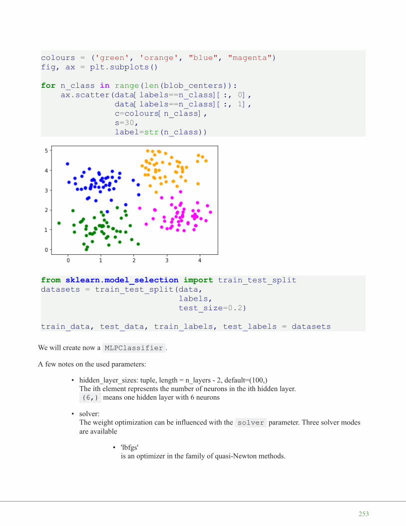
colours = ('green', 'orange', "blue", "magenta")fig, ax = plt.subplots()
for n_class in range(len(blob_centers)):ax.scatter(data[labels==n_class][:, 0],
data[labels==n_class][:, 1],c=colours[n_class],s=30,label=str(n_class))
from sklearn.model_selection import train_test_splitdatasets = train_test_split(data,
labels,test_size=0.2)
train_data, test_data, train_labels, test_labels = datasets
We will create now a MLPClassifier .
A few notes on the used parameters:
• hidden_layer_sizes: tuple, length = n_layers - 2, default=(100,)The ith element represents the number of neurons in the ith hidden layer.(6,) means one hidden layer with 6 neurons
• solver:The weight optimization can be influenced with the solver parameter. Three solver modesare available
▪ 'lbfgs'is an optimizer in the family of quasi-Newton methods.
253

▪ 'sgd'refers to stochastic gradient descent.
▪ 'adam' refers to a stochastic gradient-based optimizer proposed by Kingma,Diederik, and Jimmy Ba
Without understanding in the details of the solvers, you should know the following: 'adam'works pretty well - both training time and validation score - on relatively large datasets, i.e.thousands of training samples or more. For small datasets, however, 'lbfgs' can converge fasterand perform better.
• 'alpha'This parameter can be used to control possible 'overfitting' and 'underfitting'. We will cover it indetail further down in this chapter.
from sklearn.neural_network import MLPClassifier
clf = MLPClassifier(solver='lbfgs',alpha=1e-5,hidden_layer_sizes=(6,),random_state=1)
clf.fit(train_data, train_labels)
clf.score(train_data, train_labels)
from sklearn.metrics import accuracy_score
predictions_train = clf.predict(train_data)predictions_test = clf.predict(test_data)train_score = accuracy_score(predictions_train, train_labels)print("score on train data: ", train_score)test_score = accuracy_score(predictions_test, test_labels)print("score on train data: ", test_score)
predictions_train[:20]
Output: MLPClassifier(alpha=1e-05, hidden_layer_sizes=(6,), random_state=1,
solver='lbfgs')
Output: 1.0
score on train data: 1.0score on train data: 0.95
Output: array([2, 0, 1, 0, 2, 1, 3, 0, 3, 0, 2, 2, 1, 1, 0, 0, 1, 2,2, 3])
254

MULTI-LAYER PERCEPTRONfrom sklearn.neural_network import MLPClassifierX = [[0., 0.], [0., 1.], [1., 0.], [1., 1.]]y = [0, 0, 0, 1]clf = MLPClassifier(solver='lbfgs', alpha=1e-5,
hidden_layer_sizes=(5, 2), random_state=1)
print(clf.fit(X, y))
The following diagram depicts the neural network, that we have trained for our classifier clf. We have twoinput nodes X0 and X1, called the input layer, and one output neuron 'Out'. We have two hidden layers the first
one with the neurons H00 ... H04 and the second hidden layer consisting of H10 and H11. Each neuron of the
hidden layers and the output neuron possesses a corresponding Bias, i.e. B00 is the corresponding Bias to the
neuron H00, B01 is the corresponding Bias to the neuron H01 and so on.
Each neuron of the hidden layers receives the output from every neuron of the previous layers and transformsthese values with a weighted linear summation
n − 1
∑i = 0
wixi = w0x0 + w1x1 + . . . + wn − 1xn − 1
into an output value, where n is the number of neurons of the layer and wi corresponds to the ith component of
the weight vector. The output layer receives the values from the last hidden layer. It also performs a linearsummation, but a non-linear activation function
g( ⋅ ) : R → R
like the hyperbolic tan function will be applied to the summation result.
MLPClassifier(alpha=1e-05, hidden_layer_sizes=(5, 2), random_state=1,
solver='lbfgs')
255

The attribute coefs_ contains a list ofweight matrices for every layer. Theweight matrix at index i holds the weightsbetween the layer i and layer i + 1.
In [ ]:
print("weights between input and first hidden layer:")print(clf.coefs_[0])print("\nweights betweenfirst hidden and second hidden layer:")print(clf.coefs_[1])
The summation formula of the neuron H00 is defined by:
n − 1
∑i = 0
wixi = w0x0 + w1x1 + wB11∗ B11
which can be written as
n − 1
∑i = 0
wixi = w0x0 + w1x1 + wB11
because B11 = 1.
We can get the values for w0 and w1 from clf.coefs_ like this:
w0 = clf.coefs_[0][0][0] and w1 = clf.coefs_[0][1][0]
In [ ]:
print("w0 = ", clf.coefs_[0][0][0])print("w1 = ", clf.coefs_[0][1][0])
The weight vector of H00 can be accessed with
In [ ]:
clf.coefs_[0][:,0]
256

We can generalize the above to access a neuron Hij in the following way:
In [ ]:
for i in range(len(clf.coefs_)):number_neurons_in_layer = clf.coefs_[i].shape[1]for j in range(number_neurons_in_layer):
weights = clf.coefs_[i][:,j]print(i, j, weights, end=", ")print()
print()
intercepts_ is a list of bias vectors, where the vector at index i represents the bias values added to layer i+1.
In [ ]:
print("Bias values for first hidden layer:")print(clf.intercepts_[0])print("\nBias values for second hidden layer:")print(clf.intercepts_[1])
The main reason, why we train a classifier is to predict results for new samples. We can do this with thepredict method. The method returns a predicted class for a sample, in our case a "0" or a "1" :
In [ ]:
result = clf.predict([[0, 0], [0, 1],[1, 0], [0, 1],[1, 1], [2., 2.],[1.3, 1.3], [2, 4.8]])
Instead of just looking at the class results, we can also use the predict_proba method to get the probabilityestimates.
In [ ]:
prob_results = clf.predict_proba([[0, 0], [0, 1],[1, 0], [0, 1],[1, 1], [2., 2.],[1.3, 1.3], [2, 4.8]])
print(prob_results)
prob_results[i][0] gives us the probability for the class0, i.e. a "0" and results[i][1] the probabilty for a "1". i
corresponds to the ith sample.
COMPLETE IRIS DATASET EXAMPLE
257

from sklearn.datasets import load_iris
iris = load_iris()# splitting into train and test datasets
from sklearn.model_selection import train_test_splitdatasets = train_test_split(iris.data, iris.target,
test_size=0.2)
train_data, test_data, train_labels, test_labels = datasets# scaling the datafrom sklearn.preprocessing import StandardScalerscaler = StandardScaler()
# we fit the train datascaler.fit(train_data)
# scaling the train datatrain_data = scaler.transform(train_data)test_data = scaler.transform(test_data)
print(train_data[:3])
# Training the Modelfrom sklearn.neural_network import MLPClassifier# creating an classifier from the model:mlp = MLPClassifier(hidden_layer_sizes=(10, 5), max_iter=1000)
# let's fit the training data to our modelmlp.fit(train_data, train_labels)
from sklearn.metrics import accuracy_score
predictions_train = mlp.predict(train_data)print(accuracy_score(predictions_train, train_labels))predictions_test = mlp.predict(test_data)print(accuracy_score(predictions_test, test_labels))
[[ 1.91343191 -0.6013337 1.31398787 0.89583493][-0.93504278 1.48689909 -1.31208492 -1.08512683][ 0.4272712 -0.36930784 0.28639417 0.10345022]]
Output: MLPClassifier(hidden_layer_sizes=(10, 5), max_iter=1000)
258

from sklearn.metrics import confusion_matrix
confusion_matrix(predictions_train, train_labels)
confusion_matrix(predictions_test, test_labels)
from sklearn.metrics import classification_report
print(classification_report(predictions_test, test_labels))
MNIST DATASET
We have already used the MNIST dataset in the chapter Testing with MNIST of our tutorial. You will also findsome explanations about this dataset.
We want to apply the MLPClassifier on the MNIST data. We can load in the data with pickle:
import picklewith open("data/mnist/pickled_mnist.pkl", "br") as fh:
data = pickle.load(fh)
train_imgs = data[0]test_imgs = data[1]train_labels = data[2]
0.9750.9666666666666667
Output: array([[42, 0, 0],[ 0, 37, 1],[ 0, 2, 38]])
Output: array([[ 8, 0, 0],[ 0, 10, 0],[ 0, 1, 11]])
precision recall f1-score support
0 1.00 1.00 1.00 81 0.91 1.00 0.95 102 1.00 0.92 0.96 12
accuracy 0.97 30macro avg 0.97 0.97 0.97 30
weighted avg 0.97 0.97 0.97 30
259

test_labels = data[3]train_labels_one_hot = data[4]test_labels_one_hot = data[5]
image_size = 28 # width and lengthno_of_different_labels = 10 # i.e. 0, 1, 2, 3, ..., 9image_pixels = image_size * image_sizemlp = MLPClassifier(hidden_layer_sizes=(100, ),
max_iter=480, alpha=1e-4,solver='sgd', verbose=10,tol=1e-4, random_state=1,learning_rate_init=.1)
train_labels = train_labels.reshape(train_labels.shape[0],)print(train_imgs.shape, train_labels.shape)
mlp.fit(train_imgs, train_labels)print("Training set score: %f" % mlp.score(train_imgs, train_labels))print("Test set score: %f" % mlp.score(test_imgs, test_labels))
260

(60000, 784) (60000,)Iteration 1, loss = 0.29753549Iteration 2, loss = 0.12369769Iteration 3, loss = 0.08872688Iteration 4, loss = 0.07084598Iteration 5, loss = 0.05874947Iteration 6, loss = 0.04876359Iteration 7, loss = 0.04203350Iteration 8, loss = 0.03525624Iteration 9, loss = 0.02995642Iteration 10, loss = 0.02526208Iteration 11, loss = 0.02195436Iteration 12, loss = 0.01825246Iteration 13, loss = 0.01543440Iteration 14, loss = 0.01320164Iteration 15, loss = 0.01057486Iteration 16, loss = 0.00984482Iteration 17, loss = 0.00776886Iteration 18, loss = 0.00655891Iteration 19, loss = 0.00539189Iteration 20, loss = 0.00460981Iteration 21, loss = 0.00396910Iteration 22, loss = 0.00350800Iteration 23, loss = 0.00328115Iteration 24, loss = 0.00294118Iteration 25, loss = 0.00265852Iteration 26, loss = 0.00241809Iteration 27, loss = 0.00234944Iteration 28, loss = 0.00215147Iteration 29, loss = 0.00201855Iteration 30, loss = 0.00187808Iteration 31, loss = 0.00183098Iteration 32, loss = 0.00172363Iteration 33, loss = 0.00169482Iteration 34, loss = 0.00159811Iteration 35, loss = 0.00152427Iteration 36, loss = 0.00148731Iteration 37, loss = 0.00144202Iteration 38, loss = 0.00138101Iteration 39, loss = 0.00133767Iteration 40, loss = 0.00130437Iteration 41, loss = 0.00126314Iteration 42, loss = 0.00122969Iteration 43, loss = 0.00119848Training loss did not improve more than tol=0.000100 for 10 consecutive epochs. Stopping.
261

fig, axes = plt.subplots(4, 4)# use global min / max to ensure all weights are shown on the same scalevmin, vmax = mlp.coefs_[0].min(), mlp.coefs_[0].max()for coef, ax in zip(mlp.coefs_[0].T, axes.ravel()):
ax.matshow(coef.reshape(28, 28), cmap=plt.cm.gray, vmin=.5 * vmin,
vmax=.5 * vmax)ax.set_xticks(())ax.set_yticks(())
plt.show()
Training set score: 1.000000Test set score: 0.977900Help on method fit in module sklearn.neural_network._multilayer_perceptron:
fit(X, y) method of sklearn.neural_network._multilayer_perceptron.MLPClassifier instance
Fit the model to data matrix X and target(s) y.
Parameters----------X : ndarray or sparse matrix of shape (n_samples, n_features)
The input data.
y : ndarray, shape (n_samples,) or (n_samples, n_outputs)The target values (class labels in classification, real nu
mbers inregression).
Returns-------self : returns a trained MLP model.
262

THE PARAMETER ALPHA
A comparison of different values for regularization parameter ‘alpha’ on synthetic datasets. The plot showsthat different alphas yield different decision functions.
Alpha is a parameter for regularization term, aka penalty term, that combats overfitting by constraining thesize of the weights. Increasing alpha may fix high variance (a sign of overfitting) by encouraging smallerweights, resulting in a decision boundary plot that appears with lesser curvatures. Similarly, decreasing alphamay fix high bias (a sign of underfitting) by encouraging larger weights, potentially resulting in a morecomplicated decision boundary.
# Author: Issam H. Laradji# License: BSD 3 clause# code from: https://scikit-learn.org/stable/auto_examples/neural_networks/plot_mlp_alpha.html
import numpy as npfrom matplotlib import pyplot as pltfrom matplotlib.colors import ListedColormapfrom sklearn.model_selection import train_test_splitfrom sklearn.preprocessing import StandardScalerfrom sklearn.datasets import make_moons, make_circles, make_classificationfrom sklearn.neural_network import MLPClassifierfrom sklearn.pipeline import make_pipeline
h = .02 # step size in the mesh
alphas = np.logspace(-1, 1, 5)
classifiers = []
263

names = []for alpha in alphas:
classifiers.append(make_pipeline(StandardScaler(),MLPClassifier(
solver='lbfgs', alpha=alpha, random_state=1, max_iter=2000,
early_stopping=True, hidden_layer_sizes=[100, 100],)
))names.append(f"alpha {alpha:.2f}")
X, y = make_classification(n_features=2, n_redundant=0, n_informative=2,
random_state=0, n_clusters_per_class=1)rng = np.random.RandomState(2)X += 2 * rng.uniform(size=X.shape)linearly_separable = (X, y)
datasets = [make_moons(noise=0.3, random_state=0),make_circles(noise=0.2, factor=0.5, random_state=1),linearly_separable]
figure = plt.figure(figsize=(17, 9))i = 1# iterate over datasetsfor X, y in datasets:
# split into training and test partX_train, X_test, y_train, y_test = train_test_split(X, y, tes
t_size=.4)
x_min, x_max = X[:, 0].min() - .5, X[:, 0].max() + .5y_min, y_max = X[:, 1].min() - .5, X[:, 1].max() + .5xx, yy = np.meshgrid(np.arange(x_min, x_max, h),
np.arange(y_min, y_max, h))
# just plot the dataset firstcm = plt.cm.RdBucm_bright = ListedColormap(['#FF0000', '#0000FF'])ax = plt.subplot(len(datasets), len(classifiers) + 1, i)# Plot the training pointsax.scatter(X_train[:, 0], X_train[:, 1], c=y_train, cmap=cm_br
ight)# and testing pointsax.scatter(X_test[:, 0], X_test[:, 1], c=y_test, cmap=cm_brigh
264

t, alpha=0.6)ax.set_xlim(xx.min(), xx.max())ax.set_ylim(yy.min(), yy.max())ax.set_xticks(())ax.set_yticks(())i += 1
# iterate over classifiersfor name, clf in zip(names, classifiers):
ax = plt.subplot(len(datasets), len(classifiers) + 1, i)clf.fit(X_train, y_train)score = clf.score(X_test, y_test)
# Plot the decision boundary. For that, we will assign a color to each
# point in the mesh [x_min, x_max] x [y_min, y_max].if hasattr(clf, "decision_function"):
Z = clf.decision_function(np.c_[xx.ravel(), yy.ravel()])
else:Z = clf.predict_proba(np.c_[xx.ravel(), yy.rave
l()])[:, 1]
# Put the result into a color plotZ = Z.reshape(xx.shape)ax.contourf(xx, yy, Z, cmap=cm, alpha=.8)
# Plot also the training pointsax.scatter(X_train[:, 0], X_train[:, 1], c=y_train, cmap=c
m_bright,edgecolors='black', s=25)
# and testing pointsax.scatter(X_test[:, 0], X_test[:, 1], c=y_test, cmap=cm_b
right,alpha=0.6, edgecolors='black', s=25)
ax.set_xlim(xx.min(), xx.max())ax.set_ylim(yy.min(), yy.max())ax.set_xticks(())ax.set_yticks(())ax.set_title(name)ax.text(xx.max() - .3, yy.min() + .3, ('%.2f' % score).lst
rip('0'),size=15, horizontalalignment='right')
i += 1
265

figure.subplots_adjust(left=.02, right=.98)plt.show()
EXERCISES
EXERCISE 1
Classify the data in "strange_flowers.txt" with a k nearest neighbor classifier.
SOLUTIONS
SOLUTION TO EXERCISE 1
We use read_csv of the pandas module to read in the strange_flowers.txt file:
import pandas as pddataset = pd.read_csv("data/strange_flowers.txt",
header=None,names=["red", "green", "blue", "size", "labe
l"],sep=" ")
dataset
266

The first four columns contain the data and the last column contains the labels:
data = dataset.drop('label', axis=1)labels = dataset.labelX_train, X_test, y_train, y_test = train_test_split(data,
labels,random_stat
e=0,test_siz
e=0.2)
We have to scale the data now to reduce the biases between the data:
from sklearn.preprocessing import StandardScalerscaler = StandardScaler()
Output:
red green blue size label
0 238.0 104.0 8.0 3.65 1.0
1 235.0 114.0 9.0 4.00 1.0
2 252.0 93.0 9.0 3.71 1.0
3 242.0 116.0 9.0 3.67 1.0
4 251.0 117.0 15.0 3.49 1.0
... ... ... ... ... ...
790 0.0 248.0 98.0 3.03 4.0
791 0.0 253.0 106.0 2.85 4.0
792 0.0 250.0 91.0 3.39 4.0
793 0.0 248.0 99.0 3.10 4.0
794 0.0 244.0 109.0 2.96 4.0
795 rows × 5 columns
267

X_train = scaler.fit_transform(X_train) # transformX_test = scaler.transform(X_test) # transform
from sklearn.neural_network import MLPClassifier
mlp = MLPClassifier(hidden_layer_sizes=(100, ),max_iter=480,alpha=1e-4,solver='sgd',tol=1e-4,random_state=1,learning_rate_init=.1)
mlp.fit(X_train, y_train)print("Training set score: %f" % mlp.score(X_train, y_train))print("Test set score: %f" % mlp.score(X_test, y_test))Training set score: 0.971698Test set score: 0.981132
268

A N E U R A L N E T W O R K F O R T H E D I G I T SD A T A S E T
INTRODUCTION
The Python module sklear contains adataset with handwritten digits. It is justone of many datasets which sklearnprovides, as we show in our chapterRepresentation and Visualization of Data.In this chapter of our Machine Learningtutorial we will demonstrate how to createa neural network for the digits dataset torecognize these digits. This example isaccompanying the theoreticalintroductions of our previous chapters togive a practical view. You will see thathardly any Python code is needed toaccomplish the actual classification andrecognition task.
We will first load the digits data:
In [ ]:
from sklearn.datasets import load_digitsdigits = load_digits()
We can get an overview of what iscontained in the dataset with the keys method:
digits.keys()
The digits dataset contains 1797 images and each images contains 64 features, which correspond to the pixels:
Output: dict_keys(['data', 'target', 'frame', 'feature_names', 'target_names', 'images', 'DESCR'])
269

n_samples, n_features = digits.data.shapeprint((n_samples, n_features))
print(digits.data[0])
print(digits.target)
The data is also available at digits.images. This is the raw data of the images in the form of 8 lines and 8columns.
With "data" an image corresponds to a one-dimensional Numpy array with the length 64, and "images"representation contains 2-dimensional numpy arrays with the shape (8, 8)
print("Shape of an item: ", digits.data[0].shape)print("Data type of an item: ", type(digits.data[0]))print("Shape of an item: ", digits.images[0].shape)print("Data tpye of an item: ", type(digits.images[0]))
Let's visualize the data:
import matplotlib.pyplot as pltplt.imshow(digits.images[0], cmap='binary')plt.show()
(1797, 64)
[ 0. 0. 5. 13. 9. 1. 0. 0. 0. 0. 13. 15. 10. 15. 5. 0.0. 3.15. 2. 0. 11. 8. 0. 0. 4. 12. 0. 0. 8. 8. 0. 0. 5.
8. 0.0. 9. 8. 0. 0. 4. 11. 0. 1. 12. 7. 0. 0. 2. 14. 5. 1
0. 12.0. 0. 0. 0. 6. 13. 10. 0. 0. 0.]
[0 1 2 ... 8 9 8]
Shape of an item: (64,)Data type of an item: <class 'numpy.ndarray'>Shape of an item: (8, 8)Data tpye of an item: <class 'numpy.ndarray'>
270

Let's visualize some more digits combined with their labels:
import matplotlib.pyplot as plt# set up the figurefig = plt.figure(figsize=(6, 6)) # figure size in inchesfig.subplots_adjust(left=0, right=1, bottom=0, top=1, hspace=0.05, wspace=0.05)
# plot the digits: each image is 8x8 pixelsfor i in range(64):
ax = fig.add_subplot(8, 8, i + 1, xticks=[], yticks=[])ax.imshow(digits.images[i], cmap=plt.cm.binary, interpolatio
n='nearest')
# label the image with the target valueax.text(0, 7, str(digits.target[i]))
271

import matplotlib.pyplot as plt# set up the figurefig = plt.figure(figsize=(6, 6)) # figure size in inchesfig.subplots_adjust(left=0, right=1, bottom=0, top=1, hspace=0.05, wspace=0.05)
# plot the digits: each image is 8x8 pixelsfor i in range(144):
ax = fig.add_subplot(12, 12, i + 1, xticks=[], yticks=[])ax.imshow(digits.images[i], cmap=plt.cm.binary, interpolatio
n='nearest')
# label the image with the target value#ax.text(0, 7, str(digits.target[i]))
272

from sklearn.model_selection import train_test_split
res = train_test_split(digits.data, digits.target,train_size=0.8,test_size=0.2,random_state=1)
train_data, test_data, train_labels, test_labels = resfrom sklearn.neural_network import MLPClassifier
mlp = MLPClassifier(hidden_layer_sizes=(5,),activation='logistic',alpha=1e-4,solver='sgd',tol=1e-4,random_state=1,learning_rate_init=.3,verbose=True)
273

mlp.fit(train_data, train_labels)
274

Iteration 1, loss = 2.25145782Iteration 2, loss = 1.97730357Iteration 3, loss = 1.66620880Iteration 4, loss = 1.41353830Iteration 5, loss = 1.29575643Iteration 6, loss = 1.06663573Iteration 7, loss = 0.95558862Iteration 8, loss = 0.94767318Iteration 9, loss = 0.95242867Iteration 10, loss = 0.83577430Iteration 11, loss = 0.74541414Iteration 12, loss = 0.72011102Iteration 13, loss = 0.70790928Iteration 14, loss = 0.69425700Iteration 15, loss = 0.74458525Iteration 16, loss = 0.67779333Iteration 17, loss = 0.69691846Iteration 18, loss = 0.67844516Iteration 19, loss = 0.68164743Iteration 20, loss = 0.68435917Iteration 21, loss = 0.61988051Iteration 22, loss = 0.61362164Iteration 23, loss = 0.56615517Iteration 24, loss = 0.61323269Iteration 25, loss = 0.56979209Iteration 26, loss = 0.58189564Iteration 27, loss = 0.50692207Iteration 28, loss = 0.65956191Iteration 29, loss = 0.53736180Iteration 30, loss = 0.66437126Iteration 31, loss = 0.56201738Iteration 32, loss = 0.85347048Iteration 33, loss = 0.63673358Iteration 34, loss = 0.69769079Iteration 35, loss = 0.62714187Iteration 36, loss = 0.56914708Iteration 37, loss = 1.05660379Iteration 38, loss = 0.66966105Training loss did not improve more than tol=0.000100 for 10 consecutive epochs. Stopping.
275

predictions = mlp.predict(test_data)predictions[:25] , test_labels[:25]
from sklearn.metrics import accuracy_scoreaccuracy_score(test_labels, predictions)
for i in range(5, 30):mlp = MLPClassifier(hidden_layer_sizes=(i,),
activation='logistic',random_state=1,alpha=1e-4,solver='sgd',tol=1e-4,learning_rate_init=.3,verbose=False)
mlp.fit(train_data, train_labels)predictions = mlp.predict(test_data)acc_score = accuracy_score(test_labels, predictions)print(i, acc_score)
Output: MLPClassifier(activation='logistic', alpha=0.0001, batch_size='auto',
beta_1=0.9, beta_2=0.999, early_stopping=False, epsilon=1e-08,
hidden_layer_sizes=(5,), learning_rate='constant',learning_rate_init=0.3, max_iter=200, momentum=0.9,n_iter_no_change=10, nesterovs_momentum=True, powe
r_t=0.5,random_state=1, shuffle=True, solver='sgd', tol=0.000
1,validation_fraction=0.1, verbose=True, warm_start=Fals
e)
Output: (array([1, 5, 0, 7, 7, 0, 6, 1, 5, 4, 9, 2, 7, 8, 4, 1, 7,3, 7, 4, 7, 4,
8, 6, 0]),array([1, 5, 0, 7, 1, 0, 6, 1, 5, 4, 9, 2, 7, 8, 4, 6, 9,
3, 7, 4, 7, 1,8, 6, 0]))
Output: 0.725
276

In [ ]:
In [ ]:
In [ ]:
In [ ]:
from sklearn.model_selection import GridSearchCV
5 0.7256 0.372222222222222237 0.81666666666666678 0.86666666666666679 0.880555555555555510 0.92511 0.938888888888888912 0.938888888888888913 0.938888888888888914 0.952777777777777715 0.930555555555555616 0.9517 0.891666666666666718 0.8638888888888889/home/bernd/anaconda3/lib/python3.7/site-packages/sklearn/neural_network/multilayer_perceptron.py:562: ConvergenceWarning: Stochastic Optimizer: Maximum iterations (200) reached and the optimization hasn't converged yet.
% self.max_iter, ConvergenceWarning)19 0.955555555555555620 0.963888888888888921 0.972222222222222222 0.961111111111111123 0.944444444444444424 0.958333333333333425 0.930555555555555626 0.972222222222222227 0.969444444444444428 0.97529 0.9611111111111111
277

param_grid = [{
'activation' : ['identity', 'logistic', 'tanh', 'relu'],
'solver' : ['lbfgs', 'sgd', 'adam'],'hidden_layer_sizes': [(1,),(2,),(3,),(4,),(5,),(6,),(7,),(8,),(9,),(10,),(1
1,), (12,),(13,),(14,),(15,),(16,),(17,),(18,),(19,),(20,),(21,)]
}]
In [ ]:
clf = GridSearchCV(MLPClassifier(), param_grid, cv=3,scoring='accuracy')
clf.fit(train_data, train_labels)
print("Best parameters set found on development set:")print(clf.best_params_)
278

/home/bernd/anaconda3/lib/python3.7/site-packages/sklearn/neural_network/multilayer_perceptron.py:562: ConvergenceWarning: Stochastic Optimizer: Maximum iterations (200) reached and the optimization hasn't converged yet.
% self.max_iter, ConvergenceWarning)/home/bernd/anaconda3/lib/python3.7/site-packages/sklearn/neural_network/multilayer_perceptron.py:562: ConvergenceWarning: Stochastic Optimizer: Maximum iterations (200) reached and the optimization hasn't converged yet.
% self.max_iter, ConvergenceWarning)/home/bernd/anaconda3/lib/python3.7/site-packages/sklearn/neural_network/multilayer_perceptron.py:562: ConvergenceWarning: Stochastic Optimizer: Maximum iterations (200) reached and the optimization hasn't converged yet.
% self.max_iter, ConvergenceWarning)/home/bernd/anaconda3/lib/python3.7/site-packages/sklearn/neural_network/multilayer_perceptron.py:562: ConvergenceWarning: Stochastic Optimizer: Maximum iterations (200) reached and the optimization hasn't converged yet.
% self.max_iter, ConvergenceWarning)/home/bernd/anaconda3/lib/python3.7/site-packages/sklearn/neural_network/multilayer_perceptron.py:562: ConvergenceWarning: Stochastic Optimizer: Maximum iterations (200) reached and the optimization hasn't converged yet.
% self.max_iter, ConvergenceWarning)/home/bernd/anaconda3/lib/python3.7/site-packages/sklearn/neural_network/multilayer_perceptron.py:562: ConvergenceWarning: Stochastic Optimizer: Maximum iterations (200) reached and the optimization hasn't converged yet.
% self.max_iter, ConvergenceWarning)/home/bernd/anaconda3/lib/python3.7/site-packages/sklearn/neural_network/multilayer_perceptron.py:562: ConvergenceWarning: Stochastic Optimizer: Maximum iterations (200) reached and the optimization hasn't converged yet.
% self.max_iter, ConvergenceWarning)/home/bernd/anaconda3/lib/python3.7/site-packages/sklearn/neural_network/multilayer_perceptron.py:562: ConvergenceWarning: Stochastic Optimizer: Maximum iterations (200) reached and the optimization hasn't converged yet.
% self.max_iter, ConvergenceWarning)/home/bernd/anaconda3/lib/python3.7/site-packages/sklearn/neural_network/multilayer_perceptron.py:562: ConvergenceWarning: Stochastic Optimizer: Maximum iterations (200) reached and the optimization hasn't converged yet.
% self.max_iter, ConvergenceWarning)/home/bernd/anaconda3/lib/python3.7/site-packages/sklearn/neural_n
279

etwork/multilayer_perceptron.py:562: ConvergenceWarning: Stochastic Optimizer: Maximum iterations (200) reached and the optimization hasn't converged yet.
% self.max_iter, ConvergenceWarning)/home/bernd/anaconda3/lib/python3.7/site-packages/sklearn/neural_network/multilayer_perceptron.py:562: ConvergenceWarning: Stochastic Optimizer: Maximum iterations (200) reached and the optimization hasn't converged yet.
% self.max_iter, ConvergenceWarning)/home/bernd/anaconda3/lib/python3.7/site-packages/sklearn/neural_network/multilayer_perceptron.py:562: ConvergenceWarning: Stochastic Optimizer: Maximum iterations (200) reached and the optimization hasn't converged yet.
% self.max_iter, ConvergenceWarning)/home/bernd/anaconda3/lib/python3.7/site-packages/sklearn/neural_network/multilayer_perceptron.py:562: ConvergenceWarning: Stochastic Optimizer: Maximum iterations (200) reached and the optimization hasn't converged yet.
% self.max_iter, ConvergenceWarning)/home/bernd/anaconda3/lib/python3.7/site-packages/sklearn/neural_network/multilayer_perceptron.py:562: ConvergenceWarning: Stochastic Optimizer: Maximum iterations (200) reached and the optimization hasn't converged yet.
% self.max_iter, ConvergenceWarning)/home/bernd/anaconda3/lib/python3.7/site-packages/sklearn/neural_network/multilayer_perceptron.py:562: ConvergenceWarning: Stochastic Optimizer: Maximum iterations (200) reached and the optimization hasn't converged yet.
% self.max_iter, ConvergenceWarning)/home/bernd/anaconda3/lib/python3.7/site-packages/sklearn/neural_network/multilayer_perceptron.py:562: ConvergenceWarning: Stochastic Optimizer: Maximum iterations (200) reached and the optimization hasn't converged yet.
% self.max_iter, ConvergenceWarning)/home/bernd/anaconda3/lib/python3.7/site-packages/sklearn/neural_network/multilayer_perceptron.py:562: ConvergenceWarning: Stochastic Optimizer: Maximum iterations (200) reached and the optimization hasn't converged yet.
% self.max_iter, ConvergenceWarning)/home/bernd/anaconda3/lib/python3.7/site-packages/sklearn/neural_network/multilayer_perceptron.py:562: ConvergenceWarning: Stochastic Optimizer: Maximum iterations (200) reached and the optimization hasn't converged yet.
% self.max_iter, ConvergenceWarning)/home/bernd/anaconda3/lib/python3.7/site-packages/sklearn/neural_network/multilayer_perceptron.py:562: ConvergenceWarning: Stochasti
280

c Optimizer: Maximum iterations (200) reached and the optimization hasn't converged yet.
% self.max_iter, ConvergenceWarning)/home/bernd/anaconda3/lib/python3.7/site-packages/sklearn/neural_network/multilayer_perceptron.py:562: ConvergenceWarning: Stochastic Optimizer: Maximum iterations (200) reached and the optimization hasn't converged yet.
% self.max_iter, ConvergenceWarning)/home/bernd/anaconda3/lib/python3.7/site-packages/sklearn/neural_network/multilayer_perceptron.py:562: ConvergenceWarning: Stochastic Optimizer: Maximum iterations (200) reached and the optimization hasn't converged yet.
% self.max_iter, ConvergenceWarning)/home/bernd/anaconda3/lib/python3.7/site-packages/sklearn/neural_network/multilayer_perceptron.py:562: ConvergenceWarning: Stochastic Optimizer: Maximum iterations (200) reached and the optimization hasn't converged yet.
% self.max_iter, ConvergenceWarning)/home/bernd/anaconda3/lib/python3.7/site-packages/sklearn/neural_network/multilayer_perceptron.py:562: ConvergenceWarning: Stochastic Optimizer: Maximum iterations (200) reached and the optimization hasn't converged yet.
% self.max_iter, ConvergenceWarning)/home/bernd/anaconda3/lib/python3.7/site-packages/sklearn/neural_network/multilayer_perceptron.py:562: ConvergenceWarning: Stochastic Optimizer: Maximum iterations (200) reached and the optimization hasn't converged yet.
% self.max_iter, ConvergenceWarning)/home/bernd/anaconda3/lib/python3.7/site-packages/sklearn/neural_network/multilayer_perceptron.py:562: ConvergenceWarning: Stochastic Optimizer: Maximum iterations (200) reached and the optimization hasn't converged yet.
% self.max_iter, ConvergenceWarning)/home/bernd/anaconda3/lib/python3.7/site-packages/sklearn/neural_network/multilayer_perceptron.py:562: ConvergenceWarning: Stochastic Optimizer: Maximum iterations (200) reached and the optimization hasn't converged yet.
% self.max_iter, ConvergenceWarning)/home/bernd/anaconda3/lib/python3.7/site-packages/sklearn/neural_network/multilayer_perceptron.py:562: ConvergenceWarning: Stochastic Optimizer: Maximum iterations (200) reached and the optimization hasn't converged yet.
% self.max_iter, ConvergenceWarning)/home/bernd/anaconda3/lib/python3.7/site-packages/sklearn/neural_network/multilayer_perceptron.py:562: ConvergenceWarning: Stochastic Optimizer: Maximum iterations (200) reached and the optimizatio
281

n hasn't converged yet.% self.max_iter, ConvergenceWarning)
/home/bernd/anaconda3/lib/python3.7/site-packages/sklearn/neural_network/multilayer_perceptron.py:562: ConvergenceWarning: Stochastic Optimizer: Maximum iterations (200) reached and the optimization hasn't converged yet.
% self.max_iter, ConvergenceWarning)/home/bernd/anaconda3/lib/python3.7/site-packages/sklearn/neural_network/multilayer_perceptron.py:562: ConvergenceWarning: Stochastic Optimizer: Maximum iterations (200) reached and the optimization hasn't converged yet.
% self.max_iter, ConvergenceWarning)/home/bernd/anaconda3/lib/python3.7/site-packages/sklearn/neural_network/multilayer_perceptron.py:562: ConvergenceWarning: Stochastic Optimizer: Maximum iterations (200) reached and the optimization hasn't converged yet.
% self.max_iter, ConvergenceWarning)/home/bernd/anaconda3/lib/python3.7/site-packages/sklearn/neural_network/multilayer_perceptron.py:562: ConvergenceWarning: Stochastic Optimizer: Maximum iterations (200) reached and the optimization hasn't converged yet.
% self.max_iter, ConvergenceWarning)/home/bernd/anaconda3/lib/python3.7/site-packages/sklearn/neural_network/multilayer_perceptron.py:562: ConvergenceWarning: Stochastic Optimizer: Maximum iterations (200) reached and the optimization hasn't converged yet.
% self.max_iter, ConvergenceWarning)/home/bernd/anaconda3/lib/python3.7/site-packages/sklearn/neural_network/multilayer_perceptron.py:562: ConvergenceWarning: Stochastic Optimizer: Maximum iterations (200) reached and the optimization hasn't converged yet.
% self.max_iter, ConvergenceWarning)/home/bernd/anaconda3/lib/python3.7/site-packages/sklearn/neural_network/multilayer_perceptron.py:562: ConvergenceWarning: Stochastic Optimizer: Maximum iterations (200) reached and the optimization hasn't converged yet.
% self.max_iter, ConvergenceWarning)/home/bernd/anaconda3/lib/python3.7/site-packages/sklearn/neural_network/multilayer_perceptron.py:562: ConvergenceWarning: Stochastic Optimizer: Maximum iterations (200) reached and the optimization hasn't converged yet.
% self.max_iter, ConvergenceWarning)/home/bernd/anaconda3/lib/python3.7/site-packages/sklearn/neural_network/multilayer_perceptron.py:562: ConvergenceWarning: Stochastic Optimizer: Maximum iterations (200) reached and the optimization hasn't converged yet.
282

% self.max_iter, ConvergenceWarning)/home/bernd/anaconda3/lib/python3.7/site-packages/sklearn/neural_network/multilayer_perceptron.py:562: ConvergenceWarning: Stochastic Optimizer: Maximum iterations (200) reached and the optimization hasn't converged yet.
% self.max_iter, ConvergenceWarning)/home/bernd/anaconda3/lib/python3.7/site-packages/sklearn/neural_network/multilayer_perceptron.py:562: ConvergenceWarning: Stochastic Optimizer: Maximum iterations (200) reached and the optimization hasn't converged yet.
% self.max_iter, ConvergenceWarning)/home/bernd/anaconda3/lib/python3.7/site-packages/sklearn/neural_network/multilayer_perceptron.py:562: ConvergenceWarning: Stochastic Optimizer: Maximum iterations (200) reached and the optimization hasn't converged yet.
% self.max_iter, ConvergenceWarning)/home/bernd/anaconda3/lib/python3.7/site-packages/sklearn/neural_network/multilayer_perceptron.py:562: ConvergenceWarning: Stochastic Optimizer: Maximum iterations (200) reached and the optimization hasn't converged yet.
% self.max_iter, ConvergenceWarning)/home/bernd/anaconda3/lib/python3.7/site-packages/sklearn/neural_network/multilayer_perceptron.py:562: ConvergenceWarning: Stochastic Optimizer: Maximum iterations (200) reached and the optimization hasn't converged yet.
% self.max_iter, ConvergenceWarning)/home/bernd/anaconda3/lib/python3.7/site-packages/sklearn/neural_network/multilayer_perceptron.py:562: ConvergenceWarning: Stochastic Optimizer: Maximum iterations (200) reached and the optimization hasn't converged yet.
% self.max_iter, ConvergenceWarning)/home/bernd/anaconda3/lib/python3.7/site-packages/sklearn/neural_network/multilayer_perceptron.py:562: ConvergenceWarning: Stochastic Optimizer: Maximum iterations (200) reached and the optimization hasn't converged yet.
% self.max_iter, ConvergenceWarning)/home/bernd/anaconda3/lib/python3.7/site-packages/sklearn/neural_network/multilayer_perceptron.py:562: ConvergenceWarning: Stochastic Optimizer: Maximum iterations (200) reached and the optimization hasn't converged yet.
% self.max_iter, ConvergenceWarning)/home/bernd/anaconda3/lib/python3.7/site-packages/sklearn/neural_network/multilayer_perceptron.py:562: ConvergenceWarning: Stochastic Optimizer: Maximum iterations (200) reached and the optimization hasn't converged yet.
% self.max_iter, ConvergenceWarning)
283

/home/bernd/anaconda3/lib/python3.7/site-packages/sklearn/neural_network/multilayer_perceptron.py:562: ConvergenceWarning: Stochastic Optimizer: Maximum iterations (200) reached and the optimization hasn't converged yet.
% self.max_iter, ConvergenceWarning)/home/bernd/anaconda3/lib/python3.7/site-packages/sklearn/neural_network/multilayer_perceptron.py:562: ConvergenceWarning: Stochastic Optimizer: Maximum iterations (200) reached and the optimization hasn't converged yet.
% self.max_iter, ConvergenceWarning)/home/bernd/anaconda3/lib/python3.7/site-packages/sklearn/neural_network/multilayer_perceptron.py:562: ConvergenceWarning: Stochastic Optimizer: Maximum iterations (200) reached and the optimization hasn't converged yet.
% self.max_iter, ConvergenceWarning)/home/bernd/anaconda3/lib/python3.7/site-packages/sklearn/neural_network/multilayer_perceptron.py:562: ConvergenceWarning: Stochastic Optimizer: Maximum iterations (200) reached and the optimization hasn't converged yet.
% self.max_iter, ConvergenceWarning)/home/bernd/anaconda3/lib/python3.7/site-packages/sklearn/neural_network/multilayer_perceptron.py:562: ConvergenceWarning: Stochastic Optimizer: Maximum iterations (200) reached and the optimization hasn't converged yet.
% self.max_iter, ConvergenceWarning)/home/bernd/anaconda3/lib/python3.7/site-packages/sklearn/neural_network/multilayer_perceptron.py:562: ConvergenceWarning: Stochastic Optimizer: Maximum iterations (200) reached and the optimization hasn't converged yet.
% self.max_iter, ConvergenceWarning)/home/bernd/anaconda3/lib/python3.7/site-packages/sklearn/neural_network/multilayer_perceptron.py:562: ConvergenceWarning: Stochastic Optimizer: Maximum iterations (200) reached and the optimization hasn't converged yet.
% self.max_iter, ConvergenceWarning)/home/bernd/anaconda3/lib/python3.7/site-packages/sklearn/neural_network/multilayer_perceptron.py:562: ConvergenceWarning: Stochastic Optimizer: Maximum iterations (200) reached and the optimization hasn't converged yet.
% self.max_iter, ConvergenceWarning)/home/bernd/anaconda3/lib/python3.7/site-packages/sklearn/neural_network/multilayer_perceptron.py:562: ConvergenceWarning: Stochastic Optimizer: Maximum iterations (200) reached and the optimization hasn't converged yet.
% self.max_iter, ConvergenceWarning)/home/bernd/anaconda3/lib/python3.7/site-packages/sklearn/neural_n
284

etwork/multilayer_perceptron.py:562: ConvergenceWarning: Stochastic Optimizer: Maximum iterations (200) reached and the optimization hasn't converged yet.
% self.max_iter, ConvergenceWarning)/home/bernd/anaconda3/lib/python3.7/site-packages/sklearn/neural_network/multilayer_perceptron.py:562: ConvergenceWarning: Stochastic Optimizer: Maximum iterations (200) reached and the optimization hasn't converged yet.
% self.max_iter, ConvergenceWarning)/home/bernd/anaconda3/lib/python3.7/site-packages/sklearn/neural_network/multilayer_perceptron.py:562: ConvergenceWarning: Stochastic Optimizer: Maximum iterations (200) reached and the optimization hasn't converged yet.
% self.max_iter, ConvergenceWarning)/home/bernd/anaconda3/lib/python3.7/site-packages/sklearn/neural_network/multilayer_perceptron.py:562: ConvergenceWarning: Stochastic Optimizer: Maximum iterations (200) reached and the optimization hasn't converged yet.
% self.max_iter, ConvergenceWarning)/home/bernd/anaconda3/lib/python3.7/site-packages/sklearn/neural_network/multilayer_perceptron.py:562: ConvergenceWarning: Stochastic Optimizer: Maximum iterations (200) reached and the optimization hasn't converged yet.
% self.max_iter, ConvergenceWarning)/home/bernd/anaconda3/lib/python3.7/site-packages/sklearn/neural_network/multilayer_perceptron.py:562: ConvergenceWarning: Stochastic Optimizer: Maximum iterations (200) reached and the optimization hasn't converged yet.
% self.max_iter, ConvergenceWarning)/home/bernd/anaconda3/lib/python3.7/site-packages/sklearn/neural_network/multilayer_perceptron.py:562: ConvergenceWarning: Stochastic Optimizer: Maximum iterations (200) reached and the optimization hasn't converged yet.
% self.max_iter, ConvergenceWarning)/home/bernd/anaconda3/lib/python3.7/site-packages/sklearn/neural_network/multilayer_perceptron.py:562: ConvergenceWarning: Stochastic Optimizer: Maximum iterations (200) reached and the optimization hasn't converged yet.
% self.max_iter, ConvergenceWarning)/home/bernd/anaconda3/lib/python3.7/site-packages/sklearn/neural_network/multilayer_perceptron.py:562: ConvergenceWarning: Stochastic Optimizer: Maximum iterations (200) reached and the optimization hasn't converged yet.
% self.max_iter, ConvergenceWarning)/home/bernd/anaconda3/lib/python3.7/site-packages/sklearn/neural_network/multilayer_perceptron.py:562: ConvergenceWarning: Stochasti
285

c Optimizer: Maximum iterations (200) reached and the optimization hasn't converged yet.
% self.max_iter, ConvergenceWarning)/home/bernd/anaconda3/lib/python3.7/site-packages/sklearn/neural_network/multilayer_perceptron.py:562: ConvergenceWarning: Stochastic Optimizer: Maximum iterations (200) reached and the optimization hasn't converged yet.
% self.max_iter, ConvergenceWarning)/home/bernd/anaconda3/lib/python3.7/site-packages/sklearn/neural_network/multilayer_perceptron.py:562: ConvergenceWarning: Stochastic Optimizer: Maximum iterations (200) reached and the optimization hasn't converged yet.
% self.max_iter, ConvergenceWarning)/home/bernd/anaconda3/lib/python3.7/site-packages/sklearn/neural_network/multilayer_perceptron.py:562: ConvergenceWarning: Stochastic Optimizer: Maximum iterations (200) reached and the optimization hasn't converged yet.
% self.max_iter, ConvergenceWarning)/home/bernd/anaconda3/lib/python3.7/site-packages/sklearn/neural_network/multilayer_perceptron.py:562: ConvergenceWarning: Stochastic Optimizer: Maximum iterations (200) reached and the optimization hasn't converged yet.
% self.max_iter, ConvergenceWarning)/home/bernd/anaconda3/lib/python3.7/site-packages/sklearn/neural_network/multilayer_perceptron.py:562: ConvergenceWarning: Stochastic Optimizer: Maximum iterations (200) reached and the optimization hasn't converged yet.
% self.max_iter, ConvergenceWarning)/home/bernd/anaconda3/lib/python3.7/site-packages/sklearn/neural_network/multilayer_perceptron.py:562: ConvergenceWarning: Stochastic Optimizer: Maximum iterations (200) reached and the optimization hasn't converged yet.
% self.max_iter, ConvergenceWarning)/home/bernd/anaconda3/lib/python3.7/site-packages/sklearn/neural_network/multilayer_perceptron.py:562: ConvergenceWarning: Stochastic Optimizer: Maximum iterations (200) reached and the optimization hasn't converged yet.
% self.max_iter, ConvergenceWarning)/home/bernd/anaconda3/lib/python3.7/site-packages/sklearn/neural_network/multilayer_perceptron.py:562: ConvergenceWarning: Stochastic Optimizer: Maximum iterations (200) reached and the optimization hasn't converged yet.
% self.max_iter, ConvergenceWarning)/home/bernd/anaconda3/lib/python3.7/site-packages/sklearn/neural_network/multilayer_perceptron.py:562: ConvergenceWarning: Stochastic Optimizer: Maximum iterations (200) reached and the optimizatio
286

n hasn't converged yet.% self.max_iter, ConvergenceWarning)
/home/bernd/anaconda3/lib/python3.7/site-packages/sklearn/neural_network/multilayer_perceptron.py:562: ConvergenceWarning: Stochastic Optimizer: Maximum iterations (200) reached and the optimization hasn't converged yet.
% self.max_iter, ConvergenceWarning)/home/bernd/anaconda3/lib/python3.7/site-packages/sklearn/neural_network/multilayer_perceptron.py:562: ConvergenceWarning: Stochastic Optimizer: Maximum iterations (200) reached and the optimization hasn't converged yet.
% self.max_iter, ConvergenceWarning)/home/bernd/anaconda3/lib/python3.7/site-packages/sklearn/neural_network/multilayer_perceptron.py:562: ConvergenceWarning: Stochastic Optimizer: Maximum iterations (200) reached and the optimization hasn't converged yet.
% self.max_iter, ConvergenceWarning)/home/bernd/anaconda3/lib/python3.7/site-packages/sklearn/neural_network/multilayer_perceptron.py:562: ConvergenceWarning: Stochastic Optimizer: Maximum iterations (200) reached and the optimization hasn't converged yet.
% self.max_iter, ConvergenceWarning)/home/bernd/anaconda3/lib/python3.7/site-packages/sklearn/neural_network/multilayer_perceptron.py:562: ConvergenceWarning: Stochastic Optimizer: Maximum iterations (200) reached and the optimization hasn't converged yet.
% self.max_iter, ConvergenceWarning)/home/bernd/anaconda3/lib/python3.7/site-packages/sklearn/neural_network/multilayer_perceptron.py:562: ConvergenceWarning: Stochastic Optimizer: Maximum iterations (200) reached and the optimization hasn't converged yet.
% self.max_iter, ConvergenceWarning)/home/bernd/anaconda3/lib/python3.7/site-packages/sklearn/neural_network/multilayer_perceptron.py:562: ConvergenceWarning: Stochastic Optimizer: Maximum iterations (200) reached and the optimization hasn't converged yet.
% self.max_iter, ConvergenceWarning)/home/bernd/anaconda3/lib/python3.7/site-packages/sklearn/neural_network/multilayer_perceptron.py:562: ConvergenceWarning: Stochastic Optimizer: Maximum iterations (200) reached and the optimization hasn't converged yet.
% self.max_iter, ConvergenceWarning)/home/bernd/anaconda3/lib/python3.7/site-packages/sklearn/neural_network/multilayer_perceptron.py:562: ConvergenceWarning: Stochastic Optimizer: Maximum iterations (200) reached and the optimization hasn't converged yet.
287
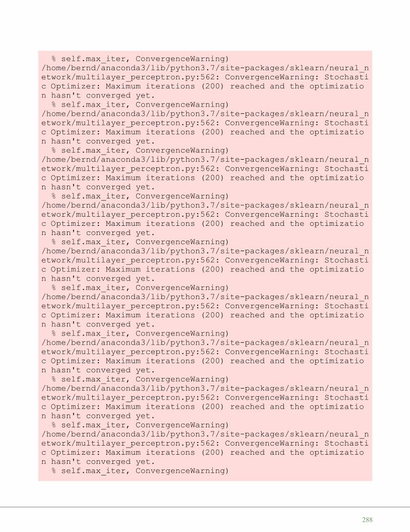
% self.max_iter, ConvergenceWarning)/home/bernd/anaconda3/lib/python3.7/site-packages/sklearn/neural_network/multilayer_perceptron.py:562: ConvergenceWarning: Stochastic Optimizer: Maximum iterations (200) reached and the optimization hasn't converged yet.
% self.max_iter, ConvergenceWarning)/home/bernd/anaconda3/lib/python3.7/site-packages/sklearn/neural_network/multilayer_perceptron.py:562: ConvergenceWarning: Stochastic Optimizer: Maximum iterations (200) reached and the optimization hasn't converged yet.
% self.max_iter, ConvergenceWarning)/home/bernd/anaconda3/lib/python3.7/site-packages/sklearn/neural_network/multilayer_perceptron.py:562: ConvergenceWarning: Stochastic Optimizer: Maximum iterations (200) reached and the optimization hasn't converged yet.
% self.max_iter, ConvergenceWarning)/home/bernd/anaconda3/lib/python3.7/site-packages/sklearn/neural_network/multilayer_perceptron.py:562: ConvergenceWarning: Stochastic Optimizer: Maximum iterations (200) reached and the optimization hasn't converged yet.
% self.max_iter, ConvergenceWarning)/home/bernd/anaconda3/lib/python3.7/site-packages/sklearn/neural_network/multilayer_perceptron.py:562: ConvergenceWarning: Stochastic Optimizer: Maximum iterations (200) reached and the optimization hasn't converged yet.
% self.max_iter, ConvergenceWarning)/home/bernd/anaconda3/lib/python3.7/site-packages/sklearn/neural_network/multilayer_perceptron.py:562: ConvergenceWarning: Stochastic Optimizer: Maximum iterations (200) reached and the optimization hasn't converged yet.
% self.max_iter, ConvergenceWarning)/home/bernd/anaconda3/lib/python3.7/site-packages/sklearn/neural_network/multilayer_perceptron.py:562: ConvergenceWarning: Stochastic Optimizer: Maximum iterations (200) reached and the optimization hasn't converged yet.
% self.max_iter, ConvergenceWarning)/home/bernd/anaconda3/lib/python3.7/site-packages/sklearn/neural_network/multilayer_perceptron.py:562: ConvergenceWarning: Stochastic Optimizer: Maximum iterations (200) reached and the optimization hasn't converged yet.
% self.max_iter, ConvergenceWarning)/home/bernd/anaconda3/lib/python3.7/site-packages/sklearn/neural_network/multilayer_perceptron.py:562: ConvergenceWarning: Stochastic Optimizer: Maximum iterations (200) reached and the optimization hasn't converged yet.
% self.max_iter, ConvergenceWarning)
288

/home/bernd/anaconda3/lib/python3.7/site-packages/sklearn/neural_network/multilayer_perceptron.py:562: ConvergenceWarning: Stochastic Optimizer: Maximum iterations (200) reached and the optimization hasn't converged yet.
% self.max_iter, ConvergenceWarning)/home/bernd/anaconda3/lib/python3.7/site-packages/sklearn/neural_network/multilayer_perceptron.py:562: ConvergenceWarning: Stochastic Optimizer: Maximum iterations (200) reached and the optimization hasn't converged yet.
% self.max_iter, ConvergenceWarning)/home/bernd/anaconda3/lib/python3.7/site-packages/sklearn/neural_network/multilayer_perceptron.py:562: ConvergenceWarning: Stochastic Optimizer: Maximum iterations (200) reached and the optimization hasn't converged yet.
% self.max_iter, ConvergenceWarning)/home/bernd/anaconda3/lib/python3.7/site-packages/sklearn/neural_network/multilayer_perceptron.py:562: ConvergenceWarning: Stochastic Optimizer: Maximum iterations (200) reached and the optimization hasn't converged yet.
% self.max_iter, ConvergenceWarning)/home/bernd/anaconda3/lib/python3.7/site-packages/sklearn/neural_network/multilayer_perceptron.py:562: ConvergenceWarning: Stochastic Optimizer: Maximum iterations (200) reached and the optimization hasn't converged yet.
% self.max_iter, ConvergenceWarning)/home/bernd/anaconda3/lib/python3.7/site-packages/sklearn/neural_network/multilayer_perceptron.py:562: ConvergenceWarning: Stochastic Optimizer: Maximum iterations (200) reached and the optimization hasn't converged yet.
% self.max_iter, ConvergenceWarning)/home/bernd/anaconda3/lib/python3.7/site-packages/sklearn/neural_network/multilayer_perceptron.py:562: ConvergenceWarning: Stochastic Optimizer: Maximum iterations (200) reached and the optimization hasn't converged yet.
% self.max_iter, ConvergenceWarning)/home/bernd/anaconda3/lib/python3.7/site-packages/sklearn/neural_network/multilayer_perceptron.py:562: ConvergenceWarning: Stochastic Optimizer: Maximum iterations (200) reached and the optimization hasn't converged yet.
% self.max_iter, ConvergenceWarning)/home/bernd/anaconda3/lib/python3.7/site-packages/sklearn/neural_network/multilayer_perceptron.py:562: ConvergenceWarning: Stochastic Optimizer: Maximum iterations (200) reached and the optimization hasn't converged yet.
% self.max_iter, ConvergenceWarning)/home/bernd/anaconda3/lib/python3.7/site-packages/sklearn/neural_n
289

etwork/multilayer_perceptron.py:562: ConvergenceWarning: Stochastic Optimizer: Maximum iterations (200) reached and the optimization hasn't converged yet.
% self.max_iter, ConvergenceWarning)/home/bernd/anaconda3/lib/python3.7/site-packages/sklearn/neural_network/multilayer_perceptron.py:562: ConvergenceWarning: Stochastic Optimizer: Maximum iterations (200) reached and the optimization hasn't converged yet.
% self.max_iter, ConvergenceWarning)/home/bernd/anaconda3/lib/python3.7/site-packages/sklearn/neural_network/multilayer_perceptron.py:562: ConvergenceWarning: Stochastic Optimizer: Maximum iterations (200) reached and the optimization hasn't converged yet.
% self.max_iter, ConvergenceWarning)/home/bernd/anaconda3/lib/python3.7/site-packages/sklearn/neural_network/multilayer_perceptron.py:562: ConvergenceWarning: Stochastic Optimizer: Maximum iterations (200) reached and the optimization hasn't converged yet.
% self.max_iter, ConvergenceWarning)/home/bernd/anaconda3/lib/python3.7/site-packages/sklearn/neural_network/multilayer_perceptron.py:562: ConvergenceWarning: Stochastic Optimizer: Maximum iterations (200) reached and the optimization hasn't converged yet.
% self.max_iter, ConvergenceWarning)/home/bernd/anaconda3/lib/python3.7/site-packages/sklearn/neural_network/multilayer_perceptron.py:562: ConvergenceWarning: Stochastic Optimizer: Maximum iterations (200) reached and the optimization hasn't converged yet.
% self.max_iter, ConvergenceWarning)/home/bernd/anaconda3/lib/python3.7/site-packages/sklearn/neural_network/multilayer_perceptron.py:562: ConvergenceWarning: Stochastic Optimizer: Maximum iterations (200) reached and the optimization hasn't converged yet.
% self.max_iter, ConvergenceWarning)/home/bernd/anaconda3/lib/python3.7/site-packages/sklearn/neural_network/multilayer_perceptron.py:562: ConvergenceWarning: Stochastic Optimizer: Maximum iterations (200) reached and the optimization hasn't converged yet.
% self.max_iter, ConvergenceWarning)/home/bernd/anaconda3/lib/python3.7/site-packages/sklearn/neural_network/multilayer_perceptron.py:562: ConvergenceWarning: Stochastic Optimizer: Maximum iterations (200) reached and the optimization hasn't converged yet.
% self.max_iter, ConvergenceWarning)/home/bernd/anaconda3/lib/python3.7/site-packages/sklearn/neural_network/multilayer_perceptron.py:562: ConvergenceWarning: Stochasti
290

c Optimizer: Maximum iterations (200) reached and the optimization hasn't converged yet.
% self.max_iter, ConvergenceWarning)/home/bernd/anaconda3/lib/python3.7/site-packages/sklearn/neural_network/multilayer_perceptron.py:562: ConvergenceWarning: Stochastic Optimizer: Maximum iterations (200) reached and the optimization hasn't converged yet.
% self.max_iter, ConvergenceWarning)/home/bernd/anaconda3/lib/python3.7/site-packages/sklearn/neural_network/multilayer_perceptron.py:562: ConvergenceWarning: Stochastic Optimizer: Maximum iterations (200) reached and the optimization hasn't converged yet.
% self.max_iter, ConvergenceWarning)/home/bernd/anaconda3/lib/python3.7/site-packages/sklearn/neural_network/multilayer_perceptron.py:562: ConvergenceWarning: Stochastic Optimizer: Maximum iterations (200) reached and the optimization hasn't converged yet.
% self.max_iter, ConvergenceWarning)/home/bernd/anaconda3/lib/python3.7/site-packages/sklearn/neural_network/multilayer_perceptron.py:562: ConvergenceWarning: Stochastic Optimizer: Maximum iterations (200) reached and the optimization hasn't converged yet.
% self.max_iter, ConvergenceWarning)/home/bernd/anaconda3/lib/python3.7/site-packages/sklearn/neural_network/multilayer_perceptron.py:562: ConvergenceWarning: Stochastic Optimizer: Maximum iterations (200) reached and the optimization hasn't converged yet.
% self.max_iter, ConvergenceWarning)/home/bernd/anaconda3/lib/python3.7/site-packages/sklearn/neural_network/multilayer_perceptron.py:562: ConvergenceWarning: Stochastic Optimizer: Maximum iterations (200) reached and the optimization hasn't converged yet.
% self.max_iter, ConvergenceWarning)/home/bernd/anaconda3/lib/python3.7/site-packages/sklearn/neural_network/multilayer_perceptron.py:562: ConvergenceWarning: Stochastic Optimizer: Maximum iterations (200) reached and the optimization hasn't converged yet.
% self.max_iter, ConvergenceWarning)/home/bernd/anaconda3/lib/python3.7/site-packages/sklearn/neural_network/multilayer_perceptron.py:562: ConvergenceWarning: Stochastic Optimizer: Maximum iterations (200) reached and the optimization hasn't converged yet.
% self.max_iter, ConvergenceWarning)/home/bernd/anaconda3/lib/python3.7/site-packages/sklearn/neural_network/multilayer_perceptron.py:562: ConvergenceWarning: Stochastic Optimizer: Maximum iterations (200) reached and the optimizatio
291

n hasn't converged yet.% self.max_iter, ConvergenceWarning)
/home/bernd/anaconda3/lib/python3.7/site-packages/sklearn/neural_network/multilayer_perceptron.py:562: ConvergenceWarning: Stochastic Optimizer: Maximum iterations (200) reached and the optimization hasn't converged yet.
% self.max_iter, ConvergenceWarning)/home/bernd/anaconda3/lib/python3.7/site-packages/sklearn/neural_network/multilayer_perceptron.py:562: ConvergenceWarning: Stochastic Optimizer: Maximum iterations (200) reached and the optimization hasn't converged yet.
% self.max_iter, ConvergenceWarning)/home/bernd/anaconda3/lib/python3.7/site-packages/sklearn/neural_network/multilayer_perceptron.py:562: ConvergenceWarning: Stochastic Optimizer: Maximum iterations (200) reached and the optimization hasn't converged yet.
% self.max_iter, ConvergenceWarning)/home/bernd/anaconda3/lib/python3.7/site-packages/sklearn/neural_network/multilayer_perceptron.py:562: ConvergenceWarning: Stochastic Optimizer: Maximum iterations (200) reached and the optimization hasn't converged yet.
% self.max_iter, ConvergenceWarning)/home/bernd/anaconda3/lib/python3.7/site-packages/sklearn/neural_network/multilayer_perceptron.py:562: ConvergenceWarning: Stochastic Optimizer: Maximum iterations (200) reached and the optimization hasn't converged yet.
% self.max_iter, ConvergenceWarning)/home/bernd/anaconda3/lib/python3.7/site-packages/sklearn/neural_network/multilayer_perceptron.py:562: ConvergenceWarning: Stochastic Optimizer: Maximum iterations (200) reached and the optimization hasn't converged yet.
% self.max_iter, ConvergenceWarning)/home/bernd/anaconda3/lib/python3.7/site-packages/sklearn/neural_network/multilayer_perceptron.py:562: ConvergenceWarning: Stochastic Optimizer: Maximum iterations (200) reached and the optimization hasn't converged yet.
% self.max_iter, ConvergenceWarning)/home/bernd/anaconda3/lib/python3.7/site-packages/sklearn/neural_network/multilayer_perceptron.py:562: ConvergenceWarning: Stochastic Optimizer: Maximum iterations (200) reached and the optimization hasn't converged yet.
% self.max_iter, ConvergenceWarning)/home/bernd/anaconda3/lib/python3.7/site-packages/sklearn/neural_network/multilayer_perceptron.py:562: ConvergenceWarning: Stochastic Optimizer: Maximum iterations (200) reached and the optimization hasn't converged yet.
292

% self.max_iter, ConvergenceWarning)/home/bernd/anaconda3/lib/python3.7/site-packages/sklearn/neural_network/multilayer_perceptron.py:562: ConvergenceWarning: Stochastic Optimizer: Maximum iterations (200) reached and the optimization hasn't converged yet.
% self.max_iter, ConvergenceWarning)/home/bernd/anaconda3/lib/python3.7/site-packages/sklearn/neural_network/multilayer_perceptron.py:562: ConvergenceWarning: Stochastic Optimizer: Maximum iterations (200) reached and the optimization hasn't converged yet.
% self.max_iter, ConvergenceWarning)/home/bernd/anaconda3/lib/python3.7/site-packages/sklearn/neural_network/multilayer_perceptron.py:562: ConvergenceWarning: Stochastic Optimizer: Maximum iterations (200) reached and the optimization hasn't converged yet.
% self.max_iter, ConvergenceWarning)/home/bernd/anaconda3/lib/python3.7/site-packages/sklearn/neural_network/multilayer_perceptron.py:562: ConvergenceWarning: Stochastic Optimizer: Maximum iterations (200) reached and the optimization hasn't converged yet.
% self.max_iter, ConvergenceWarning)/home/bernd/anaconda3/lib/python3.7/site-packages/sklearn/neural_network/multilayer_perceptron.py:562: ConvergenceWarning: Stochastic Optimizer: Maximum iterations (200) reached and the optimization hasn't converged yet.
% self.max_iter, ConvergenceWarning)/home/bernd/anaconda3/lib/python3.7/site-packages/sklearn/neural_network/multilayer_perceptron.py:562: ConvergenceWarning: Stochastic Optimizer: Maximum iterations (200) reached and the optimization hasn't converged yet.
% self.max_iter, ConvergenceWarning)/home/bernd/anaconda3/lib/python3.7/site-packages/sklearn/neural_network/multilayer_perceptron.py:562: ConvergenceWarning: Stochastic Optimizer: Maximum iterations (200) reached and the optimization hasn't converged yet.
% self.max_iter, ConvergenceWarning)/home/bernd/anaconda3/lib/python3.7/site-packages/sklearn/neural_network/multilayer_perceptron.py:562: ConvergenceWarning: Stochastic Optimizer: Maximum iterations (200) reached and the optimization hasn't converged yet.
% self.max_iter, ConvergenceWarning)/home/bernd/anaconda3/lib/python3.7/site-packages/sklearn/neural_network/multilayer_perceptron.py:562: ConvergenceWarning: Stochastic Optimizer: Maximum iterations (200) reached and the optimization hasn't converged yet.
% self.max_iter, ConvergenceWarning)
293

/home/bernd/anaconda3/lib/python3.7/site-packages/sklearn/neural_network/multilayer_perceptron.py:562: ConvergenceWarning: Stochastic Optimizer: Maximum iterations (200) reached and the optimization hasn't converged yet.
% self.max_iter, ConvergenceWarning)/home/bernd/anaconda3/lib/python3.7/site-packages/sklearn/neural_network/multilayer_perceptron.py:562: ConvergenceWarning: Stochastic Optimizer: Maximum iterations (200) reached and the optimization hasn't converged yet.
% self.max_iter, ConvergenceWarning)/home/bernd/anaconda3/lib/python3.7/site-packages/sklearn/neural_network/multilayer_perceptron.py:562: ConvergenceWarning: Stochastic Optimizer: Maximum iterations (200) reached and the optimization hasn't converged yet.
% self.max_iter, ConvergenceWarning)/home/bernd/anaconda3/lib/python3.7/site-packages/sklearn/neural_network/multilayer_perceptron.py:562: ConvergenceWarning: Stochastic Optimizer: Maximum iterations (200) reached and the optimization hasn't converged yet.
% self.max_iter, ConvergenceWarning)/home/bernd/anaconda3/lib/python3.7/site-packages/sklearn/neural_network/multilayer_perceptron.py:562: ConvergenceWarning: Stochastic Optimizer: Maximum iterations (200) reached and the optimization hasn't converged yet.
% self.max_iter, ConvergenceWarning)/home/bernd/anaconda3/lib/python3.7/site-packages/sklearn/neural_network/multilayer_perceptron.py:562: ConvergenceWarning: Stochastic Optimizer: Maximum iterations (200) reached and the optimization hasn't converged yet.
% self.max_iter, ConvergenceWarning)/home/bernd/anaconda3/lib/python3.7/site-packages/sklearn/neural_network/multilayer_perceptron.py:562: ConvergenceWarning: Stochastic Optimizer: Maximum iterations (200) reached and the optimization hasn't converged yet.
% self.max_iter, ConvergenceWarning)/home/bernd/anaconda3/lib/python3.7/site-packages/sklearn/neural_network/multilayer_perceptron.py:562: ConvergenceWarning: Stochastic Optimizer: Maximum iterations (200) reached and the optimization hasn't converged yet.
% self.max_iter, ConvergenceWarning)/home/bernd/anaconda3/lib/python3.7/site-packages/sklearn/neural_network/multilayer_perceptron.py:562: ConvergenceWarning: Stochastic Optimizer: Maximum iterations (200) reached and the optimization hasn't converged yet.
% self.max_iter, ConvergenceWarning)/home/bernd/anaconda3/lib/python3.7/site-packages/sklearn/neural_n
294

etwork/multilayer_perceptron.py:562: ConvergenceWarning: Stochastic Optimizer: Maximum iterations (200) reached and the optimization hasn't converged yet.
% self.max_iter, ConvergenceWarning)/home/bernd/anaconda3/lib/python3.7/site-packages/sklearn/neural_network/multilayer_perceptron.py:562: ConvergenceWarning: Stochastic Optimizer: Maximum iterations (200) reached and the optimization hasn't converged yet.
% self.max_iter, ConvergenceWarning)/home/bernd/anaconda3/lib/python3.7/site-packages/sklearn/neural_network/multilayer_perceptron.py:562: ConvergenceWarning: Stochastic Optimizer: Maximum iterations (200) reached and the optimization hasn't converged yet.
% self.max_iter, ConvergenceWarning)/home/bernd/anaconda3/lib/python3.7/site-packages/sklearn/neural_network/multilayer_perceptron.py:562: ConvergenceWarning: Stochastic Optimizer: Maximum iterations (200) reached and the optimization hasn't converged yet.
% self.max_iter, ConvergenceWarning)/home/bernd/anaconda3/lib/python3.7/site-packages/sklearn/neural_network/multilayer_perceptron.py:562: ConvergenceWarning: Stochastic Optimizer: Maximum iterations (200) reached and the optimization hasn't converged yet.
% self.max_iter, ConvergenceWarning)/home/bernd/anaconda3/lib/python3.7/site-packages/sklearn/neural_network/multilayer_perceptron.py:562: ConvergenceWarning: Stochastic Optimizer: Maximum iterations (200) reached and the optimization hasn't converged yet.
% self.max_iter, ConvergenceWarning)/home/bernd/anaconda3/lib/python3.7/site-packages/sklearn/neural_network/multilayer_perceptron.py:562: ConvergenceWarning: Stochastic Optimizer: Maximum iterations (200) reached and the optimization hasn't converged yet.
% self.max_iter, ConvergenceWarning)/home/bernd/anaconda3/lib/python3.7/site-packages/sklearn/neural_network/multilayer_perceptron.py:562: ConvergenceWarning: Stochastic Optimizer: Maximum iterations (200) reached and the optimization hasn't converged yet.
% self.max_iter, ConvergenceWarning)/home/bernd/anaconda3/lib/python3.7/site-packages/sklearn/neural_network/multilayer_perceptron.py:562: ConvergenceWarning: Stochastic Optimizer: Maximum iterations (200) reached and the optimization hasn't converged yet.
% self.max_iter, ConvergenceWarning)/home/bernd/anaconda3/lib/python3.7/site-packages/sklearn/neural_network/multilayer_perceptron.py:562: ConvergenceWarning: Stochasti
295

c Optimizer: Maximum iterations (200) reached and the optimization hasn't converged yet.
% self.max_iter, ConvergenceWarning)/home/bernd/anaconda3/lib/python3.7/site-packages/sklearn/neural_network/multilayer_perceptron.py:562: ConvergenceWarning: Stochastic Optimizer: Maximum iterations (200) reached and the optimization hasn't converged yet.
% self.max_iter, ConvergenceWarning)/home/bernd/anaconda3/lib/python3.7/site-packages/sklearn/neural_network/multilayer_perceptron.py:562: ConvergenceWarning: Stochastic Optimizer: Maximum iterations (200) reached and the optimization hasn't converged yet.
% self.max_iter, ConvergenceWarning)/home/bernd/anaconda3/lib/python3.7/site-packages/sklearn/neural_network/multilayer_perceptron.py:562: ConvergenceWarning: Stochastic Optimizer: Maximum iterations (200) reached and the optimization hasn't converged yet.
% self.max_iter, ConvergenceWarning)/home/bernd/anaconda3/lib/python3.7/site-packages/sklearn/neural_network/multilayer_perceptron.py:562: ConvergenceWarning: Stochastic Optimizer: Maximum iterations (200) reached and the optimization hasn't converged yet.
% self.max_iter, ConvergenceWarning)/home/bernd/anaconda3/lib/python3.7/site-packages/sklearn/neural_network/multilayer_perceptron.py:562: ConvergenceWarning: Stochastic Optimizer: Maximum iterations (200) reached and the optimization hasn't converged yet.
% self.max_iter, ConvergenceWarning)/home/bernd/anaconda3/lib/python3.7/site-packages/sklearn/neural_network/multilayer_perceptron.py:562: ConvergenceWarning: Stochastic Optimizer: Maximum iterations (200) reached and the optimization hasn't converged yet.
% self.max_iter, ConvergenceWarning)/home/bernd/anaconda3/lib/python3.7/site-packages/sklearn/neural_network/multilayer_perceptron.py:562: ConvergenceWarning: Stochastic Optimizer: Maximum iterations (200) reached and the optimization hasn't converged yet.
% self.max_iter, ConvergenceWarning)/home/bernd/anaconda3/lib/python3.7/site-packages/sklearn/neural_network/multilayer_perceptron.py:562: ConvergenceWarning: Stochastic Optimizer: Maximum iterations (200) reached and the optimization hasn't converged yet.
% self.max_iter, ConvergenceWarning)/home/bernd/anaconda3/lib/python3.7/site-packages/sklearn/neural_network/multilayer_perceptron.py:562: ConvergenceWarning: Stochastic Optimizer: Maximum iterations (200) reached and the optimizatio
296

n hasn't converged yet.% self.max_iter, ConvergenceWarning)
/home/bernd/anaconda3/lib/python3.7/site-packages/sklearn/neural_network/multilayer_perceptron.py:562: ConvergenceWarning: Stochastic Optimizer: Maximum iterations (200) reached and the optimization hasn't converged yet.
% self.max_iter, ConvergenceWarning)/home/bernd/anaconda3/lib/python3.7/site-packages/sklearn/neural_network/multilayer_perceptron.py:562: ConvergenceWarning: Stochastic Optimizer: Maximum iterations (200) reached and the optimization hasn't converged yet.
% self.max_iter, ConvergenceWarning)/home/bernd/anaconda3/lib/python3.7/site-packages/sklearn/neural_network/multilayer_perceptron.py:562: ConvergenceWarning: Stochastic Optimizer: Maximum iterations (200) reached and the optimization hasn't converged yet.
% self.max_iter, ConvergenceWarning)/home/bernd/anaconda3/lib/python3.7/site-packages/sklearn/neural_network/multilayer_perceptron.py:562: ConvergenceWarning: Stochastic Optimizer: Maximum iterations (200) reached and the optimization hasn't converged yet.
% self.max_iter, ConvergenceWarning)/home/bernd/anaconda3/lib/python3.7/site-packages/sklearn/neural_network/multilayer_perceptron.py:562: ConvergenceWarning: Stochastic Optimizer: Maximum iterations (200) reached and the optimization hasn't converged yet.
% self.max_iter, ConvergenceWarning)/home/bernd/anaconda3/lib/python3.7/site-packages/sklearn/neural_network/multilayer_perceptron.py:562: ConvergenceWarning: Stochastic Optimizer: Maximum iterations (200) reached and the optimization hasn't converged yet.
% self.max_iter, ConvergenceWarning)/home/bernd/anaconda3/lib/python3.7/site-packages/sklearn/neural_network/multilayer_perceptron.py:562: ConvergenceWarning: Stochastic Optimizer: Maximum iterations (200) reached and the optimization hasn't converged yet.
% self.max_iter, ConvergenceWarning)/home/bernd/anaconda3/lib/python3.7/site-packages/sklearn/neural_network/multilayer_perceptron.py:562: ConvergenceWarning: Stochastic Optimizer: Maximum iterations (200) reached and the optimization hasn't converged yet.
% self.max_iter, ConvergenceWarning)/home/bernd/anaconda3/lib/python3.7/site-packages/sklearn/neural_network/multilayer_perceptron.py:562: ConvergenceWarning: Stochastic Optimizer: Maximum iterations (200) reached and the optimization hasn't converged yet.
297

% self.max_iter, ConvergenceWarning)/home/bernd/anaconda3/lib/python3.7/site-packages/sklearn/neural_network/multilayer_perceptron.py:562: ConvergenceWarning: Stochastic Optimizer: Maximum iterations (200) reached and the optimization hasn't converged yet.
% self.max_iter, ConvergenceWarning)/home/bernd/anaconda3/lib/python3.7/site-packages/sklearn/neural_network/multilayer_perceptron.py:564: UserWarning: Training interrupted by user.
warnings.warn("Training interrupted by user.")/home/bernd/anaconda3/lib/python3.7/site-packages/sklearn/neural_network/multilayer_perceptron.py:562: ConvergenceWarning: Stochastic Optimizer: Maximum iterations (200) reached and the optimization hasn't converged yet.
% self.max_iter, ConvergenceWarning)/home/bernd/anaconda3/lib/python3.7/site-packages/sklearn/neural_network/multilayer_perceptron.py:562: ConvergenceWarning: Stochastic Optimizer: Maximum iterations (200) reached and the optimization hasn't converged yet.
% self.max_iter, ConvergenceWarning)/home/bernd/anaconda3/lib/python3.7/site-packages/sklearn/neural_network/multilayer_perceptron.py:562: ConvergenceWarning: Stochastic Optimizer: Maximum iterations (200) reached and the optimization hasn't converged yet.
% self.max_iter, ConvergenceWarning)/home/bernd/anaconda3/lib/python3.7/site-packages/sklearn/neural_network/multilayer_perceptron.py:562: ConvergenceWarning: Stochastic Optimizer: Maximum iterations (200) reached and the optimization hasn't converged yet.
% self.max_iter, ConvergenceWarning)/home/bernd/anaconda3/lib/python3.7/site-packages/sklearn/neural_network/multilayer_perceptron.py:562: ConvergenceWarning: Stochastic Optimizer: Maximum iterations (200) reached and the optimization hasn't converged yet.
% self.max_iter, ConvergenceWarning)/home/bernd/anaconda3/lib/python3.7/site-packages/sklearn/neural_network/multilayer_perceptron.py:562: ConvergenceWarning: Stochastic Optimizer: Maximum iterations (200) reached and the optimization hasn't converged yet.
% self.max_iter, ConvergenceWarning)/home/bernd/anaconda3/lib/python3.7/site-packages/sklearn/neural_network/multilayer_perceptron.py:562: ConvergenceWarning: Stochastic Optimizer: Maximum iterations (200) reached and the optimization hasn't converged yet.
% self.max_iter, ConvergenceWarning)/home/bernd/anaconda3/lib/python3.7/site-packages/sklearn/neural_n
298

In [ ]:
etwork/multilayer_perceptron.py:562: ConvergenceWarning: Stochastic Optimizer: Maximum iterations (200) reached and the optimization hasn't converged yet.
% self.max_iter, ConvergenceWarning)/home/bernd/anaconda3/lib/python3.7/site-packages/sklearn/neural_network/multilayer_perceptron.py:562: ConvergenceWarning: Stochastic Optimizer: Maximum iterations (200) reached and the optimization hasn't converged yet.
% self.max_iter, ConvergenceWarning)/home/bernd/anaconda3/lib/python3.7/site-packages/sklearn/neural_network/multilayer_perceptron.py:562: ConvergenceWarning: Stochastic Optimizer: Maximum iterations (200) reached and the optimization hasn't converged yet.
% self.max_iter, ConvergenceWarning)/home/bernd/anaconda3/lib/python3.7/site-packages/sklearn/neural_network/multilayer_perceptron.py:562: ConvergenceWarning: Stochastic Optimizer: Maximum iterations (200) reached and the optimization hasn't converged yet.
% self.max_iter, ConvergenceWarning)/home/bernd/anaconda3/lib/python3.7/site-packages/sklearn/neural_network/multilayer_perceptron.py:562: ConvergenceWarning: Stochastic Optimizer: Maximum iterations (200) reached and the optimization hasn't converged yet.
% self.max_iter, ConvergenceWarning)
299

N A I V E B A Y E S C L A S S I F I E R
DEFINITION
In machine learning, a Bayes classifier is a simple probabilisticclassifier, which is based on applying Bayes' theorem. Thefeature model used by a naive Bayes classifier makes strongindependence assumptions. This means that the existence of aparticular feature of a class is independent or unrelated to theexistence of every other feature.
Definition of independent events:
Two events E and F are independent, if both E and F havepositive probability and if P(E|F) = P(E) and P(F|E) = P(F)
As we have stated in our definition, the Naive Bayes Classifieris based on the Bayes' theorem. The Bayes theorem is based onthe conditional probability, which we will define now:
CONDITIONAL PROBABILITY
P(A | B) stands for "the conditional probability of A given B", or "the probability of A under the condition B",i.e. the probability of some event A under the assumption that the event B took place. When in a randomexperiment the event B is known to have occurred, the possible outcomes of the experiment are reduced to B,and hence the probability of the occurrence of A is changed from the unconditional probability into theconditional probability given B. The Joint probability is the probability of two events in conjunction. That is, itis the probability of both events together. There are three notations for the joint probability of A and B. It canbe written as
• P(A ∩ B)• P(AB) or• P(A, B)
The conditional probability is defined by
P(A | B) =P(A ∩ B)
P(B)
EXAMPLES FOR CONDITIONAL PROBABILITY
GERMAN SWISS SPEAKER
There are about 8.4 million people living in Switzerland. About 64 % of them speak German. There are about
300

7500 million people on earth.
If some aliens randomly beam up an earthling, what are the chances that he is a German speaking Swiss?
We have the events
S: being Swiss
GS: German Speaking
The probability for a randomly chosen person to be Swiss:
P(S) =8.4
7500= 0.00112
If we know that somebody is Swiss, the probability of speaking German is 0.64. This corresponds to theconditional probability
P(GS | S) = 0.64
So the probability of the earthling being Swiss and speaking German, can be calculated by the formula:
P(GS | S) =P(GS ∩ S)
P(S)
inserting the values from above gives us:
0.64 =P(GS ∩ S)
0.00112
and
P(GS ∩ S) = 0.0007168
So our aliens end up with a chance of 0.07168 % of getting a German speaking Swiss person.
FALSE POSITIVES AND FALSE NEGATIVES
A medical research lab proposes a screening to test a large group of people for a disease. An argument againstsuch screenings is the problem of false positive screening results.
Suppose 0,1% of the group suffer from the disease, and the rest is well:
P( " sick " ) = 0, 1
and
301

Sick Healthy Totals
Test result positive 99 999 1098
Test resultnegative
1 98901 98902
Totals 100 99900 100000
P( " well " ) = 99, 9
The following is true for a screening test:
If you have the disease, the test will be positive 99% of the time, and if you don't have it, the test will benegative 99% of the time:
P("test positive" | "well") = 1 %
and
P("test negative" | "well") = 99 %.
Finally, suppose that when the test is applied to a person having the disease, there is a 1% chance of a falsenegative result (and 99% chance of getting a true positive result), i.e.
P("test negative" | "sick") = 1 %
and
P("test positive" | "sick") = 99 %
There are 999 False Positives and 1 False Negative.
Problem:
In many cases even medical professionals assume that "if you have this sickness, the test will be positive in 99% of the time and if you don't have it, the test will be negative 99 % of the time. Out of the 1098 cases thatreport positive results only 99 (9 %) cases are correct and 999 cases are false positives (91 %), i.e. if a persongets a positive test result, the probability that he or she actually has the disease is just about 9 %. P("sick" |"test positive") = 99 / 1098 = 9.02 %
BAYES' THEOREM
We calculated the conditional probability P(GS | S), which was the probability that a person speaks German, if
302

he or she is known to be Swiss. To calculate this we used the following equation:
P(GS | S) =P(GS, S)
P(S)
What about calculating the probability P(S | GS), i.e. the probability that somebody is Swiss under theassumption that the person speeks German?
The equation looks like this:
P(S | GS) =P(GS, S)
P(GS)
Let's isolate on both equations P(GS, S):
P(GS, S) = P(GS | S)P(S)
P(GS, S) = P(S | GS)P(GS)
As the left sides are equal, the right sides have to be equal as well:
P(GS | S) ∗ P(S) = P(S | GS)P(GS)
This equation can be transformed into:
P(S | GS) =P(GS | S)P(S)
P(GS)
The result corresponts to Bayes' theorem
To solve our problem, - i.e. the probability that a person is Swiss, if we know that he or she speaks German -all we have to do is calculate the right side. We know already from our previous exercise that
P(GS | S) = 0.64
and
P(S) = 0.00112
The number of German native speakers in the world corresponds to 101 millions, so we know that
P(GS) =101
7500= 0.0134667
Finally, we can calculate P(S | GS) by substituting the values in our equation:
P(S | GS) =P(GS | S)P(S)
P(GS)=
0.64 ∗ 0.00112
0.0134667= 0.0532276
303

There are about 8.4 million people living in Switzerland. About 64 % of them speak German. There are about7500 million people on earth.
If the some aliens randomly beam up an earthling, what are the chances that he is a German speaking Swiss?
We have the events
S: being Swiss GS: German Speaking
P(S) =8.4
7500= 0.00112
P(A | B) =P(B | A)P(A)
P(B)
P(A | B) is the conditional probability of A, given B (posterior probability), P(B) is the prior probability of Band P(A) the prior probability of A. P(B | A) is the conditional probability of B given A, called the likely-hood.
An advantage of the naive Bayes classifier is that it requires only a small amount of training data to estimatethe parameters necessary for classification. Because independent variables are assumed, only the variances ofthe variables for each class need to be determined and not the entire covariance matrix.
304

N A I V E B A Y E S C L A S S I F I E R
INTRODUCTORY EXERCISE
Let's set out on a journey by train to create our firstvery simple Naive Bayes Classifier. Let us assumewe are in the city of Hamburg and we want to travelto Munich. We will have to change trains inFrankfurt am Main. We know from previous trainjourneys that our train from Hamburg might bedelayed and the we will not catch our connectingtrain in Frankfurt. The probability that we will not bein time for our connecting train depends on how highour possible delay will be. The connecting train willnot wait for more than five minutes. Sometimes theother train is delayed as well.
The following lists 'in_time' (the train from Hamburg arrived in time to catch the connecting train to Munich)and 'too_late' (connecting train is missed) are data showing the situation over some weeks. The firstcomponent of each tuple shows the minutes the train was late and the second component shows the number oftime this occurred.
# the tuples consist of (delay time of train1, number of times)
# tuples are (minutes, number of times)in_time = [(0, 22), (1, 19), (2, 17), (3, 18),
(4, 16), (5, 15), (6, 9), (7, 7),(8, 4), (9, 3), (10, 3), (11, 2)]
too_late = [(6, 6), (7, 9), (8, 12), (9, 17),(10, 18), (11, 15), (12,16), (13, 7),(14, 8), (15, 5)]
%matplotlib inline
import matplotlib.pyplot as pltX, Y = zip(*in_time)
X2, Y2 = zip(*too_late)
bar_width = 0.9plt.bar(X, Y, bar_width, color="blue", alpha=0.75, label="in time")
305

bar_width = 0.8plt.bar(X2, Y2, bar_width, color="red", alpha=0.75, label="too late")plt.legend(loc='upper right')plt.show()
From this data we can deduce that the probability of catching the connecting train if we are one minute late is1, because we had 19 successful cases experienced and no misses, i.e. there is no tuple with 1 as the firstcomponent in 'too_late'.
We will denote the event "train arrived in time to catch the connecting train" with S (success) and the 'unlucky'event "train arrived too late to catch the connecting train" with M (miss)
We can now define the probability "catching the train given that we are 1 minute late" formally:
P(S | 1) = 19/19 = 1
We used the fact that the tuple (1, 19) is in 'in_time' and there is no tuple with the first component 1 in'too_late'
It's getting critical for catching the connecting train to Munich, if we are 6 minutes late. Yet, the chances arestill 60 %:
P(S | 6) = 9/9 + 6 = 0.6
Accordingly, the probability for missing the train knowing that we are 6 minutes late is:
P(M | 6) = 6/9 + 6 = 0.4
We can write a 'classifier' function, which will give the probability for catching the connecting train:
in_time_dict = dict(in_time)too_late_dict = dict(too_late)
306

def catch_the_train(min):s = in_time_dict.get(min, 0)if s == 0:
return 0else:
m = too_late_dict.get(min, 0)return s / (s + m)
for minutes in range(-1, 13):print(minutes, catch_the_train(minutes))
A NAIVE BAYES CLASSIFIER EXAMPLE
GETTING THE DATA READY
We will use a file called 'person_data.txt'. It contains 100 random person data, male and female, with bodysizes, weights and gender tags.
import numpy as npgenders = ["male", "female"]persons = []with open("data/person_data.txt") as fh:
for line in fh:persons.append(line.strip().split())
firstnames = {}
-1 00 1.01 1.02 1.03 1.04 1.05 1.06 0.67 0.43758 0.259 0.1510 0.1428571428571428511 0.1176470588235294112 0
307

heights = {}for gender in genders:
firstnames[gender] = [ x[0] for x in persons if x[4]==gender]heights[gender] = [ x[2] for x in persons if x[4]==gender]heights[gender] = np.array(heights[gender], np.int)
for gender in ("female", "male"):print(gender + ":")print(firstnames[gender][:10])print(heights[gender][:10])
Warning: There might be some confusion between a Python class and a Naive Bayes class. We try to avoid itby saying explicitly what is meant, whenever possible!
DESIGNING A FEATURE CLASS
We will now define a Python class "Feature" for the features, which we will use for classification later.
The Feature class needs a label, e.g. "heights" or "firstnames". If the feature values are numerical we maywant to "bin" them to reduce the number of possible feature values. The heights from our persons have a hugerange and we have only 50 measured values for our Naive Bayes classes "male" and "female". We will binthem into ranges "130 to 134", "135 to 139", "140 to 144" and so on by setting bin_width to 5. There is noway of binning the first names, so bin_width will be set to None.
The method frequency returns the number of occurrencies for a certain feature value or a binned range.
from collections import Counterimport numpy as npclass Feature:
def __init__(self, data, name=None, bin_width=None):self.name = nameself.bin_width = bin_widthif bin_width:
self.min, self.max = min(data), max(data)
female:['Stephanie', 'Cynthia', 'Katherine', 'Elizabeth', 'Carol', 'Christina', 'Beverly', 'Sharon', 'Denise', 'Rebecca'][149 174 183 138 145 161 179 162 148 196]male:['Randy', 'Jessie', 'David', 'Stephen', 'Jerry', 'Billy', 'Earl','Todd', 'Martin', 'Kenneth'][184 175 187 192 204 180 184 174 177 200]
308

bins = np.arange((self.min // bin_width) * bin_width,(self.max // bin_width) * bin_widt
h,bin_width)
freq, bins = np.histogram(data, bins)self.freq_dict = dict(zip(bins, freq))self.freq_sum = sum(freq)
else:self.freq_dict = dict(Counter(data))self.freq_sum = sum(self.freq_dict.values())
def frequency(self, value):if self.bin_width:
value = (value // self.bin_width) * self.bin_widthif value in self.freq_dict:
return self.freq_dict[value]else:
return 0
We will create now two feature classes Feature for the height values of the person data set. One Feature classcontains the height for the Naive Bayes class "male" and one the heights for the class "female":
fts = {}for gender in genders:
fts[gender] = Feature(heights[gender], name=gender, bin_width=5)
print(gender, fts[gender].freq_dict)
BAR CHART OF FREQUENCY DISTRIBUTION
We printed out the frequencies of our bins, but it is a lot better to see these values dipicted in a bar chart. Wewill do this with the following code:
for gender in genders:frequencies = list(fts[gender].freq_dict.items())frequencies.sort(key=lambda x: x[1])X, Y = zip(*frequencies)
male {160: 5, 195: 2, 180: 5, 165: 4, 200: 3, 185: 8, 170: 6, 155: 1, 190: 8, 175: 7}female {160: 8, 130: 1, 165: 11, 135: 1, 170: 7, 140: 0, 175: 2, 145: 3, 180: 4, 150: 5, 185: 0, 155: 7}
309

color = "blue" if gender=="male" else "red"bar_width = 4 if gender=="male" else 3plt.bar(X, Y, bar_width, color=color, alpha=0.75, label=gende
r)
plt.legend(loc='upper right')plt.show()
We have to design now a Naive Bayes class in Python. We will call it NBclass. An NBclass contains one ormore Feature classes. The name of the NBclass will be stored in self.name.
class NBclass:def __init__(self, name, *features):
self.features = featuresself.name = name
def probability_value_given_feature(self,feature_value,feature):
"""p_value_given_feature returns the probability pfor a feature_value 'value' of the feature to occurrcorresponds to P(d_i | p_j)where d_i is a feature variable of the feature i"""
if feature.freq_sum == 0:return 0
310

else:return feature.frequency(feature_value) / featur
e.freq_sum
In the following code, we will create NBclasses with one feature, i.e. the height feature. We will use theFeature classes of fts, which we have previously created:
cls = {}for gender in genders:
cls[gender] = NBclass(gender, fts[gender])
The final step for creating a simple Naive Bayes classifier consists in writing a class 'Classifier', which willuse our classes 'NBclass' and 'Feature'.
class Classifier:def __init__(self, *nbclasses):
self.nbclasses = nbclasses
def prob(self, *d, best_only=True):nbclasses = self.nbclassesprobability_list = []for nbclass in nbclasses:
ftrs = nbclass.featuresprob = 1for i in range(len(ftrs)):
prob *= nbclass.probability_value_given_feature(d[i], ftrs[i])
probability_list.append( (prob, nbclass.name) )
prob_values = [f[0] for f in probability_list]prob_sum = sum(prob_values)if prob_sum==0:
number_classes = len(self.nbclasses)pl = []for prob_element in probability_list:
pl.append( ((1 / number_classes), prob_element[1]))
probability_list = plelse:
probability_list = [ (p[0] / prob_sum, p[1]) for p i
311

n probability_list]if best_only:
return max(probability_list)else:
return probability_list
We will create a classifier with one feature class 'height'. We check it with values between 130 and 220 cm.
c = Classifier(cls["male"], cls["female"])
for i in range(130, 220, 5):print(i, c.prob(i, best_only=False))
There are no persons - neither male nor female - in our learn set, with a body height between 140 and 144.This is the reason, why our classifier can't base its result on learned data and therefore comes back with a fify-fifty result.
We can also train a classifier with our firstnames:
fts = {}cls = {}
130 [(0.0, 'male'), (1.0, 'female')]135 [(0.0, 'male'), (1.0, 'female')]140 [(0.5, 'male'), (0.5, 'female')]145 [(0.0, 'male'), (1.0, 'female')]150 [(0.0, 'male'), (1.0, 'female')]155 [(0.125, 'male'), (0.875, 'female')]160 [(0.38461538461538469, 'male'), (0.61538461538461542, 'female')]165 [(0.26666666666666666, 'male'), (0.73333333333333328, 'female')]170 [(0.46153846153846162, 'male'), (0.53846153846153855, 'female')]175 [(0.77777777777777779, 'male'), (0.22222222222222224, 'female')]180 [(0.55555555555555558, 'male'), (0.44444444444444448, 'female')]185 [(1.0, 'male'), (0.0, 'female')]190 [(1.0, 'male'), (0.0, 'female')]195 [(1.0, 'male'), (0.0, 'female')]200 [(1.0, 'male'), (0.0, 'female')]205 [(0.5, 'male'), (0.5, 'female')]210 [(0.5, 'male'), (0.5, 'female')]215 [(0.5, 'male'), (0.5, 'female')]
312

for gender in genders:fts_names = Feature(firstnames[gender], name=gender)cls[gender] = NBclass(gender, fts_names)
c = Classifier(cls["male"], cls["female"])
testnames = ['Edgar', 'Benjamin', 'Fred', 'Albert', 'Laura','Maria', 'Paula', 'Sharon', 'Jessie']
for name in testnames:print(name, c.prob(name))
The name "Jessie" is an ambiguous name. There are about 66 boys per 100 girls with this name. We can learnfrom the previous classification results that the probability for the name "Jessie" being "female" is about two-thirds, which is calculated from our data set "person":
[person for person in persons if person[0] == "Jessie"]
Jessie Washington is only 159 cm tall. If we have a look at the results of our Classifier, trained with heights,we see that the likelihood for a person 159 cm tall of being "female" is 0.875. So what about an unknownperson called "Jessie" and being 159 cm tall? Is this person female or male?
To answer this question, we will train an Naive Bayes classifier with two feature classes, i.e. heights andfirstnames:
cls = {}for gender in genders:
fts_heights = Feature(heights[gender], name="heights", bin_width=5)
Edgar (0.5, 'male')Benjamin (1.0, 'male')Fred (1.0, 'male')Albert (1.0, 'male')Laura (1.0, 'female')Maria (1.0, 'female')Paula (1.0, 'female')Sharon (1.0, 'female')Jessie (0.6666666666666667, 'female')
Output: [['Jessie', 'Morgan', '175', '67.0', 'male'],['Jessie', 'Bell', '165', '65', 'female'],['Jessie', 'Washington', '159', '56', 'female'],['Jessie', 'Davis', '174', '45', 'female'],['Jessie', 'Johnson', '165', '30.0', 'male'],['Jessie', 'Thomas', '168', '69', 'female']]
313

fts_names = Feature(firstnames[gender], name="names")
cls[gender] = NBclass(gender, fts_names, fts_heights)
c = Classifier(cls["male"], cls["female"])
for d in [("Maria", 140), ("Anthony", 200), ("Anthony", 153),("Jessie", 188) , ("Jessie", 159), ("Jessie", 160) ]:
print(d, c.prob(*d, best_only=False))
THE UNDERLYING THEORY
Our classifier from the previous example is based on the Bayes theorem:
P(cj | d) =P(d | cj)P(cj)
P(d)
where
• P(cj | d) is the probability of instance d being in class c_j, it is the result we want to calculate
with our classifier
• P(d | cj) is the probability of generating the instance d, if the class cj is given
• P(cj) is the probability for the occurrence of class cj We didn't use it in our classifiers, because
both classes in our example have been equally likely.
• P(d) is the probability for the occurrence of an instance d It's not needed in the calculation,because it is the same for all classes.
We had used only one feature in our previous examples, i.e. the 'height' or the name.
It's possible to define a Bayes Classifier with multiple features, e.g. d = (d1, d2, . . . , dn)
('Maria', 140) [(0.5, 'male'), (0.5, 'female')]('Anthony', 200) [(1.0, 'male'), (0.0, 'female')]('Anthony', 153) [(0.5, 'male'), (0.5, 'female')]('Jessie', 188) [(1.0, 'male'), (0.0, 'female')]('Jessie', 159) [(0.066666666666666666, 'male'), (0.93333333333333335, 'female')]('Jessie', 160) [(0.23809523809523817, 'male'), (0.76190476190476197, 'female')]
314

We get the following formula:
P(cj | d) =1
P(d)
n
∏i = 1
P(di | cj)P(cj)
1
P ( d )is only depending on the values of d1, d2, . . . dn. This means that it is a constant as the values of the
feature variables are known.
In [ ]:
315

N A I V E B A Y E S C L A S S I F I E R W I T H S C I K I T
We have written Naive Bayes Classifiersfrom scratch in our previous chapter ofour tutorial. In this part of the tutorial onMachine Learning with Python, we wantto show you how to use ready-madeclassifiers. The module Scikit providesnaive Bayes classifiers "off the rack".
Our first example uses the "iris dataset"contained in the model to train and test theclassifier
# Gaussian Naive Bayesfrom sklearn import datasetsfrom sklearn import metricsfrom sklearn.naive_bayesimport GaussianNB# load the iris datasetsdataset = datasets.load_iris()# fit a Naive Bayes model to the datamodel = GaussianNB()
model.fit(dataset.data, dataset.target)print(model)# make predictionsexpected = dataset.targetpredicted = model.predict(dataset.data)# summarize the fit of the modelprint(metrics.classification_report(expected, predicted))print(metrics.confusion_matrix(expected, predicted))
316

We use our person data from the previous chapter of our tutorial to train another classifier in the next example:
import numpy as npdef prepare_person_dataset(fname):
genders = ["male", "female"]persons = []with open(fname) as fh:
for line in fh:persons.append(line.strip().split())
firstnames = []dataset = [] # weight and height
for person in persons:firstnames.append( (person[0], person[4]) )height_weight = (float(person[2]), float(person[3]))dataset.append( (height_weight, person[4]))
return dataset
learnset = prepare_person_dataset("data/person_data.txt")testset = prepare_person_dataset("data/person_data_testset.txt")print(learnset)
GaussianNB()precision recall f1-score support
0 1.00 1.00 1.00 501 0.94 0.94 0.94 502 0.94 0.94 0.94 50
avg / total 0.96 0.96 0.96 150
[[50 0 0][ 0 47 3][ 0 3 47]]
317

# Gaussian Naive Bayesfrom sklearn import datasetsfrom sklearn import metricsfrom sklearn.naive_bayes import GaussianNB
[((184.0, 73.0), 'male'), ((149.0, 52.0), 'female'), ((174.0, 63.0), 'female'), ((175.0, 67.0), 'male'), ((183.0, 81.0), 'female'), ((187.0, 60.0), 'male'), ((192.0, 96.0), 'male'), ((204.0, 91.0), 'male'), ((180.0, 66.0), 'male'), ((184.0, 52.0), 'male'),((174.0, 53.0), 'male'), ((177.0, 91.0), 'male'), ((138.0, 37.0),'female'), ((200.0, 82.0), 'male'), ((193.0, 79.0), 'male'), ((189.0, 79.0), 'male'), ((145.0, 59.0), 'female'), ((188.0, 53.0), 'male'), ((187.0, 81.0), 'male'), ((187.0, 99.0), 'male'), ((190.0,81.0), 'male'), ((161.0, 48.0), 'female'), ((179.0, 75.0), 'female'), ((180.0, 67.0), 'male'), ((155.0, 48.0), 'male'), ((201.0, 122.0), 'male'), ((162.0, 62.0), 'female'), ((148.0, 49.0), 'female'), ((171.0, 50.0), 'male'), ((196.0, 86.0), 'female'), ((163.0,46.0), 'female'), ((159.0, 37.0), 'female'), ((163.0, 53.0), 'male'), ((150.0, 39.0), 'female'), ((170.0, 56.0), 'female'), ((191.0, 55.0), 'male'), ((175.0, 37.0), 'male'), ((169.0, 78.0), 'female'), ((167.0, 59.0), 'female'), ((170.0, 78.0), 'male'), ((178.0, 79.0), 'male'), ((168.0, 71.0), 'female'), ((170.0, 37.0), 'female'), ((167.0, 58.0), 'female'), ((152.0, 43.0), 'female'), ((191.0, 81.0), 'male'), ((155.0, 48.0), 'female'), ((176.0, 61.0),'male'), ((151.0, 41.0), 'female'), ((166.0, 59.0), 'female'), ((168.0, 46.0), 'male'), ((165.0, 65.0), 'female'), ((169.0, 67.0),'male'), ((158.0, 43.0), 'female'), ((173.0, 61.0), 'male'), ((180.0, 74.0), 'male'), ((212.0, 59.0), 'male'), ((152.0, 62.0), 'female'), ((189.0, 67.0), 'male'), ((159.0, 56.0), 'female'), ((163.0, 58.0), 'female'), ((174.0, 45.0), 'female'), ((174.0, 69.0),'male'), ((167.0, 47.0), 'male'), ((131.0, 37.0), 'female'), ((154.0, 74.0), 'female'), ((159.0, 59.0), 'female'), ((159.0, 58.0),'female'), ((177.0, 83.0), 'female'), ((193.0, 96.0), 'male'), ((180.0, 83.0), 'female'), ((164.0, 54.0), 'male'), ((164.0, 64.0),'female'), ((171.0, 52.0), 'male'), ((163.0, 41.0), 'female'), ((165.0, 30.0), 'male'), ((161.0, 61.0), 'female'), ((198.0, 75.0),'male'), ((183.0, 70.0), 'female'), ((185.0, 71.0), 'male'), ((175.0, 58.0), 'male'), ((195.0, 89.0), 'male'), ((170.0, 66.0), 'female'), ((167.0, 61.0), 'female'), ((166.0, 65.0), 'female'), ((180.0, 88.0), 'female'), ((164.0, 55.0), 'male'), ((161.0, 53.0), 'female'), ((187.0, 76.0), 'male'), ((170.0, 63.0), 'female'), ((192.0, 101.0), 'male'), ((175.0, 56.0), 'male'), ((190.0, 100.0), 'male'), ((164.0, 63.0), 'male'), ((172.0, 61.0), 'female'), ((168.0, 69.0), 'female'), ((156.0, 51.0), 'female'), ((167.0, 40.0),'female'), ((161.0, 18.0), 'male'), ((167.0, 56.0), 'female')]
318

model = GaussianNB()#print(dataset.data, dataset.target)w, l = zip(*learnset)w = np.array(w)l = np.array(l)
model.fit(w, l)print(model)
w, l = zip(*testset)w = np.array(w)l = np.array(l)predicted = model.predict(w)print(predicted)print(l)# summarize the fit of the modelprint(metrics.classification_report(l, predicted))print(metrics.confusion_matrix(l, predicted))
319

GaussianNB()['female' 'male' 'male' 'female' 'female' 'male' 'female' 'female' 'female''female' 'female' 'female' 'female' 'female' 'male' 'female' 'mal
e''female' 'female' 'female' 'male' 'female' 'female' 'male' 'mal
e' 'female''female' 'male' 'male' 'male' 'female' 'female' 'male' 'male' 'ma
le''female' 'female' 'male' 'female' 'male' 'male' 'female' 'femal
e' 'male''female' 'male' 'male' 'female' 'male' 'female' 'female' 'femal
e' 'male''female' 'female' 'male' 'female' 'female' 'male' 'female' 'femal
e' 'male''female' 'female' 'female' 'female' 'male' 'female' 'female' 'fem
ale''female' 'female' 'male' 'male' 'female' 'female' 'male' 'male'
'female''female' 'male' 'male' 'female' 'male' 'male' 'male' 'female' 'ma
le''female' 'female' 'male' 'male' 'female' 'male' 'female' 'femal
e' 'female''male' 'female' 'male']
['female' 'male' 'male' 'female' 'female' 'male' 'male' 'male' 'female''female' 'female' 'female' 'female' 'female' 'male' 'male' 'mal
e' 'female''female' 'female' 'male' 'female' 'female' 'male' 'male' 'femal
e' 'male''female' 'male' 'female' 'male' 'male' 'male' 'male' 'female' 'fe
male''female' 'male' 'male' 'female' 'male' 'female' 'male' 'male' 'fe
male''male' 'female' 'male' 'female' 'female' 'female' 'male' 'male'
'male''male' 'male' 'female' 'male' 'male' 'female' 'female' 'female'
'male''female' 'male' 'female' 'male' 'female' 'male' 'female' 'femal
e' 'female''male' 'male' 'male' 'female' 'male' 'male' 'female' 'female' 'ma
le''male' 'female' 'female' 'male' 'male' 'female' 'male' 'female'
'male''male' 'female' 'female' 'male' 'male' 'female' 'female' 'male'
'female'
320

In [ ]:
In [ ]:
'female']precision recall f1-score support
female 0.68 0.80 0.73 50male 0.76 0.62 0.68 50
avg / total 0.72 0.71 0.71 100
[[40 10][19 31]]
321

T E X T C A T E G O R I Z A T I O N A N DC L A S S I F I C A T I O N
INTRODUCTION
Document classification/categorization is a topic in information science, ascience dealing with the collection, analysis, classification, categorization,manipulation, retrieval, storage and propagation of information.
This might sound very abstract, but there are lots of situations nowadays,where companies are in need of automatic classification or categorizationof documents. Just think about a large company with thousands ofincoming mail pieces per day, both electronic or paper based. Lot's of thesemail pieces are without specific addressee names or departments.Somebody has to read these texts and has to decide what kind of a letter it is ("change of address", "complaintsletter", "inquiry about products", and so on) and to whom the document should be proceeded. This"somebody" can be an automated text classification system.
Automated text classification,also called categorization of texts,has a history, which dates back tothe beginning of the 1960s. Butthe incredible increase inavailable online documents in thelast two decades, due to theexpanding internet, hasintensified and renewed theinterest in automated documentclassification and data mining. Inthe beginning text classificationfocussed on heuristic methods,i.e. solving the task by applying aset of rules based on expertknowledge. This approach provedto be highly inefficient, sonowadays the focus has turned tofully automatic learning and clustering methods.
The task of text classification consists in assigning a document to one or more categories, based on thesemantic content of the document. Document (or text) classification runs in two modes:
• The training phase and the• prediction (or classification) phase.
322

The training phase can be divided into three kinds:
• supervised document classification is performed by an external mechanism, usually humanfeedback, which provides the necessary information for the correct classification of documents,
• semi-supervised document classification, a mixture between supervised and unsupervisedclassification: some documents or parts of documents are labelled by external assistance,
• unsupervised document classification is entirely executed without reference to externalinformation.
We will implement a text classifier in Python using Naive Bayes. Naive Bayes is the most commonly used textclassifier and it is the focus of research in text classification. A Naive Bayes classifier is based on theapplication of Bayes' theorem with strong independence assumptions. "Strong independence" means: thepresence or absence of a particular feature of a class is unrelated to the presence or absence of any otherfeature. Naive Bayes is well suited for multiclass text classification.
FORMAL DEFINITION
Let C = { c1, c2, ... cm} be a set of categories (classes) and D = { d1, d2, ... dn} a set of documents.
The task of the text classification consists in assigning to each pair ( ci, dj ) of C x D (with 1 ≤ i ≤ m and 1 ≤ j≤ n) a value of 0 or 1, i.e. the value 0, if the document dj doesn't belong to ci
This mapping is sometimes referred to as the decision matrix:
d1 ... dj ... dn
c1 a11 ... a1j ... a1n
... ... ... ... ... ...
ci ai1 ... aij ... ain
... ... ... ... ... ...
cm am1 ... amj ... amn
The main approaches to solve this task are:
• Naive Bayes• Support Vector Machine
▪ Nearest Neighbour
323

NAIVE BAYES CLASSIFIER
A Bayes classifier is a simple probabilistic classifier based on applying Bayes' theorem with strong (naïve)independence assumptions, i.e. an "independent feature model". In other words: A naive Bayes classifierassumes that the presence (or absence) of a particular feature of a class is unrelated to the presence (orabsence) of any other feature.
FORMAL DERIVATION OF THE NAIVE BAYES CLASSIFIER:
Let C = { c1, c2, ... cm} be a set of classes or categoriesand D = { d1, d2, ... dn} be a set of documents.Each document is labeled with a class.The set D of documents is used to train the classifier.Classification consists in selecting the most probable classfor an unknown document.
The number of times a word wt occurs within a document
di will be denoted as Nit. NtC denotes the number of times
a word wt ocurs in all documents of a given class C.P(di|cj) is 1, if di is labelled as cj, 0 otherwise
The probability for a word wt given a class cj:
The probability for a class cj is the quotient of the number of Documents of cj and the number of documents ofall classes, i.e. the learn set:
Finally, we come to the formula we need to classify an unknown document, i.e. the probability for a class cjgiven a document di:
324

Unfortunately, the formula of P(c|di) we have just given is numerically not stable, because the denominatorcan be zero due to rounding errors. We change this by calculating the reciprocal and reformulate theexpression as a sum of stable quotients:
We can rewrite the previous formula into the following form, our final Naive Bayes classification formula, theone we will use in our Python implementation in the following chapter:
FURTHER READING
There are lots of articles on text classification. We just name a few, which we have used for our work:
• Fabrizio Sebastiani. A tutorial on automated text categorisation. In Analia Amandi and
325

Alejandro Zunino (eds.), Proceedings of the 1st Argentinian Symposium on ArtificialIntelligence (ASAI'99), Buenos Aires, AR, 1999, pp. 7-35.
• Lewis, David D., Naive (Bayes) at Forty: The independence assumption in informal retrieval,Lecture Notes in Computer Science (1998), 1398, Issue: 1398, Publisher: Springer, Pages: 4-15
• K. Nigam, A. McCallum, S. Thrun and T. Mitchell, Text classification from labeled andunlabeled documents using EM, Machine Learning 39 (2000) (2/3), pp. 103-134.
326

T E X T C L A S S I F I C A T I O N I N P Y T H O N
INTRODUCTION
In the previous chapter, we have deduced the formula for calculating theprobability that a document d belongs to a category or class c, denoted asP(c|d).
We have transformed the standard formular for P(c|d), as it is used in many
treatises1, into a numerically stable form.
We use a Naive Bayes classifier for our implementation in Python. Theformal introduction into the Naive Bayes approach can be found in ourprevious chapter.
Python is ideal for text classification, because of it's strong string class withpowerful methods. Furthermore the regular expression module re of Pythonprovides the user with tools, which are way beyond other programminglanguages.
The only downside might be that this Python implementation is not tunedfor efficiency.
PYTHON IMPLEMENTATION OF PREVIOUS CHAPTER
DOCUMENT REPRESENTATION
The document representation, which is based on the bag of word model, is illustrated in the followingdiagram:
327

IMPORTS NEEDED
Our implementation needs the regular expression module re and the os module:
import reimport os
We will use in our implementation the function dict_merge_sum from the exercise 1 of our chapter ondictionaries:
def dict_merge_sum(d1, d2):""" Two dicionaries d1 and d2 with numerical values andpossibly disjoint keys are merged and the values are added ifthe exist in both values, otherwise the missing value is take
n tobe 0"""
return { k: d1.get(k, 0) + d2.get(k, 0) for k in set(d1) | set(d2) }
d1 = dict(a=4, b=5, d=8)
328

d2 = dict(a=1, d=10, e=9)
dict_merge_sum(d1, d2)
BAGOFWORDSCLASSclass BagOfWords(object):
""" Implementing a bag of words, words corresponding with their
frequency of usages in a "document" for usage by theDocument class, Category class and the Pool class."""
def __init__(self):self.__number_of_words = 0self.__bag_of_words = {}
def __add__(self, other):""" Overloading of the "+" operator to join two BagOfWord
s """
erg = BagOfWords()erg.__bag_of_words = dict_merge_sum(self.__bag_of_words,
other.__bag_of_words)return erg
def add_word(self,word):""" A word is added in the dictionary __bag_of_words"""self.__number_of_words += 1if word in self.__bag_of_words:
self.__bag_of_words[word] += 1else:
self.__bag_of_words[word] = 1
def len(self):""" Returning the number of different words of an object
"""return len(self.__bag_of_words)
def Words(self):""" Returning a list of the words contained in the object
"""return self.__bag_of_words.keys()
Output: {'e': 9, 'd': 18, 'b': 5, 'a': 5}
329

def BagOfWords(self):""" Returning the dictionary, containing the words (keys)
with their frequency (values)"""return self.__bag_of_words
def WordFreq(self,word):""" Returning the frequency of a word """if word in self.__bag_of_words:
return self.__bag_of_words[word]else:
return 0
THE DOCUMENT CLASSclass Document(object):
""" Used both for learning (training) documents and for testing documents. The optional parameter lear
has to be set to True, if a classificator should be trained. If it is a test document learn has to be set to False. """
_vocabulary = BagOfWords()
def __init__(self, vocabulary):self.__name = ""self.__document_class = Noneself._words_and_freq = BagOfWords()Document._vocabulary = vocabulary
def read_document(self,filename, learn=False):""" A document is read. It is assumed that the document i
s either encoded in utf-8 or in iso-8859... (latin-1).The words of the document are stored in a Bag of Words,
i.e. self._words_and_freq = BagOfWords() """try:
text = open(filename,"r", encoding='utf-8').read()except UnicodeDecodeError:
text = open(filename,"r", encoding='latin-1').read()text = text.lower()words = re.split(r"\W",text)
self._number_of_words = 0for word in words:
self._words_and_freq.add_word(word)if learn:
330

Document._vocabulary.add_word(word)
def __add__(self,other):""" Overloading the "+" operator. Adding two documents con
sists in adding the BagOfWords of the Documents """res = Document(Document._vocabulary)res._words_and_freq = self._words_and_freq + other._word
s_and_freqreturn res
def vocabulary_length(self):""" Returning the length of the vocabulary """return len(Document._vocabulary)
def WordsAndFreq(self):""" Returning the dictionary, containing the words (keys)
with their frequency (values) as containedin the BagOfWords attribute of the document"""return self._words_and_freq.BagOfWords()
def Words(self):""" Returning the words of the Document object """d = self._words_and_freq.BagOfWords()return d.keys()
def WordFreq(self,word):""" Returning the number of times the word "word" appeare
d in the document """bow = self._words_and_freq.BagOfWords()if word in bow:
return bow[word]else:
return 0
def __and__(self, other):""" Intersection of two documents. A list of words occurin
g in both documents is returned """intersection = []words1 = self.Words()for word in other.Words():
if word in words1:intersection += [word]
return intersection
331

CATEGORY / COLLECTIONS OF DOCUMENTS
This is the class consisting of the documents for one category /class. We use the term category instead of"class" so that it will not be confused with Python classes:
class Category(Document):def __init__(self, vocabulary):
Document.__init__(self, vocabulary)self._number_of_docs = 0
def Probability(self,word):""" returns the probabilty of the word "word" given the cl
ass "self" """voc_len = Document._vocabulary.len()SumN = 0for i in range(voc_len):
SumN = Category._vocabulary.WordFreq(word)N = self._words_and_freq.WordFreq(word)erg = 1 + Nerg /= voc_len + SumNreturn erg
def __add__(self,other):""" Overloading the "+" operator. Adding two Category obje
cts consists in adding theBagOfWords of the Category objects """res = Category(self._vocabulary)res._words_and_freq = self._words_and_freq + other._word
s_and_freq
return res
def SetNumberOfDocs(self, number):self._number_of_docs = number
def NumberOfDocuments(self):return self._number_of_docs
THE POOL CLASS
The pool is the class, where the document classes are trained and kept:
class Pool(object):def __init__(self):
332

self.__document_classes = {}self.__vocabulary = BagOfWords()
def sum_words_in_class(self, dclass):""" The number of times all different words of a dclass ap
pear in a class """sum = 0for word in self.__vocabulary.Words():
WaF = self.__document_classes[dclass].WordsAndFreq()if word in WaF:
sum += WaF[word]return sum
def learn(self, directory, dclass_name):""" directory is a path, where the files of the class wit
h the name dclass_name can be found """x = Category(self.__vocabulary)dir = os.listdir(directory)for file in dir:
d = Document(self.__vocabulary)#print(directory + "/" + file)d.read_document(directory + "/" + file, learn = True)x = x + d
self.__document_classes[dclass_name] = xx.SetNumberOfDocs(len(dir))
def Probability(self, doc, dclass = ""):"""Calculates the probability for a class dclass given a d
ocument doc"""if dclass:
sum_dclass = self.sum_words_in_class(dclass)prob = 0
d = Document(self.__vocabulary)d.read_document(doc)
for j in self.__document_classes:sum_j = self.sum_words_in_class(j)prod = 1for i in d.Words():
wf_dclass = 1 + self.__document_classes[dclass].WordFreq(i)
wf = 1 + self.__document_classes[j].WordFreq(i)
333

r = wf * sum_dclass / (wf_dclass * sum_j)prod *= r
prob += prod * self.__document_classes[j].NumberOfDocuments() / self.__document_classes[dclass].NumberOfDocuments()
if prob != 0:return 1 / prob
else:return -1
else:prob_list = []for dclass in self.__document_classes:
prob = self.Probability(doc, dclass)prob_list.append([dclass,prob])
prob_list.sort(key = lambda x: x[1], reverse = True)return prob_list
def DocumentIntersectionWithClasses(self, doc_name):res = [doc_name]for dc in self.__document_classes:
d = Document(self.__vocabulary)d.read_document(doc_name, learn=False)o = self.__document_classes[dc] & dintersection_ratio = len(o) / len(d.Words())res += (dc, intersection_ratio)
return res
USING THE CLASSIFIER
To be able to learn and test a classifier, we offer a "Learn and test set to Download". The module NaiveBayesconsists of the code we have provided so far, but it can be downloaded for convenience as NaiveBayes.py Thelearn and test sets contain (old) jokes labelled in six categories: "clinton", "lawyer", "math", "medical","music", "sex".
import osDClasses = ["clinton", "lawyer", "math", "medical", "music","sex"]
base = "data/jokes/learn/"p = Pool()for dclass in DClasses:
p.learn(base + dclass, dclass)
334

base = "data/jokes/test/"results = []for dclass in DClasses:
dir = os.listdir(base + dclass)for file in dir:
res = p.Probability(base + dclass + "/" + file)results.append(f"{dclass}: {file}: {str(res)}")
print(results[:10])["clinton: clinton13.txt: [['clinton', 0.9999999999994136], ['lawyer', 4.836910173924097e-13], ['medical', 1.0275816932480502e-13],['sex', 2.259655644772941e-20], ['music', 1.9461534629330693e-23], ['math', 1.555345744116502e-26]]", "clinton: clinton53.txt:[['clinton', 1.0], ['medical', 9.188673872554947e-27], ['lawyer',1.8427106994083583e-27], ['sex', 1.5230675259429155e-27], ['music', 1.1695224390877453e-31], ['math', 1.1684669623309053e-33]]","clinton: clinton43.txt: [['clinton', 0.9999999931196475], ['lawyer', 5.860057747465498e-09], ['medical', 9.607574904397297e-10],['sex', 5.894524557321511e-11], ['music', 3.7727719397911977e-13], ['math', 2.147560501376133e-13]]", "clinton: clinton3.txt:[['clinton', 0.9999999999999962], ['music', 2.2781994419060397e-15], ['medical', 1.1698375401225822e-15], ['lawyer', 4.527194012614925e-16], ['sex', 1.5454131826930606e-17], ['math', 7.079852963638893e-18]]", "clinton: clinton33.txt: [['clinton', 0.9999999999990845], ['sex', 4.541025305456911e-13], ['lawyer', 3.126691883689181e-13], ['medical', 1.3677618519146697e-13], ['music', 1.2066374685712134e-14], ['math', 7.905002788169863e-19]]", "clinton: clinton23.txt: [['clinton', 0.9999999990044788], ['music', 9.903297627375497e-10], ['lawyer', 4.599127712898122e-12], ['math', 5.204515552253461e-13], ['sex', 6.840062626646056e-14], ['medical', 3.2400016635923044e-15]]", "lawyer: lawyer203.txt: [['lawyer', 0.9786187307635054], ['music', 0.009313838824293683], ['clinton', 0.007226994270357742], ['sex', 0.004650195377700058], ['medical', 0.00019018203662436446], ['math', 5.87275188878159e-08]]", "lawyer: lawyer233.txt: [['music', 0.7468245708838688], ['lawyer', 0.2505817879364303], ['clinton', 0.0025913149343268467], ['medical', 1.71345437802292e-06], ['sex', 6.081558428153343e-07], ['math', 4.635153054869146e-09]]", "lawyer: lawyer273.txt: [['clinton', 1.0], ['lawyer',3.1987559043152286e-46], ['music', 1.3296257614591338e-54], ['math', 9.431988300101994e-85], ['sex', 3.1890112632916554e-91], ['medical', 1.5171123775659174e-99]]", "lawyer: lawyer213.txt: [['lawyer', 0.9915688655897351], ['music', 0.005065592126015617], ['clinton', 0.003206989396712446], ['math', 6.94882106646087e-05], ['medical', 6.923689581139796e-05], ['sex', 1.982778106069595e-05]]"]
335

FOOTNOTES1 Please see our "Further Reading" section of our previous chapter
336

E N C O D I N G T E X T F O R M A C H I N EL E A R N I N G
INTRODUCTION
We mentioned in the introductory chapter of our tutorial that aspam filter for emails is a typical example of machine learning.Emails are based on text, which is why a classifier to classifyemails must be able to process text as input. If we look at theprevious examples with neural networks, they always rundirectly with numerical values and have a fixed input length. Inthe end, the characters of a text also consist of numerical values,but it is obvious that we cannot simply use a text as it is as inputfor a neural network. This means that the text have to beconverted into a numerical representation, e.g. vectors or arraysof numbers.
We will learn in this tutorial how to encode text in a way which is suitable for machine processing.
BAG-OF-WORDS MODEL
If we want to use texts in machine learning, we need a representation of the text which is usable for MachineLearning purposes. This means we need a numerical representation. We cannot use texts directly.
In natural language processing and information retrievel the bag-of-words model is of crucial importance. Thebag-of-words model can be used to represent text data in a way which is suitable for machine learningalgorithms. Furthermore, this model is easy and efficient to implement. In the bag-of-words model, a text(such as a sentence or a document) is represented as the so-called bag (a set or multiset) of its words.Grammar and word order are ignored.
337

We will use in the following a list of three strings to demonstrate the bag-of-words approach. In linguistics, thecollection of texts used for the experiments or tests is usually called a corpus:
corpus = ["To be, or not to be, that is the question:","Whether 'tis nobler in the mind to suffer","The slings and arrows of outrageous fortune,"]
We will use the submodule text from sklearn.feature_extraction . This module containsutilities to build feature vectors from text documents.
from sklearn.feature_extraction import text
CountVectorizer is a class in the module sklearn.feature_extraction.text . It's a classuseful for building a corpus vocabulary. In addition, it produces the numerical representation of text that weneed, i.e. Numpy vectors.
First we need an instance of this class. When we instantiate a CountVectorizer, we can pass some optionalparameters, but it is possible to call it with no arguments, as we will do in the following. Printing thevectorizer gives us useful information about the default values used when the instance was created:
vectorizer = text.CountVectorizer()print(vectorizer)
We have now an instance of CountVectorizer, but it has not seen any texts so far. We will use the methodfit to process our previously defined corpus. We learn a vocabulary dictionary of all the tokens (strings) of
the corpus:
vectorizer.fit(corpus)
fit created the vocabulary structure vocabulary_ . This contains the words of the text as keys and aunique integer value for each word. As the default value for the parameter lowercase is set to True , theTo in the beginning of the text has been turned into to . You may also notice that the vocabulary contains
only words without any punctuation or special character. You can change this behaviour by assigning a regularexpression to the keyword parameter token_pattern of the fit method. The default is set to(?u)\\b\\w\\w+\\b . The (?u) part of this regular expression is not necessary because it switches on
the re.U ( re.UNICODE ) flag for this expression, which is the default in Python anyway. The minimalword length will be two characters:
print("Vocabulary: ", vectorizer.vocabulary_)
CountVectorizer()
Output: CountVectorizer()
338

If you only want to see the words without the indices, you can your the method feature_names :
print(vectorizer.get_feature_names())
Alternatively, you can apply keys to the vocaulary to keep the ordering:
print(list(vectorizer.vocabulary_.keys()))
With the aid of transform we will extract the token counts out of the raw text documents. The call willuse the vocabulary which we created with fit :
token_count_matrix = vectorizer.transform(corpus)print(token_count_matrix)
Vocabulary: {'to': 18, 'be': 2, 'or': 10, 'not': 8, 'that': 15,'is': 5, 'the': 16, 'question': 12, 'whether': 19, 'tis': 17, 'nobler': 7, 'in': 4, 'mind': 6, 'suffer': 14, 'slings': 13, 'and':0, 'arrows': 1, 'of': 9, 'outrageous': 11, 'fortune': 3}
['and', 'arrows', 'be', 'fortune', 'in', 'is', 'mind', 'nobler','not', 'of', 'or', 'outrageous', 'question', 'slings', 'suffer','that', 'the', 'tis', 'to', 'whether']
['to', 'be', 'or', 'not', 'that', 'is', 'the', 'question', 'whether', 'tis', 'nobler', 'in', 'mind', 'suffer', 'slings', 'and', 'arrows', 'of', 'outrageous', 'fortune']
339

The connection between the corpus, the Vocabulary vocabulary_ and the vector created bytransform can be seen in the following image:
(0, 2) 2(0, 5) 1(0, 8) 1(0, 10) 1(0, 12) 1(0, 15) 1(0, 16) 1(0, 18) 2(1, 4) 1(1, 6) 1(1, 7) 1(1, 14) 1(1, 16) 1(1, 17) 1(1, 18) 1(1, 19) 1(2, 0) 1(2, 1) 1(2, 3) 1(2, 9) 1(2, 11) 1(2, 13) 1(2, 16) 1
340

We will apply the method toarray on our object token_count_matrix . It will return a densendarray representation of this matrix.
Just in case: You might see that people use sometimes todense instead of toarray .
Do not use todense!1
dense_tcm = token_count_matrix.toarray()dense_tcm
The rows of this array correspond to the strings of our corpus. The length of a row corresponds to the length ofthe vocabulary. The i'th value in a row corresponds to the i'th entry of the list returned by CountVectorizer
Output: array([[0, 0, 2, 0, 0, 1, 0, 0, 1, 0, 1, 0, 1, 0, 0, 1, 1,0, 2, 0],
[0, 0, 0, 0, 1, 0, 1, 1, 0, 0, 0, 0, 0, 0, 1, 0, 1,1, 1, 1],
[1, 1, 0, 1, 0, 0, 0, 0, 0, 1, 0, 1, 0, 1, 0, 0, 1,0, 0, 0]])
341

method get_feature_names. If the value of dense_tcm[i][j] is equal to k , we know the word with theindex j in the vocabulary occurs k times in the string with the index i in the corpus.
This is visualized in the following diagram:
feature_names = vectorizer.get_feature_names()for el in vectorizer.vocabulary_:
print(el)
import pandas as pdpd.DataFrame(data=dense_tcm,
index=['corpus_0', 'corpus_1', 'corpus_2'],
tobeornotthatisthequestionwhethertisnoblerinmindsufferslingsandarrowsofoutrageousfortune
342

columns=vectorizer.get_feature_names())
word = "be"i = 1j = vectorizer.vocabulary_[word]print("number of times '" + word + "' occurs in:")for i in range(len(corpus)):
print(" '" + corpus[i] + "': " + str(dense_tcm[i][j]))
We will extract the token counts out of new text documents. Let's use a literally doubtful variation of Hamlet'sfamous monologue and check what transform has to say about it. transform will use the vocabularywhich was previously fitted with fit.
txt = "That is the question and it is nobler in the mind."vectorizer.transform([txt]).toarray()
print(vectorizer.get_feature_names())
print(vectorizer.vocabulary_)
Output:
and arrows be fortune in is mind nobler not of or outrageous question
corpus_0 0 0 2 0 0 1 0 0 1 0 1 0 1
corpus_1 0 0 0 0 1 0 1 1 0 0 0 0 0
corpus_2 1 1 0 1 0 0 0 0 0 1 0 1 0
number of times 'be' occurs in:'To be, or not to be, that is the question:': 2'Whether 'tis nobler in the mind to suffer': 0'The slings and arrows of outrageous fortune,': 0
Output: array([[1, 0, 0, 0, 1, 2, 1, 1, 0, 0, 0, 0, 1, 0, 0, 1, 2,0, 0, 0]])
['and', 'arrows', 'be', 'fortune', 'in', 'is', 'mind', 'nobler','not', 'of', 'or', 'outrageous', 'question', 'slings', 'suffer','that', 'the', 'tis', 'to', 'whether']
{'to': 18, 'be': 2, 'or': 10, 'not': 8, 'that': 15, 'is': 5, 'the': 16, 'question': 12, 'whether': 19, 'tis': 17, 'nobler': 7, 'in': 4, 'mind': 6, 'suffer': 14, 'slings': 13, 'and': 0, 'arrows':1, 'of': 9, 'outrageous': 11, 'fortune': 3}
343

WORD IMPORTANCE
If you look at words like "the", "and" or "of", you will see see that they will occur in nearly all English texts. Ifyou keep in mind that our ultimate goal will be to differentiate between texts and attribute them to classes,words like the previously mentioned ones will bear hardly any meaning. If you look at the following corpus,you can see words like "you", "I" or important words like "Python", "lottery" or "Programmer":
from sklearn.feature_extraction import textcorpus = ["It does not matter what you are doing, just do it!",
"Would you work if you won the lottery?","You like Python, he likes Python, we like Python, every
body loves Python!""You said: 'I wish I were a Python programmer'","You can stay here, if you want to. I would, if I were y
ou."]
vectorizer = text.CountVectorizer()vectorizer.fit(corpus)
token_count_matrix = vectorizer.transform(corpus)print(token_count_matrix)
344

tf_idf = text.TfidfTransformer()tf_idf.fit(token_count_matrix)
tf_idf.idf_
(0, 0) 1(0, 2) 1(0, 3) 1(0, 4) 1(0, 9) 2(0, 10) 1(0, 15) 1(0, 16) 1(0, 26) 1(0, 31) 1(1, 8) 1(1, 13) 1(1, 21) 1(1, 28) 1(1, 29) 1(1, 30) 1(1, 31) 2(2, 5) 1(2, 6) 1(2, 11) 2(2, 12) 1(2, 14) 1(2, 17) 1(2, 18) 5(2, 19) 1(2, 24) 1(2, 25) 1(2, 27) 1(2, 31) 2(3, 1) 1(3, 7) 1(3, 8) 2(3, 20) 1(3, 22) 1(3, 23) 1(3, 25) 1(3, 30) 1(3, 31) 3
345

tf_idf.idf_[vectorizer.vocabulary_['python']]
da = vectorizer.transform(corpus).toarray()i = 0
# check how often the word 'would' occurs in the the i'th sentence:#vectorizer.vocabulary_['would']word_ind = vectorizer.vocabulary_['would']da[i][word_ind]da[:,word_ind]
word_weight_list = list(zip(vectorizer.get_feature_names(), tf_idf.idf_))
word_weight_list.sort(key=lambda x:x[1]) # sort list by the weights (2nd component)for word, idf_weight in word_weight_list:
print(f"{word:15s}: {idf_weight:4.3f}")
Output: array([1.91629073, 1.91629073, 1.91629073, 1.91629073, 1.91629073,
1.91629073, 1.91629073, 1.91629073, 1.51082562, 1.91629073,
1.91629073, 1.91629073, 1.91629073, 1.91629073, 1.91629073,
1.91629073, 1.91629073, 1.91629073, 1.91629073, 1.91629073,
1.91629073, 1.91629073, 1.91629073, 1.91629073, 1.91629073,
1.51082562, 1.91629073, 1.91629073, 1.91629073, 1.91629073,
1.51082562, 1. ])
Output: 1.916290731874155
Output: array([0, 1, 0, 1])
346

from numpy import logfrom sklearn.feature_extraction import text
corpus = ["It does not matter what you are doing, just do it!","Would you work if you won the lottery?","You like Python, he likes Python, we like Python, every
body loves Python!""You said: 'I wish I were a Python programmer'","You can stay here, if you want to. I would, if I were y
ou."]
n = len(corpus)
you : 1.000if : 1.511were : 1.511would : 1.511are : 1.916can : 1.916do : 1.916does : 1.916doing : 1.916everybody : 1.916he : 1.916here : 1.916it : 1.916just : 1.916like : 1.916likes : 1.916lottery : 1.916loves : 1.916matter : 1.916not : 1.916programmer : 1.916python : 1.916said : 1.916stay : 1.916the : 1.916to : 1.916want : 1.916we : 1.916what : 1.916wish : 1.916won : 1.916work : 1.916
347

# the following variables are used globally (as free variables) in the functions :-(vectorizer = text.CountVectorizer()vectorizer.fit(corpus)da = vectorizer.transform(corpus).toarray()
TERM FREQUENCY
We will first define a function for the term frequency.
Some notations:
• ft , d denotes the number of times that a term t occurs in document d
• wcd denotes the number of words in a document d
The simplest choice to define tf(t,d) is to use the raw count of a term in a document, i.e., the number of timesthat term t occurs in document d, which we can denote as ft , d
We can define tf(t, d) in different ways:
• raw count of a term: tf(t, d) = ft , d
• term frequency adjusted for document length: tf(t, d) =ft , d
wcd
• logarithmically scaled frequency: tf(t, d) = log(1 + ft , d)
• augmented frequency, to prevent a bias towards longer documents, e.g. raw frequency of theterm divided by the raw frequency of the most occurring term in the document:
tf(t, d) = 0.5 + 0.5 ⋅ft , d
maxt ′ ∈ d { ft ′ , d }
def tf(t, d, mode="raw"):""" The Term Frequency 'tf' calculates how often a term 't'
occurs in a document 'd'. ('d': document index)If t_in_d = Number of times a term t appears in a documen
t dand no_terms_d = Total number of terms in the document,tf(t, d) = t_in_d / no_terms_d
"""
if t in vectorizer.vocabulary_:word_ind = vectorizer.vocabulary_[t]t_occurences = da[d, word_ind] # 'd' is the document in
348

dexelse:
t_occurences = 0if mode == "raw":
result = t_occurenceselif mode == "length":
all_terms = (da[d] > 0).sum() # calculate number of different terms in d
result = t_occurences / all_termselif mode == "log":
result = log(1 + t_occurences)elif mode == "augfreq":
result = 0.5 + 0.5 * t_occurences / da[d].max()
return result
We will check the word frequencies for some words:
print(" raw length log augmented freq")for term in ['matter', 'python', 'would']:
for docu_index in range(len(corpus)):d = corpus[docu_index]print(f"\n'{term}' in '{d}''")for mode in ['raw', 'length', 'log', 'augfreq']:
x = tf(term, docu_index, mode=mode)print(f"{x:7.2f}", end="")
349

DOCUMENT FREQUENCY
The document frequency df of a term t is defined as the number of documents in the document set that containthe term t.
df(t) = | {d ∈ D : t ∈ d} |
raw length log augmented freq
'matter' in 'It does not matter what you are doing, just do it!''1.00 0.10 0.69 0.75
'matter' in 'Would you work if you won the lottery?''0.00 0.00 0.00 0.50
'matter' in 'You like Python, he likes Python, we like Python, everybody loves Python!You said: 'I wish I were a Python programmer'''
0.00 0.00 0.00 0.50'matter' in 'You can stay here, if you want to. I would, if I were you.''
0.00 0.00 0.00 0.50'python' in 'It does not matter what you are doing, just do it!''
0.00 0.00 0.00 0.50'python' in 'Would you work if you won the lottery?''
0.00 0.00 0.00 0.50'python' in 'You like Python, he likes Python, we like Python, everybody loves Python!You said: 'I wish I were a Python programmer'''
5.00 0.42 1.79 1.00'python' in 'You can stay here, if you want to. I would, if I were you.''
0.00 0.00 0.00 0.50'would' in 'It does not matter what you are doing, just do it!''
0.00 0.00 0.00 0.50'would' in 'Would you work if you won the lottery?''
1.00 0.14 0.69 0.75'would' in 'You like Python, he likes Python, we like Python, everybody loves Python!You said: 'I wish I were a Python programmer'''
0.00 0.00 0.00 0.50'would' in 'You can stay here, if you want to. I would, if I wereyou.''
1.00 0.11 0.69 0.67
350

INVERSE DOCUMENT FREQUENCY
The inverse document frequency is a measure of how much information the word provides, i.e., if it's commonor rare across all documents. It is the logarithmically scaled inverse fraction of the document frequency. Theeffect of adding 1 to the idf in the equation above is that terms with zero idf, i.e., terms that occur in alldocuments in a training set, will not be entirely ignored.
idf(t) = log(n
df ( t )) + 1
n is the number of documents in the corpus n = | D |
(Note that the idf formula above differs from the standard textbook notation that defines the idf as
idf(t) = log(n
df ( t ) + 1).)
The formula above is used, when TfidfTransformer() is called with smooth_idf=False ! If it is calledwith smooth_idf=True (the default) the constant 1 is added to the numerator and denominator of theidf as if an extra document was seen containing every term in the collection exactly once, which prevents zerodivisions:
idf(t) = log(n + 1
df ( t ) + 1) + 1
TERM FREQUENCY–INVERSE DOCUMENT FREQUENCY
tfidf is calculated as the product of tf(t, d) and idf(t):
tfidf(t, d) = tf(t, d) ⋅ idf(t)
A high value of tf–idf means that the term has a high "term frequency" in the given document and a low"document frequency" in the other documents of the corpus. This means that this wieght can be used to filterout common terms.
We will program the tf_idf function now:
The helpfile of text.TfidfTransformer explains how tf_idf is calculated:
We will manually program these functions in the following:
def df(t):""" df(t) is the document frequency of t; the document frequen
cy isthe number of documents in the document set that contain
the term t. """
351

word_ind = vectorizer.vocabulary_[t]
tf_in_docus = da[:, word_ind] # vector with the freqencies ofword_ind in all docus
existence_in_docus = tf_in_docus > 0 # binary vector, existence of word in docus
return existence_in_docus.sum()
#df("would", vectorizer)
def idf(t, smooth_idf=True):""" idf """if smooth_idf:
return log((1 + n) / (1 + df(t)) ) + 1else:
return log(n / df(t) ) + 1
def tf_idf(t, d):return idf(t) * tf(t, d)
res_idf = []for word in vectorizer.get_feature_names():
tf_docus = []res_idf.append([word, idf(word)])
res_idf.sort(key=lambda x:x[1])for item in res_idf:
print(item)
352

corpus
for word, word_index in vectorizer.vocabulary_.items():print(f"\n{word:12s}: ", end="")for d_index in range(len(corpus)):
['you', 1.0]['if', 1.5108256237659907]['were', 1.5108256237659907]['would', 1.5108256237659907]['are', 1.916290731874155]['can', 1.916290731874155]['do', 1.916290731874155]['does', 1.916290731874155]['doing', 1.916290731874155]['everybody', 1.916290731874155]['he', 1.916290731874155]['here', 1.916290731874155]['it', 1.916290731874155]['just', 1.916290731874155]['like', 1.916290731874155]['likes', 1.916290731874155]['lottery', 1.916290731874155]['loves', 1.916290731874155]['matter', 1.916290731874155]['not', 1.916290731874155]['programmer', 1.916290731874155]['python', 1.916290731874155]['said', 1.916290731874155]['stay', 1.916290731874155]['the', 1.916290731874155]['to', 1.916290731874155]['want', 1.916290731874155]['we', 1.916290731874155]['what', 1.916290731874155]['wish', 1.916290731874155]['won', 1.916290731874155]['work', 1.916290731874155]
Output: ['It does not matter what you are doing, just do it!','Would you work if you won the lottery?',"You like Python, he likes Python, we like Python, everybod
y loves Python!You said: 'I wish I were a Python programmer'",'You can stay here, if you want to. I would, if I were yo
u.']
353

print(f"{d_index:1d} {tf_idf(word, d_index):3.2f}, ", end="" )
ANOTHER SIMPLE EXAMPLE
We will use another simple example to illustrate the previously introduced concepts. We use a sentence whichcontains solely different words. The corpus consists of this sentence and reduced versions of it, i.e. cutting ofwords from the end of the sentence.
from sklearn.feature_extraction import text
words = "Cold wind blows over the cornfields".split()
it : 0 3.83, 1 0.00, 2 0.00, 3 0.00,does : 0 1.92, 1 0.00, 2 0.00, 3 0.00,not : 0 1.92, 1 0.00, 2 0.00, 3 0.00,matter : 0 1.92, 1 0.00, 2 0.00, 3 0.00,what : 0 1.92, 1 0.00, 2 0.00, 3 0.00,you : 0 1.00, 1 2.00, 2 2.00, 3 3.00,are : 0 1.92, 1 0.00, 2 0.00, 3 0.00,doing : 0 1.92, 1 0.00, 2 0.00, 3 0.00,just : 0 1.92, 1 0.00, 2 0.00, 3 0.00,do : 0 1.92, 1 0.00, 2 0.00, 3 0.00,would : 0 0.00, 1 1.51, 2 0.00, 3 1.51,work : 0 0.00, 1 1.92, 2 0.00, 3 0.00,if : 0 0.00, 1 1.51, 2 0.00, 3 3.02,won : 0 0.00, 1 1.92, 2 0.00, 3 0.00,the : 0 0.00, 1 1.92, 2 0.00, 3 0.00,lottery : 0 0.00, 1 1.92, 2 0.00, 3 0.00,like : 0 0.00, 1 0.00, 2 3.83, 3 0.00,python : 0 0.00, 1 0.00, 2 9.58, 3 0.00,he : 0 0.00, 1 0.00, 2 1.92, 3 0.00,likes : 0 0.00, 1 0.00, 2 1.92, 3 0.00,we : 0 0.00, 1 0.00, 2 1.92, 3 0.00,everybody : 0 0.00, 1 0.00, 2 1.92, 3 0.00,loves : 0 0.00, 1 0.00, 2 1.92, 3 0.00,said : 0 0.00, 1 0.00, 2 1.92, 3 0.00,wish : 0 0.00, 1 0.00, 2 1.92, 3 0.00,were : 0 0.00, 1 0.00, 2 1.51, 3 1.51,programmer : 0 0.00, 1 0.00, 2 1.92, 3 0.00,can : 0 0.00, 1 0.00, 2 0.00, 3 1.92,stay : 0 0.00, 1 0.00, 2 0.00, 3 1.92,here : 0 0.00, 1 0.00, 2 0.00, 3 1.92,want : 0 0.00, 1 0.00, 2 0.00, 3 1.92,to : 0 0.00, 1 0.00, 2 0.00, 3 1.92,
354

corpus = []for i in range(1, len(words)+1):
corpus.append(" ".join(words[:i]))
print(corpus)
vectorizer = text.CountVectorizer()
vectorizer = vectorizer.fit(corpus)vectorized_text = vectorizer.transform(corpus)tf_idf = text.TfidfTransformer()tf_idf.fit(vectorized_text)
tf_idf.idf_
word_weight_list = list(zip(vectorizer.get_feature_names(), tf_idf.idf_))word_weight_list.sort(key=lambda x:x[1]) # sort list by the weights (2nd component)for word, idf_weight in word_weight_list:
print(f"{word:15s}: {idf_weight:4.3f}")
TfidF = text.TfidfTransformer(smooth_idf=True, use_idf=True)tfidf = TfidF.fit_transform(vectorized_text)
word_weight_list = list(zip(vectorizer.get_feature_names(), tf_idf.idf_))word_weight_list.sort(key=lambda x:x[1]) # sort list by the weights (2nd component)for word, idf_weight in word_weight_list:
['Cold', 'Cold wind', 'Cold wind blows', 'Cold wind blows over','Cold wind blows over the', 'Cold wind blows over the cornfields']
Output: array([1.33647224, 1. , 2.25276297, 1.55961579, 1.84729786,
1.15415068])
cold : 1.000wind : 1.154blows : 1.336over : 1.560the : 1.847cornfields : 2.253
355

print(f"{word:15s}: {idf_weight:4.3f}")
WORKING WITH REAL DATA
scikit-learn contains a dataset from real newsgroups, which can be used for our purposes:
from sklearn.datasets import fetch_20newsgroupsfrom sklearn.feature_extraction.text import CountVectorizer
import numpy as np# Create our vectorizervectorizer = CountVectorizer()
# Let's fetch all the possible text datanewsgroups_data = fetch_20newsgroups()
Let us have a closer look at this data. As with all the other data sets in sklearn we can find the actual dataunder the attribute data :
print(newsgroups_data.data[0])
cold : 1.000wind : 1.154blows : 1.336over : 1.560the : 1.847cornfields : 2.253
356

print(newsgroups_data.data[200])
From: [email protected] (where's my thing)Subject: WHAT car is this!?Nntp-Posting-Host: rac3.wam.umd.eduOrganization: University of Maryland, College ParkLines: 15
I was wondering if anyone out there could enlighten me on this car I sawthe other day. It was a 2-door sports car, looked to be from the late 60s/early 70s. It was called a Bricklin. The doors were really small.In addition,the front bumper was separate from the rest of the body. This isall I know. If anyone can tellme a model name, engine specs, yearsof production, where this car is made, history, or whatever info youhave on this funky looking car, please e-mail.
Thanks,- IL
---- brought to you by your neighborhood Lerxst ----
357

We create the vectorizer :
vectorizer.fit(newsgroups_data.data)
Let's have a look at the first n words:
counter = 0n = 10for word, index in vectorizer.vocabulary_.items():
print(word, index)counter += 1if counter > n:
break
Subject: Re: "Proper gun control?" What is proper gun contFrom: [email protected] (John Kim)Organization: Harvard University Science CenterNntp-Posting-Host: scws8.harvard.eduLines: 17
In article <[email protected]> [email protected] (Kirk Hays) writes:>I'd like to point out that I was in error - "Terminator" began posting only>six months before he purchased his first firearm, according to private email>from him.>I can't produce an archived posting of his earlier than January 1992,>and he purchased his first firearm in March 1992.>I guess it only seemed like years.>Kirk Hays - NRA Life, seventh generation.
I first read and consulted rec.guns in the summer of 1991. Ijust purchased my first firearm in early March of this year.
NOt for lack of desire for a firearm, you understand. I couldhave purchased a rifle or shotgun but didn't want one.-Case Kim
Output: CountVectorizer()
358

We can turn the newsgroup postings into arrays. We do it with the first one:
a = vectorizer.transform([newsgroups_data.data[0]]).toarray()[0]print(a)
The vocabulary is huge This is why we see mostly zeros.
len(vectorizer.vocabulary_)
There are a lot of 'rubbish' words in this vocabulary. rubish means seen from the perspective of machinelearning. For machine learning purposes words like 'Subject', 'From', 'Organization', 'Nntp-Posting-Host','Lines' and many others are useless, because they occur in all or in most postings. The technical 'garbage' fromthe newsgroup can be easily stripped off. We can fetch it differently. Stating that we do not want 'headers','footers' and 'quotes':
newsgroups_data_cleaned = fetch_20newsgroups(remove=('headers', 'footers', 'quotes'))print(newsgroups_data_cleaned.data[0])
from 56979lerxst 75358wam 123162umd 118280edu 50527where 124031my 85354thing 114688subject 111322what 123984car 37780
[0 0 0 ... 0 0 0]
Output: 130107
359

Let's have a look at the complete posting:
print(newsgroups_data.data[0])
vectorizer_cleaned = vectorizer.fit(newsgroups_data_cleaned.data)len(vectorizer_cleaned.vocabulary_)
I was wondering if anyone out there could enlighten me on this car I sawthe other day. It was a 2-door sports car, looked to be from the late 60s/early 70s. It was called a Bricklin. The doors were really small.In addition,the front bumper was separate from the rest of the body. This isall I know. If anyone can tellme a model name, engine specs, yearsof production, where this car is made, history, or whatever info youhave on this funky looking car, please e-mail.
From: [email protected] (where's my thing)Subject: WHAT car is this!?Nntp-Posting-Host: rac3.wam.umd.eduOrganization: University of Maryland, College ParkLines: 15
I was wondering if anyone out there could enlighten me on this car I sawthe other day. It was a 2-door sports car, looked to be from the late 60s/early 70s. It was called a Bricklin. The doors were really small.In addition,the front bumper was separate from the rest of the body. This isall I know. If anyone can tellme a model name, engine specs, yearsof production, where this car is made, history, or whatever info youhave on this funky looking car, please e-mail.
Thanks,- IL
---- brought to you by your neighborhood Lerxst ----
360

So, we got rid of more than 30000 words, but with more than a 100000 words is it still very large.
We can also directly separate the newsgroup feeds into a train and test set:
newsgroups_train = fetch_20newsgroups(subset='train',remove=('headers', 'footer
s', 'quotes'))newsgroups_test = fetch_20newsgroups(subset='test',
remove=('headers', 'footers', 'quotes'))from sklearn.datasets import fetch_20newsgroupsfrom sklearn.feature_extraction.text import CountVectorizer
from sklearn.naive_bayes import MultinomialNBfrom sklearn import metrics
vectorizer = CountVectorizer()train_data = vectorizer.fit_transform(newsgroups_train.data)
# creating a classifierclassifier = MultinomialNB(alpha=.01)classifier.fit(train_data, newsgroups_train.target)
test_data = vectorizer.transform(newsgroups_test.data)
predictions = classifier.predict(test_data)accuracy_score = metrics.accuracy_score(newsgroups_test.target,
predictions)f1_score = metrics.f1_score(newsgroups_test.target,
predictions,average='macro')
print("Accuracy score: ", accuracy_score)print("F1 score: ", f1_score)
Output: 101631
Accuracy score: 0.6460435475305364F1 score: 0.6203806145034193
361

STOP WORDS
So far we added all the words to the vocabulary. However, it is questionable whether words like "the", "am","were" or similar words should be included at all, since they usually do not provide any significant semanticcontribution for a text. In other words: They have limited predictive power. It would therefore make sense toexclude such words from editing, i.e. inclusion in the dictionary. This means we have to provide a list ofwords which should be neglected, i.e. being filtered out before or after processing text. In natural textrecognition such words are usually called "stop words". There is no single universal list of stop words defined,which could be used by all natural language processing tools. Usually, stop words consist of the mostfrequently used words in a language. "Stop words" can be individually chosen for a given task.
By the way, stop words are an idea which is quite old. It goes back to 1959 and Hans Peter Luhn, one of thepioneers in information retrieval.
There are different ways to provide stop words in sklearn :
• Explicit list of stop words• Automatically created stop words
We will start with individual stop words:
INDIVUDUAL STOP WORDSfrom sklearn.feature_extraction.text import CountVectorizer
corpus = ["A horse, a horse, my kingdom for a horse!","Horse sense is the thing a horse has which keeps it fro
m betting on people.""I’ve often said there is nothing better for the inside
of the man, than the outside of the horse.",
362

"A man on a horse is spiritually, as well as physically, bigger then a man on foot.",
"No heaven can heaven be, if my horse isn’t there to welcome me."]
cv = CountVectorizer(input=corpus,stop_words=["my", "for","the", "has", "tha
n", "if","from", "on", "of", "it", "ther
e", "ve","as", "no", "be", "which", "is
n", "to","me", "is", "can", "then"])
count_vector = cv.fit_transform(corpus)count_vector.shape
cv.vocabulary_
sklearn contains default stop words, which are implemented as a frozenset and it can be accessedwith text.ENGLISH_STOP_WORDS :
from sklearn.feature_extraction import textn = 25
Output: {'horse': 5,'kingdom': 8,'sense': 16,'thing': 18,'keeps': 7,'betting': 1,'people': 13,'often': 11,'said': 15,'nothing': 10,'better': 0,'inside': 6,'man': 9,'outside': 12,'spiritually': 17,'well': 20,'physically': 14,'bigger': 2,'foot': 3,'heaven': 4,'welcome': 19}
363

print(str(n) + " arbitrary words from ENGLISH_STOP_WORDS:")counter = 0for word in text.ENGLISH_STOP_WORDS:
if counter == n - 1:print(word)break
print(word, end=", ")counter += 1
We can use stop words in our 20newsgroups classification problem:
from sklearn.datasets import fetch_20newsgroupsfrom sklearn.feature_extraction.text import CountVectorizer
from sklearn.naive_bayes import MultinomialNBfrom sklearn import metrics
vectorizer = CountVectorizer(stop_words=text.ENGLISH_STOP_WORDS)
vectors = vectorizer.fit_transform(newsgroups_train.data)
# creating a classifierclassifier = MultinomialNB(alpha=.01)classifier.fit(vectors, newsgroups_train.target)
vectors_test = vectorizer.transform(newsgroups_test.data)
predictions = classifier.predict(vectors_test)accuracy_score = metrics.accuracy_score(newsgroups_test.target,
predictions)f1_score = metrics.f1_score(newsgroups_test.target,
predictions,average='macro')
print("accuracy score: ", accuracy_score)print("F1-score: ", f1_score)
25 arbitrary words from ENGLISH_STOP_WORDS:over, it, anywhere, all, toward, every, inc, had, been, being, without, thence, mine, whole, by, below, when, beside, nevertheless,at, beforehand, after, several, throughout, eg
accuracy score: 0.6526818906001062F1-score: 0.6268816896587931
364

AUTOMATICALLY CREATED STOP WORDS
As in many other cases, it is a good idea to look for ways to automatically define a list of stop words. A listthat is or should be ideally adapted to the problem.
To automatically create a stop word list, we will start with the parameter min_df ofCountVectorizer . When you set this threshold parameter, terms that have a document frequency strictly
lower than the given threshold will be ignored. This value is also called cut-off in the literature. If a float valuein the range of [0.0, 1.0] is used, the parameter represents a proportion of documents. An integer will betreated as absolute counts. This parameter is ignored if vocabulary is not None.
corpus = ["""People say you cannot live without love,but I think oxygen is more important""",
"Sometimes, when you close your eyes, you cannot see.""A horse, a horse, my kingdom for a horse!","""Horse sense is the thing a horse has whichkeeps it from betting on people.""""""I’ve often said there is nothing better forthe inside of the man, than the outside of the hors
e.""","""A man on a horse is spiritually, as well as physicall
y,bigger then a man on foot.""","""No heaven can heaven be, if my horse isn’t thereto welcome me."""]
cv = CountVectorizer(input=corpus,min_df=2)
count_vector = cv.fit_transform(corpus)cv.vocabulary_
Hardly any words from our corpus text are left. Because we have only few documents (strings) in our corpusand also because these texts are very short, the number of words which occur in less then two documents isvery high. We eliminated all the words which occur in less two documents.
Output: {'people': 7,'you': 9,'cannot': 0,'is': 3,'horse': 2,'my': 5,'for': 1,'on': 6,'there': 8,'man': 4}
365

We can also see the words which have been chosen as stopwords by looking at cv.stop_words_ :
cv.stop_words_
366

Output: {'as','be','better','betting','bigger','but','can','close','eyes','foot','from','has','heaven','if','important','inside','isn','it','keeps','kingdom','live','love','me','more','no','nothing','of','often','outside','oxygen','physically','said','say','see','sense','sometimes','spiritually','than','the','then','thing','think','to','ve','welcome','well',
367

print("number of docus, size of vocabulary, stop_words list size")for i in range(len(corpus)):
cv = CountVectorizer(input=corpus,min_df=i)
count_vector = cv.fit_transform(corpus)len_voc = len(cv.vocabulary_)len_stop_words = len(cv.stop_words_)print(f"{i:10d} {len_voc:15d} {len_stop_words:19d}")
Another parameter of CountVectorizer with which we can create a corpus-specific stop_words_list ismax_df . It can be a float values between 0.0 and 1.0 or an integer. the default value is 1.0, i.e. the float
value 1.0 and not an integer 1! When building the vocabulary all terms that have a document frequency strictlyhigher than the given threshold will be ignored. If this parameter is given as a float betwenn 0.0 and 1.0., theparameter represents a proportion of documents. This parameter is ignored if vocabulary is not None.
Let us use again our previous corpus for an example.
cv = CountVectorizer(input=corpus,max_df=0.20)
count_vector = cv.fit_transform(corpus)cv.stop_words_
'when','which','without','your'}
number of docus, size of vocabulary, stop_words list size0 42192 01 42192 02 17066 251263 10403 317894 6637 355555 4174 38018
368

Output: {'jumped','remains','swart','pendant','pier','felicity','senor','solidity','regularly','escape','adds','dirty','struggled','meadow','differences','poser','comparative','jerkin','pleasant','principal','hangs','spiral','connection','diametrically','xxviii','magistrate','wickedly','battened','willy','breakfasting','invented','ejaculation','confer','anderson','pupils','92','click','alight','hoofs','disasters','monosyllables','admirers','traffic','ushered','littleness','labors',
369

'telegraph','disembodied','delude','lawless','conduct','belie','morning','deeds','manners','foot','politeness','persia','ruler','divorced','vainly','opens','pellet','palace','chanson','result','wipe','passed','hoot','daringly','beforehand','qualifying','gazers','exported','chuckling','shaven','prostitute','grudging','barque','companies','birthright','analysis','reserved','pre','swagger','walls','unquestionable','unutterable','drive','willingness','attempts','helplessly',
370

'serge','eaters','tear','sooty','friar','insertions','prosper','pennies','tilt','christians','cultured','accursed','entrusted','coat','traced','piers','healthier','garbage','tougher','jogs','glows','starved','vitiated','hails','scan','measured','diamond','lot','enough','predominating','unaware','embalming','abounded','jawed','ptolemy','usefully','theatre','transports','snuffed','weeps','friendship','cloths','snowy','absorb','partnership','assurances',
371

'infanticide','wondrously','arrogance','allegiance','feebly','temperament','operas','ample','darkening','fascination','churches','whispers','highlander','protestant','ludicrous','bravery','commented','ham','79','hoops','turtle','pretences','bloodiest','turnips','priest','precipitous','murmured','endless','imagining','icebergs','grounds','cruise','madame','witty','implicit','squeeze','itself','splintered','waterloo','overjoyed','undertook','vibration','distinguishable','retirement','diverting','actions',
372

'tied','academy','respectfully','asses','laugh','peas','stabs','daughters','identified','unrelenting','inverted','inn','improvement','sucklings','conceals','tiptoe','displaced','allowing','baton','superior','softly','introspective','breakers','affectionately','hamlet','blaming','bondage','card','calculations','fix','manservant','muscles','armada','sacrificed','choke','invoking','freed','cricket','catalogue','oatmeal','excursion','cans','displays','bulb','ventilated','follies',
373

'filth','stunned','brasses','japanese','calling','rail','possession','wrist','sustained','rammed','estate','blurted','pavements','finds','250','steeple','enlarged','blew','throng','nasty','stiffness','landslip','wailing','past','navel','bedside','slunk','lapland','carriage','victoria','adoration','narration','contraction','prelude','breaths','energetically','hail','darker','bawl','reasonably','contracting','miraculously','48','entertaining','consistently','fond',
374

'groaned','characteristics','smelt','buzz','gums','unmatched','get','watchful','cities','suit','conference','wax','preparing','overdone','wretched','striving','della','drudged','stolid','pierce','sorrowing','kink','slit','audible','entertainments','gradations','excessively','indolence','ballrooms','tolerably','midsummer','spanish','fiendish','distraction','defect','leaps','21','flexible','token','stammered','positively','create','cobweb','thinks','started','punishments',
375
'parallel','needs','alive','drudgery','protecting','generous','cant','stung','fallow','iv','thunderbolts','plainly','sounding','assist','quiver','slightly','apprehension','cheated','flippancy','essentially','suggest','startling','positive','lipped','escapes','dazzling','immensity','dining','plums','creed','conventionality','lavish','retraced','resembled','forgiveness','avis','grounded','seen','recoiled','sometime','pollen','scalding','foresaw','disorder','worst','sheepish',
376

'proportionate','immaterial','squander','occasions','pulpy','researches','chestnut','peer','muddled','prospect','sails','beat','stab','settees','expectancy','thump','dizzily','lose','abode','advertising','paces','st','solicited','workmen','exert','discharged','relapsed','observe','implored','ter','deformed','keep','dominance','journeys','buffalo','humbly','harp','wasted','grammar','err','assurance','oiled','frayed','fowls','imperatively','threatened',
377

'notepaper','unsuccessful','practices','disagree','solomon','design','graved','handing','kee','sanctity','incumbent','precipitate','approval','promoting','obliquity','comfort','lowers','escaped','withhold','stretching','lacking','policeman','grouped','opposite','arena','stubbs','honest','vestige','travellers','groan','hypothesis','persist','levers','happened','pearson','snort','duly','bernard','tightly','mature','balloon','obscurity','undaunted','soiled','justify','buttered',
378

'gilbert','reversed','restrain','intellect','limitations','difference','squares','tortoise','merits','jump','belvedere','brightness','coupled','objection','spruce','circuit','sunk','paused','cramped','medical','gallons','hoisted','moonlit','penned','spear','obedience','uncontrollable','blithe','feats','bony','stroll','complained','ornamented','albatrosses','baptismal','careering','hiss','certain','powers','swamped','aback','margaret','characters','ragged','visitors','propriety',
379

'index','mare','anew','laurel','frenzy','symbols','babyish','cheaply','meals','specially','ourselves','sounds','secret','cursing','noon','archbishop','miseries','mistakes','vaughan','flaming','meanings','shock','deepest','afterwards','bounced','caramba','conceal','delusions','worth','section','fullness','privileged','barrow','compile','manage','animosity','recognise','uninteresting','systems','riches','endeavours','diddled','investigations','southerly','flats','realizing',
380

'situated','proximity','stays','slogan','staring','ineffectually','burn','fickle','oath','homecoming','weekly','record','likewise','winks','xxxiv','conception','haunts','athenian','nourishment','beard','audience','genesis','timely','observing','entreaty','eclipsed','reappeared','salted','shaky','virgin','majesty','alterations','masculine','strained','puddings','oxford','algebra','flannelette','shall','reckoning','newspapers','proclaimed','lament','curdling','frustrate','professors',
381

'lectures','phrase','exacted','basso','strait','climbing','avail','weather','long','abroad','impassive','painted','haters','philip','broken','ignoring','swore','worry','extension','longest','bareheaded','bog','meet','yonder','accompany','lovable','drawn','regular','demon','die','wouldst','unrest','fancied','dangled','listens','list','smoked','doubtfully','masses','learned','incomprehensible','grass','loth','tract','greetings','misgiving',
382

'literature','stain','trent','determination','sufficiency','bangle','hurried','spur','metropolis','king','inconsistent','clown','hopelessness','ticked','eldest','interested','suburban','lisp','youths','raptures','partitions','poverty','effigy','dawn','existence','clatter','lt','tiresome','credited','howled','besides','borrow','gnawing','treason','speaking','film','hysterical','razor','rabble','thirds','flour','smiled','twas','beastly','feeding','female',
383

'amiable','renewed','established','unmarried','railing','fluttered','stole','confinement','pouch','slay','india','relentless','sweep','upbraid','disdain','broadcloth','poet','antarctic','bottomless','accidentally','snores','imps','quarts','divert','sceptical','strength','neighbor','ends','initiated','reprimand','whaler','soothed','blimey','friends','passionate','whereupon','terrors','redoubled','kindle','finance','pico','hand','excellency','drugged','inspired','warehouses',
384

'apoplectic','expanse','furled','stronger','stretched','bursts','celebration','heathen','circumpolar','encased','twins','graham','surveys','embassy','fundamentals','author','scope','eulogy','thanking','graves','steer','inhabit','solvency','talked','withdrew','risked','slanted','dane','cove','obtain','belt','tasting','forfeited','ugly','term','routine','curving','immaculate','instead','trophies','sunday','ridicule','skirted','launch','greasy','homely',
385

'peacock','firearms','swelling','promise','cheerfully','interest','numbers','sou','whitened','distrustful','beaker','stiffening','malt','insanity','rooms','circle','rags','originals','blemish','breakfasts','butler','sugary','sheathed','scar','sew','venom','chiselled','indispensable','winning','splinter','open','calamity','mendelssohn','angelo','presses','indications','infallibly','congregational','chrysanthemums','unexpectedness','conceive','involves','bounds','passenger','builds','duke',
386

'exceeded','yells','survived','market','prize','slinking','begets','british','pikes','pipes','pieties','blank','least','tom','burglars','sternness','crops','villainy','herring','cobbler','shallowest','lifting','reaped','respite','ganders','crow','robin','rude','purely','actress','surrey','fooling','dilating','lagoons','rod','chaplain','contact','blotch','unanswerable','deplorable','arrested','azure','tottenham','confirmation','phil','gangs',
387

'mermaids','paled','quietude','moody','imperious','replacing','seized','lasted','restricted','nobody','braiding','illustrations','suspended','distinct','gilt','happen','australia','lotion','absence','contradicting','note','phrased','dashing','magnifying','pursed','infinitesimal','service','gout','deciphered','furnishing','hollow','youngest','police','multitudinous','brains','flows','vernacular','virtue','nurtured','cheeks','delivered','elderly','magical','salutes','despising','moods',
388

'correctness','habit','outwardly','darwin','someone','derelict','embodied','wonderful','pussy','1846','4d','sheep','extent','wapping','bundling','smeared','toilet','inconsiderate','bountifully','incandescence','smoking','trust','father','backwards','thee','tornado','avenger','plumped','grouse','secrets','majority','staves','crutch','wakes','saddened','kine','nods','indifferently','butteries','charades','feelings','locking','librarian','greying','house','grudgingly',
389

EXERCISES
EXERCISE 1
In the subdirectory 'books' you will find some books:
• Virginia Woolf: Night and Day• Samuel Butler: The Way of all Flesh
'much','expound','marshalled','stillness','mirth','hours','everlasting','surf','appellation','trampled','porch','looping','justification','honestly','lamentable','musical','prodding','captain','procrastination','sneaking','smiles','tranquil','preservation','navigator','technically','daisy','boredom','twisting','speed','creamy','documents','tum','82','unwieldy',...}
390

• Herman Melville: Moby Dick• David Herbert Lawrence: Sons and Lovers• Daniel Defoe: The Life and Adventures of Robinson Crusoe• James Joyce: Ulysses
Use these novels as the corpus and create a word count vector.
EXERCISE 2
Turn the previously calculated 'word count vector' into a dense ndarray representation.
EXERCISE 3
Let us have another example with a different corpus. The five strings are famous quotes from
1. William Shakespeare2. W.C. Fields3. Ronald Reagan4. John Steinbeck5. Author unknown
Compute the IDF values!
quotes = ["A horse, a horse, my kingdom for a horse!","Horse sense is the thing a horse has which keeps it fro
m betting on people.""I’ve often said there is nothing better for the inside
of the man, than the outside of the horse.","A man on a horse is spiritually, as well as physicall
y, bigger then a man on foot.","No heaven can heaven be, if my horse isn’t there to wel
come me."]
SOLUTIONS
SOLUTION TO EXERCISE 1corpus = []books = ["night_and_day_virginia_woolf.txt",
"the_way_of_all_flash_butler.txt","moby_dick_melville.txt","sons_and_lovers_lawrence.txt","robinson_crusoe_defoe.txt",
391

"james_joyce_ulysses.txt"]path = "books"
corpus = []for book in books:
txt = open(path + "/" + book).read()corpus.append(txt)
[book[:30] for book in corpus]
We have to get rid of the Gutenberg header and footer, because it doesn't belong to the novels. We can see bylooking at the texts that the authors works begins after lines of the following kind
***START OF THIS PROJECT GUTENBERG ... ***
The footer of the texts start with this line:
***END OF THIS PROJECT GUTENBERG EBOOK ...***
There may or may not be a space after the first three stars or instead of "the" there may be "this".
We can use regular expressions to find the starting point of the novels:
from sklearn.feature_extraction import textimport recorpus = []books = ["night_and_day_virginia_woolf.txt",
"the_way_of_all_flash_butler.txt","moby_dick_melville.txt","sons_and_lovers_lawrence.txt","robinson_crusoe_defoe.txt","james_joyce_ulysses.txt"]
path = "books"
corpus = []for book in books:
txt = open(path + "/" + book).read()text_begin = re.search(r"\*\*\* ?START OF (THE|THIS) PROJEC
Output: ['The Project Gutenberg EBook of','The Project Gutenberg eBook, T','\nThe Project Gutenberg EBook o','The Project Gutenberg EBook of','The Project Gutenberg eBook, T','\nThe Project Gutenberg EBook o']
392

T.*?\*\*\*", txt, re.DOTALL)text_end = re.search(r"\*\*\* ?END OF (THE|THIS) PROJEC
T.*?\*\*\*", txt, re.DOTALL)corpus.append(txt[text_begin.end():text_end.start()])
vectorizer = text.CountVectorizer()vectorizer.fit(corpus)token_count_matrix = vectorizer.transform(corpus)print(token_count_matrix)
393

(0, 4) 2(0, 35) 1(0, 60) 1(0, 79) 1(0, 131) 1(0, 221) 1(0, 724) 6(0, 731) 5(0, 734) 1(0, 743) 5(0, 761) 1(0, 773) 1(0, 779) 1(0, 780) 1(0, 781) 23(0, 790) 1(0, 804) 1(0, 809) 412(0, 810) 36(0, 817) 2(0, 823) 4(0, 824) 19(0, 825) 3(0, 828) 11(0, 829) 1: :(5, 42156) 5(5, 42157) 1(5, 42158) 1(5, 42159) 2(5, 42160) 2(5, 42161) 106(5, 42165) 1(5, 42166) 2(5, 42167) 1(5, 42172) 2(5, 42173) 4(5, 42174) 1(5, 42175) 1(5, 42176) 1(5, 42177) 1(5, 42178) 3(5, 42181) 1(5, 42182) 1(5, 42183) 3(5, 42184) 1
394

print("Number of words in vocabulary: ", len(vectorizer.vocabulary_))
SOLUTION TO EXERCISE 2
All you have to do is applying the method toarray to get the token_count_matrix :
token_count_matrix.toarray()
SOLUTION TO EXERCISE 3from sklearn.feature_extraction import text
# our corpus:quotes = ["A horse, a horse, my kingdom for a horse!",
"Horse sense is the thing a horse has which keeps it from betting on people."
"I’ve often said there is nothing better for the insideof the man, than the outside of the horse.",
"A man on a horse is spiritually, as well as physically, bigger then a man on foot.",
"No heaven can heaven be, if my horse isn’t there to welcome me."]
vectorizer = text.CountVectorizer()vectorizer.fit(quotes)vectorized_text = vectorizer.fit_transform(quotes)
tfidf_transformer = text.TfidfTransformer(smooth_idf=True,use_id
(5, 42185) 2(5, 42186) 1(5, 42187) 1(5, 42188) 2(5, 42189) 1
Number of words in vocabulary: 42192
Output: array([[ 0, 0, 0, ..., 0, 0, 0],[19, 0, 0, ..., 0, 0, 0],[20, 0, 0, ..., 0, 1, 1],[ 0, 0, 1, ..., 0, 0, 0],[ 0, 0, 0, ..., 0, 0, 0],[11, 1, 0, ..., 1, 0, 0]])
395

f=True)tfidf_transformer.fit(vectorized_text)
"""alternative way to output the data:import pandas as pddf_idf = pd.DataFrame(tfidf_transformer.idf_,
index=vectorizer.get_feature_names(),columns=["idf_weight"])
df_idf.sort_values(by=['idf_weights']) # sorting dataprint(df_idf)
"""print(f"{'word':15s}: idf_weight")word_weight_list = list(zip(vectorizer.get_feature_names(), tfidf_transformer.idf_))word_weight_list.sort(key=lambda x:x[1]) # sort list by the weights (2nd component)for word, idf_weight in word_weight_list:
print(f"{word:15s}: {idf_weight:4.3f}")
396

word : idf_weighthorse : 1.000for : 1.511is : 1.511man : 1.511my : 1.511on : 1.511there : 1.511as : 1.916be : 1.916better : 1.916betting : 1.916bigger : 1.916can : 1.916foot : 1.916from : 1.916has : 1.916heaven : 1.916if : 1.916inside : 1.916isn : 1.916it : 1.916keeps : 1.916kingdom : 1.916me : 1.916no : 1.916nothing : 1.916of : 1.916often : 1.916outside : 1.916people : 1.916physically : 1.916said : 1.916sense : 1.916spiritually : 1.916than : 1.916the : 1.916then : 1.916thing : 1.916to : 1.916ve : 1.916welcome : 1.916well : 1.916which : 1.916
397

FOOTNOTES
1Logically toarray and todense are the same thing, but toarray returns an ndarray whereastodense returns a matrix . If you consider, what the official Numpy documentation has to say about thenumpy.matrix class, you shouldn't use todense ! "It is no longer recommended to use this class, even
for linear algebra. Instead use regular arrays. The class may be removed in the future." (numpy.matrix) (back)
398

N A T U R A L L A N G U A G E P R O C E S S I N G :C L A S S I F I C A T I O N
INTRODUCTION
One might think that it might not be that difficult to get goodtext material for examples of text classification. After all, hardlya minute goes by in our daily lives that we are not dealing withwritten language. Newspapers, books, and most of all, most ofthe internet is probably still text-based. For our exampleclassifiers, however, the texts must be in machine-readable formand preferably in simple text files, i.e. not formatted in Word orother formats. In addition, the texts may not be protected bycopyright.
We use our example novels from the Gutenberg project.
The first task consists in training a classifier which can predictthe author of a paragraph from a novel.
The second example will use novels of various languages, i.e.German, Swedish, Danish, Dutch, French, Italian and Spanish.
AUTHOR PREDICTION
We want to demonstrate the concepts of the previous chapter of our Machine Learning tutorial in an extendedexample. We will use the following novels:
• Virginia Woolf: Night and Day• Samuel Butler: The Way of all Flesh• Herman Melville: Moby Dick• David Herbert Lawrence: Sons and Lovers• Daniel Defoe: The Life and Adventures of Robinson Crusoe• James Joyce: Ulysses
Will will train a classifier with these novels. This classifier should be able to predict the author from anarbitrary text passage.
399

We will segment the books into lists of paragraphs. We will use a function 'text2paragraphs', which we hadintroduced as an exercise in our chapter on file handling.
def text2paragraphs(filename, min_size=1):""" A text contained in the file 'filename' will be readand chopped into paragraphs.Paragraphs with a string length less than min_size will be ign
ored.A list of paragraph strings will be returned"""
txt = open(filename).read()paragraphs = [para for para in txt.split("\n\n") if len(para)
> min_size]return paragraphs
labels = ['Virginia Woolf', 'Samuel Butler', 'Herman Melville','David Herbert Lawrence', 'Daniel Defoe', 'James Joyce']
files = ['night_and_day_virginia_woolf.txt', 'the_way_of_all_flash_butler.txt',
'moby_dick_melville.txt', 'sons_and_lovers_lawrence.txt','robinson_crusoe_defoe.txt', 'james_joyce_ulysses.txt']
path = "books/"
400

data = []targets = []counter = 0for fname in files:
paras = text2paragraphs(path + fname, min_size=150)data.extend(paras)targets += [counter] * len(paras)counter += 1
# cell is useless, because train_test_split will do the shuffling!
import randomdata_targets = list(zip(data, targets))# create random permuation on list:data_targets = random.sample(data_targets, len(data_targets))
data, targets = list(zip(*data_targets))
Split into train and test sets:
from sklearn.model_selection import train_test_split
res = train_test_split(data, targets,train_size=0.8,test_size=0.2,random_state=42)
train_data, test_data, train_targets, test_targets = res
len(train_data), len(test_data), len(train_targets), len(test_targets)
We create a Naive Bayes classifiert:
from sklearn.feature_extraction.text import CountVectorizer, ENGLISH_STOP_WORDS
from sklearn.naive_bayes import MultinomialNBfrom sklearn import metrics
vectorizer = CountVectorizer(stop_words=ENGLISH_STOP_WORDS)
vectors = vectorizer.fit_transform(train_data)
401

# creating a classifierclassifier = MultinomialNB(alpha=.01)classifier.fit(vectors, train_targets)
vectors_test = vectorizer.transform(test_data)
predictions = classifier.predict(vectors_test)accuracy_score = metrics.accuracy_score(test_targets,
predictions)f1_score = metrics.f1_score(test_targets,
predictions,average='macro')
print("accuracy score: ", accuracy_score)print("F1-score: ", f1_score)
We will test this classifier now with a different book of Virginia Woolf.
paras = text2paragraphs(path + "the_voyage_out_virginia_woolf.txt", min_size=250)
first_para, last_para = 100, 500vectors_test = vectorizer.transform(paras[first_para: last_para])#vectors_test = vectorizer.transform(["To be or not to be"])
predictions = classifier.predict(vectors_test)print(predictions)targets = [0] * (last_para - first_para)accuracy_score = metrics.accuracy_score(targets,
predictions)precision_score = metrics.precision_score(targets,
predictions,average='macro')
f1_score = metrics.f1_score(targets,predictions,average='macro')
print("accuracy score: ", accuracy_score)print("precision score: ", accuracy_score)
accuracy score: 0.9123571039738705F1-score: 0.9097752590254707
402

print("F1-score: ", f1_score)
predictions = classifier.predict_proba(vectors_test)print(predictions)
You may have hoped for a better result and you may be disappointed. Yet, this result is on the other hand quiteimpressive. In nearly 60 % of all cases we got the label 0, which stand for Virginia Woolf and her novel "Night
[5 0 5 5 0 5 5 0 2 5 0 0 5 0 5 0 0 0 1 0 1 0 0 5 1 5 0 0 1 0 0 05 2 2 5 02 2 5 0 0 0 0 0 3 0 0 0 0 0 4 2 5 2 3 0 0 0 0 0 0 5 0 0 2 0 0 0
0 0 5 5 50 0 1 0 0 2 2 3 0 2 2 0 5 5 0 5 1 0 0 1 0 5 0 0 5 0 0 3 5 5 0 5
5 5 5 0 50 0 0 0 0 0 1 2 0 0 0 5 0 1 2 2 2 5 5 0 0 0 1 3 0 0 5 1 3 0 0 0
0 3 0 0 00 0 5 0 5 0 5 5 1 1 1 0 0 0 0 0 0 5 0 1 0 0 0 5 5 5 5 0 2 3 5 0
0 0 0 0 05 0 0 0 0 0 0 0 0 0 0 0 0 0 0 0 0 5 5 5 0 0 0 5 5 5 3 0 5 0 0 3
0 0 0 5 00 5 2 0 0 0 0 0 3 0 0 0 0 2 0 0 5 3 5 1 0 5 5 0 5 0 5 0 1 1 1 0
0 0 1 1 31 0 0 5 0 0 5 2 3 0 0 0 5 0 2 2 0 1 0 0 0 0 0 0 3 0 4 0 0 0 0 1
0 0 0 0 11 0 5 5 5 0 5 0 0 0 0 0 5 3 0 0 0 5 3 1 3 0 0 5 0 0 0 0 0 0 3 0
5 5 0 0 03 3 5 0 3 3 0 0 1 5 1 0 0 0 0 2 0 3 0 0 1 1 0 0 0 0 0 0 0 0 0 0
2 2 3 0 00 1 0 0 0 5 0 0 0 0 0 0 0 0 3 0 0 0 0 0 1 5 0 0 0 0 0 0 0 0]
accuracy score: 0.595precision score: 0.595F1-score: 0.12434691745036573
[[6.26578058e-004 2.51943113e-002 4.85163038e-008 4.75065393e-0054.00835263e-014 9.74131556e-001]
[7.12081909e-001 4.92957656e-002 5.37096844e-003 1.68824845e-0094.99835718e-013 2.33251355e-001]
[1.11615265e-001 1.70149726e-009 8.02170949e-013 1.93038351e-0083.38381992e-017 8.88384714e-001]
...[9.99433053e-001 5.66946558e-004 6.87847449e-032 2.49682983e-0199.56365457e-038 3.61259105e-033]
[9.99999991e-001 7.95355880e-009 9.29384687e-029 2.81898441e-0331.49766211e-060 8.27077882e-010]
[1.00000000e+000 2.80028853e-054 1.53409474e-068 4.12917577e-0863.33829236e-115 1.78467356e-057]]
403

and Day". We can say that our classifier recognized the Woolf writing style just by the words in nearly 60percent of all the paragraphs, even though it is a different novel.
Let us have a look at the first 10 paragraphs which we have tested:
for i in range(0, 10):print(predictions[i], paras[i+first_para])
404

[6.26578058e-04 2.51943113e-02 4.85163038e-08 4.75065393e-054.00835263e-14 9.74131556e-01] "That's the painful thing about pe
ts," said Mr. Dalloway; "they die. Thefirst sorrow I can remember was for the death of a dormouse. I regret tosay that I sat upon it. Still, that didn't make one any the less sorry.Here lies the duck that Samuel Johnson sat on, eh? I was big for myage."[7.12081909e-01 4.92957656e-02 5.37096844e-03 1.68824845e-094.99835718e-13 2.33251355e-01] "Please tell me--everything." Tha
t was what she wanted to say. He haddrawn apart one little chink and showed astonishing treasures. Itseemedto her incredible that a man like that should be willing to talk to her.He had sisters and pets, and once lived in the country. She stirred hertea round and round; the bubbles which swam and clustered in the cupseemed to her like the union of their minds.[1.11615265e-01 1.70149726e-09 8.02170949e-13 1.93038351e-083.38381992e-17 8.88384714e-01] The talk meanwhile raced past he
r, and when Richard suddenly stated in ajocular tone of voice, "I'm sure Miss Vinrace, now, has secret leaningstowards Catholicism," she had no idea what to answer, and Helen couldnot help laughing at the start she gave.[1.94979929e-05 4.16423135e-06 1.30402613e-13 4.90014758e-031.02628751e-18 9.95076190e-01] However, breakfast was over and Mr
s. Dalloway was rising. "I alwaysthink religion's like collecting beetles," she said, summing up thediscussion as she went up the stairs with Helen. "One person has apassion for black beetles; another hasn't; it's no good arguing aboutit. What's _your_ black beetle now?"[1.00000000e+00 2.88701360e-46 1.83061388e-38 5.54119421e-327.87165681e-71 1.33908569e-29] It was as though a blue shadow ha
d fallen across a pool. Their eyesbecame deeper, and their voices more cordial. Instead of joining themas they began to pace the deck, Rachel was indignant with the prosperous
405

matrons, who made her feel outside their world and motherless, andturning back, she left them abruptly. She slammed the door of herroom,and pulled out her music. It was all old music--Bach and Beethoven,Mozart and Purcell--the pages yellow, the engraving rough to the finger.In three minutes she was deep in a very difficult, very classicalfuguein A, and over her face came a queer remote impersonal expressionofcomplete absorption and anxious satisfaction. Now she stumbled; now shefaltered and had to play the same bar twice over; but an invisibleline seemed to string the notes together, from which rose a shape,a building. She was so far absorbed in this work, for it was reallydifficult to find how all these sounds should stand together, anddrewupon the whole of her faculties, that she never heard a knock at thedoor. It was burst impulsively open, and Mrs. Dalloway stood in the roomleaving the door open, so that a strip of the white deck and of the bluesea appeared through the opening. The shape of the Bach fugue crashed tothe ground.[3.01049983e-02 2.33225150e-01 1.44790362e-07 2.08470928e-021.21445899e-20 7.15822614e-01] "He wrote awfully well, didn't h
e?" said Clarissa; "--if one likesthat kind of thing--finished his sentences and all that. _Wuthering__Heights_! Ah--that's more in my line. I really couldn't exist withoutthe Brontes! Don't you love them? Still, on the whole, I'd ratherlivewithout them than without Jane Austen."[8.44480345e-03 4.79211117e-16 5.36229064e-04 1.94962600e-081.93352536e-27 9.91018948e-01] How divine!--and yet what nonsens
e!" She looked lightly round the room."I always think it's _living_, not dying, that counts. I really respectsome snuffy old stockbroker who's gone on adding up column after columnall his days, and trotting back to his villa at Brixton with some
406

The paragraph with the index 100 was predicted as being "Ulysses by James Joyce". This paragraph containsthe name "Samuel Johnson". "Ulysses" contains many occurences of "Samuel" and "Johnson", whereas "Night
oldpug dog he worships, and a dreary little wife sitting at the end of thetable, and going off to Margate for a fortnight--I assure you I knowheaps like that--well, they seem to me _really_ nobler than poetswhomevery one worships, just because they're geniuses and die young. But Idon't expect _you_ to agree with me!"[9.99929790e-01 2.75362913e-05 7.08502304e-14 4.80647305e-113.30471723e-13 4.26739511e-05] "When you're my age you'll see tha
t the world is _crammed_ withdelightful things. I think young people make such a mistake aboutthat--not letting themselves be happy. I sometimes think that happinessis the only thing that counts. I don't know you well enough to say, butI should guess you might be a little inclined to--when one's young andattractive--I'm going to say it!--_every_thing's at one's feet." Sheglanced round as much as to say, "not only a few stuffy books andBach."[1.06997945e-10 1.91268645e-22 9.99999647e-01 6.84957708e-123.46586775e-07 5.86836045e-09] The shores of Portugal were beginn
ing to lose their substance; butthe land was still the land, though at a great distance. They coulddistinguish the little towns that were sprinkled in the folds of thehills, and the smoke rising faintly. The towns appeared to be very smallin comparison with the great purple mountains behind them.[4.71639134e-05 1.59969960e-12 3.57196090e-02 3.39541813e-122.99749181e-17 9.64233227e-01] Rachel followed her eyes and foun
d that they rested for a second, on therobust figure of Richard Dalloway, who was engaged in striking a matchon the sole of his boot; while Willoughby expounded something, whichseemed to be of great interest to them both.
407

and Day" doesn't contain neither "Samuel" and "Johnson". So, this might be one of the reasons for theprediction.
We had trained a Naive Bayes classifier by using MultinomialNB . We want to train now a NeuralNetwork. We will use MLPClassifier in the following. Be warned: It will take a long time, unless youhave an extremely fast computer. On my computer it takes about five minutes!
from sklearn.feature_extraction.text import CountVectorizer, ENGLISH_STOP_WORDS
from sklearn.neural_network import MLPClassifierfrom sklearn import metrics
vectorizer = CountVectorizer(stop_words=ENGLISH_STOP_WORDS)vectors = vectorizer.fit_transform(train_data)
print("Creating a classifier. This will take some time!")classifier = MLPClassifier(random_state=1, max_iter=300).fit(vectors, train_targets)
vectors_test = vectorizer.transform(test_data)
predictions = classifier.predict(vectors_test)accuracy_score = metrics.accuracy_score(test_targets,
predictions)f1_score = metrics.f1_score(test_targets,
predictions,average='macro')
print("accuracy score: ", accuracy_score)print("F1-score: ", f1_score)
LANGUAGE PREDICTION
We will train now a classifier which will be capable of recognizing the language of a text for the languages:
German, Danish, English, Spanish, French, Italian, Dutch and Swedish
We will use two books of each language for training and testing purposes. The authors and book titles shouldbe recognizable in the following file names:
Creating a classifier. This will take some time!
accuracy score: 0.9085465432770822F1-score: 0.9125873156984565
408

import osos.listdir("books/various_languages")
labels = ['Virginia Woolf', 'Samuel Butler', 'Herman Melville','David Herbert Lawrence', 'Daniel Defoe', 'James Joyce']
path = "books/various_languages/"files = os.listdir("books/various_languages")labels = {fname[:2] for fname in files if fname.endswith(".txt")}labels = sorted(list(labels))labels
print(files)
Output: ['it_alessandro_manzoni_i_promessi_sposi.txt','es_antonio_de_alarcon_novelas_cortas.txt','de_nietzsche_also_sprach_zarathustra.txt','nl_lodewijk_van_deyssel.txt','de_goethe_leiden_des_jungen_werther2.txt','se_august_strindberg_röda_rummet.txt','license','it_amato_gennaro_una_sfida_al_polo.txt','nl_cornelis_johannes_kieviet_Dik_Trom_en_sijn_dorpgenoote
n.txt','fr_emile_zola_la_bete_humaine.txt','se_selma_lagerlöf_bannlyst.txt','de_goethe_leiden_des_jungen_werther1.txt','en_virginia_woolf_night_and_day.txt','original','es_mguel_de_cervantes_don_cuijote.txt','en_herman_melville_moby_dick.txt','dk_andreas_lauritz_clemmensen_beskrivelser_og_tegninger.tx
t','fr_emile_zola_germinal.txt']
Output: ['de', 'dk', 'en', 'es', 'fr', 'it', 'nl', 'se']
409

data = []targets = []
for fname in files:if fname.endswith(".txt"):
paras = text2paragraphs(path + fname, min_size=150)data.extend(paras)country = fname[:2]index = labels.index(country)targets += [index] * len(paras)
import randomdata_targets = list(zip(data, targets))# create random permuation on list:data_targets = random.sample(data_targets, len(data_targets))
data, targets = list(zip(*data_targets))from sklearn.model_selection import train_test_split
res = train_test_split(data, targets,train_size=0.8,test_size=0.2,random_state=42)
train_data, test_data, train_targets, test_targets = resfrom sklearn.feature_extraction.text import CountVectorizer, ENGLISH_STOP_WORDS
from sklearn.naive_bayes import MultinomialNBfrom sklearn import metrics
vectorizer = CountVectorizer(stop_words=ENGLISH_STOP_WORDS)
['it_alessandro_manzoni_i_promessi_sposi.txt', 'es_antonio_de_alarcon_novelas_cortas.txt', 'de_nietzsche_also_sprach_zarathustra.txt', 'nl_lodewijk_van_deyssel.txt', 'de_goethe_leiden_des_jungen_werther2.txt', 'se_august_strindberg_röda_rummet.txt', 'license', 'it_amato_gennaro_una_sfida_al_polo.txt', 'nl_cornelis_johannes_kieviet_Dik_Trom_en_sijn_dorpgenooten.txt', 'fr_emile_zola_la_bete_humaine.txt', 'se_selma_lagerlöf_bannlyst.txt', 'de_goethe_leiden_des_jungen_werther1.txt', 'en_virginia_woolf_night_and_day.txt', 'original', 'es_mguel_de_cervantes_don_cuijote.txt', 'en_herman_melville_moby_dick.txt', 'dk_andreas_lauritz_clemmensen_beskrivelser_og_tegninger.txt', 'fr_emile_zola_germinal.txt']
410

#vectorizer = CountVectorizer()
vectors = vectorizer.fit_transform(train_data)
# creating a classifierclassifier = MultinomialNB(alpha=.01)classifier.fit(vectors, train_targets)
vectors_test = vectorizer.transform(test_data)
predictions = classifier.predict(vectors_test)accuracy_score = metrics.accuracy_score(test_targets,
predictions)f1_score = metrics.f1_score(test_targets,
predictions,average='macro')
print("accuracy score: ", accuracy_score)print("F1-score: ", f1_score)
Let us check this classifiert with some abitrary text in different languages:
some_texts = ["Es ist nicht von Bedeutung, wie langsam du gehst, solange du nicht stehenbleibst.",
"Man muss das Unmögliche versuchen, um das Möglichezu erreichen.",
"It's so much darker when a light goes out than it would have been if it had never shone.",
"Rien n'est jamais fini, il suffit d'un peu de bonheur pour que tout recommence.",
"Girano le stelle nella notte ed io ti penso forte forte e forte ti vorrei"]
sources = ["Konfuzius", "Hermann Hesse", "John Steinbeck", "EmileZola", "Gianna Nannini" ]vtest = vectorizer.transform(some_texts)predictions = classifier.predict(vtest)for label in predictions:
print(label, labels[label])
accuracy score: 0.9946569178852643F1-score: 0.9966453736745848
411

0 de0 de2 en4 fr5 it
412

R E G R E S S I O N T R E E S
In the previous chapter aboutClassification decision Trees we haveintroduced the basic concepts underlyingdecision tree models, how they can bebuild with Python from scratch as well asusing the prepackaged sklearnDecisionTreeClassifier method. We havealso introduced advantages anddisadvantages of decision tree models aswell as important extensions andvariations. One disadvantage ofClassification decision Trees is that theyneed a target feature which iscategorically scaled like for instanceweather = {Sunny, Rainy, Overcast,Thunderstorm}.Here arises a problem: What if we want our tree for instance to predict the price of a house given some targetfeature attributes like the number of rooms and the location? Here the values of the target feature (prize) are nolonger categorically scaled but are continuous - A house can have, theoretically, a infinite number of differentprices -
Thats where Regression Trees come in. Regression Trees work in principal in the same way as ClassificationTrees with the large difference that the target feature values can now take on an infinite number ofcontinuously scaled values. Hence the task is now to predict the value of a continuously scaled target feature Ygiven the values of a set of categorically (or continuously) scaled descriptive features X.
413

As stated above, the principle of building a Regression Tree follows the same approach as the creation of aClassification Tree.We search for the descriptive feature which splits the target feature values most purely, divide the datasetalong the values of this descriptive feature and repeat this process for each of the sub datasets until weaccomplish a stopping criteria.If we accomplish a stopping criteria, we grow a leaf node.Though, a few things changed.First of all, let us consider the stopping criteria we have introduced in the Classification Tree chapter to grow aleaf node:
1. If the splitting process leads to a empty dataset, return the mode target feature value of theoriginal dataset
2. If the splitting process leads to a dataset where no features are left, return the mode target featurevalue of the direct parent node
3. If the splitting process leads to a dataset where the target feature values are pure, return thisvalue
If we now consider the property of our new continuously scaled target feature we mention that the thirdstopping criteria can no longer be used since the target feature values can now take on an infinite number ofdifferent values. Consequently, it is most likely that we will not find pure target feature values until there isonly one instance left in the dataset.To make a long story short, there is in general nothing like pure target feature values.
To address this issue, we will introduce an early stopping criteria that returns the average value of the targetfeature values left in the dataset if the number of instances in the dataset is ≤ 5.In general, while handling with Regression Trees we will return the average target feature values as predictionat a leaf node.The second change we have to make becomes apparent when we consider the splitting process itself.While working with Classification Trees we used the Information Gain (IG) of a feature as splitting criteria.That is, the feature with the largest IG was used to split the dataset on. Consider the following example wherewe examine only one descriptive feature, lets say the number of bedrooms, and the costs of the house as targetfeature.
import pandas as pdimport numpy as npdf = pd.DataFrame({'Number_of_Bedrooms':[2,2,4,1,3,1,4,2],'Price_of_Sale':[100000,120000,250000,80000,220000,170000,500000,75000]})df
414

Now how would we calculate the entropy of the Number_of_Bedrooms feature?
H(Number of Bedrooms) = ∑j ∈ Number of Bedrooms ∗ (| DNumber of Bedrooms = j |
| D |∗ (∑k ∈ Price of Sale ∗ ( − P(k | j) ∗ log2(P(k | j))))
If we calculate the weighted entropies, we see that for j = 3, we get a weighted entropy of 0. We get this resultbecause there is only one house in the dataset with 3 bedrooms. On the other hand, for j = 2 (occurs threetimes) we will get a weighted entropy of 0.59436.To make a long story short, since our target feature is continuously scaled, the IGs of the categorically scaleddescriptive features are no longer appropriate splitting criteria.Well, we could instead categorize the target feature along its values where for instance housing prices between$0 and $80000 are categorized as low, between $80001 and $150000 as middle and > $150001
as high.What we have done here is converting our regression problem into kind of a classification problem. Though,since we want to be able to make predictions from a infinite number of possible values (regression) this is notwhat we are looking for.
Lets come back to our initial issue: We want to have a splitting criteria which allows us to split the dataset insuch a way that when arriving a tree node, the predicted value (we defined the predicted value as the meantarget feature value of the instances at this leaf node where we defined the minimum number of 5 instances asearly stopping criteria) is closest to the actual value.It turns out that the variance is one of the most commonly used splitting criteria for regression trees where wewill use the variance as splitting criteria.The explanation therefore is, that we want to search for the feature attributes which most exactly point to the
Output:
Number_of_Bedrooms Price_of_Sale
0 2 100000
1 2 120000
2 4 250000
3 1 80000
4 3 220000
5 1 170000
6 4 500000
7 2 75000
415

real target feature values when splitting the dataset along the values of these target features. Therefore,examine the following picture. What do you think which of those two layouts of the Number_of_Bedroomsfeature points more exactly to the real sales prize?
Well, obviously that one with the smallest variance! We will introduce the maths behind the measure ofvariance in the next section.For the time being we start by illustrating these by arrows where wide arrows represent a high variance andslim arrows a low variance. We can illustrate that by showing the variance of the target feature for each valueof the descriptive feature. As you can see, the feature layout which minimizes the variance of the target featurevalues when we split the dataset along the values of the descriptive feature is the feature layout which most
416

exactly points to the real value and hence should be used as splitting criteria. During the creation of ourRegression Tree model we will use the measure of variance to replace the information gain as splitting criteria.
417

T H E M A T H S B E H I N D R E G R E S S I O N T R E E S
As stated above, the task during growing a Regression Tree is in principle the same as during the creation ofClassification Trees. Though, since the IG turned out to be no longer an appropriate splitting criteria (neither isthe Gini Index) due to the continuous character of the target feature we must have a new splitting criteria.
Therefore we use the variance which we will introduce now.
Variance
Var(x) =∑n
i = 1( yi − y )
n − 1
Where yi are the single target feature values and y is the mean of these target feature values.
Taking the example from above the total variance of the Prize_of_Sale target feature is calculated with:
Var(Price of Sale) =( 100000 − 189375 )2 + ( 120000 − 189375 )2 + ( 250000 − 189375 )2 + ( 80000 − 189375 )2 + ( 220000 − 189375 )2 + ( 170000 − 189375
7
= 19.903125 ∗ 109 #Large Number ;) Though this has no effect on our calculations
Since we want to know which descriptive feature is best suited to split the target feature on, we have tocalculate the variance for each value of the descriptive feature with respect to the target feature values.Hence for the Number_of_Rooms descriptive feature above we get for the single numbers of rooms:
Var(Number of Rooms = 1) =( 80000 − 125000 )2 + ( 170000 − 125000 )2
1= 4050000000
Var(Number of Rooms = 2) =( 100000 − 98333.3 )2 + ( 120000 − 98333.3 )2 + ( 75000 − 98333.3 )2
2= 508333333.3
Var(Number of Rooms = 3) = (220000 − 220000)2 = 0
Var(Number of Rooms = 4) =( 250000 − 375000 )2 + ( 500000 − 375000 )2
1= 31250000000
Since we now want to also address the issue that there are feature values which occur relatively rarely buthave a high variance (This could lead to a very high variance for the whole feature just because of one outlinerfeature value even though the variance of all other feature values may be small) we address this by calculatingthe weighted variance for each feature value with:
WeightVar(Number of Rooms = 1) =2
8∗ 4050000000 = 1012500000
418

WeightVar(Number of Rooms = 2) =2
8∗ 508333333.3 = 190625000
WeightVar(Number of Rooms = 3) =2
8∗ 0 = 0
WeightVar(Number of Rooms = 4) =2
8∗ 31250000000 = 7812500000
Finally, we sum up these weighted variances to make an assessment about the feature as a whole:
SumVar(feature) = ∑value ∈ featureWeightVar(featurevalue)
Which is in our case:
1012500000 + 190625000 + 0 + 7812500000 = 9015625000
Putting all this together finally leads to the formula for the weighted feature variance which we will use ateach node in the splitting process to determine which feature we should choose to split our dataset on next.
feature[choose] = argminf ∈ features ∑l ∈ levels ( f )
| f = l |
| f |∗ Var(t, f = l)
= argminf ∈ features ∑l ∈ levels ( f )
| f = l |
| f |∗
∑ni = 1
( ti − t )2
n − 1
Here f denotes a single feature, l denotes the value of a feature (e.g Price == medium), t denotes the value ofthe target feature in the subset where f=l.
Following this calculation specification we find the feature at each node to split our dataset on.
419

To illustrate the process of splitting the dataset along the feature values of the lowest variance feature, we takea simplified example of the UCI bike sharing dataset which we will use later on in the Regression Trees fromscratch with Python part of this chapter and calculate the variance for each feature to find the feature weshould use as root node.
import pandas as pddf = pd.read_csv("data/day.csv",usecols=['season','holiday','weekday','weathersit','cnt'])df_example = df.sample(frac=0.012)
Season
WeightVar(Season) =1
9∗ (79 − 79)2 +
5
9∗
( 352 − 211.8 )2 + ( 421 − 211.8 )2 + ( 12 − 211.8 )2 + ( 162 − 211.8 )2 + ( 112 − 211.8 )2
4+
1
9∗ (161 −
= 16429.1
Weekday
WeightVar(Weekday) =2
9∗
( 109 − 94 )2 + ( 79 − 94 )2
1+
2
9∗
( 162 − 137 )2 + ( 112 − 137 )2
1+
1
9∗ (421 − 421)2 +
2
9∗
( 161 − 86.5 )2 + ( 12 −
1
Weathersit
WeightVar(Weathersit) =4
9∗
( 421 − 174.2 )2 + ( 165 − 174.2 )2 + ( 12 − 174.2 )2 + ( 161 − 174.2 )2 + ( 112 − 174.2 )2
4+
2
9∗
( 352 − 230.5 )2 + ( 109 −
1
Since the Weekday feature has the lowest variance, this feature is used to split the dataset on and hence servesas root node. Though due to random sampling, this example is not that robust (for instance there is no instance
420

ID3(D,Feature_Attributes,Target_Attributes,min_instances=5)
Create a root node rSet r to the mean of the target feature values in D #######Cha
nged########If num_instances <= min_instances :
return rElse:
passIf Feature_Attributes is empty:
return rElse:
Att = Attribute from Feature_Attributes with the lowest weighted variance ########Changed########
r = AttFor values in Att:
Add a new node below r where node_values = (Att == values)
with weekday == 3) it should convey the concept behind the data splitting using variance as splitting measure.
Since we now have introduced the concept of how themeasure of variance can be used to split a dataset with acontinuous target feature, we will now adapt the pseudocodefor Classification Trees such that our tree model is able tohandle continuously scaled target feature values.
As stated above, there are two changes we have to make toenable our tree model to handle continuously scaled targetfeature values:
**1. We introduce an early stopping criteria where we saythat if the number of instances at a node is ≤ 5 (we canadjust this value), return the mean target feature value ofthese numbers**
**2. Instead of the information gain we use the variance of afeature as our new splitting criteria**
Hence the pseudocode becomes:
421

Sub_D_values = (Att == values)If Sub_D_values == empty:
Add a leaf node l where l equals the mean of the target values in D
Else:add Sub_Tree with ID3(Sub_D_values,Feature_Attribu
tes = Feature_Attributes without Att, Target_Attributes,min_instances=5)
In addition to the changes in the actual algorithm we also have to use another measure of accuracy because weare no longer dealing with categorical target feature values. That is, we can no longer simply compare thepredicted classes with the real classes and calculate the percentage where we bang on the target. Instead we areusing the root mean square error (RMSE) to measure the "accuracy" of our model.
The equation for the RMSE is:
RMSE = √∑n
i = i( ti − Model ( testi ) )2
n
Where ti are the actual test target feature values of a test dataset and Model(testi) are the values predicted by
our trained regression tree model for these ti. In general, the lower the RMSE value, the better our model fits
the actual data.
Since we now have adapted our principal ID3 classification tree algorithm to handle continuously scaled targetfeatures and therewith have made it to a regression tree model, we can start implementing these changes inPython.Therefore we simply take the classification tree model from the previous chapter and implement the twochanges mentioned above.
422

R E G R E S S I O N D E C I S I O N T R E E S F R O MS C R A T C H I N P Y T H O N
As announced for the implementation of our regression tree model we will use the UCI bike sharing datasetwhere we will use all 731 instances as well as a subset of the original 16 attributes. As attributes we use thefeatures: {'season', 'holiday', 'weekday', 'workingday', 'wheathersit', 'cnt'} where the {'cnt'} feature serves asour target feature and represents the number of total rented bikes per day.The first five rows of the dataset look as follows:
import pandas as pddataset = pd.read_csv("data/day.csv",usecols=['season','holiday','weekday','workingday','weathersit','cnt'])dataset.sample(frac=1).head()
We will now start adapting the originally created classification algorithm. For further comments to the code Irefer the reader to the previous chapter about Classification Trees.
"""Make the imports of python packages needed"""import pandas as pdimport numpy as npfrom pprint import pprintimport matplotlib.pyplot as pltfrom matplotlib import style
Output:
season holiday weekday workingday weathersit cnt
458 2 0 2 1 1 6772
245 3 0 6 0 1 4484
86 2 0 1 1 1 2028
333 4 0 3 1 1 3613
507 2 0 2 1 2 6073
423

style.use("fivethirtyeight")
#Import the dataset and define the feature and target columns#dataset = pd.read_csv("data/day.csv",usecols=['season','holiday','weekday','workingday','weathersit','cnt']).sample(frac=1)
mean_data = np.mean(dataset.iloc[:,-1])
######################################################################################################################################################################################################################
"""Calculate the varaince of a datasetThis function takes three arguments.1. data = The dataset for whose feature the variance should be calculated2. split_attribute_name = the name of the feature for which the weighted variance should be calculated3. target_name = the name of the target feature. The default for this example is "cnt""""
def var(data,split_attribute_name,target_name="cnt"):
feature_values = np.unique(data[split_attribute_name])feature_variance = 0for value in feature_values:
#Create the data subsets --> Split the original data along the values of the split_attribute_name feature
# and reset the index to not run into an error while using the df.loc[] operation below
subset = data.query('{0}=={1}'.format(split_attribute_name,value)).reset_index()
#Calculate the weighted variance of each subset
value_var = (len(subset)/len(data))*np.var(subset[target_name],ddof=1)
#Calculate the weighted variance of the featurefeature_variance+=value_var
return feature_variance
##################################################################
424

####################################################################################################################################################def Classification(data,originaldata,features,min_instances,target_attribute_name,parent_node_class = None):
"""Classification Algorithm: This function takes the same 5 param
eters as the original classification algorithm in theprevious chapter plus one parameter (min_instances) which defi
nes the number of minimal instancesper node as early stopping criterion."""#Define the stopping criteria --> If one of this is satisfie
d, we want to return a leaf node#
#########This criterion is new#########################If all target_values have the same value, return the mean val
ue of the target feature for this datasetif len(data) <= int(min_instances):
return np.mean(data[target_attribute_name])#######################################################
#If the dataset is empty, return the mean target feature value in the original dataset
elif len(data)==0:return np.mean(originaldata[target_attribute_name])
#If the feature space is empty, return the mean target feature value of the direct parent node --> Note that
#the direct parent node is that node which has called the current run of the algorithm and hence
#the mean target feature value is stored in the parent_node_class variable.
elif len(features) ==0:return parent_node_class
#If none of the above holds true, grow the tree!
else:#Set the default value for this node --> The mean target f
eature value of the current nodeparent_node_class = np.mean(data[target_attribute_name])#Select the feature which best splits the datasetitem_values = [var(data,feature) for feature in features]
425

#Return the variance for features in the datasetbest_feature_index = np.argmin(item_values)best_feature = features[best_feature_index]
#Create the tree structure. The root gets the name of thefeature (best_feature) with the minimum variance.
tree = {best_feature:{}}
#Remove the feature with the lowest variance from the feature space
features = [i for i in features if i != best_feature]
#Grow a branch under the root node for each possible value of the root node feature
for value in np.unique(data[best_feature]):value = value#Split the dataset along the value of the feature wit
h the lowest variance and therewith create sub_datasetssub_data = data.where(data[best_feature] == value).dro
pna()
#Call the Calssification algorithm for each of those sub_datasets with the new parameters --> Here the recursion comes in!
subtree = Classification(sub_data,originaldata,features,min_instances,'cnt',parent_node_class = parent_node_class)
#Add the sub tree, grown from the sub_dataset to the tree under the root node
tree[best_feature][value] = subtree
return tree
######################################################################################################################################################################################################################
"""
426

Predict query instances"""
def predict(query,tree,default = mean_data):for key in list(query.keys()):
if key in list(tree.keys()):try:
result = tree[key][query[key]]except:
return defaultresult = tree[key][query[key]]if isinstance(result,dict):
return predict(query,result)else:
return result
######################################################################################################################################################################################################################
"""Create a training as well as a testing set"""def train_test_split(dataset):
training_data = dataset.iloc[:int(0.7*len(dataset))].reset_index(drop=True)#We drop the index respectively relabel the index
#starting form 0, because we do not want to run into errors regarding the row labels / indexes
testing_data = dataset.iloc[int(0.7*len(dataset)):].reset_index(drop=True)
return training_data,testing_datatraining_data = train_test_split(dataset)[0]testing_data = train_test_split(dataset)[1]
######################################################################################################################################################################################################################
"""Compute the RMSE"""
427

def test(data,tree):#Create new query instances by simply removing the target feat
ure column from the original dataset and#convert it to a dictionaryqueries = data.iloc[:,:-1].to_dict(orient = "records")
#Create a empty DataFrame in whose columns the prediction of the tree are stored
predicted = []#Calculate the RMSEfor i in range(len(data)):
predicted.append(predict(queries[i],tree,mean_data))RMSE = np.sqrt(np.sum(((data.iloc[:,-1]-predicted)**2)/len(dat
a)))return RMSE
######################################################################################################################################################################################################################
"""Train the tree, Print the tree and predict the accuracy"""tree = Classification(training_data,training_data,training_data.columns[:-1],5,'cnt')pprint(tree)print('#'*50)print('Root mean square error (RMSE): ',test(testing_data,tree))
428

{'season': {1: {'weathersit': {1.0: {'workingday': {0.0: {'holiday': {0.0: {'weekday':{0.0: 2398.1071428571427,
6.0: 2398.1071428571427}},1.0: 2540.0}},
1.0: {'holiday': {0.0: {'weekday':{1.0: 3284.28,
2.0: 3284.28,
3.0: 3284.28,
4.0: 3284.28,
5.0: 3284.28}}}}}},2.0: {'holiday': {0.0: {'weekday': {0.0: 2586.8,
1.0: 2183.6666666666665,
2.0: {'workingday':{1.0: 2140.6666666666665}},
3.0: {'workingday':{1.0: 2049.0}},
4.0: {'workingday':{1.0: 3105.714285714286}},
5.0: {'workingday':{1.0: 2844.5454545454545}},
6.0: {'workingday':{0.0: 1757.111111111111}}}},
1.0: 1040.0}},3.0: 473.5}},
2: {'weathersit': {1.0: {'workingday': {0.0: {'weekday': {0.0: {'holiday':{0.0: 5728.2}},
1.0: 5503.666666666667,
5.0: 3126.0,6.0: {'holiday':
{0.0: 6206.142857142857}}}},1.0: {'holiday': {0.0: {'weekday':
{1.0: 5340.06,
2.0: 5340.06,
3.0: 5340.06,
4.0: 5340.06,
429

5.0: 5340.06}}}}}},2.0: {'holiday': {0.0: {'workingday': {0.0: {'weekday':
{0.0: 4737.0,
6.0: 4349.7692307692305}},1.0: {'weekday':
{1.0: 4446.294117647059,
2.0: 4446.294117647059,
3.0: 4446.294117647059,
4.0: 4446.294117647059,
5.0: 5975.333333333333}}}}}},3.0: 1169.0}},
3: {'weathersit': {1.0: {'holiday': {0.0: {'workingday': {0.0: {'weekday':{0.0: 5715.0,
6.0: 5715.0}},1.0: {'weekday':
{1.0: 6148.342857142857,
2.0: 6148.342857142857,
3.0: 6148.342857142857,
4.0: 6148.342857142857,
5.0: 6148.342857142857}}}},1.0: 7403.0}},
2.0: {'workingday': {0.0: {'holiday': {0.0: {'weekday':{0.0: 4537.5,
6.0: 5028.8}},1.0: 4697.0}},
1.0: {'holiday': {0.0: {'weekday':{1.0: 6745.25,
2.0: 5222.4,
3.0: 5554.0,
4.0: 4580.0,
5.0: 5389.409090909091}}}}}},
430

Above we can see RMSE for a minimum number of 5 instances per node. But for the time being, we have noidea how bad or good that is. To get a feeling about the "accuracy" of our model we can plot kind of a learningcurve where we plot the number of minimal instances against the RMSE.
"""Plot the RMSE with respect to the minimum number of instances"""fig = plt.figure()ax0 = fig.add_subplot(111)
RMSE_test = []RMSE_train = []for i in range(1,100):
tree = Classification(training_data,training_data,training_dat
3.0: 2276.0}},4: {'weathersit': {1.0: {'holiday': {0.0: {'workingday': {0.0: {'weekday':
{0.0: 4974.772727272727,
6.0: 4974.772727272727}},1.0: {'weekday':
{1.0: 5174.906976744186,
2.0: 5174.906976744186,
3.0: 5174.906976744186,
4.0: 5174.906976744186,
5.0: 5174.906976744186}}}},1.0: 3101.25}},
2.0: {'weekday': {0.0: 3795.6666666666665,1.0: 4536.0,2.0: {'holiday': {0.0: {'workingday':
{1.0: 4440.875}}}},3.0: 5446.4,4.0: 5888.4,5.0: 5773.6,6.0: 4215.8}},
3.0: {'weekday': {1.0: 1393.5,2.0: 2946.6666666666665,3.0: 1840.5,6.0: 627.0}}}}}}
##################################################Root mean square error (RMSE): 1623.9891244058906
431

a.columns[:-1],i,'cnt')RMSE_test.append(test(testing_data,tree))RMSE_train.append(test(training_data,tree))
ax0.plot(range(1,100),RMSE_test,label='Test_Data')ax0.plot(range(1,100),RMSE_train,label='Train_Data')ax0.legend()ax0.set_title('RMSE with respect to the minumim number of instances per node')ax0.set_xlabel('#Instances')ax0.set_ylabel('RMSE')plt.show()
As we can see, increasing the minimum number of instances per node leads to a lower RMSE of our test datauntil we reach approximately the number of 50 instances per node. Here the Test_Data curve kind of flattensout and an additional increase in the minimum number of instances per leaf does not dramatically decrease theRMSE of our testing set.
Lets plot the tree with a minimum instance number of 50.
tree = Classification(training_data,training_data,training_data.columns[:-1],50,'cnt')pprint(tree)
432

So thats our final regression tree model. Congratulations - Done!
{'season': {1: {'weathersit': {1.0: {'workingday': {0.0: 2407.5666666666666,1.0: 3284.28}},
2.0: 2331.74,3.0: 473.5}},
2: {'weathersit': {1.0: {'workingday': {0.0: 5850.178571428572,1.0: 5340.06}},
2.0: 4419.595744680851,3.0: 1169.0}},
3: {'weathersit': {1.0: {'holiday': {0.0: {'workingday': {0.0: 5715.0,1.0: {'weekday':
{1.0: 5996.090909090909,
2.0: 6093.058823529412,
3.0: 6043.6,
4.0: 6538.428571428572,
5.0: 6050.2307692307695}}}},1.0: 7403.0}},
2.0: 5242.617647058823,3.0: 2276.0}},
4: {'weathersit': {1.0: {'holiday': {0.0: {'workingday': {0.0: 4974.772727272727,
1.0: 5174.906976744186}},
1.0: 3101.25}},2.0: 4894.861111111111,3.0: 1961.6}}}}
433

R E G R E S S I O N T R E E S I N S K L E A R N
Since we have now build a Regression Tree model from scratch we will use sklearn's prepackaged RegressionTree model sklearn.tree.DecisionTreeRegressor. The procedure follows the general sklearn API and is asalways:
1. Import the model2. Parametrize the model3. Preprocess the data and create a descriptive feature set as well as a target feature set4. Train the model5. Predict new query instances
For convenience we will use the training and testing data from above.
#Import the regression tree modelfrom sklearn.tree import DecisionTreeRegressor
#Parametrize the model#We will use the mean squered error == varince as spliting criteria and set the minimum number#of instances per leaf = 5regression_model = DecisionTreeRegressor(criterion="mse",min_samples_leaf=5)
#Fit the modelregression_model.fit(training_data.iloc[:,:-1],training_data.iloc[:,-1:])
#Predict unseen query instancespredicted = regression_model.predict(testing_data.iloc[:,:-1])
#Compute and plot the RMSE
RMSE = np.sqrt(np.sum(((testing_data.iloc[:,-1]-predicted)**2)/len(testing_data.iloc[:,-1])))RMSE
With a parameterized minimum number of 5 instances per leaf node, we get nearly the same RMSE as with
Output: 1592.7501629176463
434

our own built model above. Also for this model we will plot the RMSE against the minimum number ofinstances per leaf node to evaluate the minimum number of instances parameter which yields the minimumRMSE.
"""Plot the RMSE with respect to the minimum number of instances"""fig = plt.figure()ax0 = fig.add_subplot(111)
RMSE_train = []RMSE_test = []
for i in range(1,100):#Paramterize the model and let i be the number of minimum inst
ances per leaf noderegression_model = DecisionTreeRegressor(criterion="mse",min_s
amples_leaf=i)#Train the modelregression_model.fit(training_data.iloc[:,:-1],training_data.i
loc[:,-1:])#Predict query instancespredicted_train = regression_model.predict(training_data.ilo
c[:,:-1])predicted_test = regression_model.predict(testing_data.ilo
c[:,:-1])#Calculate and append the RMSEsRMSE_train.append(np.sqrt(np.sum(((training_data.iloc[:,-1]-pr
edicted_train)**2)/len(training_data.iloc[:,-1]))))RMSE_test.append(np.sqrt(np.sum(((testing_data.iloc[:,-1]-pred
icted_test)**2)/len(testing_data.iloc[:,-1]))))
ax0.plot(range(1,100),RMSE_test,label='Test_Data')ax0.plot(range(1,100),RMSE_train,label='Train_Data')ax0.legend()ax0.set_title('RMSE with respect to the minumim number of instances per node')ax0.set_xlabel('#Instances')ax0.set_ylabel('RMSE')plt.show()
435

Using sklearns prepackaged regression tree model yields a minimum RMSE with ≈ 10 instances per node.Though, the values for the minimum RMSE with respect to the number of instances are ≈ the same ascomputed with our own created model. Additionally, the RMSE of sklearns decision tree model also flattensout for large numbers of instances per node.
References:
• https://www.analyticsvidhya.com/blog/2016/04/complete-tutorial-tree-based-modeling-scratch-in-python/
• http://nbviewer.jupyter.org/gist/jwdink/9715a1a30e8c7f50a572• John D. Kelleher, Brian Mac Namee, Aoife D'Arcy, 2015. Machine Learning for Predictiive
Data Analytics. Cambridge, Massachusetts: The MIT Press.• Lior Rokach, Oded Maimon, 2015. Data Mining with Decision Trees. 2nd Ed. Ben-Gurion,
Israel, Tel-Aviv, Israel: Wolrd Scientific.• Tom M. Mitchel, 1997. Machine Learning. New York, NY, USA: McGraw-Hill.
436

T E N S O R F L O W
TensorFlow is an open-source software library for machine learning across a range of tasks. It is a symbolicmath library, and also used as a system for building and training neural networks to detect and decipherpatterns and correlations, analogous to human learning and reasoning. It is used for both research andproduction at Google often replacing its closed-source predecessor, DistBelief. TensorFlow was developed bythe Google Brain team for internal Google use. It was released under the Apache 2.0 open source license on 9November 2015.
TensorFlow provides a Python API as well as C++, Haskell, Java, Go and Rust APIs.
A tensor can be represented as amultidimensional array of numbers. Atensor has its rank and shape, rank is itsnumber of dimensions and shape is thesize of each dimension.
# a rank 0 tensor, i.e.a scalar with shape ():42# a rank 1 tensor, i.e.a vector with shape (3,):[1, 2, 3]
# a rank 2 tensor, i.e. a matrix with shape (2, 3):[[1, 2, 3], [3, 2, 1]]# a rank 3 tensor with shape (2, 2, 2) :[ [[3, 4], [1, 2]], [[3, 5], [8, 9]]]#
All data of TensorFlow is represented as tensors. It is the sole data structure:
tf.float32, tf.float64, tf.int8, tf.int16, …, tf.int64, tf.uint8, ...
Output: [[[3, 4], [1, 2]], [[3, 5], [8, 9]]]
437

STRUCTURE OF TENSORFLOW PROGRAMS
TensorFlow programs consist of twodiscrete sections:
1. A graph is created in theconstruction phase.
2. The computational graph isrun in the execution phase,which is a session.
EXAMPLEimport tensorflow as tf# Computational Graph:
c1 = tf.constant(0.034)c2 = tf.constant(1000.0)x = tf.multiply(c1, c1)y = tf.multiply(c1, c2)final_node = tf.add(x, y)
# Running the session:
with tf.Session() as sess:result = sess.run(final_node)print(result, type(result))
import tensorflow as tf# Computational Graph:
c1 = tf.constant(0.034, dtype=tf.float64)c2 = tf.constant(1000.0, dtype=tf.float64)x = tf.multiply(c1, c1)y = tf.multiply(c1, c2)final_node = tf.add(x, y)
# Running the session:
34.0012 <class 'numpy.float32'>
438

with tf.Session() as sess:result = sess.run(final_node)print(result, type(result))
import tensorflow as tf# Computational Graph:
c1 = tf.constant([3.4, 9.1, -1.2, 9], dtype=tf.float64)c2 = tf.constant([3.4, 9.1, -1.2, 9], dtype=tf.float64)x = tf.multiply(c1, c1)y = tf.multiply(c1, c2)final_node = tf.add(x, y)
# Running the session:
with tf.Session() as sess:result = sess.run(final_node)print(result, type(result))
A computational graph is a series of TensorFlow operations arranged into a graph of nodes. Let's build asimple computational graph. Each node takes zero or more tensors as inputs and produces a tensor as anoutput. Constant nodes take no input.
Printing the nodes does not output a numerical value. We have defined a computational graph but nonumerical evaluation has taken place!
c1 = tf.constant([3.4, 9.1, -1.2, 9], dtype=tf.float64)c2 = tf.constant([3.4, 9.1, -1.2, 9], dtype=tf.float64)x = tf.multiply(c1, c1)y = tf.multiply(c1, c2)final_node = tf.add(x, y)
print(c1)print(x)print(final_node)
34.001156 <class 'numpy.float64'>
[ 23.12 165.62 2.88 162. ] <class 'numpy.ndarray'>
Tensor("Const_6:0", shape=(4,), dtype=float64)Tensor("Mul_6:0", shape=(4,), dtype=float64)Tensor("Add_3:0", shape=(4,), dtype=float64)
439

To evaluate the nodes, we have to run the computational graph within a session. A session encapsulates thecontrol and state of the TensorFlow runtime. The following code creates a Session object and then invokes itsrun method to run enough of the computational graph to evaluate node1 and node2. By running thecomputational graph in a session as follows. We have to create a session object:
session = tf.Session()
Now, we can evaluate the computational graph by starting the run method of the session object:
result = session.run(final_node)print(result)print(type(result))
Of course, we will have to close the session, when we are finished:
session.close()
It is usually a better idea to work with the with statement, as we did in the introductory examples!
SIMILARITY TO NUMPY
We will rewrite the following program with Numpy.
import tensorflow as tfsession = tf.Session()x = tf.range(12)print(session.run(x))x2 = tf.reshape(tensor=x,
shape=(3, 4))x2 = tf.reduce_sum(x2, reduction_indices=[0])res = session.run(x2)print(res)
x3 = tf.eye(5, 5)res = session.run(x3)print(res)
[ 23.12 165.62 2.88 162. ]<class 'numpy.ndarray'>
440

Now a similar Numpy version:
import numpy as npx = np.arange(12)print(x)x2 = x.reshape((3, 4))res = x2.sum(axis=0)print(res)
x3 = np.eye(5, 5)print(x3)
TENSORBOARD
• TensorFlow provides functions to debug and optimize programs with the help of a visualizationtool called TensorBoard.
• TensorFlow creates the necessary data during its execution.• The data are stored in trace files.• Tensorboard can be viewed from a browser using http://localhost:6006/
We can run the following example program, and it will create the directory "output" We can run nowtensorboard: tensorboard --logdir output
which will create a webserver: TensorBoard 0.1.8 at http://marvin:6006 (Press CTRL+C to quit)
import tensorflow as tfp = tf.constant(0.034)
[ 0 1 2 3 4 5 6 7 8 9 10 11][12 15 18 21][[ 1. 0. 0. 0. 0.][ 0. 1. 0. 0. 0.][ 0. 0. 1. 0. 0.][ 0. 0. 0. 1. 0.][ 0. 0. 0. 0. 1.]]
[ 0 1 2 3 4 5 6 7 8 9 10 11][12 15 18 21][[ 1. 0. 0. 0. 0.][ 0. 1. 0. 0. 0.][ 0. 0. 1. 0. 0.][ 0. 0. 0. 1. 0.][ 0. 0. 0. 0. 1.]]
441

c = tf.constant(1000.0)x = tf.add(c, tf.multiply(p, c))x = tf.add(x, tf.multiply(p, x))
with tf.Session() as sess:writer = tf.summary.FileWriter("output", sess.graph)print(sess.run(x))writer.close()
The computational graph is included in the TensorBoard:
PLACEHOLDERS
A computational graph can be parameterized to accept external inputs, known as placeholders. The values forplaceholders are provided when the graph is run in a session.
1069.16
442

import tensorflow as tfc1 = tf.placeholder(tf.float32)c2 = tf.placeholder(tf.float32)
x = tf.multiply(c1, c1)y = tf.multiply(c1, c2)final_node = tf.add(x, y)
with tf.Session() as sess:result = final_node.eval( {c1: 3.8, c2: 47.11})print(result)result = final_node.eval( {c1: [3, 5], c2: [1, 3]})print(result)
Another example:
import tensorflow as tfimport numpy as npv1 = np.array([3, 4, 5])v2 = np.array([4, 1, 1])c1 = tf.placeholder(tf.float32, shape=(3,))c2 = tf.placeholder(tf.float32, shape=(3,))x = tf.multiply(c1, c1)y = tf.multiply(c1, c2)final_node = tf.add(x, y)
with tf.Session() as sess:result = final_node.eval( {c1: v1, c2: v2})print(result)
placeholder( dtype, shape=None, name=None )
Inserts a placeholder for a tensor that will be always fed. It returns a Tensor that may be used as a handle forfeeding a value, but not evaluated directly.
Important: This tensor will produce an error if evaluated. Its value must be fed using the feed_dict optionalargument to
Session.run()
193.458[ 12. 40.]
[ 21. 20. 30.]
443

Tensor.eval()
Operation.run()
Args:
Parameter Description
dtype: The type of elements in the tensor to be fed.
shape: The shape of the tensor to be fed (optional). If the shape is not specified, you can feed a tensor of any shape.
name: A name for the operation (optional).
VARIABLES
Variables are used to add trainable parameters to a graph. They are constructed with a type and initial value.Variables are not initialized when you call tf.Variable. To initialize the variables of a TensorFlow graph, wehave to call global_variables_initializer:
import tensorflow as tfW = tf.Variable([.5], dtype=tf.float32)b = tf.Variable([-1], dtype=tf.float32)x = tf.placeholder(tf.float32)model = W * x + b
with tf.Session() as sess:init = tf.global_variables_initializer()sess.run(init)print(sess.run(model, {x: [1, 2, 3, 4]}))
DIFFERENCE BETWEEN VARIABLES AND PLACEHOLDERS
The difference between tf.Variable and tf.placeholder consists in the time when the values are passed. If youuse tf.Variable, you have to provide an initial value when you declare it. With tf.placeholder you don't have toprovide an initial value.
The value can be specified at run time with the feed_dict argument inside Session.run
A placeholder is used for feeding external data into a Tensorflow computation, i.e. from outside of the graph!
[-0.5 0. 0.5 1. ]
444

If you are training a learning algorithm, a placeholder is used for feeding in your training data. This means thatthe training data is not part of the computational graph. The placeholder behaves similar to the Python "input"statement. On the other hand a TensorFlow variable behaves more or less like a Python variable!
Example:
Calculating the loss:
import tensorflow as tfW = tf.Variable([.5], dtype=tf.float32)b = tf.Variable([-1], dtype=tf.float32)x = tf.placeholder(tf.float32)y = tf.placeholder(tf.float32)
model = W * x + b
deltas = tf.square(model - y)loss = tf.reduce_sum(deltas)
with tf.Session() as sess:init = tf.global_variables_initializer()sess.run(init)
print(sess.run(loss, {x: [1, 2, 3, 4], y: [1, 1, 1, 1]}))
REASSIGNING VALUES TO VARIABLESimport tensorflow as tfW = tf.Variable([.5], dtype=tf.float32)b = tf.Variable([-1], dtype=tf.float32)x = tf.placeholder(tf.float32)y = tf.placeholder(tf.float32)model = W * x + bdeltas = tf.square(model - y)loss = tf.reduce_sum(deltas)
with tf.Session() as sess:init = tf.global_variables_initializer()sess.run(init)
print(sess.run(loss, {x: [1, 2, 3, 4], y: [1, 1, 1, 1]}))
3.5
445

W_a = tf.assign(W, [0.])b_a = tf.assign(b, [1.])sess.run( W_a )sess.run( b_a)# sess.run( [W_a, b_a] ) # alternatively in one 'run'
print(sess.run(loss, {x: [1, 2, 3, 4], y: [1, 1, 1, 1]}))
import tensorflow as tfW = tf.Variable([.5], dtype=tf.float32)b = tf.Variable([-1], dtype=tf.float32)x = tf.placeholder(tf.float32)y = tf.placeholder(tf.float32)
model = W * x + bdeltas = tf.square(model - y)loss = tf.reduce_sum(deltas)
optimizer = tf.train.GradientDescentOptimizer(0.01)train = optimizer.minimize(loss)
with tf.Session() as sess:init = tf.global_variables_initializer()sess.run(init)for _ in range(1000):
sess.run(train,{x: [1, 2, 3, 4], y: [1, 1, 1, 1]})
writer = tf.summary.FileWriter("optimizer", sess.graph)print(sess.run([W, b]))writer.close()
CREATING DATA SETS
We will create data sets for a larger example for the GradientDescentOptimizer.
import numpy as npimport matplotlib.pyplot as plt
3.50.0
[array([ 3.91378126e-06], dtype=float32), array([ 0.99998844], dtype=float32)]
446

for quantity, suffix in [(1000, "train"), (200, "test")]:samples = np.random.multivariate_normal([-2, -2], [[1, 0],
[0, 1]], quantity)plt.plot(samples[:, 0], samples[:, 1], '.', label="bad ones "
+ suffix)bad_ones = np.column_stack((np.zeros(quantity), samples))
samples = np.random.multivariate_normal([1, 1], [[1, 0.5],[0.5, 1]], quantity)
plt.plot(samples[:, 0], samples[:, 1], '.', label="good ones" + suffix)
good_ones = np.column_stack((np.ones(quantity), samples))
sample = np.row_stack((bad_ones, good_ones))np.savetxt("data/the_good_and_the_bad_ones_" + suffix + ".tx
t", sample, fmt="%1d %4.2f %4.2f")plt.legend()plt.show()
import osos.environ['TF_CPP_MIN_LOG_LEVEL']='2'
import numpy as npimport tensorflow as tffrom matplotlib import pyplot as plt
number_of_samples_per_training_step = 100num_of_epochs = 1
447

num_labels = 2 # should be automatically determined
def evaluation_func(X):return predicted_class.eval(feed_dict={x:X})
def plot_boundary(X, Y, pred_func):# determine canvas bordersmins = np.amin(X, 0) # array with column minimumsmins = mins - 0.1*np.abs(mins)maxs = np.amax(X, 0) # array with column maximumsmaxs = maxs + 0.1*maxs
xs, ys = np.meshgrid(np.linspace(mins[0], maxs[0], 300),np.linspace(mins[1], maxs[1], 300))
# evaluate model using the dense grid# c_ creates one array with "points" from meshgrid:
Z = pred_func(np.c_[xs.flatten(), ys.flatten()])# Z is one-dimensional and will be reshaped into 300 x 300:Z = Z.reshape(xs.shape)
# Plot the contour and training examplesplt.contourf(xs, ys, Z, colors=('c', 'g', 'y', 'b'))Xn = X[Y[:,1]==1]plt.plot(Xn[:, 0], Xn[:, 1], "bo")Xn = X[Y[:,1]==0]plt.plot(Xn[:, 0], Xn[:, 1], "go")plt.show()
def get_data(fname):data = np.loadtxt(fname)labels = data[:, :1] # array([[ 0.], [ 0.], [ 1.], ...]])labels_one_hot = (np.arange(num_labels) == labels).astype(np.f
loat32)data = data[:, 1:].astype(np.float32)return data, labels_one_hot
data_train = "data/the_good_and_the_bad_ones_train.txt"data_test = "data/the_good_and_the_bad_ones_test.txt"train_data, train_labels = get_data(data_train)test_data, test_labels = get_data(data_test)
448

train_size, num_features = train_data.shape
x = tf.placeholder("float", shape=[None, num_features])y_ = tf.placeholder("float", shape=[None, num_labels])
Weights = tf.Variable(tf.zeros([num_features, num_labels]))b = tf.Variable(tf.zeros([num_labels]))y = tf.nn.softmax(tf.matmul(x, Weights) + b)
# Optimization.cross_entropy = -tf.reduce_sum(y_*tf.log(y))train_step = tf.train.GradientDescentOptimizer(0.01).minimize(cross_entropy)
# For the test data, hold the entire dataset in one constant node.test_data_node = tf.constant(test_data)
# Evaluation.predicted_class = tf.argmax(y, 1)correct_prediction = tf.equal(tf.argmax(y,1), tf.argmax(y_,1))accuracy = tf.reduce_mean(tf.cast(correct_prediction, "float"))
with tf.Session() as sess:
# Run all the initializers to prepare the trainable parameters.
init = tf.global_variables_initializer()
sess.run(init)
# Iterate and train.for step in range(num_of_epochs * train_size // number_of_samp
les_per_training_step):
offset = (step * number_of_samples_per_training_step) % train_size
# get a batch of databatch_data = train_data[offset:(offset +
number_of_samples_per_training_step), :]
batch_labels = train_labels[offset:(offset + number_of_samples_per_training_step)]
449

# feed data into the modeltrain_step.run(feed_dict={x: batch_data, y_: batch_label
s})
print('\nBias vector: ', sess.run(b))print('Weight matrix:\n', sess.run(Weights))
print("\nApplying model to first data set:")first = test_data[:1]print(first)print("\nWx + b: ", sess.run(tf.matmul(first, Weights) + b))# the softmax function, or normalized exponential function, i
s a generalization of the# logistic function that "squashes" a K-dimensional vector z o
f arbitrary real values# to a K-dimensional vector σ(z) of real values in the range
[0, 1] that add up to 1.print("softmax(Wx + b): ", sess.run(tf.nn.softmax(tf.matmul(fi
rst, Weights) + b)))
print("Accuracy on test data: ", accuracy.eval(feed_dict={x: test_data, y_: test_labels}))
print("Accuracy on training data: ", accuracy.eval(feed_dict={x: train_data, y_: train_labels}))
# classify some values:print(evaluation_func([[-3, 7.3], [-1,8], [0, 0], [1, 0.0],
[-1, 0]]))
plot_boundary(test_data, test_labels, evaluation_func)
450

In [ ]:
In [ ]:
Bias vector: [-0.78089082 0.78089082]Weight matrix:[[-0.80193734 0.8019374 ][-0.831303 0.831303 ]]
Applying model to first data set:[[-1.05999994 -1.55999994]]
Wx + b: [[ 1.36599553 -1.36599553]]softmax(Wx + b): [[ 0.93888813 0.06111182]]Accuracy on test data: 0.97Accuracy on training data: 0.9725[1 1 1 1 0]
451