METEOROLOGICAL APPLICATIONSMeteorol. Appl. (2012)Published online in Wiley Online Library(wileyonlinelibrary.com) DOI: 10.1002/met.1316

Turbulence variances in the convective urban roughness sublayer: anapplication of similarity theory using local scales

Yusri Yusup* and Jing-Fen LimEnvironmental Technology, School of Industrial Technology, Universiti Sains Malaysia, Penang, Malaysia

ABSTRACT: Similarity theory using local scales was applied to the normalized standard deviation of the vertical windcomponent, w, and potential temperature, θ , σ w/u∗loc and σθ /θ∗loc, where u∗loc and θ∗loc are the friction velocity andtemperature and ‘loc’ refers to variables that are locally measured. These data were obtained in a tropical city underconvective atmospheric conditions within the roughness sublayer. The following parameters were assessed based onthe upwind characteristics of the site, denoted as ‘sectors’: the non-dimensional height, z/h (1.16 and 1.20), and thenon-dimensional vertical heterogeneity, σh/h (0.56 and 0.32). The results obey a semi-empirical relation of the formσw/u∗loc = �(−ζloc)

1/3 (ζloc = z′/Lloc, where z′ is the effective measurement height, Lloc is the local Obukhov length).The resultant extrapolated near-neutral constants depend on σh/h: (σw/u∗loc)neutral = 1.04 and 1.27 for σh/h = 0.56 and0.32, in the range −0.01 > ζloc > −20. Spectral analysis of w reveals a separation of the spectral power at low non-dimensional frequencies (f < 0.03) with increasing deviation as the atmosphere approaches neutral conditions, ζloc > −0.6for σh/h = 0.32. The term σθ/u∗loc follows the form �(−ζloc)−1/3 with constants of (σθ /θ∗loc)neutral = −1.31 and −1.34 forthe two sectors, thus being independent of both σh/h and z/h. These findings show that similarity theory using local scalesis applicable for determining σw and σθ in the convective roughness sublayer but depends on the vertical heterogeneity ofthe upwind sectors for σw, which only affects the near-neutral σw/u∗loc constants. Copyright 2012 Royal MeteorologicalSociety

KEY WORDS similarity theory; roughness sublayer; convective conditions; turbulence statistics

Received 3 October 2011; Revised 10 February 2012; Accepted 27 February 2012

1. Similarity theory in the convective urban roughnesssublayer

The urban roughness sublayer (RS), which lies within the urbanboundary layer (UBL), is the atmospheric layer directly abovean urban surface, which is non-negligible in height (Rotach,1999) and depends on atmospheric stability. The RS is alsoknown as the ‘transition’, ‘interfacial’, or ‘wake’ layer andis mechanically and thermally influenced by scales related tosurface heterogeneity (Roth, 2000). The height of this layeralso depends on the ‘roughness’ of its surface and can evenextend until it covers the entire atmospheric surface layer (ASL)(Christen et al., 2009). This height has been reported to rangefrom 1.5 to 4 times the mean obstacle height and can widen totens of metres in some urban areas (Rotach et al., 2005). Roth(2000) stated that the average building (or obstacle) height, h, isone of the most important characteristics of an urban surface,aside from the distance between the influential buildings, D,aerodynamic roughness length, z0, and zero-plane displacementheight, zd.

The absence of a theoretical framework to simplify turbu-lence behaviour in the RS due to its three-dimensional natureleads most researchers to resort to using the Monin–Obukhovsimilarity theory (MOST) (Roth, 2000). Based on this theory,the mean gradients and turbulence characteristics of the strati-fied ASL are only influenced by the following (Foken, 2006):height, z; kinematic surface stress, u′w′

; kinematic heat flux,

∗ Correspondence to: Y. Yusup, Environmental Technology, Schoolof Industrial Technology, Universiti Sains Malaysia, Penang 11800,Malaysia. E-mail: yusriy@usm.my

w′θ ′; and buoyancy, g/θ , where u and w are the longitudinal

and vertical wind velocity, respectively, θ is the temperature,and g is the gravitational acceleration (an apostrophe denotesthe deviation from the mean, represented by overbars, e.g.,w = w + w′). Aside from the condition that turbulence mustbe statistically and directionally stationary, Panofsky and Dut-ton (1984) concluded that the applicability of MOST is confinedto simple and homogeneous terrain and is only valid for somescalars and vectors, e.g., temperature and vertical wind compo-nent, respectively, while the horizontal wind components (u andv) depend on the height of the planetary boundary layer (PBL)(Arya, 1999). The velocity and temperature scales, which aregenerally valid in the ASL, are the friction velocity, u∗, andfriction temperature, θ∗.

A non-dimensional Equation (A.1), solely dependent on astability parameter, is expected to describe the ASL (refer tothe Appendix for a list of equations). The constants needed inthe non-dimensional equation were provided by Panofsky et al.(1977) and shown in Equation (A.2) for comparison.

It was generally accepted that from intermediate-unstable tonear-neutral conditions (0 > ζ > −0.1), σw/u∗ is independentof −ζ , whereas σw/u∗ is proportional to (−ζ )1/3 (hence the1/3 power slope law) in very unstable atmospheric conditions(ζ > −1). The parameter σw is the standard deviation of thevertical wind component, and ζ is the atmospheric stabilityparameter, z/L, where L is the Obukhov length. Physically, theincrease of σw/u∗ with −ζ to the power of 1/3 is mainly dueto the effect of dominating heat fluxes (w′θ ′) on σw (Hurk andBruin, 1995). This theory is supported by Agarwal et al. (1995)

Copyright 2012 Royal Meteorological Society

Y. Yusup and J.-F. Lim

and Hicks (1981), who stated that it is commonly observed inthe convective regime.

In reference to the normalized standard deviation of tempera-ture with friction temperature, σθ /θ∗, and according to similaritytheory, non-dimensional equations that depend solely on ζ alsoapply in both the ASL and the RS (to our knowledge, basedon several studies by Rotach (1994) and Oikawa and Meng(1995)). These relations are expressed by Equations (A.3) and(A.4).

In the ASL, the σθ /θ∗ with −ζ is well known to obey the−1/3 power law under unstable or convective conditions (e.g.,Tillman (1972), Rotach (1994), Quan and Hu (2009)), althoughthe semi-empirical equation form and empirical constants differ.

It would be interesting to determine the extent to which thistheory can be applied in the inferred non-constant heat andmomentum flux layer above a heterogeneous surface of theRS using locally scaled turbulent parameters, e.g., σw and σθ ,

as these have been well described in an homogeneous ASL(Panofsky and Dutton, 1984). Some researchers have foundevidence that this theory is applicable in the RS (Oikawaand Meng, 1995; Rotach, 1999; Roth, 2000): however, littlehas been published regarding the very convective atmosphere,where u∗ is deemed to be at its least influential to turbulence,close to the urban canopy (rooftops) with this context in mind.Furthermore, Roth (2000) concluded that transfer processesnear the latter canopy (slightly above and within it) requirefurther study to investigate ‘organized’ motions produced bythe wakes of the miscellaneous shapes of structures (man-made or otherwise, e.g., trees) common to the urban area.Thus, a discussion of recently published works that dealt withurban turbulence and similarity theory employing local scalesis warranted, as discussed in detail in the following paragraph,in addition to a summary of the relevant information producedby these studies and the current study listed in Table 1 (all

Table 1. Relevant results reported from other urban sites.

Researchers Measurementheight

Building heightrange and/or average

Description Surfacecovered

zd z0 σw/u∗a σθ /θ∗a

47 m 3–13 m Residentialhouses/buildings

22% – – – –

120 m – – – – – – –Al-Jiboori(2008) andAl-Jiboori et al.(2002)

280 m 70–90 m Tall buildings 15% 5.4 m 4.3 m 1.22 −2.23

– 18 m Old trees – – – – –– 14 m (geometric

mean height)– – – – – –

14–253 m 60 m (averageheight)

Madison Square Garden,Manhattan, New YorkCity

– – – 1.36 −3.24

Hanna et al.(2007)

– – – – – – – –

34–229 m 15–20 m (averageheight)

Downtown OklahomaCity

– – – 1.56 −3.63

50 m 8 m (average height) Nanjing University (citycentre)

– – 0.63 m 1.23 –

Yumao et al.(1997)

– – – – – – – −1.86

16–164 m – Baguazhou (rural) – – 0.045 m 1.35 –– – Buildings 32.6% – – – –

Moriwaki andKanda (2006)

29 m 7.3 ± 1.3 m – – – – Lowb –

– – Vegetation 20.6% – – – –Quan and Hu(2009)

c c c c c c 1.33 −1.5

Wilson (2008) 8.71–25.69 m – Dry lakebed, DugwayProving Grounds, Utah

– – – 0.8; 1.0 –

– 8.8 ± 3.0 m Greater London (<10 km radius)

– – 0.87 ± 0.48 m – –

Wood et al.(2010)

190.3 m – – – 4.3 ± 1.9 m – 1.31 −1.4

– 5.6 ± 1.8 m Suburban GreaterLondon (> 10 kmradius)

– – 0.27 ± 0.21 m – –

– – Sector A – – – – –– 15.0 ± 4.8 m • Buildings 24% – – – –– – • Trees 22% – – 1.04 −1.34

Present study 4 m – Sector B – 14 m 0.38 m – –– 15.4 ± 8.7 m • Buildings 24% – – 1.27 −1.31– – • Trees 21% – – – –

a Constant, near-neutral condition. b Qualitatively described by the authors, < 1.3. c Same as Al-Jiboori (2008) and Al-Jiboori et al. (2002).

Copyright 2012 Royal Meteorological Society Meteorol. Appl. (2012)

Turbulence variances in the convective urban roughness sublayer

researchers employ ‘local’ scales, defined in the followingsections, in their analysis).

Al-Jiboori (2008) reported that the empirical similarity rela-tionships of various correlation co-efficients, r , between u, v,w,and θ were functions of a single local stability parameter underdifferent atmospheric stabilities at multiple heights measuredover a wide wind speed range (2–15 m s−1), adding sup-port to the theoretical framework used in the data analysis inthe present paper. Because the measurement tower was high(325 m), the author was able to collect data in the ASL (orinertial sublayer) of a city with a mixture of low (3–13 m)and tall buildings (70–90 m), making the vertical heterogene-ity, σh/h, likely to be high. In a more recent study, Woodet al. (2010) determined that similarity theory was also appli-cable at their site high above the rooftops of London (190.3 mabove ground level), placing their measurement within the sur-face layer. Using the same infrastructure as Al-Jiboori (2008),Quan and Hu (2009) discovered that surface characteristicswere influenced by the relationship between momentum fluxesand velocity variances, while atmospheric stratification affectedthe relationship between sensible heat fluxes and temperaturevariances. These researchers derived relationships in the formgiven by Equations (A.1)–(A.4), which are similar to the lit-erature values (1.25–1.30) for σw/u∗loc, but they fitted theirequations to conform to the free convective limit of power of1/3. Interestingly, the researchers mentioned that large fluxesand variances were caused by strong winds, even when normal-ized by u∗. In another study (Hanna et al., 2007) measurementswere made on top of buildings and at street level in the majorNorth American cities of Oklahoma City and Manhattan, withextremely variable building configurations, it was found that theneutral value of σw/u∗loc was high, (= 1.5), possibly caused bysite heterogeneity (σh/h was also inferred to be high: refer toTable 1) and large data scatter. Reviewing the universality ofsimilarity theory (or, specifically, MOST) in the surface layer,Wilson (2008) argued that the neutral value of σw/u∗loc wasmuch lower than canonical values, suggesting that it could beas low as 0.8–1, and that the constants of best fit depend on thedata scatter at the site, a relatively flat area. The parameter, u∗,was suspected of causing most of the scatter (u∗ > 0.15 m s−1

was observed in his study). In a suburban area of Tokyo, Japan,Moriwaki and Kanda (2006) found that heat was transferred bythermal and organized motions (mentioned previously), whereits ejections (upward motion) were greater than sweep (down-ward motion), thus creating a net upward air movement. Thisphenomenon was caused by the active role of temperature andheat source heterogeneity.

In summary, the neutral constant of σw/u∗loc is approximately1.33 ± 0.11 m s−1, which is surprisingly close to its ASLcounterpart (= 1.3, Panofsky et al. (1977)), regardless of urbansurface conditions and independent of h, z0 and zd, althoughmost studies do not report σh/h values. Furthermore, allresearchers have observed the theoretical 1/3 power slope forunstable conditions. However, the neutral constant of σθ /θ∗ ismore variable, taking values of −2.31 ± 0.93, even at the samelocation, although all of their power slopes are −1/3. Workby Al-Jiboori et al. (2002) and Quan and Hu (2009) (refer toTable 1) exemplify this finding particularly well.

Although most of these studies dealt with urban turbulenceand similarity theory, their measurements are suspect. Thesemeasurements may have actually been within the inertialsublayer (SL), and they exhibited characteristics similar tohomogeneous surfaces for which MOST could be applied (e.g.,plains, prairies, and oceans). In contrast, the measurements

in the present study are quite close to the urban-atmospherepartition (rooftop), where both the heat source and sinkand their effect on the variances could be more variable(Moriwaki and Kanda, 2006), in addition to the possiblecontribution of different urban morphologies to turbulencestatistics, i.e., wakes. Furthermore, the wind range measuredin the present study is low (0.5–2.0 m s−1), while mostof the abovementioned studies collected data in the high-wind-speed range (2–15 m s−1), which could create largevariances and fluxes even after normalization (Quan andHu, 2009). In addition, upwind sectors were not consideredwhen investigating the surface characteristics (h, z0 and zd)

despite their possible significance in the analysis of turbulencevariances in the MOS framework (even when employing localscales) given that each sector would have vastly different traitsand may even be ‘directionally variable’ (Al-Jiboori and Fei,2005), especially in proximity to the urban canopy.

In a review by Roth (2000), the turbulence structure of inthe RS resembled the flow above plant canopies and can bedescribed by analogy to a plane-mixing layer. Other studiesaddress the application of similarity theory in convectiveboundary layers (CBLs) and/or heterogeneous terrain, such asurban centres (Rotach, 1993a, 1993b; Oikawa and Meng, 1995;Rotach, 1999; Roth, 2000; Moraes et al., 2007; Bin Yusupet al., 2008; Christen et al., 2009). Rotach (1993b) found that,in general, local scaling is relevant in the RS and that thelocally scaled non-dimensional wind gradient was similar to itsinertial sublayer counterpart. However, another paper (Rotach,1993a) it was stated that the height-dependent characteristicof turbulent momentum flux was able to describe the meanwind speed profile. However, the complexity of urban areaswill produce superfluous turbulence, mainly caused by shearstress even under convective conditions, which could affectthe wind profile (Zhang et al., 2001; Venkata Ramana et al.,2004; Tsai and Tsuang, 2005). Locally scaling σw in the RSwas found valid because w′θ ′ was reported to be independentof height, z/h > 1.2 (Oikawa and Meng, 1995; Christenet al., 2009). However, urban areas are usually associated withcomplex terrain features and numerous obstructions. Thus, theexistence of surface roughness or mechanical production ismore significant to turbulence and must be addressed.

The unique climatology feature of the present study isits location in the equatorial and tropical regions, which areexposed to intense solar radiation throughout the year and expe-rience high incidences of low wind conditions of generally <

5 m s−1 (Lim and Azizan Abu, 2004). Such meteorological sce-narios result in the prevalence of a ‘free convective’ atmospherefor most of the day time in these regions. Urban areas are moreprone to experiencing these conditions because of buildings orother man-made structures that enhance convection. Studies ofthe ‘micro’-atmosphere are seldom conducted in tropical andequatorial developing countries, e.g., South East Asian coun-tries, whereas most studies have been performed in westernmid-latitude regions (Bin Yusup et al., 2008). Thus, the datapresented here are rare and describe the convective nature ofthe atmosphere in a tropical city. This work refers to commonsimilarity theories to assess how the attributes of the urbanarea vary with upwind direction in terms of h and σh (and theirnon-dimensional variants, z/h and σh/h). Applications of thiswork include the use of the derived semi-empirical equations inair pollution models focusing on a very convective atmospherenear the urban canopy. Moreover, Rotach (1999) found that

Copyright 2012 Royal Meteorological Society Meteorol. Appl. (2012)

Y. Yusup and J.-F. Lim

incorporating the influence of the RS in an air-pollution disper-sion simulation greatly enhanced the downwind estimation ofthe ground-level pollutant concentrations.

2. Site description

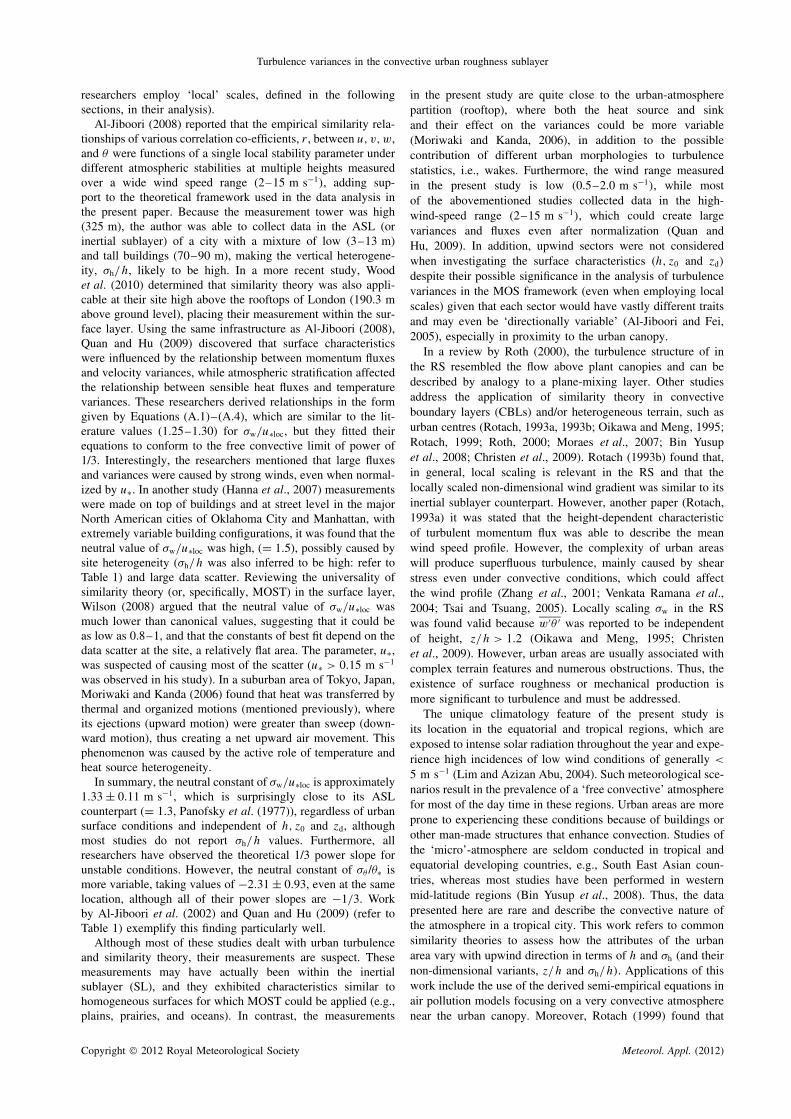
Observations using tower-based meteorological instruments (ata combined height, z = 18 m) were made on the rooftop ofthe School of Industrial Technology, Universiti Sains Malaysia(USM) (5°21′28′′N; 100°18’06.5′′E), Penang, Malaysia. Thesensors were positioned such that they were not obstructedby buildings or trees. The sonic anemometer was installed atz = 18 m from ground level, and the morphometric methodsgiven by Grimmond and Oke (1999) were used to determinethe displacement height, zd, and roughness length, z0 (14 and0.38 m, respectively), which are summed to yield the effectivemeasurement height, z′ = 4 m. Turbulence data were recordedduring the 3 month intermittent observational period fromNovember 2009 to March 2011, during the winter monsoon.The fetch distance was also estimated to be 370 m using therule-of-thumb equation given in Roth (2000).

This sampling location was surrounded by various facilities,including lecture hall complexes and student hostels (Figure 1).Because different sectors have different building structuresand topographies, the surrounding area was divided into foursectors, labelled A, B, C and D, depending on the 30 minaveraged wind direction. The four sectors were also chosen tomaximize the number of data points in each sector. The heightsof the observation site in relation to other buildings for allsectors in the surrounding area were as follows: (z/h)A = 1.20;(z/h)B = 1.16; (z/h)C = 1.24; and (z/h)d = 1.16, where h isthe weighted average of building and tree heights in the sector

(refer to Table 2 for details). Even though the sectors seemedsimilar, they differed by the standard deviation of the obstacleheights (between sector A and B). Thus, B can be consideredmore heterogeneous than A (A has higher obstacle density),while C had a sparser distribution of buildings (but more trees)than A and B. Because z/h is somewhat similar for all sectors,another dimensionless parameter is introduced that varies moresignificantly between different sectors. This parameter is thestandard deviation of obstacle height to the average-weightedheight, termed the vertical heterogeneity, σh/h, and was chosenbecause σh varies more strongly between sectors than h does.The site surface is clearly complex. Thus, u′w′

in part dependson the upwind surface characteristics in this case. Furthermore,the division of a heterogeneous area into sectors is almoststandard practice and is recommended near an urban canopy,such as in the work of Christen et al. (2009) and Grimmondand Oke (1999). Christen et al. (2009) found that u′w′

increasedbased on the crosswind/along-wind direction of flow in relationto a street canyon, while Al-Jiboori and Fei (2005) discoveredthat z0 was considerably direction-dependent over an urbanarea.

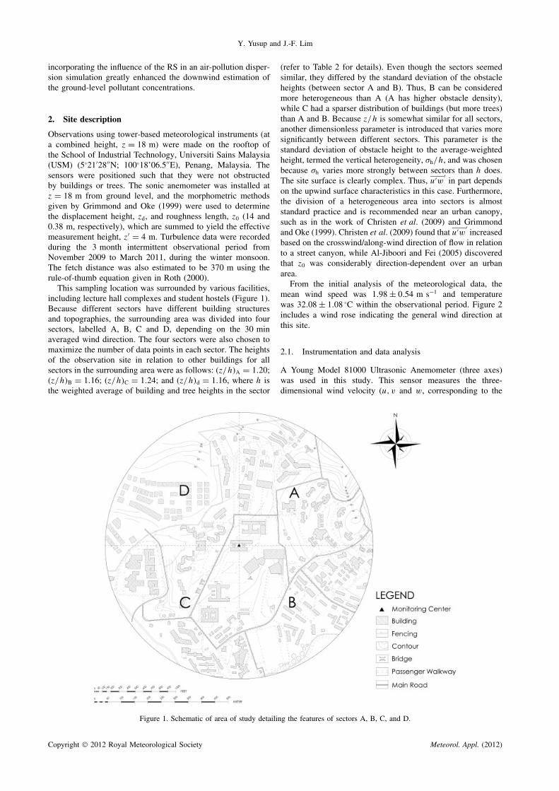
From the initial analysis of the meteorological data, themean wind speed was 1.98 ± 0.54 m s−1 and temperaturewas 32.08 ± 1.08 °C within the observational period. Figure 2includes a wind rose indicating the general wind direction atthis site.

2.1. Instrumentation and data analysis

A Young Model 81000 Ultrasonic Anemometer (three axes)was used in this study. This sensor measures the three-dimensional wind velocity (u, v and w, corresponding to the

Figure 1. Schematic of area of study detailing the features of sectors A, B, C, and D.

Copyright 2012 Royal Meteorological Society Meteorol. Appl. (2012)

Turbulence variances in the convective urban roughness sublayer

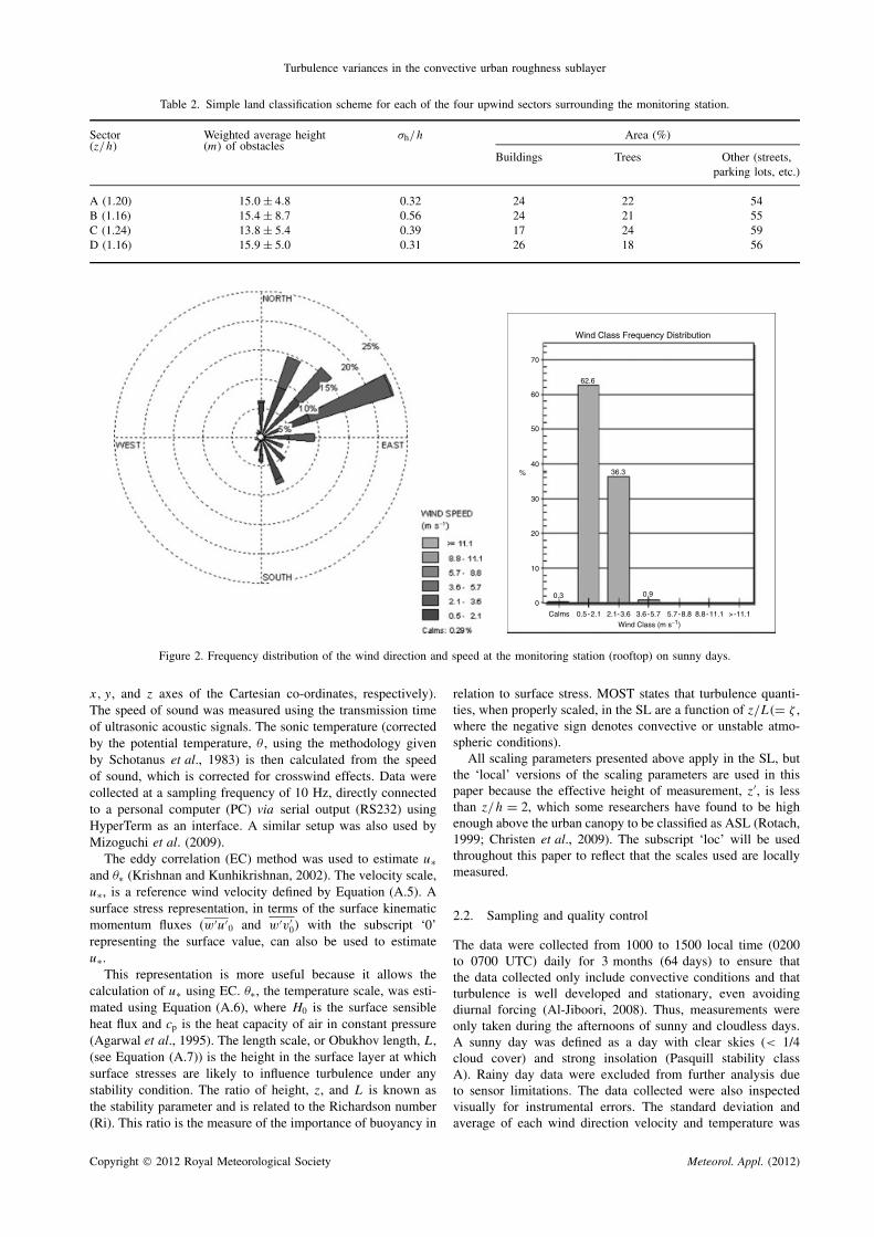
Table 2. Simple land classification scheme for each of the four upwind sectors surrounding the monitoring station.

Sector Weighted average height σh/h Area (%)(z/h) (m) of obstacles

Buildings Trees Other (streets,parking lots, etc.)

A (1.20) 15.0 ± 4.8 0.32 24 22 54B (1.16) 15.4 ± 8.7 0.56 24 21 55C (1.24) 13.8 ± 5.4 0.39 17 24 59D (1.16) 15.9 ± 5.0 0.31 26 18 56

Calms 0.5-2.1 2.1-3.6 3.6-5.7 5.7-8.8 8.8-11.1 >-11.1Wind Class (m s−1)

0.90.3

36.3

62.6

Wind Class Frequency Distribution

70

60

50

40

30

20

10

0

%

Figure 2. Frequency distribution of the wind direction and speed at the monitoring station (rooftop) on sunny days.

x, y, and z axes of the Cartesian co-ordinates, respectively).The speed of sound was measured using the transmission timeof ultrasonic acoustic signals. The sonic temperature (correctedby the potential temperature, θ , using the methodology givenby Schotanus et al., 1983) is then calculated from the speedof sound, which is corrected for crosswind effects. Data werecollected at a sampling frequency of 10 Hz, directly connectedto a personal computer (PC) via serial output (RS232) usingHyperTerm as an interface. A similar setup was also used byMizoguchi et al. (2009).

The eddy correlation (EC) method was used to estimate u∗and θ∗ (Krishnan and Kunhikrishnan, 2002). The velocity scale,u∗, is a reference wind velocity defined by Equation (A.5). Asurface stress representation, in terms of the surface kinematicmomentum fluxes (w′u′

0 and w′v′0) with the subscript ‘0’

representing the surface value, can also be used to estimateu∗.

This representation is more useful because it allows thecalculation of u∗ using EC. θ∗, the temperature scale, was esti-mated using Equation (A.6), where H0 is the surface sensibleheat flux and cp is the heat capacity of air in constant pressure(Agarwal et al., 1995). The length scale, or Obukhov length, L,(see Equation (A.7)) is the height in the surface layer at whichsurface stresses are likely to influence turbulence under anystability condition. The ratio of height, z, and L is known asthe stability parameter and is related to the Richardson number(Ri). This ratio is the measure of the importance of buoyancy in

relation to surface stress. MOST states that turbulence quanti-ties, when properly scaled, in the SL are a function of z/L(= ζ ,where the negative sign denotes convective or unstable atmo-spheric conditions).

All scaling parameters presented above apply in the SL, butthe ‘local’ versions of the scaling parameters are used in thispaper because the effective height of measurement, z′, is lessthan z/h = 2, which some researchers have found to be highenough above the urban canopy to be classified as ASL (Rotach,1999; Christen et al., 2009). The subscript ‘loc’ will be usedthroughout this paper to reflect that the scales used are locallymeasured.

2.2. Sampling and quality control

The data were collected from 1000 to 1500 local time (0200to 0700 UTC) daily for 3 months (64 days) to ensure thatthe data collected only include convective conditions and thatturbulence is well developed and stationary, even avoidingdiurnal forcing (Al-Jiboori, 2008). Thus, measurements wereonly taken during the afternoons of sunny and cloudless days.A sunny day was defined as a day with clear skies (< 1/4cloud cover) and strong insolation (Pasquill stability classA). Rainy day data were excluded from further analysis dueto sensor limitations. The data collected were also inspectedvisually for instrumental errors. The standard deviation andaverage of each wind direction velocity and temperature was

Copyright 2012 Royal Meteorological Society Meteorol. Appl. (2012)

Y. Yusup and J.-F. Lim

computed using block averages and has been found to workwell in stationary conditions (Culf, 2000), which is in the30–45 min range (as suggested by Pasquill and Smith (1983)).Horizontal rotation was also performed on the longitudinal windvelocity component before further analysis. The vertical windcomponent was forced to achieve zero mean, w = 0, (horizontalwind flow) as suggested by Panofsky and Dutton (1984). Themean of the lateral wind component was also forced to bezero, v = 0 (Arya, 1999). However, the obtained values werethe same as the values obtained using a non-zero mean forthe lateral wind component. Vickers and Mahrt’s (1997) dataquality control methodology was applied to the collected datato ensure the quality of the calculated turbulent fluxes andvariances.

The block averages or record length, Rl , must be properlychosen to ensure the accurate calculation of w′θ ′, w′u′, and w′v′and, consequently, u∗. The methodology suggested by Vickersand Mahrt (1997) was used to determine Rl . The relativesystematic flux error (RSE) test was performed on the datato check for flux underestimation caused by an inappropriatechoice of Rl . RSE tests were performed for three recordlengths: 5, 30 and 60 min. The results of these tests indicatethat Rl = 5 min underestimated the fluxes, while Rl = 60 minproduced the same results as Rl = 30 min. Thus, a recordlength of 30 min was chosen for this study. This time pointwas also recommended by Pasquill and Smith (1983) andPanofsky and Dutton (1984) and used in an urban settingby Roth et al. (2006) and Bin Yusup et al. (2008), althoughsome authors have used shorter durations in similar settings(Oikawa and Meng, 1995). It is interesting to note that Wilson(2008) tentatively determined that the averaging time was notimportant in determining the neutral limit of σw/u∗.

Four types of nonstationarity tests were applied to the data.Nonstationary conditions can affect the fluxes estimated by EC.As outlined by Vickers and Mahrt (1997), the four tests werethe wind speed reduction, along-wind relative non-stationarity(RNu), crosswind relative non-stationarity (RNv), and vector-wind relative non-stationarity (RNS) tests. The collected datawere determined to be nonstationary for 11% of the data.However, non-stationary data do not significantly increase thescattering of the variances and fluxes within certain rangesof atmospheric stability (2 > ζ > −3), as shown by MarquesFilho et al. (2008).

3. Results and discussion

3.1. General description of processed turbulence data

The observed standard deviations of the u, v and w windvelocity components are summarized in Table 3. Bin Yusupet al. (2008) performed a similar study across the strait from thissite in the nearby heavy industrial area of Prai (approximately10 km away). Higher values of σu and σv but lower values forσw were observed in the present study compared to those byBin Yusup et al. (2008) due to the presence of more surfaceobstacles in this site, which mainly affects the horizontal windcomponents. In addition, the average and median values ofσu and σv were equal for this site. As mentioned above, themeasurements were taken from mostly low-wind-speed (<3 m s−1) conditions for which large standard deviations arecommon. The number of data sets (Ntotal = 574), N , for eachatmospheric stability class observed was distributed as follows(where z′/Lloc = ζloc):

Table 3. Daytime (convective conditions) arithmetic mean and medianof field experiment conditions.

Parameters Present study(N = 574)

Bin Yusup et al. (2008)(N = 80)

Mean Median Mean Median

z′ (m) 4 – 2 –V (m s−1) 1.97 ± 0.54 198 1.82 ± 0.85 1.87U∗loc (m s−1) 0.27 ± 0.09 0.28 0.31 ± 0.20 0.36w′θ ′ 0.11 ± 0.04 0.11 – –|Lloc| (m) 20 ± 17 17 – –σu (m s−1) 1.54 ± 0.41 1.54 0.91 ± 0.24 0.96σv (m s−1) 1.54 ± 0.42 1.53 0.80 ± 0.15 0.82σw (m s−1) 0.41 ± 0.11 0.40 0.65 ± 0.18 0.68σθ (°C) 0.74 ± 0.17 0.77 – –

1. −0.01 > ζloc > −0.1, N = 652. −0.1 > ζloc > −1, N = 4213. −1 > ζloc > −10, N = 864. ζloc < −10, N = 2

The prevalent unstable atmospheric state was anticipatedbecause the observations were made in the afternoon.

The numbers of data categorized (based on wind direction)into sectors A, B, C and D were 290, 176, 88 and 20,respectively. The data in sectors C and D were not analysedfurther due to a lack of data and the occurrence of non-stationary conditions (wind meandering caused by very lowwind speeds, < 1 m s−1, evident in Figure 2 for sector C).Higher-order moments of θ also indicated that there manyoccurrences of skewness and kurtosis (soft-flagged) for θ (14and 4% of the data, respectively) and kurtosis for u (3%) insector C, whereas the incidences of kurtosis and skewnessof u, v and θ for sectors A and B were low (2–3%).Thus, the analysed data describe turbulence originating fromupwind characteristics of similar average-weighted heights, h,but different standard deviation of obstacle heights, σh, forsectors A and B (refer to Table 2), for which the effect of thedimensionless heights, z/h and σh/h, and can be tested on σw

and σθ .Because measurements were made on the rooftop of a build-

ing, the collected data represent turbulence characteristic withinthe RS. However, the concept of local scaling (locally measuredparameters) is still predicted to hold true in the roughness sub-layer (Hogstrom et al., 1982) and was demonstrated by Oikawaand Meng (1995) and other authors (Rotach, 1999; Moriwakiand Kanda, 2006). This concept will be applied to the verti-cal wind velocity component and temperature and should beadequately described by this concept, in contrast to the hori-zontal wind component (Rotach, 1993a). Christen et al. (2009)has cautioned that this approach could be inadequate for flowwithin the RS (in street canyons) and the near-roofs vicinity.However, their study primarily dealt with near-neutral atmo-spheric conditions.

3.2. Correlation between u–v and w–θ

Several studies have determined that the condition when sur-face layer scaling or its equivalent is applicable is definedby a stationary, homogeneous terrain and a high correlationbetween w–θ and u–v of generally r > 0.5. Kaimal and Finni-gan (1994) observed that in the surface layer, the correlationwas approximately 0.5 (0 > ζ > −2) between w and θ and

Copyright 2012 Royal Meteorological Society Meteorol. Appl. (2012)

Turbulence variances in the convective urban roughness sublayer

approximately −0.35 (1 > ζ > −1) between u and v. Our cor-relation was generally lower than these ranges, e.g., 0.56 >

rwθ > 0.13 and 3.32 × 10−2 > −ruv > 1.73 × 10−4. The aver-ages were rwθ = 0.38 and −ruv = 0.011. The low correlationof u–v can be attributed to the many obstacles located upwind.Similarly, an even lower average of correlation for w–θ inunstable conditions (= 0.24) and large scattering of the cor-relation for u–v were obtained by Al-Jiboori (2008), despitesimilarity theory using local scales being applicable at his site.A check of the turbulent intensity, Iw = σw/V , showed thatit had an average of 0.22 where Taylor’s frozen hypothesis(Iw < 0.5) still holds (Agarwal et al., 1995). However, it wasfound that Iu and Iv were larger than 0.5.

3.3. Scaling σw using u∗loc in RS

The normalized standard deviations of w and θ throughoutthe observational period are plotted against the atmosphericstability parameter, ζloc. These plots enable derivation of semi-empirical equations that relate the aforementioned turbulentstatistics with ζloc when properly scaled. Moraes (2000) men-tioned that significant scatter in these plots indicates that thescaling parameters used are inadequate, causing the turbulencefluxes to depend on other parameters. Simple power law equa-tions were used to fit σw/u∗loc, as done by Kader and Yaglom(1990), and the equation in the form made popular by Panofskyand Dutton (1984) was used to fit σθ /θ∗loc. The data were fittedusing the Matlab 2008a curve fitting tool, more specificallythe least square regression scheme. The form of the equationused was based on the R2 obtained, in favour of a value nearunity.

Figure 3(a) and (b), for sectors A and B clearly showthat σw/u∗loc is a function of (−ζloc)

1/3 for very convectiveconditions starting at approximately ζloc = −0.3 (R2

wA = 0.78for A and R2

wB = 0.86 for B) (Oikawa and Meng, 1995), whichagrees with predictions, although Arya (1999) suggested thatthe increase should start below −0.5. Above ζloc = −0.5, thedata were more scattered because upwind surface heterogeneitycaused scatter in the variable u∗loc despite its generally largervalue compared to when ζloc < −0.5. Oikawa and Meng (1995)found that the magnitude of the normalized standard deviationswas systematically higher within the canopy, suggesting thatthe values obtained for sector B were within the ‘urban layercanopy’. However, this conclusion contradicts that drawn byRoth (2000).

From these results, the semi-empirical equations derived arevalid for σw/u∗loc and can be written as Equations (1) and (2),which exhibit a reasonably good fit (Figure 3).

Hogstrom et al. (1982) suggested, and Rotach (1993a) laterdemonstrated, that locally scaled σw can be related to ζloc in theURS in the same fashion as scaling in the ASL. The equationgiven by Panofsky et al. (1977) is similar to the equationthat describes the data in sectors A and B. A side-by-sidecomparison of the equations in the form of Equation (2) is alsoprovided in Figure 3:

(σw

u∗loc

)A

= 1.04(1 − 5.38ζloc)0.32, R2

wA = 0.78 (1)

(σw

u∗loc

)B

= 1.27(1 − 5.31ζloc)0.29, R2

wB = 0.86 (2)

(note: for −0.01 > ζloc > −100).This phenomenon is well documented in the literature

(Panofsky and Dutton, 1984; Krishnan and Kunhikrishnan,

(a)

(b)

Figure 3. The σw/u∗loc distribution with −ζloc(−0.01 > ζloc > −20)and sectors using a log-log scale for better visualization of the 1/3power trend (dashed line). The vertical dashed line denotes ζloc = −0.3,and the vertical dot-dot line denotes ζloc = −0.5. The solid lines are

based on Equations (1)–(2) for sectors A (a) and B (b).

2002; von Randow et al., 2006), although very convective con-ditions, −0.01 > −ζ > −100, are rarely reported, especially inequatorial cities (Krishnan and Kunhikrishnan, 2002; Bin Yusupet al., 2008). The near-neutral constant obtained as the neu-tral value extrapolated from Equations (1) and (2) was higher(= 1.44, an averaged value) than that used in the equation forσw/u∗ by Bin Yusup et al. (2008), although there is insuf-ficient data in the near-neutral range to confirm this result.However, Roth (2000) stated that ζ > −0.05 could still beconsidered near-neutral, at least for sector A. Similar resultsto Bin Yusup et al. (2008) should be expected because bothobservational stations were near one another. Any deviationwas caused by the sensor and sampling frequency used, whichlimits the flux-capture capability of the 1 Hz propeller-basedanemometer used by Bin Yusup et al. (2008). Another possi-ble factor was the difference in local topography or terrain andthe atmospheric stability range, which the authors measured asonly 0 > ζ > −2.

The upwind surface characteristic could play a role inthe difference in results between sectors A and B, althoughZhang et al. (2001) mentioned that the vertical wind velocityis influenced by small high-frequency eddies and are able toadapt immediately to a new terrain, thus explaining its goodrelationship with −ζ , even in complex terrains. As shown inTable 2, the average height of obstacles and the area covered in

Copyright 2012 Royal Meteorological Society Meteorol. Appl. (2012)

Y. Yusup and J.-F. Lim

sectors A and B were somewhat similar (< 3% for z/h betweensectors) and similarly ‘homogeneous’ given that the percentageof area covered by buildings, trees and other obstacles areidentical. Thus, this observation raises the question: why dothe best-fit lines for σw/u∗loc differ for these sectors?

The answer lies in the dimensionless σh/h, which differsby approximately 75%. Al-Jiboori and Fei (2005) found thatchanges in the general wind direction (thus, upwind surfacecharacteristics) cause large disparities in the observed values ofconstants. Hanna et al. (2007) also mentioned that the presenceof obstacles (or buildings) would produce an increase in thehorizontal fluctuations caused by the wake of these obstaclesthat differ in size and/or position. In the present study, thisdifference manifests itself in the different values for σh/h: 1.04in Equation (1) for sector A and 1.27 in Equation (2) for sectorB. A lower constant value was explained by Moriwaki andKanda (2006), who attributed it to the rough feature of the urbansurface, which better facilitates momentum transport comparedto flatter surfaces. Roth (2000) stated that any deviation fromequations and constants obtained in the SL are due to smallernon-dimensional dissipation values for turbulent kinetic energy(TKE) because energy is introduced into the TKE budgetfrom local sources (local production > local dissipation),i.e., vertical transport, flux divergence, pressure transport andhorizontal advection. Poggi et al. (2004) found that sparsecanopies exhibited higher near-neutral σw/u∗ values (≈ 1.3)than its denser counterpart (≈ 1.1), which was observed using alaboratory-scale channelled flow setup on uniformly distributedobstacles (or rods) of equal height. This conclusion is alsosupported by Raupach et al. (1996). Both studies are for flowover vegetated canopies: these canopies have strong similaritieswith the urban canopy, while sparse canopies require additionalMOS modifications to be interpreted in the same framework dueto the increasing importance of turbulence generated by wakes(Roth, 2000). Referring back to sectors A and B, because aerialobstacle densities are similar for both sectors, the changes inσh/h affect these constants (by 22%) just as they would density.Nevertheless, Equations (1) and (2) show behaviour expectedfrom local scaling and, by extension, surface layer scaling,further supporting the work by Rotach (1993a).

3.3.1. Spectral analysis of w

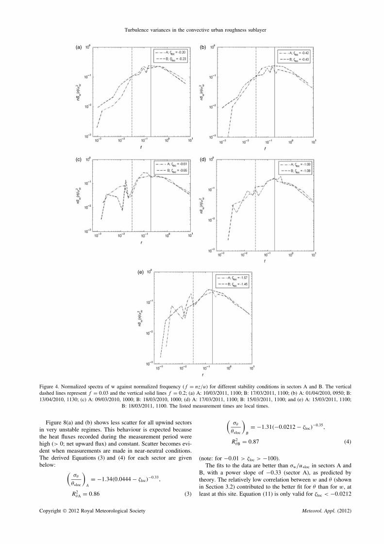
The spectral analysis of the normalized w component for a datablock of 30 min following the procedure detailed in Kaimalet al. (1972) revealed that the difference between sectors Aand B became discernible in the normalized low-frequencyrange f (= nz/V ) < 0.03, while the spectral-peak-normalizedfrequency (f = 0.2; f = 0.1 from Roth (2000)) remained thesame. However, other researchers have observed that the w-spectra have lower frequency offsets at neutral and unstableconditions (Roth, 2000), the overall curves look similar tothe ASL predictions (Kaimal et al., 1972). The latter authormentioned that a displacement of peak frequencies would beexpected for significant wake length scales, but in the contextof the present paper, the spectral power is displaced (upwardsfor sector B) and only for f < 0.03 and ζloc > −0.6 due to thedifferent σh/h. The −2/3 power slope in the inertial subrangeis obvious for both sectors and all instability conditionsmeasured. A trend was also observed in which the spectralpower increases in value as atmospheric stability decreases(Figure 4). The results of spectral analysis corroborate thelower constant values from the best-fit curves obtained forsector A (with lower σh/h) compared to sector B until beyondζloc = −0.6, where the difference becomes less apparent (see

Figure 5). Under very unstable conditions, the turbulence in theurban canopy would also involve eddies created by ‘thermalplumes’ or ‘downdraughts’, which are more prevalent thanwake contributions or σh/h, originating from heat sources andsinks on the urban surface. Al-Jiboori (2008) showed thatwhen ζloc < −0.7, the correlation co-efficient, rwθ , increased to0.24, revealing the atmospheric condition when the transitionfrom mechanically to convectively driven (free convection)turbulence occurs in the urban roughness sublayer, which isalso seen in this study but in the layer directly above the urbancanopy. However, it is important to note that at higher unstableconditions, the momentum and heat sources and sinks in theimmediate vicinity have a stronger influence on its fluxes (Roth,2000).

A figure by Oikawa and Meng (1995) (fig. 6 in theirpaper) also displays this trend for different z values, wherethe spectral power decreases more rapidly when lower thanf = 0.03 at z = 18 m than at z = 5.4 m. The authors noticed‘dips’ and concluded that it was due to ‘organized motions’,more specifically, sweeps and ejection. Using quadrant analysissimilar to that employed by Oikawa and Meng (1995), it wasdetermined that ejection motion dominates for both sectors Aand B (results not reported here). This figure also showed asystematic separation of spectral power directly after the dip.In the present study, the natural frequency of 0.03 Hz (wherethe dip for ζloc < −0.6 and separation occur) correspondsto 33 s, which refers to large-scale motions associated withReynolds stress production. Thus, the vertical heterogeneity(σh/h) of the different sectors A (less heterogeneous) and Baffects the normalized σw by increasing its overall value at lowatmospheric instability ζloc > −0.20, just as it would at differentmeasurement heights above the rooftop canopy due to dips andseparation in the low-frequency range (large-scale motions).

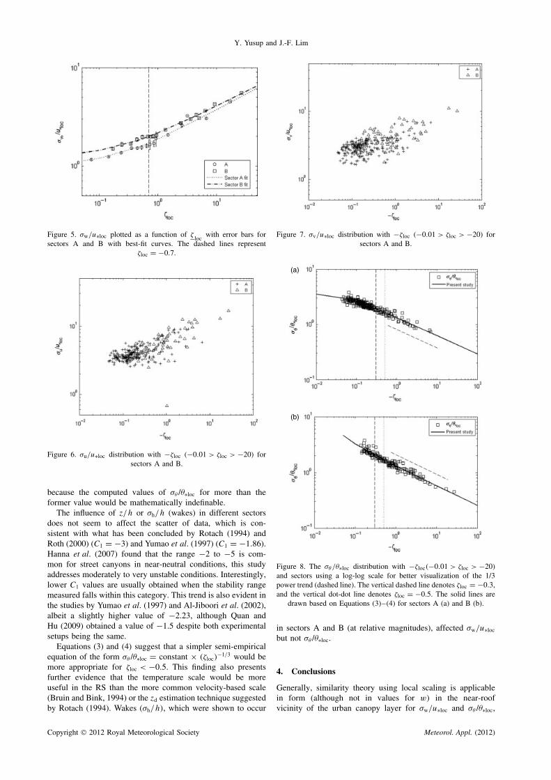
3.4. Turbulence statistics of σu and σv with ζloc

in the RS

Similarity theory normally does not apply for u and v (evenin the homogeneous surface layer), unlike w (please refer toFigures 6 and 7: the data are more scattered) (Rotach, 1993a;Moraes et al., 2007). In addition, the fact that turbulent intensityfor u and w exceeded 0.5 and the low correlation between u andv, as mentioned in Section 3.2, indicates that Taylor’s frozenhypothesis was not applicable for this situation. Thus, inter-preting the data in the framework of similarity theory wouldbe even more unfounded. Nevertheless, the observations sug-gest that surface roughness and terrain complexity influence theturbulent fluxes and their relationship to the stability parame-ter for σw when σh/h is high, causing wake developments thataffect the empirical constants by increasing their values whenapproaching near-neutral conditions from ζloc > −0.6 onwards.

3.5. Scaling σθ using θ∗loc in the RS

As stated in the Introduction, Equations (A.3) and (A.4) suggestthat σθ /θ∗ with −ζ will obey the −1/3 power law underunstable or convective condition. This research supports thistheory. The data were fitted using the form of the expressionshown in Equation (A.4) (Tillman, 1972), where C1 and C2

are constants, based on the R2 value. It is important to notethat extrapolation to near-neutral values is solely dependent onthe best-fit equation obtained and not the measured data, thuscreating the possibility that other equation forms could be moresuitable for 0 > ζ > −0.01.

Copyright 2012 Royal Meteorological Society Meteorol. Appl. (2012)

Turbulence variances in the convective urban roughness sublayer

(a) (b)

(c)

(e)

(d)

Figure 4. Normalized spectra of w against normalized frequency (f = nz/u) for different stability conditions in sectors A and B. The verticaldashed lines represent f = 0.03 and the vertical solid lines f = 0.2; (a) A: 10/03/2011, 1100; B: 17/03/2011, 1100; (b) A: 01/04/2010, 0950; B:13/04/2010, 1130; (c) A: 09/03/2010, 1000; B: 18/03/2010, 1000; (d) A: 17/03/2011, 1100; B: 15/03/2011, 1100; and (e) A: 15/03/2011, 1100;

B: 18/03/2011, 1100. The listed measurement times are local times.

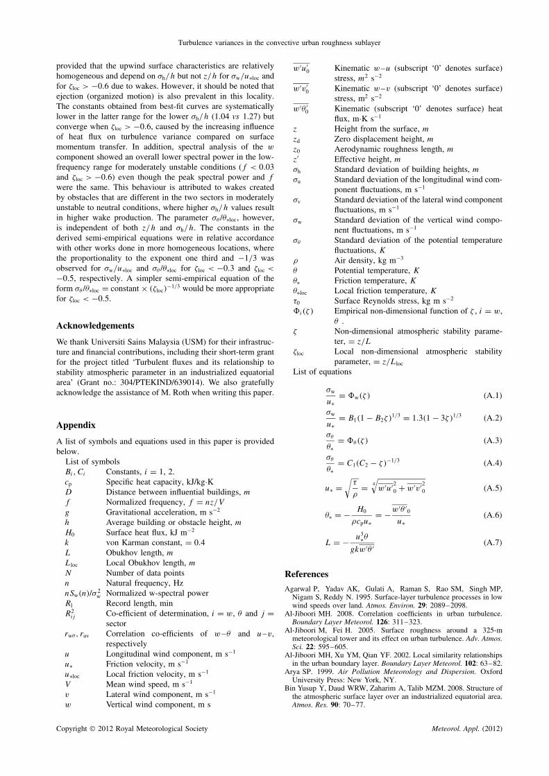
Figure 8(a) and (b) shows less scatter for all upwind sectorsin very unstable regimes. This behaviour is expected becausethe heat fluxes recorded during the measurement period werehigh (> 0; net upward flux) and constant. Scatter becomes evi-dent when measurements are made in near-neutral conditions.The derived Equations (3) and (4) for each sector are givenbelow: (

σθ

θ∗loc

)A

= −1.34(0.0444 − ζloc)−0.33,

R2θA = 0.86 (3)

(σθ

θ∗loc

)B

= −1.31(−0.0212 − ζloc)−0.35,

R2θB = 0.87 (4)

(note: for −0.01 > ζloc > −100).The fits to the data are better than σw/u∗loc in sectors A and

B, with a power slope of −0.33 (sector A), as predicted bytheory. The relatively low correlation between w and θ (shownin Section 3.2) contributed to the better fit for θ than for w, atleast at this site. Equation (11) is only valid for ζloc < −0.0212

Copyright 2012 Royal Meteorological Society Meteorol. Appl. (2012)

Y. Yusup and J.-F. Lim

Figure 5. σw/u∗loc plotted as a function of ζloc

with error bars forsectors A and B with best-fit curves. The dashed lines represent

ζloc = −0.7.

Figure 6. σu/u∗loc distribution with −ζloc (−0.01 > ζloc > −20) forsectors A and B.

because the computed values of σθ /θ∗loc for more than theformer value would be mathematically indefinable.

The influence of z/h or σh/h (wakes) in different sectorsdoes not seem to affect the scatter of data, which is con-sistent with what has been concluded by Rotach (1994) andRoth (2000) (C1 = −3) and Yumao et al. (1997) (C1 = −1.86).Hanna et al. (2007) found that the range −2 to −5 is com-mon for street canyons in near-neutral conditions, this studyaddresses moderately to very unstable conditions. Interestingly,lower C1 values are usually obtained when the stability rangemeasured falls within this category. This trend is also evident inthe studies by Yumao et al. (1997) and Al-Jiboori et al. (2002),albeit a slightly higher value of −2.23, although Quan andHu (2009) obtained a value of −1.5 despite both experimentalsetups being the same.

Equations (3) and (4) suggest that a simpler semi-empiricalequation of the form σθ /θ∗loc = constant × (ζloc)

−1/3 would bemore appropriate for ζloc < −0.5. This finding also presentsfurther evidence that the temperature scale would be moreuseful in the RS than the more common velocity-based scale(Bruin and Bink, 1994) or the zd estimation technique suggestedby Rotach (1994). Wakes (σh/h), which were shown to occur

Figure 7. σv/u∗loc distribution with −ζloc (−0.01 > ζloc > −20) forsectors A and B.

(a)

(b)

Figure 8. The σθ /θ∗loc distribution with −ζloc(−0.01 > ζloc > −20)and sectors using a log-log scale for better visualization of the 1/3power trend (dashed line). The vertical dashed line denotes ζloc = −0.3,and the vertical dot-dot line denotes ζloc = −0.5. The solid lines are

drawn based on Equations (3)–(4) for sectors A (a) and B (b).

in sectors A and B (at relative magnitudes), affected σw/u∗loc

but not σθ /θ∗loc.

4. Conclusions

Generally, similarity theory using local scaling is applicablein form (although not in values for w) in the near-roofvicinity of the urban canopy layer for σw/u∗loc and σθ /θ∗loc,

Copyright 2012 Royal Meteorological Society Meteorol. Appl. (2012)

Turbulence variances in the convective urban roughness sublayer

provided that the upwind surface characteristics are relativelyhomogeneous and depend on σh/h but not z/h for σw/u∗loc andfor ζloc > −0.6 due to wakes. However, it should be noted thatejection (organized motion) is also prevalent in this locality.The constants obtained from best-fit curves are systematicallylower in the latter range for the lower σh/h (1.04 vs 1.27) butconverge when ζloc > −0.6, caused by the increasing influenceof heat flux on turbulence variance compared on surfacemomentum transfer. In addition, spectral analysis of the w

component showed an overall lower spectral power in the low-frequency range for moderately unstable conditions (f < 0.03and ζloc > −0.6) even though the peak spectral power and f

were the same. This behaviour is attributed to wakes createdby obstacles that are different in the two sectors in moderatelyunstable to neutral conditions, where higher σh/h values resultin higher wake production. The parameter σθ /θ∗loc, however,is independent of both z/h and σh/h. The constants in thederived semi-empirical equations were in relative accordancewith other works done in more homogeneous locations, wherethe proportionality to the exponent one third and −1/3 wasobserved for σw/u∗loc and σθ /θ∗loc for ζloc < −0.3 and ζloc <

−0.5, respectively. A simpler semi-empirical equation of theform σθ /θ∗loc = constant × (ζloc)

−1/3 would be more appropriatefor ζloc < −0.5.

Acknowledgements

We thank Universiti Sains Malaysia (USM) for their infrastruc-ture and financial contributions, including their short-term grantfor the project titled ‘Turbulent fluxes and its relationship tostability atmospheric parameter in an industrialized equatorialarea’ (Grant no.: 304/PTEKIND/639014). We also gratefullyacknowledge the assistance of M. Roth when writing this paper.

Appendix

A list of symbols and equations used in this paper is providedbelow.

List of symbolsBi, Ci Constants, i = 1, 2.cp Specific heat capacity, kJ/kg·KD Distance between influential buildings, m

f Normalized frequency, f = nz/V

g Gravitational acceleration, m s−2

h Average building or obstacle height, m

H0 Surface heat flux, kJ m−2

k von Karman constant, = 0.4L Obukhov length, m

Lloc Local Obukhov length, m

N Number of data pointsn Natural frequency, HznSw(n)/σ 2

w Normalized w-spectral powerRl Record length, minR2

ij Co-efficient of determination, i = w, θ and j =sector

rwθ , ruv Correlation co-efficients of w–θ and u–v,respectively

u Longitudinal wind component, m s−1

u∗ Friction velocity, m s−1

u∗loc Local friction velocity, m s−1

V Mean wind speed, m s−1

v Lateral wind component, m s−1

w Vertical wind component, m s

w′u′0 Kinematic w–u (subscript ‘0’ denotes surface)

stress, m2 s−2

w′v′0 Kinematic w–v (subscript ‘0’ denotes surface)

stress, m2 s−2

w′θ ′0 Kinematic (subscript ‘0’ denotes surface) heat

flux, m·K s−1

z Height from the surface, m

zd Zero displacement height, m

z0 Aerodynamic roughness length, m

z′ Effective height, m

σh Standard deviation of building heights, m

σu Standard deviation of the longitudinal wind com-ponent fluctuations, m s−1

σv Standard deviation of the lateral wind componentfluctuations, m s−1

σw Standard deviation of the vertical wind compo-nent fluctuations, m s−1

σθ Standard deviation of the potential temperaturefluctuations, K

ρ Air density, kg m−3

θ Potential temperature, K

θ∗ Friction temperature, K

θ∗loc Local friction temperature, K

τ0 Surface Reynolds stress, kg m s−2

�i(ζ ) Empirical non-dimensional function of ζ , i = w,θ .

ζ Non-dimensional atmospheric stability parame-ter, = z/L

ζloc Local non-dimensional atmospheric stabilityparameter, = z/Lloc

List of equations

σw

u∗= �w(ζ ) (A.1)

σw

u∗= B1(1 − B2ζ )1/3 = 1.3(1 − 3ζ )1/3 (A.2)

σθ

θ∗= �θ(ζ ) (A.3)

σθ

θ∗= C1(C2 − ζ )−1/3 (A.4)

u∗ =√

τ

ρ= 4

√w′u′2

0 + w′v′20 (A.5)

θ∗ = − H0

ρcpu∗= −w′θ ′

0

u∗(A.6)

L = − u3∗θ

gkw′θ ′ (A.7)

References

Agarwal P, Yadav AK, Gulati A, Raman S, Rao SM, Singh MP,Nigam S, Reddy N. 1995. Surface-layer turbulence processes in lowwind speeds over land. Atmos. Environ. 29: 2089–2098.

Al-Jiboori MH. 2008. Correlation coefficients in urban turbulence.Boundary Layer Meteorol. 126: 311–323.

Al-Jiboori M, Fei H. 2005. Surface roughness around a 325-mmeteorological tower and its effect on urban turbulence. Adv. Atmos.Sci. 22: 595–605.

Al-Jiboori MH, Xu YM, Qian YF. 2002. Local similarity relationshipsin the urban boundary layer. Boundary Layer Meteorol. 102: 63–82.

Arya SP. 1999. Air Pollution Meteorology and Dispersion. OxfordUniversity Press: New York, NY.

Bin Yusup Y, Daud WRW, Zaharim A, Talib MZM. 2008. Structure ofthe atmospheric surface layer over an industrialized equatorial area.Atmos. Res. 90: 70–77.

Copyright 2012 Royal Meteorological Society Meteorol. Appl. (2012)

Y. Yusup and J.-F. Lim

Bruin HAR, Bink NJ. 1994. The use of σT as a temperature scale inthe atmospheric surface layer. Boundary Layer Meteorol. 70: 79–93.

Christen A, Rotach MW, Vogt R. 2009. The budget of turbulent kineticenergy in the urban roughness sublayer. Boundary Layer Meteorol.131: 193–222.

Culf AD. 2000. Examples of the effects of different averaging methodson carbon dioxide fluxes calculated using the eddy correlationmethod, HAL – CCSD.

Foken T. 2006. 50 years of the Monin-Obukhov similarity theory.Boundary Layer Meteorol. 119: 431–447.

Grimmond CSB, Oke TR. 1999. Aerodynamic properties of urbanareas derived, from analysis of surface form. J. Appl. Meteorol. 38:1262–1292.

Hanna S, White J, Zhou Y. 2007. Observed winds, turbulence, anddispersion in built-up downtown areas of Oklahoma City andManhattan. Boundary Layer Meteorol. 125: 441–468.

Hicks BB. 1981. An examination of turbulence statistics in the surfaceboundary layer. Boundary Layer Meteorol. 21: 389–402.

Hogstrom U, Bergstrom H, Alexandersson H. 1982. Turbulencecharacteristics in a near neutrally stratified urban atmosphere.Boundary Layer Meteorol. 23: 449–472.

Hurk BJJM, Bruin HAR. 1995. Fluctuations of the horizontal windunder unstable conditions. Boundary Layer Meteorol. 74: 341–352.

Kader BA, Yaglom AM. 1990. Mean fields and fluctuation momentsin unstably stratified turbulent boundary layers. J. Fluid Mech. 212:637–662.

Kaimal JC, Finnigan JJ. 1994. Atmospheric Boundary Layer Flows:Their Structure and Measurement. Oxford University Press: NewYork, NY.

Kaimal JC, Wyngaard JC, Izumi Y, Cote OR. 1972. Spectral char-acteristics of surface-layer turbulence. Q. J. R. Meteorol. Soc. 98:563–589.

Krishnan P, Kunhikrishnan PK. 2002. Some characteristics ofatmospheric surface layer over a tropical inland region duringsouthwest monsoon period. Atmos. Res. 62: 111–124.

Lim JT, Azizan Abu S. 2004. Weather and Climate of Malaysia.University of Malaya Press: Kuala Lumpur.

Marques Filho EP, S LDA, Karam HA, Alval RCS, Souza A,Pereira MMR. 2008. Atmospheric surface layer characteristics ofturbulence above the Pantanal wetland regarding the similaritytheory. Agric. For. Meteorol. 148: 883–892.

Mizoguchi Y, Miyata A, Ohtani Y, Hirata R, Yuta S. 2009. A reviewof tower flux observation sites in Asia. J. For. Res. 14: 1–9.

Moraes OLL. 2000. Turbulence characteristics in the surface boundarylayer over the South American Pampa. Boundary Layer Meteorol.96: 317–335.

Moraes OLL, Acevedo O, Martins CA, Anabor V, Degrazia G, daSilva R, Anfossi D. 2007. Analyzing the validity of similaritytheories in complex topographies. Air Pollution Modeling and itsApplications XVII 17: 608–614.

Moriwaki R, Kanda M. 2006. Local and global similarity in turbulenttransfer of heat, water vapour, and CO2 in the dynamic convectivesublayer over a suburban area. Boundary Layer Meteorol. 120:163–179.

Oikawa S, Meng Y. 1995. Turbulence characteristics and organizedmotion in a suburban roughness sublayer. Boundary Layer Meteorol.74: 289–312.

Panofsky HA, Dutton JA. 1984. Atmospheric Turbulence: Models andMethods for Engineering Applications. John Wiley & Sons: NewYork, NY.

Panofsky H, Tennekes H, Lenschow D, Wyngaard J. 1977. Thecharacteristics of turbulent velocity components in the surfacelayer under convective conditions. Boundary Layer Meteorol. 11:355–361.

Pasquill F, Smith FB. 1983. Atmospheric Diffusion. E. Horwood,Halsted Press: Chichester, New York, NY.

Poggi D, Porporato A, Ridolfi L, Albertson JD, Katul GG. 2004.The effect of vegetation density on canopy sub-layer turbulence.Boundary Layer Meteorol. 111: 565–587.

Quan LH, Hu F. 2009. Relationship between turbulent flux andvariance in the urban canopy. Meteorol. Atmos. Phys. 104: 29–36.

von Randow C, Kruijt B, Holtslag AAM. 2006. Low-frequencymodulation of the atmospheric surface layer over Amazonian rainforest and its implication for similarity relationships. Agric. For.Meteorol. 141: 192–207.

Raupach MR, Finnigan JJ, Brunei Y. 1996. Coherent eddies andturbulence in vegetation canopies: the mixing-layer analogy.Boundary Layer Meteorol. 78: 351–382.

Rotach MW. 1993a. Turbulence close to a rough urban surface part I:reynolds stress. Boundary Layer Meteorol. 65: 1–28.

Rotach MW. 1993b. Turbulence close to a rough urban surface part II:variances and gradients. Boundary Layer Meteorol. 66: 75–92.

Rotach MW. 1994. Determination of the zero plane displacement in anurban environment. Boundary Layer Meteorol. 67: 187–193.

Rotach MW. 1999. On the influence of the urban roughness sublayeron turbulence and dispersion. Atmos. Environ. 33: 4001–4008.

Rotach MWL, Vogt R, Bernhofer C, Batchvarova E, Christen A, Clap-pier A, Feddersen B, Gryning SE, Martucci G, Mayer H, Mitev V,Oke TR, Parlow E, Richner H, Roth M, Roulet YA, Ruffieux D,Salmond JA, Schatzmann M, Voogt JA. 2005. BUBBLE – an urbanboundary layer meteorology project. Theor. Appl. Climatol. 81:231–261.

Roth M. 2000. Review of atmospheric turbulence over cities. Q. J. R.Meteorol. Soc. 126: 941–990.

Roth M, Salmond JA, Satyanarayana ANV. 2006. Methodologicalconsiderations regarding the measurement of turbulent fluxes inthe urban roughness sublayer: the role of scintillometery. BoundaryLayer Meteorol. 121: 351–375.

Schotanus P, Nieuwstadt FTM, Bruin HAR. 1983. Temperaturemeasurement with a sonic anemometer and its application to heatand moisture fluxes. Boundary Layer Meteorol. 26: 81–93.

Tillman JE. 1972. The indirect determination of stability, heat andmomentum fluxes in the atmospheric boundary layer from simplescalar variables during dry unstable conditions. J. Appl. Meteorol.11: 783–792.

Tsai J-L, Tsuang B-J. 2005. Aerodynamic roughness over an urban areaand over two farmlands in a populated area as determined by windprofiles and surface energy flux measurements. Agric. For. Meteorol.132: 154–170.

Venkata Ramana M, Krishnan P, Kunhikrishnan PK. 2004. Surfaceboundary-layer characteristics over a tropical inland station: seasonalfeatures. Boundary Layer Meteorol. 111: 153–157.

Vickers D, Mahrt L. 1997. Quality control and flux sampling problemsfor tower and aircraft data. J. Atmos. Oceanic Technol. 14:512–526.

Wilson JD. 2008. Monin-Obukhov functions for standard deviations ofvelocity. Boundary Layer Meteorol. 129: 353–369.

Wood CR, Lacser A, Barlow JF, Padhra A, Belcher SE, Nemitz E,Helfter C, Famulari D, Grimmond CSB. 2010. Turbulent flow at190 m height above London during 2006–2008: a climatology andthe applicability of similarity theory. Boundary Layer Meteorol. 137:77–96.

Yumao XU, Chaofu Z, Zhongkai LI, Wei Z. 1997. Turbulent structureand local similarity in the tower layer over the Nanjing area.Boundary Layer Meteorol. 82: 1–21.

Zhang H, Chen J, Park S-U. 2001. Turbulence structure in unstableconditions over various surfaces. Boundary Layer Meteorol. 100:243–261.

Copyright 2012 Royal Meteorological Society Meteorol. Appl. (2012)