Power Spectral Measurements of Clear-Air Turbulence

TECH LIBRARY WFB, NM

NASA Technical Paper 1979

1982

National Aeronautics and Space Adminstration

Scientific and Technical Information Branch

Power Spectral Measurements of Clear-Air Turbulence to Long Wavelengths for Altitudes up to 14 000 Meters

Harold N. Murrow, William E. McCain, and Richard H. Rhyne Langley Research Center Hampton, Virginia

r

SUMMARY

Measurements of t h ree components of clear-air atmospheric turbulence have been made with an a i rplane incorporat ing a special ins t rumentat ion system to provide accurate data resolut ion to wavelengths of approximately 12 500 m (40 000 f t ) . F l i g h t samplings covered an alt i tude range from approximately 500 t o 14 000 m (1500 to 46 000 f t ) i n va r ious me teo ro log ica l cond i t ions . Th i s r epor t p re sen t s i nd iv idua l au tocor re l a t ion func t ions and power spec t ra for the th ree tu rbulence components from 43 data runs taken primarily from mountain-wave and jet-stream encounters . The f l i g h t l o c a t i o n ( E a s t e r n o r Western United S t a t e s ) , d a t e , t i m e , run l ength , in tens i ty l eve l ( s t anda rd dev ia t ion ) , and values of s t a t i s t i c a l d e g r e e s of freedom for each run are provided in t abular form.

The present da ta suppor t p rev ious da ta conf i rming tha t the Von Kgrma'n model i s a r e a l i s t i c r e p r e s e n t a t i o n of atmospheric turbulence a t wavelengths shorter than about 1000 m ( ~3000 f t ) . However, f o r wind-shear and mountain-wave s i tua t ions , the spec- t r a l shape a t long wavelengths (especial,ly,for horizontal components of gus t veloci ty) does not conform t o t h e Von Karman expression. It, thus , appea r s t ha t a l t e r n a t e models should be considered that 5k: into account the fact that the over- a l l s p e c t r a c o n t a i n , i n a d d i t i o n t o a Von Karman component, a d d i t i o n a l power a t t h e longer wavelengths. The da ta p re sen ted i n t h i s r epor t , a long w i th de t a i l ed meteoro- log ica l descr ip t ions for each sampl ing f l igh t p resented in p rev ious ly publ i shed reports , should provide adequate information for detai led meteorological correla- t i ons . Some time h i s t o r i e s which contain predominant low-frequency wave motion a r e a l so p resented .

INTRODUCTION

The r e q u i r e d s t r u c t u r a l s t r e n g t h of po r t ions of p re sen t -day t r anspor t a i rp l anes i s , i n many cases , d i c t a t ed by l o a d s p r e d i c t e d t o a r i s e from atmospheric-turbulence encounters during the l i fe t ime of the a i rp lane . Present ly favored tu rbulence des ign t echn iques (pa r t i cu la r ly i n t he Un i t ed S t a t e s ) i nc lude t he u se of power spec t r a l - dens i ty (PSD) methods (see, f o r example, r e f . 1 ) which, i n t u r n , r e q u i r e a mathematical model t o desc r ibe a tmosphe r i c t u rbu lence i n power spec t ra l for? . ,The model pres- en t ly u sed fo r t h i s pu rpose , i n most cases , i s the so-cal led Von Karman turbulence model which e s s e n t i a l l y d e s c r i b e s t h e power s p e c t r a l d e n s i t y o r "power" of the turbu- l ence a s a func t ion of wavelenyth,or frequency. (See ref. 1.) A recognized short- coming i n t h e u s e of t he Von Karman model has been the lack of exper imenta l ver i f ica- t i o n of t he power i n t h e long-wavelength region. The advent of new, l a r g e , f l e x i b l e high-speed airplanes such as supersonic t ranspor t s has made the long-wavelength region more important. Accordingly, the National Aeronautics and Space Admin i s t r a t ion i n i t i a t ed a program aimed a t provid ing accura te power s p e c t r a l measurements of atmospheric turbulence to wavelengths of the o rder of 20 000 m ( 6 5 000 f t ) i n an attempt to d e s c r i b e b e t t e r t h e power content of atmospheric turbulence. (See ref. 2. )

The v a r i a b l e i n t h e Von K&&n model which determines the "knee frequency," or wavelength a t which the PSD curve b reaks over o r f la t tens , is the i n t e g r a l s c a l e value (or simply "scale") L, sometimes thought of as a maximum average eddy s i z e . The value of L is t h e c o n t r o l l i n g f a c t o r of t he model shape a t long wavelength.

The value of L = 762 m (2500 ft), presently specified in military design require- ments for altitudes above 762 m ( 2 5 0 0 ft), has been considered to be conservative and not solidly based on experimental evidence. In contrast to the uncertainty.surround- ing the long-wavelength region, a c?nsjderable body of experimental evidence has confirmed the validity of the Von Karman model in the shorter wavelength region. In this region, which encompasses the short period, Dutch roll, and structural mode responses of subsonic airplanes, the PSD drops off in proportion to the inverse wavelength 1 / A raised to the -5/3 power.

The three principal r?aso,ns why experimental data have not been available to date to validate the Von Karman model at long wavelengths are given as follows:

First, rather long samples of continuous turbulence are required in order for the power spectral estimates to be statistically significant when data are processed to long wavelengths (i.e., low frequencies). Samples of sufficient duration are difficult to acquire. In addition, until recently it was believed that even rela- tively minor changes in the turbulence-intensity level during the data interval could not be tolerated. This concern has been alleviated by the work of reference 3 .

Second, a great deal of difficulty has always been encountered in making suf- ficiently accurate motion measurements of the sampling airplane at very low frequency. Low-frequency motions, arising from the pilot's actions in controlling the airplane and/or from the changing horizontal wind field, as a function of distance or time which result in an apparent drift or trend in the motion time histories - if not correctly measured and accounted for - can result in large errors in experimental power spectral values in the long-wavelength region.

Third, the lack of adequate experimental PSD measurements at long wavelengths is due to the nonuniform (and perhaps, in some cases, improper) use of filtering techniques between different experimenters which affect the low-frequency part of the time histories and, thus, the long-wavelength end of the PSD. One type of filtering commonly employed, referred to as "prewhitening," flattens the spectrum (i.e., makes it similar to a white-noise spectrum) in order to minimize "spectral window'' bias errors (ref. 1) during a stage of data reduction; and then at a later stage the resulting spectrum is corrected for the effect of the prewhitening filter. It was demonstrated in reference 4 that such a procedure distorts the power curve in the long-wavelength region of the PSD and, therefore, should not be used for processing the data to long wavelengths (or low frequency) where very narrow spectral windows are used. Various methods have also been proposed and used to filter or remove from the time histories the trends known to have been introduced either by gyro drift or by the accelerometer-integration process used to determine the linear airplane motions. Such detrending, without extreme care in application, can filter out real data as well as unwanted trend data in the long-wavelength range. Some early experimenters believed that the removal of such trends affected only the power spectral estimate at zero frequency. This belief was later shown to be incorrect, however, because of the finite width of the spectral window, or mathematical filter, used to obtain the PSD. (See ref. 5. )

The purpose of this report is to present power spectra of measured gust veloci- ties for a variety of meteorological conditions, with emphasis on the long-wavelength region, and an assessment of the applicability of the Von K&m& model when this region is of importance. Several earlier reports are complementary to this report. References 4 and 5 address data-processing and measurement-system adequacy aspects. Two special publications (refs. 6 and 7) give some general and detailed analyses of data contained herein. References 8 and 9 describe the meteorological and opera-

tional aspects of the turbulence-sampling missions from which these data were obtained. Spectral characteristics related to meteorological conditions will be noted in this report; however, detailed statistical or meteorological analyses are not given. It is believed that with this report and references 8 and 9, significant meteorological correlations and analyses can be made according to specific require- ments. Power spectra are presented from 43 data runs (together with their autocorrelation functions) obtained from atmospheric turbulence generated by 14 different specific meteorological conditions (flights). Some of the more unusual time histories are also presented (generally associated with a mountain wave or extremely large wind shear) in order to illustrate the nature and source of high power at the very long wavelengths.

SYMBOLS

Values are presented herein in the International System of Units (SI) and, where considered useful, also in U.S. Customary Units. Measurements and calculations were made in U. S. Customary Units.

frequency , Hz

integral scale value, m (ft)

autocorrelation function

normalized autocorrelation function, R(r)/R(O)

lag distance, or spatial lag, km (ft)

time-sampling interval, sec

longitudinal, lateral, and vertical components of gust velocity, respectively, m/sec (ft/sec)

true airspeed, m/sec (ft/sec)

average true airspeed during run, m/sec (ft/sec)

angle of attack

angle of sideslip

wavelength, m or Ian (ft)

standard deviation (intensity level)

variance

power spectral density

spatial frequency , 2n/h

3

Abbreviations:

ACF au tocor re l a t ion func t ion

CA Ca l i fo rn ia

dof degrees of freedom

GMT Greenwich mean time

PSD power spectral dens i ty

U.S. United States

VA Vi rg in i a

AIRPLANE, INSTRUMENTATION, AND MEASUREMENT ACCURACY

Figure 1 is a photograph of the sampling airplane. Selection of t h e a i r p l a n e w a s based on i ts ruggedness , a l t i tude- and operat ing-range capabi l i ty , ease of i n s t r u m e n t a t i o n i n s t a l l a t i o n , and ava i l ab i l i t y . O the r de t a i l s conce rn ing t he a i r - p lane are g iven in re fe rence 8.

The instrumentation system and measurement accuracies are d e s c r i b e d i n r e f e r - ence 1 0 . P r i n c i p a l a i r f l o w measurements are a, p, and V; and incremental values measured f r o m t h e i r mean are used. Other measurements, which defined the airplane motions, were appl ied t o obta in the cor rec ted a i r f low va lues . Es t imated accurac ies f o r measured q u a n t i t i e s are g iven in re fe rence 10 . Data-reduction procedures are g iven in re fe rence 5, which also c o n t a i n s r e s u l t s from an in-fl ight assessment of t h e e f f e c t of integrated system accuracies on gus t -ve loc i ty t i m e h i s t o r i e s .

DATA ACQUISITION AND PROCESSING

A t o t a l of 46 f l i g h t s w i t h a t o t a l of 77 da ta runs were made over an 18-month per iod. The f l i g h t s were conducted i n t w o geographical areas, r e f e r r e d t o a s Eas t e rn and Western United States (U.S. 1 . A t o t a l of 30 f l i g h t s were conducted i n t h e Eastern U . S . , and 16 f l i g h t s were performed i n t h e Western U . S . For t he Eas t e rn U.S. f l i gh t s , t he s ampl ing a i rp l ane w a s based a t Langley Air Force Base, Virginia; and for the Western U.S . f l i g h t s , t h e a i r p l a n e w a s operated from Edwards A i r Force Base, Ca l i fo rn ia . The opera t ing areas over which the data were acqu i red a r e shown i n f i g - ures 2 and 3. Per t inen t t opograph ica l f ea tu re s are also shown i n f i g u r e s 2 and 3 . The f l i g h t numbers p e r t i n e n t t o da ta p resented here in are enc i rc led and loca ted in the genera l area where t h e f l i g h t r u n s were made. Note i n f i g u r e 2 t h a t f l i g h t 27 da t a were obta ined nor theas t of Washington, D.C. - i n t h e New York C i t y v i c i n i t y . After "quick-look" assessments with regard t o tu rbu lence i n t ens i ty and c o n t i n u i t y dur ing a run , da ta were processed from a t o t a l of 43 runs from 14 f l i g h t s . Neteorological aspects of t h e f l i g h t s are d e s c r i b e d i n r e f e r e n c e s 8 and 9.

The long i tud ina l , l a t e ra l , and ver t ical components, r e spec t ive ly , of gus t ve loc i ty are de f ined i n r e f e rence 5, and measurements t h a t are r e q u i r e d f o r t h e i r determinat ion are given. (As w i l l be discussed la te r , a n a n t i a l i a s i n g f i l t e r was not requi red . ) The au tocorre la t ion func t ions and power spectra were determined from

4

time-history data digitized in 0.05-sec increments giving a Nyquist frequency -- I of 10 Hz. The values of PSD are presented as a function of inverse wavelength 2 At

(given in cycles/m); the inverse wavelength was determined from the ratio of f/v

cycles/sec rn/sec given in

- where V is the average true airspeed during a run.

The autocorrelation functions (ACF) have been normalized to remove intensity effects by dividing the function by its variance or its value for which there is no time.shift or lag distance. The power spectra, however, are not normalized; therefore, the area under the spectral curves is equivalent to the variance CY . Thus, the PSD plots shift vertically according to the intensity.

2

The PSD and ACF data were all processed by using 1024 time lags. The mechanics of the data processing thus provide an effective spectral-window width of 0.0195 Hz when the Blackman-Tukey algorithm and Hann window are used. (See ref. 4 . ) Since the Nyquist frequency is 10 Hz, power estimates are provided at frequency increments of 10/1024 = 0.009766 Hz. On the ACF plots, time lag has been changed to a spatial lag r by multiplying the time lag by the mean true airspeed for the run.

Before discussing the results in detail, a factor applicable to a number of the longitudinal PSD plots will be mentioned. For many of the longitudinal-component cases presented, it should be noted that the flattening of the power spectrum at the high-frequency or short-wavelength region is a result of the use of a restrictor provided for the Pitot-static tube for high-altitude flights. The use of two different restrictors for flight operations above and below an altitude of 9100 m (30 000 ft) to provide the proper damping for the sensitive airspeed measurement is discussed in reference I O . In a number of instances, the high-altitude restrictor was installed because of a planned mission at high altitude. However, when the high- altitude turbulence was not found, in-flight diversions to a lower altitude resulted in unavoidable use of the wrong restrictor. Consequently, the slope is incorrect at frequencies higher than the point of deviation from the -5/3 slope in the PSD curves for the longitudinal component.

RESULTS AND DISCUSSION

Table I presents basic meteorological and geographical information about the flights. Further details about each flight are given in table IV of reference 8. The flight- and run-number designation is retained from the actual, sampling, flight designation in order to allow correlation with references 8 and 9 . As shown in table I, 3 general classifications were selected, and 14 specific conditions were identified. It should be pointed out that even though a predominate meteorological condition prevails, other meteorological influences were present to some degree. (See refs. 8 and 9 . ) The general geographic location is identified in table I as either VA (Virginia) or CA (California).

Table I1 presents the test conditions and some of the measured statistical data for all the data runs identified in table I. Table I1 lists, similarly to table I, the flight numbers, dates, and data-run numbers from references 8 and 9 for ease in correlation. The figure numbers refer to the corresponding ACF and PSD plots presented herein. Specific data listed for each data run include mean altitude, run length in distance and time, statistical degrees of freedom (dof) for individual power estimates (according to the method of ref. I l ) , and the intensity or standard- deviation values for the vertical, lateral, and longitudinal turbulence components. A goal of the study was to acquire data that would provide at least 24 statistical

5

degrees of freedom; however, from t a b l e I1 it is s e e n t h a t t h i s g o a l w a s not achieved i n a number of cases. Three cases which are not considered acceptable are presented t o demonstrate the degree of scat ter in individual turbulence p o w e r estimates r e s u l t - i ng from having low s t a t i s t i c a l d e g r e e s of freedom ( f l i g h t 30 , run 4; f l i g h t 39, run 10; f l i g h t 41, run 8 ) .

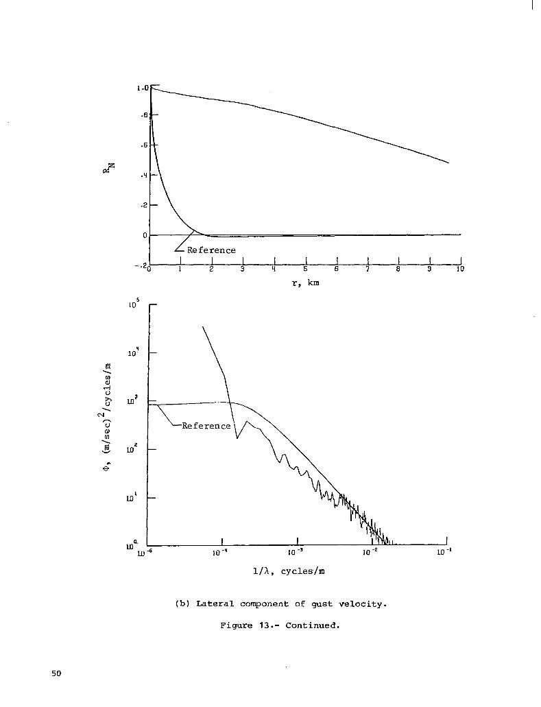
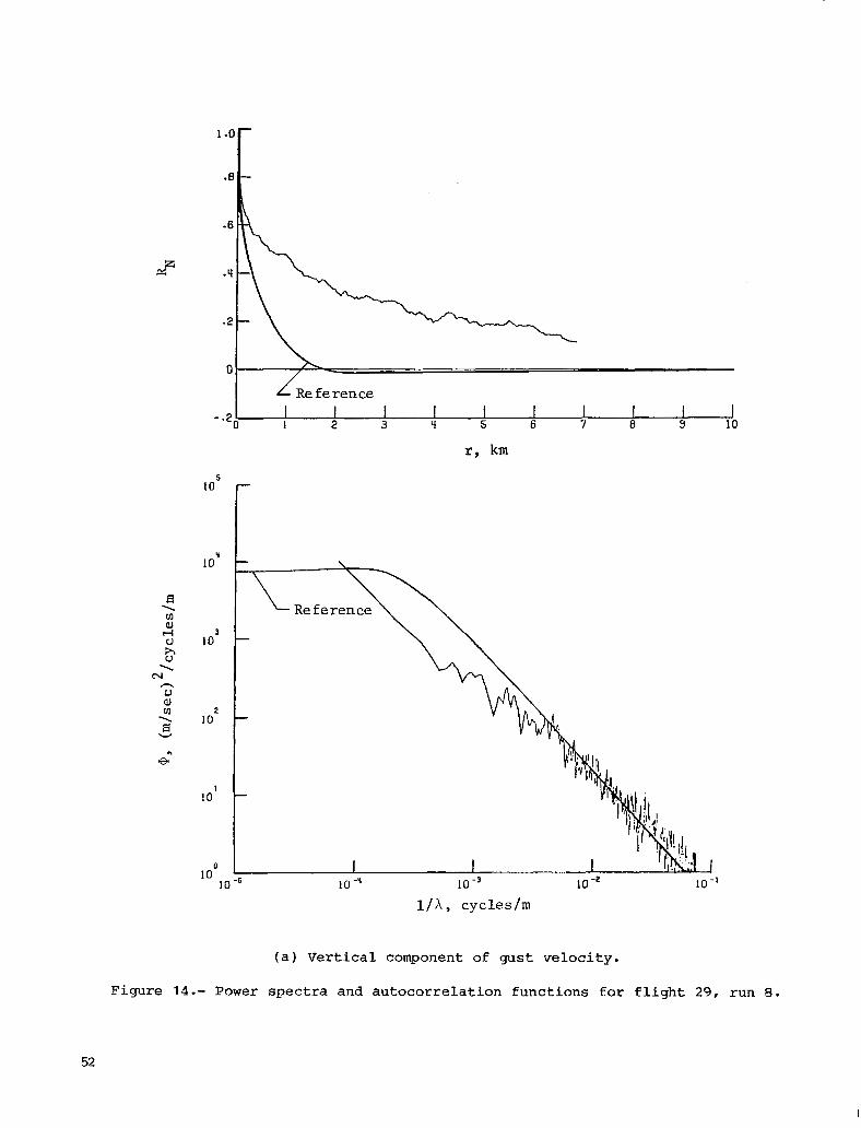
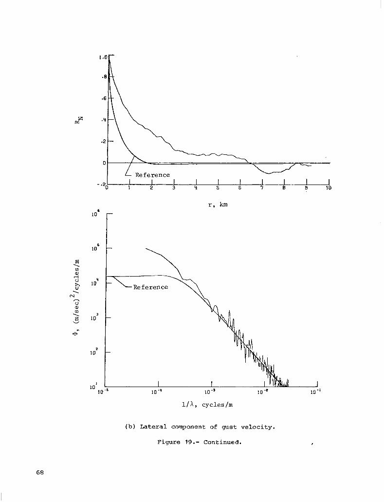
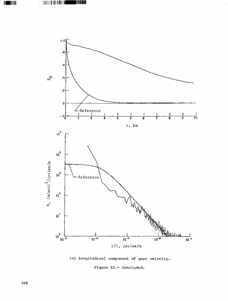
The au tocor re l a t ion and p o w e r spectra are p r e s e n t e d i n f i g u r e s 4 to 46. The order of presenta t ion fo l lows the o rder of t a b l e 11. The format is as fol lows: the normalized autocorrelat ion funct ion is presented a t the top of t h e f i g u r e , and t h e power spectrum is p r e s e n t e d i n t h e lower part of the f igure . In each case , for reference, a curve i s included for an a n a l y t i c a l a u t o c o r r e l a t i o n f u n c t i o n and a power spectrum defined by the Von K&m& expression. (See ref . 1 . ) Thus, €or the longi- t u d i n a l component,

and fo r t he t r ansve r se components,

2 L 1 + 8/3(1.339LO) 2 Q W ( Q ) = QJQ) = d - "

[ l + (1 .339LQ) 3 2 11/6

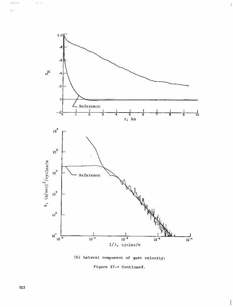
where 52 is the spa t ia l f requency 27c/h. A n i n t e g r a l s c a l e v a l u e L of 762 m (2500 f t ) , which is p resen t ly spec i f i ed i n t he des ign spec i f i ca t ion MIL-A-008861A ( s e e r e f . 1 2 ) fo r con t inuous t u rbu lence ana lys i s a t a l t i t udes above 762 m (2500 f t ) , was a r b i t r a r j l y s e l e c t e d f o r t h e r e f e r e n c e . It is t o be noted tha t L a s used i n t he Von Kirman expressions is a c t u a l l y t h e L va lue assoc ia ted wi th the longi tudina l component and is twice the L value of the transverse components. (See ref. 1, p. 1 3 . ) In each case, the reference curve w a s t r a n s l a t e d v e r t i c a l l y t o c a u s e t h e curve at short wavelengths to coincide with the measured data. Thus, the standard- deviation value of the re fe rence is d i f fe ren t for each ind iv idua l spec t rum. Each f i g u r e is i n t h r e e p a r t s t o p r e s e n t i n o r d e r t h e v e r t i c a l , l a t e r a l , and longi tudina l gus t -ve loc i ty da ta for a g iven f l igh t and run.

As s ta ted p rev ious ly , the p r inc ipa l purpose of this sampling program was t o investigate the long-wavelength air motion and measure its magnitude o r power r e l a - t i v e t o t h e s h o r t e r wavelength turbulence such as has been measured in several earlier sampling programs. Figures 4 t o 26 present tu rbulence da ta ca tegor ized a c c o r d i n g t o mountain-wave or orographic phenomena.

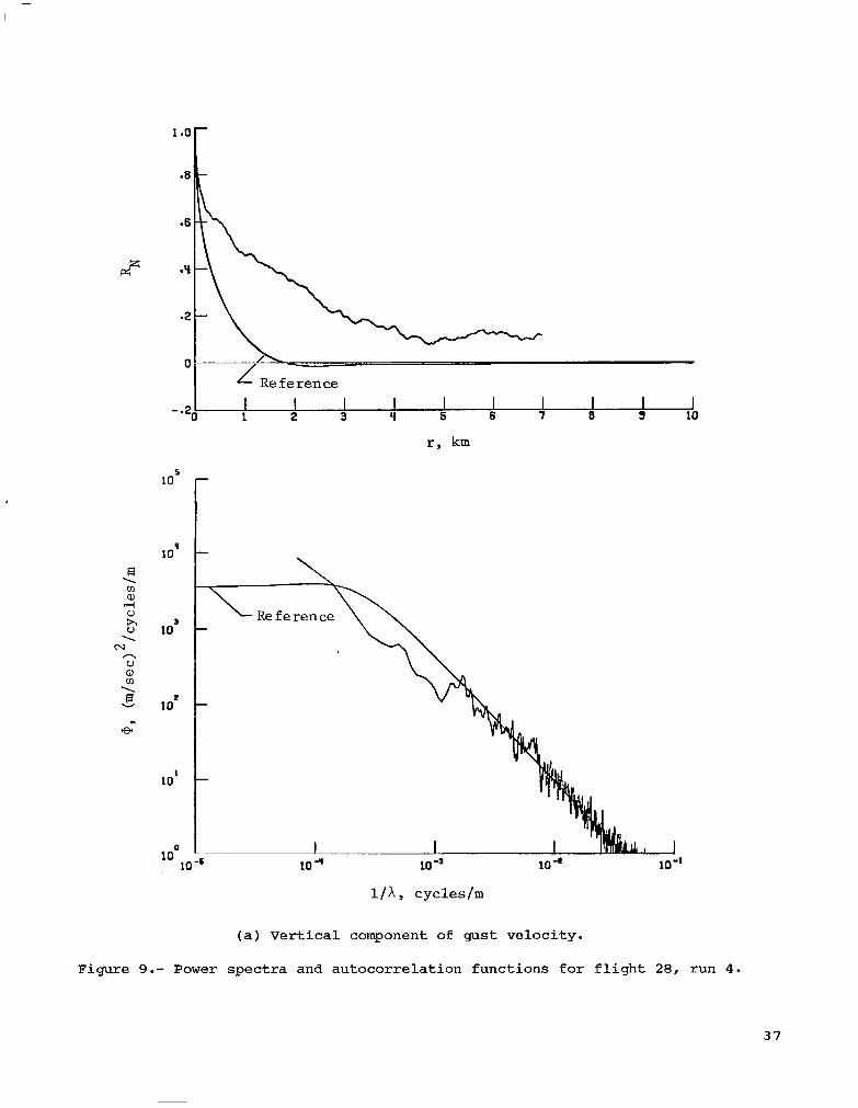
Figure 4 p re sen t s r e su l t s €o r a 680-sec run made a t an a l t i t u d e of about 1924 m ( 6 3 1 1 ft) over the Appalachian Mountains i n Western Virginia. (See table 11.) The number of s t a t i s t i c a l d e g r e e s of freedom is 27. I n f i g u r e 4 ( a), it can be seen t h a t a t the h igher f requency or shor te r wavelengths the var ia t ion of power density with f requency exhibi ts the -5/3 s lope cha rac t e r i s5 i c of most previous measurements and corresponds t o t h e y e d i c t i o n of t he Von K&nan expression. Below an inverse wavelength o f about 10- cycles/m, however , the data deviate s ignif icant ly from the r e f - erence Von Karrnan curve. In this region, the power is less than the re fe rence curve by roughly a f a c t o r of 2 f o r an inverse-wavelength interval of about 10-1 cycles/m,

. ,

6

and then the s lope o r power inc reases and the curve crosses over the reference curve for the longer wavelengths measured. This increase in power a t long wavelengths would be expected from observa t ion of the normalized autocorrelat ion funct ion which is presented a t t h e t o p p o r t i o n of t h e f i g u r e . The low po in t of t h i s a u t o c o r r e l a t i o n func t ion , which extends w e l l in to the nega t ive reg ion and occurs between a l a g d i s - t ance r of 6 km ( 19 685 f t ) t o 7 km (22 966 f t ) , is t y p i c a l of cases where atmo- spher ic tu rbulence is superimposed upon a s t r o n g wave. The au tocor re l a t ion func t ion fo r t he l ong i tud ina l components shown i n f i g u r e 4 ( c ) h a s a similar appearance because the run was made pe rpend icu la r t o t he waves. The minimum occurs a t one-half wavelength of t h e s t r o n g wave. This can be verified by examination of the t ime history which is p r e s e n t e d i n f i g u r e 4 7 ( a ) . (Some s i g n i f i c a n t t i m e h i s t o r i e s are discussed in the appendix and are p r e s e n t e d i n f i g s . 47 t o 49.) Here, it is s e e n t h a t t h e average t ransverse t i m e of 1 cyc le of the mountain wave is about 1 '/2 min, which pro- duces a one-half wavelength of approximately 6.3 km ( 2 0 669 f t ) when the average t rue a i r speed €or the run of 139.6 m/sec (458 f t / s e c ) is taken i n t o account. (-An under- s tanding of the appearance of autocorrelation functions associated with mountain waves c a n b e r e l a t e d t o t h e f a c t t h a t t h e a u t o c o r r e l a t i o n f u n c t i o n of a pure s ine wave is e s s e n t i a l l y a c o s i n e f u n c t i o n s t a r t i n g a t 1 a t r = 0 and going t o -1 a t r = h/2 , and then back t o 1 a t r = h.)

The reference curve on t h e ACF p l o t ( f i g . 4( c ) ) is f o r t h e Von Kgrmgn model wi th L = 762 m (2500 f t ) . As can be seen, the experimental ACF is un l ike t ha t €o r t he Von K&m& model because of t he predominance of t he wave e f f e c t . It is t o be noted that the one-half wavelength of 6.3 h ( = 2 0 600 f t ) i n d i c a t e d by t h e ACF should t r a n s l a t e t o a s t r o n g peak i n t h e power spectrum a t about 8 x lo-' cycles/m. How- ever, such a long wavelength is e s s e n t i a l l y below the r e so lu t ion capab i l i t y of t he p r e s e n t s p e c t r a l a n a l y s i s .

Severa l of the au tocorre la t ion func t ions ( those wi th very l o w s t a t i s t i c a l degrees of f reedom) exhibi t d iscont inui t ies . For example, f i gu re 15 (b ) has a d i s - c o n t i n u i t y a t r = 9 km ("29 500 f t ) . For r u n s processed with a l a r g e number of lags i n comparison t o t h e run length ( thus producing low s t a t i s t i c a l d e g r e e s of Ereedom), such d i s c o n t i n u i t i e s a r e o b s e r v a b l e a t a value of r equivalent to one-half the run length and r e s u l t from "noise" introduced by the mechanics of the data-reduct ion procedure.

Evidence of s t rong pe r iod ic con ten t is d i sce rnab le fo r a l l of t he mountain-wave f l i g h t s ( f i g s . 4 t o 26) from examination of the ACF i n a manner s i m i l a r t o t h a t p r e - viously discussed i n t h e example of f i g u r e s 4( a ) and 4( c ) . The s t r e n g t h of the wave, and the ve loc i ty component upon which it appears, is h ighly cor re la ted wi th the rela- t i v e a n g l e between t h e f l i g h t t r a c k and t h e o r i e n t a t i o n of t he r i dge t ops . The ver- t i c a l and longi tudina l gus t -ve loc i ty components exhib i t s t rong-wave conten t for t r acks pe rpend icu la r t o t he r i dge t ops . L i t t l e evidence of waves is p r e s e n t f o r t r a c k s p a r a l l e l t o t h e r i d g e € o r any component, s i n c e waves were not be ing in te r - cepted by the a i rp l ane .

In genera l , the PSD of f i g u r e s 4 t o 26 shows t h a t mountain-wave turbulence pro- duces greater long-wavelength power than the Von K&m& model. This is p a r t i c u l a r l y t r u e f o r t h e v e r t i c a l and long i tud ina l components when t h e f l i g h t p a t h is perpendicu- lar t o t h e r i d g e l i n e o r wave o r i en ta t ion . In f ac t , w i th t he poss ib l e excep t ion of t h e v e r t i c a l component shown i n f i c p r e 1 7 ( a ) , none of t h e mountain-wave da ta come v e r y c l o s e t o f i t t i n g t h e Von Kirman model a t low f requencies with a value of r e f e r - ence L of 762 m (2500 f t ) . Even f o r t h i s r u n , t h e knee of t h e PSD does not f i t very well . Since no s t rong wave is d iscernable on any component of t h i s r u n , t h e turbulence could have been generated by rough t e r r a i n o n l y ( r a t h e r t h a n by a mountain

7

range or ridge line) and, therefore, possibly should not be classed as "mountain-wave turbulence." Although the PSD of the longitudinal component for flight 34, run 5, fits the reference model quite well (fig. 19( c 1 1 , the ACF indicates a wave effect at N 2 of about 7 km ( =23 000 ft), which would result in power higher than the reference at an inverse wavelength somewhat lower than the lowest point o€ the PSD.

At the higher invers,e wavelengths, all of the data seem to have the -5/3 power drop-off of the Von Kirman model, with the possible exception of the vertical component of flight 39 (runs 3, 5, and 7 ) shown in figures 22(a), 23(a), and 24(a), respectively. The power drop-off for these runs seems to be slightly less steep; the cause for this is not known.

Another general observation is that for data which include wavelengths such as those presented herein, the standard deviation €or the horizontal components is nearly always greater than that for the vertical components. This is easily observed from inspection of table 11. Since long-scale variations are a part of the nature of the overall wind field which, of course, is horizontal in direction, the horizontal components will exhibit more overall power. This suggests that although the turbulence is isotropic at short wavelengtrhs, as has been traditionally assumed, isotropy does not hold for turbulence in the atmosphere at long wavelengths.

Figures 27 to 35 present the spectral data for wind shear including the cases where the jet stream is directly involved. From inspection of table II(b), it is seen that the variability in standard deviation was small. The intensity of the vertical component was always lower than that for the horizontal components and did not exceed 0.9 m/sec (2.9 ft/sec), whereas the intensity of the horizontal components was somewhat more variable from sample to sample.

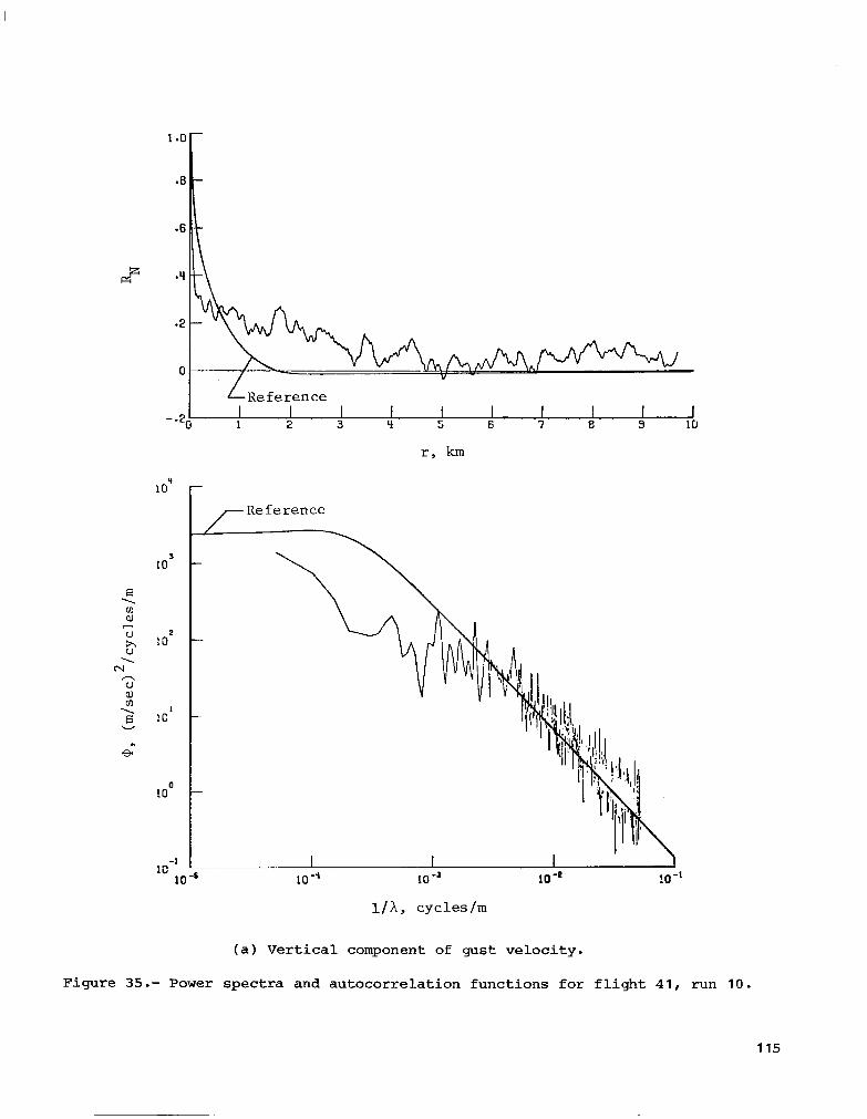
In contrast to the mountain-wave turbulence, a number of the vertical-component cases contain less power in the long-wavelength region than the reference curve for the Von Karman model. (For example, see fig. 28(a).) In every case, however, the horizontal components contain much greater power in the long-wavelength region than the reference curve. Examination of the ACF for the cases of wind shear and/or jet- stream effects indicates that the time histories are dominated by low-frequency drift or trendlike effects, which would show up in the PSD at frequencies near zero. This is evidenced in the ACF by a curve with low slope. The spectra all appear to follow the -5/3 slope of the Von K&m& model in the shorter wavelength region.

, .

After studying the ACF of flight 38 (figs. 31(a) and 32(a)), it is apparent that a strong wave is present on the vertical component. The indication is, therefore, that the turbulence for this flight was predominately "mountain wave" in nature, rather than the "short-wave-trough movement" suggested in reference 9.

Figures 36 to 46 present data that are considered to represent special meteorological conditions that cannot be considered representative of the other categories. On flight 8 (fig. 361 , turbulence associated with convection was sampled at an altitude of 460 m (1500 ft). This case was presented previously in reference 6 and is shown to €it the Von K&m& model remarkably well when a value of L of 305 m ( 1 0 0 0 ft) is used for the vertical component. Somewhat larger values of L are required to fit the horizontal components: about 600 m (=2000 ft) for the lateral component and 1200 m (~4000 ft) for the longitudinal component. Sample time histories are shown for this low-altitude convective turbulence in reference 6. Although the time histories for all three components are very similar in appearance, the ACF and PSD indicate that even low-altitude convective turbulence is not isotropic in the long-wavelength region. The rapid drop in the power spectra at the

8

shortest wavelength end (i.e., below the -5/3 reference curve) for figure 36 is a result of an experiment employing a digital antialiasing filter. It was determined that aliasing was not a problem, and use of the filter was, therefore, discontinued for all other data.

Flight 32, run 4, was originally presented as a high-altitude wind-shear case in reference 6 . (See fig. 39.) The meteorological and other aspects of this flight have also been reported in detail in reference 7. The meteorological analyses indi- cated that the turbulence encountered on this flight was triggered by wind shear; however, some of the runs appeared to contain orographic effects, and the intensity was generally greater for those than for the remaining cases for wind shear and/or jet-stream effects. For that reason, flight 32 was grouped with the "special cases" in the present paper. The time history of run 4, which is shown in reference 6 (also see the appendix of the present paper), is believed to be typical of high-altitude wind shear and shows no orographic or wave effects. The horizontal components are illustrative of the cause of the high power near zero frequency on the PSD curves, which is typical of wind-shear turbulence. As previouslx sh,own in reference 6 , the vertical component for run 4 (fig. 39(a)) fits the Von Karman model quite well, indicating an L value of about 305 m (1000 ft). The horizontal components have, c?n- siderable more power at the long wavelengths and do not conform to the Von Karman model, as is evident from the ACF curves.

Another special case which appears to conform to the Von Karman model quite . .

well, as far as the vertical component is concerned, is flight 4 2 , run 6 . (See fig. 44(a).) Flight 42 was conducted in mixed conditions associated with low- altitude thermal convective action and sea-breeze convergence. (See ref. 9.) Run 6 was a low-altitude run exhibiting moderate and greater turbulence intensity. The horizontal components €or these data also contain much more power at the long wavelengths than the reference curve, with the ACF curves indicating that the power is at a very low frequency.

Data presented herein indicate that the Von Karman model is good at short wavelengths, but significant differences can be present at long wavelengths depending on the atmospheric situation. Some recent studies related to alternate modeling of atmospheric turbulence are reported in references 13 to 17. In general, the alternate models take into account the fact that, for power spectral representation to long wavelengths such as the measurements described herein, "turbule2ce': by the con- ventional definition may be described by a curve composed of a Von Karman component which is adequate at short wavelengths; but an additional term must be included to account €or the additional power at the longer wavelengths because of the special long-wave content.

. .

The time histories presented for figures 47 to 49 are discussed in the appendix for cases of wave motion to point out significant characteristics that cannot be easily observed from power spectra.

CONCLUDING REMARKS

Measurements of three components of clear-air atmospheric turbulence have been made with an airplane incorporating a special instrumentation system to provide accurate data resolution to wavelengths of approximately 12 500 m ( 4 0 000 ft). Flight samplings covered an altitude range from 500 to 14 000 m (1500 to 46 500 ft) in various meteorological conditions. Individual autocorrelation functions and power spectra have been presented for the three turbulence components from 43 data runs.

The majority of the data are from mountain-wave and jet-stream encounters. The use of power spectral-density design techniques for the response of airplanes to atmospheric turbulence requires a mathematical model describing atmospheric turbulence in power spectral form.

The present data support previous data confirming that the Von K&m& model is a realistic representation of atmospheric turbulence at wavelengths shorter than about 1000 m (3281 ft), and it is thus usable for designing subsonic airplanes whose pri- mary response modes fall below this wavelength. (Past successful airplane design, of course, bears this out.) It should be noted that experimental limitations in this measurement program (primarily those of record or sample length) prevent the reliable resolution of integral scale values L greater than about 1800 m (~6000 ft) since location of the "knee" of the Von K&r&n model for such high L values is at a longer wavelength than data can be reliably processed. The present data, however, show that although the design value of L of 762 m (2500 ft) specified in MIL-A-O08861A, when tied to the appropriate intensity level a, results in proper subsonic design loads, it does not realistically represent what takes place in the atmosphere at wavelengths greater than 1000 m (=3000 ft).

The limitations of the Von K&&n turbulence model at wavelengths greater than 1000 m ( 4 0 0 0 ft) are of particular significance for many situations involving wind- shear and mountain-wave conditions. The difficulty in specifying an appropriate value of L makes its use difficult for other types of turbulence as well.

Models which appear to be capable of realistically describing atmospheric turbulence behavior throughout the total range of wavelengths are described in NASA CR-145247 and CR-2913. It appears that an analytical model consisting of the sum of a "slow component" as a function of tfme,, plus an amplitude-modulating function of time multiplied by a so-called "Von Karman component," would be required to describe many of the power spectra presented in this report. However, the determination of statistical parameters to insert into such a model to represent adequately an overall airplane turbulence experience would seem to be a formidable task.

A practical approach, and possibly just as accurate, for overall design-loads prediction in a wavelength region greater than about 1000 m ( 4 0 0 0 ft) would be to use the Von K&m& equation with a fixed and conservatively larger value of L. The model used in this fashion would be recognized as being approximate only, and it would also require additional research to determine appropriate combinations of L and a.

Langley Research Center National Aeronautics and Space Administration Hampton, VA 23665 March 3 , 1982

10

APPENDIX

SELECTED TIME HISTORIES

Examples of wave phenomena can be seen in the time histories of figure 47. In figure 47(a), the three components of gust velocity are shown for a 14-min data run of a track diagonal to the ridges at an altitude of 1924 m (6311 ft) in what was classified in reference 13 as an Appalachian mountain-wave situation. The low- frequency oscillations prominent on the vertical and longitudinal time histories are characteristic of mountain waves. It would appear that the predominant wavelength is about 13 km (=8 miles, 1.5 min). The turbulence intensity is quite variable, but it is interesting to note that the intensity is always high for all components on the positive slope of the wave. Figure 47(b) is a 9-min portion of a run on the same flight parallel to the ridges. Again, a significant wave pattern is obvious on the vertical and longitudinal components. Gust-velocity time histories from other runs of the same flight are shown in figures 47(c), 47(d), and 47(e).

Time histories for a 5-min run in a mountain-wave situation at about 14 0 0 0 m ( x46 000 ft) near the Sierras is presented in figure 48. In this case, the turbulence intensity is low, but wave motion is very predominant with a peak-to-peak longitudinal gust velocity of about 19 m/sec ( 6 2 ft/sec) over a 1-min interval. Oscillations in the vertical gust velocity were of lower amplitude and at a higher frequency, about 1.5 cycles/min.

Some other interesting wave phenomena are shown in figure 49 for a flight at an altitude of about 10 700 m (=35 0 0 0 ft) that was categorized in reference 9 as being predominantly influenced by jet-stream effects, but in the presence of mountain waves. The time histories clearly show the very long wavelength (low-frequency) effects of shear on the horizontal components (especially noticeable in fig. 49(d)) with the shorter waves present on all components. The turbulence intensity ranged from light to very light.

\

11

REFERENCES

1. Houbolt, John C.; S t e ine r , Roy; and P r a t t , K e r m i t G.: Dynamic Response of A i r - p l a n e s t o Atmospheric Turbulence Including Flight Data on Input and Response. NASA TR R-199, 1964.

2. Murrow, Harold N.; and Rhyne, Richard H.: The MAT P r o j e c t - Atmospheric Turbu- lence Measurements With Emphasis on Long Wavelengths. Proceedings of the Sixth Conference on Aerospace and Aeronautical Meteorology of the American Meteoro- log ica l Soc ie ty , Nov. 1974, pp. 313-316.

4. Keisler, Samuel R.; and Rhyne, Richard H.: An Assessment of Prewhitening i n Est imat ing Power Spectra of Atmospheric Turbulence a t Long Wavelengths. NASA T N D-8288, 1976.

5. Rhyne, Richard H.: F l i g h t Assessment of an Atmospheric Turbulence Measurement System with Emphasis on Long Wavelengths. NASA TN D-8315, 1976.

6. Rhyne, Richard H.; Murrow, Harold N.; and Sidwell, Kenneth: Atmospheric Turbu- lence Power Spec t r a l Measurements t o Long Wavelengths fo r Seve ra l Meteoro- log ica l Condi t ions . Ai rcraf t Safe ty and Operating Problems, NASA SP-416, 1976, pp. 271-286.

7. Waco, David E.: Mesoscale Wind and Temperature Fields Related t o a n Occurrence of Moderate Turbulence Measured i n t h e S t r a t o s p h e r e Above Death Valley. Mon. Weather Rev., vol . 106, no. 6, June 1978, pp. 850-858.

8. Davis, Richard E.; Champine, Robert A . ; and Ehernberger, L. J.: Meteorological and Operation Aspects of 46 Clear Air Turbulence Sampling Missions With an Instrumented B-57B A i r c r a f t , Volume I - Program Summary. NASA TM-80044, 1979.

9. Waco, David E.: Meteorological and operat ional Aspects of 46 Clear Air Turbu- lence Sampling Missions With an Instrumented B-57B A i r c r a f t , Volume I1 (Appendix C ) - Turbulence Missions. NASA TM-80045, 1979.

10. Meissner, Charles W., Jr.: A F l igh t Ins t rumenta t ion System for Acquis i t ion of Atmospheric Turbulence Data. NASA TN D-8314, 1976.

11. Otnes, Robert K.; and Enochson, Loren: D i g i t a l T ime Ser ies Analys is . John Wiley & Sons, Inc., c.1972.

1 2 - Airplane Strength and R ig id i ty - Fl igh t Loads. M i l . Specif . M I L - A - O O ~ ~ ~ I A (USAF), Mar. 31, 1971.

13. Sidwell , Kenneth: A Mathematical Study of a Random Process Proposed as a n Atmo- spheric Turbulence Model. NASA CR-145200, 1977.

14. Sidwell, Kenneth: A Qua l i t a t ive Assessment of a Random Process Proposed as a n Atmospheric Turbulence Model. NASA CR-145247, 1977.

12

I -

15. Mark, William D.: Characterization of Nongaussian Atmospheric Turbulence for Prediction of Aircraft Response Statistics. NASA CR-2913, 1977.

16. Mark, William D.; and Fischer, Raymond W.: Statistics of Some Atmospheric Turbu- lence Records Relevant to Aircraft Response Calculations. NASA CR-3464, 1981.

17. Mark, William D.: Characterization, Parameter Estimation, and Aircraft Response Statistics of Atmospheric Turbulence. NASA CR-3463, 1981.

13

TABLE I.- PREDOMINANT METEOROLOGICAL CONDITION AND GENERAL

GEOGRAPHICAL LOCATION FOR FLIGHT DATA RUNS PRESENTED

Flight

2 0

2 8

2 9

3 0

3 3

3 4

3 9

2 4

27

3 8

41

Number of data runs presented

Predominant meteorological condition

( a )

Mountain-wave and/or orographic effects ~~

Appalachian Mountain wave

Low-altitude wind shear and orographic effects

Mountain-wave and low-level orographic effects: rotor zone

Mountain wave

Low-level orographic effects

Low-level mountain wave

Mountain wave and intense upper f ront

Wind-shear and/or jet-stream effects

Strong vertical and horizontal wind shears below jet stream

Low-level j e t stream with ver t ical wind shear below

Short-wave-trough movement

Fast-moving wave trough with ver t ical and horizontal wind shears

Flight locatio!

( a )

VA

CA

CA

CA

CA

CA

CA

VA

VA

CA

CA

~~ ~ ~~

Special cases

8 VA Low-altitude convection 1

32 4 Complex orographic effects; ver t ical wind shear; j e t stream (Death Valley f l i gh t )

CA

42 CA Low-altitude convection and 6 sea-breeze convergence

aInformation for th i s column is taken from reference 8.

14

I --

TABLE 11.- TEST CONDITIONS AND MEASURED STATISTICAL DATA

Figure

4

5

6

7

8

-~

9

10

1 1

I I

( a ) Turbulence data according t o mountain-wave and/or orographic effects

Mean Data-run length Data run

UU UV OW S t a t i s t i c a l dof a l t i t u d e ~ - for p o w e r spectra

m m/sec Time, Distance, m/sec m/sec ( f t ) km ( f t ) sec ( f t/sec) ( f t/sec) ( f t/sec) ( a )

Fl ight 20 on December 3, 1974; 16:46 to 18:59 GMT

1

2

3

4

5

1 924 (6 311)

1 891 (6 205)

1 882 (6 173)

1 899 (6 231)

1 920 (6 298)

94.9 (311 352

74.6 (244 751

93.9 (308 071

55.6 (182 415

44 .O (144 357

680 - 0 0

549.95

686.00

4 19 .OO

333 .oo

27

21

27

16

13

2 .22 (7.28)

1.44 (4.74)

1.87 (6.13)

1.65 (5 -42 )

1.59 (5.22)

Flight 28 on February 14, 1975; 13:22 t o 15:31 GMT

1 537 (5 042)

1 897 (6 223)

1 157 (3 796)

aSee reference 11.

88 -0 (288 714)

68 -6 (225 066)

124.8 (409 449)

646 .OO

496 .OO

912 .OO

25

19

36

1.50 (4.92 )

1.41 (4 -62 )

1.92 (6.29)

Fl ight 29 on February 20, 1975; 19:07 to 21:38 m T

98 -2 (322 178)

190.8 (625 984)

106.3 (348 753 )

537.00

10 18 -00

796.00

1.98 (6.48)

1.44 (4.73)

2.34 (7.68)

3.59 (11.77)

3 -60 (11.80)

3 -07 (10.08)

2 .61 (8.56)

4.17 (13.67)

I I

3.79 (12 .42

2.45 (8.05)

3 .2 1 (10 -53)

2 -24 (7.35)

2.90 (9.50)

2 -04 (6.68)

2.19 (7.19)

3.94 (12 -94)

21

40

31

~ 1.10 ' (3.61)

1.07 (3.51)

1.73 (5.66)

5.20 (17.07)

1.92 (6.3 1)

6 -43 (2 1.09)

3.51 (11.50)

2 -08 (6.82

3 -15 ( 10 -33 )

15

TABLE 11.- Continued

( a ) Concluded

1 Figure 1 =un Data a l t i t ude

Distance, km (ft)

length S t a t i s t i c a l dof

for power spectra

( a ) rn/sec m/sec rn/sec Time,

sec

Flight 30 on March 7, 1975; 21:42 t o 00:47 GMT

~ ~~

=-T (8.40) -

1.03 (3 .38)

4.30 (14.11)

14 114 (46 306)

91 .oo

754.40

4

29

0.68 (2 -23 ) 0.68 (2 -23 ) (59 383)

148.7 (487 861)

14 265 (46 800)

1.34 (4.41) 1.34

(4.41) I

I Flight 33 on March 28, 1975; 18:47 t o 2 0 ~ 4 8 GMT ~. .

89 -00 (291 995)

3.90 3.45 1.27 23 592 .OO (12.80) (11.33) (4.16)

~~~ ~

2 638 (8 656)

I Flight 34 on April 4, 1975; 18:50 t o 21:30 GMT

(14 245) ( l a 415) 342 55.6 I 306.15

332 .OO

485.95

2 .05 (6.71)

2.34 (7.68)

3 -82 (12 -52 )

3.78 (12 .39)

4 -84 (15.87)

5.51 (18.09)

2.64 (8.66)

2.80 (9.19)

3 -58 (11.73)

12

13

19

18 3 4 342 55.6 306.15 (14 245) ( l a 415)

19 5 3 874 59.7 332 .OO 3 874 59.7 1 (12 709) (195 866) (12 709) (195 866)

20 7 3 892 88.5 485.95 (12 770) (290 354) 3 892 88.5 1 (12 770) (290 354)

Flight 39 on May 20, 1975; 18:13 t o 20:26 GMT " .~

2 .38 (7.80)

2 -48 (8.15)

4.04 (13.25)

3 -19 (10.45)

7.0 1 (23 .OO)

4.63 (15.19)

-

338.50

2 48 -00

456 .OO

406.95

561 .OO

100.05

13

10

18

16

22

4

1.06 (3 .48)

0.96 (3 .16)

1.08 (3.54)

1 . 12 (3.67)

1.42 (4.65)

2.08 (6.83)

60 -6 (198 819)

45.4 (148 950)

86 -0 (282 152)

77.7 (254 92 1)

108.9 (357 283 )

19.2 (62 992 )

4.81 (15.79)

4.70 (15.43)

4.16 (13 -65)

6.65 (2 1.83)

3 .02 (9.92

3.65 (11.98)

21

22

23

24

25

26

2

3

5

7

9

10

3 210 (10 532

4 127 (13 539:

4 135 (13 566)

4 180 (13 715)

4 208 :13 805)

4 157 :13 638)

aSee reference 11.

16

I -

TABLE 11.- Continued

(b) Turbulence data according t o wind-shear and/or jet-stream effects

alt i tude Mean I Data-run length I Statist ical dof QU

Data run Figure

27

28

29

for power spectra m

(ft/sec) (ft/sec) (a) sec km ( f t ) (f t) m/sec m/sec Time, Distance,

Flight 24 on December 17, 1974; 16:12 to 18:04 GMT

m/sec ( f t/sec)

I 18

21

b28

c14

5 903 (19 366)

5 891 (19 328)

5 904

(19 369)

457.00

535.00

b715.00

c353.00

0.46 (1 -50)

0.48 (1.57)

0.71 (2.32)

2.31 2.35 (7.95) (7.70)

3.04 (12.98) (9.96) 3.96

83.3 (273 294)

98.7 (323 819)

b131.9 (432 743)

C 65.1 (213 583)

3.23 (10.59)

3.01 (9.89)

anuary 30, 1975; 15:48 t o 18:07 GMT F l i g h t 27 on J I I 'I I I I I I

30 I 13 2.23 1.03 0 -58 1 1 280 -00 51 -8 10 605 (34 793) (7.30) (3.39) (1.90) (169 948)

Flight 38 on April 24, 1975; 22:lO to 00:54 GMT

31

32

33

337.00

694.00

780.95

13

27

31

0.75 (2.47)

0.67 (2.20)

0 -89 (2.92)

2.83 (9.27)

3.10 (10.18)

5.18 (17.00)

10 637 (34 898)

10 705 (35 120)

10 649 (34 938)

63.58 (208 596)

132.4 (434 383)

145.7 (478 018)

2.41 (7.92)

1.70 (5.58)

4.78 (15.68)

L

Flight 41 on May 21, 1975; 21:50 to 00:34 GMT

7 368 (24 172)

184.00 1.55 1.49 0 -72 7 (2.37) (5.09) (4.89)

247.05 2.32 2.16 0.79 10 (2.60) (7.61) (7.09)

7 411 (24 314) (153 543)

%ee reference 1 I. bValues for w data only. %alues for v and u data.

17

TABLE 11.- Concluded

(c) Special meteorological cases

Data-run length S t a t i s t i c a l dof

7 Distance, Time, for power spectra

m/sec m/sec m/sec km ( f t ) ( a )

Fl ight 8 on June 19, 1974; 18:09 t o 19:32 GMT

36 45 1.15 1.18 1.34 1146.35 147.6 460 2 (1 509) (3 -78) (3 -86) (4.41) (484 252 )

Flight 32 on March 26, 1975; 19:46 t o 22:19 6 I T

3 1

38

39

40

41

42

43

44

45

46

12 989 (42 615)

13 056 (42 835)

12 984 (42 600)

13 070 (42 879)

115.8 (3 79 92 1)

65.1 (2 13 583)

136.8 (448 819)

130.6 (428 478)

634 .OO

367.00

728.80

699 .OO

25

14

28

27 I 2 .24 (7.34)

2 .04 (6.68)

2.45 (8.05)

1.52 (4.99)

4 420 [14 500)

4 420 :14 500)

4 420 :14 500)

1 676 (5 500)

3 200 10 500)

3 200 10 500)

Flight 42 on June 13, 1975; 18:ll to 20:17 GMT

84.8 (278 215)

102 .6 (336 614)

57.7 (189 304)

79 .O (259 186)

54 .O :177 165)

66.5 12 18 176)

423.95

512 .95

2 90.85

544.80

272 .oo

334.85

17

20

1 1

21

1 1

13

1.91 (6.28)

1.79 (5.86)

1.41 (4.63)

2 .05 (6.74)

1.76 (5.76)

2 .39 (7.83)

8.41 (27.60)

4.72 (15.50)

7 -32 (2 4.02

8.75 (28.72)

2 .2 1 (7.25)

2 .2 7 (7.46)

2.90 (9.53 )

2 .69 (8.81

2 -84 (9.33 )

3 .15 '10.34)

3.33 (10.92

3 .17 ( 10.40)

4.47 (14.67)

5.70 (18.69)

2 .80 (9.20)

2 .07 (6.80)

2 .25 (7.39)

4.2 6 (13 -99)

1.56 (5.12)

2 .14 (7.01) "

aSee reference 11.

18

Figure 1.- Photograph of t he sampling airplane.

r C

@: i

L. ,Roanoke i I

i A' Scale

0 28 mi

0 45 km -

S

\' I @Washington, D.C.

++Predominant r idge areas

@ Base of operat ion ....

0 Area c i t i e s

@ Chesapeake Bay

Elevat ion above 850 m (280Q f t)

...

Shenandoah National Park

---Blue Ridge Parkway (-1 """""-

Figure 2.- Location of f l i g h t t r a c k s for f l i g h t s i n the Eastern United States.

0 Fresno

0

45 km

0 Pomona : P 3

"+. ._.. Predominant ridge areas '3,

A Elevation 850 m (2800 f t ) t o 2500 m (8200 ft) A Elevation above 2500 m (8200 f t ) + Elevation 86 m (282 f t ) below sea l e v e l @ Base of operation

Area c i t i e s

% %

Kings Canyon National Park Sequoia National Park

@ Death Valley National Monument

Figure 3.- Location of f l i g h t t r a c k s for f l i g h t s i n t h e Western United States.

2 1

- . 2 -

- . Y - --60 I I I I I I I 1 2 3 9 5 6 7 8 9 10

I I I I I I I 1 2 3 9 5 6 7 8 9 10

11 X, cycleslm

(a) Vertical component of gust velocity.

Figure 4.- Power spectra and autocorrelation functions for € l i g h t 20, run 1.

22

.e

.6

.Y

.2

0

- .2

5 10

1 oq

103

loz

10’

LReference I I I I I I I 1

1 2 3 Y 5 6 7 8 9 10

r, km

10 -q IO -’ 10 -2 10 -‘ 11 A , cycleslm

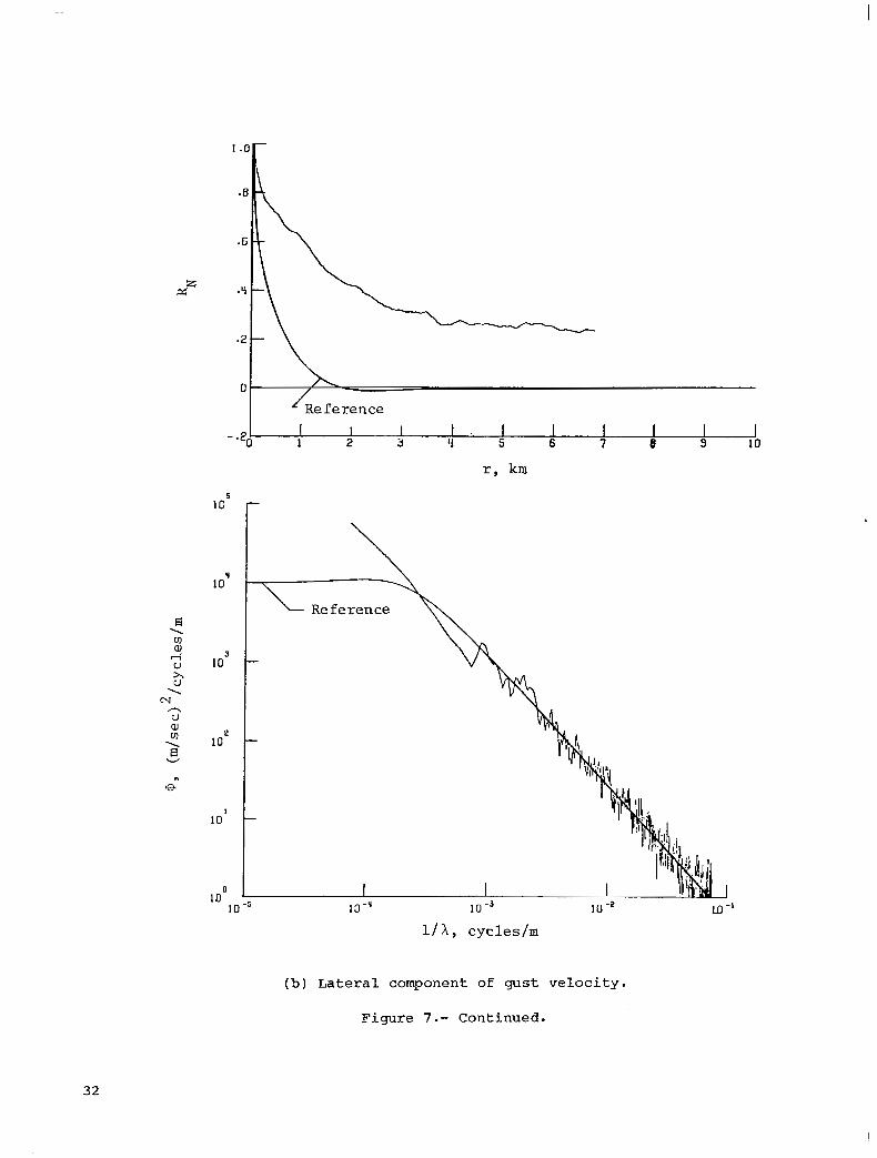
(b) Lateral component of gust ve loc i ty .

Figure 4.- Continued.

23

- .Y I I I I t I I I 0 1 2 3 Y 5 6 7 8 9 10

-1- -_I

r, km 5

.- 10 -q 10 - 3 10 -2

1 /X, cycles/m

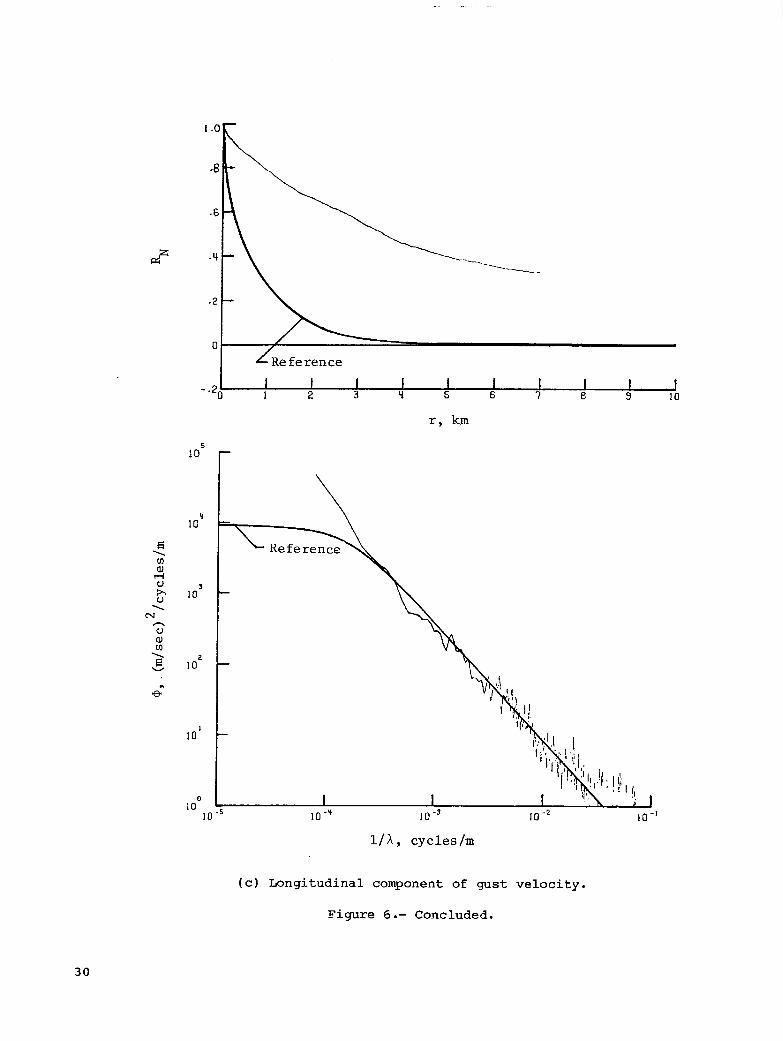
( c ) Longitudinal component of gust ve loc i ty .

Figure 4 .- Concluded.

2 4

r y km

11A cyc les lm


Figure 5.- Power spectra and autocorrelation functions for flight 20, run 2.

25

U '

LRe fe rence -

- .20 I I I I I i I 1 I I 1 2 3 Lf 5 6 7 '8 9 10

r , km

10'

IO'

IO'

1 o2

IO'

\

IO 10 -5

l/X, cycles/m 10 - 2

(b) L a t e r a l component of gus t ve loc i ty .

Figure 5 .- Continued.

2 6

I I1 I I I1 I

I --

- .2 -

-.Yo I I I 1 I I I I I I 1 2 3 5 6 7 8 3 10

r, km

lo’ r IO1

1 / X , cycleslm

( c ) Longitudinal component of gus t velocity.


2 7

r, krn

l/X, cycleslm



2 8

I .o

.6

.4 .2 *8!B -

0 L' Re fe rence

- ""

- '20 I I I I I I I I I I 2 3 9 5 6 7 8 9 10 - -21, I I 2 I 3 I 9 I 5 I 6 I 7 I 8 9 I 10 I

5 ID

Y 10

3 10

2 10

IO'

r, km - Reference

1/X, cycleslm



29

l/X, cycleslm

( c ) Longitudinal component of gus t ve loc i ty .


30

r, km

l / X , cycleslm


Figure 7.- Power spectra and autocorrelation functions €or flight 20, run 4.

3 1

1 .I

. f

.E

.Y

.Z

0

- .2

5 10

loq

IO'

lo2

10'

I I 1 2 3 '1 5 & 7 I 8 3 10 i

r , km

\ Reference

11 A, cyclesln;

(b ) L a t e r a l component o f gust ve loc i ty .


32

1 .I

.E

.6

.Y

.2

0

- -2

10’

1 oq

1 o3

lo2

10’

LO0 10

L Reference

I I 1 . I I I I I I I 1

- - ~. 2 3 Y 5 6 7 8 3 10

r, km

10” 1 0 - ~ 10 10 - I

l l h , cycleslm

( c ) Longitudinal component of gust v e l o c i t y .


33

Y 10

10'

lo2

lo1

0 10

Y 10 -

Ref e ren ce

10' -

lo2 -

lo1 -

0 10 -

1c-I _1 I I 1 I 10 -s IO -* 10" 10 - I 10 -1

I f X, cycles/m

1c-I _1 I I 1 I 10 -s IO -* 10" 10 - I 10 -1

I f X, cycles/m

(a) Vert ical component of gust velocity.

Figure 8.- Power spectra and autocorrelation functions €or f l i gh t 20, run 9.

34

1 .a

.6

.2

0

- .2,

10'

lo*

I o.~

1 o2

10'

loo 10

I I I I I I 1 I I J 1 it 9 Y 5 6 I 8 9 10 I I I I I I 1 I I J 1 it 9 Y 5 6 I 8 9 10

r , km

n Re f e ren ce

1

10 -% 10 -3 10 -2

l / X , cycles/m

10 -'



35

- -20 1 I 1 I I I I I I 1 2 3 Y 5 6 7 8 9 10

10'

10%

10'

lo2

1 o1

I O0 10

r, km

-

10 -y 10 -3 10 - 2 10 -I 10 -y 10 -3 10 - 2 10 -I

1/X, cycleslm

( c ) L o n g i t u d i n a l c o m p o n e n t of g u s t v e l o c i t y .

F i g u r e 8.- Conc luded .

3 6

l/X, cycleslm



37

1 .c

.a

-6

2 4

.2

0

- .2[

IO'

loq

IO'

lo2

IO'

LO0 IO

l R e f e rence I I I 1 I 1 1 I I 1 1 2 3 Y 5 6 7 8 3 10

r, km

n Re f e rence "\ h

I I I L , 1 10 -' 10 -3 10 -L to"

l / X , cycleslm

(b) Lateral component of gus t ve loc i ty .


38

II -

r, km

10'

10'

IO'

lo2

10'

IO0 u

T Reference

I I IO -* 10 4 10 -L 10 -'

1/X, cycles/m

(c) Longitudinal component of gust velocity.


39

- .20 I I I 1 I I I 1 I 1 2 3 '1 5 6 - 7 - ~~ 8 9 10

I O Y

lo3

lo2

10'

loo

r, km

-

1/X, cycles/m


Figure 10.- Power spectra and autocorrelation functions for flight 28 , run 6.

40

- .20 I I I I I I I I I I 1

I 2 3 9 5 6 7 8 3 10

. . .. -

* 0 5

loy

10 3

loe

l o *

loo IC

r y km

-

l / X , cycles/m

(b) Lateral component of gust veloc i ty .


4 1

1 .c

.E

.6

2 .Lt

.2

0

- .2,

lo5

loy

10'

lo2

10'

loo 10

l R e f e rence

I I 1 I I I I I I 1 2 3 Y 5 6 7 6 3 10

r, km

l R e f e r e n c e

I I 1 I I I I I I 1 2 3 Y 5 6 7 6 3 10

r, km

\

10 -y 10 -a 10 -I

1/X, cycleslm

10"

(c) Longitudinal component of gust ve loc i ty .


42

1 .a

.8

.6

.2

n

- .2,

\ rn a,

B

4 u h U

N \

n

a, u rn \ fi

W

e

i0 5

10%

2 10

1 10

IO0 1

r, km

i0 5

10%

2 10

1 10

IO0 10 -5 10 -q 10 -' 10 -1

1 / A , cycles/m

( a ) V e r t i c a l component of gus t ve loc i ty .

Figure 11.- Power spectra and au tocorre la t ion func t ions for f l i g h t 28, run 8 .

43

I I I I I J 1 2 3 Lt 5 6 7 8 9 10

1 ut

10‘

1 oq

10’

l o p

10’ 10

r, km

-

(b) Late ra l component of gust veloc i ty .


44

L Reference

- .20 I I I I I I I 1 2 3 9 5 6 7 8

l o 6

1 m aJ 4

a

u lo4

r, km

\

1 / A , cycleslm

(c ) L o n g i t u d i n a l c o m p o n e n t of gust v e l o c i t y .

F i g u r e 1 1 .- Conc luded .

45

- I I I I I I I I 1 2 3 Y 5 6 7 6 3 10

Figure 12.- Power spectra and autocorrelation functions for f l i gh t 29, run 6.

46

I O L 1

r, km

10 -q 10 -3 10 -?

l/X, cycleslm

(b) Lateral component of gust v e l o c i t y .


47

0

- .iIO I J 1 2 'k 3 Y 5 6 7 8 IO

-

r, km

1 o6

IOS

I O 5

I 0'

2 10

I 10

IO

* Reference

(c) Longitudinal component OP gust ve loc i ty .

Figure 12.- Concluded.

48

1 .(

.t

.E

.Y

-2

C

- .2

l o 5 r

L Reference " I I I I 1 1 I

1 2 - -~ 3 9 5 6 7 8 3 10

r, km

lo5 -

9 10 -

3 10 -

I O ' -

I 10 -1 10 -1


49

I I I I I I I I I 1 1 2 3 Y 5 6 7 8 9 10

r, km

-.20 I I I I I I I I I 1 1 2 3 Y 5 6 7 8 9 10

r, km

- \

1 / A , cycles/m

(b) Late ra l component of gust ve loc i ty .


50

Reference I "2 "- . I I I I I I

@ I 2 3 5 6 I 8 Y io

r, km S

10

Y 10

3 10

2 10

I D '

0 10

10



51

I I I 1 7 8 3 10

r, km

10’

IO’(

1 o3

2 10

I 10

lo* 10

l/X, cycles/m


Figure 14.- Power spectra and autocorrelation functions €or €light 29, run 8.

52

I .c

.a

-6

.Y

.il

D

- .2

I o6

6 10

loq

3 IO

IO2

I 10

10

Reference I 1 I I I 1 I I I I 1 2 3 Y 5 6 7 8 9 10

r, km

\

10 -" 10 -' l / h , cycles/m



53

1.01-

- .Zo I I I I I I I I J 1 2 3 Y 5 6 5 B 5 10

r, km

- .Zo I I I I I I I I J 1 2 3 Y 5 6 5 B 5 10

r, km

I o5

LOY

10 3

2 10

IO'

l/X, cycleslm



54

- .q0 - 1 2 3 4 I 5 I 6 I .I I 8 I 9 I 10 I r, km

r

1 Referenc

1 / A , cycleslm


Figure 15.- Power spectra and autocorrelation functions for €light 30, run 4.

55

56

2

- .2 -

-.rt -

-.6 -

- .ao I I I I I 1 2 3 Y 5 6 7 8 9 - i o 5

!O - r, km

loq -

a 1 [I)

rl al

i7 0 l o3 - Reference

N 1

r\

al V

2 10 - v3 2

W

e

1 10 -

0 I 10 10 -6 10 - y 10 -’ 10 -* 10 - * I

l/X, cycleslm



- .60 I 1 1 I 1 2 3 Y 5 6 7 8 3 10

\ [I) a,

l-4

h V

U \

CJ n

a, U

m i v

Y

10' -

los -

2 10 -

I 10 -

10 O i

IOb - r, km

los -

2 10 -

I 10 -

10 - 0

10 - I

10 -5 10 -y 10 -3 10 -2 10

- I L 10 -5

r, km

10 -y 10 -3 10 -2

l/X, cycleslm



57

hl \

n V

VI a,

e W

e

- . 20 I I I I I I 1 2 3 Ll 5 6 7 a 9 10

r, km

10 5

I oq

3 10

2 I C

IC'

1 oo 10 -5 10 - y 10 -3 10 - 2 10 - 1

1/X, cyc le s lm

(a) Vert ical component o f gust velocity.

Figure 16.- Power spectra and autocorrelation functions for f l i gh t 30, run 8 .

58

al m \ a W

e

1 .o -" 1". \

- .Zo I I I I I I I 1 1 2 3 Y 5 6 7 8 9 10 I

6 10 - r, km

3 10 -

IO2 -

I 10 I, I I I

10 -5 10 -I 10 -' 10 .2 10 -1

1 / A , cycleslm

(b) Lateral component of gust velocity.


59

I O6

IOb

I C1

3 10

e 10

I IO

10

- r, km



60

IO4

J 10

\ cn 4 a,

2

u h \

n

a, V

cn

e

10

cv

2 IO' W

rn

e

o 10

-1 10

IC 1-5

I:, km

I I I I 10 - y 10 -3 10 10"

1 / X , cycles/m

( a ) V e r t i c a l component of gust veloci ty .

61

- .20 1 I I I I 1 I I I 1 2 3 Y 5 6 7 8 3 10

r, km

IO - y 10 10 - z

1 / X , cycles/m 10 "

(b ) Lateral component o f g u s t ve loc i ty .


62

I/ X, cycles/m



63

- " " W \

lReference

- .20 I I I I I I I I I 1 2 3 Y 5 6 7 8 9 IO

r, km

1/X, cycles/m



64

- 2 1 1 I I I I I I I I I 0 1 2 3 Y 5 6 7 8 9 la

10 6

n U

r , km

"u Reference

11 X, cycleslm



65

I I I I I I I I I 1 2 3 5 6 7 8 9 10

los

1 oq

h 10 0 3

\ U

N A U aJ v1 \ 2 5 IO

II

e

10'

r, km

-

10 -.( 10 10 -* l/X, cycleslm

LO"



66

r, km

1 OY

1 10 -

lo2 -

10' -

10 - 0

10" 10 4 -6 10 -" 10 -3 10"

1 / A , cycles/m


Figure 19 .- Power spectra and autocorrelation functions €or flight 34, run 5.

67

10'

IO6

1 OC

3 10

2 10

\ Reference

1 / A , cycles /m



68

1 .t

.E

.E

P F .9

.2

C

- .i

- .Li

lo5

10%

e

10'

loo IC

Reference -

I I I I I I I I I I 1 2 3 Lt 5 6 7 8 . 3 10

r, km -

I I I I 10 -q IO -3 10 -* 10"

1 / X , cycles/m



69

IO0 10

r, km

-

I I 10 -* 1c -' 10 -2 10 -1

I/X, cycles/m



70

- .E0 I I I I I I I 1 2 3 5 6 7 0 3 10

10‘

IOS

lo2

IO’ 10

r, km -

LO -y 10 -’ 10 I

10

1 / A , cycles/m



71

pz;

1 o6

5 1c

1 oy

IC3

IO2

r, km

1/A, cycleslm



72

I

I .[

.E

.6

.q

.2

0

- .2

1 oq

10'

2 10

1 10

IO0

10-1 I C

Reference " I I I 1 I I I I

1 2 3 b 5 6 I 8 3 10

r, km

l/X, cycles/m


Figure 21.- Power spectra and autocorrelation functions for Plight 39, run 2.

73

l .I

. I

.E

.4

.2

0

- - 2

- .II

lo’ r I I 1 I I I I I I I

I

1 2 3 Y 5 G 7 8 3 10

r, km

10 Reference

ID -

10 3

lo2 -

10‘ -

0 10 - J

10 -s 10 - y 10 -3 10 - 2 10”

l / X , cycleslm

(b) Lateral component o f gust velocity.

Figure 2 1 .- Continued.

74

- .2 I I . ! I I I I I I 1 2 3 5 6 I 8 9 10

I OS

lo5

\

W e 10’

1 o2

r, km

-

1 / A , cycles/m


Figure 2 1 .- Concluded.

75

r, km

111, cycleslm


Figure 22.- Power spectra and autocorrelation functions for f l i g h t 39, run 3.

76

lo5

I O Y

10'

lo2

16'

IO0 10 10 -4 10 -3 10 - 2

1 / A , cycles /m

(b) L a t e r a l component of gust ve loc i ty .


77

2

- .20 1 I 2 I I 1 I - 3 Lf 6 6 7 B 9 10

r, km

1 / A , cycleslm


Figure 2 2. - Concluded.

78

- .2 I 1 I I I I I I I 0 I 2 3 L1 5 6 7 B 3 19

lo5 -

LO2 -

IC1 -

IO0 -

lo* - \

10-I I 10 -6 10 -'1 10 -' 10"

l / X , cycleslm

r, km

\



79

l-O[\ .B -

-

Reference - .2() I I I I I I I 1 2 3 9 5 6 7 8 9 10

rr km

1/X, cycIes/m

( b ) Lateral component of gus t ve loc i ty .


80

6 10

lo6

1 v) al 4

a

CJ loy 9

N \

n CJ al v) -. io3 v Ef

e

lo2

10' 10

r, km

- \ y? Reference

l/X, cycles/m

(c) Longi tudinal component of gust ve loc i ty .


81

lo9

l o3

I O2

10'

1 O0

r, km

7

- I I I I "" j 10

10 "' 10 -3 10 -2 10"

1/A, cycleslm

(a) Vertical component of gus t ve loc i ty .

Figure 24.- Power spectra and a u t o c o r r e l a t i o n f u n c t i o n s f o r f l i g h t 39, run 7.

82

I

- .20 L I 1 2 3 1 I 6 I I I I 1 7 8 3 10

r, km

-

1 / A , cycles/m



83

I , .. ,. , . . ... .. . .. . . -

0 -

I - .20’ 1 I 1 I I I I 1 2 3 Lt 5 6 7 B 9 10

1 o6

I 0‘

1 O9

10’

1 o2

l o1 10 -6

r, km -

\

n R e f e rence

10 -q 10 -’ 10 -2

1/X, cycleslm

(c) Longitudinal component of gust veloc i ty .


84

.8

-6

2

.2

0

- .2

U

n U al (I] .

W 6i n

e

L Reference

r, km

10 3

loe

10'

loo

10 -' I I 1 I I 10 -L 10 -y 10 4 10 -* 10 -'

1/X, cycles/m


85

t o 6

1 os

10%

10'

lo2

IO' 10

r, km

10 -q 10 -' 10 -z 10"

l/X, cycleslm



86

r, km

IO -= 10 -=

1 f X, cycleslm

I 10 - z 10 -'

( c ) Longi tudinal component of gust ve loc i ty .


a7

r, km

I O Y 1 7 \ Reference

1/X, cycles/m


10 5

lo9

lo3

LO2

LO ‘

r , km - r

I “Reference \ / \\

10 0

10 -6 10 -% 10 4

1/X, cycleslm

10 -g



89

I/ X, cycles /m



90

1 .o

.e

.6

2 A

.2

0

- .2

1 n'

IO'

2 10

lo1

0 12

10" 1I

Reference ~~~ ". I I I r l 1 I I

1 2 3 Lf 5 6 7 8 3 LO

r , km - Reference

i 10 -$ 10 -3 10 -2

1/X, cycleslm

( a ) V e r t i c a l component of gus t ve loc i ty .

10 - I

Figure 27.- Power spec t r a and au tocor re l a t ion func t ions for f l i g h t 24, run 6.

91

- -26. I I I I I I I I I I 1 2 3 Lf 5 6 7 8 3 LD

r, km - lo5

loy

10'

lo2

10'

1 oo 10

- \ -\

I I I rrp I 10 -'



92

- .20 I I I I I I I I J 1 2 3 Y 5 6 I 8 9 10 - .2/ 1 I 2 I 3 I Y I 5 6 I I I I I J 8 9 10

0'

I o9

10'

lo2

10'

\

J 10 -q 10 -3 10 -2 10 -1

1 / X , cycleslm



93

- 20 I I I I I I J 1 2 3 Y 5 6 7 8 S 10

r, km

lo1

10'

lo2

lo1

loo



94

1 .o

.e

.2

0

- .2 ” I I I I -u 1 2 3 Y 5 6 7 6 3 10

r, km

1 o6

1G6

loq

1 C’

loL

l/X, cycles/m

(b ) Lateral component of gus t ve loc i ty .

Figure 28 . - Continued.

95

I Ill1111 II I1 I1

1.0

.E

.2

0

- .2 0 L - " - U L " - L - J 1 2 3 Lf 5 6 7 8 9 10

r, km

lo*

10'

lo2

10' 10 -6 10 -y 10 -3 10 -e 10 - 1

1/X, cycleslrn

( c ) L o n g i t u d i n a l c o m p o n e n t of gust v e l o c i t y .

Figure 28.- Conc luded .

96

r, km


97

e4 \

n

- .20 I I I I I I I I I I 1 2 3 q 5 6 7 8 3 IO

0

- .20 I I I I I I I I I I 1 2 3 q 5 6 7 8 3 IO

10 I" 6

10 - 6

loy -

10' -\ R e €e rence

lo2 -

I D ' I I LO -y 10 - j 10 -2 10 -'

1/X, cycles /m



98

Reference 1 1 I I I 1 1 I I - ‘20 2 3 6 7 9 10

LO6

lo5

lcq

I 0’

10 2

19’ I (

r, km

I 1 IO -y 10 -’ 10 -e 10 -’

1/X, cycleslm


F igure 29 .- Concluded.

99

- .20 I I I I I I 1 2 3 Y 5 6 7 8 3 10

r, km

1/A, cycles/m

(a) Vert ica l component of gust veloc i ty .

Figure 30.- Power spec t ra and a u t o c o r r e l a t i o n € u n c t i o n s f o r f l i g h t 27, run 1 3 .

100

I I I I I 1 2 3 4 5 6 7 8 3 10 " 0

r , k m

,! ~~ - 1

Y

10

3 10

E . v)

rl aJ

h L)

0 I O 2

N . n 0 01

1 v) . 10 v E

n

63

0 10

10 -1

1I

\ \

\

10 -.l 10 -3 10 -2 10"

I / X , c y c l e s / m

(b) Lateral component of gust. velocity.


10 1

r, km

L)

I n

3 10

1 o2

I 10

0 10

10

\ \

10 4 10 -3 10 - z

1/X, cyc le s lm

10"



102

10

10'

1 m a, 4

E

u lo2 5

hl \

n

a, u

e lo1 a W

* e

1 Do

r, km -

10 -y 10"

I/?,, cycles/m

10 10 -'



103

I

r, km

-

10 -q 10 -3 10 -7.

l/X, c y c l e s /m



104

1 o1

10'

1 2

10'

loo 10

\ r, km

,

( c ) Longi tudinal component of gus t ve loc i ty .


105

1 .(

.t

.E

.Y

2 -2

0

- .2

- .Lf,

Y

E \ v1

4 a,

U

5 1

c\I n u a, v1 1 E

W

h

e

- 1 I 1 I I I 1 2 3 9 5 6 7 e 3 10

r, km

lo' 1 Reference

IO2 t-

loo

lol I 10" 10 I -r

1/X, cycleslm

_I 10 -1



106

r, km



107

I I I I I - 1 2 3 Y 5 6 7 8 9 10

r, km

loq

10'

lo2

IO1

IO0 10

\

1 / X , cycles/m



108

- .2a I I I " I I I I 1 2 3 5 6 7 6 9 10

r, km

IIX, cycleslm

(a) Vertical component of gust ve loc i ty .

0 -

- .20 I I I I I I

1 2 3 5 6 7 8 5 10

r, km 6


Figure 33. - Continued.

110

I I 8 9 10

IO6

loe

loq

3 10

lo2

10' 1c

r, km

Reference

1 / X , cycleslm



111

-Reference - .LJ0 I I I I I I I

1 2 3 6 6 7 8 9 10

r, km

-

I I ~~ I 10 -'1 10" 10 -I 10 - I

1 / X , cycles /m

I I I 10 -'1 10" 10 -I 10 - I

~~

1 / X , cycles /m

( a ) V e r t i c a l component of gust ve loc i ty .

Figure 34.- Power spectra and au tocor re l a t ion func t ions €o r f l i gh t 41, run 8.

1 12

I

r, km

N n CJ

v1 al

los F - Reference Reference

loz -

lo1 -

1 oo I I IO -6 10 -y 10 -3 10 -* 10 -1

1 / X , cycles/m



1 13

P”-----

- .20 !!.” 1 2 3 9 5 6 7 8 3 10

r, km

IO 5

loy

IO’

lo2

10’

1/X, cycleslm



114

w -

Reference - .20 I I 1 I 1 1 I I I 1 2 3 5 6 7 8 9 10

1 oq

IO'

1 o2

I 1c

! O O

r, km

Reference

10 -.I 10 -3 10 -e

1/X, cycleslrn


!O"


115

- I I I I I I I I I I 1 2 3 q 5 6 7 8 9 10

LReference I I I I I I I

1 2 3 q 5 6 7 8 9 10

IOS

10'

1 c'

2 10

10'

loo 10

r y km

\

l/Ay cycleslm



116

Reference - .Z0 I I I I I I 1 1 2 3 Li . 5 6 7 8 9 10

r, I

10

IO'

los

lo2

10'

1 oo IC t -1

l / X , cycleslm



117

I I I I I I 1 1 I I 1 2 3 L1 5 6 7 8 9 10

r y km

loy

IO'

E 1

VJ

4 al

lo8 5 1

n u a, 0

P4

2 ;GI W

n e

loo

-: 10

10

r n Reference

I I I -6 10 -p 10 -3 10 10 -1

I- - I I I

-6 10 -p 10 -3 10 10 -1

l / A y cycIes/m


Figure 36.- Power spectra and autocorrelation functions for €light 8, run 2.

118

I

I I I I I I I I 1 1 1 2 3 4 5 6 7 8 3 10

r, km

.

1 / X , cycles/m

(b) Lateral component o f gust velocity.


119

Reference I I I I I I 1 1

1 2 3 Lf 5 6 7 8 9 10

loq

10'

.10 2

1 :0

0 10

r

r, km

-

10" 10 10 -q 10 10 -z 10"

1 / X , cycles/m

(c ) Longitudinal component of gus t ve loc i ty .


12 0

r , km

10 5

:0

3 10

10 2

13'

1 O0 1c

,-- Reference


12 1

/

I I I 1 I 1 I I I 1 1 2 3 u 5 6 7 8 9 10

r, km

1 o6

10'

IO1

10)

lo2

1 10

10

n Reference

10 -q 10 -' 10 -2 10 - I 10 -q 10 -' 10 -2 10 - I

l/X, cycleslm



12 2

I

- -20. I I 1 I I I I I I 1 2 3 Lt 5 6 7 8 9 10 - -20. I I 1 I I I I I I 1 2 3 Lt 5 6 7 8 9 10

r, km

11 X , cycleslm

(c ) Longi tudinal component of gust ve loc i ty .


12 3

I 1 I I I I I I I J 1 2 3 Y 5 6 7 6 3 10

r, km

n V al v)

l/h, cycleslm



12 4

... . ,

ID'

I os

$ 10 'd Y

\ N h:

aJ U

rn \ 3 5 1c

I I I I I I I I I 1 2 3 9 5 6 7 8 3 10

r, km

-

\ Reference

1/X, cycles/m



12 5

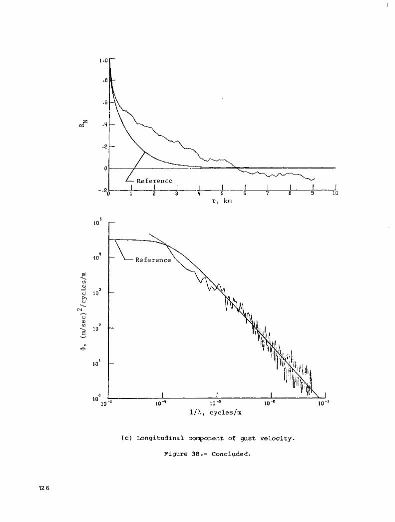
L Reference "

I I I I I I I 1 1 2 3 Y 5 6 7 8 9 10

r, km

1 oo 10

1/X, cyclesfm

(c ) Longitudinal component of gust ve loc i ty .


12 6

L

I I I 1 I 1 2 3 Y 5 6 7 8 9 10

r, km

n Reference


F igure 39.- Power spectra and au tocorre la t ion func t ions €or f l i g h t 32, run 4 .

12 7

L Reference - .20 I I I I I I I 1 2 3 5 6 ' 7 8 3 10

r Y km

r

l/Ay cycleslrn



12 8

I

0

R e f e rence - .20 I I I I I I 1 I I I

1 2 3 5 6 7 8 3 10

I:, km

IOC

10'

loy

10'

102

10' 1(

I/?, , cycles/m



12 9

r, km

1 / A , cycles/m



13 0

r, km

r -

-

-

lop . I I

10 -6 10 -y 10 -’ 10 -2 10 -‘ l/X, cycleslm



131

. ..... ,

L Reference I I I I I I I I I I 1 2 3 9 5 6 7 8 3 10

r, km

I I I 10 -q 10 10 - p

1 / A , cycleslm 10 -1



132

Reference I I I I I I I I 1 I 1 2 3 4 5 6 7 . 8 9 10

r , km

10' I" "I)

I/ X , cycles/m

(a) Vert ical component of gust velocity.

Figure 41.- Power spectra and autocorrelation functions for flight 42, run 2 .

133

L

10'

10

1 o3

lo2

10'

loo 10

r, km

-

10 -q 10 -s 10 -e 10 -' 1/X, cycleslm



134

L' Reference - .20 L"L-"-l-l 1 2 3 Lt 5 I 6 7 I 8 I -U 9 10

r, km

l o r 5

1 / X , cycleslm



135

L Reference I I I 1 I I 1 I I 1 1 2 3 9 5 6 7 8 9 10

* 10

:G 3

1 o2

1 a'

1 oo

10-1 1c

r y km



136

Reference - .20 I 1 I I I 1 1 1 I J 1 2 3 Y 5 6 7 8 9 10

r, km

lo’ r 10’

10

1 o2

lo1

l co 10 -b 10 -y 10” 10 -2 10 -1

1/X, cycles/m



137

0 /

Reference - .20 1 I I I I I I I ! I

1 2 3 Lt 5 6 7 8 9 10

10'

aJ rn ' lo2 e v

h

e

10'

r, km

-

loo 10 -6

loo I 10 -6 10 -' 10 10"

l/X, cycleslm



138

1 OY

3 10

loz

l G 1

loo

10-1 10

- Reference \\


139

-

- .20 I I I I I I. I I 1 1 2 3 't 6 6 7 8 3 10

r, km

-

10 -y 10 -' IO" 10 -' l / h , cycleslm

(b) Lateral component of gust veloc i ty .


140

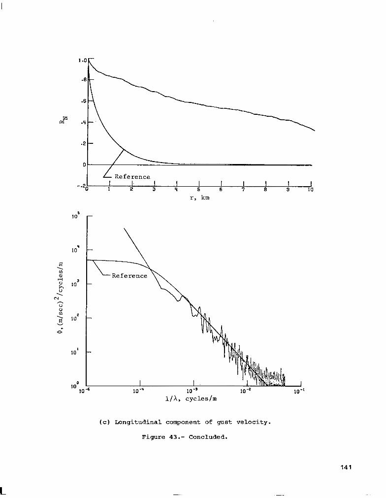
I .OF;-

L Reference I 1 . I I I 1 I I I 1 2 3 9 5 6 7 8 3 10

I

r, km

-6

1 / X , cycles/m



L

141

I 1 I I I I I I J 1. 2 3 Li 5 6 7 8 3 10

r, km

3 io

lo2

10'

1 OC

10" I I I I 10 -5 10 -q 10" 10 4 10"

1/A, cycles/m


F igure 44.- Power spectra and au tocorre la t ion func t ions for f l i g h t 4 2 , run 6.

1 42

I

- .?i I I I I I I I I I I 1 2 3 Lt 5 6 7 8 9 10 - .?i I I I I I I I I I I 1 2 3 Lt 5 6 7 8 9 10

5 10

loy

\ ffl a,

B

2 lo3 u 1

n U a, a 2

N

2 10 W

n

e

10'

11X , cycleslm



143

1 .E

.a

-6

.Y

.2

0

- .2,

1 O6

10'

10%

lo3

1 c2

10' 10

I I I I I I I I I I 1 2 3 Lf 5 6 7 8 9 10

r, km

1 10 -'1 10 -s 10 -* 10 -1

11 X, cycles /m


Figure 44. - Concluded.

144

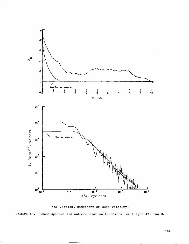
I

2

- .20 I I I I I I 1 I I 1 2 3 Li 5 6 7 8 9 10

7 Reference

10 -* 10 -' 10 -r 10 -1 10 -* 10 -J 10 -=

1/X, cycIes/m

( a ) V e r t i c a l component of gust ve loc i ty .

"I

10 -1

Figure 45.- Power s p e c t r a and au tocor re l a t ion func t ions fo r flight 42, run 8.

145

1 . c

.E

-6

.2

0

- .2,

1 o6

los

n U a, < lo3 v E

lo2

10 -q 10 4 10

l/X, cycleslm 10 -1

(b) L a t e r a l c o m p o n e n t of gust v e l o c i t y .

Figure 45. - C o n t i n u e d .

146

I

I I I I I I I I I J 1 2 3 5 6 7 8 9 10

r, km

11 X, cycleslm



147

.E

.E

&Z .Y

.2

0

- .2

I OS

10 Y

IO'

1 oo 10

- L Reference I I I I

1 2 3 '1 5 6 7 8 3 10 r, km

10 -I 10 -' 10 10 -' I f A , cycles/m

(a) V e r t i c a l component of gus t ve loc i ty .

Figure 46.- Power spec t ra and au tocorre la t ion func t ions €or f l i g h t 42, run 9.

1 .o

-6

.2

0

- .2,

5 10

’1 10

10’

lo2

10’

0 10

r, km

10 -‘1 10 - 3

11 X, cycleslm 10 -1



149

I I

I . o r

- .20[ 1 I 2 3 I I I I I I I I 5 6 7 8 3 10

r, km

1/A, cycles/rn

(c ) Longitudinal component of gus t ve loc i ty .


150

-15 t

-1s L I I I I I

0 1 2 3 tl 5 6 7 8 9 10 11 12 13 ilf 15 I I I I I I I I I I I I I I I I I I I I I I I I I I I I I I I I I I I I I I I I I I I I I I I I I I I I I I I I I I I I I I I I I I I I I I

Time, m i n

( a ) F l igh t 2 0 , run 1.

Figure 47.- Time h i s t o r i e s of mountain waves a t an a l t i t u d e of 1924 m (6311 f t ) .

15

0

-15 t

0

-15 E

-15 L I I I I I

0 1 2 3 Lf 5 6 7 8 9 10 I I I I I I I I I I 1 I I I I I I I I I I I I I I I I I I I I I I I I I I I I I I I I I I

Time, min

(bl F l i g h t 20, run 2.


1 52

-15 i

-15 t

-15 t Time, min

( c ) F l i g h t 20, run 3 .


1 53

I1 "" . __. _ _ _ _ . . . .-

I s F

"5 L

I 1 l l l l l 1 l H l l I I I I I I I I I I I I I I I I I I I I I I I I I I I I I I 0 1 2 3 Lf 5 6 7 .s 9 10

Time, min

(d) F l i g h t 20, run 4.


L-

-15 L

15

-15 L

Time, min (e) Flight 20, run 5.


155

15

0

-15

L A

-15 t 15 r

-15 t I I I I I

Time, min 0 1 2 3 L i 5

I I I I I I I I I I I I I I I I I I I I

Figure 48.- Time histories of mountain waves at an altitude of about 14 000 m (x46 000 ft). Flight 30, run 3.

156

I-

-15 L

-15 i

-1s i

Time, min

( a ) F l i g h t 38, run 3.

Figure 49.- Time h i s t o r i e s of jet stream with long-wavelength effects a t an a l t i t u d e of about 10 700 m (-35 000 f t ) .

157

I

t

t 0

t

-15 t Time, min

F i g u r e 49. - C o n t i n u e d .

158

I

F

-15 L

F

Time, min

( c ) F l i g h t 38, run 6.


159

L

F

-15 i Ti me, min

( d ) F l i g h t 35, run 7 .


160

IIIII I I 1 Ill1 P i .F

I I I I I I llIIlIllllIIll1l111llIII~.1 1l1l1l11ll1l1l11lIIllI

I

1. Report No. 2. Government Accession No.

NASA TP-1979 ~ .

4. Title and Subtitle POWER SPECTRAL MEASUREMENTS OF CLEAR-AIR TURBULENCE TO LONG WAVELENGTHS FOR ALTITUDES UP TO 14 000 METERS

7. Author(s1

Harold N. Murrow, William E. McCain, and Richard H. Rhyne

9. Performing Organization Name and Address

NASA Langley Research Center Hampton, VA 23665

12. Sponsoring Agency Name and Address

National Aeronautics and Space Administration Washington, DC 20546

15. Supplementary Notes

3. Recipient's Catalog No.

5. Report Date ~ "

April 1982 6. Performing Organization Code

505-44-23-06

8. Performing Organization Report No.

L- 14820

10. Work Unit No.

11. Contract or Grant No.

13. Type of Repon and Period Covered

Technical Paper 14. Sponsoring Agency Code

16. Abstract

Measurements of three components of clear-air atmospheric turbulence have been made with an airplane incorporating a special instrumentation system to provide accurate data resolution to wavelengths of approximately 1 2 500 m ( 4 0 000 ft). Flight samplings covered an altitude range from approximately 500 to 14 000 m (1500 to 46 000 ft) in various meteorological conditions. This report presents individual autocorrelation functions and power spectra for the three turbulence components from 43 data runs taken primarily from mountain-wave and jet-stream encounters. The flight location (Eastern or Western United States), date, time, run length, intensit1 level (standard deviation), and values of statistical degrees of freedom for each rur are provided in tabular form. The data presented in this report, along with detailec meteorological descriptions for each sampling flight presented in previously published reports, should provide adequate information for detailed meteorological correlations. Some time histories which contain predominant low-frequency wave motion are also presented.

7. Key Words (Suggested by Author(s1) 18. Distribution Statement

Atmospheric turbulence

Autocorrelation functions Power spectra

Unclassified - Unlimited

Subject Category 47

19. Security Clasif. (of this report) 20. Security Classif. (of this page) 21. No. of Pages 22. Price

Unclassified Unclassified 16 1 A0 8

For Sale by the National Technical Information Service, Sprlnefield. Virginla 22161 NASA-Lanql ey, 1982

Power Spectral Measurements of Clear-Air Turbulence

Documents

Transcript of Power Spectral Measurements of Clear-Air Turbulence