Hypothesis Generation

Hermann Moisl

University of Newcastle

1.0 INTRODUCTION

The aim of science is to understand reality. An academic discipline,

philosophy of science, is devoted to explicating the nature of science and its

relationship to reality, and, perhaps predictably, both are controversial; for an

excellent introduction to the issues see (Chalmers 1999). In practice,

however, most scientists explicitly or implicitly assume a view of scientific

methodology based on the philosophy of Karl Popper (Popper 1959; Popper

1963), in which one or more non-contradictory hypotheses about some

domain of interest are stated, the validity of the hypotheses is tested by

observation of the domain, and the hypotheses are either confirmed (but not

proven) if they are compatible with observation, or rejected if they are not.

Where do such hypotheses come from? In principle it doesn't matter, because

the validity of the claims they make can always be assessed with reference to

the observable state of the world. Any one of us, whatever our background,

could wake up in the middle of the night with an utterly novel and brilliant

hypothesis that, say, unifies quantum mechanics and Einsteinian relativity, but

this kind of inspiration is highly unlikely and must be exceedingly rare. In

practice, scientists develop hypotheses in something like the following

sequence of steps: the researcher (i) selects some aspect of reality that s/he

wants to understand, (ii) becomes familiar with the selected research domain

by observation of it, reads the associated research literature, and formulates a

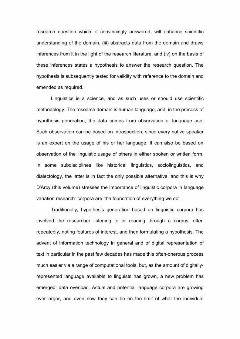
research question which, if convincingly answered, will enhance scientific

understanding of the domain, (iii) abstracts data from the domain and draws

inferences from it in the light of the research literature, and (iv) on the basis of

these inferences states a hypothesis to answer the research question. The

hypothesis is subsequently tested for validity with reference to the domain and

emended as required.

Linguistics is a science, and as such uses or should use scientific

methodology. The research domain is human language, and, in the process of

hypothesis generation, the data comes from observation of language use.

Such observation can be based on introspection, since every native speaker

is an expert on the usage of his or her language. It can also be based on

observation of the linguistic usage of others in either spoken or written form.

In some subdisciplines like historical linguistics, sociolinguistics, and

dialectology, the latter is in fact the only possible alternative, and this is why

D'Arcy (this volume) stresses the importance of linguistic corpora in language

variation research: corpora are 'the foundation of everything we do'.

Traditionally, hypothesis generation based on linguistic corpora has

involved the researcher listening to or reading through a corpus, often

repeatedly, noting features of interest, and then formulating a hypothesis. The

advent of information technology in general and of digital representation of

text in particular in the past few decades has made this often-onerous process

much easier via a range of computational tools, but, as the amount of digitally-

represented language available to linguists has grown, a new problem has

emerged: data overload. Actual and potential language corpora are growing

ever-larger, and even now they can be on the limit of what the individual

researcher can work through efficiently in the traditional way. Moreover, as we

shall see, data abstracted from such large corpora can be impenetrable to

understanding. One approach to the problem is to deal only with corpora of

tractable size, or, equivalently, with tractable subsets of large corpora, but

ignoring potential data in so unprincipled a way is not scientifically

respectable. The alternative is to use mathematically-based computational

tools for data exploration developed in the physical and social sciences,

where data overload has long been a problem. This latter alternative is the

one explored here. Specifically, the discussion shows how a particular type of

computational tool, cluster analysis, can be used in the formulation of

hypotheses in corpus-based linguistic research.

The discussion is in three main parts. The first describes data

abstraction from corpora, the second outlines the principles of cluster

analysis, and the third shows how the results of cluster analysis can be used

in the formulation of hypotheses. Examples are based on the Newcastle

Electronic Corpus of Tyneside English (NECTE), a corpus of dialect speech

(Allen et al. 2007). The overall approach is introductory, and as such the aim

has been to make the material accessible to as broad a readership as

possible.

2. DATA CREATION

'Data' comes from the Latin verb 'to give' and means 'things that are

given'. Data are therefore things to be accepted at face value, true statements

about the world. What is a true statement about the world? That question has

been debated in philosophical metaphysics since Antiquity and probably

before (Bunnin and Yu 2009; Flew and Priest 2002; Zalta 2009), and, in our

own time, has been intensively studied by the disciplines that comprise

cognitive science (for example Thagard 2005). The issues are complex,

controversy abounds, and the associated academic literatures are vast --

saying what a true statement about the world might be is anything but

straightforward. We can't go into all this, and so will adopt the attitude

prevalent in most areas of science: data are abstractions of what we observe

using our senses, often with the aid of instruments (Chalmers 1999).

Data are ontologically different from the world. The world is as it is;

data are an interpretation of it for the purpose of scientific study. The weather

is not the meteorologist’s data –measurements of such things as air

temperature are. A text corpus is not the linguist’s data –measurements of

such things as average sentence length are. Data are constructed from

observation of things in the world, and the process of construction raises a

range of issues that determine the amenability of the data to analysis and the

interpretability of the analytical results. The importance of understanding such

data issues in cluster analysis can hardly be overstated. On the one hand,

nothing can be discovered that is beyond the limits of the data itself. On the

other, failure to understand relevant characteristics of data can lead to results

and interpretations that are distorted or even worthless. For these reasons, a

detailed account of data issues is given before moving on to discussion of

analytical methods.

2.1 Formulation of a research question

In general, any aspect of the world can be described in an arbitrary

number of ways and to arbitrary degrees of precision. The implications of this

go straight to the heart of the debate on the nature of science and scientific

theories, but to avoid being drawn into that debate, this discussion adopts the

position that is pretty much standard in scientific practice: the view, based on

Karl Popper's philosophy of science (Popper 1959; Popper 1963; Chalmers

1999), that there is no theory-free observation of the world. In essence, this

means that there is no such thing as objective observation in science. Entities

in a domain of inquiry only become relevant to observation in terms of a

hypothesis framed using the ontology and axioms of a theory about the

domain. For example, in linguistic analysis, variables are selected in terms of

the discipline of linguistics broadly defined, which includes the division into

subdisciplines such as sociolinguistics and dialectology, the subcategorization

within subdisciplines such as phonetics through syntax to semantics and

pragmatics in formal grammar, and theoretical entities within each

subcategory such as phonemes in phonology and constituency structures in

syntax. Claims, occasionally seen, that the variables used to describe a

corpus are 'theoretically neutral' are naive: even word categories like 'noun'

and 'verb' are interpretative constructs that imply a certain view of how

language works, and they only appear to be theory-neutral because of

familiarity with long-established tradition.

Data can, therefore, only be created in relation to a research question

that is defined on the domain of interest, and that thereby provides an

interpretative orientation. Without such an orientation, how does one know

what to observe, what is important, and what is not?

The domain of interest in the present case is the Newcastle Electronic

Corpus of Tyneside English (NECTE), a corpus of dialect speech interviews

from Tyneside in North-East England1 (Allen et al. 2007).

Figure 1

Moisl et al. (2006) and Moisl and Maguire (2008) have begun the study of the

NECTE corpus with the aim of generating hypotheses about phonetic

variation among speakers in the Tyneside dialect area using cluster analysis.

The research question asked in that work, and which serves as the basis for

what follows here, is:

Is there systematic phonetic variation in the Tyneside speech

community, and , if so, what are the main phonetic determinants of

that variation?

These studies went on to correlate the findings with social data about the

speakers, but the present discussion does not engage with that.

2.2 Variable selection

Given that data are an interpretation of some domain of interest, what

does such an interpretation look like? It is a description of entities in the

domain in terms of variables. A variable is a symbol, and as such is a physical

entity with a conventional semantics, where a conventional semantics is

understood as one in which the designation of a physical thing as a symbol

together with the connection between the symbol and what it represents are

1 http://www.ncl.ac.uk/necte/

determined by agreement within a community. The symbol ‘A’, for example,

represents the phoneme /a/ by common assent, not because there is any

necessary connection between it and what it represents. Since each variable

has a conventional semantics, the set of variables chosen to describe entities

constitutes the template in terms of which the domain is interpreted. Selection

of appropriate variables is, therefore, crucial to the success of any data

analysis.

Which variables are appropriate in any given case? That depends on

the nature of the research question. The fundamental principle in variable

selection is that the variables must describe all and only those aspects of the

domain that are relevant to the research question. In general, this is an

unattainable ideal. Any domain can be described by an essentially arbitrary

number of finite sets of variables; selection of one particular set can only be

done on the basis of personal knowledge of the domain and of the body of

scientific theory associated with it, tempered by personal discretion. In other

words, there is no algorithm for choosing an optimally relevant set of variables

for a research question.

Which variables are suitable to describe the NECTE speakers? In

principle, when setting out to perform a classification of a speech corpus, the

first step is to partition each speaker's analog speech signal into a sequence

of discrete phonetic segments and to represent those segments symbolically,

or, in other words, to transcribe the audio interviews. To do this, one has to

decide which features of the audio signal are of interest, and then to define a

set of variables to represent those features. These decisions were made long

ago with respect to the NECTE interviews.

NECTE is based on two pre-existing corpora, one of them collected in

the late 1960s by the Tyneside Linguistic Survey (TLS) project (Strang 1968;

Pellowe et al. 1972), and the other in 1994 by the Phonological Variation and

Change in Contemporary Spoken English (PVC) project (Milroy et al. 1997).

For present purposes we are interested in the 63 interviews that comprise the

TLS component of NECTE, and it happens that the TLS researchers had

already created phonetic transcriptions of at least part of each interview. This

saved the NECTE project the arduous labour of transcription, but at the same

time bound us to their decisions about which phonetic features are of interest,

and how they should be symbolically represented as variables. Details of the

TLS transcription scheme are available in (Allen et al. 2007) as well as at the

NECTE website2; a short excerpt from the TLS transcription scheme is given

in figure 2 below:

Figure 2

Two levels of transcription were produced, a highly detailed narrow one

designated 'States' in figure 2, and a superordinate ‘Putative Diasystemic

Variables’ (PDV) level which collapsed some of the finer distinctions

transcribed at the ‘States’ level. We shall be dealing with the less detailed

PDV level.

2.3 Variable value assignment

The semantics of each variable determines a particular interpretation of

the domain of interest, and the domain is 'measured' in terms of the

2 http://www.ncl.ac.uk/necte/appendix1.htm

semantics. That measurement constitutes the values of the variables: height

in metres = 1.71, weight in kilograms = 70, and so on. Measurement is

fundamental in the creation of data because it makes the link between data

and the world, and thus allows the results of data analysis to be applied to the

understanding of the world.

Measurement is only possible in terms of some scale. There are

various types of measurement scale, and these are discussed at length in, for

example, any statistics textbook, but for present purposes the main dichotomy

is between numeric and non-numeric. Cluster analysis methods assume

numeric measurement as the default case, and for that reason the same is

assumed in what follows. Specifically, we shall be interested in the number of

times each speaker uses each of the NECTE phonetic variables. The

speakers are therefore 'measured' in terms of the frequency with which they

use these segments

2.4 Data representation

If they are to be analyzed using mathematically-based computational

methods, the descriptions of the entities in the domain of interest in terms of

the selected variables must be mathematically represented. A widely used

way of doing this, and the one adopted here, is to use structures from a

branch of mathematics known as linear algebra. There are numerous

textbooks and websites devoted to linear algebra; a small selection of

introductory textbooks is (Anton 2005; Poole 2005; Blyth and Robertson

2002).

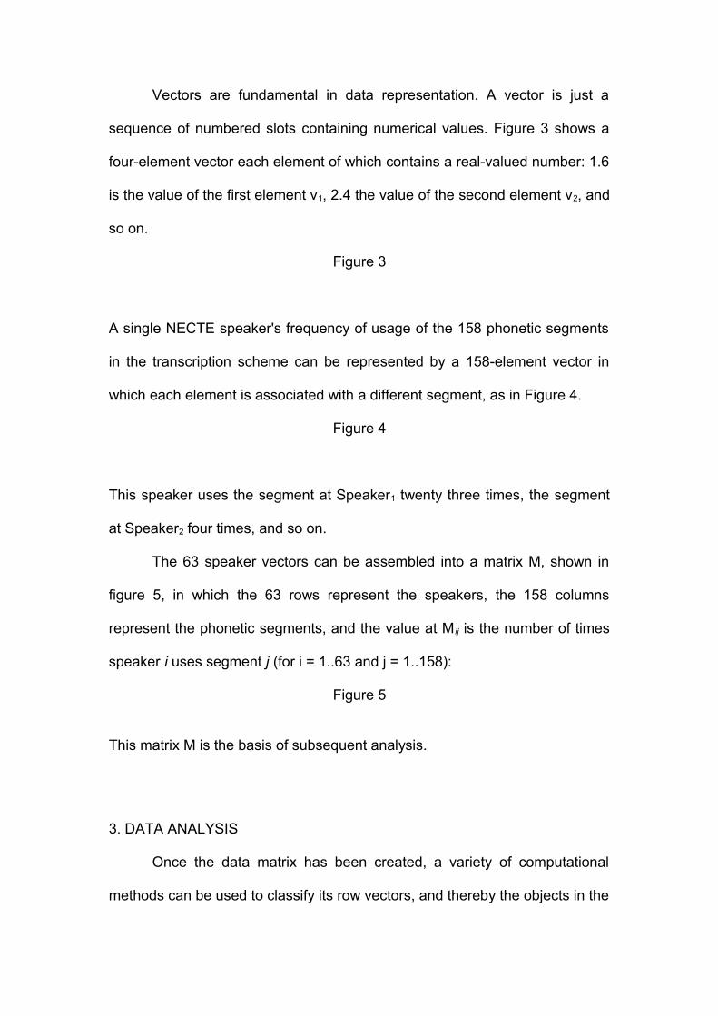
Vectors are fundamental in data representation. A vector is just a

sequence of numbered slots containing numerical values. Figure 3 shows a

four-element vector each element of which contains a real-valued number: 1.6

is the value of the first element v1, 2.4 the value of the second element v2, and

so on.

Figure 3

A single NECTE speaker's frequency of usage of the 158 phonetic segments

in the transcription scheme can be represented by a 158-element vector in

which each element is associated with a different segment, as in Figure 4.

Figure 4

This speaker uses the segment at Speaker1 twenty three times, the segment

at Speaker2 four times, and so on.

The 63 speaker vectors can be assembled into a matrix M, shown in

figure 5, in which the 63 rows represent the speakers, the 158 columns

represent the phonetic segments, and the value at M ij is the number of times

speaker i uses segment j (for i = 1..63 and j = 1..158):

Figure 5

This matrix M is the basis of subsequent analysis.

3. DATA ANALYSIS

Once the data matrix has been created, a variety of computational

methods can be used to classify its row vectors, and thereby the objects in the

domain that the row vectors represent. In the present case, those objects are

the NECTE speakers. The discussion is in 4 main parts:

Part 1 motivates the use of computational methods for clustering.

Part 2 introduces a fundamental concept: vector space.

Part 3 describes how clusters can be found in vector space.

Part 4 deals with some issues that arise in clustering.

All four parts of the discussion are based on the NECTE data matrix M

developed in the preceding section.

3.1 Motivation

We have seen that creation of data for study of a domain requires

description of the objects in the domain in terms of variables. One might

choose to observe only one aspect -the height of individuals in a population,

say- in which case the data consists of more or less numerous values

assigned to one variable; such data is univariate. If two values are observed

-say height and weight- then the data is bivariate, if three trivariate, and so on

up to some arbitrary number n; any data where n is greater than 1 is

multivariate.

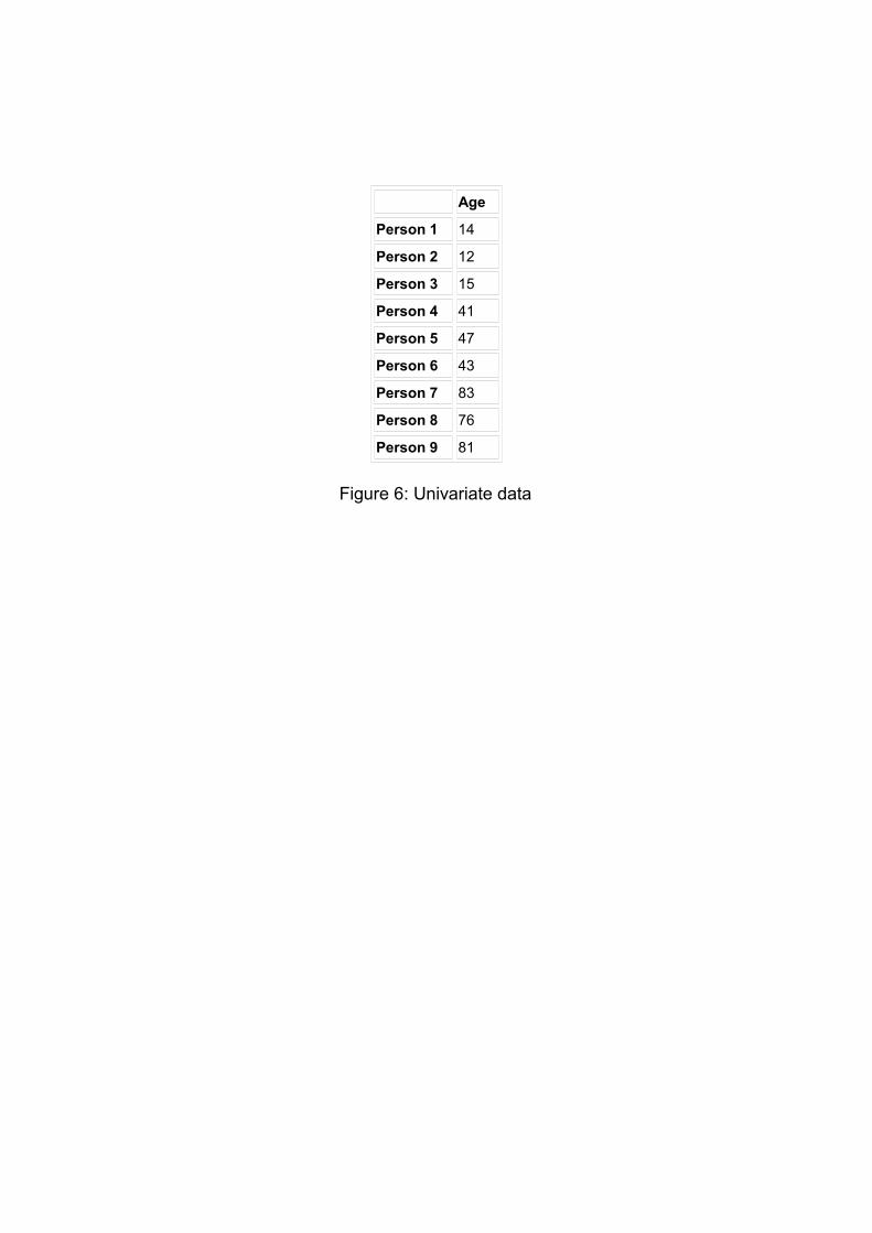
As the number of variables grows, so does the difficulty of classifying

the objects that the data matrix rows represent by direct inspection. Consider,

for example, figure 6, which shows a matrix describing nine people in terms of

a single variable Age.

Figure 6

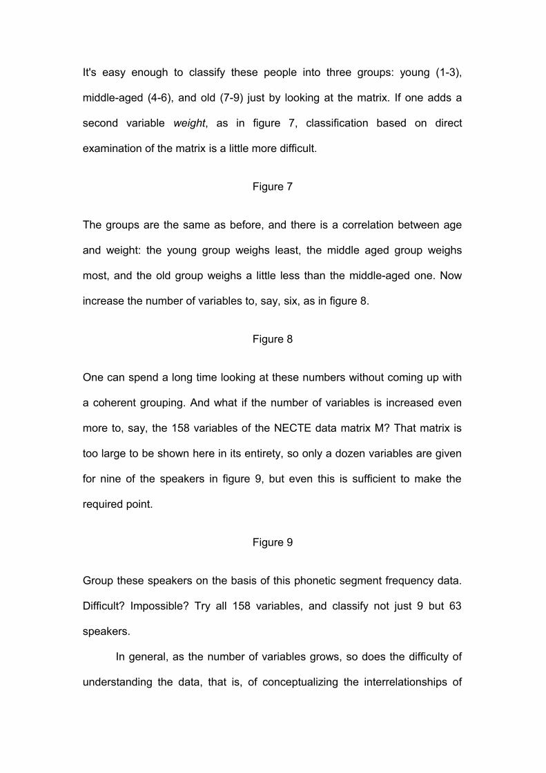
It's easy enough to classify these people into three groups: young (1-3),

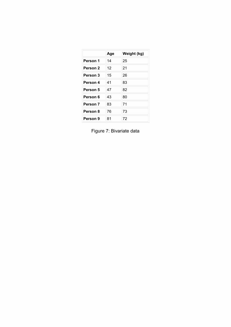
middle-aged (4-6), and old (7-9) just by looking at the matrix. If one adds a

second variable weight, as in figure 7, classification based on direct

examination of the matrix is a little more difficult.

Figure 7

The groups are the same as before, and there is a correlation between age

and weight: the young group weighs least, the middle aged group weighs

most, and the old group weighs a little less than the middle-aged one. Now

increase the number of variables to, say, six, as in figure 8.

Figure 8

One can spend a long time looking at these numbers without coming up with

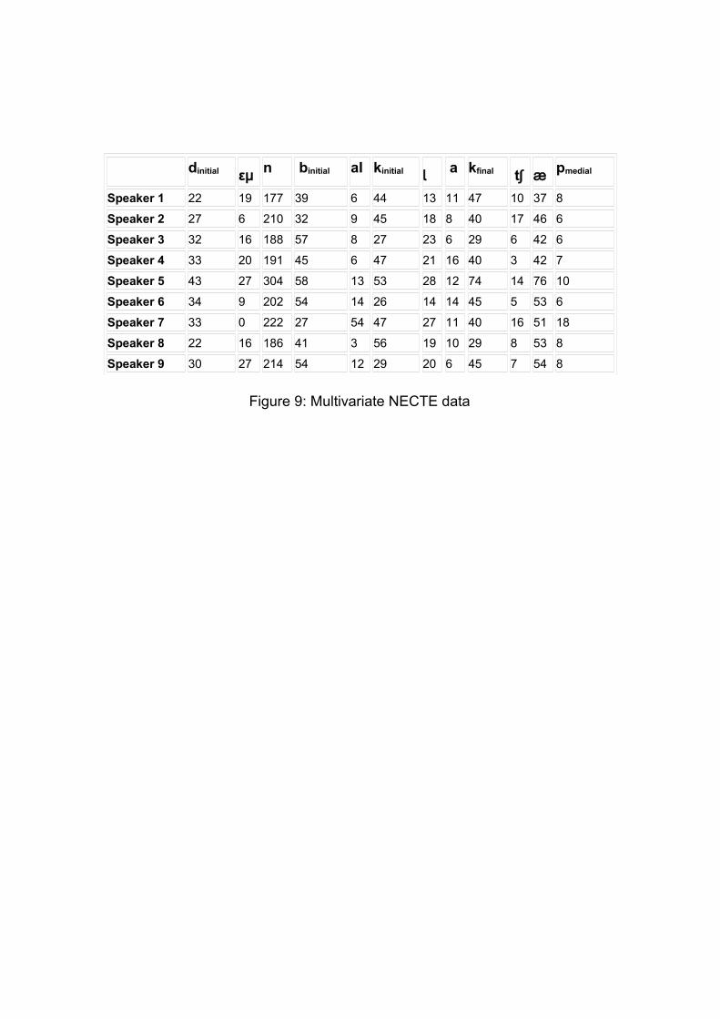
a coherent grouping. And what if the number of variables is increased even

more to, say, the 158 variables of the NECTE data matrix M? That matrix is

too large to be shown here in its entirety, so only a dozen variables are given

for nine of the speakers in figure 9, but even this is sufficient to make the

required point.

Figure 9

Group these speakers on the basis of this phonetic segment frequency data.

Difficult? Impossible? Try all 158 variables, and classify not just 9 but 63

speakers.

In general, as the number of variables grows, so does the difficulty of

understanding the data, that is, of conceptualizing the interrelationships of

variables within a single data item on the one hand, and the interrelationships

of complete data items on the other. The moral is straightforward: human

cognitive makeup is unsuited to seeing regularities in anything but the

smallest collections of numerical data. To see the regularities we need

graphical aids, and that is what clustering methods provide.

3.2 Vector space

Though it is just a sequence of numbers, a vector can be geometrically

interpreted (Anton 2005; Poole 2005; Blyth and Robertson 2002). To see how,

take a vector consisting of two elements, say v = (30,70). Under a geometrical

interpretation, the two elements of v define a two-dimensional space, the

numbers at v1 = 30 and v2 = 70 are coordinates in that space, and the vector v

itself is a point at the coordinates (30,70), as shown in figure 10.

Figure 10

A vector consisting of three elements, say v = (40, 20, 60) defines a three-

dimensional space in which the coordinates of the point v are 40 along the

horizontal axis, 20 along the vertical axis, and 60 along the third axis shown in

perspective, as in figure 11.

Figure 11

A vector v = (22, 38, 52, 12) defines a four-dimensional space with a point at

the stated coordinates, and so on to any dimensionality n. Vector spaces of

dimensionality greater than 3 are impossible to visualize directly and are

therefore counterintuitive, but mathematically there is no problem with them;

two and three dimensional spaces are useful as a metaphor for

conceptualizing higher-dimensional ones.

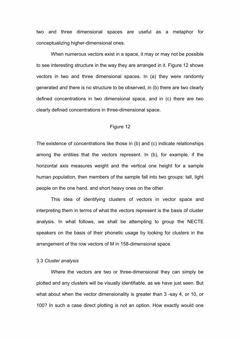
When numerous vectors exist in a space, it may or may not be possible

to see interesting structure in the way they are arranged in it. Figure 12 shows

vectors in two and three dimensional spaces. In (a) they were randomly

generated and there is no structure to be observed, in (b) there are two clearly

defined concentrations in two dimensional space, and in (c) there are two

clearly defined concentrations in three-dimensional space.

Figure 12

The existence of concentrations like those in (b) and (c) indicate relationships

among the entities that the vectors represent. In (b), for example, if the

horizontal axis measures weight and the vertical one height for a sample

human population, then members of the sample fall into two groups: tall, light

people on the one hand, and short heavy ones on the other.

This idea of identifying clusters of vectors in vector space and

interpreting them in terms of what the vectors represent is the basis of cluster

analysis. In what follows, we shall be attempting to group the NECTE

speakers on the basis of their phonetic usage by looking for clusters in the

arrangement of the row vectors of M in 158-dimensional space.

3.3 Cluster analysis

Where the vectors are two or three-dimensional they can simply be

plotted and any clusters will be visually identifiable, as we have just seen. But

what about when the vector dimensionality is greater than 3 -say 4, or 10, or

100? In such a case direct plotting is not an option. How exactly would one

draw a 6-dimensional space, for example? Many data matrix row vectors have

dimensionalities greater than 3 -the NECTE matrix M has dimensionality 158-

and, to identify clusters in such high-dimensional spaces some procedure

more general than direct plotting is required. A variety of such procedures is

available, and they are generically known as cluster analysis methods. This

section looks at these methods.

The literature on cluster analysis is extensive. A few recent books are

(Everitt 2001; Kaufman and Rousseeuw 2005), but many textbooks in fields like

multivariate statistical analysis, information retrieval, and data mining also

contain useful and accessible discussions, and there are numerous relevant

and often excellent websites.

The discussion of cluster analysis is in four parts. The first introduces

distance in vector space, the second describes one particular class of

clustering methods, the third applies that type of method to the NECTE data

matrix M, and the fourth interprets the result of the NECTE analysis.

3.3.1 Distance in vector space

Where there are two or more vectors in a space, it is possible to

measure the distance between any two of them and to rank them in terms of

their proximity to one another. Figure 13 shows a simple case of a 2-

dimensional space in which the distance from vector A to vector B is greater

than the distance from A to C.

Figure 13

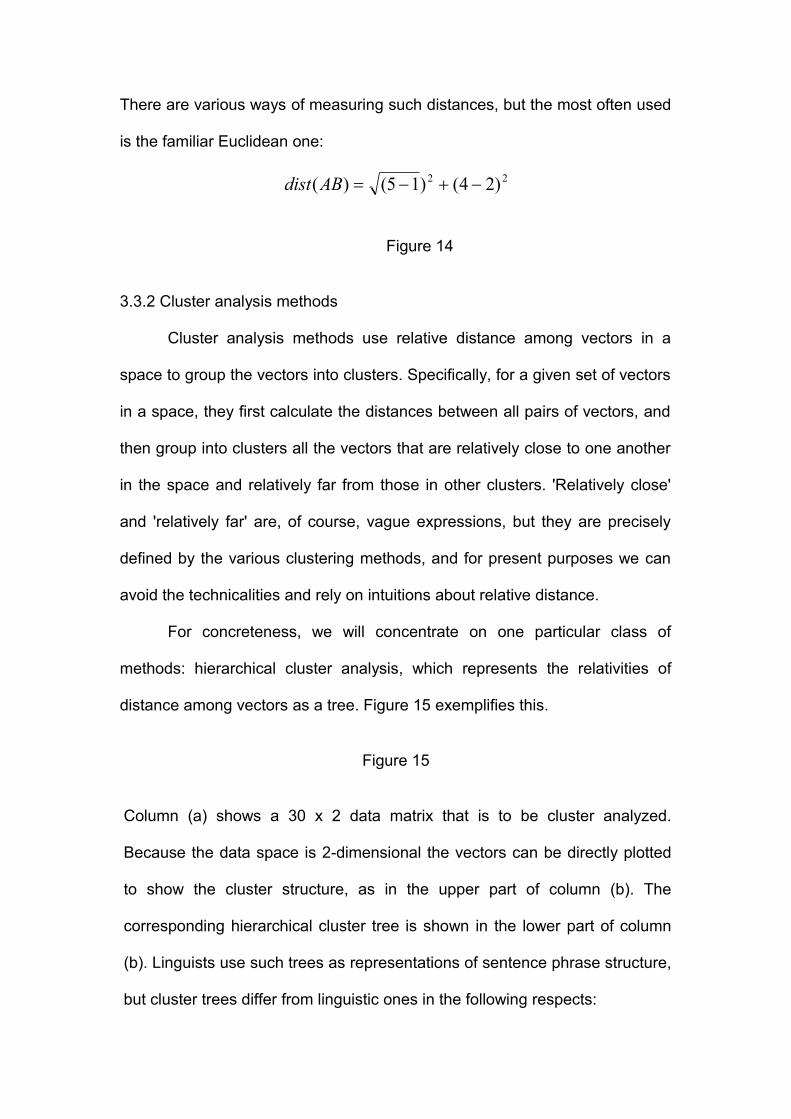
There are various ways of measuring such distances, but the most often used

is the familiar Euclidean one:

22 )24()15()( ABdist

Figure 14

3.3.2 Cluster analysis methods

Cluster analysis methods use relative distance among vectors in a

space to group the vectors into clusters. Specifically, for a given set of vectors

in a space, they first calculate the distances between all pairs of vectors, and

then group into clusters all the vectors that are relatively close to one another

in the space and relatively far from those in other clusters. 'Relatively close'

and 'relatively far' are, of course, vague expressions, but they are precisely

defined by the various clustering methods, and for present purposes we can

avoid the technicalities and rely on intuitions about relative distance.

For concreteness, we will concentrate on one particular class of

methods: hierarchical cluster analysis, which represents the relativities of

distance among vectors as a tree. Figure 15 exemplifies this.

Figure 15

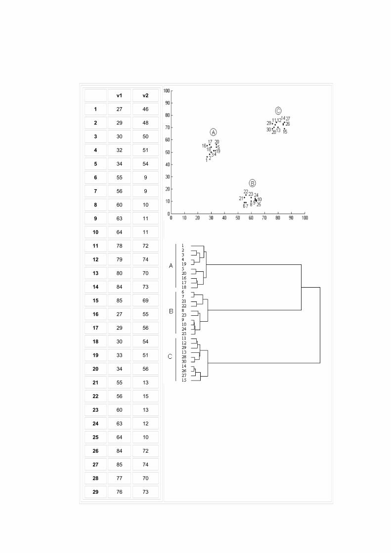
Column (a) shows a 30 x 2 data matrix that is to be cluster analyzed.

Because the data space is 2-dimensional the vectors can be directly plotted

to show the cluster structure, as in the upper part of column (b). The

corresponding hierarchical cluster tree is shown in the lower part of column

(b). Linguists use such trees as representations of sentence phrase structure,

but cluster trees differ from linguistic ones in the following respects:

The leaves are not lexical tokens but labels for the data items -the

numbers at the leaves correspond to the numerical labels of the row

vectors in the data matrix.

They represent not grammatical constituency but relativities of distance

between clusters. The lengths of the branches linking the clusters

represent degrees of closeness: the shorter the branch, the more similar

the clusters. In cluster A vectors 4 and 19 are very close and thus linked

with very short lines; 2 and 3 are almost but not quite as close as 4 and

19, and are therefore linked with slightly longer lines, and so on.

Knowing this, the tree can be interpreted as follows. There are three clusters

labelled A, B, and C in each of which the distances among vectors are quite

small. These three clusters are relatively far from one another, though A and

B are closer to one another than either of them is to C. Comparison with the

vector plot shows that the hierarchical analysis accurately represents the

distance relations among the 30 vectors in 2-dimensional space.

Given that the tree tells us nothing more than what the plot tells us,

what is gained? In the present case, nothing. The real power of hierarchical

analysis lies in its independence of vector space dimensionality. We have

seen that direct plotting is limited to three or fewer dimensions, but there is no

dimensionality limit on hierarchical analysis -it can determine relative

distances in vector spaces of any dimensionality and represent those distance

relativities as a tree like the one above. To exemplify this, the 158-

dimensional NECTE data matrix M was hierarchically cluster analyzed, and

the results of the analysis are shown in the next section.

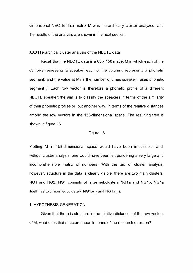
3.3.3 Hierarchical cluster analysis of the NECTE data

Recall that the NECTE data is a 63 x 158 matrix M in which each of the

63 rows represents a speaker, each of the columns represents a phonetic

segment, and the value at Mij is the number of times speaker i uses phonetic

segment j. Each row vector is therefore a phonetic profile of a different

NECTE speaker; the aim is to classify the speakers in terms of the similarity

of their phonetic profiles or, put another way, in terms of the relative distances

among the row vectors in the 158-dimensional space. The resulting tree is

shown in figure 16.

Figure 16

Plotting M in 158-dimensional space would have been impossible, and,

without cluster analysis, one would have been left pondering a very large and

incomprehensible matrix of numbers. With the aid of cluster analysis,

however, structure in the data is clearly visible: there are two main clusters,

NG1 and NG2; NG1 consists of large subclusters NG1a and NG1b; NG1a

itself has two main subclusters NG1a(i) and NG1a(ii).

4. HYPOTHESIS GENERATION

Given that there is structure in the relative distances of the row vectors

of M, what does that structure mean in terms of the research question?

'Is there systematic phonetic variation in the Tyneside speech

community, and, if so, what are the main phonetic determinants of

that variation?'.

Because the row vectors of M are phonetic profiles of the NECTE speakers,

the cluster structure means that the speakers fall into clearly defined groups

with specific interrelationships rather than, say, being randomly distributed

around the phonetic space. A reasonable hypothesis to answer the first part of

the research question, therefore, is that there is systematic variation in the

Tyneside speech community. This hypothesis can be refined by examining

the social data relating to the NECTE speakers, which shows, for example,

that all those in the NG1 cluster come from the Gateshead area on the south

side of the river Tyne and all those in NG2 come from Newcastle on the north

side, and that the subclusters in NG1 group the Gateshead speakers by

gender and occupation.

The cluster tree can also be used to generate a hypothesis in answer

to the second part of the research question. So far we know that the NECTE

speakers fall into clearly-demarcated groups on the basis of variation in their

phonetic usage. We do not, however, know why, that is, which segments out

of the 158 in the TLS transcription scheme are the main determinants of this

regularity. To identify these segments (Moisl & Maguire 2008), we begin by

looking at the two main clusters NG1 and NG2 to see which segments are

most important in distinguishing them.

The first step is to create for the NG1 cluster a vector that captures the

general phonetic characteristics of the speakers it contains, and to do the

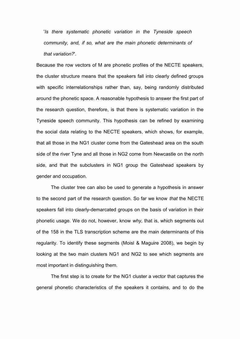
same for the NG2. Such vectors can be created by averaging all the row

vectors in a cluster using the formula

where vj is the jth element of the average or 'centroid' vector v (for j = 1..the

number of columns in M), M is the data matrix, Σ designates summation, and

m is the number of row vectors in the cluster in question (56 for NG1, 7 for

NG2). This yields two centroid vectors.

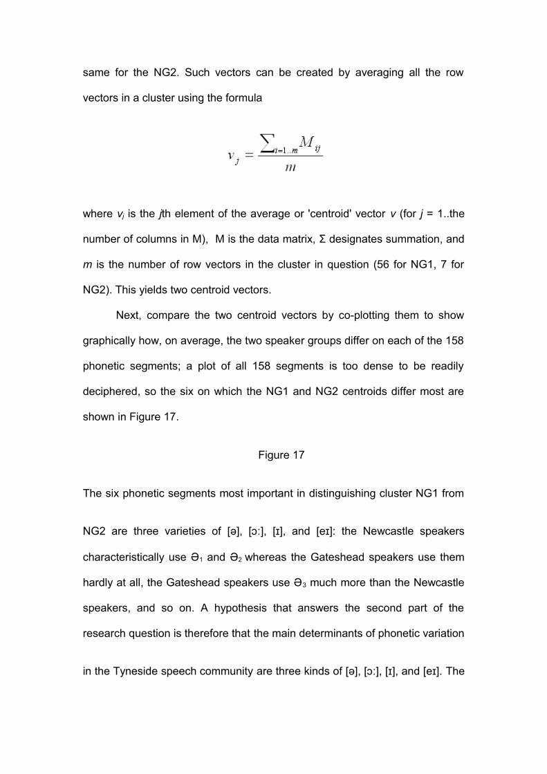
Next, compare the two centroid vectors by co-plotting them to show

graphically how, on average, the two speaker groups differ on each of the 158

phonetic segments; a plot of all 158 segments is too dense to be readily

deciphered, so the six on which the NG1 and NG2 centroids differ most are

shown in Figure 17.

Figure 17

The six phonetic segments most important in distinguishing cluster NG1 from

NG2 are three varieties of [ə], [ɔː], [ɪ], and [eɪ]: the Newcastle speakers

characteristically use Ə1 and Ə2 whereas the Gateshead speakers use them

hardly at all, the Gateshead speakers use Ə3 much more than the Newcastle

speakers, and so on. A hypothesis that answers the second part of the

research question is therefore that the main determinants of phonetic variation

in the Tyneside speech community are three kinds of [ə], [ɔː], [ɪ], and [eɪ]. The

subclusters of NG1 can be examined in the same way and the hypothesis

thereby further refined.

Having formulated two hypotheses about Tyneside speech, they need

to be tested against additional evidence from a source or sources other than

NECTE and emended or even discarded if that is what the evidence requires.

5. SUMMARY

This discussion set out to show how one type of computational

analytical tool, cluster analysis, can be used to generate hypotheses about

large digital linguistic corpora when the data abstracted from them is too

complex to be interpreted by direct inspection. This approach to hypothesis

generation is useful primarily when dealing with corpora in languages that

have been relatively little studied, such as endangered languages, but even

for intensively-studied ones like English, where hypotheses can usually be

generated from the existing research literature, cluster analysis can produce

surprises, as Moisl and Maguire (2008) showed for Tyneside English.

6. WHERE TO GO NEXT

The foregoing discussion was introductory, and anyone wishing to use

cluster analysis in actual research applications has some additional reading to

do. There is no shortage of such reading: the literature on cluster analysis,

both in traditional printed form and on the Web, is extensive. Much of it is,

however, quite technical, and this can be an obstacle to those new to the

subject. It's important to have a secure intuitive grasp of the underlying

concepts before trying to assimilate the technicalities, so a good way into the

literature is to start with the Web, using 'cluster analysis' as the search string.

There are numerous good and even excellent introductory-level cluster

analysis websites, and working through these lays the groundwork for more

advanced reading. Romesburg (1984) is an accessible first textbook, followed

by Everitt et al. (2001); the latter contains an extensive bibliography for further

reading.

Knowing the theory of cluster analysis is a necessary but not sufficient

condition for using it in research. Software is required to do the actual work.

The standard statistics packages available in university and other research

environments include a few types of clustering method, but more specialized

ones provide a greater range of methods and, generally, better output

graphics; a Web search using the string 'cluster analysis software' gives a

good overview of what is available. Also very useful are Web directories of

cluster analysis and related resources such as Fionn Murtagh's Multivariate

Data Analysis Software and Resources Page (http://astro.u-

strasbg.fr/~fmurtagh/mda-sw/).

The data to be cluster analyzed may contain characteristics that can

distort the result or even render it invalid as a basis for hypothesis generation.

These characteristics, which include variation in the lengths of documents in

multi-document corpora, data sparsity, and nonlinearity, must be recognized

and where necessary eliminated or at least mitigated prior to undertaking the

analysis. Given its importance, the research literature contains surprisingly

little on such matters; see Pyle (1999) and Moisl (2007, 2008b, 2010)

Finally, anyone proposing to use cluster analysis has to face the reality

that, to do so respectably, knowledge of the basics of linear algebra and of

statistics is a prerequisite. Some introductory textbooks on linear algebra are

Anton (2005), Blyth (2002), and Poole (2005); introductory statistics textbooks

are too numerous to require individual mention, and are available in any

research library as well as on the Web.

7. THE FUTURE FOR CLUSTER ANALYSIS IN LINGUISTIC VARIATION

STUDIES

Cluster analysis has long been and continues to be a standard data

processing tool across a broad range of physical and social sciences. The

advent of digital electronic text in the second half of the twentieth century has

driven the emergence of research disciplines devoted to search and

interpretation of large digital natural language document collections, among

them Information Retrieval (Manning et al. 2008), Data Mining (Hand et al.

2001), Computational Linguistics (Mitkov 2005), and Natural Language

Processing (Manning and Schütze 1999), and here too cluster analysis is a

standard tool. As increasingly large digital collections become available for

research into linguistic variation, traditional analytical methods will become

intractable, and use of the computational tools developed by these text

processing disciplines, including cluster analysis, will become the only realistic

option.

REFERENCES

Allen, Will, Beal, Joan, Corrigan, Karen, Maguire, Warren, and Moisl,

Hermann 2007. ‘A linguistic time-capsule: The Newcastle Electronic

Corpus of Tyneside English’, in Beal et al. (eds.) 2007, 16-48.

Anton, Howard 2005. Elementary Linear Algebra. 9th ed. Hoboken NJ: Wiley

International.

Beal, Joan, Corrigan, Karen, and Moisl, Hermann 2007 (eds). Creating and

Digitising Language Corpora, Vol. 2: Diachronic Databases. Hampshire

and New York: Palgrave Macmillan.

Blyth, T. and Robertson, Edmund 2002. Basic Linear Algebra. 2nd ed.

Heidelberg and New York: Springer.

Bunnin, Nicholas and Yu, Jiyuan 2009. The Blackwell Dictionary of Western

Philosophy. Hoboken NJ: Wiley Blackwell.

Chalmers, Alan 1999. What is this thing called science? 3rd ed. New York:

McGraw-Hill / Open University Press.

Everitt, Brian, Landau, Sabine and Leese, Morven 2001. Cluster Analysis. 4th

ed. London: Arnold.

Flew, Antony and Priest, Stephen 2002. A Dictionary of Philosophy. 3rd ed.

London: PanMacmillan.

Hand, David, Mannila, Heikki, and Smyth, Padhraic 2001. Principles of Data

Mining. Cambridge MA: MIT Press.

Kaufman, Leonard and Rousseeuw, Peter 2005. Finding Groups in Data. An

Introduction to Cluster Analysis. 2nd ed. Hoboken NJ: Wiley Blackwell.

Manning, Christopher,and Schütze, Hinrich 1999. Foundations of Statistical

Natural Language Processing. Cambridge MA: Cambridge University

Press.

Manning, Christopher, Raghavan, Prabhakar, and Schütze, Hinrich 2008.

Introduction to Information Retrieval. Cambridge: Cambridge University

Press.

Milroy, Lesley, Milroy, Jim and Docherty, Gerry 1997. ‘Phonological variation

and change in contemporary spoken British English’. SRC Unpublished

Final Report, Dept. of Speech, University of Newcastle upon Tyne, UK.

Mitkov, Ruslan 2005. The Oxford Handbook of Computational Linguistics.

Oxford: Oxford University Press.

Moisl, Hermann, Maguire, Warren and Allen Will 2006. 'Phonetic variation in

Tyneside: exploratory multivariate analysis of the Newcastle Electronic

Corpus of Tyneside English', in Hinskens, Frans (ed.) Language Variation.

European Perspectives. Amsterdam: John Benjamins , 127-141.

Moisl, Hermann 2007. 'Data nonlinearity in exploratory multivariate analysis of

language corpora', in Computing and Historical Phonology. Proceedings of

the Ninth Meeting of the ACL Special Interest Group in Computational

Morphology and Phonology, June 28 2007, ed. Nerbonne, John, Ellison,

Mark, and Kondrak, Grzegorz, Association for Computational Linguistics,

93-100. Available online at:

http://www.let.rug.nl/alfa/Prague/proceedings.pdf.

Moisl, Hermann and Maguire, Warren 2008a. 'Identifying the Main

Determinants of Phonetic Variation in the Newcastle Electronic Corpus of

Tyneside English', Journal of Quantitative Linguistics 15: 46-69.

Moisl, Hermann 2008b. 'Exploratory Multivariate Analysis', in Lüdeling, Anke

and Kytö, Merja (eds.) Corpus Linguistics. An International Handbook.

Berlin: Mouton de Gruyter.

Moisl, Hermann 2010. 'Sura length and lexical probability estimation in cluster

analysis of the Qur'an', ACM Transactions on Asian Language Information

Processing (forthcoming).

Pellowe, John, Strang, Barbara, Nixon, Graham and McNeany, Vince 1972. ‘A

dynamic modelling of linguistic variation: the urban (Tyneside) linguistic

survey’, Lingua 30: 1–30.

Poole, David 2005. Linear Algebra: A Modern Introduction. Florence KY:

Brooks Cole.

Popper, Karl 1959. The Logic of Scientific Discovery. New York: Basic Books.

Popper, Karl 1963. Conjectures and Refutations: The Growth of Scientific

Knowledge. Florence KY: Routledge / Taylor & Francis Group.

Pyle, Dorian 1999. Data Preparation for Data Mining. San Francisco: Morgan

Kaufmann.

Romesburg, H. Charles 1984. Cluster Analysis for Researchers. Florence

KY: Wadsworth.

Strang, Barbara 1968. ‘The Tyneside Linguistic Survey’, Zeitschrift für

Mundartforschung, Neue Folge 4: 788–94.

Thagard, Paul 2005. Mind: Introduction to Cognitive Science. 2nd ed.

Cambridge MA: MIT Press.

Zalta, Edward 2009. Stanford Encyclopedia of Philosophy. The Metaphysics

Research Lab, Stanford University, http://plato.stanford.edu/.

WORD COUNT: 6690 (including References)

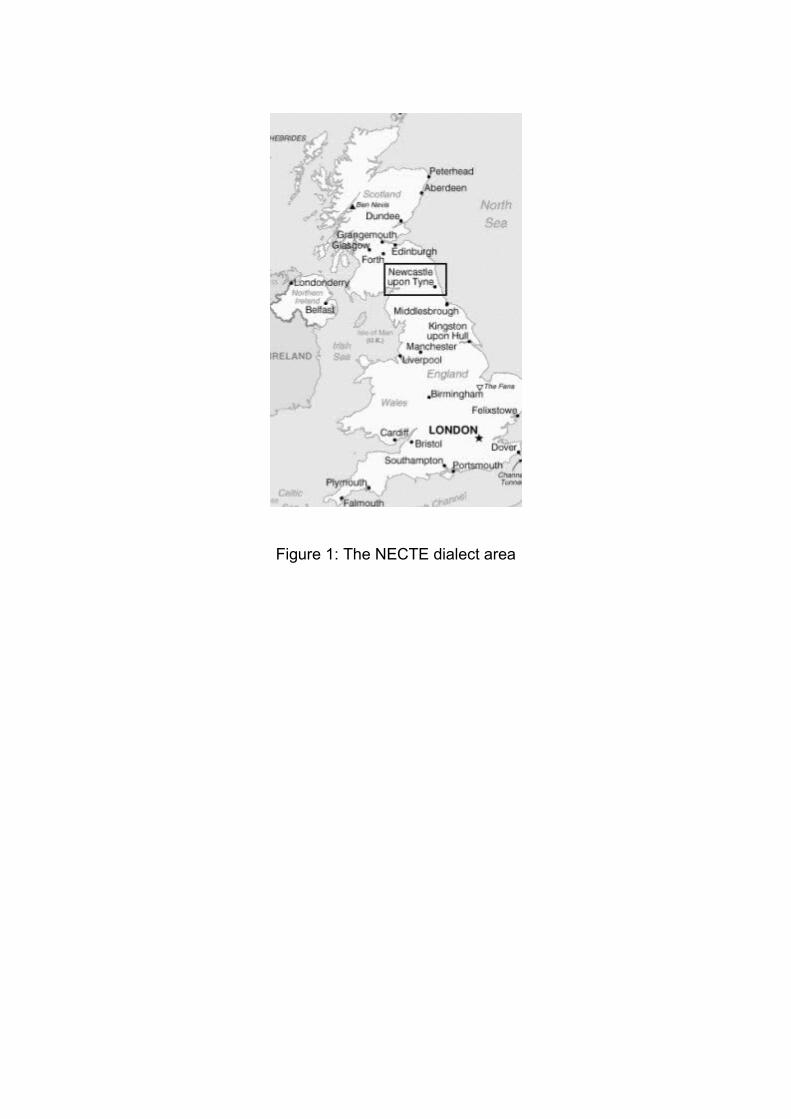
Figure 1: The NECTE dialect area

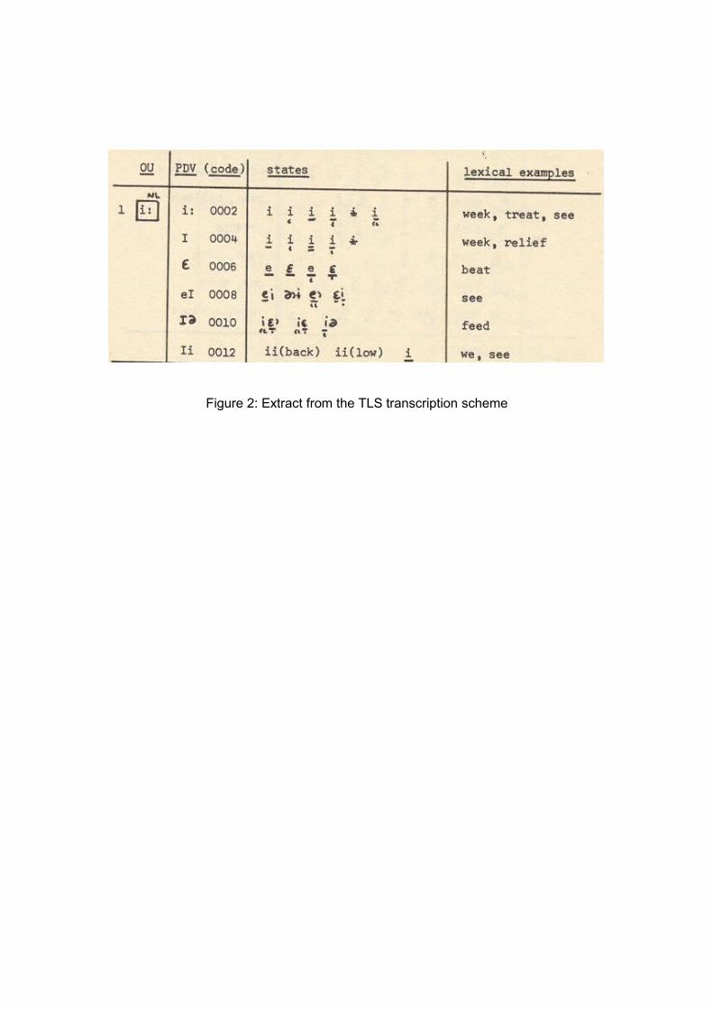
Figure 2: Extract from the TLS transcription scheme

Figure 3: A numerical vector

Figure 4: A NECTE data vector

Figure 5: A fragment of the NECTE data matrix M

Age

Person 1 14

Person 2 12

Person 3 15

Person 4 41

Person 5 47

Person 6 43

Person 7 83

Person 8 76

Person 9 81

Figure 6: Univariate data

Age Weight (kg)

Person 1 14 25

Person 2 12 21

Person 3 15 26

Person 4 41 83

Person 5 47 82

Person 6 43 80

Person 7 83 71

Person 8 76 73

Person 9 81 72

Figure 7: Bivariate data

Age Weight (kg) Height (m) Size of family Years worked Trips abroad

Person 1 14 25 1.4 5 2 2

Person 2 12 21 1.36 5 0 0

Person 3 15 26 1.5 4 1 1

Person 4 41 83 1.74 7 15 46

Person 5 47 82 1.72 3 17 23

Person 6 43 80 1.66 6 21 0

Person 7 83 71 1.65 2 36 12

Person 8 76 73 1.68 5 34 29

Person 9 81 72 1.81 4 42 0

Figure 8: Multivariate data

dinitial εμ n binitial aI kinitial Ɩ a kfinal tʃ æ pmedial

Speaker 1 22 19 177 39 6 44 13 11 47 10 37 8

Speaker 2 27 6 210 32 9 45 18 8 40 17 46 6

Speaker 3 32 16 188 57 8 27 23 6 29 6 42 6

Speaker 4 33 20 191 45 6 47 21 16 40 3 42 7

Speaker 5 43 27 304 58 13 53 28 12 74 14 76 10

Speaker 6 34 9 202 54 14 26 14 14 45 5 53 6

Speaker 7 33 0 222 27 54 47 27 11 40 16 51 18

Speaker 8 22 16 186 41 3 56 19 10 29 8 53 8

Speaker 9 30 27 214 54 12 29 20 6 45 7 54 8

Figure 9: Multivariate NECTE data

Figure 10: A vector in two-dimensional space

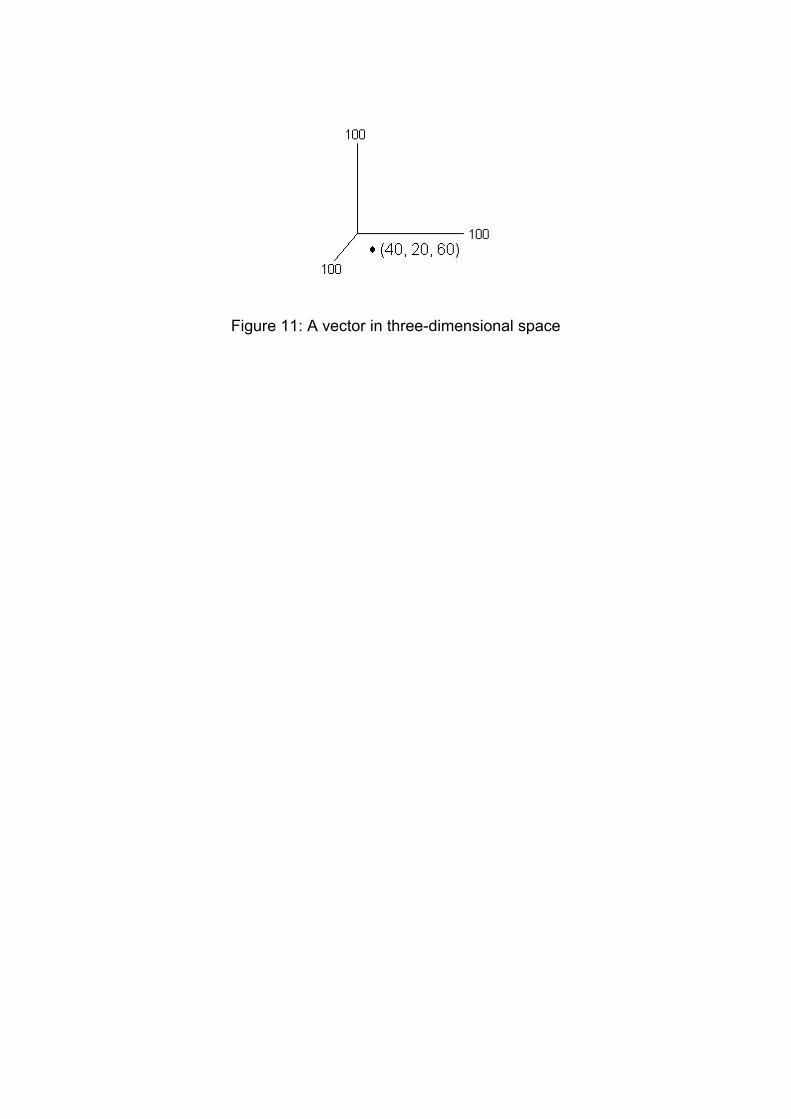
Figure 11: A vector in three-dimensional space

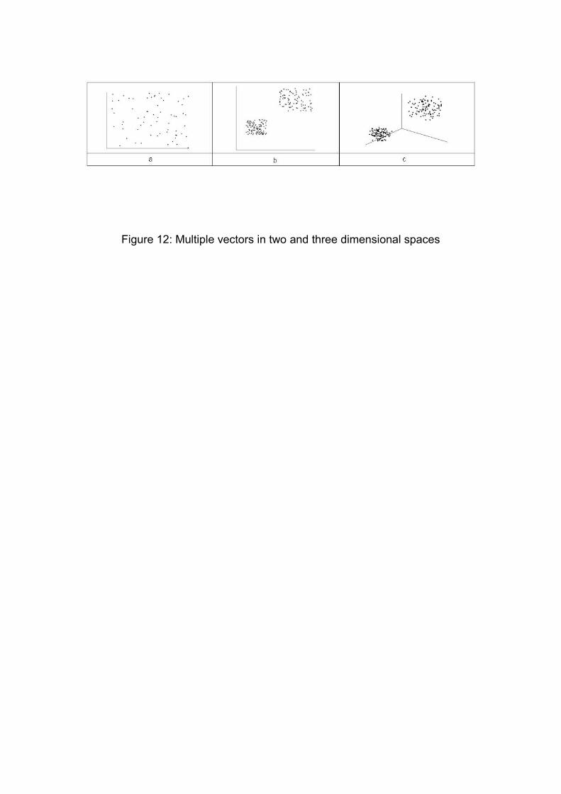
Figure 12: Multiple vectors in two and three dimensional spaces

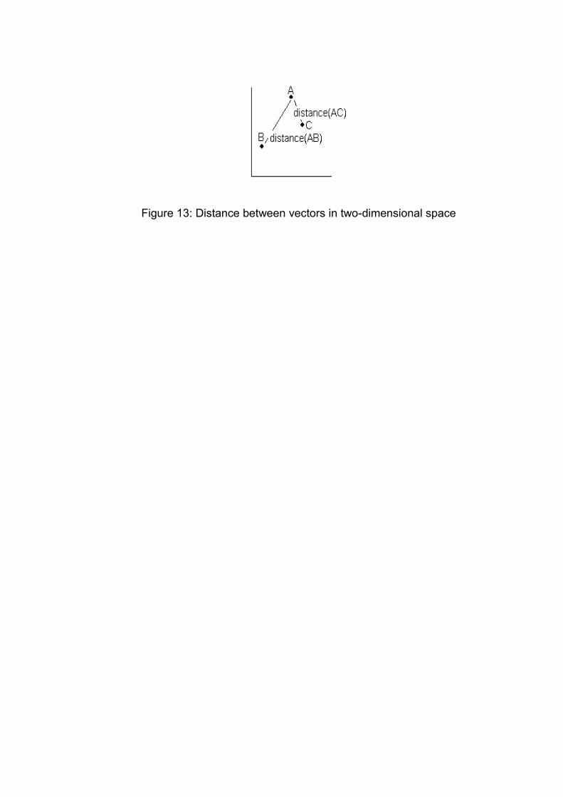
Figure 13: Distance between vectors in two-dimensional space

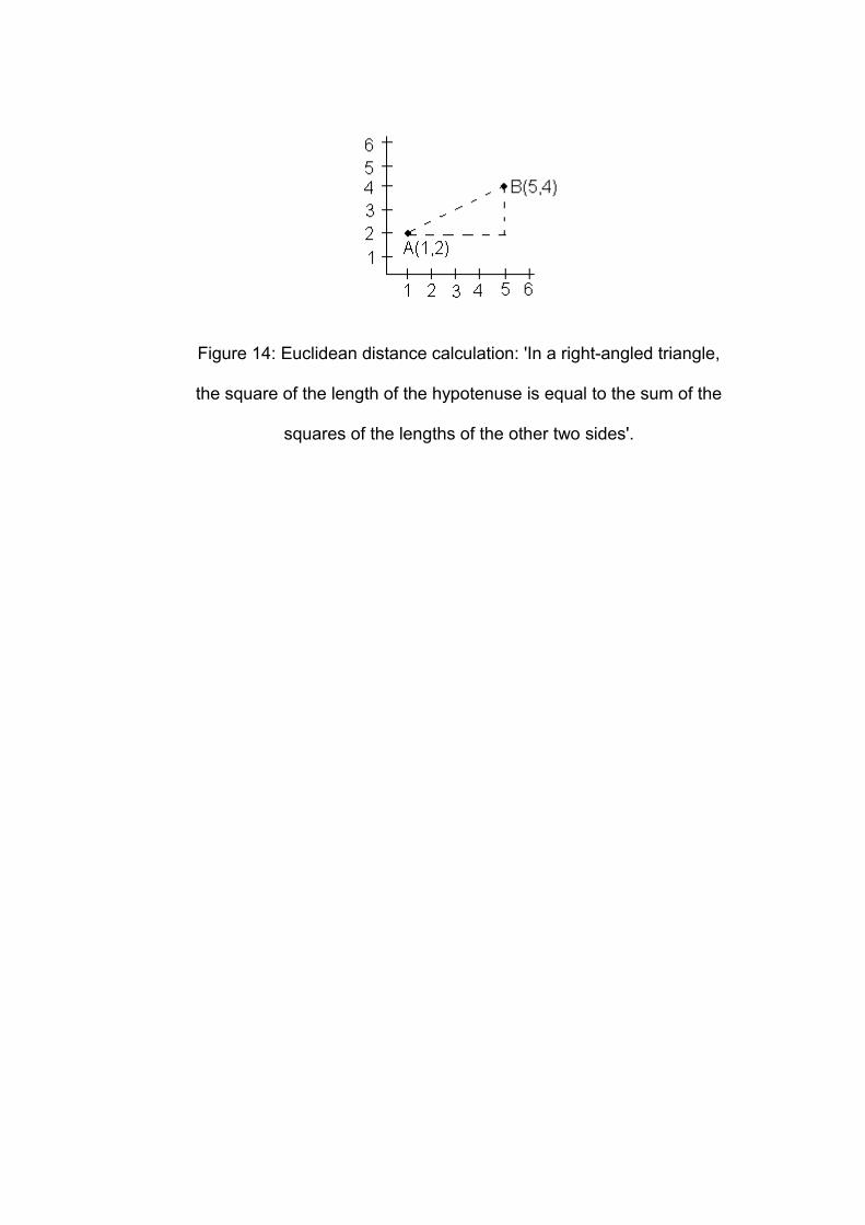
Figure 14: Euclidean distance calculation: 'In a right-angled triangle,

the square of the length of the hypotenuse is equal to the sum of the

squares of the lengths of the other two sides'.

v1 v2

1 27 46

2 29 48

3 30 50

4 32 51

5 34 54

6 55 9

7 56 9

8 60 10

9 63 11

10 64 11

11 78 72

12 79 74

13 80 70

14 84 73

15 85 69

16 27 55

17 29 56

18 30 54

19 33 51

20 34 56

21 55 13

22 56 15

23 60 13

24 63 12

25 64 10

26 84 72

27 85 74

28 77 70

29 76 73

30 76 69

a b

Figure 15: Hierarchical cluster analysis of two-dimensional data

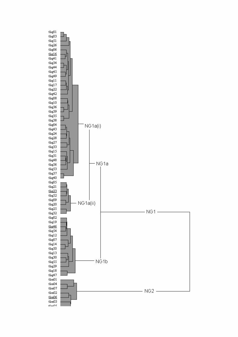
Figure 16: Hierarchical cluster analysis of the NECTE data matrix M

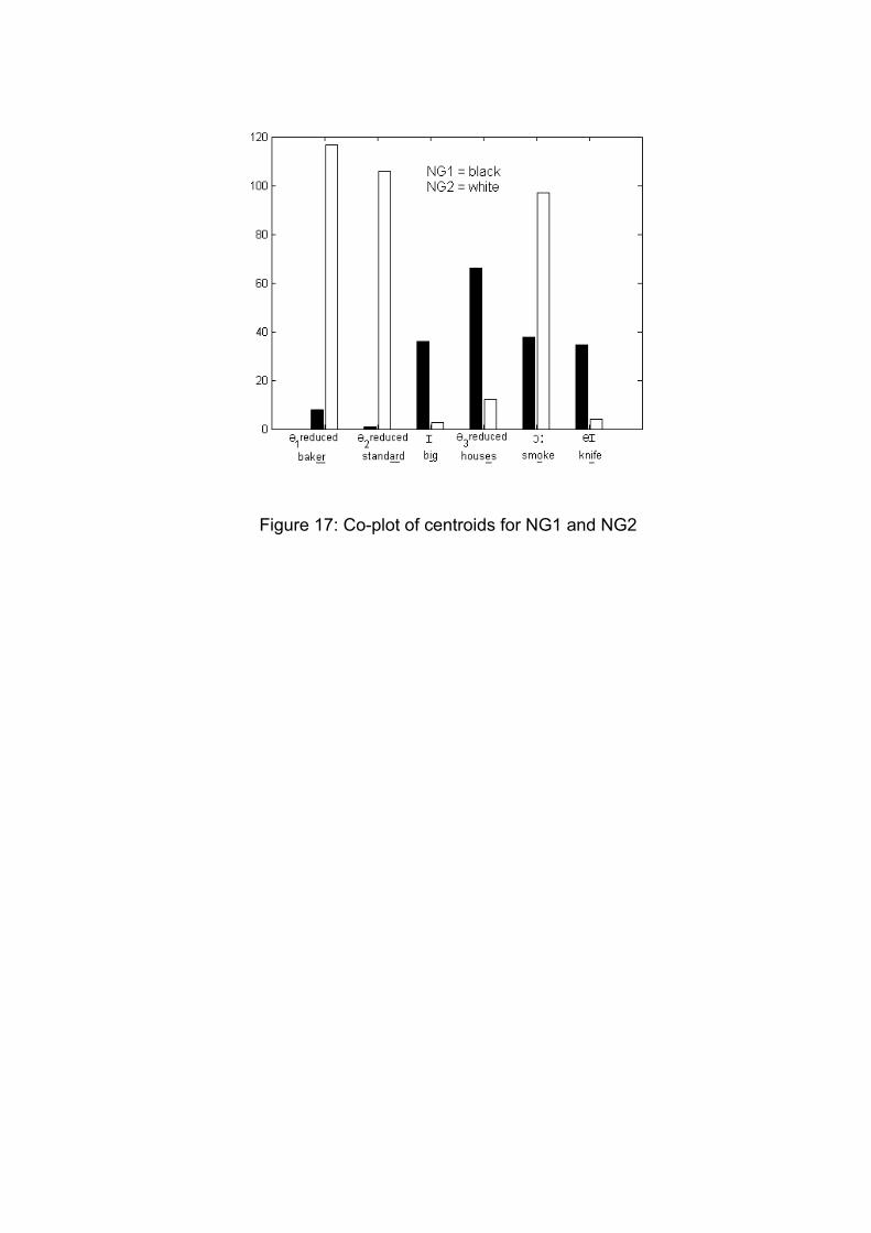
Figure 17: Co-plot of centroids for NG1 and NG2