USE OF PROBABILITY HYPOTHESIS DENSITY FILTER FOR ...

USE OF PROBABILITY HYPOTHESIS DENSITY FILTER FOR HUMANACTIVITY RECOGNITION

A THESIS SUBMITTED TOTHE GRADUATE SCHOOL OF NATURAL AND APPLIED SCIENCES

OFMIDDLE EAST TECHNICAL UNIVERSITY

BY

EL�F ERDEM GÜNAY

IN PARTIAL FULFILLMENT OF THE REQUIREMENTSFOR

THE DEGREE OF DOCTOR OF PHILOSOPHYIN

ELECTRICAL AND ELECTRONICS ENGINEERING

MARCH 2016

Approval of the thesis:

USE OF PROBABILITY HYPOTHESIS DENSITY FILTER FORHUMAN ACTIVITY RECOGNITION

submitted by EL�F ERDEMGÜNAY in partial ful�llment of the requirementsfor the degree of Doctor of Philosophy in Electrical and ElectronicsEngineering Department, Middle East Technical University by,

Prof. Dr. Gülbin Dural ÜnverDean, Graduate School of Natural and Applied Sciences

Prof. Dr. Gönül Turhan SayanHead of Department, Electrical and Electronics Eng.

Prof. Dr. Gözde Bozda§� AkarSupervisor, Electrical and Electronics Eng. Dept.,METU

Prof. Dr. Mübeccel DemireklerCo-supervisor, Electrical and Electronics Eng. Dept.,METU

Examining Committee Members:

Prof. Dr. Orhan Ar�kanElectrical and Electronics Eng. Dept., Bilkent University

Prof. Dr. Gözde Bozda§� AkarElectrical and Electronics Eng. Dept., METU

Prof. Dr. Ayd�n AlatanElectrical and Electronics Eng. Dept., METU

Assoc. Prof. Dr. Umut OrgunerElectrical and Electronics Eng. Dept., METU

Assist. Prof. Dr. Sevinç Figen ÖktemElectrical and Electronics Eng. Dept., METU

Date:

I hereby declare that all information in this document has been ob-tained and presented in accordance with academic rules and ethicalconduct. I also declare that, as required by these rules and conduct,I have fully cited and referenced all material and results that are notoriginal to this work.

Name, Last Name: EL�F ERDEM GÜNAY

Signature :

iv

ABSTRACT

USE OF PROBABILITY HYPOTHESIS DENSITY FILTER FOR HUMANACTIVITY RECOGNITION

GÜNAY, EL�F ERDEM

Ph.D., Department of Electrical and Electronics Engineering

Supervisor : Prof. Dr. Gözde Bozda§� Akar

Co-Supervisor : Prof. Dr. Mübeccel Demirekler

March 2016, 140 pages

This thesis addresses a Gaussian Mixture Probability Hypothesis Density (GM-

PHD) based probabilistic group tracking approach to human action recognition

problem. First of all, feature set of the video images denoted as observations are

obtained by applying Harris Corner Detector(HCD) technique following a GM-

PHD �lter, which is a state-of-the-art target tracking method. Discriminative

information is extracted from the output of the GM-PHD �lter and using these,

recognition features are constructed related to di�erent body segments and the

whole body. An unique Hidden Markov Model(HMM) belonging to each feature

is fed by these information and recognition is performed by selecting optimal

HMM's. The performance of the proposed approach is shown on the videos

in KTH Research Project Database and custom videos including occlusion sce-

narios.The results are presented as the percentage of the correctly recognized

videos. Same experiments on KTH database are performed for KLT tracker in-

stead of GMPHD in the proposed approach. In addition, a comparison is made

v

for an algorithm in the literature for the custom videos. The results shown that

proposed approach has comparable performance on KTH database and is better

in handling occlusion scenarios.

Keywords: Human action recognition, Gaussian Mixture PHD, Hidden Markov

Model, Harris Corner Detector

vi

ÖZ

�NSAN HAREKET ALGILAMA �Ç�N OLASILIKSAL H�POTEZYO�UNLUK F�LTRES� KULLANIMI

GÜNAY, EL�F ERDEM

Doktora, Elektrik ve Elektronik Mühendisli§i Bölümü

Tez Yöneticisi : Prof. Dr. Gözde Bozda§� Akar

Ortak Tez Yöneticisi : Prof. Dr. Mübeccel Demirekler

Mart 2016 , 140 sayfa

Bu tez, GMPHD tabanl� olas�l�ksal grup takibi ile insan hareketi alg�lama ko-

nusunu adreslemektedir. Önerilen çözüm, probleme s�ral� ve durumsal bir ³e-

kilde yakla³maya dayanmaktad�r. Öncelikle, Harris Corner Detector(HCD) tek-

ni§i kullan�larak video görüntülerindeki özellik setleri elde edilmektedir. Bunu

takiben elde edilen özellik kümeleri üzerinde son y�llarda popüler olan Gaussian

Mixture Probability Hypothesis Density (GMPHD) �ltresi uygulanmaktad�r.

GMPHD �ltresi ç�kt�s�ndan farkl�l�k yaratan bilgiler ç�kar�lmakta ve bu bilgiler

ile hem insan vücudunun farkl� bölümleri ile ili³kili hem de tüm vücudu temsil

eden alg�lama özellikleri ç�kar�lmaktad�r. Bu özellikler her bir özellik için olu³-

turulan Hidden Markov Modellerini(HMM) beslemekte ve optimal HMM'lerin

seçimi ile alg�lama sonucu olu³turulmaktad�r. Önerilen çözümün ba³ar�m� KTH

Ara³t�rma Projeleri Veri Taban� ve tez kapsam�nda çekilmi³ insan�n sabit bir ob-

jenin arkas�ndan geçti§i durumlardaki videolarda gösterilmi³ ve sonuçlar do§ru

vii

bir ³ekilde tan�mlanm�³ videolar�n yüzdesi olarak sunulmaktad�r. Ayn� deney-

ler KTH veritaban�nda, önerilen algoritman�n takip ad�m�nda KLT kullan�larak

da gerçekle³tirilmi³ ve tan�ma yüzdeleri ç�kar�lm�³t�r. Ayr�ca literatürde bulu-

nan yüksek performansl� bir algoritma ile bu videolar üzerinden kar³�la³t�rma

yap�lm�³t�r.

Anahtar Kelimeler: insan hareketi alg�lama, Gaussian Mixture PHD, Hidden

Markov Model, Harris Corner Detector

viii

To my beloved family...

ix

ACKNOWLEDGMENTS

I would like to thank my supervisor Professor Akar for his constant support,

guidance and friendship. It was a great honor to work with her for the last ten

years and our cooperation in�uenced my academical and world view highly. I

also would like to thank Prof. Demirekler for her strong support, guidance and

patience during all phases of this thesis study.

This thesis is also supported by my company ASELSAN by allowing me to focus

on my Ph.D. study and realizing the importance of combining the real world

engineering problems with the academic approaches, in an appropriate way.

My parents also has provided invaluable support for this work. I would like to

thank specially to my mother Gülbeyaz for her life-energy and my Father Mümin

for his humility and simplicity who always make me feel loved and cared. I also

want to thank to my mother-in law Vildan and my father-in law Mehmet for

their generosity, love and equanimity.

Last words goes to my priceless nuclear family. My �rst thanks go to my husband

Melih. You always make me feel special and loved, you are my life partner.

Secondly, I would like to thank to my beauty Ada. She is my �ower of love and

life energy. I also would like to thank to my little baby. You and Ada are the

source of my happiness and meaning of life. Me and your father do our best in

order to raise you as your own. I wish you a happy life my dears. This thesis

would not appear in this way without their endless love...

x

TABLE OF CONTENTS

ABSTRACT . . . . . . . . . . . . . . . . . . . . . . . . . . . . . . . . . v

ÖZ . . . . . . . . . . . . . . . . . . . . . . . . . . . . . . . . . . . . . . . vii

ACKNOWLEDGMENTS . . . . . . . . . . . . . . . . . . . . . . . . . . x

TABLE OF CONTENTS . . . . . . . . . . . . . . . . . . . . . . . . . . xi

LIST OF TABLES . . . . . . . . . . . . . . . . . . . . . . . . . . . . . . xv

LIST OF FIGURES . . . . . . . . . . . . . . . . . . . . . . . . . . . . . xvii

LIST OF ABBREVIATIONS . . . . . . . . . . . . . . . . . . . . . . . . xx

CHAPTERS

1 INTRODUCTION . . . . . . . . . . . . . . . . . . . . . . . . . 1

1.1 Introduction . . . . . . . . . . . . . . . . . . . . . . . . 1

1.2 Problem De�nition-Overview . . . . . . . . . . . . . . . 3

1.3 Problem Solution-Overview . . . . . . . . . . . . . . . . 4

1.4 Performance Comparison . . . . . . . . . . . . . . . . . 8

2 BACKGROUND . . . . . . . . . . . . . . . . . . . . . . . . . . 9

2.1 Harris Corner Detector . . . . . . . . . . . . . . . . . . 10

2.2 PHD Filter and Its Gaussian Mixture Implementation . 11

xi

2.3 Hidden Markov Models . . . . . . . . . . . . . . . . . . 14

3 LITERATURE SURVEY . . . . . . . . . . . . . . . . . . . . . . 23

3.1 Review on Human Action Recognition . . . . . . . . . . 24

3.2 Review on Hidden Markov Models . . . . . . . . . . . . 37

4 TRACKING . . . . . . . . . . . . . . . . . . . . . . . . . . . . . 41

4.1 Probabilistic Approaches . . . . . . . . . . . . . . . . . 42

4.1.1 Classical Probabilistic Approaches . . . . . . . 43

4.1.2 Particle Swarm Optimization Techniques withParticle Filter . . . . . . . . . . . . . . . . . . 47

4.1.3 Finite Set Statistics . . . . . . . . . . . . . . . 51

4.2 Deterministic Tracking . . . . . . . . . . . . . . . . . . . 53

4.2.1 Feature/Template Matching Techniques . . . . 53

4.2.2 Mean Shift Tracker . . . . . . . . . . . . . . . 57

5 PROPOSED ACTION RECOGNITION APPROACHUSINGGM-PHD AND HMM . . . . . . . . . . . . . . . . . . . . . . . . . . 59

5.1 Observation Extraction by Harris Corner Detector . . . 60

5.2 Group Tracking by GM-PHD . . . . . . . . . . . . . . . 61

5.2.1 Utilizing Image Intensity Di�erence in GM-PHD 64

5.3 Rotation of Action Direction . . . . . . . . . . . . . . . 65

5.4 High Level Recognition by Global Motion Analysis . . . 66

5.4.1 Determination of the Threshold Value . . . . . 67

5.4.2 Selection of the Group . . . . . . . . . . . . . . 69

xii

5.5 Determination of Discriminative Modes of GM-PHD . . 70

5.5.1 Group-1 . . . . . . . . . . . . . . . . . . . . . 70

5.5.2 Group-2 . . . . . . . . . . . . . . . . . . . . . 72

5.6 Clustering . . . . . . . . . . . . . . . . . . . . . . . . . . 73

5.6.1 Determination of Upper and Lower parts forGR-1 and GR-2 . . . . . . . . . . . . . . . . . 73

5.6.2 Determination of Upper-Left and Lower-Left partsfor GR-2 . . . . . . . . . . . . . . . . . . . . . 74

5.7 Construction of HMM Structure . . . . . . . . . . . . . 74

5.7.1 HMM Structure . . . . . . . . . . . . . . . . . 76

5.7.2 Construction of HMM Feature Set . . . . . . . 81

5.7.2.1 Mean and Standard Deviation of Po-sition . . . . . . . . . . . . . . . . . 82

5.7.2.2 Mean and Standard Deviation of Speed 83

5.7.2.3 Mean and Standard Deviation of An-gle . . . . . . . . . . . . . . . . . . 87

5.7.2.4 GM-PHD Distance . . . . . . . . . 89

5.7.2.5 Optimal SubPattern Assignment (OSPA)Metric . . . . . . . . . . . . . . . . 91

6 PERFORMANCE EVALUATION OF THE PROPOSED AP-PROACH . . . . . . . . . . . . . . . . . . . . . . . . . . . . . . 93

6.1 KTH Database . . . . . . . . . . . . . . . . . . . . . . . 93

6.2 Custom Occlusion Videos . . . . . . . . . . . . . . . . . 96

6.3 Experimental Results on KTH Database . . . . . . . . . 98

xiii

6.3.1 Experimental Parameters . . . . . . . . . . . . 98

6.3.2 Selection of Training Elements . . . . . . . . . 105

6.3.3 Experimented Approaches and Their Performances109

6.3.4 The E�ect of OSPA Parameter on the Perfor-mance . . . . . . . . . . . . . . . . . . . . . . . 111

6.3.5 Discussions . . . . . . . . . . . . . . . . . . . . 113

6.3.6 Discussion of the Algorithm for Misclassi�ed Videos115

6.4 Comparison between KLT and GMPHD . . . . . . . . . 117

6.5 Comparison with Literature . . . . . . . . . . . . . . . . 119

6.6 Discussion . . . . . . . . . . . . . . . . . . . . . . . . . 122

7 CONCLUSION . . . . . . . . . . . . . . . . . . . . . . . . . . . 123

REFERENCES . . . . . . . . . . . . . . . . . . . . . . . . . . . . . . . . 127

APPENDICES

A APPENDIX CHAPTER . . . . . . . . . . . . . . . . . . . . . . 135

CURRICULUM VITAE . . . . . . . . . . . . . . . . . . . . . . . . . . . 139

xiv

LIST OF TABLES

TABLES

Table 5.1 HCD Parameters Selected for the Algorithm. . . . . . . . . . 62

Table 5.2 GM-PHD outputs used as a basis for HMM . . . . . . . . . . 75

Table 5.3 Feature parameter vector for HMM . . . . . . . . . . . . . . . 76

Table 5.4 Group-1 : Running, Walking and Jogging action properties . . 77

Table 5.5 Group-2 : Boxing, Hand-Clapping and Hand-Waving action

properties . . . . . . . . . . . . . . . . . . . . . . . . . . . . . . . . 77

Table 5.6 HMM properties . . . . . . . . . . . . . . . . . . . . . . . . . 81

Table 6.1 De�ned Groups in the Context of the Thesis . . . . . . . . . . 95

Table 6.2 Frame Number for the Groups . . . . . . . . . . . . . . . . . . 98

Table 6.3 Selections of Windowing Type . . . . . . . . . . . . . . . . . . 98

Table 6.4 Selections of HMM Type . . . . . . . . . . . . . . . . . . . . . 102

Table 6.5 Group-1 Training Elements . . . . . . . . . . . . . . . . . . . 106

Table 6.6 Group-2 Training Elements . . . . . . . . . . . . . . . . . . . 107

Table 6.7 Methods and Performances for Group-1 . . . . . . . . . . . . 109

Table 6.8 Feature Vector Selection for Maximum Throughput for Group-1 110

Table 6.9 Methods and Performances for Group-2 . . . . . . . . . . . . 110

xv

Table 6.10 Feature Vector Selection for Maximum Throughput for Group-2 111

Table 6.11 Confusion Matrix for Windowing Type:1 and HMM Type:0 . 111









Table 6.20 GMPHD Results for the Feature Sets Including and not Includ-

ing OSPA Distance . . . . . . . . . . . . . . . . . . . . . . . . . . . 114

Table 6.21 KLT Results for the Feature Sets Including and not including

OSPA Distance . . . . . . . . . . . . . . . . . . . . . . . . . . . . . 118

Table 6.22 Performances of Tracklet and the Proposed Methods for the

Occlusion Scenarios ('W' stands for Walking action) . . . . . . . . . 121

Table A.1 GMPHD �lter (Prediction of birth targets, prediction of exist-

ing targets, construction of PHD update components steps),(adopted

from [67]). . . . . . . . . . . . . . . . . . . . . . . . . . . . . . . . . 136

Table A.2 GMPHD �lter (Measurement update and outputting steps),

(adopted from [67]). . . . . . . . . . . . . . . . . . . . . . . . . . . 137

Table A.3 GMPHD �lter (Pruning step), (adopted from [67]). . . . . . . 138

Table A.4 GMPHD �lter (Multitarget state extraction), (adopted from

[67]). . . . . . . . . . . . . . . . . . . . . . . . . . . . . . . . . . . . 138

xvi

LIST OF FIGURES

FIGURES

Figure 1.1 Training Flow of the Proposed Algorithm . . . . . . . . . . . 6

Figure 1.2 Testing Flow of the Proposed Algorithm . . . . . . . . . . . . 7

Figure 2.1 High Level Process Flow for the GMPHD �lter . . . . . . . . 14

Figure 3.1 Problem and Solution Domain of HAR [1] . . . . . . . . . . . 25

Figure 3.2 Cuboid Feautes of [13] . . . . . . . . . . . . . . . . . . . . . 27

Figure 3.3 Examples of clouds of interest points at di�erent scales [6] . . 28

Figure 3.4 Visualization of cuboid based behavior recognition [6] . . . . 29

Figure 3.5 Visualization of Features of [58] . . . . . . . . . . . . . . . . 30

Figure 3.6 Flow-chart of [6] . . . . . . . . . . . . . . . . . . . . . . . . . 31

Figure 3.7 An example of computing the shape-motion descriptor of a

gesture frame with a dynamic background. (a) Raw optical �ow �eld,

(b) Compensated optical �ow �eld, (c) Combined, partbased appear-

ance likelihood map, (d) Motion descriptor Dm computed from the

raw optical �ow �eld, (e) Motion descriptor Dm computed from the

compensated optical �ow �eld, (f) Shape descriptor Ds. [36] . . . . . 33

xvii

Figure 3.8 An example of learning. (a)(b) Visualization of shape and

motion components of learned prototypes for k = 16. (c) The learned

binary prototype tree. Leaf nodes, represented as yellow ellipses, are

prototypes. [36] . . . . . . . . . . . . . . . . . . . . . . . . . . . . . 34

Figure 3.9 Automatically extracted key poses and the motion energy chart

of three action sequences[40] . . . . . . . . . . . . . . . . . . . . . . 35

Figure 3.10 Action graph models. (a) The general model of a single action;

(b) Back-link (in red); (c) Inter-link (in blue); (d) A simple Action

Net consisting of the three actions. Each node contains a keypose

which is the the 2D representation of one view of an example 3D pose

as given in Figure 3.9 (e) The unrolled version of (d). Only models

with the �rst two pan angles are shown.[40] . . . . . . . . . . . . . . 36

Figure 3.11 A simple histogram to extract feature vectors from frames.[73] 37

Figure 4.1 Selected Solution Domain of the Thesis for the Tracking Problem 42

Figure 4.2 Explicit/Contour and Implicit/ Grid Representations of Sil-

houette [42] . . . . . . . . . . . . . . . . . . . . . . . . . . . . . . . 45

Figure 4.3 Some Results of Condensation Approach, [25] . . . . . . . . . 46

Figure 4.4 Convergence Criteria for Sequential Particle Swarm Optimiza-

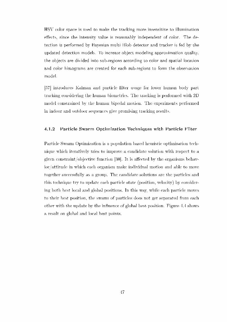
tion, [3] . . . . . . . . . . . . . . . . . . . . . . . . . . . . . . . . . . 48

Figure 4.5 Comparisons between variants of PF and sequential PSO, [3] 50

Figure 4.6 Experimental Results on Single Object Human Tracking, [74] 51

Figure 4.7 Structure of applied algorithms for comparison between KLT

and GMPHD . . . . . . . . . . . . . . . . . . . . . . . . . . . . . . . 57

Figure 4.8 A Mean Shift Tracker Result, [2] . . . . . . . . . . . . . . . . 58

Figure 5.1 Histogram of transformed X-Velocity state of GM-PHD . . . 69

xviii

Figure 5.2 HMM Frame for each feature of each action . . . . . . . . . . 79

Figure 5.3 Recognition by HMM . . . . . . . . . . . . . . . . . . . . . . 80

Figure 5.4 Histogram of Height of person in action in KTH database. . . 85

Figure 5.5 Histogram of Speed of person in action in KTH database. . . 86

Figure 5.6 Histogram Speed vs Velocity Angle of GR-1 actions . . . . . 88

Figure 5.7 Histogram Velocity Angle of GR-1 actions . . . . . . . . . . . 89

Figure 6.1 Example frames of each video in KTH Database . . . . . . . 95

Figure 6.2 Frames from the Tree Occlusion Test Videos . . . . . . . . . 97

Figure 6.3 Frames from the Person Occlusion Test Videos . . . . . . . . 97

Figure 6.4 Windowing Operations in Flow Chart . . . . . . . . . . . . . 100

Figure 6.5 Structure of Windowing Method-2 . . . . . . . . . . . . . . 101

Figure 6.6 Structure of Windowing Method-3 . . . . . . . . . . . . . . 102

Figure 6.7 Type-0: Fully Connected HMM State Flow . . . . . . . . . . 103

Figure 6.8 Type-1: Forward Connected HMM State Flow . . . . . . . . 104

Figure 6.9 Type-2: Half Connected HMM State Flow . . . . . . . . . . 105

Figure 6.10 An Individual HMM structure . . . . . . . . . . . . . . . . . 108

xix

LIST OF ABBREVIATIONS

AHMM Abstract Hidden Markov Model

AMI Accumulated Motion Image

CCA Canonical Correlation Analysis

CHSMM Coupled Hidden Semi-Markov Model

DBN Dynamic Bayesian Networks

FISST Finite Set Statistics

GEI Gait Energy Image

GMPHD Gaussian Mixture Probability Hypothesis Density

GR-1 Group-1

GR-2 Group-2

HAR Human Action Recognition

HCD Harris Corner Detection

HHMM Hierarchical Hidden Markov Model

HMM Hidden Markov Model

HoF Histogram of Optical Flow

HoG Histogram of Gradient

HLR High Level Recognition

HSMM Hidden Semi-Markov Model

JPDA Joint Probabilistic Data Association

KF Kalman Filter

KLT Kanade-Lucas-Tomasi

LP Lower Part

MBH Motion Boundary Histogram

MHT Multiple Hypothesis Tracking

MIL Multiple Instance Learning

NNC Nearest Neighborhood Classi�cation

PF Particle Filter

PCA Principle Component Analysis

xx

PDA Probabilistic Data Association

PHD Probability Hypothesis Density

PMHT Probabilistic Multiple Hypothesis Tracking

RFS Random Finite Sets

SVM Support Vector Machine

UL Upper Left

UP Upper Part

UR Upper Right

xxi

CHAPTER 1

INTRODUCTION

1.1 Introduction

Human Action Recognition (HAR) is a complex problem which requires individ-

ual solutions to detection, tracking and recognition sub-problems. This thesis is

an initial work showing the usability of GMPHD �lter for tracking phase in HAR

problems. This �lter is a promising tool for multi-target tracking problems and

is capable of group tracking when the number of targets in the scene is changing

as in the occlusion case. In the detection step, features are extracted by Harris

Corner Detector and then tracked by GMPHD �ltering technique as a group,

which is a state-of-the-art multi-target tracker. Afterwards, we utilize patterns

extracted from GMPHD �lter intensity and use these patterns to recognize the

actions by utilizing Hidden Markov Models (HMM).

In the literature, there is no existing solution which utilizes GMPHD �lter for

human motion analysis.The underlying idea is that if the body in the scene

is represented by the composition of multiple identical type features, the �lter

can handle the varying number of features and can group track all the features

instantaneously.

In video application problems, number of features is very likely to change for

each frame because of the following parameters:

• articulated parts of the body such as arms and legs resulting in occlusion

of the features,

1

• change in the background scene and

• dynamic noise in the scene

GM-PHD �lter is able to continuously track the occluded features for a certain

period of time by its inner mechanism which make it faster to include occlusion

to group tracking. Birth mechanism also helps capture new measurements to

group tracking in a short period of time.

Apart from the change of the number of features in the video sequence, GM-

PHD �lter performs the association and tracking at the same level which severely

reduces the computation and the complexity of the solution.

By applying GM-PHD �lter to a video sequence, 2D image information is con-

verted to a 3D intensity function which is a Gaussian Mixture. In this domain,

�rst two dimensions correspond to the positional information while 3rd dimen-

sion can be taken as the weights of the Gaussians in the mixture. Note that the

sum of weights corresponds to expected number of features in the scene. States

of GM-PHD includes information about position and velocity and represents the

dynamical behavior of the body parts like torso, arms, legs and head. To be

able to track the human body, all these articulated and non-articulated parts

should be tracked individually. In this thesis, GM-PHD constant velocity mo-

tion model is considered. Since there are di�erent types of action with di�erent

motion characteristics like sinusoidal as in walking or linear as in handclapping,

linear constant velocity is assumed to be the common subset of these motions.

As stated in chapter 3, proposed solutions for human activity recognition covers

several di�erent image processing techniques and evaluated on several di�erent

image databases. These studies generally focuses on extracting the information

from the image intensity and individual tracks of these features in time. These

solutions declares quite well performances up to the correct recognition of 95%

of the videos in the related databases as given in [1] and in section 3.

In this thesis, our aim is to model the human body parts as multiple-targets

and apply GM-PHD �lter, a multi-target tracker, to this problem. As another

novelty, we utilize image intensity information to guide GM-PHD �lter in which

2

di�erence between the image patches around the measurement is utilized in

weight determination of GM-PHD. The features are extracted from the image

intensities as the measurements to the tracker, yet the recognition step is based

only on the output of the multi-target GM-PHD tracker. The recognition pa-

rameters are extracted from the Gaussian Mixture intensity function belonging

to the whole body and di�erent parts of the body, as well. The recognition

phase, including both learning and testing, is based on the HMM technique and

the recognition parameters are certainly translated to the language of an HMM

structure. Explanations of these parameters and required pre-processing steps

are provided chapter 6.

1.2 Problem De�nition-Overview

The aim of the thesis is to identify the action taken by the human in a given

video sequence. The video set is selected as the KTH database described in [60],

which is a controlled database composed of videos of 25 individuals performing

6 di�erent action (walking, running, jogging, boxing, hand-clapping and hand-

waving) in 4 di�erent environments. Detailed information about the data base

is given in Chapter 6.

KTH database is chosen since it includes diverse environments when compared

to others. When the actions in the videos of KTH are analyzed, they seem to

have di�erent characteristics which bring di�culties to the recognition problem.

1. Di�erent aspects of the body (i.e., front, back and side pose)

2. Body with di�erent clothes and properties (i.e., gloves, topcoat, long

haired)

3. Zooming-in and out operations

4. Existence of Shadows in di�erent angles

5. Actions towards di�erent directions.

3

In order to eliminate these undesired e�ects on the recognition process, all the

information should be brought to a common reference. So the elimination of the

information belonging to the background scene but not the body itself should be

performed and mapping of the feature parameters to the reference point should

be done.

To speak speci�cally for each problem, if the aspect of the body is di�erent, then

the feature distribution of the body will be di�erent which a�ects recognition

problem signi�cantly. For this problem, we extract the height of the body in

action and normalize velocity related features using height information. But

considering side, front and back pose of the body, the di�erence in feature dis-

tribution is still a challenge for our problem. Besides, the individuals performing

action wear di�erent clothes. As examples, the person wearing topcoat and has

long hair a�ect the motion characteristics of the body signi�cantly, gloves cause

poor feature extraction at hand in darker background etc.

There is also zooming operation in the videos which causes;

1. Change in velocity information

2. Change in height

In order to decrease the negative e�ects of zooming, we normalize velocity vec-

tors using the height information of the body. But the virtual velocity in X and

Y direction still bring di�culty in recognition. In order to decrease the in�uence

of shadows, we decrease the number of features around shadows, but this oper-

ation decreases the number of features on the body. Considering the actions in

di�erence direction, we bring all motions to the same direction as given in 5.3.

The operations on the features because of not only video adversity but also for

recognition purposes are described in the following sections in detail.

1.3 Problem Solution-Overview

In this thesis, we intend to make recognition of human actions in a controlled

database using GM-PHD �lter output properties and propose a di�erent solution

4

to this problem. The �ow chart of the training and testing phases of the proposal

is given in Figure 1.1 and Figure 1.2, respectively.

2D image intensity contains information which does not only belong to body in

action but also to the background. So, as the �rst step, discriminative informa-

tion in the image has to be extracted. We used Harris Corner Detector technique

to extract features belonging to the body. The reason of selection of the Harris

Corner Detector as the feature extractor is its robustness and consistency and

suitability for multi-target tracking by extracting multiple corners in an image.

Group tracking is performed on the Harris corners by the GM-PHD �lter which

yields intensity function including the state information of each feature. After

elimination of outlier features using estimated set of states, they are re-calculated

with respect to the common reference scaling. Then parameters, that will be

used in the training phase, are calculated from GM-PHD intensity function. As

a �nal stage, an unique HMM structure for each action is built which are the

combination of HMMs belonging to each feature given in tables 6.5 and 6.6.

This implies each feature parameter has independent HMMs. After training

phase, the testing videos in the database are recognized by the trained HMM

structures and the recognition results are obtained by a voting algorithm in an

optimal way.

5

Figure 1.1: Training Flow of the Proposed Algorithm

6

Figure 1.2: Testing Flow of the Proposed Algorithm

7

1.4 Performance Comparison

The performance of the proposed algorithm is obtained by the videos in a con-

trolled database which gives a chance to compare with the existing algorithms.

The performance of the algorithm is about 89% and there are approaches with

higher performance results in the literature. In order to reveal the advantage of

GMPHD, we took custom videos including occlusion and compared the recogni-

tion performances of one of the most successful algorithm [54] and our approach.

We realize that our approach is more noise insensitive compared to the [54].

In addition we compared the group tracking performance of the GMPHD Filter

with tracking performance of KLT. This is performed by replacing GMPHD with

KLT tracker and evaluating the algorithm with the same parameter and video

sets. We see that our approach yields 10% more recognition performance than

the one with KLT.

8

CHAPTER 2

BACKGROUND

There are several representations of human body and corresponding tracking

methods in the literature. The most important parameter for solving the prob-

lem of action recognition is obviously the variety and number of information

types extracted from the video sequence. There are both deterministic and

probabilistic approaches utilized in HAR problem. Deterministic approaches di-

rectly uses the information extracted from the video sequence which does not

provide any information related to the statistics of the video. On the other hand

statistical approaches extracts and utilize the statistical information in the video

sequence. In this thesis both deterministic and statistical information is utilized

for action recognition purposes. Feature detection is performed in deterministic

ways whereas group tracking utilize the statistical information related to the

target dynamics and recognition is performed utilizing the statistical properties.

In HAR occlusion of the features is one of the major problems. It causes big

problems in deterministic approaches whereas the used group tracking method,

PHD �ltering, inherently deals with any type of occlusion within the �lter.

Apart from information related to the motion model of the features, PHD �lter-

ing reveals not only the information related to the motion characteristics ,i.e.,

position, velocity etc., but also the number of features at each frame.

In this thesis, we propose a complete algorithm which is capable of action recog-

nition in which features are extracted using Harris Corner Detector, group-

tracking of the features is performed with GM-PHD. The recognition is mainly

based on Hidden Markov Models and after extracting the desired information.

9

The algorithm is trained and tested by this technique.

Detailed information related to HCD, GM-PHD, and HMM will be provided in

this section for the sake of completeness. The novel approach based on these

techniques will be explained in Chapter 5.

2.1 Harris Corner Detector

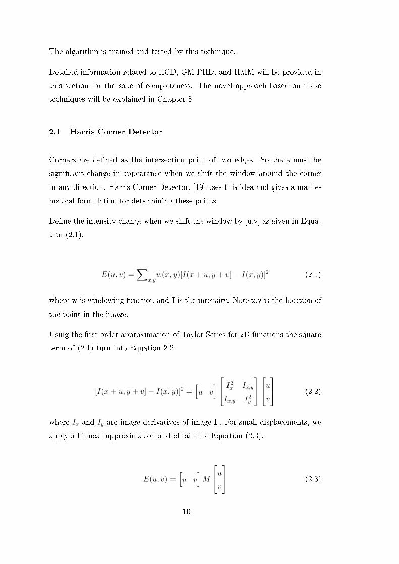
Corners are de�ned as the intersection point of two edges. So there must be

signi�cant change in appearance when we shift the window around the corner

in any direction. Harris Corner Detector, [19] uses this idea and gives a mathe-

matical formulation for determining these points.

De�ne the intensity change when we shift the window by [u,v] as given in Equa-

tion (2.1).

E(u, v) =∑

x,yw(x, y)[I(x+ u, y + v]− I(x, y)]2 (2.1)

where w is windowing function and I is the intensity. Note x,y is the location of

the point in the image.

Using the �rst order approximation of Taylor Series for 2D functions the square

term of (2.1) turn into Equation 2.2.

[I(x+ u, y + v]− I(x, y)]2 =[u v

] I2x Ix,y

Ix,y I2y

uv

(2.2)

where Ix and Iy are image derivatives of image I . For small displacements, we

apply a bilinear approximation and obtain the Equation (2.3).

E(u, v) =[u v

]M

uv

(2.3)

10

s

M =∑

x,yw(x, y)

I2x Ix,y

Ix,y I2y

(2.4)

Analyzing of M matrix gives us the corner points. First de�ne the measure of

corner response, R, as given in (2.5).

R = detM − k(trace(M))2 (2.5)

where

detM = λ1λ2 (2.6)

traceM = λ1 + λ2 (2.7)

where λ1 and λ2 are eigenvalues of M matrix. Note that k is an empirically

determined constant generally chosen between k = 0.04− 0.06

Corners are the points which have large R values which corresponds to the M

matrix with large and similar eigenvalues.

2.2 PHD Filter and Its Gaussian Mixture Implementation

In [17] and [44], the random set theory is de�ned as a theoretical framework

for multisensor-multitarget data processing in which a set of multiple targets at

time t is represented as a Random Finite Set (RFS). The Finite Set Statistics

(FISST) is the �rst systematic treatment of multisource-multitarget problem

which transforms the multisource-multitarget problem into a mathematically

equivalent single-sensor, single-target problem. The multitarget states and ob-

servations are represented as �nite sets instead of the vector notation. The

representation of the state of a target (commonly chosen as position and veloc-

ity) is represented by a state vector x, and the RFS is Xt = {x1, x2, .., xN(t)}where N(t) is variable target number at time t. Similarly, the measurement set

is Yt = {y1, y2, .., yM(t)} where M(t) is variable measurement number at time t.

11

The problem of FISST is its combinatorial complexity in the multi-target case.

Mahler proposed Probability Hypothesis Density (PHD) to approximate opti-

mal Bayes Filter and to reduce the complexity in [45]. The idea of PHD �ltering

is based on Finite Set Statistics (FISST) whose underlying idea is treating �nite

sets as random elements from probability theory point of view. In PHD frame-

work, the data obtained from various target/source is uni�ed under a single

Bayesian framework and all the detection, tracking and identi�cation problems

become a single problem.

In Human Tracking applications, two di�erent implementations of PHD �ltering

has been used. The particle �lter or the sequential Monte Carlo method is a

Monte Carlo simulation based recursive Bayes �lter and can be applied to solve

nonlinear and non-Gaussian problems. Other implementation which is called

Gaussian Mixture PHD (GM-PHD) is proposed for the linear, Gaussian target

dynamic model and birth process by [67] and it brings a closed form solution to

iterative calculation of means, covariance matrices and weights of the �lter.

In this section, further information for GM-PHD �lter is given for better under-

standing of the usage of the technique in the thesis solution.

Gaussian Mixture PHD (GMPHD) �lter brings forward a closed form solution

to the multiple target tracking problem. [67] explains the theory and pseudo-

code of this method yet the pseudo code of the algorithm is also given in the

appendix of the thesis (Section A).

Basic assumptions for the derivation of the �lter are:

• target dynamical model for a single target is linear Gaussian :

pk|k−1(z|x) = N (z;Ak−1x,Qk−1) (2.8)

• measurement model is also linear Gaussian:

py|x(y|x) = N (y;Ckx,Rk) (2.9)

12

• Target intensity, DXk(x), is in the form of a Gaussian mixture:

DXk(x) =

JXk∑i=1

w(i)

XkN (x;m

(i)

Xk, P

(i)

Xk) (2.10)

• Birth intensity, DBk(x), is also a Gaussian mixture:

DBk(x) =

JBk∑i=1

w(i)

BkN (x;m

(i)

Bk, P

(i)

Bk) (2.11)

Based on the assumptions above, predicted target intensity and measurement

updated target intensity are also found as Gaussian mixtures as in (2.12) and

(2.13), respectively.

DXk+1(x) =

JBk+1∑j=1

w(j)

Bk+1N (x;m

(j)

Bk+1, P

(j)

Bk+1) + pS

JXk∑i=1

w(i)

XkN (x; m

(i)

Xk, P

(i)

Xk) (2.12)

DXk+1(x) = (1− pD)

Jp∑j=1

w(j)p N (x;m(j)

p , P (j)p )+

Jp∑j=1

∑y∈Y

w(j)p q(j)(y)pD

DC(y) + pD∑Jp

i=1w(i)p q(j)(y)

N (x; m(j), P (j)) (2.13)

Note that pruning operation is required after obtaining the measurement up-

dated PHD to reduce the number of Gaussians to a certain level. After the

pruning phase, estimated positions of the targets are calculated by considering

the Gaussian mixture weights. Pseudo-code for pruning and state extraction

is given by the tables A.3 and A.4 in the appendix. Flow of the algorithm

implemented for the thesis is provided in Figure 2.1.

13

Figure 2.1: High Level Process Flow for the GMPHD �lter

2.3 Hidden Markov Models

Hidden Markov Model is a stochastic model which is a widely used probabilistic

framework in action recognition. HMMs and their extensions are well suited

for action recognition because of its sequential nature. They assume that the

underlying signal is of Markov Model which corresponds to that we can estimate

the next action from the current one and this is not far beyond our case when

we consider human actions visually.

In order to well suit the HMM model to the problem, fundamental model pa-

rameters have to be selected properly. The selection of number of hidden states

and both the model and number of observation symbols are three of these. In

learning phase of HMM, the values of the statistical parameters are determined

and in the testing phase the model giving the highest posterior probability is

taken as the action. In the next part, a background for HMM is given.

Theory of the Hidden Markov Model

HMM characterizes the statistical properties of the given signal which corre-

sponds to the sequences of feature values belonging to human body/action for

HAR case.

An HMM is characterized by the following parameters ([53]):

14

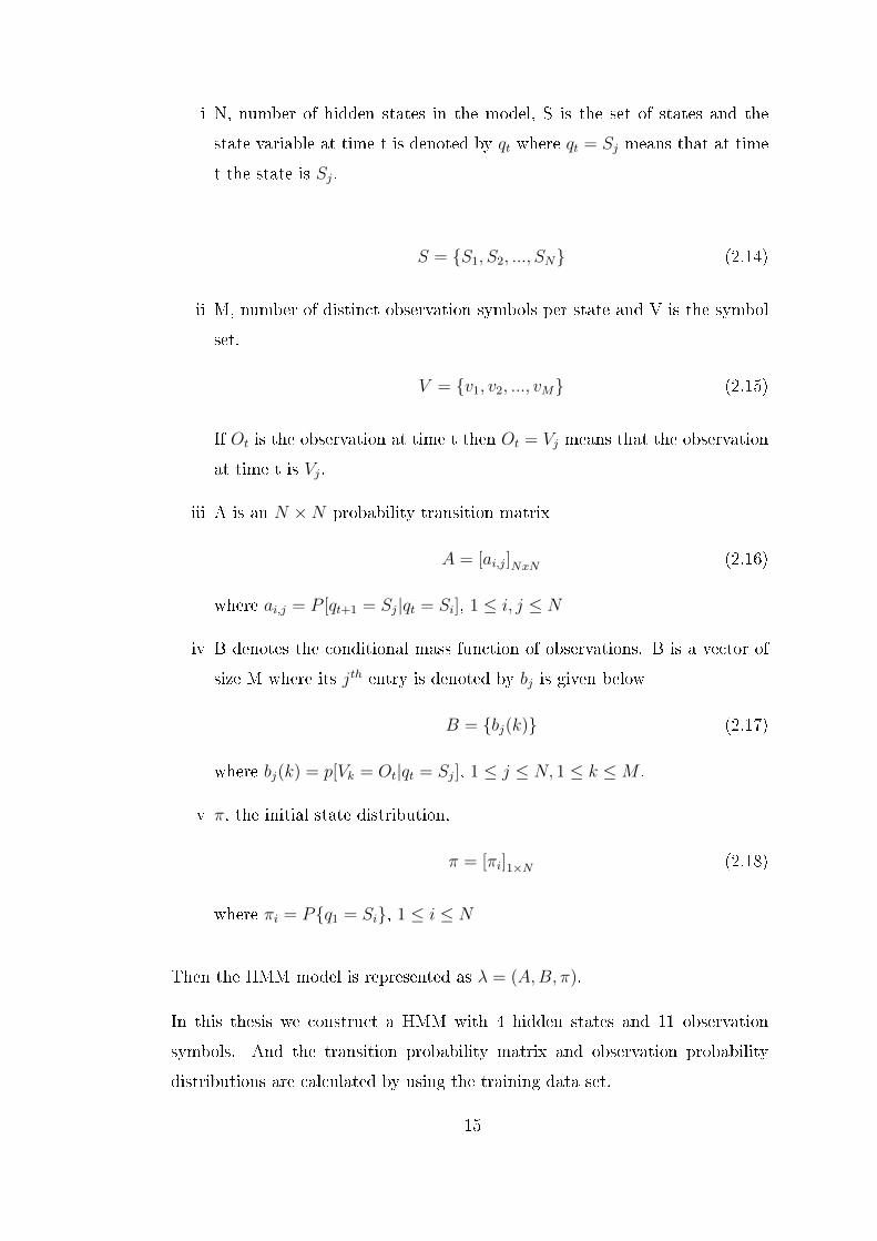
i N, number of hidden states in the model, S is the set of states and the

state variable at time t is denoted by qt where qt = Sj means that at time

t the state is Sj.

S = {S1, S2, ..., SN} (2.14)

ii M, number of distinct observation symbols per state and V is the symbol

set.

V = {v1, v2, ..., vM} (2.15)

If Ot is the observation at time t then Ot = Vj means that the observation

at time t is Vj.

iii A is an N ×N probability transition matrix

A = [ai,j]NxN (2.16)

where ai,j = P [qt+1 = Sj|qt = Si], 1 ≤ i, j ≤ N

iv B denotes the conditional mass function of observations. B is a vector of

size M where its jth entry is denoted by bj is given below

B = {bj(k)} (2.17)

where bj(k) = p[Vk = Ot|qt = Sj], 1 ≤ j ≤ N, 1 ≤ k ≤M .

v π, the initial state distribution,

π = [πi]1×N (2.18)

where πi = P{q1 = Si}, 1 ≤ i ≤ N

Then the HMM model is represented as λ = (A,B, π).

In this thesis we construct a HMM with 4 hidden states and 11 observation

symbols. And the transition probability matrix and observation probability

distributions are calculated by using the training data set.

15

Note that the observation symbols correspond to the physical output of the

system being modeled which are the quantized values of each feature given in

Table 6.5 and 6.6. Then, the observation symbols corresponds to the numbers

between 1 and 11.

There are three fundamental problems of HMM.

i Problem 1 : Evaluation Problem

The �rst problem is the evaluation problem, i.e., calculating the probability

that observed sequence is produced by the model. The solution of this

problem helps us classify the action in the testing phase.

ii Problem 2 : Decoding Problem

The second is decoding problem which calculated the most likely path of

the hidden states given the observation sequence.

iii Problem 3 : Problem of Adjusting Model Parameters (Learning)

The last problem is the calculation of the HMM parameters λ = (A,B, π)

by the training data.

Solution of Evaluation Problem Assume that the model λ = (A,B, π) and

observation sequence O1O2O3...Ot is given. The probability that this sequence is

produced by the model i.e., P (O|λ) is calculated by forward-backward procedure

e�ciently. First de�ne the forward variable, αt(i), that gives the probability of

the partial observation sequence until time t and hidden state is qt = Si.

αt(i) = P (O1O2O3..Ot, qt = Si|λ) (2.19)

αt(i) can be solved inductively with forward part of forward-backward procedure

2.22.

1. Initialization:

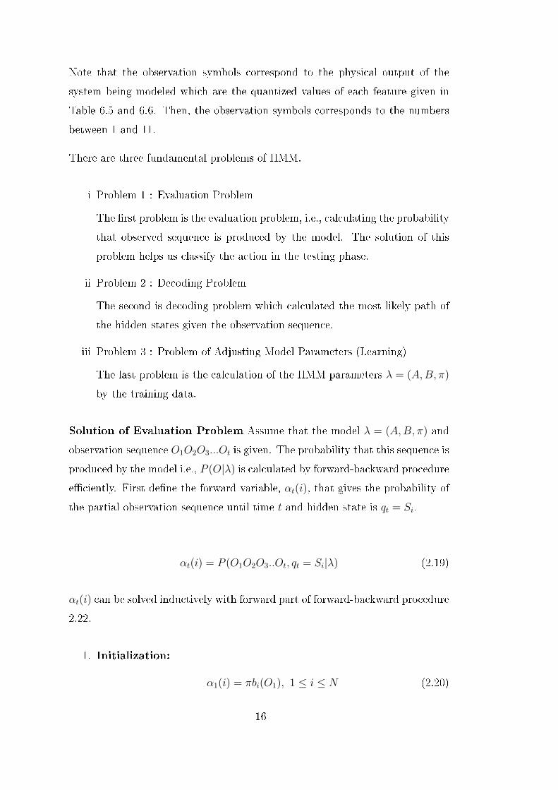
α1(i) = πbi(O1), 1 ≤ i ≤ N (2.20)

16

2. Induction:

αt+1(j) =

(N∑i=1

αt(i)aij

)bj(Ot+1), 1 ≤ t ≤ T − 1, 1 ≤ j ≤ N (2.21)

3. Termination:

P (O|λ) =N∑i=1

αT (i) (2.22)

In the initialization step, the forward probability is de�ned as the joint proba-

bility of state Si and the initial observation of O1. In induction step, Sj can be

reached at time t from N possible states. So summing over all the N possible

states Si and possible transitions aij at time t results in probability of Sj at

time t+ 1. Then αt+1(j) is calculated just by accounting for observation Ot+1 in

state j. In termination, summation over all terminal forward variables αT (i)is

performed.

In order give a complete solution backward recursion is presented here which is

indeed utilized in the solution of Problem 3.

The induction approach is very similar. First we de�ne a backward variable

βt(i) as the probability of the partial observation sequence from t+1 to the end.

βt(i) = P (Ot+1Ot+2Ot+3..OT , qt = Si|λ) (2.23)

The way of solving the backward variable, βt(i), is given in 2.26:

1. Initialization:

βT (i) = 1, 1 ≤ i ≤ N (2.24)

2. Induction:

17

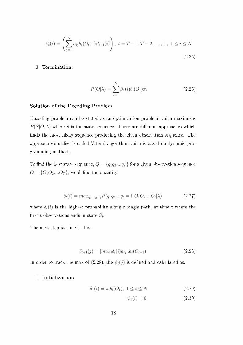
βt(i) =

(N∑j=1

aijbj(Ot+1)βt+1(i)

), t = T − 1, T − 2, . . . , 1 , 1 ≤ i ≤ N

(2.25)

3. Termination:

P (O|λ) =N∑i=1

β1(i)bi(O1)πi (2.26)

Solution of the Decoding Problem

Decoding problem can be stated as an optimization problem which maximizes

P (S|O, λ) where S is the state sequence. There are di�erent approaches which

�nds the most likely sequence producing the given observation sequence. The

approach we utilize is called Viterbi algorithm which is based on dynamic pro-

gramming method.

To �nd the best state sequence, Q = {q1q2....qT} for a given observation sequenceO = {O1O2....OT}, we de�ne the quantity

δt(i) = maxq1...qt−1P (q1q2....qt = i, O1O2....Ot|λ) (2.27)

where δt(i) is the highest probability along a single path, at time t where the

�rst t observations ends in state Si.

The next step at time t+1 is:

δt+1(j) = [maxiδt(i)aij].bj(Ot+1) (2.28)

In order to track the max of (2.28), the ψt(j) is de�ned and calculated as:

1. Initialization:

δ1(i) = πibi(O1), 1 ≤ i ≤ N (2.29)

ψ1(i) = 0. (2.30)

18

2. Recursion:

δt(j) = max1≤i≤N [δt−1(i)aij]bj(Ot), 2 ≤ t ≤ T, 1 ≤ j ≤ N (2.31)

ψt(j) = argmax1≤i≤N [δt−1(i)aij], 2 ≤ t ≤ T, 1 ≤ j ≤ N (2.32)

(2.33)

3. Termination:

P ∗ = max1≤i≤N [δt(i)] (2.34)

q∗T = argmax1≤i≤N [δt(i)]. (2.35)

4. Backtracking:

q∗t = ψt+1(q∗t+1), t = T − 1, T − 2, .., 1. (2.36)

Viterbi algorithm is very similar to forward step of evaluation problem but for

backtracking step. The maximization in (2.32) over previous steps which is used

in (2.21) is the fundamental di�erence.

Solution of Learning Problem

The most comprehensive and di�cult problem of HMM is to determine the

model parameters, λ = (A,B, π), given the data and the model. In fact, there is

no analytic and optimal way of estimating the model parameters. On the other

hand one can �nd λ = (A,B, π) which locally maximizes P (O|λ) in an itera-

tive manner. This is the Baum-Welch algorithm which is based on expectation

maximization:

First, let's de�ne the probability of being in state Si at time t and Sj at time

t+1 as follows:

ξt(i, j) = P (qt = Si, qt+1 = Sj|O, λ) (2.37)

19

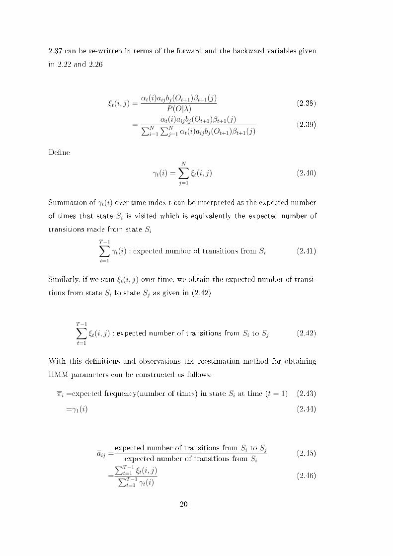
2.37 can be re-written in terms of the forward and the backward variables given

in 2.22 and 2.26

ξt(i, j) =αt(i)aijbj(Ot+1)βt+1(j)

P (O|λ)(2.38)

=αt(i)aijbj(Ot+1)βt+1(j)∑N

i=1

∑Nj=1 αt(i)aijbj(Ot+1)βt+1(j)

(2.39)

De�ne

γt(i) =N∑j=1

ξt(i, j) (2.40)

Summation of γt(i) over time index t can be interpreted as the expected number

of times that state Si is visited which is equivalently the expected number of

transitions made from state SiT−1∑t=1

γt(i) : expected number of transitions from Si (2.41)

Similarly, if we sum ξt(i, j) over time, we obtain the expected number of transi-

tions from state Si to state Sj as given in (2.42)

T−1∑t=1

ξt(i, j) : expected number of transitions from Si to Sj (2.42)

With this de�nitions and observations the reestimation method for obtaining

HMM parameters can be constructed as follows:

πi =expected frequency(number of times) in state Si at time (t = 1) (2.43)

=γ1(i) (2.44)

aij =expected number of transitions from Si to Sj

expected number of transitions from Si(2.45)

=

∑T−1t=1 ξt(i, j)∑T−1t=1 γt(i)

(2.46)

20

bj(k) =expected number of times in state j and observing symbol Vk

expected number of times in state j(2.47)

=

∑T−1t=1 γt(i)

s.t.Ot = Vk∑T−1t=1 γt(i)

(2.48)

The objective function that we maximize is as follows:

Q(λ, λ) =∑Q

P (Q|O, λ) logP (Q|O, λ) (2.49)

where Q is the state sequence.

The algorithm continues until �nding the best sequence of S1...Sk and goes to

model parameter estimation step.

It is known that Baum-Welch algorithm improves the value of the objective

function at each step and converges to a local optimal.

21

CHAPTER 3

LITERATURE SURVEY

Human Action Recognition from visual sources is a challenging and complex

problem for which there are several techniques proposed in the literature. The

challenge of the problem does not only come from the unexpected human behav-

ior, but also comes from the side e�ects caused by occlusion, moving background,

clutter, illumination, non-rigidity and loss of 3D information.

In the literature, there are several approaches for human action recognition from

visual resources. In this section, we mention about these approaches and make

a comparison to our approach.

To begin with, action recognition problem from visual resources have the fol-

lowing components: feature extraction, action learning and classi�cation, and

action recognition and segmentation [52]. In this work we divided the problem

into 3 major sub-problems which are feature extraction, tracking and recognition

of action where recognition includes learning and action recognition phases.

This paradigm heavily relies on the performance of the previous process. In

the feature extraction step, the discriminative and reproducible features have

to be selected since they a�ects performance of tracking. Besides, the accuracy

of tracking is very critical since the recognition step uses the outputs of the

tracking phase which is not reliable in a cluttered environment. There are several

expression of recognition methodologies using di�erent criteria discussed in 3.1.

In literature review section, the literature survey for each sub-problem and com-

parison to our approach is given in detail.

23

3.1 Review on Human Action Recognition

Human action recognition is an active with a wide range of research made and

a diverse �eld of real world applications such as surveillance, recognition of

abnormal behavior etc. From computer vision point of view, action recognition is

�nding the best matched pattern, which is obtained previously in training phase,

to the current observation. Here, the critical issue is the way of representing the

pattern and the way/approach of recognition.

Action recognition from visual sources with di�erent individuals brings di�-

culties due to variations in motion performance, recording settings and inter-

personal di�erence [52]. Another di�culty comes from the fact that recognition

is severely a�ected from the accuracy of tracking since it uses the tracking output

directly for recognition purposes.

There are single layer and multiple layer(hierarchical) approaches to human ac-

tion recognition problem [1]. Single layer approaches deal with single human

body and gesture recognition whereas hierarchical approaches are generally ap-

plied to more complex problems such as human interactions and group activity

cases. In this work, we are interested in recognition of single human body so

make a review of single layer approaches. There are various single layer ap-

proaches one of which utilizes 3D cumulative of image sequences (called space-

time) and the other uses the information between sequence of images (called

sequential) [1]. Figure 3.1 show the decomposition of human recognition ap-

proaches and show the solution domain of the thesis. In this work we handle

the recognition problem as a sequence of observations instead of 3D space time

volume which corresponds to a sequential approach.

24

Figure 3.1: Problem and Solution Domain of HAR [1]

In this part, the literature survey for single layer approaches are presented. Con-

sidering 3D space-time approaches, the extracted features may contain history

information. One of the approaches, [54] extracts tracklet descriptors. Firstly,

the features are extracted and tracked by means of KLT Feature Tracker. Then

the histogram of oriented gradients (HOG) and histogram of optical �ow (HOF)

properties of the tracked points on each trajectory are obtained and tracklet

descriptors for each trajectory longer than 3 frames is constructed. The method

utilized the bag of words technique and project the each tracklet to the closest

dictionary element. Then the SVM classi�cation is performed by histogram these

words. The approach has 94.5% recognition performance with leave-one-out

evaluation on KTH database. Note that, we utilize this method for benchmark-

ing in occlusion scenarios. Another approach,[22], uses motion history image

(MHI) and combined it with feature HoG which contains information on direc-

tions and magnitudes of edges and corners. The classi�cation is performed by

simulated annealing multiple instance learning support vector machine (SMILE-

SVM) to acquire a global optimum. This approach gives a 100% success in CMU

database.

Ziaeefar st al. [76] propose a Cumulative Skeletonized Image (CSI) which is

constructed by combining the skeleton centers along time in a polar coordinate.

The classi�cation is performed by analyzing this angular/distance histograms

and using hierarchical SVM.

25

Accumulated Motion Image (AMI) is proposed by [33] which is a spatio tem-

poral feature composed of average of image di�erences. The distance between

rank matrices of query and candidate videos are used for recognition purposes.

AMI concept is motivated by Gait Energy Image [18]. There are e�orts using

Canonical Correlation Analysis (CCA) as a measure between videos with 95.33

% performance [32] and Principle Component Analysis (PCA) to one cycle of

repetitive action in the video [37].

The approaches using space-time trajectories, one of which [68], extract dense

interest points and track them by displacement of information and obtain dense

trajectories of these points. They make use of HoG, Histogram of Optical Flow

(HoF) and propose Motion Boundary Histogram (MBH) as local descriptors

around the interest points as features. They make recognition by means of these

features and obtain 94.2 % performance on KTH database. The method of

[46] uses Harris3D interest points and extracts the feature trajectory using KLT

tracker. The trajectories are represented as sequences of log-polar quantized ve-

locities. The feature utilized in recognition is based on velocity history of tracked

points and performs recognition by means of utilizing a generative weighted mix-

ture model. This methods has a 74 % performance on KTH database.

The space-time local features are described as the descriptive points and their

surroundings in 3D volumetric data with unique discriminative characteristics.

They can be categorized as sparse and dense. The most popular sparse features

are 3D Harris Detector [35] and Dollar detector [13] where Figure 3.2 shows

the features of the latter which are obtained by Gaussian smoothing kernel

and Gabor �ltering. Methods using optical �ow are examples of the dense

case. Local features provides increased robustness to noise and pose variation

and it compares the cuboid features for SVM and nearest neighborhood (NNC)

classi�cation methods obtaining over 80 % performance in [13].

26

Figure 3.2: Cuboid Feautes of [13]

Studies in [28] and [6] improves performance of [13] by utilizing clouds of the

proposed interest points. [28] uses k-means to cluster the clouds and perform

classi�cation by proposed Asymmetric Bagging and Random Subspace Support

Vector Machine (ABRS-SVM) with a 95.3 % performance on KTH database. On

the other hand [6] uses clouds which are obtained at di�erent temporal scales

given in Figure 3.3.

27

Figure 3.3: Examples of clouds of interest points at di�erent scales [6]

The features proposed in [6] are given in Figure 3.4 with comparison to features

of [13] which uses local information within a small region and sensitive to video

noise and has low performance in zooming cases. The proposed features are

extracted by �rst taking frame di�erence for understanding of focus region, then

utilizes 2D Gabor �ltering on the detected regions of di�erent orientations which

identi�es salient features as given in Figure 3.4 and has 93.17 % performance on

KTH videos.

28

Figure 3.4: Visualization of cuboid based behavior recognition [6]

Harris3D [35] features are utilized in [63] in which classi�cation is made by PCA-

SVM and has 93.83 % performance on the KTH database. In order not to su�er

from sparsity, [16] uses dense 2D Harris corners in multiple scales with two scale

hierarchical grouping. In [58] 2D Harris Corners are extracted in each frame,

as in our case, and local features are de�ned on log-polar histograms by using

temporal similarities as given in Figure 3.5

29

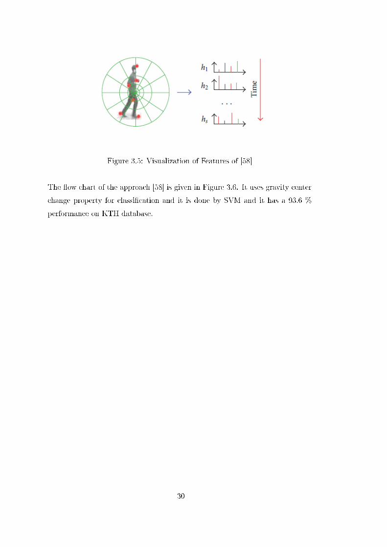
Figure 3.5: Visualization of Features of [58]

The �ow chart of the approach [58] is given in Figure 3.6. It uses gravity center

change property for classi�cation and it is done by SVM and it has a 93.6 %

performance on KTH database.

30

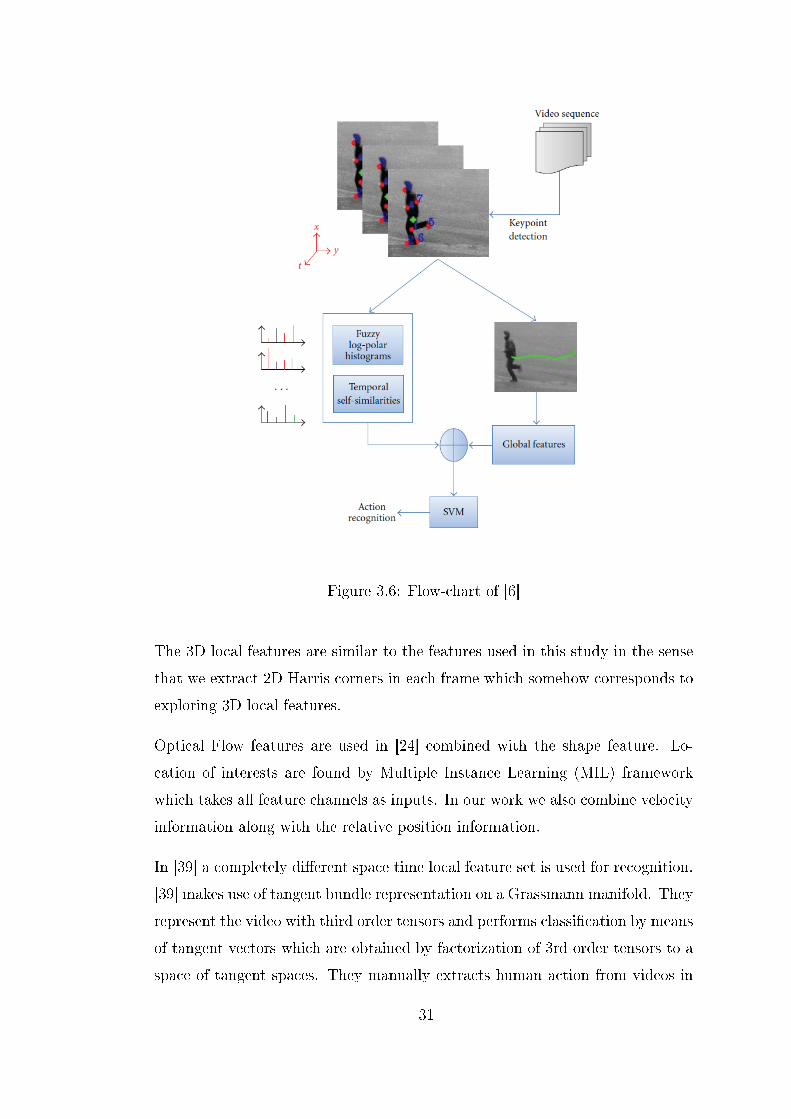
Figure 3.6: Flow-chart of [6]

The 3D local features are similar to the features used in this study in the sense

that we extract 2D Harris corners in each frame which somehow corresponds to

exploring 3D local features.

Optical Flow features are used in [24] combined with the shape feature. Lo-

cation of interests are found by Multiple Instance Learning (MIL) framework

which takes all feature channels as inputs. In our work we also combine velocity

information along with the relative position information.

In [39] a completely di�erent space time local feature set is used for recognition.

[39] makes use of tangent bundle representation on a Grassmann manifold. They

represent the video with third order tensors and performs classi�cation by means

of tangent vectors which are obtained by factorization of 3rd order tensors to a

space of tangent spaces. They manually extracts human action from videos in

31

KTH database and re-size the videos to 20× 20× 32 windows. Their approach

uses leave-one-out cross validation technique and achieves a 97 % success of

recognition in KTH database.

When we investigate the sequential approaches in Figure 3.1, in which the tem-

poral relationships of observations are extracted and used in recognition phase,

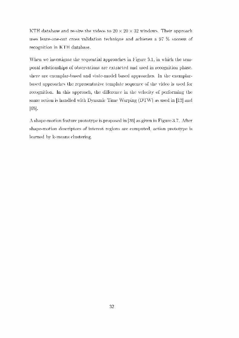
there are exemplar-based and state-model based approaches. In the exemplar-

based approaches the representative template sequence of the video is used for

recognition. In this approach, the di�erence in the velocity of performing the

same action is handled with Dynamic Time Warping (DTW) as used in [12] and

[65].

A shape-motion feature prototype is proposed in [36] as given in Figure 3.7. After

shape-motion descriptors of interest regions are computed, action prototype is

learned by k-means clustering.

32

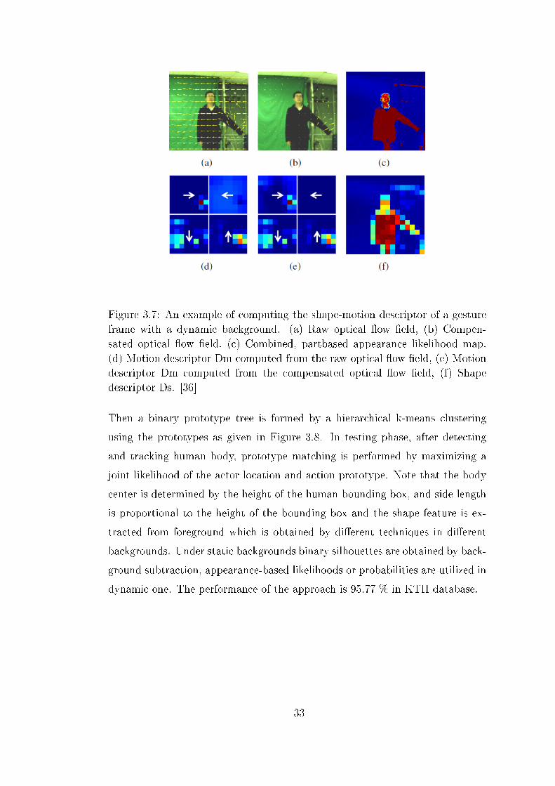
Figure 3.7: An example of computing the shape-motion descriptor of a gestureframe with a dynamic background. (a) Raw optical �ow �eld, (b) Compen-sated optical �ow �eld, (c) Combined, partbased appearance likelihood map,(d) Motion descriptor Dm computed from the raw optical �ow �eld, (e) Motiondescriptor Dm computed from the compensated optical �ow �eld, (f) Shapedescriptor Ds. [36]

Then a binary prototype tree is formed by a hierarchical k-means clustering

using the prototypes as given in Figure 3.8. In testing phase, after detecting

and tracking human body, prototype matching is performed by maximizing a

joint likelihood of the actor location and action prototype. Note that the body

center is determined by the height of the human bounding box, and side-length

is proportional to the height of the bounding box and the shape feature is ex-

tracted from foreground which is obtained by di�erent techniques in di�erent

backgrounds. Under static backgrounds binary silhouettes are obtained by back-

ground subtraction, appearance-based likelihoods or probabilities are utilized in

dynamic one. The performance of the approach is 95.77 % in KTH database.

33

Figure 3.8: An example of learning. (a)(b) Visualization of shape and motioncomponents of learned prototypes for k = 16. (c) The learned binary prototypetree. Leaf nodes, represented as yellow ellipses, are prototypes. [36]

Talking about state model-based approaches, general trend is to represent each

action by hidden states. In this area, utilization of HMM is very common as given

in [5] and [72]. One of the drawbacks of HMM is modeling the duration of action

and determining the transition matrix among this information.There are also

extension of HMM techniques proposed as Coupled Hidden Semi-Markov Model

(CHSMM) to overcome this problem and model duration of human activities

as given in [40] and [48]. Transition of the synthetic poses is represented by a

graph model called Action Net where each node contains a keypose which is the

the 2D representation of one view of an example 3D pose as given in Figure 3.9.

34

Figure 3.9: Automatically extracted key poses and the motion energy chart ofthree action sequences[40]

The HMM structure in [40] is given in Figure 3.10 where each node represents

one key pose and an action composes of a chain of the extracted keyposes.

35

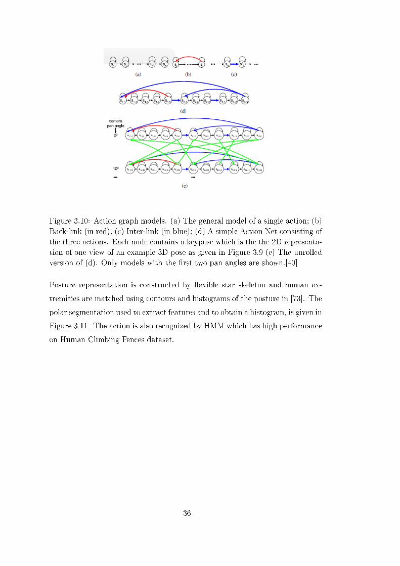
Figure 3.10: Action graph models. (a) The general model of a single action; (b)Back-link (in red); (c) Inter-link (in blue); (d) A simple Action Net consisting ofthe three actions. Each node contains a keypose which is the the 2D representa-tion of one view of an example 3D pose as given in Figure 3.9 (e) The unrolledversion of (d). Only models with the �rst two pan angles are shown.[40]

Posture representation is constructed by �exible star skeleton and human ex-

tremities are matched using contours and histograms of the posture in [73]. The

polar segmentation used to extract features and to obtain a histogram, is given in

Figure 3.11. The action is also recognized by HMM which has high performance

on Human Climbing Fences dataset.

36

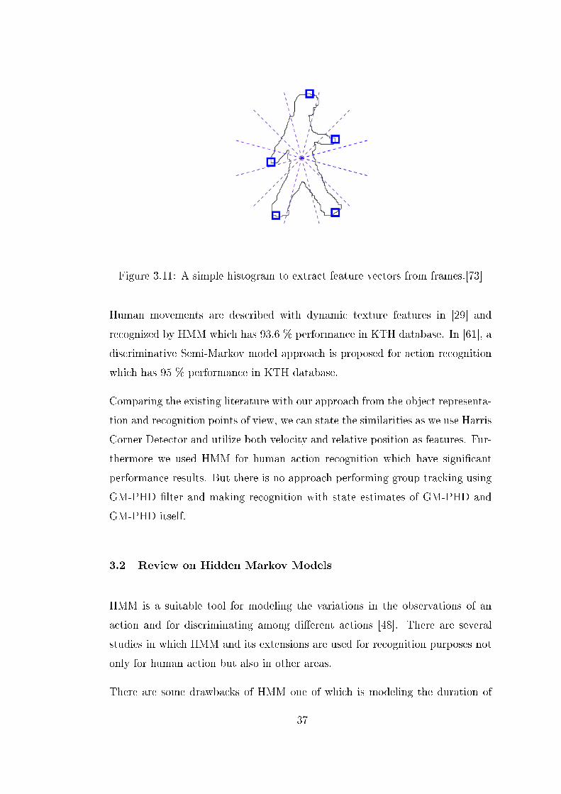
Figure 3.11: A simple histogram to extract feature vectors from frames.[73]

Human movements are described with dynamic texture features in [29] and

recognized by HMM which has 93.6 % performance in KTH database. In [61], a

discriminative Semi-Markov model approach is proposed for action recognition

which has 95 % performance in KTH database.

Comparing the existing literature with our approach from the object representa-

tion and recognition points of view, we can state the similarities as we use Harris

Corner Detector and utilize both velocity and relative position as features. Fur-

thermore we used HMM for human action recognition which have signi�cant

performance results. But there is no approach performing group tracking using

GM-PHD �lter and making recognition with state estimates of GM-PHD and

GM-PHD itself.

3.2 Review on Hidden Markov Models

HMM is a suitable tool for modeling the variations in the observations of an

action and for discriminating among di�erent actions [48]. There are several

studies in which HMM and its extensions are used for recognition purposes not

only for human action but also in other areas.

There are some drawbacks of HMM one of which is modeling the duration of

37

time. Besides decision of number of hidden states and observation symbols is

very problem dependent. When we investigate the learning problem, it �nds the

local maxima which is one of local maxima of a complex domain.

HMMs are basically a class of Dynamic Bayesian Networks (DBN) where there is

a temporal evolution of nodes. The elements of HMM and detailed background

information is given in Section 2.3. Hierarchical HMM (HHMM) is proposed for

the gap between low level data and high level semantics which utilizes HMM for

action recognition which models complex multi-scale structure in [8]. Abstract

HMM (AHMM) where each state is dependent to a hierarchy of actions is de-

scribed in [9]. In order to overcome the duration problem, Hidden Semi Markov

Model (HSMM) which has explicit state duration models is introduced and is

applied to video events in [21]. Switching Semi Markov Model (S-SHMM) is

proposed in [14] which is a two layer extension of HSMM and applied to recog-

nition.

There are many approaches proposed to improve the performance of HMM.

However, in this work we utilize standard HMM since we use quantized values

of features as observation symbols and has constant frame size for each group.

Focusing on the representation of observations shows that there many di�erent

code-book generation mechanisms. In [72], the code-book is generated by select-

ing 11 number of representative frames of the whole action. The ratio of white

pixels in 8× 8 regions are calculated and the sequence of these features is used

as the feature in symbol construction.

[66] utilizes 17 dimensional feature set for recognition purposes using HMM with

3 hidden states and 5 Gaussian Mixtures for each observation symbol. It also

extracts projection histogram features of vertical and horizontal axis which is

said to be su�cient in order to infer posture of the person and make a comparison

of the two feature sets in two databases. 17 dimensional feature set has higher

performance on Weizmann Data where the latter feature set is better in UT-

Tower data set.

The a�ect of code-book size, clustering methods (K-means vs LBG) and feature

38

selection on recognition performance is investigated in [64]. It is concluded that

the best performance is obtained with code book size greater than 30 in LGB

clustering with IC-based shape features using LDA. Note that in our case, we

selected the code book size as 11 which correspond to mapping all features into

the 0-10 interval.

39

CHAPTER 4

TRACKING

Tracking is simply a process which generates the trajectory of the object being

tracked. There are di�erent approaches to track human bodies in the video.

Tracking can be performed by detecting the possible objects in each frame

and establishing correspondence between the detected objects in the consec-

utive frames. Another approach is to make detection �rst, then updating the

track by estimating the new state of the object(its extracted parameters) in the

following frame iteratively.

The object states and the motion capabilities of the human are determined by

the object representation approach, so the tracking method is highly correlated

to the object representations type.

The tracking methods can be categorized into two: probabilistic and determin-

istic.In this thesis, we utilize a probabilistic technique for group tracking called

GMPHD which both group track the body as a complete object and constructs

state estimates of individual features/measurements for tracking purposes. So

an intensity map is obtained by a combination of Gaussian Mixtures belonging

to the measurements/features.

The solution domain utilized in this work is given in Figure 4.1.

41

Figure 4.1: Selected Solution Domain of the Thesis for the Tracking Problem

4.1 Probabilistic Approaches

There is unpreventable noise existence in visual tracking. The source of the

noise might be the visual sensor as well as the object behavior itself. In or-

der to take this in-suppressible noise into account, the probabilistic approaches

are utilized and some di�erent estimation techniques are used. In the case of

multiple target existence, in addition to these estimation techniques, di�erent

association techniques are proposed. In this part, brief information on these

techniques is provided. In probabilistic approaches, the most frequently chosen

object representation type for object tracking is the point representation. The

state of the object is often chosen as the location and velocity of the object and

tracking becomes the operation of �nding the most probable state in the next

frame (prediction) and update this prediction by the new observation (correc-

tion). In probabilistic approaches, as well as point representations, the shape

and counter information/representation is also common.

Probabilistic approaches can be categorized into three classes depending on how

the problem is modeled:

(i) Classical Probabilistic Approaches : Kalman based

42

(ii) Particle Swarm Optimization Techniques with Particle Filter

(iii) Random Set Statistics : Finite Set Statistics

4.1.1 Classical Probabilistic Approaches

To begin with the single target case, the most common approach is Kalman Filter

and its various versions. Brie�y speaking, Kalman Filter is a linear estimation

technique where the state variables are assumed to be Gaussian distributed.

The �rst step is the prediction step in which the prediction of the current state

is found from the target dynamics and previous information. Then as the new

measurement comes, the prediction is updated using the correction step. These

prediction and correction steps are coupled and performed iteratively for each

new incoming data. Kalman �lter has been a quite popular technique in vision

for a very long time [7].

Particle Filter Method is proposed to overcome the Gaussianality and the lin-

earity constraints of Kalman �ltering [34]. In particle �lter, the distribution

is approximated by the samples and these samples are taken into account in-

stead of the whole distribution. This approach breaks the Gaussian probability

distribution constraint of KF. The samples known as particles are Dirac-delta

functions and are weighted (with observation), predicted and corrected which is

similar to classical Kalman �lter in �tness.

Another classical statistical tracking approach is using some data association

techniques. Probabilistic Data Association (PDA) technique takes each potential

target as a track candidate and the statistical distribution of the track error

and clutter is used in this algorithm. This method considers only one of the

measurements as a track where all the others are taken as false alarms.

Considering Multiple target scenarios, there is a necessity to perform an asso-

ciation mechanism between the tracked objects and the measurements. After

extracting the association information, the single target approaches are safely

applied to each target. There are many association mechanisms for multiple

target case. For instance, Joint Probabilistic Data Association (JPDA) is an

43

extension of PDA that is capable of representing multiple targets by associating

all measurements with each track. [55] uses a version of this method for region

tracking. The disadvantage of this method is that it is not able to track when

the number of tracked objects changes in the scene.

Similarly, [47] models data association and probability of target/track presence

with a recursive probabilistic approach called integrated probabilistic data asso-

ciation (IPDA) which is said to have less computational complexity with almost

the same tracking performance with PDA [31]. Multiple Hypothesis Tracking

(MHT), proposed by [56], is another association algorithm which is capable of

handling the change in the number of objects in the scene. MHT considers

all possible association hypothesis so in a few iterations the number of possi-

ble tracks become computationally untractable. There is another probabilistic

approach, called Probabilistic Multiple Hypothesis Tracking (PMHT), proposed

to reduce the computational load of the algorithm by taking the associations as

statistically independent random variables in [62]. [23] proposes a method for

multiple tracking that performs state estimation by particle �lter and associa-

tion by a method similar to PMHT. [10] performs whole human body tracking

with this multiple hypothesis point of view.

[26] proposes a di�erent approach which considers tracking with particle �lter

using 3D cylinder object representation. In this method, both the background

and foreground are modeled as mixtures of Gaussians, and tracking is performed

by particle �lters whose parameters are the shape, velocity and 3D positions of

all the objects in the scene. Even if the maximum number of object in the

scene is de�ned, the method is able to handle birth and death of target as

well as occlusion. The drawbacks of the method are those it uses the same

template (cylinder) for each object, and requires training for each object. The

silhouette object representation for the object to be tracked gives the advantage

of employing complete and large variety of object shapes. There are two main

schemes for silhouette representation. The �rst one utilizes the whole contour

of object region and assigns binary indicator to this region. Contour can be

de�ned by some control points or by means of a function de�ned on a grid.

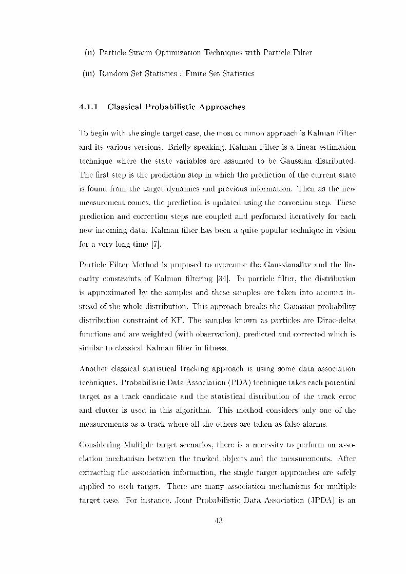
44

Figure 4.2: Explicit/Contour and Implicit/ Grid Representations of Silhouette[42]

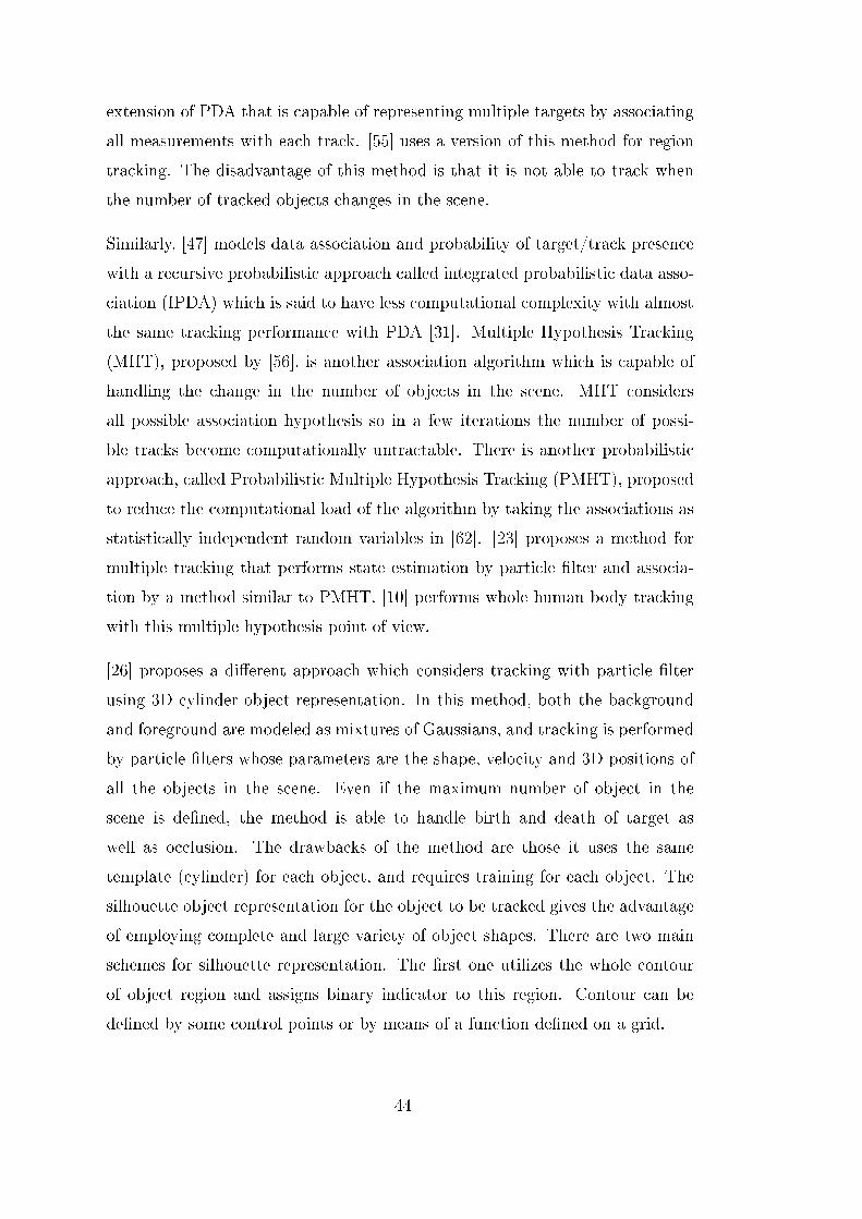
[25] uses contour of the object for tracking. It models the contour shape and

motion as a state vector. This well-known condensation algorithm tracks the

object by means of particle �lter method and the parameters of the particle

�lter are determined by the contour of the object which is a new approach to

tracking scheme. [41] extends this approach to multiple objects by adding an oc-

clusion handling mechanism. Figure 4.4 shows some results of the condensation

algorithm.

45

Figure 4.3: Some Results of Condensation Approach, [25]

[31] brings a new approach for multi-target tracking capabilities of particle �l-

tering methods. When the number of target high, the traditional joint particle

�lter is unusable due to low track quality and high error. An MCMC-based

particle �lter is proposed which brings an improvement on particle �lter that

makes it capable of handling interacting targets. The MCMC-based particle �l-

ter increases the tracking performance compared to standard PF and decreases

the failures reported with the advantage of requiring less number of samples

to track the joint target state. On the other hand this method fails when the

targets in the scene overlap which is a considerably common situation in human

body tracking when the whole human body parts are taken as objects to be

tracked.

There are tracking algorithms speci�cally focused on non-rigid object. The

tracking of a non-rigid object is performed mainly with energy function con-

straint or by using Kalman �ltering under the assumption of Gaussian noise

and knowledge of dynamical model of the object.

In case of deformable non-rigid objects, the object model and target distribution

are nonlinear and non-Gaussian. So, simple Kalman based tracking assumptions

may not be performed. To track non-rigid objects, [50] proposes a vision system

that is able to learn, detect and track the features using mixture particle �lters

and AdaBoost. This article shows the performance of the proposed algorithm

from a hockey match where various number of hockey players in the scene. In

this method, a mixture particle �lter is used for every object being tracked and

46

HSV color space is used to make the tracking more insensitive to illumination

e�ects, since the intensity value is reasonably independent of color. The de-

tection is performed by Bayesian multi-Blob detector and tracker is fed by the

updated detection models. To increase object modeling approximation quality,

the objects are divided into sub-regions according to color and spatial location

and color histograms are created for each sub-regions to form the observation

model.

[57] introduces Kalman and particle �lter usage for lower human body part

tracking considering the human biometrics. The tracking is performed with 2D

model constrained by the human bipedal motion. The experiments performed

in indoor and outdoor sequences give promising tracking results.

4.1.2 Particle Swarm Optimization Techniques with Particle Filter

Particle Swarm Optimization is a population based heuristic optimization tech-

nique which iteratively tries to improve a candidate solution with respect to a

given constraint/objective function [30]. It is a�ected by the organisms behav-

ior/attitude in which each organism make individual motion and able to move

together successfully as a group. The candidate solutions are the particles and

this technique try to update each particle state (position, velocity) by consider-

ing both best local and global positions. In this way, while each particle moves

to their best position, the swarm of particles does not get separated from each

other with the update by the in�uence of global best position. Figure 4.4 shows

a result on global and local best points.

47

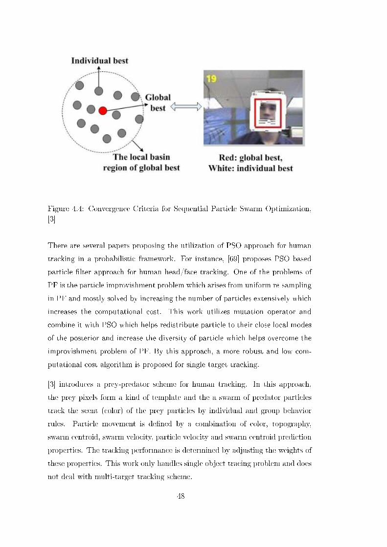
Figure 4.4: Convergence Criteria for Sequential Particle Swarm Optimization,[3]

There are several papers proposing the utilization of PSO approach for human

tracking in a probabilistic framework. For instance, [69] proposes PSO based

particle �lter approach for human head/face tracking. One of the problems of

PF is the particle improvishment problem which arises from uniform re-sampling

in PF and mostly solved by increasing the number of particles extensively which

increases the computational cost. This work utilizes mutation operator and

combine it with PSO which helps redistribute particle to their close local modes

of the posterior and increase the diversity of particle which helps overcome the

improvishment problem of PF. By this approach, a more robust and low com-

putational cost algorithm is proposed for single target tracking.

[3] introduces a prey-predator scheme for human tracking. In this approach,

the prey pixels form a kind of template and the a swarm of predator particles

track the scent (color) of the prey particles by individual and group behavior

rules. Particle movement is de�ned by a combination of color, topography,

swarm centroid, swarm velocity, particle velocity and swarm centroid prediction

properties. The tracking performance is determined by adjusting the weights of

these properties. This work only handles single object tracing problem and does

not deal with multi-target tracking scheme.

48

As [3], [74] uses swarm intelligence perspective for single object human and face

tracking.

49

Figure 4.5: Comparisons between variants of PF and sequential PSO, [3]

Figure 4.5. shows a comparison between PF based methods and PSO approach

for face tracking.

50

Figure 4.6: Experimental Results on Single Object Human Tracking, [74]

Figure 4.6 shows the capability of PSO in human tracking. It is easily seen that

PSO is able to handle clutter, pose and silhouette change and sudden movements

of human body for single object.

Unlike [3] and [74], [15] compares PSO, classical Particle Filter and Enhanced

Particle Filter methods in human tracking and propose that EPF tracker has a

better performance in term of occlusion handling and computational cost.

There are also methods proposed using PSO for multi-target tracking problem

[75, 49].

The advantage of PSO is that it uses the the prior information that the particles

move in coordination unlike utilization of independent particles in the conven-

tional particle �lter method. So PSO is a very meaningful approach in human

tracking since the human body parts move as an inseparable parts of the whole

body.

4.1.3 Finite Set Statistics

Finite set statistics (FISST) is a novel and the �rst systematic approach for

multi-sensor, multi-target tracking [17, 44]. The major problem of FISST was its

combinational complexity. This problem is solved by the Probability Hypothesis

51

Density �lter approximation proposed by Mahler [45].

[71] proposes to use Particle Filter implementation of the PHD �lter for multi-

target tracking. The reason of using particle �lter implementation of PHD is the

use of nonlinear human model. The approach �rst extracts foreground objects

by background subtraction method. It then takes the centroids of the foreground

objects as measurements for PHD �lter. The algorithm results show that this

approach is successful in handling new human entrance, exit and occlusion. The

background in the videos is relatively complex, and birth, merging and disappear

situations are handled successfully. Although the background is complex, it is

�xed in all the frames which make foreground object extraction highly easy and

increase tracking capability.

[43] also utilizes particle based PHD Filters for multi-target tracking. Then

applies K-means method is used for particle clustering, and using the centroid

information of these clusters, association is performed by graph matching to

improve the robustness of the tracking performance.

[70] uses Gaussian Mixture-PHD �lter method for multiple human tracking. The

background is modeled statistically and the background characteristics is con-

structed by the employment of spectral, spatial and temporal features. After

modeling the background, foreground objects are extracted and used as mea-

surement for GM-PHD �lter. The advantage of this method is that it models

birth, survival and death process by number of Gaussian component informa-

tion. This paper uses the same CAVIAR datasets as in [71] for algorithm testing.

This method GM implementation instead of particle �lter approach, so the com-

putational complexity of the algorithm is much [51] employs GM-PHD �lter for

tracking for human tracking from aerial videos. This paper uses aerial videos,

so it deals with homographic correction of the scenes before detection. It uses

RANSAC to handle outliers and performs homography transformation to deal

with camera motion. After handling camera motion, the detection is performed

by intensity-based criteria and GM-PHD �lter is used to track the detected

objects. This method also utilizes Gaussian Mixture Cardinalized PHD �lter

which is a kind of simpli�ed second order moment tracking that propagates car-

52

dinality information. [20] represents the human bodies with moving blobs and

track these by means of PHD �ltering approaches and estimate the unknown

number of persons in the frame. The major advantage of PHD approach is that

it handles association of objects by considering the e�ect of the newly com-

ing measurement to all tracks. This method proposes two di�erent smoothing

technique to PHD �ltering to overcome the miss detection bias and occlusion.

4.2 Deterministic Tracking

Deterministic tracking approaches is mainly grouped into two and detailed in-

formation for these techniques will be provided in this section:

(i) Feature/Template Matching Techniques

(ii) Mean Shift Tracker

4.2.1 Feature/Template Matching Techniques

Template based approaches are those in which the tracking is performed by

measuring the similarities between the template and the current measurement.

In these approaches the templates can be constructed in two di�erent ways. One

of them is to use pre-de�ned templates. Second one is to construct templates

from video and dynamically update them with new information.

The template matching technique is simply a searching mechanism in the image

for a region similar to the object template which is de�ned beforehand. There ex-

ist some similarity measures such as proximity, cross correlation, color/intensity

di�erence. The main aim of template matching is to �nd the location and oc-

currence of the object. The critical point here is in determining the invariant

feature/property of the object.

The representation of the template may alter due to object representation.

In case of patch object representation, the property of the region inside the

53

patch(rectangular, circular) is used and similar region is searched in terms of

the selected property.

There are various versions of patch matching one of which categorize features as

stable, transient and noise [27]. In terms of face tracking of a speaking person,

the stable features are the stationary features as representing nose, transient

ones are the moving features around mouth. The outliers are assumed to be

noise. These features inside the patch are used to de�ne the translation and

warping parameters of the object as well as tracking.

Another method uses Kanade-Lucas-Tomasi (KLT) tracker to �nd the transla-

tion of the region whose center is the interested point. The quality of the tracked

region is determined by a�ne transformation output of the patch between con-

secutive frames.

In multiple object tracking with template matching, [26] proposes a multiple-

layer approach in which di�erent layers are constructed for background and

each object(foreground) in the scene where each object layer comprises shape,

intensity and motion models. Then each pixels probability of belonging to one

of the layers is calculated by means of objects shape and motion characteristic

and the layers are updated with new incoming image properties.

Although these methods are successful from single-view case, they fail as the

object pose/view changes. There are two main approaches dealing with multi-

view case. The �rst one is [4] which performs tracking of articulated objects

by eigen-tracking. In this method object appearance model is constructed using

Principle Component Analysis (PCA) and the image is transformed to the eigen-

space. The a�ne parameters which are the parameters of transformation from

the current object image to the image reconstructed by eigenvectors are found.

Other technique uses, [42], Support Vector Machine Classi�er for tracking. In

case the complete human shape is utilized in tracking, silhouette of the object

is used. There are both deterministic and probabilistic approaches employing

the silhouette of the object for tracking means. Brie�y speaking about the

deterministic approaches, [41, 2, 51] use shape matching schemes whereas [70,

20, 30] employ gradient descent techniques.

54

Tracking using KLT

Kanade-Lucas-Tomasi (KLT) Tracker is an image based tracking algorithm based

on Optical Flow information in the image ([38, 39, 40]). KLT calculates optical

�ow using least squares criterion and assumes that the �ow is constant around

the prede�ned neighborhood of the interested pixel. The calculated �ow is as-

sumed to be hold for all pixels within a window centered at the feature point.

KLT tracker searches the best match of the interested pixel in the next frame.

In general, the pixels are the features extracted by Shi and Tomasi's minimum

eigenvalue method which is optimized feature extraction method for the tracker.

The extracted features are fed to the tracker only in the very �rst frame and KLT

tracks the interested point in the next frames. The features used by KLT are

located by examining the minimum eigenvalue of each 2 by 2 gradient matrix,

and features are tracked by minimizing the di�erence between the two windows.

KLT tracker uses optical �ow information with some basic constraints. The

basic assumptions that;

1. The �ow is constant within a local neighborhood of the feature point of

interest

2. The displacement between consecutive frames is small.

3. The intensity of the patch does not change between two nearby instants.

Comparing (group) tracking methodologies, the working principle of PHD and

KLT is quite di�erent. In KLT the features are extracted in the very �rst

frame and tracked in the next frames by intensity based (in this case optical

�ow) techniques. So when KLT loses the points it is not possible to re-track

of the points. On the other hand, PHD needs measurements in every frame.

So, although the measurements are lost, it is possible to re-track the point if

the feature is extracted in the next frames. In section 6.4, tracking capability of

KLT and the proposed algorithm (GM-PHD) is compared in terms of recognition

performance.The comparison is performed by changing only the tracking block

of the proposed recognition approach. The feature extraction and recognition

55

methods are kept as the same. The fundamental structures of the algorithms

are given in Figure 4.7.

56

Figure 4.7: Structure of applied algorithms for comparison between KLT andGMPHD

The details of the experiments and the results are given in Section 6.4

4.2.2 Mean Shift Tracker

Mean-shift tracking algorithm employs the color/intensity histogram of the ob-

ject being tracked. It compares the histogram of object in the current frame

and histogram of candidate regions in the next frame and �nd the location of

the object in the nexy image iteratively maximizing the correlation between two

histograms. Object tracking for an image frame is performed by a combination

of histogram extraction, weight computation and derivation of new location.

[11] uses circular patch for object representation and uses weighted histogram

property. The method �nds the location of the object by mean-shift tracker

in which the similarity between the color histograms is maximized in terms of

Bhattacharya coe�cient. The advantage of this method is in the searching mech-

anism which decreases the computational complexity. Note that for an accurate

mean-shift tracker the parameters/features should be fed accurately to the ap-

proach. So the initial selection/detection of the patch region has to represent

the object perfectly. Figure 4.8 shows a result of a mean-shift tracker based

approach. As seen it can track the shirt of the child on the image successfully

using color information.

57

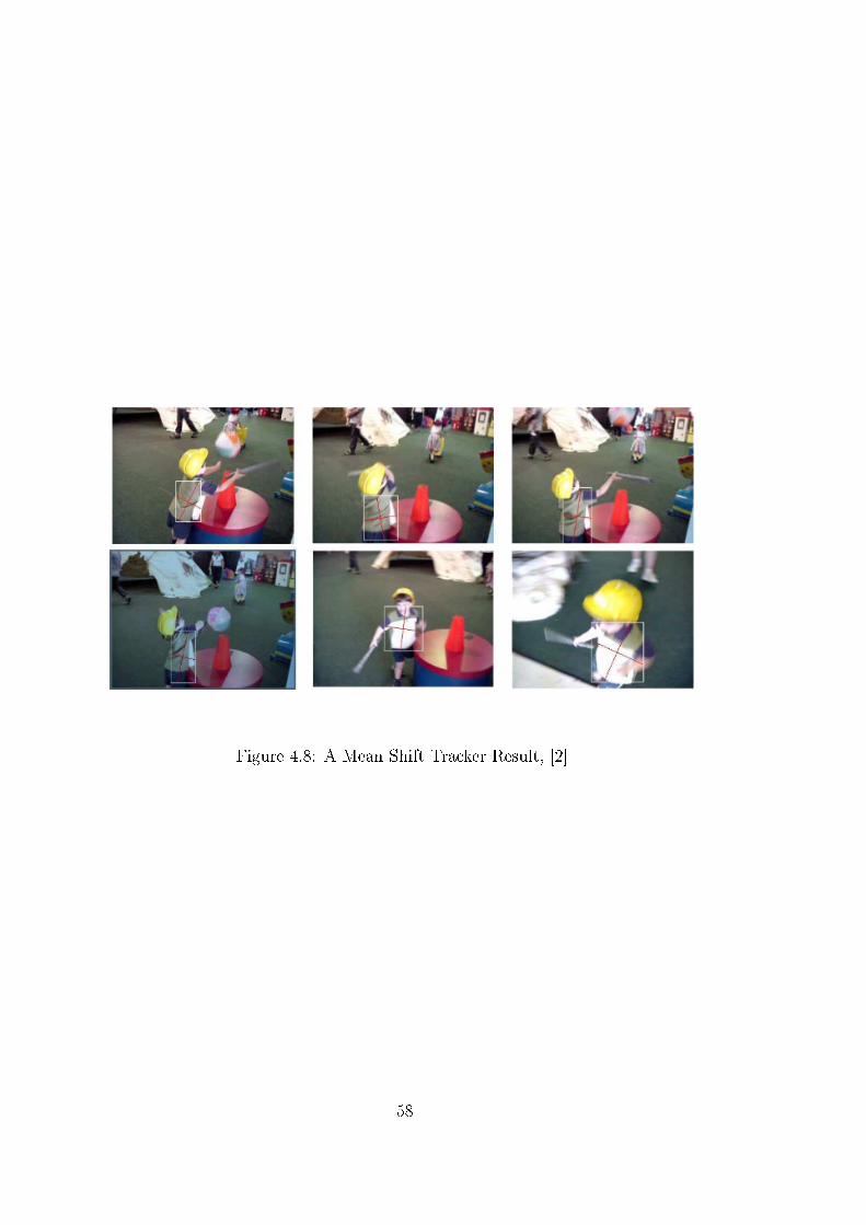
Figure 4.8: A Mean Shift Tracker Result, [2]

58

CHAPTER 5

PROPOSED ACTION RECOGNITION APPROACH

USING GM-PHD AND HMM

Human Action Recognition from visual sources is a quite common approach

which brings some di�culties from its nature. The appearance of the human

in the video is severely a�ected by various factors like complete body motion,

human pose change, independent human body parts' motion and the changes

in the scene itself. The di�culty arises not only from these di�erent motion

a�ects but also the change rate of them. The human body is capable of making

sudden movements of their bodies/pose as well as the individual parts of the

body. In this work we recognize human body by modeling the global and local

body motions.

Considering the video frames as our source, there happens to be information

loss due to projection of 3D nature of human to 2D image view. So, although

the motions of human body are linear, this projection makes the body motion

nonlinear. In addition to this information loss, considering the fact that the

human body is a non-rigid object, the form of the tracked object changes rapidly

as the pose of the body changes. There are various di�erent poses that the human

body may take so the number of possible forms of the silhouette may be too

extensive. As a trivial result, this makes the representation of the human body

more di�cult.

In addition to these, it is likely to face the occlusion problem of the human body.

The occlusion may arise not only from any other object in the scene but also the

local body parts' individual motion. Both of these occlusion types may severely

59

a�ect the appearance of the human body and should be taken into account in

the model.

Human Action Recognition covers the detection, tracking and action recognition

problem. In this thesis we propose a di�erent solution to this problem utilizing

GM-PHD �lter which group tracks the measurements/observations of the human

body as it evolves over time from probabilistic framework. For recognition,

sequential information on human is gathered from visual sources and the best

possible estimate of the hidden variables are investigated using HMM.

In addition to utilize classical state estimates of GM-PHD, GM-PHD distance

and OSPA metric is taken into account for recognition purposes.

The �owchart of the proposed approach is given in 1.1 and 1.2.

In order to crystal clear the feature concept, I want to make some explana-

tions. The image features and the ones used in recognition phase are di�erent.

The image features extracted using Harris Corner Detector are observations and

utilized as measurement for GMPHD Filter. On the other hand, GMPHD �l-

ter estimates and their moments are taken as features for recognition and an

unique HMM is constructed for each feature. The image features are denoted

as observations.

5.1 Observation Extraction by Harris Corner Detector

Selection of observation extraction method is a critical and fundamental step in

action recognition problem. This is because the more robust, discriminative and

informative our observations, the higher performance of action recognition we

obtain.

Observation extraction is the basic step of our action recognition problem. Since

whole frame contains redundant information, we have to eliminate this redun-

dancy and extract the discriminative information on human in action. The

observation extraction method has to be chosen such that it is e�ected from

video problems in minimum order. Considering the general problems, there are

60

occlusion, background change and illumination problems and loss of 3D informa-

tion in video processing approaches. When we focus on our data set, there is a

human body in action and almost constant background which have the following

properties:

1. Articulated object

2. Occlusion of limbs

3. Zooming

4. Illumination change

5. Clutter

6. Shadow

7. Di�erent human characteristics ( carrying a bag, wearing a coat, male,

female, with long hair etc.)

In this thesis, we choose Harris Corner Detector (HCD), [19], as the observation

extractor which generates a point for which there are two di�erent edge directions

in a local neighborhood of the point. The advantage of HCD for articulated

human body is that articulated parts are very likely to have corner points. So,

we have consistent points extracted in consecutive frames. Besides, it is less

a�ected from zooming, illumination change than the other extractor methods.

On the other hand, it unfortunately extracts the observations belonging to the

shadows and di�erent human wearings which have to be eliminated during the

recognition process.

The typical parameters selected for the proposed solution is provided in Table

5.1.

5.2 Group Tracking by GM-PHD

In the tracking phase, all HCD observations are fed to the GM-PHD �lter as

measurements for each frame. Then, GM-PHD �lter produces target intensity

61

Table 5.1: HCD Parameters Selected for the Algorithm.

Parameter Value

Standard deviation of smoothing Gaussian 1Threshold 20

Radius of region considered in non-maximal suppression 1

which is a Gaussian Mixture function. Training and testing phases of action

recognition is performed by extracting information from the Gaussian Mixture

in time.

In this work, target and measurement models together with the related GM-

PHD parameters are provided:

1. State Model: State vector is de�ned as ψ = [x y vx vy]′ and constant

velocity motion model is selected to be as in (5.1).

ψk = Fψk−1 +Gwk−1 (5.1)

where

F =

1 0 ∆t 0

0 1 0 ∆t

0 0 1 0

0 0 0 1

(5.2)

G =

∆t2

20

0 ∆t2

2

∆t 0

0 ∆t

(5.3)

∆t = 1/25 sec. and wk ∼ N (.; 0, 1).

2. Measurement Model: The measurement model is chosen to be as in

(5.4).

62

zk = Hψk + ηk (5.4)

where,

H =

1 0 0 0

0 1 0 0

(5.5)

and ηk ∼ N (.; 0, Rk) with Rk = diag([1, 1]).

3. Clutter (Background Noise) Model: Clutter random �nite set is as-

sumed to be uniformly Poisson distributed as given in (5.6) over the scene

area of 160pixel×120pixel, with λc = 5.2×10−5(pixel)−2. This corresponds

to an average of 1 clutter measurement over the scene of interest.

κk(z) = λcV u(z) (5.6)

where u(.) is the uniform density over the scene, V is the scene area, and

λc is the average number of clutter return per unit area.

4. Detection and Survival Probabilities: Detection and survival proba-

bilities, pD,k and pS,k, are taken as same, which is 0.98.

5. Birth Model: No spawning is assumed and the spontaneous birth inten-

sity is assumed to consist of Gaussian functions uniformly placed over the

scene. Their means are selected to be placed at 10 pixels away from each

other.

γψ(k) =16∑i=1

12∑j=1

wγN (x;mi,jγ , Pγ) (5.7)

where

wγ =0.01/(12× 16) (5.8)

m(i),(j)γ =[5 + (i− 1) ∗ 10, 5 + (j − 1) ∗ 10, 0, 0, 0]′ (5.9)

Pγ =diag(5, 5, 2, 2) (5.10)

where i ∈ 1, 2, . . . , 16 and j ∈ 1, 2, . . . , 12

63

Note that for the rest of the section, GM-PHD �lter output at time k, Dx(x, k),

is assumed to be as in (5.11).

Dψ(ψ, k) =

N(k)∑i=1

wi(k)N (ψ;mi(k), Pi(k)) (5.11)

5.2.1 Utilizing Image Intensity Di�erence in GM-PHD

One of the novelties of this thesis is the use of the intensity di�erence of image

blocks in GM-PHD group tracking phase. The intensity information in the image

is not utilized in standard GM-PHD group tracking approach. There is visual

and powerful information in image which has the capability of increasing the

tracking performance of GM-PHD. So, we use intensity di�erence of the image

blocks centered at GM-PHD states.

Considering GM-PHD as an intensity map, the weights of Gaussian mixtures

are calculated as in Table A.2 of Section A. The �rst two elements of the state

vector corresponds to the positions of the objects. This part of the state vector

is called "position state". We assume that there is small illumination change

around the Position state in-between the consecutive frames.

We use m×n blocks around the position state and compute the intensity di�er-

ence between the image blocks. Then we calculate the mean square di�erence

between the patches as given in (5.12).

∆(k) =1

Nnorps

∥∥Γk|k−1 − Γk−1|k−1

∥∥F

(5.12)

where Γ is 2D image intensity matrix, Nnor is the normalizing factor and ps is the

patch size. F denotes Frobenius norm and the normalizing factor is selected as

51 assuming the maximum intensity di�erence between the pixels in consecutive

frames is 255.

Γk−1|k−1 is chosen as a 5x5 intensity matrix of the gray scale image. The position

of the center element Γ(3, 3) is located at the position estimate belonging to time

64

instant at time k, i.e. xPk−1|k−1 and the center element of Γk|k−1 is chosen at the

predicted state estimate, i.e., xPk|k−1.

The weights in the 'Measurement Update stage' of the GM-PHD �ow is cal-

culated by including the intensity di�erence, ∆(k), into the related equation,

(5.13).

w(lJk|k−1+j)

k = pD,kw(j)k|k−1N (z; η

(i)k|k−1, S

(j)k )(1/∆(k)) (5.13)

∆(k) term is included in the equation (5.13) as division because of intensity

di�erence is inversely proportional to weight. If the intensity di�erence between

the patches is high, this means there is low similarity between the previous and

current location. On the other hand small di�erence implies high similarity

which increases the weight as in (5.13).

5.3 Rotation of Action Direction

In order to use velocity information in action recognition it is essential to convert

all the videos into same type of motion direction. To do this, the velocity com-

ponents of GM-PHD state vectors are transformed into the reference direction.

The rotation process is performed in the way that global motion vector of the

action is extracted and the velocity and covariance components of PHD �lter

are transformed to the reference direction. The rotation process is performed in

the way that global motion vector of the action is extracted and the velocity and

covariance components of PHD �lter are transformed to the reference direction.

The reference direction is chosen to be the right direction and transformation is

performed by �nding the global motion vector and making 2D transformation

of the velocity vectors.

Average velocity of the over-all surface for the jth video is found by taking the

65

velocity components of the average state estimate vector in (5.14).

mjavg =

1

Mj

Mj∑k=1

1

Nj(k)

Nj(k)∑i=1

mji (k) (5.14)

where mji (k) stands for the mean vector for the ith Gaussian in the estimated

PHD and , Nj and Mj corresponds to the number of Gaussians in the PHD at

time k and number of frames for the jth video, respectively. This vector in (5.15)

can also be represented in the polar coordinate system as in (5.16). Direction of

motion is found by simply taking the angle of the mean velocity vector Θjv.

mjv,avg(k) ,[mj

vx,avg(k) mjvy ,avg(k)]′ (5.15)

=

√mjvx,avg(k) +mj

vy ,avg(k)︸︷︷︸Rj

v

, tan−1mjvy ,avg(k)2/mj

vx,avg(k)2︸︷︷︸Θj

v

(5.16)

Then all the velocity components of each videos are transformed in order to

bring all the velocity directions towards the +x direction in average.

mjv(k) =

cos(Θjv) sin(Θj

v)

sin(−Θjv) cos(Θj

v)

mjv(k) (5.17)

where j = 1, . . . , Ntotal and mjv(k) , [mj

vx(k) mjvy(k)]′.

5.4 High Level Recognition by Global Motion Analysis

When we analyze the characteristics of the video, we observe that we can de�ne

a global motion on di�erentiation on running, jogging and walking actions from

the boxing, handclapping and handwaving actions. The analysis of this global

motion makes a high level recognition possible. In High Level Recognition, we

categorize the actions into two groups:

• Group1: Running, Jogging and Walking actions.

66

• Group2: Boxing, Handwaving and Handclapping actions.

In High Level Recognition, x velocity of the motion, mjvx

(k), is utilized for

classi�cation purposes. The actions which has average x velocity greater than

a certain threshold is chosen to be in Group-1 which indicates a global motion

towards x direction. If x velocity is less than a threshold, the action is chosen

to be in Group-2 as given in (5.18).

jth Video ∈

Group− 1, if mjvx ≥ Th px/frame.,

Group− 2, otherwise.(5.18)

where Th indicates the threshold value.

5.4.1 Determination of the Threshold Value

In order to make a classi�cation with x velocity component, mjvx

(k), in an e�-

cient way, �rst we have to eliminate outliers. The outliers are the points belong-

ing to the background and have lower velocity values that decrease the average

velocity and make the discrimination erroneous. It is certain that zooming op-

erations results in a considerable velocity for background observations, yet this

e�ect is ignored for the sake of simplicity. In the �rst step, we eliminate outliers

using position information of the Gaussian Mixture intensity. In elimination,

the GM-PHD modes which are not in an interval determined by standard devi-

ation is discarded. For this purpose, mean and standard deviation of position of

GM-PHD modes are calculated at each frame as given (5.19) and (5.20). Then

the modes which satis�es the conditions given in (5.21) and (5.22) are selected

for High Level Recognition purposes as given in (5.23).

mjx(k) =

1

N j(k)

Nj(k)∑i=1

mji,x(k) (5.19)

67

σjx(k) =

√√√√ 1

N j(k)

Nj(k)∑i=1

(mji,x(k)− mj

x(k))2

(5.20)

cond1(i) =∣∣mj

i,x(k)− mjx(k)

∣∣ < 1.2 ∗ σjx(k) (5.21)

Similarly, mean and standard deviation for the y components are found and

another condition is obtained as in (5.22).

cond2(i) =∣∣mj

i,y(k)− mjy(k)

∣∣ < 2 ∗ σjy(k) (5.22)

ith Mode

∈ Sj(k), if cond1 and cond2 holds,

discard, otherwise.(5.23)

After outlier elimination, HLR threshold value is calculated by using mean of

transformed x velocity information, mji,vx

(k), over L frames as given in (5.24).

mjvx

=1

L

L∑k=1

1

N jS(k)

∑i∈Sj(k)

mji,vx

(k) (5.24)

where NS represents the number of elements in the set Sj(k) and L is selected

as a constant value which is 15.

Then the threshold for HLR operation is chosen by analyzing the mean, mjvx, of

all videos. The histogram of mean of transformed x velocity components over

15 frames,mjvx, of train videos over 15 frames is given in Figure 5.1.

68

Figure 5.1: Histogram of transformed X-Velocity state of GM-PHD

The histogram of, mjvx, reveals us choosing the threshold value as 1.4 makes

HLR possible for GR-1 and GR-2 actions.

5.4.2 Selection of the Group

After determining the threshold value as 1.4 px/frame, the selection of group is

simply performed as in (5.25).

jth Video ∈

Group− 1, if mjvx ≥ 1.4 px/frame.,

Group− 2, otherwise.(5.25)

69

5.5 Determination of Discriminative Modes of GM-PHD

After performing HLR, the way of �nding discriminative modes providing valu-

able information is a critical step for recognition. The discriminative mode

selection is simply choosing the Gaussians of GMPHD which give information

about the foreground object by eliminating the background information. The

outliers are the points that do not belong to the person in action. In the outlier

elimination process, we assume that most of the observations in the frame are

localized on the person taking the action.

The outliers are randomly distributed over the video frame and it may be quiet

di�cult to estimate these points. One of the basic assumptions is that state

estimates belonging to the outliers are far away from the states belonging to the

body and their velocity is much slower than that of the body state estimates.

The selection of discriminative modes are performed in each frame and is per-

formed for both Group-1 and Group-2 action sets in di�erent manners since the

action characteristic is di�erent for each group.

5.5.1 Group-1

In Group-1 action set, we �nd the mean and standard deviation of the x and y

positions of the GM-PHD state estimates as given in (5.27). Then we eliminate

the observations whose positions away from the mean with a constant multiple

of standard deviation given in (5.28) and (5.29).

mjx(k) =

1

N j(k)

Nj(k)∑i=1

mji,x(k) (5.26)

σjx(k) =

√√√√ 1

N j(k)

Nj(k)∑i=1

(mji,x(k)− mj

x(k))2

(5.27)

cond1(i) =∣∣mj

i,x(k)− mjx(k)

∣∣ < 2 ∗ σjx(k) (5.28)

70

Similarly, mean and standard deviation for the y components are found and

another condition is obtained.

cond2(i) =∣∣mj

i,y(k)− mjy(k)

∣∣ < 2 ∗ σjy(k) (5.29)

The outlier elimination process is very similar to HLR but the threshold values.

In outlier elimination using position information, the thresholds are chosen to to

be wider compared to HLR since in HLR a narrower window is more appropriate

in order to take the modes close to body center is su�cient. But in GR-1 we

widen the threshold window in order not to miss the information belonging to

body in action.

In addition to elimination of outliers with respect to position information, the

GM-PHD modes which have lower velocity magnitudes then 0.5 are also elim-

inated. This elimination is performed assuming the fact that there is always a

global displacement of the body in Group-1 videos which result in a consider-

able velocity of the modes in average. Besides since the legs are opened wide,

the standard deviation is not able to eliminate all outliers in the leg part. To

eliminate the GM-PHD modes that have slow motion component, we discard

the features having a speed value less than a constant as given in (5.30). In this

process, one has to be aware the fact that one of the legs stay almost stationary

and we except to lose information regarding that part of the body.

cond3(i) =√mji,vx

(k)2 + mji,vy

(k)2 > 0.5px/frame (5.30)

ith Mode

∈ SjGR-1(k), if cond1, cond2 and cond3 holds,

discarded, otherwise.(5.31)

where SjGR-1(k) represents the selected modes of Gaussian Mixture PHD. Modes

that do not satisfy all the conditions cond1, cond2 and cond3 at the same time

are assumed to be belonging to the background and are eliminated.

71

5.5.2 Group-2

In Group-2 action set, the lower part stands almost the same although the upper

part of the body changes as the hands and arms make clapping, waving and

boxing actions. Since the position information of the lower part is more stable,

we perform elimination of outliers using the information obtained from the lower

part of the body as basis. In the �rst step, we �nd lower part, as explained in 5.6,

of the person and eliminate the outliers using the mean and standard deviation

information calculated as (5.33). position of the this information as given in

(5.35).

Then we eliminate the features whose positions away from the mean with a

constant multiple of standard deviation along only x direction as given in (5.34).

mjx(k) =

1

N j(k)

Nj(k)∑i=1

mji,x(k) (5.32)

σjx(k) =

√√√√ 1

N j(k)

Nj(k)∑i=1

(mji,x(k)− mj

x(k))2

(5.33)

cond1(i) =∣∣mj

i,x(k)− mjx(k)

∣∣ < 1.5 ∗ σjx(k) (5.34)

ith Mode

∈ SjGR-2(k), if cond1 holds,

discarded, otherwise.(5.35)

The outlier elimination approach is very similar to GR1 but the threshold values

and body part. In outlier elimination using position information, the thresholds

are chosen to be narrower compared to GR1 since we make elimination consid-

ering only lower part of the body which do not have motion in general since the

body stands in GR-2 actions.

72

5.6 Clustering

In KTH database actions, the lower and upper part motion characteristics of the

actions are di�erent for both GR-1 and GR-2 actions. So, we choose to analyze

them separately. After eliminating the outliers and determining the discrimina-

tive modes of GMPHD as stated in 5.5, we cluster the GMPHD modes using

position information. The clustering is performed for each group in di�erent

manner. For GR1 actions, the body is clustered into 2 as Upper Part(UP) and

Lower Part(LP) of the body, where as for GR-2 actions, the clustering is made

into 3 as Upper Left(UL), Upper Right(UR) and LP of the body. This cluster-

ing approach is constructed based on body motion of each cluster, since the legs

are wide open in GR1 actions, we prefer to analyze them seperately. In GR-2

actions, although there is slight motion is leg part, discriminative information is

in upper part which has a symmetric motion in hand-clapping and hand-waving

actions which sum up to 3 clusters for GR-2.

Firstly, we mentioen about determination of upper and lower parts, then UL

and UR part extraction is explained.

5.6.1 Determination of Upper and Lower parts for GR-1 and GR-2

After extracting discriminative modes of GMPHD and eliminate outliers, the

determination of Upper and Lower parts is done by simply dividing the body

horizontally into two with 60 percent ratio as given in (5.37). First the height

of the person is calculated using the upper and lower positions along y axis as

given in (5.36).

height = maximji,y(k)−min

imji,y(k), i ∈ SjGR-1(k) (5.36)

We assume that upper and lower parts correspond to head/torso and legs, re-

spectively. To �nd the upper and lower part we perform a simple clustering with

60% ratio. This ratio is selected after analyzing the body motions. We assumed

that leg part of the body consists of 40 percent of the body and performed the

clustering as stated in (5.37).

73

ith Mode

∈ SjGR-1,UP(k), if mj

i,y(k)−minimji,y(k) > 0.6 ∗ height,

∈ SjGR-1,LP(k), otherwise.(5.37)

Similar operations are performed for Group-2 and the body is clustered as Lower

and Upper part.

5.6.2 Determination of Upper-Left and Lower-Left parts for GR-2

For Group-2 actions, it is observed that there exists symmetricity with respect

to the central vertical axis for most of the people in the videos, while this is

not the case for boxing. So we divide the upper part into 2 clusters using the x

center of the lower part of the body which is calculated as given in (5.38). Since

the modes of legs �ts constant velocity model and more robust since there is few

motions, we prefer to take lower part as reference. and for which the dividing

axis is obtained as the x position mean of the lower part as given in (5.38) and

(5.39).

mxL =1

N jGR−2,LP (k)

∑i∈Sj

GR-2,LP(k)

mji,x(k) (5.38)

where N jGR−2,LP (k) corresponds to the number of GM-PHD modes in lower part

of Group-2.

The Upper Left and Upper Right discrimination is performed as stated in (5.39)

ith Mode

∈ SjGR-2,UL(k), if mj

i,x(k) ∈ SjGR-2,UP(k) < meanxL ,

∈ SjGR-2,UR(k), otherwise.(5.39)

5.7 Construction of HMM Structure

In this study, we extract Harris corner observations in each frame and perform

group tracking for these observations by the GM-PHD �lter. GM-PHD make

74

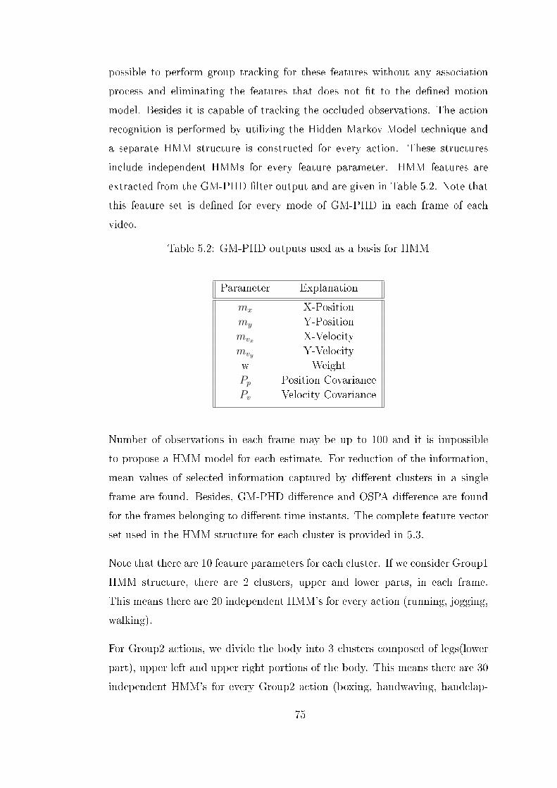
possible to perform group tracking for these features without any association

process and eliminating the features that does not �t to the de�ned motion

model. Besides it is capable of tracking the occluded observations. The action

recognition is performed by utilizing the Hidden Markov Model technique and

a separate HMM structure is constructed for every action. These structures

include independent HMMs for every feature parameter. HMM features are

extracted from the GM-PHD �lter output and are given in Table 5.2. Note that

this feature set is de�ned for every mode of GM-PHD in each frame of each

video.

Table 5.2: GM-PHD outputs used as a basis for HMM

Parameter Explanation

mx X-Positionmy Y-Positionmvx X-Velocitymvy Y-Velocityw WeightPp Position CovariancePv Velocity Covariance

Number of observations in each frame may be up to 100 and it is impossible

to propose a HMM model for each estimate. For reduction of the information,

mean values of selected information captured by di�erent clusters in a single

frame are found. Besides, GM-PHD di�erence and OSPA di�erence are found

for the frames belonging to di�erent time instants. The complete feature vector

set used in the HMM structure for each cluster is provided in 5.3.

Note that there are 10 feature parameters for each cluster. If we consider Group1

HMM structure, there are 2 clusters, upper and lower parts, in each frame.

This means there are 20 independent HMM's for every action (running, jogging,

walking).

For Group2 actions, we divide the body into 3 clusters composed of legs(lower

part), upper left and upper right portions of the body. This means there are 30

independent HMM's for every Group2 action (boxing, handwaving, handclap-

75

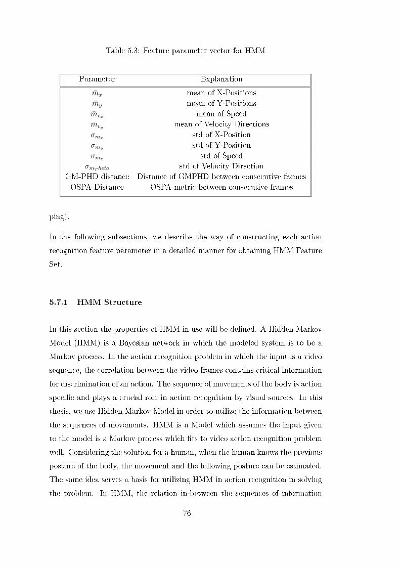
Table 5.3: Feature parameter vector for HMM

Parameter Explanation

mx mean of X-Positionsmy mean of Y-Positionsmvx mean of Speedmvy mean of Velocity Directionsσmx std of X-Positionσmy std of Y-Positionσmr std of Speed

σmT heta std of Velocity DirectionGM-PHD distance Distance of GMPHD between consecutive framesOSPA Distance OSPA metric between consecutive frames

ping).

In the following subsections, we describe the way of constructing each action

recognition feature parameter in a detailed manner for obtaining HMM Feature

Set.

5.7.1 HMM Structure

In this section the properties of HMM in use will be de�ned. A Hidden Markov

Model (HMM) is a Bayesian network in which the modeled system is to be a

Markov process. In the action recognition problem in which the input is a video

sequence, the correlation between the video frames contains critical information

for discrimination of an action. The sequence of movements of the body is action

speci�c and plays a crucial role in action recognition by visual sources. In this

thesis, we use Hidden Markov Model in order to utilize the information between

the sequences of movements. HMM is a Model which assumes the input given

to the model is a Markov process which �ts to video action recognition problem

well. Considering the solution for a human, when the human knows the previous

posture of the body, the movement and the following posture can be estimated.

The same idea serves a basis for utilizing HMM in action recognition in solving

the problem. In HMM, the relation in-between the sequences of information

76

is obtained and hold in by the HMM parameters in the training phase. Then,

in action recognition phase, the most probable HMM is found and the action

owning this HMM is chosen as the recognition result.

As stated before, we use independent HMM structures for each action and each

HMM structure contains one HMM for each feature parameter. After the group

of the action is determined in the High Level Recognition phase, then di�er-

ent HMM structures are constructed for Group1 and Group2 actions which are

provided in Table 5.4 and 5.5.

Table 5.4: Group-1 : Running, Walking and Jogging action properties

Parameter Value

No. of Clusters 2Feature For each Cluster 10General Parameters 2

Total No. of Paramaters 22

Table 5.5: Group-2 : Boxing, Hand-Clapping and Hand-Waving action proper-ties

Parameter Value

No. of Clusters 3Feature For each Cluster 10General Parameters 2

Total No. of Paramaters 32

Notice that in the HMM structure of every action type, there are independent

HMM's for each HMM parameter which sums up to 22 and 32 number of HMM's

for Group-1 and Group-2, respectively.

Talking about the HMM properties, the same HMM frame is used for each

feature of each action which is given in Figure 5.2. The properties of each

HMM frame is given in 5.6. For a detailed information about the properties,

HMM mechanism is explained in 2.3. To mention shortly, Hidden State number

is chosen to be 4 which yields a 1x4 prior probability matrix and a 4x4 state

transition matrix. During the experimentation phase of the thesis, we realize

77

that the hidden number of states, 4, is well su�cient for recognition purposes

for 3 videos. Also note that, we performed some experiments for 3 di�erent

state-transition matrix mechanisms which is mentioned in 6.3.1 in detail.

Considering the representation of outputs, the code-book generation is per-

formed by quantized values of the HMM parameters. So for the code-book

generation i.e., quantization of the HMM parameters is performed and observa-

tion symbols are generated. The calculation of each HMM feature parameter

and data preparation processes are mentioned in Section 5.7.2. Brie�y, in HMM

data preparation phase, every feature is quantized and mapped to 1-11 interval

which directly corresponds to the HMM output states as mentioned in 5.7.2. As

a result, we construct 11 observation symbols whose values can take the integers

between 1 and 11. Since there are 11 observation symbols and 4 hidden models,

the dimension of the observation matrix is of 4x11.

78

Figure 5.2: HMM Frame for each feature of each action

The training phase is performed for the 40% of the videos in the KTH database,

and testing phase is performed with the rest. In the testing phase, after perform-

ing High Level recognition, every sequence belonging to each action is tested by

the trained HMM's of each action. Then the best �tting class of the related fea-

ture is found by taking the class giving out the maximum Posterior Probability.

This recognition process is summarized in Figure 5.3.

79

Figure 5.3: Recognition by HMM

In order to prevent getting stuck to a local maxima and to �nd the global

maxima, we make 20 iterations for the selection of starting point. Best selection

is the point providing the highest likelihood as a result. Then, the resultant

HMM variables are taken for this selection. The convergence criterion for the

HMM is selected to be 0.0001 and maximum iteration number of Baum-Welch

algorithm is selected to be 20.

In recognition phase, every feature sequence of each video is evaluated in 3 in-

dependent HMMs of di�erent actions (Running,Jogging,Walking for Group-1,

Boxing, HandClapping, HandWaving for Group-2). Then the posterior proba-

bilities are calculated and the HMM giving the maximum posterior probability

is selected to be the action belonging to that speci�c feature. This process is

performed for 22 and 32 features for Group-1 and Group-2, respectively. Then

we obtain a 22x1 and 32x1 matrices which guide us for recognition. Finally,

the recognition of action is performed by selecting the action with maximum

occurrence in Feature Decision Vector as given in Tables 6.8 and 6.10.

80

Table 5.6: HMM properties

Parameter Value

Hidden State 4Observation Symbol 11Prior Probability Matrix 1x4State Transition Probability Matrix (3di�erent type)

4x4

Emission Probability Matrix 4x11Iteration Starting point 20Convergence criterion 1e-4Max iteration number 20Training algorithm Baum-WelchTesting (Classi�cation) Criterion Maximum posterior probability,

Max(class)

Feature Decision Vector(FDV) =[ActionDec1,ActionDec2, ...ActionDec22]

(5.40)

No. of Occurrences of FDV =[No. of Act. Type1, No. of Act. Type2, No. of Act. Type3]

(5.41)

Class = max [No. of Act. Type1, No. of Act. Type2, No. of Act. Type3]

(5.42)

5.7.2 Construction of HMM Feature Set

In this section, the way of constructing HMM feature set is explained. As

stated before, Harris corner detector extracts observations for both background

and foreground scene. Based on the assumption that most of the observations

are localized on the human body, we eliminate the features belonging to the

background by some kind of gating using the standard deviation of the overall

information. For a consistent action recognition, it is also necessary to eliminate

81

the e�ects which cause a scaling di�erence in-between di�erent videos and to

map all the HMM features to a prede�ned reference coordinate system. In this

section all the operations which are performed to bring the features to the same

reference is de�ned for every HMM feature. Detailed information on feature

extraction phase for HMM is provided and explanations regarding how we obtain

the feature parameter values used in HMM for action recognition purposes are

given.

5.7.2.1 Mean and Standard Deviation of Position

Human recognizes the action by looking at the person body and limb motion

without considering the background. In parallel to this statement, in action

recognition algorithms, not the position of the feature in the frame but the rela-

tive position of the features with respect to the body center is critical. Another

important observation e�ecting the position of the features is that the height

of the person is di�erent in each frame. This is because of the fact that every

person has di�erent height and the distance between the person and the camera

may be di�erent. We propose a solution for the scaling operation to bring all

types of video sequences to the same reference.

In the �rst step, the uppermost, lowermost, rightmost and leftmost x and y

position limits of are found separately. Then all the positions are mapped to

1-11 interval as given in (5.44).

Y jRange(k) =max

imji,y(k)−min

imji,y(k), i ∈ SjGR-1,UP(k) (5.43)

XjRange(k) =max

imji,x(k)−min

imji,x(k), i ∈ SjGR-1,UP(k) (5.44)

mjq,i,y(k) =(mj

i,y(k)−minimji,y(k))/Y j

Range(k) ∗ 10 + 1, i ∈ SjGR-1,UP(k) (5.45)

mjq,i,x(k) =(mj

i,x(k)−minimji,x(k))/Xj

Range(k) ∗ 10 + 1, i ∈ SjGR-1,UP(k) (5.46)

82

The equation is given for the Upper part of GR-1 actions. Same operations are

performed for all 3 clusters of GR-2 and lower part of GR-1.

After mapping the values to the interval [1-11], mean and std of the x-position

and y-positions are found for each cluster. Finally, quantization is performed by

the rounding operation and the HMM feature parameter values related to the

positions are obtained as in (5.48).

meanjmq,x(k) =round

1

N jGR−1,UP (k)

∑i∈Sj

GR-1,UP(k)

mjq,i,x(k) (5.47)

meanjmq,y(k) =round

1

N jGR−1,UP (k)

∑i∈Sj

GR-1,UP(k)

mjq,i,y(k) (5.48)

σjmq,x(k) =round

√√√√ 1

N j(k)

Nj(k)∑i=1

(mjq,i,x(k)− mj

q,x(k))2

(5.49)

σjmq,y(k) =round

√√√√ 1

N j(k)

Nj(k)∑i=1

(mjq,i,y(k)− mj

q,y(k))2

(5.50)

5.7.2.2 Mean and Standard Deviation of Speed

The distance between the person and the camera varies both within the video

frames and within di�erent types of videos. As a result, the height of the person

observed for both within a video sequence and for di�erent videos varies. In

order to overcome this problem, calculated height of the person in action is

mapped to a reference height. The diversity of the distance of the person to the

camera also a�ects the velocity components. In order to work in the same scale

the velocity is also transformed to a reference.

Proposed GMPHD state de�nition includes velocities along x and y directions.

By taking the velocity components of the state estimates into account, speed

information is obtained as in equation (5.16).

Since speed is extracted using 2D image domain, speed of the person changes as

83

the position of the person to the camera changes. So, if we want to use speed

information in action recognition, it is necessary to use the same speed scale in

all videos.

In order to obtain the reference, we perform a post processing operation and

obtain the height range of the person from all videos given in Figure 5.4 and the

range is selected as RefHeight = 110.

84

Figure 5.4: Histogram of Height of person in action in KTH database.

The feature set related to speed information is obtained by:

i Person height in the frame is found by taking di�erence upper and lower

Y position as given in (5.36).

ii Speed is transformed to a domain independent from person height and

position with respect to the camera.

Rjvi,m

(k) =Rjvi

(k) ∗RefHeight/Height (5.51)

iii Speed value is delimited to 0-15 (SpeedLimit = 15) interval after analyzing

the speed by obtaining speed histogram given in Figure 5.5.

85

Figure 5.5: Histogram of Speed of person in action in KTH database.

Then the delimited speed is mapped to 1-11 interval as given in (5.52)

Rjvi,q

(k) = Rjvi,m

(k)/SpeedLimit ∗ 10 + 1 (5.52)

iv Mean and std. of speed vectors is found for each cluster as given in (5.53)

and (5.54)

Rjvi,q

(k) = round1

N jGR−1,UP (k)

∑i∈Sj

GR-1,UP(k)

Rjvi,q

(k) (5.53)

σRjvi,q

(k) =round

√√√√ 1

N j(k)

Nj(k)∑i=1

(Rjvi,q(k)− Rj

vi,q(k))2

(5.54)

Mean and standard deviation of speed information belonging to GR-1

lower part and all parts of GR-2 is calculated in the same manner.

86

5.7.2.3 Mean and Standard Deviation of Angle

When we consider the direction of body motion, the �rst prominence is that

it changes between videos. In other words, the body moves along di�erent

directions. In order to use velocity angle for action discrimination purposes, we

need to map the angle to a reference direction.

i Velocity Angle is transformed towards the right direction

In order to construct a reference, global motion vector of the motion is

extracted and the velocity is transformed to the reference direction as

explained in 5.3.

In analyzing Velocity Angle, we investigated the correlation of speed with

angle. We performed this analysis since in HMM recognition they are

taken as independent. If there are any correlation we might have miss the

information. So, the velocity speed vs. angle map is constructed for GR-1

actions to visualize the relationship which is given in Figure 5.6.

For a more detailed analysis, histogram is obtained by dividing the body

into 3 portions which correspond to head,torso and foot respectively. The

�gure indicates that there is no direct correlation between the components

which make us decide to use speed and angle information independently.

87

Figure 5.6: Histogram Speed vs Velocity Angle of GR-1 actions

ii Velocity angle limits are taken as to cover 2 *pi range after analyzing the

velocity direction by obtaining angle histogram given in Figure 5.7.The

analysis performed for GR-1 actions since it is obvious that hand-waving

operation covers 2π range. So following values for the related parameters

are taken in the algorithms:

AngleLimit =π (5.55)

Minangle =π (5.56)

88

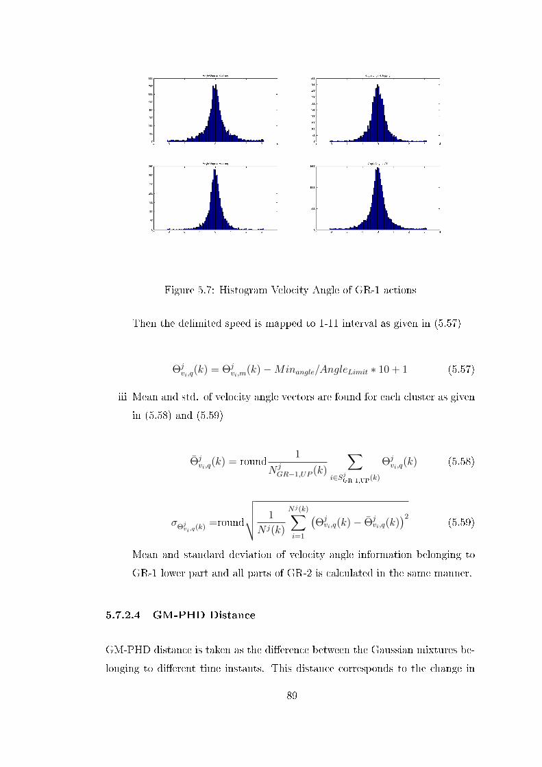
Figure 5.7: Histogram Velocity Angle of GR-1 actions

Then the delimited speed is mapped to 1-11 interval as given in (5.57)

Θjvi,q

(k) = Θjvi,m

(k)−Minangle/AngleLimit ∗ 10 + 1 (5.57)

iii Mean and std. of velocity angle vectors are found for each cluster as given

in (5.58) and (5.59)

Θjvi,q

(k) = round1

N jGR−1,UP (k)

∑i∈Sj

GR-1,UP(k)

Θjvi,q

(k) (5.58)

σΘjvi,q

(k) =round

√√√√ 1

N j(k)

Nj(k)∑i=1

(Θjvi,q(k)− Θj

vi,q(k))2

(5.59)

Mean and standard deviation of velocity angle information belonging to

GR-1 lower part and all parts of GR-2 is calculated in the same manner.

5.7.2.4 GM-PHD Distance

GM-PHD distance is taken as the di�erence between the Gaussian mixtures be-

longing to di�erent time instants. This distance corresponds to the change in

89

the Gaussian mixture functions, including all positional, velocity, weight and co-

variance information in time. In this thesis, the distance is taken for consecutive

frames. De�nition and calculation of this distance is provided in this section.

Remembering the GM-PHD is a Gaussian Mixture function as given in (5.60),

the function to �nd the distance between PHD's belonging to di�erent time

instants,i.e, k1 and k2, is proposed as in (5.61).

p(x, k) =

N(k)∑i=1

wi(k)N (x;mi(k), Pi(k)) (5.60)

D(k1, k2) =

∫(p(x, k1)− p(x, k2))2dx (5.61)

If the subtraction in (5.61) is focused, another Gaussian mixture function is

obtained.

p(x, k1)− p(x, k2) =

N(k1)+N(k2)∑n=1

wn(k1, k2)N (x;mn(k1, k2), Pn(k1, k2)) (5.62)

where

wn(k1, k2) ={w1(k1), . . . , wN(k1)(k1),−w1(k2), . . . ,−wN(k2)(k2)}N(k1)+N(k2)n=1

(5.63)

mn(k1, k2) ={m1(k1), . . . ,mN(k1)(k1),m1(k2), . . . ,mN(k2)(k2)}N(k1)+N(k2)n=1 (5.64)

Pn(k1, k2) ={P1(k1), . . . , PN(k1)(k1), P1(k2), . . . , PN(k2)(k2)}N(k1)+N(k2)n=1 (5.65)

(5.66)

Taking the square of the Gaussian Mixture function in (5.61), (5.67) is found.

(p(x, k1)− p(x, k2))2 =

N(k1)+N(k2)∑n=1

N(k1)+N(k2)∑p=1

wnwpN (x;mn, Pn)N (x;mp, Pp)

(5.67)

(5.67) includes multiplication of two Gaussian functions which results in another

Gaussian multiplied by a scalar, (5.68).

90

N (x;mn, Pn)N (x;mp, Pp) = N (mn;mp, Pp + Pn)N (x;mn|p, Pn|p) (5.68)

where

mn|p = (P−1n + P−1

p )−1(P−1n mn + P−1

p mp) (5.69)

Pn|p = (P−1n + P−1

p )−1 (5.70)

Inserting (5.68) to (5.67) and then inserting (5.67) to (5.61), the distance be-

tween two Gaussian Mixtures belonging to di�erent time instants are found as

in (5.71)

D(k1, k2) =

N(k1)+N(k2)∑n=1

N(k1)+N(k2)∑p=1

wnwpN (mn;mp, Pp + Pn) (5.71)

5.7.2.5 Optimal SubPattern Assignment (OSPA) Metric

OSPA distance is proposed by [59] and serves as a metric providing information

regarding the di�erence between two �nite sets. Input for the OSPA function

are generally taken as the state estimates set of the PHD �lter and true target

state set. This metric takes both the di�erence between the state positions and

the di�erence in the set cardinalities into account.

Properties of OSPA provided in [59] are brie�y listed in as below:

• a metric on the space of �nite sets,

• a natural (meaningful) physical interpretation,

• taking the cardinality errors and state errors into account meaningfully,

• easy computation.

OSPA metric is widely used for performance evaluation of the multi-target

state estimators. In the case of this thesis, there does not exist the ground

91

true target set yet this distance is utilized for �nding the di�erence between

given two state estimate set belonging to di�erent time instants of the video,

X(k1) = {x1(k1), . . . , xm(k1)} and X(k2) = {x1(k2), . . . , xn(k2)}, where X is the

estimated feature position set and m,n ∈ N0 = {0, 1, 2, . . .}. The equation of

the metric of order p with cut-o� c is proposed by [59] as in (5.72).

d(c)

p (X(k1), X(k2)) :=

(1

n

(minπ∈Πn

m∑i=1

d(c)(xi(k1), xΠ(i)(k2))p + cp(n−m)

))(5.72)

For any vector x and y, the parameters in (5.72) are described as:

• dc(x, y) := min(c, d(x, y))

• c > 0: cut-o�

• Πk: the set of permutations on {1, 2, . . . , k} for any k ∈ N = {1, 2, . . .}

• d(x, y): L2 norm distance between the vectors

The distance (5.72) is calculated for m ≤ n and 1 ≤ p < ∞. In case m > n,

d(c)

p (X(k1), X(k2)) is found as d(c)

p (X(k2), X(k1)).

Note that in this thesis, the OSPA metric of order 2 with cut-o� 10 is chosen for

�nding the di�erence between the frames belonging to di�erent time instants.

The state estimates are taken as the positional information of the mean values

belonging to di�erent modes of the Gaussian Mixture PHD, whose weights are

greater than 0.5.

92

CHAPTER 6

PERFORMANCE EVALUATION OF THE PROPOSED

APPROACH

In this chapter, we give performance results of the proposed approach for the

videos taken in a controlled environment including KTH Database and custom

taken occlusion videos. Firstly, we give detailed information about the controlled

databases, KTH and custom taken occlusion videos. Then, we give detail infor-

mation about the experiments which are performed with di�erent parameters.

After explaining the experiments, the performance results of each experiment

is given as both correctly recognized video percentages and related confusion

matrices in KTH database.

Besides, we analyze the e�ect of using KLT as an alternative to GMPHD on the

tracking phase and provide corresponding recognition performance.

Finally, we compare the proposed approach with a well known algorithm, [54],

which is denoted as base algorithm, for custom occlusion scenarios and reveal

the recognition performances on custom 6 videos taken for this thesis.

6.1 KTH Database

In this thesis, we used KTH video database as a controlled database for action

recognition problem. There are 25 individuals performing 6 type of actions:

• Jogging

93

• Running

• Walking

• Handwaving

• Handclapping

• Boxing

in 4 di�erent environments:

• d1: outdoors

• d2: outdoors with scale variation

• d3: outdoors with di�erent clothes

• d4: indoors

with a frame size 160× 120 and 25 frame/second as given in original paper [60].

Figure 6.1 shows a frame example of each type.

94

Figure 6.1: Example frames of each video in KTH Database

In this work, we grouped these according to global motion occurrence in the

action as given in Table 6.1.

Table 6.1: De�ned Groups in the Context of the Thesis

Group Name Action

Group-1 Jogging, Running, WalkingGroup-2 Boxing, Hand Clapping, Hand Waving

Group1 (GR1) actions are the ones with global motion. In these videos, the

body in action moves toward one direction. The motion direction of the human

body varies as stated below:

1. Motion towards the right direction

2. Motion towards the left direction

3. Diagonal motions towards the lower right and left corners

4. Diagonal motions towards the upper right and left corners

Group-2 actions are the ones without global motion. The person performing the

boxing, handclapping, handwaving actions in the video is stationary and the

action is caused by the movement of the arms. Videos on the database have

speci�c di�erent characteristics containing:

95

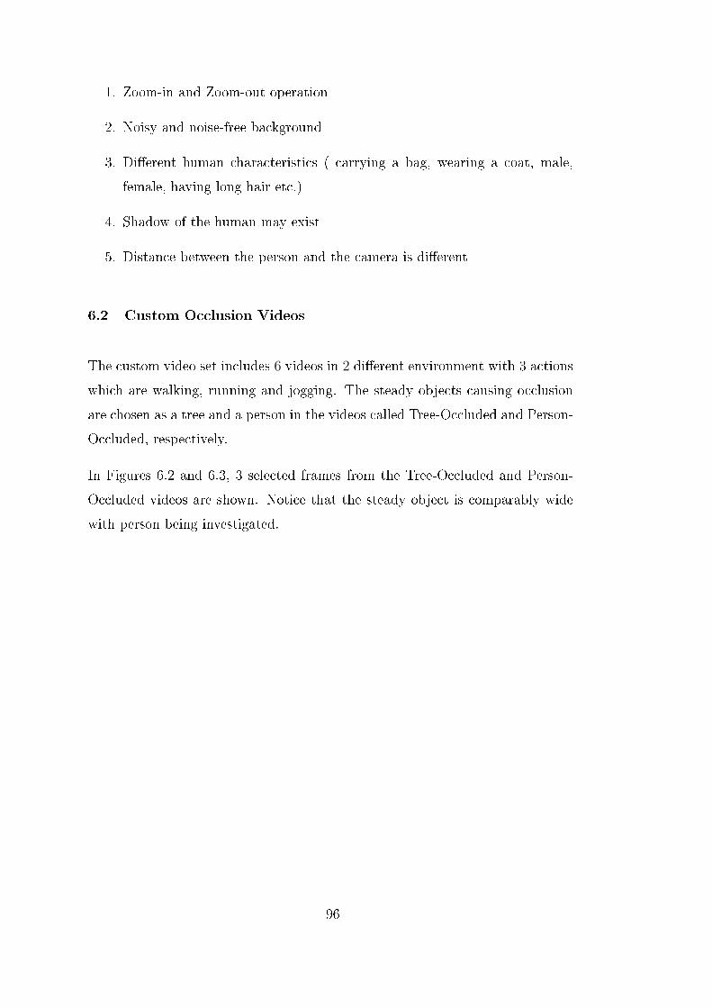
1. Zoom-in and Zoom-out operation

2. Noisy and noise-free background

3. Di�erent human characteristics ( carrying a bag, wearing a coat, male,

female, having long hair etc.)

4. Shadow of the human may exist

5. Distance between the person and the camera is di�erent

6.2 Custom Occlusion Videos

The custom video set includes 6 videos in 2 di�erent environment with 3 actions

which are walking, running and jogging. The steady objects causing occlusion

are chosen as a tree and a person in the videos called Tree-Occluded and Person-

Occluded, respectively.

In Figures 6.2 and 6.3, 3 selected frames from the Tree-Occluded and Person-

Occluded videos are shown. Notice that the steady object is comparably wide

with person being investigated.

96

Figure 6.2: Frames from the Tree Occlusion Test Videos

Figure 6.3: Frames from the Person Occlusion Test Videos

97

Talking about the videos they are taken without using tree-pot, so there is slight

motion in the videos. As the environment, they are taken outside and Tree-

Occlusion video has more outlier measurements/features which makes recogni-

tion di�cult.

6.3 Experimental Results on KTH Database

The experiments of the proposed algorithm is performed using the well-known

KTH database. And the performance evaluation is done using approximately

50% percent of the videos in KTH database.

6.3.1 Experimental Parameters

Frame Size:

We determine the frame size of the video according the group type. For GR1

actions, the running action determines the frame size since it takes less frame

to pass the person in the scene.

Table 6.2: Frame Number for the Groups

Group No Frame Size

Group-1 14Group-2 20

Windowing Method:

We implemented 3 di�erent windowing methods as given in Table 6.3.

Table 6.3: Selections of Windowing Type

Windowing Method Window Size

No windowing XStandart Windowing 3

Sliding window 5

98

In �No windowing� case, we do not perform any windowing operation. Instead,

feature vector of each frame is taken and HMM recognition is performed within

the information in each frame itself. The place of the operation in the �ow-chart

is given in 6.4.

99

Figure 6.4: Windowing Operations in Flow Chart

In the 2nd windowing approach, we take window size as 3. The feature vector is

obtained bu calculating the mean of features for 3 frames. Note that we perform

a mean operation in each cluster of each frame. The windowing operation in the

FlowChart is given in Figure 6.4.

100

Figure 6.5: Structure of Windowing Method-2

Sliding window approach is utilized as the 3rd windowing operation,6.4. The

approach is given in Figure 6.6.

101

Figure 6.6: Structure of Windowing Method-3

In sling window technique, we obtain feature vector by taking the mean of

windows with size 5. In this method, mean operation is performed using the

current and previous 4 frame's feature vectors.

HMM Types:

The experiments are performed with using 3 di�erent HMM types to understand

the a�ect of HMM type to recognition performance. HMM Types are given in

Table 6.4.

Table 6.4: Selections of HMM Type

HMM Type Explanation

Type-0 Full HMMType-1 Forward HMMType-2 Half HMM

Type-0 HMM is ergodic, fully connected one in which we expect transitions

102

Figure 6.7: Type-0: Fully Connected HMM State Flow

between all hidden states as given in Figure 6.7.

Type-1 HMM is forward connected one in which we expect transitions along for-

ward direction given in Figure 6.8. In action recognition case, when we consider

one cycle of action, Type-1 HMM is appropriate.

103

Figure 6.8: Type-1: Forward Connected HMM State Flow

Type-2 HMM is called half connected HMM in which there is one backward

connection to the �rst hidden state is added compared to Type-1 HMM. This

structure is formed considering the existence of cyclic operations in action. The

connections are given in Figure 6.9.

104

Figure 6.9: Type-2: Half Connected HMM State Flow

6.3.2 Selection of Training Elements

An unique HMM is constructed for each of the feature which is given in Section

5.7 in detail. When we extract these properties of each cluster we obtain 22 and

32 independent HMMs for GR1 and GR2 respectively. The features are listed

in the Tables 6.56.6 for GR1 and GR2 action groups respectively.

As mentioned in 5, GR1 has 2 clusters and GR2 has 3 clusters each of which

has 10 features. Adding 2 features belonging to body we obtain 22 HMMs for

GR1 and 32 HMMs for GR2.

In the experiments, 22 and 32 number of observation sequences are extracted

from the video as given in 6.10. Note that Z corresponds to 22 and 32 for GR1

and GR2, respectively.

105

Table 6.5: Group-1 Training Elements

Element No Feature Property Body Segment

1 X Position Upper Part of the Body2 X Position Lower Part of the Body3 Y Position Upper Part of the Body4 Y Position Lower Part of the Body5 Direction of Motion Upper Part of the Body6 Direction of Motion Lower Part of the Body7 Speed Upper Part of the Body8 Speed Lower Part of the Body9 X Position Std. Dev. Upper Part of the Body10 X Position Std. Dev. Lower Part of the Body11 Y Position Std. Dev. Upper Part of the Body12 Y Position Std. Dev. Lower Part of the Body13 Direction of Motion Std. Dev. Upper Part of the Body14 Direction of Motion Std. Dev. Lower Part of the Body15 Speed Std. Dev. Upper Part of the Body16 Speed Std. Dev. Lower Part of the Body17 GM Di�erence Upper Part of the Body18 GM Di�erence Lower Part of the Body19 OSPA Upper Part of the Body20 OSPA Lower Part of the Body21 GM Di�erence Whole Body22 OSPA Whole Body

106

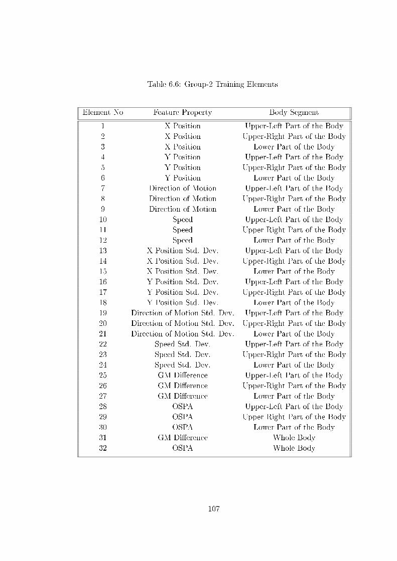
Table 6.6: Group-2 Training Elements

Element No Feature Property Body Segment

1 X Position Upper-Left Part of the Body2 X Position Upper-Right Part of the Body3 X Position Lower Part of the Body4 Y Position Upper-Left Part of the Body5 Y Position Upper-Right Part of the Body6 Y Position Lower Part of the Body7 Direction of Motion Upper-Left Part of the Body8 Direction of Motion Upper-Right Part of the Body9 Direction of Motion Lower Part of the Body10 Speed Upper-Left Part of the Body11 Speed Upper-Right Part of the Body12 Speed Lower Part of the Body13 X Position Std. Dev. Upper-Left Part of the Body14 X Position Std. Dev. Upper-Right Part of the Body15 X Position Std. Dev. Lower Part of the Body16 Y Position Std. Dev. Upper-Left Part of the Body17 Y Position Std. Dev. Upper-Right Part of the Body18 Y Position Std. Dev. Lower Part of the Body19 Direction of Motion Std. Dev. Upper-Left Part of the Body20 Direction of Motion Std. Dev. Upper-Right Part of the Body21 Direction of Motion Std. Dev. Lower Part of the Body22 Speed Std. Dev. Upper-Left Part of the Body23 Speed Std. Dev. Upper-Right Part of the Body24 Speed Std. Dev. Lower Part of the Body25 GM Di�erence Upper-Left Part of the Body26 GM Di�erence Upper-Right Part of the Body27 GM Di�erence Lower Part of the Body28 OSPA Upper-Left Part of the Body29 OSPA Upper-Right Part of the Body30 OSPA Lower Part of the Body31 GM Di�erence Whole Body32 OSPA Whole Body

107

Figure 6.10: An Individual HMM structure

108

In training phase, all HMM parameters in the HMM structure are trained with-

out making any intelligent selection among the HMMs. In testing phase, again

all the recognition results for each video for each HMM is obtained. Then as a

post processing optimal selection of features is performed which gives the

6.3.3 Experimented Approaches and Their Performances

The recognition performance of all 9 methods are given in this section. Table 6.7

and Table 6.9gives the performance of the proposed algorithm for each method

for GR1and GR2 actions, respectively. The designated results are obtained by

optimal selection of features as given in Tables 6.8 and 6.10. After evaluating

the output of each HMM and optimal selection is made utilizing these results.

Table 6.7: Methods and Performances for Group-1

MethodNo

WindowingType

HMMType

Perf. forAll Videos

1 1 0 89.38%2 1 1 86.88%3 1 2 86.88%4 3 0 85%5 3 1 86.25%6 3 2 83.75%7 5 0 82.5%8 5 1 83.13%9 5 2 82.5%

The numbers in Tables 6.8 and Table 6.10 refer to the feature numbers given

in Tables 6.5 and 6.6, respectively. The order has the meaning that the ratio

of correct recognition increases to the right direction. To speak specially, 19 is

number of feature with highest score of the �rst row of Table 6.8.

Analyzing the results, it is seen that Method1 has the highest recognition per-

formance which is of ergodic HMM type and has no windowing operation.

Similar experiments are performed for Group2(GR2) actions and the results

reveals that Method2 has the highest recognition performance for GR2 actions

109

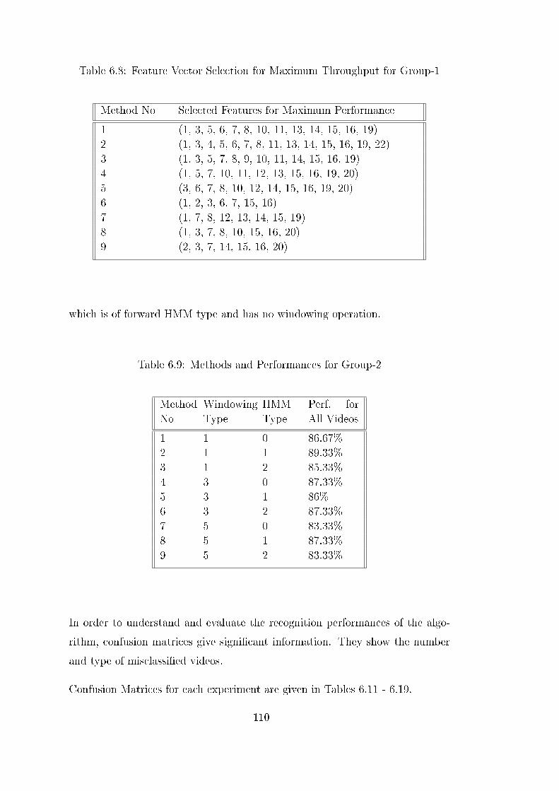
Table 6.8: Feature Vector Selection for Maximum Throughput for Group-1

Method No Selected Features for Maximum Performance

1 (1, 3, 5, 6, 7, 8, 10, 11, 13, 14, 15, 16, 19)2 (1, 3, 4, 5, 6, 7, 8, 11, 13, 14, 15, 16, 19, 22)3 (1, 3, 5, 7, 8, 9, 10, 11, 14, 15, 16, 19)4 (1, 5, 7, 10, 11, 12, 13, 15, 16, 19, 20)5 (3, 6, 7, 8, 10, 12, 14, 15, 16, 19, 20)6 (1, 2, 3, 6, 7, 15, 16)7 (1, 7, 8, 12, 13, 14, 15, 19)8 (1, 3, 7, 8, 10, 15, 16, 20)9 (2, 3, 7, 14, 15, 16, 20)

which is of forward HMM type and has no windowing operation.

Table 6.9: Methods and Performances for Group-2

MethodNo

WindowingType

HMMType

Perf. forAll Videos

1 1 0 86.67%2 1 1 89.33%3 1 2 85.33%4 3 0 87.33%5 3 1 86%6 3 2 87.33%7 5 0 83.33%8 5 1 87.33%9 5 2 83.33%

In order to understand and evaluate the recognition performances of the algo-

rithm, confusion matrices give signi�cant information. They show the number

and type of misclassi�ed videos.

Confusion Matrices for each experiment are given in Tables 6.11 - 6.19.

110

Table 6.10: Feature Vector Selection for Maximum Throughput for Group-2

Method No Selected Features for Maximum Performance

1 (2, 3, 4, 8, 14, 16, 22, 23, 29, 32)2 (2, 3, 4, 5, 8, 11, 14, 15, 20, 22, 23, 32)3 (1, 2, 5, 8, 10, 14, 15, 17, 22, 23, 29, 32)4 (1, 2, 3, 10, 11, 14, 15, 22, 23, 28, 30, 32)5 (1, 2, 5, 7, 10, 11, 14, 23, 32)6 (1, 3, 4, 5, 10, 14, 15, 23, 30, 31, 32)7 (1, 2, 3, 5, 8, 10, 11, 13, 16, 22, 23, 26, 28)8 (2, 5, 7, 10, 11, 14, 15, 22, 23, 28)9 (1, 2, 5, 10, 13, 14, 16, 17, 22, 23, 26, 28, 32)

Table 6.11: Confusion Matrix for Windowing Type:1 and HMM Type:0

- Jg. Rn. Wl. Bx. Hc. Hw.

Jg. 45 5 0 0 0 0Rn. 5 44 0 0 0 0Wl. 5 2 54 0 0 0Bx. 0 0 0 42 3 2Hc. 0 0 0 2 42 6Hw. 0 0 0 1 6 46



Jg. 42 6 1 0 0 0Rn. 4 43 2 0 0 0Wl. 9 2 51 0 0 0Bx. 0 0 0 39 3 0Hc. 0 0 0 4 41 3Hw. 0 0 0 2 7 51

6.3.4 The E�ect of OSPA Parameter on the Performance

In this section, the e�ect of OSPA parameter on the recognition performance

is investigated. The 'Feature Set without OSPA' result given in Table 6.20 is

obtained by excluding the HMM structures trained by OSPA parameters. For

111



Jg. 42 6 1 0 0 0Rn. 4 43 2 0 0 0Wl. 9 2 51 0 0 0Bx. 0 0 0 39 3 0Hc. 0 0 0 4 41 3Hw. 0 0 0 2 7 51



Jg. 41 5 0 0 0 0Rn. 7 44 0 0 0 0Wl. 7 2 54 0 0 0Bx. 0 0 0 40 5 2Hc. 0 0 0 2 44 2Hw. 0 0 0 3 2 50



Jg. 42 7 0 0 0 0Rn. 4 42 0 0 0 0Wl. 9 2 54 0 0 0Bx. 0 0 0 38 4 2Hc. 0 0 0 4 42 3Hw. 0 0 0 3 5 49

Group 1 actions we exclude OSPA for upper,lower and whole body parts, for

Group 2 actions we exclude OSPA for upper-left, upper-right,lower and whole

body parts.

DiscussionWhen we analyze the results, we see that OSPA parameter makes a

3% improvement on recognition performance for Group2 actions. On the other

hand it makes no improvement for Group1 actions. From these results we can

conclude that the OSPA parameter is not a fundamental but auxiliary parameter

112



Jg. 41 6 3 0 0 0Rn. 7 41 0 0 0 0Wl. 7 4 51 0 0 0Bx. 0 0 0 41 5 2Hc. 0 0 0 2 41 3Hw. 0 0 0 2 5 49



Jg. 41 6 0 0 0 0Rn. 6 44 0 0 0 0Wl. 8 1 54 0 0 0Bx. 0 0 0 40 7 2Hc. 0 0 0 4 41 5Hw. 0 0 0 1 3 47



Jg. 34 3 2 0 0 0Rn. 11 48 0 0 0 0Wl. 10 0 52 0 0 0Bx. 0 0 0 42 3 2Hc. 0 0 0 2 44 7Hw. 0 0 0 1 4 45

for action recognition.

6.3.5 Discussions

In this chapter, we give the performance results of the proposed algorithm in

9 di�erent experiments with 3 di�erent HMM model and 3 di�erent windowing

techniques.

113



Jg. 39 6 2 0 0 0Rn. 8 42 1 0 0 0Wl. 8 3 51 0 0 0Bx. 0 0 0 37 4 3Hc. 0 0 0 3 45 8Hw. 0 0 0 5 2 43

Table 6.20: GMPHD Results for the Feature Sets Including and not IncludingOSPA Distance

GR1 GR2

Feature Set with OSPA 89.38% 89.33%Feature Set without OSPA 89.38% 86.00%

When we analyze the results, the highest performance is achieved for the ergodic

HMM for GR1. This is meaningful since the observation data may not contain

one cycle of information. So the connection between all states have been neces-

sary. On the other hand, GR2 has the greatest performance with HMM type-1

since the size of the data is long enough to complete one cycle of the action.

Comparing the window size results, the best is achieved in no windowing case for

both GR1 and GR2 videos. The reason for this is the reduction in the number

of sequence in the observation space for window size 3.Since the observation

sequences are not long enough, windowing processes lead loss of data, and the

results obtained with the complete data give the best results. For sliding-window

technique, i.e. window size is 5, the low-pass �ltering (mean operation) results

in the reduction of informative data between the frames and when we analyze

data in a video, we see that sliding window approach brings the information in

the frame to almost same level.

Talking about the selection of features, speed brings out the most informative

feature among all for all videos. Speed as well as its standard deviation carries

critical information belonging to the action. In addition to the speed, X position,

114

Y position, direction of upper part and body OSPA di�erences (for GR2) are

discriminative features as given in �rst row of 6.8 and 2nd row of 6.10.

Note that OSPA metric obtained by considering the whole body positions plays

a critical role in action recognition of GR2 actions.

We see that GM-PHD distance parameter is not a consistent parameters when

we consider the distance between the consecutive frames. It is observed that

this inconsistency is caused by the sensitivity of the distance to the covariance

information, which can take broad range of values for di�erent features and

di�erent time frames.

Another important observation regarding GMPHD �lter is that Harris corner

detector is not capable of extracting consistent observation points in the videos

in consideration due to illumination changes. In some frames Harris may not

�nd some critical points. In these cases PHD is able to compensate the low

performance of Harris. PHD can track the observations although the Harris

corner Detector does not extract the observation during a few (4-5) frames.

Talking about the clustering phase, we divide GR-1 action into two and GR-

3 action into three. The reason for this is the moment operation we apply

to the features. For GR-2 actions, the upper part action for handwaving and

handclapping is symmetric. So the change in the mean of the velocities and

positions do not observed. So we divide the upper part into two and we can

observe the characteristics of the activity in moments of action and able to

make recognition.

6.3.6 Discussion of the Algorithm for Misclassi�ed Videos

When we analyze misclassi�ed videos, there are two major e�ects prominent at

�rst glance. One of them is the characteristics of the video such that the actions

which are performed slower and faster than the nominal speeds are misclassi�ed.

An example to this situation is classi�cation of jogging videos as walking or

running, or vice verse. The direction of action is also very critical when we

analyze the videos in which the human moves diagonally or towards the camera.

115

Although we take cautions to eliminate this e�ect by resizing the body, the speed

and directions of legs and foot are become non-perceptible by the tracker which

results in reduction in the speed of lower part and cause misclassi�cation.

On the other hand, since speed and direction of motion of lower part is critical for

the recognition of GR1, extraction observations belonging to foot and accurate

tracking of these plays an important role. So, when they are not extracted or

eliminated in descriptive mode selection phases, it directly a�ects the result and

cause misclassi�cation.

Considering GR2 actions, we see that carriage of bag and topcoat a�ects the

recognition performance. Beside this, one of the major drawbacks comes from

symmetry operation in which the center of lower part is extracted and utilized

for upper part clustering. Although we eliminate the outliers of lower part

with position information, there might left non eliminated outliers which cause

antisymmetric clustering and misclassi�cation. Note that if the extracted obser-

vations are not symmetric (no observation on one of the arms), then the action

is not recognized correctly.

GR2 action is also a�ected from zooming operation since the addition of y ve-

locity component. Analyzing the misclassi�ed videos of hand-clapping as boxing

reveals that there is similarity between these action when just one of the upper

parts considered. When we focus on clapping of one hand and boxing, the action

properties become close in terms of the x velocity and position. So utilization of

upper part information of GR2 actions as a whole would increase the recognition

performance.

Note that GM-PHD is capable of eliminating noise in the frames by its inner

mechanism successfully. It does not include the Harris observation, which are

not persistent and away from the body, to the group tracking.

116

6.4 Comparison between KLT and GMPHD

In this section the experimental results of the proposed approach but KLT track-

ing are examined. The usage of KLT can be seen in Figure 4.7. In the observa-

tion extraction step, Harris Corner Detector is utilized and the observations are

extracted in the very �rst frame. Then they are fed to the KLT tracker which

gives the location of the points in the next frame as output. As in the proposed

approach, the action directions are rotated, HLR is performed and body clus-

tering is made. Di�erent from GMPHD, the velocity information is extracted

from the di�erence in positions in KLT. Another di�erence is in the number of

HMM structures. Since there is no GM-PHD di�erence in KLT, we utilize 3 and

4 less number of HMM structure for Group1 and Group2 respectively.

The KLT parameters are selected in such a way that it allows high displacement

for even the running action. The number of pyramid levels are taken as 3 where

image pyramids are constructed by decreasing the resolution of the image in

half for each level. By using di�erent levels, the points are tracked in di�erent

resolution. All the extracted points are tracked in each frame and the most

similar point is found.The block size is taken as 31 × 31 which is the pixel

size of the patch used for spatial gradient computation around each tracked

point. If the KLT tracker can not �nd the corresponding match, the algorithm

renews/re�nds the observations.

The experiments are performed exactly in the same way using the same param-

eter sets and the video sets. Similar to proposed approach, the parameters are

selected optimally to obtain best score.

The performance using KLT is given in Table 6.21. When we compare the

results with the proposed algorithm given in Table 6.20, we see there is about

4% performance degradation when we use KLT as the tracker instead of GM-

PHD.

Talking about the e�ect of OSPA parameter to recognition performance, OSPA

brings more advantage for KLT than GMPHD for GR1 actions. Note that the

number of observations kept almost constant in KLT tracker. So we can com-

117

Table 6.21: KLT Results for the Feature Sets Including and not including OSPADistance

GR1 GR2

Feature Set with OSPA 85.625% 86.87%Feature Set without OSPA 82.5% 83.125%

ment on the result as the change in position information between consecutive

frames e�ect the overall performance than the change in the number of obser-

vations does.

Discussions

In this section, the KLT track performance are examined and comparison be-

tween tracking/group tracking performance between KLT and PHD is given in

terms of action recognition capability. It is observed that the performance of

proposed algorithm is higher that of the one using KLT as a tracker.

The reasons for this performance di�erence can be listed as below:

1. In KLT, the observations are extracted in the very �rst frame and the next

position of the point is tracked/found in the next frame. And when the

observation is lost the observations are re-extracted similar to GM-PHD.

The number of features are changed in case of lost.

2. GMPHD gives a complete solution including the velocity estimates. On

the other hand, in KLT we calculate the velocities by position di�erence

as a post process.

Tracking performance of KLT is robust when the block size is adjusted accord-

ing to the action. However, when there is occlusion, KLT misses the occluded

observations. But since the observations are re-extracted, the information about

the region centered the observation point is changed which may cause reduction

in recognition performance.

118

6.5 Comparison with Literature

For benchmarking purposes, we selected an algorithm in the literature which has

high recognition performance on KTH Database. The videos on KTH Database

do not contain occlusion scenarios. So in order to reveal the performances of

the base and proposed algorithms on occluded scenarios, we obtain/took videos

and the results are given in this section. in [54] as base algorithm and make

comparison with the proposed one on custom taken occlusion videos. we de-

note the method using tracklet descriptor as base algorithm from now on. The

reason of selecting [54] as base algorithm is that it has high, 94.5%, recognition

performance on KTH database.

The aim is to compare recognition performances of both algorithm in the sce-

narios containing occlusion.

Another important step for evaluating the performance of the proposed algo-

rithm is to compare it with an existing algorithm on custom videos. The existing

approach is selected such that it has higher performance on the same database.

The idea here is to reveal the power of GMPHD �lter in occlusion scenarios by

comparing it with the existing approach.

To enable this, we took custom videos including occlusion scenarios and used

these videos for benchmarking.

Compared Algorithm: Tracklet

We selected [54] as base algorithm in the literature due to its high performance

on KTH database. In this section we brie�y talk about its approach.

The algorithm extracts KLT features as observations and tracks these with KLT

tracker. It replaces the lost ones with the new as the observations are lost. Then

tracklet descriptors are constructed by calculating local appearance (HOG) and

local motion (HOF) features around the tracked points at each frame construct-

ing varying length feature time series. Using bag of features technique, the

algorithm maps each trajectory in a video to the closest word(cluster) which

119

allows to represent each video by histogram of occurrences. In dictionary con-

struction phase, Dynamic Time Warping distance is utilized and the number

of clusters are calculated by A�nity Propagation. Note that in dictionary con-

struction phase we use the same videos (3 person, 3 action 4 environment making

up 36) in KTH database as proposed in the paper. In the recognition phase,

the algorithm uses SVM with x2 radial basis function for kernel. In order to

train the SVM, we use the same videos in proposed approach. And the tests are

performed with the taken occluded videos.

Summary of Base and Proposed Algorithms

Image Features: The image feature extraction techniques are similar in both

techniques.Note that these are denoted as observation/measurement. Tracking:

Based algorithm uses intensity based tracking approach, KLT, where proposed

one uses statistical group tracking which does not uses intensity values directly,

Descriptor: Based algorithms uses tracklet descriptors which combines time and

space information by extracting HOG anf HOF features. Proposed algorithm

uses GMPHD �lter outputs and their moments, which does not include time

but space information, obtained in each frame. Recognition: Based algorithm

uses SVM classi�cation technique. Proposed algorithm uses HMM for recogni-

tion. Since tracklet descriptor of base algorithm includes time information in

its structure, SVM classi�cation technique is adequate for recognition. On the

other hand, proposed approach uses HMM since it includes the relation between

sequence elements. But similarly, SVM classi�cation method may be used by

concatenating the features.

Experimental Results

Both algorithms are trained with the same data subset in KTH database and

they are tested with the occlusion videos. The resultant performances are pro-

vided in Table 6.22.

Performance Evaluation

Tracklet approach has 67% recognition performance which shows it is capable of

handling occlusion cases. The approach eliminates short paths and makes recog-

120

Table 6.22: Performances of Tracklet and the Proposed Methods for the Occlu-sion Scenarios ('W' stands for Walking action)

Object Causing Occlusion Action Tracklet Method Proposed Method

TreeWalking 3 3

Running 7(W) 3

Jogging 7(W) 7(W)

PersonWalking 3 3

Running 3 3

Jogging 3 3

nition using histogram property which does not make signi�cant performance

degradation even if it can not track the body when it is behind the object. The

algorithm re-�nds the missed observations in each frame which increases the

recognition performance.

Our proposed approach is capable of correctly recognizing 83% of the custom

videos. After analyzing the videos misclassi�ed by base algorithm but ours,

we see that the velocity estimation of the GMPHD is more reliable than the

optical �ow in this scenario. Our approach eliminates inconsistent objects in

GMPHD phase and eliminates slow object as a post processing before recognition

which increases it performance.We use moments of the position and velocity

information which help eliminate noise in the video. Additionally, it can re-

track the spawn measurements by means of birth mechanism in a very short

time instant, mostly at the time of appearance.

The performance of both algorithms have 100% performance in the Person-

Occlusion video since it is a relatively easy scenario in terms of noise. In

Tree-Occlusion video, there are slowly moving small objects which decreases the

overall velocity and changes the shape of the tracked object. And this causes

mis-classi�cation.

Talking about computational cost, base algorithm has high computational load

on tracklet descriptor extraction phase since HOF features are extracted on

SIFT. On the other hand, classi�cation phase has a very low computational cost

since it uses SVM. Similarly, proposed algorithm has comparable computational

121

cost on GMPHD �ltering. The training phase of HMM is more costly than SVM,

but testing phases of both algorithms take just a few seconds.

6.6 Discussion

In this chapter we reveal the performance of the proposed algorithm on KTH

database and make a comparison between a well known recognition approach.

Besides the (group) tracking performance of the algorithm is compared with the

KLT.

When we analyze the results the proposed approach is capable of handling the

occlusion which shows the power of GMPHD in these scenarios due to its birth

and update mechanisms.

122

CHAPTER 7

CONCLUSION

This thesis addresses Human Action Recognition problem and proposes a com-

plete solution enabling the recognition of human actions in the video sequences.

The proposed solution includes all the necessary steps, like detection, tracking

and recognition and utilizes GMPHD which is a state-of-the-art multi-target

tracking approach showing that GMPHD is applicable to human action recogni-

tion problem. Detection is performed by applying HCD technique to individual

image frames and the detection outputs (HCD observations) are taken as inde-

pendent measurements. This dynamically changing measurement set is fed to

GMPHD �lter and intensity function is obtained. Estimated positions and other

relevant information, like speed, velocity, standard deviation etc., regarding the

measurements are extracted and transformed into the appropriate format. Es-

timations belonging to di�erent body parts are also considered as descriptive

information. Finally, a structure including several paralel HMM's is used for

both training and testing phases and recognition of the actions is completed.

The experiments reveal that the technique can recognize 89.3% of the videos

in KTH Database correctly. This result shows that the performance of the

approach is comparable with those of existing techniques in the literature.

To understand the drawbacks of the method, the remaining 10% unrecognized

videos are investigated so as to describe the reasons for the failure.

Two types of benchmarking is performed to evaluate the performance of the

proposed algorithm. Firstly, the GMPHD group tracking �lter in the proposed

123

approach is replaced with KLT tracker and recognition performances are com-

pared. Results show that GMPHD has about 10% higher performance than

the one with KLT. Secondly, the occlusion responses of the proposed and ex-

isting algorithms are tested with custom 6 videos. Both existing and proposed

algorithms are able to handle occlusion with one more positive recognition of

proposed one.

Novelties and contributions of the thesis are mainly around the usage of GMPHD

�lter for solving human action recognition problem and can be brie�y listed as:

• Performing group tracking of the features by the GMPHD �lter for solving

human action recognition problem

• Extraction of information in the shape of a 3D GMPHD function derived

from 2D video frames

• Utilization of OSPA and GMPHD di�erences between the frames belong-

ing to di�erent time instants together with the information regarding the

estimated feature states

• Inclusion of image intensity di�erence as a function into the GMPHD

measurement update stage

In summary, this thesis raises a novel approach to deal with human action recog-

nition problem and presents its performance for a well-known video data base.

In this work, we made an initial study on using GMPHD �lter for action recog-

nition and realize that it can be used for recognizing human actions. De�nitely,

there are still more works to be done to reveal the power of GMPHD and to

increase its performance which can be:

• Using GMPHD in multiple object scenarios. The power of PHD is in

multi-target group tracking and it can be used as an action recognizer in

scenarios having multiple objects.

• Using di�erent velocity motion models in GMPHD which �ts to the action

being performed, i.e. sinusoidal motions for GR1 type actions, and analyze

the performance of the approach.

124

• Eliminate outliers in GMPHD Filtering phase. Constant velocity features

can be ignored if we want to extract motion information.

• Performing priority weighting for the descriptive feature parameters during

the descriptive feature selection phase.

• Utilizing di�erent feature extraction techniques.

• Analyzing the performance e�ect of OSPA and GMPHD distances between

second or more order di�erences in time (i.e., not only for consecutive

frames).

125

REFERENCES

[1] J. Aggarwal and M. Ryoo. Human activity analysis: A review. ACM

Comput. Surv., 43(3):16:1�16:43, Apr. 2011.

[2] J. G. Allen, R. Y. Xu, and J. S. Jin. Object tracking using camshift al-gorithm and multiple quantized feature spaces. In Proceedings of the Pan-

Sydney area workshop on Visual information processing, pages 3�7. Aus-tralian Computer Society, Inc., 2004.

[3] L. Antón-Canalís, E. Sánchez-Nielsen, and M. Hernández-Tejera. Swarm-track: A particle swarm approach to visual tracking. In Proceedings of

the international Conference on Computer vision theory and applications,volume 2, pages 221�228, 2006.

[4] M. J. Black and A. D. Jepson. Eigentracking: Robust matching and track-ing of articulated objects using a view-based representation. InternationalJournal of Computer Vision, 26(1):63�84, 1998.

[5] A. F. Bobick and A. D. Wilson. A state-based approach to the representa-tion and recognition of gesture. Pattern Analysis and Machine Intelligence,

IEEE Transactions on, 19(12):1325�1337, 1997.

[6] M. Bregonzio, S. Gong, and T. Xiang. Recognising action as clouds ofspace-time interest points. CVPR, 2009.

[7] T. J. Broida and R. Chellappa. Estimation of object motion parame-ters from noisy images. Pattern Analysis and Machine Intelligence, IEEE

Transactions on, (1):90�99, 1986.

[8] H. H. Bui, D. Q. Phung, and S. Venkatesh. Hierarchical hidden markovmodels with general state hierarchy. In Proceedings of the National Confer-

ence on Arti�cial Intelligence, pages 324�329. Menlo Park, CA; Cambridge,MA; London; AAAI Press; MIT Press; 1999, 2004.

[9] H. H. Bui, S. Venkatesh, and G. West. Policy recognition in the abstracthidden markov model. Journal of Arti�cial Intelligence Research, pages451�499, 2002.

[10] T.-J. Cham and J. M. Rehg. A multiple hypothesis approach to �gure track-ing. In Computer Vision and Pattern Recognition, 1999. IEEE Computer

Society Conference on., volume 2. IEEE, 1999.

127

[11] D. Comaniciu, V. Ramesh, and P. Meer. Kernel-based object tracking. Pat-tern Analysis and Machine Intelligence, IEEE Transactions on, 25(5):564�577, 2003.

[12] T. Darrell and A. Pentland. Space-time gestures. In Computer Vision and

Pattern Recognition, 1993. Proceedings CVPR'93., 1993 IEEE Computer

Society Conference on, pages 335�340. IEEE, 1993.

[13] P. Dollar, V. Rabaud, G. Cottrell, and S. Belongie. Behavior recognitionvia sparse spatio-temporal features. In Proceedings of the 14th InternationalConference on Computer Communications and Networks, ICCCN '05, pages65�72, Washington, DC, USA, 2005. IEEE Computer Society.

[14] T. V. Duong, H. H. Bui, D. Q. Phung, and S. Venkatesh. Activity recog-nition and abnormality detection with the switching hidden semi-markovmodel. In Computer Vision and Pattern Recognition, 2005. CVPR 2005.

IEEE Computer Society Conference on, volume 1, pages 838�845. IEEE,2005.

[15] H. A. A. El-Halym, I. I. Mahmoud, A. AbdelTawab, and S. Habib. Particle�lter versus particle swarm optimization for object tracking. In Proceedings

of ASAT Conf, 2009.

[16] A. Gilbert, J. Illingworth, and R. Bowden. Fast realistic multi-action recog-nition using mined dense spatio-temporal features. In ICCV, pages 925�931.IEEE, 2009.

[17] I. R. Goodman, R. P. Mahler, and H. T. Nguyen. Mathematics of data

fusion, volume 37. Springer Science & Business Media, 2013.

[18] J. Han and B. Bhanu. Individual recognition using gait energy image. Pat-tern Analysis and Machine Intelligence, IEEE Transactions on, 28(2):316�322, 2006.

[19] C. Harris and M. Stephens. A combined corner and edge detector. In Alvey

vision conference, volume 15, page 50. Citeseer, 1988.

[20] S. Hernandez and M. Frean. Bayesian multiple person tracking using proba-bility hypothesis density smoothing. International Journal on Smart Sens-

ing and Intelligent Systems, 4(2):285�312, 2011.

[21] S. Hongeng and R. Nevatia. Large-scale event detection using semi-hiddenmarkov models. In Computer Vision, 2003. Proceedings. Ninth IEEE In-

ternational Conference on, pages 1455�1462. IEEE, 2003.

[22] Y. Hu, L. Cao, F. Lv, S. Yan, Y. Gong, and T. Huang. Action Detectionin Complex Scenes with Spatial and Temporal Ambiguities inProceedings.pages 128�135, 2009.

128

[23] C. Hue, J.-P. Le Cadre, and P. Pérez. Sequential monte carlo methods formultiple target tracking and data fusion. Signal Processing, IEEE Trans-

actions on, 50(2):309�325, 2002.

[24] N. Ikizler-Cinbis and S. Sclaro�. Object, scene and actions: Combiningmultiple features for human action recognition. In K. Daniilidis, P. Mara-gos, and N. Paragios, editors, ECCV (1), volume 6311 of Lecture Notes in

Computer Science, pages 494�507. Springer, 2010.

[25] M. Isard and A. Blake. Condensation�conditional density propagation forvisual tracking. International journal of computer vision, 29(1):5�28, 1998.

[26] M. Isard and J. MacCormick. Bramble: A bayesian multiple-blob tracker.In Computer Vision, 2001. ICCV 2001. Proceedings. Eighth IEEE Interna-

tional Conference on, volume 2, pages 34�41. IEEE, 2001.

[27] A. D. Jepson, D. J. Fleet, and T. F. El-Maraghi. Robust online appear-ance models for visual tracking. Pattern Analysis and Machine Intelligence,


[28] S. Jones, L. Shao, J. Zhang, and Y. Liu. Relevance feedback for real-worldhuman action retrieval. Pattern Recognition Letters, pages 446�452, 2012.

[29] V. Kellokumpu, G. Zhao, and M. Pietikäinen. Recognition of human actionsusing texture descriptors. Machine Vision and Applications, 22(5):767�780,2011.

[30] J. Kennedy. Particle swarm optimization. In Encyclopedia of Machine

Learning, pages 760�766. Springer, 2010.

[31] Z. Khan, T. Balch, and F. Dellaert. Mcmc-based particle �ltering for track-ing a variable number of interacting targets. Pattern Analysis and Machine

Intelligence, IEEE Transactions on, 27(11):1805�1819, 2005.

[32] T.-K. Kim and R. Cipolla. Canonical correlation analysis of video volumetensors for action categorization and detection. IEEE Trans. Pattern Anal.

Mach. Intell., 31(8):1415�1428, Aug. 2009.

[33] W. Kim, J. Lee, M. Kim, D. Oh, and C. Kim. Human action recognitionusing ordinal measure of accumulated motion. EURASIP J. Adv. Signal

Process, 2010:2:1�2:10, Feb. 2010.

[34] G. Kitagawa. Non-gaussian state�space modeling of nonstationary timeseries. Journal of the American statistical association, 82(400):1032�1041,1987.

[35] I. Laptev. On space-time interest points. Int. J. Comput. Vision, 64(2-3):107�123, Sept. 2005.

129

[36] Z. Lin, Z. Jiang, and L. S. Davis. Recognizing actions by shape-motionprototype trees. In Computer Vision, 2009 IEEE 12th International Con-

ference on, pages 444�451. IEEE, 2009.

[37] C. Liu and P. C. Yuen. Human action recognition using boosted eigenac-tions. Image Vision Comput., 28(5):825�835, 2010.

[38] B. D. Lucas and T. Kanade. An iterative image registration technique withan application to stereo vision. In Proceedings of the 7th International Joint

Conference on Arti�cial Intelligence - Volume 2, IJCAI'81, pages 674�679,San Francisco, CA, USA, 1981. Morgan Kaufmann Publishers Inc.

[39] Y. M. Lui and J. R. Beveridge. Tangent bundle for human action recogni-tion. In FG, pages 97�102. IEEE, 2011.

[40] F. Lv and R. Nevatia. Single view human action recognition using key posematching and viterbi path searching. In Computer Vision and Pattern

Recognition, 2007. CVPR'07. IEEE Conference on, pages 1�8. IEEE, 2007.

[41] J. MacCormick and A. Blake. A probabilistic exclusion principle for track-ing multiple objects. International Journal of Computer Vision, 39(1):57�71, 2000.

[42] D. J. MacKay. Introduction to monte carlo methods. In Learning in graph-

ical models, pages 175�204. Springer, 1998.

[43] E. Maggio, E. Piccardo, C. Regazzoni, and A. Cavallaro. Particle phd�ltering for multi-target visual tracking. In Acoustics, Speech and Signal

Processing, 2007. ICASSP 2007. IEEE International Conference on, vol-ume 1, pages I�1101. IEEE, 2007.

[44] R. Mahler. Statistical Multisource-Multitarget Information Fusion. ArtechHouse, Norwood, MA, 2007.

[45] R. P. Mahler. Multitarget bayes �ltering via �rst-order multitargetmoments. Aerospace and Electronic Systems, IEEE Transactions on,39(4):1152�1178, 2003.

[46] R. Messing, C. Pal, and H. A. Kautz. Activity recognition using the velocityhistories of tracked keypoints. In ICCV, pages 104�111. IEEE, 2009.

[47] D. Musicki, R. Evans, and S. Stankovic. Integrated probabilistic data asso-ciation. Automatic Control, IEEE Transactions on, 39(6):1237�1241, 1994.

[48] P. Natarajan and R. Nevatia. Coupled hidden semi markov models foractivity recognition. In Motion and Video Computing, 2007. WMVC'07.

IEEE Workshop on, pages 10�10. IEEE, 2007.

130

[49] H. T. Nguyen and B. Bhanu. Multi-object tracking in non-stationary videousing bacterial foraging swarms. In Image Processing (ICIP), 2009 16th

IEEE International Conference on, pages 877�880. IEEE, 2009.

[50] K. Okuma, A. Taleghani, N. De Freitas, J. J. Little, and D. G. Lowe. Aboosted particle �lter: Multitarget detection and tracking. In Computer

Vision-ECCV 2004, pages 28�39. Springer, 2004.

[51] E. Pollard, A. Plyer, B. Pannetier, F. Champagnat, and G. L. Besnerais.Gm-phd �lters for multi-object tracking in uncalibrated aerial videos. InInformation Fusion, 2009. FUSION'09. 12th International Conference on,pages 1171�1178. IEEE, 2009.

[52] R. Poppe. A survey on vision-based human action recognition. Image

Vision Comput., 28(6):976�990, June 2010.

[53] L. R. Rabiner. A tutorial on hidden markov models and selected applica-tions in speech recognition. Proceedings of the IEEE, 77(2):257�286, 1989.

[54] M. Raptis and S. Soatto. Tracklet descriptors for action modeling andvideo analysis. In Proceedings of the 11th European Conference on Com-

puter Vision: Part I, ECCV'10, pages 577�590, Berlin, Heidelberg, 2010.Springer-Verlag.

[55] C. Rasmussen and G. D. Hager. Probabilistic data association methodsfor tracking complex visual objects. Pattern Analysis and Machine Intelli-

gence, IEEE Transactions on, 23(6):560�576, 2001.

[56] D. B. Reid. An algorithm for tracking multiple targets. Automatic Control,


[57] J. M. D. Rincón, D. Makris, C. O. Uru¬uela, and J.-C. Nebel. Trackinghuman position and lower body parts using kalman and particle �lters con-strained by human biomechanics. Systems, Man, and Cybernetics, Part B:

Cybernetics, IEEE Transactions on, 41(1):26�37, 2011.

[58] S. Sadek, A. Al-Hamadi, B. Michaelis, and U. Sayed. An action recogni-tion scheme using fuzzy log-polar histogram and temporal self-similarity.EURASIP J. Adv. Sig. Proc., 2011, 2011.

[59] D. Schuhmacher, B.-T. Vo, and B.-N. Vo. A consistent metric for per-formance evaluation of multi-object �lters. IEEE Transactions on Signal

Processing, 56(8):3447�3457, 2008.

[60] C. Schuldt, I. Laptev, and B. Caputo. Recognizing human actions: A localsvm approach. pages 32�36, 2004.

131

[61] Q. Shi, L. Cheng, L. Wang, and A. Smola. Human action segmentation andrecognition using discriminative semi-markov models. International journalof computer vision, 93(1):22�32, 2011.

[62] R. L. Streit and T. E. Luginbuhl. Maximum likelihood method for prob-abilistic multihypothesis tracking. In SPIE's International Symposium on

Optical Engineering and Photonics in Aerospace Sensing, pages 394�405.International Society for Optics and Photonics, 1994.

[63] T. H. Thi, J. Zhang, L. Cheng, L. Wang, and S. Satoh. Human actionrecognition and localization in video using structured learning of local space-time features. In Advanced Video and Signal Based Surveillance (AVSS),

2010 Seventh IEEE International Conference on, pages 204�211. IEEE,2010.

[64] M. Z. Uddin, J. Lee, and T.-S. Kim. Independent shape component-basedhuman activity recognition via hidden markov model. Applied Intelligence,33(2):193�206, 2010.

[65] A. Veeraraghavan, R. Chellappa, and A. K. Roy-Chowdhury. The functionspace of an activity. In Computer Vision and Pattern Recognition, 2006

IEEE Computer Society Conference on, volume 1, pages 959�968. IEEE,2006.

[66] R. Vezzani, D. Baltieri, and R. Cucchiara. Hmm based action recognitionwith projection histogram features. In Proceedings of the 20th International

Conference on Recognizing Patterns in Signals, Speech, Images, and Videos,ICPR'10, pages 286�293, Berlin, Heidelberg, 2010. Springer-Verlag.

[67] B.-N. Vo and W.-K. Ma. The Gaussian mixture probability hypothesisdensity �lter. IEEE Transactions on Signal Processing, 54(11):4091�4104,2006.

[68] H. Wang, A. Klaser, C. Schmid, and C.-L. Liu. Action recognition by densetrajectories. In Proceedings of the 2011 IEEE Conference on Computer

Vision and Pattern Recognition, CVPR '11, pages 3169�3176, Washington,DC, USA, 2011. IEEE Computer Society.

[69] Q. Wang, L. Xie, J. Liu, and Z. Xiang. Enhancing particle swarm opti-mization based particle �lter tracker. In Computational Intelligence, pages1216�1221. Springer, 2006.

[70] Y.-D. Wang, J.-K. Wu, W. Huang, A. Kassim, et al. Gaussian mixtureprobability hypothesis density for visual people racking. In Information

Fusion, 2007 10th International Conference on, pages 1�6. IEEE, 2007.

132

[71] Y.-D. Wang, J.-K. Wu, A. Kassim, W.-M. Huang, et al. Tracking a variablenumber of human groups in video using probability hypothesis density. InPattern Recognition, 2006. ICPR 2006. 18th International Conference on,volume 3, pages 1127�1130. IEEE, 2006.

[72] J. Yamato, J. Ohya, and K. Ishii. Recognizing human action in time-sequential images using hidden markov model. In Computer Vision and

Pattern Recognition, 1992. Proceedings CVPR'92., 1992 IEEE Computer

Society Conference on, pages 379�385. IEEE, 1992.

[73] E. Yu and J. Aggarwal. Human action recognition with extremities assemantic posture representation. In Computer Vision and Pattern Recog-

nition Workshops, 2009. CVPR Workshops 2009. IEEE Computer Society

Conference on, pages 1�8. IEEE, 2009.

[74] X. Zhang, W. Hu, S. Maybank, X. Li, and M. Zhu. Sequential particleswarm optimization for visual tracking. In Computer Vision and Pattern

Recognition, 2008. CVPR 2008. IEEE Conference on, pages 1�8. IEEE,2008.

[75] X. Zhang, W. Hu, W. Qu, and S. Maybank. Multiple object tracking viaspecies-based particle swarm optimization. Circuits and Systems for Video

Technology, IEEE Transactions on, 20(11):1590�1602, 2010.

[76] M. Ziaeefard and H. Ebrahimnezhad. Hierarchical human action recog-nition by normalized-polar histogram. In ICPR, pages 3720�3723. IEEEComputer Society, 2010.

133

APPENDIX A

APPENDIX CHAPTER

135

Table A.1: GMPHD �lter (Prediction of birth targets, prediction of existingtargets, construction of PHD update components steps),(adopted from [67]).

given{w

(i)k−1,m

(i)k−1, P

(i)k−1

}Jk−1

i=1and the measurement set Zk

step 1. (Prediction of birth targets)i = 0

for j = 1, . . . , Jγ,ki := i+ 1

w(i)k|k−1 = w

(j)γ,k, m

(i)k|k−1 = m

(j)γ,k, P

(i)k|k−1 = P

(j)γ,k

endfor j = 1, . . . , Jβ,k

for l = 1, . . . , Jk−1

i := i+ 1

w(i)k|k−1 = w

(l)k−1w

(j)β,k, m

(i)k|k−1 = d

(j)β,k−1 + F

(j)β,k−1m

(l)k−1

P(i)k|k−1 = Q

(j)β,k−1 + F

(j)β,k−1P

(l)k−1[F

(j)β,k−1]T

endend

step 2. (Prediction of existing targets)for j = 1, . . . , Jk−1

i := i+ 1

w(i)k|k−1 = pS,kw

(j)k−1

m(i)k|k−1 = Fk−1m

(j)k−1

P(i)k|k−1 = Qk−1 + F

(j)k−1P

(j)k−1[F

(j)k−1]T

endJk|k−1 = i

step 3. (Construction of PHD update components)for j = 1, . . . , Jk|k−1

η(j)k|k−1 = Hkm

(j)k|k−1

S(j)k = Rk +HkP

(j)k|k−1[Hk]

T

K(j)k = P

(j)k|k−1[Hk]

T [S(j)k ]−1

P(j)k|k = [I −K(j)

k Hk]P(j)k|k−1

end

136

Table A.2: GMPHD �lter (Measurement update and outputting steps), (adoptedfrom [67]).

step 4. (Update)for j = 1, . . . , Jk|k−1

w(j)k = (1− pD,k)w(j)

k|k−1,

m(j)k = m

(j)k|k−1, P

(j)k = P

(j)k|k−1

endl:=0for each z ∈ Zk

l:=l+1for j = 1, . . . , Jk|k−1

w(lJk|k−1+j)

k = pD,kw(j)k|k−1N (z; η

(i)k|k−1, S

(j)k )

m(lJk|k−1+j)

k = m(j)k|k−1 +K

(j)k (z − η(j)

k|k−1)

P(lJk|k−1+j)

k = P(j)k

endend

w(lJk|k−1+j)

k :=w

(lJk|k−1+j)

k

κk(z)+∑Jk|k−1

i=1 w(lJk|k−1+i)

k

, for j = 1, . . . , Jk|k−1

Jk = lJk|k−1 + Jk|k−1

output.{w

(i)k ,m

(i)k , P

(i)k

}Jki=1

137

Table A.3: GMPHD �lter (Pruning step), (adopted from [67]).

given{w

(i)k ,m

(i)k , P

(i)k

}Jki=1

, a truncation period T , a merging threshold U ,

and a maximum allowable number of Gaussian terms Jmax,Set l = 0, and I = i = 1, . . . , Jk|w(i)

k > T .repeat

l := l + 1

j := arg maxi∈I w(i)k

L :={i ∈ I|(m(i)

k −m(j)k )T (P

(j)k )−1(m

(i)k −m

(j)k ) ≤ U

}w

(l)k =

∑i∈Lw

(i)k

m(l)k = 1

w(l)k

∑i∈Lw

(i)k x

(i)k

P(l)k = 1

w(l)k

∑i∈Lw

(i)k (P

(i)k + (m

(l)k −m

(i)k )(m

(l)k −m

(i)k )T )

I := I\Luntil I = ∅

if l > Jmax then replace{w

(i)k , m

(i)k , P

(i)k

}li=1

by those of the Jmax Gaussians

with largest weights.

output{w

(i)k , m

(i)k , P

(i)k

}li=1

as pruned Gaussian components.

Table A.4: GMPHD �lter (Multitarget state extraction), (adopted from [67]).

given{w

(i)k ,m

(i)k , P

(i)k

}Jki=1

Set Xk = ∅for j = 1, . . . , Jk

if w(i)k > 0.5

for j = 1, . . . , round(w(i)k )

update Xk =[Xk,m

(i)k

]end

endendoutput Xk as the multi-target state estimate.

138

CURRICULUM VITAE

PERSONAL INFORMATION

Surname, Name: Günay, Elif Erdem

Nationality: Turkish (TC)

Date and Place of Birth: 20.10.1982, �zmir

Marital Status: Married

Phone: +90-312-2863731 Fax: NA

EDUCATION

Degree Institution Year of Graduation

M.S. METU Electrical and Electronics Engineering 2007

B.S. METU Electrical and Electronics Engineering 2004

High School �zmir Science High School 2000

PROFESSIONAL EXPERIENCE

Year Place Enrollment

2004-Present ASELSAN Inc. Systems Engineer

PUBLICATIONS

National Conference Publications

• E. Erdem, �. Gürel, H. Yürük, S. Cinel, �Image Processing Applications

in Unmanned Systems� (in Turkish), Defense Technologies Conference,

139

Ankara-Turkey, 2008

140

USE OF PROBABILITY HYPOTHESIS DENSITY FILTER FOR ...

Documents

Transcript of USE OF PROBABILITY HYPOTHESIS DENSITY FILTER FOR ...