Multi-Hypothesis TЧacker for
243
"r6 Extensions to the Probabilisti Multi-Hypothesis Tþacker for Improved Data Association Samuel J Davey Thesis submitted for the degree of Doctor of Philosophy THE UNIVERSITY OF ADELAIDE AUSTRALIA School of Electrical and Electronic Engineering Faculty of Engineering The lJniversity of Adelaide Adelaide, South Australia *i* l* CNUCE September 2003
-
Upload
khangminh22 -
Category
Documents
-
view
0 -
download
0
Transcript of Multi-Hypothesis TЧacker for

"r6Extensions to the ProbabilistiMulti-Hypothesis Tþacker forImproved Data Association
Samuel J Davey
Thesis submitted for the degree of
Doctor of Philosophy
THE UNIVERSITYOF ADELAIDEAUSTRALIA
School of Electrical and Electronic EngineeringFaculty of Engineering
The lJniversity of AdelaideAdelaide, South Australia
*i*l*
CNUCE
September 2003
Contents
1 Introduction1.1 \,IotivationI.2 Or,'erview of Vftrlti-target Tracking .
t.2.7 PNÍHT \,{easurernent N{odel1.3 Thesis Overvierv
2 Background2.7 State Estinration2.2 Data Association
2.2.7 Nearest Neighbour2.2.2 Track Split2.2.3 N'Iulti-Hypothesis Trac;ker2.2.4 Viterbi Algorithrn2.2.5 Assignment Techniques2.2.6 Bayesian Data Association2.2.7 Probabilistic iVlulti-Hypothesis Tracker2.2.8 Histogr-rr,rn PN{HT2.2.9 \,{arkov-chain IVIonte Carlo2.2.L0 Probabilistic Least Squares Tracker
2.3 Tracking r,vith Augmented \'Ieasurements2.3.1 Augmented Nleasuremertt Vector2.:i.2 Augmented State Vector2.3,3 Joint Classification and tacking
2.4 Track Initiation2.4.7 iVI of N initiation2.4.2 Accumulated Log-Likelihood2.4.3 NIodel Or-der Estimation Techniques2.4.4 Hidden N'Iarkov Moclel2.4.5 Raclorr and Houglt Transfornl.s
3 Multi-Target Problem Formulation3.1 Problern Definition3.2 The Observer
3.2.1 The Assignrnent Nfociel .
3.2.2 The Measurement Process3.3 Target and \'{easurement lVlodels
3.3.1 State Evolution \tlodel3.3.2 \{easurement NIodel
3.4 The l(alma,n Filter
12tJ,J4
I9
1011
11
t2L21315T7202T
2I2l222323232525252629
313132333434ql,fut-Jf
38
3.5
3.6
3.4.I The Kalman Snoothel'The Probabilistic Multi-Hypothesis Tlacker3.5.1 Homothetic I\4easurerndnt l\,Ioclels3.5.2 l\,'Ianoeuvring Target \,{odels3.5.3 P\,IHT PermrrtationsProblern Areas in P1\4HT3.6.1 Aclclitional Sensor Inforrnation3.6.2 Dynamic Assignment Prior .
3.6.3 Track Initiation3.6.4 Application of PI\,ÍHT to Operational Sensor Systerns
PMHT with Classification MeasurementsDeriv¿ttion4.LI Classification rneasurements4.I.2 Complete data likelihood .
4.1.3 Conditional probability of the assignments4.1.4 Expectation Step4.7.5 \,Iaxirriisation StepSumrnary of the PNIIHT-c algorithmSpecial Cases4,.3.I Uninf'orrnative classification rneasurements4.3.2 Perfect classification tneasurementsPerforrnance Analysis4.4.I SimulationDetails4.4.2 Pelfornance \4etrics4.4.3 Improvemcnt rvith known confusion rnatrix .
'1.4.4 hnprovement rn'ith unknown c;onfusion rn¿rtrixSensitivitv of the P\,{HT-c4.5.7 Improved Pelfbrmance rvith \4ismatchV'alue of Estimating the Confrrsion fuIatrixSumnrary
PMHT with HysteresisThe Standard P\{HT \,{easurement Assignment ModelAssignrnent State \4odel5.2.I A Note on Terminology5.2.2 PMHT with HysteresisHysteresis as Nlissing Data, PMHT-vnr.5.3.1 Assignment Weights5.3.2 Staternent of PMHT-vm AlgorithrnEstimated Assignment State, P\,IHT-ye5.4.1 N{odified Auxiliary Function5.4.2 Assignment State Sequence Estimate5i.4.3 Statement of P\{HT-1.e Algorithm5.4.4 A¡tproximate PIVIHT-ye r,r'ith Reduced Cornplexitv .
5.4.5 Special CasesCornparison of Pil,'IHT-)'- and Pl\'IHT-yeUnknown Assignnrent St¿r,te PararnetersSimulatecl Example
CO¡\r"E¡úTS
4748
50505253
5959596061626468-,rt)758183
39404244454545464646
48
4 The4.7
4.24.3
4.4
4.5
4,64.7
5 The5.1lo¿.L
trtù,()
5.4
5.55.65.7
57
8585878990909395969698
100100101L02103t04

CONTE¡üTS
5.7.I Assumed Assignrrrent State \,[oclel5.7.2 State Estirnation Perfolmauce5.7.3 Prior Estimation Perforlnance
5.8 Sumrnarv
6 Initiation and Initialisation with the PMHT6,1 Innovatiort Homothetic \'{oclel6.2 Initiation \'{ethodologJ"6.3 Candidate Tests using the Standard P\,IHT
6.3.1 Sum of Weights Quality Statistic6.3.2 Cost Function Increment
6.4 PI\,IHT with Hvsteresis fcr Initiation6.4,I Initiatiorr with PI,{HT-)"ttfi.4.2 Initiation r,i'ith P\,'[HT-ye .
6.5 Pelformance Analysis À,'Iethod6.5.1 The R.eceiver Operating Characteristic Curve6.5.2 Othel Performance Assessment Approaches6.5.3 Generating ROC Curves From Simulated Data
6.6 Simulated Trac;k Initiation Performance6.6.1 Di'n'ergeut Tracks6.6.2 Uniform Cluttel Distribution6.6.3 Chi-Squarecl Clutter Distribution6.6.4 Polyrrornial Clutter DistriÌ¡utit¡n6.6.5 Initialisation Robustuess6.6.6 Simulation Conclusions
6.7 Summary
7 Applying the PMHT to OTHR7.1 Over the Horizon Radar Fundatnentals
7.I.1 Jinclalee Facility at Alice Springs7.2 Specific Over the Horizon Raclar l\{oclels
7.2.1 iVleasurement Vector7.2.2 Target State Representation7.2.3 Clutter state tnodel .
7.3 Irritialising frorn Arrrbiguous Doppler Nleasulernents7.3.I Estination Approach for Velocity Unwrapping .
7.3.2 Unwrapped V'elocity as a Nlixture lVlodel7.3.3 Doppler Unwrapping Perfornance
7.4 Using P\,IHT-c for Clutter Parameterisation7.4.I Centralised Fusion Option7.4.2 Simulatecl Perf'ormance of P\4HT-c for Clutter Parameterisation7.4.3 SimulationResults7.4.4 Surnrnary of Clutter iVlodelling witli Pl\{HT-cFull Raclar AlgorithrnRadar Data Performance7.6.L Data Set Features7.6.2 Chrtter Parametet'isation7.6.3 Tï'ack InitiationSummary
lll
105105107111
7.57.6
7.7
115. 116.118. t20. r20. IzL, r23. r24. t26. t28. t28. 130. 130. 131. r32
1DO. l.JJ
. 135
. 138
. 139
. r4t
. t42
r43, t43. t45. t45. r45. I47. 150. 151. 155. 155. 158. 159. 161. 163. 165. 166. 168. 168. 169. 169. t70. 170
lv
I Comparison of the PMHT with the PDAF8.1 The Probabilistic Data Association Filter .
8.1.1 The Unifiecl PDAF8.1.2 The Unified Joint PDAF
8.2 JPDAF compared with PN4HT8.2.1, Philosophical Differences8.2.2 Practical Differences8.2.3 Existing Comparison Stuclies
8.3 Track Initiation on Simulated Data8.3.1 Initialisation Robustness
8.4 Track Irritiation on JFAS Data .
8.4.I Initialisation Robustness8.5 Established Track Perform.ance8.6 Summary
I Summary9.1 Classification Nleasurements9.2 D)'namic Assiglment Prior .
9.3 Track Initiation9.4 Raclar Data Performance9.5 Comparison with PDAF9.6 Future Work
CO¡\rTE¡úTS
9.6.19.6.29.6.39.6.49.6.5
Classifi cation InformationPrior DynamicsTrack Initiation and InitialisationOTHR ImplernentationP\,{HT and PDAF Comparison
L73. 773. t74. t75. r75. 775. 776. 177. t77. t79. 180. 180. 180. 181
183183183L84185185186186186186787187r879.7 Conclusions
A Innovation Homothetic ModelA'.1 Maxirnisation Step4.2 Target State \4aximisation
B F\rll Radar Algorithm8.1 Staterneut of Algorithrn
C Review of PDAFC.1 Nearest Neighbour GatingC.2 Target VisibilityC.3 Augrnented PDAFC.4 Sophisticated Clutter N,{odelsC,5 Sophisticated Target iVlodelsC.6 The Urrified PDAFC.7 The Joint UPDAF
189191792
195195
199202202204204205206206

List of Figures
N'Ie¿rsurement N'Ioclel BINsBIN for PN{HT rn'ith hysteresis .
Florv diagrants for P\4HTs u'ith hysteresisExarnple trial with J : ISingle trial prior estimation, f : IPl\,IHT-r,m pr-ior plobability massBias of estimator' î1, .f - 1 .
Variance of estimat or î! , I : ISingle tlial prior estirnation, f : 4Bias of estimator írl, I - 4 . .
Vhriance of estimatot î!, f : 4
1.1 \4easurement \4oclel BIf{s
2.t2.2.) .)L.t)
2.42,5
Joint Tracking arrd Classification approach of Challa and PulfordGeneral initiation flout diaglatnGeneralised Pser,rclo Bayes, ordet' 3 . . .
GPB1 track initiation flou' diagrarnI\,IIVI flor,v diagram
4.44.54.64.74.84.94.104.7r4.r24.134.744.lt:4.164.174.184.r94.20
Il. 1
5.2rÐu.,)5.45.55.65.75.85.95.10I"r.11
4
4.I Simrrlatedscenarios4.2 Exatnlrles of simrtlatecl trials4.3 Bias of estirnator frl, C known, crossittg scenario
Variance of estimator î!, C knorvn. crossiug scenarioBias of estirnator frl, C known, turning scenario!'aliance of estimator î1, C knor,l'n, turning scenariobias of estimatolir1, C estinratecl, tut'ning sceuat'iovariarrce of estintator f|, C estirnated, turning scen¿l,rio
Bias of the estimator, ôVariance of the estimator, ôBia-q of the estimator Êr1 rvith C mismatched, turning scenariovaliance of the estirnator fl rn'ith C rnisnratchecl, turning scenarioBias of the estimator 'irl when IJ : 0.7 is assumed, turning scenario .
Varianc;e of the estimator frl when 0 :0.7 is assumecl, tur-ning scenarioAssignment weights for P\,'IHTAssignment weights for P\"IHT-c when {3 :0.7Assignrnerit v'eights for P\4HT-c, rvhen þ :0.9Assignlrent rn'eights for P\ltHT-c rvhen a:0.7Assignrnent w-eights for P\4HT-c u'hett a:0.9Assignment'weights for P\4HT
atZ.)
24272829
606366666767707T
727276777878798080828283
8687
103105108109110110172113113
V

V1 LIST OF FIGURES
116118119I20728r29734734136737737139r40r40
r44745746r47153153160161161762
165t67767777t7L772
778778779181
6.16.',z
6.36.46.56.66.76.86.96.106.116.726.13€,.14
Gro'n'th of tlÌe innor¡ation covaliance under poor initialisation .
Correction for poor initialisation rvith innovation hornothetic modelGeneral initiation flor,r' diagramAlternative initiation flow cliagramTr¿r,nsitioir matrix, Li" (d!i" : jld,llr: rl), for A,[p:51Example tt'ac;kel ROC curveUniform Ch,rtter, lor,r' rate of false detectionsUniforrn Chrtter, high rate of tãlse detections .
Example trial rvith target for chi-squalecl clutterChi-Squared Clutter, lou' rate of false detectionsChi-Squared Clutter', high rate of false detectionsNon-ttniforrn clutter densitiesPolynorrrial Clutter, lou' rate of false detectiorrsPolyrrorriial Clutter, high rate of false <letections
7.I Extended ra,dar rallۍe through electrornagnetic refracrtion7.2 Typical rnultipath propagation .
7.3 Typical OTHR clata processing7.4 Data processirrg stages for tlie Jindalee OTHR7.5 Observecl Doppler frequerrcS' shifT clue to aliasing7.6 Posterior probability clensity of radial velocity7.7 Clutter Segmentation Process7.8 Distributed Fusion Nloclel7.9 Centralised Fusion \,{oclel7.10 Estirn¿r,tecl feature pdf, e (tl!)7.11 P\,{HT-c fbr cluttel parameterisation, uniriforrnative classifications .
7.12 P\,{HT-c t'or clutter parameterisation, mediurrr veracit¡' classifications7.13 Pl\,{HT-c, fbr cluttel parameterisatiori, perfect classificatiorìs .
7.14 ROC curves fbr diff'erent P\4HT clutter approaches7.15 P\4HT clutter rnodel sensitivity7.16 Recorcled JFAS d¿r,ta initiation ROC
8.1 Llnifolrrr Clutter, high derisity8.2 Chi-Squared Clutter, high clensity8.3 Pol;rnomial Clutter, high clensit¡,'8.4 R.OC curves for JFAS data .

List of Tables
Nurnber of trials with correct trackirrg with l<nown confusion rnatrixNumber of trials with correct tracking with estirnatecl conf'usion rnatrixCrossing target scenarioTurning target scenario
4.L4.24.34.4
5.15.25.3
State estirnation biasState estirnation variance .
State estimation R,NIS error
106106
65697474
L4I
159L64
180
107
6.1 Number of divergent trials
7.r7.2
Proportion of correctly unrmapped velocitiesClutter parameters
8.1 Numbel of divergent trials
vll

vllì

Abstract
Multitarget tracking is a state space estimation problem where false measurements, rnissed
detections, and uncertainty in the source of measurements provide the challenge. TheProbabilistic Mutti-Hypothesis Tracker (PMHT) is an algorithm which solves the Multi-target tracking problem through application of the Expectation Maximisation algorithrn.This algorithm has a number of advantages over traditional techniques, but has not under-gone the same degree of development as more established algorithms. This thesis presentsextensions to the PMHT which both generalise its fundamental problem formulation, andaddress practical issues arising in the use of real sensors'
The PMHT is extended to incorporate augmented measurements, which consist ofthe normal state observations, and classification measurements not considered under thestandard PMHT. These classification measurements are interpreted as observations ofthe assignments, and a PMHT algorithm is derived. The classification measutementsimprove data association, and simulations are used to demonstrate the effect this has onstate estimation accuracy.
The probabilistic assignment model, central to the PMHT, is generalised to allow for an
assignment prior distribution which varies smoothly with time. The prior is modellecl as a
random process following a first order Markov chain. Simulations are used to demonstratethe performance of the algorithm under a time evolving assignment prior.
The PMHT assumption of a constant and known number of targets is relaxed bydeveloping automatic track initiation schemes which are used to reject superfluous can-
didate models. Several approaches, similar to those used in other tracking algorithms,are considered, and the best of these is found by simulations involving various clutterconditions.
The above extensions are applied to the problem of Over the Horizon Radar (OTHR)tracking and a prototype OTHR tracker is developed. A number of OTHR specific prob-lems are also addressed, and the performance of the PMHT extensions is measured ondata recorded from an operational OTHR. The performance of the PMHT prototype iscompared with the existing tracking algorithm, which is based on the Probabilistic DataAssociation Filter.
IX


Declaration
This work contains no material that has been accepted for the award of any other degreeor diploma in any university or tertiary institution and, to the best of my knowledge andbelief, contains no material previously published or written by another person, exceptwhere due reference has been made in the text.
I give my consent to this copy of my thesis, when deposited in the University Library,being available for loan and photocopying.
Signature
Date lS- Lo o3
XI

xll

Find rest, O my soul, in God alone;for my hope comes from him.
He alone is my rock and my salvation;he is my fortress; I will not be shaken.
My salvation and my honour depend on God;he is my mighty rock, my refuge.
Trust in him at all times, O people;pour out your hearts to him,for God is our refuge.
Psalm 62, v 5-8, NIV translation
xlll

XTV

Acknowledgements
I would like to expïess my appreciation to all those who provided me with help andencouragement throughout my candidature.
To Professor Doug Gray, of the School of Electrical and Electronic Engineering at theUniversity of Adelaide, for providing objective and constructive guidance, demanding a
high standard of research, and encouraging a broad base of learning beyond a narror'¡/problem focus.
To Dr Bren Colegrove, of the Defence Science and Technology Organisation, for pro-viding a sounding board for my ideas, and keeping me in touch with the practical problemsof real systems.
To the executive of Intelligence, Surveillance and Reconnaissance Division (formerlySurveillance Systems Division), Defence Science and Technology Organisation, for pro-viding me with the opportunity to undertake this tesearch, for giving me the latitude tofind my own direction, and providing access to real sensor data, which has served as bothmotivation and benchmark for the work.
To the Cooperative Research Centre for Sensor, Signal and Information Processing,and the School of Electrical and Electronic Engineering at the University of Adelaide,for providing me with the facilities necessary to undergo the work, an environment ofscholastic excellence, and the opportunity to meet researchers of international standing.
To Dr Roy Streit of the Naval Undersea Warfare Centre, Newport, Rhode Island, forinspiring me to strive for theoretical purity, and for illuminating discussions on PMHTand probability.
To Mik Newton for volunteering, and providing timely and thorough proof reading.To my wife, Caprice, for unflagging support and believing in me, even when I did not.
And to Anne, for sleeping just enough to give me time to flnish this.
XV

xv1

Abbreviations
BIN
CRLB
CSSIP
DSTO
EM
ESM
HF
HMM
IMM
IPDA
IPDAF
ISRD
JFAS
JORN
JPDA
JPDAF
OTHR
MAP
MHT
ML
MLE
MM-UJPDAF
MM-UPDAF
Bayesian Inference Network
Cramer-Rao Lower Bound
Cooperative research centre for Sensor Signal and Information Processing
Defence Science and Technology Organisation
Expectation Maximisation
Eiectronic Support Measure
High Flequency
Hidden Markov Model
Interacting Multiple Model
Integrated Probabilistic Data Association
Integrated Probabilistic Data Association Filter
Intelligence, Surveillance and Reconnaissance Division
the Jindalee Facility at Alice Springs
the Jindalee Over the horizon Radar Network
Joint Probabilistic Data Association
Joint Probabilistic Data Association Filter
Over The Horizon Radar
Maximum A Priori
Multiple Hvpothesis Tracker
Maximum Likelihood
Maximum Likelihood Estimator
Multiple Model Unified Joint Probabilistic Data Association Filter
Multiple Model Unified Probabilistic Data Association Filter
XVII

xvl11
pmf
PDA
PDAF
PMHT
PMHT-c
PMHT-v
PMHT-y
PMHT-ye
PMHT-ym
ROC
SNR
UJPDAF
UPDAF
probability density function
probability mass function
Probabilistic Data Association
Probabilistic Data Association Filter
Probabilistic MultiHypothesis Tracker
Probabilistic Multi-Hypothesis Tracker with Classification measurements
Probabilistic Multi-Hypothesis Tlacker with Visibility
Probabilistic Multi-Hypothesis Tracker with Hysteresis
Probabilistic Multi-Hypothesis Tracker with estimated assignment state
Probabilistic Multi-Hypothesis Tracker with the assignment state mod-elled as missing data
Receiver Operating Characteristic
Signal to Noise Ratio
Unified Joint Probabilistic Data Association Filter
Unified Probabilistic Data Association Filter

Symbols
{r}' Matrix transpose operator.
Matrix determinant.
An estimate formed by the ?th EM iteration.
Estimated bias of the estimator e.
The confusion matrix, gives the probability of observing a particular classgiven the true class.
An element of the confusion matrix, C: {"n¡} .
The estimate of cpq oî the ¿th EM iteration.
Covariance operator.
The set of all assignment states for the whole batch.
The set of assignment states for scan ú.
The assignment state for model m - Mv at scan ú.
Expected value operator.
State transition matrix for model m at scant.
Carrier frequency of the transmitted waveform.
\Maveform repetition frequency of the transmitted waveform.
Process noise gain for model m aT' scant.
Measurement matrix for model m at scan t.
The identity matrix.
The fixed number of nearest neighbours validated by the UPDAF.
The set of all assignment indices over the data batch.
The set of the assignment indices for all measurements at scan ú.
The assignment index for the rth measurement at scan f . Indicates whichmoclel is the true source for that measutement.
. (i)
a;
C
ctj
^{?)cits
cov {.}D
Dt
dT
E {.}FT
f"
Í,GT
mH
IK
K¿
kr,
XIX

XX
ki,
k?,
The state model assignment part of k¡, when homothetic measurementmodels are used.
The homothetic measurement model assignment part of k¿, when homo-thetic measurement models are used.
The complete data likelihood.
The total number of models.
The number of classes.
The length on the assignment state space.
The number of target models.
The number of clutter models.
The number of dynamic component models for each target model.
A model index.
The number of measurements at scan ú.
The batch observer.
The observer at scan f.
The covariance of the assumed distribution of the initial target state forthe linear Gaussian case.
The covariance of the state estimate for model m at scan t.
The covariance of the predicted state for model m at scan t.
The set of all dynamic model probabilities for OTHR velocity unr̡/rap-ping.
The set of all dynamic model probabilities for model rn.
The dynamic model probability for component p of model m.
The probability of detecting a target on any particular scan.
The probability that the target orientated measurement is within thevalidation region, given that it was detected.
The probability that the target orientated measurement is within the 1nearest neighbours of the model, given that it was detected.
The EM auxiliary function that is maximised to obtain the iterativeparameter estimates. It is a function of the true parameters and theirestimates from the previous EM iteration.
The part of the auxiliary function dependent on the confusion matrix.This is maximised to find the confusion matrix estimate.
L(O,Z)
M
Ms
Mp
My
My
Mp
ïn
TL¿
oO¿
Po
PT
DMI tlt-t
Pp
PiPi@)
Pd
Ps
Ps
I (' 'rrr;
Qc

XXI
an
Qo
Qrn
ats
AT
arq^
Rr
áy
The part of the auxiliary function dependent on the homothetic mixingproportions rho'fe.
The part of the auxiliary function dependent on the assignment prior,II¿.
The part of the auxiliary function dependent on the assignment statesequence.
A separable approximatiou to the part of the auxiliary function depen-dent on the assignment state sequence for model m.
The part of the auxiliary function dependent on the states of model rn.
The process noise covariance for model rn at scan ú.
A quality statistic for candidate model rn.
The measurement covariance matrix for model m al' scant.
The synthetic measurement covariance matrix for model m at scan t.The equivalent covariance used to implement multiple measurement es-
timation with a Kalman Filter.
A measurement index for measurements at a particular scan.
The innovation covariance matrix for model m at scan ú. Represents theexpected measurement scatter given the current state estimate and itscovariance.
The number of scans in the batch.
A time index, indicating scan number ú.
The Kalman Gain for model m at scan t.
An assignment weight. The posterior probability of a particular assign-ment given the current estimated parameters.
A set of all of the states of all models over the entire batch.
A set of the states of all models at scan f .
A set of the states of model Tn over the entire batch.
A set of the states of all models from scan ú1 until scan ú2.
The state of model m al scan t.
The state estimate at the ?th EM iteration for model m at scan t.
The state of the pth dynamic component of model m at scan t.
A set of all of the measurements for the entire batch.
A set of all of the feature measurements for the entire batch.
r
ST
T
t
w
wr
XX¿
x*x:?
æi
^ m.(¿\æt"
m-Dæt"
Z
7u)

XXII
(¡'tram.t
7@)
zt2t2't1
Zfu
(f\'tr
tk)?tr
ar(Dt)
þr(D')
p?(ù
n (D')
Aor
Art
arLT
a"
õ
er ('Í?t*r)
A set of all of the state observations for the entire batch.
A set of all of the measurements for scan ú.
A set of all of the measurements from scan ú1 until scan t2.
The rth measurement at scan ú.
A feature measurement corresponding to z¡r.
The classification part of. z¿r.
The state observation part of z¿r.
The synthetic measurement for model m at scan ú. Used to estimate thetarget state via a Kalman Filter.
Classification veracity; the probability of the classifier being correct.
Forwards part of Hidden Markov Model smoother; posterior assignmentstate probability.
The assumed classification veracity when there is mismatch in the as-sumed confusion matrix.
Backwards part of Hidden Markov Model smoother; retrodicted assign-ment state probability.
An event probability for the PDAF.
Probability of the assignment state given the whole batch.
Transition probability from invisible to visible.
Transition probability from visible to visible.
Prior assignment state probability mass function.
Assignment state evolution probability mass function.
Sensor resolution in range.
The Kronecker delta function; an indicator function.
The measurement probability density for model m at scan t.
The measurement probability density for homothetic component p ofmodel m at scan t.
The scalar multiplier for the standard homothetic model for componentp of model m.
A Lagrangian multiplier.
a
p
tmp\¿
K*P
æi(t'tr(
II,L The set of all dynamic model indices for OTHR velocity unwrapping.
xxllt
ltt
lf,t
pT
The set of dynamic model indices at scan t.
The dynamic model index for rneasurement r at scan t,
The dynamic model index for rnodel rn.
The detection threshold at scan ú.
The innovation for the rth measurement and model m at, scan t. Thedifference between the predicted measurernent and rneasurement' z¡r'
The set of all assignment priors for the batch.
The set of assignment priors for all models at scan ú.
The assignment prior for model m at scan t.
The set of all homothetic mixing proportions.
The set of homothetic mixing proportions for all models at scan Ú.
The mixing proportion for homothetic model p for model m aL scan f .
The assignment prior for clutter model rn, given the measurement is dueto clutter.
The time at which scan ú is observed.
The prior probability mass function for the assignment state of model m.
The evolution probability mass function (transition matrix) for the as-
signment state of model m at scan tThe prior probability density function for the state of model rn'
The evolution probability density function for model m aL scant.
U¿
uff
IIfI¿
*fnttt
p
Pt
MDPt'
T¡
oi
óT @,i)
óT @Tld\,)
,þi @i),þT @?1"7,)

XXIV

Publications
1. S J Davey, D A Gray, S B ColegÍove, andRL Streit, S'imultaneous clutterparam-eteTisation and track'ing for skywaue OTHR ui,a the PMHT, Workshop on SignalProcessing Applications (Brisbane, Australia), December 2000.
2. S J Davey, D A Gray, and S B Colegrove, Clutter characterzsati,on for ouer thehori,zon radar wi,th the PMHT, Proceedings of the 4th International Conference onInformation Fusion (Montreal, Canada), August 200i'
3. S J Davey, D A Gray, and R L Streit, Incorporat'ing classr,fi,cat'ions 'in the PMHT,Defence Applications of Signal Processing (Adelaide, Australia), September 2001.
4. S J Davey and D A Gray, Sens'it'iui,ty of the PMHT-c algori,thm to class'ifi,er model
m'ismatch,International Conference on Optimisation Techniques and Applications(Hong Kong), December 200L.
5. S J Davey and D A Gray, A compari,son of track i,n'ittat'ion methods w'ith the PMHT,Information Decision and Control (Adelaide, Australia), February 2002.
6. S J Davey, D A Gray, and S B Colegrove, Ah'iddenmarkoumodelfortraclct'nt'ti,atzonwi,th the PMHT,, Proceedings of the 5th International Conference on InformationFusion (Annapolis, Maryland, USA), July 2002.
T.SJDavey,SBColegrove,andDAGray,Acompari,sonoftrack'ini,t'iati,onwi'thPDAF and PMHT, Radar 2002 (Edinburgh, UK), Octobet 2002'
8. S J Davey, D A Gray, and R L Streit, Track'ing, assoc'iat'ion and classi,f,cati.on - 0,
comb,ined, PMHT approach, Digital signal Processing 12 (2002), no. 2,372-382.
9. S B Colegrove and S J Davey, PDAF uith multi,ple clutter reg'ions and target models,
IEEE transactions on Aerospace and Electronic Systems 39 (2003), no. 1, I70-I24.
10. S J Davey and D A Gray, The PMHT wi,th hysteresis, to appear in the Proceedingsof the 6th International Conference on Information Fusion (Cairns, Australia), July2003.
11. S B Colegrove, B Cheung, and S J Davey, Track'ing system performance assessment,to appear in the Proceedings of the 6th International Conference on Inf'ormationFusion (Cairns, Australia), July 2003.
12. S B Colegrove, S J Davey, and B Cheung, PDAF uersus PMHT performance on
OTHR data,to appear in Radar (Adelaide, Australia), September 2003'
XXV

XXVI
Chapter 1
Introduction
rftHtr term tracking is used to describe approaches used where the goal is to learn aboutI an environment through the application of statistical rnodels to corrupted and am-
biguous data. This environment is a dynamic enigma, and it is usually trends within themodel that provide information of interest. Tracking techniques can be applied to variousproblems, such as analysing stock prices, biomedical monitoring, mobile telecommunica-tions, and remote sensing. This thesis is concerned with the last of these applications,the study of which is referred to as target track'ing or multi,-target tracki,rug depending onthe complexity of the problem at hand.
There is a variety of different types of sensors for which target tracking is applied. .4c-ú¿ue sensors observe distant objects by illuminating them with an energy source and mea-suring the reflected enelgy. Alternatively, passiue sensors observe objects by measuringcharacteristic emissions of the object (such as engine noise or active sensor transmissions),AIso, these sensors operate in different media, and use different types of radiated energy.Examples include underwater and atmospheric propagation, using electromagnetic andsonic energy. While these considerations have significant influence on the difficulty of thetarget tracking problem, and infer niceties that affect implementation, they do not alterthe techniques used for the problems' solution. In all permutations, the sensor is fun-damentally a device that rneasures incident energy over a spatial region, and the trackeris an algorithm that seeks to locate and characterise objects of interest in this region bymodelling the temporal variation of this energy.
Solution of the multi-target tracking problem requires the simultaneous completion oftwo tasks: esttmati,on and data assoc'iat'ion Estimation is the task of finding the bestmodel parameters to describe the observed data. The method used to complete thistask is generally a function of the assumed model, resulting in a compromise betweenmodel fidelity and ease of model parameter optimisation. It is intuitive that independentobjects in the sensor field of view should be represented by independent componentsin the data model. However, the sensor measurements (namely the observed incidentenergy, or a statistic of it) do not identify which object caused them. If data from onesource is mistakenly used in the parameter optimisation of a component representing adifferent source object, then that optimisation becomes degraded. The task of assigningdata to the components of the data model is data association. There are many differentapproaches for data association and this is generally the distinguishing feature that givesrise to different tracking algorithms.
This thesis is primarily concerned with a particular tracking algorithm called the Prob-abilistic Multi-Hypothesis Tracker (PMHT). This algorithm is a relatively new competitoramong more established rivals, first introduced by Streit and Luginbuhl in 1995 [SL95].
1

2 CHAPTÐR 1. INTRODUCTION
The advantage offered by the PMHT is that the complexitSz 6f the algorithm is linear withtime and with the number of components in the data model (the number of objects inthe sensor field of view). This makes it realisable without cornpromising approximations,and gives the possibility of analysing data over a temporal batch, potentially increasingsensitivity and accuracy. The PMHT also uses a mixture paradigm which makes theuse of sophisticated models simpler. Such models are often used for manoeuvring targettracking and in difficult interference conditions.
1.1 MotivationA common shortcoming of rnost tracking approaches is that they suffer from a combina-torial growth in algorithmic complexity with the number of targets and the number ofmeasurements. This growth is also exponential with time if batch processing is used. Thereason for the complexity problem is that standard tracking algorithms assume a measure-ment model that allows, at rnost, one measurement per target. This infers a dependencybetween measurements, and the resulting assignment problem is NP complete. The ex-plosion of computation requirements makes it impractical to implement such algorithmswithout making approximations that may degrade performance. In contrast, the PMHThas an algorithmic complexity that grows only linearly with these data size parameters.This makes the PMHT an attractive option for multi-target tracking applications.
The Jindalee Facility at Alice Springs (JFAS) is a skywave Over the Horizon Radar(OTHR) that provides wide area surveillance of Australia's Northern approaches. Thissensor was flrst developed by the Defence Science and Technology Organisation (DSTO)and its continued enhancement is a research focus for Intelligence, Surveillance and Re-connaissance Division (ISRD). The current tracking algorithm used for JFAS is calledthe Unified Probabilistic Data Association Filter (UPDAF) [Colg9, CD03] and is a singletarget tracking algorithm. This means that the algorithm assumes that the associationof measurerrents with tracks can be performed independently for each track. This isa coarse approximation of the type described above, that allows linear cornplexity withthe number of targets, at the cost of estimation accuracy when targets are close to oneanother. However, since JFAS is a surveillance sensor) timely algorithm performance iscrucial, and estimation performance is secondary to execution time.
The single target approximation is valid provided that the targets are sufficientlyseparated that there is no contention for measurements. This is not always the case. InOTHR, the sensor resolution is tnuch coarser than line of sight microwave radar (typicallytens of kilometres). This increases the distance between targets at which the single targetapproximation breaks down. Also, skywave OTHR relies on propagation by refractionthrough the ionosphere, an area of charged particles in the atmosphere. This is a multipathmedium, and often these paths may be closely spaced, due to the sensing geometry.\áithout a highly accurate ionospheric model, the tracking algorithm must treat eachpath as an independent target. Thus, apparent closely spaced rnulti-target scenarios mayarise even when only one target is present due to the multi-path medium.
The need for a multi-target tracking algorithm that was capable of real time operationmotivated the investigation of the PMHT. However, the PMHT is a young algorithm, andextensions have been required to produce an operationally practical tracking algorithm.The need for these extensions prompted the research described in this thesis.

1.2. OVERVTEW OF MULTI-TARGET TRACKING 3
L.2 Overview of Multi-target TYacking
Multi-Target Tracking, as described previously, is the problern of monitoring dynamicobjects of interest in the field of view of a sensor. This is done by applying a state space
model. At discrete intervals, referred to as scans) the sensor collects an image of thereceived energy over the field of view. According to standard practice, this image is putthrough localisation and thresholding, resulting in a set of point lneasurerlents. The setof measurements at scan ú is denotedZt. The state of the rnth target at scan ú is denotedby æT. The tracking problern is then to find the optimal estimate for æ1, for all targets(all values of m), given all available information. Often the tracker is required to operatein real-time, that is the state at scan ú should be estimated irnmediately that the scan isreceived. Under this requirement, the tracker has available measurements from scan 1 toú, namely Zt,. . .Z¿. Thus the task of tracking in this case is to evaluate P (nilz1,. . .Zr).Alternatively, the tracker rnay have a historical batch of data available, in which case
there are measurements from scan 1 up to some ? ) ú. In this case, the tracker is ableto use future measurements to estimate the state, and the tracking task is to evaluateP (æilz1,. ..Zr). The optimal estimator is then obtained from this probability densityfunction (pdf ), according to the optimality criterion.
The difficulty in this task is that there are multiple targets present, the detector makesfalse detections, and targets are not always detected. So, it is not obvious to the trackerwhich measurements from the data available are caused by target m and which are dueto other sources) such as other targets or various false detection processes referred to as
clutter. The true assignment of measurements at scan ú to targets and clutter is denotedas K¿. If Kú were known, then the state estimation problem would be relatively easy,
and could be solved using standard estimation techniques. However, K¿ is unknown,and resolving this uncertainty is the data association problem, a key part of trackingalgorithms.
1.2.L PMHT Measurement ModelThe fundamental difference between the PMHT algorithm and other tracking approachesis the assumed measurement model. Under the standard model, prior processing is as-
sumed to extract sufficient statistics of the sensor data that essentially correspond toobservations of the location of scatterers in the sensor field of view. It is assumed thatthis part of the measurement process produces at most one observation per scatterer.Thus, the standard assumption is that at most one observation can be due to a targettrack. This makes the track to observation association process dependent because theassignment of one observation may alter the possible assignment options for the next.
This is not the case under the PMHT model. The PMHT instead assumes that thetrue assignment of measurements is an independent random process with an unknownprior probability mass function (pmf ). The result of this assttmption is that the trackto observation association is independent for different observations. This independence is
what admits a reduced computational complexity for the PMHT.The difference between the assumed measurement process for the standard tracking
paradigm and the PMHT is highlighted by the Bayesian Inference Networks (BINs) shownin figure 1.1. In the BIN, each random variable is represented as a circle, and directedIines linking the circles indicate the dependence of one variable upon another. There are
n¿ different measurements in scan ú, ztr¡. . . ztnt, and each of them is dependent on themodel states and the assignment indices.

Ztnt
4 CHAPTER 1. INTRODUCTION
(a) standard measurement model (b) PMHT measurement model
Figure 1.1: Measurement Model BINs
Under the standard measurement model, there is an assignment index for each targetmodel, indicating which measurement, if any, is the one due to that target. Unless mergedmeasurements are allowed, the assignment indices of different target models are not al-Iowed to indicate the same measurement. Thus, all of the measurements are dependenton the same indices, and all of the measurements need to be taken into account in theestimation of these indices.
In contrast, under the PMHT model, there is an independent index for every mea-surement. Each of these indices is an independent realisation of an underlying randomprocess. Since each index only affects one measurement, only that measurement needsto be used to estimate the index. So, the PMHT model allows the algorithm to dealwith each measurem.ent independently, and this makes the assignment problem much lesscompuationally taxing.
1.3 Thesis OverviewThe thesis deals with extensions of the Probabilistic Multi-Hypothesis Tracker. Theseextensions expand the tracking algorithm to accommodate a broader range of realisticapplications.
The first key contribution of this thesis is the extension of the PMHTalgorithm to incorporate augmented measurements that are treatedas observations of the assignments.
A key feature of the PMHT algorithm is that it assumes that the assignment ofeach measurement is an independent realisation of an underlying random process. Whenthe probability mass of this process is unknown, then the PMHT is able to estimate it.However, it requires the limiting constraint that the probability mass is fixed or timeindependent.

1.3. THESIS OVERVIEW
The second key contribution of this thesis is the generalisation ofthe PMHT measurement model to assume a measurement assign-ment prior that is a random process which evolves according to anarbitrary discrete Markov Chain.
An important problem in practical tracking filters is automated track decisions. Overtime, new targets enter the sensor surveillance region, and old targets leave. It is desirablefor a practical filter to automatically initiate new tracks and terminate old tracks in suchcases. The PMHT assumes that the number of rneasurement models is fixed and known.
The third key contribution of this thesis is the extension of thePMHT algorithm to include methods for automatic track initia-tion and termination. These methods include approaches relatedto model order estimation, and the use of a Hidden Markov Modelto describe track quality.
In order to demonstrate the performance of the above PMHT enhancements, thePMHT algorithm was applied to the skywave OTHR tracking problem and tested usingrecorded radar data from the JFAS radar.
The fourth key contribution of this thesis is the application of thePMHT algorithm to tracking of data recorded from the JFAS Overthe Horizon Radar.
The structure of the thesis is now described. The numbered references correspond tothe publications listed on page xxv.
Chapter 2 presents a survey of relevant research in multi-target tracking. In particular,the various methods for data association are described and existing methods for automatictrack decision making and augmented measurement data are reviewed. The chapter alsogives a thorough surnmary of advances made to the original PMHT algorithm whichimprove estirnation performance and provide solutions for the problems of manoeuveringtargets and clutter.
Chapter 3 defines the multitarget tracking problem in clutter. The Kalman Filter andthe Probabilistic Multi-Hypothesis Tracker are reviewed.
Chapter 4 derives a method for incorporating classification measurements into thePMHT framework. The resulting algorithm is referred to as the PMHT-c [3], [8]
Contribution: The development of an enhanced PMHT algorithm incorporat-ing classification measurements, including the estimation of theunknown probability mass function of these measurements, thePMHT-c.
The performance of the PMHT-c for classification measurements of varying accuracyis investigated through simulation. The degradation in performance experienced when theprobability mass of the classification measurements is estimated, rather than known, is
examined. The sensitivity of the PMHT-c algorithm to a mismatch between the assumedprobability mass and the true probability mass is also analysed by simulation [4].
5

6 CHAPTER 1. INTRODUCTION
Contribution: Analysis of the sensitivity of the PMHT-c to an incorrectly assumedprobability mass for the classification measurelrents, and the algo-rithm's ability to adaptively estirnate this probability mass.
Chapter 5 presents a generalised assignment model for the PMHT, referred to as thePMHT with Hysteresis. Under this model, the assignment prior probability has a discretestate (a Bayesian hyperparameter)which evolves according to a Markov Chain with anarbitrary state space and statistics. Thus, the assignment state is a Hidden MarkovModel (HMM). Two PMHT variants are derived by treating the assignment state asmissing information, and by estimating the assignment state [10].
Contribution: The development of two PMHT algorithms applicable to problemswhere the assignment prior varies smoothly with time. These algo-rithms utilise a discrete state space model for the assignment prior.The first, PMHT-ym, treats the assignment state as missing dataand calculates its probability using the HMM Smoother, whereasthe second, PMHT-ye, estimates the assignment state sequence us-ing the Viterbi Algorithm.
Chapter 6 considers the problem of automated track initiation and termination withthe PMHT. To provide automated track initiation, automatic initialisation must be per-formed. A scheme is presented based on a generalised version of the homothetic PMHT.This method uses the innovation covariance matrix as a means for automatic inflation ofthe measurement vatiance, thus assisting initialisation by smoothing the objective func-tion at early iterations.
Contribution: An initialisation scheme for the PMHT based on modelling themeasurement process as a mixture of the true measurement processand a process defined by the innovation covariance matrix.
Different approaches for automatic track initiation are then considered, each based onthe formation of candidate tracks. The candidate tracks are assigned a quality statisticand this statistic is used to accept or reject the candidates. Model Order Estimationtechniques are used to derive a candidate quality measure. A Hidden Markov Modelapproach is also developed by applying the PMHT with Hysteresis to the track initiationproblem. The ui,si,bili,tyl model used for initiation with the Integrated Probabilistic DataAssociation Filter (IPDA) is identified as a special case of the Hysteresis model, and thusthe PMHT-ye and PMHT-ym are used to provide a measure of track quality integratedwith the state estimation 16].
Contribution: Two algorithms for initiating tracks with the PMHT, utilising aHidden Markov Model for track quality, analogous to the IPDAapproach to track initiation.
Simulated statistics of the various candidate quality measures are used to produceestimated Receiver Operating Characteristic (ROC) curves for the track initiation decision[5]. These ROC curves are used to analyse the discrimination of false candidates and validcandidates for each initiation approach.
lThis approach also referred Lo as perce'iuabi,li,ty, obseruabi,lity and track etistence by different authors

1.3. THESIS OVERVIEW
Contribution: Comparison of the effectiveness of different track quality measuresin the discrimination of false and valid tracks, through use of aReceiver Operating Characteristic curve for track initiation.
In chapter 7, an implementation of the PMHT for over the horizon radar is developed.The PMHT-c algorithm is incorporated for clutter density parameterisation [1]. Theeffectiveness of the PMHT-c for this application is compared with a direct feature trackerwhich bypasses the intermediate classification stage [2].
Contribution: Application of the PMHT-c to clutter density estimation for overthe horizon radar.
A solution for the particular initialisation problems for Over the Horizon Radar am-biguous doppler measurements is developed, and the initiation schemes of chapter 6 aretested on recorded radar data from the JFAS radar.
Contribution: Application if the PMHT-c, initialisation, and initiation techniquesto recorded radar data from the JFAS over the horizon radar.
ChapterS presents a comparison of the performance of the PMHT and PDAF for trackinitiation. ROC curves are used to analyse the false and valid candidate discrimination forsimulated data [7] and for data recorded from the JFAS radar. The PMHT performanceon radar data is compared with the current JFAS tracking algorithm, which is an enhancedPDAF tracker [9] A preliminary comparison of other features of the PMHT and PDAFalgorithms is found in [12] following the technique in [11] but is not included in this thesis.
Contribution: Comparison of the track initiation performance of the PMHT andthe PDAF on simulations and on recorded radar data.
Chapter 9 presents a summary of the thesis and completes with conclusions.
7

8 CHAPTER 1. INTRODUCTION
Chapter 2
Background
l\ IuLTr-TARGET tracking is fundamentally a problem of state estimation confounded bylVI un""rtainty in the observation pïocess. The result of this uncertainty is that track-ing algorithms must be able to simultaneously solve two very different problems. Firstly,the tracking algorithm must be able to assign observations to each target track. Thisprocess is often referred to as Data Association and is in essence an integer programmingproblem.
Given a collection of observations associated together, the tracking algorithm mustsecondly be able to estimate the state of the target. If the algorithm is provided with a
batch of measurements consisting of observations at different times, then the estimator iscommonly referred to as a smoother. A smoothing algorithm uses observations from thepast and the future to estimate the current target state. If the state must be estimatedin a time recursive fashion (so that the only data available is the observation from thecurrent time and previous observations) then the estimator is commonly referred to as afilter. It is generally possible to derive a filter from the smoothing algorithm.
2.L State EstimationGiven a particular collection of data, it is often possible to determine several optimal stateestimates based on different optimality conditions. Usually, such optimality conditionscan be stated in terms of the probability density function (pdf) of the states given theobservations. Thus, the problem of state estimation can be formulated as the problem ofcalculating the probability density of the state.
Under general conditions, it is not possible to obtain a closed form solution to theproblem of state estimation. However, there are some special cases where the solutionis known. If the target state is a discrete variable, then it can be estimated using theHidden Markov Model (HMM) Smoother UR86]. The HMM Smoother is a finite lengthalgorithm with dimension equal to the dimension of the state space. The HMM Smootheris generally not used in multltarget tracking because the target state (typically positionand velocity) is continuous. It is possible to discretise the target state space using a
sampling grid, but such an approach is an approximation, and will usually lead to a verylarge grid size since the smoother must have reasonable precision over a large area.
The second case where a closed form estimator exists is when the system is linear andthe random elements are Gaussian random variables. Under these conditions, the optimalestimator is the Kalman Smoother [Kal60, IiB61]. The Kalman Smoother is a finite lengthalgorithm based on a recursion of the mean and covariance of the state probability density
9

10 CHAPTER 2. BACKGROUND
function. Many target tracking algorithms use the Kahnan Smoother or its filter formfor state estimation |BSL95, BlaS6]. Howevet, tnost tracking problems are not linear, andthe Kalman Smoother cannot be used directly. Instead, an approximate solution to theproblem is achieved by linearising around a point and solving for the linearised systemwith a Kalman Smoother. This approach is referred to as the Extended Kahnan Smootherand is the heart of rnany practical target tracking algorithms. The Kalman filter is usuallyspecified as update equations for the mean and covariance of the target state probabilitydensity function. However, an equivalent filter can be written using a recursion for theinformation matrix (the inverse of the covariance) and this version is referred to as theinformation filter, There are numerous books that discuss the Kalman filter in detail,including [AI\,f79, BSF88, CC99].
There also exist certain classes of non-linear problems where a closed form solutionexist. An example of this is the Benes Filter [Ben81, FBR02]. However, these specialnon-linear classes of problem are not relevant to target tracking.
A recent approach to uon-linear non-Gaussian estimation is referred to as the particlefilter. The particle filter is a nurnerical approximation to the optimal non-linear non-Gaussian solution based on Monte Carlo integration techniques IDDFGOI]. The particlefilter uses a finite number of sarnples to represent the state probability density functionand uses the exact non-linear system equations to propagate these samples. Since thefilter is able to use the exact system rather than a functional approximation, the particlefilter is also useful for problems containing constraints on the state space [Cha00, GR01].
2.2 Data Association\Mhen targets are closely spaced, or when the sensor produces false detections, it becomesdifficult to discern which measurement belongs to which target. Data Association is theprocess by which an algorithm assigns measurements to targets. In general, the assign-ment of meâsurements to targets can be hard or soft. Hard assignment is where the dataassociation approach makes a decision about which measurement (if any) is due to a par-ticular target and assigns that measurement to the target (and not others). The targetstate estimate (i.e. the track) is updated assuming that the assigned measurement is thecorrect measurement for this target. Soft assignment is where more than one measure-ment is assigned to each target with a certain probability. Rather than choose a sirrglemeasurement to update the track, the track is updated using many possible assignmentsand the collection of updated states is combined using the assignment probabilities, usu-ally in a Bayesian framework. If the data association is performed over a batch of data, itmay be possible for the tracking algorithm to change the measurement assignment basedon future data.
A data association approach is referred to as being either sr,ngle-target or multt-target.A single-target association approach considers each target track in isolation and ignores allother tracks when assigning measurernents. Single-target association inherently assumesthat the assignment of measurements is independent for different tracks, which is gener-ally not a valid assumption. Single-target association is used to simplify the assignmentproblem, but may cause significant performance degradation if the targets are closelyspaced. In contrast, multi-target association algorithms jointly assign measurements tomany tracks simultaneously. To avoid impractical computational requirements, it is usu-ally necessary to partition the tracks into clusters that have little effect from other tracksoutside the cluster. This is an approximation made for the sake of processing time, and

2.2. DATA ASSOCIATIOAT 11
may again cause performance degradation if the tracks outside the cluster are too close
to the cluster.Data Association is described in detail in many tracking texts, for exatnple [BSÞ-88,
BSL95, Bla86, BP99].
2.2.t Nearest NeighbourThe simplest form of data association is nearest neighbour association [BSL95]. Usingnearest neighbour, the observation that is closest to the predicted measurement for a
track is assumed to be the correct measurement. Nearest Neighbour is a single-target,hard assignment rule.
Since not all measurelnent components will have the same accuracy (and some maybe coupled) the distance is usually normalised using the target measurement covarianceor the innovation covariance. When this is done, the nearesú measurement is also thelneasurement with the highest likelihood given the current state estimate.
If the target is not detected on a particular scan, then the nearest neighbour will alwaysbe the wrong tneasurement to assign to the track. If the false measurement assigned tothe track is distant from it, then updating the track with it will cause the track to divergefrom the target trajectory. To avoid this, a validation gate may be defined. The validationgate determines a region over which it is acceptable to assign measurements to the track.Usually, this takes the form of a maximum distance to the predicted target measurement.Such a validation gate defines an ellipsoid in the measurelnent space outside of whichassignment is not allowed. Measurements inside the validation gate are called validatedmeasuïements. The modified nearest neighbour rule is then to assign the closest validatedmeasurement to the predicted target measurement.
Nearest neighbour association tends to perform poorly in cluttered environments wheretracks are easily seduced by false detections [BSL95].
2.2.2 Tback SplitOn any scan where there is more than one measurement inside the validation gate fora track, there exists several possible assignment hypotheses. Either the target was notdetected at all, or it caused one of the validated measurements. The nearest neighbourapproach chooses one of these hypotheses - that the nearest measurement was due to thetarget. However, this may not necessarily be the correct hypothesis. For example, if thetarget manoeuvres, then the target measurement may be distant from the measurementpredicted by the track. In such a case, there is a high probability that a false detection willbe closer to the track than the true target detection, and the nearest neighbour approachwill fail. One way of addressing this issue is to split the track into several tracks, each
of which chooses a different assignment hypothesis. There now exists a separate trackfor each hypothesis, and the assignment decision can be deferred until a future scan.This approach is known as Track Split. The track split approach is a single-target hardassociation rule. More detailed descriptions of the track split approach can be found in[BSF'88, BSL95, Bla86, BP99].
As the number of scans received increases, the number of tracks in the system willgrow exponentially. For example, if we receive two validated measurements per scan, thenumber of tracks will double with every scan. To deal with this, a track scoring systetnis used to discard the least acceptable tracks and keep the number of tracks manage-able. This is typically done by accumulating the squared inuovations (the innovation

T2 CHAPTER 2. BACKGROUND
is the difference between the observed measurement and the predicted measurement).The accumulated squared innovations are proportional to the log of the likelihood of themeasurement sequence, under Gaussian tneasurement statistics.
Track split is an ad hoc approach designed to allow hard assignment while still hedg-ing bets over which measurement to use for that assignment. The track split associationmethod has two major deficiencies. Firstly, it performs single-target association. If thescene contains closely spaced targets, then single-target association becornes confused andwill perform poorly. Secondly, it produces a continual supply of new tracks from a sin-gle target. Because track split treats each of these spawned tracks independently, it isinevitable that the algorithm will produce duplicate tracks following the same target re-turns. Such duplicate tracks are redundant, and unless dealt with will ultimately consumethe finite processor resources. To deal with redundant tracks, additional rules must bedeveloped which themselves hinder tracking of closely spaced targets.
2.2.3 Multi-Hypothesis TrackerThe multi-hypothesis tracker (MHT) [Rei77, Rei79] is a data association formalism usedto assign measurements over a batch of data to multiple tracks. Suppose we have a batchof 7 scans each containing n¿ measurenents, and M ftacks. An association hypothesisis defined as an assignment of all of the batch measurements to tracks, so that no morethan one measurement is assigned to each track from each scan, and no measurement isassigned to more than one track. Each association hypothesis represents a possible hardassignment of the measurements. The MHT finds the best hypothesis by enumerating allpossible hypotheses and ranking them based on a scoring metric, typically the measure-ment likelihood. Since the MHT enumerates all assignment permutations, it is guaranteedto find the optimal hard assignment for the given scoring metric.
To achieve optirnal performance on a continuous stream of measurements, the MHTmust retain all the hypotheses and their associated scores. This quickly becomes impracti-cal, because the number of hypotheses grows exponentially with time and combinatoriallywith the number of targets. To make the computation of the hypotheses and their scoresfeasible, it becomes necessary to approximate the MHT solution by reducing the numberof hypotheses retained by the algorithm. Clustering (see discussion above) will greatlyreduce the number of hypotheses, but generally more drastic measures are required withMHT. These amount to merging or discarding low scoring hypotheses. The process ofdeleting low scoring hypotheses is referred to as prun'ing, dtrc to the intuitive representa-tion of the hypotheses as a tree. Each node on the tree represents an assignment decisionand the various branches from the node correspond to the different choices of assignment.
An alterative implementation of the MHT is referred to as the track-orientated MHT[Kur90, BP99]. In this method, the hypotheses are not retained over time, but reformedas each new scan is received. [8P99] contains a detailed explanation of MHT includingthe discussion of valious implernentation issues involved in producing a practical system.
2.2.4 Viterbi AlgorithmThe Viterbi Algorithm is a linear programming approach usually used to find the optimalstate sequence for a discrete Markov random process [Vit67, FJ73]. The algorithm is anefficient way of enurrerating all possible state sequences which retains only a single se-quence leading to each possible state per scan. This reduced sequence set can be achievedbecause of the Markov property of the state. For each possible state, fr¡, àt scan ú, there

2,2, DATA ASSOCIA"IO¡\I 13
are many possible sequences of previous states that may have lead to æ¡. However, due tothe Markov property of the state, the future evolution does not depend on these previousstate values. This means that the score of all sequences through z¿ is the sum of the scorebefore ú and the score afler t. Since we are interested in the best score, we need onlykeep that sequence leading to ø¿ with the best score - the score after ú can be optimisedindependently.
It is possible to apply the Viterbi algorithm to target state estimation by discretisingthe state space, however this is usually undesirable. Instead, the algorithm has been usedto perform data association lPL97]. Rather than a sequence of states, the algorithm is
used to estimate a sequerce of assignments. This approach can be seen as an optimalMultiple Hypothesis pruning method in the sense that it guarantees that the optimalsequence is never discarded. The algorithm of [PL97] also includes a modei for automatictrack initiation and termination.
The main shortcoming of the Viterbi approach is that the number of hypotheses stillblows out with the number of tracks and this makes a multitarget implementation of thealgorithm infeasible without further pruning. The algorithm used in [PL97] is only forsingle targets. [G]\'IF02] showed that
2.2.5 Assignment TechniquesThe Multi-Hypothesis Tracker is a brute-force approach to solving an integer assignmentproblem. It works by enumerating all possible assignment hypotheses and choosing thebest hypothesis, based on a scoring method. However, there a e many other approachesfor solving the integer assignment problem. In the tracking field, these approaches arecollectively referred to as assignment techniques. Assignment techniques were first appliedto the target tracking problem in [VIor77], where they were used for data association andtrack initiation. A survey of assignment techniques for multi-target tracking can be foundin [PPK00].
The measurement association problem (for a single scan), wilh M targets and n¡measurements, can be couched as a constrained optimisation of the forrn
(2 1)
where c^, is the cost associated with assigning measurement r with track m and X-, is
an indicator function taking the value zero or unity when measurement r is assigned totrack m. The track denoted m : 0 is used to model false detections and the measurementdenoted r : 0 is a dummy measurement used to model undetected targets. The y^, areconstrained such that
(2 2)
,M (2 3)
These constraints ensure that each measurement is assigned to a single track, and that each
track is assigned exactly one measurement (possibly the dummy measurement, r:0).Note that there are no constraints on the dummy m.easurement or dummy track. Thisoptimisation problem is referred to as 2-D assignment. If the costs are chosen to be the
r¿t Mminf Ð"*,X*,
r-O m:O
I,I
Dr^,m:o
nt
Dr*,r:0
T
rn
1
1
1 n
1
t4 CHAPTER 2. BACI<GROU¡\ID
logarithm of the measurement likelihood for each measurement and track, then the opti-misation is a maximum likelihood assignment approach. This approach for multi-targettracking has been used as early as [\,Íor77] where the author repeats the optimisation fordifferent numbers of tracks to solve the track initiation problem. There exist several algo-rithms for efficiently solving this optimisation, such as the auction algorithm [Ber79] andthe Jonker, Volgenant, and Castanon (JVC) algorithm [.]V87]. There are also algorithmsthat can determine the second and third (and so on) best assignment solutions, ratherthan simply the single best. It may be useful to retain a number of assignment options sothat future data can be used to improve the decision. The Auction algorithm is generallyregarded as the best approach in sparse problems lBer88, PPK00, BP99]. Most trackingproblems will be sparse, since tracks will tend to validate only a small proportion of thetotal collection of received measurements.
2.2.5J Auction
The auction algorithm [Ber79, Ber88] is an O(n3C) complexity algorithm where C isthe range of the cost coefficients. The complexity depends on C because it dictates howquickly the bidding process will converge. As its name suggests, the auction algorithm seestracks vying for contested rneasurements by making b'ids. Each track bids for measure-ments until the price becomes too high and the auction finishes. The auction algorithmis guaranteed to reach within a prescribed amount of the optimal cost, dependent on theoverbidding parameter, e, which is explained below. The auction algorithm deals with amaximisation problem obtained by making the price coefficients the negative of the costcoefficients, cmr.
Initially, all measurements are assigned to the clutter track (- :0) with an associatedprice, pr : -cor. The tracks place a value on each rneasurement, given by u^, : -cmr-pr.If this value is positive, then making the corresponding track-measurement assignmentwould improve the overall cost. A value of zero is given to the durnmy m.easurement, i.e.I)mo :0. Each track determines which measurement represents the highest value - if nomeasurement has a positive value, then the track is assigned to the dummy measurementindicating that the target was not detected. Those tracks with a nonzero value for atleast one measurelnent bid for the measurement with the highest value. The tracks bidan amount 7-" defined by
maxr'*r^fmr : max {ø-r} - {u*,'} + e, (2 4)
where e is an overbidding constant which is used to prevent ties in the event that twotracks have the same cost relating to a particular measurement. This bid is the value of thebest measurement less the value of the second best measurement, plus the overbiddingfactor. The track which makes the highest bid for a measurement is assigned to thatmeasurement, and all other tracks are unassigned. The prices of all assigned measurementsare incremented by the bid value, Fr : pr * max {l^r}.
The unassigned tracks repeat the bidding process after redetermining the value ofeach measurement using the new prices. The assigned tracks do not bid again. Again,the highest bidder is assigned to a measurement, and any track previously assigned tothat measurement becomes unassigned. The bidding process is continued urúil there areno more unassigned tracks. The use of the overbidding constant, 6, causes tracks to biduntil measutements become slightly overpriced, and guarantees that the algorithm willeventually stop. Because the bidding increases the price of attractive measurements, the

2,2. DATA ASSOCIATIO¡\r 15
less attractive measurernents (i.e. those with a higher cost) will eventually offer bettervalue to unassigned tracks.
The auction can equivalently be implemented with measuretnents bidding for tracks,except that any number of measurements is allowed to be assigned to the clutter.
2.2.5.2 S-D assignment
The auction and JVC algorithms described above are methods for solving the 2-D assign-ment problem. This corresponds to associating measurements from a single scan. Whenpresented with a batch of data, the problem becomes more difficult. The general batcltproblem is referred to as ,S-D assignment, where S - 1 scans of measurements are assignedto the tracks. This problem is solved using a technique referred to as Lagrangian relax-ation [Fis81]. The S-D problem is an //P hard problem and the Lagrangian relaxationtechnique provides an efficient way of deterrnining an approximate solution. The S-Dassignment problem consists of an objective function, analogous to equation (2.1), and Shard constraints of similar form to (2.2) and (2.:l). The Lagrangian relaxation works byrelaxing one of the ,S hard constraints and replacing it by a Lagrangian penalty term inthe objective function. In this way, the constraint is no longer enforced, but assignmentsthat violate it will be penalised. The new problem is now an ,9 - 1 dimensional one with amodified objective function. Since there are now fewer constraints, the problem is simplerto solve. The relaxation of the hard constraints can be repeated until the problem is
reduced to a 2-D assignment with S - 2 Lagrangian penalty terms in the modified ob-jective function. This 2-D problem can be solved with the auction algorithm (or others).Since the problem no longer enforces the constraints, it cannot be guaranteed to give theoptimal solution. Detailed discussion of S-D assignment can be found in |PPKOO] and
lBPeel.
2.2.6 Bayesian Data AssociationEstimators are generally derived using an optimality criterion based on the probabilitydensity of the target states given the received measurements. Bayesian Data Associationapproaches are based on the use of Bayes Rule to simplify the target state probabilitydensity function. Let X¿ denote the target states at scan ú (possibly for multiple targets).At scan ú, a set of n¿ measurements, Z¿, is observed by the sensor. The aim is to calculatethe density of the X¿ given the measurements from scan ú and all earlier scans, and givenan initial state densily P (Xo). LeT Zl be the set of all measurements fron scan 1 to scanú. This required density is
P (Xtlzi) : P (XlZr,Zr,. . .,2,): / p (x,lx o,zr,zz,. . . ,zr)P (xo) dxo. (2 b)
J
Under the assumption that the target states are independent first order l\4arkov pro-cesses the density becomes
p (xtlzi) : | ,(X,lx,-,, z,) p (X,-, lzi) dX,-r Q.6)
This now provides a, recursion for the posterior state density, but the termP(X¿lXú-1,2¡) is problematic because the assignment of each measurement rn Z¡ is
unknown. We introduce an index variable K¿ which denotes a particular assignment

16 CHAPTER 2. BACKGROUND
hypothesis. Each value of K¿ defines the assignment of all measurements in Z¿ and thedomain of K¿ contains all possible assignment hypotheses. Given K¿, the probability ofthe observations is known. We now write
P (XtlT,X,_r) P (Xr,ZrlXr_r)P (ZlXFl)
o( P (X¿lX¿- r) P (Ztlxt)
I e (X,lx,-,) P (ztlxt,K¿) P(K¿) (2 7)Kt
Implementation of (2.7) would yield the optimal association strategy. However, thedomain of K¿ grows combinatorially with the number of targets and measurements. Fur-ther, (2.7) means that the density P(XtlZ!) is a mixture (due to the sum). For everymode in P(Xr-1lzi-'), (2.7) produces d¿ modes in P(X¡lZl) where d¿ is the numberof hypotheses (the size of the domain of K¿). This means that the density e $¡lZl)is a mixture with a number of components that gro\Ms exponentially with time and therate of growth is combinatorially dependent on the number of targets and measurements.This exponential growth makes it impractical to implement an exact Bayesian solution,so approaches have been developed to approximate it.
2.2.6.I Gaussian Sum Filter
The Gaussian sum filter lSal90] is an approximation to the Bayesian solution that usesa fixed (or bounded) number of Gaussian components to represent the target state dis-tribution at each scan. When new data is received, the number of components in theupdated state distribution is inflated. The components in the updated distribution areranked and then merged together until the resulting approximation contains the desirednumber of components. The merged components are chosen in such a way as to preservethe moments of the distribution. The Gaussian sum filter ensures that the approximatedistribution is a Gaussian mixture with a reduced number of components, which enablesthe use of a Kalman fllter for state estimation. The Gaussian sum filter is also referred toas a mixture reduction algorithm because it works by reducing the number of componentsin the Gaussian mixture that is the pdf of the target state.
There are two different merging techniques used in [Sal90]. The first is tertned joi,n'ingand selects pairs of mixture components that have the closest means. Here the distancemeasure is normalised by the overall mixture covariance. The algorithm defines an accept-able degree of distortion, and continues to merge pairs until it reaches this limit. If thenumber of components is still larger than the pre-defined maximum number retained, thenfurther pairs are joined until the nurnber components is low enough. The second mergingtechnique is termed clustering and collects together components that have low mixingproportion, merging thern with more dominant components. The clustering method rnaymerge together several components at once (rather than simply pairs). [Sal90] demon-strates that the clustering method gives better results, but with increased computationalexpense.
It is apparent that the Gaussian Sum approach is a numerical approximation to theprobability density function. In fact, we can view the Gaussian as a kernel functionand the mixture components as coefficients of a multi-resolution approximation to thetrue density function. As with all approximations, the performance of the filter will beacceptable if the approximations are within tolerable error. By adjusting the maxirnurn

2,2. DATA ASSOCIATIO¡\T T7
number of components, we have a trade-off between computation requirements and thedegree of approxitnation used by the filter.
A particular special class of Gaussian Surn filters is referred to as lhe Generah,sedPseudo Bages (GPB) filters. The GPB filter of order N, referred to as GPBIú, is a
Gaussian sum filter that merges together mixture components at a fixed lag of ly' scans.
The GPB terrninology is also used for filters that contain a number of switching dynam-ics models which leads to a similar growth in the number of components in the stateprobability density. The advantage of a GPB filter is that the rnerging of componentscan be pre-computed analytically since it is fixed. The drawback is that the fllter maywaste resources updating components that make negligible contribution, or may mergetwo significant components because they arose from an ambiguous assignment at an ear-lier stage. Since the merging is analytically derived and hard coded into the filter, it is
not possible to change the number of retained components at a later stage.
2.2.6.2 Probabilistic Data Association Filter
A special case of the Gaussian Sum Filter is the Probabilistic Data Association Filter(PDA or PDAF) [BST75]. The PDA is a popular association algorithrn in practicaltracking systems because of its simplicity and speed. The PDA is also the GeneralisedPseudo Bayes filter of order 1. In the PDA, the target state density is approximated bya single Gaussian component. This is equivalent to representing the distribution by itsfirst two moments. At each scan, the number of components iu the target density growsaccording to the number of validated measurements received. The PDA then makes theassumption that the resulting mixture can be approximated by its first two moments, andproduces an updated Gaussian pdf approximation. This approach has been demonstratedto significantly improve tracking performance over nearest neighbour association lBST75].However, if the probability density of the target state is strongly multi-modal, then thePDA is clearly throwing away information, and the performance can be adversely affected.
The main advantage of the PDA approach is that it can be easily implemented in anefficient way. Since the target pdf is approximated at each scan by a single Gaussian,it is possible to reorganize the target density update so that the PDA is realised by a
single Kalman filter. The filter is fed a centroid measurement, formed by taking theweighted average of all the validated measurements, and the filtered covariance is inflatedan amount dependent on the scatter of the validated measurements.
The PDA is a single-target algorithrn, but it has been extended to a multitarget ver-sion, referred to as the Joint-PDA (JPDA) [FBSS83]. Like the multi-hypothesis tracker,the complexity of the JPDA grows exponentially with the number of targets and clus-tering is usually required to achieve a physically practical algorithm. Various methodshave been proposed to provide efficient JPDA algorithrns including lZB95l and [DC01].Detailed discussion of the PDA and JPDA can be found in [BSL95].
2.2.7 Probabilistic Multi-Hypothesis Tbacker
The Probabilistic Multi-Hypothesis Tracker (PMHT) [SL95] represents a very differentapproach to association. In the standard Bayesian approaches, or in the various hardassignment techniques, the true assignment of measurements to targets is viewed as anunknown parameter of the problem. This parameter is subject to constraints, namelyeach target is allowed to form at most one measurement. In the PMHT framework, theassignment of each tneasurement is treated as a random process) with an associated prob-

18 CHAPTER 2. BACKGROUND
ability mass function. It is usual to treat the measurements as independent realisationsof a random process, but the PMHT extends this to treat tìreir sources as realisationsof a random assignment process. This means that the hard constraints of the standardassociation approaches are violated. The constraints represent a forrn of dependence be-tween the association of different measurements. The PMHT asserts that the associationof measurements and sources is independent for different measurements. The problem ofassociation and estimation then becornes a joint estimation process of two sets of randomvariables: continuous target states, and discrete measurement assignments.
The joint estimation of target states and random assignments is no easier than thestandard MHT approach. However, the actual values of the assignments are not of anyparticular interest in most applications. The goal of the tracker is to estimate the targetstates, and the assignment problem merely arises as a complication. It is possible to treatthe tracking problem as an estimation problem with incomplete data. The incomplete dataconsists of the measurements, whereas complete data would also include the measurementassiguments. This form of problem can be solved using the Expectation-Maximisation(EM) algorithm [DLR.77].
The EM algorithm provides a method for estimating the target states without esti-mating the assignments. This is achieved by maximising the conditional expectation overthe assignments of the joint log likelihood of the states, assignments and measurements.This expectation is referred to as the EM auxiliary function. A detailed exposition of theEM algorithm can be found in [i\aK97].
The resulting algorithm is an iterative procedure that alternates between a data as-sociation step and a state estimation step. In the association step, the probability thateach measurement is due to each target is calculated, using the state estimate from theprevious iteration. In the estimation step, a new state estirnate is produced by findingthe maximum likelihood estimate of the state given measurements weighted by their as-sociation probabilities. The process is initialised by choosing a first state estimate and ishalted when the auxiliary function converges.
The main advantage that the PMHT has over other association techniques is a linearcomplexity in the number of targets and in the number of scans used in a batch. Theseare a result of the probabilistic model used for the measurernent assignments. However,this probabilistic model does not match realistic sensors that perform peak detection[DC99] to attempt to produce a single measurement per target. For such systems, theone-to-one assignment approach of other filters is more appropriate. In lRWSggl the mod-ified measurement model was shown to degrade the Cramer-Rao Lower Bound (CRLB)for estimator variance. While this is important, it does not reflect the true algorithmperformance since PMHT is an optimal algorithm (given the initial assumptions) andshould achieve its CRLB whereas algorithms based on the standard measurement modelare suboptimal.
The PMHT originally proposed by Streit and Luginbuhl in [SL95] is a multitarget filterfor updating tracks in the absence of clutter. The algorithm assumes that the number oftargets is known, and that it is possible to initialise the track states.
The problem of initialisation was addressed by the introduction of a homothet'ic rnea-surement model in [RWS95a]. The homothetic model uses multiple measurement pro-cesses with a common rrrean and different covariances. Using the homothetic measure-ment model reduces the PMHT sensitivity to track initialisation. Alternatively, methodscommonly used in other numerical optimisation algorithms can be employed. One suchapproach is covariance inflation which uses large covariance values for initial iterations,and progressively reduces them to the desired covariances for the flnal iterations. Such a
2.2. DATA ASSOCIATION 19
scheme was used by Kreig [Kre98]. More recently, [RW01a] introduced Lhe Turbo PMHTwhich exploits a technique similar to turbo codr,ng used in communication coding. Theadvantage of the turbo PMHT approach is that it introduces the track innovation co-variance, which is a measure of the current estimate uncertainty. lRlVOlal demonstratessignificant improvement with the turbo PIVIHT over the homothetic PMHT.
Clutter has been incorporated into the PMHT in [RWS95a] and [DH97]. The incor-poration of clutter is done by adding an extra model to the track list to represent clutter.This model has a different measurement process to the models representing targets thatmay be uniform, or at least diffuse. The homothetic measurement model also itnprovestracking performance in clutter by giving preference to measurernents closer to the pre-dicted track position. In [LSWO1], the clutter pdf is modelled as an arbitrary mixture ofuniform components, each with a different spatial support. The clutter pdf is adaptedwith the observed data
The PMHT algorithrn has also been generalised to deal with measurements from morethan one sensor [KG97b, Kre98].
2.2.7.L Existing comparisons of the PMHT with other approaches
The first performance comparison for the PMHT was published by Rago, Willett andStreit in [R\\'S95a] and presents a comparison of the algorithm with the Joint PDAtracking algorithm. The Joint PDA algorithm is a variant of the PDA used to trackseveral targets simultaneously. This paper presents only one simple simulated scenariowith two tracks moving in parallel with constant speed, under varying clutter density.The results of the comparison indicate that the PMHT offers superior performance in thisexample. However, the comparison does not address the issue of track initiation, that is,
starting new tracks from a collection of observations. For the comparison in [RWS9l1a],all tracks are initialised with the correct target states.
Dunham and Hutchins presented a PMHT formulated for tracking in clutter in [DH97]and [HD97]. These papers compare the PMHT with the Multi Hypothesis Tracking algo-rithm and the PDA. However, the PMHT is implemented as a batch algorithm over anextended data set (30 time scans) while the PDA and MHT are recursive algorithms, Thecomparison gives the expected result that a batch smoother produces state estimates witha smaller estirnation error than a recursive filter. The comparison uses a strict initialisa-tion criterion, which requires five consecutive target detections to start a track. Such a
condition would be rarely met under a modest probability of detection. Disturbingly, theauthors comment in [HD97] that the PMHT performed very poorly with less stringentinitialisation conditions. The comparison also makes no mention of the false track perfor-mance of the approaches, which is important in any analysis of tracking in clutter. Thecomparison measures performance using RMS estimation error, which is an inappropriatemetric for initiatiorr.
Willett, Ruan and Streit presented a PMHT for manoeuvring targets in [WRSgSa]that was compared with the Interacting Multiple Model PDA (IMM-PDA), a variant ofthe PDA used for manoeuvring targets. Both algorithms use a Markov process to copewith manoeuvring targets. The target is modelled as having two process states, one withhigh process noise (the manoeuvring state) and one with low process noise (the non-manoeuvring state). The IMM-PDA uses a PDF approximation (two moments) for each
model. The PMHT estimated the state at each time instant using the forwards-backwardsMarkov chain approach. The comparison used a simulated target in the presence of clutter.This comparison is again favourable for the PMHT but it does not address initialisation.

20 CHAPTER 2. BACKGROUND
In [R\\r01a], various PMHT algorithms are compared with the PDA in the problem oftrack maintenance. The number of trials where each filter manages to follow the targetover a batch of data is observed for various clutter conditions. The turbo PMHT isdetnonstrated to give approximately the same performance as PDA, which is better thanthe homothetic approach. The problem of track initiation is not considered and tracksare initialised with the correct state.
2.2.8 Histogram PMHTThe two main problems with the PMHT are its sensitivity to initialisation, and theviolation of the one to one assignment constraint. The PMHT is sensitive to initialisationbecause it is a hill clirrbing numerical optimisation approach and the objective function(tne nlt auxiliary function) has a problematic topology. Each measurement in a scanforms a local maximum in the auxiliary function and the overall global maximum isonly achieved by temporal correlation of the in scan maxima. This is because the pointdetection process treats all measurements equally. The one to one assignment constraintis also a consequence of point detection and is really a fallacy. Typically, a sensor formsbins which form a discrete tnap of the received power in the m.easurerlent space. Thebackscattered power from targets will spread into more than one bin, either because ofthe physical target size compared with the bin resolution, or because of the point spreadfunction of the sensor. This distributed target response is then put into a point detectionprocess often referred to as peak d,etection, or peak p'ick'ing lDC99], that attempts toproduce an output of one measurement per distributed target response. It is this peakdetection step that imposes the one to one assignment constraint. The PMHT fails toenforce the constraint because it models the sensor measurements as a mixture model, nota point detection process. So, it can be seen that the PMHT is not an incorrect model ofthe tracking problem, rather it fails to model a step in the sensor processing that the userchooses for the purpose of data reduction (and because other tracking algorithms requireit).
The solution to the two main failings of the PMHT is then to remove the peak detec-tion process. In [Stú0b] Streit developed an algorithm referred to as H,istogram PMHT(HPMHT) that tracks multiple targets in clutter using the entire collection of sensorbins. The naming of the algorithm stems from the theoretical development, which modelsthe received radar image as a multi-dimensional histogram of a mixture. The histogrammodel is produced by quantising the bin powers at a particular resolution, ñ, and treatingeach of the quantised values as a shot count. The artificial shots are independent of eachother conditioned on the mixture model. The theoretical development of the algorithmconcludes by taking the limit as the resolution becomes infinitely fine (ñ --+ 0) and theoriginal sensor data are recovered. The HPMHT algorithm is robust to poor initialisa-tion, and demonstrates good tracking on low power targets, even in the vicinity of otherstronger targets |SGWOI]. Since the HPMHT processes the entire sensor image, the pro-cessing requirements are significantly higher than the standard PMHT, and data storagemay be an important issue, particularly with a stepped scanning sensor that may dwellon many different spatial regions. However, like the PMHT, the growth in computationremains linear with the number of targets and with the data size (batch length and sizeof each individual scan).
The HPMHT has also been extended to handle the case where targets have an ex-tended signature in one or more of the sensor dimensions [StLOt]. An example of this ispassive sensing where th.e sensor measures the angle of arrival of signals and their spec-
2.3. TRACKING WITH AUGMENTED MEASUREMENTS 27
tra. These spectra carry information about the identity of the target and can be usedin classification [CP01]. This extension is called the Spectral HPMHT and provides amethod for integrated tracking and classification. It also improves multi-target trackingperformance by allowing for a superposition spectrum when targets become unresolvable.
2.2.9 Markov-chain Monte CarloMarkov-chain Monte Carlo (IVICMC) is a powerful numerical technique for solving dif-ficult statistical problems, particularly involving integrals. The ain is to represent thetarget pdf by a collection of samples from it. This same technique is used in the particlefilter [DDFG01] to solve nonlinear state dynamics or measurement processes. MCMCuses a numerical approximation to model the target pdf whereas the gaussian sum typeapproaches use a functional approxination. Each sample of the target state densìty isupdated by a particular measurement and the resulting samples form an approximation ofthe updated state density. This approach was used in [HLP01, HLP02] to solve a highlynon-linear multitarget bearings only tracking problem.
2.2.LO Probabilistic Least Squares TYacker
The Probabilistic Least Squares Tracker [Kle98] (PLST) is a multi-target soft associa-tion approach based on the principle of least squares optimisation. Whereas the PMHTand PDA approach the measurement association problem from a Bayesian probabilitytheoretic viewpoint, the PLST takes more of a pragmatic stance. PLST assigns eachmeasurement to each track with a certain weight. Rather than the probability of thatmeasuïement having been caused by the particular track, the PLST weight is chosen so
as to optimise an iteratively re-weighted least squares problem. The formulation is muchlike tlre S-D assignment probiem, but with the y^, indicator function replaced by a realvalued a^r. The û-" must satisfy similar constraints to the Xrnr)rramely they must sumto unity.
The optimal solution for the e*, is a function of the unknown target states. ThePLST solution requires an iterative approach, alternating between state estimation andoptimal weighting. Thus the PLST is an example of an iteratively re-weighted leastsquares algorithm. Unlike the assignment approaches, the real valued a-" results in analgorithm with linear complexity in the number of targets and in time.
The resulting PLST algorithm is functionally very similar to the PMHT but it uses anormalised distance ratio to assign measurements rather than a probability ratio. Underthe usual assumptions of linear Gaussian statistics, the probability ratio of the PMHTtends strongly to extreme values (zero or unity) whereas the PLST distance ratio tendsto be more variable [Kre98]. A detailed comparison of PLST and PMHT was performedin [KG97a, Kre98]. The PLST was found to be robust to mismodelling of the systemcovariances because it does not rely on assumed pdfs. However, the PMHT tended togive better steady state performance when the system statistics are known.
2.3 Tracking \,vith Augmented MeasurementsThe tracking problem was introduced as two separate tasks: association and estimation.The tracking techniques described above make use of the same observations for bothtasks. In general, there may be additional information available to the tracker which can

22 CHAPTER 2. BACI<GROUND
improve the measurement association, but has no bearing on the target state estimation.This information can be used to augment the measurements and give better tracking per-formance through improved assignment. The strategy of improved assignment throughaugmenting measurements was first proposed in [NSC84] where the rank of measurementswas used to improved target to clutter discrimination. Usually a radar transmits a se-ries of pulses and targets may be detected on each pulse with a particular probability,which depends on the target signal to noise ratio (SNR). The rank of the measurementis defined as the number of pulses in a scan where a detection is flagged at the corre-sponding radar cell. A certain minimum rank is required by the detector to declare ameasurement. We would generally expect false measurements to have a lower rank thanvalid target measurements, hence the rank is a useful measurement feature for association.Another feature commonly used to improve discrimination of target measurements andfalse measurements is the measurement amplitude [Col87, Col89, LBS90, LBS01].
The above examples demonstrate additional information available to the tracker fromalternative processing of the sensor data already used for state estimation. However, theremay also be other sensors on the tracking platform that are able to provide informationto the tracking system. An example of this is an airborne platforrn fitted with radar andESM (electronic support measures) sensors. The ESM is a passive selÌsor which providesinformation about the emitters at various azimuths. This information can be incorporatedinto the tracker to improve association. [CP01] gives an algorithm for jointly tracking onESM and radar data.
The algorithms presented in [NSCS4, Col87, LBS90] are all examples of augmentedPDA algorithms. A brief discussion of the augmented PDA can be found in [BSL95]. Anyfeature can be incorporated into the augmented PDA algorithm, so long as the designercan provide the probability density function of the feature for targets and clutter (or atleast a reasonable model for it). The examples above demonstrate both real and integervalued features. In general, the augmented measurement set will contain continuous anddiscrete information. If the features provide discrimination between targets and clutter,or between different targets, then association will be improved.
A special case of this problem is where the tracker receives classification informa-tion. Here the additional measurements come from an enumerated set of classes and theprobability of observing a particular class depends on intrinsic properties of the target.
2.3.t Augmented Measurement Vector
The simplest way to incorporate additional measurement information into the trackingfilter is to augment the measurement vector and assume fixed models for the distributionof the augmented measurements. The kinematic observations, such as range, azimuth andradial velocity, are dependent on the target state, but the augmented information dependson fixed distributions for targets and clutter. This is the method used in [NSCS4] to in-corporate measurement rank. [LBS90, LBS01] also use fixed models for target and clutteramplitude. The drawback with this approach is that rnost practical tracking problemscontain different types of targets, which will have varying statistics. For example, thedistribution of measurement rank depends on the probability of detecting the target on aparticular pulse. This probability of detection is a function of the SNR which in turn is afunction of radar cross section. Similarly, the observed amplitude also depends on radarcross section.
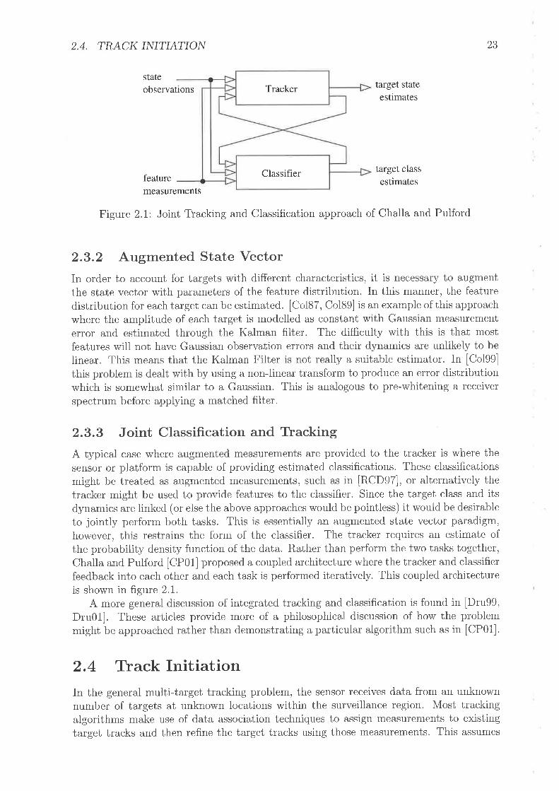
Tracker
Classifier
2.4. TR.ACK INITIATON
stateobservations
feature
23
target stateestimates
target classestimates
measurements
Figure 2.1: Joint Tracking and Classification approach of Challa and Pulford
2.3.2 Augmented State VectorIn order to account for targets with different characteristics, it is necessary to augmentthe state vector with parameters of the feature distribution. In this manner, the featuredistribution for each target can be estimated. [Col87, Col89] is au example of this approachwhere the amplitude of each target is modelled as constant with Gaussian measurementerror and estimated through the Kalman filter. The difficulty with this is that mostfeatures will not have Gaussian observation errors and their dynamics are unlikely to beIinear. This means that the Kalman Filter is not really a suitable estimator. In [Col99]this problem is dealt with by using a non-linear transform to produce an error distributionwhich is somewhat similar to a Gaussian. This is analogous to pre-whitening a receiverspectrum before applying a matched filter.
2.3.3 Joint Classification and TYackingA typical case where augmented measurements are provided to the tracker is where thesensor or platform is capable of providing estimated classifications. These classificationsmight be treated as augmented measurements, such as in [RCD97], or alternatively thetracker might be used to provide features to the classifier. Since the target class and itsdynamics are linked (or else the above approaches would be pointless) it would be desirableto jointly perform both tasks. This is essentially an augmented state vector paradigm,however, this restrains the forrn of the classifier. The tracker requires an estimate ofthe probability density function of the data. Rather than perform the two tasks together,Challa and Pulford ICPO1] proposed a coupled architecture where the tracker and classifierfeedback into each other and each task is performed iteratively. This coupled architectureis shown in figure 2.1.
A more general discussion of integrated tracking and classification is found in [Dru99,Dru01]. These articles provide more of a philosophical discussion of how the problemmight be approached rather than demonstrating a particular algorithm such as in [CP01].
2.4 Track InitiationIn the general multi-target tracking problem, the sensor receives data from an unknownnumber of targets at unknown locations within the surveillance region. Most trackingalgorithms make use of data association techniques to assign measurements to existingtarget tracks and then refine the target tracks using those measurements. This assumes
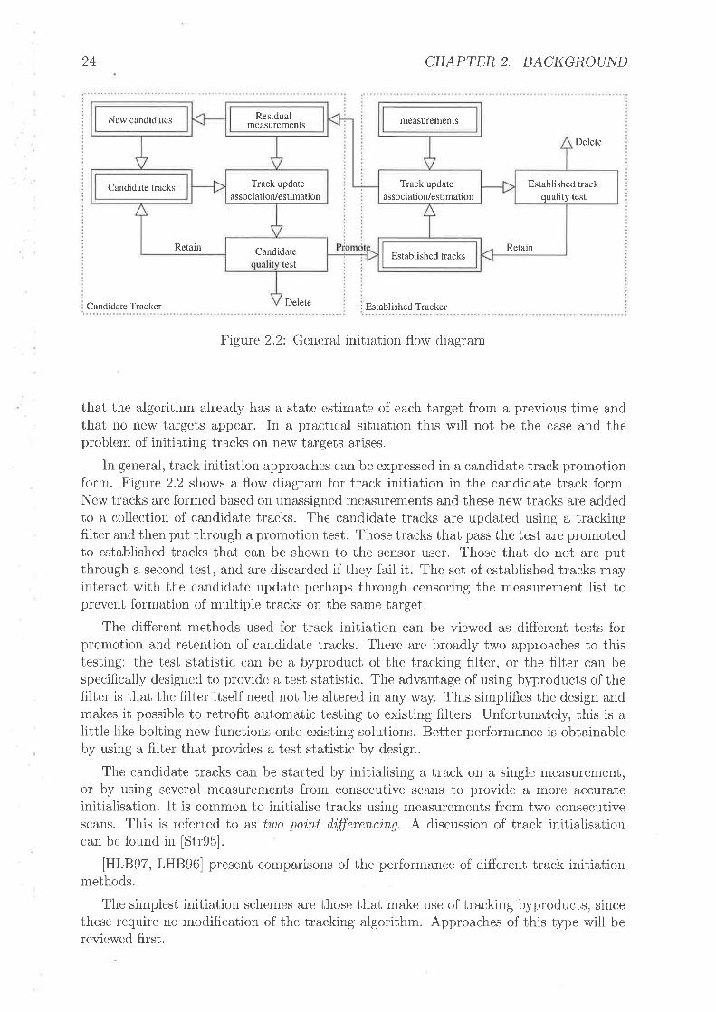
New candidates Residualmeasurements measurements
Candidate tracks Track updateassociation/estimation
Track updateassociation/estimation
Established trackquality test
Retain RetainCandidatetest
Established tracks
24 CHAPTER 2. BACKGROUND
Delete
Candidate Tracke¡ Delete : Established Tracker
Figure 2.2: General initiation flow diagram
that the algorithm already has a state estimate of each target from a previous time andthat no ne'ü/ targets appear. In a practical situation this will not be the case and theproblem of initiating tracks on new targets arises.
In general, track initiation approaches can be expressed in a candidate track promotionform. Figure 2.2 shows a flow diagram for track initiation in the candidate track form.New tracks are formed based on unassigned measurements and these new tracks are addedto a collection of candidate tracks. The candidate tracks are updated using a trackingfilter and then put through a promotion test. Those tracks that pass the test are promotedto established tracks that can be shown to the sensor user. Those that do not are putthrough a second test, and are discarded if they fail it. The set of established tracks mayinteract with the candidate update perhaps through censoring the measurement list toprevent formation of multiple tracks on the same target.
The different methods used for track initiation can be viewed as different tests forpromotion and retention of candidate tracks. There are broadly two approaches to thistesting: the test statistic can be a byproduct of the tracking filter, or the filter can bespecifically designed to provide a test statistic. The advantage of using byproducts of thefilter is that the filter itself need not be altered in any way. This simplifies the design andmakes it possible to retrofit automatic testing to existing filters. Unfortunately, this is alittle like bolting new functions onto existing solutions. Better performance is obtainableby using a filter that provides a test statistic by design.
The candidate tracks can be started by initialising a track on a single measurement,or by using several measurements from consecutive scans to provide a more accurateinitialisation. It is common to initialise tracks using measurements from two consecutivescans. This is referred to as two po'int d'ifferenci,ng. A discussion of track initialisationcan be found in [Str9S].
[HLB97, LHB96] present comparisons of the performance of different track initiationmethods.
The simplest initiation schemes are those that make use of tracking byproducts, sincethese require no modification of the tracking algorithm. Approaches of this type will bereviewed first.
2,4, TRACI< INITIATION 25
2.4.I M of N initiationA comrnonly used test for track initiation is referred to as M of l/ initiation. Under thisrule, candidate tracks must be assigned M rneasurernents in ly' scans. Under low clutterconditions, the rule may require d,[ validated measurements in -ly' scans, a slightly easiercondition. Because the rule is so sirnple, it is possible to generate analytic expressions forquantities such as the probability of prornoting false and valid tracks, which are usefulin quantifying tracking perforrnance [BSCL9O]. A problem with this approach is thatall tracks are quite likely to have validated measurements when the clutter is dense. Inaddition, there is a limited range of promotion thresholds available, since M must be aninteger no more than l/. In order to achieve a very low probability of prornoting falsecandidates, it may be necessary to use a large l/ which delays track initiation.
2.4.2 Accumulated Log-LikelihoodThe first algorithms for track initiation [Sit64] used the measurement innovations to scorethe track. If the target statistics are gaussian, then the sum of the squared innovationsis proportional to the negative of the log likelihood of the measurement sequence. Themeasurement innovations are the difference between the predicted measuretnent and theobserved measurement. When used in a time recursive manner, the squared innovationsare accumulated with time, producing a test statistic proportional to the negative of theaccumulated log-likelihood of the measurements. Valid target tracks are expected to havea low scatter, and the sum of their squared inuovations should be low. False tracks areexpected to give high innovations. This is the same test that is used in the track splitfilter to discard excess tracks. If the target statistics are known (or assumed), then itis possible to determine analytically the probability of observing a particular innovationgiven the measurement is due to the target. This can be used to determine the probabilityof promoting valid tracks for a given threshold on the accumulated innovations [Sit64].
2.4.3 Model Order Estimation Techniques
The track initiation and termination problem is actually a rnodel order estimation prob-lern. This is particularly clear if we view tracking as parameter estimation of a dynamicmixture where the number of components in the mixture is unknown. Methods such as
Maximum Likelihood and Least Squared Error fail in the model order estimation problembecause the model fit to the data can always be improved by added further components.The pioneering work in model order estimation [Aka"74, Sch78, Ris78] resulted in a num-ber of different tests to determine the model order of a data sequence. Of these, theMinimum Description Length (MDL) of [Ris78] is generally accepted to be the best. Thisis because the test due to [Aka7a] is dependent on the number of measurements of thesystem. When more observations are received, it will produce a higher model order esti-mate. Duplicating the data to artiflcially increase the number of measurements producesthe same behaviour. The test due to [Sch7S] has a penalty term that scales with thenumber of measurements, but the MDL also contains a penalty term dependent on themodel complexity (not all order M models are the same).
The MDL test was derived by an information theoretic approach designed to find thestatistical autoregressive moving average (ARMA) model with the minimum number ofcoefficients that fit the observed data. The test chooses the model that maximises the datalikelihood penalised by a term dependent on the model ordel and by a tertn dependent on

26 CHAPTER 2. BACKGROUND
the model complexity. Essentially, a higher order model is accepted only if it increases thelikelihood by more than a prescribed amount. This test can be directly applied to trackinitiation, by promoting candidate tracks only when they sufficiently increase the datalikelihood. An approach analogous to [Sch78] was used in [VLI(00, VL00] to estimatethe number of components in a (static) Gaussian mixture. The technique introduced anew component and used partial trM to optimise the state of the new mixture component.Partial EM updates a subset of the states while keeping the others fixed. The improvementin the EM auxiliary function, namely the increase in the log-likelihood, was tested againsta threshold. This technique could be extended to dynamic mixtures, which is preciselythe EM problem solved by PMHT.
A rnodel order estimation approach such as MDL can be considered as an initiationscheme which uses byproducts of tracking. It is quite similar to the cumulative likelihoodapproach, however it uses the joint likelihood of all tracks, rather than considering eachtrack in isolation. NÍDL requires the rnaximum data likelihood given the model, whichis obtained by using the maximum likelihood estimator for the state. This is what thetracker does anyway, so MDL for tracking can be irnplemented as a candidate test aftertracking, and the tracker is not modified.
2.4.4 Hidden Markov ModelWhen the tracker updates a false candidate track there is a mismatch between the dataand the assumed model. The model assumes that there is a target present that producesa sequence of measurements, when in fact there is none. The initiation methods whichrely on tracker byproducts attempt to detect this mismatch condition and thus rejectfalse candidates. An alternative is to change the model so that it is capable of rnodellingthe false track condition. Candidates would then be accepted or rejected based on theestimated state of the model. This is a fundamentally different approach because it altersthe target state model and integrates the candidate quality estimation with the targetstate estimation.
An extended target state model was first proposed by Colegrove et al in [CDA86].The extended target state contained a binary scoring parameter, referred to as the targetobseruabi,l'ity. The target observability was a first order Markov process that was used tomodel the validity of candidate tracks with the PDA.
The term observability was not adopted by other authors due to the existing statemodelling definition. However, the Markov model for track validity was. In [Col99]Colegrove adopted the alternative term ui,si,bi,li,ty which will be used in this thesis. Thesame approach to initiation with the PDA has been referred to as track eristence in[l\,{ES94] and perce'iuabi,li,ty in lLL01a, LL01b]. This PDA variation is often referred toas the Integrated PDA (IPDA), u term first used by Mu5icki et al. in |N,IES94]. TheMarkov visibility model has also been used with other association algorithms such asin [R400, CVW02]. With this assumed model, there are a number of different possibleapproaches to solve for the probability mass of the target visibility, these will now bediscussed.
2.4.4.I Generalised Pseudo Bayes
The generalised pseudo Bayes (GPB) filtering approach is a fixed lag method for estimat-ing processes with switching modes [Blo8a]. This switching may be in the target model, inthe form of manoeuvre models, or in the form of the visibility model for target existence.
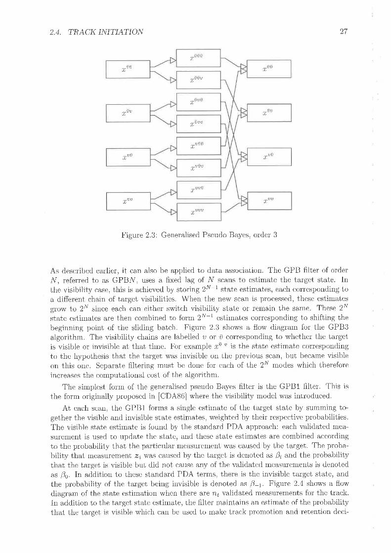
trbuu
Iu1)T,O
Iuuu
:XUUU
ruutruu
ruu't)
ru'úu
luutr'ùu
truuu
:xuuu
truu truu
trDUU
2.4. TR,ACK INITIATION 27
Figure 2.3: Generalised Pseudo Bayes, order 3
As described earlier, it can also be applied to data association. The GPB filter of orderly', referred to as GPB¡/, uses a fixed lag of ly' scans to estimate the target state. Inthe visibility case, this is achieved by storing 2N-1 state estimates, each corresponding toa different chain of target visibilities. When the new scan is processed, these estimatesgrow to 2N since each can either switch visibility state or remain the same. These 2Nstate estimates are then combined to form 2N-1 estimates corresponding to shifting thebeginning point of the sliding batch. Figure 2.3 shows a flow diagram for the GPB3algorithm. The visibility chains are labelled o or Ð corresponding to whether the targetis visible or invisible at that time. For example rù ' is the state estimate correspondingto the hypothesis that the target was invisible on the previous scan, but became visibleon this one. Separate filtering must be done for each of the 2N modes which thereforeincreases the computational cost of the algorithm.
The simplest form of the generalised pseudo Bayes filter is the GPB1 filter. This isthe form originally proposed in [CDA86] where the visibility model was introduced.
At each scan, the GPB1 forms a single estimate of the target state by summing to-gether the visible and invisible state estimates, weighted by their respective probabilities.The visible state estimate is found by the standard PDA approach: each validated mea-surement is used to update the state, and these state estimates are combined accordingto the probability that the particular measurement was caused by the target. The proba-bility that measurement z¡ wàs caused by the target is denoted as Bi and the probabilitythat the target is visible but did not cause any of the validated measurements is denotedàs þo. In addition to these standard PDA terms, there is the invisible target state, andthe probability of the target being invisible is denoted às l3-t Figure 2.4 shows a flowdiagram of the state estimation when there are rz¿ validated measurements for the track.In addition to the target state estimate, the filter maintains an estimate of the probabilitythat the target is visible which can be used to make track promotion and retention deci-
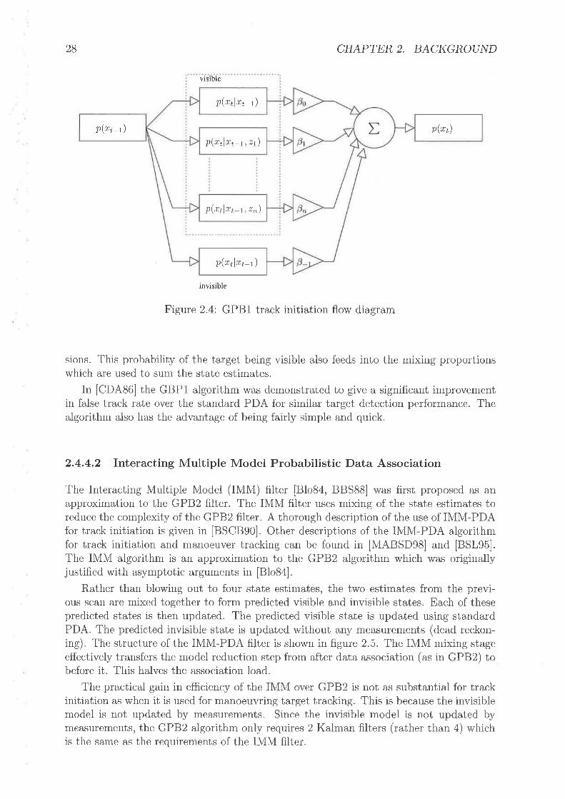
p@tlrr-t)
P(rt_t) p(rt)p(r¡lr;1, z1)
p(r¿lr¡-1, zn)
p(rtlrt-t)
28 CHAPTER 2. BACKGROUND
visible
invisible
Figure 2.4: GPB1 track initiation flow diagram
sions. This probability of the target being visible also feeds into the rnixing proportionswhich are used to sum the state estimates.
In [CDA86] ttre Ceel algorithm was demonstrated to give a significant improvementin false track rate over the standard PDA for similar target detection performance. Thealgorithm also has the advantage of being fairly simple and quick.
2.4.4.2 Interacting Multiple Model Probabilistic Data Association
The Interacting Multiple Model (IMM) filter [BIo84, BBS88] was first proposed as anapproximation to the GPB2 filter. The IMM filter uses mixing of the state estimates toreduce the complexity of the GPB2 filter. A thorough description of the use of IMM-PDAfor track initiation is given in [BSCB9O]. Other descriptions of the IMM-PDA algorithmfor track initiation and manoeuver tracking can be found in [\tIABSD98] and [BSL95].The IMM algorithm is an approximation to the GPB2 algorithm which was originallyjustified with asymptotic arguments in [Blo84].
Rather than blowing out to four state estimates, the two estimates from the previ-ous scan are mixed together to form predicted visibie and invisible states. Each of thesepredicted states is then updated. The predicted visible state is updated using standardPDA. The predicted invisible state is updated without any measurements (dead reckon-ing). The structure of the IMM-PDA filter is shown in figure 2.5. The IMM mixing stageeffectively transfers the model reduction step from after data association (as in GPB2) tobefore it. This halves the association load.
The practical gain in efficiency of the IMM over GPB2 is not as substantial for trackinitiation as when it is used for manoeuvring target tracking. This is because the invisiblemodel is not updated by measurements. Since the invisible model is not updated bymeasurements, the GPB2 algorithm only requires 2 Kalman filters (rather than 4) whichis the same as the requirements of the IMM filter.

p(ni.l",-t)
p(""r)p@i-') p(ni@t-t)(rfln¿-1, z1
r?lrt-r,
p(ri.-) p(nilnr-t) p(rilrt-t) p(rI)
2.4. TR.ACI< INITIATION 29
visibte
invisible
Figure 2.5: IMM flow diagram
2.4.4.3 Integrated Probabilistic Data Association
A slightly different approach is termed Integrated Probabilistic Data Association (IPDA)[\4ES94]. The GPB and IMM approaches both formed the mean and covariance of thetarget state over both the invisible and visible models. Instead, the IPDA calculates theconditional mean and covariance of the target state, given that it is visible. If the invisiblemodel is chosen to be absorbing (i.e. a track can never change to visible from invisible)then the conditional pdf of the target state depends only on one sequence of the Markovchain, namely the target being visible for all scans. Thus, when the invisible model isabsorbing, the conditional state distribution can be estimated using a normal PDAF. Theonly extra requirement is to calculate the visibility probability.
The IPDA approach is potentially limiting, since it inherently specifies the invisiblemodel to be absorbing, but the conditional state estimate should give better estimationaccuracy than the GPB unconditional one, because the latter damps the filter gain basedon the visibility probability. In [LL01a] a formulation of both types of algorithrn ispresented. Theoretical and simulated comparisons conclude that the GPB1 algorithmhas slightly poorer error statistics, but confirms slightly fewer false tracks than the IPDAalgorithm. Overall, the differences are minimal. [l\,iEsg4] gives a comparison of IPDAand IMM-PDA where the two algorithms give almost identical performance. [LL01a] alsoconcludes that the added complexity of the IMM algorithm does not provide a performanceadvantage for initiation.
2.4.5 Radon and Hough TlansformsThe optimal strategy to detect a target would be to coherently integrate all of the energythat the sensor received from it to maximise the detector SNR. The difficulty with thisis that we do not know the target trajectory. It is not feasible to test all conceivabletrajectories, since there will be an infinite number of them (or at least a very largequantity). However, the Radon transforrn can be used to test all possible linear trajectoriesthrough the data. The Radon transform is a mapping from the position space into aparameterised line space. Peaks in the Radon space can be used to detect straight lines inposition space. Usually the discrete version, referred to as the Hough transform lDH72,IK88] is used to detect lines in images. The Hough transform has been applied to detection

30 CHAPTER 2. BACKGROUND
and tracking for radar in [CEW94a, CEW94b, CEW94c] and more recently it has beenintegrated into the PMHT framework in [LSW01]. A drawback of this approach is that ituses the full data a,rra,y received by the sensor and requires a number of scans of the samespatial region, This may result in a large memory requirement for a stepped scan sensor.

Chapter 3
Multi-Target Problem Formulation
rf'lHIS chapter defines the multi-target tracking problem in clutter and introduces the sta-I tistical framework that shall be used in the following chapters. It follows the method
used by Streit and Luginbuhl in [SL95] to derive the Probabilistic Multi-HypothesisTracker. However, the same framework can also be used to derive other algorithrns suchas the Probabilistic Data Association Filter. The concept of the observer is reviewed, andthe structure of the observer for the case of multi-target tracking in clutter is presented.Particular state models of interest are presented.
The standard PMHT algorithm is then stated, and sorne of the existing enhancementsto it are discussed. Areas where the PMHT may be improved are highlighted, in particularthose addressed in later chapters of this thesis.
3.1 Problem DefinitionSuppose that a sensor observes a particular surveillance region and reports measurementsat irregular intervals, referred to as scans. At each scan, there are multiple measurements.Some of these measurements are caused by signals that are of interest to the sensoroperator, and are referred to as target detections. The other measurements may becaused by various undesired interference and noise processes collectively referred to as
clutter. LeT Z denote the collection of all measurements from the sensor over a batchfrom scan 1 to scan T . Let r¿ denote the time at which scan ú was collected and n¿ denotetlre number of measurements formed by the sensor in scan ú. Assume that r¿+r ) r¡ forall ú. This merely implies that the measurements are ordered in time sequence and thatall measurements observed at a particular time are collated in a single scan. Although itis possible to consider a more general problem, where measurements are received possiblyout of sequence, this is beyond the scope of this thesis. Define Z¡ to be the vector of allrneasurements in scan ú.
Zt : lzu,zt2,...,zmrf, (3.1)
where z¡, is tlrc r'th measurement in scan ú. The set of all measurements Z can be writtenas the set of the per scan vectors Z¡.
Z:{Zt,Zz,...,Zr}. (32)
The probabitity density of the measurements, P(Z), is a mixture of the measurementprobability densities due to each of the various sources in the sensor scene, that is, P(Z) isthe weighted sum of the measurement probability densities of the sources. The weighting
31

32 CHAPTER 3. AIULTI-TARGET PROBLEM FORMULATION
for each source is referred to as the mixing proportion for that source and the measurementprobability for that source is a component of the probability density function oT Z. Each ofthe source measurernent probability densities has a known functional form with unknowntime varying parameters, called the state. The goal is to find the dynamic mixture modelthat best describes the probability density function of the measurements Z, namely thestates that maximise the probability of the observed measurements. This is a lVlaximumLikelihood Criterion for estirrating the states.
3.2 The ObserverThe PMHT observer as introduced by Streit and Luginbuhl in [SL95] consists of twoparts. Firstly, there is a collection of continuous states. These states are the dynamicparameters of the components of the measurement mixture density function. Secondly,there is a set of discrete assignments. These assignments label the true source of everymeasurement in the set Z.
The continuous state part of the observer is composed of a number of models. Eachmodel is used to represent an independent source of sensor measurements. Let the numberof target models be My and the number of clutter models be My. The total number ofdynamic state models is
M:MxlMv. (33)
The distinction between target and clutter models is unnecessary at this stage sinceboth are simply members of the dynamic mixture. The PMHT algorithm is not tied toany specific models for target or clutter behaviour. Instead, models are specified based onthe problem at hand, and a particular solution is achieved for those models. The modelsdo not have to occupy the same state space, and it is likely that it will be useful to havedifferent state vectors for different models. For example, the state representation of clutterprocesses will most likely be different to the state representation of target processes. Itis assumed that the dimension of the state vector for each model does not vary over thebatch.
Let æi deuote the state of model m at time r¿ corr€sponding to scan ú. Supposethere is some time rs at which the probability density function of the state æff is known.In a practical system, this density function may not be known and track initialisationtechniques would be used to estimate it.
Define the temporal collection of model states over the batch for model zn as
X-: l*i,*T,...,æil.The total collection of all states is defined as
x: [x',X',...,Xt] ,
and the vector of all states at a particular scan is denoted
X,: l*I,n?,. . .,*yl .
(3.4)
(3 5)
(3 6)
Denote the (known) probability density function of the state of model m at time roàs 1þi @T) Assume that the evolution of the state of model m is a first order Markovprocess. That is, given the state of the model at the previous scan ælr, the state of themodel at the current scan æl is conditionally independent of all prior states æi ...æ72.

3.2. THE OBSERVER.).)JÙ
Denote tlre (known) probability density function of the state evolution as ,þ7 (*Tl*?t)This function is implicitly dependent on the time elapsed between scans ú and f - 1, i.e.
Tt - Tt-t.The observer also contains the assignment of each. measurement to the model that
caused it. For the rth measurement,, z¡r, at scan ú there is a corresponding assignmentindex, k¿r, thal denotes the model that gave rise to that measurement. The assignmentindex is an integer in the range lI, M| When the assignment index k¿" takes a value inthe range lI,M"l then this indicates that measurement z¡ywàs caused by clutter modelkr,. When it takes a value in the range lMn + I, Mx ¡ Mv) then this indicates thatmeasuremettl z¡, was caused by target model k¿". Define the set of all assignment indicesat scan f as
Kt = lkrr,krr,... ,krnr],
and the set of assignment indices over the whole batch as
K:[Ko,Kr,...,Kr] ,
(3 7)
(3 8)
where Ko : Ø, i.e. the empty set, because there are no measurements at time r¡.Notice that by defining the association indices K there is an implicit assumption that
each measurement is caused by only one of the models. There is no allowance made forthe possibility that more than one model might contribute to a measurement, for examplethe case of two closely spaced targets that are not resolved by the finite aperture of aradar.
The observer at scan ú is then defined as the combination of the model states and theassignment indices for scan t at' time r¿:
O¿ : {X¿, K¿} , (3.9)
and the batch observer is defined as the collection of model states and assignment indicesover the entire batch:
O: {X,K}: [Oo,Or.,...,Or] . (3.10)
3.2.L The Assignment ModelUnder the standard assignment model for tracking, each target is able to form, at most,one mea,surement. It is assumed that the sensor uses a detection process that may notalways form a measuïement when a target is present. This missed detection may be due
to random signal fluctuations, environmental factors, or simply low signal strength at thedetector. When the target is detected, it may be distributed through several sensor cells,
however the detector is assumed to produce a single measurement from these distributedreturns. Each target thus produces either no measurement or exactly one measurement.This implies that no two assignment indices, for different measurements in the same scan,
can indicate the same target model. That is, the number of indices which take the valuem e Mv , . . M is either zero or one. Mathematically this is represented as:
nt
Ðd(rr,-rn)e{0,1} Mvtllm<M, (3.11)r:7
where ð(.) is the Dirac delta, an indicator function that is unity at the origin and zeroelsewhere. There is no constraint on the number of measurements assigned to the clutterrnodels.

34 CHAPTER 3. MULTI.TARGET PROBLEM FORMULATION
The constraints (3.11) cause the assignment problem to be difficult to solve and resultin algorithms with greater than linear complexity in the number of measurements. Thisconstrained assignment model is used in the Probabilistic Data Association Filter and theMulti-Hypothesis Tracker.
In the PMHT, the assignrnents are assumed to be independent identically distributedrandom variables. This assumption conflicts with the constrained assignments used forPDAF and MHT. Because PMHT uses this assumption, it allows each target to producemore than one measurement, and the constraint 3.11 can be violated. Letri denote theprobability that the assignment index k¿¡, corresponding to the rth measurement at scanú, takes the value rn. Since Lhe k¡, are identically distributed, rl is the same for aII r (ris an arbitrary indexing). Define the following sets of rf:
fI¿= 1"1,"?,...,ny1 ,
il : [IIr, fI2,. .. , flr] .
3.2.2 The Measurement Process
e| (r*l*i)
e? Q,,l*?)p (zt lXr, kr") :
In addition to the observer, a measurement process is used to link the states and theassignments with the received measurements. The measurement process for each modeldefines the probability density function of measurements from that model over the surveil-Iance region. The measurement processes are each functions only of the state of thecorrespouding models. All measurements are assumed to be independent identically dis-tributed random variables drawn from the measurement probability density for the modelgiven by the assignment index corresponding to the measurement. This means that themeasurement process is a mixture process and the unconditional probability density ofthe measurements is a weighted sum of the individual model measurement densities.
Different models may have different measurement processes (indeed they must if themodels have different state vectors). The measurement probability density function formodel m at scan ú is denotedbV eT Ql*T). Note that it has also been implicitly assumedthat the measurements at scan ú are independent of the states at all other scans whenconditioned on the states at scan ú. The independence of rneasurernents conditioned onthe model states is a common assumption to tracking algorithms. The probability densityfunction of measurement z¡, is then:
(3.r2)
(3 13)
(3.14)
if kr,:1
tf kr,:2
elo (r*l*Y) ,f k,,: M
3.3 Target and Measurement ModelsUp to this stage, the tracking problem has been defined using completely general formsfor the probability density functions of the target state evolution and the measurementprocess. Without specifying these processes in terms of statistical rnodels, it is difficultto proceed to a solution for the estimation of their parameters.
3.3. TARGET A¡\ID MEASURÐMENT MODELS 35
One commorÌ assumption in marìy tracking applications is that of linear Gaussianstatistics. A reason for the popularity of this model is that the probability density functioncan be defined using a frnite palameter set, namely the mean vector and covariance matrix.Further, the solution to the estimation problem is well known for linear Gaussian statistics.That is, given a set of rneasurements, it is possible to find the optimal state estimate. Theclosed form solutiorr for this estimate is the Kalman smoother. The state evolution andmeasuïerlent models are now examined in more detail, presenting the linear Gaussianforms frequently used.
3.3.1 State Evolution ModelRecall that the target evolution is assumed to be a first order Markov process. Therefore,the most general form of the evolution can be written as
æT : fT (*7,,,uT,uT), (3.15)
where ui ís a control input, ui is random noise (referred to as the process noise), and
fTO issomefunction. Inthetargettracking case,n! generallyrepresentsthedynamicstate of a non-cooperative target (perhaps with other non-kinematic attributes), so it is
necessary to concede at this point that the control input ui is unknown and it will becompensated for by using an artificially inflated noise process. Under the assumption ofadditive noise, the state model can be rewritten as
æT : rT @7,) + gT @T), (3.16)
where the functions /i(.) and gfl(.) are arbitrary, and perhaps nonlinear. In manypractical applications, such as the tracking of ballistic objects ICKBSOI, YBSPD9S], it isnecessaïy to use nonlinear functions for fi(.) and gi"(.). Nevertheless, in other cases, itis more usual to assume that they are both linear, and further that the noise process trfis Gaussian. This allows the use of the Kalman Filter for state estimation, whereas thenonlinear, non Gaussian case requires an approach such as particle filtering.
Under the linear Gaussian model, the evolution density of the target state is a linearfunction of the target state at the previous scan corrupted with Gaussian noise. The stateevolution is thus represented by
æT : FT*\r-t Giai, (3'17)
where ui is a zero mean Gaussian random vector with covariance Qf and Fi" and Giare appropriately sized matrices. Equation (3.17) is a general linear state model withadditive noise. In the tracking application, the matrices Fl", Gfl and Qi" are determinedby the equations of motion and the motion model used. For example, a common modelis the almost constant ueloci,ty model. Here, the target velocity is assumed to be constantexcept for accelerations introduced by the noise process, ul. For a one dimensional almostconstant velocity model, the state vector consists of one dimensional position and velocitv,
æi$D) :[;]
(3.18)
the process noise covariance , QT, is a scalar, and so:
I r¡ - r¡_101Fr(lD) : (3.1e)

36 CHAPTER 3. MULTI-TARGET PROBLEM FORMULATION
Gr(lD) :fåt:-:ì'l (320)L rt-rt-t I
The almost constant velocity model at higher dimensions can be composed simplyfrom the matrices Ff(1D) and Gfl(1D). For exarnple, for a three dimensional model Qiis a 3x3 symmetric positive definite tnatrix and:
Fr(3D) : Fr(lD) o o0 Fr(1D) 0o o Fr(1D)
Gr(lD) o oo Gr(lD) oo o Gr(lD)
(3 21)
(3.22)
assuming that the random variations in speed are independent for each velocity compo-nent.
Using (3.17) it is straightforward to show that the covariance of æi given æp, isGTQTGT'. It is clear from (3.20) that this covariance of the state evolution is singular.That is,
,u,* {ø løf - FT*T,) @T - rf *7,)'f} : 'u,.u {af } < dim {*T}. (3.23)
This is because the only random elements are the velocity perturbations and there isno random fluctuation of the position, except as an integration of the velocity. This meansthat the probability density function of the state evolution exists only on a manifold and iszero elsewhere. The position is completely dependent on the velocity fluctuations. Whilethis is unimportant for Kalman Filtering (since the Kalman Filter does not require thisinverse) it is important to recognise this in order to write down the proper expression forthe evolution density, lþT (*Tl*pr). The only time that the evolution density is requiredis in the calculation of the PMHT auxiliary function that is used to test convergence. Sincethe random part of the evolution comes through the noise process, u!, the probabilityevolution density is simply the noise probability density. Under the almost constantvelocity model, the process noise produces a deviation in the velocity, so the differencebetween the target velocity at ri and ú - 1 determines the value of the noise, of .
So the state evolution probability density is given by
,þT (*Tl*7,) : lzne1l-å ."p {_.iO, - *7,)'A'ef-'A (*T -rf ,)} , e.24))
where the matrix A is used to pick out the velocity cornponent of the state, for example
(3DGT
A(3D) : (3.25)
This pdf applies provided the position deviation matches the velocity deviation, otherwisethe probability of the state transition is zero.
In addition to the evolution probability density, the estimator requires the initialprobability density function of the model states, ,þi @T). In general, this function mighttake any form, but under the assumption of linear Gaussian statistics, ,þi @T) is also aGaussian function. Let the mean and variance of æff be æff and Pfi' respectively. Theinitial state distribution is thus:
,t,i @Ð : l2npffl-' "*o { -f,f*f - æi)'pi-'@i -.n} (3.26)
lo 1 o o olo o o 1olo o o o o il

3.3. TARGET A¡\ID MEASUREMENT MODELS ùt
3.3.2 Measurement ModelRecall that there is a measurement probability density for each model, namely CT QI*T)In general, this density is the result of the nonlinear measurement process
ztr: hT @T,urtr), Q.27)
where tlre source of measurement z¡, is model m as defined by the index k¿r, and ulis random noise. Under the assumption of additive noise, and assuming that the noisevector, r.t)¡r,has the same dimension as the measurement vectot, z¡r, (3.27) becomes
Ztr : nT @T) t u)u. (3.28)
In almost all tracking applications, the true measurernent equation is nonlinear, be-cause the seusor receives observations in a polar coordinate system (such as range, bearingand elevation) but the target state is represented in a Cartesian coordinate system (alti-tude, north, east) or in a geocentric coordinate system (altitude, Iatitude, Iongitude). Ifthe target state is modelled in the radar polar coordinate system, then the state evolutionwill be nonlinear (since targets do not move at constant range or azimuth rate except inspecial cases). When the target state occupies a Cartesian coordinate system, and thesensor measurements are in a polar coordinate system, the bearing measurement functionbecorrres an arctangent.
The modelling method for the measurement process depends very much on the degreeof nonlinearity. For active sensors that operate at very long range, it is reasonable toassume that targets move at constant velocity in the radar polar coordinates. This makeslife simpler, since the whole problem now becomes linear. This approach is appropriatefor sensors such as Over the Horizon Radar which typically operate at ranges greaterthan 1000 km. At intermediate ranges, the nonlinearity cannot be ignored, but it is stillnot a large problem. Sensors such as active microwave radars typically use a first orderTaylor approximation to the nonlinear function, namely the extended Kalman Filter. Atclose range, or with passive sensors where a range measurement is unavailable, it becomesnecessaïy to use a nonlinear filter such as the particle filter |DDFGOI].
Since the following analysis will be mainly concerned with association performance,and not estimation performance, it is possible restrict the problem to linear measurementmodels, These models are also appropriate for the physical application which will beexplored later, namely Over the Horizon Radar.
The linear Gaussian measurement model replaces (3.28) with
ztu : HT*T I urt,, (3.29)
where Hi is an appropriately sized matrix, and ra¿, is zero mean Gaussian noise withcovariance matrix Rl".
Under the linear Gaussian measurement model, the measurement probability densityfunction is then given by:
: l2nRil-å "*p {-io" - HT *T)'RT_' (.,, - HT æn\ . (3 30)
A cornmonty a'alysed probtem is where the measur;";. """t;" ""r', *."r"",,"",of the target position. For the almost constant velocity target model, this corresponds to:
Hr(lD) : [1 o] . (3.31)
38 CHAPTER 3. MULTI-TARGET PROBLEM FORMULATION
In a similar manner to the matrices Fi and Gfl, the meâsurement matrix for higherdirnensional problems can be expressed in terms of the one dimensional measurementmatrix. For example,
Hr(3D) : U
Hr(1D)0 rn
tH
(1D)00
HT 00(
(3.32)1D
3.4 The Kalman FilterWhen the evolution and measurement processes are linear and the random elements areGaussian, then the probability density function of the model state, given a collection ofobservations of that model, is also Gaussian. So, the posterior state pdf can be fullydescribed by its mean and variance. The Kalman Filter is an optimal recursive estimatorfor the mean and variance of the posterior state pdf. It provides a method for calculatingthe mean and variance based on their values at the previous scan and on the m.easurementobserved at the current scan. The Kalman Filter is analysed in detail in many texts (e.g.
[CC99]) and will not be reviewed in detail here. However, it is a fundamental buildingblock of most tracking algorithms, in particular the Probabilistic Data Association Filterand Probabilistic Multi-Hypothesis Tracker. For this reason, the Kalman Filter equationsare nov¡ briefly reviewed.
Suppose, at scan t - I, the mean and variance of the posterior state pdf are known.Let these be denoted as:
ùT-t: E{*7tlZr,...,Zr-r}, (3.33)
P7, : cov {æirlZr,...,Zr-r} , (3 34)
where both (3.33) and (3.34) are implicitly dependent on the known prior distribution ofthe state, ,þi @T)
At scan ú, the measurement z¿^ is received. It is assumed to be known that therr¿th measurement is due to model m. The new mean and variance of the state pdf arecalculated using a two step procedure. Firstly, the mean and variance are predicted basedon the previous data, this is referred to as the prediction step. In the correction step (alsoreferred to as the filtering or update step) , the predicted quantities are adjusted usingthe received measurement.
The prediction step extrapolates the state mean and covariance using the followingequations:
ûir-t : FTùT-t, (3.35)
Pi,-r: FTPTÏTr+GTQTGTT. (3.36)
The prediction step also calculates the mean and the covariance of the measurementz¿q, àI scan ú, conditioned on the predicted state and its associated error covariance. Themean of the conditional measurement pdf (i.e. the expected measurement) is given by
2T : HTûft-r' (3'37)
(3.38)and its covariance is
si:HTPit-tHir+Rfl

3.4, THE KALMAN FILTER 39
This concludes the prediction step. The correction step adjusts the predicted statestatistics from the new measurement, z¡^. In the correction step, the filter calculatesthe measurement tnnouat'ion. The innovation is defined as the difference between theexpected measurement and the actual observed measurement, and is denoted zj':
uT : zr- - 27. (3.39)
Note that the innovation has à zero vector mean, because 2i is defined as the meanof z¡^, provided the initialisation is unbiased. Also, the covariance of the innovation is
the covariance of the conditional measurement pdf, namely Si. Hence, S|' is referred toas the innovation covariance matrix. This matrix is very important because it controlsthe gain of the filter.
Next, the Kalman gain, Wfl, is calculated using
wT : Pir-iH1rs1-'. (3.40)
The correction step then concludes by forming the new state mean and covariance:
æf : ûir-r-tWiui, (3'41)
PT : PT,_, - WrHTPft4. Q.42)
Notice that the Kalman gain and the state covariance do not depend on the actualmeasurements received. This means that these quantities could be pre-computed if thematrices FT, GY and Hi are known a priori. In practice, both Fi and Gf depend onthe difference between consecutive scan times. So, if the scan rate is constant (or variesin a known predictable way) then Fi and Gfl can be known a priori and the gains andcovariances computed off line. For many sensors this will not be the case, since the scanrate may fluctuate.
The Kalman Filter can be presented in different formats. In particular, it is possibleto write the whole filter as two equations, one for the mean and one for the covariance.However, this format has been chosen because data association at scan ú will be performedusing the predicted measurement, (3.37).
3.4.L The Kalman SmootherThe Kalman Filter is used to estimate the state in a time recursive manner, howeverin some applications the estimator has access to a batch of data. In this case, futuremeasurements can be used to improve the state estimate at scan ú. The Kalman filter canbe extended to handle batch data, and this extension is called the Kalman Smoother.
The Kalman Smoother is almost identical to the Kalman Filter, but it involves anextra correction step after the filter has calculated the recursive state estimates for thebatch. Define the smoothed state mean and covariance as:
ñi, : n{rilz}, (3.43)
Pi, : cov {rilz} . (3.44)
The state mean and covariance at the final scan 7 are already conditioned on thewhole batch, so
ûiv (3.45)fti,Pi.PTv (3.46)
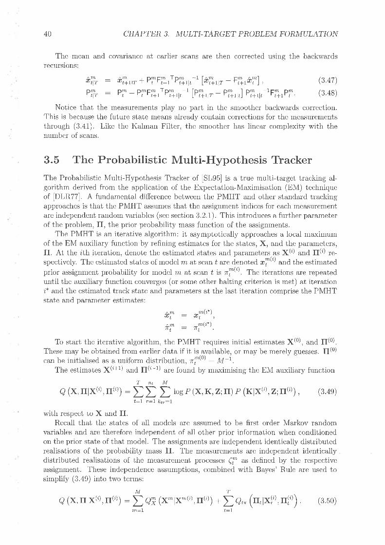
40 CHAPTER 3. MULTI-TARGET PROBLEM FORMULATTON
The mean and covariance at earlier scans are then corrected using the backwardsTECUISlONS
ûi, : ûT*r¡r + PTFnIrP\*r,'-t lûtT*rlr - FT*rùT) , Q.47)ph : pT +plFntlpn,¡t-l fpär¡r - pärl,] pT*r -',Fr *,,pT. (3.48)
Notice that the measurements play no part in the smoother backwards correction.This is because the future state means already contain corrections for the measurementsthrough (3.41). Like the Kalman Filter, the smoother has linear complexity with thenumber of scans.
3.5 The Probabilistic Multi-Hypothesis TrackerThe Probabilistic Multi-Hypothesis Tracker of lSL95] is a true multi-target tracking al-gorithm derived from the application of the Expectation-Maximisation (EM) techniqueof [DLR77]. A fundamental difference between the PMHT and other standard trackingapproaches is that the PMHT assumes that the assignment indices for each rneasurementare independent random variables (see section 3.2.1). This introduces a further parameterof the problem, fI, the prior probability mass function of the assignments.
The PMHT is an iterative algorithm: it asymptotically approaches a local maximumof the EM auxiliary function by refining estimates for the states, X, and the parameters,II. At the zth iteration, denote the estimated states and parameters as X(i) and ¡(l) t"-spectively. The estimated states of model m at scan ú are denot ed, æi@ and the estimatedprior assignment probability for model m at scan t is riØ. The iterations are repeateduntil the auxiliary function converges (or some other halting criterion is met) at iteration¿* and the estimated track state and parameters at the last iteration comprise the PMHTstate and parameter estimates:
ùT : æ!(i.) 'îT : ni?-l '
To start the iterative algorithm, the PMHT requires initial estimates [(0), ¿nfl fl(O).These may be obtained frorn earlier data if it is available, or may be rnerely guesses. fI(O)can be initialised as a uniform distribution, zf(O) : M-|.
The estimu¡.r ¡(z+t) and II('z+1) are found by maximising the EM auxiliary functionTntM
Ç (x,illx{r), rl(n)) : t t t log P (X, K, z;n) P (Klx{t) ,z;rr?')¡, (3.4e)t:I r-I let":I
with respect to X and fLRecall that the states of all models are assumed to be first order Markov random
variables and are therefore independent of all other prior information when conditionedon the prior state of that model. The assignments are independent identically distributedrealisations of the probability mass II. The measurements are independent identicallydistributed realisations of the measurement processes (fl as defined by the respectiveassignment. These independence assumptions, combined with Bayes' Rule are used tosimplify (3.49) into two terms:
MTg (x,rlx(r), rr(n)) : t eT (x^lx-tz), rr(o)) + t e,- (n,1xÍn), iljn)) . (3.b0)
1n:l t:l

3.5. THE PROBABILISTIC MULTI-HYPOTHESIS TRACKER 4L
8r, (n,¡Xio),ilt0,) rnust be maximised subject to the constraint th.t t rT:I,namely II¿ should be a proper probability vector. This is achieved fry in#ãta,tcing a
Lagrangian multiplier and the resulting solution is
m.(¡.\1Tt " .n,, (3.51)
wlrere ,flr, i" referred to as the assignment we'ight for measurement z¡y and. model m.This weight can be interpreted as the posterior probability that measurement z¡, is d:ue
to model m. It is given by:
( i.\urn't
riu) * ("*l*Tto'(3,52)
From (3.52), it can be seen that the weight, ,9r,, captures the dependence upon thestate and parameter estimates from the previous iteration.
Theterm Q^(X 1X(¿),fl(i)) in(3.50) isafunctionof thestatesof targetrnoverthebatch and is independent of the other models. This implies that the state estimation formodel m is independent of the state estimation of the other models. This term is givenby,
Q* (x*]x-('),If(l)) :TTTLT
roe,þi @Ð +D.* ,þT @Tl*7,) * i t,l|,,rosef Q,,l*T), (3'53)
t--1, t:l r:1The weight equation (3.52) has a linear complexity in the number of models and the
models are maximised independently, so the overall PMHT complexity is linear with thenumber of models.
The state estimate for model m at iteration z, ¡nz(í+l), is that state sequence thatmaximises Q^ (X^1X(i),fl(i)). This is a maximum likelihood problem with weightedmeasurements. The objective likelihood function (3.53) is the same as the likelihoodfunction of an unambiguous measurement problem, except for the measurement term.The unambiguous measurement case is maximised by the Kalman Smoother when thereare linear Gaussian statistics. For linear Gaussian statistics, (3.53) becomes
T
Q^ (x^1x-(¿), rr(i)) : IoB ,þi @i) + t toerþT @Tl*7) + c* +t:7
T n¿ _ _.,,(i)t t ff1r,, _ HT*T).RT-' (.r, _ HT*Ð, (3.54)t:I r:7
where C^ ís a constant factor due to the measurement density normalisation.Through algebraic manipulation, (3.54) can be rewritten as
T
Q^ (x^ l>c-{';), fl(n)) :roeúi (rä') + I to* ,þT @Tl*Ï-') + c^ +t:1
nt
Tr:l
M
D ^f(o)C," ("* *í'o')
s:1
_1TL¡
Tt 1
t:l 2(rT,, - HT*T)' (n¡r'r¡-' çry,, - HT*T), (3 bb)

42
and
CHAPTER 3. MULTT-TARGÐT PROBLEM FORMULATION
where
rn(i\TLtTlt '(3 56)
i)- 1
m(i\TLtTft 'Rr
The likelihood function in (3.55) is the same as the likelitrood function optimised bythe Kalman smoother. However, instead of the measurement probability density for modelm, e? Q*l*T), a modified measurement density with covariance Rf(" appears. The mea-surement centroid, ZT@ , acts as a synthetic measurement. So, the model state estimate,æl(t), can be found using a Kalman Smoother where the measurement probability densityis given by
(3.58)The term 8r, (n,¡xjo),ilj')) in (3.50) is a function of the parameter vector fI¿ and
is independent of the parameters at other scans and independent of the model states. Itis given by
M
O,* (n,¡xio',do') : t wflr,Iogri. (3.5e)m:1
The PMHT algorithm is then the repeated application of equations (3.52) and (3.51)along with Kalman smoothing to estimate the model states. At each iteration, the statesand parameters are modified and this produces new weights through (3.52). When thealgorithm converges) the changes in the estimates and weights will become small.
It is important to recognise that the weight equation (3.52) uses the measurementprobability density ei Qt læi), which is the probability density of the measurementswhen the model state is known. This is different from the PDAF which uses the probabilitydensity of measurements conditioned on the current state estimate (and its covariance).
3.5.1 Homothetic Measurement ModelsAn irnportant extension of the PMHT is the introduction of homothetic measurementmodels [RWS95a], The homothetic measurement model replaces the simple Gaussianmodel lor Çi Qr,l*T). Rather than a single Gaussian, the homothetic PMHT uses aGaussian mixture where each of the components has the same mean, but different covari-ance matrices. In published uses of the homothetic model, the covariance of each of thecomponents is a scalar multiple of the measurement variance. It is possible to use a moregeneral form of the homothetic model, and this is presented in chapter 6.
The homothetic mixture model comprises of P Gaussian components, each with meanHTæT, and with covariance rc*pR! , where n^p is a scalar. Chapter 6 uses a more generalmodel where the covariances of the different components are arbitrary time varying ma-trices. Since the measurement process for each target is now a mixture, the index variablek¿" must assign measurements to both the appropriate model and the homothetic mixturecomponent of that model's measurement process. So the new assignment index is
ler,:{tl,,tt|}, (3.60)
-m.(i.\z¿1
D'9,.'n,r:l
ñr(
Ç (uTu'*r) 2na7Ø -åexp {-iGr") -HT*T)'(nft";-',
(3.57)
- rn( T*THi)
))

3,5, THE PROBABILISTIC MULTI-HYPOTHESIS TRACKER 43
where kl, e lI,M] indicates the state model that corresponds to the true source of mea-surement z¡y, àr1d k!, e lI,P] indicates the homothetic mixture component of that modelthat caused the rneasurement.
The homothetic mixture model for the measurement process for model rn then gives
the measurement density:
e?'Q"l*T)
CT'Q*l*T)
ir kl,:1tf kl,:2
Ç ("r,1*T) : (3.61)
ei" ("*l*Y) lf kl,: P,
where
eT' Q*l*T) : l2trn^PRil-å ""p -!r{rr, - HT*T)- @*eRi)-I (tr, - Hf *T)}(3.62)
There is now a different assignment weight for each homothetic component, since theyrepresent different measurement pdfs. These weights are given by
(L)Umptr
ri(ù ,* @) eT' (r*l*T'u')(3.63)
Ð"',(o) PIi @) ein (.*l*it'')
where p# (p) is the prior probability mass of the index kl, lor model m, i.e. the mixingproportions for the components of the measurement density for that model. In [RWS95a,RWS95b], this mass was implicitly assumed to be known to be uniform. However, it maybe desirable to assume a nonuniform probability mass, or adapt it with the data. If it isassumed unknown, then the probability mass Pffi (p) can be estimated in the same wayas the probability mass fL
Under this new measurement model, the assignment prior is then estimated by
(3.64)
If the homothetic model prior is to be estimated, then it is given by
p^1(u) (p) :D'9,"r:l (3 65)ntPtt'f)*,
r:1 s:1
tvltS:1
P
a:I
11. I
Umptr.ntPnTu):lYY' nr ¿-t ¿-¿" r:I p:I
The target state estimates can still be derived by a Kalman Smoother with syntheticmeasurements and covariances defrned by
2T(,:{åå%) 'Ë E_%,).,,, (366)
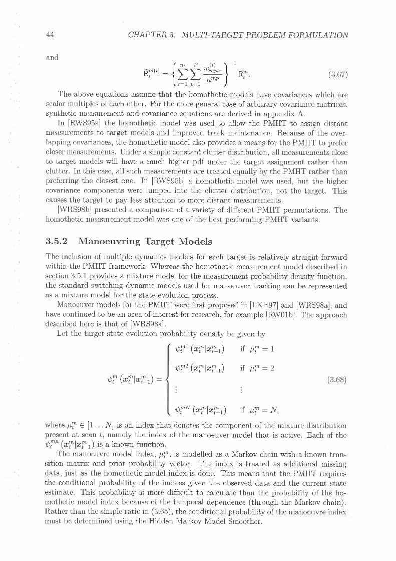
44
and
CHAPTER 3. MULTI-TARGET PROBLEM FORMULATION
ñirtr - tt .9rn -1PntRr (3.67)
K,mPr:l p:lThe above equations assume that the homothetic models have covariances which are
scalar multiples of each other. For the more general case of arbitrary covariance matrices,synthetic measurement and covariance equations are derived in appendix A.
In [R\VS95a] the homothetic model was used to allow the PMHT to assign distantmeasurements to target models and improved track maintenance. Because of the over-lapping covariances, the homothetic model also provides a means for the PMHT to prefercloser measurements. Under a simple constant clutter distribution, all measurements closeto target models will have a much higher pdf under the target assignment rather thanclutter. In this case, all such measurements are treated equally by the PMHT rather thanpreferring the closest one. In [RWS95b] a homothetic model was used, but the highercovariance components were lumped into the clutter distribution, not the target. Thiscauses the target to pay less attention to more distant measurements.
[\\¡RS98b] presented a comparison of a variety of different PMHT permutations. Thehomothetic rreasurement model was one of the best performing PMHT variants.
3.5.2 Manoeuvring Target ModelsThe inclusion of multiple dynamics models for each target is relatively straight-forwardwithin the PMHT framework. Whereas the homothetic measurement model described insection 3.5.1 provides a mixture model for the measurement probability density function,the standard switching dynamic models used for manoeuver tracking can be representedas a mixture model for the state evolution process.
Manoeuver models for the PMHT were first proposed in [LKH97] and [WRS98a], andhave continued to be an area of interest for research, for example [RW01b]. The approachdescribed here is that of [WRS98a].
Let the target state evolution probability density be given by
,þT' (*Tl*i-') tf p"i : 1
,þT' (*Tl*í:') if ¡,ti :2,þT (*Tl*7,) : (3 6s)
,þT* (*Tl*fl1') 11 p,l: ttt,
where p,T € ll. . . N] is an index that denotes the component of the mixture distributionpresent at scan ú, namely the index of the manoeuver model that is active. Each of the,þT' (*Tlqßr) ir a known function.
The manoeuvre model index, pT, is modelled as a Markov chain with a known tran-sition matrix and prior probability vector. The index is treated as additional missingdata, just as the homothetic model index is done. This means that the PMHT requiresthe conditional probability of the indices given the observed data and the current stateestimate. This probability is more difficult to calculate than the probability of the ho-mothetic model index because of the temporal dependence (through the Markov chain).Rather than the simple ratio in (3.65), the conditional probability of the manoeuvre indexmust be determined using the Hidden Markov Model Smoother.

3.6. PROBLEM AREAS IN PMHT 45
A common approach to using rnultiple manoeuvre models is to use almost constantvelocity rnodels with different process noise covariance matrices, Q. When these matricesare chosen to be scalar multiples of a base matrix Qo, then the resulting PMHT algorithmcan be implemented using a scalar multiple of Qo in much the same way that the homoth-etic model in the previous section uses a scalar multiple of the measurement matrix. Thisassumption is not necessary, and more general manoeuvre models give rise to a solutionanalogous to the general homothetic measurement model presented in chapter 6.
3.5.3 PMHT PermutationsOne of the main advantages of the PMHT algorithm is that its structure is amenable toextension. The homothetic measurement model and the manoeuvring target model de-
scribed above are two examples of this. Many other variants were presented in [!\rRS98b].Besides allowing for new additions, this structure also allows the combination of exten-sions such as the homothetic model and manoeuvring target models. In essence, thederivation of such combinations is simply a matter of careful notational accounting. Theresult is a superposition qf algorithms, much as intuition would predict. An example ofthis combination of extensions is demonstrated in appendix B, where the various threadsof this thesis are drawn together in a single über-algorithm.
3.6 Problem Areas in PMHTSince the PMHT is a relatively young tracking algorithm, there are problem areas whichhave been addressed for other filters that remain unresolved for the PMHT. In additionto these problems, there are some areas that are more peculiar to the PMHT because ofits data model and iterative nature. Some of these problem areas a e described below.
3.6.1 Additional Sensor InformationThe standard PMHT formulation includes measurements that are observations of thetarget state. In practice, there may be additional data available to the tracker. Sensorsoperate at a finite resolution, and the energy received from targets typically occupiesseveral voxelsl in the radar image. The standard measurements comprise of estimatesof the mode (or mean) of this distributed energy pattern along a particular dimension.However, other measures of the pattern have been used with the augmented PDAF. Mea-surernents such as the area of the pattern, the height of the mode, and the curvature ofthe spread have all been used in the Augmented PDAF context to improve the discrimina-tion of target and clutter originated measurements [NSC84, Col87, LBS90, CC01]. Theseapproaches are highly effective in reducing the false track rate of the PDAF.
As well as additional features of the sensor signal, some platforms provide the trackerwith information from alternative sensors. An example of this is where an ESM receiveris used to provide classification information. This classification information can be usedin the tracker to improve performance [CP01]. However, it is more usual for the trackingand classification problems to be dealt with independently.
Non-kinematic measurements are referred to as features using the standard classifica-tion terminology. Features with a known, or estimable probability density function areeasily incorporated using an approach similar to the Augmented PDAF. The Spectral
lvoxel: a contraction of volume pixel. The quantum of a three or higher dimensional image.

46 CHAPTER 3. MULTI-TARGET PROBLEM FORMULATION
Histograrn PMHT [StrOt] uses a nonparam.etric approach to estimate the feature distri-bution for a special kind of feature (namely spectra). This is the only PMHT approachto incorporate feature or classification information.
3.6.2 Dynamic Assignment PriorA key difference between the PMHT and other tracking approaches is the assumed as-signment model. As described in section 3.2.1, the PMHT assumes that the true sourceof each measurement is an independent realisation of a random process with probabilitymass fI¿. This pmf can also be interpreted as the rnixing proportion for each model wherethe sensor data is treated as a mixture process. If the assignment prior is unknown, thenthe PMHT can estimate it, but only under restrictive conditions. The standard PMHTalgorithm is derived under the assumption that the fI¿ are time independent. For manyapplications, the true mixing proportions of the component models varies smoothly overtime, and are not independent from scan to scan. To properly model such cases, it isdesirable to generalise the PMHT so that the assignment prior, fI¿, is a random processwith an arbitrary evolution probability density.
3.6.3 Tlack InitiationOne of the difficult problems that faces practical tracking systems is that the number oftargets present within the surveillance scene is unknown and dynamic. Targets may enteror leave the scene at the boundary of the sensor footprint, but they may also appear anddisappear due to the loss of signal propagation or target manoeuvre, especially aroundairports. It is highly desirable that practical tracking algorithms used for real time systemsare able to automatically form new tracks when new targets appear, and terminate oldtracks when targets vanish.
Like most tracking algorithms, the standard PMHT is predicated on a known andfixed number of target models. Furthermore, the algorithm requires a priori knowledgeabout the states of these targets. Since the PMHT is a hill climbing algorithm, the stateestimate may converge to a local maximum if proper initialisation is not used. Thisassumption is contrary to the goal of automated track initiation and termination.
As reviewed in chaptet 2, a number of different approaches have been used with othertracking filters to perform automated track decisions. In the following chapters, some ofthese techniques are incorporated into the PMHT framework and their performance isanalysed for the problem of initiating target tracks in clutter with poor initialisation.
3.6.4 Application of PMHT to Operational Sensor SystemsA consequence of the youth of the PMHT algorithm is that there a very few implementa-tions of the PMHT for real sensors. Work on the PMHT has mainly been studies usingsimulated data. While these are useful and provide a test-bed for theoretical advance-ment, stalwart practitioners are only convinced by performance on real systems. The goalof the following chapters is to develop a PMHT algorithm capable of handling the difficultproblems encountered with practical data. Ultimately this algorithm is run on recordedradar data with better than real time speed. The performance of the prototype PMHTdeveloped here is compared with the Unified PDAF (UPDAF), the current operationaltracker for the Australian JFAS radar.

Chapter 4
The Probabilistic Multi-HypothesisTracker with ClassificationMeasurements
rftHE original formulation of the Probabilistic Multi-Hypothesis Tracker deals with mea-I surements that are instantaneous observations of the state of a particular model. The
data association problem arises because the particular model that caused any particularmeasurement is unknown. Thus the PMHT forms an estimate of the unknown modelstates based on a collection of state observations with uncertain origin. The algorithmestimates the model states by maximising the conditional expectation of the log likelihoodwith respect to the model to measurement assignments.
In practical applications) a sensor may be able to gather other information in additionto state observations. While this inforrnation may not be useful in estimating the stateof the targets of interest, it may improve the tracking algorithm's ability to associatemeasurerlents with each target track and hence improve the overall performance. Thischapter considers the case where the tracking filter has an estimate of the class of thetarget that caused each available state observation. This classification measurement is
treated as an observation of the assignment of the corresponding measurement.One physical example of a system where classification measurements exist is high
resolution radar. At microwave frequencies, the wavelength of the transmitted waveformmay be relatively short compared with the physical size of the target. This causes thetarget return to be distributed through several range bins. The distributed range responseof a target is referred to as a range prof,le. The range profiles from various azimuth anglescan be collated to form a radar image of the target. The location of primary scatterers andother features of this image can be used to classify the target UO97]. Another exampleis where a radar platform has access to data from an electronic support measure (ESM)receiver [CP01]. An ESM receiver is a passive sensor that detects radiation from radaremitters on other platforms. The ESM receiver can provide classiflcation informationabout emitters at various bearings that can be associated with radar detections alignedat the same bearings.
The PMHT algorithm derived in this chapter is designed to take advantage of classification measurements to improve data association and state estimation. This extensionof the PMHT is referred to as the PMHT-c. It will be shown that the standard PMHT is
a special case of the PMHT-c algorithm that is realised when there are rlo classificationmeasurements available, or equivalently, when the classifications provide no information.
The derivation of the PMHT-c follows the same development as the original PNIHT
47

48 CHAPTER 4. THE PMHT WITH CLASSIFICATION MEASUREMENTS
algorithm. The derivation is presented in full here for completeness.
4.I DerivationUsing the observer model developed in chapter 3, write the likelihood of the observer andthe received measurements as
L (O,Z) : P (O,Z): P (X, K,Z) . (4.1)
The observer likelihood in (a.1) is implicitly dependent on the parameters, fI, whichprovide the prior distribution of the assignments, K. In general, neither X, K, nor fIare known and all must be estimated in order to achieve a state estimate X, which is thetracking goal.
It is not feasible to compute the maximum likelihood solution for X, K and fI becausethe number of permutations of the assignments K grows exponentially with the batchIength, 7, and the number of models 111. Instead, the Expectation-Maximisation (EM)algorithm is used to derive an iterative scheme that converges to the maximum likelihoodestimates for the states, X, and the assignment prior, fI without directly estimating theassignments themselves. Using EM terminology, the assignments K are the m'issi,ng dataand O and Z are collectively the complete data. The complete data likelihood is .L.
Define an auxiliary function
q &.rt*(¿). r(')) = t log tr (o, z¡ e (x1xr, ,r) , Ø.2)\')/*where f(';) ir the state estimate at iteration z and ¡(z) 6 the estimate of the prior proba-bility of the assignments at iteration ¿.
The summation denoted I is the sum over all possible permutations of the assign-
ments, K. Explicitly, K
MMtt MM Mt {'} = tt t{} (4.3)
(4.4)
(4.5)
K Ie11:L lae:1 klnr:I þ21:l krnr:!
A recursive estimator for X and II is achieved by finding the values of X and fI thatmaximise O (*,nlÎi';1,Û(o)). That is,
¡(l+t;, fr{z+r¡ : argmaxO (*,frlx(i), ¡1(¿)
: arg max I to* L (o,,2) PK
4.L.L Classification measurementsSuppose that each measuremenl z¡, at scan ú has an associated classification measure-ment. fet zl! denote the measurement vector produced by an observation of the stateof an unknown model k¿". Denote the classification measurement associated with zf! as
"!l . f"t the total meâsurement vector be the collection of the state observation with itsassociated classification measurement,
)( XK i,) Z)
Iø)'tr(k\ztr
Zfu

4.1, DERIUATION 49
The probability density function of the state observation "t! i" given by the measuïe-ment process for the rnodel designated by lcr, as defined in chapter 3. Thus,
, (rÍî'lk*,x,) : e!" (.Íî'l*f") (4 6)
The classification measurement is a discrete variable that takes its value from anenumerated set of classes. The number of classes that define the possible outcomes for
"ll i", in general, not the same as the number of rnodels, M. For example, if theclassification measurement is due to an ESM receiver, the set of classes may be the setof radar platforms known to the ESM classifier, which will be a large set of vehicles.Alternatively, if the classiflcation is due to poor resolution range profiles the classes maybe broad groups such as { small, medium, and large}. Let the number of classes in theset of possible class measurements be Ms. The range of possible values of "ll) will be
lr . .'M"1.Assume that the classification measurement is independent of the model state, X, and
also independent of the state observation ,jf). tn,t.,
P (z¿,lk¿,,X¡)
'll1k,,,x,"l! 1k,,,x,
(
(
(
P
P
P
lul (k\ ,atr t atr tutr , *r)P ('Íi) "t7) ,r,,,,x,)P (.ÍP k,,) .
)
) (47)
This is equivalent to assuming that the avaiiable measurement data has been partitionedinto dynamic and non-dynamic parts. These then comprir".!! ""d, "ll) respectively. Ifthis is not the case, then the classification measurements provide information about thestate and must be taken into account during the state optimisation.
The probability mass function P (rÍi'tn*) can be represented by a matrix w\th Mç
rows corresponding to possible class value " fot z!l) and, M columns corresponding to thepossible values of k¿r. Such a matrix is referred to as a confus'ion matrir in classification
Iiterature [TK99]. Denote the confusion matrix C: {"0¡} with c¿¡ = P (zÍP : i'lkt : i).So c¿y is the probability that the classification process will produce the class output'i whenthe observation was truly caused by model j.
Using the confusion matrix elements, c¿¡,, aîd the model measurement processes, eT,the total measurement probability is then given by
P (z¡,lk¿,,X,) : e!" (rl;t@f") ",Íyt,, (4 s)
In some cases, the confusion matrix values may not be known by the tracking filter.If they are not known, then they must be treated as unknown parameters of the system.In this case, the auxiliary function becomes
/O (*,r, clx(i), û{,'), c(c)) : I to* L (o,z¡ e (x]x" ,r) (4 e)
K
The iterative estimates for the confusion matrix elements are found by maximising theauxiliary function.

50 CHAPTER 4. THE PMHT WITH CLASSIFICATION MEASUREMENTS
4.L.2 Complete data likelihooThe expression .L(O,Z) in (a.1) is referred to as the complete data likelihood and is thejoint probability of the states, the assignments and the measurernents. This probabilitymay be rewritten via Bayes' Rule as
L(o,z): P(x)P(Klx)P(zlK, x). (4.10)
The measurements are assurned to be independent conditioned on the states and theassignments, so T rLt
P(zlK,X) : IIil P (z¡,lk¿,,X¿), (4.11)t:7 r:l
where P ("t lkr,,Xr) is defined by (4.8).The assignments are assumed to be independent of each other and independent of the
model states, soTntTnt
P(Klx) : fl ll r (kn) : fI fl "f'. (4.r2)t:l r:I t:I r:1
The targets are assumed to be independent of each other and independent of theclutter models, so
MP(x) : fI P (x-) (4.13)
rn:IThe models are assumed to have a first order Markov dependence, so the state at scan
ú is independent of the state at scans t' < t - 1 when conditioned on the state at scant - L. This means
P(x) ilM
ln:1
T
P @Ðffn (æilæ7')fn--
M
t:l
il ,þi @ÐIløf (*Tl*7,)T
t:7(4.r4)
(4.16)
Substituting (4.8), (4.11) , (4.12) and (4.14) into the complete data likelihood (4.10)gives
M ( 'r l"ntL(o,z): fl l,ur r*nIl,pr @T@7,) lnn n!"ef* (,Íî,wr-) ".Ít),,,. (4 15)z':r I t:t ) rt r=t
4.L.3 Conditional probability of the assignmentsComputing the auxiliary function in (a.9) requires the probability of the assignmentsconditioned on the states and the measurements, P(KlX,Z). Using Bayes'Rule, write
P(X, K,Z)P(X,Z)P(X, K,Z)
I"(*, K,z)KL(O,Z)
\r1o,z¡
P(KIX,Z) :
K
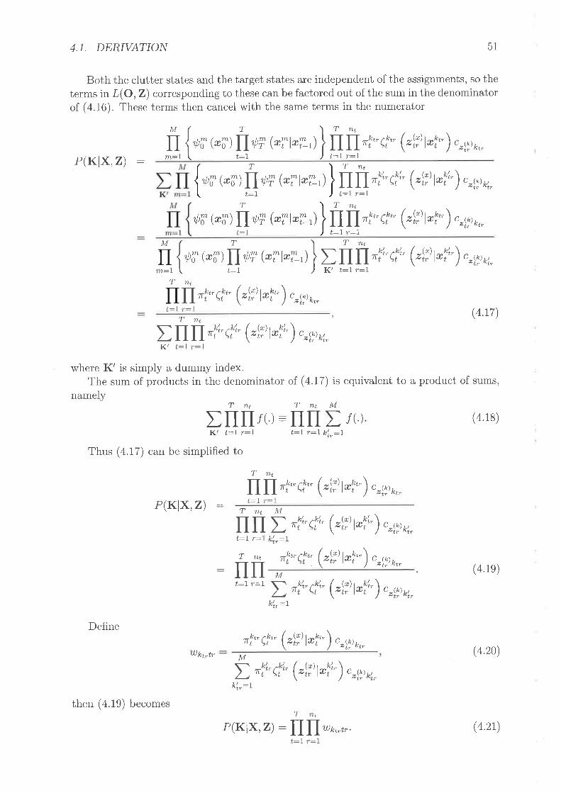
4.1. DERIUATION 51
Both the clutter states and the target states ar-e independent of the assignments, so theterms in tr(O, Z) corresponding to these can be factored out of the sum in the denominatorof (a.16). These terms then cancel with the same terms in the numerator
P(KI){-,Z) þ_{rr @i)II,þi @T *7,)}H nf*ef* ("Íi' *f-) ""Ít,r,.
,þi @i)Ilw (*Tl*7,)
T,þi @ÐlIvr @T@7,)
t:IT
t:I
il fi nli EkL. ("Íi, wf*),.Íy n;.t:l r:1
Milú fr nr,. cf- (,Íi, l*i*) ""Ír) *,.t:l r:7
{rr ønyr, (*?t*7) } p H ,rfL.çkí. ("Ír,wrr¡ ".Ít,r;.
il fr*f* e!" (,Íî,t,i") c"g)n,.
rn:lT
t:l r:l (4.t7)
(4.18)
(4.1e)
(4.20)
(4.2r)
Tntt il fnf; ç*|' ('Ír' wr") ""Ír) *i,Kt t:l r:I
where K/ is simply a dummy index.The sum of products in the denominator of (4.17) is equivalent to a product of sums,
namely
Thus (4.17) can be simplified to
P(KIX,Z)
Define
ú il nr" cf" (r',i'wr") "",,r.,n,"
TntTntMtilll/( )=lIlI t /( )Kt t-7 r:1, t:I r:l þt,:l
Tnt: I]IIt:l r:l
t:I r:lTntM
ilil D, "i;efr. (.Íî'l*lt.) ""g,)n,.f:l y:l þt,:!
nf ," <!,, ("1î' l*f ' ") " ",,1,
*,,
D "i;eit. (,1î,1*f,.) ""g,rL.
M
krr:t
nf,, ef, " (.Íî' l*f") " "'f;, r,,kt,tr M
\ nYt'çrt'k'tr:t
("Í;,1*i*¡ ""Ít)*,.
P(Klx, z):ilflrr,.,,Tnt
t:l r:l
then (4.19) becomes
'11)

52 CHAPTÐR 4. THE PMHT WITH CLASSIFICATION MEASUREMENTS
The w^¡, is referred to as the association weight for measurement r at scan ú andmodel m. It can be thought of as the posterior probability that the assignment k¿y : rnwhereas the prior probability is, by definition, ri. The weight u)^¿, is implicitly iterationdependent because it is a function of the estirnates at iteration ¿.
4.L.4 Expectation StepThe expectation step of the EM algorithm involves the calculation of the auxiliary func-tion, Q. Recall that the auxiliary function is defined in (4.9) as
8 (x,r, clx(¿), ¡(.,), ç(';)) : t log tr(o, z;fr,c)p (KlxØ,2.r@, C(r)¡ ,
K
where the dependence on the probability mass functions fI and C is shown explicitly. Thequantities ¡(';), ¡(l), and C(i) are the estimates found from the ¿¿h iteration of the EMalgorithm, and the estimates for the i + Lth iteration are found by maximising Q.
Fþom (4.15) write
rogtr(o, z;fr,C) : '"- {JI, {rr oy\r, (*Tt*7.)} x
Tnt
n I nf'" Çf* ("1î' l*f")' "tf' r,.\t:1. r:Irrr( T I: I { t"* ,þi @T) + t toeúi @Tl*7) I
----r I L:r )Tnt
+ t I {t"* r,n* + los #,' (rÍ;'Wf") r tog ",Í1.) t ,,} .f+.zzl
t:I r:7Substituting Ø.22) and (4.21) into (4.9) gives
I (X,fI, CIX(i), fl(i),6(t)) :
+ ^:D-{'"*r, @i) +å,"- 'þF
(*Tl'r')}
+ D {iË bs,rr''} ilii ,',t,),,,K ( r=L r:t ) t:1lJ
.Ð{åå ,,ec!" ("Í;'wr-) }Ug'*
.Ð{åå ros'"Ít'r"
Tnt
IIil'f).,,t:7 r:\
tr
'u)(ùkt,tr (4.23)
The notat ion wf,),r, is used to indicate that the measurement to model assignmentweight is calculated using the estimated states and parameters from iteration z, namely¡(t), ¡(;), and C(i).
The following two identities are used to sirnplify (4.23),Tnt
t il fl'wt*"t' : l' (4'24)K t:I r:I

4.1. DERIUATION
andTnt
t ilIJ,.r,,r,:utrusustK\/c'" f:l r:1
where t is the sum oveï all assignment indices except k?,s
K\k,"Applying (4.24) and (4.25) to (4.23) gives
I (x,fr, Clx(t), If(¿), c(e)¡
t t I to* '"',1;*'f),
rôo.)
Mtm:l
(r{ tosøä' @i) + Ito* ,þi @T *7IE
11.\wì*i.,
(4.25)
(4.26)
,)
.{
.{
.{
TntMttlto*t:I 'r:l k:lTnLMttI,o*
t:l r:l k:lTntM
nfw
ef (.1? *i)
t:I r:7 lc:7
(4,26) can be grouped into the following three terms
M
m:lg (x,fI, clx(i-1), ¡(r), c(t)) : Ðqç + t eh t es
T
t:l
The Qft term in (4.27) depends only on the target model states and the measutementsand is given by
TTnteT :toeúi @Ð + I to, ,þT @Tl*7,) + I I,o* ef ("Íî)@T) -f),,. (4.28)
t--I t:l r:7
(4.27)
(4.30)
The Q¿,, term in (4.27) depends only on the prior probability fI and is given by
Q,n:ttros"frf), (4.2e)r:l Ir:7
The Qs term in (4.27) depends only on the classification measurem"nt" ztf) and theconfusion matrix C and is given by
ntM
TntM
t:l r:1 k--IQc: ttlto* ""li,rrfll
4.L.5 Maximisation StepThe EM maximisation step updates the estimates of the unknown states and parametersby maximising the auxiliary function Q. Because the auxiliary function is the sum of

54 CHAPTER 4. THE PMHT WITH CLASSIFICATION MEASUREMENTS
independent tetms, the overall function can be maximised by performing independentmaximisation on each of the terms.
¡rn(i+l) : argmaxQft,T
If(¿+l): argmaxl.Qr,,t:1'
ç(l+t¡ : arg rnax Q6.
4.L.5.L State estimate
The maximisation of the state terms Çp depends on the particular forms of the evolu-tion probabilities ,þT@Tlæ7,) and the measurement processes efQÍ?læi) anð, may bedifferent for each model since the models may have functionally different probabilisticmodels. For the special case of linear Gaussian functions, Streit and Luginbuhl haveshown that the solution for the states is a fixed interval Kalman smoother. The proof ofthis important result is repeated for completeness.
Let us examine the measurement term in (4.28) which is given byTntt trogcr (,Í?wr) -fl,,
t:l r:IFor the case of linear Gaussian statistics, the measurement function for model m is
er (,lr)@T) : "#p""0
{ -}(,Sl - HT,T)'(*r)-' ('Í:' - Hr*T)} ,
where Hi" is an appropriately sized matrix and R is the measurement covariancedetail on linear Gaussian models is given in section 3.3.
Taking the log of (4.31) gives
(4.31)
More
Tnt
D'l),,'Íi)r:I
(Rr)-'uT*T)
- FT *T)' (nî")-' (ä,r..fr') ) + A (4 34)
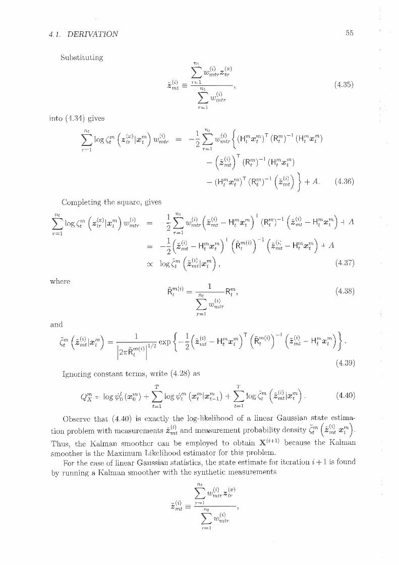
4.1, DERIUATION
Substituting
into (4.34) gives
nt
where
I tosç" ('Íî'@r),9,,
D'f),,'Íi'r:l
(r)wrnt,
1
Ð'l),,r:7
Ri"
(¿)tnta
55
(4.35)
(4.36)
(4.38)
nttr:1
r:1
Completing the square, gives
;2.n {FT*T). (Rr)-' (ur*T)
- (rn)'(*r)-' UT*T)
- FT*T)'(nr)-' ?Ð) * o
É.* er (,1î)@T),9,.r:l
: -;i.9,,(zl), - HT*T)'(*r)-' ?n - aiæi) + ar:7
: -i|n - HT*T) (n¡t'r¡ ' (t9, - niæi) + 'a,
o( bsef (u9,1-f) , Ø.37)
ñirtr
and
r: (29,1*7) ' (rg, - HT-T)\1
{-;('r - HT*r) (nr"')r/2 exp2rAYU't
(4.3e)
Ignoring constant terms, write (4.23) as
TTQT:ros,þL@i) +Ito* ,þT @Tl*r:.') * I roeef (u9,1-f) (4'40)
t:L t:l
Observe that (4.40) is exactly the log-likelihood of a linear Gaussian state estima-
tion problem with measurem e*s 2flrand. measurement probability density ç (r|tl-f)Thus, the Kalman smoother can be employed to obtain X(i+1) because the Kalmansmoother is the Maximum Likelihood estimator for this problem.
For the case of linear Gaussian statistics, the state estimate for iterationi,lT is foundby running a Kalman smoother with the synthetic measurements
nt
Ð'(;Ì,,'li)r:7
D'f),.r:I
- (i\þn¿t:
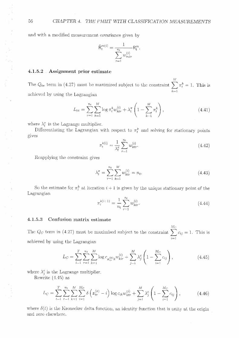
56 CHAPTER 4. THE PMHT WITH CLASSIFICATION MEASUREMENTS
and with a modified measurement covariance given by
ñ¡r,'l
D'l),.r:7
Rr
4.L.5.2 Assignment prior estimatefuI
The Q¡n term in (4.27) must be maximised subject to the constraint D"! : t This is
1
where Àfl is the Lagrange multiplier.Differentiating the Lagrangian with respect Lo r! and solving for stationâry points
gives
(4.42)
Reapplying the constraint gives
achieved by using the Lagrangian
achieved by using the Lagrangian
Ltu : äär* r! wf)+ .u (r - P_",)
. flt
nfþ) : t \-L \lt lr/trL --1
lxluií,
^;
Mtj:t
k:t
i:r
(4.41)
)i: ntMtt'fl,:n,r:I k:I
(4.43)
(4.44)
(4.45)
So the estimate for rf at iteration ¿ -|- 1 is given by the unique stationary point of theLagrangian
k(i+r\ttt
nt
D,'ÍlIr:7
4.L.5.3 Confusion matrix estimateM¿
TheQs term in (4.27) must be maximised subject to the constraint D"o,:1. This is
TTÙ¿
M¡1
Lc: tIDto* c"ytrwf;),+ 1-tTntM
t:l r:I k:I i,:7
where Àrq is the Lagrange multiplier.Rewrite (4.45) as
C;;
i:L
MçTntMMcMLc :t t t t õ ('Íf) - ,;) ros
"on-f),+ I r; 1-t C;; (4.46)t:I r:I lr:7 i:I j:r
where ô(ú) is the Kronecker delta function, an identity function that is unity at the originand zero elsewhere

4.2. SUMMARY OF THE PMHT-C ALGORTTHM
t:7 r:l i:Int nt
Differentiating the Lagrangian with respecl, to c¡¡ and solving for stationary pointsgives
"11) :: É 'Lu (;,i' - r),j',), (4 47)_xJ
Àr¡ i:, ,:,Reapplying the constraint gives
n¿ rLt M¿
^; : ItD6('ti) -u),5',1
57
II,jl) Ø48)Ã ':t
So the estimate for c¿¡ at iteration ¿ i 1 is given by the unique stationary point of theLagrangian T n¿tt 6 ('Íi) -n)'l',1
(i+1)-1,1
t:7 r:7 (4.4e)nt nt
D,L,'l:)"t:l r:l
The denorninator of (a.a9) is the sum of all the weights for model j over the wholebatch. This is the posterior maximum likelihood estimate of the number of measurementstruly caused by model j. The delta function in the numerator effectively controls the rangeof the summation in the numerator by selecting only those weights which correspondedto classification measurements with value i. So, the numerator is the posterior MLE ofthe number of measurements truly caused by model 7 with classification i. The ratio in(4.,19) is thus an estimate of the fraction of measurements due to model j which gave riseto an observed classification ¿. In other wotds, the estimator for each confusion matrixentry (which is a probability) is the estimated relative frequency of the associated event.This is an intuitively appealing result.
4.2 Summary of the PMHT-c algorithmThe Probabilistic Multi-Hypothesis Tracker with classification measurements (PMHT-c)can be summarised by the following steps.
1. Initialise the state and parameter estimates, X(o), lI(0) and C(0) . Proper initialisationis crucial since the EM algorithm is a hill climbing approach that can guarantee onlylocal convergence. Since the classification measurements, zlf are observations ofthe assignments, it is possible to use their probabilities to define .çri) : c,txt*ãrrdform the initial estimates using these weights.
2. Calculate assignment weights w::)tu for each measurement r and model rn at eachtime sample ú defined by (4.20) as
(i) - nf@ ef ('lî'l*T''') ""rr,^
rntr - M
Ð".'ùel (.Ír'tI:I
(h)tr
*'r''') "
'u)

58 CHAPTER 4. THE PMHT WITH CLASSIFICATION MEASUREMENTS
3. Calculate the refined estimate of the states X(i+l) using the weight s w:ltu and theobservatiotrs z¿y.
For the case of linear Gaussian statistics, the state estimate for iteration ¿ * 1 isfound by running a Kalman smoother with the synthetic measurements
nt
D'[1,,'Íi'='(i) -
r:l-mt - T¿I )
Ð'f)"r:l
and with a modified measurement covariance given by
nTro¡ - -!-orD'f)"r:1
where Ri is the true measurement covariance, i.e. the covariance of the functionlrnIr
4. Calculate the refined estimate of the assignment prior, II(i+l), using.nt
irk(i+t) : )>,r,;),tbtf': I
5. Refine the estimate of the confusion matrix, C(i+1) using
T nt
ID¿ ("Ír' - u),!:,1
"\i+- x.l
1) _ ¿:1 r:1nt nt
DD,l:),t:7 r:7
6. Calculate the value of the auxiliary function at the new estimates,
I (Xtr+tl,If(¿+l), C(i+l)lX(i), ¡(r), C(i)) :Mt roe,þi ('pto*'r¡ + t .s,þi (æ7{t+'t'',T}i*'))
T
t:1m:l
.{
.{
.{
TntM
ItDto*nfo+rtru)t:l r:7 k:7TntM
t:l r:l le:lTntM
IDItosef ("Íî'l*f''*") (i)'11) ktr
ÐÐÐ'"* "')¡i¡'Y¡'
6 until I (Xf;+t¡,fI(,+t), C(i+1) ¡(r), ¡(r), C(¿)) converges7, Repeat steps 2

4,3, SPECIAL CASES 59
4.3 Special Cases
Consider two special cases of the PMHT-c filter. In both cases, it is assumed that thePMIIT knows the true confusion matrix C.
4.3.t Uninformative classification measurements
The PMHT-c is a generalised version of the original PMHT. The original PMHT is derivedwithout classification measurernents, so it is expected that the PMHT-c will simplify tothe original PMHT in the case that the classification measurements are uninformative.
Suppose that the classification nìeasurements were uninformative, that is each modelis equaliy likely to give rise to each class output. In this case, the confusion matrixis constant across rows. That is, c¿j c¿¡rYi,,j,k. Denote c¿ as the constant value ofthe confusion matrix for row ¿. This situation is equivalent to having no classificationmeasurements at all since the probability of the observatio " tlf) is independent of thevalue of k¿r, ,.".
" "Íf, rr, : c
"Í!) .
In this case, the weight equation for model rn becomes
,,f@ ef (.Íî'l*T'u C tt¡'t(i)Um'tr M
Ð"',Ø el ("Íî'l*i''') (r. )trL- L
Ctx'tr ,ni(o) eT ("Íî'l*Tt")
M
" "Íi, D rl{a r' (,Íî' l*i''')l:7
,,f@ ef (,Íî'l*T'''M
Ð"',(ùel (,Íî'l*i''')t:7
The term due to the classiflcation measurements cancels and the weight equation isthe same as that for the standard PMHT. Thus, when the classification measurementsare uninformative, the algorithm simplifies to the standard PMHT.
4.3.2 Perfect classification measurements
Another special case of interest is when the output of the classifier is perfect. Supposethere is a separate class for each model and that the classification measurements ate errotfree. In this case, the confusion matrix is the identity matrix and the individual elementsmay be written as identity functions c¿¡ : õ(i, - j). Intuitively, it is expected that thealgorithm should use the classiflcations as hard associations.
c

60 CHAPTER 4. THE PMHT WITH CLASSIFICATION MEASUREA4E¡\ITS
-t0
40 60 80 -1 20 40 60 80time sample time sample
(a) crossing targets (b) turning targets
Figure 4.1: Simulated scenarios
In this case, the weights become
c.o.=qoo
C
Eoo-
-1
-1
r!*Q)çn,. (rlî,@f",,t) d (rÍi) - r,,)tr)tu ¡rr,t, M
Ð"',(ù e' ("Íî,1*i,',) d ("li) - t)l,--7
-ltt,ttt(i) ¡kt,
Sr zlllæf*{t) "lP - k*6
fß),., tk)*zir'\L) tzirttt \¿ zll)piÍi)ra
:u(*r,-.Í?)This weight equation effectively means that the filter no longer uses probabilistic as-
signment of the observations and models. This should be expected since the perfect clas-sification measurements are providing the filter with the true values of K. The weightsare now hard assignments independent of the model states so there is no need for re-cursive estimation of the states or the probability parameter fL The filter simplifies toindependent state estimation of the different models using the assignments provided bythe classifier.
4.4 Performance AnalysisThe improvement in tracking performance obtainable by using classification measurementsis now illustrated through some simulated examples. These examples focus on estimationperformance in a manoeuvring target setting. Two different scenarios are considered.In each scenario, there are two targets that follow one dimensional trajectories that areclosely spaced, making for a difficult tracking problem. In the first scenario, the targetsmove together and then cross over before eventually diverging. In the second scenario, thetargets move together and then turn back. These two scenarios are shown in figure 4.1.The trajectory of target 1 is shown as a solid line and the trajectory of target 2 is shownas a dashed line.
In both cases, the targets are simulated without clutter and a single measurement isobserved in each scan. The measurement is taken from either target with equal probability.

4.4. PERFORMA¡\ICE A¡üALYSIS 61
The sensor receives measurernents of position and classification measutements. Theclassification measurements are an observation of the true source of the position observa-tion. The confusion matrix for the classification measurements is of the form
C-
where a is the probability that the correct classification is reported. a will be referred toas the classification veracity. The scenarios are tested with various values of a and theperformance observed. For the case of a:1, the classification measurements are perfectand the filter performance will be the best possible for the scenario. Thus, the case of a : 1
provides a performance bound. For the case of a : 0.5, the classification measurementsprovide no information and the PMHT-c simplifies to the standard PMHT. Thus, theperformance when a : 0.5 shows the standard PMHT performance on the scenario. Thecases of known and unknown C were both considered.
4.4.L Simulation DetailsThe particulars of the simulations used for performance evaluation are now presented.For each combination of parameters, 1000 Monte Carlo realisations are generated and thefilter performance is gauged by averaging over these realisations.
4.4.L.L Target Trajectories
In both scenarios, the target trajectories are composed of constant velocity and constantacceleration segments. This means that the position is a piecewise combination of linearand quadratic functions. The trajectory of target 2 is a mirror image of the target 1
trajectory. The difference between the turn scenario and the crossing scenario is the signof the acceleration in the second constant acceleration segment.
For the crossing scenario, the true state of target 1 is given by:
al-a
7-aa
(4 50)
(4.51)
rå+
i+
rl"
-u
-u
-u i ft(r - z0)0
-hî - 50)
0<-r <2020<r<30
r<50r<60
0<r <20
r<80
30<50<60<
20<r<3030<r<5050<r<6060<r<80
r[-urr[-zou-h?-20)'r[ - zsur[-zsu-hî-bo)'r[-aoo-u(t-60)
r d¿
(4.52)
where the constants u : 0.5 and rå : 1 '125u: 13.5 were chosen. The function given in(4,52) defines the solid curve shown in figure a.1(a).
4.4.L.2 Measurements
At each scan' a single measurement is observed, TLt: I' The scans are taken at regularintervals with a sampling rate of 1. This means Lhal, r¡: ú and Tt - rt_t: 1. A batch

62 CHAPTER 4. THE PMHT WITH CLASSIFICATION MEASUREMENTS
length of T :80 is used. The measurement at each scan is taken from either target withequal probability, so rl : 0.5. lI is assumed to be known by the tracker.
Each measurement is the current position of one of the targets corrupted with whiteGaussian noise, with variance R : 1.
The classification measurement at each scan is generated according to the confusionmatrix, C, as defined in (4.50). The classification veracity, o, is varied.
4.4.L.3 Target Models
The tracker uses a one dirnensional almost constant velocity modell for the targets. Thismeans that the motion is assumed to be constant in velocity with Gaussian perturbations.In the one dimensional case, these perturbations are scalars with zero mean and variancea This variance is assumed to be constant and the same for both targets. A value ofq : (u/10)2 : 0.0025 was chosen so that the filter would give an adequate dynamicresponse to the acceleration segments. The target state vector is
rir\T
The true measurement process is linear and Gaussian. It is assumed that the filterknows the measurement process. This measurement process is, in the Gaussian positiononly case, described in 3.3. So, the measurement probability density used by the filter is
ri (4.53)
Ìm\ (") *r) {-* (":o -H*T)'}, (4.54)
where R:1is a scalar, and 11 : [1,0].The filter knows that the confusion matrix, C, takes the form given in (a.50). Both
cases of known and unknown classification veracity) e.) ate considered. When the valueof o is unknown, the confusion matrix must be estimated. However, the filter does knowthe form of the matrix, which can be exploited by incorporating the constraint c11 : c22.When this constraint is incorporated into the iterative maximisation of Qc, then theestimator for a is given by
T
Ð.\',, d ("t^ - r) +.1')a (zt:l
The target state estimates for the filter are initialised by using the correct initial stateand projecting a constant velocity path from this point. This scheme is unrealistic inpractice, but it avoids irrelevant track initiation issues. Track initiation is consideredlater in chapter 6. The prior state distribution tþ*(r|) is Gaussian centred on the correctinitial state with covariance matrix Po : diag(,R,0.5).
4.4.2 Performance MetricsThe performance of the PMHT-c is quantified by estimation accuracy for X and C as a isvaried. An additional measure of performance is the probability that the filter follows thetarget trajectories properly. Since the measurements make the target paths ambiguous,it is possible that the filter may lose the targets, or may switch tracks. Figure 4.2 showsexamples of trials with correct and incorrect tracking. In the left plot, the filter hascorrectly identified the crossing trajectories, but in the right plot, it assigns measurementsfrom target 2 to the track for target 1 and so incorrectly produces turning trajectories.
6(z+1) : ! [7l (À) (4.55)2
lrefer to section 13.3 for more detaiÌs on the almost constant velocitv mo<ìel

4.4. PER.FORMAATCE A¡úALYSIS
-10
'15
10
5
40time sample
63
60 80
c.EØoo-
Ã
-Ã
coØoo
-1
-1 -120 40 60 80time sample
(a) crossing trial, correct tracking
Figure 4.2:
(b) crossing trial, incorrect tracking
Examples of simulated trials
20
The probability of correctly following the trajectories is estimated by counting thenumber of random trials where both of the state estimates remain within a prescribeddistance of the respective true states, If the tracks move farther away from the true statethan this distance at any stage, then the trial is declared incorrectly tracked. A gate
distance of 3 units was used.The estimation performance for X is quantified by the bias and variance of the esti-
mator output. These statistics are calculated using their sample estimates for trials withcorrect tracking. The estimation of target 1 is investigated and it is assumed that similarresults would be obtained for targeí 2 (particularly given the symmetrical nature of thegeometry). Spot checks confirm this assumption.
The instantaneous position bias is estimated from the simulations by using the samplemean of the estimates. That is,
Êî: lNË fn:Itl(") _ rl), (4.56)
where fr1("1 'r the position estimate for track 1 at scan ú from the nth correctly trackedrandom trial. l/ is the total number of trials with correct tracking.
There are two sources of estimation bias. Firstly, the model used by the PMHT-cdoes not properly match the target dynamics. The true target model switches betweenconstant velocity to constant acceleration during the scenario. The tracker is attemptingto model the trajectory using an almost constant velocity model, which means it will beinclined to estimate a trajectory with gradual changes in speed. During the periods ofacceleration, the model is mismatched and the tracker models the manoeuvre as a moregradual acceleration over a longer time period. This leads to estimator bias. The secondsource of bias is the presence of measurements from the other target. The measurementstruly due to target 2 will be given a non-zeÍo assignment weight for target 1, and willcause a bias towards target 2. This bias depends on the target geometry because theassociation probability will be very low when the targets are widely separated. If thetracker were able to perfectly assign measurements, then the second target would cause
no bias. These two sources of bias will be referred to as mismatch bias and assignmentbias. The biases rnay counteract each other. For example, in the turn scenario, themismatch bias on target 1 is positive (the expected value of the estimate is above the true

64 CHAPTER 4. THE PMHT WITH CLASSIFICATION MEASUREMENTS
trajectory) but the assignment bias is negative. In such a case, the mismatch bias maybecome masked if the assignment bias is high (when the classifier veracity is low). Thebiases are not inherent deficiencies of the PMHT approach, but inevitable errors that anyestimator would encounter using the above target models.
The instantaneous position variance is estimated from the simulations by using thesample variance. That is,
1¡/òT : :I lr;,"' - (er* "i)] Ø57)-L N 1,
Estimator variance is caused by the randomness of the measurements. \Mhen the variabil-ity of the measurements assigned to a track is high, then the estimator variance is high.Such a condition is encountered when the two targets are close together. If the trackerperformed perfect assignment (such as when the classifier veracity is unity), then the mea-surement variability would always be the target measurement noise, and the estimatorvariance wouid be constant with time.
The estimation of the confusion matrix is quantified by examining the bias and varianceof the estimator â obtained when the PMHT-c converges. These are estimated using theirsample values, namely
¡lBa: 1
N I lat"r - o) ,
n:1(4.58)
(4.61)
ão : :Ë laøt - (er *")]' (4be)N t:t
The bias and variance of the estimator ã. are not time varying because ô produces oneestimate for the whole batch.
For each scenario, the number of trials with correct tracking is an estimate of the trueprobability that the scenario is correctly tracked for a particular value of a. Let us denotethe true probability of correctly tracking the scenario as p. The estimator, þ, used to formthe tables of results is
1åþ: ñ )-,d0, (4'60)i:I
where d¿ is the result of the ith ftiaI (zero or unity) and lr/ is the number of trials, i.e 1000.It can be shown that the variance of this estimator is given by
var(p) :*(o-p').
This is maximized when P:0.5. If p:0.5 then the variance of þ using 1000 samplesis 2.5 x 10⁻⁴. Thus, the standard deviation of the results given in tables 4.1 . ..4.4 is lessthan 0.016, i.e. 16 trials.
4.4.3 Improvement with known confusion matrixFirst investigate the performance gain obtained by using classification measurements whenthe confusion matrix C is known. The number of trials with correct tracking for variousvalues of a is given in table 4.1.

4.4. PERFORMA¡\rCE A¡úALYSIS
0.5 0.6classification veracity, a
0.7 0.8 0.9
863 972 1000
65
1
crossing targets
turning targets
634 613 694
115 355 695 911 987 1000
Table 4.1: Nurnber of trials with correct tracking with known confusion matrix
As would be expected, the number of triais with correct tracking generally increasesas the classification veracity improves. What is surprising is how much improvement isobtained even for very inaccurate classifications.
The standard PMHT (namely the PMHT-c with a : 0.5) performs poorly on the turnscenario because the fllter is predisposed to the crossing explanation. The filter tends toovershoot, causing the tracks to cross in the stationary part of the scenario. Since thetracks have already crossed, it is unlikely that they will cross again, which is required forthe turn output. This behaviour can be seen from the estimator bias at the middle ofthe scenario (refer to figure 4.5). The bias that causes the overshoot is the assignmentbias, which reduces as the classification veracity improves. The assignment bias actuallyimproves the performance for the crossing scenario. Table 4.1 shows that the performanceof the PMHT-c is better for a : 0.5 than for a : 0.6 on the crossing scenario. This isbecause the assignment bias for the filter predisposes the filter to the crossing case.
The position estimation bias for the crossing scenario is plotted in figure 4.3 for variousvalues of a. The variance for the crossing scenario is plotted in figure 4.4. Figures 4.5and 4.6 show the bias and variance for the turning scenario respectively.
The algorithm uses smoothing which means that measurements from earlier time sam-ples and measurements from later time samples contribute to the state estimate. Becausethe smoother does not have these extra measurements near the end of the batch, the vari-ance rises towards the end. At the beginning of the batch, the variance is very low. Thisis due to the initialisation which uses the true value of the target state. This behaviouris common for all classification veracity values, o. When ù.: l, the true source of eachmeasurement is known, and the variance is roughly constant over the rest of the batch.There is a small rise in variance during the target manoeuvres, wltete the assumed modeldoes not fit the true dynamics, and other fluctuations are due to the finite ensemble size.
For other values of a, the variance peaks around the middle of each scenario. This iswhen the two targets are close together, and there is most ambiguity in the assignment ofmeasurements. The height of this peak increases as o decreases. In the turning scenatio,the peak of the variance is roughly symmetrical in time, but it is not in the crossingscenario. This is because the target trajectories are symmetrical in the turning scenario,but not in the crossing one.
As discussed in section 4.4.2, there are two sources of estimator bias, namely the mis-match of the target dynamics and the assumed model dynamics during target manoeuvres)and incorrectly associated measurements from the other target. The first source is mostclearly seen in the curves for perfect classificatiolt, û:1. In this case, there is no associ-ation errors, and the only source of bias is the model mismatch. The algorithm assumesan almost constant velocity model, but the true trajectory follows a constant accelerationIaw during the manoeuvres. This means that the algorithm over-smoothes the estimatedtrajectory, rounding off the corners and introducing bias towards the inside of the turn.For the crossing scenario, this means a positive bias for the first manoeuvre, and a neg-

66 CHAPTER 4. THE PMHT WITH CLASSIFICATION MEASUREMENTS
05
0
at,.g-oorúEao
-05
-1
-1 .5
10 20 30 40t¡me step
50 60 70 80
Figure 4.3: Bias of estimator î|, C known, crossing scenario
0 10 20 30 40time step
50 60 70 80
o()c.a(ú
o(úEU)(l)
0.9
0.8
0.7
0.6
0.5
0.4
0.3
0.2
0.1
0
0=1o=0.9c=0.8a=O.7cr=O.6o=0.5
- o=1
- - cx=0.9o=0.8.- a-0.7
- - o=0.6ü=0.5
Figure 4.4: Yariance of estimator î1, C known, crossing scenario

4.4. PERFORMA¡\rCE A¡üALYSß
0.5
67
0
-05U).q_o
o(úEØ0) -1
-1 .5
-2 40 50 60 70 800 10 20 30time step
Figure 4.5: Bias of estimator î1, C known, turning scenario
0.3
0.2
0.1
00 10 20 30 40
time step50 60 70 80
1
oo.q(ú
o(úEoo
0.9
0.8
o.7
b
05
0
40
cx=1
ct=O.9u=0.8a=0.7a=0.6a=0.5
o=1u=0.9tx=O.8s=0.7o,=0.6s=0.5
Figure 4.6: Variance of estimator f|, C known, turning scenario
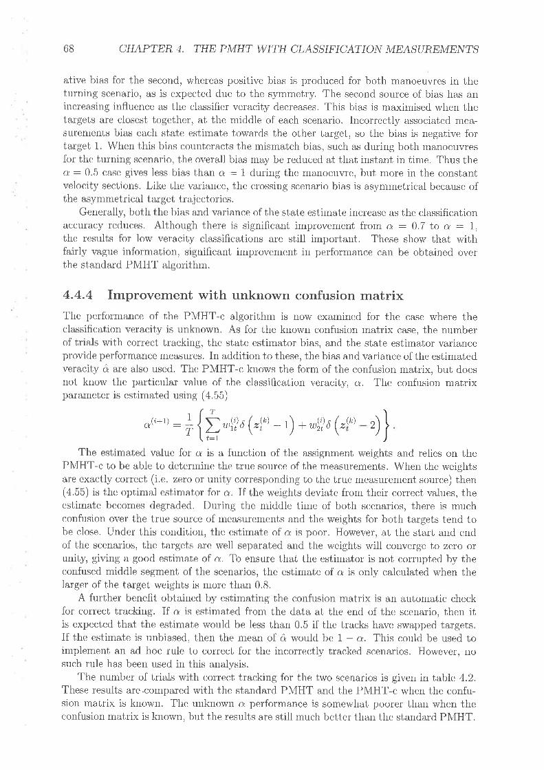
68 CHAPTER 4. THE PMHT WITH CLASSIFICATION MEASUREMENTS
ative bias for the second, whereas positive bias is produced for both manoeuvres in theturning scenario, as is expected due to the symmetry. The second source of bias has anincreasing influence as the classifier veracity decreases. This bias is maximised when thetargets are closest together, at the middle of each scenario. Incorrectly associated mea-surements bias each state estimate towards the other target, so the bias is negative fortarget 1. When this bias counteracts the mismatch bias, such as during both manoeuvresfor the turning scenario, the overall bias may be reduced at that instant in time. Thus thea : 0.5 case gives less bias than a : 1 during the manoeuvre, but more in the constantvelocity sections. Like the variance, the crossing scenario bias is asymmetrical because ofthe asymmetrical target trajectories.
Generally, both the bias and variance of the state estimate increase as the classificationaccuracy reduces. Although there is significant improvement from o : 0.7 to a : 1,the results for low veracity classifications are still important. These show that withfairly vague information, significant improvement in performance can be obtained overthe standard PMHT algorithm.
4.4.4 Improvement with unknown confusion matrixThe performance of the PMHT-c algorithm is now examined for the case where theclassification veracity is unknown. As for the known confusion matrix case, the numberof trials with correct tracking, the state estimator bias, and the state estimator varianceprovide performance measures. In addition to these, the bias and variance of the estimatedveracity ô are also used. The PMHT-c knows the form of the confusion matrix, but doesnot know the particular value of the classification veracitv, a. The confusion matrixparameter is estimated using (4.55)
Tû(i+1) : + {t ,\')a (,f) - t) * ,y)6 (a
(k)2
t:7The estimated value for a is a function of the assignment weights and relies on the
PMHT-c to be able to deterrnine the true source of the measurements. When the weightsare exactly correct (i.e. zero or unity corresponding to the true measurement source) then(4.55) is the optimal estimator for o. If the weights deviate from their correct values, theestimate becomes degraded. During the middle time of both scenarios, there is muchconfusion over the true source of m.easurements and the weights for both targets tend tobe close. Under this condition, the estimate of o is poor. However, at the start and endof the scenarios, the targets are well separated and the weights will converge to zero orunity, giving a good estimate of a. To ensure that the estimator is not corrupted by theconfused middle segment of the scenarios, the estimate of a is only calculated when theIarger of the target weights is more than 0.8.
A further benefit obtained by estimating the confusion matrix is an automatic checkfor correct tracking. If o is estimated from the data at the end of the scenario, then itis expected that the estimate would be less than 0.5 if the tracks have swapped targets.If the estimate is unbiased, then the mean of ô would be 1 - o. This could be used toimplement an ad hoc rule to correct for the incorrectly tracked scenarios. However, nosuch rule has been used in this analysis.
The number of trials with correct tracking for the two scenarios is given in table 4.2,These results are -compared with the standard PMHT and the PMHT-c when the confu-sion matrix is known. The unknown a performance is somewhat poorer than when theconfusion matrix is known, but the results are still much better than the standard PMHT.
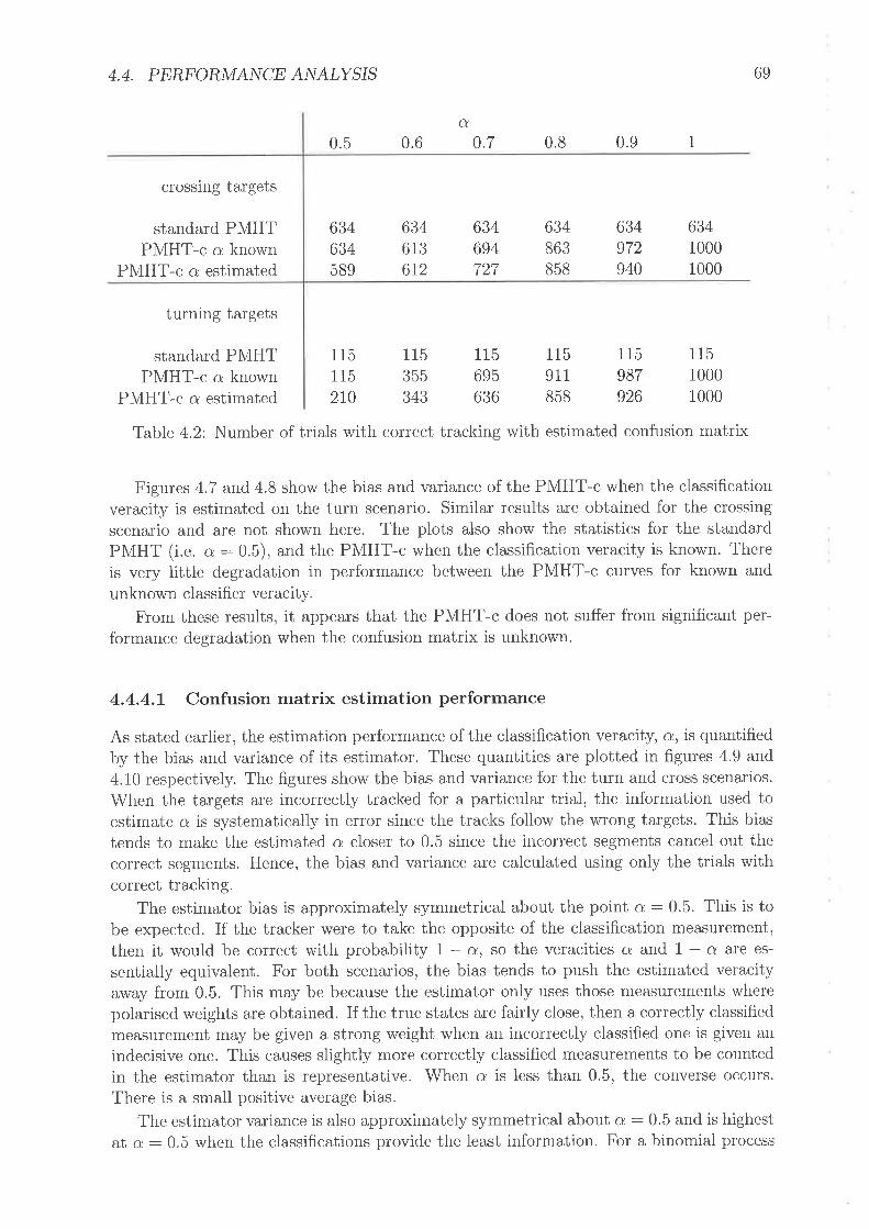
4. 4. PERFORMA¡\|CE A¡\IA¿YSIS
0.5
crossing targets
standard PMHTPMHT-c a knowrt
PMHT-c a estimated
turning targets
standard PMHTPMHT-c o knowrr
PMHT-c a estimated
69
a0.6 0.7 0.8 0.9 1
634634589
634613612
634694727
634863858
634972940
63410001000
11510001000
1151152r0
115911858
115987926
115695636
115355343
Table 4.2: Number of trials with correct tracking with estimated coufusion matrix
Figures 4.7 and 4.8 show the bias and variance of the PN4HT-c when the classificationveracity is estimated on the turn scenario. Similar results are obtained for the crossingscenario and are not shown here. The plots also show the statistics for the standardPMHT (i.e. a : 0.5), and the PMHT-c when the classification veracity is known. Thereis very little degradation in performance between the PMHT-c curves for known andunknown classifier veracity.
Flom these results, it appears that the PMHT-c does not suffer from significant per-formance degradation when the confusion matrix is unknown.
4.4.4.L Confusion matrix estimation performance
As stated earlier, the estimation performance of the classification veracity, o, is quantifiedby the bias and variance of its estimator. These quantities are plotted in figures 4.9 and4.10 respectively. The figures show the bias and variance for the turn and cross scenarios.When the targets are incorrectly tracked for a particular trial, the information used toestimate a is systematically in error since the tracks follow the wrong targets. This biastends to make the estimated o closer to 0.5 since the incorrect segments cancel out thecorrect segments. Hence, the bias and variance are calculated using only the trials withcorrect tracking.
The estimator bias is approximately symmetrical about the point a : 0.5. This is tobe expected. If the tracker were to take the opposite of the classification measurement,then it would be correct with probability I - a, so the veracities a and I - a are es-
sentially equivalent. For both scenarios, the bias tends to push the estimated veracityaway from 0.5. This may be because the estimator only uses those measurements wherepolarised weights are obtained. If the true states are fairly close, then a correctly classifiedmeasurement may be given a strong weight when an incorrectly classified one is given anindecisive one. This causes slightly more correctly classified measurements to be countedin the estimator than is representative. When o is less than 0.5, the converse occurs.There is a small positive average bias.
The estimator variance is also approximately symmetrical about a : 0.5 and is highestaL u :0.5 when the classifications provide the least information. For a binomial process

70 CHAPTER 4. THE PMHT WITH CLASSIFICATION MEASUREMENTS
cx =0.5 ü =0.60.5
020
0.5
-1.5
-2
00(t)(úõ -o.so(úE1U)o
-1.5
-2
U)(úã -o.sLo(úE1U)o)
0.5
40time step
u=O.7
40time step
o =0.9
40time step
60 80
60 80
60 80
020 40time step
s =0.8
40time step
c¿ =1
40time step
60 80
60 80
0.5
-1.5
0
5-0.U)(üão(úEu)(¡)
0
-0.5Ø
.(ú-oLo(gE(t)c)
1
-2
00
-1.5
0.5
-2020
020
0.5
020
020
U)(úõ -o.so(úE{u)o)
-1.5
-2
U'(úã -o.sLo(úcL1
U)o
-1.5unknown
- - 0 knownPMHT
-2
Figure 4.7: bias of estimator fl, C estimated, turning scenario
60 80

4.4. PER.FORMA¡úCE A¡úA¿YSIS
cr =0.5
020 40time step
a=0.7
0.8
60 80
60 80
20
020
cx =0.6
40time step
cx =0.8
40time step
Cr =1
7I
60 80
60 80
60 80
0. 8
0.6
0
0
oo(ú
(ú
Lo(úEao
ooc(ú'Ë 0.6
oq 0.4E.F(t)o
0.2
.4
.2
000
1
0.8 0.8
0.6
.80
0.6
.40
o.2
ooc(ú'=(ú
Lo(úEU)o
0.6
0.4
.2
0
0
ooc(ú
(ú
Lo(gEU)o
00 20 40
time step
cr =0.9
40time step
1
0.8
.40
o.2
q)oc(ú'=(ú
Lo(úE(t)(¡)
q)()c(ú'Ë 0.6Log 0.4Þ.FØo
0.2
0 0020 60 80 020 40time step
/
unknowns knownPMHT
Figure 4.8: variance of estimator fl, C estimated, turning scenario

72 CHAPTER 4, THE PMHT WITH CLASSIFICATION MEASUREMENTS
0.05
0.04
0.03
0.02
-0.01
-0.02
-0.03
-0.04 0.4 0.5 0.6classifier veracity, 0,
Figure 4.9: Bias of the estimator, ô
a.g-oo(úEU'o
001
0
(¡)o(ú
(d
o(U
EØo
0.01
0.009
0.008
0.007
0.006
0.005
0.004
0.003
0.002
0.001
0 0.1 0.2 0.3
0.1 0.2 0.3
0.7 0.8 0.9 1
o.7 0.8 0.9 10.4 0.5 0.6classifier veracity, d
- crossrng scenano
- - turn scenario
- crosstng scenano
- - turn scenariofitted curve
Figure 4.10: Variance of the estimator, ô
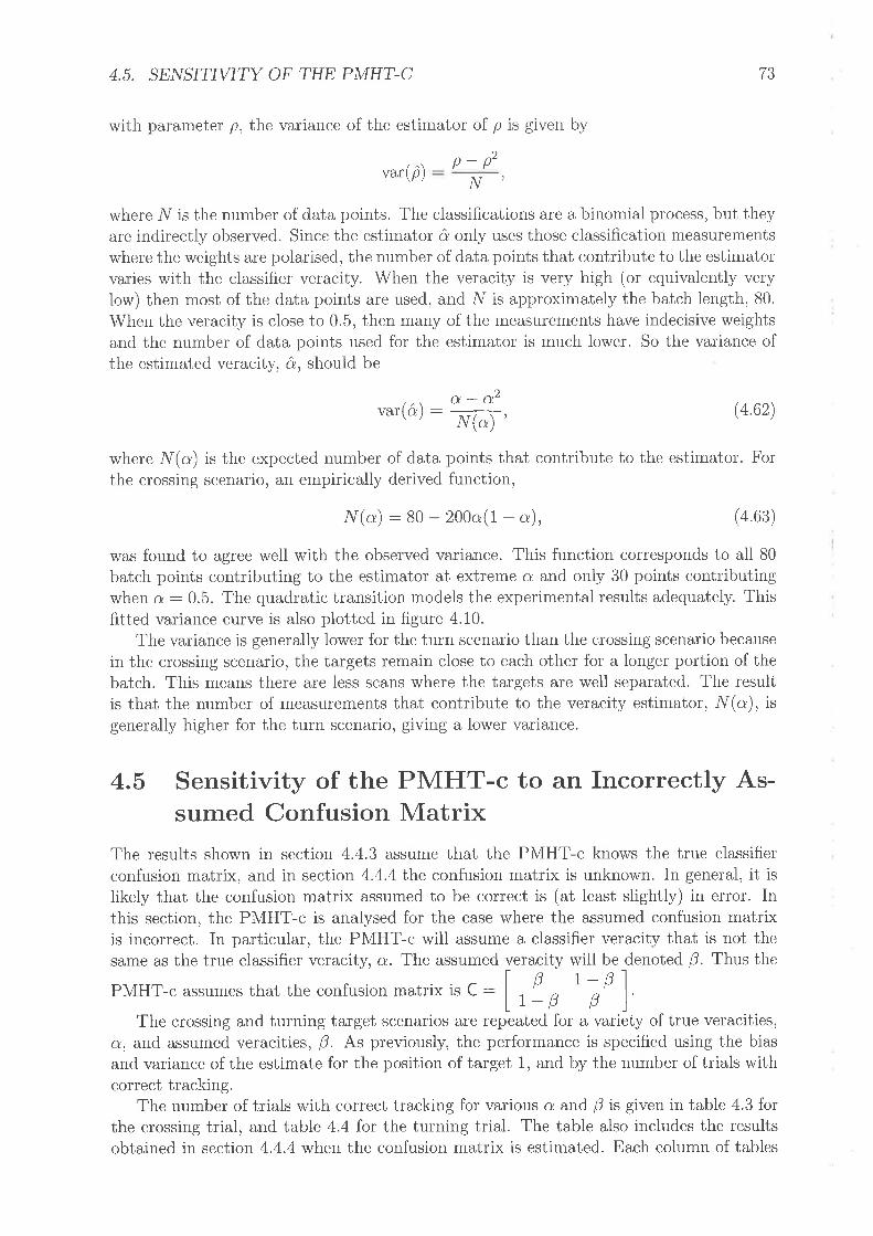
4,5. SENSITIYITY OF THE PMHT-C t.f
with pararneter p, the variance of the estimator of p is given by
var(P) o;" ,
where l/ is the number of data points. The classificatious are a binomial process, but theyare indirectly observed. Since the estimator ô only uses those classificatiolì measurementswhere the weights are polarised, the number of data points that contribute to the estimatorvaries with the classifier veracity. When the veracity is very high (or equivalently verylow) then most of the data points are used, and N is approximately the batch length, 80.
When the veracity is close to 0.5, then many of the measurements have indecisive weightsand the number of data points used for the estimator is much lower. So the variance ofthe estimated veracity, ô, should be
var(ô) : T#, Ø.62)
where ¡/(r) is the expected number of data points that contribute to the estimator. Forthe crossing scenario, an empirically derived function,
¡/(r) : 80 - 200a(1 - o), (4.63)
was found to agree well with the observed variance. This function corresponds to all 80
batch points contributing to the estimator at extreme a and only 30 points contributingwhen a : 0.5. The quadratic transition models the experimental results adequately. Thisfitted variance curve is also plotted in frgure 4.10.
The variance is generally lower for the turn scenario than the crossing scenario becausein the crossing scenario, the targets remain close to each other for a longer portion of thebatch. This means there are less scans where the targets are well separated. The resultis that the number of rneasurements that contribute to the veracity estimator, l/(a), isgenerally higher for the turn scenario, giving a lower variance.
4.5 Sensitivity of the PMHT-c to an Incorrectly As-sumed Confusion Matrix
The results shown in section 4.4.3 assume that the PMHT-c knows the true classifierconfusion matrix, and in section 4.4.4 Lhe confusion matrix is unknown. In general, it islikely that the confusion matrix assumed to be correct is (at least slightly) in error. Inthis section, the PMHT-c is analysed for the case where the assumed confusion matrixis incorrect. In particular, the PMHT-c will assume a classifier veracity that is not thesame as the true classifier veracity, o. The assumed veracity will be denoted B. Thus the
PMHT-c assumesthat the conf'usion matrixis C: | - P l- Plrrr.Lrr^rù\-- lt-P P ]The crossing and turning target scenarios are repeated for a variety of true veracities,
a, and assumed veracities, þ. As previously, the performance is specified using the biasand variance of the estimate for the position of target 1, and by the number of trials withcorrect tracking.
The number of trials with correct tracking for various a and p is given in table 4.3 forthe crossing trial, and table 4.4 for the turning trial. The table also includes the resultsobtained in section 4.4.4 when the confusion matrix is estimated. trach column of tables

74 CHAPTER 4. THE PMHT WITH CLASSIFICATION MEASUREMENTS
assumed p 0.5 0.6
63461364r65469076t2
1153555115956431
343
true a0.7
11548569576881830636
0.8 0.9 1.0
0.50,60.70.80.91.0
adapted
0.50.60.70.80.91.0
adapted
634trittJlJ5475295030
589
63464369477283560727
634686784863928207858
11561284491194L169858
634717852931972526940
115I ¿,J
936974987479926
63472590698299910001000
1158519841000100010001000
assumed B 0.5 0.6
Table 4.3: Crossing target scenario
true a0.7 0.8 0.9 1.0
11524435544246502t0
Table 4.4: Turning target scenario
4.3 and 4.4 corresponds to a particular true classification veracity, a. Each row showshow the performance varies when a particular confusion matrix is assumed and the trueclassification veracity changes.
All of the entries in the first row of table 4.3 are the same, and similarly for table 4.4.This is because this row corresponds to the PMHT-c assuming that the confusion matrixis unif'orm and that the classification measurements are useless. In this case, the PMHT-c simplifies to the standard PMHT and the performance is identical, independent ofclassification accuracy, since the classifications are ignored.
The row corresponding to þ : L.0 gives very bad performance except when the clas-sifications are perfect, or almost so. This is because the algorithm assumes that theclassifications are perfect and uses them blindly to assign the measurements. This meansthat any false classifications will cause measurements from the wrong target to be assignedto a track and the state error will become larger the farther apart the targets move.
What is quite remarkable is the trend shown in both tables: performance is improvedthe more accurate the classifications are assumed to be, provided they are not assumedto be perfect. For almost every value of classification veracity, the assumed veracityþ : 0.9 gives the best performance. This resuit is completely counter intuitive, sinceone would expect the best performance to occur when the algorithm assumes the correctclassification veracity. This result also leads to the interesting conclusion that, if thePMHT-c is provided with the true classification veracity, it is better off not using it!These surprising results are explained by detailed examination of the algorithm in thefollowing section.
The performance even improves with higher p when the classification measurements

4.5. SE¡\ISITIYITY OF THE PMHT-C 75
are uninformative, in the turn scenario. This occurs essentially due to the predisposi-tion of the PMHT to favour the crossing explanation. It would be fairly straightforwardto generate four short tracks on either scenario (two at the start and two at the end).The task of determining the target trajectories would then be equivalent to rnatching thetracks from the start and the end. This could be done by picking a single classificationmeasurement from the start of the batch and one from the end. For the uninformativecase, this would give the correct track segment association half of the time - the sameas an arbitrary decision. The uninformative classifications do not improve the situation,however, the performance of the PMHT is much worse than 50% for the turning scenariobecause of the estimator bias. So, assuming that these uninformative measurements actu-ally have high veracity does not improve the solution over what might have been possibleusing segments of tracks. Rather, it reduces the impact of the PMHT's predispositionto choose the crossing case. This effect is the same for the crossing scenario and so theperformance is degraded (the bias enables the correct decision).
For various mismatched conditions, the state estimation bias and variance are plottedin figure 4.11 and flgure 4.12 respectively, for the turning scenario. Similar results areobtained for the crossing scenario, and are not shown. Each individual plot in these figuresshows the performance for a single true confusion matrix, a, as the assumed confusionmatrix, B, varies. There is no curve shown for p :1 since assuming this confusion matrixvery rarely gives correct tracking. The bias and variance obtained when a is estimatedare also shown. In each case, the performance when a is estimated is similar to theperformance when the correct value is obtained (as has already been demonstrated withfigures 4.7 and a.S). The number of trials with correct tracking generally improved whena larger value of B was assnmed, and figures 4.11 and 4.12 demonstrate that the stateestimation performance follows a similar trend. The curves corresponding to 13 :0.5 areindependent of the true veracity, because this is where the algorithm has assumed theclassifications to be uninformative and ignores them, i.e. the standard PMHT.
The state estimation bias for varying a when þ : 0.7 is plotted in figure 4.1.ì, andtlre variance in figure 4.I4. Both the bias and variance are reduced as the veracity of theclassifications improves (o increases) even though the assumed confusion matrix is thesame. Similar plots are obtained for other assurned values of B, except 13 :0.5 when theclassifications are ignored. This indicates that improving the quality of the supplied dataalways improves the quality of the track output, which is a desirable result.
4.5.L Improved Performance with MismatchThe most intriguing conclusion of the previous section, is that the performance of thePMHT-c improves when it assumes the classification measurements are very accurate,even if they are not. This would seem to imply that it is better to always assume a highprobability of correct classification) even if it is known that this assumption is invalid.This is counter-intuitive, but can be understood if the functioning of the algorithm is
examined closely.The key is in the function of the assignment weights. A simplified example will be
considered. The conclusions drawn from this example will explain the performance im-provements observed with high values of p.
Consider one scan with a single measurement, where the target state estimates fromthe previous EM iteration are ã1: -0.5 and ù2: 0.5. The true target states ãlë, t1- -1and æ2 : 1, and the measurement functions are both centred on the target state r,vithunity variance. For the standard PMHT, the assignment weight is simply a normalised

76 CHAPTER 4. THE PMHT WITH CLASSIFICATION MEASUREMENTS
s =0.5 cr =0.60.50.5
00
-0.5U)(úEo(úEØo
U)(ú5 -o.sLI(úE-1(r,o
-1.5 -1.5
-2
1
1
1
0.5
-2
-2
0.5
00
0.5
00
020
020
020
40time step
u=0.7
40time step
o =0.9
40time step
60 80
60 80
60 80
020
020
020
40time step
cr =0.8
40time step
ü=1
40time step
60 80
60 80
60 80
-0.5U)(úbLo(úEU)o
Ø(úä -o.soGE1U)o
-1.5 -1.5
-2
-0.5Ø(üõLo(úEU)o
Ø(üõ -o.sLo(úE1U'o
-1.5
0.5
-2
-1.5
-2
.\/
- cr estÞ=0'9Þ=0'8
- Þ=o'7Þ=0'6Þ=0'5
Figure 4.11: Bias of the estimator fr1 with C mismatched, turning scenario

4.5. SE¡\rSI?IVITY OF THE PMHT-C
ø =0.5
20 40time step
a =O.7
60 80
0 20 40time step
cr =0.9
60 80
1
0020 40time step
60 80
1
020
020
0 20
cr =0.6
40time step
cr =0.8
40time step
O¿ =1
40time step
77
60 80
60 80
60 80
0
ooc(s
(ú
Lo(úEFat)o
0.8
0
0
0
ooc(úL(ú
Lo(úEØo
.6
.4
.2
0
.80
0.6
.4
0.2
00
1
0.80.8
0.6
ooc(ú
(g
Lo(úEU'o
o.4
0
0.6
.40
0.2
ooc(úL(ú
Lo(úEU)o
.2
0 0
1
0
0
0.2
o()g(úLG
o(úEU'o
0.8o()c(ú
Ë 0.6LoE 0.4È.FU)(¡)
0.2
0.8
.6
.4
0
- crestÞ=o'99=0'8
- Þ=0'7Þ=0'6Þ=o'5
Figure 4.I2: variance of the estimator fr1 with C mismatched, turning scenario
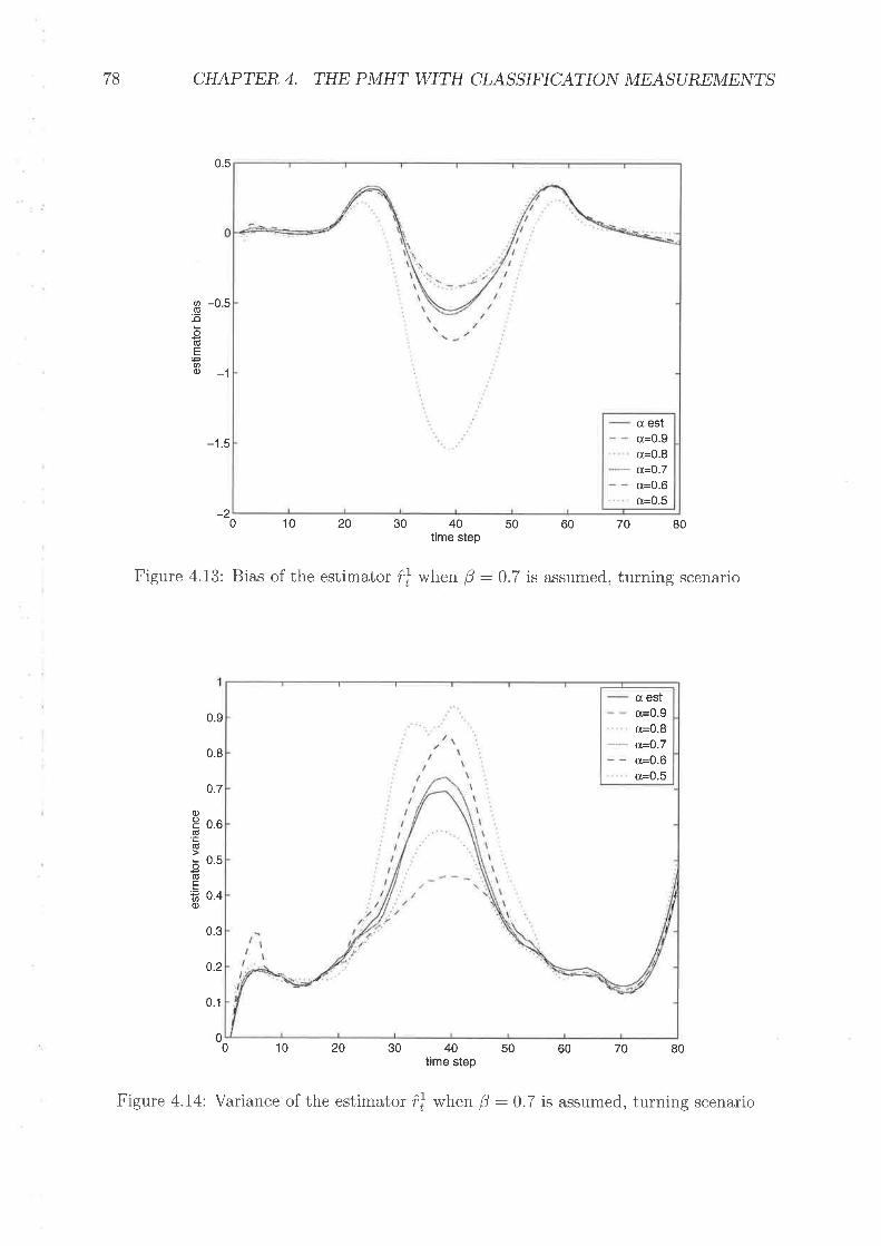
78 CHAPTER 4. THE PMHT WITH CLASSIFICATION MEASUREMENTS
-1
-1.5
-20 10 20 30 40
time step50 60 70 80
Figure 4.13: Bias of the estimator frl when þ :0.7 is assumed, turning scenario
05
v).q-o
(úEu,o)
-05
ooC.g(ú
o(úEU)(l)
0.9
0.8
0.7
0.6
0.5
0.4
0.3
0.2
0.1
00 10 20 30 50 60 70 8040
time step
û, esta=0.9u=0.8a=0.7o=0.6o=0.5
cx esta=0.9s=0.8cr=O.7ct=0.6o,=0.5
Figure 4.I4: Variance of the estimahor îl when 13 :0.7 is assumed, turning scenario
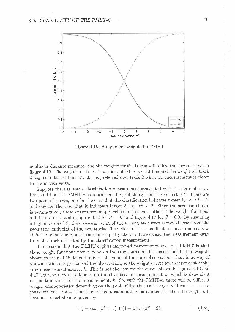
4.5. SENSITIVITY OF THE PMHT-C
0.1
79
0.9
0.8
0.7U'
ie o.o(l)È
Ë o.sEO)'6 0.4U)(ú
0.3
0.2
0-5 -4 -3 -2 -1 01state observation, zx
2345
Figure 4.15: Assignment weights for PMHT
nonlinear distance measure, and the weights for the tracks will follow the curves shown infigure 4.15. The weight for track l, u)t, is plotted as a solid line and the weight for track2, u2, as a dashed line. Track 1 is preferred over track 2 when the measurement is closerto it and visa versa.
Suppose there is now a ciassification measurement associated with the state observa-tion, and that the PMHT-c assumes that the probability that it is correct is p. There aretwo pairs of curves, one for the case that the classification indicates target 1, i.e. zk : I,and one for the case that it indicates target 2, i.e. zk : 2. Since the scenario chosenis symmetrical, these curves are simply reflections of each other. The weight functionsobtained are plotted in figure 4.16 for 0 : 0.7 and figure 4.17 for þ : 0.9. By assuminga lrigher value of B,lhe crossover point of the ?.u1 and ür2 cürv€s is moved away from thegeometric midpoint of the two tracks. The effect of the classification measurement is toshift the point where both tracks are equally likely to have caused the measurement awayfrom the track indicated by the classification measurement.
The reason that the PMHT-c gives improved performance over the PMHT is thatthese weight functions now depend on the true source of the measurement. The weightsshown in figure 4,15 depend only on the value of the state observation - there is no way ofknowing which target caused the observation, so the weight curves are independent of thetrue measurement source, k. This is not the case for the curves shown in figures 4.16 and4.17 because they also depend on the classification measurement zk which is dependenton the true source of the measurement,, k. So, with the PMHT-c, there will be differentweight characteristics depending on the probability that each target will cause the classmeasurement. If k : I and the true confusion matrix parameter is a then the weight willhave an expected value given by
1t.)t : alt)t (t* : t) + (t - o)wt (.r : Z) . (4.64)
1_. w2

80 CHAPTER 4. THE PMHT WITH CLASSIFICATION MEASUREMENTS
U'-c.9o3c0)E.s)U)U)(ú
0.9
0.8
0.7
0.6
0.5
o.4
0.3
0.2
0.1
0.9
0.8
0.7
0.6
0.5
0.4
0.3
0.2
0.1
0
Figure 4.16: Assignment weights for PMHT-c when 0 :0.7
-5 -4 -3 -2
-5 -4 -3 -2
-1 01state observation, zx
-1 01state observation, zx
2345
234
(t-c.9)oÈcoE.?.hth(ú
0
xk=1xk=1xk=2xk=2
ffft
wzwrwz
-w1
xk=1xk=1xk=2xk=2tW,
-w1 if
- w2ifwif
1
Figure 4.17: Assignment weights for PMHT-c when þ :0.9
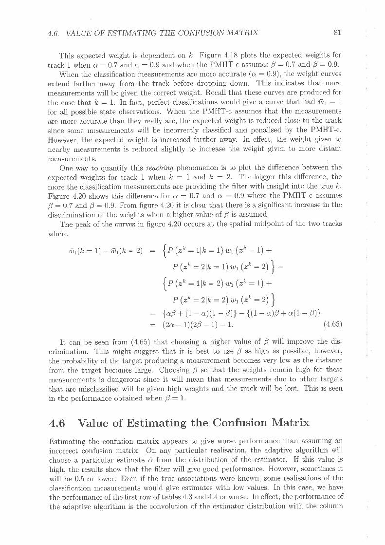
4.6. UALUE OF ESTIMA?IAIG THE CONFUSIO¡ú MATRIX 81
This expected weight is dependent on k, Figure 4.18 plots the expected weights fortrack 1 when a :0.7 and o : 0.9 and when the PMHT-c assumes 13 :0.7 and B : 0.9'
When the classification measurements are rnore accurate (a:0.9), the weight curvesextend farther away from the track before dropping down. This indicates th.at moremeasurements will be given the correct weight. Recall that these curves are produced forthe case that k: 1. In fact, perfect classifications rn'ould give a curve that had wt:1for all possible state observations. When the PMHT-c assumes that the measutementsaïe more accurate than they really are, the expected r,veight is reduced close to the tracksince some measurements will be incorrectly classified and penalised by the PMHT-c.However, the expected weight is increased farther away. In effect, the weight given tonearby measurements is reduced slightly to increase the weight given to more distantmeasurements.
One way to quantify this reach'ing phenomenon is to plot the difference between theexpected weights for track 1 when k : I and k : 2. The bigger this difference, themore the classification measurements are providing the filter with insight into the true k.Figure 4.20 shows this difference for a : 0.7 and a : 0.9 where the PMHT-c assumes
þ:0.7 andlj:0.9. Fromfigure 4.20iI isclearthatthereisasignificantincreaseinthediscrimination of the weights when a higher value of p is assumed.
The peak of the curves in figure 4.20 occurs at the spatial midpoint of the two trackswhere
u1(lç : L) - u{k :2) : {, f*: llk : 1) l¡r (zk : t) +
P ("r :2lk : I) wt ("* : Ð\ -{pQ*:rlk:2)ut(zk:t)+t
P ("r :2lk :2) w, (.* : ù\: {*þ+ (t-a)(1 - P)) -{(1 -c-)13 +o(1 - P)}: (2* - L)(213 - 1) - 1. (4.65)
It can be seen from (4.65) that choosing a higher value of p will improve the dis-crimination. This might suggest that it is best to use B as high as possible, however,the probability of the target producing a measurement becomes very low as the distancefrom the target becomes large. Choosing p so that the weights remain high for thesemeasurements is dangerous since it will mean that measurements due to other targetsthat are misclassified will be given high weights and the track will be lost. This is seen
in the performance obtained when þ : l.
4.6 Value of Estimating the Confusion MatrixEstimating the confusion matrix appears to give worse performance than assuming anincorrect confusion matrix. On any particular realisation, the adaptive algorithm willchoose a particular estimate ô from the distribution of the estimator. If this value ishigh, the results show that the filter will give good performance. However, sometimes itwill be 0.5 or lower. Even if the true associations were known, some realisations of theclassifrcation measurements would give estimates with low values. In this case, we havethe performance of the first row of tables 4.3 and 4.4 or worse. In effect, the performance ofthe adaptive algorithrn is the convolution of the estitnator distribution with the column

82 CHAPTER 4. THE PMHT WITH CLASSIFICATION MEASUREMENTS
0.9
0.8
olõ 0.7EoE
þ 0.6U)E.9) 0.5o35 o.¿Ec.9E 0.3(ú
0.2
0.1
-4 -3 -2 -1 01state observation, zx
3452
Figure 4.18: Assignment weights for PMHT-c when a:0.7
09
r 07õc:06ØE3 0sIg
Ë o+Ê.9Ød 03
0.8
01
-4 _a -2 -1 U 3 4
state observation, zx
02
0
_ B=0.7Þ=0'9
_ p=0.7= 0.9
Figure 4.19: Assignment weights for PMHT-c when a:0.9
5
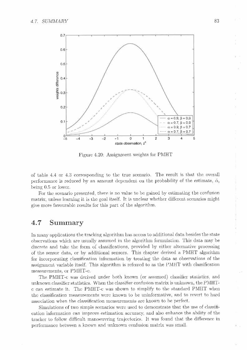
4.7. SUMMARY
0.7
0.6
0.5
o.2
0.1
o(Jco)(¡)
=E(t)
.9o)
=
40
30
0-5 -4 -3 -2 -1 01
state observation, zx
2345
Figure 4.20: Assignment weights for PMHT
of table 4.4 or 4.3 corresponding to the true scenario. The result is that the overallperformance is reduced by an amount dependent on the probability of the estimate, ô,being 0.5 or lower.
For the scenario presented, there is no value to be gained by estimating the confusionmatrix, unless learning it is the goal itself. It is unclear whether different scenarios mightgive more favourable results for this part of the algorithm.
4.7 SummaryIn many applications the tracking algorithm has access to additional data besides the stateobservations which are usually assumed in the algorithm formulation. This data may bediscrete and take the form of classifications, provided by either alternative processingof the sensor data, or by additional sensors. This chapter derived a PMHT algorithmfor incorporating classification information by treating the data as observations of theassignment variable itself. This algorithm is referred to as the PMHT with classificationmeasurements, ot PMHT-c.
The PMHT-c was derived under both known (or assumed) classifier statistics, andunknown classifier statistics. \Mhen the classifier confusion matrix is unknown, the PMHT-c can estimate it. The PMHT-c was shown to simplify to the standard PMHT whenthe classification measurements were known to be uninformative, and to revert to hardassociation when the classification measurements are known to be perfect.
Simulations of two simple scenarios were used to demonstrate that the use of classifi-cation information can improve estimation accuracy, and also enhance the ability of thetracker to follow difficult manoeuvring trajectories. It was found that the difference inperformance between a known and unknown confusion matrix was small.
83
- a=0.7, = 0.7
0.e, P = 0.9-- d=0.7,p=0.9
ct=0.9,9=0.7

84 CHAPTER 4. THE PMHT WITH CLASSIFICATION MEASUREMENTS
Similar simulations were also used to examine the change in performance when thePMHT-c assumed a confusion matrix which was incorrect. Surprisingly, it was shown thatthe performance actually improved in many cases when an overly optimistic confusionmatrix was assumed. This occurs because the PMHT-c with an optimistic confusionmatrix gives more emphasis to the classification measurements. Provided that they arecorrect most of the time, this implies that the algorithm emphasises the correct assignmentdecision, and performance is improved.

Chapter 5
A Dynamic Model for MeasurementAssignment the ProbabilisticMulti-Hypothesis Tracker withFlysteresis
A key feature of the PMHT algorithm is the unique way in which it models the as-
lì. signment of measurements to the dynamic state models used to represent targetsand clutter. The PMHT assumes that the true source of each measurement is a randomvariable. Each measurement has an assignment random variable which is independent ofthe assignment of other measurements, given that the probability mass is known. Whenthe assignment probability mass is unknown, it can be estimated by the PMHT.
Under the standard PMHT formulation [SL95], the probability mass of the assignmentvariable is assumed to be either time independent, or fixed over the batch. This is ratherlimiting, and it may be useful to adopt a model where the assignment probability evolvesaccording to a probabilistic process.
This chapter presents a ner,¡/ extension of the PMHT which incorporates a state modelfor the assignrnent prior and hence allows for its dynamic evolution. That is, a Bayesianhyperparameter for the assignment process is introduced, and this hyperparameter istreated as a random process. This model is shown to be a generalisation of the stan-dard PMHT assignment model. Two alternative approaches are identified for solving thegeneralised assignment model, and algorithms derived for each approach.
5.1 The Standard PMHT Measurement AssignmentModel
The main difference between the PMHT algorithm and other tracking approaches is theassumed measurement model from which the algorithm arises. Under the usual measure-ment model, there is an assumed prior processing stage that ensures that every targetpresent produces, at most, one measurement. If the target is distributed over severalsensor bins, a quasi sufficient statistic is assumed to be achieved through locating thepeak of this distributed response, or alternatively its centroid, or some other summarisingpoint. The result of this assumption is that there is, at most, one measurement belongingto each track. This makes the track to observation association process dependent becausethe assignment of one observation may alter the possible assignment options for the next.
85

86 CHAPTER 5, THE PMHT WITH HYSTER.ESIS
(a) standard measurement model (b) PMHT measurement model
Figure 5.1: Measurement Model BINs
The PMHT uses a different model, inspired by viewing the measurements as a col-lection of independent observations of a mixture. The PMHT assumes that the trueassignment of each neasurements is an independent random variable with a possible un-known prior probability mass function. The result of this assumption is that the track toobservation association is independent for each different observation. This independenceis the cause of the PMHT's linear complexity in the problem size, and allows the PMHTto perform batch processing, which is otherwise unfeasible due to the prohibitive growthin computational requirements under the standard model.
The difference between the assumed measurement process for the standard trackingparadigm and the PMHT is highlighted by the Bayesian Inference Networks (BINs) shownin figure 5.1. Each random variable is represented by a circle in the BIN and the arrowslinking the circles show the conditional dependence of the variables. In the figure, thereare two target models, and n¡ measurements. Under the standard tracking measurementmodel, there is an assignment variable for each target model, and all measurements aredependent on it. For the PMHT model, there is different assignment for each measure-ment. Under the standard model, all measurements must be used to jointly estimateeach assignment. Under the PMHT model, each measurement is used independently toestimate the single assignment variable associated with it.
As introduced in section 3.2.7, the prior probability mass of the assignment takinga value m, P(krr: m), is denoted by n?. The ri values are constrained to sum tounity over rL (by the law of total probability). Under the standard PMHT, the nl areeither known, or obey restrictive assumptions: they must be constant over fixed intervalsand independent between intervals. These assumptions are usually simplified to makethe priors constant over the batch, or independent from scan to scan. These restrictiveassumptions will now be relaxed, and the probability mass will be assumed instead to obeya state model, with the state evolving randomly with time, i.e. the r! are assumed to bea random process. The resulting algorithm is referred to as the PMHT with hysteresis,since the state model for assignments produces a temporal dependence in the assignmentprior probability.

,I-t
lvI v* t-7
"!!,
r!
l\I wîl ztt Iett
Zt, kn dI
-AI d,yt "
ztn! letnr
dI_,
dy{
5.2. ASSIG¡úMENT STATE MODEL
scan ¿- 1
scan ¿
87
scan t- 1
Figure 5.2: BIN for PMHT with hysteresrs
5.2 Assignment State ModelThe remainder of this chapter will deal with a problem deflnition expanded from thatin chapter 3. The standard PMHT observer was reviewed in chapter 3, and consists ofthe model states, and the assignments. Here the observer is extended to also containa further random variable, that acts as a state variable for the assignments. It will beassumed that a subset of the models have time dependent assignment probabilities. Theothers are independent, conditioned on the dependent priors (since normalisation links allof the priors). Those models that have time dependent assignment probability each havean associated assignment state. The assignment state for model m at scan t is dl, and itdefines the assignment prior probability for that model, i.e. di is a hyperparameter. df is
a scalar. It will be seen to be convenient to choose the assignment state to be discrete (inorder to achieve a problem solution). However, this is not a fundamental property of thehysteresis model and this choice will be deferred until the algorithm solution is obtained.
Define the per scan set Dt = {¿i.. d,y"} and the batch set D = {Do...Dr}'The assignment state is assumed to be a first order Markov random process with knownevolution probability density (or mass) function LT @Tld?r). th" prior distribution forthe assignment state of each model is also assumed known and is denoted as Aff (dfi').
Figure 5.2 shows a one scan slice of the Bayesian Inference Network (BIN) for thePMHT with hysteresis. The BIN demonstrates how the assigument state variables pro-vide a dynamic model for the probability mass of K. This dynamic model is the keycontribution of this chapter.
Assume that the number of measurements due to targets is relatively low comparedwitir the number of measurements due to clutter. This implies that the mixing proportionsassociated with target models, rl for m: My +1...M, are low compared with thosefor the clutter models, rl for rn : L . My While this assumption is valid for many

88 CHAPTER 5. THE PMHT WITH HYSTERESIS
tracking systems, it may not necessarily be the case.The assignment state is the underlying random process that determines the ri. It
will be assumed that the dependence of fI¿ upon D¿ takes the form:
óT-n" (¿T-r*) m) My,
ri (Dr): NIx (5. 1)
oi 1- t óî@,Ð 0<m1My,
where the functiottt df @'r) are assumed to be known, and the parameters øfl are therelative mixing proportions of the clutter models, which are assumed to be unknown.The oi represent the prior probability that a measurement is due to clutter model rngiven that it is due to clutter, and are constrained by
0{o!17, (52)tuJY
Ð"i : t. (5 3)m,:7
Define the sets E, : {ol...oy"i and Ð : {Xr...Xr}.The functions /f (df ) represent probabilities and so must be positive semi-definite
functions, namely they may not give negative values for any di. (5.1) ensures that the n'flsum to unity for any values of óï @í), provided that the constraint (5.3) holds. However, ifsome of the þi (df) take values that are too large, then some of the ri wrll not correspondto legal probabilities. For example, if the sum of the þi (df ) is greater than unity, theclutter priors will be negative. This is why it is necessary to assume that the number ofmeasurements due to targets is low. This assumption then corresponds to constrainingthe maximum values of each of the ó', (d,Ð to be sufficiently low to ensure that the rl arepositive.
It is possible to use a different definition for the dependence of the priors on the D,rather than (5.1). A general form, such as assuming rT : óT@t) could be used. Theform in (5.1) was chosen because it concentrates the joint dependence of fI into onìy theclutter models. The target n fl values are thus independent of each other. This may bedesirable if partial trM is used to reduce the complexity. This choice does not alter thealgorithm derivation, and a modified D dependence could easily be used.
The assignment state parameter will be assumed to occupy a finite discrete space.Without loss of generality, this space is assumed to contain Mp elements, with the as-signment state taking an integer value between 0 and Mo - I. The decision to use adiscrete assignment state parameter, rather than a continuous one, is driven by a de-sire to achieve at a soluble problem. For continuous random variables, the only optimalestimators known are those due to Kalman lKal60] and Benes [Ben81]. Each of theseaddresses a special case of the state evolution and observation equations. Both require alinear observation with Gaussian noise. In this problem, the functions Afl (a7la7r) anaóT @T) are the evolution and observation functions respectively. To achieve the positivedefinite constraints, and an upper bound, means that these functions cannot adhere tothe Kalman or Benes formulations. Thus, no continuous functions will give rise to anoptimal solution (barring the discovery of another continuous optimal filter, which wouldbe a major contribution of itself).
The particular forms of the functions óT @,n and Afl (Afl¿yr) are chosen accordingto the specific problem to be solved. The PMHT algorithms derived in this chapter are

5.2. ASS/GNME¡íT STATE MODEL 89
applicable for any functions, when di \s discrete. This is because discrete problems aresolved in a direct numerical manner by algorithms such as the Viterbi algorithm, or theHidden Markov Model Smoother, without the problematic analytic integration requiredfor optimal solution of continuous problems
5.2.L A Note on TerminologyThe hysteresis model is somewhat similar to a model used originally with the PDAFfor track initiation. For historical reasons, this model is variously referred to as targetobseruab,ilttE, track eristence, null track, target percei,uabi,h,ty, and target ui,si,bi,li,ty (e.g.
[CDA86, \,{8594, LL01a, Col99]). These various names all apply to the same approach(with minor variations on the theme) and are collectively described here as visibility. Thepurpose of visibility is to provide an integrated model specifically designed for makingtrack decisions, such as those for automated initiation and termination of tracks.
In the PDAF context, visibility is a binary attribute of targets that controls whether ornot they are able to be detected. A u'is'ible target provides a signal at the sensor which may(or may not) be detected, whereas an'inu'is'ible target cannot be detected. An exampleof an invisible target, is one occluded from the sensor due to physical constraints, suchas blind doppler zones, or the physical extent of the sensor region. Targets may becomeinvisible due to a manoeuvre (for example an aircraft might land) or simply by leavingthe footprint of the sensor. Tracks started on clutter measurements may be consideredto be due to postulated fictitious invisible targets. Hence the model incorporates bothdetectability and existence.
The visibility model is not restricted to the PDAF, but is rather an alternative statemodel for targets. This model has been used in various other filters, such as the GaussianSum Filter [R400], the Viterbi Algorithm [PL97], and with Random Sets |CVWO2].
The framework of the PMHT with hysteresis can be viewed as a generalised version ofvisibility. The simplest case of the hysteresis model is when the assignment state variableis chosen to be binary. In this case, the PMHT with hysteresis simplifies to the PMHTwith visibility when the appropriate dependence of fI on D is chosen. This model will bediscussed in more detail in chapter 6 when the PMHT with hysteresis is applied to trackinitiation.
Whereas visibility is a binary random variable with a fixed effect on the detectability ofa target, the assignment state model used for the PMHT is a general Markov process withan unspecified dependence on the prior assignment probability mass, fL The assignmentstate acts as a state of a general dynamics model for the assignment prior. Of course,particular models must be assumed to arrive at an implementable algorithm, but thePMHT formulation is not restricted to these forms.
In contrast to PDAF implementations of target visibility, the interpretation of thehysteresis model with PMHT is well defined and not contentious. In the PDAF com-munity, the physical interpretation of visibility has been a source of some consternationamong researchers, with various claims made about which interpretation offers the mostcomplete theoretic description.
The term ui,si,bi,li,ty is not used to describe the PMHT with Hysteresis because theextended assignment model is much more general than the problem of track initiationand termination addressed by the visibility model. The PMHT with Hysteresis is afundamental generalisation of the standard PMHT, of which automated track decisionmaking is merely an application.

90 CHAPTER 5, THE PMHT WITH HYSTERESIS
5.2.2 PMHT \Mith HysteresisThe PMHT with hysteresis is derived in substantially the same way as the standardPMHT. The derivation of the PMHT has been given in more detail in chapter 4 where thePMHT-c algorithm was derived. Therefore, the derivation of the PMHT with hysteresisis merely outlined here, although detail is given where it deviates from the derivation inchapter 4. The symbols used in this derivation were defined in chapter 3.
There are two approaches that can be used to develop an algorithm based on thismodel. Firstly, the assignment state can be treated as further missing data in an EM con-text. This means that the auxiliary function will be the expectation over the assignments,K, and the assignment states, D.ln this case, the algorithm will be seen to calculate theprobabilities of the dl, much as the standard PMHT calculates the probabilities of theassignments, k¿, (these are the weights, umtr).
The second method of solution is to estimate the assignment states. In this case,the auxiliary function becomes a function of the target states and the assignment states,dependent on their values frorn a previous iteration. Under this approach, the assignmeutstate is treated in a similar \May to the target state estimates. An initial assignment statesequence is assumed, and this sequence is iteratively refined based on the measurementassignment weights.
Each of the above approaches will now be explored, and PMHT algorithms derived.The algorithm resulting from treating the assignment states as missing data will be re-ferred to by the notational shorthand PMHT-ym. Similarly, the algorithm resulting fromestimation of the assignment states will be referred to as PMHT-ye.
5.3 Hysteresis as Missing Data, PMHT-ymOne way to derive an algorithm with the expanded measurement model incorporatinghysteresis is to treat the assignment state variables as additional missing data. Thisapproach is now considered. The algorithm derived through this approach is referred toas the PMHT-ym.
The missing data is now the assignments, and the assignment states. This means thatthe auxiliary function will be the conditional expectation over the assignment states, andthe assignments. Namely,
I (x,tlx(t), t(n)) : I Ito*P(x, D,K,z)P(D,Klxr'l,2), (5 4)DK
where the summation denot"d t is the sum over all possible permutations of the assign-
ment states, D. Explicitly,D
Mp-7 Mp-I:t tdå:o a2o:o
{}tD
Mp-| IvIp-I Mo-It t t{}a{x:s a!:o aY*:o
(5 5)
The BIN in frgure 5.2 illustrates the independence assumptions of the filter. Theseassumptions are that the state models are independent of each other and that the assign-ment states are independent of each other. Under these assumptions, the complete dataIikelihood is
p(x, D,K,z): p(x)p(D)p(KlD)p(zlK,x). (5 6)
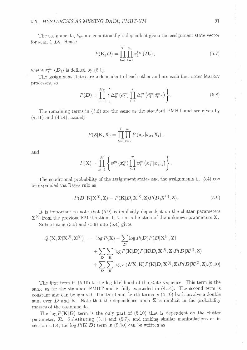
5.3. HYSTERES/S AS MISSI¡\IG DATA, PMHT-YM 91
Tlre assignments, k¡¡, àrê conditionally independent given the assignment state vectorfor scan t, Dt. Hence
TntP(KID) : fI n "!* (D,) , (5 7)
t:I r:l
where lTf* (Dù is defined by (5.1).The assignment states are independent of each other and are each first order Markov
processes, so
P(D): fI ^T @,n lI ¡r @Tt¿\,)
Ms¡
m:l
DK
DK
T
t:l(5.8)
The remaining terms in (5.6) are the same as the standard PMHT and are given by(4.11) and (a.14), namely
TntP(zlK,X) : II il P (z¿,lk¡,,x¿),
and
t:I r:1
D
P(x) :fr_{w øn\r, (*r@r)\
The conditional probability of the assignment states and the assignments in (5.4) canbe expanded via Bayes rule as
P (D,Klx{r), Z) : P (KlD,x{ù, z¡ e çolx@,2¡ (5 e)
It is important to note that (5.9) is implicitly dependent on the clutter parametersX(i) from the previous EM iteration. It is not a function of the unknown parameters Ð.
Substitutins (5.6) and (5.9) into (5.-t) gives
8 (x, ) lxt¿1, t(n)) : Iog P(X) + t Ios P(D) P(olx{i) ,z¡
+ t I to* P(KID)P(KID, x@,Z)P(olxØ,2¡
+ t I to* P(zlx,K)P(KlD, x(¿), z)P(Dlx,'),2).(s.to)
The first term in (5.10) is the log likelihood of the state sequence. This term is thesame as for the standard PMHT and is fully expanded in (4.14). The second term isconstant and can be ignored. The third and fourth terms in (5.10) both involve a doublesum over D and K. Note that the dependence upon X is implicit in the probabilitymasses of the assignments.
The logP(KlD) term is The only part of (5.10) that is dependent on the clutterparameter, X. Substituting (5.1) and (5.7), and making similar manipulations as insection 4.7.4, the logP(KlD) term in (5.10) can be written as

92 CHAPTER 5. THE PMHT WITH HYSTERESIS
t t rog P(KID)P(KID, x{ù ,z¡r1o1x@ ,z¡DK:tt ttlogP (k*lD,) P (KlD, X{ù, Z1 e lDlX@, Z)
Tnt
t:7 r:1DT
-\--LT
:\-/,t:lT
Knt
K1 r:lnt IVI
Dt r:l kb:IM
t:I Dt m:IT My
t:I Dt m:Ilvly
t I rogr!', (D) p(KtlD, ¡t';l ,z)p(DtlxrÐ ,z)
t t I ,o* rf* (D,) p(KtlD,xQ'),z)p(DtlxØ,2)
: t t t tosri (D,) t p(k* : mlD,x@,z)p(Dlxt'),2)nt
r:lnt
m:L
r-IIvIx
:tt I to* óT @,nl wç-+rø,v,(Dt)-r
t Iog øf * log 1-tóT@,7))] å
u"tr(Dt))"1r,¡*,o),2), (b 11)s:1
where wn¿ù(D) is defined as
w-t (Dt) : P(kr, : mlD,XØ,Z). (5.L2)
Note that wnh(Dt) is implicitly dependent on the iteration index, z, but this index issuppressed to somewhat simplify notation.
The terms involving óT@T) in (5.11) are constant, since they are summed over d!.So, the only term in (5.11) that is significant is the one involving af . Let
e,n=ä{.- "í¡ ,-,}, (5 13)
where
urntr : Ð.^r,(Dò P(DtlX(Ð,2)D
: Dr(rr, : mlD,x@,2¡eçDlx@,2) (5.14)D
Then, (5.11) can be written as
T
t t rog p(KlD)p(KlD,x{ù ,z¡elDlx{';) ,z) : Der^ r AN, (b.lb)D K t--7
where A6 is an irrelevant constant.The measurement term, logP(ZIX,K), can be simplified using the same process as
in section 414 and cai,Jil;il]^,",r.,r,x(i), .,p(Drx@,2)
DK M r nt (b.16): tIt\osi;f QnþT)umtr.m-1 t:l r:I
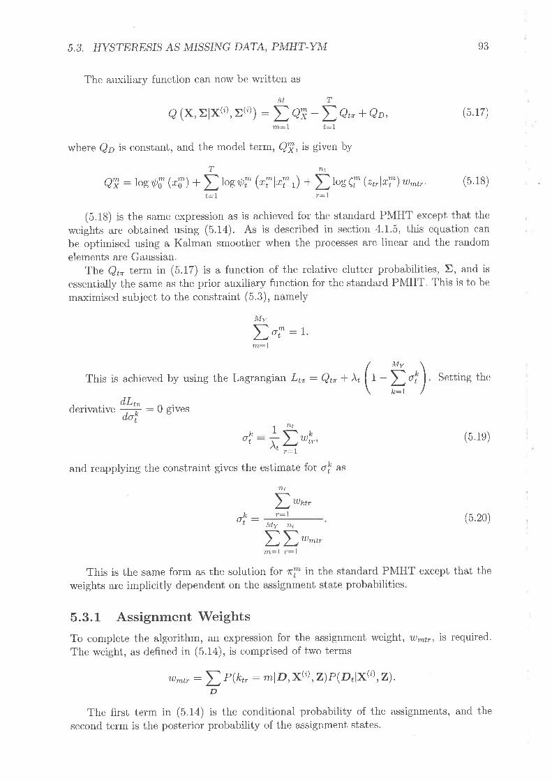
5.3. HYSTERESTS AS MISSI¡úG DATA, PMHT-YM
The auxiliary function can now be written as
lvl
93
(5.17)g (x,)lx{r),>(n)) : t eT +Dq^ t eo,n¿:7
T
t:7
where Qo is constant, and the model term, QT,i" given by
T TLt
QT : Iosrþi @i) + D to* ,þT @T1"7,) * D los (l Qr,lrT) u)m*. (5.18)t:l r:l
(5.18) is the sarne expression as is achieved for the standard PMHT except that theweights are obtained using (5.14). As is described in section 4.I.5, this equation canbe optimised using a Kalman smoother when the processes are linear and the randomelements are Gaussian.
The Q¡n term in (5.17) is a function of the reiative clutter probabilities, X, and isessentially the same as the prior auxiliary function for the standard PMHT. This is to bemaximised subject to the constraint (5.3), namely
My
ÐoT:tm:L
This is achieved by using the Lagran gian L¿n: Qtn+ i, (r -Ðrr)d,L,-
derivative É :0 gives
kot D'f,,
Setting the
(5. 1e)
(5.20)
1r¿t
Àf r:land reapplying the constraint gives the estimate lor of as
D'**nt
r:7o!: Mv nt
m:l r:7ÐÐ-^,,
This is the same form as the solution for rl in the standard PMHT except that theweights are implicitly dependent on the assignment state probabilities.
5.3.1 Assignment'WeightsTo complete the algorithm, an expression for the assignment weight, 'tt)*¡r, is required.The weight, as defined in (5.1a), is comprised of two terms
lnmtr : D, (rr, : mlD,x@,2) P (Dr1xØ, z¡.D
The first term in (5.14) is the conditional probability of the assignments, and thesecond term is the posterior probability of the assignment states.

94 CHAPTER 5. THE PMHT WITH HYSTERESIS
The conditional probability of the assignments is found via Bayes Rule
P (kr,: p¡¡(t) ,D,Z) : P (kr, - rn,xo), D,z)luI
s:1t r (kr, : s, x(i) , D,z)
P (x{;) , D,z\ rr) nT (Dr) Ç" (zr,l*i?t)M
I r (xt,l, D,z\ 2,,) nî (D,) ei (r"l*î,',)s:1
nT (D,) * (",,1*T'o')M (5.21)
I "¡ (D,) Ci (",,1*î,")
where Z\rr,is the set of all measur";;, in the batch except the measurement z¡,. (5.2L)is the same as the standard PMHT weight equation except that the prior distribution ofthe assignments, r! (D¿) is dependent on the assignment state D¿.
The posterior probability of the assignment state vector D¿ given all of the batchmeasurements and the state estimates at the previous iteration, namely P(DlX@,2),can be determined by using the Hidden Markov Model (HMM) smoother [JRS6].
Using Bayes Rule write
P (D'|X,Z) o( P (D1,X,Z): P (Dr, xl, xTr., z!, zTr): P (Dr,xi,zl) P (xlnr,zrr*rlor,xi,zi): a'(Dr) \r(D') =.yt(Dù , (5.22)
where
x:? : {Xr,...xr"}, (5.23)zii : {2r,... zr,} . (5.24)
The required probabilities are the y(D¡) and these shall be found be deriving recursiverelations for a¡(D¡) and p¡(D¿).
at(Dr) P (Dr, xi, zl)I r (Dr,Dr-r,xl,zi)Dt-t
\ e (DrlD,-1) p (x,lx¿- ù p (ztlD,, x,) att (D,-ùD+-t
I r (DrlDr-]) P (zrlDr,xr) ar¿ (Dr_)Dt-t
My
D lI ¡r @TøT') P (ZtlDt,Xr)rr-r (Dt-r) , (5.25)Dt-t rn:1
and a¿ (D¿) is normalised by dividine ¡V I ar(Dr)Dt
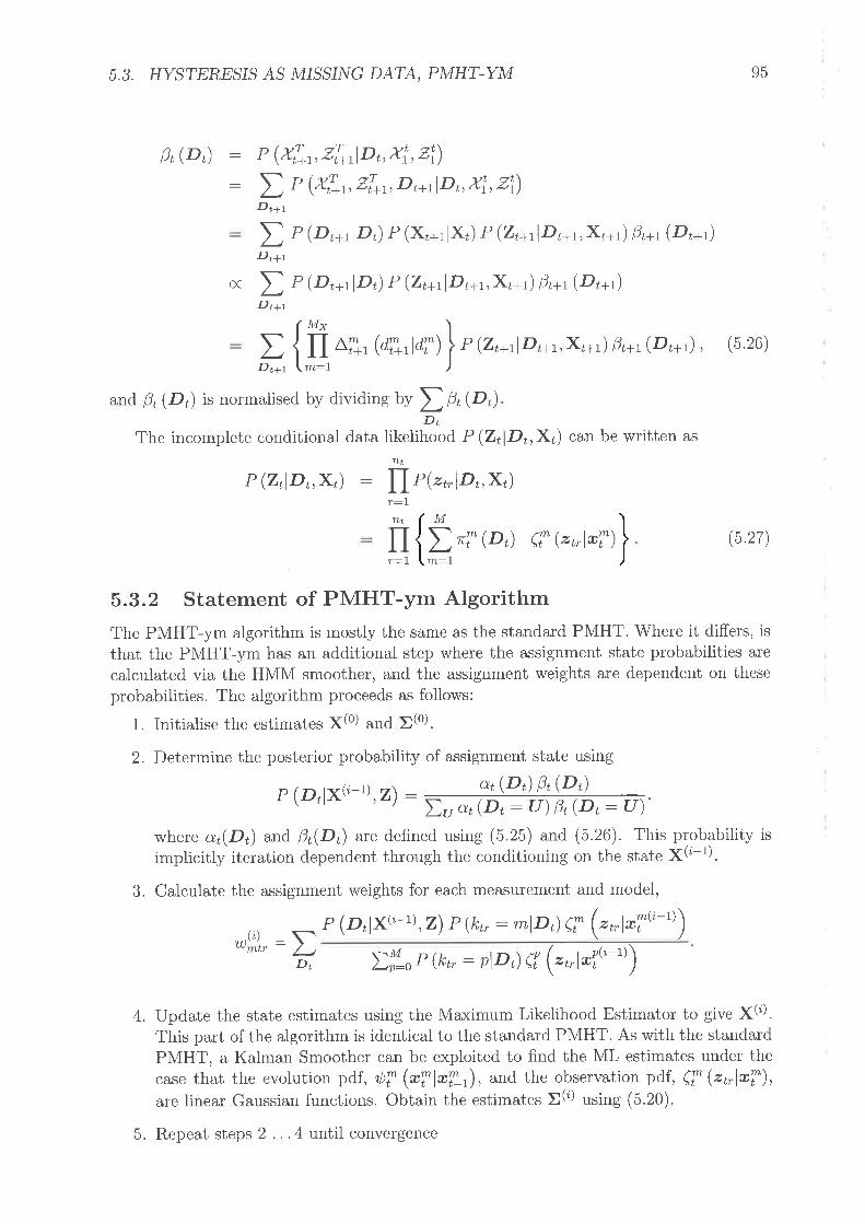
5.3. HYSTERESTS AS MISSI¡üG DATA, PMHT-YM
ílr(Dr) : P (XT*r,ZTrlDt,Xl,Z!): t r (xl*r, z{*r, Dr¡1lDb xl, z!)
Dt+t
95
(5.27)
t r (Dr*rlDr) p (x,*,.1x,) p (zr*rlDr+r, x,+r) þr+, (Dr+r)D r+1
o( \ e (Dr*,.lDr) P (zr+rlDr+r, Xr+r) l3r+, (Dr+r)Dt+r
p_ {ff, ^T*, (dr*,lor)
} p (2,*',1D,+,, x,+') 0,+, (D,*,¡ , (b.26)
and. B¡(D¿) is normalised by dividing ¡v D þt (Dt)D¡
The incomplete conditional data likelihood P (ZtlDr,X¿) can be written as
P (zlDúXt) P(z¿,lD¿,X¡)nt
Tr:7rLtilr:1
M
D"T @ò e? Q,,l*T)rn:
6.3.2 Statement of PMHT-ym AlgorithmThe PMHT-ym algorithm is mostly the same as the standard PMHT. Where it differs, is
that the PMHT-ym has an additional step where the assignment state probabilities arecalculated via the HMM smoother, and the assignment weights are dependent on theseprobabilities. The algorithm proceeds as follows:
1. Initialise the estimates X(0) and E(0).
2. Determine the posterior probability of assignment state using
p (Dtlx(i-r),2\ :,, ?:,(D)=9:(?:L =-/ Duc"t(Dt:U)0r(Dt-U)where at(Dt) and B¿(D¡) are defined using (5.25) and (5.26). This probability is
implicitly iteration dependent through the conditioning on the t¡u¡" ¡(t-t).3. Calculate the assignment weights for each measurement and model,
r (t,¡xt,;-r),2) P (kr, : *lDr) Ç (zt læitt'-tl),n,:ÐD¿ Ðy:, P (kr, : PlDt) Ç (.r,@Iþ-1))
4. Update the state estimates using the Maximum Likelihood Estimator to give X(¿).This part of the algorithm is identical to the standard PMHT. As with the standardPMHT, a Kalman Smoother can be exploited to find the ML estimates under thecase that the evolution pdf, ,þT@Tl*7.,), and the observation pdf, eTQ*l*T),are linear Gaussian functions. Obtain the estimates X(i) using (5.20).
5. Repeat steps 2 . . .4 until convergence
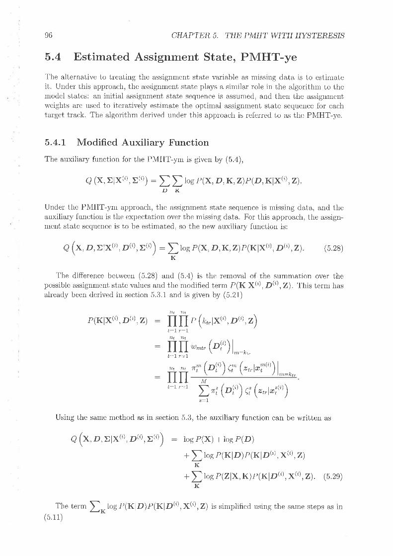
96 CHAPTER 5. THE PMHT WITH HYSTERESTS
5.4 Estimated Assignment State, PMHT-yeThe alternative to treating the assignment state variable as missing data is to estimateit. Under this approach, the assignment state plays a similar role in the algorithm to themodel states: an initial assignment state sequence is assumed, and then the assignmentweights are used to iteratively estimate the optimal assignment state sequerlce for eachtarget track. The algorithm derived under this approach is referred to as the PMHT-ye.
5.4.L Modified Auxiliary F\rnctionThe auxiliary function for the PMHT-ym is given by (5.a),
8 (x,)lx(r), t(o)) : I I to* P(x, D,K,z)P(D,xlx@ ,z¡DK
Under the PMHT-ym approach, the assignment state sequence is rnissing data, and theauxiliary function is the expectation over the missing data. For this approach, the assign-ment state sequence is to be estimated, so the new auxiliary function is:
O (*,D, tlx(i) , DØ) ,t(')) : I,o* p(x, D,K,z)p(Klx(t) , p(t') ,z) (5.28)K
The difference between (11.28) and (5.4) is the removal of the summation over thepossible assignment state values and the modified term P(KlX(t) , Dþ) ,Z). This term hasalready been derived in section 5.3.1 and is given by (5.21)
P(KlX(i) , D@,2) il il, (r,,¡xtt'), ntt),2)nt nt
t:l r:7
t:I r:7
nt ntilil ,^* (rÍn')l_:o"t:l r:7nt ntiltl "f (oÍ") eT (2,,1*i'o')1,_:*,.
M
D"; (rj") ei (',,¡'i'n')s:1
Using the same method as in section 5.3, the auxiliary function can be written as
O (*,D, Ðlx(r), p(r), ¡(r)) log P(X) * Iog P(D)
+ t log P(KID)P(KID@ ,x@,2¡K
+ t tog P(zlx, K)P(K|D@ ,x@ ,z). (b.2e)K
The term(5 11)
I*to* P(KlD)P(X¡ptol,X(i),2) is simplified using the same steps as in
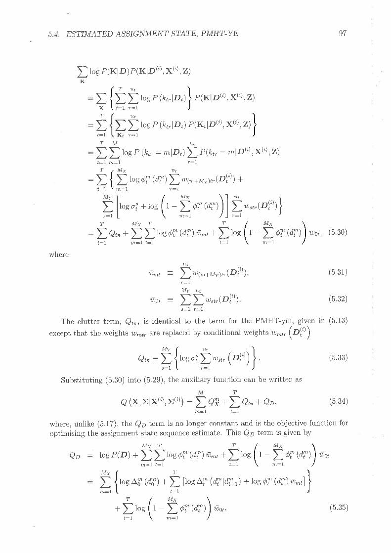
5.4. ESTIMATED ASSIG¡\TME IT STATE, PMHT-YE
I to* P (KID) P(x¡¿¡t';l,xØ,2¡
t:l
My
m:l
97
K
tKTt
t:lTt
t:1Tt
t:l
TLt
ttlogP (k*lD') P(KID@,X@,2)T
nt
r:L
I to* óT @,nr].ç***,v,(nÍo)) +
I to* P (kr,lD) P(KtlD(.o),x@ ,Z)
t:I r:lnt
r:7Mt
m:7log P (kr, : mlDr)D r(rr, : 72lPØ ,Y(t') ,z)
s:1T
Ms
m:1.
l.-
nt
r:I
T
t:lMy
rn:7
Mv Myt o.; + log 1- t óT @,7))] å,,,.@Ío\\T AIx
t:7 m:7
T
: t Q,n +t t roeÓT @T) ø*,+ ! log 1- t óT @,7) .u.ot, (5.30)m:l t:7
MvT
MxT
m,:7 t:I
t:lwhere
nt
wmt : lwç^+rør¡r,(DÍo)),
,rrr(Dlo))
The clutter term, Qrn, is identical to the term forexcept that the weights 'trp¡¡ àtE replaced by conditional
(5.31)
(5 32)
the PMHT-ym, given in (5.13)
weights .^r, (oÍo))
--1
Mv nt
wot: Its:l r:1
(5.33)
Substituting (5.30) into (5.29), the auxiliary function can be written as
Tg (x,rlx(r), r(o)) : t eT +Ðq^ t Qo, (b.34)
m:l t:l
where, unlike (5.17) ,the Qp term is no longer constant and is the objective function foroptimising the assignment state sequence estimate. This Q¿ term is given by
e,n =ä {.- "i¡,,,,, (rÍ',) }
Qo : log P(D) + t I to* óT @,n w^t * I to* 1- I óT @,7)
M¡trn:7
rog A,[" @Ð + I |to* LT @Tld\,) + toe öT @,7) ø*,)
T
+llog 1-tóT@,7)t:I m:l
uot
lxot
(5.35)
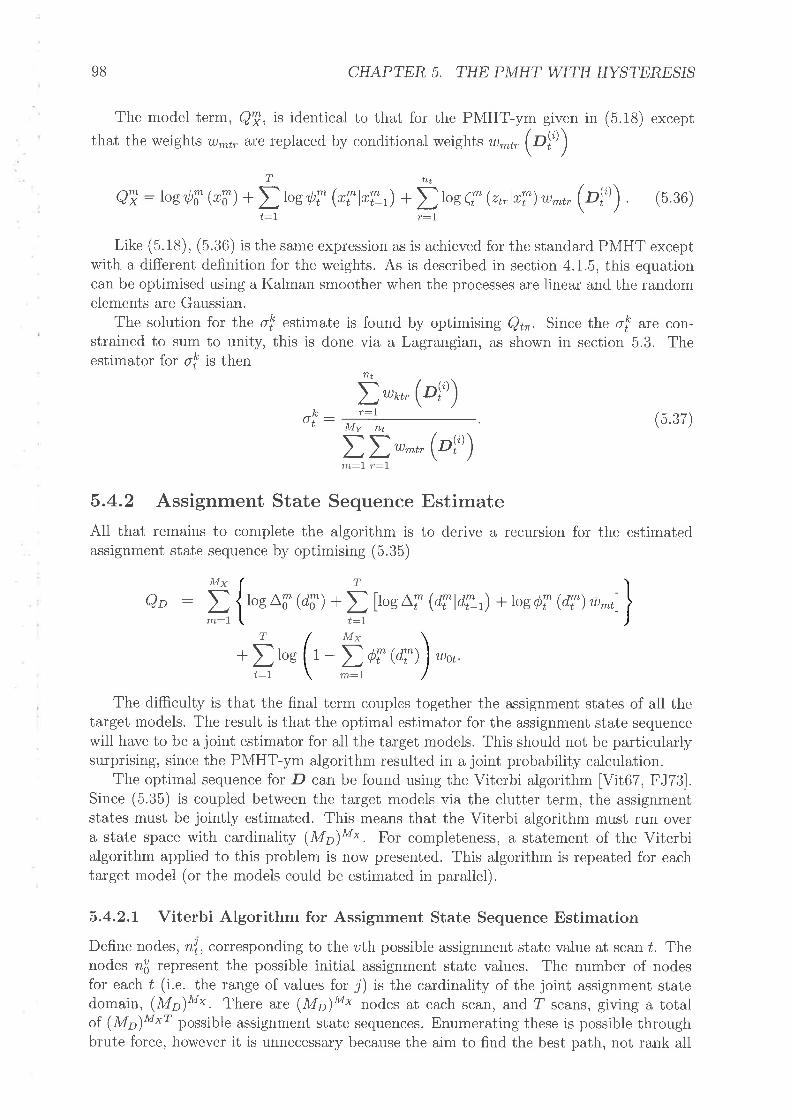
98 CHAPTER 5. THE PMHT WITH HYSTERESIS
The model term, 8T, i" identical to that for the PMHT-ym given in (5.1S) exceptthat the weights 'u)r¡1¿y àr€ replaced by conditional weighLs,u)^¡, (Ojt')
TntQT : I"srþi @i) + f ,o* ,þT (*Tl*7,) * I los (l Q,,lrT).*,, (olo') . (b.36)
ú:1 r--7
Like (5.18), (5.36) is the same expression as is achieved for the standard PMHT exceptwith a different definition for the weights. As is described in section 4.1.5, this equationcan be optimised using a Kalman smoother when the processes are linear and the randomelements are Gaussian.
The solution for the o! estimate is found by optimising Qrn. Since the o! are con-strained to sum to unity, this is done via a Lagrangian, as shown in section 5.3. Theestimator for o! is then
nt
Ð'r,,('Í")-t - M, -
\v.ur ,/
t t ,** (oÍn')m:I r:1
5.4.2 Assignment State Sequence EstimateAll that remains to complete the algorithm is to derive a recursion for the estimatedassignment state sequence by optimising (5.35)
Ms¡
Qo t rogAff @Ð + D [to* LT @,Tldî!,) + tog óT @T)ø^,]T
t:IM1¡T
ú:1
m:1.
+flog 1- t óT @,7) wotrn:7
The difficulty is that the final term couples together the assignment states of all Lhetarget models. The result is that the optimal estimator for the assignment state sequencewill have to be a joint estimator for all the target models. This should not be particularlysurprising, since the PMHT-ym algorithm resulted in a joint probability calculation.
The optimal sequence for D can be found using the Viterbi algorithm [Vit67, FJ73].Since (5,35) is coupled between the target models via the clutter term, the assignmentstates must be jointly estimated. This means that the Viterbi algorithm must run overa state space with cardinality (Mo)'t". For completeness) a statement of the Viterbialgorithm applied to this problem is now presented. This algorithm is repeated for eachtarget model (or the models could be estimated in parallel).
5.4.2.L Viterbi Algorithm for Assignment State Sequence EstimationDefine nodes, nf , corresponding to the'uth possible assignment state value at scan ú. Thenodes nfl represent the possible initial assignment state values. The number of nodesfor each ú (i.e. the range of values for j) is the cardinality of the joint assignment statedomain, (Mo)*". There are (Mo)mx nodes at each scan, and ? scans, giving a totalof (Mp)M*? possible assignment state sequences. Enumerating these is possible throughbrute force, however it is unnecessary because the aim to find the best path, not rank all

5.4. ESTIMATED ASSIGNME¡\IT STATE, PMHT-YE 99
paths. Thus, some sequences can be discarded before they are fully enumerated, once itis apparent that they cannot be the best path.
The log likelihood of a particular sequence can be accumulated along the path dueto the Markov nature of the assignment state process - given dT, dT*t is independent ofall other di and its likelihood is known. Further, for a particular node, it is possible toconstruct the likelihood of all partial sequences after that node, independent of the partialsequence prior to the node. This means that if the best sequence passes through nodenrr,then it must consist of the best partial sequence leading from scan I T,o nr, and the bestpartial sequence from n!, to scan 7.
The Viterbi algorithm then operates by retaining only the best partial sequence leadingto each node for each scan. When the last scan is considered, then the best sequence ischosen from the best sequences leading to each final node. Effectively, each possible pathis considered, but only (Mp)&1* sequences need to be remembered instead of (MD)Mxr.
For each node, define a cost, qi, and, a path prr. The path for nodeni represents themost likely assignment state at f - 1 given that the assignment state at t is nrr. The costis the log likelihood of the most likely assignment state sequence leading to node nf .
The Viterbi algorithm proceeds as follows:
1. For each j, calculate the initial node costs given by
Myq:o: DIog Aff (¿i : "lo)
(5.38)m:l
2. Starting with ú : 1, and for each j determine the best palh pr, given by
Mypi : ars'''u,* | lqf-, + log ai @T = "!rld\, = "f-t)). (5.3e)
m:1
3. Calculate the node cost for each node at f given by
Ma
d, D lnf-,-r rog LT @,7 = n!,ld,i1= "f)lln:otrn:7
+ t w-¡losóT @,7 -- "!r) *'us¿ log 1-tóT@,T="!,) (5.40)NIx
m:l
My
m:l
4. Repeat steps 2 and 3 Ïor t:2. . .7.
5. Determine the most likely final assignment state by finding the node with the highestq+
br =arsmax lqå] . (b.41)
6. Determine the earlier assignment state values by following the path backwards fromt:Tt'ot:t
bF1:ft ln=oi. (5.42)

100 CHAPTER 5, THE PMHT WITH HYSTERESIS
5.4.3 Statement of PMHT-ye AlgorithmThe PMHT-ye algorithm is mostly the same as the standard PMHT. Where it differs,is that the PMHT-ye has an additional step where the assignment state sequence isdetermined via the Viterbi algorithm, and the assignment weights are dependent on thissequence.
The algorithm proceeds as follows:
1. Initialise the model state estimates,;ç(0), and the assignment state estimates, D(0).
2. Calculate the assignment weights for each measurement and model,
P kr, m, D -1)
Ðy:,, (kr, p D tP\¿ Zb
) er (.,,1*7ro
lrl<landz+-1, (5.43)
( (i- 1)
wl),,: t
(r-1)t
3. Update the state estimates using the Maximum Likelihood Estimator to give X(¿).This part of the algorithm is identical to the standard PMHT. As with the standardPMHT, a Kalman Smoother can be exploited to find the ML estimates under thecase that the evolution pdf, ,þT@Tl*7r), and the observation pdf, eTQr,læT),are linear Gaussian functions.
4. Using the Viterbi algorithm, update the assignment state estimates to give p(¿).
5. Repeat steps 2 .. .4 until convergence
5.4.4 Approximate PMHT-ye with Reduced ComplexityIn the derivation of the PMHT-ye, it is fairly clear that the necessity to jointly estimatethe assignment state variables arises from the coupling through the clutter term in (5.35).If this term can be decoupled, then it would be possible to independently optimise thedifferent models. This is appealing because the Viterbi algorithm must consider all pos-sible transitions in the state space, of which there are D2, where D is the number ofstates. Performing My parallel optimisations over a Mo sized space is far preferable toperforming one optimisation over a (Mr)** sized space.
It is not possible to achieve this decoupling. However, an approximate decoupling canbe achieved by using the Taylor series expansion of the logarithm
log(1 + z): z -ïu * 7"-a,J
which for small z, admits the approximation
log(1 *z)xz lrl<1 (5.44)
Notice that it has already been assumed in section 5.2.2 lhat Lhe þi (df ) are suffi-ciently small to preserve normalisation. This requirement is quite loose. Provided that theother values are very small, óT @T): 0.9 would still be acceptable. If this requirementis tightened such that
Ma
I ør @'T) < r, (5.4b)L=t

5.4. ESTIMATED ASS/G¡üME¡úT STATE, PMHT-YE
then (5.35) can be approximated by
101
(5.46)
Qo = t togAff (¿Ð + I [to* LT @Tld\,) + tos óT @T)r¡*,)Ms1
m:l
T
t:1.IVIx
- t óT @,7)m:1
T
uot
óT @,7)-*'exp lóT @T) øorl
+Tt
t:lMy
t:Lt IogAff (¿3') + I [.* LT @,T d,7,) +r"sóT @T)ø^, - óT @Ðúo,]
D,qr (5.47)rn:I
The advantage of this approximation is that each of the functions QB is now inde-pendent of all of the other models and the assignment state sequence for model m can beestimated independently of the other models. This means that the algorithm has linearcomplexity in the number of target models.
Let $i @i) be defined such that
: I"eóT @T).^, - óT @T) øor,
rn:IMy
ros þi @i)
ør r¿n
Then, Qfr can be written as
(5.48)
(5.4e)
Qß :rog Aff @Ð +I 1,"* ^T (dTld\,) + tog óf @,nl (5.50)
T
t:l
The function þi @i) is analogous to a measurement likelihood. If it were possibleto clroose óT @,?) such that óT @,7) is a Gaussian function, then the assignment statesequence could be estimated with a Kalman smoother. Howevet, the form of (5.a9)makes it impossible to frnd such a function for þi@i). In fact, it appears that thereis no function þi @i) that will result iu a closed form solutionl. However, (5.110) canbe optimised since di is a discrete random variable. As with the proper PMHT-ye,the assignment state sequence is now estimated with the Viterbi algorithm. Due to theseparation achieved through the approximation, each model is now optimised with anindependent Viterbi smoother.
5.4.5 Special Cases
In the previous chapter, the PMHT-c was seen to simplify to the standard PMHT whenthe classification measurements were known (or assumed) to be uninformative. Similarly,the PMHT-ye simplifies to the standard PMHT under special conditions. This kind ofbehaviour is not considered for the PMHT-ym, because it treats the prior in a differentway to the standard PMHT, which estimates it.
The transition probability, LT @TId\r), d"t.t-ines the main difference between thestandard PMHT and the PMHT-ym. The standard PMHT assumes the assignment
1It is the author's belief that no closed form solution exists. No attempt has been made to prove this,although it can be shown that there is no function óT @T) that results in a Gaussian ÓT @T).
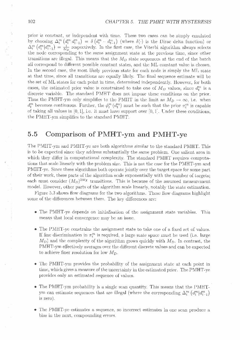
t02 CHAPTER 5. THE PMHT WITH HYSTERESIS
prior is constant, or independent with time. These two cases can be simply emulatedby choosing Af (Afl¿yr) : 6 (AT - d1r) (where ð(.) is the Dirac delta function) orLT @Tld!t) : # respectively. In the first case, the Viterbi algorithm always selectsthe node corresponding to the same assignment state at the previous time, since othertransitions are illegal. This means that Lhe Mp state sequences at the end of the batchall correspond to different possible constant states, and the ML constant value is chosen.In the second case, the most likely previous state for each node is simply the ML stateat that time, since all transitions are equally likely. The final sequence estimate will bethe set of ML states for each point in time, determined independently. However, for bothcases, the estimated prior value is constrained to take one of Mp values, since df is adiscrete variable. The standard PMHT does not impose these conditions on the prior.Thus the PMHT-ym only simplifies to the PMHT in the limit as Mo - oo, i.e. whendl becomes continuous. Further, the ó? (dT) must be such that the prior ri is capableof taking all values in [0,1], i.e. it must have support over [0, 1]. Under these conditions,the PMHT-ym simplifies to the standard PMHT.
5.5 Comparison of PMHT-ym and PMHT-yeThe PMHT-ym and PMHT-ye are both algorithms similar to the standard PMHT, Thisis to be expected since they address substantially the same problem. One salient area inwhich they differ in computational complexity. The standard PMHT requires computa-tions that scale linearly with the problem size. This is not the case for the PMHT-ym andPMHT-ye. Since these algorithms both operate jointly over the target space for some partof their work, these parts of the algorithm scale exponentially with the number of targets;each must consider (Mo)"t* transitions. This is because of the assumed measurementmodel. However, other parts of the algorithm scale linearly, notably the state estimation.
Figure 5.3 shows flow diagrams for the two algorithms. These flow diagrams highlightsome of the differences between them. The key differences are:
o The PMHT-ye depends on initialisation of the assignment state variables. Thismeans that local convergence may be an issue.
o The PMHT-ye constrains the assignment state to take one of a fixed set of values.If fine discrimination in ri is required, a large state space must be used (i.e. IargeMp) and the complexity of the algorithm grows quickly wiLh Mo. In contrast, thePMHT-ym effectively averages over the different discrete values and can be expectedto achieve finer resolution for \ow Mp.
o The PMHT-ym provides the probability of the assignment state at each point intime, which gives a measure of the uncertainty in the estimated prior. The PMHT-yeprovides only an estimated sequence of values.
o The PMHT-ym probability is a single scan quantity. This means that the PMHT-ym can estimate sequences that are illegal (where the corresponding LT (dTld\\)is zero).
o The PMHT-ye estimates a sequence, so incorrect estimates in one scan produce abias in the next, compounding errors.
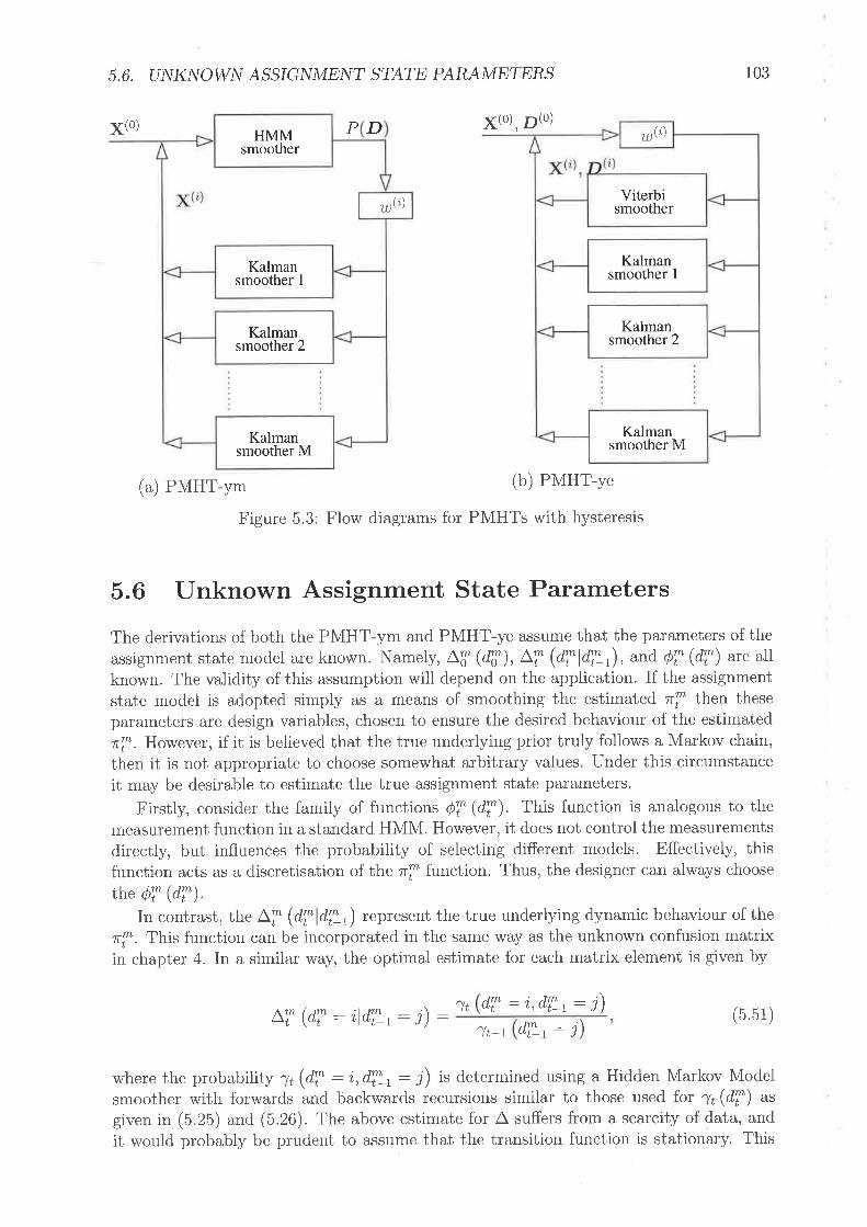
HMMsmoother
u)Q)
Kalmansmoother 1
Kalmansmoother 2
Kalmansmoother M
5.6. UNI(¡úOW¡ú ASSIG¡úME¡\IT STATE PARAMETERS 103
¡(o) P D ¡(o), p(o)
(a) PMHT-ym (b) PMHT-Ye
Figure 5.3: Flow diagrams for PMHTs with hysteresis
5.6 l-Jnknown Assignment State Parameters
The derivations of both the PMHT-ym and PMHT-ye assume that the parameters of theassignment state model are known. Namely, LT @,i), LT @Tld\r), and ó? (d'T) are allknown. The validity of this assumption will depend on the application. If the assignmentstate model is adopted simply as a means of smoothing the estimab,ed ri then theseparameters are design variables, chosen to ensure the desired behaviour of the estimatedzrfl. However, if it is believed that the true underlying prior truly follows a Markov chain,then it is not appropriate to choose somewhat arbitrary values. Under this circumstanceit may be desirable to estimate the true assignment state parameters'
Firstly, consider the family of functions óT @,7). This function is analogous to themeasurement function in a standard HMM. However, it does not control the measurementsdirectly, but influences the probability of selecting different models. Effectively, thisfunction acts as a discretisation of the ri function. Thus, the designer can always choosethe þi @i').
In contrast, the Af (Afl¿\) represent the true underlying dynamic behaviour of therfl. This function can be incorporated in the same rù/ay as the unknown confusion matrixin chapter 4. In a sirnilar way, the optimal estimate for each matrix element is given by
LT @,7 : ildTt: i) : ''lt dT : i,d\r: j)(5.5 1 )
'Yt-t d\r: j)
where the probability n (¿T : ù,dTt: ¡) is determined using a Hidden Markov Modelsmoother with forwards and backwards recursions similar to those used for y @i) as
given in (5.25) and (5.26). The above estimate for A suffers from a scarcity of data, andit would probably be prudent to assume that the transition function is stationary. This
u)Q)
Viterbismoother
Kalmansmoother I
Kalmansmoother 2
Kalmansmoother M

104 CHAPTER 5. THE PMHT WITH fIYS"ERES/S
leads to temporal averaging and the estimated A is then given by
T
Dl (¿T i,d7, )J
LT @,7 : i,ld\t: j) : T
l*-' (¿7r: i)t:7
(5.52)
The main application of the assignment state model considered in this thesis is as ameans for smoothing the nfl estimate. Thus, it will be assumed that the assignment stateparameters are known, since they are design choices based on the degree of smoothingdesired.
5.7 Simulated ExampleTo demonstrate the use of the PMHT-ym and PMHT-ye algorithms, a simple simulatedexample is now considered. The simulation consists of a two model scenario with staticstates, but varying mixing proportions. Multiple scalar measurements are detected ateach scan, and these are the only information provided to the tracker.
Each model has a two element state, defining the mean and variance of the (Gaussian)measurement density function for that model. Thus the state vector is
æT =¡m:1"*lltl,r^lo'lf', (b.b3)
and the measurement pdf is
t:I
Both models are chosen to have a variance of 2.25, i.e. rLl"'l - ,'lo'l - 2.25. Themeans are chosen as rrlp,]: 1 and ,'[tt]: -1. A batch length of T :100 is used withTLt:5 measulements per scan.
The mixing proportions of the two components vary sinusoidally such that
e^ Q*): (2trr*[o'])-å "*o
r¿1 : 0.5 - o.Jcos W)
(5.54)
(b.55.)
Thus the rl vary between 0.2 and 0.8, and there are / cycles of the sinusoid over thebatch. Two different frequencies are considered: f :1, and Í : 4. Figure 5.4 shows themeasurements from an example trial where f : I is used. It can be seen that there aremore rneasurements at high values when the first model dominates, in the middle of thebatch.
The mean and variance of the state estimate and the prior estimate are measured over1000 Monte Carlo trials. The PMHT-ym does not produce a prior estimate, but rathera probability mass for the prior. The mean of this probability mass is used as a priorestimate for the purpose of this comparison.
The performance of the PMHT-ym and PMHT-ye is compared with the standardPMHT which assumes that the prior probabilities are time independent.
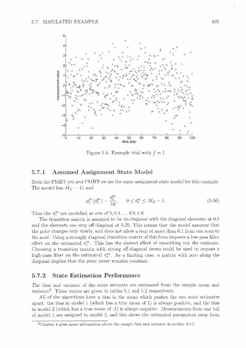
5.7. SIMULATED EXAMPLE 105
IX
5
4
óx x
X
X
X
X
X
X x
X
X
X X XXX.,
X XXXX
X
x X x
X
x
XXI
xxX x
XX XX
X
X x
Xx
XxX
x., x
x
Xxx
xx
xi
X
t",
X X
xx
X
x
x
X X
XX
X
X
,'*
x
X X( x
x X
X
XX
X
X
x
x
x
XX xxx"tXx
xXx X
2 X x
, "t
XxX xI& ,¿ç"x XX X
"" XX xX
X
*xx"x x
x
X
X
X
X
o(d
oEof.t)(ú0)E
X
X,\
X
XÁ & XXXx X*ç* g
x \"XXX
I
XXX
X
xtxx
xX¡X
x x
x X
X
X XX
¡xxxs.Xx xxx
X
x*x X "" t\]l
XX
0 x li"e x¡xx
XiðX
X
X
xxx xx
xX X
Xxxx x
xxu.- Xx xx ¡ ¡"& ¡'"
xXX
X* x x",
X5oX XX 56. x"tr XXx
xX
x\X X
X
*?l
WXXW"x ¡¡X¡X ¡'x \ øtx¡¡Xxx 4,
XX
x xx )¡XX &xx x'' x xxXX
"&t
X
\X ¡ X
X
*" *'x
gXxX ^xXx
XXXx
-2
-3
-4
-5
Xo""
XX X
XXXX
.Xxxxx XXx
Xxx XX
X xx X x X
X
x
10 20 30 40
xxX
X
X
0 50time step
60 70 80 90 100
Figure 5.4: Example trial with / : 1
5.7.L Assumed Assignment State ModelBoth the PMHT-ym and PMHT-ye use the same assignment state model for this example.The modelhas Mp: 11 and
dvtóT @n: ïb, o < dT < Mo - r' (5.56)
Thus the rl are modelled as one of 0,0.1, . . . 0.9, 1.0.The transition matrix is assumed to be tri-diagonal with the diagonal elements at 0.5
and the elements one step off-diagonal at 0.25. This means that the model assumes thatthe prior changes only slowly, and does not allow a step of more than 0.1 from one scan tothe next. Using a strongly diagonal transition matrix of this form imposes a low-pass filtereffect on the estimated zrfr. This has the desired effect of smoothing out the estimate.Choosing a transition matrix with strong off-diagonal terms could be used to impose ahigh-pass filter on the estimated ri. As a limiting case, a matrix with zero along thediagonal implies that the prior never remains constant.
5.7.2 State Estimation PerformanceThe bias and variance of the state estimate are estimated from the sample mean andvariance2. These values are given in tables 5.1 and 5.2 respectively.
AII of the algorithms have a bias in the mean which pushes the two state estimatesapart: the bias in model 1 (which has a true mean of 1) is always positive, and the biasin model 2 (which has a true mean of -1) is always negative. Measurements from one tailof model 1 are assigned to model 2, and this skews the estimated parameters away from
2Chapter 4 gives more information about the sample bias and variance in section 4.4.2
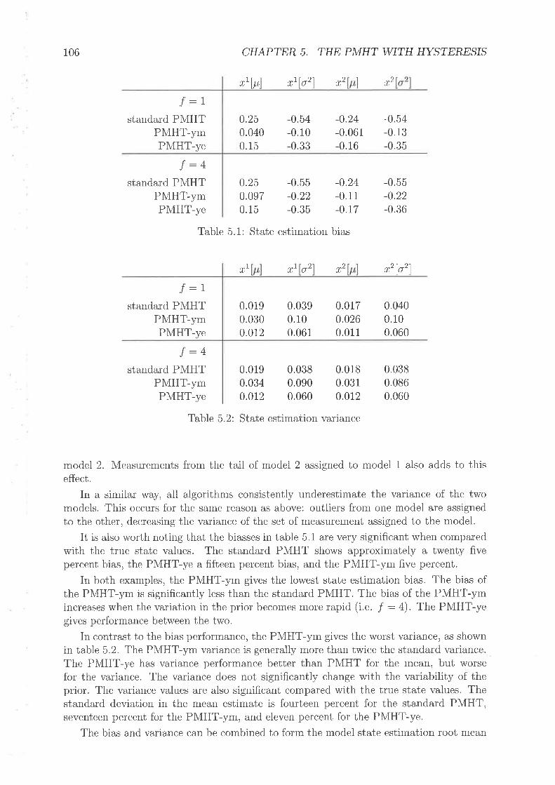
106 CHAPTER 5. THE PMHT WITH HYSTERESIS
,'ltl ,tlo'l 12 l,'I_1.t -L
standard PMHTPMHT-ymPMHT-ye
I_^J -+standard PMHT
PMHT-ymPMHT-ye
!_1J -Lstandard PMHT
PMHT-ymPMHT-ye
!_^J -+standard PMHT
PMHT-ymPMHT-ye
0.019 0.038 0.0180.034 0.090 0.0310.012 0.060 0.012
0.250.0400.15
0.250.0970.15
0.0190.0300.0r2
-0.54-0.10-0.33
-0.55-0.22-0.35
0.0390.100.061
-0.24-0.061-0.16
-0.24-0.11-0.r7
0.0170.0260.011
-0.54-0.13-0.35
-0.55-0,22-0.36
Table 5.1: State estimation bias
:LI rl o2 tT. t'lo'l
0.0400.100.060
0.0380.0860.060
Table 5.2: State estimation variance
model 2. Measurements from the tail of model 2 assigned to model 1 also adds to thiseffect.
In a similar way) all algorithms consistently underestimate the variance of the tw<r
models. This occurs for the same reason as above: outliers from one model are assignedto the other, decreasing the variance of the set of measurement assigned to the model.
It is also worth noting that the biasses in table 5.1 are very significant when comparedwith the true state values. The standard PMHT shows approximately a twenty fivepercent bias, the PMHT-ye a fifteen percent bias, and the PMHT-ym five percent.
In both examples, the PMHT-ym gives the lowest state estimation bias. The bias ofthe PMHT-ym is significantly less than the standard PMHT. The bias of the PMHT-ymincreases when the variation in the prior becomes more rapid (i.". / :4). The PMHT-yegives performance between the two.
In contrast to the bias performance, the PMHT-ym gives the worst variance, as shownin table 5.2. The PMHT-ym variance is generally more than twice the standard variance.The PMHT-ye has variance performance better than PMHT for the mean, but worsefor the variance. The variance does not significantly change with the variability of theprior. The variance values are also significant compared with the true state vaiues. Thestandard deviation in the mear estimate is fourteen percent for the standard PMHT,seventeen percent for the PMHT-ym, and eleven percent for the PMHT-ye.
The bias and variance can be combined to form the model state estimation root mean

5.7, SIMULATED EXAMPLE
1_1J -rstandard PMHT
PMHT-ymPMHT-ye
T-AJ -+standard PMHT
PMHT-ymPMHT-ye
r07
rI
0.290.180.19
ir+
r2lÀ ,'lo'l
0.29 0.58 0.280.2t 0.37 0.2r0.19 0.42 0.20
r'lo
0.580.330.47
0.270.770.19
0.580.340.43
0.580.370.44
Table 5.3: State estimation RMS error
square (RMS) error, represented by e. The estimated RMS error is given by
B( )' (5 57)
Combining tables 5.1 and 5.2 to form RMS estimates gives table 5.3. In terms of RMSerror, both the PMHT-ym and PMHT-ye perform better than the standard PMHT for allpararneters, for both frequency values, /. Both the PMHT-ym and the PMHT-ye havesimilar errors for the mean parameter,r*lpl, but the PMHT-ym gives significantly betterperformance for the variance parameter, r^lo2l. This is a reflection of the bias havingmore of a contribution than the variance to the RMS result.
Overall, PMHT-ym gives the best model state estimation performance, closely followedby PMHT-ye.
5.7.3 Prior Estimation PerformanceThe bias and variance of the estimated zfl values is now examined for each of the filters.As mentioned previously, the PMHT-ym does not produce an estimate of the prior, ratherit gives the probability rnass of it. For this comparison, an estimate is formed by takingthe mean of this mass. Note that this means that the PMHT and PMHT-ym estimatesare continuous valued quantities whereas the PMHT-ye will always provide an estimatebased on the model, which restricts ri to 0,0.1, . . . 1.0.
5.7.3.L Low F?equency Prior Variation
Figure 5.5 shows an example of the estimated priors for each of the algorithms. The figureshows the prior probability for model 1 (the probability for model 2 is the compliment ofthis value). The PMHT estimate is shown as a solid line, the PMHT-ym as a dashed line,and the PMHT-ye as a dotted line. The dash-dot line shows the true value of the prior.The discretised nature of the PMHT-ye estimate is immediately oþvions from the staircaseshape of the corresponding curve. The size of the jumps could be trivially reduced byincreasing the dimension of the assignment state model (i.e. Mp). The variation in thePMHT estimate is substantial and the estimated ri that it produces is erratic.
Figure 5.6 shows the probability mass function estimated by the PMHT-ym.The results in figures 5.5 and 5.6 show the performance from a single random trial.
The bias and variance of the estimators are estimated using the sample estimators from
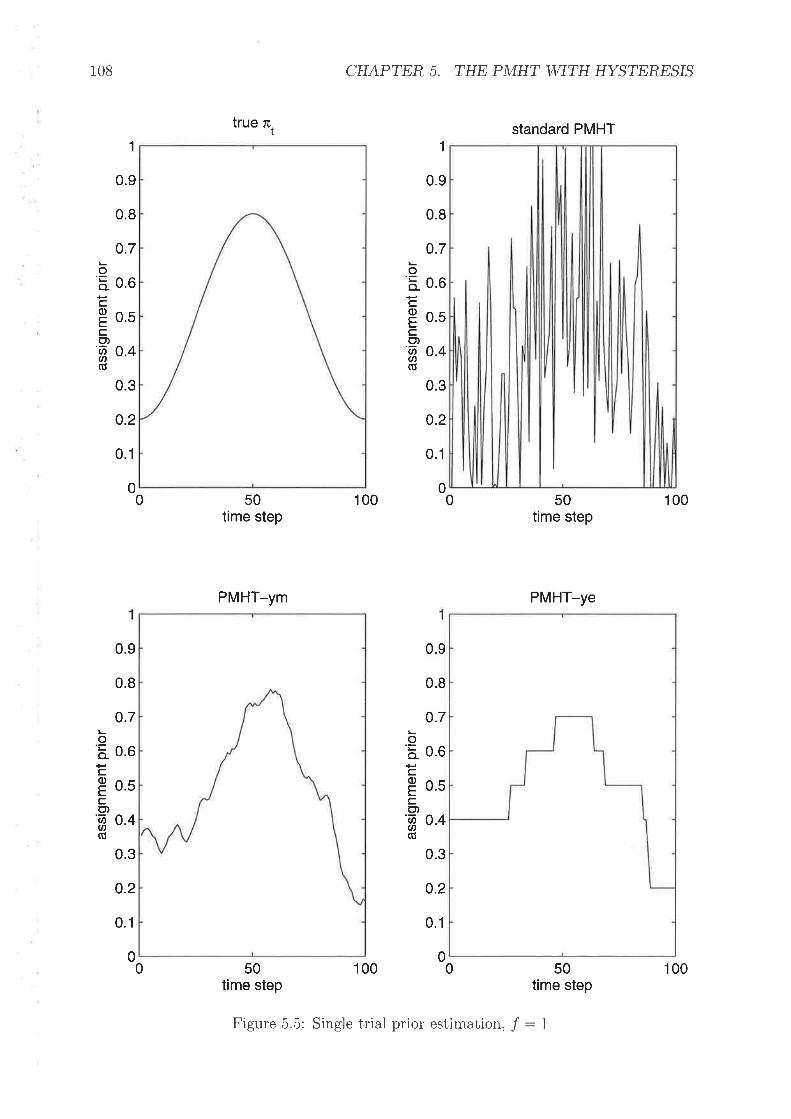
108 CHAPTER 5. THE PMHT WITH HYSTERESIS
standard PMHT1
true rc,
50time step
PMHT-ym
50time step
1
0.9
0.8
100
100
0.9
0.8
0.1
0.9
0.8
0.2
0.1
0.70.7Lo'ã 0.6C
Ê ost-C')
n 0.4(ú
0.3
õ'ã 0.6PcË o.sc(')g 0.4(ú
0.3
0.2o.2
0.1
0
0.9
0.8
000
0.70.7
0.60.6
0.50.5
0.40.4
0.30.3
0
50time step
PMHT-ye
50time step
100
L.oLo-LoEI_.9at)at)(ú
.oLo_coEc.9U)U)(ú
o.2
0.1
0 00
Figure 5.5: Single trial prior estimation, Í : I
100

5.7, SIMULATED EXAMPLE
Þoà_o(ú
oo_
1
2
J
4
5
6
7
B
I
10
11
10 20 30 40 50 60time step
70 80 90 100
Figure 5.6: PMHT-ym prior probability mass
1000 Monte Carlo realisations. The bias of each of the filters is shown in figure 5.7 andthe variance in figure 5.8.
The bias of the PMHT-ym is marginally better than the standard PMHT, and thatof the PMHT-ye is marginally worse. There is no significant difference between the threealgorithms in bias. However, the reduction in variance by using the assignment statemodel is dramatic. Both the PMHT-ym and PMHT-ye reduce the variance by an order ofmagnitude over the standard PMHT. This result is clear from the single realisation shownin figure 5.5. The high variance of the PMHT is clearly seen in the erratic variability notedearlier. The high variance of the standard PMHT is also seen by the variability in thebias curve in figure 5.7. This curve is averaged over 1000 trials, and the variance of theaverage is still apparent in the figure.
The variance of the PMHT estimate can be clearly seen to peak when the true prioris 0.5 and to have minima when it reaches the most one-sided points (nl : 0.2 andn¿1 :0.8). This is because the filter is estimating a binornial process, and the varianceof that estimate is expected to follow a r! (I - "l) curve analogous to that derived insection 4.4.2.
One reason for the dramatic reduction in variance is that the dynamics of the assign-ment state model allows the filter to effectivel)r use measurements from adjacent scans toestimate the prior for any particular scan. This is made quite obvious from the expressionmaximised by the HMM smoother, i.e. P (DrlX, Z). This is the probability of assignmentstate at scan ú given measurements over the whole batch. The effect of measurements fromdifferent scans is reduced the farther that scan is in time, depending on the diffuseness ofthe transition matrix, LT (dfldSr). fne standard PMHT uses neasurements only fromone scan) since it assumes that the prior at other scans is independent.
109

110 CHAPTER 5, THE PMHT WITH ¡TYS?ERESIS
tsoo(úEød)
.trat(dõ
0.15
0.1
0.05
0.12
0.1
0.02
0
-0.05
-0.1
-0.15
-H- 0.08Eo(dE
E o.oo'õo(ú.E
9 o.o+
10 20 30 40
010203040
Figure 5.7: Bias of estimator î1, f :1
60 70 80 90 100
60 70 80 90 100
50time step
50time step
0
PM-
PMHT' PMHT-ym
- PMHT
- PMHT-ym
Figure 5.8: Variance of estimator î|, Í : I

5.8. SUMMARY 111
5.7.3.2 Higher FÏequency Prior Variation
The sarne bias and variance curves are generated for a higher frequency variation in rl,with / : 4. The estimates from a single trial are shown in figure 5.9. In this case both thePMHT-ym and PMHT-ye appear to underestimate the true variation in the prior. Thetwo curves clearly vary at the same frequency as the true prior, but the departure frornrT :0.5 is reduced. This is actually a manifestation of the low-pass filtering propertyof the transition matrix chosen for the assignment state model. The variation in tltisexarnple is at a rate that shows significant attenuation by the filter, but not high enoughto be suppressed fully. This is also seen in the bias curve in figure 5.10. However, infigure 5.11, the variance of the PMHT-ym and PMHT-ye estimates remains an order ofmagnitude below that of the standard PMHT.
5.8 SummaryThis chapter introduced a dynamic model for the assignment prior probability. Thismodel is referred to as þsteresis. The hysteresis model uses an independent discretestate variable for each target model, so the assignment process is modelled with a Mxdimensional randomly evolving hyperparameter. Two alternative approaches for solvingthe generalised problem posed by the introduction of this model were considered: firstly,the state value was treated as missing data in an EM sense, and secondly, the state wasestimated.
The PMHT algorithm derived by treating the assignment state as missing data isreferred to as the PMHT-ym. The PMHT-ym determines the probability of the assign-ment state, in much the same way as the standard PMHT determines the probabilityof the assignments. This probability can be calculated using the Hidden Markov ModelSmoother.
The PMHT algorithm derived by estimating the assignment state values is referredto as the PMHT-ye. The PMHT-ye treats the assignment state in the same way as themodel states: an initial value is assumed, and then the algorithm iteratively updatesthe assignment state estimate based on the measurements. The refined assignment statesequence can be determined using the Viterbi algorithm.
The PMHT-ym and PMHT-ye were run on a simple sirnulated example to demonstratethe effect each has on the estimated assignment prior. The algorithms were run onmixtures with low and high frequency variation in their mixing proportions. It was foundthat by assuming a certain degree of smoothness in the hysteresis model, a low pass
filtering effect was achieved. The PMHT-ym and PMHT-ye both apply a restriction onthe rate of change of the prior, based on the assumed hysteresis model, which suppresseshigher frequency variations. Both algorithms dramatically reduce the variance over thestandard PMHT which assumes that the assignment prior is time independent. Thisreduction in variance is achieved because data from adjacent scans contributes to theprior estimate through the assumed dynamic model.

r72 CHAPTER 5. THE PMHT WITH HYSTERESIS
standard PMHT
0.9
0.8
o.2
0.1
100 50time step
100
PMHT-ye
0.8
100 0 50time step
1
true æ,
50time step
PMHT-ym
50time step
1
0.9
0.8
Loo_
coEco)ahat)(ú
.5
.4
.3
0
0
0
0.7
0.1
0
0.9
0.8
0.7
0.6
0.2
1
0.6
0.5
.40
0.3
0.7Lo'å 0.6cO nrE U'Ct-o)n 0.4(ú
0.3
000
1
0.9
Loo-coEc.9)|J,(t,(ú
0.7Lo'å 0.6cÊ o.sco)g 0.4(ú
0.3
0.2
0.1
0.2
0.1
00
0
Figure 5.9: Single trial prior estimation, Í : 4
100
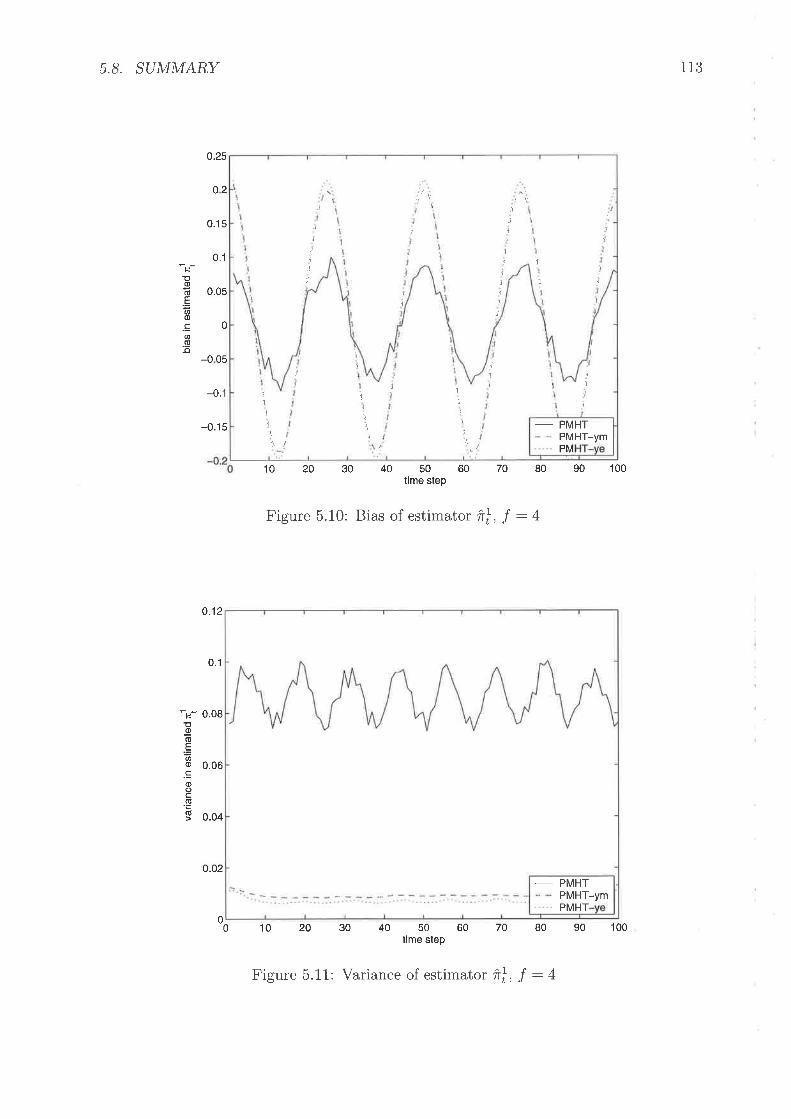
5.8. SUMMARY
o.25
0.15
0.1
0.05
-0.1
-0.15
0.12
0.1
o.o2
o2
0
HÞo)(úEØc)
.gah(d-o
-0 05
-H* 0.08Þo(úE.J)o 0.06.go()(ú.E
I o.o+
10 20 30 40
010203040
Figure 5.10: Bias of estimator î1, f : 4
60 70 80 90 100
60 70 B0 90 100
50time step
50time step
0
113
PM-
PMHT- PMHT-ym
j iiil
I
I
i¡
lIl
ì¡
I
I1
1
ì\
:\
'l'l
'I
J
!'|
J
l
1
J
1
I
II
PMHT-
PMHTPMHT-ym
Figure 5.11: Variance of estimator î.1, Í :4

tt4 CHAPTER 5. THE PMHT WITH HYSTERESIS

Chapter 6
Track Initiation and Initialisationwith the ProbabilisticMulti-Hypothesis Tracker
f-T-'tHE original Probabilistic Multi-Hypothesis Tracker derived by Streit and LuginbuhlI makes the assumption that the number of models is fixed and known. Further, it
assumes that the tracker has availabie a prior distribution for the state of each of thesemodels. In a realistic tracking situation, targets enter and leave the field of view of thesensor for various reasons. This means that the number of models that the tracker shoulduse (namely the number of targets in the scene) is an unknown and dynamic quantity.Since new targets appear inside the sensor field of view at unkuown locations, no priordistribution of their state is known, so a prior must be assumed based on sensor data.
In order to use the PMHT algorithm in an online implementation, it is necessary todevelop a method of initiating new tracks and terminating old tracks as new data arrives.This function may be performed manually by the sensor operator, however this may betime consuming and manual track management is only used if automatic management isunavailable or unreliable . It is desirable for the tracking algorithrn to be able to auto-matically perform the tasks of initiation and termination without operator intervention.
In addition to track initiation, the tracker rnust also be able to perform self initiali-sation. Namely the tracker should choose the initial state estimate automatically. ThePMHT is a numerical optimisation approach that iteratively converges to the MaximumLikelihood state estimate. However, it converges only to local maxima, and the initial-isation of the algorithm is therefore critical. Since the algorithm is required to initiatenew tracks, it must provide a method for initialising the state estimates of these tracks.The problem of poor initialisation is similar to the situation where a target manoeuvresand the previously accurate state estimate becomes biassed. Thus, incorporation of anautomatic initialisation scheme is anticipated to also improve tracking of manoeuveringtargets.
This chapter presents methods for addressing track initiation and initialisation withthe PMHT. Firstly, an initialisation technique is introduced which is based on the ho-mothetic measurement model of [RWS95a]. This method uses the innovation covariancematrix as a second measurement model. Since the innovation covariance matrix repre-sents the current uncertainty in the predicted measurement location, this method enablesthe PMHT to use a broad secondary measurement model when initialisation is poor, andto narrow this secondary model when good initialisation is obtained.
115
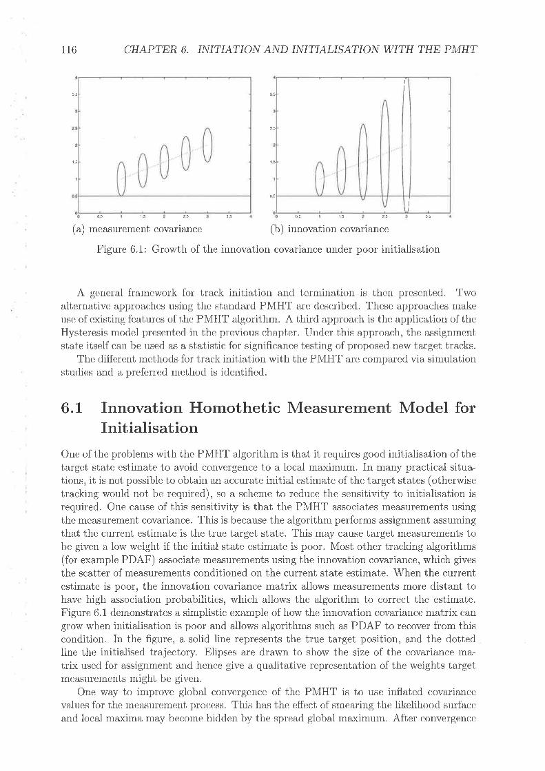
116 CHAPTER 6. INITIATIO¡\T A¡úD INITIALISATION WITH THE PMHT
35 35
25
1515
05
35
(a) measurement covariance (b) innovation covariance
Figure 6.1: Growth of the innovation covariance under poor initialisation
A general framework for track initiation and termination is then presented. Twoalternative approaches using the standard PMHT are described. These approaches makeuse of existing features of the PMHT algorithm. A third approach is the application of theHysteresis model presented in the previous chapter. Under this approach, the assignmentstate itself can be used as a statistic for significance testing of proposed new target tracks.
The different methods for track initiation with the PMHT are compared via simulationstudies and a preferred method is identified.
6.1 Innovation Homothetic Measurement Model forInitialisation
One of the problems with the PMHT algorithm is that it requires good initialisation of thetarget state estirnate to avoid convergence to a local maximum. In many practical situa-tions, it is not possible to obtain an accurate initial estimate of the target states (otherwisetracking would not be required), so a scheme to reduce the sensitivity to initialisation isrequired. One cause of this sensitivity is that the PMHT associates measurements usingthe measurement covariance. This is because the algorithm performs assignment assumingthat the current estimate is the true target state. This may cause target measurements tobe given a low weight if the initial state estimate is poor. Most other tracking algorithms(for example PDAF) associate measurements using the innovation covariance, which givesthe scatter of measurements conditioned on the current state estimate. When the currentestimate is poor, the innovation covariance matrix allows measurements more distant tohave high association probabilities, which allows the algorithm to correct the estimate,Figure 6.1 demonstrates a simplistic example of how the innovation covariance matrix cangrow when initialisation is poor and allows algorithms such as PDAF to recover from thiscondition. In the figure, a solid line represents the true target position, and the dottedIine the initialised trajectory. Elipses are drawn to show the size of the covariance ma-trix used for assignment and hence give a qualitative representation of the weights targetmeasurements might be given.
One way to improve global convergence of the PMHT is to use inflated covariancevalues for the measurement process. This has the effect of smearing the likelihood surfaceand local maxirna may become hidden by the spread global maximum. After convergence
05 15 35 05 15 25

6.1. I¡\I¡,TOVATION HOMOTHETIC MODEL rt7
with the inflated tneasurerlent covariance, the covariance is reduced somewhat and thealgorithm run again. This process is repeated until the final iteration where the truemeasuïement covariance rnatrix is used. This rnethod requires a choice of how much toinflate the measurernent covariance matrix and how quickly to approach the true value.Since the batch of data is processed several times, use of covariance inflation incurs asignificant computation cost.
To reduce the extra computational load required by covariance inflation, the degreeof inflation can be made adaptive. One way of adapting the inflated covariance is to usethe innovation covariance associated with the current state estimate. This allows highercovariance inflation for tracks with greater uncertainty.
The covariance inflation approach can also be automated by using the homotheticmeasurement model proposed in [Rl,VS95a]. Under the homothetic measurement model,the measurement process for each target is itself a mixture of Gaussians. Usually the mix-ture is composed of Gaussians that share a common mean, although this is not required.The homothetic measurement model can be used as a method of covariance inflation bymaking the measurement process a mixture of a Gaussian with covariance defined by theassumed "true" measurement covariance and a second Gaussian with covariance given bythe innovation covariance of the current state estimate. When the track estimate is firstinitialised, it is assìgned a high degree of uncertainty and the innovation covariance is high.As the trM iterations are performed, the smoothed state estimate gains higher accuracyand the innovation covariance is reduced. When the smoothed state estirnates are suffi-ciently close to the observed measurements, the algorithm associates the measurementswith the tighter density that uses the "true" measurement variance.
Figure 6.2 demonstrates how this approach allows the PMHT to recover from poorinitialisation through a mechanism similar to the PDAF shown in figure 6.1. The figureshows a sequence of plots. In each plot, false detections are shown with the symbol 'x'and valid detections '-l'. The estimated trajectory for that iteration of the PMHT isdrawn with a solid line, and elipses are drawn to show the innovation covariance. Asthe state estimate improves, the elipses shrink, indicating the the innovation covariancematrix corresponds to a tighter measurement scatter.
The standard homothetic measurement model for PMHT uses measurement covariancematrices which are scalar multiples of the true measurement covariance. This results instate estimation with the Kalman Smoother where the measurement covariance is replacedby a scalar multiple of the true measurement variance. The assignment weights determinethe scaling factor. The smoother uses a synthetic measurement which is a weighted sumof the sensor observations. As presented in chapter 3, these are given by
P:{
-r nt P:lnz¡ ttnt
r:1 p:l
wmptr
KÌNP t t umptrKrnp
(6 1)
(6 2)
Zb¡r:I P:1'
and-1
Rr \- \- untqtrL L pimq
RrntP
r:7 p:1
where n^p is the scalar multiplier for the measurement variance associated with homoth-etic model p and umptr is the assignment weight for model p of fiack m.
The results in (6.1) and (6.2) do not hold when the second model is the innova-tion matrix because the innovation covariance is not necessarily a scalar multiple of the

118 CHAPTER 6. INITIATIO¡\T A¡\ID INITIALISATIO¡\I WITH THE PMHT
initialisation
X\
iteration 1 iterat¡on 2\70
EI
70 x 70
6565 XX
x
zXI
X
ñXX
x
I
XX55
50
x
50
Xu
\þ:
xX
xX
rntnt(nf) ^ : t uJmttu(Rf)-' + t um2tr(Sf)-',
65
cE'B 60o.
c.9'8 60o-
JX .9'8 60o- 6'X x X
IXv.
X\
X
-25 -20 -15 -10x position
55 \%X\
X
X X
-25 -20 -15 -10x position
iteration 3I
-5 -5 -20 -15 -10x position
-5
-20 -15 -10 -5x position
-20 -15 -10 -5x position
iteration 5
xt,.
-20 -15 -10x position
¡teration 4X70
65
x
c.o'8 60o-
x,¿
\
x
70
65++^d
70
65
60
c.9'8 60o.
o'õoo
X7.X
5555
X
XxX 55 XLx X
X X
-5
Figure 6.2: Correction for poor initialisation with innovation homothetic model
measurement variance. However, the state estimate can stiil be solved using a KalmanSmoother. The smoother uses a synthetic measurement and covariance defined by
arrL.t n¡ l,lr-rr, (Rf)-t Iu^2t (sT)-tl "*nt
(6 3)r:1
and
(6 4)r:1 r:L
where Si" is the innovation covariance matrix for model rn at scan Í.The expressions (6.3) and (6.4) are more generalised versions of those in (6.1) and
(6.2) respectively. They sirnplify to the latter expressions if the matrix Sfl can be writtenas rcRf, with rc constant. The derivation of (6.3) and (6.a) is presented, along with amore detailed discussion of this generalised homothetic model in Appendix A.
6.2 Initiation MethodologyThe process of creating new tracks when new targets are detected is called track initia-tion, or track formation. There are numerous techniques for solving the track initiationproblem, but each of them can be formulated under a common framework of candidate

New candidates Residualmeasurements measufements
Established tracktest
Candidate tracks Track updateassociation/estimation
Track updateassociation/estimation
Retain RetainEstablished tracksCandidate
quality test
6,2, INITIATION METHODOLOGY 119
Dclete
Candidate Tracker Delete : Established Tracker
Figure 6.3: General initiation flow diagram
tracking. Using the radar measurements, candidate tracks are initialised at possible targetlocations. Candidate tracks might be started on all measurements, or on a subset, ac-cording to a selection rule. For example, one might choose measurements not assigned toan existing target model which are sufficiently close to a measurement from the previousscan. However formed, the candidate tracks are allorved to assign measurements and areupdated. After a number of scans, the candidates are tested using a decision rule. Basedon this test, candidates may be discarded or promoted to established tracks. The decisionto promote or discard may be deferred, and the candidate retained.
Figure 6.3 shows a typical scheme for tracking with automatic initiation. In figure 6.3established tracks, which were initiated at some earlier time, get the first pickings of thesensor measurements. These tracks remove measurements that have a high assignmentprobability and the remaining measurements (the residual measurements) are used toform candidate tracks. The candidate tracks perform association and state estimationusing the residual measurements. This prevents the candidate tracker from running acandidate track on the same target as is represented by an established track.
A possible fault with the scheme shown in figure 6.3 is that the association of measure-ments and the updating of state estimates should perhaps be done jointly for all tracksrather than in the sequential manner shown. A scheme performing this joint associationand update is shown in figure 6.4. The danger with the sequential approach is that anestablished track will be assigned measurements from more than one target and it willprevent new tracks forming on the other targets. This is likely to occur with the jointscheme anyway since the new candidates must be formed from the residual measurements)otherwise multiple tracks will be formed on every target.
A danger with the joint scheme is that candidate tracks will degrade the establishedtracks. Suppose there is a track following a target that performs a heading change. Theestablished track may take a few scans to adjust heading to the new trajectory, In themeantime, a candidate track has been started on the new heading and is very close tothe measurements since they were used to initialise it. The candidate track is assignedthe measurements in preference to the established track since the established track isfarther from the correct state estimate. The consequence is that the established trackwill be terminated and the new candidate track will be promoted. This is undesirableperformance which is easily prevented by using the sequential approach.
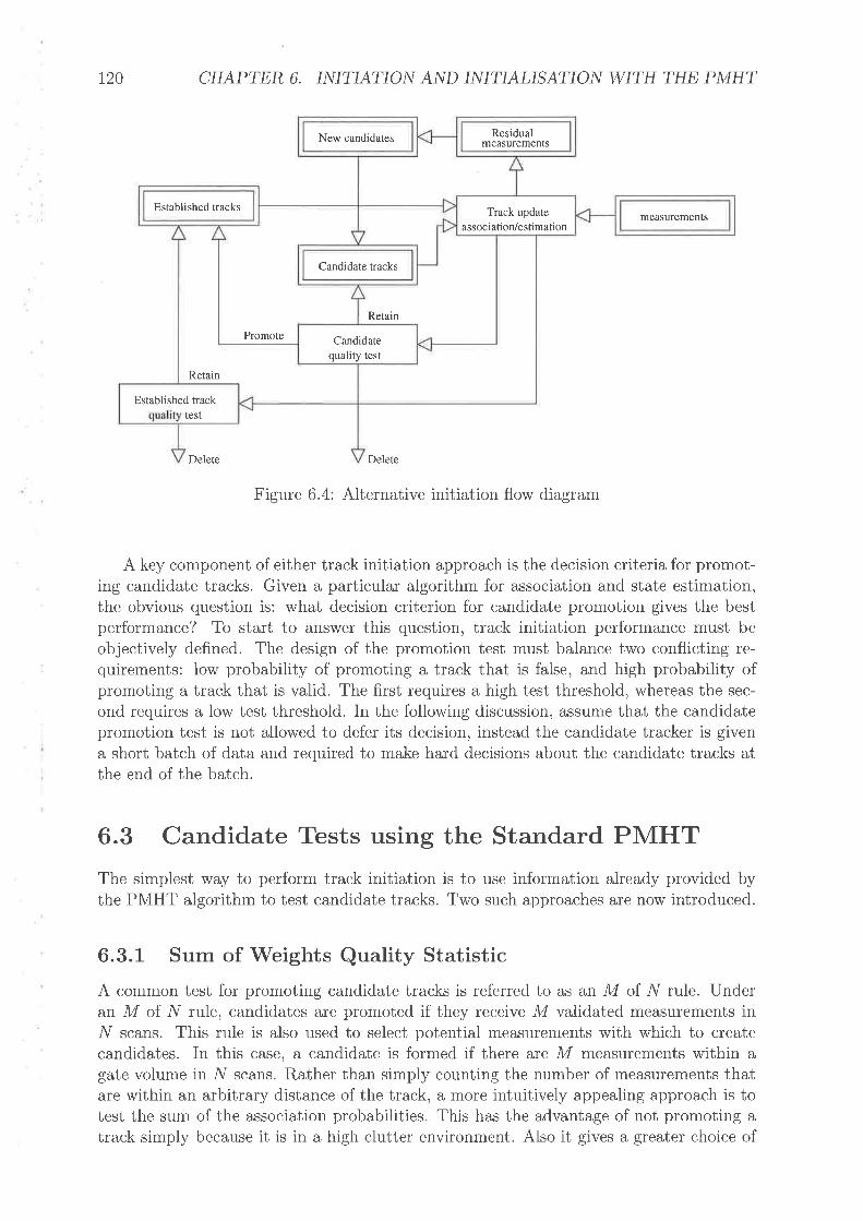
New candidates Residualmeasufements
Established tracks Track updateassociation/estimation
measurements
Candidate tracks
Promote
Retain
Candidatequality test
Retain
Established tracktest
L20 CHAPTER 6. INITIATIO¡\T A¡\TD INITIALISATION WITH THE PMHT
Delete Delete
Figure 6.4: Alternative initiation flow diagram
A key component of either track initiation approach is the decision criteria for promot-ing candidate tracks. Given a particular algorithm for association and state estimation,the obvious question is: what decision criterion for candidate promotion gives the bestpedormance? To start to answer this question, track initiation performance must beobjectively defined. The design of the promotion test must balance two conflicting re-quirements: low probability of promoting a track that is false, and high probability ofpromoting a track that is valid. The first requires a high test threshold, whereas the sec-ond requires a low test threshold. In the following discussion, assume that the candidatepromotion test is not allowed to defer its decision, instead the candidate tracker is givena short batch of data and required to rnake hard decisions about the candidate tracks atthe end of the batch.
6.3 Candidate Tests using the Standard PMHTThe simplest way to perform track initiation is to use information already provided bythe PMHT algorithm to test candidate tracks. Two such approaches are no\¡/ introduced.
6.3.1 Sum of Weights Quality StatisticA common test for promoting candidate tracks is referred to as an M of.l/ rule. Underan M of Iy' rule, candidates are promoted if they receive M validated measurements inly' scans. This rule is also used to select potential measurements with which to createcandidates. In this case, a candidate is formed if there are M measurements within agate volume in l/ scans. Rather than simply counting the number of measurements thatare within an arbitrary distance of the track, a more intuitively appealing approach is totest the sum of the association probabilities. This has the advantage of not promoting atrack simplv because it is in a high clutter environment. AIso it gives a greater choice of

6.3, CANDIDATE TESTS USIAIG THE STA¡úDARD PMHT I2t
promotion threshold, since the test statistic is no longer integer valued. This leads to asimple ad hoc quality statistic given by the sum of the association weights:
Tntqi:ttumtr' (6.5)
t:7 r:1
This statistic can be interpreted as the estimated number of measurements caused bymodel rn. When normalised by the total number of measurements in the batch, qT rs
also the maximum likelihood estimator for the prior probability of a measurement beingcaused by model rn if this prior is time invariant.
This simple quality statistic will be referred to as the sum of wei,ghts quality statistic(for obvious reasons) and is used as a benchmark for other proposed initiation schemes.The sum of weights test could be implemented with no alteration to the PMHT algorithmand carries very little overheads.
6.3.2 Cost Function IncrementAnother commonly used quality test for candidate tracks is the cumulative log likelihoodof the assigned measurement sequence [Sit64]. The log likelihood can be determined byaccumulating the squared innovations when the statistics are assumed to be Gaussian,i.e.
rnlTrltq"" : -,t t w^r,(HyFT*7, - tr,)'(sf)-t (nyr7æ7r - ztu) (6 6)I L:t ,:r
Intuitively, false tracks are expected to be assigned measurements that match thetarget dynamic model poorly and have a large scatter about the predicted measurements.Such tracks will have a high accumulated innovation and this can be used to reject them.This statistic gives a measure of how well the measurements assigned to a track fit theassumed target model.
An analogue of this approach for the PMHT would be to use the component of theauxiliary function corresponding to that model as the quality statistic, namely
ATT
'IT¿q
roe,þL @T) +I to*,þ7 @Tl*7,) * D f tos (í" ("Í:'Wf) umtr. (6 z)Tnt
t:7 r:lt:1.
Note that an iteration index is not included on the weights because the quality statisticis only calculated on convergence of the algorithm.
There are two main problems with this approach. Firstly, a track with very fewrneasurements assigned to it will clearly not have very high measurement scatter and so
be treated as a good candidate track. Such tracks are not good candidates; the lackof assigned measurements is a strong indicator that the track is only assigned cluttermeasurements. To deal with this case, the log likelihood test must be augmented with aIogical test to require the candidate to assign a certain number of measurements.
The second problem is that the test is centred on the track itself. The goal of addinga new track is not to add a new model which assigns measutements. Rather it is toadd a model which accounts for measurements which seem unlikely under the currentmixture model. To this end, the test statistic should encompass the overall improvementin the data description by the inclusion of a new model. This point is best illustrated

t22 CHAPTER 6. INITIATIO¡\T A¡\ID INITIALISATIOAT WITH THE PMHT
with an exarnple. Suppose there is a sequence of valid target measurements. A targetmodel on these measurements will give a good quality statistic. Further suppose that atarget model assigns most of these measurements, but that a candidate track is initialisedon them anyway. The candidate will be given significant weights for the measurements,and the weights for the pre-existing track will be reduced. Depending on the promotionthreshold, this new candidate may be promoted even though it adds nothing to the overalldescription of the data.
Both of the above problems can be addressed by using the total system likelihood as
the quality statistic, rather than the individual model likelihood. Under this approach, thequality assigned to a new candidate is the improvement in the overall likelihood obtainedby adding the candidate. This improvement is given by
qa:Q(x,x") -a(x) , (6.s)
where X" is the candidate state sequence and X are the states of the other models.The addition of the candidate model is guaranteed to increase the auxiliary function,
and the amount of this increase provides a measure of how much the candidate modeladds to the overall data description. This approach was used to estimate the numberof components and the parameters of a Gaussian mixture with an unknown number ofcomponents by Vlasis et al. in [VLK00, VL00].
6.3.2.I Comparison with Model Order Estimation
The track initiation problem is really one of model order estimation. The aim is to find thebest set of dynamic Gaussian models to describe the sensor data. The solution requiresboth the determination of the states of each component and an estimation of how manycomponents provides the best fit to the data. This latter part is model order estimation.
It is not possible to use standard optimisation approaches for model order estimation.Optimisation criteria such as Maximum Likelihood or Least Squared Error will alwaysprefer a model of higher order. Ultimately, such methods will find the optimal model orderto be any number at least as large as the number of data points. Once the number ofparameters is more than the number of data points, adding further complexity producesno change in the optimising objective function. To alleviate this shortcoming, model orderestimation approaches incorporate a penalty term which reduces the objective functionwhen a higher order rnodel is used. This penalised objective function is then of the form
A(X) : IoB L (x,4 - f @6), ¡/), (6 e)
where d is the total number of parameters (the sum of the lengths of all the state vectors)and lú is the total number of data points, namely l/ : D, nt. L is the maxirnum valueof the likelihood of the data under model X, i.e. the likelihood when X is set to the MLestimate, The model order is then that integer d which maximises the function Ç.
The A Informat'ion Cri,teri,on (AIC) was developed by Akaike [Aka7a] by minimisingthe Kullback-Leibler distance between the true data model and the estirnated model. Thederivation of the AIC relies on asymptotic arguments. The AIC is given by
Qo,r: log I (X, Z) - 2d(X). (6.10)
A problem with the AIC is that the penalty term is independent of the size of the dataand so the model order will be overestimated when l/ is large. Both Schwartz [Sch78]and Rissanen [Ris78] are critical of the arguments used to derive the AIC.
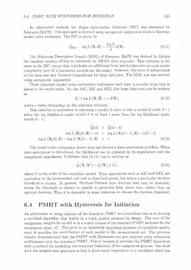
6.4. PMHT WITH HYSTERESIS F'OR INITIATION t23
An alternative method, the Bayes Informati,on Criteriorz (BIC) was presented bySchwartz [Sch78]. This approach is derived using asymptotic argutnents about a Bayesianmodel order technique, The BIC is given by
Q",, :log I (x, z) - los^N d(x) (6.11)t/2
The Minimum Description Length (MDL) of Rissanen [R,is78] was derived by findingthe smallest number of bits to represent an ARMA data sequence. This criterion is thesame as the BIC except that it includes an additional term which takes into account modelcomplexity (not all d parameter models are the same). However, this term is independentof the data size and becomes insignificant for large data sets. The MDL was also derivedusing asymptotic arguments.
These standard model order estimation techniques each have a penalty term that islinear in the model order. So, the AIC, BIC and MDL (for large data sets) can be writtenAS
Õ : loe ¿ (X, Z) - , d(x), (6.12)
where e varies depending on the selection criterion.This criterion is equivalent to choosing a model of order d over a model of order d - 1
when the log likelihood under model d is at least e more than the log likelihood undermodel d - l:
a@) >log l (x(d),2) - ed >
log I (X(d),2) - log I (X(d - r),2) >
The model order estimation above does not involve a data association problem. Whendata association is introduced, the likelihood can be replaced by its expectation over theassignment hypotheses. It follows that (6.13) can be written as
Q(X,X") -A(X) ) Ce, (6.14)
where C is the order of the candidate model. Thus, approaches such as AIC and MDL areequivalent to the incremental cost test as described above, but where a particular decisionthreshold is chosen. In general, Neyman-Pearson type detector laws may be desirable,where the threshold is chosen to specify a particular false alarm rate, rather than anoptimal decision. Thus it is desirable in some instances to choose the decision threshold.
6.4 PMHT \ /ith Hysteresis for InitiationAn alternative to using outputs of the standard PMHT as a candidate test is to developa modified algorithm that builds in a track quality measure by design. The sum of theassignment weights for model m is a scaled version of the standard PMHT estimate for theassignment prior, ri. The prior is an intuitively appealing measure of candidate qualitysince it specifles the contribution of each model to the measurement set. The previouschapter demonstrated that the PMHT with Hysteresis can give superior prior estimationperformance over the standard PMHT. This is because it provides the PMHT frameworkwith a method for modelling the temporal behaviour of the assignment process. One faultwith the weights sum approach is that it gives equal importance to a candidate which has

L24 CHAPTER 6. INITIATION AND INITIALISATION WITH THE PMHT
two assigned measurements in one scan, and a candidate which assigns one measurementper scan in two consecutive scans. It is evident that the latter is more likely to be a validtrack. When the Hysteresis nodel is used, the Markov chain of the assignment processcan be designed so that the assignment state itself is an in-built quality measure of thecandidate.
When a candidate track is valid, then it is detected with probability Pd and if it isdetected, then it forms one measurement. Thus, the true ri of a valid candidate i" #.If the candidate is false, then the true rl is zero. An obvious quality test for candidatesis thus the estirnated ri value. This is the weights sum approach already discussed.However, the estimated ri has a high variance) as demonstrated in the previous chapter.This then motivates the use of the PMHT-y model for smoothing the rfl estimate, andwas actuallv the problem which inspired its development.
6.4.L Initiation \Mith PMHT-ymThere are two types of candidate tracks: valid and false. Since this analysis assurnes afixed probability of detection Pd, which is the same for all targets, then there are two truevalues of rf, as stated above. An intuitive decision is thus to use an assignment statespace with two possible state values corresponding to false and valid tracks, i.e. Mp : ).This is the simplest possible model, and has the benefit of minimising the computationalrequirements of the algorithm. Under this model,
óT@ :óT0 : (6.15)
This special case, with a binary assignment state model, is the same as the visibilitymodel used for initiation with the PDAF and other filters. Section 5.2.1 discusses therelationship between the visibility approach and the hysteresis assignment model. Forthis special case, the assignment state for model m, dT, will be referred to as the visibilityof model m and the PIVIHT-ym using this model is referred to as the PMHT with visibility,or PMHT-v.
The PMHT-v calculates the posterior probability mass P (dT :1), which is the prob-ability that the candidate has a prior consistent with a valid track. This then providesa natural quality statistic. Since the visibility variable can change over the batch, thecandidate test statistic is
rn 7Tni : Tf r @,7 : rlx,z). (6.16)t:l
All that remains is the seiection of the transition probability matrix and the priorprobability mass. Since the model is binary (Mo :2) these are fully specified by threeparameters: Aff (dff) has two elements, one of which is constrained by normalisation, andLT (d,Tl¿\r) has four elements, two of which are constrained by normalisation. Theseparameters are design parameters which can be chosen either by subjective belief, or byoptimising particular criteria.
In [LL01b] a set of heuristic rules is optimised in order to select parameters of theperce'iuabzli,ty modeL This model is visibility by another name (in the PDAF context of[CDA86]), and [LL01b] is the only work to address the issue of parameter selection. Otherauthors either present quantities with no explanation, or do not provide these numbers
0,
PdTù¡

6.4, PMHT WITH HYSTERESIS FOR INITIATION 725
due to propriety issues. The parameters derived in [LL01b] are
P (di : r) : 0.5,
P (d,T : Tld2t: r) : 0.988,
P (d,T : rldir: s) : o.o.
The method used for initiation performance analysis used in this thesis is the initiationReceiver Operating Characteristic curve (described in detail in section 6.5.1). So, it issensible to optimise the parameters for the curve. This confirmed the above parameters,with the exception of the prior probability, which was instead chosen as
P (dT : 1) : 0'1'
6.4.L.I The PMHT-v algorithm
In the analysis to follow, the special form of the PMHT-ym used for track initiationis referred to as the PMHT-v. This is because the algorithm is the PMHT version ofthe visibility based initiation approach particularly popular with PDA. Unlike the PDAinitiation algorithms the PMHT version of visibility has a solid theoretical foundation;various authors make claims about the superiority of their PDA models based mainly onthe interpretation of the model. The interpretation of the Hysteresis model is clear andfits easily into the PMHT framework.
For completeness, a summary of the PMHT-v is now presented. Notice that the setD¿ is now a binary vector, and thus Dr. D, gives the number of elements in D¿ whichare unity. The PMHT-v proceeds as follows:
1. Initialise the estimates X(0) and X(0).
2. Determine the posterior probability of assignment state using
P (Dlxu-t),2) : at(Dr) þ'(Dr)Ðu a'(Dt : U) 0' (D, : u)
where at(Dt) and B¡(D¿) are defined using (5.25) and (5.26)
ar(Dr): tMa
lI or (¿Tt¿T,) P (ZtlDt,Xr) ",-r (Dr_1) ,
Dt-t m:1.
MaP (Zr*rlDr*r,Xr+t) 1r+t(Dr*t1 ,
Dt+t m:l
and the incomplete conditional data likelihood P (ZlDüX¿) can be written as
lvlv
Ð"-ef Q"þT)
0, (Dr): t fl oïL' @'T*'ld'T)
Pd t d,T-*" er Q,,l*T)
P (2, D,,x,) : I { (t - 4o,, o') m:I
+A/Í
TL¡ rn:NIv*7
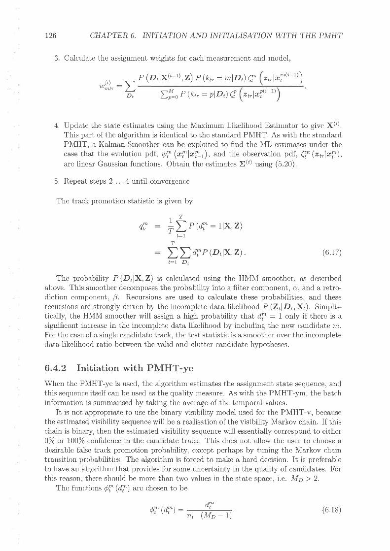
126 CHAPTER 6. INITIATIO¡\I A¡\ID INITIALISATIO¡\I WITH THE PMHT
3. Calculate the assignment weights for each measurement and model,
P (DIXQ-L),2) P (kr, : mlDr) Ç ztu@TQ-1))tDt Dy:, P (k* : plD') Ç
t n(i-l\zblæi'
4, Update the state estimates using the Maximum Likelihood Estimator to give [(l).This part of the algorithm is identical to the standard PMHT. As with the standardPMHT, a Kalman Smoother can be exploited to find the ML estimates under thecase that the evolution pdf, ,þT @Tl*7,), and the observation pdf, eT Q*lrT),are linear Gaussian functions. Obtain the estimates )(i) using (5.20).
5. Repeat steps 2 . . .4 until convergence
The track promotion statistic is given by
11.IU-¡,
qT1T;t P@,7:rlx,z)
t:7T
t t dTP (Dlx,z) . (6.17)t:t Dt
The probability P (D|){',Z) is calculated using the HMM smoother, as describedabove. This smoother decomposes the probability into a filter component, o, and a retro-diction component, p. Recursions are used to calculate these probabilities, and theserecursions are strongly driven by the incomplete data likelihood P (ZrlDr,X¿). Simplis-tically, the HMM smoother will assign a high probability fhaf di : 1 only if there is asignificant increase in the incomplete data likelihood by including the new candidate rn.For the case of a single candidate track, the test statistic is a smoother over the incompletedata likelihood ratio between the valid and clutter candidate hypotheses.
6.4.2 Initiation with PMHT-yeWhen the PMHT-ye is used, the algorithm estimates the assignment state sequence, andthis sequence itself can be used as the quality measure. As with the PMHT-ym, the batchinformation is summarised by taking the average of the temporal values.
It is not appropriate to use the binary visibility model used for the PMHT-v, becausethe estimated visibility sequence will be a realisation of the visibility Markov chain. If thischain is binary, then the estimated visibility sequence will essentially correspond to either0To or 100% confidence in the candidate track. This does not allow the user to choose adesirable false track promotion probability, except perhaps by tuning the Markov chaintransition probabilities. The algorithm is forced to make a hard decision. It is preferableto have an algorithm that provides for some uncertainty in the quality of candidates. Forthis reason, there should be more than two values in the state space , i.e. M ¡, ) 2.
The functions þi @i) are chosen to be
óT @ï\ : ,!T ,,. (6 1s)' n, (Mo - I)'

6.4. PMHT WITH HYSTERESIS FOR INITIATION r27
Thus, higher values of di correspond to models which contribute more measutementsto the mixture and are hence more likely to correspond to valid targets. M¡ is nowequivalent to a quantisation level of
"h in the óT @T) used for the PMHT-v in the
previous section.Heuristic specifications on the transition matrix are provided by intuition: the rnatrix
should be dominantly diagonal with the probability of switching between extrerne endsof the assignment state space being very low. When the main diagonal of the transitionmatrix is strongly dominant, then the estimated state sequence will smoothly transitionbetween values.
The transition matrix has Mo(Mo - 1) free elements to optimise. To sirnplify theparameter optimisation, it was chosen to limit the freedom of the transition matrix byassuming the following form:
^i @i)1
Mp Ym
LT @'T : jld\t:d) d,¿exp
(6.1e)
(6 20)
(6 21)
where op is now the only design parameter, and this quantity controls the dominance ofthe diagonal elements. d¿ is a normalising constant that ensures that all of the transitionsfrom state i sum to unity probability and is given by
,,:{M¡1tj:r /. '\t\L-J).
Mn-itexp2 (oDMD)2 l) j:L-¿
d¿ is the inverse of the sum of the exponential function in (6.20) over a window thatslides according to ¿. It will take its biggest value for i,:1 and i,: Mn. This means thatthe diagonal terms in the transition matrix are biggest for the extreme visibility values.The matrix defined by (6.20) and (6.21) is shown in figure 6.5 for a particular value ol op.The brightest areas show the greatest probabilities, and these areas are found near thetop left and bottom right end of the matrix. This tends to encourage the model towardsextreme values.
6.4.2.I Parameter Selection for the PMHT-yeThe above hysteresis model for initiation with the PMHT-ye still has two parametersto select: the dimension of the assignment state space, Mp, and the dominance of thetransition diagonal, controlled lry on. These could be chosen by subjective belief, orpreferably by optimisation of an objective criterion. As in section 6.4.1, the appropriatecriterion to use is the initiation Receiver Operating Characteristic (ROC) curve, since theROC will be used as the performance measure for track initiation. The ROC curve fortrack initiation is discussed in detail in section 6.5.1. The parameter Mo is chosen to beas small as possible, while maintaining high performance. The transition parameter, o¡is chosen to give the best ROC curve.
The PMHT-ye is not included in the initiation analysis which is to follow. This isbecause it was found to give poor performance. When the algorithm was able to recoverfrom initialisation and follow the target trajectory, it easily discriminated the valid targettrack from false tracks due to clutter. Howevet, on difficult realisations (usually whenthe target was not detected for several scans near the start of the batch) the PMHT-yefailed to recover from initialisation and diverged from the true trajectory. Essentially it

728 CHAPTER 6. INITIATIO¡\I A¡\ID INITALISATIO¡\T WITH THE PMHT
5
t 10 15 20 25 30 35 40 45 50
performed excellently on the simple cases, but very poorly on the more difficult casesFor this reason, it is not considered further.
6.5 Performance Analysis MethodSeveral methods for track initiation with PMHT have now been presented. These methodswill be compared in this chapter through simulation. However, the measures used inprevious chapters (such as the mean squared estimation accuracy) are not appropriatefor track initiation. Instead, the performance measure for track initiation should quantifyhow well the candidate test discriminates between valid and false candidate tracks. Thiswill be done by using a Receiver Operating Characteristic curve.
6.5.1 The Receiver Operating Characteristic CurveThe track promotion test in the initiation process is a decision and can be viewed asa detector. The promotion test aims to detect valid target tracks and to reject falsetracks that associate clutter measurements. One way of quantifying the performance of adetector is through the use of a Receiver Operating Characteristic curve. The ROC plotsthe probability of correctly detecting a desired signal as a function of the probabilityof incorrectly detecting a noise signal (a false alarm). Each point in the locus of thecurve represents a particular detector setting (threshold). The ROC curve summarisesthe probability of detection and the probability of false alarm for all possible detectorparameter choices and thus provides a measure of how well the test discriminates validand false signals.
Figure 6.6 shows an example ROC curve for track initiation. Whereas the standard
10
20
25
30
35
40
45
50
Figure 6.5: Transition matrix., L! (¿T : j dTt: ¿), for Mn : 51
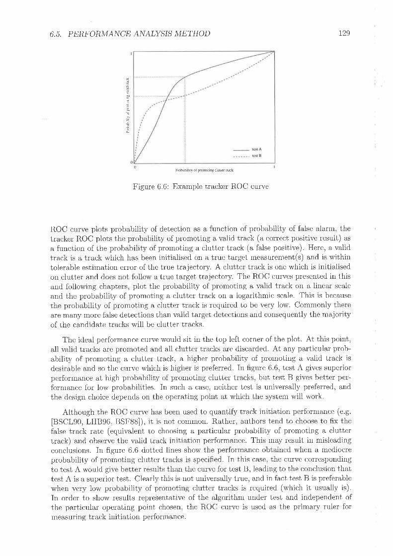
6.5. PERFORMA¡\ICE A¡\IALYSIS METHOD t29
q
E
-
0Probability ol promoting clutter lrack
Figure 6.6: Example tracker ROC curve
ROC curve plots probability of detection as a function of probability of false alarm, thetracker ROC plots the probability of promoting a valid track (a correct positive result) as
a function of the probability of prornoting a clutter track (a false positive). Here, a validtrack is a track which has been initialised on a true target measurement(s) and is withintolerable estimation error of the true trajectory. A clutter track is one which is initialisedon clutter and does not follow a true target trajectory. The ROC curves presented in thisand following chapters, plot the probability of promoting a valid track on a linear scaleand the probability of promoting a clutter track on a logarithmic scale. This is becausethe probabitity of promoting a clutter track is required to be very low. Commonly therea e many more false detections than valid target detections and consequently the majorityof the candidate tracks will be clutter tracks.
The ideal performance curve would sit in the top left corner of the plot. At this point,all valid tracks a e promoted and all clutter tracks are discarded. At any particular prob-ability of promoting a clutter track, a higher probability of promoting a valid track isdesirable and so the curve which is higher is preferred. In figure 6.6, test A gives superiorperformance at high probability of promoting clutter tracks, but test B gives better per-formance for low probabilities. In such a case, ueither test is universally preferred, andthe design choice depends on the operating point at which the system will work.
Although the ROC curve has been used to quantify track initiation performance (e.g.
[BSCL9O, LHB96, BSFSS]), it is not common. Rather, authors tend to choose to fix thefalse track rate (equivalent to choosing a particular probability of promoting a cluttertrack) and observe the valid track initiation performance. This may result in misleadingconclusions. In figure 6.6 dotted lines show the performance obtained when a mediocreprobability of promoting clutter tracks is specified. In this case, the curve correspondingto test A would give better results than the curve for test B, leading to the conclusion thattest A is a superior test. Clearly this is not universally true, and in fact test B is preferablewhen very low probability of promoting clutter tracks is required (which it usually is).In order to show results representative of the algorithm under test and independent ofthe particular operating point chosen, the ROC curve is used as the primary ruler formeasuring track initiation performance.

130 CHAPTER 6. INITIATIO¡\¡ A^ID INITIALISATIO¡\r WITH THE PMHT
6.5.2 Other Performance Assessment ApproachesThe ROC curve is a good method for assessing track initiation performance, but this isonly one facet of the tracking algorithm. Aspects such as manoeuvre handling, estimationerror) overshoot and false track duration are all important factors in overall tracker rating.In [CDD96], seventeen metrics for tracker performance are used to compare competingalgorithms. This approach is more appropriate to gain an overall indication of trackingperformance. However, he main focus of this thesis will be track initiation performancequantified via the ROC curve. Other studies have already considered the performanceof PMHT under established track criterion, such as estimation accuracy (for example,[RWS95a, R\\¡S99, RW01a, WRS98b]).
6.5.3 Generating ROC Curves Fþom Simulated DataIn section 6.5.1 the track initiation ROC curve was introduced as a method for evaluatingthe performance of track initiation schemes. This curve is the locus of the probability ofpromoting a track, given it is associated with a valid target, as a function of the probabilityof promoting a track, given it is false. The problem with using the ROC curve is that thesetwo promotion probabilities cannot be analytically derived for complicated algorithmssuch as the PMHT and its variants. This means that the true ROC curve cannot becomputed, and an approximated one must be used in its place. This approximated ROCcurve is produced by estimating the promotion probabilities above. These estimates areobtained using Monte Carlo simulation.
The true ROC curve is composed of the promotion probabilities which are the curnu-lative distributions of the qualitv statistic
P(promotelvalid;ú) : [* p(qlrutid)dq, (6.22)Jt
where ú is the promotion threshold. Given a sample of l/ valid tracks, this probabilitycan be approximated by
1åP(promotelvalid;ú) = i L,I (q" ¿t), (6.23)
n:l
where 1(') is an indicator function taking the value unity when its argument is true andzero when it is false. This is equivalent to approximating the density p(qlvalid) with asum of dirac delta functions, each shifted to the location of one of the observations
¡¿
p(qlvalid) = I6(q- q,). (6.24)n:l
Using the approximation in (6.23) may lead to a noisy estimated ROC curve. One wayto smooth the estimated ROC is to use a smoother density estimate for the promotionprobability. This may be done by using a kernel density approximation lSilS6]
p(qlvalid) =:Ë lr(q-q"\ , rc.25)N#''\ s /where the kernel function, 4, is a normalised, smooth. function. If the support of the kernelfunction is fixed at (say) [-1,1], then the dilation parameter, s, controls the support ofthe contribution of each observation, and hence the smoothness of the pdf estimate.

6.6. SIMULATED TRACK INITIATION P,trRFORMANCE 131
Using this kernel estimator, the smoothed estimated cumulative density function is
p(promotervarid;ú) = + ä1,-:r (1ø) ., rc'6)
The ROC curves that are presented in this thesis have all been generated using aquadratic kernel function
rt(q) : q2 - r, (6.27)
with a dilation parameter, s : 0.1.
6.6 Simulated Track Initiation PerformanceThe performance of three of th.e PMHT track initiation approaches presented in thischapter is now examined through simulation. These approaches are
1. The standard PMHT algorithm using the sum of the candidate assignment weightsas a promotion test statistic. This approach is referred to as the we'ights surn (see
section 6.3.1).
2. The standard PMHT algorithm using the incremental improvement in the EM auxil-iary function by introducing a candidate as a promotion test statistic. This approachis referred to as the cost'increment (see section 6.3.2).
3. The PMHT-ym algorithm using visibility for the assignment state model. Thecandidate promotion test statistic is the average probability that the assignmentstate is that of a visible target. This approach is referred to as PMHT-v (see
section 6.4.1).
A crucial factor in the production of the initiation ROC curves is a knowledge of theunderlying truth. The statistics are conditioned on knowledge of whether each track is
valid or false. In order to guarantee this knowledge, two test scenarios are used. Toestimate the candidate statistics of false tracks, a scene containing no target is used. Thestatistics of valid tracks are estimated using a scene with a single target, and a validtarget measurement is used to initialise the track. The valid candidate is discarded if thefinal state estimate deviates from the true target state by more than a prescribed amount.This approach avoids the possibility of coincident tracks, and false tracks being assignedvalid target measurements.
The simulated target model is the two dimensional almost constant velocity model(see section 3.3 for more details on the almost constant velocity target model). This is acartesian model, with target motion independent in the two coordinate axes.
The sensor provides a two dimensional measurement vector which contains an obser-vation of the target position in each dimension, corrupted with independent noise. Thisis a linear Caussian modcl. Diffcrent distributions of the clutter measurements are con-sidered, although each consists of only a single model. Thus, My :1 and d¿l : 1. Thesensor detects measurements over a footprint arbitrarily labelled from -50 to 50 in the xdirection and from 0 to 100 in the y direction. Measurements are collected over a batchofT:11scans.
When a target is present, it begins in the middle of the sensor footprint with an initialstate given by æo: [0,0.35, 50, 0.35]r (corresponding to a velocity vector of magnitude
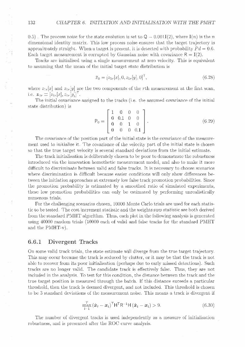
t32 CHAPTER, 6. INITIATIO¡\I A¡úD INITIALISATIO¡\T WITH THE PMHT
0.5) . The process noise for the state evolution is set to Q :0.001I(2), where I(n,) is the ndimensional identity matrix. This low process noise ensures that the target trajectory isapproximatelv straight. rñ/hen a target is present, it is detected with probability Pd, : 0.6.Each target measurement is corrupted by Gaussian noise with covariance R: I(2).
Tracks are initialised using a single measurement at zero velocity. This is equivalentto assuming that the mean of the initial target state distribution is
ro: [zbfrf ,0, zt,[y],0]t, (6.28)
where zv[r] and z¡[y] are the two components of the rth measurernent at the first scan,i.e. z¡ = l"rrlrl,"rrlal]' .
The initial covariance assigned to the tracks (i.e. the assumed covariance of the initialstate distribution) is
P0
100 0.10000
001
0 1
000
0.
(6.2e)
The covariance of the position part of the initial state is the covariance of the measure-ment used to initialise it. The covariance of the velocity part of the initial state is chosenso that the true target velocity is several standard deviations from the initial estimate.
The track initialisation is deliberately chosen to be poor to demonstrate the robustnessintroduced via the innovation homothetic measurement model, and also to make it moredifficult to discriminate between valid and false tracks. It is necessary to choose scenarioswhere discrimination is difficult because easier conditions will only show differences be-tween the initiation approaches at extremely low false track promotion probabilities. Sincethe promotion probability is estimated by a smoothed ratio of simulated experiments,these low promotion probabilities can only be estimated by performing unrealisticallynumerous trials.
For the challenging scenarios chosen, 10000 Monte Carlo trials are used for each statis-tic to be tested. The cost increment statistic and the weights sum statistic are both derivedfrom the standard PMHT algorithm. Thus, each plot in the following analysis is generatedusing 40000 random trials (10000 each of valid and false tracks for the standard PMHTand the PMHT-v).
6.6.1 Divergent TlacksOn some valid track trials, the state estimate will diverge from the true target trajectory.This may occur because the track is seduced by clutter, or it may be that the track is notable to recover from its poor initialisation (perhaps due to early missed detections). Suchtracks are no longer valid. The candidate track is effectively false. Thus, they are notincluded in the analysis. To test for this condition, the distance between the track and thetrue target position is measured through the batch. If this distance exceeds a particularthreshold, then the track is deemed divergent, and not included. This threshold is chosento be 3 standard deviations of the measurement noise. This means a track is divergent if
Tþf @, - æ,)rHrR-'H (ù, - *r) , 9. (6.30)
The number of divergent tracks is used independently as a measure of initialisationrobustness, and is presented after the ROC curve analysis.

6.6. SIMULATED TRACK INITIATIO¡\¡ PERFOR ,TANCE 1 '.)It)t)
6.6.2 Uniform Clutter DistributionThe first case considered is the ubiquitous uniform clutter distribution. fhe perfornanceof the three proposed initiation schemes is examined for two different rates of false detec-tions. The first of these corresponds to 10 clutter measurements per scan. This is quite alow concentration of false measurements, and all of the schemes have a fairly easy time indiscriminating between false and valid tracks. In this example there is little to distinguishthe different approaches. The estirnated ROC curve for each of the initiation schemes onthis relatively low false detection rate is shown in figure 6.7. The weights sutn and costincrement quality measures are shown as a dashed line and a dotted line respectively. ThePMHT-v performance is shown as a solid line.
The second clutter false detection rate corresponds to 50 clutter measurements perscan. The estimated ROC curves for this relatively high concentration clutter are shownin figure 6,8. As is expected, the performance of all approaches is degraded from thatobtained on the lower concentration clutter. Of the three approaches, the PMHT-v givesthe best performance, although the difference between it and the weights sum approach isnot significant. The cost increment approach gives significantly worse performance thanthe other two. This is a little surprising, since the cost increment approach is linkedto established Model Order Estimation techniques, whereas the weights sum approach ispurely an intuitive, ad hoc method. This performance is expected, however, if the natureof the two statistics is more closely examined.
6.6.2.I Relationship Between Cost Increment and'Weights Sum for a Uni-form Clutter Distribution
It may have been intuitively expected that the weights sum (being an ad hoc test) wouldgive the worst initiation results. Howevet, the cost function increment has worse perfor-mance. By manipulating the expression for the cost increment quality statistic, this resultcan be predicted.
In this experiment, there is only one target model, and one clutter model. If the targetmodel is removed, then the cost function is
Tnt
Ç(x) t t loe (,' ("*l*l)t:l r:7T
Ð"rloe#, (6.31)T:I
since all of the measurements have the same probability when the clutter pdf is uniformWith the target model, the cost function is
T
8 (x,x") : e', -rler" + t Ðrrr,loeC,'Tnt
t:l r:1.t:l
cQq I (X,X") - A(X)
T
Qi +D q^ + t D-r,,loe C/ - t n¡rog ÇtI
T r¿t
t:1 r:7
T
Thus
t:l
(6.32)
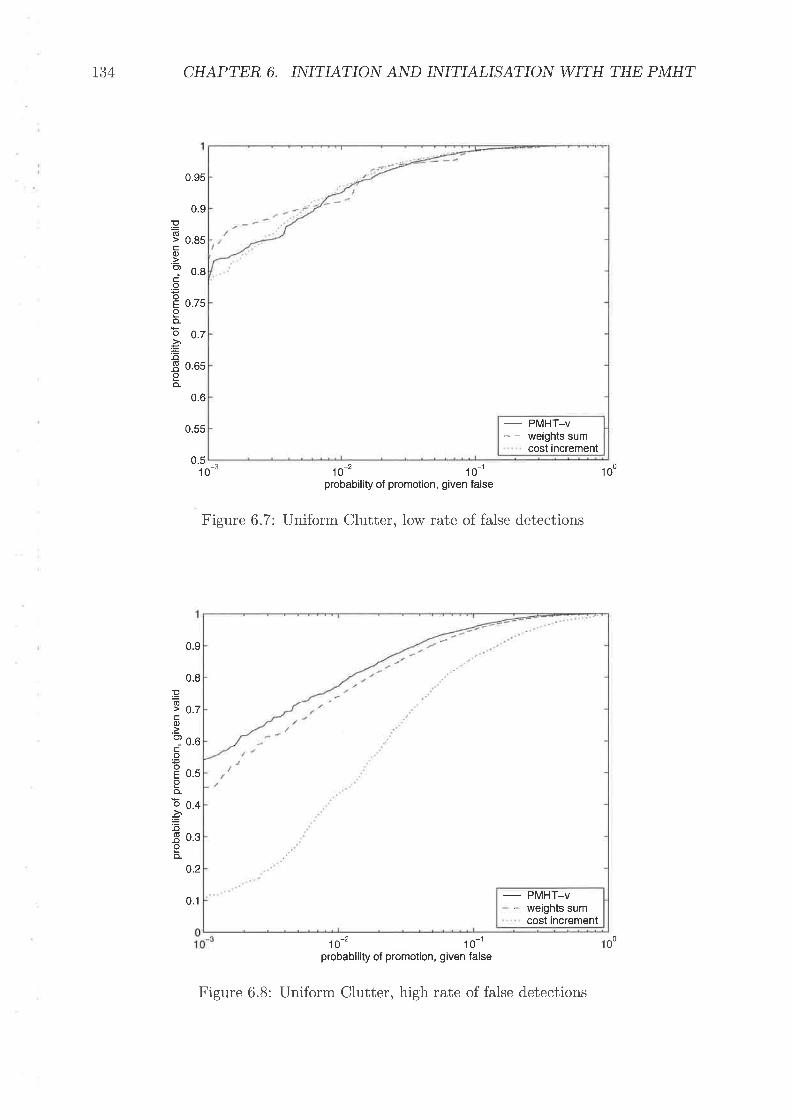
134 CHAPTER 6. INITIATIO¡\T A¡\ID INITIALISATIO¡ú WITH THE PMHT
-3
0.95
0.9pE o.asc.o
? o.aC.9
Ê o.zsooo 0.7àEE 0.65oo-
0.6
0.55
0.510
ol10 - 10 '
probability of promotion, given false
Figure 6.7: Uniform Clutter, low rate of false detections
D110 - 10 '
probability of promotion, given false
100
0.9
0.8pd> o.70)
? o.oco
Ê o.sIoo 0.4Èõ.3 0.3Io.
0.2
0.1
_ PMHT_V- - weights sum
cost increment
- PMHT_V. weights sumcost increment
Figure 6.8: Uniform Clutter, high rate of false detections
100
6.6, SIMULATED TRACK INITIATIO¡\I PERFORMANCE 135
(6.34)
T Tnt
t:l r:l
t-1 r:1TT
L
Ai +Ðq^+ t D tt - w,t,) log (,' - I n¿rog(|t:IT
t:Ir
t:7
ai+\,Q,*-tDr,*los#
ei +Ðq* -.,eelqi, (6.33)t:l
where Q', i" the model cost for the candidate track.The statistic clearly consists of a scaled version of the benchmark, qfi, plus two other
terms. The Q¡n term is relatively small and has secondary effect. The candid aLe lerm Q2,is negative definite since it consists of the sum of the norms of the random errors in themodel scaled by their corresponding covariances and by a factor of - |. fne assignmentweights also scale the measurement orientated error terms. The term proportional to q".
is positive definite since (1 < 1. Thus lhe Q2" acts against the qfl term. When the trackcorresponds to a valid target, it is likely that many measurements will be assigned to it,and this makes the Q2" term larger.
The cost increment statistic can be decomposed into two terms: the first term is thereduction in the clutter measurement cost due to assigning measurements to the candidatetrack. The second term penalises this cost improvement based on the discrepancy betweenthe candidate track and the assumed model. When the clutter is uniformly distributed,then the first term is simply proportional to the sum of the candidate assignment weights.However, when a non-uniform clutter distribution is present, the first term acts to reducethe quality statistic of tracks in highly cluttered regions and increase the quality statisticof those in sparsely cluttered regions. Thus the cost increment approach is more suitedto non-uniform clutter distributions.
6.6.3 Chi-Squared Clutter DistributionThe next clutter distribution considered is the chi-squared distribution with two degreesof freedom, i.e. an exponential distribution. This distribution is used in the E coordinatedirection, and a uniform distribution is used in the r coordinate direction. The clutterdistribution is thus given by
el Q',)1:
-€XD2000
As with the uniform distribution, two different rates of false detections are considered.Figure 6.9 shows an example trial. All of the measurements for the batch are shown in aspatial plot. The non-uniform distribution of clutter measurements in the vertical axis isclearly seen. The target is present in the trial, and the target detections can be seen inthe middle of the plot. The target rleasurements are shown as circles, and false detectionsAS CÏOSSES.
Figures 6.10 and 6.11 show the ROC curves generated for chi-squared distributedclutter. Again, the PMHT-v shows better performance than the weights sum. In thiscase, the performance difference is more significant than in the uniform clutter example.In contrast to the uniform case, the cost increment approach now performs almost as wellas the PMHT-v.
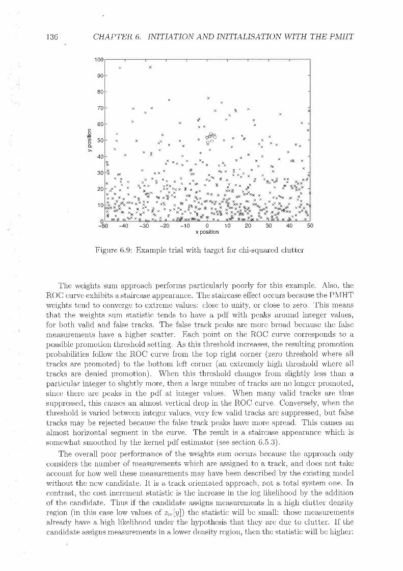
136 CHAPTER 6. INITIATIO¡\I A¡\ID INITIALISATION WITH THE PMHT
100
90
80
70
60c.9
850o_
40
30
20
10
-40 -30 -20 -10 0x position
10 20 30 40 50
Figure 6.9: Example trial with target for chi-squared clutter
The weights sum approach performs particularly poorly for this example. Also, theROC curve exhibits a staircase appearance. The staircase effect occurs because the PMHTweights tend to converge to extreme values: close to unity, or close to zero. This meansthat the weights sum statistic tends to have a pdf with peaks around integer values,for both valid and false tracks. The false track peaks are more broad because the falsemeasurements have a higher scatter. Each point on the ROC curve corresponds to apossible promotion threshold setting. As this threshold increases, the resulting promotionprobabilities follow the ROC curve from the top right corner (zero threshold where alltracks are promoted) to the bottom left corner (an extremely high threshold where alltracks are denied promotion). When this threshold changes from slightly less than aparticular integer to slightly more, then a large number of tracks are no longer protnoted,since there are peaks in the pdf at integer values. When many valid tracks are thussuppressed, this causes an almost vertical drop in the ROC curve. Conversely, when thethreshold is varied between integer values, very few valid tracks are suppressed, but falsetracks may be rejected because the false track peaks have more spread. This causes analmost horizontal segment in the curve. The result is a staircase appearance which issomewhat smoothed by the kernel pdf estimator (see section 6.5.3).
The overall poor performance of the weights sum occurs because the approach onlyconsiders the number of measurements which are assigned to a track, and does not takeaccount for how well these measurements may have been described by the existing modelwithout the new candidate. It is a track orientated approach, not a total system one. Incontrast, the cost increment statistic is the increase in the log likelihood by the additionof the candidate. Thus if the candidate assigns measurements in a high clutter densityregion (in this case low values of z¡,lE]) the statistic will be small: those measurementsalready have a high likelihood under the hypothesis that they are due to clutter. If thecandidate assigns measurements in a lower density region, then the statistic will be higher:
XX
X
xxX
Xx Xx xX
X X
XX
I
,i"x
XXX\tx
XXXXX l"
x& XXxX X Xx X a* xç x X xx Xx X xX X X XX X Xxx x XX XXX x Xx *.XXX Xx XX
xXX X N xxx XXX T& Xxx þ<)X XX XxXX x xX X xX ¡XX
XXX Xx 1i X
Xx
X X XtX x )?(X x XxX xXXx XXX Xx xxx¡X
X x X Xa x x XXf x X xx Xxx \ð,o Xxxl¡ax'x XXxX x*x xãx x X xXX *. XXXxgX
X x Xxìt ñXx Xx x X x)o(*X xXX ,lx x X"xx
Xx*X xxxX
t),<ry
Xñ
¡XX

6.6. SIMULATED TRACK INITATIOIV PERFORMANCE
0.1
1o-2 1o-1probability of promotion, given false
Figure 6.10: Chi-Squared Clutter, Iow rate of false detections
1o-2 1o-1probability of promotion, given false
t37
40
03
o2
prú
oo)
ooE
o-o=-o(ú-ooo.
0.9
0.8
0.7
0.6
0.5
1
100
100
0.9
0.8E(ú> o.7(¡)
? o.o.9
Ê o.so
o 0.4
=-o-8 0.3Io-
0.2
0.1
- PMHT_V
- - we¡ghts sumcost increment
I
_ PMHT_V- - weights sum
cost increment
Figure 6.11: Chi-Squared Ciutter, high rate of false detections
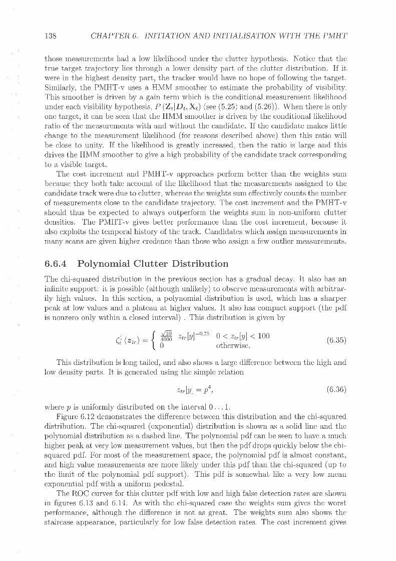
138 CHAPTER 6. INITIATIO¡\I A¡úD INITIALISATION WITH THE PMHT
those measurerrrents had a low likelihood under the clutter hypothesis. Notice that thetrue target trajectory lies through a lower density part of the clutter distribution. If itwere in the highest density part, the tracker would have no hope of following the target.Similarly, the PMHT-v uses a HMM smoother to estimate the probability of visibility.This smoother is driven by a gain terrn which is the conditional measurement likelihoodunder each visibility hypothesis, P (ZrlDr,X¿) (see (5.25) and (5.26)). When there is onlyone target, it can be seen that the HMM smoother is driven by the conditional likelihoodratio of the measurements with and without the candidate. If the candidate makes littlechange to the measurement likelihood (for reasons described above) then this ratio willbe close to unity. If the likelihood is greatly increased, then the ratio is large and thisdrives the HMM smoother to give a high probability of the candidate track correspondingto a visible target.
The cost increment and PMHT-v approaches perform better than the weights sumbecause they both take account of the likelihood that the measurements assigned to thecandidate track were due to clutter, whereas the weights sum effectively counts the numberof measurements close to the candidate trajectory. The cost increment and the PMHT-vshould thus be expected to always outperform the weights sum in non-uniform clutterdensities. The PMHT-v gives better performance than the cost increment, because italso exploits the temporal history of the track. Candidates which assign rneasurements inmany scans are given higher credence than those who assign a few outlier measurements.
6.6.4 Polynomial Clutter DistributionThe chi-squared distribution in the previous section has a gradual decay. It also has aninfinite support: it is possible (although unlikely) to observe measurements with arbitrar-ily high values. In this section, a polynomial distribution is used, which has a sharperpeak at low values and a plateau at higher values. It also has compact support (the pdfis nonzero only within a closed interval) . This distribution is given by
C| Q,,) : # ,r,la]-o''u o { zt [E] < 1oo0 otherwise.
(6.35)
This distribution is long tailed, and also shows a large difference between the high andlow density parts. It is generated using the simple relation
zr,lAl : pa, (6.36)
where p is uniformly distributed on the interval 0. . . 1.
Figure 6.12 demonstrates the difference between this distribution and the chi-squareddistribution. The chi-squared (exponential) distribution is shown as a solid line and thepolynomial distribution as a dashed line. The polynomial pdf can be seen to have a muchhigher peak at very low measurement values, but then the pdf drops quickly below the chi-squared pdf. For most of the measurement space, the polynomial pdf is almost constant,and high value measurements are more likely under this pdf than the chi-squared (up tothe limit of the polynomial pdf support). This pdf is somewhat like a very low meanexponential pdf with a uniform pedestal.
The ROC curves for this clutter pdf with low and high false detection rates are shownin figures 6.13 and 6.14. As with the chi-squared case the weights sum gives the worstperformance, although the difference is not as great. The weights sum also shows thestaircase appearance, particularly for low false detection rates. The cost increment gives
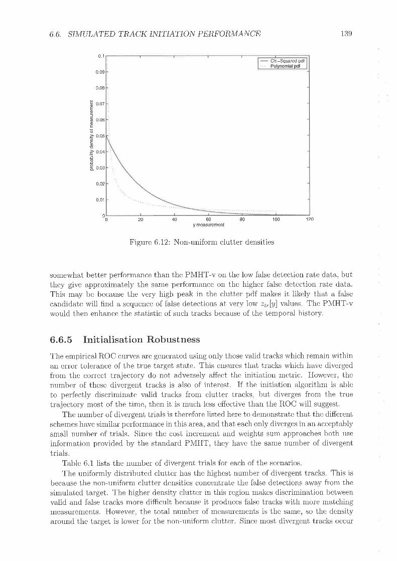
6.6. SIMULATED TRACK INITIATIO¡\T PERFORMANCE 139
coEo=(!oEo
coo=:õõooô
0.1
0.09
0.08
0.07
0.06
0.05
0.04
0.03
o.o2
0.01
00 20 40 60
y measurement80 100 120
Figure 6.12: Non-uniform clutter densities
somewhat better performance than the PMHT-v on the low false detection rate data, butthey give approximately the same performance on the higher false detection rate data.This may be because the very high peak in the clutter pdf makes it likely that a falsecandidate will find a sequence of false detections at very low z¡,lEl values. The PMHT-vwould then enhance the statistic of such tracks because of the temporal history.
6.6.5 Initialisation RobustnessThe empirical ROC curves are generated using only those valid tracks which remain withinan error tolerance of the true target state. This ensures that tracks which have divergedfrom the correct trajectory do not adversely affect the initiation metric. However, thenumber of these divergent tracks is also of interest. If the initiation algorithm is ableto perfectly discriminate valid tracks from clutter tracks, but diverges from the truetrajectory most of the time, then it is much less effective than the ROC will suggest.
The number of divergent trials is therefore listed here to demonstrate that the differentschemes have similar performance in this area, and that each only diverges in an acceptablysmall number of trials. Since the cost increment and weights sum approaches both useinformation provided by the standard PMHT, they have the same number of divergenttrials.
Table 6.1 lists the number of divergent trials for each of the scenarios.The uniformly distributed clutter has the highest number of divergent tracks. This is
because the non-uniform clutter densities concentrate the false detections away from thesimulated target. The higher density clutter in this region makes discrimination betweenvalid and false tracks more difficuit because it produces false tracks with more matchingmeasurements. However, the total number of measurements is the same, so the densityaround the target is lower for the non-uniform clutter. Since most divergent tracks occur
- Chi-Squared pdf
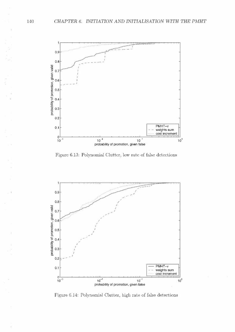
r40 CHAPTER 6. INITIATO¡\I A¡\ID INITIALISA?/O¡ü WITH THE PMHT
0.9
0.8põ> 0.7co? o.o.9
Ê o.so
o 0.4
=õ-8 0.3oo_
0.2
0.1
0
08
07
06
05
04
03
02
pEcc)
o)
.9oEIo_
o.=(ú-ooo-
10_t _l
10 - 10probability of promotion, given false
Figure 6.13: Polvnomial Clutter, low rate of false detections
0.9
0.1
0-3 1o-2 1o-1
probability of promotion, given false10
100
_ PMHT_V- - weights sum
cost increment
- PMHT_V
- - weights sumcost increment
Figure 6.14: Polynomial Clutter, high rate of false detections
100
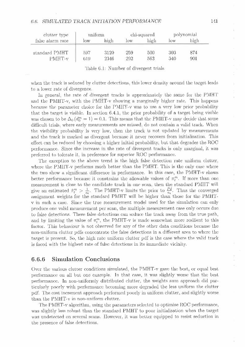
6.6. SIMULATED TRACK INITIATIO¡\I PERFORMANCE t47
clutter typefalse alarm rate
standard PMHTPMHT-v
uniformlow high
597619
chi-squaredIow high
3120 259 5002346 292 563
polynomialIow high
303340
874901
Table 6.1: Number of divergent trials
when the track is seduced by clutter detections, this lower density around the target leadsto a lower rate of divergence.
In general, the rate of divergent tracks is approximately the same for the PMHTand the PMHT-v, with the PMHT-v showing a marginally higher rate. This happensbecause the pararneter choice for the PMHT-v was to use a very low prior probabilitythat the target is visible. In section 6.4.1, the prior probability of a target being visiblewas chosen to be A6 (dT :1) : 0.t. This means that the PMHT-v may decide that somedifficult triais, where early measurements are missed, do not contain a valid track. Whenthe visibility probability is very low, then the track is not updated by measurementsand the track is marked as divergent because it never ïecovers from initialisation. Thiseffect can be reduced by choosing a higher initial probability, but that degrades the ROCperformance. Since the increase in the rate of divergent tracks is only marginal, it waspreferred to tolerate it, in preference for superior ROC performance.
The exception to the above trend is the high false detection rate uniform clutter,where the PMHT-v performs much better than the PMHT. This is the only case wherethe two show a significant difference in performance. In this case, the PMHT-v showsbetter performance because it constrains the allowable values of ri. If more than onemeasurement is close to the candidate track in one scan, then the standard PMHT willgive an estimated frf > *.The PMHT-v limits the prior t" #. Thus the convergedassignment weights for the standard PMHT will be higher than those for the PMHT-v in such a case. Since the true measurement model used for the simulation can onlyproduce one valid measurement per scan, the multiple measurement case only occurs dueto false detections. These false detections can seduce the track away from the true path,and by limiting the value of rl, the PMHT-v is made somewhat more resilient to thisfactor. This behaviour is not observed for any of the other data conditions because thenon-uniform clutter pdfs concentrate the false detections in a different area to where thetarget is present. So, the high rate uniform clutter pdf is the case where the valid trackis faced with the highest rate of false detections in its immediate vicinity.
6.6.6 Simulation ConclusionsOver the various clutter conditions simulated, the PMHT-v gave the best, or equal bestperformance on all but one example. In that case, it was slightly worse that the bestperformance. In non-uniformly distributed clutter, the weights sum approach did par-ticularly poorly with performance becoming more degraded the less uniforrn the clutterpdf. The cost increment approach performed poorly in uniforrn clutter, and slightly worsethan the PMHT-v in non-uniform clutter.
The PMHT-v algorithm, using the parameters selected to optimise ROC performance,was slightly less robust than the standard PMHT to poor initialisation when the targetwas undetected on several scans. However, it was better equipped to resist seduction inthe presence of false detections.

r42 CHAPTER 6. INITIATIO¡ú A¡üD INITIALISATION WITH THE PMHT
Overall, the PMHT-v, which is a special case of the PMHT-ym algorithm, is found tobe the preferred approach for track initiation out of those considered in this chapter.
6.7 SummaryThe standard PMHT is limited by the assumption that the number of targets is fixed andknown, and that prior information is available about the state of each. This chapter hasintroduced a method for making the PMHT robust to poor initialisation, due to inade-quate knowledge of this prior. This method uses the homothetic measurement model, butemploys a dynamic secondary measurement model specified by the innovation covariancematrix. This approach can be viewed as an automated covariance inflation method forinitialisation.
This chapter has also presented alternative methods for allowing the PMHT to usea dynamic number of target models. These methods are based on over modelling theproblem, and then rejecting superfluous models based on a model significance test. Thisapproach is referred to as candidate based track initiation, and each candidate track isassigned a quality statistic by the tracker. Two different tests were propose for use withthe standard PMHT. Firstly the candidate quality was quantified by using the sum ofthe assignment weights for that model. Secondly the candidate quality statistic was givenby the improvement in the EM auxiliary function when it was introduced. The PMHTwith Hysteresis was also used to provide a candidate quality mea,sure. The PMHT-ymwas implemented using a binary assignment model, and the probability of the assignmentstate was used as the candidate quality. This algorithm is referred to as the PMHT-vbecause the binary assignment model is analogous to the visibility approach used for trackinitiation with other algorithms. The PMHT-ye was also used, but not tested extensivelybecause it provided poor performance, even with a large state space.
The track initiation schemes proposed were tested on simulated data under a varietyof clutter conditions, and their performance quantified by ROC curves for the candidatetest. The PMHT-v (i.e. the binary PMHT-ym) method was found to consistently givegood performance over all conditions and is considered the preferred approach based onthese results.

Chapter 7
Applying the ProbabilisticMulti-Hypothesis Tracker to OverThe Horizort Radar
T,tARLItrR chapters have introduced theoretical extensions of the PMHT algorithm. TheI1 performance of these extensions has been demonstrated through simulations. How-ever) as with all things, the proof of the pudd'ing'is'in the eati,ng [dC05]. In this chapter,the PMHT extensions are applied to data recorded from the Jindalee Facility at AliceSprings (JFAS) Over the Horizon Radar (OTHR). The performance results obtained fromrecorded OTHR data are used to verify the simulated results of the previous chapters.
This chapter first reviews some basic principles of Over the Horizon Radar, with focuson some particular features of the JFAS radar pertinent to target tracking. Problemsencountered when processing JFAS data are discussed and the PMHT solution to theseproblems presented. ROC curves for track initiation are then estimated using recordedJFAS data.
The JFAS OTHR is an Australian operational sensor. For this reason, the radardata itself, and the performance of the radar algorithms cannot be presented in an openpublication. Instead, relative performance metrics comparing competing algorithms areused. Thus the performance measures, derived from radar data, presented in this chapter(in particular initiation ROC curves) deliberately do not show quantitative axis scales.
7.t Over the Elorizon Radar FundamentalsOver the Horizon Radar is the name given to a class of active radar sensors that exploitelectromagnetic refraction in the high frequency (HF) band. This refraction is used tocurve the signal propagation path and sense beyond the line of sight limitation of astandard radar sensor. Figure 7.1 shows how a curved propagation path can increase thedetection range of a radar.
Surface Wave radar is a form of OTHR that exploits refraction due to the sea. InSurface Wave radar, the radar signal hugs the sea surface because the media boundarybetween air and water curves the propagation path.
Skywave OTHR exploits a part of the atmosphere called the ionosphere. The iono-sphere is a cloud of ionised particles formed by the solar radiation. It is composed ofseveral regions of high ion density, referred to as layers. The elevation of these layersvaries as does their density and spatial extents. Each layer provides a potential propaga-
r43

r44 CHAPTER 7, APPLYING THE PMHT TO OTHR
Line of sight radar Over the horizon radar
Figure 7.1: Extended radar range through electromagnetic refraction
tion path between the sensor and targets of interest. Since target echoes may return bya different layer from the one that transported the transmitted signal, skywave OTHR isa multipath sensing environment with the number of possible paths given by the squareof the number of layers. There are other factors which also provide further propagationpaths. For example, when an aircraft flies over water, a Lloyd's mirror effect is experi-enced, and a signal may propagate not only due to direct backscatter from the aircraft,but also from backscatter reflected from the water beneath. In this case, the length of thetwo paths will differ only slightly, however the phases of the two paths will be different,and may cause fluctuations in the received signal por'¡/er.
A common condition for the JFAS radar is propagation support from two layers, calledthe E and F layers. Signals propagated via the E layer arrive more quickly than thosepropagated via the F layer, because of its lower altitude. Figure 7.2 shows how a twolayer environment provides four return paths to the radar. In standard OTHR parlance,each of the different return propagation paths is referred to as a mode, and the modesare labelled to show the layer which supported the transmitted and reflected signals. Thepaths for which the return propagation is via a different path to the transmitted signalare called mixed modes. Mixed modes which involve the same two layers in reverse order(such as the FE mode and EF mode in figure 7.2)have the same length, but arrive at thereceiver from different elevations. Since JFAS uses a linear receiver aruay, this causes thepaths to be observed at different azinuths. The observed azimuth for a linear array is thecone angle between the array and the incident signal, which is a function of the bearingand elevation angles.
A result of sensing targets at long range is that there is very high propagation loss whenbackscattered signals eventually return to the receiver. In order to detect these signals, thetransmitter power must be relatively high, and this requires a high duty cycle waveform.This restriction means that OTHR systems are built in a bistatic configuration withtransmitter and receiver beyond line of sight to prevent interference. Since the separationof the transmitter and receiver is small compared with the observation range, the systemcan be assumed to be approximately monostatic,
The transmitter waveform is a frequency modulated signal with a carrier frequencyranging from a few megahertz to tens of megahertz. Lower frequencies are refracted moreand are used to illuminate shorter ranges. Lower frequencies must also be used at nighttime when the ionosphere reduces in size without ionising radiation from sunlight. Theradar uses a stepped scanning strategy, which means that wide area coverage is achievedby tiling the surveillance area with smaller regions. The sensor dwells on each region fora period, collecting data over a number of waveform repetitions to measure target range,bearing angle and Doppler frequency shift. The sensor then steps to a different region

7.2. SPECIFIC OVER THE HORIZON RADAR MODELS 745
r: ny-eL - -'
Elaye¡-
EE mode FE mode
EF mode FF mode
Figure 7.2: Typical multipath propagation
and later revisits each previous region based on a scheduling scheme. Regions may havedifferent priorities and the revisit time (namely the time between consecutive looks foreach region) is region dependent and variable.
7.L.L Jindalee Facility at Alice SpringsThe JFAS OTHR is a skywave radar built by the Defence Science and Technology Or-ganisation (DSTO) to provide surveillance over the north western coast of Australia. Thetransmitter and receiver sites are located close to the city of Alice Springs in centralAustralia. This radar is operated by the Royal Australia Air Force (RAAF). Two sim-ilar radars at Laverton and Longreach have recently been commissioned. These sensorscomprise the Jindalee OTHR Network (JORN), providing coverage to the entire northernand western coast of Australia.
Archived data from the JFAS OTHR will be used in this chapter to confirm thesimulations presented in earlier sections.
A history of the development of the JFAS OTHR can be found in [Col00]. A technicaloverview of the signal processing algorithms used to process the radar data is given in[Lee87].
7.2 Specific Over the Horizon Radar ModelsThe particular target and clutter models used for this application are now presentedThese models will be applied in all cases where experimental data is analysed.
7.2.1 Measurement VectorThe JFAS OTHR uses a sequential signal processing approach. The received signal fromthe antennae is passed through successive data processing algorithms culminating in thetracking algorithm. Figure 7.3 shows the typical data processing algorithms applied tothe receiver data up to tracking. By the detection stage, the data has been converted
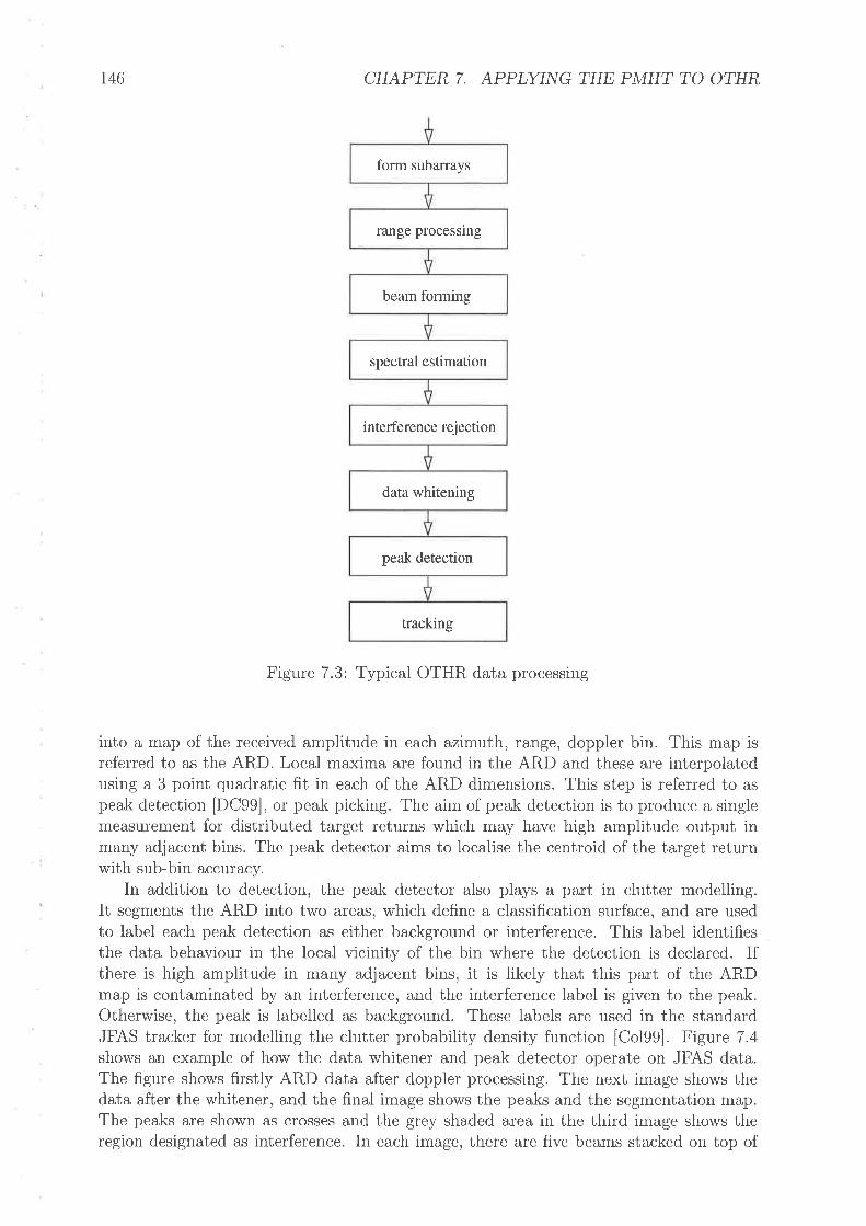
form subarrays
range processing
beam forming
spectral estimation
interference rejection
data whitening
peak detection
tracking
r46 CHAPTER 7. APPLYING THE PMHT TO OTHR
Figure 7.3: Typical OTHR data processing
into a map of the received amplitude in each azimuth, range, doppler bin. This map isreferred to as the ARD. Local maxima are found in the ARD and these are interpolatedusing a 3 point quadratic fit in each of the ARD dimensions. This step is referred to aspeak detection [DC99], or peak picking. The aim of peak detection is to produce a singlemeasurem.ent for distributed target returns which may have high amplitude output inmany adjacent bins. The peak detector aims to localise the centroid of the target returnwith sub-bin accuracy.
In addition to detection, the peak detector also plays a part in clutter modelling.It segments the ARD into two areas, which define a classification surface, and are usedto label each peak detection as either background or interference. This label identifiesthe data behaviour in the local vicinity of the bin where the detection is declared. Ifthere is high amplitude in many adjacent bins, it is likely that this part of the ARDmap is contaminated by an interference, and the interference label is given to the peak.Otherwise, the peak is labelled as background. These labels are used in the standardJFAS tracker for modelling the clutter probability density function [Col99]. Figure 7.4shows an example of how the data whitener and peak detector operate on JFAS data.The figure shows firstly ARD data after doppler processing. The next image shows thedata after the whitener, and the final image shows the peaks and the segmentation map.The peaks are shown as crosses and the grey shaded area in the third image shows theregion designated as interference. In each image, there are five beams stacked on top of

7,2. SPECIFIC OVER THE HORIZON RADAR MODELS t47
(7 4)
(7 3)
Figure 7.4: Data processing stages for the Jindalee OTHR
each other, and each beam is an image with range and doppler bins displayed verticallyand horizontally respectively.
The output of the peak detector is the input to the tracker, and so there are twomeasurement types. Firstly, the peak detections themselves are four eiement vectorscontaining observed range, doppler, azimuth and amplitude. Thus,
":? : lrnlrl, ztulldl, zr,l0l,
"r,lol]r . (7.1)
The second measurement is the discrete peak tags (interference or background). Theseclassification tags can be viewed as a set of augmented measurements, giving
(*)zir'(k)zir'
(7.2)-tr -
where "[p i, a binary variable denoting the class assigned to that peak
7.2.2 Target State RepresentationThere are two different types of state models used to represent targets in the OTHRenvironment. These two types correspond to two different types of targets observed bythe radar. The models are referred to as the coupled model and the decoupled model
[Col99]. The difference between the two models is in the treatment of the observedDoppler frequency shift, z¡,lf¿|.
In the coupled model, the Doppler frequency shift is purely caused by the movementof the target. The shift is proportional to the radial velocity of the target, according tothe standard Doppler shift equation
-2f.flac
where /¿ is the doppler shift, /" is the carrier frequency of the transmitted signal, r is theradial velocity of the scatterer, and c is the speed of light. The coupled model is used torepresent standard air targets.
In the decoupled model, the observed Doppler shift is not purely due to the targetmotion, but also due to an additive frequency shift at the target, or in the propagationmedium, _){ ;r oJc' t rJd---TJotc
+++
+
+ +r
+h**fr+
++

148 CHAPTER 7. APPLYING THE PMHT TO OTHR
where /, is the additive frequency shift. The decoupled model has an extended state spacewhich includes a frequency rnodulation parameter. The observed frequency shift is thesum of the Doppler frequency shift due to target motion and the frequency modulationshift. The decoupled model is used to represent transponders that use a mixer to modulatethe transmitted signal. These transponders are usually geographically fixed and are usedto infer ionospheric model parameters. However, they display apparent motion due totravelling ionospheric disturbances (waves in the ionosphere). These disturbances rnaycause variations in the elevation of arrival and the delay of the received signal, which isinterpreted by sensor as motion in azimuth and range. Range variations are usually small,but azimuth effects can be significant. The decoupled model can also be used to modelvery low speed targets, such as ships, where the Doppler frequency shift due to movementof the ionosphere may be significant compared with the Doppler frequency shift due totarget motion.
7.2.2.I Coupled Model
The main state model is the coupled model and is used for aircraft and sea targets (whenionospheric motion compensation is applied before tracking). It consists of an almostconstant velocity linear motion model in two dimensions: range and azimuth. The motionof most targets will not have constant velocity in the radar coordinate space, however itis a reasonable approximation to make at the long ranges encountered with OTHR. Theprocess noise is assumed to be sufficient to compensate for this mismatch. The state vectoralso contains the target amplitude, which is modelled as an almost constant feature ofthe target. Thus, the coupled state vector for the rnth target, rrl : Mv I I . . . M, is
"Tlrl, rTlrl, rTl0l, rTl0), "Tl"l\ (7 5)
The almost constant velocity model is presented in more detail in section 3.3. The stateevolution is assumed to be a linear process contaminated with white additive Gaussiannoise zf with covariance matrix Qi such that
æT : Ftæ\t -f G¿ui. (7 6)
The noise process ul contains three elements modelling acceleration in range andazirruth and fluctuations in signal level. The covariance matrix, Ql, is assumed to bediagonal.Thus, m r ruT:{"Tlrl,uTl0l,"Tl"l}, (7.7)
and lqrll o o IQi:l o aTlol o l, (7.8)
I o o aTþl)where the scalars QTlrl, QTl?l, and Qilal are design parameters.
The matrices F¿ and G¿ are determined by the equations of motion and are given by
00F(lD) 0
01
*T:{
F
0G(1D)
0
00
Tt - Tt-t
(7 e)
(7.10)

7.2. SPECIFIC OVER THE HORIZON RADAR MODELS t49
, and G(1D) :1t ,2i\rt - rt:) , as defined in section 3.3where F(1D) : I r¡-r¿
01 Tt - Tt-tThe measurement is assumed to be a linear process contaminated with additive white
Gaussian noise o¿" with covariance matrix R¿ such that
"Í? :HtæT I?)t, (7.11)
when k¿y : rTL indicates that ztl is due to target model rn.The noise process o¿. contains four elements corresponding to each of the four com-
ponents of the measurement vector. The covariance matrix of this noise is assumed to bediagonal. Thus,
ntr: {u*lrl,ur,lfa],ubl0l,ur,lo)}., (7.L2)
R¿:000
RTvol o oo RTlql 00ORT
(7 13)
where the scalars RTlrl, RTlf ol, RTl?l, and Rilal are design parametersThe matrix H¿ is given by
RT000
T
a,
1
H+: 0"00
ftt.?ls
000000100'001
c (7.14)00
where /- is the waveform repetition frequency, /" is the carrier frequency, c is the speed oflight, and A" is the range extent of each range bin. The coupling between the range anddoppler measurements occurs because both measurements are obtained from the phaselaw of the received signal. Notice that the azimuthal velocity is not observed and mustbe inferred from the progression of measurements over time. The doppler measurement isnot strictly linear because the velocity measurement is arnbiguous and some velocities arethus aliased. This is equivalent to a fixed offset which can be compensated. This aliasingis described in rrore detail in section 7.3.
7.2.2.2 Decoupled Model
The second target state model is the decoupled rnodel and is used for transponders and anartificially injected calibration signal used in the JFAS radar. Transponders are positionedat various known locations within the coverage area of the radar and are used to estimateionospheric model parameters. The transponder itself is a fixed device with a modulatorthat produces a frequency shift in the transmitted radar waveform. This frequency shift isobserved as a doppler frequency shift by the radar processing. Thus the observed dopplershift is independent of the target dynamics. Since the physical location of the transponderis known, tracks formed on transponders can be used as reference points for ionosphericmodelling, which is required to estimate the ground position of other radar targets.
The calibration signal is the other type of decoupled target. These signals are injectedinto the receiver subarrays at a fixed frequency modulation and in fixed range bins. Liketransponder signals, they are observed by the radar processing as targets whose dopplershift is independent of their (stationary) dynamics.

150 CHAPTER 7. APPLYING THE PMHT TO OTHR
As with the coupled model, the state vector contains amplitude. The model is identicalto the coupled model, except that it also contains a frequency modulation pararneter, r[f r].Thus the decoupled state vector is
(7.15)
The state evolution is the same as the coupled model, with the frequency rnodulationassumed to be a constant process contaminated with white additive Gaussian noise. Thenoise process ul contains four elements modelling fluctuations in range, azimuth, dopplerfrequency shift and signal level. These fluctuations may be caused by both random noiseand ionospheric disturbances, such as travelling waves. The covariance matrix of thisnoise is assumed to be diagonal. Thus,
uT : {"Tlrl,uTll"l,"Tl0l,rTlol}-, (7.16)
æT : {rT lrl, rT lrl, rT ll.), rT l0l, rT l0l, rT lol}
AT000
r 00QTV.] O0 STle)
00
0010o F(1D)00
000Tt-Tt-t 0 0
o G(lD) o0 0 Tt-Tt_t
000
QTl"
000'1
0000100001000001
o
G¿:
ITL
t (7.17)
(7.20)
(7 18)
(7.1e)
where again, QTlrl, Q?llal, QTlel, and Qilal are scalar design parameters. The de-coupled model uses lower values for the process noise parameters, because those targetswhich obey this model have sedate dynamics. In fact, any apparent dynamic behaviouris primarily due to ionospheric effects for targets of this type.
The matrices F¿ and G¿ are given by
F
F¿:
000
1( D )000
D1G (
The measurement model is the same as the coupled model, but with a measurementmatrix given by
H¿:1
000
fin,ft60
7.2.3 Clutter state modelThe distribution of clutter measurements in azimuth, range and doppler frequency ismodelled as uniform. A clutter state model is used to model the distribution of theamplitude of clutter measurements. The amplitude distribution for clutter measuretnentsis modelled as a mixture of two components in the current tracking system. Two cluttermodels will therefore be used for the analysis of recorded OTHR data in this work. Thesetwo components can be thought of as false measurements caused by fluctuations in the

7,3. INITALISING FROM AMBIGUOUS DOPPLER MEASUREME¡\ITS 151
background noise and false rneasurements caused by interference. Common interferencesources in the OTHR environment are meteors, range ambiguous spread doppler groundclutter and signals from other users of the HF band.
In the analysis to follow, the distribution of the amplitude of measurements from eachclutter model is assumed to be exponential. As stated above, the distribution in otherdimensions is assumed to be uniform. The clutter model state vector is a vector of theparameters of the assumed amplitude distribution which is a single parameter for theexponential distribution, i.e. æT = ri is a scalar for the clutter models. The clutterstate is assumed to be fixed over the batch. Thus the dynamics of the clutter modelrn : 1. .. My : 2 are modelled as
,þT ("T1"7,) : ô @T - r7r) , (7.2r)
where ô(.) is the Kronecker delta function, an identity function taking unity value at theorigin and zero elsewhere.
The probability density of clutter measurements is given by
ci e,.t*T): Ih.,.o { -t+t} (7 22)
where z¿ is the detection threshold which is assumed to be known, and ,,4, is the volumeof the surveillance region in the dimensions of azimuth, range and doppler frequency.
7.3 Initialising from Ambiguous Doppler Measure-ments
As described earlier, the measurement received by an OTHR consists of an observationof range, azimuth, doppler frequency and amplitude. The waveforrn parameters used forOTHR are typically in the medium waveform repetition frequency range. This meansthat both the range and doppler frequency measurements may be aliased.
The ambiguous range of the waveform is usually very large - nominally a few thousandkilometres. This means that the signal attenuation from targets at this range will be sohigh that range ambiguous targets will not be detected. The exception to this is clutterthat may be received from a double refraction through the ionosphere. This clutter willbe detected from a long range that becomes aliased onto the region of interest becauseof the ambiguous waveform. The clutter is detected where targets are not because thebackscatter from the sea surface is much greater than that of a target. Also, at longerranges, returns very close to the sensor may also be aliased. This interference is referredlo as range folded clutter. Typically, range folded clutter may also be spread throughthe doppler domain, making target detection problematic. Problems arising from rangefolded clutter and targets ambiguous in range can be resolved using a variable waveformrepetition frequency, as discussed in more detail below. No special efforts will be madewithin thc tracker to address ambiguous range measurements.
The ambiguous doppler of the waveform is a significant problem. Common waveformparameters result in a relatively low ambiguous doppler frequency. This means that thedoppler frequency measurement will suffer from aliasing. Figure 7.5 shows observed thedoppler shift as a function of target radial velocity and highlights the aliasing problem.The horizontal dotted line illustrates how several feasible target velocities might causean observed normalised doppler frequency of 0.3. The normalised doppler frequency is

752 CHAPTER 7. APPLYTNG THE PMHT TO OTHR
the actual frequency divided by the waveform repetition frequency, and the normalisedradial velocity is the actual radial velocity divided by the ambiguous velocity, uo*6 whichis proportional to the arnbiguous doppler frequency.
A result of the doppler aliasing is that the posterior velocity distribution is multimodal.Each possible unwrapping of the aliased doppler corresponds to a peak in the posteriorvelocity distribution. These unwrapped velocities (and hence the distribution peaks) areeach separated by the ambiguous velocity. Thus, the posterior distribution is comb-likein structure with the spread around each mode determined by the measurement noise.Knowledge of the dynamic constraints of physical aircraft can be used to form a priordistribution of target velocities. Combining this prior with the observed doppler frequencyand its measurement probability density gives the posterior probability density of thetarget velocity. Figure 7.6 illustrates an hypothetical posterior density given an observeddoppler frequency of 0.3. Peaks are seen in figure 7.6 where the corresponding radialvelocity \maps to the observation. The outer peaks are lower because they correspond torelatively high radial velocities that are considered unlikely. Further peaks might exist athigher velocities depending upon the ambiguous velocity of the waveform which definesthe spacing between adjacent peaks. For OTHR these higher velocity wrappings usuallycorrespond to infeasibly high target speeds.
For OTHR, the ambiguous doppler measurement is further complicated by the exis-tence of. stati,onary targets. Stationary targets are targets that do not physically rnovethrough space, but nevertheless produce an apparent doppler frequency shift, due to anadditive frequency offset at the target. These are modelled using the decoupled model de-scribed in section 7.2.2.2. The existence of stationary targets provides a second family ofunwrapped states - each with zero radial velocity, but varying aliased mixing frequencies.Just as physical constraints can be used to limit the number of unwrapped radial speedsconsidered, knowledge of the range of mixing frequencies used by transponders can beused to limit the number of stationary options considered.
A common technique to resolve the velocity unwrapping problem is to change thewaveform repetition frequency from scan to scan. This changes the ambiguous range anddoppler frequency, and hence the collection of unwrapped velocities. Only the correctvelocity will be a possible unwrapping for all repetition frequencies. The correctly un-wrapped velocity can then be determined by correlating the measurements over time. Thisapproach eliminates different dynamic models and different stationary models, however itdoes not distinguish between a moving target model at the correct unwrapping and thestationary model at the equivalent frequency shift. The only way to discriminate betweenthese is through the range history of the target measurements - i.e. whether the targetactually moves. This is best done in the tracker itself. So, it is necessary to integrate amethod for resolving the doppler ambiguity with the tracker.
The result of the ambiguity in the doppler measurement is that the initial state prob-ability density function, ,þi@T), is multimodal in the range rate and offset frequencydimensions. Let the index ¡;- designate which of the possible unwrapped velocity op-tions is the true target radial velocity. lt^ is an integer taking a value in the rangel...Mp,where Mristhetotalnumberof modesof theinitialstatedensity. Thedensity,þi @T; p,*) is now unimodal, and the state prior is given by
Mp
,þi @i): t ,þi @i; p*) Pt"^ 0"\ , (7.23)pm:r
where Pr- (p^) is the prior probability mass of the index, p-.

7.3. INITIALISING FROM AMBIGUOUS DOPPLER MEASUREME¡\ITS
-2 -1 5
153
0.5.¡l 3
._tcr 04U)
b os0)
d 0.2c)
- t-{
b o.rÀ*o^
€UËc)ì -o'rc)U)
o _o.2
a)ú)
*o -0.4
-0.5 15
Figure 7.5: Observed Doppler frequency shift due to aiiasing
-1 -0.5 0 0.5 . 1
normalised radial velocitv, ;l;vamÒ
-1 -0.5 0 0.5 1
normalised radial velocity, ;l;- udmö
2
2
1.8
1.6
1.4
3eÊ-
c'l'1 .2Oil
^=1.LYo.eH*
0.6
0.4
0.2
-2 -1.5 'L5
Figure 7.6: Posterior probability density of radial velocity
154 CHAPTER 7. APPLYING THE PMHT TO OTHR
The design decision is now whether to treat [t^ as an extra piece of missing data(and thereby rnarginalise it out of the maximisation step) or to treat it as a variable tobe estimated by the algorithm. There are two disadvantages of treating Lt* as missingdata. Firstly, it will result in the need to calculate assignrnent weights for each differentpossible value of lP. 'I'his increases the algorithm's computation requirements since manynÌore measurement density calculations must be made. These calculations are typicallythe most expensive part of the tracking algorithm. Secondly, the state estimate will be asuperposition of the Ai[, different possible states, weighted according to their probabilities.While each of these options is a viable state sequence, the superposition of many of thernis most likely not. Further, the different dynamic options for the model must all occupythe same state space for the superposition to be sensible, and this is not the case sincethe decoupled and coupled models have different state vectors. So, the algorithm is likelyto give a state estimate that is poor. This is the same problem that occurs with the MAPestimate of a discrete variable.
If p^ is instead treated as a pararneter to be estirnated, then there is only one set ofweights for each target model, and they are used to estimate ¡t"^. '|he estimated p"* for thenext iteration is that velocity that maximises the auxiliary function, namely the one withthe lowest measurement scatter. However, these weights are determined using a particularvalue of L( derived from the previous iteration (or from initialisation). This means thatthe measurements that receive high weights might not be the true target measurements,but rather false detections that happen to lie along the wrongly assumed trajectory. Thesemeasurements reinforce the incorrect initial assumption. So, the estimation approachsuffers from a bias towards whichever unwrapped velocity is initially assigned to themodel. This problem may be exacerbated in dense target or multi-path conditions whereit is more likely that measurements will be found along incorrect trajectories.
Both of the above approaches have undesirable features. These features arise becauseboth approaches use a single state sequence to estimate the target. Whilst the truetrajectory is a single sequence, it is one of a set of possible sequences and selecting thecorrect member of this set is the problem at hand. Another solution can be found by usingan alternative target model. The alternative model uses a mixture to describe the targetrneasurements. Each component of the mixture is one of the possible state sequences)and the mixing proportions of these components are the unknown prior probabilities,Pr^ (tt^). The prior probability will be estimated by the algorithrn and the hope isthat this prior will converge to unity for the value of p^ corresponding to the correctunwrapped velocity.
This model is somewhat like the homothetic measurement model described in chap-ter 3 and chapter 6. In the homothetic measurement model, the measurement density ismodelled as a mixture of cornponents with the same mean, but with different measure-ment variances. In this model, the components have the same measurement probabilitydensity function, but different means.
Two different approaches for ambiguous velocity unwrapping were implemented andtested on radar data. These approaches were to treat the index of the correct dynamicmodel as a parameter to be estimated, and the mixture approach described above. Themissing data option was not implemented since different state vectors are used for thedifferent rnodels.

7.3. INITIALISING FROM AMBIGUOUS DOPPLER MEASUREMENTS 155
7.3.I Estimation Approach for Velocity lJnwrappingThis approach is substantially the same as the standard P\4HT algorithm. What isintroduced in addition is a target dynamic index, which is to be estimated. On thefirst run, a particular value for this index is chosen - for example the target is initiallyassumed to be outbound with an unaliased velocity. This value is used to generate theinitial state sequence, which in turn is used to calculate the assignment weights. Oncethese weights are obtained, the estimated state sequence and dynamic index are chosento jointly maximise the auxiliary function. For each value of the index, a particular initialstate pdf is assumed, and a Kalman smoother run over the measurements. The newestimated index is then the one corresponding to the smoother output with the highestlikelihood (the maximum associated auxiliary value). The new state sequence is theoutput of the smoother, and the algorithm moves to the next iteration.
Thus the estimation approach consists of the following steps:
1. Initialisation
(a) Choose an initial unwrapped velocity index, p^(0).
(b) Initialise the state estimate sequence where æfr(o) 't determined by the indexp,^(o).
2. Calculate measurement assignment weights, ,n, using the standard PMHT defi-nition
3. Maximisation.
(a) For each index ltr* : 7 . ..M, determine the optimal state sequence using aKalman Smoother where æff is determined by p* , and synthetic measurementsand covariances are defined in the standard PMHT manner.
(b) For each index Lr^ : 7 . . . A[p determine the conditional likelihood of the op-timal state sequence, Qft(¡;-), using the target model dependent part of thestandard PMHT auxiliary function.
(c) Update the state estirnate sequence, X(i), by choosing the optimal sequencefor the index with the highest QT}t*), and select the updated velocity index,
lt^Q) , as the index of the highest QTjt^).
4. Repeat steps 2 and 3 until convergence.
7.3.2 lJnwrapped Velocity as a Mixture ModelRecall that the target dynamics follows one of M, known models, but that the particularone of which is unknown. Each of these component models has its own state, prior density,evolution density and measurement densitS' functions. Let the state of the pth componentof target model rn at scan ú be denoted as æle. The state of model rn at scan ú is the setof all component states
æl = {*T',*T',...*f''). (7.24)_-¿ L J
Each component has its own measurement and evolution probability densities,
#' (rr,l*To), ,þfo @Tol*Yr), and tþ{e (*T').
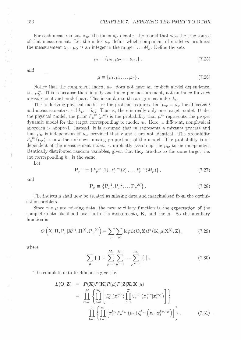
156 CHAPTER 7. APPLYING THE PMHT TO OTHR
For each measuremelí, z¿r, the index k¿" denotes the rnodel that was the true sourceof that measuretneut. Let the index ¡-r,¿, define which component of model m producedthe measurernent ztr. I,t* is an integer in the range L... A[p. Define the sets
pt = {Lttt, 11t2,.. . Ft r}, (7 25)
and
þ={h,pz,...pr}. (7.26)
Notice that the component index, ¡-r,¿r, does not have an explicit model dependence,i.e. þT. This is because there is only one index per measurement, not an index for eachm.easurement and model pair. This is similar to the assignment index k¿".
The underlying physical model for the problem requires that p"¿, : lf,t" for all scans ú
and measurements r,s if kr,: kr,. That is, there is really only one target model. Underthe physical model, the prior Pr* (tt^) is the probability that ¡t^ represents the properdynamic model for the target corresponding to model m. Here, a different, nonphysicalapproach is adopted. Instead, it is assumed that m represents a mixture process andthab ¡t¡, is independent of ¡;¿, provided that r and s are not identical. The probabilityPr* (p*) is now the unknown mixing proportions of the model. The probability is in-dependent of the measurement index, r, implicitly assuming the þ* Io be independentidentically distributed randorn variables, given that they are due to the same target, i.e.the corresponding k¿, is the same.
LetP r* = {Pr^ (I) , Pr^ (2) ,. . . Pr^ (Mò} , (7.27)
andpr= {prt,prr,...prr}, (7.2s)
The indices p shall now be treated as missing data and marginalised from the optimi-sation problem.
Since the p are missing data, the new auxiliary function is the expectation of thecomplete data likelihood over both the assignrnents, K, and the p. So the auxiliaryfunction is
O (*, rI, P,lx(t), fr(?), P/,(c)) : I I to* L(o,z) p (x, ¡,r,1x1) ,z) ., (T .2s)tL' K
whereM,, M,, M,,IÛ=Dt D Û
I,r ttl:I t-t2:I pLI :l
The complete data likelihood is given by
P(x) P(K) P (p) P (zlx, K, p)
(7.30)
: fr_{El* ør, t Err, @r, -y)l}
ú {I lnf* r,r* (t,,,)e!" ('* *f""')l\
L(O,Z)
(7.31)

7,3. /¡üI?IA¿ISI¡\IG FROM AMBIGUOUS DOPPLER MEASUREME¡\ITS
KT
Using the same simplifying steps as in section 4.L3, the conditional probability of theindices K and ¡; is given by
P (K, plX,Z) L(O,Z)f (x{i),2)
P(x) P(K) e QL,) e QlX, K, p)
t t r(xt¿) ¡ r1e e Qt) r (zlx,K, ¡t)
r57
(7.34)
(7.32)
(7.33)
p
il rtVf" Prr" (t r,) e!" (.r,1*f"-)]t:l r:L
t t il fÎ lnf*',r* (t''*) ef" ('nl*y""')f¡.t I{ t:7 r:l
Hprn
Tnt
il il u^pt l*:¡,rp:tf,*7t:l r:l
where the superscript (z) has been omitted from X, fI and P, to slightly simplify nota-tion. The weight umptr is implicitly dependent on these estimates from the previous EMiteration.
Following the steps set out in section 4.1..5, the auxiliary function can now be writtenAS
O (*, fI, Pplx(t), fr(i), Pp(¿)) log [P(x) P ($ e Qt) e (zlx,K, p)]
Tnt
Jl fl u¡nptrl^:¡,,,,p:¡",,t:L r:l
MMp
m:l p:I
M T
tt QT +D,qf +IQ,,,,ln:I t:l
where
QT : Iosrþio (*io) + t I"srþio (*T'l*Y) + t D*^rr,Iosefo Qr,l*To), (7.35)T
t:7
T rlt
t:I r:l
Qi : I to* Pr* (p)t I'u)rnptrtMp
P-I
TLT TLT
t:7 r:1(7 36)
and
umptr (7.37)
Apart from trivial notational differences, (7.35) is identical to the standard PMHTmodel expression for Q!, given in (a.28) and is optimised in the same way. As shown in
M fuIp nt
Qrn: I to* "f ÐDm:l p:L r:I

158 CHAPTER 7. APPLYING THE PMHT TO OTHR
section 4.L.5, the solution for the states r'fp can be realised using a Kalman Smootherwhen the statistics are linear and Gaussian. The important result in (7.34) is that thestate sequences of each of the components of model m can be estimated independently.
Similarly, (7.37) varies only slightly from the standard PMHT expression, given in(4.29). Using a Lagrangian approach, as in section '11.5, it is simple to show that opti-mising (7.37) gives the updated prior
Mp nt
tt umptr
rT: ++-^ (7.38)
IIY,,o,,The expression for Qff in (7.36) is again ahnost identical to @.29) and can easily be
shown to be optimised by ,1, nt
It wmptr
Pr*(P):
s:l p:I r-l
t:l r:IMpTnt
ttD.,,,.s-1 t:l r:1
(7.3e)
When the algorithm converges, the component with the highest Pr*(p) can be chosenas the dynamic model for target model m and the state estimate is given by fhe riesequence for that component. Prior knowledge (or belief) about the prior probability ofparticular target velocities can be incorporated though the initial values of the Pr. Inparticular, setting Pp^(o)(ù :0 for a specific component will result in Pr*(p): 0 forthat component on convergence.
This approach significantly increases the computation requirements of the algorithm,since each target model now has Mrweights per measurement and requires M, parallelKalman Smoothers for state estimation. This increased cost is sirnilar to that incurredby the PDAF approach for resolving the ambiguous velocity problem, given in [Col99].
7.3.3 Doppler lJnwrapping PerformanceThe two above approaches were implemented and run over a collection of JFAS data sets.The data used has a higher than average update rate (a small time delay between scans).This makes the doppler ambiguity problem more difficult because there is little time toobserve target motion. The fraction of correctly unwrapped tracks is shown in table 7.1.The trials were conducted for various batch lengths - longer batches provide more time forthe target to move and hence make velocity resolution easier. However, with a real-timesensor, the batch length should be limited to enable speedy track initiation.
The results in table 7.1 show that the estimation approach gives much better perfor-rnance than the mixture model. The performance of the estimation approach is almostconstant with batch length, which allows for the use of a short batch. As stated above,this is desirable for timely response of the tracker.
This result may be somewhat surprising - intuition suggests that the hard decisionmade in the estimation approach might cause the performance to be poor. In practice,the estimation approach is better because it incorporates the state likelihood as well asthe measurement likelihood. The mixture approach makes a decision based on the rela-tive probability of each component. This probability is determined by the measurernent
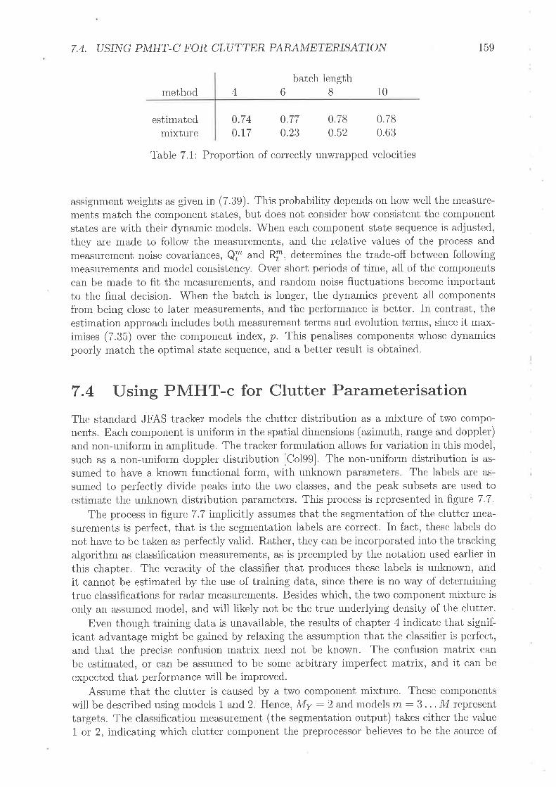
7.4. USI¡úG PMHT-C FOR CLUTTER PARAMETERISATION 159
method 4batch length
68 10
0.74 0.77 0.78 0.780.t7 0.23 0.52 0.63
estimatedmixtrrre
Table 7.1: Proportion of correctly unwrapped velocities
assignment weights as given in (7.39). This probability depends on how well the rneasure-ments match the component states, but does not consider how consistent the componentstates are with their dynamic rnodels. When each component state sequence is adjusted,they are made to follow the measurements, and the relative values of the process andmeasurement noise covariances, Qi and Rf , determines the trade-off between followingmeasurements and model consistency. Over short periods of time, all of the componentscan be made to fit the measurements, and random noise fluctuations become importantto the final decision. When the batch is longer, the dynamics prevent all componentsfrom being close to later measurements, and the performance is better. In contrast, theestimation approach includes both measurement terms and evolution terms, since it max-imises (7.35) over the component index, p. This penalises components whose dynamicspoorlv match the optimal state sequenceT and a better result is obtained.
7.4 Using PMHT-c for Clutter ParameterisationThe standard JFAS tracker models the clutter distribution as a mixture of two compo-nents. Each component is uniform in the spatial dimensions (azimuth, range and doppler)and non-uniform in amplitude. The tracker formulation allows for variation in this model,such as a non-uniform doppler distribution [Col99]. The non-uniform distribution is as-
sumed to have a known functional form, with unknown parameters. The labels are as-
sumed to perfectly divide peaks into the two classes, and the peak subsets are used toestimate the unknown distribution parameters. This process is represented in figure 7.7.
The process in figure 7.7 implicitly assumes that the segmentation of the clutter mea-surements is perfect, that is the segmentation labels are correct. In fact, these labels donot have to be taken as perfectly valid. Rather, they can be incorporated into the trackingalgorithm as classification measurements, as is preempted by the notation used earlier inthis chapter. The veracity of the classifier that produces these labels is unknown, andit cannot be estimated by the use of training data, since there is no way of determiningtrue classifications for radar measurements. Besides which, the two component mixture isonly an assumed model, and will likely not be the true underlying density of the clutter.
Even though training data is unavailable, the results of chapter 4 indicate that signif-icant advantage might be gained by relaxing the assumption that the classifier is perfect,and that the precise confusion matrix need not be known. The confusion matrix canbe estimated, or can be assumed to be some arbitrary imperfect matrix, and it can beexpected that performance will be improved.
Assume that the clutter is caused by a two component mixture. These componentswill be described using models 1 and 2. Hence, My :2 and models m:3 . . . M representtargets. The classification measurement (the segmentation output) takes either the valueI or 2, indicating which clutter cornponent the preprocessor believes to be the source of

data whitening
peak detection clutter segmentation
clutter parameterestrmatlon
tracking
160 CHAPTER 7, APPLYING THE PMHT TO OTHR
raw image
normalised scaling map
peaks peak classification
clutter model parameters
Figure 7.7: Clutter Segmentation Process
the corresponding state measurement. This means that the confusion matrix will not besquare; there are two observable classes, but M models. This is because the classificationmeasurement provides no information about targets.
Assume that the confusion matrix is of the form
c-The current approach treats the classification information as perfect, which is equiv-
alent to assuming that o1 : e.2: 7.
The feature used for classification is a measure of the local noise floor. The proba-bility that a target measurement will give rise to a classification ,Íf) :1 is therefore theproportion of the surrounding surveillance region with a local noise level correspondingto clutter model 1. This proportion can be approximated by the mixing proportions ofthe clutter components, and p is assumed to be given by
r!p nt (7.4r)
I (d +r?)
Q,1
r-c-tI-o.z
A2
pr-13 1 p
13 (7.40)
tt:l
t:I
The problem can now directly be approached as one of the form solved by the PMHT-calgorithm presented in chapter 4. The value of the classifier veracity, a, can be estimated,or simply assumed to be a particular number.

Classifier
Tracker
7.4. USING PMHT-C FOR CLUTTER PARAMETERISATION
ZU) 7(n)
7@)
Figure 7.8: Distributed Fusion Model
161
7u)7@)
Figure 7.9: Centralised Fusion iVlodel
7.4.I Centralised Fusion OptionUsing the PMHT-c algorithm to incorporate the classifier output can be viewed as adistributed data fusion approach. The sensor receives state observations and featureinformation. The feature information is used as the input to a classification algorithmthat in turn acts as input to the tracker. This architecture is shown in figure 7.8. Foreach measurement, tti) , th"r" is a corresponding feattne, zld) . The set of all featureinformation is labelle ¿ u, 7U) .
An alternative to this strategy is to feed the feature information as a direct input tothe tracker. The feature itself becomes a form of augmented measurement. The trackerthen assumes a probabilistic model for the distribution of the feature for each model, andit can be used in much the same way as the amplitude measurement. This architectureis shown in figure 7.9.
In th.e centralised architecture, the tracker jointly performs the tasks of classificationand state estimation. Since the tracker has access now to the feature data, rather thansimply a binary decision from the classifier, it is expected that the performance of thealgorithm will improve. Some of the decisions in the classifier will be indisputable whileothers are borderline. By coupling the classification decision into the tracker, the trackergains knowledge about the strength of the evidence for class assignments and this willimprove performance. If the classifier instead provided probabilities of each class, theuthere would be no advantage to the centralised approach.
The viability of joint classification and tracking in the form shown in figure 7.9 de-pends on the features and how much information is available about their distribution.The centralised architecture concatenates the features and the state observations to formaugmented measurements. For the tracker to be able to use the augmented measutements,the probability density of the each feature for each class must be known, or estimated.
The feature that is used in the Jindalee OTHR (a measure of the local noise floor) isa continuous valucd scalar and its distribution is unknown. However, the feature valuesfor all measurements were collected together and used to produce a kernel estimate ofthe probability density of the logarithm of the feature. This density estimate is shownin figure 7.10. The figure shows the estimated density for two different data sets. Thefirst data set contains relatively benign clutter, and the second data set contains morechallenging clutter caused by range folded spread clutter. In each case, the distributionis multimodal, but the positions of the modes is different. Also the variance of the
Tracker

762 CHAPTER 7. APPLYING THE PMHT TO OTHR
x 10 -
0.9
0.8
o.7
à06co-d.Êoso.¿õþ o+
03
o2
01
00 1000 2000 3000 4000 5000 6000scaling feature
7000 8000 9000 10000
Figure 7.10: Estimated feature pdf, p -u)
distribution is much higher for the interference data than the benign data.The two different feature densities in figure 7.10 can each be approximated as a two
component Gaussian mixture. As observed above, the variance of the components is muchhigher in the interference data, and the means are farther apart. So it is necessary to usea dynamic feature pdf which will adapt to the data. The bimodal nature of the densitiesin flgure 7.10 suggests that two different processes are at work, and was the motivationfor the original decision to use a two component model for clutter in the JFAS tracker.
Past analysis of the feature data and the measurement amplitude data has shownthat high values of the feature correspond to regions contaminated by interference wherethe amplitude distribution is more spread [RCID97, RC98]. Thus, it is reasonable toattribute the rightmost peak of the feature distribution to interference measurernentsand the leftmost peak to benign background measurements. Each clutter component isassumed to give rise to features which have a Gaussian distribution. The means andvariances of these two Gaussians are dynamic unknowns, but are assumed to be constantover the measurement batch.
Thus the clutter state vector lor m: 1,2 is now
æT = an : {"*1"],r^ltÀ,r^[o']]', (7.42)
where ,*lo] is the parameter of the exponential distribution for measurement amplitude,and r*l¡L,l and r^lo2] are the parameters of the Gaussian feature pdf. The augmentedmeasurement pdf is
(
11: -- €Xl)A r^lal
(4{, -,^tÀ))(7 )
benign datainterference data
ei Q*l*T) 2r^lo2)
43

7.4. USI¡\rG PMHT-C FOR CLUTTER PARAMETERISATIO¡\¡ 163
(7.44)
where it has been assumed that the feature measurement is independent of the amplituderneasurement.
The clutter state components are then estimated using their Maximutn LikelihoodEstimators (MLEs) given weighted measurements. These MLEs for the feature parametersare the weighted sample mean and variance given by
û^lpl:
Tnt
tt'"",,"1{)t:\ r:I
Tnt
ÐD,*,,t:l r:l
and
iË .**("Í{)-t^tpl)î*lo2l: t:7 r:I (7.45)Tnt
DÐ,^,,t:7 r:1
The feature pdf of target measurements is assumed to be a mixture of the clutterpdfs, where the two components are weighted by the estimated mixing proportions of theclutter models. The state observation is assumed independent of the feature. Thus fortargets,
p(ztulæT):Ç(,Íî,1*T)p(':{'), (746)
where
o(4{'): hn(,Í{)tt') * ffi'(,Í{'te'¡ 3 47)
7.4.2 Simulated Performance of PMHT-c for Clutter Parame-terisation
The performance of the various approaches for incorporating the clutter feature infor-mation is first investigated through simulations. These simulations are similar to thethose used to compare initiation methods in chapter 6. As with the analysis in chapter 6
the performance of the competing approaches will be compared using an experimentalinitiation ROC curve. For all cases, PMHT-v method is used for track initiation.
The measurernent space is two dimensional, as before, but now the measurements areaugmented with a third observation which provides classifrcation information about theclutter. This observation is the feature measurement.
Two alternative processing schemes are considered. The first method is the distributedfusion process described in the previous section. Under this approach, the feature mea-surement is thresholded to provide a binary estimate, indicating which clutter componentis associated with the measurement. This is analogous to the current JFAS process-ing. Thus the feature measurement, z[{), is converted to a classification measurement,,lp. fft" PMHT-c is then used., as outlined. in section 7.4. Three forms of the PMHT-care considered. Firstly, the classifier veracity is assumed to be perfect (*r: az: I),,which is analogous to the current JFAS approach. Next, the veracity is assumed to be(xr : a2: 0.9, and thirdly, it is estimated. The analysis in chapter 4 suggests that thesecond of these three will provide the best performance.

t64 CHAPTER 7. APPLYING THE PMHT TO OTHR
uninformative medium perfectr^ r^ rm' tr* r^ ,o' tr* :tr* to'
cluttercomponent
model 1
model 22
1
1
7
00
1
1
-2.50.5
-2.50.5
0.10.1
Table 7.2: Clutter parameters
The second processing scheme is the centralised fusion approach described in the pre-vious section. Here, the feature itself is simply treated as a third measurerr.ent dirnension.The target is assumed to have a mixture distribution in the feature domain, where thecomponents of the mixture are the two clutter distributions and the mixing proportion isderived from their relative frequency, namely p as defined in section 7.4.
Finally, two reference curves are generated. For the first curve, the tracker is providedwith perfect classification information (at least between the clutter distributions). Thiswill then give the best performance attainable by any of the other approaches. The secondcurve is the performance obtained using the standard PMHT algorithm, which effectivelyignores the classification information, This provides a benchmark; performance worse thanthe standard PMHT with useful classifications would be a poor result for any approach.
The measurements used in the simulation are random realisations of the two compo-nent clutter process, and target measurements (when it is present and detected). Perfor-mance is quantified through ROC curves, and the scenario is chosen to make initiationdeliberately difficult to bring out differences in the approaches.
The two dimensional measurement vector is denoteaiby zti) = {rr,lrl,zr,[E]]t Forboth clutter components, the measurement vector is uniformly distributed in z¿r[r), ex-ponentially distributed in z¿,lyl and has a Gaussian distributio"i" r!{). The exponentialparameters (namely the means) are fixed, and the Gaussian parameters are varied toachieve different classification veracities. Three different classifler veracities are consid-ered: uninformative classifications, medium veracity classifications, and perfect classifica-tions. These parameters are summarised in table 7.2. The clutter state vector is given bysm : {"^lAl,r*lp],r*[o']]', where r^lA] is the parameter of the exponential distribu-tion for the E coordinate measurement, and ,*lpl and r*[o2] are the pararneters of theGaussian distribution for the feature measurement.
As given ín Q.a7), the target feature distribution is a mixture of the clutter distribu-tions, when the target is present. The target dynamic model and measurement processare the same as that used in the initiation comparisons of chapter 6. Namely, the targetuses an almost constant velocity model with independent velocity perturbations in lhe rand y coordinate directions.
When the classifier is used., it thresholds the ,rf) *"u.urement at 0. In the unin-formative example, both classes have equal probability of being labelled class 1 ot 2, so(tr : u2: 0.5. In the medium veracity case, the classification veracities can be obtainedby integrating the "ll pdf over the decision region, and are ar : 0.95 and. a2: 0.76. Inthe perfect classification case, et : cuz - L.
The mixing proportions of the components are chosen so that three quarters of theclutter measurements are due to component 1. So, when no target is present, irl :0.75and rl :0.25.

7.4, USI¡úG PMHT-C FOR CLUTTER PARAMETERISATION 165
0-D _1
10 - 10probability of promotion, given false
10010
Figure 7.11: PMHT-c for clutter parameterisation, uninformative classifications
7.4.3 Simulation ResultsROC curves measured for the three feature distributions are now presented. In each case,the performance of the PMHT-c based algorithms is at least as good as the standardPMHT. The adaptive PMHT-c performs better than assuming perfect classifications) orassuming a : 0.9. The centralised fusion algorithm performs better than the PMHT-c.This centralised algorithm is only available because the pdf of the feature is a knownfunction. In many practical cases) this algorithm may not be realisable.
7.4.3.L lJninformative Classification
The ROC curves for the case of an uninformative feature are given in figure 7.11. Underthis condition, it is not expected that any of the llew approaches will perform betterthan the standard PMHT. There is no extra information available to exploit. The perfectclassification curve is still shown to give a performance bound. The PMHT-c algorithmwhich assumes a diagonal confusion matrix gives very poor results. This is because itis assuming that useless information is faultless. The other approaches all give roughlysimilar results, with no significant differences. The central fusion algorithm is slightlybetter than the others, and the PMHT-c which assumes that the classifier veracity isa : 0.9 is slightly worse. The PMHT-c which estimates the confusion matrix, and thestandald PMIIT (wliich does not use the classification measurements) give almost exactlythe same performance. This tends to indicate that the estimated a is behaving correctly.
7.4.3.2 Medium Veracity Classification
The ROC curves for the medium veracity example are given in figure 7.12, This case is themost interesting because it demonstrates the differences between the various approaches.
0.9
0.8p(ü> 0.7co)
? o.oc.o
E 0.5
!:,0.4='õ3 o.so_
0.2
0.1
')
,/
,' / '.' ),,ri'
/ z'
..: /,'t' . /,';'.
Pedect ClassificationCentral FusionEstimated aAssume a=1Assume ü=0.9standard PMHT
166 CHAPTER 7. APPLYING THE PMHT TO OTHR
The PMHT-c algorithm which assumes a : I actually degrades the performance overthe standard PMHT. Thus, assuming the classifications to be perfect is more detrimentalthan discarding them cornpletely. The adaptive PMHT-c has better performance. How-ever, assuming the veracity to be a : 0.9 is superior. This is in accordance with theresults reported in chapter 4, where assuming a : 0.9 appeared to be a sound strategy,independent of the true veracity. The centralised fusion algorithm performs better thanthe adaptive PMHT-c because it has access to the feature information which is a muchricher source than the classiflcation nìeasurements, however it has the same performanceas the PMHT-c with o : 0.9. This result is somewhat surprising; intuition would predictthat the centralised algorithm would be a clear winner. It indicates that the classificationsadequately summarise the feature data, for the purposes of this problem.
7.4.3.3 Perfect Classification
The ROC curves for perfect classification accuracy are given in figure 7.13. AII of thealgorithms have very similar performance to the reference curve for perfect classificationknowledge, because all have this knowledge. The adaptive PMHT-c, which estimates o,does slightly worse that the others. The PMHT performance is significantly worse, sinceit ignores the classifications.
7.4.4 Summary of Clutter Modelling \vith PMHT-cThe standard JFAS processing gives rise to feature measurements which the JFAS trackeruses to segment the state observations into background and interference classes. Thissegmentation step is a classification process where the class output is a binary randomvariable. The JFAS tracker assumes that this classification information is error free anduses it to estimate the parameters of a two component clutter model, and to identifywhich component of the clutter is the source of each measurement if it is not due to atarget.
The PMHT-c provides a framework for incorporating this classification informationwhich allows for errors in the classifier. Since the true confusion matrix of the classifieris unknown, the PMHT-c must either assume a particular confusion matrix, or estimateit from the data. Both of these possibilities were considered, with different assumedconfusion matrices. The algorithm with an assumed confusion matrix of the identitymatrix is analogous to the JFAS approach which assumes that the classifications arecorrect.
An alternative approach was identified whereby the classification step is removed com-pletely, and the tracker instead uses the feature information directly. Under this approach,the tracker must assume distributions for the feature data for clutter and target measure-ments. Empirical data
The various PMHT based approaches for clutter modelling were simulated and theirrelative performance observed via track initiation ROC curves. It was seen that thePMHT-c which assumes a non-ideal confusion matrix, and the PMHT-c with an estimatedconfusion matric both gave performance benefit over the standard PMHT which ignoredthe classification information. The PMHT-c which assumed the classifications were alwayscorrect performed worse than the standard PMHT - it was more detrimental to assume theinformation was perfect than to ignore it. The approach which fed the feature informationdirectly to a standard PMHT algorithm gave the best performance of the approachesconsidered.

7.4. USI¡úG PMHT-C FOR CLUTTER PARAMETERISATTON
0.9
t-110- 10'probabil¡ty of promotion, given false
100
Figure 7.12: PMHT-c for clutter parameterisation, medium veracity classifications
0.9
t67
08p(ú
z 0.7o? o.oc.9
E 0.5oo_
3.0.4E
.8 o.so
0.2
0.1
I0p(ú> 0.7cc)
? o.oc.9oE 0.5o
o 0.4
=-o.8 o.soo-
0.2
0.1
0 t-110 - 10 '
probability of promotion, given false10010
a-
'/
a-
/¡/r
Perf ect Classif icationCentral FusionEstimated dAssume o,=1
Assume o=0.9standard PMHT
Perf ect Classif icationCentral FusionEstimated oAssume cr=1
Assume o(=0.9standard PMHT
Figure 7.13: PMHT-c for clutter parameterisation, perfect classifications

168 CHAPTER 7. APPLYING THE PMHT TO OTHR
7.5 Full Radar AlgorithmChapters .4 and 6 provided a number of theoretical advancements of the PMHT algorithm,and this chapter has also presented solutions to particular OTHR data issues in theprevious sections. All of these algorithmic extensions have been presented in isolation.Realistically, it is desirable to incorporate many of these advances into a single algorithmfor application to the radar data. The derivation of such an algorithm is essentially amatter of careful uotational accounting and is not presented here. This is because of theamenable structure of the PMHT framework. Instead, an example of one of the algorithmsrun on radar data is presented in Appendix B. The example used does not necessarilyuse the best of competing approaches (for example arnbiguous velocity resolution) butinstead demonstrates how the various algorithm changes are incorporated in a modularfashion.
This algorithm incorporates:
o the PMHT-c approach for clutter parameterisation with estimated classifier confu-sion matrix
o the innovation homothetic model for initialisation
o the PMHT-vm approach for track initiation
o the mixture approach for ambiguous velocity resolution
7.6 Radar Data PerformanceThe results of applying the PMHT enh.ancements derived in this thesis to recorded OTHRdata are now analysed. The performance of the various algorithms is quantified throughan ernpirical ROC curve for track initiation. This curve is generated by a similar methodto that derived from simulation in chapter 6 and in section 7.,1.3. The difference is thateach of the tracks used in the simulated examples is known to be either valid or false,since this is predeterrnined by the simulation. \Mhen data from a real sensor is used, it isnot axiomatic which measurements are valid and which are false. This underlying truthis difficult to obtain, yet it is vital to the analysis. Mislabelled tracks with high or lowquality might easily lead to incorrect ROC curves.
The first step required in the production of real data ROC curves is the generation oftruth. In a coordinated experiment, this might be done using accutate position loggingdevices, such as a Global Positioning System (GPS). For the purpose of tracking truth,the target position should be known with an accuracy less than the sensor resolution.Since the resolution of OTHR is typically tens of kilornetres, a microwave sensor couldalso be used. However, any such truth method would give estimates of the target positionin a geographic co-ordinate system (for example, latitude and longitude). Since the iono-spheric truth is inevitably unknown, this makes registration of ground truth and radarrneasurerrì.ents unwieldy. So, rather than using secondary measurements, the validity ofmeasurements is determined by direct examination of the data using the JFAS opera-tor displays which are capable of overlaying track reports with the radar image. Thisapproach is used to form a set of valid tracks, and then the candidates are correlatedagainst these, rather than ground truth.

7,6. RADAR DATA PERFORMANCE 169
7.6.L Data Set FeaturesTwo data sets have been selected for use in this analysis. The first data set was collectedin early evening. Due to the propagation conditions, and the waveform parameters used,it contains large amounts of interference, in the form of spread doppler clutter. Thewhitening algorithm somewhat suppresses this interfererìce, but not enough to preveutthe standard JFAS tracker producing numerous false tracks. It is known that no targetsare present, and the only valid measurements are those due to the calibration track. Thisdata is primarily a test of false track performance. It presents a particularly difficultclutter scenario because the spread doppler clutter occupies a particular spatial regionand false detections produced by it are concentrated in this area - in effect the spatialclutter distribution is non-uniform.
The second data set was recorded under more amiable propagation. The data containsa single target of opportunity which is supported by a single mode of propagation. Thistarget is of relatively low amplitude and is sornetimes undetected due to signal fading.This data provides a low detectability valid target.
These two data sets are chosen because they avoid some of the more cotnplex problemsencounteled under multiple mode propagation. Such data, particularly in the presence ofmultiple targets, are difficult to produce truth for, The data sets are combined to producea single ROC curve for each algorithm tested.
The calibration signals and the target of opportunity provide two types of target.The calibration signals are high amplitude and are stationary, so they are relatively easyto track. In contrast the target of opportunity has a low amplitude and is relativelydifficult to track. The effect of these two classes of target can be seen in some of the ROCcurves, where an initial decline in promotion probability is followed by a plateau. In thisplateau region, the difficult target has been suppressed, but the calibration tracks are stillpromoted with quality levels much higher than the threshold.
7.6.2 Clutter ParameterisationThe various different clutter parameterisation approaches described in section 7.4 wercimplemented and the perforrnance of each quantified through ROC curves. These resultsare shown in figure 7.14. For each clutter approach, initiation was performed using thePMHT-v algorithm. As mentioned earlier in this chapter, since the data used to producethese ROC curves has been obtained from the JFAS radar, it is not possible to showquantitative scales on the graph axes.
The ROC curves in figure 7.14 confirm the simulated conclusion that the best perfor-marìce is obtained by removing the classifier and allowing the tracker direct access to thefeature information. However, there is not a large advantage gained by this approach.Further, the other methods give almost identical results. These methods are the standardPMHT which ignores the classification measurements, the PMHT-c assuming perfect clas-sification, and the PMHT-c with an estimated confusion matrix. This result is somewhatcounterintuitive. The simulation results in section 7.4.2 do not provide a case where thePMHT-c with assumed perfect classifications gives the same performance as the standardPMHT.
A possible cause for the lack of discrimination between clutter approaches is that theestimated clutter parameters for real data are closer than those assumed for the sirnulation.This means that the difference between the two clutter models being used by the PMHTis not as great. If this is true, then it would be expected that removing one of the clutter

t70 CHAPTER 7. APPLYING THE PMHT TO OTHR
models would not make rnuch of an adverse irnpact on performance. Figure 7.I5 showsROC curves formed using the PMHT-c assuming perfect classifications, and the standardPMHT with only one clutter rnodel. The difference between the curves is only marginal.
The results in figure 7.15 are rather surprising given the experience of introducinga second clutter model with the PDAF. With the JFAS tracking algorithm, the use oftwo clutter models reduced the false track rate by an order of magnitude [Col99]. Thereason why the PMHT does not show the same difference appears to be that the PMHTis more robust to pdf mismatch than the PDAF. Intuitively, this would occur becausethe PMHT is an iterative hill climbing approach, whereas the PDAF makes only a singleadjustment to the state estimate. If the clutter pdf is elevated, then the likelihood ratiobetween the target and clutter pdfs, which ultimately drives both algorithms, is reduced.This means that the correction to the state estimate due to the measurement is reduced.For the PMHT, this is less important, because the eievated pdf tends to reduce the rateof convergence, rather than changing the convergence point. To confirm this intuition, astudy of pdf mismatch with PDAF and PMHT would need to be conducted. This hasnot been performed as part of this thesis.
7.6.3 Track InitiationThree different track initiation approaches were presented in chapter 6. Recall that theseapproaches are
1. The standard PMHT algorithm using the sum of the candidate assignment weightsas a promotion test statistic. This approach is referred to as the weights sum.
2. The standard PMHT algorithm using the incremental improvement in the EM auxil-iary function by introducing a candidate as a promotion test statistic. This approachis referred to as the cost'increment.
3. The PMHT-ym algorithm using visibility for the assignment state model. Thecandidate promotion test statistic is the average probability that the assignmentstate is that of a visibie target. This approach is referred to as PMHT-v.
ROC curves generated using radar data for these three approaches are shown in fig-ure 7.16. As was the general trend in the simulations presented in chapter 6, the PMHT-vgives the best performance.
The clutter pdf for the OTHR data is non-uniform, so the weights sum approach isexpected to give the worst performance, this is confirmed by the results. The weightssum also has a step drop off in performance. This occurs because the strong targets aredetected in almost all scans. If there are no nearby clutter measurements, the weightssum will thus be approximately equal to the batch length. Once it becomes necessary toraise the promotion threshold above this level, all of those tracks become suppressed.
7.7 SummaryThis chapter has presented the results of the implementation of the PMHT for Overthe Horizon Radar. The OTHR problem highlights the application of the theoreticalenhancements made to the PMHT through the development of the PMHT-c and PMHT-v algorithms. Performance results on radar data have confirmed the simulation resultsgiven in earlier chapters and demonstrated the practical utility of the earlier work.

7.7. SUMMARY t7t
0.8
p(ú
co)
o)iooEoo-o
=-o(ú-ooo-
0.75
o.7
0.65
0.6
0.55
0.95
highprobability of promotion, given false
Figure 7.14: ROC curves for different PMHT clutter approaches
probability of promotion, given false
Figure 7.15: PMHT clutter model sensitivity
09
085
0.95
0.9
0.85
0.8
0.75
o7
0.65
0
p(ú
(¡)
o)iooEoo-o:õ(ú-ooo
6
Fusion- - PMHT-c, assumed u=1. PMHT-o, q, estimated- - standard PMHT
- tvvo models, o=1
- - one model
0.55
high
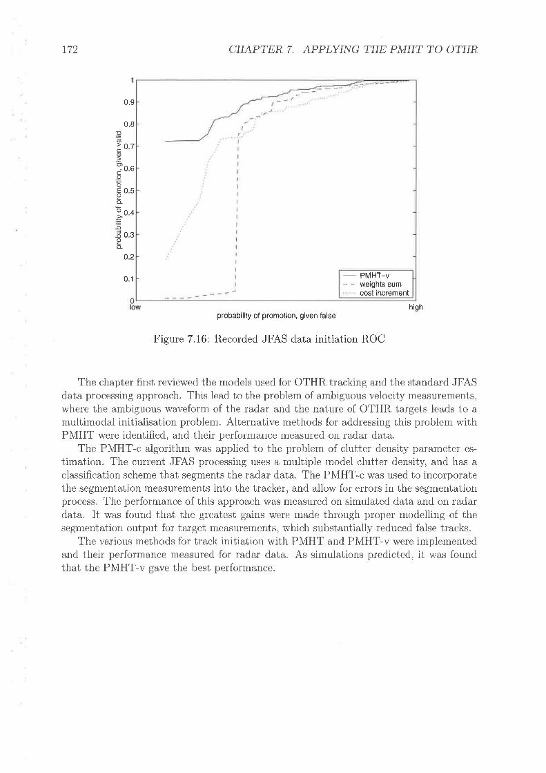
172 CHAPTER 7. APPLYING THE PMHT TO OTHR
0.9
0.8
0.1
highprobability of promotion, given false
Figure 7.16: Recorded JFAS data initiation ROC
The chapter first reviewed the models used for OTHR tracking and the standard JFASdata processing approach. This lead to the problem of ambiguous velocity measurements,where the ambiguous
"¡/aveform of the radar and the nature of OTHR targets leads to a
multimodal initialisation problem. Alternative methods for addressing this problem withPMHT were identified, and their performance measured on radar data.
The PMHT-c algorithm was applied to the problem of clutter density parameter es-timation. The current JFAS processing uses a multiple model clutter density, and has aclassification scheme that segments the radar data. The PMHT-c was used to incorporatethe segmentation measurements into the tracker, and allow for errors in the segmentationprocess. The performance of this approach \Mas measured on simulated data and on radardata. It was found that the greatest gains were made through proper modelling of thesegmentation output for target measurements, which substantially reduced false tracks.
The various methods for track initiation with PMHT and PMHT-v were implementedand their performance measured for radar data. As simulations predicted, it was foundthat the PMHT-v gave the best performance.
o7
06
05
o4
03
o2
E(ú
0)
O)i.EoE
o_
o
=õ(ú-ooo-
_ PMHT_V. weights sumcost increment
Chapter 8
Comparison of the ProbabilisticMulti-Flypothesis Tracker with theProbabilistic Data Association Filter
al-tHE previous chapters demonstrated that the extensions to the PMHT developed inI this thesis provide improved performance oveï the standard algorithm. However, this
is of limited interest if the extended PMHT does not outperform other existing algorithms.In section 1.1, a requirement for an efficient multi-target tracking algorithm for the JFASradar was cited as motivation for pursuing research into PMHT. To address this, thePMHT algorithm that has been developed should be compared with the current JFAStracking algorithm, the Unified PDAF (UPDAF). The PMHT is a multitarget algorithm,and the UPDAF is a single target algorithm. Subsequent research since the installationof the UPDAF at JFAS has produced a Unified Joint PDAF (UJPDAF) [DC01], howeveronly the single target UPDAF is considered. The track initiation scenarios consideredconsist of isolated targets, and multi-target tracking is not required.
In addition to the imperative to justify PMHT research, the comparison of PMHTand PDAF is of interest in itself. Since the PMHT is a recent algorithm, exhaustivestudies have not been performed. In particular, the initiation performance of the PMHThas not been studied, since this thesis and |LSWO1] are the first approaches presented forautomatic initiation. To focus completely on the operational algorithm would give resultspractical, but rather specific. Therefore simulation studies with a simplified UPDAF arealso considered. These simulations provide m.ore general information about the relativeperformance of PMHT and PDAF in track initiation.
This chapter presents a comparison of track initiation with the PMHT and the PDAF.Firstly, the PDAF extensions leading to the UJPDAF are briefly described. Next, anoverview of existing comparisons and higher level considerations is presented. Then thetrack initiation performance is measured via simulations and using recorded JFAS data.The performance of each algorithm will be quantified via the ROC curve for the trackinitiation decision.
8.1 The Probabilistic Data Association FilterThe Probabilistic Data Association Filter (PDAF) [BST75, BSFSE] is an approximationto the optimal recursive Bayesian data association strategy. The PDAF is a single targetalgorithm, so each track is filtered in isolation, and it is assumed that any measurements
773

174 CHAPTER 8. COMPARISO¡ú OF THE PMHT WITH THE PDAF
due to other targets can be lumped into the clutter. The PDAF enforces the singlemeasurement assignment constraint, namely each target track is only allowed to forrn atmost one nÌeasurernent. Since the PDAF is a single target algorithm, each target model,m: My + 1 . . . M, determines independent association probabilities.
The single measurelnent per target constraint means that there o"re rù¡ f 1 assignmenthypotheses for model rn. One for each measurement, and tire hypothesis that no mea-surements are due to the target. Whereas the PMHT derives assignment weights, lDmtrttlre PDAF uses euent probabtli,ti,es. The event probability, 0T(r), is the posterior prob-ability that the rth measurement at scan f is due to target model zn. This probabilityis determined assuming that each measurement is due either to model rn or clutter (thesingle target assumption).
The standard PDAF makes a number of assumptions about the target and clutterbehaviour. The targets are assumed to have linear Gaussian statistics, and all targettracks (i.e. filter models assumed to represent targets) must correspond to valid targets.The clutter is assumed to be uniformly distributed over the surveillance region, and thenumber of measurements due to clutter is assumed to follow a Poisson distribution.
Further background information about the PDAF is presented in Appendix C.
8.1.1 The Unified PDAFThe Multiple Model Unified PDAF (MM-UPDAF) [CD03] is a non-parametric PDAF thatincorporates nearest neighbour validation, multiple non-uniform clutter models, multipletarget dynamic models and target visibility. These PDAF extensions are presented inmore detail in Appendix C. The MM-UPDAF algorithm is used in the operational JFASdetection and tracking software. The term multi,ple model refers to the use of a set ofdynamic models for each target, not to multi-target tracking. These dynamic models canbe used both for ambiguous doppler unwrapping, as described in the previous chapter, andfor manoeuvring target tracking. With M, (known) target dynamic component models,the target model state for model mis æ!e,1or m: Mv + 1...M andp: l...Mr.The event probabilities for target model m àre denoted l3i'(r), with þT'(r) assumed toindependent of Bit(s) if n I m. The MM-UPDAF uses nearest neighbour gating, so thatonly the 1 closest measurements to the predicted target measurement are assumed to havenor-zero association probabilities.
The JFAS system uses a preprocessor that tags each measurement as being caused byclutter component I or2, this is the classification part of the measurement, .(r? e $,2j.This tagging procedure is assumed to be perfect. There are two clutter models, My :2,and the event probabilities for target models m: 3 . . . M are given by
pye|) :prr@ :lti'(r):
bi Pmie (1 - Pdre P'Tr) ,
bi Pmie Pdie#' (":î'¡*7') ";ai c
(k'tr
(8.1)
(8 2)
(s 3)er (.Íî) æç) x;r
Iwhere bi is a normalising constant, ensuring that ! þio(r):t. The term Pmie is
the a priori probability for model componen t e, erVl-rtr. ,n" predicted probability that
8.2, JPDAF COMPARED TA\TH PMHT 175
the target is visible, given data up to the previous scan, Psfp is the probability thatthe target orientated measurement is within the 1 nearest, giy"e¡t rnodel p is the correctmodel, nf is the number of measurements tagged as type c : zìi' fi'om those within the 1nearest for all model components, Nr" is the total number of measurements tagged as type,: .:l) aû, Ai is the spatial area of clutter model c (provided by the preprocessor). The
measurement pdf, *' ("lr'l*T'), is the probability density of the measurement given
that it is due to nlp, but with only an estirnate of the state. This is a normal distributionwith covariance given by the innovation covariance matrix, Sie. Notice that the PDAFuses the innovation covariance to assign measurements, not the measurement variance.This feature was discussed in more detail in chapter 6.
The event probabilities are then used to determine synthetic measurements for eachtarget component model, and a Kalman filter is run for each æle. The derivation of theÌ\,{M-UPDAF event probabilities and state recursions is presented in detail in [Col99].
8.1.2 The Unified Joint PDAFThe MM-UPDAF makes a single target approximation, narnely that the assignment ofmeasurements can be perforrned independently for different target tracks. This assump-tion is invalid when targets are closely spaced with respect to the sensor resolution. Thiscircumstance may also arise in OTHR when multiple propagation paths are closely spaced.In order to improve the tracking performance of the MM-UPDAF, this single target as-
sumption was relaxed and a Multiple Model Unified Joint PDAF was developed [DC01].The event probabilities for this filter are found using substantially more complicatedexpressions than those above, and are not presented here. Since the track initiation com-parison uses only isolated targets, multi-target tracking is not required, and for simplicitythe UJPDAF is not used.
8.2 JPDAF compared with PMHTThe PMHT solves th.e tracking problem using an approach different from that used bystandard tracking algorithms. This results in an elegant algorithm for multitarget track-ing. However, this elegance is not a particularly compelling reason for choosing it overmore established tracking approaches. It is important to compare the PMHT with stan-dard algorithms, to see if practical advantage can be gained through its use. Rather thancompare PMHT with all of the tracking pantheon, this work focusses on the PDAF, sincethis algorithm is widely used, and because it is used in the JFAS radar, data from whichwill be used to provide a realistic evaluation of algorithmic performance. Since the PMHTis by nature a multitarget algorithm, it is sensible to compare it with the JPDAF, or touse single target scenarios. The latter has been chosen because the comparison focusseson track initiation. Multitarget scenarios would unnecessarily complicate the initiationanalysis and the results would most likely depend on the particular scenario chosen.
8.2.1 Philosophical DifferencesThe fundamental philosophical differences between PMHT and JPDAF were discussed inthe original presentation of the PMHT [SL95]. When the batch length is one, the PMHTbecomes a recursive filter and the two appear superficially similar. Both algorithms canbe implemented using probabilistic weights to form synthetic measurements that feed

776 CHAPTER 8. COMPARISO¡ú OF THE PMHT WITH THE PDAF
a Kalman Filter for state estimation. However, the PDAF association probabilities arebased on the predicted state, which is a deterministic function of the state estimate at theprevious scan. In contrast, the PMHT uses the ML estimate of the current state. [SL95]cites this as a source of bias in the JPDAF.
The JPDAF updates the state with each measurement and then cornbines the stateestimates into a single estimate. The PMHT combines the measurements to form syntheticmeasurements which are then smoothed.
The JPDAF assumes a one to one assignment of measurements to targets (providedthat all targets are detected). The PMHT assumes that each measurement is assignedindependently. This effectively means that the PMHT allows the event that more thanone measurement is caused by a particular target. The effect of this depends on thevalidity of these assumptions for the particular data set.
The covariances calculated by the JPDAF reflect the current uncertainty in the stateestimate, whereas those computed by the PMHT are not statistically defined in this man-ner. [SL95] provides a discussion of the interpretation of the PMHT covariance matrices.
8.2.2 Practical Differences
The rnost obvious differences between the algorithms can be broadly described as imple-mentation issues. The PMHT is a very simple algorithm to implement because of theindependence of the assignrnents. This independence results in an algorithrn with cornpu-tation requirements linearly scaling with the problem size, and which can be implernentedin a massively parallel manner. In contrast the JPDAF must deal with an event spacewhose dimension grows combinatorially with the problem size (the number of targets andmeasurements within each scan). This combinatorial growth makes the JPDAF a greedyalgorithm and the efficient implementation of the JPDAF is an area of research in itself(for example, [ZB95r, DC01]). A further issue, besides speed, is the memory required tostore the joint event probabilities. In a naive implementation, all the events would beenumerated and their probabilities stored for updating tracks. For challenging scenarios,when multiple dynamic models are used, the number of the joint events can make storingall their probabilities impractical (requiring gigabytes of rnemory).
A more subtle difference is that the PMHT associates measurements using the targetmeasurement covariance, whereas the JPDAF uses the innovation covariance (which isthe expected scatter of the target measurement given the current state estimate and itscovariance). This means that the JPDAF gives higher probability to distant measurementsthan the PMHT does. Also, it gives the JPDAF an ability to dynamically inflate theassociation process if a track starts to diverge from the true target trajectory. Thisimpacts on the PMHT's ability to handle manoeuvres and heavy clutter.
The algorithms also vary significantly when multiple measurerlents are sufficientlyclose to be given high assignment weights. In the JPDAF, this causes the covariance ofthe state estimate to increase, reflecting the uncertainty about which measurement is thetrue target measurement (recall that the JPDAF assumes that there can only be one truetarget measurement). This occurs through the measurement scatter term in (C 7) In thePMHT, each of the measurements is assigned with high probability to the target model.Since there are more measurements of the target, the covariance is reducerl. This happensbecause the sum of the weights for this model is greater than unity and so R reflects amore accurate measurement than R (namely lRl < lRl).

8.3. TRACK INITIATION O¡\r SIMULATED DATA 777
8.2.3 trxisting Comparison StudiesThe existing comparisons of PMHT arid (J)PDAF have been mainly orientated at theanalysis of steady state tracking performance. The emphasis has been on what Ruan andWillett call "the game of lost-tracks". Namely, given established tracks, what is the prob-ability that the algorithm will maintain the track over a series of scans. In both [RWS95a,]and [RW01a], the PMHT algorithm is demonstrated to show sinilar performance to theJPDAF under easy conditions, but superior performance under difficult conditions.
In lR\\iS99], the Cramer Rao lower bounds for estimator variance are examined forthe PMHT and PDAF measurement models. These models differ due to the differentassumptions made about the assignment of measurements. This work showed that thebound for the PMHT is higher than the PDAF. This indicates that a minimum varianceunbiased estimator for the PDAF measurement model would have a lower variance thana minimum variance unbiased estimator for the PMHT. Unfortunately, this result doeslittle to illuminate the performance of the PMHT and PDAF algorithms.
8.3 TYack Initiation on Simulated DataIn chapter 6, sinulated experiments were used to examine the track initiation perfor-nrance of the PMHT using various initiation schemes. Of these competing approaches,the PMHT-v was found to give the best overall performance. As described earlier inchapter 6, the visibility model, which is a special case of the hysteresis assignment model,is analogous to the nodel used by the UPDAF for track quality decisions.
The initiation simulations in chapter 6 are now repeated with a simplified versionof the UPDAF algorithm. This simplified algorithm needs not deal with multiple cluttercomponents or target dynamic models. The performance of the UPDAF is compared withthe PMHT-v performance. Two versions of the PMHT-v are used: the standard batchprocessor, and a time recursive algorithm. Intuition suggests that batch processing willprovide an advantage to performance. Since the UPDAF is a time recursive algorithm,it may seem a little unfair to compare it with a batch approach. Howevet, for the trackinitiation process, a real time estimate of candidate tracks is not provided to the user.Instead, the candidate is hidden until it passes the promotion test. This means that batchprocessing could be used for track initiation, even in a system requiring immediate targetstate estimates for each scan. Both the recursive and batch versions of the PMHT-v areretained to demonstrate the benefit gained by using batch processing.
Three different clutter distributions were considered in chapter 6; uniform clutter, chi-squared clutter, and polynomial clutter. ROC curves for these clutter distributions areshown in figures 8.1, 8.2, and 8.3 respectively. These figures show the high false detectionrate clutter examples from chapter 6. Low false detection rate examples are not shownbecause they give results simiiar to the high rate, but with reduced differences betweenthe curves.
An interesting feature of the ROC curves is that sometimes the recursive PMHT-v givesa higher probability for promoting valid tracks than the batch P\4HT-v for a particularprobability of promoting false tracks. This occurs because the ROC is a normalisedpicture. The recursive PMHT-v has a much higher rate of divergent candidates than thebatch PMHT-v (see the following section). The tracks which diverge in the recursivePMH-T-v are invariably those which are assigned a low probability of being visible by thebatch PMHT-v. This means that the average quality of tracks in the PMHT-v is reduced,and the ROC is therefore effected.

178 CHAPTER 8. COMPARISO¡\r OF rHt, PMHT WITH THE PDAF
7
06
05
40
03
02
põoo)c.9oEoo-oÈb(ú-ooo_
0.9
0.1
0 t-110- 10'probability of promotion, given false
Figure 8.1: Uniform Clutter, high density
D110- 10'probability of promotion, given false
10010
0.9
I0
07
06
05
0
0
põcoo)i.9oEIo_
o.=õ(ú-ooo_
4
3
o2
- PMHT-v, batch
- - PMHT-v, recursiveUPDAF
- PMHT-v, batch
- - PMHT-v, recursiveUPDAF
01
Figure 8.2: Chi-Squared Clutter, high density
100

8.3. TRACK INITIATIO¡ú O¡\I SIMULATED DATA 179
0.1
,t _110 - 10
probability of promotion, given false100
Figure 8.3: Polynomial Clutter, high density
On the uniformly distributed clutter, all give similar performance, except for verylow probability of promoting a false track, where the recursive PMHT-v drops off. Forchi-squared distributed clutter, recursive PMHT-v and UPDAF give simiiar performance,with batch PMHT-v significantly better. For the polynomial distributed clutter, thePMHT-v batch is slightly better than the recursive version, and the UPDAF gives verypoor performance. The UPDAF fails in this last case because of the high concentrationof false detections at low measurement values. Although the distribution itself is non-physical, the primary difficulty in OTHR radar data (for initiation at least) is highlyconcentrated false detections due to phenomenon such as range folder clutter.
Overall, the batch PMHT-v is clearly the best track initiation approach in these sim-ulated examples.
8.3.1 Initialisation Robustness
Table 8.1 lists the number of divergent trials for each of the scenarios. As a general rule,the batch PMHT-v gives a much lower rate of divergent tracks. The recursive PMHT-vand the UPDAF give similar results, with the recursive PMHT-v slightly worse. Therecursive PMHT-v does particularly poorly in the high false alarm rate, uniform clutterexample. These results serve to highlight the advantage of using batch processing, whichis not a viable option with the UPDAF. The similarity between the recursive PMHT-v and the UPDAF results indicates that the innovation homothetic model has done anacceptable job of making the PMHT robust to initialisation errors.
0.9
0.8põ> 0.7c(1)
? o.oc.9oE 0.5oo_
9 o.¿ð=õ(ú ^^-o U..t
o20
- PMHT-v, batch
- - PMHT-v, recursiveUPDAF

180
clutter typefalse alarm rate
batch PMHTrecursive PMHT
UPDAF
highchi-squared
low high
619 2346 292 5631655 3460 975 15741336 25rr 850 1238
CHAPTER L COMPARISO¡\¡ OF THE PMHT WITH THE PDAF
uniform polynomiallow low
340TI77r077
90119991700
Table 8.1: Number of divergent trials
8.4 Track Initiation on JFAS DataAs with the earlier track initiation analysis, JFAS data is now used to support the simula-tion findings. The UPDAF algorithm is the current tracking algorithm for the JFAS radar.This algorithrn reports a track quality measure referred to as track confidence which isderived from the posterior visibility probability. To produce empirical ROC curves, theconfidence of candidate tracks is reported after a fixed number of scans. This is the sameas the batch length used for the PMHT algorithm, namely 8 scans.
The ROC curve derived for the JFAS UPDAF tracker is shown in figure 8.4 withPMHT-v curves for batch and recursive processing. In chapter 7, a number of differentapproaches for modelling clutter were tested. The PMHT-v curve in 8.4 is derived usingthe degenerate PMHT-c filter which assumes that the clutter classiflcation iuformationis perfect. This is the same philosophy as that adopted by the UPDAF, so it should beused for a fair comparison.
It can be seen that the PMHT-v performance is superior, particularly when the falsetrack promotion probability is low. The recursive PMHT-v algorithm gives worse perfor-mance than the batch PMHT-v. The UPDAF shows a sudden drop off in perforrnance,resulting in an effective minimum false track promotion probability below which detectionis impossible, This occurs because the track quality measure for the UPDAF is boundedbetween 0 and 100. To achieve very low false track rates, the promotion threshold must beincreased until it becomes very close to 100 where all tracks are rejected. In essence thismeans that some false tracks can never be suppressed with UPDAF. The sharpness of thetransition occurs because most of the UPDAF tracks formed on strong targets have thesame (or very similar) confidence values. In contrast, the PMHT-v is able to suppress allof the false candidate tracks and still promote a high proportion of the valid candidates.
8.4.1 Initialisation RobustnessIn each of the initiation comparisons performed in earlier parts of this thesis, the analysishas included ROC curves and tables of initialisation robustness. The initialisation robust-ness has been quantified by a count of the number of times a candidate that was i,ni,ti,ali,sedon a ualtd detecti,on diverged from the true target trajectory. To analyse this quantity forreal data, would require accurate knowledge of whether each target was detected or notfor each scan. Acquiring this knowledge would be very time consuming, and it has notbeen done. Consequently, the initialisation robustness on real data is not considered.
8.5 Established Track PerformanceThe focus of the work in this thesis has been track initiation. However, this is only oneaspect of tracking performance. There is also a raft of tracking performance metrics that

8.6. SUMMARY 181
highprobability of promotion, given false
Figure 8.4: ROC curves for JFAS data
can be proposed for established track performance. For example, [CDD96] lists numerousmetrics which include track initiation performance as well as estimation accuracy andmultitarget correctness measures. Consideration of these is beyond the scope of thisthesis, as is any further PNIHT development that may be required to address applicationspecific problems in established tracking.
8.6 SummaryThis chapter has presented a comparison of the track initiation performance of the PMHT-v and UPDAF algorithms. The UPDAF is the algorithm currently used for tracking in theJFAS radar. The PMHT-v was implemented in both batch and time recursive forms. Fora variety of simulated clutter conditions, the batch PMHT-v was found to give better trackinitiation performance than the UPDAF, and to recover better from poor initialisationwhen the innovation homothetic initialisation scheme was used. The recursive PMHT-vgave comparable performance to the UPDAF, except in one example where the UPDAFperformed very poorly.
These algorithms were also compared using JFAS radar data. In this case, the UPDAFused was the operational radar tracking algorithm, a result of considerable research ef-fort. The track initiation performance of the PMHT-v was found to be superior in bothrecursive and batch fotms, with the batch PMHT-v giving the best results.
0.9
0.8põ> o.7Cq)
?o.oc.o
E 0.5oLo.¿=o3 o.soo_
0.2
0.1 - PMHT-v batchPMHT-v recursiveUPDAF

182 CHAPTER 8. COMPARISO¡\I OF THE PI,IHT WITH THE PDAF
Chapter ISummary
rftHIS thesis has introduced a number of enhancements to the PMHT algorithm, mo-I tivated bv the Over the Horizon Radar tracking problem. The primary two en-
hancements are the incorporation of classification information, and the introduction ofa discrete state model for the assignment prior probability. The modified PMHT algo-rithms achieved through these enhancements are referred to as PMHT-c and PMHT-yrespectively.
The benefit of the PMHT-c and PMHT-y algorithms has been demonstrated throughsimulation studies, and through the application of both to recorded OTHR data.
9.1 Classification MeasurementsThe standard PMHT algorithm deals with measurements that are observations of thestate of a particular model. The algorithm provides state estimates by determining theprobability of an assignment index that links measurements with the model that causedthem. The PMHT-c is an extension of the PMHT that deals with the more generalproblem where the tracker is also provided with measurements of the assignment indexitself. These measurements are classifications, and are assumed to be independent ofthe model state, and hence the normal measurements. The PMHT-c simplifies to thestandard PMHT if the classification measurements are uninformative.
The PMHT-c algorithm has been shown to improve state estimation accuracy, andmanoeuvre tracking, by using extra measurement information to increase the probabilityof the true assignment index. The probability mass function of the classification mea-surements can be represented as a matrix and is referred to as the conf'usion matrix. ThePMHT-c was derived under the two conditions of known and unknown confusion matrix.Simulations demonstrated that the PMHT-c is not sensitive to the confusion matrix val-ues if it is assumed to be known. Further, in the experiments conducted, it was seen tobe advantageous to assume an artificially high probability of correct classifications.
9.2 Dynamic Assignmcnt PriorThe second extension to the PMHT algorithm was the addition of a discrete Markovprocess as an underlying dynamic model for the assignment prior probability. Under thestandard PMHT model, the assignments are independent identically distributed randomvariables drawn from a possibly unknown prior probability mass. If this mass is unknown,the PMHT allows for its estimation, but only under the restrictive assumption that it is
183

184 CHAPTER 9. SUMMARY
either independent between scans) or identical. This assumption was relaxed by intro-ducing a state model for the assignment prior, referred to as the hysteresis model. Theonly restriction on the assignment state rnodel was that the state was required to be adiscrete random variable. This restriction was imposed to enable the optimal solution ofthe estimation of the assignment state, or its probability. A continuous assignmeut statecould be used, but this would require an approximate solution method, such as particlefiltering or a Taylor Series analytic approximation. This thesis dealt with the situationwhere the statistics of the assignment state are known, however methods were identifiedfor the case where these statistic are unknown.
Two algorithms were derived under this geueralised assignment model: the PMHT-ymwas derived by treating the assignrnent state as missing data. The resulting algorithmcalculates the probability mass of the assignment state, similar to the way the standardPMHT calculates the assignment probability rnass. The PMHT-y- algorithm can beimplemented using an iterative scheme alternating between a bank of parallel KalmanSmoothers for rnodel state estimation, and a joint Hidden Markov Model Smoother todetermine the probability of the assignment state.
The PMHT-ye was derived by treating the assignment state as a quantity to be es-
timated. This means that the assignment state is treated as an extension of the targetmodel states, and is iteratively estimated along with the target dynamic states. In thiscase, the assignment state is estimated using a joint Viterbi algorithm, run in parallelwith the Kalman Smoother bank for dynamic state estirnation.
Each of the algorithms derived under the Hysteresis model requires joint target modelprocessing for part of the algorithm. This is a result of the normalisation across modelsin the assignment prior and can only be avoided through making approximations. Thismeans that both the PMHT-ym and PMHT-ye contain steps with exponential complexityin the number of targets.
Simulations were used to demonstrate how both the PMHT-ym and PMHT-ye algo-rithms were able to give much better estirnation accuracy for the assignment prior whenthe prior was smoothly varying with time. This improvement was observed to be a resultof the Hysteresis model allowing the PMHT to incorporate data from adjacent scans toestimate the assignment prior.
9.3 Track InitiationThe problem of track initiation was addressed for PMHT: under the standard PMHTassumptions, the number of models is fixed and known, and prior information is availablefor the models. This is rarely the case in practice. An approach for initialisation based onthe homothetic measurement model was introduced and demonstrated to greatly improvethe robustness of PMHT to assumptions about the state prior. A dynamic number oftarget models was achieved by introducing methods for automatic track initiation. Thiswas achieved by over modelling the system using a number of candidate models, and dis-carding redundant candidate models based on a significance test. Different test statisticswere considered, including those based on intuition, Model Order Estirnation, and theapplication of the Hysteresis model.
It was shown that the ui,si,bi,li,ty model used for track initiation with PDAF and othertracking algorithms \Mas a special case of the Hysteresis model where the assignment stateis assumed to be binary. The PMHT-y- algorithm incorporating visibility was referredto as the PMHT-v.

9.4. RADAR DATA PERFORMANCE 185
Simulations were used to investigate the perforrnance of the proposed initiation meth-ods on a variety of clutter conditions. It was found that the PMHT-v algorithm gave thebest overall initiation perforrnance, and gave particular advantage when the probabilitydensity function of the clutter was non-uuiform.
9.4 Radar Data Performance
In order to verify the simulation results, and because of a perceived need for a truemultitarget tracking algorithm for OTHR, the PIVIHT and the enhancements above wereimplemented for data from the JFAS radar. This implementation required the tracker toalso address a number of practical problems with the JFAS data. The two main issueswere the JFAS clutter modelling approach and the problem of unwrapping ambiguousdoppler measurements.
Several approaches were identified for addressing the doppler unwrapping problem.These included modelling the true doppler frequency as an unknown track parameter,treating it as missing data in an EM context, and using a non-physical mixture modelwhich modelled the target as a superposition of all possible unwrapped dopplers. It wasfound that the unknown parameter approach gave the best results.
The clutter modelling problem was addressed by applying the PMHT-c to the JFASdata. The JFAS pre-track processing produces feature information which is used in aclassifier to segment the measurements into different classes. The PMHT-c was usedto incorporate this classification information, and to allow for classification errors. Analternative approach whereby the tracker was given direct access to the feature informationwas also identified. These approaches r,Ã/ere tested using simulated data and using recordedJFAS data. It was found that the best performance was obtained by removing the classifierand giving the tracker direct access to the feature measurements.
The proposed track initiation approaches were applied to recorded JFAS data andthe performance of each observed. As with the sirnulated results, it was found that thePMHT-v, which is a special case of the Hysteresis dynamic assignment model, gave thebest performance.
9.5 Comparison with PDAF
The enhancements made to the PMHT enabled it to deal with a broader range of dataconditions. However, the problems solved by the new PMHT variants have already beenaddressed using other tracking algorithms. In order to gauge the usefulness of these newvariants, the PMHT performance was compared with that of the Unified PDAF, thealgorithm currently used for tracking with the JFAS radar. Track initiation performancewas compared based on sirnulated data and on recorded radar data. It was found thatthe PMHT-v algorithln gave better performance than the UPDAF.

186 CHAPTER 9. SUMMARY
9.6 Future 'Work
As with any research, this thesis leaves areas which might be explored by future work
9.6.1 Classification InformationAn early assumption in the PMHT-c formulation is that the classification measuretnentsare independent of the state, and the state measurements. This assumption may notalways be valid. In some applications, the classifier output may be dependent on thestate. For example, a ship classifier may use a length estimate as a feature. The accuracyof the estimate, and hence the classification accuracy, would be dependent on the ship'saspect angle and range. These are components of the dynamic state. It is reasonablystraightforward to use a state dependent confusion matrix for measurement association,however under this circumstance, the classification measurement provides state informa-tion. The proper incorporation of this information in the state optimisation requiresfurther investigation.
The analysis of the PMHT-c in this thesis has considered how a classifier can be used toenhance state estimation. The complementary problem is the influence of state estimateson the classifier output. Further, the classifier and tracker could be tightly coupled, suchas in lCP01] to improve both by cross fertilisation.
9.6.2 Prior Dynamics
The Hysteresis model presented in this thesis was solved under the assumption of a discreteassignment state. This rnight be viewed as an approximation to a continuous assignmentstate, using a fixed grid method. Alternative methods could be used, such as particlefiltering.
An obvious shortcoming of the PMHT-ve and PMHT-vm algorithms is that bothhave exponential complexity in the number of targets. This is disappointing, since oneof the advantages of the standard PMHT over other tracking approaches is its linearcomputational growth. The exponential cornplexity is an inevitable result of the modelcoupling which occurs due to normalisation of the prior. However, with further tesearch,it may be possible to achieve similar performance with an approximate algorithm thathas reduced complexity.
9.6.3 TYack Initiation and InitialisationThe Innovation Homothetic Model presented in this thesis is an ad hoc approach fortackling the PMHT initialisation problem. In its use, no consideration was given to issuessuch as convergence. There are many other methods that might be used, and initialisationremains an open question for PMHT.
While the track initiation research presented in this thesis was underway, other par-allel work on initiation with PMHT was done using a Hough Transform based approach[LSW01]. Future comparisons need to be performed to ascertain the relative merits ofthis approach compared with PMHT-v.

e.7. co¡úcLusro¡üs 187
9.6.4 OTHR ImplementationThe prototype OTHR algorithm developed in this thesis has been demonstrated to givegood performance for track initiation. Howevet, there are numerous other aspects oftracking which need to be addressed before the algorithm would be appropriate for oper-ational evaluation. There are many problems in established tracking which have alreadybeen addressed with the UPDAF, and some of these solutions may be incorporated intothe PMHT algorithm.
9.6.5 PMHT and PDAF ComparisonThe comparison of PMHT and PDAF presented in this thesis considered only the problernof track initiation. \Mhiie other studies have cornpared aspects of established track per-formance, an overall comparison between the two algorithms would be of interest. Thisis especially true of the recorded radar data comparison.
Through the implementation of the JFAS mixture model for clutter, evidence has beenfound that the PMHT is less sensitive to the assumed density functions than PDAF. Ifthis is the case, it is an important fundamental property of the algorithms, and could befurther investigated through simulation studies.
9.7 ConclusionsThis thesis has presented new extensions to the Probabilistic Multi-Hypothesis Tracker,motivated by the Over the Horizon Radar tracking problem. Some of the research hasprovided solutions to application focused problems, such as track initiation and cluttermodelling. Other work has given rise to fundamental generalisations of the PMHT algo-rithm to allow it to properly deal with a wider range of measurement processes.

188 CHAPTER 9. SUMMARY

Appendix A
Innovation Homothetic Model forInitialisation Robustness
rftHrs appendix presents details of the initialisation approach introduced in chapter 6,
I which uses the innovation covariance matrix as a homothetic measurement pdf. Theuse of the innovation covariance matrix aliows the second homothetic model to effectivelyexpand its assignment gate when the state initialisation is poor.
The Homothetic PMHT presented in [RWS95a] makes use of a scaled measurementcovariance matrix for the homothetic model. This has the convenience that the covarianceof the mixture components for each target model are simply scalar multiples of each other.The result is that the EM auxiliary function is maximised by a Kahnan filter that uses themeasurement covariance modified by a scalar factor. In general, the innovation covariancewill not be a scalar multiple of the measurement covariance since it also includes thecovariance of the current state estimate. Recall that the innovation covariance is given by
sT : HTPT*ÏT' + RI (A 1)
When the innovation covariance is used as a second homothetic measurement model,the resulting solution will not be a Kalman smoother using a scalar multiple of the mea-surement covariance.
The solution for the homothetic measurement model where the second component ofthe mixture density has an arbitrary covariance matrix now follows. Assume that thetwo mixture components are not equal components of the mixture, but that they haveunknown mixing proportions which may be a function of time. This is a generalisation ofthe homothetic mixture model first used in [RWS95a]. The extension of the homotheticmodel to use arbitrary covariance matrices is known [Str00a, Lug01], but has not beenpublished. Having derived this PMHT, the extension to a mixture of more than twoarbitrary covariance components will be obvious.
The missing data are the assignment indices K. As introduced in section (3.5.1),the homothetic mixture model uses two index lists. For measurement z¡r, the index kftakes a value in the range L .. A,t and indicates the model that caused the measurement.The inclex kl,, takes either the va,lue 1 or 2, indicating the component of the homotheticmixture for model kl, that caused the measurement. So,
p ("r,lxr,kl,kî) : ekl''nï' (.*l*f'") (A 2)
where the mixture compone nts ç!l''n?' are Gaussian distributions given by
eit Qr,l*T) N .n/ (H¿æi, Ri)
189
(A 3)

190 APPENDIX A. I¡ú¡úOVAT/ON HOMOTHETIC MODEL
ei'Q*l*T) N N(H¿æi,Si) (A 4)
For each target at each scan, introduce the mixing proportions pTp so that the priorprobability mass of the indices is given by
P(kl,-m) :P (ki: plk'* - m) :
(A 5)
(A 6)
The mixing proportions are constrainedby pTt + pT2:1and for each clutter modelPTr : I'
Also define temporal sets as follows
p, : lp\r, pl', p?',. . . py'l (A 7)
andp = lpt, Pz,. . . , Prl (A 8)
Since the observer and measurement model have been modified, the complete datalikelihood is modified. The conditional probability of the received measurements is givenby
P (zlK,X) : (A.e)
The probability of the assignments is given by
-TItttTNDPt'
il fi ekt.n?. (r* *fl.)t:7 r:l
TntP (K) : fl flrfi" or;Ln\'
z*læ
(A.10)
(A.11)
t:l r:7Thus the new complete data likelihood is given by
L(oMil
m:L
,z):
{rrønyw@?-r)}IIul"fi. ,frn?. ç!Ln?.r:7
kl,
The conditional probability of the assignments is also modified. There are now twoweights for each track and mea"surement because of the two mixture components in thetarget measurement density. The new conditional probability of the assignments is thus
P(KIX,Z): Ie2rrtr (A.12)
where the weight uk!,k!,tr is given by
irkl, pkLk?, ek ,rr, ("rrl*f|)
T rlt
llll.*;t:l r:1
wkl,r<l,tr : M2
t I nT pT'oe?'o (.*l*T)m:I p:I
(A.13)

A.1. MAXIMISATIO¡\I STEP
Equations (4.11) and (4.12) are no'ù/ substituted into auxiliary function to obtain
(A.14)
, px(o(x,ntK
TK
tK
tK
i),IJ(¿) , p(i)) :
{,"*u, @i) +å.- ,þi @T -*t\} H ,t!.r7.,+
nt .ì T nL
Iro* "!t. | ilf|,'l!"u7,,,+r=t ) l:tr:t
t -\nTr
191
(A 1e)
lvItm:1
TtTt
t:lTt
t:l
nt
(,,. *f*(ù) )ú fr.,t1,.*,.n
I to* prl'rT ,t1,,*?,*ir:7nt
Dto* çkl'k?'r:1
where the dependence on 1¡" .(r-r) terms is implicit in the weight ,llii',*.In a similar way as for the standard PMHT, rewrite (4.1a) as
T T Iv'T
I (x,rr, plx(';), fr(i), p(i)) : Ðqy + t etn tD,Ð,qA (4.1b)m:7 t:I t:l m:7
The Qp term in (4.15) depends only on the target model states and the rneasurementsand is given by
TTnt2
Q'i : ros,þto @Ð + I to* ,þT @Tl*7,) * I t t roeefo Q*l*T).|),* (4.16)t:I t:l r:I p:I
The Q¡n term in (4.15) depends only on the prior probability fI and is given by
ntMQ,n : t t rosr! (,f1,, *,Í3*) (4.17)
r:I k:IThe Qfr term in (4.15) depends only on the prior probability p and is given by
/-\ttL -
nt 2
,{tp=ttrogpiewfor, (4.1s)y:! p:l
4.1 Maximisation StepSince it is the simplest, start by maximising the Qtn term in (4.15). Notice that theexpression for Q¿n is almost the same as that found for the standard PMHT whose solutioni. gi,r"n in (S.Si). By substituting .fl*+rf;)r,tot rf;),r" (3.51), the estimate for fi atiteration z is given by
k1Tt D,lll,, +,tL,(i+1)
- 1
nt
r:lTL¿
The Qfi term in (4.15) is maximised in a similar way to l,he Q¡n term. Qfi is tobe maximised subject to the constraint pT' + pT2 : I. This is achieved by using theLagrangian
Lo(^,f) : tlto* pTrf)r*+\k,,nt2
r:1 p:I
2
k:r(A 20)

L92 APPENDIX A. I¡\r¡\IOVATION HOMOTHETIC MODEL
where \fr,, is the Lagrange multiplier.Differentiating the Lagrangian with respect to pT' and solving for stationary points
gives
-mp(if-l\ 1Pt :\p
,rm,t L*9,*r:1
(A.21)
(^.22)
(A.23)
Reapplying the constraint gives
-mp(i+1)Pt:
Àfn,t: tt r9o,,nt2
r:1 p:l
So the estimate for pie at iteration z is given by the unique stationary point of theLagrangian
nttr:I
(?)mptru
t (.f;,:) *,fl,*)nt
r:I
The estimate of pie is thus the proportion of weights for that measurement model atscan f
^.2 Target State Maximisation
A modified Kalman filter algorithm is now derived for the target state update followingthe approach used in [SL95].
Recall that (A.a) defines (fll and ({" u"
ei'Q*l*T)eT'Q*l*T)
- ,n/ (H¿æi, R¿)
- N (H¿æi, S¿)
and that (,d.16) gives Qp as
T
QT :Ios,þ'o@Ð + I to* ,þT @Tl*7') + I t t Ioeefo Qnl*T) rflo,,Tnt2
t:7 r:L p:l
Consider the measurement dependent part of QT uf scan ú, namely
nt2
t t los (o (z,læ) up,r:I p:L
where the scan index ú, the model index m and the iteration index ø are suppressed forsimplicity of notation.
Substituting the (e definitions from (4.4) write
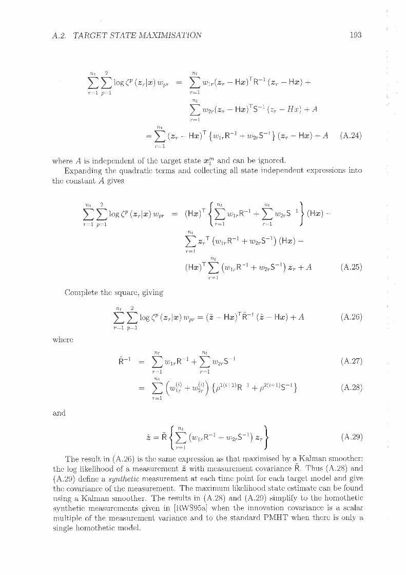
A.2, TARGET STATE MAXIMISATIO¡\T 193
(A.27)
(A.28)
(A.2e)
t t ros (' (z,lr) we, D.r,(t, - Hæ)rR-t (r, - Hæ) +nt2
r:I p:L
nt
r:Int
D.r,(., - Hø)r5-t Q, - Hr) + Ar:l
: t (", - Hn)r {wyR-l + wz,S-r} (t, - Hæ) + A (^.24)nt
r:I
nt
(Hr).
nt
r:1
nt
where A is independent of the target state n! and can be ignored.Expanding the quadratic terms and collecting all state independeut expressions into
the constant A gives
t t log (o (z,læ) we, Irr"R-t+Dwz,S-7 (H') -nt2
r:l p:l
nt
r:I
nt
r:l
D",'(tur"R-l *,u2"S-1) (Hr) -nt
(Hr)tI (rr,*-1 +w2,S-r) ",+ I (4.25)r:l
Complete the square, giving
t t los (o (rÀ*) up, : (2 - Hn)r R-t (2 - Hæ) + A (A.26)nt2
r:l p:Iwhere
and
R-1 Drr"R-t+twz,S-rr:l r:l
i(rl:) *-y)) {p1(z+r)R-l + p2(¿+1)s-1}r:I
nt
2:R I (tr;t"n-r + w2,S-1) z,r:1
The result in (4.26) is the same expression as that maximised by a Kalman smoother:the log likelihood of a measurement 2 wilh measurement covariance R. Thus (4.28) and(4.29) define a synthetr,c measurement at each time point for each target model and givethe covariance of the measurement. The maximum likelihood state estimate can be foundusing a Kalman smoother. The results in (4.2S) and (A.29) simplify to the homotheticsynthetic measurements given in [RWS95a] when the innovation covariance is a scalarmultiple of the measurement variance and to the standard PMHT when there is only a
single homothetic model,

194 APPENDIX A. I¡ü¡üOYA?ION HOMOTHETIC MODEL

Appendix B
Fbll Radar Algorithm
Chapters 4, 5 and 6 provided a number of theoretical advancements of the PMHT algo-rithm, and chapter 7 presented solutions to particular OTHR data issues. All of thesealgorithmic extensions have been presented in isolation. Realistically, it is desirable toincorporate many of these advances into a single algorithm for the radar data. The deriva-tion of such an algorithm is essentially a matter of careful notational accounting and isnot presented here. This is because of the amenable structure of the PMHT framework.Instead, an example of one of the algorithms run on radar data is presented.
This algorithm incorporates:
o the PMHT-c approach for clutter parameterisation with estimated classifier confu-sion matrix
o the innovation homothetic model for initialisation
o the PMHT-v approach for track initiation
o the mixture approach for ambiguous velocity resolution
8.1 Statement of Algorithm1. The first step with all PMHT variants is initialisation. There are several different
variables that need to be initialised for this algorithm.
(a) Clutter model states, X1(0) and X2(0): mean of amplitude distribution
(b) Clutter mixing proportionr, of(o) : 0'5
(c) Classifier veracity, tfo) ut d "lo)
(d) Target model states, X3(0),. .. ¡nz(o)
(e) Target model visibilities ' P(d'T:1;(o):0'11 for all m.
(f) Target homothetic measrüement component mixing proportion", pT'@) : 0.5for all target models m, for all scans ú and all dynamic components, p.
(g) Target dynamic component mixing proportions, Pr^(P) - M;t
2. Calculate the assignment weights for each model (component model) and measure-ment. The expressions for target model weights and clutter model weights are differ-ent because the target models are substantially more sophisticated than the clutter
195

196 APPE,NDIX B, FULL RADAR ALGORITHM
models. Lel ú denote a pre-normalised assignment weight. The pre-norrnalisedassignment weights are given by
(a) For clutter model nù € Lr2 and measurement z¡,
o (r,,1*7"')o!þ)
",,;, ^eî (zr,p7ro)
,mk(i) prm{o) @)p ("*l*Trr,r)
,mk(i) p rm(i) (ç) c,r,> ^Çr (t *l*T"o')
P(DrlX,Z):ffi
Umtr
MNIr2
(8.1)
(8.2)
(8.3)
(b) For homothetic measurement component k of dynamic component p of targetmodel m € 3,... M and measurement z¡,
ú)^tu(k,p)
at(Dr): I
PdTL¿
PdTÙ¡
3. Calculate the visibility probabilities for each target model using the HMM smoother
Dt-t {F_", (aTl¿T,)} o r"lot,xt) ,-t-t(D,-,) (B 4)
þr(Dr): I fI rä, (d,T*,ld,T) P (Zr*rlDr+r,X,+r) 0r+r(Dr*r) (B 5)M1¡
Dt+t
nt
P (ZtlDüX) : n'Qr,lDr,Xr)
m: 1
r:7
Dt
r - Pd DrDr'TL¿
(wu, + {uzt,) t I I Ð oT*^r,(k, p)
The weights are then normalised according to
a:$ p:l þ:!(B 6)
if m:7,2 (8.7)| - Pd DrDr.
rL¡umtr :\e (Dlx,z)P (.r,lDt,Xt)
wmff
u^t,(k,p) : t P (Dtlx,z1 Ë-aß-' e)
Dt \- ¿r--) -' P (t"lD"X') m:3,...M (88)
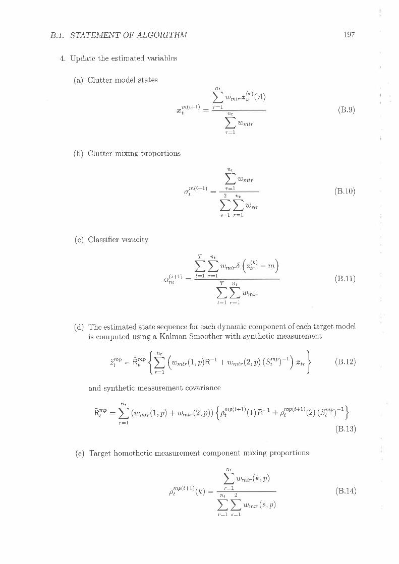
8.1. STATEMENT OF ALGORITHM
4. Update the estimated variables
(a) Clutter model states
D,^,,
197
(B.e)
(8.10)
(8 11)
(8.13)
nt
i+1) _ r:1| .^r,"Í? çq)
rn(nt' nt
r:l
(b) Clutter mixing proportions
(c) Classifier veracity
*l:"*') : i Ë u*,.6 (4*, - *)
nt
Ð*^r,m(i+L\ot' : r:1
2nt
s:1 r:1II'","
t:1 r:l
DD'*,,Tnt
t:l r:I
r:7
(d) The estimated state sequence for each dynamic component of each target modelis computed using a Kalman Smoother with synthetic measurement
(8.12)
and synthetic measurement covariance
nt
a7, :l{-*r,lt,p) + u*t (2,n)) {oT'u*l)1r;4-r + pinu'+t) Q) 6f'Yt\
: ayo {ä@^,,(L,p)R-1
+ w-t,(2,p) 6f,)-') ",,\- rnl)zt'
r:l
(e) Target homothetic measurement component mixing proportions
nt
Y .*r,(k,p)nt2
t t u^t'(s'P)r:1 s:1
,mn\+t) Ø) : (8.14)
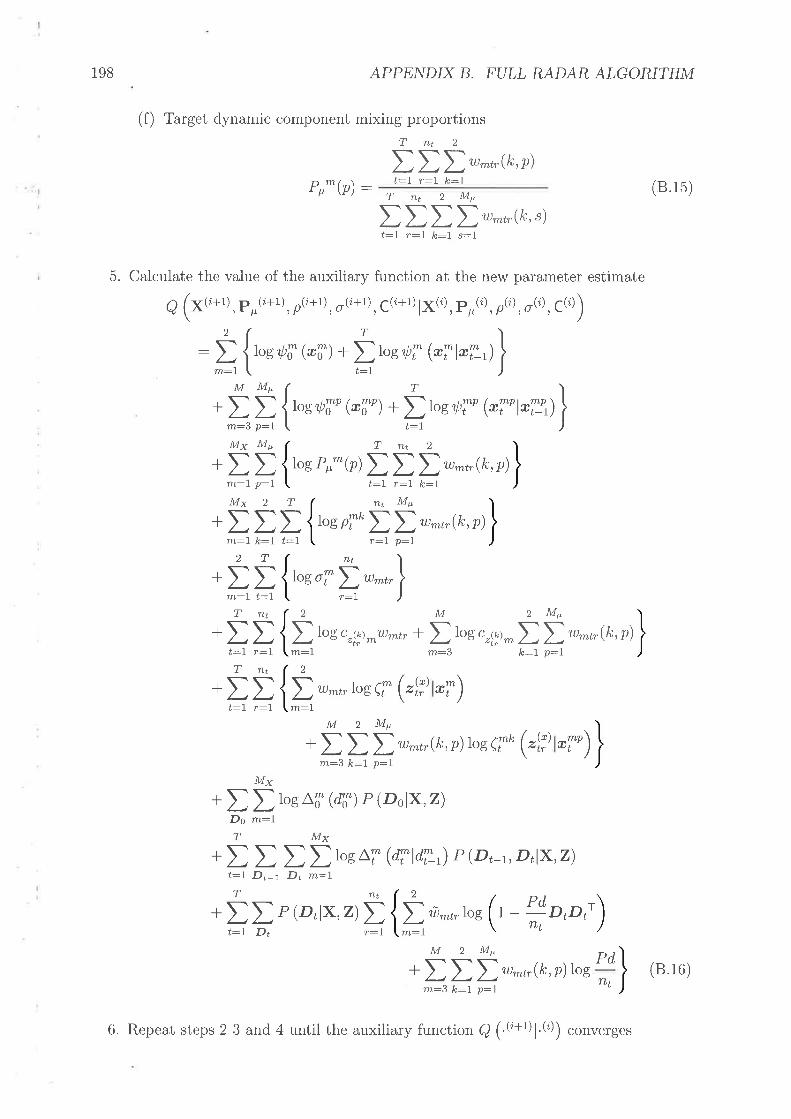
198 APPENDIX B. FULL RADAR ALGORITHM
(f) Target dynamic component mixing proportions
Pr^(P):
Tnt2
IIL'^*(k,p)t:I r:I k:I
Tru2Mt'
ttttw^¿,(k,s)t:I r:7 k:l s:l
5. Calculate the value of the auxiliary function at the new paraneter estimate
a (x{z+rl, p/.,(i+1) i p(i+I) , 6Q+t), ç(i+r; lx(i), pr(l) , ,(t') , oQ') , C@)
.,( T ì: t ltos,þi @i) + Dto* ,þî @il*T) I_-:, I t:r )MMp( r I
+ t f j t"*,þi' @To)+ t Ioe,þT' @T'l*Y) Im=3 p:r ( ¿:l )
M
m:3
2Mp
k:1 p:L
(8.15)
+tt IosPr-(p)ttT.-*(k,p)My2T
lulx Mp
m:7 p:l
m:l t:7Tnt
t:l r:LTnt
Tnt2
r:I p:I
t:I r:l k:Int Mp+ttt IoepT* tt w*t,(k,p)
rn:I k:7 t:l2T+tt togoiä.,-"j
2*It I to* c"Ík)^w-t + D ror""Í|,^t t w^¡(k,p)tn:l
+tt 2tm:l
Umtr ros (I (,Í? *f)M2Mp
+ t t D w^t (k,p)tos ef- ("Í? *f')t:7 r:1
v¡¿:l þ:! p:!My
+ I I to* Li @,T) P (Dolx,z)
My+ t t t D to*
^T @TldT,) P (o,-,, Dtlx,z)
Ds m:lT
t:I Dt-t D¡ m:IT
t:t Dt1- P-! prprt
rù¡+I\r (D,lX, z)Ð I ú-r" log
nt 2
r:1 m:1.M2Mp
+ttt umtr(k,p)los PdTL¡yy¡:f, þ:l p:t
6. Repeat steps 2 3 and 4 until the auxiliary function I (.(z+r¡1.(a)) converges
(8.16)
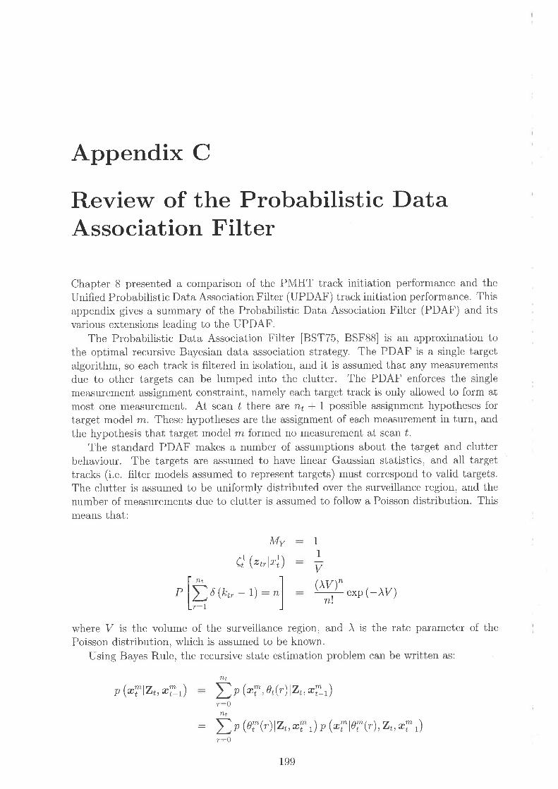
Appendix C
Review of the Probabilistic l)ataAssociation Filter
Chapter 8 presented a comparison of the PMHT track initiation performance and theUnified Probabilistic Data Association Filter (UPDAF) track initiation performance. Thisappendix gives a summary of the Probabilistic Data Association Filter (PDAF) and itsvarious extensions leading to the UPDAF.
The Probabilistic Data Association Filter [BST75, BSF88] is an approximation tothe optimal recursive Bayesian data association strategy. The PDAF is a single targetalgorithm, so each track is filtered in isolation, and it is assumed that any measutementsdue to other targets can be lumped into the clutter. The PDAF enforces the singlemeasurement assignment constraint, namely each target track is only allowed to form atmost one measurement. At scan ú there àtÊ 'n¿ * 1 possible assignment hypotheses fortarget model rn. These hypotheses are the assignment of each measurement in turn, andthe hypothesis that target model m formed no measurement at scan ú.
The standard PDAF makes a number of assumptions about the target and clutterbehaviour. The targets are assurned to have linear Gaussian statistics, and all targettracks (i.e. filter models assumed to represent targets) must correspond to valid targets.The clutter is assumed to be uniformly distributed over the surveillance region, and thenumber of measurements due to clutter is assumed to follow a Poisson distribution. Thismeans that:
My 1
1
P Ðd (*,, - r) :,nt
e| ("r,l"l) V
#exp(-Àrz)r:l
where I/ is the volume of the surveillance region, and À is the rate parameter of thePoisson distribution, which ìs assumed to be known.
Using Bayes Rule, the recursive state estimation problem can be written as:
nt
l,n (*7,0¡(r)lZ¿,æ7r)r:0nt
D,e (ef ?)12,,*7,) r (æiloiQ),2,,*7,)r:O
n (æilZ', n!t)
199

200 APPENDIX C. REVIEW OF PDAF
nt: Pf @ ,þT @Tl*7,) * D þiØ n (æilz,,,*7r), (c.1)r:l
where 0T(r) represents the rth assignment hypothesis at scan f and þT(r) is the posterior
probability of that hypothesis, and I 0iØ: 1. Under hypothesis 7iQ), measurement
r is caused by target model m and,ä:tÏotn., measurements are due to clutter - since thealgorithm is a single target one, any measurement not caused by model rn must be due toclutter, i.e. model 1. Under hypothesis 0T@) all measurements are due to clutter. Theterm p (*Tlrr,,æl1.r) in (C.1) is the probability density function of the target state whenit is updated by measurement z¡,. If the probability density of the state at the previousscan is Gaussian, then this expression can be gained through a Kalman Filter.
The density in (C.1) is clearly multimodal. If the prior state distribution is unimodal,then (C.1) will have k I I modes. This is the exponential growth in complexity ofthe Bayesian association approach. The PDAF makes the assumption that the density(C.1) can be approximated by a single Gaussian, thus reducing the distribution back to aunimodal one. The PDAF thus requires the mean and the variance of the posterior statedensity. First, consider the mean. Using (C.1), write:
E {æilz¡,æ1r} : øf Q) E {rTl*7r} + t 0iØ E {nilz¡,,*1r} . (c.2)nt
r:I
Using a Kalman Filter,
E {æ!lz¡,,æ7r} : E {nilæ\r} +wTi#,
where the innovalion, uff is given by
,# : l"r, - HT E {*Tl*I:'}) ,
and Wfl is the Kalman gain, which is independent of the measurement.Substituting (C 3) into (C.2) gives
rLt
E {æilZ¿,æ7r} prg) E {æilæi,} + I 0iØ ø {æilri,} +w7"ç
(c.3)
(c.4)
(c 5)
(c 6)
r:1nt
E {nilæi,} + I tsiØ wT,#r:1: E {rilæir} +w7"7,
where uf is a synthetic innovation given by
nt,i : \ 0f frl 1",, - ni n {æil*!r}lr:l
Comparing (C.5) with (C.3) it is clear that the mean of the track state posterior prob-ability density can be obtained using a single Kalman filter with a synthetic innovation.This provides for an efficient implementation for the mean update.

20t
Using similar manipulations, the covariance of the posterior state estimate can beshown [BSF88] to be
nt
cov {rilz,, æTr} : p#Pf Qlt - 1) + \, Of ef Oft)r:I
+wr \,ProvnzT' - 2Tzr' wTnt
r:lT (c 7)
where PT(tlt - 1) is the covariance of the state estimate given the previous state estimate,and Pi(tlt) is the covariance of the state estimate when it is updated by a measurementat scan ú and assignment is known (under this condition, the value of the measurementdoes not effect this covariance). Both of the covariances PT(tlt - 1) and Pfl(úlú) areprovided by the Kalman Filter, So, (C.7) can be viewed as a correction to the KalmanFilter Covariance to account for the data association uncertainty.
The PDAF is thus implemented using a Kalman Filter, with a synthetic innovation,and a correction to the posterior covariance. This means the PDAF is a very efficientalgorithm, carrying little extra cost than th.e optimal estimator when the assignments areknown.
Many of the Bff wlll be close to zero, and (C.11) is expensive to calculate becauseof the exponential. To reduce the computation load, it is usual practice to introducea validation gate, which is generally a physical boundary set at some multiple of theinnovation covariance, i.e.
(z-nieff-,)'sr-'Q-aieffi-t):12. (c.8)
Measurements outside this boundary are assumed to have negligible probability ofbeing due to the target. The number of measurements in the validation region thenreplaces n¿ in the above equations.
Let Pdi be the probability that target m is detected at scan ú. This probability maybe a function of the target state, especially in the case where physical obstacles mayobscure the target. Lef Pgi be the probability that a target measurement is within thevalidation gate, given that it was detected. Usually, the gate is chosen lo make Pglconstant.
There are two forms of the PDAF, known as the parametric and nonparametric PDAF.In the parametric PDAF, it is assumed that the rate parameter of the clutter density, À, isknown. In the nonparametric PDAF, the rate parameter is unknown and is approximatedusing \: mtlV. An alternative nonparametric PDAF in [CDAS6] uses the approximation),: ntlA where A is the area of the entire surveillance region. This latter form will bemore accurate, if the data really is uniformly distributed.
For the parametric PDAF, the association probabilities, 0T(r), are given by
piv): #-(')--, (c e)
Ðure)r:0
where
bT(0) Àlztrsilvz (r - Pdi Psi) (c.10)Pgi'
1, T:lr...rfutb?(,) exp
2>mIem-l:tnatr Jt zlr (c 11)

202 APPENDIX C. REVTEW OF PDAF
It is important to recognise that the association probabilities, Bi(r), use the innovationcovariance matrix, Sfl, not the measurement process ef O Thus, measurements areassigned based on the current state estimate uncertainty. This is both a boon and a banefor the PDAF. If a target manoeuvres, the state moves arvay from the predicted state andthe innovation covariance grows, allowing the PDAF to recapture the track. However,tracks started on clutter rnay be allowed to assign distant measurements because theinnovation covariance is large.
C.l Nearest Neighbour GatingIn the standard PDAF, a validation gate is used to restrict the number of possible assign-ment hypotheses, and hence the computational load. It is assumed that measurementsoutside the validation gate have a negligible probability of being caused by the target cor-responding to the track. The validation gate itself is usually deflned by the hyper-ellipse
(z - Hiri)'sf-' Q - Hini) : r'where Sf is the innovation covariance for track rn at scan ú and 12 is some fixed thresholdsetting. [Dru01] calls gating first stage data association.
The purpose of gating is primarily to remove the need to make costly density calcu-lations, such as eT Qr,l*T), for very distant measurements that obviously do not belongto the track. This need not be done by using a fixed radius hyper-ellipse. In [CDA86],Nearest Neighbour Gating was introduced. Here, each track validates the l measurementsclosest to it. The number of validated measurements is fixed, at 1, and the physical size ofthe effective validation region changes with each scan. This method was originally intro-duced to improve pipelining of the data association algorithm by removing the dynamicvariation in the number of assignment hypotheses. However, it has since shown to giveother advantages over a fixed gate [CD00a].
The main advantage of using a fixed number of validated measurements, rather thana spatially fixed gate, is that it makes the algorithm adaptive to the clutter conditions.When the clutter is low (i.e. there are very few false detections) then the effective gate isvery large, and it is possible to valiclate measurements distant from the extrapolated targetposition, such as may occur after a manoeuvre. When the clutter is high (i.e. there aremany false detections) then the effective gate is small, and the track is not easily seduced.While it is possible to design the gate based on the prevailing clutter condition, in practiceclutter varies with time and perhaps spatially. lCDOOa] demonstrated that using a lownumber of nearest neighbours, say 1 : 3, does not degrade tracking performance.
C.2 Target VisibilityThe standard PDAF makes the assumption that every track corresponds to a valid target.In practice this is an unrealistic assumption. Targets move out of the surveillance region ofthe sensor, and aircraft land. Thus, what begins as a track corresponding to a valid targetmay become a track corresponding to no target. Similarly, the target tracks must comefrom somewhere. Even if the tracks are initiated by a radar operator, it is inevitable thatthere will be some tracks that have been falsely initiated. A tracking filter for a realisticscenario should be able to deal with these conditions.
The target visibility model is a method for enabling the tracker to make automaticinitiation and termination decisions. The model was first introduced in [CDA86] and
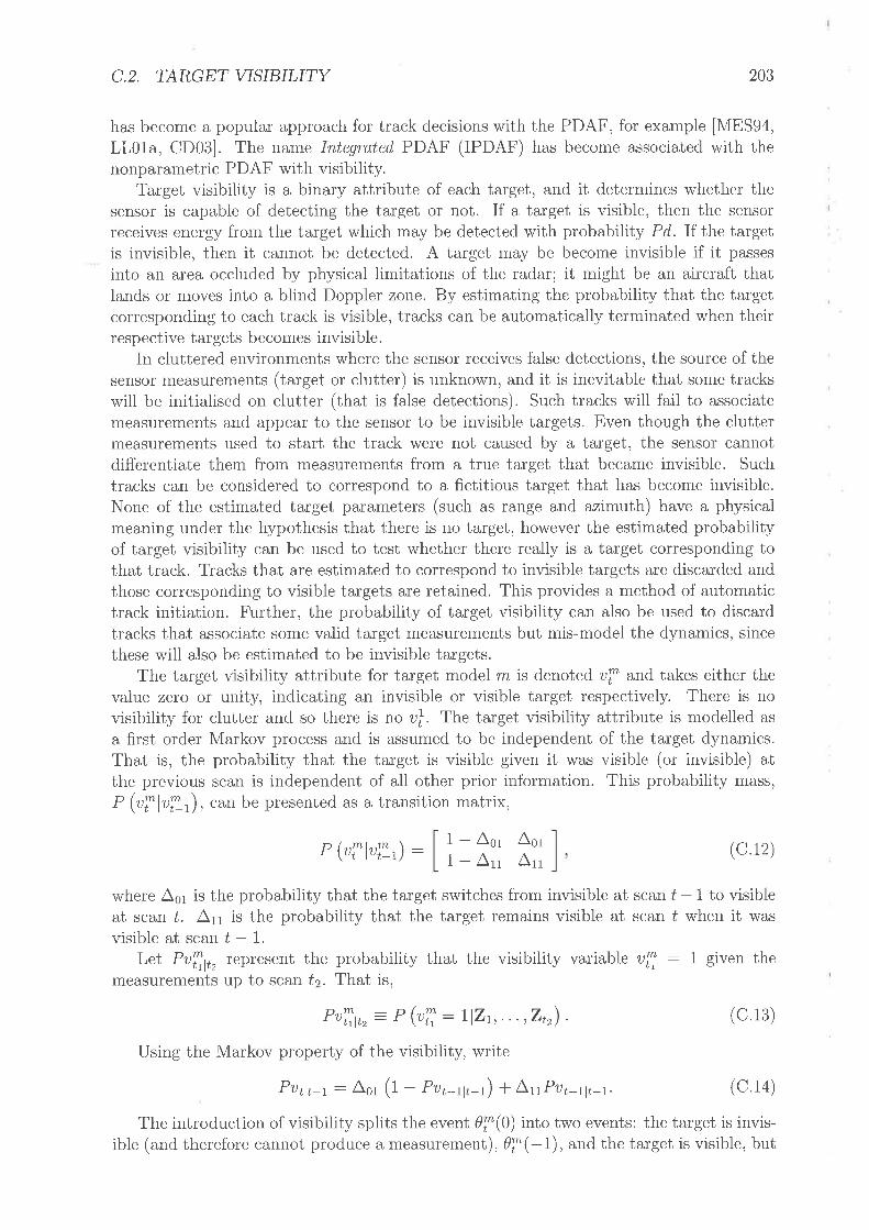
C.2. TARGET VISIBILITY
has become a popular approach for track decisions with the PDAF, for example [1\'IES94,LL01a, CD03]. The name Integrated PDAF (IPDAF) has become associated with thenonpararnetric PDAF with visibility.
Target visibility is a binary attribute of each target, and it determines whether thesensor is capable of detecting the target or not. If a target is visible, then the sensorreceives energy frorn the target which may be detected with probability Pd. H the targetis invisible, then it cannot be detected. A target may be become invisible if it passesinto an area occluded by physical limitations of the radar; it might be an aircraft thatlands or nÌoves into a blind Doppler zone. By estimating the probability that the targetcorresponding to each track is visible, tracks can be automatically terminated when theirrespective targets becomes invisible.
In cluttered environments where the sensor receives false detections, the source of thesensor measurements (target or clutter) is unknown, and it is inevitable that some trackswill be initialised on clutter (that is false detections). Such tracks will fail to associatemeasurements and appear to the sensor to be invisible targets. Even though the cluttermeasurements used to start the track were not caused by a target, the sensor cannotdifferentiate them from measurements from a true target that became invisible. Suchtracks can be considered to correspond to a fictitious target that has become invisible.None of the estimated target parameters (such as range and azimuth) have a physicalmeaning under the hypothesis that there is no target, however the estimated probabilityof target visibility can be used to test whether there really is a target corresponding tothat track. Tracks that are estimated to correspond to invisible targets are discarded andthose corresponding to visible targets are retained. This provides a method of automatictrack initiation. Further, the probability of target visibility can also be used to discardtracks that associate some valid target measurements but mis-model the dynamics, sincethese will also be estimated to be invisible targets.
The target visibility attribute for target model rn is denoted ui and takes either thevalue zero or unity, indicating an invisible or visible target respectively. There is novisibility for clutter and so there is no ur1. The target visibility attribute is modelled as
a first order Markov process and is assumed to be independent of the target dynamics.That is, the probability that the target is visible given it was visible (or invisible) atthe previous scan is independent of all other prior information. This probability mass)P (uiluir),
"utt be presented as a transition matrix,
203
P (uilui,) : 1 - Aor Aot1 - Arr Arr (c.12)
where 461 is the probability that the target switches from invisible at scan ú - 1 to visibleat scan ú. All is the probability that the target remains visible at scan ú when it wasvisible at scan t - L
Lef Puft¡t, represent the probability that the visibility variable ul : 1 given themeasurements up to scan ú2. That is,
Pullp" = P (uff : IlZt,. .. ,Zr,) (C.13)
Using the Markov property of the visibility, write
Prrlr-l.: Aor (t - Pur-tlr-r) + LryPu¡-1¡¡-1' (C.14)
The introduction of visibility splits the event 0?(0) into two events: the target is invis-ible (and therefore cannot produce a measurement),0iÇ1), and the target is visible, but

204 APPENDIX C. REVIEW OF PDAF
either undetected, or the detected measurement is not validated, 0iQ). The probabilityof the invisibility event is given by
bTer): Àt2trsrtp L!-u). (c.15)\ l'tt rt I pgT pu4t_t
and the other b's are unchanged (the normalisation equation for p now spans mi2 events).The updated visibility probability, Puff¿, is obtained using
Puff,: t - Pf er) (C.16)
The visibility model has been shown to provide a substantial reduction in false tracks[cDA86]
C.3 Augmented PDAFThe PDAF algorithm is derived for measurements that are a linear function of the targetstate, such as position and bearing estimates. In practical applications, there may be otherfeatures of the observed data that can be used to discriminate target measurements fromfalse detections due to clutter. The extension of the PDAF to deal with such informationis referred to as the Augmented PDAF [BSL95].
Suppose that the sensor provides features with each measurement, in addition to theusual state observation components. These features may be continuous valued or discrete,or a combination of both. The combined measurement vector can be written as
(c.17)
where .ti) i" a vector of state observations, and ,!!) i" a vector of features.Assume that the probability density (mass) function of the feature vector, ,[l) , i"
known for both targets and clutter. Denote these probabilities as c!likelihood ratio of the feature vector is
(,tf') Then, the
"r (,:P)
- -l "lî) \'tr-\'ä'I
L* (c 18)-(k)'tr
The augmented measurelnents are then incorporated by multiplying (C.11) by theIikelihood ratio, L* (r[?)
bT?) : L (4f') ",{-;uT'sT-'zT}, r : t,...,,,t. (c.le)
C.4 Sophisticated Clutter ModelsThe standard PDAF makes the assumption that the clutter is uniformly distributed. Thisassumption is rarely accurate. For most sensors, the distribution of false detections is afunction of at least one of the measurement components. For example, false detections aremore likely at low elevation angles for a ground based radar, or at low Doppler frequencies.
(kutr( ) cl
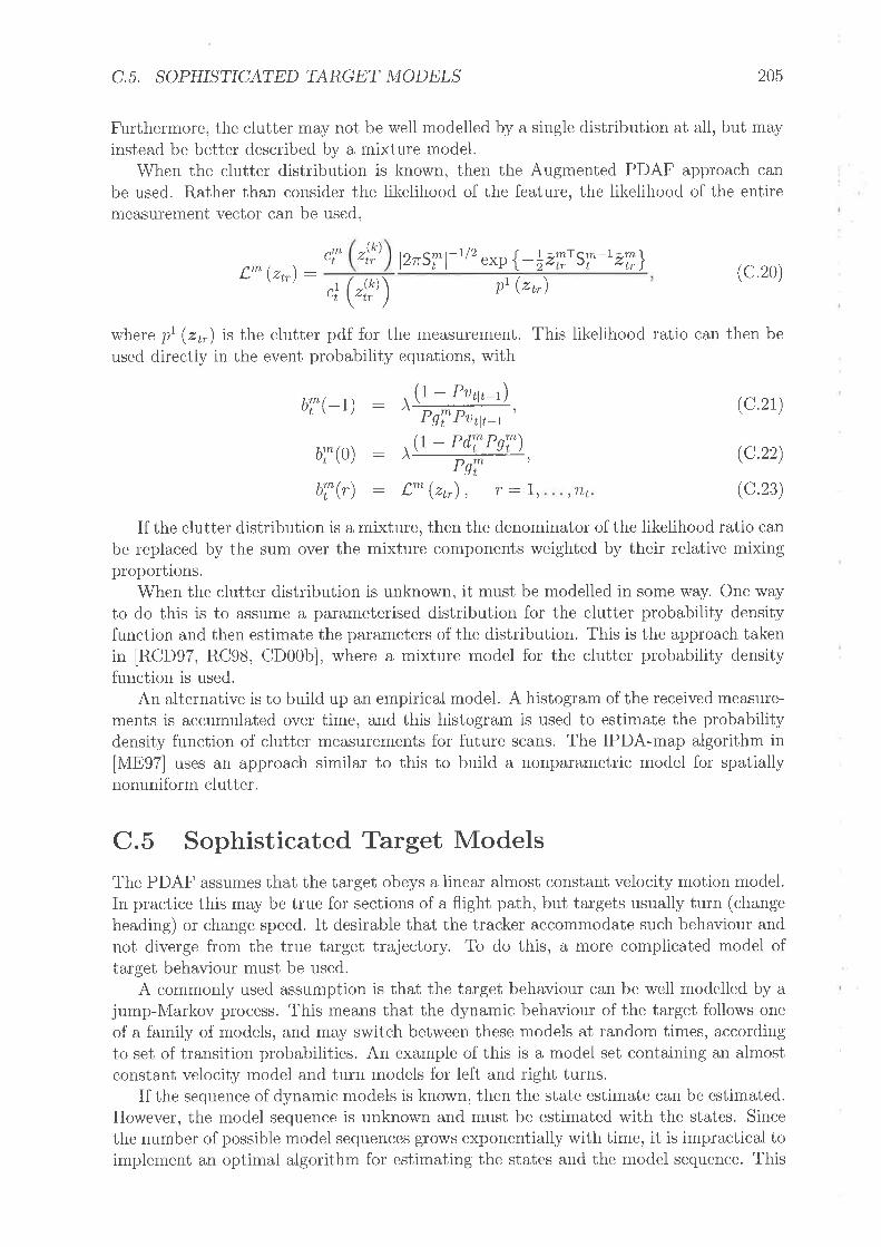
C.5, SOPHISTICATED TARGET MODELS 205
Furthermore, the clutter may not be well modelled by a single distribution at all, but mayinstead be better described by a mixture model.
When the clutter distribution is known, then the Augmented PDAF approach canbe used. Rather than consider the likelihood of the feature, the likelihood of the entiremeasurement vector can be used,
L- (z¡r) :ci l/çlzìr' l2rST al t 2 exp {- t zff. ST -' zi.} (c 20)
"r (":P) pr (z*)
where pr (zr,) is the clutter pdf for the measurement. This likelihood ratio can then beused directly in the event probability equations, with
(t - Pr,,,, .\bTeL) : xffi, (c2r)
. (1 - rdiPsi)b;í"(0) : ^t--#:tbT(r) : L^("t), r:L, ,frt
(c.22)
(c.23)
If the clutter distribution is a mixture, then the denominator of the likelihood ratio canbe replaced by the sum over the mixture components weighted by their relative mixingproportions.
When the clutter distribution is unknown, it must be modelled in some way. One wayto do this is to assume a parameterised distribution for the clutter probability densityfunction and then estimate the parameters of the distribution. This is the approach takenin [RCD97, RC98, CD00b], where a mixture model for the clutter probability densityfunction is used.
An alternative is to build up an ernpirical modei. A histogram of the received measure-ments is accumulated over time, and this histogram is used to estimate the probabilitydensity function of clutter measurements for future scans. The IPDA-map algorithm in[Ìv'IE97] uses an approach similar to this to build a nonparametric model for spatiallynolruniform clutter.
C.5 Sophisticated Target ModelsThe PDAF assumes that the target obeys a linear almost constant velocity motion model.In practice this may be true for sections of a flight path, but targets usually turn (changeheading) or change speed. It desirable that the tracker accommodate such behaviour andnot diverge frorn the true target trajectory. To do this, a more complicated model oftarget behaviour must be used.
A commonly used assumption is that the target behaviour can be well modelled by ajump-Markov process. This means that the dynamic behaviour of the target follows oneof a family of modcls, and may switch between these models at random times, accordingto set of transition probabilities. An example of this is a model set containing an almostconstant velocity model and turn models for left and right turns.
If the sequence of dynamic models is known, then the state estimate can be estimated.However, the model sequence is unknown and must be estirnated with the states. Sincethe number of possible model sequences grows exponentially with time, it is impractical toimplement an optimal algorithm for estimating the states and the model sequence. This
206 APPENDIX C. REVIEW OF PDAF
(c.25)
is very similar to the problem encountered with the visibility Markov model for trackdecisions as described in chapter 2. However, whereas the visibility model is a switchingmodel controlling the target observatiorì process, this is a switching model controlling thestate evolution process.
Like the visibility model, the problem of switching target dynamics can be solvedusing an IMM-PDAF [\,'IABSD98]. As described in chapter 2, the IMM-PDAF is anapproximation to a generalised pseudo Bayes order 2 approach.
An alternative to the IMNI is presented in [Col99]. This fllter uses a first order GPBstructure. The first order GPB approach is simpler than the IMM structure, but IMM isgenerally considered to give superior performance for manoeuvring targets [BSL95].
C.6 The Unified PDAFThe Multiple Model Unified PDAF (MM-UPDAF) lCD03] is a nonparametric PDAF thatincorporates nearest neighbour validation, multiple nonuniform clutter models, multipletarget dynamic models and target visibility. This algorithm is used in the operationalJFAS detection and tracking software. The event probabilities for the MM-UPDAF aredenoted bV /io (r), where m is a track index, p is a model index, and r is the measurementindex. Since the algorithm is a single target one, Bie(r) is assumed to be independent ofB¡nl(s)tfnlm.
The JFAS system uses a preprocessor that tags each measurement as being caused byclutter component L or 2. This tagging procedure is assumed to be perfect. The eventprobabilities for target models m > 2 are given by
1io (r)uT'(r) (c.24)MpI
ttbr'(i')s:l i:l
where
bT',eI)
bTo(0)
,*7"#,P^T' 0 - Pdfe PtTo) , (c.26)
bìir,,e(r) : pmip pd,irÇi1?"1"T)-"i'qî ." : "(,!\. ç.27)' *L Cf e"lr",) Nf I t u - zLr .
Models 1 and 2 are used to represent clutter. The term P^T'is the a priori probabilityfor model p, PsTo is the probability that the target orientated measurement is within the1 nearest, given model p is the correct model, nf is the number of measurements taggedas type c from those within the 1 nearest for all models, Nr" is the total number ofmeasurements tagged as type c and ,4f is the spatial area of the component c (providedby the preprocessor).
The derivation of these expressions is presented in detail in [Col99].
C.7 The Joint UPDAFThe MM-UPDAF makes a single target approximation, namely that the assignment ofmeasurements can be performed independently for different target tracks. This assump-tion is invalid when targets are closely spaced with respect to the sensor resolution. This

C,7. THE JOINT UPDAF 207
circumstance may also arise in OTHR when multiple propagation paths are closely spaced,In order to improve the tracking performance of the MM-UPDAF, this single target as-
sumption was relaxed and a Multiple Model Unified Joint PDAF was developed [DC01].The event probabilities for this filter are found using substantially more complicated ex-pressions than those above, and are not presented here.

208 APPENDIX C. REVIEW OF PDAF

Bibliography
H Akaike, A new look at the stat'ist'ical model'identi,ficati,on, IEEE transca-tions on Automatic Control 19 (1974), no. 6, 7L6 723.
B D O Anderson and J B Moore, Opti,mal filtering, Prentice Hall, 1979.
H A P Blom and Y Bar-Shalom, The 'interacti,ng mult'iple model algori,thm
for sgstems u,th markoutan swi,tch'ing coefficr,ents, IEEE transcations on Au-tomatic Control 33 (1988), no. 8, 780-783.
[Ben81] V E Benes, Eract fin'ite-di,mens'ional f,lters wi,th certai,n di,ffusi.on non I'ineardrift, Stochastics 5 (1931) , 65-92.
[Ber7e] D P Bertesakas, A dtstri,buted algori,thm for the ass'ignment problem, Labfor information and decision systems working paper, MIT, March 1979.
IBer8s] D P Bertsekas, The aucti,on algorithm: A d'istributed relarat'ion method forthe assi,gnment problem, Ãnnals of Operations Research: special issue onparallel optimisation 14 (1938), 105-123.
[Aka7a]
IAM7e]
lBBSs8l
[BIa86]
[BIo8a]
IBPee]
lBSCBeol
[BSCLeo]
lBSF8sl
S S Blackman,, Multr,ple target tracking wi,th radar appli,cat'ions, Artec House,Norwood, Massachusetss, USA, 1986.
H A P Blom, An ffic'ient fi,lter for abruptlg chang'ing systems,23rd confer-ence on decision and control (Las Vegas, Nevada, USA), December 1984.
S S Blackman and R Popoli, Desi,gn and analysi,s of modern tracki,ng systems,Artec House, Norwood, Massachusetss, USA, 1999.
Y Bar-Shalom, K C Chang, and H A P BIom, Multi,target-multi,sensor track-i,ng: Appl'icat'ions and aduances, vol. L, ch. 2: Automatic track formationin clutter with a recursive algorithm, pp. 25 42, Artech House, Norwood,Massachusetss, USA, 1990.
Y Bar-Shalom, L J Campo, and P B Luh, From rece'iuer operati,ng charac-tertst'ic to sgstem operat'ing characterist'ic: Eualuati,on of a track formati,onsystem,IEEE transcations on Automatic Control 35 (1990), no. 2,I72-I79.
Y Bar-Shalom and T E Fortman, Track'ing and data assoc'iat'ion, AcademicPress, San Diego, California, USA, 1988.
Y Bar-Shalom and X R Li, Effecti,ueness of the li,keli,hood functi,on i,n logi,c-based track format'ion, IEEE transactions on Aerospace and Electronic Sys-tems 27 (1991), no. 1, I84-I87.
[BSLe1]
209

210
[BSLe5]
[BSr75]
Iccee]
[cco1]
[CD00a]
[cDoob]
lcDo3l
lcDAs6l
lcDDe6l
ICEWeaa]
lcEwe4bl
[CEweac]
ICha00]
lcKBSoll
ICol87]
BIBLIOGRAPHY
, Multi,target-mult'isensor track'ing: pri,nci,ples and techn'iques, YBS,Storrs, Conneticut, USA, 1995.
Y Bar-Shalom and E Tse, Track'ing in a cluttered enutronment wtth proba-bi,li,sti,c data assocr,atton, Automatica 11 (1975).
C K Chui and G Chen, Kalman fi,lteri,ng w'ith real-ti,me appl'icat'ions, Springer-Verlag, Berlin, Germany, 1999.
S B Colegrove and B Cheung, A peak detector that p'icks more than peaks,Radar, 2001.
S B Colegrove and S J Davey, On us'ing nearest ne'ighbours w'ith the proba-bi,li,sti,c data associ,ati,on filter, Radar, 2000, pp. 53 58.
, The probab'ili,st'ic data assoc'iat'ion fi,lter w'ith mult'iple nonuni,formclutter reg'ions, Radar, 2000, pp. 65 70.
, PDAF wi.th multi,ple clutter regi,ons and target models,IEEE trans-actions on Aerospace and Electronic Systems 39 (2003), no. 1, LL0-I24.
S B Colegrove, A W Davis, and J K Ayliffe, Traclc initi,ati,on and nearestne'ighbours 'incorporated'into probab'il'isti,c data associ,ati,on, Journal of EIec-trical Electronics Engineering, Australia 6 (1986), no. 3, 191-198.
S B Colegrove, L M Davis, and S J Davey, Performance assessrnent of track-ing systems, International Symposium on Signal Processing and its Appli-cations (Gold Coast, Australia), vol. 1, August 1996, pp. 188-192.
B D Carlson, E D Evans, and S L Wilson, Search radar detect'ion and trackw'ith the hough transform I: System concept,IEEE transactions on Aerospaceand Electronic Systems 30 (1994), no. 1, 102 108.
, Search radar detect'ion and track w'ith the hough transform II: De-tect'ion stat'ist'ics, IEEE transactions on Aerospace and Electronic Systems30 (1994), no. 1, 109-115.
, Search radar detecti,on and track w'ith the hough transform III: De-tecti,on performance uith b'inary i,ntegrat'ion IEEE transactions on Aerospaceand Electronic Systerns 30 (1994), no. 1, lL6-t25.
S Challa, Target tracki,ng i,ncorporati,ng fl,i,ght enuelope i,nformatr,on, Pro-ceedings of the 3rd International Conference on Information Fusion (Paris,France),2000.
H Chen, T Kirubarajan, and Y Bar-Shalom, Mult'iple low obseruable balli,s-ti,c m'issi,le track i,n'it'iat'ion us'ing an ESA radar, ESP lab technical report,University of Conneticut, March 2001.
S B Colegrove, Mult'itarget track'ing i,n a cluttered enu'ironment,InternationalSymposium on Signal Processing and its Applications (Brisbane, Autralia),1987.

BIBLIOGRAPHY
ICol8e]
IColes]
ICol00]
[cPo1]
[cvwo2]
ldcosl
[DCee]
217
, Austrah,an deuelopments on tracki,ng 'in a cluttered enutronmentIEEE International Conference on Control and Applications, April 1989.
, Aduanced Ji,ndalee tracker: probabi,l'isti,c data assoc'iat'ion multi.plemodel'intt'iatton filter, Technical report TR-0659, Defence Science and Tech-nology Organisation, Australia, June 1999.
, Project jindalee: from bare bones to operat'ional OTHR, Radar, 2000,pp.825 830.
S Challa and G W Pulford, Jo'int target track'ing and classr,ficati,on usi,ngradar and ESM sensors,) IEEE transactions on Aerospace and ElectronicSystems 37 (2001), no. 3, 1039-1055.
S Challa, B Vo, and X Wang, Bayes'ian approaches to track eristence - IPDAand random sets, Proceedings of the Sth International Conference on Infor-mation Fusion (Annapolis, Maryland, USA) , July 2002.
M de Cervantes, Don Qui,rote de la Mancha, L605.
S J Davey and S B Colegrove, Aduanced J'indalee tracker: Enhanced pealc
detector, Technical report TR-0765, Defence Science and Technology Organ-isation, Australia, June 1999.
, A unr,fi,ed jo'int probabi,l'ist'ic data assoc'iat'ion fi,lter w'ith multi,ple mod-els, Technical report TR-l184, Defence Science and Technology Organisa-tion, Australia, June 2001.
A Doucet, N De Freitas, and N Gordon, Sequenti,al monte carlo methods i,npract'ice, Springer Verlag, April 2001.
R O Duda and P E Hart, Use of the hough transformat'ion to detect ltnes andcurues i,n pi,ctures, Communications of the ACM 16 (1972), no. 1, 11-15.
D T Dunhanr and R G Hutchins, Track'ing mult'iple targets i,n cluttered enui-ronments wzth a probab'il'ist'ic mult'i-hypothes'is tracker, Tracking and PointingXI (SPIE Annual International Symposium on Aerosense, Orlando, Florida,USA), vol. SPIE 3086, April 1997, pp. 284-295.
A P Dempster, N M Laird, and D B Rubin, Marimum li,keli,hood from in-complete data ui,a the EM algorithm, Journal of the Royal Statistics Societyr4o (7977), 1-38.
O E Drurnmond, On features and attributes i,n mult'isensor, mult'itarget traclc-tng, Proceedings of the 2nd International Conference on Information Fusion(Sunnyvale, California, USA), 1999, pp. 1045-1053.
, Feature, attribute, and class'ificat'ion ai,ded target track'ing, Signaland Data Processing of Small Targets (San Diego, California, USA), vol.SPIE 4473, July 2001, pp. 542-558.
A Farina, D Benvenuti, and B Ristic, A comparati,ue study of the Benes
fi,lteri,ng problem, Signal Processing 82 (2002), 133 I47 .
lDColl
IDDFGol]
lDH72l
[DHe7]
lDLRTTI
[Drue9]
[DruO1]
IFBRo2]

IHDe7]
212 BIBLIOGRAPHY
[FBSSS3] T E Fortman, Y Bar-Shalom, and M Scheffe, Sonar tracki,ng of mult'ipletargets usi,ng jo'int probabi,li,sti,c data associati,on, IEEE Journal of OceanicEngineering 8 (1983) ,173-784.
[FFee] L Frenkel and M Feder, Recurs'iue Erpectatr,on-Marim'istai,on (EM) algo-rithms for t'ime-uary'ing parameters w'ith appli,cat'ions to mult'iple target track-'ing, IEEÐ transactions on Aerospace and Electronic Systems 47 (1999),no. 2,306-320.
M L Fisher, The Lagrangr,an relarati,on method for soluing i,nteger prograrn-m'ing problems,Management Science 27 (1981), no. 1, 1-18.
G D Forney Jr, The u'iterbi, algorithm, Proceedings of the IEEE 61 (1973),no. 3, 268-278.
[Fis81]
IFr73]
lGMFo2l A Gad, F Majdi, and M Farooq, A comparison of data assoc'iat'ion techn'iquesfor target track'ing 'in clutter, Proceedings of the 5th International Conferenceon Information Fusion (Annapolis, Maryland, USA), July 2002, pp. 1126-1133.
[GRo1] N Gordon and B R Ristic, Tracki,ng a'irborne targets occasi,onally h'idden'inthe bli,nd doppler, Signal and Data Processing of Small Targets (San Diego,Calfiornia, USA), vol. SPIE 4473, JuIy 2001, pp. 587 595.
R G Hutchins and D T Dunham, Eualuat'ion of a probabi,listi,c mult'i-hypothes'is tracki,ng algortthm 'in cluttered enu'ironments, Thirtieth AsilomarConference on Signals, Systems and Computers (Los Alamitos, California,USA) , vol. 2,1997, pp. 7260-1264.
lHLBeTl Z Hu, H Leung, and M Blanchette,, Stat'ist'ical performance analys'is of track'in'iti,at'ion techn'iques, IEEE transcations on Signal Processing a6 (1997),no.2,445-456.
[HLPol] C Hue, J-P Le Cadre, and P Pérez, The (MR)MTPF: partzcle filters totrack mult'iple targets using multi,ple rece'iuers,Information Fusion (Montreal,Canada) , voL 2, August 2001.
[HLP02] , Sequent'ial mente carlo methods for multi,ple target tracki,ng and datafus'ion,,IEEE transcations on Signal Processing 50 (2002), no. 2,309-325.
[rK88] J Illingworth and J Kittler, A suruey of the hough transform, ComputerVision, Graphics, and Image Processing 44 (1983), 87 116.
S P Jacobs and J A O'Sullivan, H'igh resolut'ion radar models for jo'int track-'ing and recogn'it'ion, IEEE International Radar Conference (Syracuse, NewYork, USA), May 1997, pp. 99-104.
uoeTl
uR86l B Jang and L Rabiner, An 'introduct'ion to hi,dden markou models, IEEEASSP Magazine (1986).
R Jonker and A Volgenant, A shortest augment'ing path algori,thm for denseand sparse l'inear ass'ignment problems, Journal of Computing 38 (1937),325 340.
uvsTl

BIBLIOGRAPHY
IKal60]
lKB61l
IKGe7a]
IKGe7b]
[Krees]
[Kure0]
lLBSe0l
[LBSol]
[LHBe6]
[LKHe7]
ILLO1a]
lLLolbl
ll,swoll
ILees7]
273
R E Kalman, A neu approach to l'inear fi,lteri,ng and pred,i,ction problems,Journal of Basic Engineering 82 (1960),34-45.
R E Kalman and R Bucy, New results i,n li,near filtering and predi,cti,on prob-lems, Jotnnal of Basic Engineering 83 (1961), 95-108.
M L Kreig and D A Gray, Comparison of probabi,li,sti,c least squares andprobabzl'ist'ic mult'i-hgpothesi,s tracking algori,thms for mult'i-sensor traclc'ing,IEtrE International Conference on Acoustics, Speech and Signal Processing(Munich, Germany), vol. 1, April 1997, pp. 515 518.
, Multi,-sensor probabi,l'ist'ic multt-hEpothesi,s tracki,ng us'ing d'issi,mi,larsensorsr Proceedings of the Conference on Acquisition, Tracking and Point-ing XI, SPIE Symposium on Aerosense (Orlando, Florida, USA), vol. SPIE2086, April 1997, pp. 129 138.
M L Kreig, Probab'ili,sttc assoc'iat'ion and fus'ion for multi,-sensor trackingappli,cati,ons, Ph.D. thesis, Department of Electrical and Electronic Engi-neering, the University of Adelaide, Adelaide, South Australia, 1998.
T Kurien, Mult'itarget-multtsensor tracking: Appli,cat'ions and aduances,vol. 1, ch. 3: Issues in the Design of Practical Multitarget Tracking Al-gorithms, pp. 43 ?, Artech House, Norwood, Massachusetss, USA, 1990.
D Lerro and Y Bar-Shalom, Automat'ic track'ing uith target ampl'itude fea-ture, American Control Conference (San Diego, California, USA), 1990.
, Interact'ing multr,ple mod,el traclc'ing wi,th target ampl'itude feature,IEEE transactions on Aerospace and Electronic Systems 29 (2001) , no. 2,494 509.
M L Lees, An oueru'iew of s'ignal process'ing for an ouer-the-horizon radarinthe HF band,Inlernational Syrnposium on Signal Processing and its Appli-cations (Brisbane, Australia), 1987.
H Leung, Z Hu, and M Blanchette, Eualuat'ion of mult'iple target track i,ni,-tzati,on techn'iques i,n real rad,ar track'ing enu'ironments,IEE Proceedings onRadar, Sonar Navigation? 143 (1996) , no. 4,246-254.
A Logothesis, V Krishnamurthy, and J Holst, On maneuuring target tracktngu'ia the PMHT, Thirty-Six Conference on Decision and Control (San Diego,California, USA), December Igg7.
N Li and X R Li, Target percezuab'il'ity and 'its appli,cat'ion,IEEE transcationson Signal Processing 49 (2001), no. 11, 2588 2604.
, Tracleer desi,gn based, on target perce'iuabi,li,ty,IEEE transactions onAerospace and Electronic Systems 37 (2001), no. 1, 2I4 225.
T E Luginbuhl, Y Sun, and P Willett, A traclc rnanagernent system forthe PMHT algorithm, Proceedings of the 4th lnternational Conference onInforrnation Fusion (Montreal, Canada), August 2001.
T tr Luginbuhl, Personal Correspondence,2001.[LugOi]
274
[MABSDeS]
lMtre7l
[MESe4]
[MKe7]
IMor77]
[NSC84]
lPLeTl
[PPKoo]
[RAoo]
IRCe8]
IRCDe7]
IRei77]
[Rei7e]
IRis78]
BIBLIOGRAPHY
E Mazor, A Averbuch, Y Bar-Shalom, and J Dayan, Interact'ing mult'iplemodel methods 'in target trøcki,ng: & surueA) ItrEE transactions on Aerospaceand Electronic Systems 34 (1998), no. 1, I02 I23.
D MuËicki and R Evans, Data assoctatton us'ing clutter map 'informat'ion,Workshop on Signal Processing Applications (Brisbane, Australia), Decem-ber 1997, pp.227-230.
D Mu5icki, R Evans, and S Stankovic, Integrated probabi,li,st'ic data assoc'ia-ti,on,IEEE transcations on Automatic Control 39 (1994), no. 6, 1237-1241.
G J Mclachlan and T Krishnan, The em algori,thm and ertenszons, WileyInterscience, 1997.
C Nlorefield, Appl'icati,on of 0-f integer programm'ing to mult'i-target trackr,ngproblems,IEEE transcations on Automatic Control 22 (1977), no. 6, 302-3r2.
V Nagarajan, R N Sharma, and M R Chidambara, An algorithm for track-r,ng a manoueuering target 'in clutter,IEEE transactions on Aerospace andElectronic Systems 20 (1984), 560-573.
G W Pulford and A Logothesis, An erpectat'ion-mari,m'isat'ion tracker formult'iple obseruattons of a s'ingle target'in clutter, Thirty-sixth IEEE Confer-ence on Decision and Control (San Diego, California, USA), December lgg7,pp. 4997-5003.
K R Pattipati, R L Popp, and T Kirubarajan, Mult'itarget-mult'isensor track-i,ng: Appli,cat'ions and aduances, vol. 3, ch. 2: Survey of Assignment Tech-niques for Multitarget Tracking, pp. 77-159, Artech House, Norwood, Mas-sachusetss, USA, October 2000.
B Ristic and S Arulampalam, Mult'itarget m'irture reduct'ion algori'thm uithi,ncorporated target eristence recurs'ions, Signal and Data Processing of SmallTargets, vol. SPIE 4048,2000, pp. 357-368.
B Ristic and Colegrove, Modelli,ng the d'istribut'ion of false detecti'ons fortarget track'ing w'ith an OTHR,International Radar Symposium (Munich,Germany), vol. 3, sep 1998, pp. II47-1I54.
B Ristic, S B Colegrove, and S J Davey, Segmentat'ion of the suruei'llancearea of a skgwaue OTHR for track'ing 'in ampl'itude, \Morkshop on SignalProcessing Applications (Brisbane, Australia), 1997, pp.243 246.
D B Reid, A mult'iple hypothes'is f,lter for track'ing multi,ple targets i'n a clut-tered enu'ironment, Report LMSC,D-560254, Lockhead Missiles and SpaceCompany, September 1977.
., An algori,thm for tracki,ng multi,ple targets, IEEE transcations onAutomatic Control 24 (1979), 843-854.
J Rissanen, Model'ing by shortest data description, Automatica 14 (1978),465-47L.
BIBLIOGRAPHY
[Rw01a]
lRwolbl
[RwSesa]
215
Y Ruan and P Willett, An'improued PMHT usi,ng an'idea from codzng,200IAerospace Conference (Big Sky, Montana, USA), March 2001.
, Manoeuuri,ng PMHTs, Signal and Data Processing of Small Targets(SPIE Annual International Symposium on Optical Science and Technology,San Diego, California, USA), vol. SPIE 4473, July 2001, pp. 4L6 427.
C Rago, P Willett, and R L Streit, A comparison of the JPDAF and PMHTtrack'ing algori,thms, International Conference on Acoustics, Speech and Sig-nal Processing (Detroit, Michigan, USA), 1995, pp.357L 3574.
Y Ruan, P Willett, and R L Streit, A compari,son of the PMHT and PDAFtrackr,ng algorithms based on the'ir model CRLBs, SPIE Conference on Ac-quisition, Tracking and Pointing XIII (Orlando, Florida, USA), vol. SPIE3692, L999, pp. 177 188.
D J Salmond, M'irture reduct'ion algorithms for target tracki,ng 'in clutter,Signal and Data Processing of Small Targets, vol. SPIE 1305, 1990, pp. 434-445.
G Schwartz, Est'imati,ng the d'imensi,on of a model, Annals of Statistics 6(1978), no.2,46L 464.
R L Streit, M Graham, and M J Walsh, Multi,ple target tracki,ng of d'istributedtargets us'ing H'istogram-PMHT, Proceedings of the 4th International Con-ference on Information F\rsion (Montreal, Canada), August 2001.
B W Silverman, Dens'ity est'imat'ion for stati,st'ics and data analyszs, Chap-man and Hall/CRC, 1986.
R W Sittler, An opt'imal data assoc'iat'ion problem 'in surueillance theorg,IEEE transactions on Military Electronics MIL-8 (1964) ,125-139.
R L Streit and T E Luginbuhl, Probabr,listtc multt-hypothes'is trackr,ng, Tech-nical report 70428, NUWC, Newport, Rhode Island, USA, February 1995.
R L Streit, Track'ini,ti.ali,zati,on sens'it'iui,tg 'in clutter, Technical report L0426,NUWC, |Jewport, Rhode Island, USA, February 1995.
, Personal Correspondence, 2000
, Tracki,ng on i,ntensttg-modulated data streams, Technical report77227, NUWC, Newport, Rhode Island, USA, May 2000.
, Tracki,ng targets wi,th spec'ified spectra usi,ng the H-PMHT algorithm,Technical report lL29I, NUWC, Newport, Rhode Island, USA, June 2001.
[RWS95b] , Direct data fus'ion us'ing the PMHT, American Control Conference(Seattle, Washington, USA), 1995, pp. 1678 1682.
[Rwsee]
ISale0]
ISch78]
[sGwo1]
Isil86]
Isit64]
[sLe5]
IStrooa]
IStroob]
[Strol]
IStreb]
ITKee] S Theodoridis and Koutroumbas K, Pattern recogn'iti,on, Academic Press,1999.
2t6
lvit6Tl
[vLoo]
[vLKoo]
IWRSesa]
[wRSesb]
BIBLIOGRAPHY
A J Viterbi, Error bounds for conuoluti,onal codes and an asymptotr,callyopt'imum decod'ing algori.thm,IEEE transcations on Information Theory 13(1967), no.2,260-269.
N Vlassis and A Likas, An EM-VDM algori,thm for gauss'ian m'irtures uithunknown number of components, 'Iechnical report, Computer Science In-stitute, University of Amsterdam, Intelligent Autonomous Systems, TheNetherlands, April 2000.
N Vlassis, A Likas, and B Krose, Mult'iuari,ate gauss'ian m'irture modeli,ngwi,th unlcnown number of components, Technical report, Computer ScienceInstitute, University of Amsterdam, Intelligent Autonomous Systems, TheNetherlands, April 2000.
P Willett, Y Ruan, and R L Streit, The PMHT for manoeuuring targets,Signal and Data Processing of Small Targets (SPIE Annual InternationalSymposium on Aerosense, Orlando Florida, USA), vol. SPIE 3373, 1998,pp.416-427.
, A uariety of PMHZs, Workshop commun GdR ISIS (GT 1) andNUWC, approaches probabilistes pour l'extraction multipistes, November1998.
[YBSPD95] M Yeddanapudi, Y Bar-Shalom, K R Pattipati, and S Deb, Ball'ist'ic m'iss'iletrack'in'itiat'ion uith satell'ite obseruat'ions, IEEE transactions on Aerospaceand Electronic Systems 31 (1995), no. 3, 1054-1071.
lzBesl B Zhott and N K Bose, An effic'ient algori,thm for data assoc'iati,on i.n multi,-target track'ing,IEEE transactions on Aerospace and Electronic Systems 31(1995), no. 1,458 468.