The Burr XII Negative Binomial Distribution with Applications to Lifetime Data

International Journal of Statistics and Probability; Vol. 4, No. 1; 2015ISSN 1927-7032 E-ISSN 1927-7040

Published by Canadian Center of Science and Education

The Burr XII Negative Binomial Distribution withApplications to Lifetime Data

Manoel Wallace A. Ramos1, Ana Percontini1, Gauss M. Cordeiro2 & Ronaldo V. da Silva1

1Programa de Pos-Graduacao em Matematica Computacional, Universidade Federal de Pernambuco, Brazil2Departamento de Estatıstica, Universidade Federal de Pernambuco, Brazil

Correspondence: Manoel Wallace A. Ramos, Programa de Pos-Graduacao em Matematica Computacional, Uni-versidade Federal de Pernambuco, Cidade Universitaria, 50740-540 Recife, PE, Brazil.E-mail: [email protected]

Received: December 26, 2014 Accepted: January 12, 2015 Online Published: January 17, 2015

doi:10.5539/ijsp.v4n1p109 URL: http://dx.doi.org/10.5539/ijsp.v4n1p109

Abstract

A five-parameter model, called the Burr XII negative binomial distribution, is defined and studied. The new modelcontains as special cases some important lifetime distributions discussed in the literature, such as the log-logistic,Weibull, Pareto type II and Burr XII distributions, among several others. We derive the ordinary and incompletemoments, generating and quantile functions, mean deviations, reliability and two types of entropy. The orderstatistics and their moments are investigated. The method of maximum likelihood is proposed for estimating themodel parameters. We obtain the observed information matrix. An application to real data demonstrates that thenew distribution can provide a better fit than other classical lifetime models.

Keywords: Negative Binomial distribution, Burr XII distribution, Maximum likelihood, observed informationmatrix

1. Introduction

The negative binomial distribution has been widely used in mixing procedures of distributions. Several new modelshave been proposed and applied in survival analysis. Percontini et al. (2013) pionnered a family of univariatedistributions generated by compouding the negative binomial distribution with any continuos model. For anybaseline cumulative distribution function (cdf) G(x), and x ∈ R, they defined the G-Negative Binomial (G-NB)family of distributions with probability density function (pdf) f (x) and cdf F(x) given by

f (x) =sβ

[(1 − β)−s − 1]g(x) {1 − β[1 −G(x)]}−s−1 (1)

and

F(x) =(1 − β)−s − {1 − β[1 −G(x)]}−s

[(1 − β)−s − 1], (2)

respectively. The corresponding hazard rate function (hrf) is

h(x) =s β g(x) {1 − β[1 −G(x)]}−s−1

{1 − β[1 −G(x)]}−s − 1.

The G-NB family has the same parameters of the G distribution plus two additional shape parameters s > 0 andβ ∈ (0, 1). If X is a random variable having pdf (1), we write X ∼ G-NB(s, β). This generalization is obtainedby increasing the number of parameters compared to the G model, this increase being the price to pay for addingmore flexibility to the generated distribution. A first positive point of the G-NB model is that it includes the Gdistribution as a sub-model when s = 1 and β → 0. A second one is that it includes as special cases importantlifetime models published in recent years.

109

www.ccsenet.org/ijsp International Journal of Statistics and Probability Vol. 4, No. 1; 2015

Zimmer et al. (1998) introduced the three-parameter Burr XII distribution. This distribution, having logistic andWeibull as sub-models, is a very popular distribution for modeling lifetime data and phenomenon with monotonefailure rates. When modeling monotone hazard rates, the Weibull distribution may be an initial choice because ofits negatively and positively skewed density shapes. However, it does not provide a reasonable parametric fit formodeling phenomena with non-monotone failure rates such as the bathtub-shaped and the unimodal failure ratesthat are common in reliability and biological studies. Such bathtub hazard curves have nearly flat middle portionsand the corresponding densities have a positive anti-mode. Unimodal failure rates can be observed in the course ofa disease whose mortality reaches a peak after some finite period and then declines gradually.

In this paper, we use Percontini et al. (2013)’s generator to define a new model, so-called the Burr XII negativebinomial (BXIINB) distribution, which generalizes the Burr XII (BXII) distribution.

The cdf and pdf of the BXII distribution are given by

G(x; c, k, a) = 1 −[1 +

( xa

)c]−kand g(x; c, k, a) = cka−c xc−1

[1 +

( xa

)c]−k−1, (3)

respectively, where k > 0 and c > 0 are shape parameters and a > 0 is a scale parameter. The nth moment aboutzero of the BXII distribution (for n < kc) is given by

µ′n = an k B(k − n c−1, n c−1 + 1). (4)

Some other mathematical properties of this distribution are discussed by Silva et al. (2008) and Paranaiba et al.(2011).

The BXII cdf has closed-form, thus it simplifies the computation of the percentiles and the likelihood functionfor censored data. This distribution has algebraic tails which are effective for modeling failures that occur withlesser frequency than with those models based on exponential tails. Hence, it represents a good distribution formodeling failure time data (Zimmer et al., 1998). Shao (2004a) discussed maximum likelihood estimation for theBXII distribution. Shao et al. (2004b) studied models for extremes using the BXII distribution with applicationto flood frequency analysis. According to Soliman (2005), this distribution covers the curve shape characteristicsfor a large number of distributions. The versatility and flexibility of the BXII distribution turns it quite attractiveas a tentative model for fitting data real whose underlying distribution is unknown. Wu et al. (2007) studied theestimation problems for its model parameters based on progressive type II censoring with random removals, wherethe number of units removed at each failure time has a discrete uniform distribution. Silva et al. (2008) proposed alocation-scale regression model based on this distribution, refereed to as the log-Burr XII regression model, whichis a feasible alternative to the log-logistic regression model. Silva et al. (2011) defined a residual for the log-BurrXII regression model whose empirical distribution is close to normality. More recently, Paranaiba et al. (2011,2012) studied the beta Burr XII and Kumaraswamy Burr XII distributions.

We define a new five-parameter BXIINB distribution inserting equations (3) into (1) and (2). Then, the pdf and cdfof the generated distribution (for x > 0) are given by

f (x) =s β c k a−c

[(1 − β)−s − 1]xc−1

[1 +

( xa

)c]−k−1 {1 − β

[1 +

( xa

)c]−k}−s−1

(5)

and

F(x) =(1 − β)−s −

{1 − β

[1 +

(xa

)c]−k}−s

[(1 − β)−s − 1], (6)

respectively, where a > 0 is a scale parameter and s > 0, c > 0, k > 0 and β ∈ (0, 1) are shape parameters.Henceforth, the random variable X having density function (5) is denoted by X ∼ BXIINB(s, β, c, k, a).

Some possible shapes of the density function (5) for selected parameter values, including well-known distributions,are displayed in Figure 1.

The BXIINB hazard rate function (hrf) (for x > 0) is given by

h(x) =s β c k a−c xc−1

[1 +

(xa

)c]−k−1 {1 − β

[1 +

(xa

)c]−k}−s−1

−1 +{1 − β

[1 +

(xa

)c]−k}−s . (7)

110


(a) (b)

0.0 0.5 1.0 1.5

0.0

0.5

1.0

1.5

x

f(x)

s = 3.0 s = 2.0 s = 1.0 s = 0.5

0.0 0.5 1.0 1.5

0.0

0.5

1.0

1.5

x

f(x)

s = 7.0, β = 0.5s = 8.0, β = 0.08s = 2.0, β = 0.5s = 3.0, β = 0.5

(c) (d)

0.0 0.5 1.0 1.5

0.0

0.2

0.4

0.6

0.8

1.0

x

f(x)

c = 4.0, k = 0.3, a = 1.0c = 3.0, k = 0.5, a = 1.0c = 2.0, k = 0.2, a = 0.5c = 1.5, k = 0.2, a = 0.5

0.0 0.5 1.0 1.5

0.0

0.5

1.0

1.5

2.0

2.5

x

f(x)

s = 10, β = 0.5, c = 4.0, k = 0.2, a = 1.0 s = 3.0, β = 0.5, c = 4.0, k = 0.2, a = 1.0 s = 4.0, β = 0.5, c = 5.0, k = 1.0, a = 1.5 s = 0.1, β = 0.1, c = 5.0, k = 10, a = 1.5

Figure 1. Plots of the BXIINB density function for some parameter values. (a) For β = 0.5, c = 1.5, k = 1.2 anda = 1. (b) For c = 0.8, k = 0.5 and a = 2. (c) For s = 2 and β = 0.5.

Special BXIINB hazard rate shapes are displayed in Figure 2 for some parameter values. This hrf can be increasing,decreasing, constant and unimodal.

Some distributions arise as special cases of the BXIINB model:

• When s = 1 and β→ 0, the BXII distribution is a limiting case of (5);

• For s = 1, λ → 0, a = m−1 and k = 1, it becomes the log-logistic (LL) distribution, whose survival functionis S (t; m, c) = [1 + (tm)c]−1;

• For s = 1, λ→ 0 and c = 1, it reduces to the Pareto type II (PII) distribution;

• If k → ∞ in addition to s = 1, λ→ 0, it becomes the Weibull distribution;

• When s = 1 in (6), we obtain the Burr XII geometric (BXIIG) distribution;

• For s→ ∞ and β = λ/s, equation (6) becomes the Burr XII Poisson (BXIIP) distribution.

111


(a) (b)

0.0 0.5 1.0 1.5

0.0

0.5

1.0

1.5

x

h(x)

a = 0.5 a = 2.0a = 4.0 a = 10

0.0 0.5 1.0 1.5

0.0

0.2

0.4

0.6

0.8

x

h(x)

β = 0.9, c = 0.5β = 0.1, c = 2.0β = 0.5, c = 6.0β = 0.7, c = 3.0

(c) (d)

0.0 0.5 1.0 1.5

0.0

0.5

1.0

1.5

2.0

x

h(x)

c = 4.0, k = 0.3, a = 1.0c = 3.0, k = 0.5, a = 1.0c = 1.5, k = 0.3, a = 0.5c = 1.5, k = 0.2, a = 0.5

0.0 0.5 1.0 1.5

0.0

0.2

0.4

0.6

0.8

1.0

1.2

x

h(x)

s = 0.5, β = 0.5, c = 4.0, k = 0.2, a = 1.0 s = 2.0, β = 0.3, c = 6.0, k = 5.0, a = 2.6 s = 2.0, β = 0.5, c = 3.0, k = 1.0, a = 1.5 s = 1.5, β = 0.5, c = 0.3, k = 0.5, a = 2.0

Figure 2. Plots of the BXIINB hrf for some parameter values. (a) For s = 2, β = 0.5, c = 0.5 and k = 0.5. (b) Fors = 2, k = 0.5 and a = 2. (c) For s = 3 and β = 0.5.

The BXIINB distribution is well-motivated for industrial applications and biological studies. As a first example,consider that the number, say N, of carcinogenic cells for an individual left active after an initial treatment followsa random variable Z with zero truncated negative binomial distribution and let Xi be the time spent for the ithcarcinogenic cell to produce a detectable cancer mass, for i ≥ 1. If {X1, . . . , XN} is a sequence of independentand identically distributed (iid) random variables independent of N having the BXII distribution, then the timeto relapse of cancer of a susceptible individual can be modeled by the BXIINB distribution. Another exampleconsiders that the failure of a device occurs due to the presence of an unknown number N of initial defects of thesame kind, which can be identifiable only after causing failure and are repaired perfectly. Define by Xi the timeto the failure of the device due to the ith defect, for i ≥ 1. If we assume that the Xi’s are iid random variablesindependent of N, which follow a BXII distribution, then the time to the first failure is appropriately modeled bythe BXIINB distribution. In fact, for reliability studies, the random variable X =Min{Xi}Ni=1 can be used in serialsystems with identical components, which appear in many industrial applications and biological organisms.

In this paper, we study some mathematical properties of the BXIINB model and illustrate its potentiality. The

112


paper is organized as follows. In Section 2, we demonstrate that the pdf of X can be expressed as a mixtureof BXII densities. The quantile function is obtained in Section 3. Explicit expressions for the ordinary andincomplete moments, generating function and mean deviations are derived in Sections 4, 5 and 6, respectively.The Renyi and Shannon entropies and the reliability are determined in Sections 7 and 8, respectively. In Section 9,we investigate the order statistics. Maximum likelihood estimation of the model parameters is performed and theobserved information matrix is derived in Section 10. In Section 11, we illustrate the potentiality of the BXIINBdistribution by means of a real data set. Finally, some conclusions are addressed in Section 12.

2. Useful Expansion

For any real a and |z| < 1, we have the binomial expansion

(1 − z)−a =

∞∑k=0

(a)kzk

k!, (8)

where (a)0 = 1 and (a)k = a(a+ 1)(a+ 2) . . . (a+ k− 1) = Γ(a+ k)/Γ(a) is the ascending factorial. Using the powerseries (8), we can write (5) as

f (x) =∞∑

i=0

c k s βi+1 (s + 1)i

ac [(1 − β)−s − 1] i!xc−1

[1 +

( xa

)c]−k(1+i)−1,

which gives an infinite linear combination

f (x) =∞∑

i=0

ωi(s, β) g(x; c, (i + 1)k, a), (9)

where

ωi(s, β) =s βi+1 (s + 1)i

[(1 − β)−s − 1] (i + 1)!(10)

and g(x; c, (i + 1)k, a) denotes the BXII density function with parameters c, (i + 1)k and a. We can verify that∑∞i=0 ωi(s, β) = 1. So, equation (9) reveals that the BXIINB density can be expressed as a linear combination of

BXII densities. By integrating (9), we obtain

F(x) =∞∑

i=0

ωi(s, β) G(x; c, (i + 1)k, a), (11)

where G(x; c, (i + 1)k, a) denotes the BXII cumulative distribution with parameters c, (i + 1)k and a.

3. Quantile Function

Percontini et al. (2013) demonstrated that the G-NB quantile function can be expressed (for 0 < u < 1) as

Q(u) = QG

{1 − 1

β

[1 − (1 − β)(1 − u[1 − (1 − β)s])−

1s

]},

where QG(u) is the baseline quantile function. The BXII quantile function is QBXII(u) = a[(1 − u)−1/k − 1

]1/c.

Then, the BXIINB quantile function reduces to

Q(u) = a

[1β

{1 − β

[1 − u(1 − βs)

]− 1s}]−1/k

− 1

1/c

, (12)

where β = 1 − β.Quantiles of interest can be obtained from (12) by substituting appropriate values for u. In particular, the medianof X comes when u = 0.5.

The motivation for using quantile-based measures is because of the non-existence of classical kurtosis for manygeneralized distributions. The Bowley’s skewness is based on quartiles (Kenney and Keeping, 1962):

B =Q(3/4) − 2Q(1/2) + Q(1/4)

Q(3/4) − Q(1/4)

113


and the Moors kurtosis (Moors, 1988) is based on octiles:

M =Q(7/8) − Q(5/8) − Q(3/8) + Q(1/8)

Q(6/8) − Q(2/8).

Plots of the skewness and kurtosis for the BXIINB distribution, for some choices of β, c, k and a as functions of s,and for some choices of s, c, k and a as functions of β are displayed in Figure 3. These plots indicate that there isa great flexibility of the skewness and kurtosis curves for this distribution.

0 5 10 15 20 25 30

810

1214

1618

s

Ske

wne

ss

β=0.3β=0.5β=0.7β=0.8

0.2 0.4 0.6 0.8 1.0

46

810

1214

β

Ske

wne

ss

s=0.5s=1s=1.7s=2.9

0 5 10 15 20 25 30

05

1015

2025

30

s

Kur

tosi

s

β=0.35β=0.5β=0.6β=0.7

0.2 0.4 0.6 0.8 1.0

510

1520

25

β

Kur

tosi

s

s=0.5s=1s=2s=3.8

Figure 3. Plots of the BXIINB skewness and kurtosis as functions of s for selected values of β and as functions ofβ for selected values of s.

4. Moments

The nth ordinary moment of X can be obtained from equation (9) as

E(Xn) =∞∑

i=0

ωi(s, β) E(Yn

i+1

),

114


where Yi+1 denotes the BXII random variable with density function g(x; c, (i+ 1)k, a). Thus, using (4) (for n < kc),we obtain

E(Xn) =∞∑

i=0

ωi(s, β) an (i + 1)k B[(i + 1)k − n

c, 1 +

nc

]. (13)

The incomplete moments play an important role for measuring inequality, for example, income quantiles andLorenz and Bonferroni curves. These curves depend on the first incomplete moment of the distribution. The nthincomplete moment of X follows from equation (9) as

mn(y) = E(Xn|X < y) =∞∑

i=0

ωi(s, β)∫ y

0xn g(x; c, (i + 1)k, a)dx

= k c∞∑

i=0

(i + 1)ωi(s, β)∫ y

0xn

[1 +

( xa

)c]−k(i+1)−1a−cxc−1dx.

Setting u = a−cxc, the last equation becomes

mn(y) = k∞∑

i=0

(i + 1)ωi(s, β)∫ a−cyc

0anu

nc (1 + u)−k(i+1)−1 du

= k∞∑

i=0

(i + 1) cωi(s, β)ac (c + n)

yc+n2F1

[1 + (i + 1)k, 1 +

nc, 2 +

nc

;−a−cyc], (14)

where 2F1 is the hypergeometric function defined by

2F1(a, b; c; x) =∞∑

k=0

(a)k(b)k

(c)k

xk

k!

and (a)k = a(a + 1) . . . (a + k − 1) denotes the ascending factorial.

5. Generating Function

A first representation for the moment generating function (mgf) M(t) of X can be obtained from equation (9) as aninfinite weighted sum

M(t) =∞∑

i=0

ωi(s, β)Mi+1(t), (15)

where Mi+1(t) is the mgf of the BXII(c, (i+ 1)k, a) distribution and ωi(s, β) is defined by (10). We provide a simplerepresentation for the mgf MBXII(t) of the BXII(c, k, a) distribution. We can write for t < 0

MBXII(t) = ck∫ ∞

0ea y tyc−1(1 + yc)−(k+1)dy.

Now, we require the Meijer G-function defined by

Gm,np,q

(x

∣∣∣∣∣∣ a1, . . . , ap

b1, . . . , bq

)=

12πi

∫L

m∏j=1

Γ(b j + t

) n∏j=1

Γ(1 − a j − t

)p∏

j=n+1

Γ(a j + t

) p∏j=m+1

Γ(1 − b j − t

) x−tdt,

where i =√−1 is the complex unit and L denotes an integration path (Gradshteyn and Ryzhik, 2000, Section

9.3). The Meijer G-function contains as particular cases many integrals with elementary and special functions(Prudnikov et al., 1986).

115


We now assume that c = m/k, where m and k are positive integers. This condition is not restrictive since everypositive real number can be approximated by a rational number. Using the integral (21) given in Appendix A, weconclude (for t < 0) that

MBXII(t) = mI(−a t,

mk− 1,

mk,−k − 1

).

Hence, from equation (15), the mgf of the BXIINB(s, β, c, k, a) distribution (for t < 0) follows as

M(t) = m∞∑

i=0

wi(s, β)I(−a t,

m(i + 1)k

− 1,m

(i + 1)k,−(i + 1)k − 1

). (16)

Equation (16) is the main result of this section.

6. Mean Deviation

The scatter in a population can be mesured by the totality of deviations from the mean and median. It is possibleto derive the mean deviations about the mean and about the median from the relations δ1(X) = E(|X − µ′1|) =2µ′1 F

(µ′1

)− 2m1

(µ′1

)and δ2(X) = E(|X − M|) = µ′1 − 2m1(M), respectively, where µ′1 = E(X) comes from (13)

with n = 1, the median M comes from (12) as

Q(u) = a

[1β

{1 − β

[1 − 1/2(1 − βs)

]− 1s}]−1/k

− 1

1/c

,

F(µ′1) is easily obtained from (6) and m1(·) is determined from (14) with n = 1. The first incomplete momentis useful to obtain the Bonferroni (B) and Lorenz (L) curves since they have applications in several areas. For apositive random variable X, they are defined by B(π) = m1(q)/(π µ′1) and L(π) = m1(q)/µ′1, where q = F−1(π) =Q(π) is calculated from (12). The measures B(π) and L(π) are determined from (14) by m1(Q(π)).

7. Entropies

The entropy of a random variable X with density function f (x) is a measure of variation of the uncertainty. Twopopular entropy measures are due to Shannon and Renyi (Shannon, 1951; Renyi, 1061). A large value of theentropy indicates the greater uncertainty in the random variable. The Renyi entropy is defined by (for δ > 0 andδ , 1)

IR(δ) =1

(1 − δ) log(∫ ∞

0f δ(x)dx

).

Based on the pdf (5), the Renyi entropy of X is given by

IR(δ) =J

(1 − δ)

∫ ∞

0xδ(c−1)

[1 +

( xa

)c]−δ(k+1) {1 − β

[1 +

( xa

)c]−k}−δ(s+1)

dx

,where J =

[s β c k a−c

(1−β)−s−1

]δ. Using (8), we obtain

IR(δ) =J

(1 − δ)

∞∑i=0

[δ(k + 1)]i βi

i!

∫ ∞

0xδ(c−1)

[1 +

( xa

)c]−δ(k+1)−kidx

.So, if δ > (k + 1 − c−1)−1, the BXIINB Renyi entropy becomes

IR(δ) =J

(1 − δ)

ac+δc−1∞∑

i=0

[δ(k + 1)]i βi

i!B

[δ

c+ 1, δ(k + 1 − c−1) + ki − 1

] .The Shannon entropy of X is given by

E{− log[ f (X)]} = − log(s β c k a−c) + log[(1 − β)−s − 1

]−(c − 1)E

[log(X)

]+ (k + 1)E

{log

[1 +

(Xa

)c]}+(s + 1)E

log

1 − β[1 +

(Xa

)c]−k .

116


Using (9), we have

E[log(X)

]=

∞∑i=0

ωi(s, β)∫ ∞

0log(x)g(x; c, (i + 1)k, a)dx

=

∞∑i=0

ωi(s, β)k(i + 1)∫ ∞

0ca−cxc−1 log(x)

[1 +

( xa

)c]−k(i+1)−1dx.

Setting u = acxc, we obtain

E[log(X)

]=

∞∑i=0

ωi(s, β)k(i + 1)∫ ∞

0log(a u

1c )(1 + u)−k(i+1)−1du

=1c

∞∑i=0

ωi(s, β)[γ + c log(a) + ψ((i + 1)k)

], (17)

where γ = 0.5772... is the Euler’s constant and ψ(·) is the digamma function.Now, setting v = 1 + acxc, we have

E{

log[1 +

(Xa

)c]}=

∞∑i=0

ωi(s, β)k(i + 1)∫ ∞

1log (v) v−k(i+1)−1dv

=

∞∑i=0

ωi(s, β)k(i + 1)

.

Analogously, setting v = 1 + acxc, we obtain

E

log

1 − β[1 +

(Xa

)c]−k =

∞∑i=0

ωi(s, β) k (i + 1)∫ ∞

1log

(1 − β v−k

)v−k(i+1)−1dv

=

∞∑i=0

ωi(s, β) βΦ (β, 1, i + 2) + log(1 − β),

where Φ(·) is the Hurwitz-Lerch transcendent function given by Φ(z, s, α) =∑∞

n=0zn

(n+α)s . Then, we can express theShannon entropy of X as

E{− log[ f (X)]} = − log(s β c k a−c) + log[(1 − β)−s − 1

] − (c − 1)∞∑

i=0

ωi(s, β)

×[γ + c log(a) + ψ((i + 1)k)

c

]+ (k + 1)

∞∑i=0

ωi(s, β)k(i + 1)

+(s + 1)∞∑

i=0

ωi(s, β) βΦ (β, 1, i + 2) + log(1 − β).

8. Reliability

In the context of reliability, the stress-strength model describes the life of a component which has a random strengthX1 that is subjected to a random stress X2. The component fails at the instant that the stress applied to it exceedsthe strength, and the component will function satisfactorily whenever X1 > X2. Hence, R = Pr(X2 < X1) is ameasure of component reliability. It has many applications especially in engineering concepts. Here, we obtainthe reliability R when X1 and X2 have independent BXIINB(s1, β1, c, k, a) and BXIINB(s2, β2, c, k, a) distributions.The reliability is defined by

R =∫ ∞

0f1(x)F2(x)dx.

The pdf of X1 and cdf of X2 are obtained from equations (9) and (11) as

f1(x) =∞∑

m=0

ωm(s1, β1)g(x; c, (m + 1)k, a) and F2(x) =∞∑

n=0

ωn(s2, β2)G(x; c, (n + 1)k, a),

117


where

ωm(s1, β1) =s1 β

m+11 (s1 + 1)m

[(1 − β1)−s1 − 1] (m + 1)!,

and ωn(s2, β2) comes analogously. Hence,

R =

∞∑m,n=0

ωm(s1, β1)ωn(s2, β2) k(m + 1)∫ ∞

0c a−cxc−1

[1 +

( xa

)c]−k(m+1)−1

×{

1 −[1 +

( xa

)c]−k(n+1)}dx.

Setting u = a−cxc , we have

R =

∞∑m,n=0

ωm(s1, β1)ωn(s2, β2) k(m + 1)∫ ∞

0(1 + u)−k(m+1)−1

[1 − (1 + u)−k(n+1)

]du.

Hence, the BXIINB reliability is given by

R =

∞∑m,n=0

ωm(s1, β1)ωn(s2, β2) k(m + 1){− 1

k(m + n + 2)− Γ [k(n + 1) + 1]

× 2F1 [1, (m + n + 2)k + 1; (n + 1)k + 2; 1]},

where Γ(·) is the gamma function and 2F1(·) is the regularized hypergeometric function defined by

2F1(a, b; c; x) = 2F1(a, b; c; x)Γ(c)

.

9. Order Statistics

Order statistics make their appearance in many areas of statistical theory and practice. The density function fi:n(x)of the ith order statistic, for i = 1, . . . , n, from iid random variables X1, . . . , Xn having the G-NB distribution isgiven by (Percontini et al., 2013)

fi:n(x) =∞∑

r,v=0

n−i∑j=0

mr,v, j (r + v + j + i) g(x) G(x)r+v+ j+i, (18)

where

mr,v, j =(−1) j i (r + 1)ωr γ j+i−1,v

(r + v + j + i)

(ni

) (n − i

j

),

ωr =(−1)r s

(r + 1)[(1 − β)−s − 1]

∞∑l=r

(s + 1)l βl+1

l!

(lr

),

γ j+i−1,0 = ωj+i−10 and γ j+i−1,v = (vω0)−1

v∑m=1

[m( j + i) − v]ωm γ j+i−1,v−m.

So, applying (3) in equation (18), the density function fi:n(x) of the ith order statistic, (for i = 1, . . . , n) from iidrandom variables X1, . . . , Xn having the BXIINB distribution can be reduced to

fi:n(x) =

∞∑r,v=0

n−i∑j=0

mr,v, j (r + v + j + i)r+v+ j+i−1∑

t=0

(−1)tc k a−cxc−1(r + v + j + i − 1

t

)

×[1 +

( xa

)c]−k(t+1)−1

=

∞∑r,v=0

n−i∑j=0

r+v+ j+i−1∑t=0

ϕt(r, v, j) g(x; c, (t + 1)k, a), (19)

118


where

ϕt(r, v, j) =(−1)t

t + 1(r + v + j + i) mr,v, j

(r + v + j + i − 1

t

).

Equation (19) reveals that the pdf of the BXIINB order statistics is a triple linear combination of BXII densityfunctions. So, several mathematical quantities of these order statistics, such as the ordinary, incomplete and facto-rial moments, mgf and mean deviations, can be obtained from those BXII quantities. Clearly, the cdf of Xi:n canbe expressed as

Fi:n(x) =∞∑

r,v=0

n−i∑j=0

r+v+ j+i−1∑t=0

ϕt(r, v, j) G(x; c, (t + 1)k, a).

For example, from equation (19), the moments of the BXIINB order statistics can be expressed directly in termsof the BXII moments (for p < kc) as

E(Xpi:n) =

∞∑r,v=0

n−i∑j=0

r+v+ j+i−1∑t=0

ϕt(r, v, j)∫ ∞

0xpg(x; c, (t + 1)k, a)

=

∞∑r,v=0

n−i∑j=0

r+v+ j+i−1∑t=0

ϕt(r, v, j) (t + 1) k apB[(t + 1)k − p

c, 1 +

pc

].

10. Maximum Likelihood Estimation

We determine the maximum likelihood estimates (MLEs) of the parameters of the BXIINB distribution fromcomplete samples only. Let x1, . . ., xn be a random sample of size n from the BXIINB(s,β,c,k,a) distribution. Thelog-likelihood function for the vector of parameters θ = (s, β, c, k, a)T can be expressed as

l(θ) = n log(s β c k a−c) − n log[(1 − β)−s − 1] + (c − 1)n∑

i=1

log(x)

−(k + 1)n∑

i=1

log[1 +

( xa

)c]− (s + 1)

n∑i=1

log{

1 − β[1 +

( xa

)c]−k}. (20)

The components of the score vector U(θ) are

Us(θ) =ns+

n(1 − β)−s log(1 − β)(1 − β)−s − 1

−n∑

i=1

log{

1 − β[1 +

( xi

a

)c]−k},

Uβ(θ) =nβ− n s (1 − β)−s−1

(1 − β)−s − 1+ (s + 1)

n∑i=1

[1 +

(xia

)c]−k

1 − β[(

xia

)c+ 1

]−k

,

Uc(θ) =nc− n log(a) +

n∑i=1

log (xi) − (k + 1)n∑

i=1

(

xia

)clog

(xia

)1 +

(xia

)c

−(s + 1)

n∑i=1

βk

(xia

)clog

(xia

) [1 +

(xia

)c]−k−1

1 − β[1 +

(xia

)c]−k

,

Uk(θ) =nk−

n∑i=1

log[1 +

( xi

a

)c]− (s + 1)

n∑i=1

β[1 +

(xia

)c]−klog

[1 +

(xia

)c]1 − β

[1 +

(xia

)c]−k

,119


Ua(θ) = −c na+ (k + 1)

n∑i=1

c xi

(xia

)c−1

a2[1 +

(xia

)c] + (s + 1)

n∑i=1

{ β c k xi

(xia

)c−1

a2{1 − β

[1 +

(xia

)c]−k}×

[1 +

( xi

a

)c]−k−1 }.

Let θ be the MLE of θ. The log-likelihood can be maximized either directly by using the Proc NLMixed ofSAS or the sub-routine MaxBFGS of the Ox program (see, Doornik, 2007) or by solving the nonlinear likelihoodequations Us(θ) = Uk(θ) = Uc(θ) = Up(θ) = 0 simultaneously. For interval estimation and hypothesis tests onthe model parameters, we require the 5 × 5 unit observed information matrix J(θ) = −

{Upq

}, where p, q vary

over the elements in θ = (s, β, c, k, a). The elements Upq are given in Appendix B. Based on the approximatemultivariate normal N5(0, J(θ)−1) distribution, we can construct confidence regions for the model parameters. Wecan compute the maximum values of the unrestricted and restricted log-likelihoods to obtain likelihood ratio (LR)statistics for testing some sub-models of the BXIINB distribution. Hypothesis tests of the type H0 : ψ = ψ0 versusH1 : ψ , ψ0, where ψ is a vector formed with some components of θ and ψ0 is a specified vector, can be based onLR statistics. For example, the test of H0 : s = 1 and β → 0 versus H1 : H0 is not true is equivalent to comparethe BXIINB and BXII distributions and then the LR statistic reduces to

w = 2{ℓ(s, β, c, k, a) − ℓ(1, 0, c, k, a)},

where s, β, c, k and a are the MLEs under H1 and c, k and a are the estimates under H0.

11. Application

In this section, we illustrate the usefulness of the BXIINB distribution applied to a real data set. These data onfailure times are reported in the book “Weibull Models” by Murthy et al. (2004, p. 297):0.040, 1.866, 2.385, 3.443, 0.301, 1.876, 2.481, 3.467, 0.309, 1.899, 2.610, 3.478, 0.557, 1.911, 2.625, 3.578,0.943, 1.912, 2.632, 3.595, 1.070, 1.914, 2.646, 3.699, 1.124, 1.981, 2.661, 3.779, 1.248, 2.010, 2.688, 3.924,1.281,2.038, 2.82,3, 4.035, 1.281, 2.085, 2.890, 4.121, 1.303, 2.089, 2.902, 4.167, 1.432, 2.097, 2.934, 4.240, 1.480,2.135, 2.962, 4.255, 1.505, 2.154, 2.964, 4.278, 1.506, 2.190, 3.000, 4.305, 1.568, 2.194, 3.103, 4.376, 1.615,2.223, 3.114, 4.449, 1.619, 2.224, 3.117, 4.485, 1.652, 2.229, 3.166, 4.570, 1.652, 2.300, 3.344, 4.602, 1.757,2.324, 3.376, 4.663.

We also fit the density functions of the Exponentiated Burr XII Poisson (Exp-BXIIP), Beta Burr XII (BBXII),Kumaraswamy Burr XII (KwBXII) and McDonald Burr XII (McBXII) distributions given by

fExp-BXIIP(x; c, k, a, α, λ) =c k a−c αλ

1 − e−λxc−1

[1 +

( xa

)c]−k−1 {1 −

[1 +

( xa

)c]−k }α−1

× exp{−λ

[1 −

(1 +

( xa

)c)−k ]α},

fBBXII(x; c, k, a, d, b) =c k a−c

B(d, b)xc−1

[1 +

( xa

)c]−k b−1 {1 −

[1 +

( xa

)c]−k }d−1,

fKwBXII(x; c, k, a, d, b) = d b c k a−c xc−1[1 +

( xa

)c]−k−1 {1 −

[1 +

( xa

)c]−k }α−1

×{

1 −{1 −

[1 +

( xa

)c]−k }d}b−1

and

fMcBXIIP(x; c, k, a, d, b, α) =c k a−c α

B(d, b)xc−1

[1 +

( xa

)c]−k−1 {1 −

[1 +

( xa

)c]−k }d α−1

×{

1 −{1 −

[1 +

( xa

)c]−k }α}b−1

,

120


respectively, where all parameters are positive.

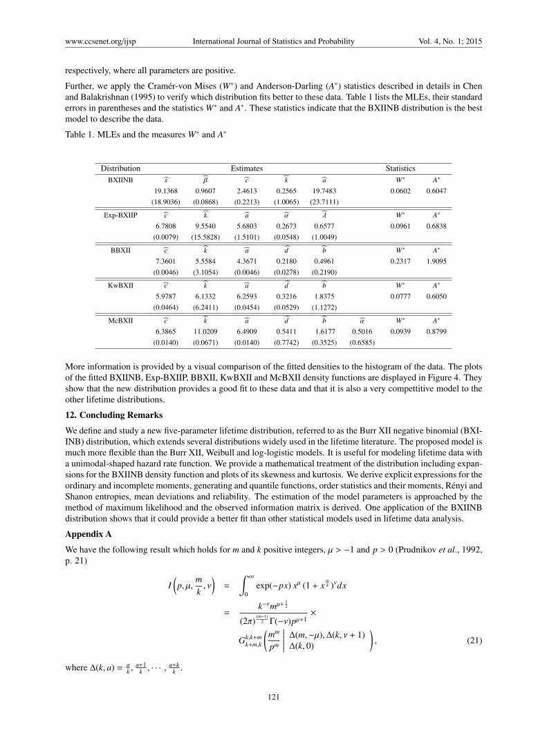
Further, we apply the Cramer-von Mises (W∗) and Anderson-Darling (A∗) statistics described in details in Chenand Balakrishnan (1995) to verify which distribution fits better to these data. Table 1 lists the MLEs, their standarderrors in parentheses and the statistics W∗ and A∗. These statistics indicate that the BXIINB distribution is the bestmodel to describe the data.

Table 1. MLEs and the measures W∗ and A∗

Distribution Estimates StatisticsBXIINB s β c k a W∗ A∗

19.1368 0.9607 2.4613 0.2565 19.7483 0.0602 0.6047(18.9036) (0.0868) (0.2213) (1.0065) (23.7111)

Exp-BXIIP c k a α λ W∗ A∗

6.7808 9.5540 5.6803 0.2673 0.6577 0.0961 0.6838(0.0079) (15.5828) (1.5101) (0.0548) (1.0049)

BBXII c k a d b W∗ A∗

7.3601 5.5584 4.3671 0.2180 0.4961 0.2317 1.9095(0.0046) (3.1054) (0.0046) (0.0278) (0.2190)

KwBXII c k a d b W∗ A∗

5.9787 6.1332 6.2593 0.3216 1.8375 0.0777 0.6050(0.0464) (6.2411) (0.0454) (0.0529) (1.1272)

McBXII c k a d b α W∗ A∗

6.3865 11.0209 6.4909 0.5411 1.6177 0.5016 0.0939 0.8799(0.0140) (0.0671) (0.0140) (0.7742) (0.3525) (0.6585)

More information is provided by a visual comparison of the fitted densities to the histogram of the data. The plotsof the fitted BXIINB, Exp-BXIIP, BBXII, KwBXII and McBXII density functions are displayed in Figure 4. Theyshow that the new distribution provides a good fit to these data and that it is also a very compettitive model to theother lifetime distributions.

12. Concluding Remarks

We define and study a new five-parameter lifetime distribution, referred to as the Burr XII negative binomial (BXI-INB) distribution, which extends several distributions widely used in the lifetime literature. The proposed model ismuch more flexible than the Burr XII, Weibull and log-logistic models. It is useful for modeling lifetime data witha unimodal-shaped hazard rate function. We provide a mathematical treatment of the distribution including expan-sions for the BXIINB density function and plots of its skewness and kurtosis. We derive explicit expressions for theordinary and incomplete moments, generating and quantile functions, order statistics and their moments, Renyi andShanon entropies, mean deviations and reliability. The estimation of the model parameters is approached by themethod of maximum likelihood and the observed information matrix is derived. One application of the BXIINBdistribution shows that it could provide a better fit than other statistical models used in lifetime data analysis.

Appendix A

We have the following result which holds for m and k positive integers, µ > −1 and p > 0 (Prudnikov et al., 1992,p. 21)

I(p, µ,

mk, ν

)=

∫ ∞

0exp(−px) xµ (1 + x

mk )νdx

=k−νmµ+ 1

2

(2π)(m−1)

2 Γ(−ν)pµ+1×

Gk,k+mk+m,k

(mm

pm

∣∣∣∣∣∣ ∆(m,−µ),∆(k, ν + 1)∆(k, 0)

), (21)

where ∆(k, a) = ak ,

a+1k , · · · , a+k

k .

121


x

Den

sity

0 1 2 3 4 5 6 7

0.0

0.1

0.2

0.3

0.4

0.5

BXIINBExp−BXIIPBBXIIKwBXIIMcBXII

Figure 4. Some fitted densities to the histogram of the current data.

Appendix B

Uss = −n{[

(1 − β)s − 1]2 − s2(1 − β)s log2(1 − β)

}s2 [

(1 − β)s − 1]2 ,

Usβ =n[1 − (1 − β)s + s(1 − β)s log(1 − β)

](β − 1)

[(1 − β)s − 1

]2 +

n∑i=1

[1 +

(xia

)c]−k

1 − β[1 +

(xia

)c]−k ,

Usc = −n∑

i=1

βk(

xia

)c log

(xia

) [1 +

(xia

)c]−k−1

1 − β[1 +

(xia

)c]−k ,

Usk = −n∑

i=1

β[1 +

(xia

)c]−klog

[1 +

(xia

)c]1 − β

[1 +

(xia

)c]−k ,

Usa =

n∑i=1

β c k xi

(xia

)c−1 [1 +

(xia

)c]−k−1

a2{1 − β

[1 +

(xia

)c]−k} ,

Uββ = n

s[s(1 − β)s + (1 − β)s − 1

](β − 1)2 [

(1 − β)s − 1]2 − 1

β2

+ (s + 1)n∑

i=1

[1 +

(xia

)c]−2k

{1 − β

[1 +

(xia

)c]−k}2 ,

122


Uβc = −(s + 1)n∑

i=1

k(

xia

)clog

(xia

) [1 +

(xia

)c]−k−1

1 − β[1 +

(xia

)c]−k +β k

(xia

)clog

(xia

) [1 +

(xia

)c]−2k−1

{1 − β

[1 +

(xia

)c]−k}2

,

Uβk = −(s + 1)n∑

i=1

β[1 +

(xia

)c]−2klog

[1 +

(xia

)c]{1 − β

[1 +

(xia

)c]−k}2 +

[1 +

(xia

)c]−klog

[1 +

(xia

)c]1 − β

[1 +

(xia

)c]−k

,

Uβa = (s + 1)n∑

i=1

c k xi

(xia

)c−1 [1 +

(xia

)c]−k−1

a2{1 − β

[1 +

(xia

)c]−k} +β c k xi

(xia

)c−1 [1 +

(xia

)c]−2k−1

a2{1 − β

[1 +

(xia

)c]−k}2

,

Ucc =nc2 + (s + 1)

[ n∑i=1

(β2k2(

xia

)2clog2

(xia

) [1 +

(xia

)c]−2k−2

{1 − β

[1 +

(xia

)c]−k}2 −β k

(xia

)clog2

(xia

)1 − β

[1 +

(xia

)c]−k

×[1 +

( xi

a

)c]−k−1−β k(−k − 1)

(xia

)2clog2

(xia

) [1 +

(xia

)c]−k−2

1 − β[1 +

(xia

)c]−k

)]

+(k + 1)[ n∑

i=1

( ( xia

)clog2

(xia

)1 +

(xia

)c −

(xia

)2clog2

(xia

)[1 +

(xia

)c]2

)],

Uck = −n∑i

(xia

)clog

(xia

)1 +

(xia

)c + (s + 1)n∑

i=1

(β2k(

xia

)clog

(xia

)log

[1 +

(xia

)c]{1 − β

[1 +

(xia

)c]−k}2

×[1 +

( xi

a

)c]−2k−1−β(

xia

)clog

(xia

) [1 +

(xia

)c]−k−1

1 − β[1 +

(xia

)c]−k +β k

(xia

)c log

(xia

)1 − β

[1 +

(xia

)c]−k

×[1 +

( xi

a

)c]−k−1log

[1 +

( xi

a

)c] ),

Uca = −(s + 1)n∑

i=1

(β2c k2xi

(xia

)2c−1log

(xia

) [1 +

(xia

)c]−2k−2

a2{1 − β

[1 +

(xia

)c]−k}2 −β c k xi

(xia

)c−1{1 − β

[1 +

(xia

)c]−k}× 1

a2 log( xi

a

) [1 +

( xi

a

)c]−k−1−β c (−k − 1) k xi

(xia

)2c−1log

(xia

) [1 +

(xia

)c]−k−2

a2{1 − β

[1 +

(xia

)c]−k}−β k

(xia

)c [1 +

(xia

)c]−k−1

a{1 − β

[1 +

(xia

)c]−k} )− (k + 1)

n∑i

{c xi

(xia

)c−1 log

(xia

)a2

[1 +

(xia

)c] +

(xia

)c

a[1 +

(xia

)c]−

c xi

(xia

)2c−1log

(xia

)a2

[1 +

(xia

)c]2

}+

na,

123


Ukk = − nk2 + (s + 1)

n∑i=1

(β2[1 +

(xia

)c]−2klog2

[1 +

(xia

)c]{1 − β

[1 +

(xia

)c]−k}2 +β[1 +

(xia

)c]−k

1 − β[1 +

(xia

)c]−k

× log2[1 +

( xi

a

)c] ),

Uka =

n∑i=1

c xi

(xia

)c−1

a2[1 +

(xia

)c] − (s + 1)n∑

i=1

(β2c k xi

(xia

)c−1 [1 +

(xia

)c]−2k−1log

[1 +

(xia

)c]a2

{1 − β

[1 +

(xia

)c]−k}2

−β c xi

(xia

)c−1 [1 +

(xia

)c]−k−1

a2{1 − β

[1 +

(xia

)c]−k} +β c k xi

(xia

)c−1 [1 +

(xia

)c]−k−1log

[1 +

(xia

)c]a2

{1 − β

[1 +

(xia

)c]−k} ),

Uaa =c na2 − (s + 1)

n∑i=1

(−β2c2k2x2

i

(xia

)2c−2 [1 +

(xia

)c]−2k−2

a4{1 − β

[1 +

(xia

)c]−k}2 +β c2 (−k − 1) k{

1 − β[1 +

(xia

)c]−k}×

x2i

a4

( xi

a

)2c−2 [1 +

( xi

a

)c]−k−2+β c k (c − 1) x2

i

(xia

)c−2 [1 +

(xia

)c]−k−1

a4{1 − β

[1 +

(xia

)c]−k}+

2β c k xi

(xia

)c−1 [1 +

(xia

)c]−k−1

a3{1 − β

[1 +

(xia

)c]−k} )+ (k + 1)

n∑i=1

( c2x2i

(xia

)2c−2

a4[1 +

(xia

)c]2 −c (c − 1)[1 +

(xia

)c]×

x2i

a4

( xi

a

)c−2−

2cxi

(xia

)c−1

a3[1 +

(xia

)c] ).References

Chen, G., & Balakrishnan, N. (1995). A general purpose approximate goodness-of-fit test. Journal of QualityTechnology, 27, 154–161.

Doornik, J. A. (2006). An Object-Oriented Matrix Language-Ox 4, 5th ed. Timberlake Consultants Press: London.

Gradshteyn, I. S., & Ryzhik, I. M. (2000). Table of Integrals, Series and Products. Academic Press, San Diego.

Kenney, J. F., & Keeping, E. S. (1962). Mathematics of Statistics, Part 1, 3rd ed. Princeton, New Jersey.

Moors, J. J. (1988). A quantile alternative for kurtosis. Journal of the Royal Statistical Society D, 37, 25–32.

Murthy, D. N. P., Xie, M., & Jiang, R. (2004). Weibull Models, John Wiley and Sons, New Jersey.

Parnaiba, P. F. P., Ortega, E. M. M., Cordeiro, G. M., & Pescim, R. R. (2011). The beta Burr XII distribution withapplication to lifetime data. Computational Statistics and Data Analysis, 55, 1118–1136.http://dx.doi.org/10.1016/j.csda.2010.09.009

Parnaiba, P. F. P., Ortega, E. M. M., Cordeiro, G. M., & Pascoa, M. A. R. (2012). The Kumaraswamy Burr XIIdistribution: Theory and Practice. Journal of Statistical Computation and Simulation, 82, 1–27.

Percontini, A., Cordeiro, G. M., & Bourguignon, M. (2013). The G-Negative Binomial Family: General Propertiesand Applications. Advances and Applications in Statistics, 35, 127–160.

Prudnikov, A. P., Brychkov, Y. A., & Marichev, O. I. (1986). Integrals and Series, volume 1. Gordon and BreachScience Publishers, Amsterdam.

124


Prudnikov, A. P., Brychkov, Y. A., & Marichev, O. I. (1992). Integrals and Series, volume 4. Gordon and BreachScience Publishers, Amsterdam.

Renyi, A. (1961). On measures of entropy and information. In: Proceedings of the 4th Berkeley Symposium onMathematical Statistics and Probability, I, 547-561. University of California Press: Berkeley.

Shannon, C. E. (1951). Prediction and entropy of printed English. The Bell System Technical Journal, 30, 50-64.http://dx.doi.org/10.1002/j.1538-7305.1951.tb01366.x

Shao, Q. (2004a). Notes on maximum likelihood estimation for the three-parameter Burr XII distribution. Com-putational Statistics and Data Analysis, 45, 675–687. http://dx.doi.org/10.1016/S0167-9473(02)00367-5

Shao, Q., Wong, H., & Xia, J. (2004b). Models for extremes using the extended three parameter Burr XII systemwith application to flood frequency analysis. Hydrological Sciences (Journal des Sciences Hydrologiques),49, 685–702. http://dx.doi.org/10.1623/hysj.49.4.685.54425

Silva, G. O., Ortega, E. M. M., Garibay, V. C., & Barreto, M. L. (2008). Log-Burr XII regression models withcensored Data. Computational Statistics and Data Analysis, 52, 3820–3842.http://dx.doi.org/10.1016/j.csda.2008.01.003

Silva, G. O., Ortega, E. M. M., & Paula, G. A. (2011). Residuals for log-Burr XII regression models in survivalanalysis. Journal of Applied Statistics, 38, 1435–1445. http://dx.doi.org/10.1080/02664763.2010.505950

Soliman, A. A. (2005). Estimation of Parameters of Life from Progressively Censored Data using Burr-XII Model.IEEE Transactions on Reliability, 54, 34–42. http://dx.doi.org/10.1109/TR.2004.842528

Wu, S. J., Chen, Y. J., & Chang, C. T. (2007). Statistical inference based on progressively censored samples withrandom removals from the Burr type XII distribution. Journal of Statistical Computation and Simulation, 77,19–27. http://dx.doi.org/10.1080/10629360600569204

Zimmer, W. J., Keats, J. B., & Wang, F. K. (1998). The Burr XII distribution in reliability analysis. Journal ofQuality Technology, 30, 386–94.

Copyrights

Copyright for this article is retained by the author(s), with first publication rights granted to the journal.

This is an open-access article distributed under the terms and conditions of the Creative Commons Attributionlicense (http://creativecommons.org/licenses/by/3.0/).

125

The Burr XII Negative Binomial Distribution with Applications to Lifetime Data

Documents

Transcript of The Burr XII Negative Binomial Distribution with Applications to Lifetime Data