Customer Lifetime Value for Retail Based on Transactional ...

UKRAINIAN CATHOLIC UNIVERSITY

MASTER THESIS

Customer Lifetime Value for Retail Basedon Transactional and Loyalty Card Data

Author:Anastasiia KASPROVA

Supervisor:Liubomyr BREGMAN

A thesis submitted in fulfillment of the requirementsfor the degree of Master of Science

in the

Department of Computer SciencesFaculty of Applied Sciences

Lviv 2020

http://www.ucu.edu.ua

http://www.johnsmith.com

http://www.jamessmith.com

http://researchgroup.university.com

http://department.university.com

i

Declaration of AuthorshipI, Anastasiia KASPROVA, declare that this thesis titled, “Customer Lifetime Value forRetail Based on Transactional and Loyalty Card Data” and the work presented in itare my own. I confirm that:

• This work was done wholly or mainly while in candidature for a research de-gree at this University.

• Where any part of this thesis has previously been submitted for a degree orany other qualification at this University or any other institution, this has beenclearly stated.

• Where I have consulted the published work of others, this is always clearlyattributed.

• Where I have quoted from the work of others, the source is always given. Withthe exception of such quotations, this thesis is entirely my own work.

• I have acknowledged all main sources of help.

• Where the thesis is based on work done by myself jointly with others, I havemade clear exactly what was done by others and what I have contributed my-self.

Signed:

Date:

ii

“Fit fabricando faber.”

iii

UKRAINIAN CATHOLIC UNIVERSITY

Faculty of Applied Sciences

Master of Science

Customer Lifetime Value for Retail Based on Transactional and Loyalty CardData

by Anastasiia KASPROVA

Abstract

The modeling of CLV in retail is a complicated task due to the lack of access tohistorical data of purchases, the difficulty of customer identification, and buildingthe historical reference with a particular customer.

In this research, historical transactional data were taken from twelve North Amer-ican brick-and-mortar grocery stores to compare different approaches to CLV mod-eling in terms of segmentation and forecast. Data engineering pipeline was appliedto raw transactional data to transfer it into ready-for-modeling datasets, providingwith the logic of each obtained feature. K-Means, Gaussian Mixture Model (GMM),DBSCAN clustering algorithms were applied to customer segmentation. The bestoutputs of clustering samples were later tested in CLV modeling. Unexpectedly, theK-Means algorithm results overperformed both GMM and DBSCAN ones.

For CLV modeling, two main models were considered: Markov Chain proba-bilistic approach of changing purchase behavior over time alongside with econo-metric Time Series revenue forecast and Survival Analytics lifespan estimates. Thesuggestions on CLV estimation for the offline retail business case were derived afterresult comparison with given advantages and limitations of each approach. MarkovChain model was suggested to check the general picture of the ongoing processesfrom the long-term perspective. On the other hand, Time Series revenue forecastingwith Survival Analytics lifespan estimates could be used to check the expectationsfor the nearest feature. Moreover, the business value of CLV estimates and its appli-cations were shown on examples derived from the results of both models: definedthe promising clusters, checked their stability, and how they were formed, what cus-tomers were at risk to churn.

HTTP://WWW.UCU.EDU.UA

http://department.university.com

iv

AcknowledgementsI want to express my special thanks of gratitude to Liubomyr Bregman for the su-pervision, all the support throughout the research, and hours spent on knowledgesharing and valuable feedbacks. I want to thank Dima Fishman, Sergii Shelpuk, andOleksandr Romanko. I do appreciate your impact on my professional developmentchoice. My special thanks go to Oleksii Molchanovskyi for the excellent quality Mas-ter Program in Data Science he has created at the Ukrainian Catholic University. Ifeel so lucky to know you in person and do value your humanity and professionalqualities. I am incredibly thankful to Dmitry Leader and Grammarly Inc. for provid-ing me with a scholarship to partly cover my tuition fees and reach the Dream muchcomfortable. And of course, I express my deepest gratitude to my parents who al-ways support me with any idea or aspiration I have and to my son who alwaysinspires me to Dream Big and Live in Wonders.

v

Contents

Declaration of Authorship i

Abstract iii

Acknowledgements iv

1 Introduction 11.1 Importance of CLV . . . . . . . . . . . . . . . . . . . . . . . . . . . . . . 11.2 Challenges of CLV modeling for offline retail business . . . . . . . . . . 11.3 Goals of the master thesis . . . . . . . . . . . . . . . . . . . . . . . . . . 21.4 Thesis Structure . . . . . . . . . . . . . . . . . . . . . . . . . . . . . . . . 2

2 Overview of existing approaches 32.1 CLV Models Classification . . . . . . . . . . . . . . . . . . . . . . . . . . 3

2.1.1 Deterministic Approach . . . . . . . . . . . . . . . . . . . . . . . 3RFM . . . . . . . . . . . . . . . . . . . . . . . . . . . . . . . . . . 4

2.1.2 Stochastic Approach . . . . . . . . . . . . . . . . . . . . . . . . . 4Probability models . . . . . . . . . . . . . . . . . . . . . . . . . . 4Econometric models . . . . . . . . . . . . . . . . . . . . . . . . . 4Computer Science models . . . . . . . . . . . . . . . . . . . . . . 5

2.2 Customer segmentation . . . . . . . . . . . . . . . . . . . . . . . . . . . 5

3 Proposed models 63.1 Clustering Algorithms . . . . . . . . . . . . . . . . . . . . . . . . . . . . 7

3.1.1 K-Means . . . . . . . . . . . . . . . . . . . . . . . . . . . . . . . . 73.1.2 Gaussian Mixture Model . . . . . . . . . . . . . . . . . . . . . . . 83.1.3 DBSCAN . . . . . . . . . . . . . . . . . . . . . . . . . . . . . . . . 93.1.4 Summary . . . . . . . . . . . . . . . . . . . . . . . . . . . . . . . 11

3.2 Markov Chain . . . . . . . . . . . . . . . . . . . . . . . . . . . . . . . . . 113.3 Survival Analysis . . . . . . . . . . . . . . . . . . . . . . . . . . . . . . . 11

3.3.1 Kaplan-Meier Survival Curves . . . . . . . . . . . . . . . . . . . 123.3.2 Cox’s Proportional Hazard Model . . . . . . . . . . . . . . . . . 13

3.4 Time Series . . . . . . . . . . . . . . . . . . . . . . . . . . . . . . . . . . . 133.4.1 ARIMA, SARIMA . . . . . . . . . . . . . . . . . . . . . . . . . . 133.4.2 LSTM . . . . . . . . . . . . . . . . . . . . . . . . . . . . . . . . . . 14

3.5 CLV calculation . . . . . . . . . . . . . . . . . . . . . . . . . . . . . . . . 153.6 Summary . . . . . . . . . . . . . . . . . . . . . . . . . . . . . . . . . . . . 15

4 Datasets Preparation 164.1 Raw Data Description . . . . . . . . . . . . . . . . . . . . . . . . . . . . 164.2 Data Cleaning . . . . . . . . . . . . . . . . . . . . . . . . . . . . . . . . . 164.3 Feature generation . . . . . . . . . . . . . . . . . . . . . . . . . . . . . . 17

4.3.1 Clustering . . . . . . . . . . . . . . . . . . . . . . . . . . . . . . . 17

vi

4.3.2 Survival Analytics . . . . . . . . . . . . . . . . . . . . . . . . . . 174.3.3 Time Series . . . . . . . . . . . . . . . . . . . . . . . . . . . . . . 17

4.4 Data Preprocessing . . . . . . . . . . . . . . . . . . . . . . . . . . . . . . 184.5 Dimensionality Reduction . . . . . . . . . . . . . . . . . . . . . . . . . . 184.6 Summary . . . . . . . . . . . . . . . . . . . . . . . . . . . . . . . . . . . . 18

5 Experiments 205.1 Analytical Environment . . . . . . . . . . . . . . . . . . . . . . . . . . . 205.2 Clusterization . . . . . . . . . . . . . . . . . . . . . . . . . . . . . . . . . 20

5.2.1 K-Means . . . . . . . . . . . . . . . . . . . . . . . . . . . . . . . . 20Elbow Method . . . . . . . . . . . . . . . . . . . . . . . . . . . . 20Silhouette Score . . . . . . . . . . . . . . . . . . . . . . . . . . . . 21

5.2.2 Gaussian Mixture Model . . . . . . . . . . . . . . . . . . . . . . . 225.2.3 DBSCAN . . . . . . . . . . . . . . . . . . . . . . . . . . . . . . . . 235.2.4 Summary . . . . . . . . . . . . . . . . . . . . . . . . . . . . . . . 25

5.3 Markov Chain . . . . . . . . . . . . . . . . . . . . . . . . . . . . . . . . . 255.3.1 CLV modeling . . . . . . . . . . . . . . . . . . . . . . . . . . . . . 255.3.2 Model evaluation . . . . . . . . . . . . . . . . . . . . . . . . . . . 255.3.3 Business Value vs CLV forecast . . . . . . . . . . . . . . . . . . . 275.3.4 Summary . . . . . . . . . . . . . . . . . . . . . . . . . . . . . . . 28

5.4 Survival Analytics . . . . . . . . . . . . . . . . . . . . . . . . . . . . . . . 285.4.1 Cox’s Proportional Hazard Model . . . . . . . . . . . . . . . . . 285.4.2 Accuracy and calibration of CPH model . . . . . . . . . . . . . . 295.4.3 CPH CLV Benchmark model . . . . . . . . . . . . . . . . . . . . 295.4.4 Summary . . . . . . . . . . . . . . . . . . . . . . . . . . . . . . . 31

5.5 Time Series Forecasting . . . . . . . . . . . . . . . . . . . . . . . . . . . . 315.5.1 Weekly Time Series on Cluster Level . . . . . . . . . . . . . . . . 325.5.2 Business Value vs CLV forecast . . . . . . . . . . . . . . . . . . . 335.5.3 Summary . . . . . . . . . . . . . . . . . . . . . . . . . . . . . . . 34

5.6 Summary . . . . . . . . . . . . . . . . . . . . . . . . . . . . . . . . . . . . 35

6 Conclusions and Future Work 366.1 Conclusions . . . . . . . . . . . . . . . . . . . . . . . . . . . . . . . . . . 366.2 Future Work . . . . . . . . . . . . . . . . . . . . . . . . . . . . . . . . . . 36

Bibliography 38

vii

List of Figures

2.1 CLV models classification defined by Gupta et al., 2006. Source: Author 3

3.1 Pipeline of a probabilistic approach with Markov Chain CLV predic-tion. Source: Author. . . . . . . . . . . . . . . . . . . . . . . . . . . . . . 6

3.2 Pipeline of the econometric approach of CLV prediction. Source: Au-thor. . . . . . . . . . . . . . . . . . . . . . . . . . . . . . . . . . . . . . . . 7

3.3 Illustration of K-Means clustering steps. Source: K-Means and X-MeansClustering. . . . . . . . . . . . . . . . . . . . . . . . . . . . . . . . . . . . 8

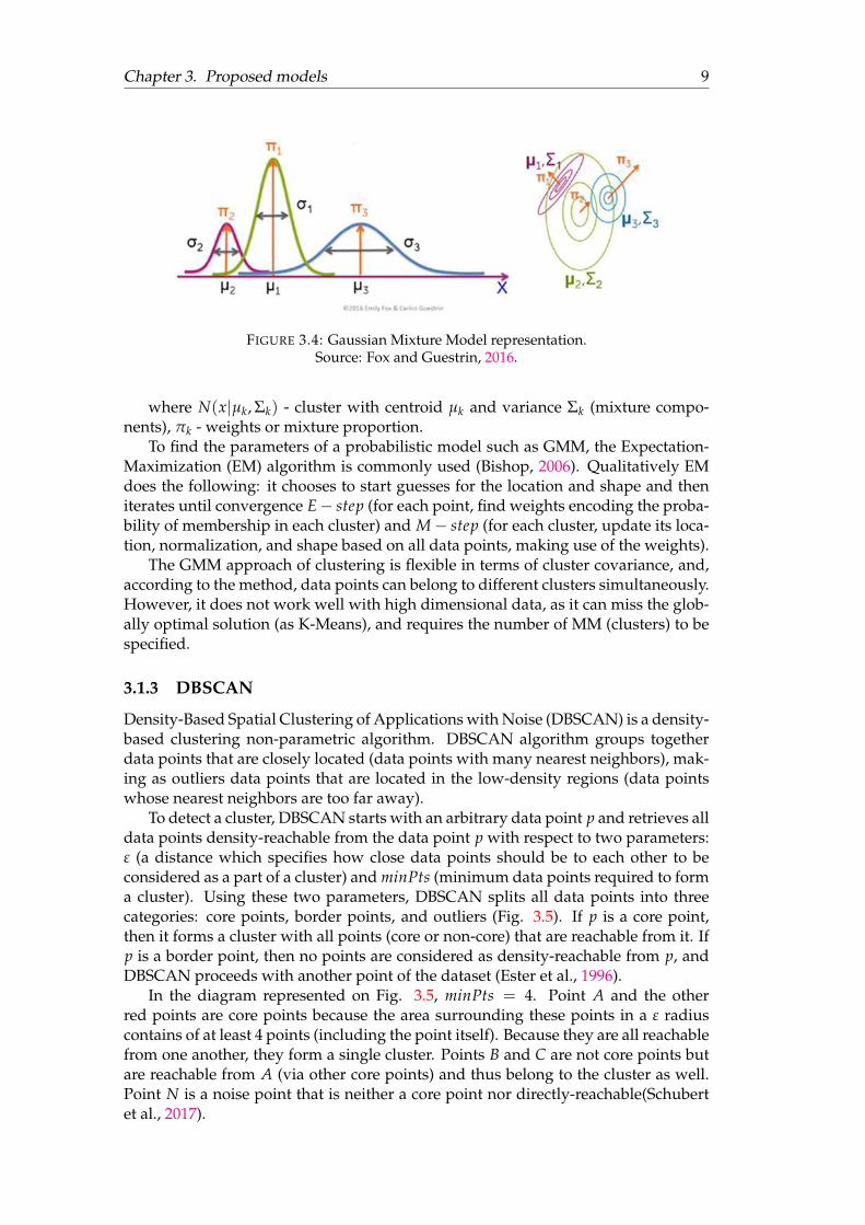
3.4 Gaussian Mixture Model representation. Source: Fox and Guestrin,2016. . . . . . . . . . . . . . . . . . . . . . . . . . . . . . . . . . . . . . . 9

3.5 DBSCAN slit explanation. Source: Schubert et al., 2017. . . . . . . . . . 103.6 Comparison of K-Means, DBSCAN and GMM clustering algorithms

on 2D data. Source: Overview of clustering methods. . . . . . . . . . . . . 103.7 Example of the transition graph between segment 1 and segment 2.

Source: Author. . . . . . . . . . . . . . . . . . . . . . . . . . . . . . . . . 113.8 Survival curve estimated by Kaplan-Meier model. Source: Author. . . 123.9 Repeating module in LSTM. Source: Mittal, 2019. . . . . . . . . . . . . . 14

4.1 General dataset preparation pipeline. Source: Author. . . . . . . . . . . 164.2 Feature Matrix Correlation. Source: Author. . . . . . . . . . . . . . . . . 18

5.1 Dependence of Within Cluster Sum of Squares (or K-Means score) onthe number of clusters (Elbow Method). Source: Author. . . . . . . . . 21

5.2 Dependence of silhouette score on the number of clusters (K-Means).Source: Author. . . . . . . . . . . . . . . . . . . . . . . . . . . . . . . . . 21

5.3 Histograms of customer distribution within 17(A), 20(B), and 21 (C)clusters (K-Means). Source: Author. . . . . . . . . . . . . . . . . . . . . 22

5.4 Dependence of silhouette score on the number of clusters (GMM).Source: Author. . . . . . . . . . . . . . . . . . . . . . . . . . . . . . . . . 22

5.5 Histograms of customer distribution within 8 (A), 11 (B), 17 (C), 20(D), 21 (E) clusters (GMM). Source: Author. . . . . . . . . . . . . . . . . 23

5.6 The Elbow method to find ε value for DBSCAN. Source: Author. . . . . 245.7 Histograms of customer distribution within 8 clusters (DBSCAN). Source:

Author. . . . . . . . . . . . . . . . . . . . . . . . . . . . . . . . . . . . . . 245.8 A sample of a Transition Matrix: probability to switch the cluster in

the next month (21-clusters, K-Means). Source: Author. . . . . . . . . . 265.9 A sample of revenue estimation for the next 8 months (21-clusters,

K-Means). Source: Author. . . . . . . . . . . . . . . . . . . . . . . . . . . 265.10 A sample of actual Revenue (ground truth for 21-clusters, K-Means).

Source: Author. . . . . . . . . . . . . . . . . . . . . . . . . . . . . . . . . 275.11 A sample of Sankey diagram of customer transitions between clusters.

Source: Author. . . . . . . . . . . . . . . . . . . . . . . . . . . . . . . . . 275.12 Average predicted CLV vs Current Revenue. Source: Author. . . . . . . 28

viii

5.13 The time dependence of the probability to survive. Source: Author. . . 295.14 Cox’s Proportional Hazard model summary. Source: Author. . . . . . . 305.15 Cox’s Proportional Hazard Model calibration loss over lifespan. Source:

Author. . . . . . . . . . . . . . . . . . . . . . . . . . . . . . . . . . . . . . 305.16 Example of Calibration plots for the lifespan of 100 (A) and 450 (B)

days. Source: Author. . . . . . . . . . . . . . . . . . . . . . . . . . . . . . 315.17 Customer distribution by lifespan: actual versus predicted. Source:

Author. . . . . . . . . . . . . . . . . . . . . . . . . . . . . . . . . . . . . . 315.18 Revenue from a randomly chosen household with daily (A) and weekly

(B) aggregations. Source: Author. . . . . . . . . . . . . . . . . . . . . . . 325.19 Revenue Time Series of the 9th cluster. Source: Author. . . . . . . . . . 325.20 Actual vs Forecasted Revenue of the 9th cluster and model error anal-

ysis. Source: Author. . . . . . . . . . . . . . . . . . . . . . . . . . . . . . 335.21 Average revenue per customer of the 9th cluster. Source: Author. . . . 345.22 Probability to survive for the households of the 9th cluster: general

and at the point of lifespan prediction. Source: Author. . . . . . . . . . 34

ix

List of Tables

5.1 Comparison of Markov Chain RMSE of CLV for different clusteringtechniques. . . . . . . . . . . . . . . . . . . . . . . . . . . . . . . . . . . . 26

x

List of Abbreviations

CLV Customer Lifetime ValueCE Customer EquityCRM Customer Relationship ManagementNDA Non-Disclosure AgreementID Identification NumberUPC Universal Product CodeKNN K-Nearest NeighborsDBSCAN Density-Based Spatal Clustering of Applications with NoiseEM Expectation MinimizationGMM Gaussian Mixture ModelMM Mixture ModelARIMA Auto Regressive Integrated Moving AverageSARIMA Seasonal Auto Regressive Integrated Moving AverageARIMAX Auto Regressive Integrated Moving Average with eXogenous variablesSARIMAX Seasonal Auto Regressive Integrated Moving Average with eXogenous variablesVAR Vector AutoRegressiveVARMAX Vector Autoregression Moving Average with eXogenous variablesLSTM Long Short-Term MemoryCPH Cox’s Proportional HazardRFM Recency Frequency Monetary valueRNN Reccurent Neural NetworkES-RNN Exponential Smoothing-Recurrent Neural NetworksGPU Graphics Proccesing UnitWCSS Within Cluster Sum of SquaresRMSE Root Mean Sum of SquaresAIC Akaike Information CriterionADF Augmented Dickey–Fuller testACF AutoCorrelation FunctionPACF Partial AutoCorrelation FunctionSVM Support Vector MachinesCART Classification And Regression TreesNBD Negative Binomial DistributionMARS Multivariate Adaptive Regression SplinesGAM Generalized Additive Model

xi

Dedicated to my lovely family

1

Chapter 1

Introduction

1.1 Importance of CLV

CLV estimation helps management of a retail company with making data-driven de-cisions in the following areas (Villanueva and Hanssens, 2007, Jasek et al., 2018, Jaseket al., 2019): resources allocation and marketing strategies formulation, customersegmentation to build long-term relationships with clients, effective management ofmarketing investments, retaining and acquiring customers, estimation of companyvalue and evaluation of marketing channels and campaigns.

According to Gupta et al., 2006, companies such as IBM, Capital One, LL Bean,ING, and others use CLV in managing and measuring their business success. Thefollowing factors cause their interest in CLV. (1) First of all, marketing metrics suchas brand awareness, attitudes, sales, and share are not enough to represent the re-turn on marketing investment. Marketing campaigns that improve sales or sharecan negatively impact a long-term profitability of a company. (2) Secondly, financialmetrics such as stock price and aggregated profit of a company are restricted witha diagnostic capability. Aggregated financial metrics cannot catch unprofitable cus-tomers to allocate resources appropriately. (3) Development of IT enables companiesto collect customer transactions easily, build and analyze models, convert data intoinsights, and customize marketing programs for individual customers.

1.2 Challenges of CLV modeling for offline retail business

CLV in offline retail business faces two significant challenges: customer identifica-tion to build the historical reference with a particular customer and a lack of publiclyavailable transactional datasets to validate theoretical aspects of CLV modeling.

According to Jasek et al., 2018, Jasek et al., 2019, there is a number of paperscovering theory of CLV modeling, but there are few of them dedicated to empiricalanalyses, and only a few (Batislam and Filiztekin, 2007, Nikkhahan, Habibi, andTarokh, 2011, Jasek et al., 2018, and Jasek et al., 2019) used real transactional data intheir research. Besides, blogs and tutorials (Medium, TowardsDataScience, etc.) oronline courses (datacamp, coursera, edx, udemy) dedicated to customer analytics,mostly re-use the same datasets (for instance, Online Retail Dataset is often used forRFM analysis explanation, Iris Dataset – clustering, Telco – churn prediction, Titanic– survival analytics). The reason is that most research results in the retail field havea proprietary nature. Retailers rarely reveal results of their investigations to publicaccess to stay on the top of the global market.

In the study, I have used new transactional and loyalty card data taken from theoffline retail business. Having raw data, I have prepared different datasets according

Chapter 1. Introduction 2

to appropriate model requirements and demonstrated the most popular approachesof CLV modeling with it.

1.3 Goals of the master thesis

The practical goal of the project is to create an applicable analytical framework foroffline and semi offline businesses to run CLV forecast for channels and campaignevaluations. The pre-requirement is to have transactional data of purchases, with aselection of suitable for offline retail environment CLV model application based ontransactional and loyalty card data.

According to the goal, there are three main tasks to solve:I. Investigate existing approaches to CLV modeling suitable for the offline retail

business.II. Develop a two-component CLV model: cluster customers and predict revenue

relevant to the cluster of interest based on available transactional and loyalty carddata.

III. Compare models based on their assumption limitations and advantages foran offline store environment.

1.4 Thesis Structure

Firstly, a classification of CLV estimation approaches is introduced in Chapter 2.Then, in Chapter 3, two approaches for CLV modeling and background informa-tion, that makes the basis of proposed methods, are considered. In Chapter 4, eachcomponent of the data engineering pipeline of dataset preparation is described. InChapter 5 the environment where all the experimental work was conducted and theresults of proposed models are represented and discussed. Finally, in Chapter 6, thesuggestions on CLV estimation for the offline retail business case and a list of thedirections of possible future work are represented.

3

Chapter 2

Overview of existing approaches

According to McKinsey, Customer Lifecycle Management, Customer Lifetime Value(CLV) analysis provides a 360-degree view of customers and is used as a tool for avalue maximization on customer level increase in the revenue of a company. Kotler,1974 defined CLV as “present value of the future profit stream expected given atime horizon of transacting with the customer”; however, later, according to Estrella-Ramón et al., 2013, it has studied under different names: Lifetime Value, CustomerEquity, Net Present Value, Customer Profitability, and Customer Value. Various re-searches define CLV slightly differently, but the general idea is that this metric indi-cates the total revenue a company can expect from a single customer to generate overtime. Once it is estimated, it is possible to identify promising customers, minimizeacquisition cost by specific targeting of customers, and organize an efficient CRM(adjust promotions, recommendations, customer service) by prioritizing customers(Machine Learning for Marketing Analytics in R course notes).

2.1 CLV Models Classification

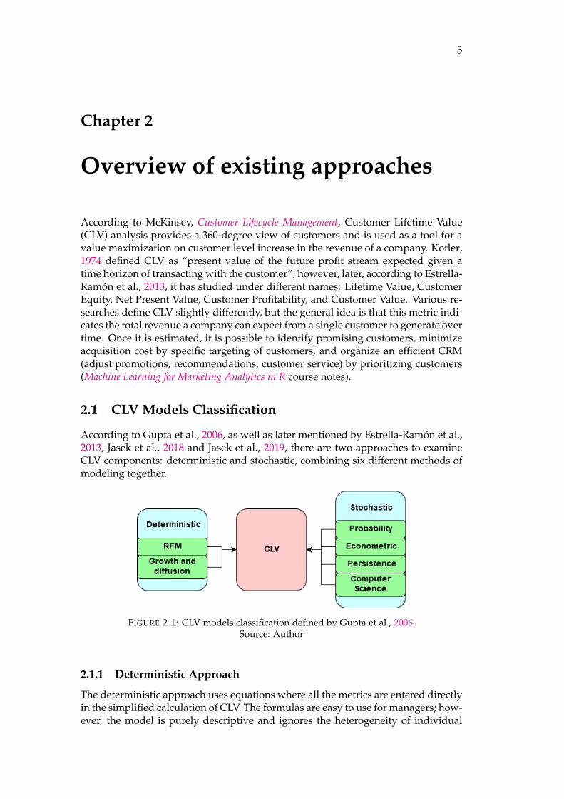
According to Gupta et al., 2006, as well as later mentioned by Estrella-Ramón et al.,2013, Jasek et al., 2018 and Jasek et al., 2019, there are two approaches to examineCLV components: deterministic and stochastic, combining six different methods ofmodeling together.

FIGURE 2.1: CLV models classification defined by Gupta et al., 2006.Source: Author

2.1.1 Deterministic Approach

The deterministic approach uses equations where all the metrics are entered directlyin the simplified calculation of CLV. The formulas are easy to use for managers; how-ever, the model is purely descriptive and ignores the heterogeneity of individual

Chapter 2. Overview of existing approaches 4

customer response probabilities (retention, churn rate within a cohort). The rep-resentatives of this approach are RFM (Recency, Frequency, Monetary value) andGrowth and Diffusion models.

RFM

RFM models have been popular in direct marketing for more than 30 years. Thesemodels were developed to improve response rates by targeting marketing programsat specific customers. Before that, companies used the demography of customers.These models describe customer behavior based on three variables: recency – timesince the last transaction, frequency – number of transactions during a given period,monetary value – the total amount of money spent in transactions during a given pe-riod (Hughes, 2011). The simplest models segment customers based on each valuefor these three variables. More sophisticated models use weights making RFM vari-ables more or less important.

Despite the simplicity of RFM models, they have multiple limitations: the cus-tomer behavior can be predicted only for the next period, a precise description ofthe actual customer behavior cannot be derived from the model variables, othervariables are not taken into account, a monetary amount of customer value is notoffered as a model output. To deal with the disadvantages of the deterministic ap-proach, some researchers advise to mix this approach with stochastic one (RFM withMarkov Chain, for instance, Pfeifer and Carraway, 2000). In the study, RFM variablesare used as input to other models.

2.1.2 Stochastic Approach

The stochastic approach characterizes a sequence of random variables which are in-tegrated into another variable. Each random variable has its probability distributionfunction. The variables can correlate. These CLV models are considered more accu-rate since they take into account customer heterogeneity (retention and churn rate).According to Gupta et al., 2006, Estrella-Ramón et al., 2013, Jasek et al., 2018 andJasek et al., 2019, all stochastic approaches can be divided into probability, econo-metric, persistence, and computer science models.

Probability models

The probability model is a representation of the world where observed behavioris modeled as a stochastic process specified by unobserved/latent behavior, whichdiffers among customers according to some probability distribution. Models thatbelong to this category are Pareto/NBD (Negative Binomial Distribution), Hierar-chical Bayesian, and Markov Chain (Gupta et al., 2006, Estrella-Ramón et al., 2013).In the study, a Markov Chain model to determine the path of a particular customerof switching the clusters over time and then calculate its CLV has used.

Econometric models

Econometric models are similar to probabilistic ones and are widely used in the in-dustry due to their simplicity. These models consist of submodels correspondingto customer acquisition, retention, and expansion (cross-selling and margin), andtheir output later used in CLV estimations. In this work, the focus was on finding aretention component (a probability that a customer stays with a company and per-forms purchasing again). Thus, it has been identified if a customer is still “active”

Chapter 2. Overview of existing approaches 5

(make purchases from a company) and predicted their lifetime duration with a com-pany. Such survival models as Kaplan-Meier survival curves and Cox’s proportionalhazard have been used to estimate time to event of a customer churn from the re-lationship with a company, as well as time series models to estimate the revenue aparticular customer or cluster can bring to the store.

Computer Science models

To computer science models, Gupta et al., 2006 include algorithms of data mining,machine learning, and statistical non-parametric statistics, which use a large num-ber of variables and have high predictive ability. These are projection-pursuit, neu-ral network, decision tree models, spline-based such as generalized additive models(GAM), multivariate adaptive regression splines (MARS), classification and regres-sion trees (CART) and support vector machines (SVM), Random Forest, ExtremeGradient Boosting and other classical Machine Learning Approaches. However, hestates that many of them could be rather suitable for customer churn studies, thanCLV modeling (referring to his shared work with Neslin and Kamakura (Neslin etal., 2006), and points out that these approaches should be studied in future.

Many of the models, developed by scientists decades ago, usually have a differ-ent context for different types of business as well as their investigation was basedon various data sources (database of customers, surveys, public reports, panel data,and managerial judgments, according to Estrella-Ramón et al., 2013). In works ofJasek et al., 2018 and Jasek et al., 2019 it is stated that probability and economet-ric approaches are only suitable for retail business. Thus, for their purposes, theyselect an extended Pareto/NBD model with RFM factors in the computations andMarkov chain model. They do not include diffusion/growth and persistence modelto their research, because these models are not applicable at the level of individualcustomers prediction, but used more in Customer Equity (a long-term value of acompany which is calculating as a sum of CLV of all customers). The authors do notdeal with computer science models as well, mentioning that these models are notenough considered in the literature with a focus on CLV calculations.

2.2 Customer segmentation

In practice, the revenue estimation is rarely done on the individual level due to a lowlevel of accuracy. Instead, data analytics/data scientists usually divide customers bytheir similar purchase behavior into groups (micro-segmentation) and then predictfuture purchases towards a particular segment of customers.

There are multiple both unsupervised and supervised approaches to a customersegmentation described by Wedel and Kamakura, 1999. All of the methods whichbelonged to unsupervised machine learning have no exact answer on how to dividecustomers, and the results of segmentation could vary from approach to approach.In the study, the most common clustering algorithms have been used, particularly K-Means, Density-Based Spatial Clustering (DBSCAN), and Gaussian mixture models(GMM).

6

Chapter 3

Proposed models

The main aim of this study is to build a CLV model based on transactional andloyalty card data. To achieve this goal, different approaches have been examinedand the one, which fits the data best, has been selected:

1. Probabilistic approach with Markov Chain revenue estimation (Fig. 3.1).

FIGURE 3.1: Pipeline of a probabilistic approach with Markov ChainCLV prediction. Source: Author.

In this approach, I prepared a dataset based on 4-weeks analytics of each cus-tomer (see Chapter 4, Dataset Preparation) and clustered customers using K-Means,Gaussian Mixture Model, and DBSCAN clustering algorithms. Then transition ma-trices has been calculated using Markov Chain Model for each of the clustering out-puts. Knowing IDs of households of each cluster, I derived average revenue andaverage retention per cluster. After that I predicted CLV for each cluster for the pe-riod I have been interested in and evaluated those three models on actual historicaldata.

2. Econometric approach with survival analytics lifetime estimation and timeseries revenue prediction (Fig. 3.2).

In this approach, I prepared two datasets separately with weekly aggregationson a customer level for Time Series Forecasting and overall period aggregations forSurvival Analytics. To predict revenue per week on an individual level, I chose thebest Time Series Model from ARIMA/SARIMA and LSTM based on AIC metric. Ichecked the overall customer life duration with a Kaplan-Meier survival curve and

Chapter 3. Proposed models 7

estimate individual lifespan with Cox’ Proportional Hazard Model for each house-hold with a 0.5 threshold. Finally, the outputs of both models have been used tocalculate CLV for each household.

FIGURE 3.2: Pipeline of the econometric approach of CLV prediction.Source: Author.

Once the results of both approaches ware obtained, it became possible to con-clude what method with what data pipeline works best for the data used in the re-search; also, there was one more step added to the econometric approach – mappingcluster IDs to households and month IDs to weeks.

3.1 Clustering Algorithms

Clustering is a process of applying unsupervised Machine Learning algorithms forautomatic grouping of objects where objects within each group (cluster) are moresimilar to each other than objects from different groups. By belongings of data pointsto a cluster, there are two subgroups of clustering that can be considered: hard,when each data point belongs only to one cluster, and soft, when each data point isan assigned probability to be in clusters. By approaches, clustering algorithms canbe divided into four types: centroid, distribution, density, and connectivity mod-els. Bellow, I consider the representatives of the first three groups to check whatapproach works best with the available dataset.

3.1.1 K-Means

K-Means is a centroid-based clustering algorithm, which is based on distance mea-surement between data points and a centroid of the cluster.

The objective function is defined as:

arg mink

∑i=1

∑x∈Si

||x− µ||2 (3.1)

where x – data point of the dataset, µ – cluster mean, S – cluster, k – number ofclusters.

To partition data points into k predefined clusters, K-Means initializes arbitraryk data points – centroids (cluster centers) and assigns each data point to the closest


centroid forming k cluster, measured by Euclidean distance, cosine similarity, etc.Then each cluster center is replaced by the coordinate-wise average of all data pointsthat are the closest to it (Fig. 3.3). Both steps are repeated until convergence. K-Means algorithm converges to a local minimum of the within-cluster sum of squares(Lloyd, 1982).

FIGURE 3.3: Illustration of K-Means clustering steps. Source: K-Means and X-Means Clustering.

The K-Means algorithm is popular due to its computational efficiency and abil-ity to handle large datasets. However, it provides only linear separation of clusterboundaries, expects that the number of clusters is known, does not work with cate-gorical, ordinal or count variables, and not very robust to missing data. It can alsobe hard to maintain over time and replicate the results.

3.1.2 Gaussian Mixture Model

Gaussian mixture model (GMM) is a probabilistic approach of clustering. It uses asoft clustering approach for distributing the points in different clusters.

According to probabilistic interpretation, clustering can be considered as theidentification of components of a probability density function that generated thedata. Similarly, an identification of cluster centroids can be considered as a discoveryof the modes of distribution. Thus, GMM assumes that all the data points are gen-erated from a mixture of a finite number of Gaussian distributions with unknownparameters (Fig. 3.4). Mixture Models can be also considered as a generalization ofK-Means clustering to incorporate the information about the covariance structure ofdata as well as centers of latent Gaussians.

Mathematically a mixture of k Gaussians can be represented by a formula:

p(x) =k

∑i=1

πkN(x|µk, Σk) (3.2)


FIGURE 3.4: Gaussian Mixture Model representation.Source: Fox and Guestrin, 2016.

where N(x|µk, Σk) - cluster with centroid µk and variance Σk (mixture compo-nents), πk - weights or mixture proportion.

To find the parameters of a probabilistic model such as GMM, the Expectation-Maximization (EM) algorithm is commonly used (Bishop, 2006). Qualitatively EMdoes the following: it chooses to start guesses for the location and shape and theniterates until convergence E− step (for each point, find weights encoding the proba-bility of membership in each cluster) and M− step (for each cluster, update its loca-tion, normalization, and shape based on all data points, making use of the weights).

The GMM approach of clustering is flexible in terms of cluster covariance, and,according to the method, data points can belong to different clusters simultaneously.However, it does not work well with high dimensional data, as it can miss the glob-ally optimal solution (as K-Means), and requires the number of MM (clusters) to bespecified.

3.1.3 DBSCAN

Density-Based Spatial Clustering of Applications with Noise (DBSCAN) is a density-based clustering non-parametric algorithm. DBSCAN algorithm groups togetherdata points that are closely located (data points with many nearest neighbors), mak-ing as outliers data points that are located in the low-density regions (data pointswhose nearest neighbors are too far away).

To detect a cluster, DBSCAN starts with an arbitrary data point p and retrieves alldata points density-reachable from the data point p with respect to two parameters:ε (a distance which specifies how close data points should be to each other to beconsidered as a part of a cluster) and minPts (minimum data points required to forma cluster). Using these two parameters, DBSCAN splits all data points into threecategories: core points, border points, and outliers (Fig. 3.5). If p is a core point,then it forms a cluster with all points (core or non-core) that are reachable from it. Ifp is a border point, then no points are considered as density-reachable from p, andDBSCAN proceeds with another point of the dataset (Ester et al., 1996).

In the diagram represented on Fig. 3.5, minPts = 4. Point A and the otherred points are core points because the area surrounding these points in a ε radiuscontains of at least 4 points (including the point itself). Because they are all reachablefrom one another, they form a single cluster. Points B and C are not core points butare reachable from A (via other core points) and thus belong to the cluster as well.Point N is a noise point that is neither a core point nor directly-reachable(Schubertet al., 2017).


FIGURE 3.5: DBSCAN slit explanation. Source: Schubert et al., 2017.

In contrast to K-Means and GMM algorithms, DBSCAN discovers the numberof clusters. It can also detect the outliers, supports a non-linear separation of theclusters and can separate high- and low-density clusters. However, DBSCAN canbe completely inappropriate for certain datasets, because it tends to merge clusterswith overlapping regions. Moreover, it still requires to set up two parameters: ε andminPts.

FIGURE 3.6: Comparison of K-Means, DBSCAN and GMM clusteringalgorithms on 2D data. Source: Overview of clustering methods.

The comparison of the clustering algorithms performance used in the study isrepresented in Fig. 3.6. However, data used for algorithm performance testing hadonly two dimensions.


3.1.4 Summary

There is no such thing as the best clusterization technique. It is considered that thebest one as the one, which is the most appropriate to the business requirements andthe data. Most clusterization algorithms are sensitive to the input dataset. They re-quire relatively normally distributed standardized variables as an input. Moreover,the performance of any clustering algorithm is heavily influenced by defined pa-rameters. In each case there are multiple techniques to help with their choice (ElbowMethod, Silhouette score, Gap Statistics, etc.).

3.2 Markov Chain

Markov chain is a probabilistic model that describes a sequence of possible eventswhere the probability of transition from one state to another depends only on thestate of the previous event (Pfeifer and Carraway, 2000). The probability of transitioncan be considered as a transition matrix T[i, j], which represents the percentage ofcustomers who moved from segment i to segment j within some period.

FIGURE 3.7: Example of the transition graph between segment 1 andsegment 2. Source: Author.

According to the transition graph (Fig. 3.7), the corresponding transition matrixcan be represented as

T =

[0.5 0.50.7 0.3

](3.3)

The estimation of the probability of transitions during the future period of thetime equals Tn, where n is a number of sequential units of time (months/years).Thus, knowing the transition matrix, one can estimate the probability of the cus-tomer’s future moves from one segment to another.

Markov Chain method belongs to analytical methods, where parameters of thesystem are calculated by a particular formula, which makes it easy to apply. How-ever, it only considers the latest state of the system, does not take into account thehistory of previous states, and remains constant over time (Haenlein, Kaplan, andBeeser, 2007).

3.3 Survival Analysis

Survival analysis is a branch of statistics for analyzing the expected duration of timeuntil one or more events happen (Miller, 2011). In the retail domain, the consideredevent corresponds to the customer churn (when a customer stops any transactional


relationships with a company), and the duration of time is a lifetime of customer’srelationship with a company (from the first transaction to the last one in the store).

Survival analysis is used in several ways: to describe the survival time of anindividual or a group, to compare the survival times of two or more groups, or todescribe the effect of categorical or quantitative variables on survival (Miller, 2011).In the study, I am interested in the estimation of customer’s lifespan that can be mea-sured in days, months, years, depending on model configurations. The key benefitof using survival analysis for lifetime estimations is that it deals with censored data(when a subject has no events during the time of the observation).

3.3.1 Kaplan-Meier Survival Curves

Kaplan-Meier survival curves (Kaplan and Meier, 1958) (Fig. 3.8) are widely usedin the estimation of survival function S(t), probability that an individual survivesat the end of a time interval, on the condition that the individual was present at thestart of the time interval.

S(t) =n

∏tit

ni − di

ni(3.4)

where S(t) - a survival function, ti – duration of study at point i, ni – number ofindividuals at risk just before ti, di – number of customers who did not survive.

FIGURE 3.8: Survival curve estimated by Kaplan-Meier model.Source: Author.

Kaplan-Meier method requires a minimal feature set to build survival curves: thetime when an event occurred and the lifetime duration between birth and an event.Moreover, it handles class imbalance automatically. Since it is a non-parametricmethod, few assumptions are made about the underlying distribution of the data;however, it can not be as efficient or accurate as alternative methods on problemswhere the underlying data distribution is known. Also, it assumes the independencebetween censoring and survival, thus at time t is both censored and non-censoredhave the same estimations.

In the study, Kaplan-Meier survival curves were used to overview the expectedlifetime duration of customers.


3.3.2 Cox’s Proportional Hazard Model

Cox’s Proportional Hazard Model is a regression model (Cox, 1972) used for inves-tigating the effect of several variables upon the time a specified event takes to hap-pen. Its central assumption that the impact of the predictor variables upon survivalis constant over time and additive on one scale.

λ(t|Xi) = λ0(t) exp(β1Xi1 + . . . + βpXip) (3.5)

where λ0(t) – baseline hazard function, describing how the risk of event pertime unit changes over time as baseline levels of variables, exp(β1Xi1 + . . . + βpXip)- partial hazard function (effect parameters), describing how the hazard changes inresponse to the explanatory covariate. Since Cox’s Proportional Hazard model hasthe time component in the baseline hazard function, variables can only affect the riskprediction by increasing or decreasing the baseline value.

Although using Cox’s Proportional Hazard model, it is possible to build survivalcurves for each subject with respect to all used variables, all survival curves repre-senting different subjects have the same basic shape.

In this work, Cox’s Proportional Hazard model was used to estimate the cus-tomer probability to churn in a particular time t on the individual and cluster levelof aggregation.

3.4 Time Series

Time Series is an ordered sequence of values of a variable at equally spaced timeintervals (irregular data does not form time series). Time Series Analysis providesa variety of methods for analyzing time series data to extract meaningful compo-nents – trend, seasonality, cyclicity, and irregularity. Time series forecasting is theuse of a model to predict future values based on the previous ones. For the research,ARIMA/SARIMA and LSTM forecasting methods were selected due to their popu-larity.

3.4.1 ARIMA, SARIMA

Auto Regressive Integrated Moving Average model (ARIMA(p,d,q)) is one of themost widely used time series forecasting approaches.

Autoregressive model forecasts correspond to a linear combination of previousvalues of the variable:

AR(p) : yt = a1yt−1 + a2yt−2 + . . . + apyt−p + εt (3.6)

Moving Average model forecasts correspond to a linear combination of previousforecast errors.

MA(q) : yt = m1εt−1 + m2εt−2 + . . . + mqεt−q + εt (3.7)

Since both models require time series data to be stationary, the Integrated part(differencing) takes care of it:

I(d) : ∆yt = yt − yt−1 (3.8)


ARIMA model can be extended to Seasonal Auto Regressive and Seasonal Mov-ing Average parts SARIMA(p,d,q)(P,D,Q)s, where p – autoregressive order, d – dif-ferencing order, q – moving average order, P – seasonal autoregressive order, D –seasonal differencing order (subtracting time series value of one season ago), Q – sea-sonal moving average order, S – number of steps per cycle (Forecasting using ARIMAmodels in Python course notes). For example,

ARIMA(2, 0, 1) : yt = a1yt−1 + a2yt−2 + m1εt−1 + εt (3.9)

SARIMA(0, 0, 0)(2, 0, 1)7 : yt = a7yt−7 + a14yt−14 + m7εt−7 + εt (3.10)

ARIMA and SARIMA models require only a target variable (however, there areextended version of these models with exogenous variables: ARIMAX and SARI-MAX). If a model fit well to the data and overall trend doesn’t change, it can suc-cessfully forecast small ups and downs; however, if an unusual growth or fall isobserved, ARIMA fails with its forecasting (Brownlee, 2018).

3.4.2 LSTM

Long short-term memory (LSTM) is a modified version of a recurrent neural net-work (RNN) that can be applied for time series forecasting. LSTM trains the modelwith backpropagation, vanishing gradient problem is solved, each repeating modulehas four layers (instead of one as a standard RNN has).

FIGURE 3.9: Repeating module in LSTM. Source: Mittal, 2019.

According to Fig. 3.9 architecture of LSTM, there are three gates present in eachmodule of the network (Mittal, 2019). Forget gate – discover what details should bediscarded from the module. It considers the previous state ht−1 and Xt, as input dataand outputs the number between 0 and 1 for each number in the cell state Ct−1.

ft = σ(W f · [ht−1, xt] + b f (3.11)

Input gate – discovers what value from the input data should be used to modifythe memory.

it = σ(Wi · [ht−1, xt] + bi (3.12)

Ct = tanh(WC · [ht−1, xt] + bC (3.13)


Output gate – considers the input and block memory for providing with an out-put.

ot = σ(Wo · [ht−1, xt] + bo (3.14)

ht = ot ∗ tanh(Ct) (3.15)

LSTM is a nonlinear model that learns nonlinearity from the data. It might re-quire a sample of a particular size to learn non-linearity and longer training timecompared to linear models such as ARIMA/SARIMA. However, its predictions areconsidered to be more accurate.

3.5 CLV calculation

CLV is a total revenue a company can expect from a single customer or a cluster ofcustomers to generate over time. It consists of CLVcurrent - the revenue a customerhas already brought to the company (extracted from historical data) and CLVf uture–the revenue expected to be brought to the company (estimated with modeling).

CLV = CLVcurrent + CLVf uture (3.16)

Depending on objectives, CLVf uture can be considered as a forecast not for allthe period of the relationship between a company and a customer but for the nextfew months. The CLV formula can vary for different business domains, availabledata and approaches of modeling. Since in the transactional dataset the informationabout profit or margin is excluded, the following formulae of CLVf uture can be usedfor estimations:

Markov Chain

CLVf uture =N

∑n=1

TnRnrn1

(1 + d)n (3.17)

Time Series and Survival Analytics

CLVf uture =N

∑n=1

RnPn1

(1 + d)n (3.18)

where d – discount rate, N - period of interest, T - transition matrix, r - retention rate,P - probability to survive, R - revenue, R - revenue estimate.

Discount rate can be taken as the Cost of Capital for grocery and food retail busi-ness as 4.35% per year (Damodaran, 2020). However, for roughly estimates of CLVin retail it is often omitted.

3.6 Summary

In this chapter, two different approaches with the corresponding pipelines were pro-posed for the CLV modeling based on transactional and loyalty card data: a proba-bilistic Markov Chain and an econometric Survival Analytics together with a TimeSeries forecasting. Moreover, the background information according to each methodused in the pipelines with its advantages and disadvantages was provided.

16

Chapter 4

Datasets Preparation

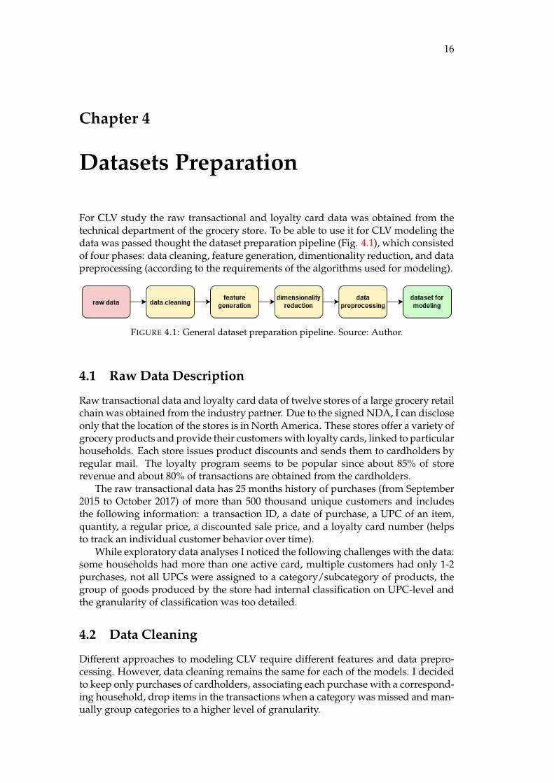
For CLV study the raw transactional and loyalty card data was obtained from thetechnical department of the grocery store. To be able to use it for CLV modeling thedata was passed thought the dataset preparation pipeline (Fig. 4.1), which consistedof four phases: data cleaning, feature generation, dimentionality reduction, and datapreprocessing (according to the requirements of the algorithms used for modeling).

FIGURE 4.1: General dataset preparation pipeline. Source: Author.

4.1 Raw Data Description

Raw transactional data and loyalty card data of twelve stores of a large grocery retailchain was obtained from the industry partner. Due to the signed NDA, I can discloseonly that the location of the stores is in North America. These stores offer a variety ofgrocery products and provide their customers with loyalty cards, linked to particularhouseholds. Each store issues product discounts and sends them to cardholders byregular mail. The loyalty program seems to be popular since about 85% of storerevenue and about 80% of transactions are obtained from the cardholders.

The raw transactional data has 25 months history of purchases (from September2015 to October 2017) of more than 500 thousand unique customers and includesthe following information: a transaction ID, a date of purchase, a UPC of an item,quantity, a regular price, a discounted sale price, and a loyalty card number (helpsto track an individual customer behavior over time).

While exploratory data analyses I noticed the following challenges with the data:some households had more than one active card, multiple customers had only 1-2purchases, not all UPCs were assigned to a category/subcategory of products, thegroup of goods produced by the store had internal classification on UPC-level andthe granularity of classification was too detailed.

4.2 Data Cleaning

Different approaches to modeling CLV require different features and data prepro-cessing. However, data cleaning remains the same for each of the models. I decidedto keep only purchases of cardholders, associating each purchase with a correspond-ing household, drop items in the transactions when a category was missed and man-ually group categories to a higher level of granularity.

Chapter 4. Datasets Preparation 17

4.3 Feature generation

According to selected for the study models, there were three different datasets pre-pared based on transactional and loyalty card data: for clustering (the results ofwhich were later used in Markov Chain, Survival Analytics and Time Series) on 4-weeks aggregated level, for Survival Analytics with aggregation on lifetime durationlevel and Time Series on daily and weekly aggregation level (time series of monthlydata was excluded from the research due to the size of the time period available).

4.3.1 Clustering

The choice of features for clustering was motivated by the idea that the attentionshould be paid not only to the revenue from an individual customer or a cohort butalso to the potentially interesting for customers category of products.•RFM: recency - how recently the household purchase, referring to the number of

days which had passed since the last time a household purchased some goods fromthe store; f requency - how often the household purchase, referring to the number ofinvoices with purchases during the particular month; monetaryvalue - is the amountof money the household spends during a particular month.• Churn: all the history of household’ purchases was considered. If the last pur-

chase was done in the previous to the considered month of purchase and it was notthe last historically available month, then this household was ’churned’.•Discounts: number and monetary value of store coupons, manufacturer coupons,

refunds a household applied during the month.• Categories of Products Purchased - the proportion of money a household spent

on each category of products.• Loyalty program features: duration since a household registered the first loy-

alty card; the number of loyalty cards used by a household.

4.3.2 Survival Analytics

Kaplan-Meier Survival Curves• Churn: same logic as applied above.• Duration: the period in days between the first and the last transactions.

Cox’s Proportional Hazard Model• Churn: same logic as applied above.• Duration: the period in days between the first and the last transactions.• Monetary Value: the amount of money the household spends during a rela-

tionship with a store.• Frequency: the same logic as above.•Mean receipt.• Standard Deviation of a receipt.• Days since the loyalty card was issued.

4.3.3 Time Series

ARIMA/SARIMA/LSTM• ID: household ID or cluster ID.• Date: day or beginning of the week.• Monetary Value: the amount of money a household or a cluster spent in the

store during a particular period – day or week.


4.4 Data Preprocessing

Some clustering algorithms (K-Means, GMM) have requirements for the input data:the variables should be from a symmetric distribution (not skewed) and have thesame average values and variance.

To check the skewness of the data, the distribution of each feature was built.The features with the left skewness were transformed into the logarithmic scale toreshape the distribution into more or less symmetric.

To make the data have the same average values and variance, all features weretransformed using a standard scaler:

z =x− µ

σ(4.1)

where x - value of a variable, µ – mean, σ – standard deviation. Otherwise, inputvariables with larger variances would affect the results of clustering.

4.5 Dimensionality Reduction

In order to avoid misusage of algorithms and biases I checked if the data neededdimensionality reduction, the matrix of correlation was built (Fig. 4.2). However, nostrongly correlated features (with a correlation coefficient > 0.9) were detected thatcould possibly affect the clustering results. Moreover, since the dataset containedonly 21 features, no dimensionality reduction technique was applied.

FIGURE 4.2: Feature Matrix Correlation. Source: Author.

4.6 Summary

The full data engineering cycle of the datasets preparation is considered in thischapter – from the raw data obtained from the company’s technical department to


datasets used in different approaches of modelling CLV. Each step of the data prepa-ration pipeline is provided with a detailed explanation. Moreover, the descriptionof each feature logic in the datasets is provided.

20

Chapter 5

Experiments

5.1 Analytical Environment

The data analysis was executed in the PySpark environment on Google Colab, ex-ploiting their free available GPU (K80 in most cases). I had to contribute some timeand effort on rewriting all the scripts in PySpark syntax, but it helped me not onlywith speeding up the processes (mostly feature generation, feature selection, datapreprocessing before clusterization), but also be on the same page with a scientificsupervisor. Markov Chain, survival analysis and time series forecasting were donein Python. Markov Chain module was written by me, Time Series ARIMA forecast-ing was modeled by statsmodels package (Seabold, Skipper, and Perktold, 2010) andSurvival Analysis was conducted with the help of the lifelines package.

Additionally, there was an attempt to launch NVIDIA’s Rapid in Google Colab;however, I was unlucky to receive access to T4 GPU permanently.

5.2 Clusterization

The preliminary idea of the clustering application in the research is that I have de-tected different behavioural patterns and group all the customers into clusters basedon their historical purchases (taken into account not only revenue and store loyaltybut customers’ basket preferences), investigate purchase activity of each cluster andpredict its value for the store in the future (CLV). The exact data preparation forclusterization techniques is described in Section 4.3.1.

5.2.1 K-Means

To conduct customer clusterization by applying the K-Means algorithm, the numberof centroids should be parametrized. To solve this puzzle, I applied K-Means cluster-ing technique for range of possible number of clusters between 0 and 50, measuringWithin Cluster Sum of Squares (WCSS) (Fig. 5.1), and a Silhouette Score (Fig. 5.2) aswell.

Elbow Method

The algorithm scans through the estimated range of clusters and calculates the sumof squared distances within clusters (WCSS) - how far a point from a cluster it isassigned to. Then the dependence of WCSS on the number of clusters is plotted, anda value (appropriate cluster number) where the curve flattens out is indicated.

Chapter 5. Experiments 21

FIGURE 5.1: Dependence of Within Cluster Sum of Squares (or K-Means score) on the number of clusters (Elbow Method).

Source: Author.

Silhouette Score

According to Sklearn silhouette score documentation, silhouette score (SS) is calculatedusing the mean intra-cluster distance (a) and the mean nearest-cluster distance (b)for each sample and evaluates how close each data point is to its cluster versus howclose it is to the other clusters.

SS =b− a

max(a, b)(5.1)

FIGURE 5.2: Dependence of silhouette score on the number of clusters(K-Means). Source: Author.

From Fig. 5.1 and Fig. 5.2 the exact number of clusters is not obvious. However,it is possible to assume that it is near 20. The silhouette score value is not high,meaning that the clusters are not separable entirely (the best value is 1, the worst is-1, values near 0 indicate overlapping clusters - Sklearn silhouette score documentation).I chose the most promising variants and build the distribution of customers withinclusters (17, 20, 21 clusters) (Fig. 5.3).

K-Means performs extremely fast compared to all other algorithms used in theresearch. A customer distribution within the clusters is relatively good. These threenumbers of clusters are added to further Markov chain modeling.


(A) (B)

(C)

FIGURE 5.3: Histograms of customer distribution within 17(A), 20(B),and 21 (C) clusters (K-Means). Source: Author.

5.2.2 Gaussian Mixture Model

FIGURE 5.4: Dependence of silhouette score on the number of clusters(GMM). Source: Author.

According to the GMM silhouette score metric (Fig. 5.4), the most appropriatenumber of clusters are 8, 11 and 21. However, 17 and 20 also have a high valuecompared to their neighbors.

The chosen number of GMM clusters (Fig. 5.5) showed a less balanced customerdistribution compared to K-Means results. For further investigation, the same num-ber of clusters as for K-Means (17, 20 and 21) was selected.


(A) (B)

(C) (D)

(E)

FIGURE 5.5: Histograms of customer distribution within 8 (A), 11 (B),17 (C), 20 (D), 21 (E) clusters (GMM). Source: Author.

5.2.3 DBSCAN

The application of DBSCAN clustering was not so successful as K-Means or GMM.Although a number of clusters are not required, there are still two parameters tospecify: a distance which indicates how close data points should be to each other tobe considered as a part of a cluster (ε) and a minimum number of data points to beconsidered as a cluster (minPts).

According to Sander et al., 1998 a number of minPts should be set up as largeas a double number of dimensions (dim) in the dataset minPts = 2 dim, and if thedimensionality is high, this number can be increased to get better results. The valueof ε should be chosen as small as possible. One of the methods is to use a k-distancegraph, plotting the distance to the k = minPts − 1 nearest neighbor ordered fromthe largest to the lowest value. Appropriate values of are considered where the plot


shows an "elbow". If ε is too low, a large part of the data will be out of clusters;whereas if ε is high, clusters will merge and the majority of objects will be in thesame cluster.

FIGURE 5.6: The Elbow method to find ε value for DBSCAN.Source: Author.

FIGURE 5.7: Histograms of customer distribution within 8 clusters(DBSCAN). Source: Author.

Since the dataset for clustering has 21 dimensions, minPts is considered to beequal to 42. From Fig. 5.6 it can be found that ε = 2. The results of applyingDBSCAN algorithm are represented in Fig. 5.7. It detects 8 clusters (7 actual and 1assigned for outliers) and shows that more than 20 thousand of households (about75%) are assigned to one cluster and about 3.5 thousand households (about 13%) areconsidered as outliers.

Since the clustering with DBSCAN provides with small number of clusters andshows unbalanced household distribution among clusters (too many outliers andone strongly dominating cluster), it seems that this clustering technique is not appro-priate for our dataset (DBSCAN tends to merge clusters with overlapping regions,and we know from GMM and K-Means that clusters are not entirely separated –have a low silhouette score) I have not included its results into further CLV model-ing.


5.2.4 Summary

In this section, I ran multiple experiments with clustering algorithms (K-Means,GMM, and DBSCAN), figuring out the best one to fit the data. I refused to useDBSCAN results due to its poor performance on the data. I used a silhouette scorefor GMM and both Elbow Method (WCSS metric) and silhouette score for K-Meansclustering to determine the optimal number of clusters. Moreover, I checked the dis-tribution of customers in each clustering result. I decided to use the top three bestresults from K-Means and GMM clustering in further CLV modeling with MarkovChain.

5.3 Markov Chain

5.3.1 CLV modeling

At the beginning of this stage, I had the results from K-Means and GMM clustering(17, 20 and 21 clusters) – overall six different labels for each household in train andtest datasets (5 thousand unique households are taken into account). Using a traindataset (first 20 4-week months) I calculated the transition matrix – a probability tomove from one cluster to another (Fig. 5.8), average revenue and

r = (1− churn rate) (5.2)

for each cluster.To model CLV for the selected period of the time (test number of months: eight

4-week months) I needed first to estimate revenue of each cluster (Fig. 5.9) using thefollowing formula:

Rjn = Tn < Rj > (5.3)

where T – transition matrix, n – number of periods (months of interest), < Rj >–average revenue of a cluster j obtained for the past period (train dataset).

In the example with 21 clusters obtained by K-Means algorithm (Fig. 5.8-5.9) allcustomers who formed the 1st cluster are churners. Thus, the retention rate of the1st cluster equals 0, and for all the rest clusters 1.

Then, CLV per cluster can be estimated as a sum of estimated revenues from nowto a month of interest multiplied by the average retention rate value:

CLVjn =n

∑i=1

Rji < rj > (5.4)

where Rij - estimated revenue for a cluster j in a month i, n – number of peri-ods, < rj >– average retention rate of a cluster j obtained for the past period (traindataset).

5.3.2 Model evaluation

To evaluate a model, a comparison with a ground truth should be performed. Asground truth, I used a test dataset where each household had six predicted labels(17, 20, 21 clusters’ labels from K-Means and GMM) and calculated revenue percluster for eight 4-weeks months (Fig. 5.10).

From Table 5.1 the best result (the lowest error) observed is for 21 clusters ob-tained by running K-Means algorithm. This result proves that the more balanced


FIGURE 5.8: A sample of a Transition Matrix: probability to switchthe cluster in the next month (21-clusters, K-Means). Source: Author.

FIGURE 5.9: A sample of revenue estimation for the next 8 months(21-clusters, K-Means). Source: Author.

clusters the better result could be expected in further modeling. Thus, for survivalanalytics and time series forecasting, I used labels corresponding 21-cluster K-Meansclustering result.

TABLE 5.1: Comparison of Markov Chain RMSE of CLV for differentclustering techniques.

Method of clustering Number of clusters RMSE

K-Means17 714020 498721 4803

GMM17 739620 601721 6596


FIGURE 5.10: A sample of actual Revenue (ground truth for 21-clusters, K-Means). Source: Author.

FIGURE 5.11: A sample of Sankey diagram of customer transitionsbetween clusters. Source: Author.

5.3.3 Business Value vs CLV forecast

A stability of each cluster can be checked in Fig. 5.8. The diagonal elements of thematrix correspond to the probability to stay at the same cluster. Thus, clusters 0, 5, 9,11, 17 and 18 show the highest percent of customers who perform the same purchasebehavior from month to month. Moreover, it is easy to notice that the 1st cluster isformed by churners (customers who left the store this month). From the additionaldata exploration results, no other clusters contain churners. Thus, if a discount rateis neglected, the revenue of a cluster equals its CLV for a particular month.

Customer transitions between their states (belonging to a particular cluster in a


particular time period) can be represented as a Sankey diagram (Fig. 5.11). Sucha representation is particularly valuable from the business perspective, since it dis-plays the customer behavior in more understandable way compared to a transitionmatrix representation. Using this visualization, it is easy to distinguish the customerproportions between clusters and the way it was formed.

FIGURE 5.12: Average predicted CLV vs Current Revenue.Source: Author.

Besides that, if to check predicted average CLV versus current revenue (Fig. 5.12)it is possible to see what actions towards customers could be performed. At the placewhere the considered ratio reaches maximum value the growth is expected, so somepromotions for customers can be applied. At the place where the considered ratiodecreases some recommendations towards a retention actions can be given. Thus,from Fig. 5.12 the most pessimistic scenarios are belonged to the 2nd, 5th and 18thclusters and the most optimistic ones to the 19th, 7th, 10th and 13th clusters.

5.3.4 Summary

In this section, the process of CLV estimation using Markov Chain model was con-sidered. Six experiments were conducted for customer distributions between clus-ters obtained by K-Means and GMM clustering algorithms. The best RMSE wasobtained for 21-cluster customer split by K-Means (the one which showed the mostbalanced customer distribution between clusters (Fig. 5.3)). Moreover, two visual-izations of transitions between clusters and their practical application were consid-ered too.

5.4 Survival Analytics

5.4.1 Cox’s Proportional Hazard Model

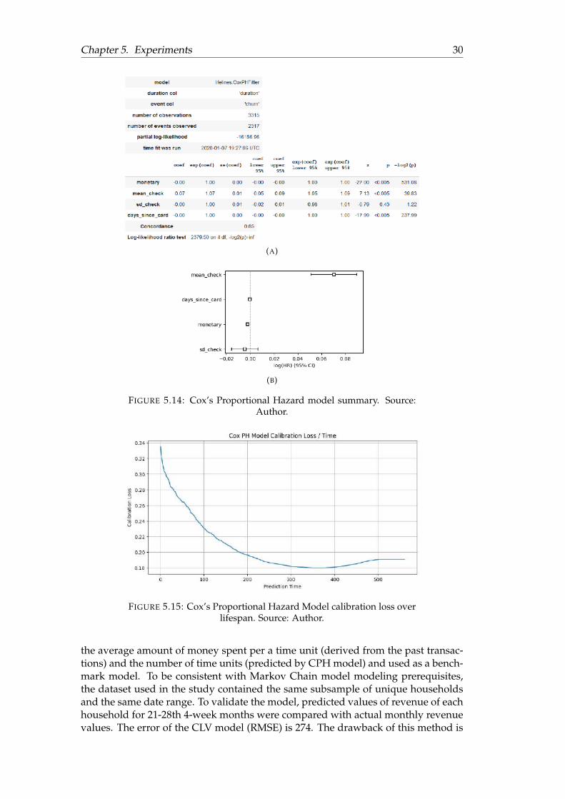
To conduct survival analytics the train and test datasets were generated separately.The dataset included the first 20 4-week months of subsample data with five thou-sand unique households. The data was split with 80% for the train and 20% for thetest. Cox’s Proportional Hazard model summary is represented in Fig. 5.14. As wecan notice (Fig. 5.13), there are those households who are ready to churn alreadyand those who are going to stay with a store in a long relationship.


FIGURE 5.13: The time dependence of the probability to survive.Source: Author.

To obtain the lifespan which can be used together with time series revenue pre-dictions, the CPH model (Fig. 5.14) was used to predict the behavior of the cus-tomers starting from the 21st 4-week month. The predicted lifespan was corre-sponded to the whole period of relationships without linkage to the calendar dates,to know how many days left for a particular household it is needed to subtract thenumber of days from the first purchase to the date the modeling was conducted. Athreshold of survival probability was set as 0.5 (however, it can be set to a highervalue to be more precise) to obtain the lifespan of the relationship between a storeand a particular household.

5.4.2 Accuracy and calibration of CPH model

The concordance index (a fraction of all pairs of subjects whose predicted survivaltimes are correctly ordered among all subjects that can actually be ordered, Raykar)of the CPH model is 85%.

From the calibration curve above (Fig. 5.15) it can seen that the model has thebest performance when predicting lifespan is located between 300 and 400 days.As examples, let’s check the calibration plots for lifespan at 100 and 450 days (Fig.5.16) – examining various probabilities against fractions that are present in the testdataset. The diagonal line represents perfect calibration. The model underpredictsthe risk to churn for lifespans equals 100. For lifespan equals 450, the model slightlyunderpredicts risk to churn at the probability of less than 20% and overpredict riskto churn at the probability of more than 20%.

From Fig. 5.15 and Fig. 5.16 it can be deriven that the longer the customer stayswith a company, the better churn prediction is. However, it is worth mentioningthat the train dataset contained 80 weeks (560 days) date range only, so the max-imum possible value of the lifespan was 560. If to check the predicted values oflifespan, it can be noticed that 65% of them were predicted as infinity (means thatthese customers are loyal and not going to churn from the store) and replaced withlifespan equals 600 for visualization (Fig. 5.17).

5.4.3 CPH CLV Benchmark model

Preliminary I was going to use the result of CPH modeling together with Time Seriespredictions only. However, CLV can also be roughly estimated as a multiplication of


(A)

(B)

FIGURE 5.14: Cox’s Proportional Hazard model summary. Source:Author.

FIGURE 5.15: Cox’s Proportional Hazard Model calibration loss overlifespan. Source: Author.

the average amount of money spent per a time unit (derived from the past transac-tions) and the number of time units (predicted by CPH model) and used as a bench-mark model. To be consistent with Markov Chain model modeling prerequisites,the dataset used in the study contained the same subsample of unique householdsand the same date range. To validate the model, predicted values of revenue of eachhousehold for 21-28th 4-week months were compared with actual monthly revenuevalues. The error of the CLV model (RMSE) is 274. The drawback of this method is


(A) (B)

FIGURE 5.16: Example of Calibration plots for the lifespan of 100 (A)and 450 (B) days. Source: Author.

(A) (B)

FIGURE 5.17: Customer distribution by lifespan: actual versus pre-dicted. Source: Author.

that future customers are eliminated from the CLV modeling.

5.4.4 Summary

In this section, Cox’ Proportional Hazard Model was explored. By running themodel, the lifespan for the customers was predicted. However, to be able to use itin further calculations, a threshold for the probability to survive was required to beset, and the number of days since customer’s first transaction should be subtractedfrom the predicted values of lifespans. Then the model performance was checked byexploring calibration curve. In addition, Cox’ Proportional Hazard CLV Benchmarkmodel was built.

5.5 Time Series Forecasting

For the time series forecasting, I used data with labels for 21 clusters obtained by theK-Means algorithm. There are multiple approaches on how to aggregate the data toproceed with the revenue forecast: aggregation on household and cluster level on adaily, weekly and monthly (4-week month) basis.

A monthly aggregation approach for both individual and cluster level was ex-cluded from the study at the very beginning due to too narrow date range in the


available dataset (assuming that 20 points are not enough to build a good time se-ries prediction model according to Groebner et al., 2010 a sufficiently large sampleis equal at least 30).

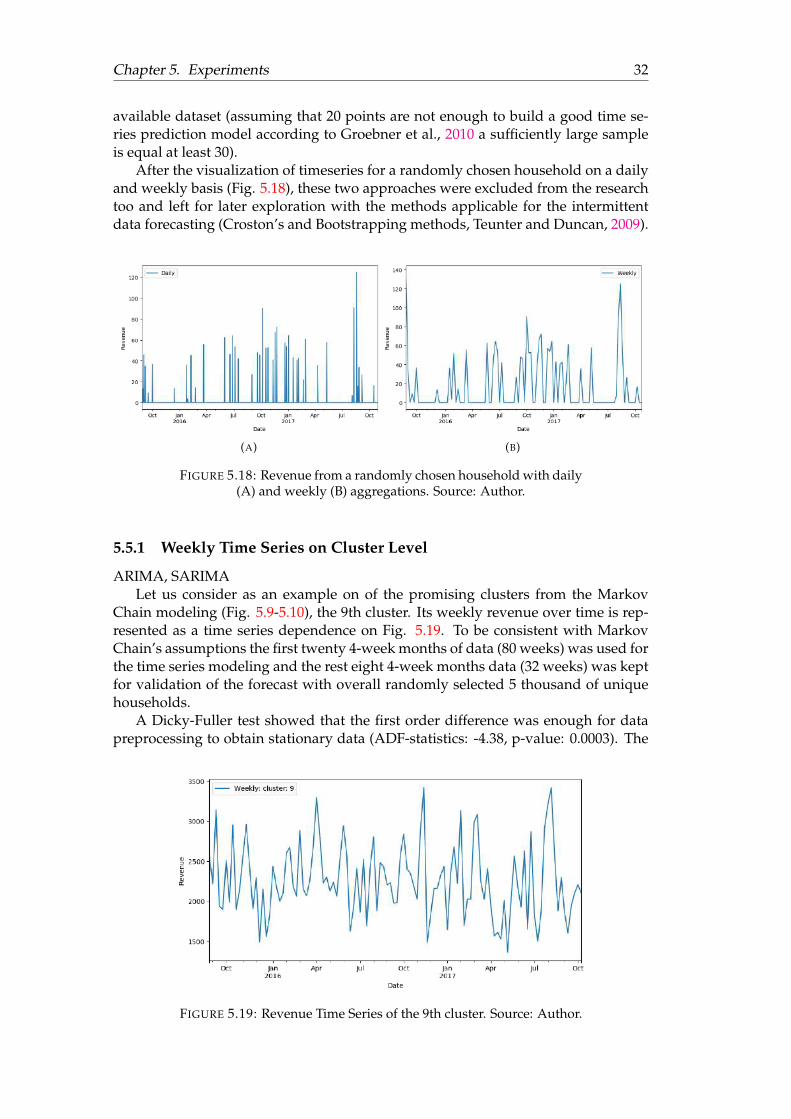
After the visualization of timeseries for a randomly chosen household on a dailyand weekly basis (Fig. 5.18), these two approaches were excluded from the researchtoo and left for later exploration with the methods applicable for the intermittentdata forecasting (Croston’s and Bootstrapping methods, Teunter and Duncan, 2009).

(A) (B)

FIGURE 5.18: Revenue from a randomly chosen household with daily(A) and weekly (B) aggregations. Source: Author.

5.5.1 Weekly Time Series on Cluster Level

ARIMA, SARIMALet us consider as an example on of the promising clusters from the Markov

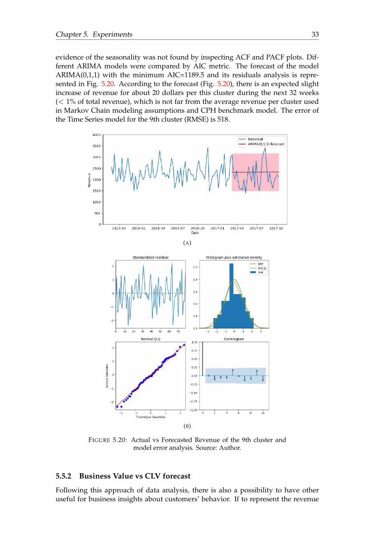
Chain modeling (Fig. 5.9-5.10), the 9th cluster. Its weekly revenue over time is rep-resented as a time series dependence on Fig. 5.19. To be consistent with MarkovChain’s assumptions the first twenty 4-week months of data (80 weeks) was used forthe time series modeling and the rest eight 4-week months data (32 weeks) was keptfor validation of the forecast with overall randomly selected 5 thousand of uniquehouseholds.

A Dicky-Fuller test showed that the first order difference was enough for datapreprocessing to obtain stationary data (ADF-statistics: -4.38, p-value: 0.0003). The

FIGURE 5.19: Revenue Time Series of the 9th cluster. Source: Author.


evidence of the seasonality was not found by inspecting ACF and PACF plots. Dif-ferent ARIMA models were compared by AIC metric. The forecast of the modelARIMA(0,1,1) with the minimum AIC=1189.5 and its residuals analysis is repre-sented in Fig. 5.20. According to the forecast (Fig. 5.20), there is an expected slightincrease of revenue for about 20 dollars per this cluster during the next 32 weeks(< 1% of total revenue), which is not far from the average revenue per cluster usedin Markov Chain modeling assumptions and CPH benchmark model. The error ofthe Time Series model for the 9th cluster (RMSE) is 518.

(A)

(B)

FIGURE 5.20: Actual vs Forecasted Revenue of the 9th cluster andmodel error analysis. Source: Author.

5.5.2 Business Value vs CLV forecast

Following this approach of data analysis, there is also a possibility to have otheruseful for business insights about customers’ behavior. If to represent the revenue


as an average per cluster with its forecast (Fig. 5.21) and plot CPH model curves foreach household who form the cluster (Fig. 5.22), the average expected revenue froma single household and its stability over time in terms of lifespan can be checked.As for the 9th cluster, the average value of revenue per household fluctuates around30 dollars and customers of the cluster are expected to stay with a company with aprobability of 50% for at least 250 days.

FIGURE 5.21: Average revenue per customer of the 9th cluster.Source: Author.

FIGURE 5.22: Probability to survive for the households of the 9thcluster: general and at the point of lifespan prediction. Source: Au-

thor.

A similar conclusion can be derived from the Markov Chain probability matrix(Fig. 5.8). The 9th cluster performs relatively stable towards churners of the store aswell as switchers to the other clusters.

5.5.3 Summary

In this section, a time series approach for revenue estimates was checked on individ-ual and cluster level. As an example of the model results the 9th cluster. The outputof the model together with the results of Cox’ Proportional Hazard model (lifespan)was used in CLV calculations. Moreover, it was shown how to use both methodsto extract other valuable information for the business. To be able to compare the


performance of the model with Markov Chain model output, the estimation of CLVwas done on weekly aggregated data and then mapped to months.

5.6 Summary

In this research, three different clusterization techniques (K-Means, GMM, DBSCAN)were examined towards a performance on the transactional and loyalty card datawith a chosen feature set. K-Means has shown the best result in terms of speed andthe quality of customer distribution in clusters. The output of the clustering ap-proaches was later used in Markov Chain, Survival Analytics, and Time Series CLVmodeling.

The fundamental part of the Markov Chain model used for CLV modeling wasa state definition. The states represented by customer clusters had three main com-ponents: a retention rate, a revenue and a behavioral pattern (probability to movebetween clusters). Markov Chain CLV estimates were modeled based on transi-tion probabilities (derived from the historical transactional data), average clustermonthly revenues realized within the first 20 4-week months and an average reten-tion rate per cluster

On the other hand, econometric Cox’ Proportional Hazard model estimated acustomer probability to churn in a particular period taken into account the factorswhich could cause such an event. Time Series Forecasting techniques estimated thevalue of revenue for future periods which was approximately equal to an averagerevenue per cluster obtained in the past. The results of both models were combinedin CLV estimates.

Finally, when a particular cluster was considered within results of both mod-els, the general picture obtained by a probabilistic approach on a cluster level wasproven by econometric approach on an individual one.

36

Chapter 6

Conclusions and Future Work

6.1 Conclusions

CLV is an important metric for retail since it indicates the success of the marketingcampaigns and channels, deals with retention and churn, and helps with decisionstowards resource allocation. However, the modeling of CLV for retail is a challeng-ing task due to the lack of access to the historical data of purchases and difficulty ofcustomer identification.

In this research, an analytical framework for offline and semi-offline businesseswas prototyped (Kasprova, 2020: CLV for Retail) to estimate CLV based on transac-tional and loyalty card data . This framework transfers the raw data obtained fromthe grocery store operational databases to business insights based on CLV estimatesand their visualizations. It can be used for channels and campaign evaluations.

According to the data pipeline of the framework, the transactional data of thestore linked to the loyalty card data provides historical references of purchases tocorresponding customers. Then customers are segmented based on the similarityof their purchase behavior performed by clusterization algorithms. Markov Chainprobabilistic model applied to segments of customers shows a general picture of theongoing processes which are easy to interpret exploring the Sankey diagram. Tohave more details on an individual level to transfer the previously received infor-mation into data-driven decisions or possible actions towards CRM and resourcesallocation Time Series revenue forecasts, together with Cox’s Proportional Hazardmodel, lifetime estimates are used.

There are a few limitations of the research that should be highlighted. The pro-posed approaches of CLV estimations were developed for existing customers only.The framework was developed using 1.5-year data and tested only on 0.5-year data.It can be significantly improved using a dataset with the broader data range, at leastto be able to make monthly based aggregations for the Time Series predictions. Theaim of the research and a framework development had a more conceptual charac-ter rather than accuracy-oriented. Thus, there is a variety of methods, which can beexplored for a more efficient revenue and churn prediction in the future.

6.2 Future Work

1. To check other time series analysis approaches: classical - Facebook Prophet,VARMAX, Holz-Winter, and RNN – LSTM, seq2seq, ES-RNN, DeepAR etc.

2. To explore ARIMAX/SARIMAX models to be able to check the performanceof multivariate time series and compare the obtained results with my current stateof art model, including public holidays, school vacation, store location, and festivalsnearby, shop holidays, fasting and abstinence as exogenous variables.

Chapter 6. Conclusions and Future Work 37

3. To explore time series approaches to predict revenue on customer level whenthe data is intermittent: Croston’s and Bootstrapping methods (Teunter and Duncan,2009).

4. To predict churn using machine learning approaches such as logistic regres-sion, binary classification with XGBoost, SVM, Random Forest, etc.

5. To segment customers based on their revenue and then include their tastefeatures.

6. To extend modeling to other stores.7. To develop interactive visualization of results in Dash (a visualization frame-

work with a Python backend).

38

Bibliography

Batislam E.and Denizel, M. and A Filiztekin (2007). “Empirical Validation and Com-parison of Models for Customer Base Analysis”. In: International Journal of Re-search in Marketing 24.3, pp. 201–209.

Bishop, Ch. (2006). Pattern Recognition and Machine Learning. Springer-Verlag NewYork.

Brownlee, J. (2018). Introduction to Time Series Forecasting with Python. v.1.4, e-book.Cox, D. (1972). “Regression Models and Life Table”. In: Journal of the Royal Statistical

Society, Series B 34.2, pp. 187–220.Damodaran, A. (2020). Cost of Capital by Sector (US). URL: http://people.stern.

nyu.edu/adamodar/New_Home_Page/datafile/wacc.html. Accessed: 2020-01-08.Ester, M. et al. (1996). “A Density-Based Algorithm for Discovering Clusters in Large

Spatial Databases with Noise”. In: Proceedings of the 2nd International Conferenceon Knowledge Discovery and Data Mining, AAAI Press, Portland, pp. 226–231.

Estrella-Ramón, A. et al. (2013). “A marketing view of the customer value: Customerlifetime value and customer equity”. In: South African Journal of Business Manage-ment 44.4, 47–64.

Forecasting using ARIMA models in Python. URL: https : / / www . datacamp . com /courses/forecasting- using- arima- models- in- python. Accessed: 2020-01-08.

Fox, E. and C. Guestrin (2016). Gaussian Mixture Model for Clustering. https://www.youtube.com/watch?v=DODphRRL79c. Accessed: 2020-01-08.

Groebner, D. et al. (2010). Business Statistic. 8th edn, Pearson.Gupta, S. et al. (2006). “Modeling Customer Lifetime Value”. In: Journal of Service

Research 9, pp. 139–155.Haenlein, M., A. Kaplan, and A. Beeser (2007). “A Model to Determine Customer

Lifetime Value in a Retail Banking Context”. In: European Management Journal25.3, 221–234.

Hughes, A. (2011). Strategic Database Marketing. 4th edn.,McGraw-Hill, New York.Jasek, P. et al. (2018). “Modeling and Application of Customer Lifetime Value in On-

line Retail”. In: Informatics.Jasek, P. et al. (2019). “Predictive performance of customer lifetime value models in

e-commerce and the use of non-financial data”. In: Prague Economic Papers.K-Means and X-Means Clustering. https://www.brandidea.com/kmeans.html. Ac-

cessed: 2020-01-08.Kaplan, L. and P. Meier (1958). “Nonparametric Estimation form Incomplete Obser-

vations”. In: Journal of American Statistical Association 53.6, 457–481.Kasprova, A. CLV for Retail. https://github.com/kasprova/advanced_customer_

analytics. Accessed: 2020-01-08.Kotler, P. (1974). “Marketing During Periods of Shortage”. In: Journal of Marketing

38.3, 20–29.Lloyd, S. (1982). “Least square quantization in PCM”. In: IEEE Transactions on Infor-

mation Theory 28.2, pp. 129–137.

http://people.stern.nyu.edu/adamodar/New_Home_Page/datafile/wacc.html

http://people.stern.nyu.edu/adamodar/New_Home_Page/datafile/wacc.html

https://www.datacamp.com/courses/forecasting-using-arima-models-in-python

https://www.datacamp.com/courses/forecasting-using-arima-models-in-python

https://www.youtube.com/watch?v=DODphRRL79c

https://www.youtube.com/watch?v=DODphRRL79c

https://www.brandidea.com/kmeans.html

https://github.com/kasprova/advanced_customer_analytics

https://github.com/kasprova/advanced_customer_analytics

Bibliography 39

Machine Learning for Marketing Analytics in R. https : / / campus . datacamp . com /courses/marketing-analytics-in-r-statistical-modeling. Accessed: 2020-01-08.

McKinsey. Customer Lifecycle Management. https://www.mckinsey.com/business-functions/marketing-and-sales/how-we-help-clients/customer-lifecycle-management. Accessed: 2020-01-08.

Miller, R. (2011). Survival analysis. 2nd edn., Wiley.Mittal, A. (2019). Understanding RNN and LSTM. URL: https://towardsdatascience.

com/understanding-rnn-and-lstm-f7cdf6dfc14e. Accessed: 2020-01-08.Neslin, S. et al. (2006). “Defection detection: Measuring and understanding the pre-

dictive accuracy of customer churn models”. In: Journal of Marketing Research 46.5,pp. 204–211.

Nikkhahan, B., Badrabadi A. Habibi, and M Tarokh (2011). “Customer Lifetime Valuemodel in an online toy store”. In: Journal of Industrial Engineering International7.12, pp. 19–31.

Overview of clustering methods. https : / / scikit - learn . org / stable / modules /clustering.html. Accessed: 2020-01-08.

Pfeifer, P. and R. Carraway (2000). “Modelling customer relationships as Markovchains”. In: Journal of Interactive Marketing 14.2, pp. 43–55.

Sander, J. et al. (1998). “Density-based clustering in spatial databases: The algorithmGDBSCAN and its applications”. In: Data Mining and Knowledge Discovery 2 2,169–194.

Schubert, E. et al. (2017). “DBSCAN revisited, revisited: why and how you should(still) use DBSCAN”. In: ACM Transactions on Database Systems (TODS) 42.3, p. 19.

Seabold, Skipper, and Josef. Perktold (2010). “Statsmodels: Econometric and statisti-cal modeling with python”. In: Proceedings of the 9th Python in Science Conference.

Sklearn silhouette score documentation. https://scikit-learn.org/stable/modules/generated/sklearn.metrics.silhouette_score.html. Accessed: 2020-01-08.

Teunter, R. and L. Duncan (2009). “Forecasting intermittent demand: a comparativestudy”. In: Journal of the Operational Research Society 60.3, pp. 321–329.

Villanueva, J. and D. Hanssens (2007). “Customer equity: Measurement, manage-ment and research opportunities”. In: Foundations and Trends in Marketing 1.1,pp. 1–95.

Wedel, M. and W. Kamakura (1999). Market Segmentation: Conceptual and Methodolog-ical Foundations. 2nd edn. Kluwer Academic Publishers, Boston.

https://campus.datacamp.com/courses/marketing-analytics-in-r-statistical-modeling

https://campus.datacamp.com/courses/marketing-analytics-in-r-statistical-modeling

https://www.mckinsey.com/business-functions/marketing-and-sales/how-we-help-clients/customer-lifecycle-management



https://towardsdatascience.com/understanding-rnn-and-lstm-f7cdf6dfc14e

https://towardsdatascience.com/understanding-rnn-and-lstm-f7cdf6dfc14e

https://scikit-learn.org/stable/modules/clustering.html

https://scikit-learn.org/stable/modules/clustering.html

https://scikit-learn.org/stable/modules/generated/sklearn.metrics.silhouette_score.html

https://scikit-learn.org/stable/modules/generated/sklearn.metrics.silhouette_score.html

Customer Lifetime Value for Retail Based on Transactional ...

Documents

Transcript of Customer Lifetime Value for Retail Based on Transactional ...