
Implementing Usability Testing Of Technical Documents At ...
Upload
khangminh22Category
view
1download
0
Thesis for the Degree of Doctor of TechnologySundsvall 2013
On the Lifetime and Usability ofEnvironmental Monitoring Wireless
Sensor Networks
Sebastian Bader
Supervisor: Professor Bengt Oelmann
Department of Electronics DesignMid Sweden University, SE-851 70 Sundsvall, Sweden
ISSN 1652-893XMid Sweden University Doctoral Thesis 161
ISBN 978-91-87557-04-0

Akademisk avhandling som med tillstand av Mittuniversitetet i Sundsvallframlaggs till offentlig for avlaggande av doctorexamen i elektronik onsdagden 2 oktober 2013, klockan 13:30 i sal L111, Mittuniversitetet Sundsvall.Seminariet kommer att hallas pa engelska.
On the Lifetime and Usability of Environmental Monitor-ing Wireless Sensor Networks
Sebastian Bader
©Sebastian Bader, 2013
Department of Electronics DesignMid Sweden University, SE-851 70 SundsvallSweden
Telephone: +46 (0)60 148495
Printed by Kopieringen Mittuniversitetet, Sundsvall, Sweden, 2013
Abstract
Wireless sensor networks have been demonstrated, at an early stage in theirdevelopment, to be a useful measurement technology for environmentalmonitoring applications. Based on their independence from existing infras-tructures, wireless sensor networks can be deployed in virtually any locationand provide sensor samples in a spatial and temporal resolution, which oth-erwise would only be achievable at high cost or involve significant work byhumans. The feasibility of the usage of wireless sensor networks in real-worldapplications, however, is only maintained if certain technological challengesare overcome. Amongst these challenges, are the limited lifetime of the dis-tributed sensor nodes, and user interfaces, which allow for the technologyto be utilized in an efficient manner. Contributions to the solution of thesechallenges have been the objective of this thesis.
After an analysis of the contributions wireless sensor networks can provideto the application domain of environmentalmonitoring, and the introductionto the restrictions, which are posed by a limited operational lifetime and lowsystem usability, these issues are addressed at the system level of sensor nodedevices.
The lifetime of sensor nodes, which is closely linked to the lifetime of thecomplete wireless sensor network, is addressed with regards to the energyefficiency of nodes, as well as the utilization of solar energy harvesting inorder to increase the available energy resources. With respect to energyefficiency, an analysis has been performed of the contributions to the energyconsumption of environmental monitoring sensor nodes, which leads to thedesire to minimize the nodes’ duty cycles and quiescent currents. A sensornode design is presented, which features energy efficiency as a key attributeby utilizingmodern semiconductor architectures. Moreover, an argument forthe usage of synchronization-based, contention-free communication is madein order to reduce active communication periods and, thus, the duty cycleof a sensor node. A synchronization method with its focus on low protocol
i

Abstract
overhead is introduced as a basis for such communication forms.After an initial feasibility study in relation to using battery-less solar energy
harvesting architectures in locations with limited solar irradiation, multi-ple architectural implementations are analyzed in a comparative manner.Among these comparisons is an analysis of short-term energy storage devicesin the form of double-layer capacitors and thin-film batteries, which provideprolonged component lifetimes than those for conventional secondary bat-teries, but which can only buffer for short periods of time due to their limitedenergy capacity. In order to be able to dimension such energy harvestingsystems with respect to the individual application constraints at hand, state ofcharge simulations are proposed. Amethod for such simulations is presentedand demonstrated for the implementation of an energy harvester model on acomponent basis. While the modeling in this manner is time consuming, themodel can predict the state of charge of the energy buffer in the architecturewith a high level of accuracy. Finally, a method for the systematic evaluationof solar energy harvesting architectures is presented. The presented methodcan be summarized as a solar energy harvesting testbed, which utilizes config-urable energy harvesting circuits in order to create a deploy-once-test-manytype of system. The output results of this testbed can significantly improvethe efficiency of architecture comparisons and system modeling.
Contributions to the improvement of the usability of wireless sensor nodesare made on two separate levels, namely, developer usability and end userusability. A method for the programming of sensor nodes based on hier-archical finite state machines is presented, which improves the usability ofsoftware development by creating familiarity for technically experiencedusers. Moreover, the utilization of finite state machine principles allowsfor the software to be developed in a systematic and modular manner. Asimplemented applications typically require to be verified, which, in the en-vironmental monitoring domain, usually results in outdoor deployments,usability considerations for sensor nodes are presented, which can simplifythis process. Special attention has been paid in order for these improvementsto be achieved with low overheads.While software development is a familiar concept for most system devel-
opers, this is not the case for the end users of these systems, who are typicallydomain experts. In order to allow for wireless sensor nodes to be operatedby domain experts, a method for the configuration of sensor nodes has been
ii

proposed. The method uses a combination of graphical specification of thenode behavior and a configurable sensor node. The evaluation of this method,which has been based on a proof-of-concept implementation, demonstratedthat the performance can remain high, while end users, without technicalexperience, are enabled to configure sensor nodes without prior training.In summary, the contributions, presented in this thesis, address system
lifetime and usability with regards to the sensor node level. The results haveled to the implementation of an energy efficient sensor node, which allows forthe operation from battery-less solar energy harvesting sources. Furthermore,support tools for the implementation of these nodes, both on the hardwareand software level, have been proposed.
iii


Acknowledgements
During the last years, there have been a number of people, who were, bothdirectly and indirectly, involved in the process that has led to the work pre-sented in this thesis. I would like to take the opportunity, at this point, toshow my gratitude.First and foremost, I want to thank my main supervisor, Professor Bengt
Oelmann, who has given me the opportunity to conduct this work and whohas supported me during the years. I am very grateful for your guidance, butalso the freedom and trust, which made my work develop the way it did.
I thank my colleagues at the Electronics Design Department for creating agreat work environment. In particular, I want to thank Peng Cheng, StefanHaller, David Krapohl and Najeem Lawal, who I can always count on to beavailable for interesting discussions. I also thank Johan Siden, who has takenthe time to review this work.
I thankMatthias Kramer, Torsten Scholzel, Matthias Anneken andManuelGoldbeck, who have been involved in individual projects that have con-tributed to the work that is presented in this document. Particular apprecia-tion goes to Matthias Kramer, who has been a great support in the technicalimplementation of a number of systems and who always shared my fascina-tion for the technical development in wireless embedded systems.Furthermore, I am grateful to Michael Brunig and Wen Hu, who have
given me the chance to broaden my horizon and who have been supervisingme duringmy stay at CSIRO. I also like to thank everyone at the AutonomousSystems Laboratory for turning my stay in Australia into a great experience.Finally, I thank my family and friends for bringing balance to my life. I
am very grateful to know that you are there and that I can count on yoursupport.
v


Acronyms
CSMA Carrier Sense Multiple Access
CTS Clear-to-Send
DLC Double Layer Capacitor
DSP Digital Signal Processor
EPR Equivalent Parallel Resistance
FDMA Frequency Division Multiple Access
FPGA Field Programmable Gate Array
FSM Finite State Machine
FTSP Flooding Time Synchronization Protocol
GPRS General Packet Radio Service
GSM Global System for Mobile Communications
GUI Graphical User Interface
HAL Hardware Abstraction Layer
HFSM Hierarchical Finite State Machine
IC Integrated Circuit
IEEE Institute of Electrical and Electronics Engineers
IoT Internet of Things
ISM Industrial, Scientific and Medical
vii

Acronyms
ISR Interrupt Service Routine
MCU Micro Controller Unit
MPP Maximum Power Point
MPPT Maximum Power Point Tracking
NiCd Nickel-Cadmium
NiMH Nickel-Metal Hydride
LDO Low Dropout
LOS Line of Sight
LTS Lightweight Time Synchronization
Li-Ion Lithium-Ion
PBS Pairwise Broadcast Synchronization
PCB Printed Circuit Board
PnO Perturb-and-Observe
RBS Reference Broadcast Synchronization
RF Radio Frequency
RTC Real-Time Clock
RTS Request-to-Send
SFD Start Frame Delimiter
SMPS Switch Mode Power Supply
SOC State-of-Charge
TDMA Time Division Multiple Access
TDP Time Diffusion Protocol
viii

TFB Thin-Film Battery
TPSN Timing-Sync Protocol for Sensor Networks
USB Universal Serial Bus
WLAN Wireless Local Area Network
WSN Wireless Sensor Network
ix


Contents
Abstract i
Acknowledgements v
Acronyms vii
List of Figures xiii
List of Tables xvii
List of Papers xix
1 Introduction 11.1 Environmental Monitoring . . . . . . . . . . . . . . . . . . . . 21.2 Wireless Sensor Networks . . . . . . . . . . . . . . . . . . . . 3
1.2.1 Environmental Monitoring with Wireless SensorNetworks . . . . . . . . . . . . . . . . . . . . . . . . . 6
1.2.2 Application Scenario under Scope . . . . . . . . . . . 81.3 Case Study - SAQnet . . . . . . . . . . . . . . . . . . . . . . . 10
1.3.1 Background, Architecture and Implementation . . . 111.3.2 Project Analysis . . . . . . . . . . . . . . . . . . . . . . 15
1.4 Application Analysis . . . . . . . . . . . . . . . . . . . . . . . . 181.5 Problem Formulation . . . . . . . . . . . . . . . . . . . . . . . 201.6 Thesis Contributions . . . . . . . . . . . . . . . . . . . . . . . 211.7 Thesis Outline . . . . . . . . . . . . . . . . . . . . . . . . . . . 22
2 Energy Efficiency 252.1 Wireless Sensor Network Lifetime . . . . . . . . . . . . . . . . 252.2 Wireless Sensor Node Architecture . . . . . . . . . . . . . . . 26
xi

Contents
2.3 Duty-Cycling . . . . . . . . . . . . . . . . . . . . . . . . . . . . 302.4 Energy-efficient Sensor Node Design . . . . . . . . . . . . . . 35
2.4.1 SENTIO-em Architecture and Implementation . . . 362.4.2 SENTIO-em Evaluation . . . . . . . . . . . . . . . . . 41
2.5 Energy-efficient Communication . . . . . . . . . . . . . . . . 452.5.1 Time Synchronization for Wireless Sensor Networks 472.5.2 Synchronized Duty-Cycling . . . . . . . . . . . . . . . 54
3 Solar Energy Harvesting 673.1 Solar Energy Harvesting . . . . . . . . . . . . . . . . . . . . . 67
3.1.1 Energy Neutral Operation . . . . . . . . . . . . . . . . 693.2 Solar Energy Harvesting Architectures . . . . . . . . . . . . . 71
3.2.1 Low Irradiance Conditions . . . . . . . . . . . . . . . 773.2.2 Short-Term Energy Buffers . . . . . . . . . . . . . . . 83
3.3 Solar Energy Harvesting Dimensioning . . . . . . . . . . . . 903.3.1 Modeling of the Solar Energy Harvesting Architecture 913.3.2 Simulating Available Energy Levels . . . . . . . . . . 95
3.4 Solar Energy Harvesting Testbed . . . . . . . . . . . . . . . . 983.4.1 Architecture and Implementation . . . . . . . . . . . 1013.4.2 Setup and Results . . . . . . . . . . . . . . . . . . . . . 105
4 Usability 1114.1 Usability in Wireless Sensor Networks . . . . . . . . . . . . . 1114.2 Usability for Developers . . . . . . . . . . . . . . . . . . . . . . 112
4.2.1 Programming with Hierarchical Finite State Machines 1134.2.2 Usability Considerations for Sensor Nodes . . . . . . 119
4.3 Usability for End Users . . . . . . . . . . . . . . . . . . . . . . 1234.3.1 Concealing Node Programming Complexity . . . . . 124
5 Discussion and Conclusions 131
Bibliography 139
Papers 149
xii

List of Figures
1.1 Comparison of environmentalmonitoring sampling techniques 41.2 Network architecture of applications under scope . . . . . . . 91.3 SAQnet system architecture . . . . . . . . . . . . . . . . . . . 121.4 SAQnet node architecture . . . . . . . . . . . . . . . . . . . . 121.5 Deployment overview of the SAQnet system . . . . . . . . . . 141.6 Energy profile of a SAQnet node . . . . . . . . . . . . . . . . . 151.7 Packaging of a SAQnet node . . . . . . . . . . . . . . . . . . . 17
2.1 General sensor node architecture . . . . . . . . . . . . . . . . 272.2 Graphical representation of the duty-cycling principle . . . . 312.3 Duty-cycling effect on the overall current consumption . . . 352.4 Architectural structure of the SENTIO-em platform . . . . . 372.5 Temperature influence on the SENTIO-em quiescent currents 432.6 Temperature influence on the SENTIO-em communication
currents . . . . . . . . . . . . . . . . . . . . . . . . . . . . . . . 432.7 Evaluation of the processing performance of SENTIO-em . . 442.8 Energy efficiency comparison of sensor node platforms . . . 452.9 Structure of a typical TDMA protocol . . . . . . . . . . . . . 472.10 Occurrence of delay components during a packet transmission 522.11 Unilateral and bidirectional synchronization methods . . . . 532.12 Interval-measurement based synchronization . . . . . . . . . 562.13 Master-Slave synchronization procedure implementation . . 592.14 Accuracy results of the synchronization method . . . . . . . 602.15 Temperature dependency of wake-up accuracy (oven) . . . . 612.16 Temperature dependency of wake-up accuracy (freezer) . . . 622.17 In-box temperature of a plastic enclosure in direct sunlight . 632.18 Comparison of temperature drift behavior . . . . . . . . . . . 632.19 Power consumption of temperature drift compensation . . . 66
xiii
List of Figures
3.1 Simplified energy supply time from an AA-type battery . . . 683.2 Energy harvesting system overview . . . . . . . . . . . . . . . 713.3 Energy density and power density of energy storage devices . 723.4 Characteristics of a small-scale solar panel . . . . . . . . . . . 743.5 Accuracy of MPPT based on fractional open-circuit voltage
and fractional short-circuit current . . . . . . . . . . . . . . . 763.6 Annual solar irradiance distribution in Sundsvall, Sweden . . 783.7 Directly coupled energy harvesting circuit architecture . . . 793.8 Ideal and real zener-diode characteristics . . . . . . . . . . . . 803.9 System behavior of the solar energy harvesting architecture
during one week of deployment . . . . . . . . . . . . . . . . . 823.10 Architecture of the configurable energy harvesting module . 853.11 Experimental setup for short-term energy storage architec-
ture evaluation . . . . . . . . . . . . . . . . . . . . . . . . . . . 863.12 Comparison of the charge behavior of DLCs and TFBs . . . . 863.13 Peak discharge behavior of double layer capacitors and thin-
film batteries . . . . . . . . . . . . . . . . . . . . . . . . . . . . 873.14 Configurable solar energy harvester results (summer) . . . . 883.15 Configurable solar energy harvester results (winter) . . . . . 883.16 MPPT utilization during periods of low irradiation . . . . . . 903.17 Design constraints of solar energy harvesting systems . . . . 913.18 Systemmodel overview for solar energy harvesting simulations 923.19 Equivalent circuit of a solar cell . . . . . . . . . . . . . . . . . 933.20 Equivalent circuit of a DLC . . . . . . . . . . . . . . . . . . . . 943.21 Overview of the solar energy harvesting system model on
high abstraction level . . . . . . . . . . . . . . . . . . . . . . . 953.22 Solar energy harvesting system model evaluation . . . . . . . 953.23 Exemplar output of solar energy harvesting simulation sweeps 973.24 Conceptual overview of the solar energy harvesting testbed . 1003.25 Layered architecture of the solar energy harvesting testbed . 1013.26 Architecture of the configurable energy harvesting module
for the testbed nodes . . . . . . . . . . . . . . . . . . . . . . . 1023.27 Timeline of the testbed communication protocol . . . . . . . 1043.28 Implementation of the configurable solar energy harvesting
testbed nodes . . . . . . . . . . . . . . . . . . . . . . . . . . . . 105
xiv
List of Figures
3.29 Energy profile of a sensor node with sampling and commu-nication tasks . . . . . . . . . . . . . . . . . . . . . . . . . . . . 106
3.30 Comparison of ideal and measured load emulation for theconfigurable load profiles on testbed nodes . . . . . . . . . . 107
3.31 Energy profile of a testbed node in operation . . . . . . . . . 1083.32 Output results of the solar energy harvesting testbed . . . . . 109
4.1 State-graph representation of a sample-and-send application 1144.2 Layered architecture of the HFSM framework implementation 1164.3 Program flow of the execution of state transitions . . . . . . . 1174.4 Picture of the SENTIO-em platform implementation . . . . . 1214.5 Conventional process of sensor system implementations . . . 1254.6 Adapted sensor system implementation process . . . . . . . . 1254.7 State-graph of the configurable sensor node firmware . . . . 1274.8 Implementation of the configurable sensor node design . . . 128
xv


List of Tables
1.1 Component implementation of SAQnet nodes . . . . . . . . 131.2 Environmental monitoring application analysis results . . . . 19
2.1 Operation states and consumption levels of typical sensornode modules . . . . . . . . . . . . . . . . . . . . . . . . . . . 32
2.2 Consumption parameters of SENTIO-em and SAQnet nodes 362.3 Microcontroller comparison for SENTIO-em . . . . . . . . . 382.4 Radio transceiver comparison for SENTIO-em . . . . . . . . 402.5 SENTIO-em current consumption measurements . . . . . . 422.6 Transition times between operation states of SENTIO-em . . 442.7 Energy consumption sources in wireless communication . . 482.8 Wireless sensor network transmission delay factors . . . . . . 512.9 Main classification factors of time synchronization algo-
rithms in Wireless Sensor Networks . . . . . . . . . . . . . . . 552.10 Summary of statistical results obtained from measurements
shown in Figure 2.14 . . . . . . . . . . . . . . . . . . . . . . . . 602.11 Parameters for the energy consumption estimation of the
temperature compensated synchronization . . . . . . . . . . 65
3.1 Typical energy harvesting sources and their power levelsavailable in outdoor environments . . . . . . . . . . . . . . . 69
3.2 Characteristics of typically used battery types . . . . . . . . . 733.3 Overviewofmeasured characterization parameters of a 450mW
silicon solar panel . . . . . . . . . . . . . . . . . . . . . . . . . 763.4 Implementation of the DLC-based harvesting architecture . 813.5 Property comparison of DLC and TFB energy storage devices 833.6 Dimensioning parameters for solar energy harvesting systems 963.7 Comparison of properties of conventional and SEH testbeds 99
xvii

List of Tables
4.1 Memory allocation of exemplar HFSM application imple-mentations . . . . . . . . . . . . . . . . . . . . . . . . . . . . . 118
4.2 State transition and interrupt handling latencies . . . . . . . . 1194.3 Page overview of the specification wizard . . . . . . . . . . . 126
xviii

List of Papers
This thesis is based on the following publications:
Paper I SAQnet: Experiences from the Design of an Air PollutionMonitoring System based on Off-the-Shelf EquipmentSebastian Bader, Matthias Anneken, Manuel Goldbeck, BengtOelmann2011 Seventh International Conference on Intelligent Sensors, Sen-sor Networks and Information Processing (ISSNIP)
Paper II A Domain-Specific Platform for Research in EnvironmentalWireless Sensor NetworksSebastian Bader, Matthias Kramer, Bengt OelmannAccepted in 2013 Seventh International Conference on SensorTechnologies and Applications (SENSORCOMM)
Paper III Adpative Synchronization forDutyCycling in EnvironmentalWireless Sensor NetworksSebastian Bader, Bengt Oelmann2009 Fifth International Conference on Intelligent Sensors, SensorNetworks and Information Processing (ISSNIP)
Paper IV Durable Solar Energy Harvesting from Limited Ambient En-ergy IncomeSebastian Bader, Bengt OelmannInternational Journal On Advances in Networks and Services, 2011
Paper V Short-term Energy Storage for Wireless Sensor Networks Us-ing Solar Energy HarvestingSebastian Bader, Bengt Oelmann2013 IEEE Tenth International Conference on Networking, Sensingand Control
xix

List of Papers
Paper VI A Method for Dimensioning Micro-Scale Solar Energy Har-vesting Systems Based on Energy Level SimulationsSebastian Bader, Torsten Scholzel, Bengt Oelmann2010 IEEE/IFIP 8th International Conference on Embedded andUbiquitous Computing (EUC)
Paper VII A Testbed for the Evaluation of Solar Energy Harvesting Ar-chitecturesSebastian Bader, Matthias Kramer, Bengt OelmannIn manuscript for IEEE Sensors Journal
Paper VIII Implementing Wireless Sensor Network Applications usingHierarchical Finite State MachinesMatthias Kramer, Sebastian Bader, Bengt Oelmann2013 IEEE Tenth International Conference on Networking, Sensingand Control
Paper IX Concealing the Complexity of Node Programming in Wire-less Sensor NetworksSebastian Bader, Bengt Oelmann2013 IEEE Eighth International Conference on Intelligent Sensors,Sensor Networks and Information Processing (ISSNIP)
Related papers not included in this thesis:
Enabling Battery-LessWireless Sensor Operation Using SolarEnergy Harvesting at Locations with Limited Solar RadiationSebastian Bader, Bengt Oelmann2010 Fourth International Conference on Sensor Technologies andApplications (SENSORCOMM)Challenges for RF Two-Way Time-of-Flight Ranging in Wire-less Sensor NetworksSebastian Bader, Bengt Oelmann, Michael Brunig2012 IEEE 37th Conference on Local Computer Networks Work-shops (LCNWorkshops)
xx

1 Introduction
Sensor technologies now play an ever increasing role in modern society.Providing devices with an interface to their physical environment, allowsfor process optimization, new manners of human-device-interaction, as wellas new device functionalities. Mobile phones, for example, contain a largenumber of sensors, which provide, amongst other functionalities, capacitiveinput, accelerometer-based screen orientation, multiple audio and videodetectors, global navigation, and adaptive screen brightness. Combiningthese physical interfaces with considerable computational performance andboth, short and long range communication, has transformed, what waspreviously a mobile telephone, into a personal digital companion, typicallyreferred to as a smartphone. This new device class interconnects about oneseventh1 of the world population and this is, additionally, nearly independentof location or time.While smartphones are primarily devices, which provide networking for
their owners, other concepts envision the actual interconnection of devicesthemselves. One of such concepts, often titled the Internet of Things (IoT),is currently finding its way into reality. The underlying idea of an IoT is toprovide communication interfaces to everyday devices, enabling them totransmit and receive information. A typically advertised scenario includeshome automation, in which a network of devices can increase comfort inrelation to daily living situations. An alarm clock, for example, could causethe heating and light in the bathroom to power on, and shortly after, initiatethe brewing of the morning coffee. Thus, increasing both comfort and energyefficiency. Many of such examples are based on a detect-and-react scheme,in which one event causes a reaction. Because of the network interfaces,however, event and reaction are not restricted to occur within the samedevice.
1According to market analyses in 2012
1

1 Introduction
In both of these technology examples, providing existing devices withsensing, communication and processing capabilities, leads to extended func-tionalities and ways of device interaction. Similarly, creating standalonesystems with the same capabilities allows for the achievement of equivalentfeatures, even if there is no existing device for these interfaces to be integratedinto. These standalone systems are called Wireless Sensor Networks (WSNs)and have been utilized in amultitude of different application domains. One ofsuch is environmental monitoring, the monitoring of natural environments.
1.1 Environmental Monitoring
Although environmental monitoring can mean the monitoring of any kindof environment, it is most often used to describe the observation and studyof natural environments. The foundation of environmental monitoring is thecollection of data, which enables a better understanding of our natural sur-rounding to be gained by means of observation. Scientifically, environmentalmonitoring includes the fields of Physics, Chemistry and Biology. However,as more technologies, especially for data acquisition, become involved, so dothe number of technical fields of study.Originating from an ever increasing world population, environmental
monitoring is not limited to the pure understanding of environments, butalso includes monitoring for preservation reasons. Environmental moni-toring plays a key-role for showing the effects of human behavior on theenvironment and in disclosing its limits. Typical applications, in additionto purely environmental science purposes, include the protection of watersupplies, radioactive waste treatment, air pollution monitoring, natural re-source protection, weather forecasting and the enumeration and monitoringof species [1].Environmental monitoring strives to determine the status of a changing
environment by analyzing a representative sample of the environment. Assuch, data acquisition forms a major part of environmental monitoring. Thedata acquisition system in use has to allow for the collection of representativesamples, which includes concerns such as the intrusiveness of the measure-ment system itself, sampling accuracy or sample storage. The impact of theseconcerns depends, on the one hand, on the application (e.g., the sensitivity
2
1.2 Wireless Sensor Networks
of the observed physical value to be externally influenced) and, on the otherhand, on the type of data acquisition system used.
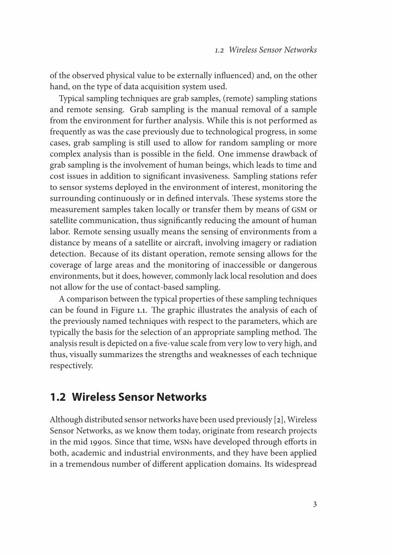
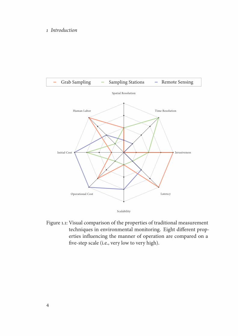
Typical sampling techniques are grab samples, (remote) sampling stationsand remote sensing. Grab sampling is the manual removal of a samplefrom the environment for further analysis. While this is not performed asfrequently as was the case previously due to technological progress, in somecases, grab sampling is still used to allow for random sampling or morecomplex analysis than is possible in the field. One immense drawback ofgrab sampling is the involvement of human beings, which leads to time andcost issues in addition to significant invasiveness. Sampling stations referto sensor systems deployed in the environment of interest, monitoring thesurrounding continuously or in defined intervals. These systems store themeasurement samples taken locally or transfer them by means of GSM orsatellite communication, thus significantly reducing the amount of humanlabor. Remote sensing usually means the sensing of environments from adistance by means of a satellite or aircraft, involving imagery or radiationdetection. Because of its distant operation, remote sensing allows for thecoverage of large areas and the monitoring of inaccessible or dangerousenvironments, but it does, however, commonly lack local resolution and doesnot allow for the use of contact-based sampling.
A comparison between the typical properties of these sampling techniquescan be found in Figure 1.1. The graphic illustrates the analysis of each ofthe previously named techniques with respect to the parameters, which aretypically the basis for the selection of an appropriate sampling method. Theanalysis result is depicted on a five-value scale from very low to very high, andthus, visually summarizes the strengths and weaknesses of each techniquerespectively.
1.2 Wireless Sensor Networks
Although distributed sensor networks have been used previously [2],WirelessSensor Networks, as we know them today, originate from research projectsin the mid 1990s. Since that time, WSNs have developed through efforts inboth, academic and industrial environments, and they have been appliedin a tremendous number of different application domains. Its widespread
3
1 Introduction
Time Resolution
Spatial Resolution
Human Labor
Initial Cost
Operational Cost
Scalability
Latency
Invasiveness
Grab Sampling Sampling Stations Remote Sensing
Figure 1.1: Visual comparison of the properties of traditional measurementtechniques in environmental monitoring. Eight different prop-erties influencing the manner of operation are compared on afive-step scale (i.e., very low to very high).
4

1.2 Wireless Sensor Networks
application is a result of the general necessity for sensor technology in mea-surement, monitoring and control tasks, as well as the flexibility gained bythe combination of this sensor technology with wireless communication andsoftware-based processing.While the implementation of a Wireless Sensor Network is greatly de-
pendent on the application requirements of the task to be performed, afundamentally similar architecture among different WSNs remains. A Wire-less Sensor Network is composed of multiple wireless sensor nodes2, whichtypically combine sensing, processing and wireless communication capabili-ties. The hardware implementation of these sensor nodes is, in the majorityof cases, based on specific wireless sensor node platforms, which implementthe desired functionalities. Whereas other hardware platforms can providethe required functionalities (e.g., mobile phones), wireless sensor node plat-forms are more specifically designed with the restrictions and requirementsof Wireless Sensor Networks in mind.
Depending on the application scenario and the network topology that hasbeen selected, the individual sensor nodes will communicate with the othernodes (or a specific subset), in order to form the Wireless Sensor Network.Furthermore, the nodes within the WSN can have identical functionalitiesand tasks (i.e., a homogeneous WSN), or their tasks and functionalities canbe complementary (i.e., a heterogeneous WSN).The main property of a Wireless Sensor Network is its capability of per-
forming distributed sensing tasks within the same system. This enables aselection of features, which are not possible with a single device system.Typically applied examples of these features include
• Collection of sensor data at different times and locations.
• Transfer of data throughout the network to a remote location, whichis different to the location where the data was collected.
• Data fusion to deduct information, which cannot be obtained fromdata taken at a single location.
2In the remainder of this document the terms wireless sensor node, sensor node, wirelessnode and node will be treated synonymously, and will always refer to wireless sensornodes.
5

1 Introduction
In order to utilize these features fully, however, several generally desiredsystem constraints are imposed on Wireless Sensor Networks. Sensor nodes,for example, should be of a small physical size, which maintains their place-ment flexibility. The implementation of each node should require a low cost,so as to result in an economically feasible system cost even when large num-ber of nodes are required by the application. Moreover, sensor nodes should,at least to a large extent, operate in a maintenance-free manner.These constraints have an influence on the implementation of Wireless
Sensor Networks. As a result, the typical node platforms are resource-limiteddevices, which allows for their cost and power consumption to bemaintainedat a low level. This, in turn, enables networks with a high number of sensornodes, but which require an optimization of the necessary functions to beperformed, to match the available resources.Although Wireless Sensor Networks can be used in many different appli-
cation scenarios and, thus, can be perceived as different types of systems,this document will treat WSNs as a measurement instrument. Furthermore,the remainder of this document will be restricted to the utilization of thismeasurement instrument in the domain of environmental monitoring.
1.2.1 Environmental Monitoring withWireless SensorNetworks
Environmental monitoring applications are based on the development fromdata to information to knowledge [1]. Hence, the more meaningful datathat is obtained, the more knowledge that can be derived. Because data isgathered through measurement and observation, the measurement systemcapabilities of WSNs offer several advantages to the field of environmentalmonitoring. Probably the most fundamental is the autonomy of data ag-gregation. While traditional sampling methods demand increased laborinput for larger amounts of samples (e.g., sampling at several locations in thesame area), an ideal WSN observes the environment at multiple locations andautomatically transmits the data to a gathering point via the networked infras-tructure. Furthermore, the autonomous sampling allows for the unobtrusiveobservation of phenomena and for monitoring in harsh locations and underextreme conditions [3]. Because the sensing networks are usually directlyconnected to the operator via the Internet or some type of local connection,
6
1.2 Wireless Sensor Networks
data is gathered in real-time or near-real-time. This enables problems tobe detected at an earlier stage than would be possible in systems with localstorage and manual downloading at the end of an acquisition period. Inaddition, the remote connection to the sensor network means the removalof distance between the scientist and the monitored site [3], as the researchercan directly observe what is happening at a particular area of interest.
Nevertheless, environmental monitoring is an extensive area and differentapplications impose different requirements on the Wireless Sensor Network.A rough, but useful, classification ofWSN-applications ismade by Barrenetxeaet al., who divide these systems into time-driven, event-driven and query-driven sensor networks [4]. However, as sensing in most applications istime-driven (e.g., by continuous or periodically sampling of the attachedsensing devices), the classification mainly describes the communicationactivity in the system. Within these, time-driven applications usually transmittheir sensor readings periodically, which is typically used in data gatheringapplications, such as [5, 6]. However, event-driven sensor networks attemptto minimize the actual ongoing traffic and the flooding of the gatheringpoint with meaningless information. These types of systems observe the areaof interest, transmitting sensor information only on those occasions whenparticular events occur, such as a fire [7] or volcanic eruption [8]. Query-driven systems store gathered information locally and communicate it onrequest. This type of sensor network can, for example, be useful in logisticsor home applications, but is not very common in applications relating toenvironmental monitoring.
The system requirements of the different application classes differ tremen-dously. While it is the case that time-driven sensor networks are usually morepredictable, especially in terms of network traffic, event-driven applicationsbehave more randomly and in an unforeseeable manner. Because of thesedifferences, it is not usual for system designs, particularly in communicationprotocols, for both classes to be interchangeable. Therefore, the presentedwork in this document is limited to time-driven applications in the environ-mental monitoring domain. A more detailed definition of the applicationscenario, which is targeted by this work, is described below.
7

1 Introduction
1.2.2 Application Scenario under Scope
Due to the broad applicability of Wireless Sensor Networks, as well as itshighly application-specific implementation, this section is used to define thetype of applications addressed by the work that is presented in the remainderof this document. While a large set of design parameters has beenmade basedon the application scenario under scrutiny, the majority of presented resultscan, directly or with slight modifications, be utilized in other applicationscenarios within the WSN design space.The application scenario primarily addressed in this work involves data
gathering Wireless Sensor Networks. These applications are manifold in thefield of environmental monitoring and are usually used to aggregate largesets of data, which originate at different locations over an extended period oftime. According to the WSN taxonomy introduced by Mottola et al. in [9],these applications are referred to as sample-and-send applications. Examplesinclude studies of water quality [10], microclimates of glaciers [4, 11] orrainforests [5], as well as the measurement of light intensity under shrubs [12].The data collected in these applications is typically utilized as the input inorder to provide a better understanding, modeling or site status observation.An additional restriction is made in the manner that the focus lies on
time-driven applications, where physical values are measured and gatheredcontinuously (or semi-continuously). As opposed to the event-driven sensornetworks, time-driven systems possess only limited data processing withinthe sensor node units. While event-driven applications communicate theoccurrence of events, and therefore, in the majority of cases, require to trans-late data into information before any communication can occur, time-drivenapplications typically transfer pure sensor data. The drawback associatedwith time-driven applications is in relation to their increased amount ofcommunication, which is, in most implementation forms, more costly thanprocessing. Using WSNs in environmental monitoring as a scientific mea-surement tool, however, provides the low-level sensor data with increasedvalue.
As a result of this, typical wireless sensor nodes in the network can be rathersimple devices, thus reducing system complexity, size and cost. Additionally,large amounts of these simple devices are necessary in order to cover large-scale areas, while maintaining the required spatial resolution. The number
8

1.2 Wireless Sensor Networks
Sensor nodes
Clusterheads
Gateway
Data server
Node communication
Clusterhead communication
Global communication
Figure 1.2: An overview on the typical network architecture of environmen-tal monitoring applications under scope. The network topologydepicted only serves as an example.
of nodes opens up several challenges which must be addressed in theseapplications, such as the handling and visualization of data, communicationand configuration protocols, as well as the deployment and maintenance ofthe network. Further details with reference to these research challenges willbe given in Section 1.5.
Figure 1.2 shows a possible network architecture for data gatheringWSNs inenvironmental monitoring, and the type of network architecture we addressin this work. As many environmental monitoring systems are deployed inremote locations (or at least at a distance from the operator), a distinctionbetween the local and global domain is made. The local sensor field containsthe sensor nodes, which are monitoring the deployment site, while beingindirectly connected to the global domain via some kind of gateway (i.e., alocal to global communication translator).In the depicted architecture example, the sensor field is organized in a
9

1 Introduction
cluster-star topology, which requires two different node types, namely, clusterheads and end nodes. Although this is not the sole implementation option,several design considerations have led us to the belief that this is an appro-priate choice for the application at hand. Details on the motivation for thisarchitectural choice will be given in Section 2.5.
The global domain usually includes a data processing and storage unit, suchas a data server. From here, data is converted into a representable form andmade available to the operator of the network and environmental researchers,typically via the Internet. Based on the distance between the sensor field andthe data storage that can be found in the majority of WSNs, the link betweenthe local and global domain is, in many cases, implemented using long-distance communication technologies, such as GSM/GPRS. In other cases, apure translation from the communication methods used within the WirelessSensor Network to those used in computer networks may be sufficient.
1.3 Case Study - SAQnet
SAQnet (Sundsvall’s Air Quality network) has been an experimental applica-tion for the usage of Wireless Sensor Networks in environmental monitoring,which has been conducted at Mid Sweden University during 2011. The resultsthat have been obtained from conducting this project were twofold. Onthe one hand, experiences on the general – and also application-specific –development and deployment of WSN systems has been gained. On the otherhand, the application scenario has been used in order to evaluate the state ofthe art off-the-shelf sensor network equipment. These results have supportedthe research decisions that have been made prior to this study, as well asproviding new directions, which have subsequently been addressed. Thus,this case study acts as a motivator towards the study of the research problem,which is formally stated in Section 1.5.
The case study is presented in the next two sections. Firstly, Section 1.3.1will provide the technical background, which includes the motivation, archi-tectural choices and the implementation of the application. Then, in Section1.3.2, the experiences and analysis results of the development and final systemwill be presented. We will finally establish a link between these results andopen research problems within the area of WSNs.
10

1.3 Case Study - SAQnet
1.3.1 Background, Architecture and Implementation
As a result of urbanization and industrialization, the amount of air pollu-tants produced by human sources increases and the majority of the worldpopulation is exposed to these pollutants on a daily basis. The monitoring ofthe air quality becomes a crucial activity in order to establish and maintainregulatory thresholds, which will protect us from harmful consequences.Furthermore, monitoring can be used to analyze the production and distri-bution processes of the air pollutants, as well as to relate the concentrationsto external parameters. Because the pollution levels are affected by internalparameters (e.g., the number of cars driving on a road), as well as externalparameters (e.g., the wind speed and direction), they have high spatial andtemporal variations. While currently applied monitoring stations providehigh accuracy and a good temporal resolution, a sufficient spatial resolutionis rarely accomplished, which is a result of their high monetary costs. Apply-ing WSN technology allows there to be an increase in the spatial resolutionof air pollution monitoring, however, typically at the cost of per-locationsampling accuracy.
In order to establish a measurement of the outdoor air quality, the param-eters to be monitored in the SAQnet system are primarily gas concentra-tions. Nevertheless, temperature and humidity levels have been collectedas reference parameters alongside the gas level measurements. The systemarchitecture follows a standard sample-and-send scenario as described inSection 1.2.2. The resulting system design can, therefore, be split into threesystem layers, which are the sensing layer, the storage layer, and the dataaccess layer. This layered system organization, together with the componentseach layer consists of, is depicted in Figure 1.3.The actual monitoring task is performed by a number of sensor nodes,
which collect a set of environmental parameters in a time-driven manner.The design of these nodes follows a rather conventional architecture, whichcontains a low-power microcontroller, a Radio Frequency (RF) transceiver,sensors, and a battery-based power supply (see Figure 1.4). As was previouslymentioned, the system implementation was intended to be largely based onoff-the-shelf equipment. Thus, the sensor node has been implemented onthe basis of a commercial node platform. Table 1.1 lists the individual imple-mentation choices for the node’s components. As relatively long distances
11

1 Introduction
GUI
Data Access
Data Storage
Sensing
Web Interface
Management Gateway Database
Sensor Node Sensor Node Sensor Node ...
Figure 1.3: The abstracted architecture of the SAQnet system, divided intothree functional layers.
Low-Power Microcontroller
Battery-based Power Supply
802.15.4 Radio Transceiver
CO2CO
NO2
HT
Sensors
Figure 1.4: The high-level architecture of an SAQnet node. Each node in-cludes computing, communication, sensing and power modules.
between sensor nodes were expected, an RF module with increased outputpower was chosen. This enables there to be a coarser node deployment at thecost of an increased communication power consumption. The selection of thesensors has been based on parameters of interest in air pollution monitoring,as well as the sensor availability for the chosen node platform. Furthermore,the initial node design did use a high capacity primary battery as its energysource (i.e., power option A in Table 1.1). Based on the limitations in theresulting node lifetime, however, an alternative power option has been con-sidered, which is based on a secondary battery in connection with a 2.5Wsolar panel. A more detailed description of the underlying reason for theselection of an alternative power supply will be provided at a later stage.
In order to make use of the sensor data that is sampled by the sensor nodes,
12

1.3 Case Study - SAQnet
Module Description Implementation
Computing/Control Platform LibeliumWaspmoteCommunication Radio Module Digi XBee 802.15.4 PRO
Sensing
Temperature Microchip MCP9700AHumidity Sencera 808H5V5CO Figaro TGS2442CO2 Figaro TGS4161NO2 e2v MiCS-2710
Power (Option A) Primary Battery Saft LSH20 3.7 V – 13Ah
Power (Option B) Secondary Battery Li-Ion 3.7 V – 6.6AhSolar Panel 12V - 200mA
Table 1.1: Implementation details of the modules in a SAQnet node.
the data has to be collected, stored, and made available for user access. Forthis purpose, a gateway node has been implemented, which receives the dataof each node and stores it in a MySQL database. The implementation ofthe gateway is based on the Meshlium platform3, which operates on a x86processor. This allows for the usage of standard PC-class operating systemswith their respective libraries. The platform, furthermore, provides Ethernetand WLAN, which enables the system to be connected to an TCP/IP network,and, thus, an easy interface to the Internet.Using the TCP/IP connection, two different user interfaces have been
designed. Firstly, data can be accessed from a web interface, which is mainlyintended for the end user of such a system. The data obtained from thedifferent sensors and locations is visualized and can be compared based ondifferent parameters. The implementation of a web interface was selectedin order to allow a simple and uniform interaction with the system, whichdoes not require a special software installation and can be performed fromany location. In order to perform system maintenance, which normal usersshould not have access to, a Graphical User Interface (GUI) program hasbeen implemented. In addition to the data inspection that can also be per-formed with the web interface, the GUI allows for maintenance tasks, such as
3http://www.libelium.com/products/meshlium/
13
1 Introduction
Node
Node
Node
Node
Node
Gateway
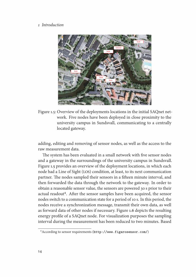
Figure 1.5: Overview of the deployments locations in the initial SAQnet net-work. Five nodes have been deployed in close proximity to theuniversity campus in Sundsvall, communicating to a centrallylocated gateway.
adding, editing and removing of sensor nodes, as well as the access to theraw measurement data.
The system has been evaluated in a small network with five sensor nodesand a gateway in the surroundings of the university campus in Sundsvall.Figure 1.5 provides an overview of the deployment locations, in which eachnode had a Line of Sight (LOS) condition, at least, to its next communicationpartner. The nodes sampled their sensors in a fifteen minute interval, andthen forwarded the data through the network to the gateway. In order toobtain a reasonable sensor value, the sensors are powered 30 s prior to theiractual readout4. After the sensor samples have been acquired, the sensornodes switch to a communication state for a period of 10 s. In this period, thenodes receive a synchronization message, transmit their own data, as wellas forward data of other nodes if necessary. Figure 1.6 depicts the resultingenergy profile of a SAQnet node. For visualization purposes the samplinginterval during the measurement has been reduced to two minutes. Based
4According to sensor requirements (http://www.figarosensor.com/)
14

1.3 Case Study - SAQnet
0 50 100 150 200 2500
40
80
120
160
Sen
sing
Com
mun
icat
ion
Sle
ep
Time [s]
Cur
rent
Con
sum
ptio
n [m
A]
Figure 1.6: Energy profile of a SAQnet node, which runs a 2min periodicsampling configuration. Contributions to the consumption aremarked with their respective tasks.
on a fifteen minute interval, the average current draw can be estimated to5.35mA, of which sensing clearly consumes the largest part.As a result, the battery powered sensor nodes in the network showed a
lifetime of between 9 days and 34 days, which was considerably shorter thana back-of-the-envelope calculation would suggest (i.e., approximately 100days). The solar powered sensor node, on the other hand, has been providingsensor readings uninterruptedly since its initial deployment.
1.3.2 Project Analysis
In addition to the data that has been collected by the sensor nodes, the systemdevelopment and implementation did provide insights and experiences withrespect to the application of WSNs in the environmental monitoring domain.These qualitative results, which have mainly been gained from dealing withdesign and implementation challenges, have indicated unsolved problems inthe technology to be applied. The main experiences made, which concernboth application-specific and general design considerations, are listed below.
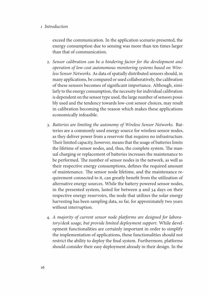
1. Sensing can significantly contribute to energy consumption in wirelesssensor nodes. While in many applications, simple sensors might besufficient, which results in the communication being the major energyconsumer of the node, this is not always the case. Depending on thesensor types used, the energy consumption due to sensing can easily
15
1 Introduction
exceed the communication. In the application scenario presented, theenergy consumption due to sensing was more than ten times largerthan that of communication.
2. Sensor calibration can be a hindering factor for the development andoperation of low-cost autonomous monitoring systems based on Wire-less Sensor Networks. As data of spatially distributed sensors should, inmany applications, be compared or used collaboratively, the calibrationof these sensors becomes of significant importance. Although, simi-larly to the energy consumption, the necessity for individual calibrationis dependent on the sensor type used, the large number of sensors possi-bly used and the tendency towards low-cost sensor choices, may resultin calibration becoming the reason which makes these applicationseconomically infeasible.
3. Batteries are limiting the autonomy of Wireless Sensor Networks. Bat-teries are a commonly used energy source for wireless sensor nodes,as they deliver power from a reservoir that requires no infrastructure.Their limited capacity, however, means that the usage of batteries limitsthe lifetime of sensor nodes, and, thus, the complete system. The man-ual charging or replacement of batteries increases the maintenance tobe performed. The number of sensor nodes in the network, as well astheir respective energy consumptions, defines the required amountof maintenance. The sensor node lifetime, and the maintenance re-quirement connected to it, can greatly benefit from the utilization ofalternative energy sources. While the battery powered sensor nodes,in the presented system, lasted for between 9 and 34 days on theirrespective energy reservoirs, the node that utilizes the solar energyharvesting has been sampling data, so far, for approximately two yearswithout interruption.
4. A majority of current sensor node platforms are designed for labora-tory/desk usage, but provide limited deployment support. While devel-opment functionalities are certainly important in order to simplifythe implementation of applications, these functionalities should notrestrict the ability to deploy the final system. Furthermore, platformsshould consider their easy deployment already in their design. In the
16

1.3 Case Study - SAQnet
Figure 1.7: A packaged SAQnet node. While optimized for laboratory usage,preparing the node for an outdoor application can be challenging.
SAQnet deployment an example of this was the connection of sensors.The waspmote platform provides interfaces to sensors via the so calledsensor boards. In order to connect sensors to these boards, they con-tainmultiple sockets, which aremainly composed of standard 2.54mmheaders. While this allows for the easy connection of sensors in thelaboratory (i.e., they are just placed inside the sockets), preparing thenode for deployment becomes tremendously difficult, because sensorshave to be wired to these connectors (see Figure 1.7).
5. Wireless Sensor Networks do not provide sufficient end user interfaces.The design, implementation and operation of Wireless Sensor Net-works requires a considerable technical understanding by their endusers. The typical end users of such a system, however, are domain ex-perts (i.e., in the environmentalmonitoring domain biologists, chemists,farmers, etc.). It is not uncommon for these end users not to possessthe required skills in order to independently work with WSNs. In themajority of existing deployments, this has led to a collaborative workbetween domain experts and system experts and it is due to theircommon interest in gaining experiences with these systems, that thiscollaboration has been possible. Over time, however, the interest inutilizing the system will shift towards the end users, which will lead toadditional costs if a system support remains a requirement.
17

1 Introduction
1.4 Application Analysis
Application oriented development has been a common methodology in WSNresearch and, thus, a plethora of different applications of Wireless Sensor Net-works have been reported in the literature. Table 1.2 presents the analysis ofa subset of these applications based on the experiences we have encounteredin the SAQnet application (see Section 1.3.2).
The selection of the ten projects has been based onmultiple criteria. Firstly,all of the presented applications are in the application domain of environmen-tal monitoring. Secondly, the applications are, from a application scenariopoint of view, close to the application scenario, which is addressed in thiswork. In order to determine this application similarity, the WSN taxonomyintroduced in [9] has been applied. According to this taxonomy, all presentedapplications are sense-only application with amany-to-one interaction. Fur-thermore, they are static and data collection occurs in a periodic manner.Finally, applications have been selected based on their level of detail withrespect to the description of parameters of interest. These applications havebeen analyzed with respect to their system lifetime and their usability inrelation to the intended end users, as these parameters represent the generalissues of those that have previously been described.Although usability, as a qualitative design parameter, is rarely evaluated
in the presented works, its influence can be determined from the mannerin which the applications have been conducted. All of the applications thathave been presented, have been performed collaboratively by system expertsand domain experts. In this collaboration, the system experts have beenthe provider and the domain experts the consumer of the measurementdata. While the domain experts, thus, have been the end user of the WSNsystem, they have, in none of the presented scenarios, been the operator ofthe system. Martinez et al. state this as an issue to be addressed, in order todevelop Wireless Sensor Networks to become a competitive technology ascompared to the state-of-the-art measurement methods in environmentalsciences [13, chap. 9].Despite their differences with regards to their sampling intervals, which
are ranging from continuous sampling to a few sensor readings per day, themajority of application examples list lifetime as a restricting system parameter.While the systems operating on solar energy have overcome this limitation
18

1.4 Application Analysis
Application
Syste
mOperator
EndUser
SampleP
eriod
Energy
Source
Lifetim
eRestrictio
nRe
ported
Lifetim
e
HabitatM
onito
ring[14,15]
Syste
mEx
pert
Biolog
yMinutes
Batte
ries
yes
days
tomon
ths
Glacier
Mon
itorin
g[16,17]
Syste
mEx
pert
Geography
Hou
rsBa
tterie
sno
mon
thstoyears
Potato
Mon
itorin
g[18]
Syste
mEx
pert
Agriculture
Minutes
Batte
ries
yes
weeks
VolcanoMon
itorin
g[8,19]
Syste
mEx
pert
Geoph
ysics
Con
tinuo
usBa
tterie
syes
hourstoweeks
SensorScop
e[4,6]
Syste
mEx
pert
Hydrology
Minutes
Solar+Ba
tterie
sno
–Re
dwoo
dTree
[20]
Syste
mEx
pert
Biolog
yMinutes
Batte
ries
yes
weeks
SoilMon
itorin
g[13,chap.6]
Syste
mEx
pert
Biolog
yMinutes
Batte
ries
yes
weeks
Cane
Toad
Mon
itorin
g[21]
Syste
mEx
pert
Zoolog
yCon
tinuo
usBa
tterie
syes
–Lu
ster[12]
Syste
mEx
pert
Biolog
ySecond
sBa
tterie
syes
hourstoweeks
Sprin
gbrook
[5]
Syste
mEx
pert
Ecolog
yMinutes
Solar+Ba
tterie
sno
–
Table1.2:
Analysis
results
ofexistingapplications
inthee
nviro
nmentalm
onito
ringdo
main.
Thes
electionprocess
hasb
eenbasedon
thea
pplications’sim
ilarityto
thea
pplicationscenario
addressedin
thiswork.
19
1 Introduction
by replenishing their energy reservoir, only one battery powered systemreports node lifetimes in the order of years [16, 17]. This, however, is onlyachieved by greatly reducing the sampling rates as compared to the otherapplications. The discrepancy between the expected and the actual nodelifetime, which has been experienced in the SAQnet deployment, has beenconfirmed multiple times, such as in [15, 18].As a result, the end user interface and the system lifetime prove to be
general constraints in the field ofWireless SensorNetworks for environmentalmonitoring applications, as opposed to being an application-specific concern.Furthermore, solar energy harvesting has been demonstrated repeatedly as acomplementary solution in order to extend the lifetime of battery-powered,outdoor Wireless Sensor Networks.
1.5 Problem Formulation
Wireless Sensor Networks have the possibility to become a newmeasurementstandard in environmental monitoring applications. Enabling autonomousmeasurements on a large scale, but possibly with a high spatial resolution,makes this technology an attractive solution for manifold problems.
A distributed measurement system, which is composed of a large numberof individual but connected devices, however, does not only increase theapplication possibilities in the environmental monitoring domain, but posesa number of system challenges. These challenges need to be addressed andsolved in order for WSNs to fulfill their promised vision. During two decadesof system research, WSN technology has been developed considerably. Today,low-power platforms can be bought at low cost, and standardized communi-cation protocols can be obtained from multiple sources. While this allowsfor an overall low equipment cost, the operational costs of a sensor networkremain high, due to the reappearing challenges of end user interfaces andthe system lifetime (see Section 1.4).Although lifetime demands can vary from application to application, a
long system lifetime is desirable in most application scenarios in order toreducemaintenance requirements. Themajority of implemented applications,however, have demonstrated system lifetimes of the order of weeks (see Table1.2). In combination with the possibly large number of nodes, this lifetime
20

1.6 Thesis Contributions
restriction leads to high maintenance requirements and, thus, makes theapplication of battery-based Wireless Sensor Networks in the majority ofscenarios, economically infeasible.
The utilization of solar energy harvesting can increase the lifetime of sensornodes within the network and, thus, increases the lifetime of the networkitself. However, this solution will lead to an increase in size and cost of thesensor nodes. The implementation of a solar energy harvesting system shouldtherefore be well dimensioned in order to limit the additional size and costto an appropriate level.The second influencing factor with regards to the operational cost is sys-
tem support. In environmental monitoring applications, the provider andend user of the measurement system are typically not the same. In existingapplications, this has been only a limited problem, as the applications havebeen conducted collaboratively, which means that the system provider wasresponsible for the system operation. This, however, has only been an op-tion because system experts have been interested in the development andadvertisement of WSNs, and, thus, have been funded from their own sources.As Wireless Sensor Networks mature, this interest will decrease and this, inturn will mean that the end users will have to pay for any system support, or,in order to avoid the additional costs, be capable, themselves, of operatingthe system. End user interfaces are therefore an important part of system de-sign, in order to develop WSNs into a economically competitive measurementinstrument.
1.6 Thesis Contributions
In this thesis, both the lifetime restriction and the system usability, havebeen addressed in order to reduce the operational cost of Wireless SensorNetworks as a measurement instrument. As parts of this research problemhave been previously targeted, and is too broad to be solved as a whole, thefollowing list provides the main contributions from this work:
1. Analysis and design of a low-power hardware platform for the imple-mentation of wireless sensor nodes with respect to their lifetime anddevelopment usability. (Paper II)
21

1 Introduction
2. Analysis and experimental verification of synchronized communica-tion as a method to reduce overall energy consumption by allowingefficient resource use, such as low duty cycles. (Paper III)
3. Investigation of micro-scale energy harvesting architectures with afocus on solar energy harvesting in locations with challenging lightconditions. (Paper IV)
4. Experimental evaluation of short-term energy storage devices in solarenergy harvesting architectures for low-power wireless sensor nodes.(Paper V)
5. Proposition, implementation and analysis of energy level simulationsas a tool for dimensioning solar energy harvesting systems. (Paper VI)
6. Design and evaluation of a solar energy harvesting testbed, in order tosimplify the comparison of harvesting architectures and the generationof input data for the development of respective simulation models.(Paper VII)
7. Design and implementation of a framework for the programmingof wireless sensor nodes based on finite state machines in order toimprove development usability for experienced users. (Paper VIII)
8. Implementation and analysis of a method for the programming ofwireless sensor nodes by non-technical end users. (Paper IX)
1.7 Thesis Outline
The remainder of this thesis is divided into four chapters. Chapter 2 addressesthe energy efficiency of wireless sensor nodes. After an analysis of the lifetimeconstraints in WSNs and the contributions of node modules and tasks to theenergy consumption of the system, a sensor node design with the focus onenergy efficiency is presented. Furthermore, energy efficient communica-tion based on synchronous task scheduling is proposed. An appropriatesynchronization protocol with low communication overhead is presentedand experimentally evaluated.
22

1.7 Thesis Outline
Chapter 3 deals with the utilization of solar energy harvesting for theimprovement of sensor node lifetime. While, particularly, battery-basedsystems have been used before, the focus of this chapter lies on short-termenergy storage based architectures to be analyzed. A number of architecturesis experimentally compared and analyzed. Moreover, the modeling andsimulation of respective architectures is addressed in order to allow for thesystems to be dimensioned with respect to individual application constraints.Finally, a method, which uses an adapted testbed approach, is introducedin order to allow for systematic experimentation and data generation to beperformed.The usability of sensor node devices is addressed in Chapter 4. An ar-
gument is made for the division of usability development with respect todevelopers and system end users. The presented contributions contain aprogramming method for technically-experienced developers, which uti-lizes the concept of Finite State Machines (FSMs) in order to improve thesystematic and modular development of sensor node software. In addition,sensor node considerations for the improvement of usability are presentedand demonstrated on the implementation of a sensor node platform. Finally,end user usability is addressed by the development and implementation of aspecification-based configuration approach.
In Chapter 5, the presented contributions are summarized and discussed.Furthermore, conclusions based on the presented results are made.
23


2 Energy Efficiency
In this chapter, the lifetime of aWireless Sensor Network will be addressed interms of the energy efficiency of sensor node operation. We will present ananalysis of the lifetime constraints, as well as influencing factors in relationto the lifetime on a sensor node level. In order to improve the lifetime, ourcontributions address the energy efficiency of task execution on both thehardware and software level.
2.1 Wireless Sensor Network Lifetime
As described in the previous chapter, WSNs enable autonomous sensing on alarge scale. Ideally, a large number of sensor nodes are spread over a widearea (possibly at a remote or harsh location), organizing themselves andcommunicating their sensor data back to the researcher without furtherattendance. A key parameter for allowing the nodes to fulfill this task is thatthere must always be a sufficient energy supply. If the system demands theuser to re-visit the deployment site too frequently, in order to exchange orreplenish the systems’ energy reservoirs, this defeats the initial advantagesoffered by the system in the first place.Because of the importance of the system lifetime in the final application,
lifetime has been used extensively as an evaluation parameter in the designsat all levels in sensor networks. However, providing a definition for theWSN-lifetime at a general level is very difficult. Several definitions have beenproposed in the literature and a comprehensive coverage of these definitions(or definition-classes) is given in [22].
A first classification is usuallymade by separatingWireless Sensor Networklifetime from sensor node lifetime. While these two parameters are typicallyconnected to each other, they have to be targeted on different levels.Sensor node liveliness can usually be determined directly from the oper-
ational status of a sensor node at a given time. Typically, the lifetime of a
25

2 Energy Efficiency
sensor node is defined by its energy reservoir and its energy consumptionover time. Limited energy resources are, thus, the only limiting factor forthe nodes lifetime (ignoring hardware defects at this point). Nevertheless,operational interruptions can certainly occur during the lifetime of a sensornode, which might require additional consideration.In comparison, WSN lifetime is not as easy to determine without taking
more application constraints into account. Typical definitions are based onthe availability of sensor nodes, the coverage of the monitored terrain or theconnectivity of the network. In addition, combinations and extensions ofthese factors might also be placed into the definition of a sensor networklifetime [22]. Since sensor nodes are the building blocks of Wireless SensorNetworks, their lifetimes are connected, but the extent of this connectioncan vary from application to application.Different scenarios regarding the WSN lifetime definition based on oper-
ating sensor nodes include the n-of-n, k-of-n orm-in-k-of-n scenarios. Thefirst two cases are straightforward solutions, where n-of-nmeans all nodeshave to be alive, while in k-of-n at least k-nodes have to be alive. If the caseis not met because more nodes are dead than are allowed, then the lifetimeof the entire sensor network is considered as being ended. Different sensornodes, however, can have tasks with different significance to the system theyare operating in. A node that regularly forwards data of other nodes, shows alarger significance to the network than an end node. These cases are includedin anm-in-k-of-n scenario, in which at leastm critical nodes (e.g., routers)out of k remaining nodes are required for the task execution.Although WSN lifetime is typically the final parameter of interest, due to
its application dependency, the remainder of this document will address thesensor node lifetime. However, based on the link between sensor node life-time and system lifetime, WSN lifetime is addressed indirectly. Furthermore,we will limit the focus of the sensor node lifetime to the availability of energy.
2.2 Wireless Sensor Node Architecture
The basic architecture of wireless sensor nodes has not changed significantlysince the initial proposal of WSNs. It usually contains modules for computa-tion, communication, sensing and power management. Application-specific
26

2.2 Wireless Sensor Node Architecture
tasks can require some additional resources, but in the majority of cases thesefunctionalities can be classified as belonging to one of the basic modules,mentioned previously. An abstract overview of the hardware architecture ofgeneral sensor nodes is provided in Figure 2.1.The computation module of a sensor node usually has several tasks to
fulfill. It controls the other components on the platform, processes and storesdata, and provides an interface to the user/programmer. While the imple-mentation of the computational module will truly depend on the specificapplication, the majority of nodes implement the computation module basedon a low-power microcontroller. Microcontrollers integrate a variety of differ-ent hardware modules, which are useful for the accomplishment of the sensornode tasks. Furthermore, they are easily programmed and have low powerdemands. Popular choices in existing sensor nodes include Atmel’s ATmegaseries [23, 24], Texas Instruments MSP430 [25–27], as well as PIC controllersfromMicrochip [28]. For processing intensive applications, however, FieldProgrammable Gate Arrays (FPGAs) and Digital Signal Processors (DSPs)might be used as co-processors [29].Because an active operation consumes a considerable amount of power
(i.e., normally of the order of hundreds of μAMHz−1), most microcontrollers
Computation,Control and
Storage
Power Management
Communication
Sensing
Data
Pow
er
Pow
er
Figure 2.1: Abstracted architecture of typical sensor nodes, used in Wire-less Sensor Networks. These nodes typically combine processing,communication and sensing capabilities, and are powered by anenergy source (e.g., a battery)
27

2 Energy Efficiency
offer a series of operating modes, allowing the system to conserve energywhen activity is not required. Nonetheless, to allow this operation, the mi-crocontroller must facilitate the means to be woken up again in order tocontinue the normal operation when necessary.In a similar manner to the computational module, the communication
module implementation also depends to some degree on the application.Nevertheless, it is also the case that the majority of systems use similar com-munication devices, namely low-power RF transceiver, typically operating inthe license-free ISM-band. Other communication methods, such as acousti-cal or optical techniques are only used in special cases (e.g., for underwatersensor networks). While RF has been a popular communication methodsince the early stages of WSN research, over the last few years transceiversthat are compatible with the IEEE 802.15.4 protocol1 have become the de-factocommunication standard. This is partly due to its world-wide available fre-quency band, as well as the increased interest in commercialization, which ispositively affected by applying a standardized communication protocol.The main task for the communication module is the establishment of a
link between individual nodes. This link, in turn, is used in order to exchangedata between sensor nodes, and, particularly in environmental monitoringapplications, in order to propagate data from the individual sensor nodes toa central data collection unit (i.e., the network sink). In addition to this localcommunication link, a global communicationmodulemight be implemented.This module has the purpose of connecting the local sensor network to theoutsideworld and, thus, provides a universal accessmethod to themonitoringsystem. Typical implementations of this global communication module areWiFi [14], long-range radio communication [8, 11] and GSM/GPRS [5, 20].However, the number of nodes that are equipped with such a module isstrictly limited, as both the power consumption and the price for thesedevices are excessive.
Although themajority of sensor nodes within the system only contain localcommunication, communicating remains costly for these resource limiteddevices. Evenwhen operating in idlemode, and only listening to surroundingnoise, energy consumption of the communication module is tremendous,easily reaching similar levels to those involved in transmitting data. Therefore,
1http://www.ieee802.org/15/pub/TG4.html
28
2.2 Wireless Sensor Node Architecture
sensor nodes should disable their communication modules whenever possi-ble, reducing power consumption by several orders of magnitude. However,waking up in time to receive a packet destined for this node can become aconsiderable problem.
While the implementations of computation and communication modulesvary depending on the resource requirements of the application, it is definitelythe case that the most application-specific part of a sensor node is its sensingmodule. A given application will be required to monitor certain physicalparameters or detect specific events. This, in turn, requires specific sensorsthat have the ability to fulfill these application demands.Although any type of sensor is imaginable for WSN operation, the choice
of sensors found in the literature is rather limited. The majority of work islimited to low-power sensors, with a typical example being temperature sens-ing. The possible reasons for this are, limited application-oriented research,difficulties in performance comparison when there are different underlyingassumptions, as well as the simplicity and availability of these sensing devices.Nonetheless, this easily leads to assumptions within the community that donot generally hold true. One typical example being the negligible energyconsumption of the sensingmodule. While this might hold true for the abovementioned temperature sensors, there are many sensors that have a higherpower consumption than the communication module or require tremendouswarm-up times in order to provide accurate readings. The presentation ofthe SAQnet deployment in Section 1.3 provides an example in this regard.
While it is typically not considered to be a main function of a sensor node,underlying all other node modules is the power supply. Its main task is assimple as it is important, namely in providing a stable power supply to allactive components of the sensor node system. This means that it convertsthe input from the energy source to acceptable levels in order to power theconnected devices.The manner in which this conversion actually appears will generally de-
pend on the type of energy source used for the sensor nodes. In some casesthe sensor node might be able to extract power from a power grid, requiringa module for AC-DC conversion. However, especially in environmental mon-itoring WSN applications, this is seldom the case. The use of battery suppliesis more popular, and, recently, the use of harvesting energy from ambientenergy sources, such as wind, temperature difference or the sun has gained
29

2 Energy Efficiency
increased interest [30, 31]. For these sources, the power supply is based onDC-DC converters.Additionally, the power module might include monitoring and control
functions. The type of monitoring is mainly dependent on the energy sourcein use. For example, in the case of a battery-based source, a typically desiredmonitoring function to be implemented is the determination of the battery’sState-of-Charge (SOC) in order to predict, for example, its remaining life-time. On the other hand, for energy harvesting systems, the observation ofthe incoming energy level might be more important, due to its intermittentbehavior. Control functions are implemented, for example, to react to moni-tored events or periodic tasks. A typical example is the shutdown of certainmodules on the node in order to conserve energy, either because they areunnecessary or because reduced energy income was detected. In case thesemodules do not have own low-power modes, or their quiescent current istoo large, the power supply module can contain features in order to disablethe modules.
2.3 Duty-Cycling
As mentioned previously, most active components (e.g., microcontroller andRF transceiver) provide multiple power states, with tremendous differencesin their energy consumption. In reality, the choice of operation states canbe quite broad. For example, a typical MSP430 microcontroller2 from TexasInstruments offers seven different states (i.e., one active mode, five low powermodes, as well as shutdown), thus allowing the optimization of energy con-servation by picking the most appropriate operation mode at any given time.However, for simplification reasons, in the following, a division will onlybe made between active state and inactive state. This will provide the basicunderlying principles, that can be extended by means of further operationstate layering when required.
Duty-cycling is a common approach for the reduction of the average energyconsumption of wireless sensor nodes. Its main principle is to achieve lowerenergy consumption by reducing the power levels whenever possible (seeFigure 2.2 for a graphical representation). Defining the portion of time in2http://www.ti.com/product/msp430fg4618
30

2.3 Duty-Cycling
Time
Pow
er
TA TI
T
Figure 2.2: Graphical representation of the duty-cycling principle (simplifiedfor bi-modal operation states)
the active state as Tactive and the period in the inactive state as Tinactive , theduty cycle δ can be formally described as
δ = TactiveTactive + Tinactive
, 0 ≤ δ ≤ 1 . (2.1)
In order for the method to be effective, the duty cycle δ should be consider-ably smaller than one. Furthermore, the respective active and inactive stateshave to differ in their power consumption levels. In typical WSN applications,both requirements are fulfilled. Particularly in environmental monitoring,sampling rates are rather low (i.e., often in the order of minutes [3, 6, 32]).This leads to extremely low duty cycles in the network, which are oftenmuch smaller than one percent. The consumption level differences are ac-complished by toggling the individual sensor node modules between activeand inactive states. An overview of the current consumption levels usuallyachieved in different module states is given in Table 2.1. As a result, powerrequirement reductions of multiple orders of magnitude are not uncommonwhen disabling modules that do not perform a task.
Taking these factors into account, duty-cycling can be applied to the differ-ent consumers of the sensor node. In general, the average power consumptionof a duty-cycled sensor node can be described as
31

2 Energy Efficiency
Pδ = Pactive ⋅ Tactive + Pinactive ⋅ TinactiveT
(2.2)
= δ ⋅ Pactive + (1 − δ) ⋅ Pinactive . (2.3)
Herein, the interval time T is the sum of Tactive and Tinactive and δ asdescribed in Equation 2.1. However, for each sensor node module individ-ual challenges have to be addressed. The simplest of these is usually thecomputational unit, as it is the the central control unit in the system. Thecomputational unit, thus, can switch to a low-power mode whenever idle(i.e., waiting for the next event to occur). The only limitation being, thatit is possible to awaken the module from its low-power state as soon as anevent has to be processed, which is usually implemented by utilizing inter-rupts. The resulting power consumption can be estimated by substitutingcomputational unit values into equations 2.2 and 2.3
State
Module Operation Classifier Consumption
CommunicationRX (RF) Active Tens of mATX (RF) Active Tens of mASleep Inactive μA
ComputationProcessing Active Hundreds of μAMHz−1Memory access Active mASleep Inactive μA
SensingSampling Active μA – hundreds of mAWarm-up Active μA – hundreds of mASleep* Inactive μA
Table 2.1: Operation states and consumption levels of typical sensor nodemodules for environmental monitoring Wireless Sensor Networks.(*Many sensors do not integrate low-power modes and, thus, haveto be disconnected from their power supply.)
32

2.3 Duty-Cycling
Pcomp,δ = Pcomp,active ⋅ Tcomp,active + Pcomp,inactive ⋅ Tcomp,inactive
Tcomp(2.4)
= δcomp ⋅ Pcomp,active + (1 − δcomp) ⋅ Pcomp,inactive . (2.5)
However, Tcomp,active , Tcomp,inactive , and as a result of this δcomp, typicallyremain unknown to a great extent. As the active and inactive periods areusually unscheduled and the computation occurs only when required, it isdifficult to predict the exact active and inactive time intervals. Nevertheless,quite accurate estimations can bemade, when events that trigger computationare known and occur periodically.
Similarly, it is common for the sensing module’s activities to be scheduledby the computational unit. This is particularly true in periodic samplingapplications, where the ratio of active to inactive time is, to a great extent,predefined. However, many sensors do not have low-power states, whichmeans that they have to be disabled externally at times when they are notrequired to be operational. This, in turn, leads to longer power-up intervals,as sensors might require some time to warm-up, before producing accuratemeasurement results. Integrating this into the equations leads to an averagesensing power consumption of
Psens,δ = Psens,on ⋅ (Tsens,warm + Tsens,samp) + Psens,o f f ⋅ Tsens,o f fTsens
(2.6)
= δsens ⋅ Psens,on + (1 − δsens) ⋅ Psens,o f f , (2.7)
with Tsens,warm being the warm-up time and Tsens,samp the sampling time,which can be considerably different for individual sensor implementations.The duty cycle δsens, for this module, results in
δsens = Tsens,warm + Tsens,samp
Tsens,warm + Tsens,samp + Tsens,o f f , 0 < δsens < 1 . (2.8)
A large variation can be observedwith respect to the warm-up time of sensors.While many sensors can be considered operational instantly, gas sensors (e.g.,
33

2 Energy Efficiency
those implemented in the SAQnet nodes), for example, can easily reach tensof seconds. In these cases, the sensor warm-up time has a large impact onthe efficiency of the duty-cycling. Moreover, the consumption levels in theactive state can be immensely different from sensor to sensor. Based on theminimal difference in consumption during active and inactive module states,the duty-cycling of low power sensors might not be effective.On the contrary, typically used communication transceivers in the RF
band show a considerable consumption difference between their active andinactive states. The duty-cycling of these modules, thus, becomes essentialfor energy conservation in the majority of systems. However, transmissionand reception of data can only occur when the transceiver is in the respectivestates. While this is not a considerable problem for the transmission of data,data reception can be difficult to predict. At the same time, however, one doeswant to predict this event as accurately as possible in order to reduce the activeperiod and, thus, minimize the duty cycle. A mechanism that addresses thisissue, particularly suited for periodic data gathering applications, is presentedin Section 2.5.Completing the description set, for the communication module we can
approximate duty-cycled power consumption as
Pcom,δ = Pcom,active ⋅ (Tcom,RX + Tcom,TX) + Pcom,inactive ⋅ Tcom,sl eep
Tcom(2.9)
= δcom ⋅ Pcom,active + (1 − δcom) ⋅ Pcom,inactive , (2.10)
with
δcom = Tcom,RX + Tcom,TXTcom,RX + Tcom,TX + Tcom,sl eep
, 0 < δcom < 1 . (2.11)
In this case, Tcom,RX is the reception time, Tcom,TX the transmission time andTcom,sl eep the period in sleep state. Furthermore, transmission and receptionpower consumption are simplified to be the same, defined as Pcom,active .The effectiveness of duty-cycling is illustrated in Figure 2.3. It shows the
influence of a changing duty cycle for the computational module and thecommunication module based on parameters obtained from two differentplatforms, respectively. In order to obtain the illustrated results, platform
34

2.4 Energy-efficient Sensor Node Design
10-6 10-5 10-4 10-3 10-20
100
200
300
400
500
600
700
Duty Cycle
Avg
. Cur
rent
Con
sum
ptio
n [u
A]
SENTIO-em computationSENTIO-em radioSAQnet computationSAQnet radio
Figure 2.3: Impact of the duty cycle of differentmodules on the overall currentconsumption of a sensor node.
specific consumption values for active and inactive states have been insertedinto the equations that have previously been presented. An overview of theseparameters is given in Table 2.2.The graphs in the figure visualize the significance of two parameters on
the duty cycling influence. Firstly, the optimal result (i.e., limδ→0) is definedby the consumption during inactivity. Secondly, a greater difference betweeninactive and active consumption results in a faster reduction of averageconsumption with decreasing duty cycle. As a result, the reduction of thecommunication duty cycle is typically producing a larger impact than thatof the computation module. The sensing module has been ignored in thisevaluation, because of its highly application dependent consumption and thesmall user influence on the sensor’s active period.
2.4 Energy-efficient Sensor Node Design
A fundamental influence on the power consumption, and thus the lifetimeof a sensor node, is the hardware platform it is based on. In order to achievethe desired low duty cycles, presented in the previous section, the underlyingnode platform must operate in an energy efficient manner. This means, that
35

2 Energy Efficiency
Platform Module State Current
SENTIO-emComputation Active 8mA
Inactive 1.8 μA
Radio Active 25mAInactive 1 μA
SAQnetComputation Active 9mA
Inactive 62 μA
Radio Active 63mAInactive 10 μA
Table 2.2: Platform consumption parameters of SENTIO-em and SAQnetnodes. These parameters have been utilized for the computationsthat have led to Figure 2.3.
for the accomplishment of a preordained task, as little energy as possibleshould be spent. For low duty cycle applications, such as those typically foundin the environmental monitoring domain, this is achieved by (i) reducingthe power consumption in inactive states, and by (ii) reducing the duty cycle.Considering a fixed sample rate, which has been defined by the application,in order to reduce the duty cycle, the time periods of active operation haveto be shortened.Energy efficiency has been one of the key features in the design of the
SENTIO-em hardware platform. Its design and implementation has beenperformed, particularly, with the constraints of environmental monitoringapplications in mind. The resulting node platform, thus, is an application-domain-specific design, which is optimized for the usage in environmentalmonitoring applications, while providing sufficient flexibility for its utiliza-tion in different applications within the domain.
2.4.1 SENTIO-em Architecture and Implementation
The fundamental architecture of SENTIO-em is similar to most existingsensor node platforms. As described in Section 2.2, most wireless sensornodes combine three capabilities, namely, processing, communication andsensing. These three functionalities are reflected in hardware designs, which
36
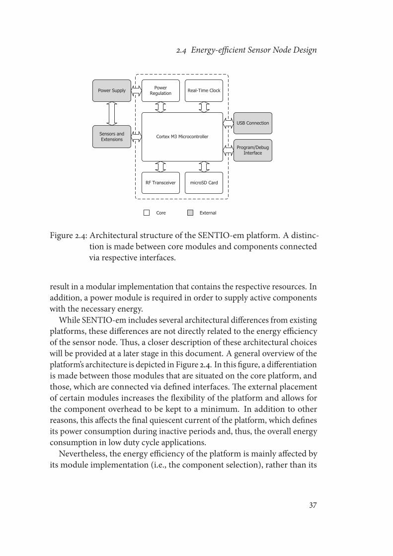
2.4 Energy-efficient Sensor Node Design
Cortex M3 Microcontroller
Real-Time Clock
RF Transceiver
Sensors and Extensions
Power Supply PowerRegulation
Program/Debug Interface
USB Connection
microSD Card
Core External
Figure 2.4: Architectural structure of the SENTIO-em platform. A distinc-tion is made between core modules and components connectedvia respective interfaces.
result in a modular implementation that contains the respective resources. Inaddition, a power module is required in order to supply active componentswith the necessary energy.
While SENTIO-em includes several architectural differences from existingplatforms, these differences are not directly related to the energy efficiencyof the sensor node. Thus, a closer description of these architectural choiceswill be provided at a later stage in this document. A general overview of theplatform’s architecture is depicted in Figure 2.4. In this figure, a differentiationis made between those modules that are situated on the core platform, andthose, which are connected via defined interfaces. The external placementof certain modules increases the flexibility of the platform and allows forthe component overhead to be kept to a minimum. In addition to otherreasons, this affects the final quiescent current of the platform, which definesits power consumption during inactive periods and, thus, the overall energyconsumption in low duty cycle applications.Nevertheless, the energy efficiency of the platform is mainly affected by
its module implementation (i.e., the component selection), rather than its
37
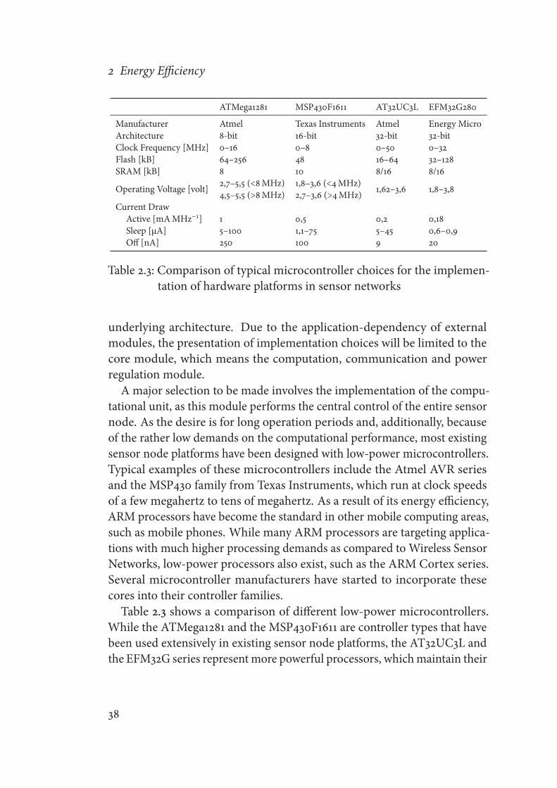
2 Energy Efficiency
ATMega1281 MSP430F1611 AT32UC3L EFM32G280
Manufacturer Atmel Texas Instruments Atmel Energy MicroArchitecture 8-bit 16-bit 32-bit 32-bitClock Frequency [MHz] 0–16 0–8 0–50 0–32Flash [kB] 64–256 48 16–64 32–128SRAM [kB] 8 10 8/16 8/16
Operating Voltage [volt] 2,7–5,5 (<8MHz) 1,8–3,6 (<4MHz) 1,62–3,6 1,8–3,84,5–5,5 (>8MHz) 2,7–3,6 (>4MHz)Current Draw
Active [mAMHz−1] 1 0,5 0,2 0,18Sleep [μA] 5–100 1,1–75 5–45 0,6–0,9Off [nA] 250 100 9 20
Table 2.3: Comparison of typical microcontroller choices for the implemen-tation of hardware platforms in sensor networks
underlying architecture. Due to the application-dependency of externalmodules, the presentation of implementation choices will be limited to thecore module, which means the computation, communication and powerregulation module.
A major selection to be made involves the implementation of the compu-tational unit, as this module performs the central control of the entire sensornode. As the desire is for long operation periods and, additionally, becauseof the rather low demands on the computational performance, most existingsensor node platforms have been designed with low-power microcontrollers.Typical examples of these microcontrollers include the Atmel AVR seriesand the MSP430 family from Texas Instruments, which run at clock speedsof a few megahertz to tens of megahertz. As a result of its energy efficiency,ARM processors have become the standard in other mobile computing areas,such as mobile phones. While many ARM processors are targeting applica-tions with much higher processing demands as compared to Wireless SensorNetworks, low-power processors also exist, such as the ARM Cortex series.Several microcontroller manufacturers have started to incorporate thesecores into their controller families.Table 2.3 shows a comparison of different low-power microcontrollers.
While the ATMega1281 and the MSP430F1611 are controller types that havebeen used extensively in existing sensor node platforms, the AT32UC3L andthe EFM32G series representmore powerful processors, whichmaintain their
38
2.4 Energy-efficient Sensor Node Design
focus on low-power consumption. As can be extracted from the propertylisting in the table, both of the more powerful processors outperform the pre-viously used controllers in most regards. The EFM32 controller, in particular,demonstrates the energy efficiency of its Cortex M3 core in both active andinactive states. As a result, this microcontroller allows for the desired tasksto be completed in a shorter period, leaving the controller running at lowerpower levels for a larger period of time.
Therefore, the EFM32G280 has been chosen as the core of the computationmodule on the SENTIO-em platform. It is driven by a 32MHz Q-MEMScrystal, which enables the platform to process data with a considerable speedimprovement as compared to traditional Micro Controller Unit (MCU) solu-tions, while maintaining similar power levels during processing due to itsimproved energy efficiency. In addition, the computational unit of SENTIO-em includes a Real-Time Clock (RTC) for accurate time-keeping, as well as amicroSD card slot for the storage of large amounts of sensor data. In bothcases, the energy efficiency of the final platform has driven the selectionprocess of the implementation. As SD cards have a considerable quiescentcurrent, the SD card interface contains an analog switch in its supply line,which allows for the interface to be completely cut from power, leaving onlythe leakage of the switch as the inactive consumption of this module. Such acreation of individual power domains, which can be controlled by the mi-crocontroller, is used more extensively with external platform modules and,thus, allows for the power consumption during inactive states to be kept at aminimum.The implementation choice of the communication module, on the other
hand, is rather more difficult. While the decision for the usage of an RFtransceiver is rather straightforward, different transceivers provide theirindividual properties, which makes it difficult to determine a clearly advan-tageous transceiver option. Table 2.4 contains several alternatives that havebeen considered for the implementation on SENTIO-em. The de-facto stan-dard in existing sensor nodes are transceivers with an integrated protocolin compliance with the IEEE 802.15.4 standard. Typical choices include theTexas Instruments CC2420 (and its successor, the CC2520), as well as Atmel’sRF23x series. Although these transceivers allow for a large set of existingcommunication protocols to be used, at times when these solutions are notrequired, the implemented protocol creates an undesired overhead. Further-
39

2 Energy Efficiency
CC1101 SX1233 CC2520 XBEE 802.15.4
Manufacturer Texas Instruments Semtech Texas Instruments Digi InternationalFrequency [MHz] 315/433/868/915 433/868/915 2400 2400Max. Data Rate [kbps] 500 600 250 250Sensitivity [dBm] -116 -120 -98 -100Output Power [dBm] -30 to +12 -18 to +17 -18 to +5 -10 to +18Current Draw
TX [mA] 12–34 16–95 25–37 45–250RX [mA] 14–17 16–17 18–25 50–55Sleep [μA] 0,2 0,1 <1 <10
Implemented Protocols none none low-level low / high-level
Table 2.4: Comparison of considered radio transceiver choices for the imple-mentation of SENTIO-em
more, the majority of these Integrated Circuits (ICs) operate in the 2.4GHzband, which limits their communication range considerably as compared tothose transceivers, which operate at lower frequencies [33].
As a result of their individual advantages and the application-dependencyof the desired transceiver properties, a flexible solution for the implementa-tion of the radio transceiver has been chosen. Physically, this implementationis oriented in accordance with the XBee communication module3, which hasgained tremendous attention, particularly, in the field of hobby electronics.Following the XBee’s footprint enables us to reuse existing transceiver mod-ule solutions, which range from simple IEEE 802.15.4 modules to high-power802.11 radios. At the same time, it becomes possible for personal implemen-tations of transceivers to be conducted in an easy manner. This allows for atransceiver with the best performance for a given application to be chosen,while limiting the overhead to a minimum.
Finally, while the interface for an external power supply circuit is provided,the core platform of SENTIO-em contains basic power regulation in order toguarantee the required levels for the components on board. This regulationhas been implemented based on a low-power Low Dropout (LDO) regulator,which only consumes quiescent currents of the order of 500 nA. Although theusage of a Switch Mode Power Supply (SMPS) leads to less losses as comparedto LDOs, these converters typically have higher quiescent currents, which
3http://www.digi.com/xbee/
40

2.4 Energy-efficient Sensor Node Design
results in an overall reduction in operational efficiency in low duty cycleapplications. As has been mentioned previously, additional power domainsare created for modules that have a considerable power consumption, evenduring inactivity. Utilizing analog switches or LDO regulators allows for thesemodules to be disabled with a minimal overhead in the system. Based on themodule that is switched off, however, increased start up times might be theconsequence, which has to be considered in each case.
2.4.2 SENTIO-em Evaluation
This section describes the evaluation of the SENTIO-em platform with re-spect to its energy efficiency and both methods for evaluating the energyefficiency and the obtained results will be presented.In order to evaluate the energy efficiency of the platform, both its power
consumption and computational performance have been measured. Fur-thermore, as the platform is intended for usage in applications within theenvironmental monitoring domain and, thus, will be deployed under varyingconditions, measurements have been conducted over a wide temperaturerange. Finally, the obtained measurement results are compared to the resultsobtained from existing sensor node implementations.
As SENTIO-em operates with a constant voltage, its power consumptioncan be measured by measuring the current consumption. For the measure-ment of platform currents, an Agilent 34410A4 digital multimeter has beenused. Furthermore, all results are based on a platform equipped with aSemtech SX1233 RF transceiver module. In order to create different environ-mental conditions, a measurement series has been conducted in an environ-mental test chamber5. While the platform will most likely not be exposed toall of these conditions, for the sake of completeness, the measurements havebeen conducted over the entire temperature range specified for the platform.Finally, the transition times between different operating states and timingsfor the evaluation of the processing performance have been measured with adigiview logic analyzer6.
4http://www.agilent.com5http://www.testequity.com/products/1104/6http://www.tech-tools.com/logic-analyzer.htm
41

2 Energy Efficiency
State Current Condition
Active 6.1mA 14MHz8mA 32MHz
Low-Power
2.3 μA EM11.6 μA EM21.2 μA EM31.8 μA EM3 + RTC
Radio 11–50 mA TX16.5mA RX
Table 2.5: Current consumption of SENTIO-em in its different operationstates. The measurements have been conducted under laboratoryconditions.
The results of the current consumption measurements, which were per-formed under laboratory conditions are listed in Table 2.5. These valuesrepresent the complete platform consumption. However, during Active andLow-Power state, the radio module has been set to sleep mode, whereasthe microcontroller has been in a low-power state (i.e., EM3) for the Radiomeasurements. The obtained values comply with the expectations based ondatasheet values. In the low-power mode EM3, for example, a platform cur-rent consumption of 1.2 μA has been measured, which matches the expectedvalues ideally (i.e., 600 nAMCU, 500 nA LDO, 100 nA radio). Figure 2.5 showsthe platform’s sleep mode consumption over its entire temperature range.While the current consumption remains low for all temperature values tested,a considerable increase in consumption can be detected at temperaturesabove 40 ○C. As opposed to the exponential leakage increase in low-powermodes, the active consumption increases linearly with temperature. An ex-ample is shown in Figure 2.6 for the transmission and reception current inthe radio transceiver. In comparison with the consumption increase duringinactivity, which in the worst condition can add up to 300% of its initialconsumption, the power consumption in active states only shows a smallpercentage increase.
In addition to the effect of low quiescent currents on the energy efficiencyof a sensor node, the active periodsmust be short. Thus, a sensor node should
42

2.4 Energy-efficient Sensor Node Design
−40 −20 0 20 40 60 80 1000
1
2
3
4
5
6
Temperature [degree C]
Cur
rent
Con
sum
ptio
n [u
A]
EM2EM3EM3+RTC
Figure 2.5: Temperature influence on the leakage currents of the SENTIO-em platform. Measurements have been conducted over the entirespecified temperature range for SENTIO-em. Humidity levelshave been constant at 40%.
−40 −20 0 20 40 60 8015
16
17
18
19
Temperature [deg C]
Cur
rent
Con
sum
ptio
n [m
A]
RXTX (0 dBm)
Figure 2.6: Temperature influence on the current consumption of SENTIO-em during communication tasks. Humidity levels have beenconstant at 40%.
be able to switch quickly between its different operation states, and performany given task in a rapid manner. Table 2.6 lists the transition times that havebeen measured for the SENTIO-em implementation. The obtained valuesshow that SENTIO-em is capable of fast transitions, taking less than 6 μs forthe processor to be operational and a few hundreds of μs until it becomesready to communicate7.
Figure 2.7 depicts the processing performance of the EFM32 controller onthe SENTIO-em platform in comparison to that for an Atmel ATMega1281,
7Using the Semtech SX1233 radio transceiver module
43

2 Energy Efficiency
From To Transition time
Sleep Active 1.8 – 5.8 μsRadio sleep TX 150 μsRadio sleep RX 380 μsTX RX 390 μsRX TX 70 μs
Table 2.6: Transition times between different operation states of the SENTIO-em platform. Transition times have been measured on a platformequipped with a Semtech SX1233 transceiver.
8−bit math 16−bit math 32−bit math float math 8−bit matrix 16−bit matrix matrix mul.0
100
200
300
400
Pro
cess
ing
time
[us]
FIR Whetstone0
5
10
15
Pro
cess
ing
time
[ms]
ATmega1281SENTIO−em
Figure 2.7: Evaluation of the processing performance of the SENTIO-emplatform in comparison with a typical microcontroller choice.Processing performance is measured by the processing time of aset of benchmarking functions.
which has previously been a highly popular choice for the implementationof sensor nodes. The computations performed are based on a benchmarkingsuite for microcontrollers8. This set of functions ranges from simple mathoperations, via matrix manipulations, to more complex operations, such asthe Whetstone benchmark. The figure contains the time periods taken bythe respective platform to perform the given task. While SENTIO-em hasbeen operating at a clock frequency of 32MHz, and thus four times fasterthan that of the ATMega1281 under test, its processing results show a timeimprovement of 6 to 46 times.
8http://www.ti.com/lit/an/slaa205c/slaa205c.pdf
44
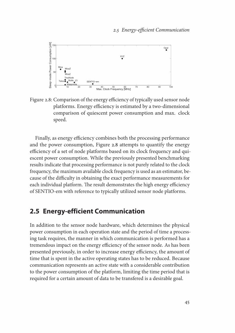
2.5 Energy-efficient Communication
0 10 20 30 40 50 60 70 80 90 1000
50
100
150
Max. Clock Frequency [MHz]Sle
ep−m
ode
Pow
er C
onsu
mpt
ion
[uW
]
MicaMicaZ
Mica2
TinyNodeTelos Mulle Z1
WaspmoteSENTIO−em
XYZ
Opal
Figure 2.8: Comparison of the energy efficiency of typically used sensor nodeplatforms. Energy efficiency is estimated by a two-dimensionalcomparison of quiescent power consumption and max. clockspeed.
Finally, as energy efficiency combines both the processing performanceand the power consumption, Figure 2.8 attempts to quantify the energyefficiency of a set of node platforms based on its clock frequency and qui-escent power consumption. While the previously presented benchmarkingresults indicate that processing performance is not purely related to the clockfrequency, the maximum available clock frequency is used as an estimator, be-cause of the difficulty in obtaining the exact performance measurements foreach individual platform. The result demonstrates the high energy efficiencyof SENTIO-em with reference to typically utilized sensor node platforms.
2.5 Energy-efficient Communication
In addition to the sensor node hardware, which determines the physicalpower consumption in each operation state and the period of time a process-ing task requires, the manner in which communication is performed has atremendous impact on the energy efficiency of the sensor node. As has beenpresented previously, in order to increase energy efficiency, the amount oftime that is spent in the active operating states has to be reduced. Becausecommunication represents an active state with a considerable contributionto the power consumption of the platform, limiting the time period that isrequired for a certain amount of data to be transfered is a desirable goal.
45
2 Energy Efficiency
A typical classification of communication methods in wireless commu-nications is the distinction between contention-based and contention-freeprotocols. Herein, contention-free protocols allow for certain communica-tion resources, such as time periods (Time DivisionMultiple Access (TDMA))or frequency channels (Frequency Division Multiple Access (FDMA)), to beallocated to individual nodes, whereas contention-based protocols create acompetitive environment for sensor nodes to perform their communicationtask. Based on its increased flexibility with respect to communication times,contention-based protocols, such as Carrier Sense Multiple Access (CSMA),have become the typical choice in wireless communication standards, suchas in IEEE 802.15.4 and IEEE 802.11. A common reason for this is that the un-scheduled manner of communication in these protocols allows for nodes tocompete for the channel at any point in time. As a result, the communicationlatencies are typically reduced and networks operating with a contention-based protocol support a higher degree of system dynamics, such as nodesjoining and leaving the network. Contention-free protocols, on the otherhand, provide a high reliability within static communication networks andoperate in an energy efficient manner.The energy efficiency of a communication protocol is defined by its ca-
pability to handle certain wasteful activities, such as those listed in Table2.7. As most of these parameters originate from unknown communicationtimes, they cannot be fully eliminated in contention-based communicationprotocols. Furthermore, functionalities provided in order to reduce suchactivities typically lead to an increase in protocol overhead. An example forthis is the implementation of Request-to-Send (RTS) and Clear-to-Send (CTS)control packets for the reduction of packet collisions, which, in turn, increasethe amount of data to be transmitted. Time scheduled protocols (i.e., TDMA),on the other hand, can significantly reduce (if not eliminate) the majorityof the named activities by the mere knowledge of the point in time duringwhich the communication will be conducted.
As the sensor nodes in the targeted application scenarios typically performa periodically occurring sampling task, TDMA-like communication protocolsbecome an ideal candidate for the energy efficient transport of measured datafrom the sensor node to the data collection point in the network. The typicalstructure of an TDMA protocol is depicted in Figure 2.9. In order to minimizethe effects of the parameters listed in Table 2.7, however, any uncertainties
46

2.5 Energy-efficient Communication
...Unallocated Time Slots
Allocated Time SlotsOverhead
TS1 TS2 TS3 ... TSn
Time frame
T1 T2 T3
t1 t2 t3 t4 tn tn+1
Figure 2.9: Overview on the typical structure of a TDMA communicationprotocol. Communication occurs within individual time slots.
regarding time must be retained at a minimum. Because of the resourcelimitations on typical sensor nodes, which prohibits the implementation oftiming circuits of high accuracy, there is a requirement for time synchroniza-tion between individual nodes to be performed. In the following sections,the difficulties of time synchronization in Wireless Sensor Networks will bepresented, and an energy efficient method for the implementation of timesynchronization for the purpose of communication will be presented.
2.5.1 Time Synchronization for Wireless Sensor Networks
There are several tasks in Wireless Sensor Networks, which demand or profitfrom a common notion of time between nodes. These include the time-stamping of samples, collaborative sampling of an event, and the measure-ment of time related properties (e.g., velocity). In order to achieve thiscommon notion of time, synchronization is mandatory. While synchroniza-tion requires communication and, thus, demands an increase in the spentenergy, synchronized communication can minimize unnecessary active pe-riods, which can lead to an overall more energy efficient communicationmethod.
The need for time synchronization between sensor nodes is based on non-ideal clock sources, implemented on these devices. Ideally, the time retainedby a sensor node C(t), should represent the reference time t, thus
C(t) = t . (2.12)
47

2 Energy Efficiency
Factor Description
Collision A collision is a superposition of two or more data transfers atthe same time. At the receiver this leads to a non-decomposablereception and therefore to data loss. In non-scheduled commu-nication collision is avoided by listen-before-sendmechanismsor additional control sequences, such as RTS and CTS packets.In scheduled protocols, this problem is solved by allocatingunique time periods for communication to nodes respectively.
Overhead Overhead is additional information that has to be sent withthe data, e.g. to determine source and destination. Overheadincreases in on-demand protocols when control sequencing isused. Depending on synchronization techniques, scheduledcommunication might also have increased overhead. In sched-uled communication, however, source identification might beomitted by using time allocation instead.
Over-Hearing Over-Hearing describes the problem of one node listening tocommunication, or part of the communication, dedicated to an-other node. While this problem is still applicable to on-demandprotocols, in scheduled communication each node is aware ofwhen data is meant to be targeted to itself and when not.
Over-Emitting Over-Emitting is the effect of one node transmitting data toanother node, while the receiver is not listening. The resultis similar to collisions, and once again it is solved by definingcommunication times in scheduled protocols.
Idle-Listening Idle-Listening occurs when the receiver is waiting for a trans-mission, listening to the channel without traffic occurring. Con-sumption in this state is similar to active reception. On-demandprotocols usually target this problem by listening periodicallyto the channel. Thus reducing, but not eliminating the im-pact. Scheduled communication ideally knows exactly whenthe transmission will start. However, in reality they are unableto eliminate idle-listening completely, because of the inaccuracyof the synchronization.
Table 2.7: Parasitic communication factors, that contribute to the energyconsumption of WSN nodes
48
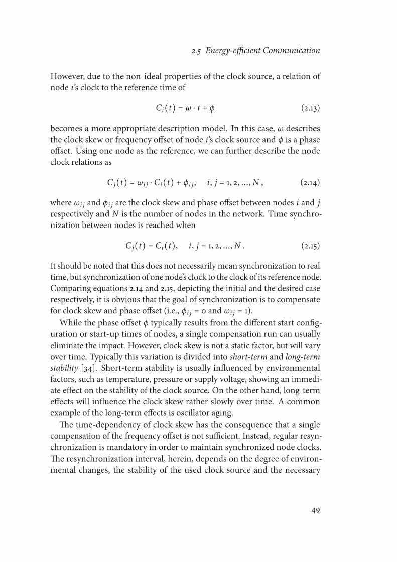
2.5 Energy-efficient Communication
However, due to the non-ideal properties of the clock source, a relation ofnode i’s clock to the reference time of
Ci(t) = ω ⋅ t + ϕ (2.13)
becomes a more appropriate description model. In this case, ω describesthe clock skew or frequency offset of node i’s clock source and ϕ is a phaseoffset. Using one node as the reference, we can further describe the nodeclock relations as
Cj(t) = ωi j ⋅ Ci(t) + ϕi j , i , j = 1, 2, ...,N , (2.14)
where ωi j and ϕi j are the clock skew and phase offset between nodes i and jrespectively and N is the number of nodes in the network. Time synchro-nization between nodes is reached when
Cj(t) = Ci(t), i , j = 1, 2, ...,N . (2.15)
It should be noted that this does not necessarily mean synchronization to realtime, but synchronization of one node’s clock to the clock of its reference node.Comparing equations 2.14 and 2.15, depicting the initial and the desired caserespectively, it is obvious that the goal of synchronization is to compensatefor clock skew and phase offset (i.e., ϕi j = 0 and ωi j = 1).While the phase offset ϕ typically results from the different start config-
uration or start-up times of nodes, a single compensation run can usuallyeliminate the impact. However, clock skew is not a static factor, but will varyover time. Typically this variation is divided into short-term and long-termstability [34]. Short-term stability is usually influenced by environmentalfactors, such as temperature, pressure or supply voltage, showing an immedi-ate effect on the stability of the clock source. On the other hand, long-termeffects will influence the clock skew rather slowly over time. A commonexample of the long-term effects is oscillator aging.The time-dependency of clock skew has the consequence that a single
compensation of the frequency offset is not sufficient. Instead, regular resyn-chronization is mandatory in order to maintain synchronized node clocks.The resynchronization interval, herein, depends on the degree of environ-mental changes, the stability of the used clock source and the necessary
49

2 Energy Efficiency
synchronization accuracy to be achieved in the respective applications.In general, ideal synchronization cannot be guaranteed, as the synchro-
nization method itself will introduce a certain amount of inaccuracy. Typicalways of establishing synchronization in WSNs, sources of inaccuracy, designconsideration and trade-off factors will be introduced in the following sec-tion.
Design Considerations and Sources of Inaccuracy
When implementing a synchronizationmethod for the creation of a commonnotion of time within the network, there are several design factors thatmust be considered. The majority of these factors are related and thereforelead to trade-off situations. These trade-offs have to be optimized for eachapplication or system case individually. Typical design considerations includesynchronization accuracy, the introduced energy cost of the synchronizationmethod, as well as its scalability and behavior in dynamic networks.Synchronization accuracy is the most obvious design factor, as synchro-
nization is implemented for a purpose, namely to create a common notionof time. However, a reduced synchronization accuracy might be acceptablewhen the remaining accuracy fulfills the requirements of the target applica-tion. Synchronization accuracy is related to allocated resources, thus alsoto energy cost. Additionally scalability might be limited when very highaccuracies are required to be reached. A major origin of inaccuracies is inrelation to delay components during wireless communication. An overviewof these delay components is given in Table 2.8 and their occurrence duringa packet transmission is presented in Figure 2.10.In energy constraint systems, such as Wireless Sensor Networks, the en-
ergy spent for synchronization can be a matter to be given consideration.Depending on the desired accuracy of the implementation, considerableamounts of energy can be spent in the communication or processing stages.In particular, when synchronization is used to reduce energy consumption,such as its utilization for accurate TDMA schedules, limiting the energy over-head spent by the synchronization approach is of major importance. Usuallyenergy cost considerations conflict with synchronization accuracy and mightinfluence the reliability of the network in dynamic situations.Scalability and dynamic network behavior are factors that should be con-
50

2.5 Energy-efficient Communication
sidered in any sensor network, which is planned to be deployed. Scalabilityherein describes how the synchronization accuracy is influenced with theincreasing size of the network. A typical problem is in relation to addi-tional delays due to multi-hop synchronization. On the other hand, dynamicnetwork behavior deals with situations, such as the packet loss during the(re-)synchronization process.
Time SynchronizationMethods and Classification
In essence, time synchronization between sensor nodes is established byreporting one node’s time to the other node(s). As introduced in Table 2.8, the
Delay Component Description
Send Time Time period of handling the send request and prepar-ing the packet transmission. Influenced by system loadand overhead. Can be reduced by limiting system loadby predicting time of resynchronization.
Access Time Time of accessing the transmission medium. Influ-enced by network load. Usually high in contention-based protocols, while low for scheduled communica-tion.
Transmission Time Time to actually transmit the packet to the medium.Depends on the packet size, but can be estimated ratheraccurately.
Propagation Time Time the message needs to propagate from sender toreceiver. Depends on the distance between the twonodes. Comparably small in typical RF-based and short-range WSNs.
Reception Time Time it takes to receive the packet at the receiver’s side.Complementary to Transmission Time.
Receive Time Time for processing the received packet until the appli-cation is informed. Complementary to Send Time.
Table 2.8: Delay factors in Wireless Sensor Network transmissions, influenc-ing synchronization accuracy when not addressed
51

2 Energy Efficiency
Send Access Transmission
Reception Receive
Time t
Propagation
Communication intention
Reception information
Figure 2.10: Occurrence of delay components during a packet transmissionbetween two nodes in a Wireless Sensor Network
transmission of packets occurs with a mainly unpredictable delay, reportinga timestamp of the past at the receiver when used for synchronization. Thisprinciple is illustrated in Figure 2.11a and can be formally described by
CB(t2) = CA(t1) + ϕAB + δ , (2.16)
wherein ϕAB is the clock offset between node A and B, and δ describesthe sum of the delay components. Being interested in determining ϕAB,δ acts as a parasitic effect on the synchronization. In order to reduce itsinfluence, the delay components in the system can be minimized, or theycan be estimated/measured for compensation purposes.A typical way of dealing with the latter case, is by using bidirectional
communication in order to implement synchronization. This enables theestimation of the delay components from the measurement of round-tripdelays. This method can be graphically demonstrated as shown in Figure2.11b. Formally, it is possible to add the backward transmission
CA(t4) = CB(t3) + ϕBA + δ, ϕBA = −ϕAB (2.17)
to the description, and thus be able to estimate both, δ and ϕAB as
δ = (CB(t2) − CA(t1)) + (CA(t4) − CB(t3))2
(2.18)
52
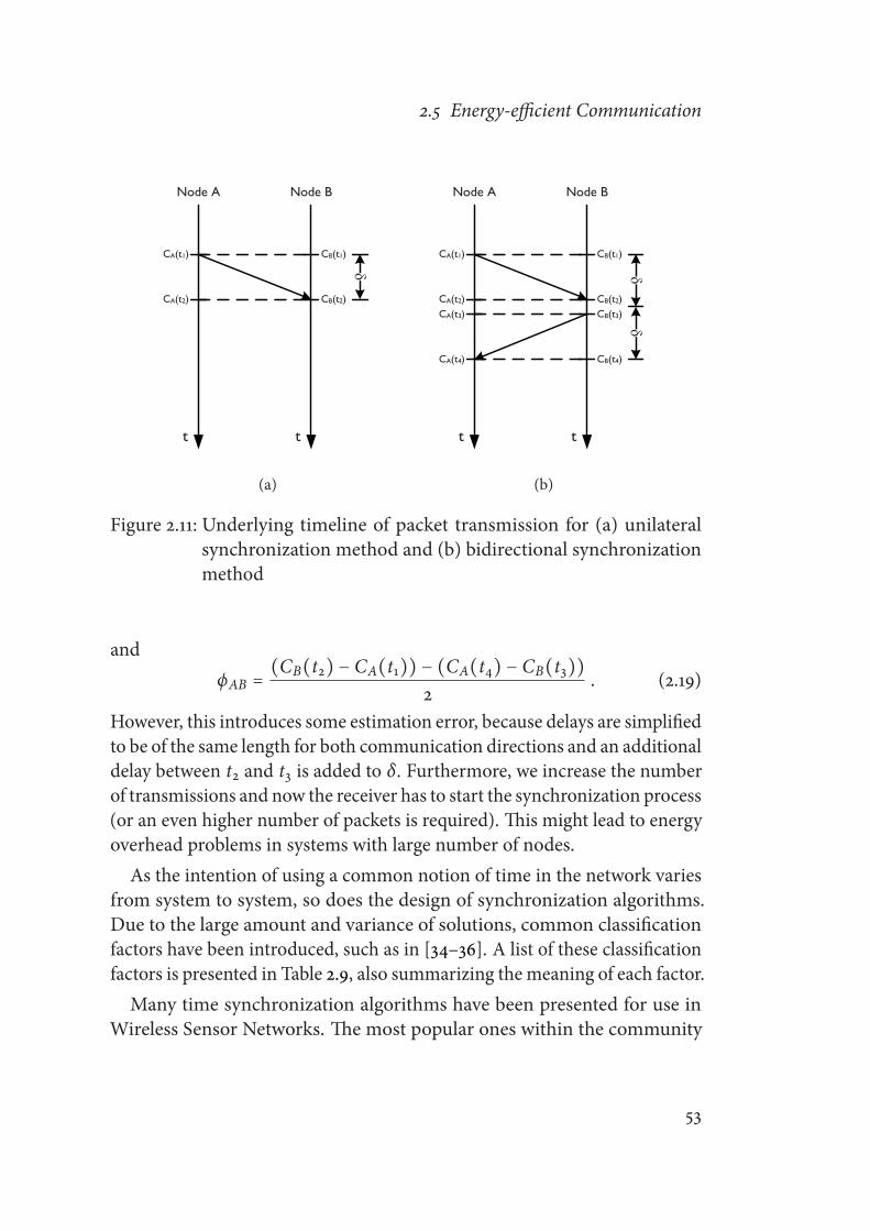
2.5 Energy-efficient Communication
t t
Node A Node B
�
CA(t1)
CA(t2)
CB(t1)
CB(t2)
(a)
t t
Node A Node B
�CA(t1)
CA(t2)
CB(t1)
CB(t2)CB(t3)
CB(t4)
CA(t3)
CA(t4)
�
(b)
Figure 2.11: Underlying timeline of packet transmission for (a) unilateralsynchronization method and (b) bidirectional synchronizationmethod
andϕAB = (CB(t2) − CA(t1)) − (CA(t4) − CB(t3))
2. (2.19)
However, this introduces some estimation error, because delays are simplifiedto be of the same length for both communication directions and an additionaldelay between t2 and t3 is added to δ. Furthermore, we increase the numberof transmissions and now the receiver has to start the synchronization process(or an even higher number of packets is required). This might lead to energyoverhead problems in systems with large number of nodes.
As the intention of using a common notion of time in the network variesfrom system to system, so does the design of synchronization algorithms.Due to the large amount and variance of solutions, common classificationfactors have been introduced, such as in [34–36]. A list of these classificationfactors is presented in Table 2.9, also summarizing the meaning of each factor.Many time synchronization algorithms have been presented for use in
Wireless Sensor Networks. The most popular ones within the community
53

2 Energy Efficiency
of WSNs, are Timing-Sync Protocol for Sensor Networks (TPSN) [37], Refer-ence Broadcast Synchronization (RBS) [38], Flooding Time SynchronizationProtocol (FTSP) [39], Lightweight Time Synchronization (LTS) [40], PairwiseBroadcast Synchronization (PBS) [41] and TimeDiffusion Protocol (TDP) [42].Because of their intended use in WSN applications, energy efficiency is ad-dressed in all of them. Nonetheless, as most of these synchronization mecha-nism are based on the bidirectional synchronization method, the numberof packet transmissions in order to establish synchronization can be ratherhigh. However, FTSP is based on the unilateral approach and therefore limitsthe number of packet transmissions. To address delay components, however,low level time-stamping is used and several packets are sent to allow for theestimation of clock-skew via linear regression.
When time synchronization has its main purpose in energy savings, suchas in the case targeted here, the number of communication packets usedfor establishing a common notion of time, which essentially describe theenergy overhead for the synchronization algorithm, becomes one of themajorconcerns. However, at the same time the protocol has to maintain a certaindegree of accuracy, allowing for energy-efficient, but stable communication.
2.5.2 Synchronized Duty-Cycling
As mentioned previously, typical sampling intervals in environmental moni-toring WSNs are of the order of minutes. This is due to the measurement oftypically slowly changing parameters, such as temperatures, humidities orgas concentrations. In networks with a large number of sensor nodes, thismeans that new data is sampled at a rather slow rate, but once sampling isdue, a large number of nodes want to communicate their data to a centralcollection point. The lack of synchronization in this situations has a twofoldimpact. On the one hand, sampling should usually occur at the same timeat all nodes in order to obtain comparable sensor samples. Lacking timesynchronization in this case means that data correlation cannot be guaran-teed. On the other hand, the transmission of the sampled data has to becoordinated. In a common on-demand protocol the nodes would attempt totransmit their data directly after sampling, which might lead to packet colli-sions. Using a scheduled transmission method without a common timebaseonly partially solves this issue, as different node clock skews can result in
54

2.5 Energy-efficient Communication
overlapping transmission periods.A synchronization algorithm, targeting these issues in the present appli-
cation, should have certain properties. Synchronization should be network-wide, as all end-nodes are involved in the communication process. Thesynchronization should allow communication at any time, thus an algorithmthat maintains synchronization of the nodes is preferable over on-demandsynchronizing solutions. Resulting accuracy is not the main target of theprotocol, but the best achievable accuracy, in order to minimize the en-ergy requirements, is desired. As energy overhead is the main concern, theoptimization goal for the solution is minimum energy, thus minimum com-munication overhead.A major consequence of the limited communication to be performed, is
that all pairwise synchronization schemes are inappropriate. Consideringthe goal of minimizing communication, a single synchronization message isthe desired outcome. Using the broadcast capability of the RF-channel, thesame message can be used to synchronize all nodes in the same broadcast
Classification Factor Description
Internal/External Describes whether the algorithm synchronizes net-work nodes to some sort of external clock sourceor only amongst each other
Always/On-demand Describes whether nodes stay synchronized all thetime or whether they are synchronized on-demand
All/Subset Describes whether all nodes will be synchronizedor only a subset of nodes
Rate/Offset Describes whether nodes synchronize to the sameclock rate or whether a clock offset is compensatedfor
Correction/Translation Describes whether node clocks are corrected to thecommon time or whether the timescale is trans-lated
Table 2.9: Main classification factors of time synchronization algorithms inWireless Sensor Networks
55

2 Energy Efficiency
t1 t2 t3
t1 t3t1' t2 t2' t3'
t
CA(T12)
CB(T1'2')
Node A
Node B
Figure 2.12: Timeline of an interval-measurement based synchronizationmethod
domain. A single (unidirectional) synchronization message, does, to someextent, enable for the compensation of the phase offset between nodes, butit does not address the clock skew. However, as periodic resynchronizationis required to address temporary changes, frequency information can beextracted from the time interval between two synchronization broadcasts.As depicted in Figure 2.12, in an interval-based synchronization method,
message transfer occurs periodically and unidirectionally. The node act-ing as the clock reference periodically broadcasts a synchronization packet,which can be interpreted as a typical Start Frame Delimiter (SFD) for thesynchronization frame. Theoretically, there is no content necessary withinthis message, but, as the packet has to be transfered anyway, some globalinformation might as well be included. If indeterministic delay components,such as access time or system load, are handled to be minimal, the transmis-sion delay of the two following packets can be estimated as a constant value.Therefore, as indicated in Figure 2.12, we can define
δ = t′1 − t1 = t′2 − t2 = t′i − ti . (2.20)
This means, a synchronization message sent by node A at ti will arrive anunknown time later at node B at the time t′i , with
t′i = ti + δ . (2.21)
Furthermore, when defining a constant interval T between synchronizationmessages, node A will periodically send out synchronization messages with
56

2.5 Energy-efficient Communication
its own understanding of periodicity T , namely
CA(T) = CA(ti+1) − CA(ti) . (2.22)
Allowing node B to measure the interval between two consecutive synchro-nization messages will lead to a measured inter-packet length of
CB(CA(T)) = CB(t′i+1) − CB(t′i) . (2.23)
As the delay components of both transmissions are estimated as being con-stant, the real-time length of both intervals will be the same, thus
C(CA(T)) = C(CB(CA(T))) , (2.24)
withC(T) = T . (2.25)
At this point, all receiver nodes only know their interpretation of the refer-ence interval CA(T) and the ideal synchronization interval T . They do notknow the real synchronization interval itself. However, as for communicationpurposes, internal synchronization is usually sufficient and the nodes cantreat the measured interval as the ideal interval. This leads to the fact thatthe nodes do not synchronize to real time C(t), but to the reference’s inter-pretation of the real time CA(t). For the previous example, we can thereforeredefine node B’s point of view as
CB(CA(T)) ∶= CB(T) . (2.26)
This will be false in the majority of cases and only holds true if
CA(T) = C(T) . (2.27)
However, for the purpose of internal synchronization, the redefinition doesnot introduce any error, as long as node A is defined as holding the referenceclock.
Knowing both, T and CB(T), node B can simply calculate its difference
57

2 Energy Efficiency
from the reference clock
D(T) = T − CB(T) , (2.28)
wherein a positive D(T) denotes a slow clock compared to the reference anda negative D(T) a fast clock. Furthermore, by knowing the time intervalT over which this clock difference occurred, node B has the possibility toestimate its drift rate relative to the reference node and thereby translate anypoint in time to its own timebase, using
CB(t) = t − D(T) ⋅ tT
. (2.29)
This translation is useful, when it comes to communication schedules, as thesynchronization reference, which should be the clusterhead of a communica-tion cluster, can schedule communication in terms of its own timebase. Allnodes willing to communicate will then translate their allocated communi-cation times to their local timebase. Hence, all nodes will communicate ina schedule, based on the reference timebase, avoiding overlapping commu-nications (i.e., collisions). Additionally, local measurement of the referencesynchronization period allows for unused time being spent in low-powermode, while waking up in a precise manner for the reception of the nextsynchronization message (i.e., the start of a new communication frame) orany other activity scheduled to be performed. A general time-line of thesynchronization procedure is given in Figure 2.13. This provides a closer lookat what happens each time a synchronization message is sent in Figure 2.12.
With ideal synchronization, waiting for the synchronization packet recep-tion (colored in Figure 2.13) would not be necessary. However, because thereare variations in local clock frequencies due to environmental parameters,quantization errors in reading and setting timer events, as well as variationsin component wakeup times, a certain guard-time is desired. This guard-time should guarantee that the node is in a state allowing the reception ofthe synchronization message, once it occurs. Nonetheless, at the same timethe guard-time should be as short as possible, while fulfilling the previouslymentioned task.An important measure to define the length of the guard-time is the accu-
racy of the wake-up time. This value is based on, but is not limited to, the
58
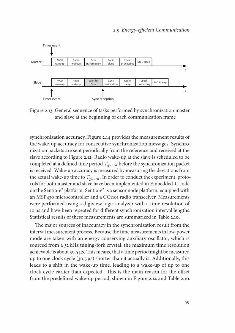
2.5 Energy-efficient Communication
t
MCU wakeup
Timer event
Radio wakeup
Wait for Sync
Sync verification
Sync reception
Local processing
Radio sleep MCU sleepSlave
t
MCU wakeup
Timer event
Radio wakeup
Sync transmission
Local processing
Radio sleep MCU sleepMaster
Figure 2.13: General sequence of tasks performed by synchronization masterand slave at the beginning of each communication frame
synchronization accuracy. Figure 2.14 provides the measurement results ofthe wake-up accuracy for consecutive synchronization messages. Synchro-nization packets are sent periodically from the reference and received at theslave according to Figure 2.12. Radio wake-up at the slave is scheduled to becompleted at a defined time period Tguard before the synchronization packetis received. Wake-up accuracy is measured by measuring the deviations fromthe actual wake-up time to Tguard . In order to conduct the experiment, proto-cols for both master and slave have been implemented in Embedded-C codeon the Sentio-e2 platform. Sentio-e2 is a sensor node platform, equipped withan MSP430 microcontroller and a CC1101 radio transceiver. Measurementswere performed using a digiview logic analyzer with a time resolution of10 ns and have been repeated for different synchronization interval lengths.Statistical results of these measurements are summarized in Table 2.10.The major sources of inaccuracy in the synchronization result from the
interval measurement process. Because the timemeasurements in low-powermode are taken with an energy conserving auxiliary oscillator, which issourced from a 32 kHz tuning-fork crystal, the maximum time resolutionachievable is about 30.5 μs. Thismeans, that a time periodmight bemeasuredup to one clock cycle (30.5 μs) shorter than it actually is. Additionally, thisleads to a shift in the wake-up time, leading to a wake-up of up to oneclock cycle earlier than expected. This is the main reason for the offsetfrom the predefined wake-up period, shown in Figure 2.14 and Table 2.10.
59
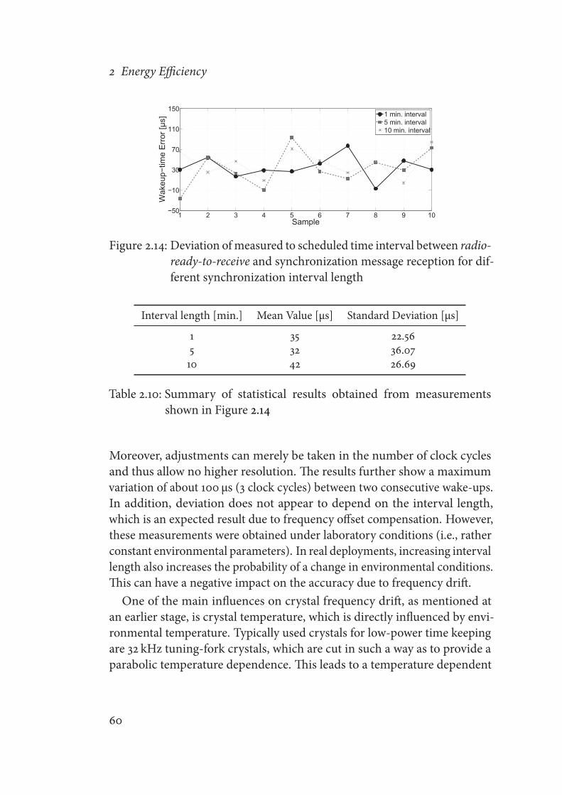
2 Energy Efficiency
1 2 3 4 5 6 7 8 9 10−50
−10
30
70
110
150
Sample
Wak
eup−
time
Err
or [μ
s]
1 min. interval5 min. interval10 min. interval
Figure 2.14: Deviation ofmeasured to scheduled time interval between radio-ready-to-receive and synchronization message reception for dif-ferent synchronization interval length
Interval length [min.] Mean Value [μs] Standard Deviation [μs]
1 35 22.565 32 36.0710 42 26.69
Table 2.10: Summary of statistical results obtained from measurementsshown in Figure 2.14
Moreover, adjustments can merely be taken in the number of clock cyclesand thus allow no higher resolution. The results further show a maximumvariation of about 100 μs (3 clock cycles) between two consecutive wake-ups.In addition, deviation does not appear to depend on the interval length,which is an expected result due to frequency offset compensation. However,these measurements were obtained under laboratory conditions (i.e., ratherconstant environmental parameters). In real deployments, increasing intervallength also increases the probability of a change in environmental conditions.This can have a negative impact on the accuracy due to frequency drift.One of the main influences on crystal frequency drift, as mentioned at
an earlier stage, is crystal temperature, which is directly influenced by envi-ronmental temperature. Typically used crystals for low-power time keepingare 32 kHz tuning-fork crystals, which are cut in such a way as to provide aparabolic temperature dependence. This leads to a temperature dependent
60
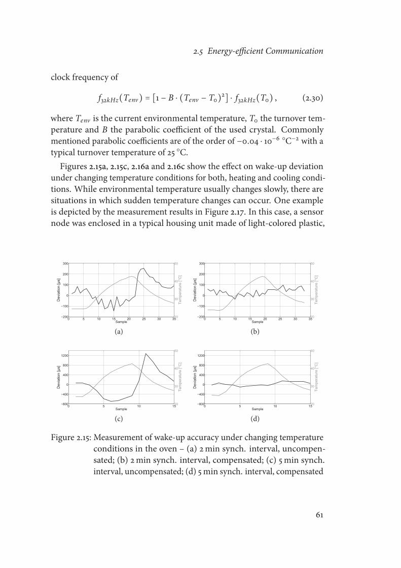
2.5 Energy-efficient Communication
clock frequency of
f32kHz(Tenv) = [1 − B ⋅ (Tenv − T0)2] ⋅ f32kHz(T0) , (2.30)
where Tenv is the current environmental temperature, T0 the turnover tem-perature and B the parabolic coefficient of the used crystal. Commonlymentioned parabolic coefficients are of the order of −0.04 ⋅ 10−6 ○C−2 with atypical turnover temperature of 25 ○C.Figures 2.15a, 2.15c, 2.16a and 2.16c show the effect on wake-up deviation
under changing temperature conditions for both, heating and cooling condi-tions. While environmental temperature usually changes slowly, there aresituations in which sudden temperature changes can occur. One exampleis depicted by the measurement results in Figure 2.17. In this case, a sensornode was enclosed in a typical housing unit made of light-colored plastic,
0 5 10 15 20 25 30 35−200
−100
0
100
200
300
Sample
Dev
iatio
n [μ
s]
20
30
40
50
Tem
pera
ture
[°C
]
(a)
0 5 10 15 20 25 30 35−200
−100
0
100
200
300
Sample
Dev
iatio
n [μ
s]
20
30
40
50
Tem
pera
ture
[°C
]
(b)
0 5 10 15−800
−400
0
400
800
1200
Sample
Dev
iatio
n [μ
s]
20
30
40
50
Tem
pera
ture
[°C
]
(c)
0 5 10 15−800
−400
0
400
800
1200
Sample
Dev
iatio
n [μ
s]
20
30
40
50
Tem
pera
ture
[°C
]
(d)
Figure 2.15: Measurement of wake-up accuracy under changing temperatureconditions in the oven – (a) 2min synch. interval, uncompen-sated; (b) 2min synch. interval, compensated; (c) 5min synch.interval, uncompensated; (d) 5min synch. interval, compensated
61

2 Energy Efficiency
0 5 10 15 20 25 30−50
50
150
250
350
450
550
Sample
Dev
iatio
n [μ
s]
−20
−10
0
10
20
Tem
pera
ture
[°C
]
(a)
0 5 10 15 20 25−50
50
150
250
350
450
550
Sample
Dev
iatio
n [μ
s]
−20
−10
0
10
20
Tem
pera
ture
[°C
]
(b)
1 2 3 4 5 6 7 8 9 10 11−400
0
400
800
1200
1600
2000
2400
Sample
Dev
iatio
n [μ
s]
−10
0
10
20
30
Tem
pera
ture
[°C
]
(c)
0 2 4 6 8 10 12−400
0
400
800
1200
1600
2000
2400
Sample
Dev
iatio
n [μ
s]−10
0
10
20
30
Tem
pera
ture
[°C
]
(d)
Figure 2.16: Measurement of wake-up accuracy under changing temperatureconditions after cooling in the freezer – (a) 2min synch. interval,uncompensated; (b) 2min synch. interval, compensated; (c)5min synch. interval, uncompensated; (d) 5min synch. interval,compensated
then placed in direct sunlight. Similar situations might occur when a nodewas situated in the shade for a while, before being exposed to direct sunlight.The temperature inside the box was logged using an on-board temperaturesensor with a rate of 1Hz over a period of 40min. It can be seen, that a rapidtemperature change in the first minutes after exposure can be expected.
Knowledge of the temperature of the clock crystal enables compensation tobe made for the drift occurring due to deviation from turnover temperature.Implementing a low-power temperature sensor on the sensor node is inex-pensive and is often required for calibration or application purposes. Whenused for temperature drift compensation, however, close spatial location tothe crystal should be ensured in order to achieve as accurate readings ofcrystal temperature as possible.An initial measurement of clock drift over increasing temperature for
62
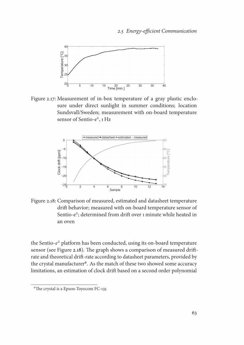
2.5 Energy-efficient Communication
0 5 10 15 20 25 30 35 4020
25
30
35
40
Time [min.]
Tem
pera
ture
[°C
]
Figure 2.17: Measurement of in-box temperature of a gray plastic enclo-sure under direct sunlight in summer conditions; locationSundsvall/Sweden; measurement with on-board temperaturesensor of Sentio-e2, 1 Hz
0 2 4 6 8 10 12 14−25
−20
−15
−10
−5
0
Sample
Clo
ck d
rift [
ppm
]
25
30
35
40
45
50
Tem
pera
ture
[°C
]
measured datasheet estimated measured
Figure 2.18: Comparison of measured, estimated and datasheet temperaturedrift behavior; measured with on-board temperature sensor ofSentio-e2; determined from drift over 1minute while heated inan oven
the Sentio-e2 platform has been conducted, using its on-board temperaturesensor (see Figure 2.18). The graph shows a comparison of measured drift-rate and theoretical drift-rate according to datasheet parameters, provided bythe crystal manufacturer9. As the match of these two showed some accuracylimitations, an estimation of clock drift based on a second order polynomial
9The crystal is a Epson-Toyocom FC-135
63

2 Energy Efficiency
has been added. The estimation is obtained in the form of
Δest(Tenv) = a ⋅ (Tenv − T0)2 + b ⋅ (Tenv − T0) + c , (2.31)
where Δest is the estimated drift and a, b, c are the calibration parameters.The results show, that if high accuracy is required, an initial calibration runcan provide accuracy within 1 ppm. However, in the case where the calibra-tion is too time and cost expensive, datasheet values can be used to predictoccurring clock drift with restricted accuracies. For measurements shownin Figures 2.15 and 2.16, a calibrated temperature compensation method hasbeen implemented. Comparing these results with those for uncompensatedresults, illustrates that temperature dependent clock drift can be almost com-pletely eliminated by using a temperature compensation technique based oncrystal temperature measurement.Nonetheless, measuring the crystal temperature adds additional costs to
the synchronization algorithm. Sampling the temperature sensor periodicallyduring the inactive period requires the processor to wake-up and read thecurrent temperature value. Furthermore, additional active time is mandatoryto process the taken values and calculate the expected drift according toequation 2.31. This has to be accomplished once the last temperature readinghas been sampled and before the radio wake-up should occur, allowing foran adjustment of the scheduled wake-up time. These necessary activitieswill increase the microcontroller duty cycle and therefore lower the energy-efficiency. On the other hand, temperature drift can also be handled byapplying longer guard-times, while not compensating for changing temper-ature. While this consumes no sampling related energy, the radio modulehas to be in the reception state for a longer time, thus spending more energy.As temperature drift has to be dealt with, the question remains which of themethods is the more energy-efficient.
Estimating additional energy costs by adding expected power consumptionlevels and periods for each of the methods can provide the answer. This leadsto
PtmpComp = Tmeas ⋅ Nmeas ⋅ PmeasTf rame
+ Tprocess ⋅ Pprocess (2.32)
for a temperature compensating approach. In this case, Tmeas is the timeperiod for taking a sample from the temperature sensor,Nmeas are the number
64

2.5 Energy-efficient Communication
Parameter Value Description
Tmeas 950 μs Time for measurement of a temperature sampleTf rame 60 s to 600 s Time of the synchronization intervalTprocess 150 μs Time for processing the temperature driftTsync 2ms Time for receiving the sync packetPmeas 2mA Consumption during temperature samplingPprocess 2mA Consumption during processingPRX 20mA Consumption when radio in reception state
Table 2.11: Parameter overview for estimations in Figure 2.19, obtained frommeasurements on Sentio-e2
of temperature samples in one synchronization frame, Pmeas the consumptionlevel during a sample, Tf rame the time of a synchronization frame, whileTprocess and Pprocess are the time and power consumption of processing thetemperature drift respectively.
Likewise, the consumption for providing an additional guard-period canbe summed up as
Pguard = Δ(θdi f ,max) ⋅ Tf rame ⋅ PRX , (2.33)
with PRX being the power consumption level in reception state, Tf rame thesynchronization period as above, and Δ(θdi f ,max) the drift rate, determinedby the maximum temperature difference from the turnover temperature.An estimation was conducted with parameters, measured on Sentio-e2,
which are listed in Table 2.11. The respective results obtained are shown inFigure 2.19. In addition to the compensation cost, the energy demands for thereception of the synchronization message have been included, which resultsin the complete energy cost of the temperature-robust synchronization algo-rithm to be provided. The calculations show that temperature compensationis the more energy-efficient solution in almost all cases. Providing enlargedguard-periods is only recommended if, during the whole deployment time,no large temperature variations are expected.
Finally, integrated RTC circuits become an essential part in many productsand offer ever increasing functionality. As has been presented in Section2.4, our current node platform uses such an RTC, which operates with a
65

2 Energy Efficiency
1 2 3 4 5 6 7 8 9 100
1
2
3
4
5
Pow
er C
onsu
mpt
ion
[�W
]
Sync Interval [min]
Sampling interval: 5 sec.Sampling interval: 10 sec.Sampling interval: 15 sec.Sampling interval: 30 sec.
(a)
1 2 3 4 5 6 7 8 9 100
1
2
3
4
5
Pow
er C
onsu
mpt
ion
[�W
]
Sync Interval [min]
Temperature difference: 45°Temperature difference: 35°Temperature difference: 25°Temperature difference: 15°
(b)
Figure 2.19: Comparison of power consumption needed to deal with tem-perature drift – (a) Temperature compensation with differenttemperature sampling rates; (b) Extending reception guard-timefor differentmaximumdeviations from the turnover temperature
temperature-compensated internal quartz crystal. While the synchronizationmethod, which has been presented here, was also implemented on SENTIO-em, a comparison of the cost-performance ratio with respect to software andhardware based temperature compensation is yet to be made.
66

3 Solar Energy Harvesting
While the focus of the previous chapter lay on the increase of energy efficiencyin order to prolong the sensor node lifetime, in this chapter solar energyharvesting will be addressed as a method to increase the energy supply towireless sensor nodes and, thus, prolong their lifetime.
After providing the motivation for the usage of energy harvesting in gen-eral, and solar energy harvesting in particular, as the power supply for wirelesssensor nodes in the environmental monitoring domain, solar energy har-vesting will be addressed threefold. Firstly, we will address solar energyharvesting architectures, wherein the focus lies on long system lifetime andlow irradiance conditions. Secondly, we will address solar energy harvest-ing simulations with a focus on architecture dimensioning. Finally, we willpresent the method and implementation of a solar energy harvesting testbedin order to simplify architectural evaluations and provide systematic compar-ison possibilities.
3.1 Solar Energy Harvesting
Although sensor nodes in Wireless Sensor Networks can typically be con-sidered as low-power devices and therefore consume rather small currentsover time, any energy source with finite capacity (e.g., batteries) will provideenergy for only a limited amount of time. As was mentioned previously, thiscontradicts the desire for autonomous measurement systems to operate in aperpetual manner.Figure 3.1 shows a simplified analysis of battery lifetime for varying load
currents. Simplification is made in several ways, namely, the nominal batterycapacity (in this case 2000mAh) is assumed to be the real capacity, that theenvironment will not degrade capacity, no self-discharge is included and noenergy is spent for voltage conversion inefficiencies (here assumed from 1.5 V
67

3 Solar Energy Harvesting
0 0,1 0,2 0,3 0,4 0,50
2
4
6
8
10
12
Average Current Consumption [mA]
Sup
ply
Tim
e [y
ears
]
Figure 3.1: Simplified energy supply time from an AA-type battery in idealsituations
to 3V). Hence, the illustrated case thus presents a very optimistic lifetimeand a lower lifetime should be expected in reality.Nevertheless, this qualitative description illustrates, that the lifetime for
sensor nodes, powered by batteries, can be very limited and decreases dra-matically with increasing consumption. One possible solution is to increasethe number of batteries and thus accumulate capacity. However, this onlypartially solves the problem, as the available capacity will remain limited.In addition, this solution introduces some undesirable drawbacks. Theseinclude the linearly increasing size and cost of the system caused by theincreasing number of batteries. Additionally, there is an increasing strainplaced on the environment, especially if systems are deployed in locationswhere it is impossible to recover the system. Alternatively, rechargeable bat-teries can be implemented, thus reducing the number of battery exchanges.However, recharging still demands a considerable amount of manpower andis not usually a feasible option in the field and the usable capacity is reduceddue to the greatly increased self-discharge rates, whichmay be as high as 10%to 20% per year [43]. Moreover, rechargeable batteries display a more rapideffect of degradation, due to the chemical process, which occurs during thecharge and discharge at the electrodes. This leads to a reduced componentlifetime for these batteries, typically of the order of a few years for commonlyused technologies.
A desirable solution, in these scenarios, is to use an energy storage devicewith limited capacity, that can be autonomously recharged by using ambientenergy sources. As ambient sources, such as wind or sun, can be classified
68

3.1 Solar Energy Harvesting
Energy Source Power Density Condition
Solar 100mWcm−2 Direct sunlight, outdoorsWind 100mWcm−2 9m s−1 wind speed, 10m altitudeAmbient RF < 1 μWcm−2 Not close to emission sourceThermo-Electric 60 μWcm−2 5 ○C temperature difference
Table 3.1: Typical energy harvesting sources and their power levels availablein outdoor environments; based on [30, 44]
as inexhaustible energy sources – meaning that they have no capacity limit– it becomes possible to perpetually replenish a used storage device withlimited capacity. From the load perspective, an unlimited energy supplyhas thus been attached. Nevertheless, for this to operate successfully, theconversion rate, consumption rate, storage capacity and storage lifetime haveto be properties which are all matched. This means that, while the energycan be perpetually supplied from the ambient sources, this supply is limitedto certain rates. Thus, as opposed to the capacity-limited energy sourcethat batteries do represent, energy harvesting can typically be classified asrate-limited.
Table 3.1 provides an overview of ambient energy sources, commonly usedin energy harvesting with their respective power densities. While conversionfrom solar and wind both provide sufficient power densities, solar energy con-version possesses some advantages over wind. Although both technologiescan be considered as relatively mature conversion techniques, solar energyconversion is additionally readily scalable in size. Furthermore, solar energyinvolves no mechanical parts, which are exposed to limited component life-time and/or require maintenance. Solar energy harvesting, thus, has been apopular choice in Wireless Sensor Networks that are deployed in outdoorenvironments, such as is typical in the environmental monitoring domain.
3.1.1 Energy Neutral Operation
Although solar energy harvesting can provide high power levels as comparedto other ambient energy sources, it is not only rate-limited, but its rate istemporally and spatially dependent. Despite these variations in supply levels
69

3 Solar Energy Harvesting
that can be harvested, it is desirable to have an uninterrupted supply of theattached system (i.e., the sensor nodes). Therefore, the load power consump-tion has to match the power supply rate of the harvesting system. A metric,called the energy neutral operation [45], can be used in order to describe therelationship between consumption and supply, providing energy to the loadat all times. Discussions concerning an energy neutral operation, however,only make sense in connection with energy sources of infinite energy supplycapability, while being restricted by certain supply rates. This, for example,means that it is not possible for a primary battery to operate in an energyneutral manner, because its energy reservoir is finite.
The simplest form of an energy neutral operation is the direct connectionof the energy harvesting source to the load. In this case, the supplied powerhas to exceed the consumed power at any time, such as
Ps(t) ≥ Pc(t) , (3.1)
with Ps(t) being the supplied power and Pc(t) the consumed power at timet respectively. However, in this scenario all the energy of times Ps(t) > Pc(t)and Ps(t) < Pc(t) is wasted. Moreover, in solar energy harvesting thissolution does not provide an uninterrupted supply, since Ps(t) regularlybecomes zero (e.g., at night), while Pc(t) in real systems is always greaterthan zero.
As an uninterrupted operation is a desired systemproperty, for solar energyharvesting systems, an energy buffer has to be implemented, so that
Ps(t) + P(Wb , t) ≥ Pc(t) . (3.2)
In this case P(Wb , t) describes the power that can be supplied by the storagedevice at time t, depending on the energyWb which is simultaneously storedin the buffer. According to [45], over the whole system lifetime an energyneutral operation requires the following condition:
B0 + η∫ T
0[Ps(t) − Pc(t)]+ dt − ∫ T
0[Pc(t) − Ps(t)]+ dt
− ∫ T
0Pleak(t) dt ≥ 0 ∀T ∈ [0,∞)
(3.3)
70

3.2 Solar Energy Harvesting Architectures
with B0 being the initial energy stored in the buffer, Pleak the losses of thebuffer, η the charging efficiencies, and [x]+ the rectifying function
[x]+ = { x if x ≥ 00 otherwise (3.4)
This does not include any capacity limitations of the used storage device,which in real systems is an important characteristic, leading to a waste ofharvested energy. To account for this, we can further substitute Ps(t) inequation 3.3 with
P′s(t) = { Ps(t) if B(t) < 100%0 otherwise (3.5)
where B(t) is the charge level of the buffer at time t.
3.2 Solar Energy Harvesting Architectures
The desire for an uninterrupted operation over the whole system lifetime,and therefore an energy neutral operation, means that a direct connection ofenergy converter and load becomes impossible. Instead, additional circuitryis required for an energy neutral operation to become a reality. Figure 3.2depicts a generalized energy harvesting architecture with its typical modules.While input and output regulations are not required for an energy neutraloperation to be fulfilled, thesemodules are typically required in order to allowfor a reliable operation. Furthermore, they can increase the performance ofthe energy harvesting circuitry in use.
In particular for solar energy harvesting, the input regulation is necessary
Energy Source
Energy Converter
Energy Storage Load SystemInput
RegulationOutput
Regulation
Location ApplicationEnergy harvesting circuitry
Figure 3.2: Basic architecture of a system powered by energy harvesting froman ambient energy source
71

3 Solar Energy Harvesting
in order to convert the fluctuations of the solar panel output to appropriatelevels for the charging of the energy storage. Additional intelligence can beprovided, which allows for the power extraction to occur in the most efficientmanner. The energy storage devices, which are typically utilized in energyharvesting systems, furthermore, require charge control, which protects thesystem from damage due to, for example, over- or undercharging. Finally,the output regulation adjusts the output of the energy buffer used to therespective input requirements of the attached sensor node, which acts as theload to the power supply circuitry.While this basic structure is underlying all systems, the implementation
of the individual modules can differ, depending on the focus and applicationof the individual systems, respectively. Utilized energy storage buffers, forexample, range from rechargeable batteries to supercapacitors (also knownas ultracapacitors or Double Layer Capacitors (DLCs)). Examples for thesesystems are found in [47,48] for lithium-based rechargeable batteries, in [49–51] for nickel-based rechargeable batteries and in [52, 53] for supercapacitor-based systems. Additionally, some systems attempt to accommodate theadvantages of both storage types by implementing hybrid storage solutions,such as in [54, 55]. Figure 3.3 depicts the relationship between these storagedevices with regards to their energy and power density. The time values in
���
����
��
���� �
����
�
������������ �����
�� ��� ���� �����
��
���
����
�
���
����
�������
������ ������
���������
���������
���!������"�#"������
$���"�"%"�����
���!������"��"%"�����
Figure 3.3: Classification of energy density and power density of energy stor-age devices, obtained from [46]
72

3.2 Solar Energy Harvesting Architectures
Type Voltage Energy Density Self-discharge Cycles Toxicity[V] [Wh kg−1] [%/month] [#]
Lead-Acid 2 30-50 5 200-300 highNiCd 1.2 40-80 20 1500 highNiMH 1.2 60-120 30 500 lowLi-Ion 3.6 100-150 < 10 1000 low
Table 3.2: Overview of main characteristics for different, typically used bat-tery types; based on [43, 56]
the graph give a rough idea of the respective charge/discharge periods.Although rechargeable batteries provide larger energy densities and have
smaller self-discharge rates, which result in an energy storage for longerperiods of time in comparison to supercapacitors, they have a very limitedamount of charge/discharge cycles and, thus, have a limited lifetime. Su-percapacitors, on the other hand, provide long component lifetimes due tocharge/discharge mechanisms based on charge separation instead of chem-ical reactions. Furthermore, supercapacitors have higher power densitiesthan batteries, which means that they can be charged and discharged at highrates, which allows for the effective utilization of short irradiation periods insolar energy harvesting. Nevertheless, supercapacitors suffer from relativelyhigh discharge rates and low energy densities, which makes them usable onlyas a short-term energy buffer. This can introduce problems during longerperiods of limited solar irradiation. While Lithium-Ion (Li-Ion) batteries pro-vide some beneficial advantages, such as very low self-discharge, high energydensity and nominal voltage levels that typically do not require adaptation tosensor node levels, one major problem associated with this type is its rathercomplex charging behavior. It is usual to have a dedicated charging circuitwhen implementing Li-Ion batteries to allow for their proper use, which intro-duces extra cost and complexity to the system. Table 3.2 provides an overviewof the characteristics of the different rechargeable battery types, which aretypically used in combination with solar energy harvesting architectures.
Despite the individual charging mechanisms and protection circuits, inputregulators are often used to increase harvesting efficiencies by forcing the solarpanel to operate at the Maximum Power Point (MPP). Solar panels behave
73
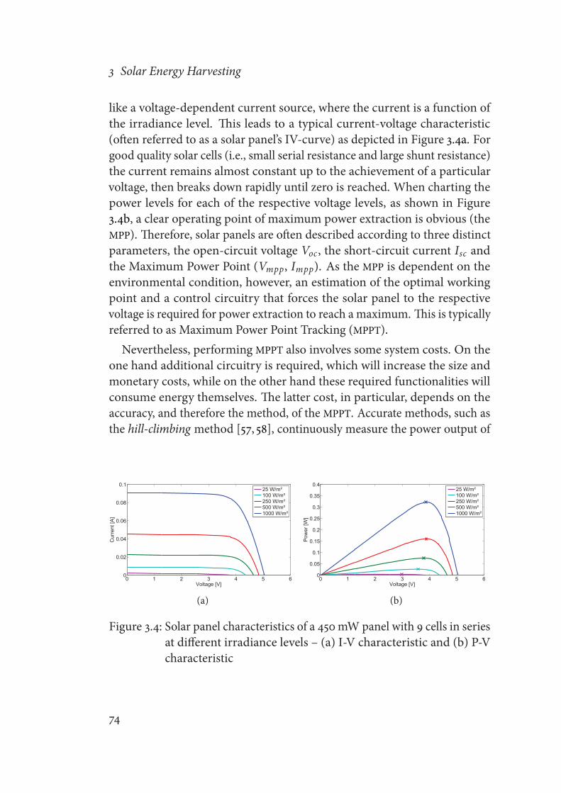
3 Solar Energy Harvesting
like a voltage-dependent current source, where the current is a function ofthe irradiance level. This leads to a typical current-voltage characteristic(often referred to as a solar panel’s IV-curve) as depicted in Figure 3.4a. Forgood quality solar cells (i.e., small serial resistance and large shunt resistance)the current remains almost constant up to the achievement of a particularvoltage, then breaks down rapidly until zero is reached. When charting thepower levels for each of the respective voltage levels, as shown in Figure3.4b, a clear operating point of maximum power extraction is obvious (theMPP). Therefore, solar panels are often described according to three distinctparameters, the open-circuit voltage Voc , the short-circuit current Isc andthe Maximum Power Point (Vmpp, Impp). As the MPP is dependent on theenvironmental condition, however, an estimation of the optimal workingpoint and a control circuitry that forces the solar panel to the respectivevoltage is required for power extraction to reach a maximum. This is typicallyreferred to as Maximum Power Point Tracking (MPPT).Nevertheless, performing MPPT also involves some system costs. On the
one hand additional circuitry is required, which will increase the size andmonetary costs, while on the other hand these required functionalities willconsume energy themselves. The latter cost, in particular, depends on theaccuracy, and therefore the method, of the MPPT. Accurate methods, such asthe hill-climbing method [57, 58], continuously measure the power output of
0 1 2 3 4 5 60
0.02
0.04
0.06
0.08
0.1
Voltage [V]
Cur
rent
[A]
25 W/m²100 W/m²250 W/m²500 W/m²1000 W/m²
(a)
0 1 2 3 4 5 60
0.05
0.1
0.15
0.2
0.25
0.3
0.35
0.4
Voltage [V]
Pow
er [W
]
25 W/m²100 W/m²250 W/m²500 W/m²1000 W/m²
(b)
Figure 3.4: Solar panel characteristics of a 450mWpanel with 9 cells in seriesat different irradiance levels – (a) I-V characteristic and (b) P-Vcharacteristic
74

3.2 Solar Energy Harvesting Architectures
the solar panel, while slowly adjusting the terminal voltage. While this allowsfor the system to operate at, or very close to, the Maximum Power Point ofthe solar panel, this method is very costly, because measurements and adjust-ments are required to be performed at a high rate. Furthermore, dependingon the step-size, the method can be rather slow to react to abrupt changes(e.g., due to abruptly changing irradiance conditions). Thus, a compromisehas to be made for the perturbation step-size, as a small step-size leads tolong reaction times, while a large step-size leads to a strong influence fromthe oscillation around the actual MPP.
Because the solar panels, which are typically used to supply sensor nodes,are of limited area and power output, the overhead costs of the MaximumPower Point Tracking solution can have a considerable impact on the systemefficiency. Therefore hill-climbing methods (also similar methods, suchas Perturb-and-Observe (PnO)) are too costly to implement. Simpler, lessaccurate methods are usually used, such as the fractional open-circuit voltageor fractional short-circuit current [59]methods. These twomethods are basedon the approximation of the relationship between the MPP and the open-circuit voltage Voc and the short-circuit current Isc to be linear. This leadsto
Vmpp ≈ kV ⋅ Voc (3.6)
Impp ≈ kI ⋅ Isc , (3.7)
where Vmpp and Impp are the voltage and current at the Maximum PowerPoint, while kV and kI are the proportionality factors, approximated as beingconstant for varying environmental conditions. However, it has to be bornein mind that this is only an approximation, as shown in Table 3.3. In this caseit can be seen that the factors kV and kI change with the irradiance level. Theachieved accuracy is still relatively good as can be seen through the effect onthe MPP estimation, shown in Figure 3.5. Estimation did occur by averagingkV and kI respectively. It can be observed that accuracies for lower irradianceconditions are worse than those for stronger irradiance. In addition, theseresults show that for the particular solar panel under test, the fractional open-circuit voltage method provides better estimations in the majority of cases.Nonetheless, the mentioned factors are solar panel dependent, meaningthat each individual panel has to be tested in order to achieve the optimaloutcome. An analysis of panels from the same type can provide an idea
75

3 Solar Energy Harvesting
of variations within the same manufacturer. If the variation is found to besmall, this could allow for some generalizations. Furthermore, although thismethod is usually less costly than the hill-climbing methods, there are stillnecessary costs associated with the performance of both measurements andadjustments. Moreover, in order to be able to react to changing irradianceconditions, sampling and adjustment rates are required to remain high.
As opposed to the input regulation, the output regulation in most systemsis rather straightforward. While systems based on Li-Ion batteries, due to theirhigh nominal voltage, might often suffice without output regulation, most
E Vmpp Impp Voc Isc kV kI[Wm−2] [V] [mA] [V] [mA]
1000 3.87 83.18 5.04 90.77 0.767 0.916500 3.88 41.34 4.84 45.39 0.810 0.910250 3.79 20.22 4.64 22.69 0.816 0.891100 3.58 7.57 4.37 9.08 0.819 0.83325 2.98 1.39 3.85 2.27 0.774 0.612
Table 3.3: Overview of measured characterization parameters of a 450mWsilicon solar panel
0 1 2 3 4 5 60
0.05
0.1
0.15
0.2
0.25
0.3
0.35
0.4
Voltage [V]
Pow
er [W
]
25 W/m²100 W/m²250 W/m²500 W/m²1000 W/m²
Figure 3.5: Accuracy of MPPT based on fractional open-circuit voltage andfractional short-circuit current; real MPP marked by cross, esti-mated from Voc marked by squares, estimated from Isc markedby circles
76

3.2 Solar Energy Harvesting Architectures
other storage types require a boost for their voltage levels in order to fulfillload demands. In the majority of cases, this involves the implementation ofa standard step-up regulator which boosts the storage voltage according to
Vout = Vstore ⋅ IstoreIout⋅ η , (3.8)
where Vout , Vstore , Iout and Istore are the voltages and currents of the energybuffer and the regulator output respectively, and η is the conversion efficiency.While consumption of these regulators can be relatively low, the converterefficiency is an important parameter for the selection process. Alternatively,multiple energy buffers can be operated in a series connection in order toincrease the output voltage. While this is rather conventional for low-voltagebatteries (e.g., NiMH, NiCd), Double Layer Capacitors can require externalcircuitry in order to allow for them to be operated in this manner.
3.2.1 Low Irradiance Conditions
While many solar energy harvesting systems for Wireless Sensor Networkshave been proposed in the literature, the majority of these systems originatefrom locations where annual solar radiation is high. Typically, with referenceto the design considerations of the systems, several hours of strong sunlightare expected each day [47, 55, 60]. This might be the case in the respectivelocations, but does not hold true in general. Figure 3.6 provides an overviewof the solar radiation during 2008 in Sundsvall, Sweden (62○24′N , 17○19′E).In locations such as these, highly unequal irradiance distributions can beobserved. While this might lead, in general, to acceptable solar radiationover the year, the solar irradiance during certain periods in the year canbe immensely low. Furthermore, even at locations where solar radiationis usually high, limited irradiance conditions can occur due to shading byobjects (e.g., trees and buildings). In situations involving frequently limitedirradiance levels, different design considerations have to be applied ratherthan those in the previously mentioned systems.Although batteries can buffer considerable amounts of energy and, thus,
supply the sensor node during long periods of weak irradiance conditions,their chemical composition and restricted lifetime makes them an undesiredtechnology for the implementation of energy buffers in solar energy harvest-
77

3 Solar Energy Harvesting
00:0004:00
08:0012:00
16:0020:00
00:00
JanFeb
MarApr
MayJun
JulAug
SepOct
NovDec
0
100
200
300
400
500
600
700
DaytimeMonth
Sol
ar ir
radi
ance
[W/m
²]
Figure 3.6: Annual solar irradiance distribution in Sundsvall, Sweden 2008;daily data averaged for each month; daytime resolution 5min
ing systems. As a result, DLC based solar energy harvesting has been analyzedfor its capabilities to be applied in low-irradiance conditions. Due to theirlimited capacity, DLCs can only be used as short-term energy buffers. As inthe targeted environments, however, relatively long periods of low-irradiancelevels are to be expected, the architecture in use has to allow for energy tobe harvested even from these weak conditions. The energy overhead of theharvesting architecture, thus, becomes one of the critical design parameters.In a first deployment, the feasibility of using DLC based harvesting archi-
tectures under low-irradiance conditions has been tested. For this evaluation,the load has been restricted to low power sensor nodes, and the main designgoal was to implement a solar energy harvesting architecture that operatesin as simple a manner as possible. The resulting architecture is depicted inFigure 3.7. The central component in the system is the Double Layer Capac-itor, which operates as the short-term energy buffer. Charging of the DLCtakes place in a rather direct manner, by having a direct coupling to the solarpanel. In order to protect the solar panel from reverse currents, however, aSchottky-diode provides the necessary directionality. Furthermore, the DLCis required to be protected from over-charge, as the solar panel can provide
78
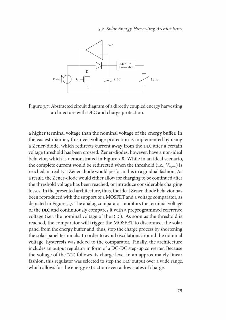
3.2 Solar Energy Harvesting Architectures
vsol ar G
S
D
DLC Load
Step-upConverter
−
+ vre f
Figure 3.7: Abstracted circuit diagram of a directly coupled energy harvestingarchitecture with DLC and charge protection.
a higher terminal voltage than the nominal voltage of the energy buffer. Inthe easiest manner, this over-voltage protection is implemented by usinga Zener-diode, which redirects current away from the DLC after a certainvoltage threshold has been crossed. Zener-diodes, however, have a non-idealbehavior, which is demonstrated in Figure 3.8. While in an ideal scenario,the complete current would be redirected when the threshold (i.e., Vnom) isreached, in reality a Zener-diode would perform this in a gradual fashion. Asa result, the Zener-diode would either allow for charging to be continued afterthe threshold voltage has been reached, or introduce considerable charginglosses. In the presented architecture, thus, the ideal Zener-diode behavior hasbeen reproduced with the support of a MOSFET and a voltage comparator, asdepicted in Figure 3.7. The analog comparator monitors the terminal voltageof the DLC and continuously compares it with a preprogrammed referencevoltage (i.e., the nominal voltage of the DLC). As soon as the threshold isreached, the comparator will trigger the MOSFET to disconnect the solarpanel from the energy buffer and, thus, stop the charge process by shorteningthe solar panel terminals. In order to avoid oscillations around the nominalvoltage, hysteresis was added to the comparator. Finally, the architectureincludes an output regulator in form of a DC-DC step-up converter. Becausethe voltage of the DLC follows its charge level in an approximately linearfashion, this regulator was selected to step the DLC output over a wide range,which allows for the energy extraction even at low states of charge.
79

3 Solar Energy Harvesting
0 Vnom0
1
VDLC
I DLC
/ I so
lar
Real Zener−DiodeIdeal Zener−Diode
Figure 3.8: Behavioral comparison of ideal and real zener-diode characteris-tics
In order to investigate the architecture’s behavior and performance, ithas been implemented with the components listed in Table 3.4. It was thendeployed in a real-world setup during the period from November 2009 toJanuary 2010 in Sundsvall, Sweden (62○24′N , 17○19′E). For the deploymentlocation, a building roof on the university campus was chosen in order toprovide an obstacle-free operation. The intention of the deployment was toobserve whether the system could supply the load during this period, whichrepresents the darkest period of the year at the chosen deployment site. Thus,correct operation would represent that the system is capable of supplying theload during the entire year. As correct operation was not guaranteed priorto the deployment, and system parameters should be monitored even if theenergy storage is depleted, the load to the solar energy harvesting system andits monitoring system have been separated. Thus, the monitoring has beenperformed with a sensor node platform, whereas the load was implementedin the form of a resistor bank, which is connected by MOSFET switches. Theload profile has been implemented in a bi-modal manner and has resultedin an average load current of 20 μA. System parameters and environmentalconditions have been digitalized and transmitted in an interval of 5min toa mains powered receiver, which forwarded the data via an General PacketRadio Service (GPRS) connection to a database server.
The deployment demonstrated that the system could supply the load overthe entire evaluation period. Both the tested DLC capacities remained abovethe threshold of approximately 0.8 V, below which the output regulationwill fail to provide a stable output. Figure 3.9 shows the behavior of the
80

3.2 Solar Energy Harvesting Architectures
Module Implementation
Solar Panel 450mW, 94 × 61mm2
DLCCooper Bussmann, C = 10 F, Vnom = 2.5VCooper Bussmann, C = 22 F, Vnom = 2.5V
Reverse Current Protection Shottky Diode (MBR0520L)
Over-Voltage Protection Comparator (MAX9017)MOSFET (MGSF2N02EL)
Output Regulator Boost (TPS61070)Load System Resistor bankMonitoring System Sentio-e2
Table 3.4: Module configuration for the implementation of the DLC-basedharvesting architecture
architecture during one week of its deployment. The results demonstratethe typical daily cycle of solar energy harvesting (Figure 3.9a), wherein theenergy storage charges during periods of sunlight and discharges when solarirradiation is absent. The charging allows for the DLC to be fully replenishedeven under low irradiance conditions, which in the presented scenario haveremained below 100Wm−2 at all times.
A limitation in this architecture can be observed with respect to the over-voltage protection of the energy buffer. The trigger point configuration of theanalog comparator involves some variation in threshold accuracy and whilethe circuitry was dimensioned in order to react to a threshold of 2.5 V, whichis the nominal voltage of the DLC in the system, the actual implementationsshowed variations from this trigger point, which resulted in a 2.45 V and2.55 V threshold for the 10 F and 22 F capacitors, respectively. Furthermore,the hysteresis of about 400mV was over-dimensioned, which resulted in abi-daily charge cycle for the 22 F DLC. Finally, the implemented method ofover-voltage protection leads to a waste of available ambient energy, as itstops harvesting energy as soon as the storage is full. Due to the additionalhysteresis, the DLC starts discharging at this point and will, in the majority ofcases, not harvest more energy during the same day. However, this behaviorreduces the stress on the DLC and, thus, is likely to increase its componentlifetime.
81

3 Solar Energy Harvesting
Day 1 Day 2 Day 3 Day 4 Day 5 Day 6 Day 7
2
2,1
2,2
2,3
2,4
2,5
Time
Term
inal
Vol
tage
[V]
22F 10F
(a)
Day 1 Day 2 Day 3 Day 4 Day 5 Day 6 Day 7
20
40
60
80
Time
Sol
ar Ir
radi
ance
[W/m
²]
(b)
Day 1 Day 2 Day 3 Day 4 Day 5 Day 6 Day 7
−10
0
10
20
Tem
pera
ture
[°C
]
Time
75
80
85
90
Hum
idity
[%]
(c)
Figure 3.9: Systembehavior of the solar energy harvesting architecture duringone week of deployment – (a) voltage level of the DLC; (b) irra-diance conditions during the week; (c) temperature and relativehumidity during the week
82

3.2 Solar Energy Harvesting Architectures
Double Layer Capacitor Thin-Film Battery
Typical capacity1 tens of F μAh to mAhVoltage range [V] 0 to 2.5 3 to 4.1
Temperature range -25 to 70 -40 to 85Internal resistance tens of mΩ tens of Ω
Recharge cycles 105 to 106 10000
Table 3.5: Property comparison of double layer capacitors and thin-film bat-teries
3.2.2 Short-Term Energy Buffers
After it was demonstrated that it is feasible to supply low-powerWireless Sen-sor Networks from solar energy harvesting architectures based on short-termenergy buffers (e.g., DLCs as previously presented), and that these architec-tures can even be utilized in low-irradiance conditions, a deeper analysis ofsuch architectures has been conducted. The energy storage technology inthese architectures has a major influence on the operation and behavior ofthe system, as individual technologies come with their respective propertiesand architectural requirements. Double Layer Capacitors and Thin-FilmBatteries have considerable lifetime advantages over conventional secondarybatteries, which becomes clear by comparing the properties of these tech-nologies, listed in Tables 3.2 and 3.5. Their limited capacity, on the other hand,allows for energy buffering to be performed only for short periods of time.Nonetheless, due to their advantageous lifetime properties, and the limitedexisting experience with these technologies in solar energy harvesting appli-cations, the comparison that is presented in this section has been focused onthese short-term energy buffers.
While Double Layer Capacitors can be charged in a simple manner, theirlow nominal voltage requires the harvesting architecture to contain a step-up regulator to match the DLC’s terminal voltage to the input requirementof the load. Furthermore, DLCs have a relatively high self-discharge rate,which reduces their capability of buffering energy for longer periods of low-irradiation. This self-discharge rate increases with increasing capacity, whichmakes the selection of a larger DLC only of limited benefit to this challenge.A recently commercialized alternative to DLCs are Thin-Film Batteries
83

3 Solar Energy Harvesting
(TFBs). While TFBs are also short-term energy buffers, their properties arequite different to those of DLCs. Table 3.5 contrasts the properties of bothdevice types, which shows that Thin-Film Batteries have a higher nominalvoltage and, thus, can avoid the usage of boost regulators. These typically havea relative high quiescent current as opposed to LDOs. In addition, the TFBshave a near-zero self-discharge, which means that harvested energy is storedmore efficiently. On the contrary, available devices are highly restricted intheir energy capacity. During the writing of this document, 2.2mAh TFBswere the largest devices, which were commercially available. Furthermore,currently available products have an internal resistance of tens of Ohms,which makes them susceptible to current peaks, such as those typically oc-curring in WSN applications. Although the amount of recharge cycles thatcan be performed is at least one magnitude lower than for DLCs, this is notconsidered a great drawback of the technology, as the number of rechargecycles of Thin-Film Batteries will be sufficient for a long system lifetime,even in the case of daily recharge cycles, which is typical for solar energyharvesting sensor nodes.In order to evaluate the impact of these properties on the actual system
operation, an experimental comparison of DLCs and TFBs, as well as theirrespective harvesting architectures, has been performed. For this, a con-figurable solar energy harvesting platform has been designed, which canbe selectively operated with DLCs or TFBs, and offers a choice of harvestingcircuits. Integrating all implementation options on one board, which can beconfigured to the desired implementation at hand, allows for the design over-head and the production cost to be kept to a minimum. The reconfigurationof a fully equipped platform is possible by simply adjusting the placement ofa group of jumpers. An architectural overview of the configurable harvestingcircuit is depicted in Figure 3.10. Overall, four different paths from the solarpanel to the load can be chosen, wherein two are using the Double LayerCapacitor and two are using the Thin-Film Battery, respectively. For eachstorage device, a minimal harvesting approach is implemented, which limitsthe circuit overhead to a minimum. In addition, a more complex energy har-vester can be utilized, which increases the overhead (i.e., circuit complexity,cost, and energy overhead), but attempts to make the charging process moreefficient by using a simplified MPPT technique.In addition to the energy harvesting circuit, the platform also contains
84
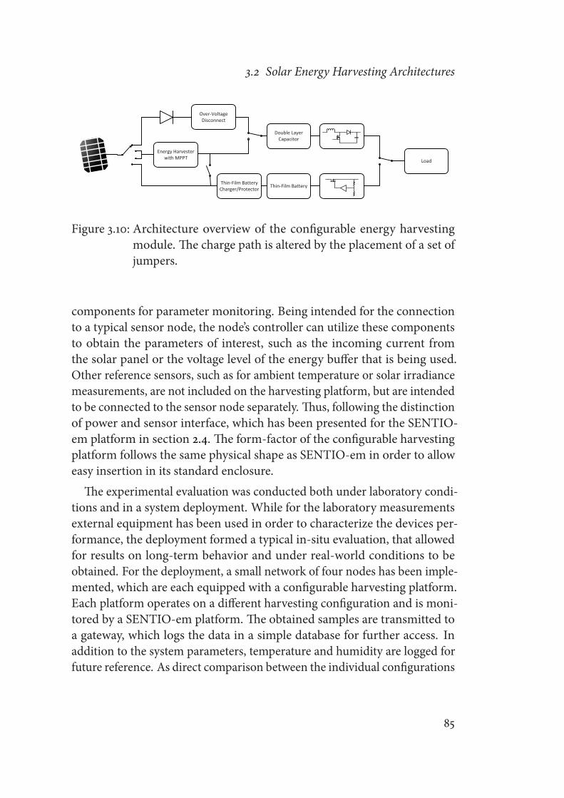
3.2 Solar Energy Harvesting Architectures
Energy Harvesterwith MPPT
Over-Voltage Disconnect
Double Layer Capacitor
Thin-Film BatteryThin-Film Battery Charger/Protector
Load
Figure 3.10: Architecture overview of the configurable energy harvestingmodule. The charge path is altered by the placement of a set ofjumpers.
components for parameter monitoring. Being intended for the connectionto a typical sensor node, the node’s controller can utilize these componentsto obtain the parameters of interest, such as the incoming current fromthe solar panel or the voltage level of the energy buffer that is being used.Other reference sensors, such as for ambient temperature or solar irradiancemeasurements, are not included on the harvesting platform, but are intendedto be connected to the sensor node separately. Thus, following the distinctionof power and sensor interface, which has been presented for the SENTIO-em platform in section 2.4. The form-factor of the configurable harvestingplatform follows the same physical shape as SENTIO-em in order to alloweasy insertion in its standard enclosure.
The experimental evaluation was conducted both under laboratory condi-tions and in a system deployment. While for the laboratory measurementsexternal equipment has been used in order to characterize the devices per-formance, the deployment formed a typical in-situ evaluation, that allowedfor results on long-term behavior and under real-world conditions to beobtained. For the deployment, a small network of four nodes has been imple-mented, which are each equipped with a configurable harvesting platform.Each platform operates on a different harvesting configuration and is moni-tored by a SENTIO-em platform. The obtained samples are transmitted toa gateway, which logs the data in a simple database for further access. Inaddition to the system parameters, temperature and humidity are logged forfuture reference. As direct comparison between the individual configurations
85
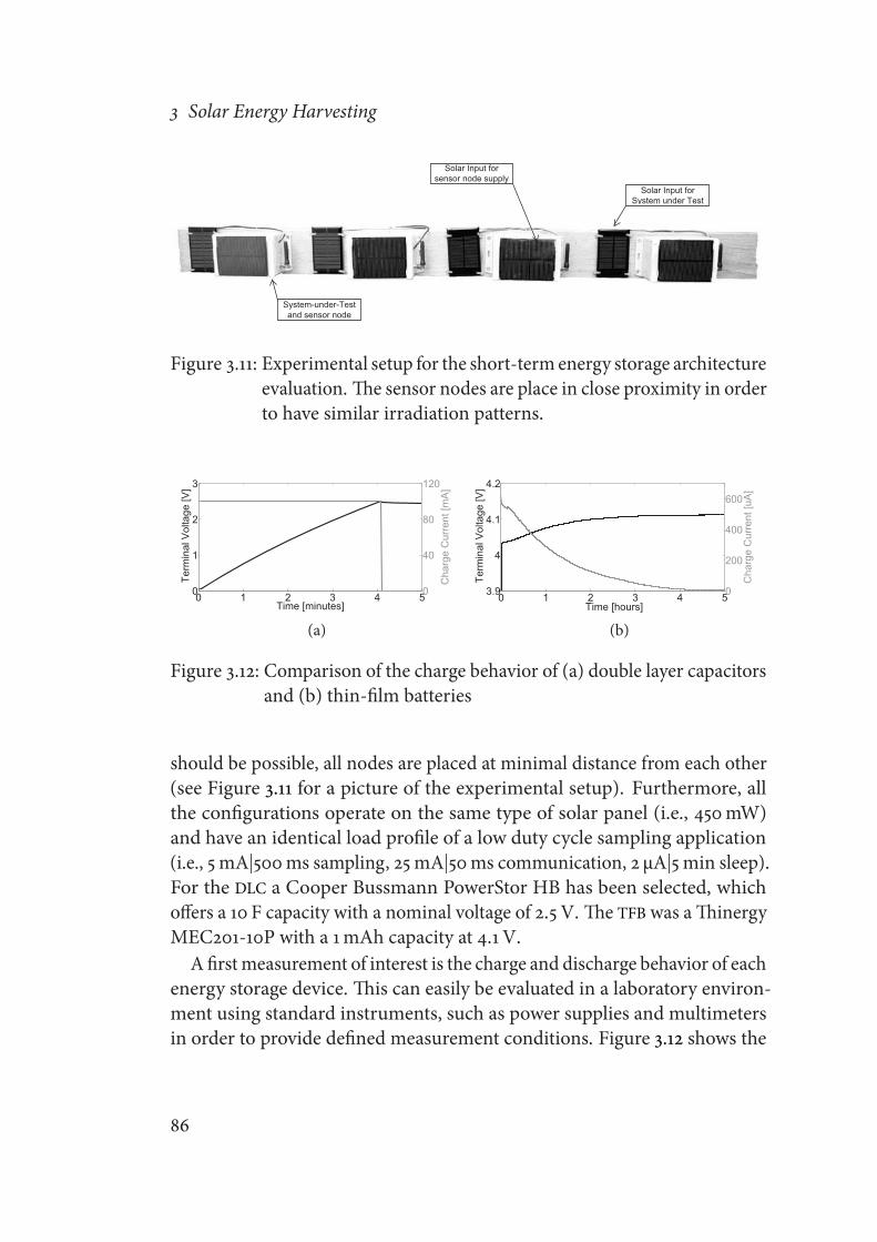
3 Solar Energy Harvesting
Solar Input forSystem under Test
System-under-Testand sensor node
Solar Input forsensor node supply
Figure 3.11: Experimental setup for the short-term energy storage architectureevaluation. The sensor nodes are place in close proximity in orderto have similar irradiation patterns.
0 1 2 3 4 50
1
2
3
Time [minutes]
Term
inal
Vol
tage
[V]
0
40
80
120
Cha
rge
Cur
rent
[mA
]
(a)
0 1 2 3 4 53.9
4
4.1
4.2Te
rmin
al V
olta
ge [V
]
0
200
400
600
Time [hours]
Cha
rge
Cur
rent
[uA
]
(b)
Figure 3.12: Comparison of the charge behavior of (a) double layer capacitorsand (b) thin-film batteries
should be possible, all nodes are placed at minimal distance from each other(see Figure 3.11 for a picture of the experimental setup). Furthermore, allthe configurations operate on the same type of solar panel (i.e., 450mW)and have an identical load profile of a low duty cycle sampling application(i.e., 5mA∣500ms sampling, 25mA∣50ms communication, 2 μA∣5min sleep).For the DLC a Cooper Bussmann PowerStor HB has been selected, whichoffers a 10 F capacity with a nominal voltage of 2.5 V. The TFB was aThinergyMEC201-10P with a 1mAh capacity at 4.1 V.
A firstmeasurement of interest is the charge and discharge behavior of eachenergy storage device. This can easily be evaluated in a laboratory environ-ment using standard instruments, such as power supplies and multimetersin order to provide defined measurement conditions. Figure 3.12 shows the
86

3.2 Solar Energy Harvesting Architectures
0 1 2 31.768
1.770
1.772
1.774
Time [minutes]
Term
inal
Vol
tage
[V]
(a)
0 1 2 3 43
3.2
3.4
3.6
3.8
4
Time [seconds]
Term
inal
Vol
tage
[V]
(b)
Figure 3.13: Peak discharge behavior of (a) double layer capacitors and (b)thin-film batteries
charge behavior of both devices under conditions that are similar to strongirradiance using the previously mentioned solar panel (i.e., current-limited at100mA). The DLC shows a nearly linear voltage increase over time, whereasthe TFB has a non-linear behavior with only a small change in terminal volt-age. The obtained measurements confirm the negative influence of the highinternal resistance in the TFBs, which results in much smaller charge currentsthan are available from the power supply. While the DLC constantly draws themaximal available charge current from the source, the TFB’s charge current islimited to a few hundred microampere. Thus, these devices require relativelylong periods of irradiation as compared to the DLCs in order to replenishtheir energy reservoir.Another influence of the internal resistance can be observed in the dis-
charge behavior. As was previously mentioned, Wireless Sensor Networkstypically pose a bi-modal load profile on their power supplies, which con-tains long periods with near-zero consumption, but which are interruptedwith periodically occurring peaks of relative high consumption. Figure 3.13depicts the behavior of the energy buffers when being exposed to such aload profile. In a similar manner to that during the charging, the effect onthe DLC is minimal due to its low internal resistance, whereas the TFB showsa considerable reaction to the applied load peaks. In order to prevent theload system from being reset, large capacitors have to be utilized in orderto maintain an appropriate supply voltage. The high resistance of TFBs, thus,affects both charging and discharging characteristics in a negative manner.Finally, the system has been deployed in an evaluation network for the
87
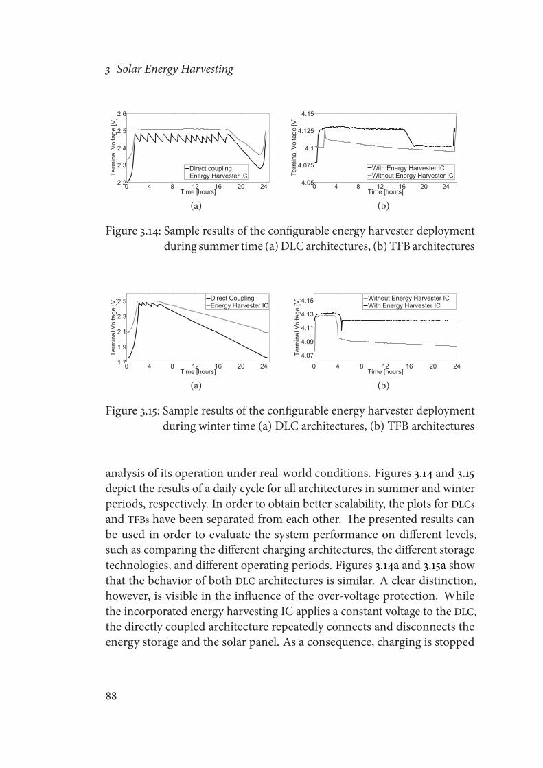
3 Solar Energy Harvesting
0 4 8 12 16 20 242.2
2.3
2.4
2.5
2.6
Time [hours]
Term
inal
Vol
tage
[V]
Direct couplingEnergy Harvester IC
(a)
0 4 8 12 16 20 244.05
4.075
4.1
4.125
4.15
Time [hours]
Term
inal
Vol
tage
[V]
With Energy Harvester ICWithout Energy Harvester IC
(b)
Figure 3.14: Sample results of the configurable energy harvester deploymentduring summer time (a)DLC architectures, (b) TFB architectures
0 4 8 12 16 20 241.7
1.9
2.1
2.3
2.5
Time [hours]
Term
inal
Vol
tage
[V] Direct Coupling
Energy Harvester IC
(a)
0 4 8 12 16 20 24
4.07
4.09
4.11
4.13
4.15
Time [hours]
Term
inal
Vol
tage
[V] Without Energy Harvester IC
With Energy Harvester IC
(b)
Figure 3.15: Sample results of the configurable energy harvester deploymentduring winter time (a) DLC architectures, (b) TFB architectures
analysis of its operation under real-world conditions. Figures 3.14 and 3.15depict the results of a daily cycle for all architectures in summer and winterperiods, respectively. In order to obtain better scalability, the plots for DLCsand TFBs have been separated from each other. The presented results canbe used in order to evaluate the system performance on different levels,such as comparing the different charging architectures, the different storagetechnologies, and different operating periods. Figures 3.14a and 3.15a showthat the behavior of both DLC architectures is similar. A clear distinction,however, is visible in the influence of the over-voltage protection. Whilethe incorporated energy harvesting IC applies a constant voltage to the DLC,the directly coupled architecture repeatedly connects and disconnects theenergy storage and the solar panel. As a consequence, charging is stopped
88

3.2 Solar Energy Harvesting Architectures
prematurely in this architecture, which leads to a faster voltage decrease rateduring periods of no irradiation. Similarly, a difference can be observedbetween the charge methods of the TFBs (Figures 3.14b, 3.15b). As theThin-Film Batteries have a relatively high nominal voltage of the order of 4V, theyrequire a relatively high terminal voltage in order to be charged. The utilizedsolar panel, however, will only deliver an appropriate voltage if irradiation ishigh. In situations when the irradiation is not sufficiently strong, the TFB canbenefit from the harvesting IC, as it boosts the voltage from the solar panelbefore it is applied to the energy storage device. Comparing, on the otherhand, the DLC based architectures with those using a TFB, the differences aremore profound. While on first view, the general behavior is similar, thusthere is a higher voltage during daylight and lower/reducing voltage duringdarkness, the previously presented laboratory results can be used in orderto explain some of the differences. In the case of the DLC, terminal voltagechanges accurately with the state of charge and, hence, a slower increaseand decrease rate can be observed in the graphs, despite the much highercharge currents, which can be achieved with this energy buffer. For the TFB,in contrast, terminal voltage changes much less with regards to the state ofcharge, whereas the major influence on the voltage is determined by the solarpanel’s voltage due to the high internal resistance of the TFB. In addition tothe effect on charge and discharge behavior, this presents another limitingfactor of TFBs, as it makes the estimation of the state of charge a difficultprocess. Finally, the seasonal influence on the system behavior follows theexpectations. All figures clearly indicate the differences in daylight periodsbetween summer (Figure 3.14) and winter (Figure 3.15) due to the resultingdifferences in terminal voltages.
Although the previously presented results suggest that using the energyharvester IC improves the system operation, this is not the case in each andevery situation. Figure 3.16 depicts the results of the two DLC architecturesduring a period of extremely low irradiation during the winter. The voltagecurves show that the directly coupled architecture has a benefit in relation tothese conditions, because its overhead is low in comparison to the energyharvesting IC. Furthermore, the utilized IC uses a simple MPPT method, andthese methods have been demonstrated to be inaccurate, particularly underlow irradiance conditions.
89

3 Solar Energy Harvesting
0 12 24 36 481.7
1.9
2.1
2.3
2.5
Time [hours]Te
rmin
al V
olta
ge [V
]
Direct CouplingEnergy Harvester IC
Figure 3.16: MPPT utilization during periods of low irradiation for DLC basedenergy harvesting systems
3.3 Solar Energy Harvesting Dimensioning
While, in general, because of their inexhaustible energy source, solar energyharvesting systems allow for a perpetual energy supply, energy harvestingsystems are limited by the supply rate, as was previously mentioned. More-over, this rate limitation is spatially and temporally dependent. Thus, anenergy neutral operation is only possible when supply rate conditions andconsumption conditions are met. The proper planning of the solar energyharvesting system becomes an essential part in the design process. Figure3.17 provides an overview of the constraint factors involved in solar energyharvesting systems. The goal in relation to system planning is to determinea set of required constraints under otherwise given constraints. A typicalexemplary case would be the determination of the necessary harvester di-mensions (e.g., solar panel rating and energy storage capacity), while theenvironmental and application constraints are fixed.
This component dimensioning is necessary for harvesting systems, regard-less of the particular architecture chosen. Taking the architectures presentedin the previous section as an example, straightforward parameters includeDLC capacity and solar panel size. The choice of these parameters dependsmainly on the power profile of the system load and the environmental condi-tions at the intended location (i.e., especially the irradiance levels). Whileon the one hand, under-dimensioning leads to unreliable operation, over-dimensioning is also undesirable as it leads to an unnecessary increase inboth the size and cost of the system. Even though a systematic method ofdimensioning system components is desired, the complexity of the system
90

3.3 Solar Energy Harvesting Dimensioning
Application Constraints
Envir
onm
ent
Con
stra
ints
Harvester
Constraints
Figure 3.17: Overview of constraint sources, influencing each other, in energyharvesting systems
and the challenge of simplifying location-based influences makes analyticalapproaches difficult to handle. Using a system model of the underlying archi-tecture in order to simulate the State-of-Charge for given conditions, allowsfor the components of the architecture to be dimensioned. The possibilityand performance of this type of dimensioning method will be demonstratedin the following section, using the directly-coupled architecture (as in Figure3.7) as a case example.
3.3.1 Modeling of the Solar Energy Harvesting Architecture
Figure 3.18 provides an overview of the main interactions in the target archi-tecture, which results in its system behavior. Because of the direct couplingbetween the solar panel and DLC, the voltage of the solar panel will followthe voltage of the energy buffer (with a small offset due to the reverse currentprotection diode). At the same time, however, the charge current dependson the irradiance level. Thus, the operating point of the solar panel, at anypoint in time, is given by the irradiance and the DLC charge level. In return,this operating point defines the charge-rate of the DLC, changing its voltagelevel over time, leading again to a change of the operating point of the solarpanel. Additionally, the DLC is discharged continuously by the load system ata rate defined by the load’s energy profile. This leads, in combination withthe incoming energy from the solar panel, to an overall charge or dischargecondition.
91
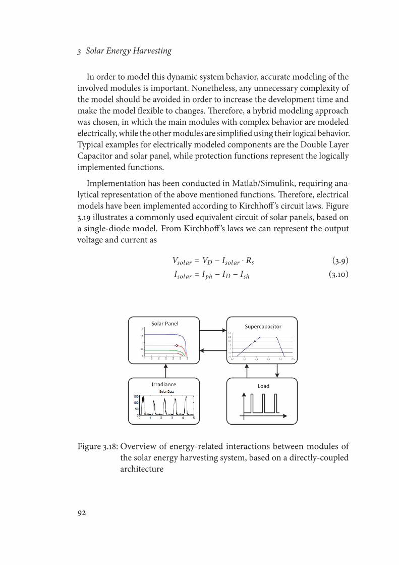
3 Solar Energy Harvesting
In order to model this dynamic system behavior, accurate modeling of theinvolved modules is important. Nonetheless, any unnecessary complexity ofthe model should be avoided in order to increase the development time andmake the model flexible to changes. Therefore, a hybrid modeling approachwas chosen, in which the main modules with complex behavior are modeledelectrically, while the othermodules are simplified using their logical behavior.Typical examples for electrically modeled components are the Double LayerCapacitor and solar panel, while protection functions represent the logicallyimplemented functions.
Implementation has been conducted in Matlab/Simulink, requiring ana-lytical representation of the above mentioned functions. Therefore, electricalmodels have been implemented according to Kirchhoff ’s circuit laws. Figure3.19 illustrates a commonly used equivalent circuit of solar panels, based ona single-diode model. From Kirchhoff ’s laws we can represent the outputvoltage and current as
Vsolar = VD − Isolar ⋅ Rs (3.9)Isolar = Iph − ID − Ish (3.10)
Irradiance
Solar Panel Supercapacitor
Load
Figure 3.18: Overview of energy-related interactions between modules ofthe solar energy harvesting system, based on a directly-coupledarchitecture
92

3.3 Solar Energy Harvesting Dimensioning
iph vd
id
Rsh
ish
Rsis
vsol ar
Figure 3.19: Equivalent circuit of a solar panel according to the single-diodemodel
with the notations as indicated in Figure 3.19. Using (3.9) in (3.10) and replac-ing ID with Shockeley’s diode equation, leads to a more detailed descriptionof the resulting output current
Isolar = Iph − I0 ⋅ (e q(Vsol ar+Isol ar ⋅Rs)nkT − 1) − Vsolar + Isolar ⋅ Rs
Rsh, (3.11)
where Iph can be deduced as being proportional to the irradiance level, suchas
Iph = kirr ⋅ E . (3.12)
Substituting Iph in (3.11) with (3.12), the solar panel model is implementableusing standard operations. This leaves the key modeling parameters as beingthe serial resistance Rs, the shunt resistance Rsh, the irradiance level E, aswell as the proportionality factor kirr . With the exception of the irradiance,these parameters are solar panel properties and can be determined by variousmethods, e.g. by analyzing I-V curve characteristics, such as proposed in [61].
Similarly, the DLC can be implemented according to a voltage and currentanalysis of the equivalent circuit, shown in Figure 3.20. The circuit shows atwo-branch model, which has been introduced in [62]. The two branchesrepresent the short-term (R0,C0, kv ⋅ V) and long-term behaviors (R2,C2)of the DLC respectively, while leakage is modeled by means of an additionalEquivalent Parallel Resistance (EPR). Following the currents and voltages as
93

3 Solar Energy Harvesting
vd l c
id l c
R0
i1
C0 kv ⋅ V
R2
i2
C2
EPR
i3
Figure 3.20: Equivalent circuit of a double layer capacitor according to thetwo-branch model
described in Figure 3.20, we can describe the model by means of
IDLC = I1 + I2 + I3 (3.13)
VDLC = I1 ⋅ R0 + ∫ I1C0 + KV ⋅ VDLC
dt (3.14)
VDLC = I2 ⋅ R2 + 1C2∫ I2 dt (3.15)
VDLC = I3 ⋅ EPR (3.16)
In this case, R0, C0, KV , R2, C2 and EPR are constants and can be determinedaccording to the description presented in [62]. The determination of theseparameters, however, has to be repeated for every type and size of DLC to beused in simulations, as simple deduction is not feasible.
Implementing the twomainmodules and filling connections between themby adding logical representations of protection mechanisms, it is possible toproduce a system model of the energy harvesting power supply. At a highabstraction level, this system model can be described as depicted in Figure3.21. While architectural parameters are defined inside the system model,such as solar panel type or DLC capacity, external conditions are provided asinputs to the model. The final output of the model is the voltage level of theDouble Layer Capacitor at any simulation point, which allows for there to bean estimate for the amount of time when there is insufficient energy under
94

3.3 Solar Energy Harvesting Dimensioning
Solar Energy Harvesting System
Model
Duty Cycle
Temperature
Solar Irradiance
DLC Voltage
Figure 3.21: Overview of the solar energy harvesting system model on highabstraction level
0 20 40 60 80 100 120
2
2,1
2,2
2,3
2,4
2,5
2,6
Time [hours]
Cap
acito
r vol
tage
[V] Simulated
Measured
(a)
0 20 40 60 80 100 1202.2
2.3
2.4
2.5
2.6
Time [hours]
Cap
acito
r vol
tage
[V] Simulated
Measured
(b)
Figure 3.22: Evaluation of energy levels estimated by the system model com-pared to deployment results – configured with (a) a 10 F DLCand (b) a 22 F DLC
given conditions.
3.3.2 Simulating Available Energy Levels
Before the model was used for simulations, an evaluation has been conductedagainst a real-world deployment of the same architecture, as was describedin Section 3.2.1. The results of the measured energy level and estimatedenergy level from the model for one week of operation are shown in Figure3.22. In the deployment two different DLC capacities have been implemented,leading to results from a 10 F version, shown in Figure 3.22a and results froma 22 F version in Figure 3.22b. While for both cases the evaluation showsthat the simulations and measurements generally conform well, smaller errorsources can be detected. This is visible especially in Figure 3.22a, where sometime-shifts can be observed. It was found that, this is the result of slightlyvarying hysteresis bounds. While the model can be adjusted to average
95

3 Solar Energy Harvesting
Parameter Optimization Goal
Solar panel size Minimization of cost and sizeDLC capacity Minimization of cost and sizeLoad consumption Maximization of duty cycle (sampling rate)Solar irradiance Minimization of environmental dependencyLoad availability Maximization of system uptimeHysteresis band Minimization of component stress
Table 3.6: Dimensioning parameters of the example solar energy harvestingarchitecture with their respective optimization goals
hysteresis bound levels, variations in the trigger level related to environmentalconditions are very difficult to predict. In Figure 3.22b a difference at thesawtooth tip is obvious. However, this does not result from a modeling errorof the energy harvesting system, but from a measurement error, due to alimited measurement range of up to 2.5 V. The evaluation confirmed that themodel is capable of predicting the SOC in an accurate manner.
After the model was evaluated, it has been used in order to demonstrate itspurpose to support the optimization process of parameter dimensioning. Anumber of parameters of interest to be optimized for the example architectureare listed in Table 3.6. While typically, not all the optimization goals can bemet simultaneously, the simulations enable the discovery of trade-offs, whichmeet the given application requirements. An exemplar simulation outcomefor the presented system architecture is shown in Figure 3.23. The depictedresults have been obtained using two assumptions:
1. Solar panel size is perfectly scalable, meaning that an increase of solarpanel size leads to an increase by the same factor in irradiance-to-current conversion at the same voltage.
2. At times of insufficient energy (i.e., the voltage level of the DLC is lowerthan the minimal boost converter input) the load will consume noenergy.
Furthermore, all the simulations are based on the irradiance data of De-cember 2009 in Sundsvall, Sweden, which is the darkest month of the year.
96
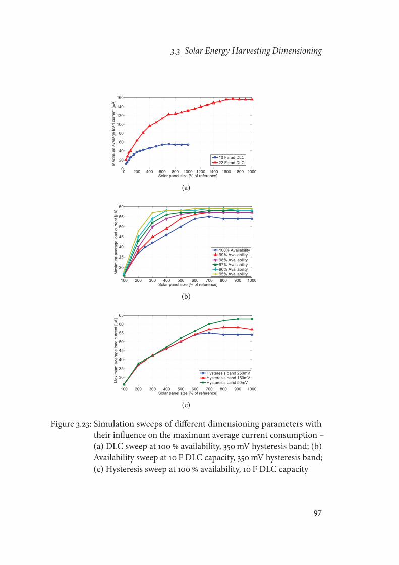
3.3 Solar Energy Harvesting Dimensioning
0 200 400 600 800 1000 1200 1400 1600 1800 20000
20
40
60
80
100
120
140
160
Solar panel size [% of reference]
Max
imum
ave
rage
load
cur
rent
[�A
]
10 Farad DLC22 Farad DLC
(a)
100 200 300 400 500 600 700 800 900 1000
30
35
40
45
50
55
60
Solar panel size [% of reference]
Max
imum
ave
rage
load
cur
rent
[�A
]
100% Availability99% Availability98% Availability97% Availability96% Availability95% Availability
(b)
100 200 300 400 500 600 700 800 900 1000
30
35
40
45
50
55
60
65
Solar panel size [% of reference]
Max
imum
ave
rage
load
cur
rent
[�A
]
Hysteresis band 250mVHysteresis band 150mVHysteresis band 50mV
(c)
Figure 3.23: Simulation sweeps of different dimensioning parameters withtheir influence on the maximum average current consumption –(a) DLC sweep at 100% availability, 350mV hysteresis band; (b)Availability sweep at 10 F DLC capacity, 350mV hysteresis band;(c) Hysteresis sweep at 100% availability, 10 F DLC capacity
97

3 Solar Energy Harvesting
The results show the maximum allowable load current (i.e., the average cur-rent consumption) under varying system configurations. All sub-figuresinclude variations of the solar panel size as a typical parameter which is tobe changed. Additionally, Figure 3.23a shows the impact of a change in DLCcapacity, Figure 3.23b the change of availability requirements and Figure 3.23cthe variation of the hysteresis band setting of the over-voltage protectioncircuit. The information from these simulations can be used in order to selectappropriate system parameters for a given application scenario.In particular, these results can support decisions for system designers.
Taking Figure 3.23b as an example, it can be extracted that it is not reasonableto increase the solar panel size by more than a factor of three, when lifetime isthe constraint with an availability factor of 95%. At the same time, trade-offdecisions can bemade, such as determining, that a 45 μA average load currentconstraint can be reached with a 96% availability and double solar panel size,or with a 99% availability, combined with a triple-sized solar panel.
3.4 Solar Energy Harvesting Testbed
While the feasibility of using solar energy harvesting architectures as thepower supply of wireless sensor nodes has been demonstrated, and energylevel simulations have been presented as a suitable method of dimensioningthese architectures, extensive experiments are required in order to evaluatearchitectures and create accurate system models. These experiments are timeand cost consuming, due to the required network deployment, which hasbeen accepted by the research community as an extremely difficult process[13]. The evaluations to be performed, such as those presented in the previoussections, are therefore limited to a subset of test cases, which results in a trade-off between time and cost expense and the desired evaluations to be carriedout. In relation to solar energy harvesting architectures, test cases of interestinclude any variation that can be performed to the system as depicted inFigure 3.2. These includemajor variations, such as the comparison of differentcharging architectures and storage technologies, but at the same time minorchanges, such as storage capacities, solar panel sizes and load profiles, may beof interest. In particular, minor variations will suffer from the considerableoverhead required for their consideration in real-world experiments.
98
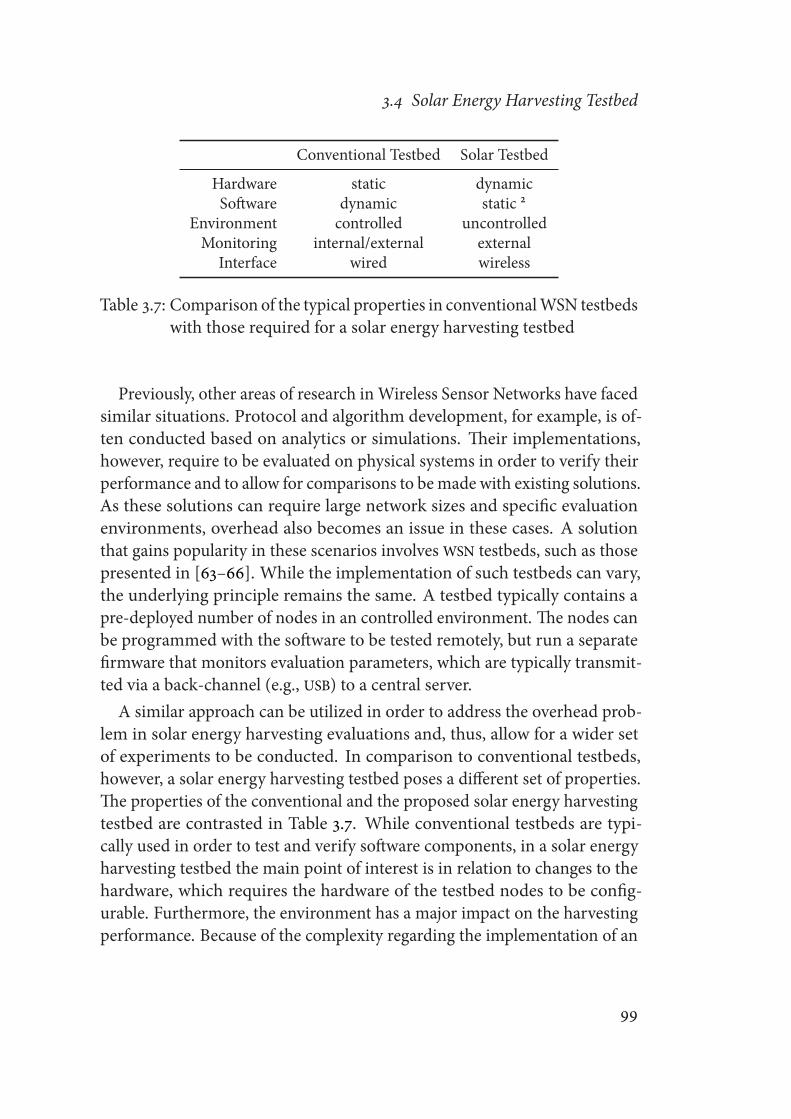
3.4 Solar Energy Harvesting Testbed
Conventional Testbed Solar Testbed
Hardware static dynamicSoftware dynamic static 2
Environment controlled uncontrolledMonitoring internal/external external
Interface wired wireless
Table 3.7: Comparison of the typical properties in conventionalWSN testbedswith those required for a solar energy harvesting testbed
Previously, other areas of research inWireless Sensor Networks have facedsimilar situations. Protocol and algorithm development, for example, is of-ten conducted based on analytics or simulations. Their implementations,however, require to be evaluated on physical systems in order to verify theirperformance and to allow for comparisons to bemade with existing solutions.As these solutions can require large network sizes and specific evaluationenvironments, overhead also becomes an issue in these cases. A solutionthat gains popularity in these scenarios involves WSN testbeds, such as thosepresented in [63–66]. While the implementation of such testbeds can vary,the underlying principle remains the same. A testbed typically contains apre-deployed number of nodes in an controlled environment. The nodes canbe programmed with the software to be tested remotely, but run a separatefirmware that monitors evaluation parameters, which are typically transmit-ted via a back-channel (e.g., USB) to a central server.
A similar approach can be utilized in order to address the overhead prob-lem in solar energy harvesting evaluations and, thus, allow for a wider setof experiments to be conducted. In comparison to conventional testbeds,however, a solar energy harvesting testbed poses a different set of properties.The properties of the conventional and the proposed solar energy harvestingtestbed are contrasted in Table 3.7. While conventional testbeds are typi-cally used in order to test and verify software components, in a solar energyharvesting testbed the main point of interest is in relation to changes to thehardware, which requires the hardware of the testbed nodes to be config-urable. Furthermore, the environment has a major impact on the harvestingperformance. Because of the complexity regarding the implementation of an
99

3 Solar Energy Harvesting
Environmental Conditions
Configuration
Monitoring
Devices under Test Data Management
Figure 3.24: Conceptual overview of the solar energy harvesting testbed. Anetwork of configurable devices is deployed in order to be ex-posed to varying environmental conditions.
artificial environment to be controlled for all scenarios of interest, a morerealistic approach is for the system to be deployed in an outdoor environment,which is uncontrolled, but provides a wide range of real-world conditions.The monitoring of environmental parameters, thus, becomes of high impor-tance in order to make sense out of the system data that has been collected. Inaddition, the outdoor deployment makes wired back-channeling infeasible,but favors the use of a wireless collection and control method.
The resulting system concept is depicted in Figure 3.24. A network ofsensor nodes with configurable solar energy harvesting is deployed in anenvironment, which exposes the system to varying environmental conditions.The nodes are remotely configured in order to define the solar energy har-vesting method and system conditions, which are to be evaluated. Moreover,the wireless link is utilized in order to obtain the parameters of the systembehavior and its surrounding. As a result of this concept, the amount ofarchitectures and configurations to be tested is much larger than the numberof system components that have to be deployed. Hence, the testbed reducesoverhead in the experimental setup as compared to that for a conventionalevaluation network. The distributed architecture of the testbed, furthermore,allows for direct comparisons of architectures and locations to be performed.
100
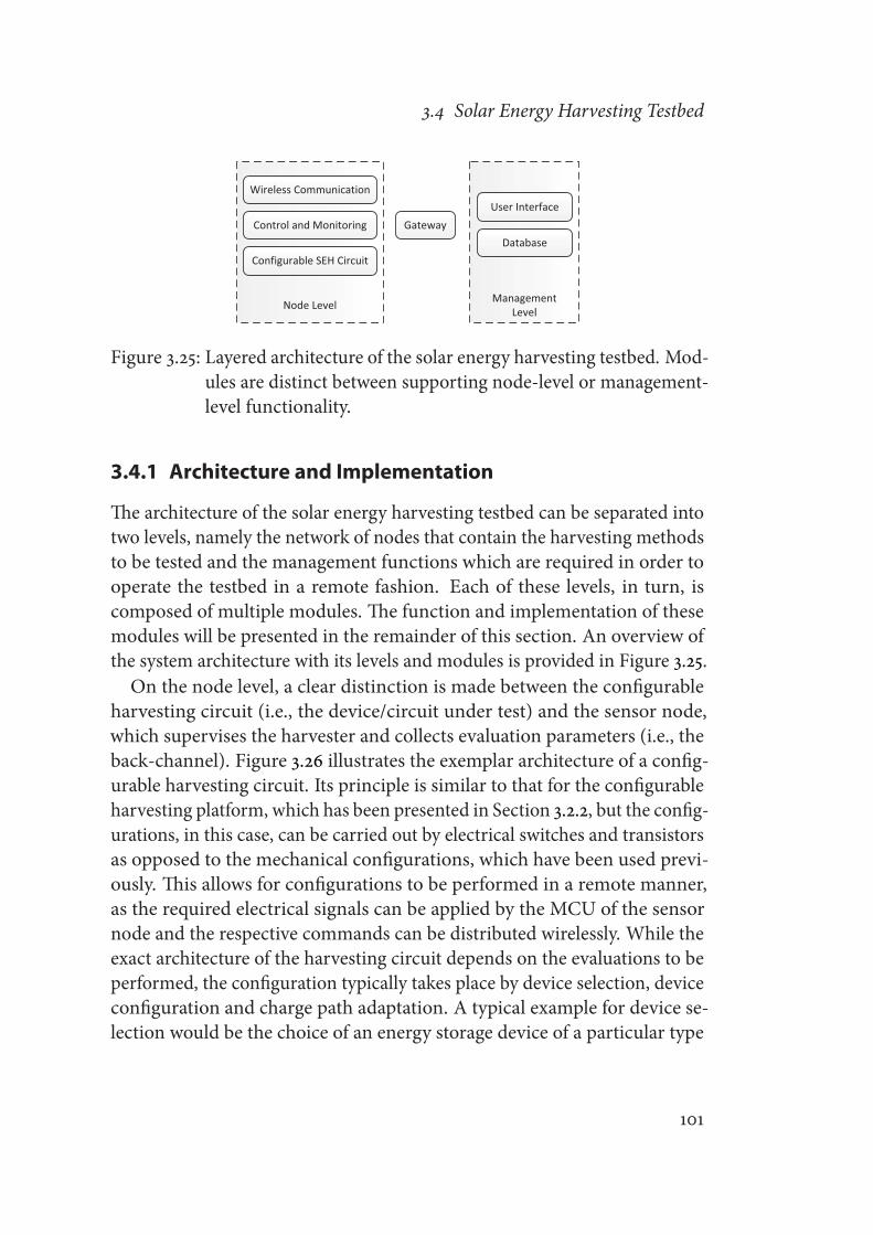
3.4 Solar Energy Harvesting Testbed
Configurable SEH Circuit
Control and Monitoring
Wireless Communication
GatewayDatabase
User Interface
Node Level Management Level
Figure 3.25: Layered architecture of the solar energy harvesting testbed. Mod-ules are distinct between supporting node-level or management-level functionality.
3.4.1 Architecture and Implementation
The architecture of the solar energy harvesting testbed can be separated intotwo levels, namely the network of nodes that contain the harvesting methodsto be tested and the management functions which are required in order tooperate the testbed in a remote fashion. Each of these levels, in turn, iscomposed of multiple modules. The function and implementation of thesemodules will be presented in the remainder of this section. An overview ofthe system architecture with its levels and modules is provided in Figure 3.25.On the node level, a clear distinction is made between the configurable
harvesting circuit (i.e., the device/circuit under test) and the sensor node,which supervises the harvester and collects evaluation parameters (i.e., theback-channel). Figure 3.26 illustrates the exemplar architecture of a config-urable harvesting circuit. Its principle is similar to that for the configurableharvesting platform, which has been presented in Section 3.2.2, but the config-urations, in this case, can be carried out by electrical switches and transistorsas opposed to the mechanical configurations, which have been used previ-ously. This allows for configurations to be performed in a remote manner,as the required electrical signals can be applied by the MCU of the sensornode and the respective commands can be distributed wirelessly. While theexact architecture of the harvesting circuit depends on the evaluations to beperformed, the configuration typically takes place by device selection, deviceconfiguration and charge path adaptation. A typical example for device se-lection would be the choice of an energy storage device of a particular type
101

3 Solar Energy Harvesting
Solar Panel #1
Solar Panel #2
Solar Panel #3
Charging Circuitry
Battery
DLC#1
DLC#2
DLC#3
Regulation Load Emulation
Configuration ConfigurationSelection Selection
Figure 3.26: Architecture of the configurable energy harvesting module ofthe solar energy harvesting testbed nodes. Configurations areperformed by electrical signals.
and capacity, device configuration might be the adjustment of a setting ata harvesting IC, whereas the charge path adaptation defines which of theprovided components are involved in the evaluation circuit and in what or-der the components are placed in order to construct a charge path. In theexemplar implementation (Figure 3.26), configurations can be performedto all modules within the solar energy harvesting circuit (see Figure 3.2 forgeneral reference). The system enables there to be a variety of different so-lar panel and energy storage choices in order to test the influence of solarpanel size/rating, as well as energy storage type and storage capacity. Withregards to the input regulation, a commercial harvesting IC has been chosen,which can be configured to different output voltages and allows for MPPTto be enabled or disabled. Although different output regulation modulesare integrated in the system, the choice is not a user configuration, but isdependent on the selection of the energy buffer type. Finally, the architectureallows for different load conditions to be tested. This has been accomplishedby means of a resistive load emulation, which allows for the load profile to beemulated by creating defined power peaks for configurable periods of time.As was mentioned previously, this implementation does not attempt to allowfor every evaluation that is of interest in a solar energy harvesting system tobe performed, but rather shows the principle of how a remotely configurablearchitecture might be implemented.The control and monitoring of the configurable harvesting circuit is per-
formed by a typical sensor node platform (i.e., in this implementation a
102

3.4 Solar Energy Harvesting Testbed
SENTIO-em platform). Additional interfaces are, however, integrated inthe harvesting circuitry, which enables the node to perform the samplingof evaluation parameters, such as current flows and voltage levels. Thesevalues can be utilized in order to correlate the influence of environmentalconditions with the system behavior of the harvester under test, as well asto estimate the operation state of the circuit (e.g., the charge level of theenergy buffer) at any given time. In addition to a number of system internalparameters, the sensor node is responsible for the measurement of referencevalues, such as for the classification of the environmental conditions duringthe evaluation period. In the exemplar implementation, reference values areobtained in the form of temperature, humidity and solar irradiance.
Using a conventional sensor node for the control and monitoring, it addi-tionally provides an existing interface for communication and networking– including the respective protocols – to the testbed nodes. This interfaceis used, on the one hand, to distribute the configurations to the individualnodes and, on the other hand, to collect the sampled parameters in a centrallocation, which is the basis for the management level.
Because available energy is one of the key parameters for the evaluation ofan energy harvesting architecture, a clear separation is required between theenergy source to be tested and the energy source that supplies the monitoringand control functionalities. Therefore, a two-domain architecture has beenchosen for the testbed nodes. While the system to be tested is poweredfrom its own resources, all modules, which are only for the observation andconfiguration of the system, are supplied from an additional source. Thesemodules include all switches for the reconfiguration of the harvester, thereference sensors, as well as the sensor node supply (i.e., all intelligence andcommunication). The backbone power supply, in this system, should bedimensioned to guarantee continuous operation. In the implementation,this has been accomplished with an off-the-shelf combination of solar panel,charge regulator and high-capacity battery, which can supply a testbed nodefor approximately two months without solar energy income.Management functions include the data storage, which is typically per-
formed by a database system, and the user interface. In the implementedsystem, the database acts as the central buffer. The gateway uses the databaseto store all parameters that have been collected from the testbed and forwardsconfigurations that are stored in the database to the testbed nodes. Similarly,
103
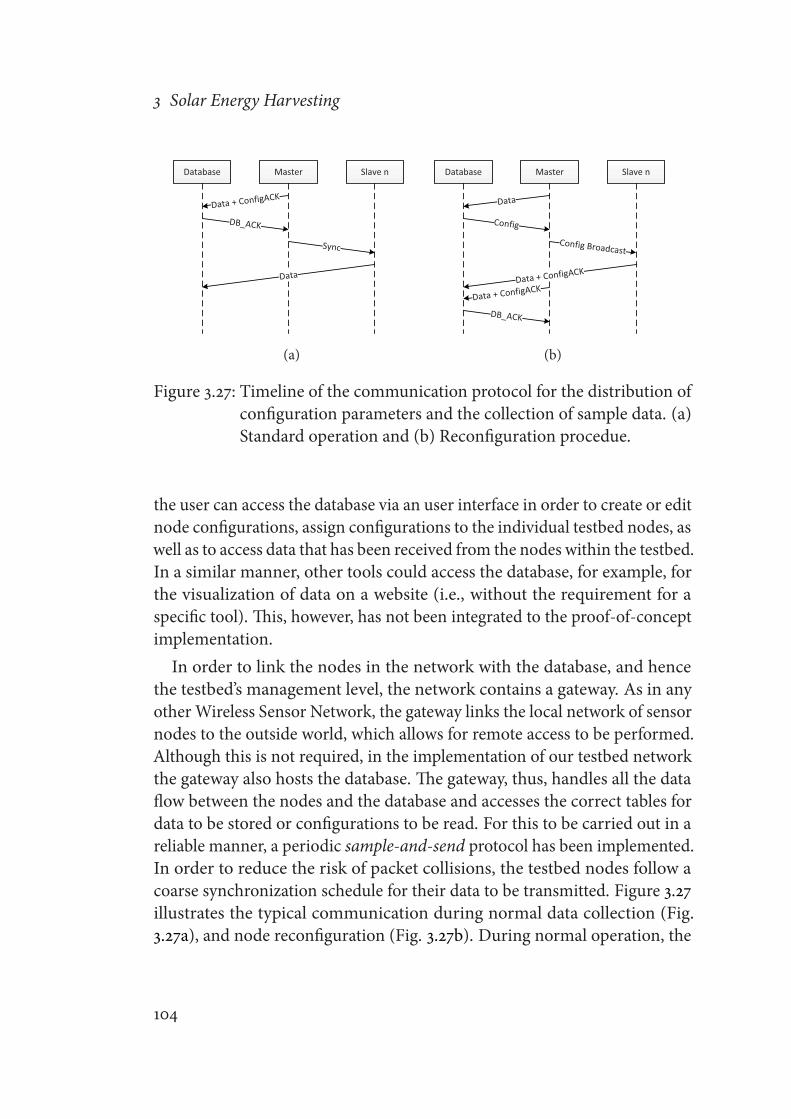
3 Solar Energy Harvesting
Database Master Slave n
Data + ConfigACK
DB_ACK
Sync
Data
(a)
Database Master Slave n
Data
Config
Config Broadcast
Data + ConfigACK
Data + ConfigACK
DB_ACK
(b)
Figure 3.27: Timeline of the communication protocol for the distribution ofconfiguration parameters and the collection of sample data. (a)Standard operation and (b) Reconfiguration procedue.
the user can access the database via an user interface in order to create or editnode configurations, assign configurations to the individual testbed nodes, aswell as to access data that has been received from the nodes within the testbed.In a similar manner, other tools could access the database, for example, forthe visualization of data on a website (i.e., without the requirement for aspecific tool). This, however, has not been integrated to the proof-of-conceptimplementation.In order to link the nodes in the network with the database, and hence
the testbed’s management level, the network contains a gateway. As in anyother Wireless Sensor Network, the gateway links the local network of sensornodes to the outside world, which allows for remote access to be performed.Although this is not required, in the implementation of our testbed networkthe gateway also hosts the database. The gateway, thus, handles all the dataflow between the nodes and the database and accesses the correct tables fordata to be stored or configurations to be read. For this to be carried out in areliable manner, a periodic sample-and-send protocol has been implemented.In order to reduce the risk of packet collisions, the testbed nodes follow acoarse synchronization schedule for their data to be transmitted. Figure 3.27illustrates the typical communication during normal data collection (Fig.3.27a), and node reconfiguration (Fig. 3.27b). During normal operation, the
104

3.4 Solar Energy Harvesting Testbed
Back-channelpower supply
Solar panelsunder test
Circuitry
Irradiationmeasurement
Figure 3.28: Implementation of the configurable solar energy harvestingtestbed nodes. Two nodes are mounted at the same locationand share a common back-channel power supply.
database replies with an acknowledgment to incoming data from the masternode, which leads to the periodic distribution of a synchronization broadcastin the network. Based on this synchronization and their respective nodeIDs, the nodes will consecutively transmit their data to the database. In thecase of a node configuration, on the other hand, the database replies with aconfiguration frame instead of a bare acknowledgment. This frame will thenbe distributed instead of the synchronization packet, which allows the nodesto update their current configurations. Each node will acknowledge its newconfiguration within its following data transmission and continue normaloperation until a new configuration broadcast is received.
3.4.2 Setup and Results
In order to evaluate the system concept, the previously described architecturehas been implemented and deployed in a test network. Figure 3.28 shows apicture of the final system implementation of the testbed nodes. The evalu-ation of the implementation has been performed in two stages. Before thenetwork deployment, the node and system functionality has been analyzed
105
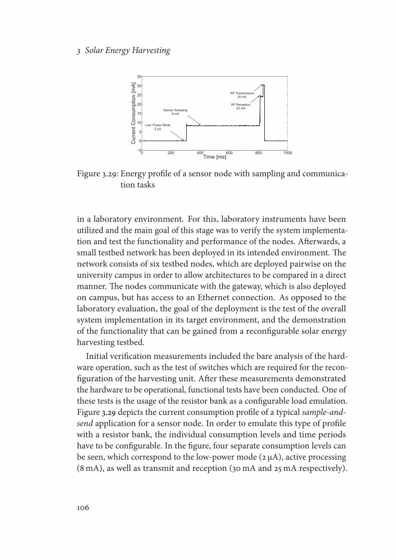
3 Solar Energy Harvesting
0 200 400 600 800 1000−5
0
5
10
15
20
25
30
35
Time [ms]
Cur
rent
Con
sum
ptio
n [m
A]
Low−Power Mode2 µA
Sensor Sampling8 mA
RF Transmission30 mA
RF Reception25 mA
Figure 3.29: Energy profile of a sensor node with sampling and communica-tion tasks
in a laboratory environment. For this, laboratory instruments have beenutilized and the main goal of this stage was to verify the system implementa-tion and test the functionality and performance of the nodes. Afterwards, asmall testbed network has been deployed in its intended environment. Thenetwork consists of six testbed nodes, which are deployed pairwise on theuniversity campus in order to allow architectures to be compared in a directmanner. The nodes communicate with the gateway, which is also deployedon campus, but has access to an Ethernet connection. As opposed to thelaboratory evaluation, the goal of the deployment is the test of the overallsystem implementation in its target environment, and the demonstrationof the functionality that can be gained from a reconfigurable solar energyharvesting testbed.Initial verification measurements included the bare analysis of the hard-
ware operation, such as the test of switches which are required for the recon-figuration of the harvesting unit. After these measurements demonstratedthe hardware to be operational, functional tests have been conducted. One ofthese tests is the usage of the resistor bank as a configurable load emulation.Figure 3.29 depicts the current consumption profile of a typical sample-and-send application for a sensor node. In order to emulate this type of profilewith a resistor bank, the individual consumption levels and time periodshave to be configurable. In the figure, four separate consumption levels canbe seen, which correspond to the low-power mode (2 μA), active processing(8mA), as well as transmit and reception (30mA and 25mA respectively).
106

3.4 Solar Energy Harvesting Testbed
0 100 200 300 400 500 600 700 800 900 10000
10
20
30
Time [Samples]
Cur
rent
Con
sum
ptio
n [m
A] Configured
Measured
Figure 3.30: Comparison of ideal and measured load emulation for the con-figurable load profiles on testbed nodes
Figure 3.30 shows that these values can be emulated by a resistor network ina simple manner and with relatively high accuracy. For the implementationresistors with a tolerance of 1 % have been used, which explains the increasingerror with increasing current emulation. As this method of a load emula-tion only requires a combination of resistor and transistor for each currentlevel to be emulated, increasing the load states is simple and inexpensive.Furthermore, time periods can be easily adjusted by utilizing standard timermodules, which allows for high resolution current profiles to be created. Thetime periods, in our implementation, can be defined with a resolution of62.5 μs.
Additionally, the consumption profile of the monitoring and control func-tion is of interest, as the system should operate reliably over a long periodof time without having access to a grid-based power supply. The node’s con-sumption profile, thus, defines how the back-channel power supply shouldbe dimensioned. Figure 3.31 shows the profile of an exemplar scenario. Thepresented scenario is that of the master node, which can be deduced fromthe two communication periods (i.e., one with the database and one with theother testbed nodes). Communication, in this implementation, occurs in afive minute interval, which is a trade-off between data resolution and powerconsumption of the back-channel node. The load emulation period, however,does not have to follow the same interval, which is illustrated in this scenario.Instead, the controller awakes four times per period and performs its controland monitoring task. The number of these sampling activities is not fixed
107

3 Solar Energy Harvesting
0 60 120 180 240 3000
10
20
30
40
50
60
70
Time [seconds]
Cur
rent
Con
sum
ptio
n [m
A]
Sampling11 mA, 70 ms Sleep
40 µA
Communication with Database62 mA, 100 ms
Communication with Network62 mA, 40 ms
Figure 3.31: Energy profile of a testbed node in operation. For the supply ofthe required energy, a power source, separate from the energyharvester under test, is utilized.
and can be adjusted on a per node basis within the harvester configuration.In addition, it can be defined as to how many of these samples the load peaksshould be applied to the architecture under test.
Finally, Figure 3.32 depicts exemplar output results of the deployed energyharvesting testbed. The results demonstrate how the testbed can supportthe analysis of location- and configuration-dependent performance of theharvesting architectures. Figure 3.32a, for example, shows a subset of thecomparison results, which have been obtained from different locations. Dur-ing the measurement, the same configurations have been applied to twoseparate nodes. One of these nodes has a southward orientation, while theother node is directed towards the north. The obtained measurements of thestate of charge illustrate this difference by means of the length of the dailycharge periods. Figures 3.32b and 3.32c, on the other hand, contain data fordifferent testbed configurations at the same node location. The difference ofthe architectural behavior for varying DLC capacities is depicted in Figure3.32b, whereas Figure 3.32c shows the influence of the load condition on thestate of charge in the same harvesting architecture.
108

3.4 Solar Energy Harvesting Testbed
0.5
1
1.5
2
2.5
Term
inal
Vol
tage
[V]
07/03
12:00
08/03
00:00
08/03
12:00
09/03
00:00
09/03
12:00
10/03
00:00
10/03
12:00
11/03
00:00
Southwards orientedNorthwards oriented
(a)
0.5
1
1.5
2
2.5
Term
inal
Vol
tage
[V]
11/03
00:00
12/03
00:00
13/03
00:00
14/03
00:00
15/03
00:00
16/03
00:00
1F DLC22F DLC
(b)
2
2.1
2.2
2.3
2.4
2.5
Term
inal
Vol
tage
[V]
28/03
12:00
29/03
00:00
29/03
12:00
30/03
00:00
10uA Avg. Load100uA Avg. Load
(c)
Figure 3.32: Exemplar output results of the solar energy harvesting testbed.The results show influence of (a) different node orientation, (b)different storage capacity, and (c) different load profile
109


4 Usability
Usability has been an active field of research, particularly, in the field ofwebsite and user interface design. Its main target is to reach a desired goal inan easier manner, such as finding a certain piece of information on a webpage. In order to quantify usability, five attributes have been defined [67],which are Learnability, Efficiency, Memorability, Errors and Satisfaction.
Learnability describes how easy it is for a new user to accomplish a task.Once the tool has been learned, efficiency defines how quickly a desiredtask can be performed. Memorability indicates how easy it is for a user toremember how to use the design, when it has been used previously. Errorsinclude how likely it is for the user to make a mistake, how severe thesemistakes are, and how simple it is to solve them. Finally, satisfaction describeshow satisfied a user is with the usage of the tool and the method to reach theintended goal.
As usability is a non-functional requirement of a design, it typically cannotbe measured directly. A typical evaluation method is the involvement of testusers, who represent the target user group and, thus, can provide qualitativefeedback. The integration of usability aspects should only have a minorimpact on the performance of the system. Trade-offs, however, are oftenrequired to be made. Nonetheless, the final system will only be useful if abalance is found. This usually means that a system, which can perform adesired task, but which a user does not know how to use it, is as useless asa system that is easy to be used, but does not match the user’s performancerequirements.
4.1 Usability inWireless Sensor Networks
In Wireless Sensor Networks, usability can be addressed with regards totwo distinct user groups, namely the system developer and the end user.
111

4 Usability
Particularly, in the environmental monitoring domain, but also in manyother application areas of WSNs, these user groups pose vastly different re-quirements in relation to the interface to be provided and, thus, the usabilityrequirements to be fulfilled. While for the development, parameters suchas the ease of programmability and debugging methods are of major inter-est, for the end users the concealment of complexity becomes of particularimportance. These factors can be addressed both on hardware and softwarelevel in the system design.Existing work towards the improvement of usability in Wireless Sensor
Networks has mainly focused on the software development aspect. This hasled to solutions that attempt to simplify application development, rangingfrom node languages [68–70] and operating systems [71, 72] to abstract lan-guage constructs that address the network as a whole [73–75]. Furthermore,the majority of these solutions are addressed towards system experts, thatmeans users who have a considerable understanding of the underlying sys-tem to be used. While this requirement is typically met in system researchapplications, in which systems are operated by their developers in order toconduct a proof of concept, in the long run WSNs are required to be operatedby their intended user group, who typically do not possess the currentlyrequired system skills.As a result, usability must be addressed for both user groups separately.
The remainder of this chapter will do so, and present usability considerationsand resulting design decisions for both groups, respectively. Furthermore, itwill be demonstrated that usability in sensor networks must be addressed forboth the hardware and software.
4.2 Usability for Developers
As has been indicated previously, the main goal for usability with respect todevelopment is the ease of programmability and debugging. This means, adeveloper should have interfaces in order to implement new applications oralgorithms in a quick and effective manner. Although this interface shouldlimit the chance ofmaking amistake during the implementation, additionally,debug interfaces should be available, which enable the user to efficiently testhis/her implementation and locate mistakes that have been made.
112

4.2 Usability for Developers
While Wireless Sensor Networks can, to some extent, profit from previousefforts in conventional computer systems – particularly with regards to pro-gramming methods – the resource limitation of the sensor nodes that aretypically used, restricts the methods that can be implemented in an effectivemanner. Furthermore, WSNs face challenges that complicate their operation,such as the deployment in remote and harsh environments. These conditionsmake proper debug interfaces a desired system attribute. Such interfaces,however, require time and energy and, thus, reduce the performance or thelifetime of the implemented system.In the following, two approaches for the improvement of usability for
system development will be presented. The major goal for both approacheshas been the maintenance of high performance, despite an increase in us-ability. Section 4.2.1 contains the presentation of a systematic programmingmethod based on Hierarchical Finite State Machines (HFSMs). The targetgroup for this programming method are system experts, who typically pos-sess the knowledge of describing systems and their behavior in the form ofFSMs. Thus, a translation from application description and its implementa-tion becomes easier, which reduces the risk of erroneous implementations.In Section 4.2.2, usability considerations for sensor node hardware platformswill be presented. These considerations are based on the typical constraintsin the environmental monitoring domain. The implementation of such con-siderations is demonstrated on the SENTIO-em hardware platform design(see also Section 2.4).
4.2.1 Programming with Hierarchical Finite State Machines
Microcontrollers are the typical implementation choice of the computationalmodule in wireless sensor nodes. Therefore, the development of the sourcecode, which defines the node’s behavior, typically occurs based on conven-tional embedded system development methods. This process is complicatedby the number of tasks a sensor node should perform – only a subset of whichare sensor sampling, processing, communication and network maintenance– and the desire of operating the node at low power consumption, whichresults in the usage of controllers with processing and memory limitations.As a consequence, programming methods for WSNs have been a topic ofinterest since the very beginning of sensor network research. This, in turn,
113
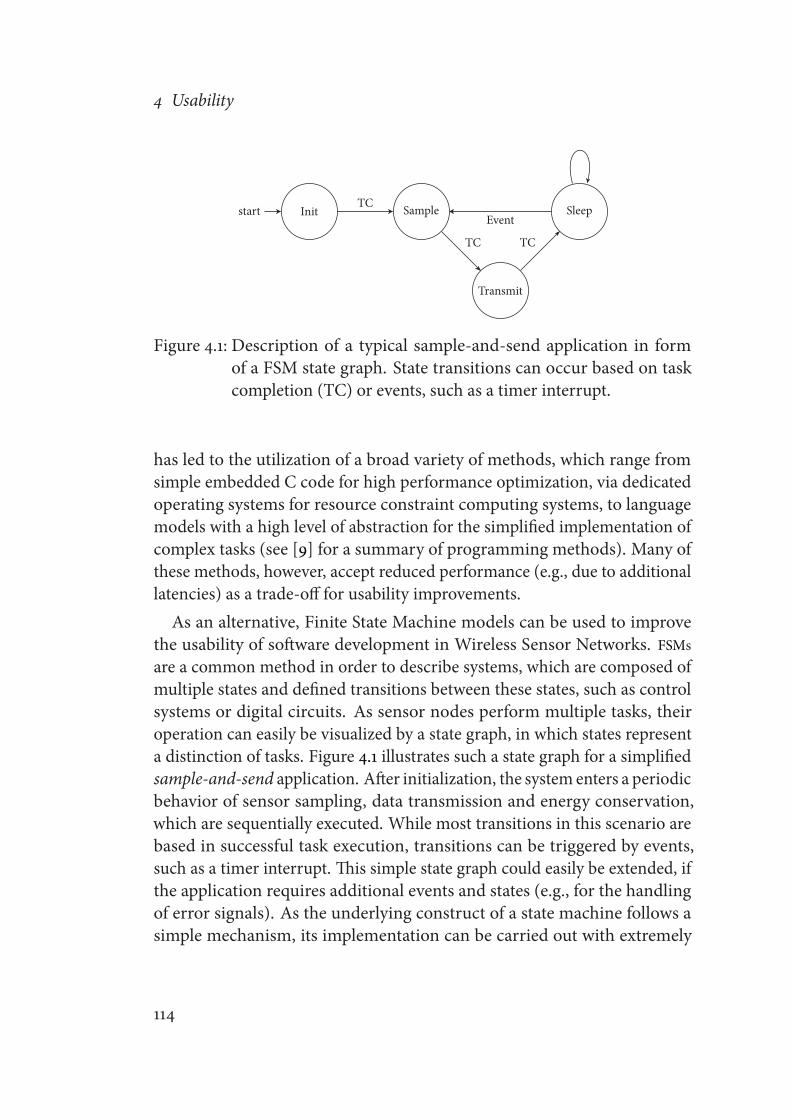
4 Usability
Initstart Sample
Transmit
SleepTC
TC TC
Event
Figure 4.1: Description of a typical sample-and-send application in formof a FSM state graph. State transitions can occur based on taskcompletion (TC) or events, such as a timer interrupt.
has led to the utilization of a broad variety of methods, which range fromsimple embedded C code for high performance optimization, via dedicatedoperating systems for resource constraint computing systems, to languagemodels with a high level of abstraction for the simplified implementation ofcomplex tasks (see [9] for a summary of programming methods). Many ofthese methods, however, accept reduced performance (e.g., due to additionallatencies) as a trade-off for usability improvements.As an alternative, Finite State Machine models can be used to improve
the usability of software development in Wireless Sensor Networks. FSMsare a common method in order to describe systems, which are composed ofmultiple states and defined transitions between these states, such as controlsystems or digital circuits. As sensor nodes perform multiple tasks, theiroperation can easily be visualized by a state graph, in which states representa distinction of tasks. Figure 4.1 illustrates such a state graph for a simplifiedsample-and-send application. After initialization, the system enters a periodicbehavior of sensor sampling, data transmission and energy conservation,which are sequentially executed. While most transitions in this scenario arebased in successful task execution, transitions can be triggered by events,such as a timer interrupt. This simple state graph could easily be extended, ifthe application requires additional events and states (e.g., for the handlingof error signals). As the underlying construct of a state machine follows asimple mechanism, its implementation can be carried out with extremely
114

4.2 Usability for Developers
low overhead.Programming methods can be evaluated based on a set of qualitative
parameters, including readability, modularity, reliability and efficiency. Theapplication of Finite State Machines as a programming method for sensornetworks can improve the software development with regards to several ofthese aspects. Because of the separation of the overall application architectureand the individual state implementation, readability is improved. Moreover,the number of states and the code length and structure within each state canalso increase readability. The same architectural properties make FSMs highlymodular. Existing states, as well as complete state machines, can easily bereused in multiple applications. As FSMs are a highly systematic manner ofdescribing a system, thismethod also has a positive influence on the reliabilityof the implemented code. Implementing a defined state transition for everypossible event, for example, allows for the application to end up in invalidsystem states which are to be avoided. Finally, these improvements can beachieved with low overhead, which results in an efficient code to be generatedfrom this programming method.While FSMs allow for applications to be split into smaller modules (i.e.,
states) and, thus, improve a number of factors in software development,a frequently mentioned disadvantage is the readability of a complex stategraph. As the number of states and transitions in a system increases, it canbe difficult to maintain an overview of the complete system structure. Thistypically leads to a trade-off between the number of states and transitions inthe system, and the code complexity of each state. Hierarchical Finite StateMachines can provide a solution in these cases by allowing multiple stategraphs to be composed, which are linked with each other. In Figure 4.1, forexample, the transmit-state could contain a separate FSM, which handles amore complex communication protocol. In this manner, a simple state graphis maintained on the top level, but complex states can be broken down intosubmodules for improved readability and maintainability.In order for the programming method to be tested, an HFSM framework
has been implemented for the SENTIO-em sensor node platform. Porta-bility of the implementation is maintained due to a layered architecture asdepicted in Figure 4.2. The architecture is based on an Hardware Abstrac-tion Layer (HAL), which allows for the code to be easily adjusted to otherhardware platforms. This layer contains the abstraction of the individual
115

4 Usability
Application Layer
Support Layer
Sub-FSM ATop-level FSM
Hardware Abstraction Layer
Radio Sensor A ISRUART
SharedMemoryADC Top A
Sensor BI2C
DriverInterface FSM Support
Figure 4.2: Layered architecture of the HFSM framework implementation forwireless sensor networks. Functions are separated by hardwareabstraction, state machine support, and the application.
driver modules and their functionalities and feeds into an unified driverinterface, which is part of the support layer. The driver interface allows forindividual modules to be selected for their usage in any given applicationcode. In addition, the support layer includes the actual FSM handling system,which evaluates the state graph and implements the defined state executionsand transitions. In order to keep the overhead of the handling system ata minimum, it uses an array of pointers to functions, which contains theaddresses of the individual state handlers, that means the functions in whichthe state contents are defined. The transitions between states in the applica-tion are, thus, only an index manipulation of an array, which results in fastexecution times and low processing overhead. For multiple state machinesbeing able to share event resources, which are typically the interrupt sourcesof the underlying hardware architecture, the Interrupt Service Routines (ISRs)have also to be shared. As common MCUs typically provide only a single ISRfor a given interrupt source, the sharing of this resource has to be manuallyintegrated. This has been achieved by a similar architecture to that of thestate transitioning. In the case of a HFSM utilization, each state machine inthe application is assigned a unique application ID. The ISRs are called froman array of pointers to functions, wherein each entry corresponds to one ofthe application IDs. In case an interrupt is triggered, the handling system
116

4.2 Usability for Developers
State valid?
true
Enter sleep-mode
Return to top-level
false Stay active?
Interrupt
Wake MCU & Call Interrupt Handler Call State-Handler
Start FSM
Continue operation?
true
false
false
true
Figure 4.3: Program flow of the executions of state transitions in the HFSMframework implementation.
will forward the event by pointing to the ISR defined in the array field of therespective application ID.While the support layer and the HAL are frameworkinternal, which means that they are typically not edited by the applicationdeveloper, the application layer provides an interface to the developer thatallows for the applications to be adjusted. This layer contains the code thatdefines the individual states, events and their relationships (i.e., the stategraph). In order to maintain integrity, the complete framework is developedin C++, which allows for invalid function calls to be avoided. Moreover,access between different function layers can be easily established by usingclass inheritance.Figure 4.3 provides an overview of the program flow in a typical HFSM
application. As low energy consumption is a critical component in sensornetwork applications, particularly in the environmental monitoring domain,the usage of low power modes has been integrated directly in the FSM frame-work. The developer, thus, has the choice of executing the next state in thestate graph directly, or entering an energy conserving low power mode whilewaiting for the event that will trigger the execution of the next state.
While the qualitative improvements of the implementation are difficultto measure, a quantitative evaluation of code efficiency has been performed
117
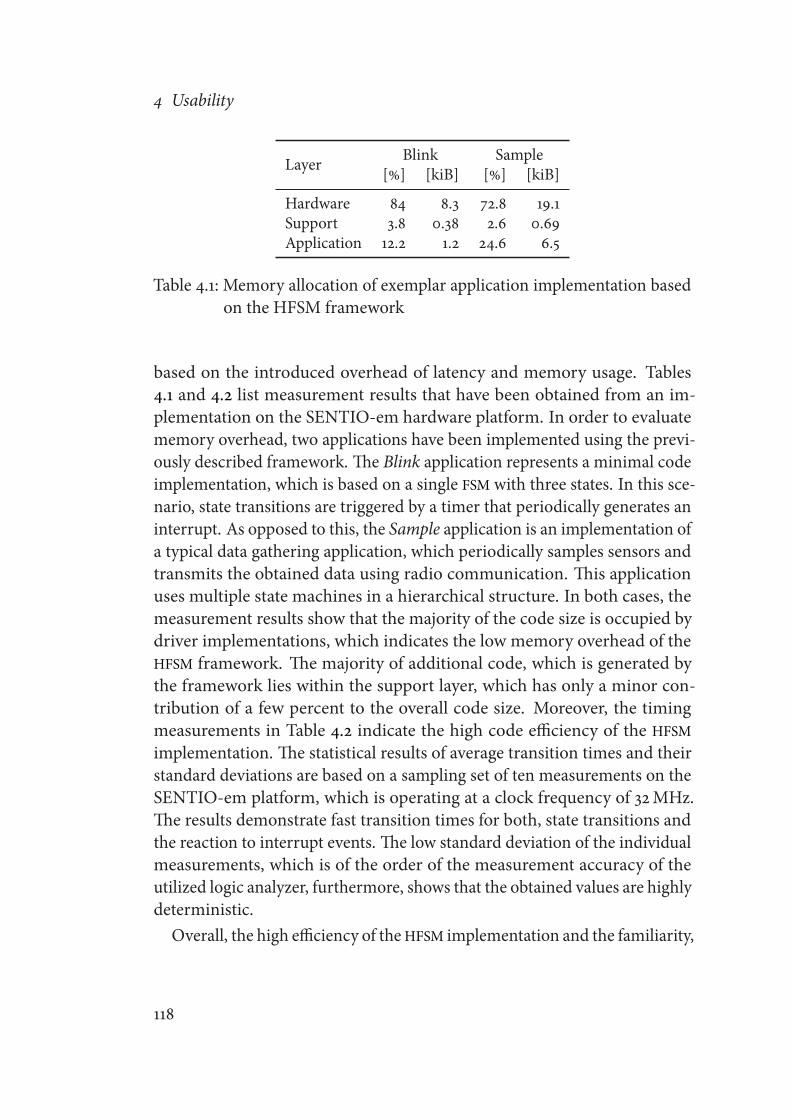
4 Usability
Layer Blink Sample[%] [kiB] [%] [kiB]
Hardware 84 8.3 72.8 19.1Support 3.8 0.38 2.6 0.69Application 12.2 1.2 24.6 6.5
Table 4.1: Memory allocation of exemplar application implementation basedon the HFSM framework
based on the introduced overhead of latency and memory usage. Tables4.1 and 4.2 list measurement results that have been obtained from an im-plementation on the SENTIO-em hardware platform. In order to evaluatememory overhead, two applications have been implemented using the previ-ously described framework. The Blink application represents a minimal codeimplementation, which is based on a single FSM with three states. In this sce-nario, state transitions are triggered by a timer that periodically generates aninterrupt. As opposed to this, the Sample application is an implementation ofa typical data gathering application, which periodically samples sensors andtransmits the obtained data using radio communication. This applicationuses multiple state machines in a hierarchical structure. In both cases, themeasurement results show that the majority of the code size is occupied bydriver implementations, which indicates the low memory overhead of theHFSM framework. The majority of additional code, which is generated bythe framework lies within the support layer, which has only a minor con-tribution of a few percent to the overall code size. Moreover, the timingmeasurements in Table 4.2 indicate the high code efficiency of the HFSMimplementation. The statistical results of average transition times and theirstandard deviations are based on a sampling set of ten measurements on theSENTIO-em platform, which is operating at a clock frequency of 32MHz.The results demonstrate fast transition times for both, state transitions andthe reaction to interrupt events. The low standard deviation of the individualmeasurements, which is of the order of the measurement accuracy of theutilized logic analyzer, furthermore, shows that the obtained values are highlydeterministic.
Overall, the high efficiency of the HFSM implementation and the familiarity,
118

4.2 Usability for Developers
Transition Condition AVG [μs] STD [μs]
Statedirect 1.56 0.004sleep (clock on) 3.8 0.007sleep (clock off) 6.77 0.007
Interrupt Enter ISR 0.77 0.007Enter Handler 1.74 0.007
Table 4.2: Measurement results of the latencies for state-to-state transitionsand interrupt handling
which has been generated by utilizing a programmingmethod for developers,who are comfortable with system descriptions in the form of Finite StateMachines, has the ability to improve the usability of software developmentfor technically experienced users.
4.2.2 Usability Considerations for Sensor Nodes
Although software considerations can support the implementation of ap-plication development, such as the programming method presented in theprevious section, an evaluation of the implemented software is required toverify its correct operation. Particularly in the development process, this canrequire evaluation measurements to be conducted and the localization ofimplementation mistakes. While software features, such as the utilizationof log files and additional debug outputs, can support this process, thesefunctionalities typically are associated with a cost in the form of softwareoverhead and additional resource usage. This, in turn, can change the actualapplication behavior or lead to an undesired overhead once the verificationprocess is completed. Hardware considerations on the sensor node platformcan support the development process by providing features that simplify suchevaluation measurements and, thus, improve the platform usability duringthe development period. At the same time, however, hardware overheadshould be maintained at a minimum in order for the platform to agree withthe desired cost and size constraints, which is of particular importance inapplications in which the number of sensor nodes can be large (e.g., in theenvironmental monitoring domain).
119

4 Usability
Initially, sensor node platforms have been envisioned to be of minimalsize in order to cover a large terrain at high density [76]. While the de-velopment of such miniaturized platforms continues [77], the majority ofexperimental research in WSNs is performed on sensor nodes of larger size,typically referred to as motes, which simplifies the development process dueto the possibility to integrate additional resources and provide easier accessin relation to those signals to be measured. Different concepts have beentested in order to combine the development support with the desired systemproperties, commonly agreed upon in the research community. The Telosmote [25], for example, can be connected to the development system (i.e.,typically a personal computer) in a simple manner, as it provides an interfacesimilar to that of a USB pen drive. While this has a positive impact on theplatform’s usability during laboratory operation, this feature does not supportthe deployment and, thus, experiments outside of the laboratory environ-ment. On the contrary, this form-factor might actually hinder the physicalenclosure and, thus, complicate deployment evaluations. Similar issues havebeen encountered on the waspmote platform, which has been used in theSAQnet case study (see Section 1.3). While the concept of sensor boardsallows for the platform to be prepared for specific application scenarios andsensors can easily be plugged into these boards in the laboratory, preparingthe nodes for outdoor deployment becomes difficult as sensor connectionshave to be extended. As a result, deployment becomes a tedious process,which has been acknowledged within the community [13].
In the design and implementation of the SENTIO-em sensor node plat-form, usability considerations with respect to both development and deploy-ment have been taken into account. The deployment considerations are ofparticular importance for the development of environmental monitoringwireless sensor networks, because evaluation tests in the targeted applicationenvironment are common. A key factor in the design of SENTIO-em arethe division of laboratory and deployment functionalities. While additionalresources are desirable during the development phase of a system, theseresources increase the size and cost of the node unnecessarily if they donot perform any contribution to the system operation after the deployment.Particularly in the environmental monitoring domain, in which outdooroperation might be performed for prolonged periods of time, these unusedresources are undesirable. A typical example of such resources is the USB
120

4.2 Usability for Developers
SENTIO-emLaboratory Dock
SENTIO-emCore Platform
Figure 4.4: Picture of the SENTIO-em platform implementation. The coreplatform is mounted on its dock solution for laboratory develop-ment.
interface. This interface is commonplace on many modern sensor node de-signs, as it allows for the node to be programmed via a serial bootloader, andfor debug messages to be sent to a computer terminal. During deployment,however, a USB interface does not provide any useful functionality and, thus,only results in wasted circuit space and additional node cost. Similar argu-ments can be brought forward for other modules, especially in relation touser interfaces, which only provide useful functionality during development.On the SENTIO-em platform, these functionalities have been separated fromthose which are required for the actual node tasks. As a result, a laboratorydocking solution has been created, which allows for extra development mod-ules to be provided during laboratory work, whereas the actual sensor nodeonly includes resources for its task execution in the field. Figure 4.4 depictsthis separation in the SENTIO-em implementation.While extension is a typically utilized concept in the design of wireless
sensor nodes, on SENTIO-em, extension interfaces have been grouped ac-cording to the modules that are attached. Sensors are a typical module to beseparated from the main sensor node, as the selection of sensors is highlyapplication specific. Moreover, extended power supply units, such as forthe utilization of ambient energy sources, require a power interface withincreased complexity to be provided. As a result, signals and communicationinterfaces are available in order to control and monitor the power supply unit,
121

4 Usability
as opposed to the bare reception of energy. An additional debug interfaceis used, mainly, in order to enable the previously mentioned separation ofdevelopment and deployment resources. For the implementation of theseinterfaces, standard 2mm connectors have been used, which allow for board-to-board and wire-to-board connections to be established in a mechanicallyrobust manner.
Although wireless communication is an essential part of a sensor node, ina later revision of SENTIO-em, this module has been removed, but is insteadconnected in a plug-in manner. This separation choice has multiple reasons,which affect the usability of the platform. Firstly, individual applications canhave varying requirements on communication properties, such as carrier fre-quency and data rates. Moreover, a vast amount of communication protocolsare available, which offer their respective advantages in specific applicationareas. Finally, the evaluation of a new radio transceiver is simplified, as thedevelopment is restricted to the communication module, as opposed to theimplementation or adjustment of a complete sensor node. For themechanicalconnection, the XBee form-factor has been chosen. The XBee series of radiotransceivers are commercially available and have gained particular interestin hobby electronics, due to their simple usage. Selecting its form-factorfor SENTIO-em allows for the rapid prototyping with a set of wireless com-munication standards and transceiver properties to be performed. Radiotransceiver options, which have been used on the SENTIO-em platform,include low-frequency transceivers, IEEE 802.15.4 and IEEE 802.11 modules.
Considerations on the form-factor of a sensor node platform have typicallybeen restricted to small physical size. In the environmental monitoringdomain, however, the node size is, in the majority of cases, not a primaryrestriction. However, it is the case that easy deployability is typically ofhigher importance. As was previously mentioned, the deployment processin environmental monitoring applications can be rather tedious. A reason,amongst others, is the necessity of preparing the sensor node for outdoordeployment, which includes the enclosing of the electronic system. An optionin order to improve this process is the design of a customized enclosure.This, however, is a costly solution, which is typically not feasible within thescope of most research projects. For SENTIO-em we have chosen the inverseprocedure and designed the node with a customized form-factor for a specificphysical enclosure. While this requires minor adjustments to the Printed
122

4.3 Usability for End Users
Circuit Board (PCB) size, this solution comes at virtually no cost. SENTIO-em has been designed with a form-factor in compliance with a Hammond1591T enclosure1, which allows screwless mounting of PCBs in a number ofmolded card guides.A great number of experimental projects in WSNs have documented the
contradiction of debug possibilities after deployment and the resource limita-tion of typical sensor nodes. One reason is the uncertainty of the necessity fordebugging at the time of system deployment. In the case for which debuggingis required, but no method is implemented, errors are likely to remain unde-tected, which typically results in the return of the system to the laboratory.On the other hand, if debugging methods have been provided, but are notrequired, the system operation might be restricted, because resources arewasted for a function that is unnecessary. A desirable alternative is the optionto enable debug options, if required, while disabling them otherwise. This,however, commonly requires opening up the enclosure of a node, which ishighly undesirable in outdoor deployments, particularly after nodes havebeen weatherproofed. In order to prepare SENTIO-em for this scenario,two magnetic switches have been integrated, which allow interactions tobe performed with an enclosed node. The switches have been placed withthe largest possible distance between each other in order to avoid accidentaltriggering of the wrong switch. While one of the switches lies in the node’spower line and, thus, allows for the node to be remotely disabled or reset,the second switch can trigger a user-defined interrupt, which might be usedto enable or disable certain node functionalities without the requirement toopen the node’s enclosure.
4.3 Usability for End Users
As opposed to the systemdeveloper, who has a profound understanding of theunderlying system architecture of aWSN, the typical end user of such a systemhas experience with the domain the system should be used in, rather thanthe system itself. Moreover, in the environmental monitoring domain, it ishighly uncommon for end users to possess skills related to the programmingof computer systems, let alone embedded systems, which are the primary
1http://www.hammondmfg.com/dwg2a.htm
123

4 Usability
method of interacting with sensor nodes at the present time. Nonetheless,the requirement of hiring a system expert in order to operate a WSN as ameasurement system is not feasible and limits the real-world applicability ofsuch systems.While there has been a great amount of research on the simplification of
programming methods with respect to WSNs (see Section 4.2.1), the interac-tion methods that do not use any form of programming language are strictlylimited. Solutions, that come closest to this requirement, are referencedin [73, 78]. While [78] presents a method of using spreadsheets in order toconfigure WSNs, [73] uses an interface similar to database abstractions. Inboth cases, however, an evaluation of the usability of the respective methodwith regards to the targeted end user is missing.
4.3.1 Concealing Node Programming Complexity
Concealing the technological complexity of a system is not limited to WSNs.Personal computers, for example, have very similar issues when being op-erated by an inexperienced user. Much effort, however, has been spent inmaking relatively complex tasks appear easy to the end user, by automatingrequired tasks and by performing them in the background. Such tasks canbe the installation of new software or the operation of hardware peripheralsin a plug-and-play fashion. Similar methods can be utilized in order to makeWSNs more accessible to non-technical users.
While different concepts can be utilized, in this study, a wizard-basedconfiguration of sensor nodes has been selected. This choice has multiplereasons, including the user familiarity of the concept from software instal-lations, the guided flow from the start to the end of the task to be executed,the step-wise execution of the task, as well as the possibility to maintain asimilar process as used when collaborating with a system expert. Figure 4.5depicts the conventional system design process, in which a domain scientistprovides system specifications to a system expert, who, in turn, will imple-ment the system to conform to the application requirements. Figure 4.6illustrates how the conventional process can be adjusted in order to removethe system expert by utilizing a wizard-based specification method. Assum-ing that the domain expert has access to a sensor node, the specificationshave to be translated into a firmware, which can be uploaded to the node,
124
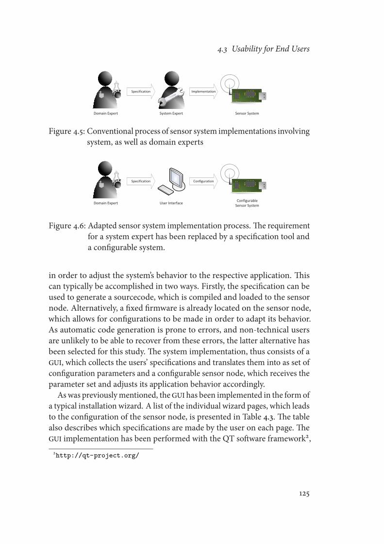
4.3 Usability for End Users
Domain Expert System Expert Sensor System
Specification Implementation
Figure 4.5: Conventional process of sensor system implementations involvingsystem, as well as domain experts
Domain Expert User Interface Configurable Sensor System
Specification Configuration
Figure 4.6: Adapted sensor system implementation process. The requirementfor a system expert has been replaced by a specification tool anda configurable system.
in order to adjust the system’s behavior to the respective application. Thiscan typically be accomplished in two ways. Firstly, the specification can beused to generate a sourcecode, which is compiled and loaded to the sensornode. Alternatively, a fixed firmware is already located on the sensor node,which allows for configurations to be made in order to adapt its behavior.As automatic code generation is prone to errors, and non-technical usersare unlikely to be able to recover from these errors, the latter alternative hasbeen selected for this study. The system implementation, thus consists of aGUI, which collects the users’ specifications and translates them into as set ofconfiguration parameters and a configurable sensor node, which receives theparameter set and adjusts its application behavior accordingly.
Aswas previouslymentioned, the GUI has been implemented in the formofa typical installation wizard. A list of the individual wizard pages, which leadsto the configuration of the sensor node, is presented in Table 4.3. The tablealso describes which specifications are made by the user on each page. TheGUI implementation has been performed with the QT software framework2,2http://qt-project.org/
125

4 Usability
Wizard Page Specification Parameters
Node/Network Node name and network affiliationSensing Sensor selection and sample rate
Communication Time- or event-driven communicationSensor threshold (only event-driven)
Processing/Storage Processing type and sample setStorage option (all or transmitted samples)
Verification Clear text node behavior listingLifetime Lifetime estimate and adjustment optionsConfiguration Configuration save and upload option
Table 4.3: Page overview of the specification wizard with the respective speci-fication parameters to be defined.
which provides access to a number of libraries for user interface developmentand a broad user community. In the implementation, special considerationhas been paid to the usage of natural language, as opposed to technical terms.The intention was to allow the users to answer simple questions about theirintendedmeasurement application, in which the answers could be binary (i.e.,yes or no), a selection from a provided list, or a numeric specification, such asrequired for sample periods. Combinations of answers, which are technicallyimpossible or do not make sense, are avoided if possible. In general, specialattention has been paid to avoid entries, which result in erroneous nodebehavior, as technically unexperienced users are unlikely to localize andrevert such implementations.
In order to create a configurable sensor node, the firmware which runs onthe node has been parametrized. This means that its behavior is altered basedon the configuration parameters, which are received from the specificationtool. As a result, unused functions are disabled and numeric configurations,such as sensor sample rates, are adjusted. In order to allow for the currentconfiguration to be maintained, even after a reset condition (e.g., when thenode has been disabled for a period of time), the received configurationparameters are stored in a non-volatile memory. The parametrized firmware
126

4.3 Usability for End Users
Initialization
Load Existing Configuration
Configuration Update
Sleep
Sensor Sampling
ProcessingCommunication Storage
Periodic
Figure 4.7: State-graph of the configurable sensor node firmware. The config-uration update state can be reached by an event from any state inthe graph.
has been implemented on the SENTIO-em platform, and is based on theHFSM programming model, which has been presented in Section 4.2.1. Asopposed to if-else or switch conditions, which would typically be used inorder to create a configurable firmware behavior, the utilization of an FSMbased firmware allows for configurations to be performed by altering thestate graph of the application. As the result is a single evaluation at the timeof parameter reception, runtime overhead is significantly reduced in compar-ison to continuous condition evaluations. An overview of the implementedfirmware is given in Figure 4.7. For the transmission of the configurationparameters from the specification wizard to the sensor node, a conventionalUSB interface has been utilized. The interface allows for the configurationsto be performed on any PC-class workstation, without further requirementon specialized hardware resources. Moreover, the physical connection ofthe interface enables the specification software to automatically detect com-patible sensor node devices. Based on the small number of configurationparameters to be transmitted, however, the interface can easily be switchedin order to perform configurations wirelessly. As multiple devices might be
127

4 Usability
Power Supply Selectionand USB Interface
Temperature and Humidity Sensor
SENTIO-em Node Platform
Figure 4.8: Implementation of the configurable sensor node design for theconduction of user evaluations.
in communication range, however, additional precautions must be met forthe correct device to be configured.
For the evaluation of the implemented system, the configurable firmwarewas loaded to an enclosed sensor node, which has been equipped with anUSB extension and example sensors (see Figure 4.8). This sensor node, incombination with the implemented specification tool, has been supplied toa number of test users. The group of test users was selected on a voluntarybasis and included users with limited programming skills, who represent thetargeted end user type, but also technically experienced personal, who couldprovide detailed comments on the implemented configuration method. Asthe scope of the evaluation did not allow for actual measurement problemsto be implemented, the users have been instructed with a set of measurementscenario descriptions. The scenarios have been developed in a role-play man-ner, which provided the user with his/her intentions and the measurementgoal to be performed. Detailed instructions regarding how to perform theimplementation of these measurement goals have been omitted purpose-fully. Afterwards, the users were asked to implement their measurement goalon the implemented system. During the implementation phase, no further
128
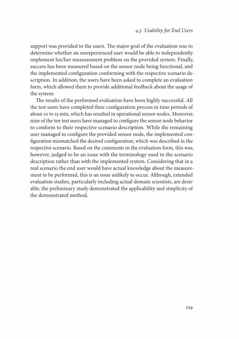
4.3 Usability for End Users
support was provided to the users. The major goal of the evaluation was todetermine whether an unexperienced user would be able to independentlyimplement his/her measurement problem on the provided system. Finally,success has been measured based on the sensor node being functional, andthe implemented configuration conforming with the respective scenario de-scription. In addition, the users have been asked to complete an evaluationform, which allowed them to provide additional feedback about the usage ofthe system.The results of the performed evaluation have been highly successful. All
the test users have completed their configuration process in time periods ofabout 10 to 15 min, which has resulted in operational sensor nodes. Moreover,nine of the ten test users have managed to configure the sensor node behaviorto conform to their respective scenario description. While the remaininguser managed to configure the provided sensor node, the implemented con-figuration mismatched the desired configuration, which was described in therespective scenario. Based on the comments in the evaluation form, this was,however, judged to be an issue with the terminology used in the scenariodescription rather than with the implemented system. Considering that in areal scenario the end user would have actual knowledge about the measure-ment to be performed, this is an issue unlikely to occur. Although, extendedevaluation studies, particularly including actual domain scientists, are desir-able, the preliminary study demonstrated the applicability and simplicity ofthe demonstrated method.
129


5 Discussion and Conclusions
Environmentalmonitoring can benefit greatly from the utilization ofWirelessSensor Networks, as its usage allows for measurements to be performedwith adjustable spatial and temporal distributions. Although the network iscomposed of individual sensor nodes, which are distributed in the site to bemonitored, the system typically can be operated from a single location byremotely accessing the network to be controlled. A number of applicationexamples and proof-of-concept studies have demonstrated these benefits in-situ. However, they have also uncovered technical challenges to be addressedin order for WSNs to become a feasible measurement solution in the domain.Among these challenges are the operational lifetime of the network and theusability of the system setup, which have been addressed on the system levelin this thesis.The lifetime of a WSN, which is tightly correlated with the lifetime of
the individual sensor nodes in the network, has been a concern since thebeginning of research in this domain. As a result, a great amount of workhas been conducted in order to prolong the lifetime of a node. Contributionsto this research have been made by the work, presented in this thesis, in twoseparate ways, namely the energy efficiency improvement of the sensor node’stask execution and the extension of available energy resources by utilizingambient energy sources.With respect to the energy efficiency, a wireless sensor node implemen-
tation has been presented, which is specifically designed for its applicationin low sample rate data gathering scenarios, which are commonplace in theenvironmental monitoring domain. The utilization of a modern controllerarchitecture and the separation of power domains for individual submodules,allowed for the node design to both increase the processing performanceand decrease the power consumption as compared to common referencenodes. Special attention has been paid to the reduction of quiescent currents,which will define the power consumption in low-power modes and, thus,
131

5 Discussion and Conclusions
define the overall energy consumption in low duty cycle applications. Inorder to achieve such low duty cycles, the active task periods are required tobe minimized. This involves, particularly, wireless communication tasks, asits contribution to the energy consumption can be considerable, because ofits relatively high power levels. A simple synchronization method has beenpresented, which allows for short communication periods to be achieved,due to the possibility of scheduling such tasks in a TDMA-like manner. Theutilizedmethod demonstrates synchronization accuracies of the order of tensto hundreds of μs, which allows for accurate time slots to be created, whilemaintaining a minimal overhead for the required synchronization. Although,a division exists within the research community between contention-freeand contention-based communication protocols, with contention-based pro-tocols being used in the majority of applications, contention-free protocolspossess multiple advantages in relation to data gathering applications. Themajor advantages of contention-based protocols are its low latency and thepossibility to adjust to a dynamic system behavior. These features, however,have only low value in typically static environmental measurement systemswith low requirements on latency. A limitation of time-scheduled protocolsis its restricted scalability, which, however, can be improved by utilizinghierarchical scheduling mechanisms. The optimized implementation andits respective performance evaluations of such a hierarchical method arecurrently being analyzed.
While the improvement of energy efficiency allows for the lifetime of sen-sor nodes to be extended, a limitation remains due to the restricted capacityof the energy source, which is commonly battery based. Particularly in out-door applications, solar energy harvesting has been an appropriate methodin order to virtually increase the energy capacity of a sensor node. The major-ity of such systems, however, have been demonstrated, based on secondarybatteries, which are inherently limited in their device lifetime. While thelarge capacity of batteries are required in certain applications, low powerapplications have been demonstrated with DLCs as their storage medium.Double Layer Capacitors can store only relatively small amounts of energy,but they have a high power density, which allows for their charge level to bequickly restored. Moreover, as energy is stored in the form of charge sepa-ration, as opposed to the chemical reactions that are occurring in batteries,the lifetime of DLCs are much higher. For the usage of DLCs in solar energy
132

harvesting architectures, however, regular irradiation is required in order tosupply the sensor node from a small capacity for prolonged periods of time.This has limited the application of these energy buffers to locations withhigh solar irradiation. Contributions from this thesis, have demonstratedthat it is feasible to utilize short-term energy buffers, such as DLCs, even atlocations with limited solar irradiation. A number of solar energy harvestingarchitectures have been implemented and analyzed in order to evaluate thesystem behavior. The major focus, in relation to this, has been the energyoverhead of the harvester itself, meaning the amount of energy it takes tooperate the harvester, which will define the irradiance level from which en-ergy can be harvested. As an alternative to DLCs, Thin-Film Batteries havebeen analyzed for usage in solar energy harvesting architectures. While TFBshave been demonstrated to be a feasible alternative in low power applications,their currently high internal resistance, in combination with a limitation toextremely small capacities, restricts the scalable utilization of these devices.As a result, the DLCs present a number of advantages in applications, forwhich size is not the primary limitation. Further analysis of the scalabilityof DLC based systems for sensor nodes with higher power consumption areunder consideration.A common dispute exists between researchers in the community as to
whether MPPT should be utilized in small-scale solar energy harvesting appli-cations, such as those implemented as sensor node power supplies. While theperformance improvement of MPPT, in general, is irrefutable, its operationaloverhead does not scale with the scaling harvesting system. As a result, theoverhead created by common MPPT techniques becomes considerable, whichresults in the utilization of simplified, less accurate, tracking methods. While,initially, MPPT has been avoided in the harvesting architectures, architectureswith a commercial harvesting circuit, which utilize MPPT, have been eval-uated. In comparison with previous architectures, which were optimizedfor low energy overhead, these architectures have demonstrated a reducedperformance in low irradiance situations. This result verified the initial ex-pectations, as most simplified MPPT methods utilize constant factoring of theopen-circuit voltage or short-circuit current, which is typically optimized forhigh irradiance levels.As experimental evaluations have proven to be valuable for the compari-
son of harvesting architectures, however, the work load, which is required
133
5 Discussion and Conclusions
for repetitive system deployments, is considerable, a novel approach for theevaluation of multiple architectures and configurations has been developed.The system is based on the ideas of remote configuration and monitoring,which is typically implemented in WSN testbeds. Such a solar energy harvest-ing testbed can, therefore, be used to conduct multiple experiments, whilethe system is deployed only once. The system design of the presented sys-tem uses a typical WSN architecture in order to send configuration packetsand collect measurement parameters. Each node, however, is extended bymeans of a harvesting module, which allows configurations to be made toits hardware. The testbed is operated via a user interface that allows forconfigurations to be created and assignments of configurations to individualtestbed nodes to be made. Moreover, the same interface can be used in orderto access the collected data for visualization or further analysis. The systemhas been implemented and tested in a proof-of-concept deployment of thesolar energy harvesting testbed. Evaluation results on the performance ofthe testbed nodes and exemplar output values from the testbed have beencollected, and they demonstrate how the solar energy harvesting can be usedin order to collect experimental results for the analysis and modeling of solarenergy harvesting architectures in a more efficient manner. A limitation tothe system is the requirement to have knowledge of the type of desirableconfigurations, as the configurable hardware has to be prepared accordingly.This limitation can be addressed by developing a unified interface, whichallows for modular harvesting modules to be implemented in the system in aplug-and-play fashion. While the control and monitoring architecture couldbe maintained, the actual harvesting circuitry would be exchangeable, whichallows for the experimental setup to be altered in order to integrate newharvesting methods to the testbed. An adjustment in this form is planned tobe developed for further improvement in relation to system flexibility.
Although experimental evaluations are important in order to understandand compare individual harvesting methods, their results can additionallycontribute to the development of accurate component and system models.Thesemodels, in turn, are important to accelerate the study of ambient energyharvesting, as well as their appropriate utilization in actual WSN applications.While ambient energy sources, such as solar irradiation, are not capacity lim-ited, a rate limitation applies which is based on diurnal, seasonal and spatialvariations. This means that systems with the same configuration will behave
134

differently if the system is deployed at a different time or location. Priorto network deployment, adjustments to the harvester configuration (e.g.,storage or panel size) or the energy profile of the node (e.g, by adjustmentto the sample rate) might be required in order to establish perpetual systemoperation. As an analogy, capacities in pure battery operated sensor nodesare selected dependent on load conditions and the desired system lifetime.While this typically occurs on an analytical basis for batteries, the complexityof irradiation patterns and the energy harvesting circuitry prohibits an ana-lytical method if solar energy harvesting is utilized. We have proposed themodeling of the energy harvesting architecture in order to simulate the stateof charge at any given point in time. Similarly, to the calculation of the batterylifetime, these estimations can be used in combination with load conditionsand irradiation parameters in order to determine the optimal configurationof the system to be used. The implementation of an exemplar harvestingarchitecture based on individual component models demonstrated the accu-racy of this modeling technique and their respective simulations. Difficultiesarise, however, due to the time consuming development of accurate systemmodels. Furthermore, in the case of the utilization of commercial ICs, thecreation of an accurate component model becomes tremendously difficult.The study of alternative modeling methods, which promise faster model de-velopment, has been initiated. In this respect, particularly, the application ofartificial neural networks appears to be promising, as a complete harvestingarchitecture can be modeled at one time, without the necessity of modelingeach individual component of the architecture. A loss in accuracy, however,is expected as a trade-off for model development time.In addition to the contributions to the improvement of sensor node life-
time, the usability of sensor nodes has been addressed in this thesis. Thishas been carried out for developers and end users separately, as each grouppresents their individual needs and skills. While developers typically requireinterfaces that allow for the development of new applications and algorithmsto be performed in an effective manner, end users require simplified in-terfaces, which enable them to configure an existing system towards theirapplication requirements. In order to increase the usability for the developers,who possess a technical understanding of the underlying system, a Hierar-chical Finite State Machine programming framework has been designedand implemented. The utilization of FSMs for the software development in
135

5 Discussion and Conclusions
sensor nodes allows for the development process to be carried out in a sys-tematic manner. Moreover, software can be easily split into smaller modules(i.e., states), which improves the readability and modularity of the generatedsource code. Evaluation results show that the implemented applications con-tain only limited overhead, both in timing and memory usage. The usabilityimprovements, which are gained from this programmingmethod, thus, comeat low cost. Although usability is only improved in cases of user familiaritywith FSMs, this is to be expected in the majority of cases, as system developersare typically computer scientists or engineers, who are commonly exposedto FSM description models.While improving the usability of programming methods can reduce the
amount of mistakes to be made, it cannot completely eliminate the necessityof verification measurements. The resource limitation of sensor nodes, whichis typically a result of size and cost restrictions, hinders these measurementsto be conducted in an effective manner. We proposed a number of simpleconsiderations to the design of wireless sensor nodes, which can improve theusability in evaluation scenarios. These considerations have been presentedbased on typical environmental monitoring requirements, and have beenimplemented in the design of the SENTIO-em node platform. The usage ofthe SENTIO-em platform in a number of outdoor experiments, has success-fully demonstrated the gained usability improvements of the implementedmodifications.Finally, end user accessibility to WSNs has been the focus of the investiga-
tions performed in this thesis. Although domain experts have been part ofthe development process in a number of environmental monitoring appli-cations, the systems, in these scenarios, have been operated by the systemdevelopers (i.e., system experts) rather than the designated end user (i.e.,the domain experts). As a result, the real-world applicability of WSNs as ameasurement instrument in the domain, is strictly limited. A method hasbeen presented, which allows for end users to modify the node behavioraccording to application requirements, without the necessity of a technicalunderstanding of the utilized system. The modifications are performed viaa GUI, which reproduces the method of software installations. The createdconfiguration parameters are used in a configurable firmware in order toalter the sensor node behavior. The feasibility of the configuration methodhas been evaluated by means of a number of test users, which demonstrated
136

the usability of the implemented system. Improvements are planned to beconducted in two ways. On the one hand, the hardware configuration hasto be simplified in order for users to equip the sensor node according totheir specific needs. This means, in the main, that users should be able toconnect the desired sensor modules to the node in a simple manner. Thedevelopment of a unified sensor interface, which allows for the sensor to bedetected and configured by the sensor node in an automatic fashion, appearsto be a feasible solution. Furthermore, extended usability tests are to beconducted, which involves actual domain experts and real-world applicationtasks. A more detailed evaluation, which could include the recording of theuser and the activity in the GUI, might support the optimization of the layoutand formulations in the design.In overall conclusion, the work that has been presented in this thesis,
contributed to node level improvements, which improve the real-world appli-cation of WSNs in measurement scenarios for the environmental monitoringdomain. While improvement opportunities remain, the presented method-ologies and implementations support the prolonged operational lifetimeand efficient system utilization. These are both required steps for WirelessSensor Networks in order to leave proof-of-concept evaluations and becomereal-world applicable measurement instruments.
137


Bibliography
[1] J. Artiola, I. Pepper, and M. Brusseau, Environmental Monitoring andCharacterization. Elsevier Academic Press, 2004.
[2] Proceedings of the Distributed Sensor Nets Workshop, (Carnegie MellonUniversity, Pittsburgh, Pennsylvania), 1978.
[3] J. Porter, P. Arzberger, H.-W. Braun, P. Bryant, S. Gage, T. Hansen,P. Hanson, C.-C. Lin, F.-P. Lin, T. Kratz, W. Michener, S. Shapiro, andT. Williams, “Wireless Sensor Networks for Ecology,” BioScience, vol. 55,no. 7, pp. 561–572, 2005.
[4] G. Barrenetxea, F. Ingelrest, G. Schaefer, M. Vetterli, O. Couach, andM. Parlange, “Sensorscope: Out-of-the-Box Environmental Monitor-ing,” in Proceedings of the 7th International Conference on InformationProcessing in Sensor Networks (IPSN), pp. 332–343, 2008.
[5] T.Wark,W.Hu, P. Corke, J. Hodge, A. Keto, B.Mackey, G. Foley, P. Sikka,and M. Brunig, “Springbrook: Challenges in Developing a Long-Term,Rainforest Wireless Sensor Network,” in Proceedings of the Fourth In-ternational Conference on Intelligent Sensors, Sensor Networks and In-formation Processing (ISSNIP), pp. 599–604, 2008.
[6] F. Ingelrest, G. Barrenetxea, G. Schaefer, M. Vetterli, O. Couach, andM. Parlange, “SensorScope: Application-Specific Sensor Network forEnvironmental Monitoring,” ACM Transactions on Sensor Networks,vol. 6, pp. 1–32, Feb. 2010.
[7] D. M. Doolin, “Wireless Sensors for Wildfire Monitoring,” in Proceed-ings of SPIE, vol. 5765, pp. 477–484, 2005.
139

Bibliography
[8] G. Werner-Allen, K. Lorincz, M. Ruiz, O. Marcillo, J. Johnson, J. Lees,and M. Welsh, “Deploying a Wireless Sensor Network on an ActiveVolcano,” IEEE Internet Computing, vol. 10, pp. 18–25, Mar. 2006.
[9] L. Mottola and G. P. Picco, “Programming Wireless Sensor Networks,”ACM Computing Surveys, vol. 43, pp. 1–51, Apr. 2011.
[10] T. Le Dinh, W. Hu, P. Sikka, P. Corke, L. Overs, and S. Brosnan, “DesignandDeployment of a Remote Robust SensorNetwork: Experiences froman Outdoor Water Quality Monitoring Network,” in Proceedings of the32nd IEEEConference on Local Computer Networks (LCN), pp. 799–806,2007.
[11] K. Martinez, R. Ong, and J. Hart, “Glacsweb: A Sensor Network forHostile Environments,” in Proceedings of the First Annual IEEE Com-munications Society Conference on Sensor and AdHoc Communicationsand Networks (SECON), pp. 81–87, 2004.
[12] L. Selavo, A. Wood, Q. Cao, T. Sookoor, H. Liu, A. Srinivasan, Y. Wu,W. Kang, J. Stankovic, D. Young, and Others, “Luster: Wireless SensorNetwork for Environmental Research,” in Proceedings of the 5th Inter-national Conference on Embedded Networked Sensor Systems (SenSys),pp. 103–116, 2007.
[13] E. Gaura, L. Girod, J. Brusey, M. Allen, and G. Challen, eds.,WirelessSensor Networks - Deployments and Design Framework. Springer, 2010.
[14] A. Mainwaring, D. Culler, J. Polastre, R. Szewczyk, and J. Anderson,“Wireless Sensor Networks for Habitat Monitoring,” in Proceedings ofthe 1st ACM International Workshop on Wireless Sensor Networks andApplications (WSNA), pp. 88–97, 2002.
[15] R. Szewczyk, A. Mainwaring, J. Polastre, J. Anderson, and D. Culler,“An Analysis of a Large Scale Habitat Monitoring Application,” in Pro-ceedings of the 2nd International Conference on Embedded NetworkedSensor Systems (SenSys), pp. 214–226, 2004.
140

Bibliography
[16] K. Martinez, P. Padhy, A. Elsaify, G. Zou, A. Riddoch, J. Hart, andH. Ong, “Deploying a Sensor Network in an Extreme Environment,”Sensor Networks, Ubiquitous and Trustworthy Computing, 2006.
[17] K. Martinez, J. K. Hart, and R. Ong, “Deploying a Wireless SensorNetwork in Iceland,” in Proceedings of the 3rd International Conferenceon GeoSensor Networks (GSN), pp. 131–137, 2009.
[18] K. Langendoen, A. Baggio, and O. Visser, “Murphy Loves Potatoes: Ex-periences from a Pilot Sensor Network Deployment in Precision Agri-culture,” in Proceedings of the 20th International Conference on Paralleland Distributed Processing (IPDPS), 2006.
[19] G. Werner-Allen, J. Johnson, M. Ruiz, J. Lees, and M. Welsh, “Monitor-ingVolcanic Eruptionswith aWireless SensorNetwork,” inProceeedingsof the Second EuropeanWorkshop onWireless Sensor Networks (EWSN),pp. 108–120, 2005.
[20] G. Tolle, D. Gay, W. Hong, J. Polastre, R. Szewczyk, D. Culler, N. Turner,K. Tu, S. Burgess, T. Dawson, and P. Buonadonna, “A Macroscope inthe Redwoods,” in Proceedings of the 3rd International Conference onEmbedded Networked Sensor Systems (SenSys), p. 51, 2005.
[21] W. Hu, N. Bulusu, C. T. Chou, S. Jha, A. Taylor, and V. N. Tran, “Designand Evaluation of a Hybrid Sensor Network for Cane Toad Monitoring,”ACM Transactions on Sensor Networks, vol. 5, pp. 4:1–4:28, Feb. 2009.
[22] I. Dietrich and F. Dressler, “On the Lifetime of Wireless Sensor Net-works,” ACM Transactions on Sensor Networks, vol. 5, pp. 1–39, Feb.2009.
[23] J. Hill and D. Culler, “Mica: A Wireless Platform for Deeply EmbeddedNetworks,” IEEE Micro, vol. 22, no. 6, pp. 12–24, 2002.
[24] P. Sikka, P. Corke, L. Overs, P. Valencia, and T. Wark, “Fleck - A Plat-form for Real-World Outdoor Sensor Networks,” in Proceedings of the3rd International Conference on Intelligent Sensors, SensorNetworks andInformation Processing (ISSNIP), pp. 709–714, 2007.
141

Bibliography
[25] J. Polastre, R. Szewczyk, and D. Culler, “Telos: Enabling Ultra-Low Power Wireless Research,” in Proceedings of the Fourth Interna-tional Symposium on Information Processing in Sensor Networks (IPSN),pp. 364–369, 2004.
[26] H. Dubois-Ferriere, R. Meier, L. Fabre, and P. Metrailler, “TinyNode: AComprehensive Platform for Wireless Sensor Network Applications,” inProceedings of the 5th International Conference on Information Process-ing in Sensor Networks (IPSN), pp. 358–365, 2006.
[27] P. Dutta, J. Taneja, J. Jeong, X. Jiang, and D, “A Building Block Approachto Sensornet Systems,” in Proceedings of the 6th ACM Conference onEmbedded Network Sensor Systems (SenSys), pp. 267–280, 2008.
[28] C. Lynch and F. O’Reilly, “PIC-based Sensor Operating System,” in Pro-ceedings of the Irish Signals and Systems Conference, pp. 95–100, 2004.
[29] P. Corke, J. Liu, D. Moore, and T. Wark, “Design and Evaluation ofan Image Analysis Platform for Low-Power, Low-Bandwidth CameraNetworks,” inProceedings of theWorkshop onApplications, Systems, andAlgorithms for Image Sensing, pp. 7–11, 2008.
[30] J. Paradiso and T. Starner, “Energy Scavenging for Mobile and WirelessElectronics,” IEEE Pervasive Computing, vol. 4, pp. 18–27, Jan. 2005.
[31] S. Sudevalayam and P. Kulkarni, “Energy Harvesting Sensor Nodes:Survey and Implications,” 2008. Technical Report.
[32] I. Hakala, M. Tikkakoski, and I. Kivela, “Wireless Sensor Network inEnvironmental Monitoring - Case Foxhouse,” in Proceedings of the Sec-ond International Conference on Sensor Technologies and Applications(SENSORCOMM), pp. 202–208, 2008.
[33] H. Friis, “A Note on a Simple Transmission Formula,” Proceedings ofthe IRE, vol. 34, no. 5, pp. 254–256, 1946.
[34] E. Serpedin and Q. M. Chaudhari, Synchronization in Wireless SensorNetworks: Parameter Estimation, Peformance Benchmarks, and Proto-cols. New York, NY, USA: Cambridge University Press, 2009.
142
Bibliography
[35] B. Sundararaman, U. Buy, and A. D. Kshemkalyani, “Clock Synchro-nization for Wireless Sensor Networks: A Survey,” Ad Hoc Networks,vol. 3, pp. 281–323, 2005.
[36] Y. R. Faizulkhakov, “Time SynchronizationMethods forWireless SensorNetworks: A Survey,” Programming and Computer Software, vol. 33,no. 4, pp. 214–226, 2007.
[37] S. Ganeriwal, R. Kumar, and M. B. Srivastava, “Timing-Sync Protocolfor Sensor Networks,” in Proceedings of the 1st International Conferenceon Embedded Networked Sensor Systems (SenSys), pp. 138–149, 2003.
[38] J. Elson, L. Girod, and D. Estrin, “Fine-Grained Network Time Synchro-nization using Reference Broadcasts,” ACM SIGOPS Operating SystemsReview, vol. 36, pp. 147–163, 2002.
[39] M. Maroti, B. Kusy, G. Simon, and A. Ledeczi, “The Flooding Time Syn-chronization Protocol,” in Proceedings of the 2nd International Confer-ence on Embedded Networked Sensor Systems (SenSys), pp. 39–49, 2004.
[40] J. van Greunen and J. Rabaey, “Lightweight Time Synchronization forSensor Networks,” in Proceedings of the 2nd ACM International Confer-ence on Wireless Sensor Networks and Applications (WSNA), pp. 11–19,2003.
[41] K.-L. Noh and E. Serpedin, “Pairwise Broadcast Clock Synchronizationfor Wireless Sensor Networks,” in IEEE International Symposium on aWorld of Wireless, Mobile and Multimedia Networks, pp. 1–6, June 2007.
[42] W. Su and I. F. Akyildiz, “Time-Diffusion Synchronization Protocolfor Wireless Sensor Networks,” IEEE/ACM Transactions on Networking,vol. 13, no. 2, pp. 384–397, 2005.
[43] D. Linden and T. Reddy, Handbook of Batteries. McGraw-Hill Profes-sional, 2001.
[44] “U.S. Energy Information Administration – Website.” http://www.eia.doe.gov. (accessed 02-08-2010).
143
Bibliography
[45] A. Kansal, J. Hsu, S. Zahedi, and M. B. Srivastava, “Power Manage-ment in Energy Harvesting Sensor Networks,” ACM Transactions onEmbedded Computing Systems, vol. 6, no. 4, p. 32, 2007.
[46] “Source of Figure 3.4.” http://commons.wikimedia.org/wiki/
File:Supercapacitors_chart.svg. (accessed 23-09-2010).
[47] C. Park and P. Chou, “AmbiMax: Autonomous Energy HarvestingPlatform for Multi-Supply Wireless Sensor Nodes,” in Proceedings ofthe 3rd Annual IEEE Communications Society on Sensor and Ad HocCommunications and Networks (SECON), pp. 168–177, 2006.
[48] D. Kruger, C. Buschmann, and S. Fischer, “Solar Powered Sensor Net-work Design and Experimentation,” in Proceedings of the 6th Interna-tional Symposium on Wireless Communication Systems, pp. 11–15, 2009.
[49] V. Raghunathan, A. Kansal, J. Hsu, J. Friedman, and M. Srivastava, “De-sign Considerations for Solar Energy Harvesting Wireless EmbeddedSystems,” in Proceedings of the 4th International Symposium on Infor-mation Processing in Sensor Networks (IPSN), pp. 457–462, 2005.
[50] P. Corke, P. Valencia, P. Sikka, T. Wark, and L. Overs, “Long-DurationSolar-Powered Wireless Sensor Networks,” in Proceedings of the 4thWorkshop on Embedded Networked Sensors (EmNets), pp. 33–37, 2007.
[51] C. Alippi and C. Galperti, “An Adaptive System for Optimal Solar En-ergy Harvesting inWireless Sensor Network Nodes,” IEEE Transactionson Circuits and Systems I: Regular Papers, vol. 55, pp. 1742 –1750, July2008.
[52] F. Simjee and P. H. Chou, “Everlast: Long-Life, Supercapacitor-OperatedWireless Sensor Node,” in Proceedings of the 2006 International Sympo-sium on Low Power Electronics and Design, pp. 197–202, 2006.
[53] D. Brunelli, C. Moser, L. Thiele, and L. Benini, “Design of a Solar-Harvesting Circuit for Batteryless Embedded Systems,” IEEE Transac-tions on Circuits and Systems I: Regular Papers, vol. 56, pp. 2519–2528,Nov. 2009.
144

Bibliography
[54] X. Jiang, J. Polastre, and D. Culler, “Perpetual Environmentally PoweredSensor Networks,” in Proceedings of the 4th International Symposium onInformation Processing in Sensor Networks (IPSN), pp. 463 – 468, 2005.
[55] J. Alberola, J. Pelegri, R. Lajara, and J. Perez, “Solar Inexhaustible PowerSource forWireless SensorNode,” inProceedings of the IEEE Instrumen-tation and Measurement Technology Conference, pp. 657 –662, 2008.
[56] I. Buchmann, “Characteristics of Commonly used Rechargeable Batter-ies.” http://www.batteryuniversity.com/partone-3.htm. (ac-cessed 24-09-2010).
[57] W. Teulings, J. Marpinard, A. Capel, and D. O’Sullivan, “A New Maxi-mum Power Point Tracking System,” in Proceedings of the IEEE PowerElectronics Specialist Conference, pp. 833–838, 1993.
[58] O. Wasynezuk, “Dynamic Behavior of a Class of Photovoltaic PowerSystems,” IEEE Transactions on Power Apparatus and Systems, vol. PAS-102, pp. 3031–3037, Sept. 1983.
[59] M.Masoum, H. Dehbonei, and E. Fuchs, “Theoretical and ExperimentalAnalyses of Photovoltaic Systems with Voltage and Current-based Max-imum Power-Point Tracking,” IEEE Transactions on Energy Conversion,vol. 17, pp. 514–522, Dec. 2002.
[60] V. Kyriatzis, N. S. Samaras, P. Stavroulakis, H. Takruri-Rizk, andS. Tzortzios, “Enviromote: A New Solar-Harvesting Platform Prototypefor Wireless Sensor Networks / Work-in-Progress Report,” in Proceed-ings of the IEEE 18th International Symposium on Personal, Indoor andMobile Radio Communications, pp. 1–5, 2007.
[61] A. Aberle, S. Wenham, and M. Green, “A New Method for AccurateMeasurements of the Lumped Series Resistance of Solar Cells,” in Con-ference Record of the TwentyThird IEEE Photovoltaic Specialists Confer-ence, pp. 133–139, 1993.
[62] R. Faranda, M. Gallina, and D. T. Son, “A New Simplified Model ofDouble-Layer Capacitors,” in Proceedings of the International Confer-ence on Clean Electrical Power, pp. 706–710, 2007.
145

Bibliography
[63] G. Werner-Allen, P. Swieskowski, and M. Welsh, “MoteLab: A WirelessSensor Network Testbed,” in Proceedings of the 4th International Sym-posium on Information Processing in Sensor Networks (IPSN), 2005.
[64] C. Burin Des Rosiers, G. Chelius, E. Fleury, A. Fraboulet, A. Gallais,N. Mitton, and T. Noel, “SensLAB Very Large Scale Open Wireless Sen-sor Network Testbed,” in Proceedings of the 7th International ICST Con-ference on Testbeds and Research Infrastructures for the Development ofNetworks and Communities (TridentCOM), 2011.
[65] G. Coulson, B. Porter, I. Chatzigiannakis, C. Koninis, S. Fischer, D. Pfis-terer, D. Bimschas, T. Braun, P. Hurni, M. Anwander, G. Wagenknecht,S. P. Fekete, A. Kroller, and T. Baumgartner, “Flexible ExperimentationinWireless Sensor Networks,”ACMCommunications, vol. 55, pp. 82–90,Jan. 2012.
[66] R. Lim, F. Ferrari, M. Zimmerling, C. Walser, P. Sommer, and J. Beu-tel, “FlockLab: A Testbed for Distributed, Synchronized Tracing andProfiling of Wireless Embedded Systems,” in Proceedings of the 12thInternational Conference on Information Processing in Sensor Networks,pp. 153–166, 2013.
[67] J. Nielsen, Designing Web Usability: The Practice of Simplicity. NewRiders Publishing, 1999.
[68] D. Gay, P. Levis, R. von Behren, M.Welsh, E. Brewer, andD. Culler, “ThenesC language: A Holistic Approach to Networked Embedded Systems,”in Proceedings of the ACM SIGPLAN 2003 Conference on ProgrammingLanguage Design and Implementation, 2003.
[69] A. Dunkels, O. Schmidt, T. Voigt, and M. Ali, “Protothreads - Simplify-ing Event-Driven Programming of Memory-Constrained EmbeddedSystems,” in Proceedings of the 4th International Conference on Embed-ded Networked Sensor Systems (SenSys), 2006.
[70] N. Brouwers, K. Langendoen, and P. Corke, “Darjeeling, A Feature-RichVM for the Resource Poor,” in Proceedings of the 7th ACM Conferenceon Embedded Networked Sensor Systems (SenSys), 2009.
146

Bibliography
[71] J. Hill, R. Szewczyk, A. Woo, S. Hollar, D. Culler, and K. Pister, “Sys-tem Architecture Directions for Networked Sensors,” ACM SIGARCHComputer Architecture News, vol. 28, pp. 93–104, Dec. 2000.
[72] A. Dunkels, B. Gronvall, and T. Voigt, “Contiki - a Lightweight andFlexible Operating System for Tiny Networked Sensors,” in Proceedingsof the 29th Annual IEEE International Conference on Local ComputerNetworks (LCN), pp. 455–462, 2004.
[73] S. R. Madden, M. J. Franklin, J. M. Hellerstein, and W. Hong, “TinyDB:An Acquisitional Query Processing System for Sensor Networks,” ACMTransactions on Database Systems, vol. 30, pp. 122–173, Mar. 2005.
[74] L. Mottola and G. P. Picco, “Logical Neighborhoods: A ProgrammingAbstraction for Wireless Sensor Networks,” Distributed Computing inSensor Systems, vol. 4026, pp. 150–168, 2006.
[75] L. S. Bai, R. P. Dick, and P. A. Dinda, “Archetype-Based Design: SensorNetwork Programming for Application Experts, not just ProgrammingExperts,” in Proceedings of the 2009 International Conference on Infor-mation Processing in Sensor Networks, pp. 85–96, 2009.
[76] B. Warneke, M. Last, B. Liebowitz, and K. S. J. Pister, “Smart Dust:Communicating with a Cubic-Millimeter Computer,” Computer, vol. 34,no. 1, pp. 44–51, 2001.
[77] Y. Lee, S. Bang, I. Lee, Y. Kim, G. Kim,M.H. Ghaed, P. Pannuto, P. Dutta,D. Sylvester, and D. Blaauw, “A Modular 1 mm3 Die-Stacked SensingPlatform With Low Power I2C Inter-Die Communication and Multi-Modal Energy Harvesting,” IEEE Journal of Solid-State Circuits, vol. 48,no. 1, pp. 229–243, 2013.
[78] A. Woo, S. Seth, T. Olson, J. Liu, and F. Zhao, “A Spreadsheet Approachto Programming and Managing Sensor Networks,” in Proceedings ofthe Fifth International Conference on Information Processing in SensorNetworks (IPSN), pp. 424–431, 2006.
147
Copyright © 2022 FDOKUMEN