Chapter 3 - PROBABILITY AND THE BINOMIAL DISTRIBUTION

84

PROBABILITY AND THE

BINOMIAL DISTRIBUTION

Chapter

33.1 Probability and the Life SciencesProbability, or chance, plays an important role in scientific thinking about living sys-tems. Some biological processes are affected directly by chance. A familiar exampleis the segregation of chromosomes in the formation of gametes; another example isthe occurrence of mutations.

Even when the biological process itself does not involve chance, the results ofan experiment are always somewhat affected by chance: chance fluctuations in envi-ronmental conditions, chance variation in the genetic makeup of experimental ani-mals, and so on. Often, chance also enters directly through the design of anexperiment; for instance, varieties of wheat may be randomly allocated to plots in afield. (Random allocation will be discussed in Chapter 11.)

The conclusions of a statistical data analysis are often stated in terms of proba-bility. Probability enters statistical analysis not only because chance influences theresults of an experiment, but also because probability models allow us to quantifyhow likely, or unlikely, an experimental result is, given certain modeling assump-tions. In this chapter we will introduce the language of probability and developsome simple tools for manipulating probabilities.

3.2 Introduction to ProbabilityIn this section we introduce the language of probability and its interpretation.

Basic Concepts

A probability is a numerical quantity that expresses the likelihood of an event. Theprobability of an event E is written as

The probability Pr{E} is always a number between 0 and 1, inclusive.

Pr{E}

• the “limiting frequency” definition of probability.• the use of probability trees.• the concept of a random variable.

• rules for finding means and standard deviations ofrandom variables.

• the use of the binomial distribution.

ObjectivesIn this chapter we will study the basic ideas of probability, including

Section 3.2 Introduction to Probability 85

We can speak meaningfully about a probability Pr{E} only in the context of achance operation—that is, an operation whose outcome is determined at least par-tially by chance. The chance operation must be defined in such a way that each timethe chance operation is performed, the event E either occurs or does not occur. Thefollowing two examples illustrate these ideas.

Coin Tossing Consider the familiar chance operation of tossing a coin, and define theevent

Each time the coin is tossed, either it falls heads or it does not. If the coin is equallylikely to fall heads or tails, then

Such an ideal coin is called a “fair” coin. If the coin is not fair (perhaps because it isslightly bent), then Pr{E} will be some value other than 0.5, for instance,

�

Coin Tossing Consider the event

The chance operation “toss a coin” is not adequate for this event, because we cannottell from one toss whether E has occurred. A chance operation that would be ade-quate is

Chance operation: Toss a coin 3 times.

Another chance operation that would be adequate is

Chance operation: Toss a coin 100 times

with the understanding that E occurs if there is a run of 3 heads anywhere in the 100tosses. Intuition suggests that E would be more likely with the second definition ofthe chance operation (100 tosses) than with the first (3 tosses). This intuition is cor-rect and serves to underscore the importance of the chance operation in interpret-ing a probability. �

The language of probability can be used to describe the results of random sam-pling from a population. The simplest application of this idea is a sample of size

; that is, choosing one member at random from a population. The following isan illustration.

Sampling Fruitflies A large population of the fruitfly Drosophila melanogaster ismaintained in a lab. In the population, 30% of the individuals are black because of amutation, while 70% of the individuals have the normal gray body color. Supposeone fly is chosen at random from the population. Then the probability that a blackfly is chosen is 0.3. More formally, define

Then

�Pr{E} = 0.3

E: Sampled fly is black

Example3.2.3

n = 1

E: 3 heads in a row

Example3.2.2

Pr{E} = 0.6

Pr{E} =12

= 0.5

E: Heads

Example3.2.1

86 Chapter 3 Probability and the Binomial Distribution

The preceding example illustrates the basic relationship between probabilityand random sampling: The probability that a randomly chosen individual has acertain characteristic is equal to the proportion of population members with thecharacteristic.

Frequency Interpretation of Probability

The frequency interpretation of probability provides a link between probability andthe real world by relating the probability of an event to a measurable quantity,namely, the long-run relative frequency of occurrence of the event.*

According to the frequency interpretation, the probability of an event E ismeaningful only in relation to a chance operation that can in principle be repeatedindefinitely often. Each time the chance operation is repeated, the event E eitheroccurs or does not occur. The probability Pr{E} is interpreted as the relativefrequency of occurrence of E in an indefinitely long series of repetitions of the chanceoperation.

Specifically, suppose that the chance operation is repeated a large number oftimes, and that for each repetition the occurrence or nonoccurrence of E is noted.Then we may write

The arrow in the preceding expression indicates “approximate equality in the longrun”; that is, if the chance operation is repeated many times, the two sides of theexpression will be approximately equal. Here is a simple example.

Coin Tossing Consider again the chance operation of tossing a coin, and the event

If the coin is fair, then

The arrow in the preceding expression indicates that, in a long series of tosses of afair coin, we expect to get heads about 50% of the time. �

The following two examples illustrate the relative frequency interpretation formore complex events.

Coin Tossing Suppose that a fair coin is tossed twice. For reasons that will beexplained later in this section, the probability of getting heads both times is 0.25.This probability has the following relative frequency interpretation.

Example3.2.5

Pr{E} = 0.54 # of heads# of tosses

E: Heads

Example3.2.4

Pr{E}4 # of times E occurs# of times chance operation is repeated

*Some statisticians prefer a different view, namely that the probability of an event is a subjective quantityexpressing a person’s “degree of belief” that the event will happen. Statistical methods based on this“subjectivist” interpretation are rather different from those presented in this book.


Chance operation: Toss a coin twice

�

Sampling Fruitflies In the Drosophila population of Example 3.2.3, 30% of the fliesare black and 70% are gray. Suppose that two flies are randomly chosen from thepopulation. We will see later in this section that the probability that both flies arethe same color is 0.58. This probability can be interpreted as follows:

Chance operation: Choose a random sample of size

We can relate this interpretation to a concrete sampling experiment. Supposethat the Drosophila population is in a very large container, and that we have somemechanism for choosing a fly at random from the container. We choose one fly atrandom, and then another; these two constitute the first sample of . Afterrecording their colors, we put the two flies back into the container, and we are readyto repeat the sampling operation once again. Such a sampling experiment would betedious to carry out physically, but it can readily be simulated using a computer.Table 3.2.1 shows a partial record of the results of choosing 10,000 random samplesof size from a simulated Drosophila population. After each repetition of thechance operation (that is, after each sample of ), the cumulative relative fre-quency of occurrence of the event E was updated, as shown in the rightmost columnof the table.

Figure 3.2.1 shows the cumulative relative frequency plotted against the num-ber of samples. Notice that, as the number of samples becomes large, the relativefrequency of occurrence of E approaches 0.58 (which is Pr{E}). In other words, thepercentage of color-homogeneous samples among all the samples approaches 58%as the number of samples increases. It should be emphasized, however, that theabsolute number of color-homogeneous samples generally does not tend to get clos-er to 58% of the total number. For instance, if we compare the results shownin Table 3.2.1 for the first 100 samples and the first 1,000 samples, we find thefollowing:

n = 2n = 2

n = 2

Pr{E} = 0.584 # of times both flies are same color# of times a sample of n = 2 is chosen

E: Both flies in the sample are the same color

n = 2

Example3.2.6

Pr{E} = 0.254 # of times both tosses are heads# of pairs of tosses

E: Both tosses are heads

Color-HomogeneousDeviation from

58% of Total

First 100 samples: 54 or 54 % - 4 or %-4First 1,000 samples: 596 or 59.6% +16 or +1.6%

Note that the deviation from 58% is larger in absolute terms, but smaller in relativeterms (i.e., in percentage terms), for 1,000 samples than for 100 samples. Likewise,for 10,000 samples the deviation from 58% is rather larger (a deviation of –30),


Table 3.2.1 Partial results of simulated sampling from a Drosophila population

Samplenumber

Color1st Fly 2nd Fly Did E occur?

Relative frequency of E (cumulative)

1 G B No 0.000

2 B B Yes 0.500

3 B G No 0.333

4 G B No 0.250

5 G G Yes 0.400

6 G B No 0.333

7 B B Yes 0.429

8 G G Yes 0.500

9 G B No 0.444

10 B B Yes 0.500

. . . . .

. . . . .

. . . . .

20 G B No 0.450

. . . . .

. . . . .

. . . . .

100 G B No 0.540

. . . . .

. . . . .

. . . . .

1,000 G G Yes 0.596

. . . . .

. . . . .

. . . . .

10,000 B B Yes 0.577

but the percentage deviation is quite small (30/10,000 is 0.3%).The deficit of 4 color-homogeneous samples among the first 100 samples is not canceled by a correspon-ding excess in later samples but rather is swamped, or overwhelmed, by a largerdenominator. �

Probability Trees

Often it is helpful to use a probability tree to analyze a probability problem.A prob-ability tree provides a convenient way to break a problem into parts and to organizethe information available. The following examples show some applications of thisidea.


0.5

0.5

Heads

Tails

Coin Tossing If a fair coin is tossed twice, then the probability of heads is 0.5 on each toss. The first part of a probability tree for this scenario shows that there are two possible outcomes for the first toss and that they have probability0.5 each.

Example3.2.7

(b) 100th to 10,000th samples

0.62

0.58

Rel

ativ

e fr

eque

ncy

of E

0.54

0 2000 4000Sample number

6000 8000 10000

Pr{E}

1.0

0.8

0.6

0.4

0.2

0

0 20 40 60Sample number

(a) First 100 samples

80 100

Rel

ativ

e fr

eque

ncy

of E

Pr{E}

Figure 3.2.1 Results of sampling from fruitfly population. Note that the axes arescaled differently in (a) and (b).


0.5

0.5

Heads

Tails

0.5

0.5

Heads

Tails

0.5

0.5

Heads

Tails

To find the probability of getting heads on both tosses, we consider the path throughthe tree that produces this event. We multiply together the probabilities that weencounter along the path. Figure 3.2.2 summarizes this example and shows that

�Pr {heads on both tosses} = 0.5 * 0.5 = 0.25.

0.5

0.5

Heads

Tails

0.5

0.5

Heads

Tails

Heads, tails

Tails, heads

Tails, tails

Heads, heads 0.25

Event Probability

0.25

0.25

0.25

0.5

0.5

Heads

Tails

Figure 3.2.2 Probabilitytree for two coin tosses

Combination of Probabilities

If an event can happen in more than one way, the relative frequency interpretationof probability can be a guide to appropriate combinations of the probabilities ofsubevents. The following example illustrates this idea.

Then the tree shows that, for either outcome of the first toss, the second toss can beeither heads or tails, again with probabilities 0.5 each.


Sampling Fruitflies In the Drosophila population of Examples 3.2.3 and 3.2.6, 30% ofthe flies are black and 70% are gray. Suppose that two flies are randomly chosenfrom the population. Suppose we wish to find the probability that both flies are thesame color. The probability tree displayed in Figure 3.2.3 shows the four possibleoutcomes from sampling two flies. From the tree, we can see that the probability ofgetting two black flies is . Likewise, the probability of getting twogray flies is .0.7 * 0.7 = 0.49

0.3 * 0.3 = 0.09

Example3.2.8

0.3

0.7

Black

Gray

0.3

0.7

Black

Gray

Black, gray

Gray, black

Gray, gray

Black, black 0.09

Event Probability

0.21

0.21

0.49

0.3

0.7

0.3

Black

Gray

0.3

Black

Gray

Black

Gray

Black

Gray

Figure 3.2.3 Probabilitytree for sampling two flies

To find the probability of the event

we add the probability of black, black to the probability of gray, gray to get �

In the coin tossing setting of Example 3.2.7, the second part of the probabilitytree had the same structure as the first part—namely, a 0.5 chance of heads and a0.5 chance of tails—because the outcome of the first toss does not affect the proba-bility of heads on the second toss. Likewise, in Example 3.2.8 the probability of thesecond fly being black was 0.3, regardless of the color of the first fly, because thepopulation was assumed to be very large, so that removing one fly from the popula-tion would not affect the proportion of flies that are black. However, in some situa-tions we need to treat the second part of the probability tree differently than thefirst part.

Nitric Oxide Hypoxic respiratory failure is a serious condition that affects some new-borns. If a newborn has this condition, it is often necessary to use extracorporealmembrane oxygenation (ECMO) to save the life of the child. However, ECMO isan invasive procedure that involves inserting a tube into a vein or artery near theheart, so physicians hope to avoid the need for it. One treatment for hypoxic respi-ratory failure is to have the newborn inhale nitric oxide. To test the effectiveness ofthis treatment, newborns suffering hypoxic respiratory failure were assigned at

Example3.2.9

0.49 = 0.58.0.09 +

E: Both flies in the sample are the same color

random to either be given nitric oxide or a control group.1 In the treatment group45.6% of the newborns had a negative outcome, meaning that either they neededECMO or that they died. In the control group, 63.6% of the newborns had a nega-tive outcome. Figure 3.2.4 shows a probability tree for this experiment.

If we choose a newborn at random from this group, there is a 0.5 probabilitythat the newborn will be in the treatment group and, if so, a probability of 0.456 ofgetting a negative outcome. Likewise, there is a 0.5 probability that the newborn willbe in the control group and, if so, a probability of 0.636 of getting a negative out-come. Thus, the probability of a negative outcome is

�

Medical Testing Suppose a medical test is conducted on someone to try to determinewhether or not the person has a particular disease. If the test indicates that the dis-ease is present, we say the person has “tested positive.” If the test indicates that thedisease is not present, we say the person has “tested negative.” However, there aretwo types of mistakes that can be made. It is possible that the test indicates that thedisease is present, but the person does not really have the disease; this is known as afalse positive. It is also possible that the person has the disease, but the test does notdetect it; this is known as a false negative.

Suppose that a particular test has a 95% chance of detecting the disease if theperson has it (this is called the sensitivity of the test) and a 90% chance of correctlyindicating that the disease is absent if the person really does not have the disease(this is called the specificity of the test). Suppose 8% of the population has the dis-ease. What is the probability that a randomly chosen person will test positive?

Figure 3.2.5 shows a probability tree for this situation. The first split in the treeshows the division between those who have the disease and those who don’t. Ifsomeone has the disease, then we use 0.95 as the chance of the person testing posi-tive. If the person doesn’t have the disease, then we use 0.10 as the chance of the per-son testing positive. Thus, the probability of a randomly chosen person testingpositive is

�0.08 * 0.95 + 0.92 * 0.10 = 0.076 + 0.092 = 0.168.

Example3.2.10

0.5 * 0.456 + 0.5 * 0.636 = 0.228 + 0.318 = 0.546.


0.544

0.456

Positive

Negative

0.364

0.636

Positive

Negative

0.228

0.182

0.318

0.272

ProbabilityOutcome

0.5

0.5

Treatment

Control

Figure 3.2.4 Probabilitytree for nitric oxideexample


False Positives Consider the medical testing scenario of Example 3.2.10. If someonetests positive, what is the chance the person really has the disease? In Example3.2.10 we found that 0.168 (16.8%) of the population will test positive, so if 1,000persons are tested, we would expect 168 to test positive. The probability of a truepositive is 0.076, so we would expect 76 “true positives” out of 1,000 persons tested.Thus, we expect 76 true positives out of 168 total positives, which is to say that theprobability that someone really has the disease, given that the person tests positive,

is . This probability is quite a bit smaller than most people ex-

pect it to be, given that the sensitivity and specificity of the test are 0.95 and 0.90. �

76168

=0.0760.168

L 0.452

Example3.2.11

0.95

0.05

Testpositive

Testnegative

0.1

0.9

Testpositive

Testnegative

False negative

False positive

True negative

True positive 0.076

Event Probability

0.004

0.092

0.828

0.08

0.92

Havedisease

Don’thavediesase

Figure 3.2.5 Probabilitytree for medical testingexample

Exercises 3.2.1–3.2.7

3.2.1 In a certain population of the freshwater sculpin,Cottus rotheus, the distribution of the number of tail ver-tebrae is as shown in the table.2

(c) is greater than 21.(d) is no more than 21.

3.2.2 In a certain college, 55% of the students arewomen. Suppose we take a sample of two students. Use aprobability tree to find the probability

(a) that both chosen students are women.(b) that at least one of the two students is a woman.

3.2.3 Suppose that a disease is inherited via a sex-linkedmode of inheritance, so that a male offspring has a 50%chance of inheriting the disease, but a female offspringhas no chance of inheriting the disease. Further supposethat 51.3% of births are male.What is the probability thata randomly chosen child will be affected by the disease?

3.2.4 Suppose that a student who is about to take a mul-tiple choice test has only learned 40% of the materialcovered by the exam.Thus, there is a 40% chance that she

NO. OF VERTEBRAE PERCENT OF FISH

20 3

21 51

22 40

23 6

Total 100

Find the probability that the number of tail vertebrae in afish randomly chosen from the population(a) equals 21.(b) is less than or equal to 22.


will know the answer to a question. However, even if shedoes not know the answer to a question, she still has a20% chance of getting the right answer by guessing. If wechoose a question at random from the exam, what is theprobability that she will get it right?

3.2.5 If a woman takes an early pregnancy test, she willeither test positive, meaning that the test says she is preg-nant, or test negative, meaning that the test says she is notpregnant. Suppose that if a woman really is pregnant,there is a 98% chance that she will test positive.Also, sup-pose that if a woman really is not pregnant, there is a 99%chance that she will test negative.

(a) Suppose that 1,000 women take early pregnancytests and that 100 of them really are pregnant. Whatis the probability that a randomly chosen womanfrom this group will test positive?

(b) Suppose that 1,000 women take early pregnancytests and that 50 of them really are pregnant. What isthe probability that a randomly chosen woman fromthis group will test positive?

3.2.6(a) Consider the setting of Exercise 3.2.5, part (a).

Suppose that a woman tests positive. What is theprobability that she really is pregnant?

(b) Consider the setting of Exercise 3.2.5, part (b).Suppose that a woman tests positive. What is theprobability that she really is pregnant?

3.2.7 Suppose that a medical test has a 92% chance ofdetecting a disease if the person has it (i.e., 92% sensi-tivity) and a 94% chance of correctly indicating that thedisease is absent if the person really does not have thedisease (i.e., 94% specificity). Suppose 10% of the popu-lation has the disease.

(a) What is the probability that a randomly chosen per-son will test positive?

(b) Suppose that a randomly chosen person does testpositive. What is the probability that this personreally has the disease?

3.3 Probability Rules (Optional)We have defined the probability of an event, Pr{E}, as the long-run relative frequen-cy with which the event occurs. In this section we will briefly consider a few rulesthat help determine probabilities. We begin with three basic rules.

Basic RulesRule (1) The probability of an event E is always between 0 and 1. That is,

.

Rule (2) The sum of the probabilities of all possible events equals 1. That is, ifthe set of possible events is E1, E2, . . . , Ek, then .©ki=1Pr{Ei} = 1

0 … Pr{E} … 1

Rule (3) The probability that an event E does not happen, denoted by EC, is oneminus the probability that the event happens. That is, .(We refer to EC as the complement of E.)

We illustrate these rules with an example.

Blood Type In the United States, 44% of the population has type O blood, 42% hastype A, 10% has type B, and 4% has type AB.3 Consider choosing someone at ran-dom and determining the person’s blood type. The probability of a given blood typewill correspond to the population percentage.

(a) The probability that the person will have type .

(b) .Pr{O} + Pr{A} + Pr{B} + Pr{AB} = 0.44 + 0.42 + 0.10 + 0.04 = 1

O blood = Pr{O} = 0.44

Example3.3.1

Pr{EC} = 1 - Pr{E}

Section 3.3 Probability Rules (Optional) 95

*Another term for disjoint events is “mutually exclusive” events.

S

E2E1

Figure 3.3.1 Venn diagram showing two disjointevents

(c) The probability that the person will not have type . This could also be found by adding the probabilities of the

other blood types:�

We often want to discuss two or more events at once; to do this we will findsome terminology to be helpful. We say that two events are disjoint* if they cannotoccur simultaneously. Figure 3.3.1 is a Venn diagram that depicts a sample space S ofall possible outcomes as a rectangle with two disjoint events depicted as nonover-lapping regions.

The union of two events is the event that one or the other occurs or both occur.The intersection of two events is the event that they both occur. Figure 3.3.2 is aVenn diagram that shows the union of two events as the total shaded area, with theintersection of the events being the overlapping region in the middle.

If two events are disjoint, then the probability of their union is the sum of theirindividual probabilities. If the events are not disjoint, then to find the probability oftheir union we take the sum of their individual probabilities and subtract the proba-bility of their intersection (the part that was “counted twice”).

Addition RulesRule (4) If two events and are disjoint, then

.

Rule (5) For any two events and

We illustrate these rules with an example.

Hair Color and Eye Color Table 3.3.1 shows the relationship between hair color andeye color for a group of 1,770 German men.4

Example3.3.2

E2, Pr{E1 or E2} = Pr{E1} + Pr{E2} - Pr{E1 and E2}.E1

Pr{E1 or E2} = Pr{E1} + Pr{E2}E2E1

= 0.56.Pr{OC} = Pr{A} + Pr{B} + Pr{AB} = 0.42 + 0.10 + 0.04

1- 0.44 = 0.56O blood = Pr{OC} =

E1

E1 and E2

E2

S

Figure 3.3.2 Venn diagram showing union (totalshaded area) and intersection (middle area) of twoevents


Table 3.3.1 Hair color and eye color

Hair color

Brown Black Red Total

Eye color Brown 400 300 20 720

Blue 800 200 50 1,050

Total 1,200 500 70 1,770

(a) Because events “black hair” and “red hair” are disjoint, if we choose someoneat random from this group then

(b) If we choose someone at random from this group, then .

(c) If we choose someone at random from this group, then .

(d) The events “black hair” and “blue eyes” are not disjoint, since there are 200men with both black hair and blue eyes. Thus,

. �

Two events are said to be independent if knowing that one of them occurreddoes not change the probability of the other one occurring. For example, if a coin istossed twice, the outcome of the second toss is independent of the outcome of thefirst toss, since knowing whether the first toss resulted in heads or in tails does notchange the probability of getting heads on the second toss.

Events that are not independent are said to be dependent. When events aredependent, we need to consider the conditional probability of one event, given thatthe other event has happened. We use the notation

to represent the probability of E2 happening, given that E1 happened.

Hair Color and Eye Color Consider choosing a man at random from the group shownin Table 3.3.1. Overall, the probability of blue eyes is 1,050/1,770, or about 59.3%.However, if the man has black hair, then the conditional probability of blue eyes isonly 200/500, or 40%; that is, Because the probabil-ity of blue eyes depends on hair color, the events “black hair” and “blue eyes” aredependent. �

Refer again to Figure 3.3.2, which shows the intersection of two regions (forE1 and E2). If we know that the event E1 has happened, then we can restrict our at-tention to the E1 region in the Venn diagram. If we now want to find the chancethat E2 will happen, we need to consider the intersection of E1 and E2 relative tothe entire E1 region. In the case of Example 3.3.3, this corresponds to knowingthat a randomly chosen man has black hair, so that we restrict our attention to the500 men (out of 1,770 total in the group) with black hair. Of these men, 200 haveblue eyes. The 200 are in the intersection of “black hair” and “blue eyes.” The frac-tion 200/500 is the conditional probability of having blue eyes, given that the manhas black hair.

Pr{blue eyes|black hair} = 0.40.

Example3.3.3

Pr{E2|E1}

+ 1,050/1,770 - 200/1,770 = 1,350/1,770= Pr{black hair} + Pr{blue eyes} - Pr{black hair and blue eyes} = 500/1,770

Pr{black hair or blue eyes}

= 1,050/1,770Pr{blue eyes}

= 500/1,770Pr{black hair}

Pr{red hair} = 500/1,770 + 70/1,770 = 570/1,770.Pr{black hair or red hair} = Pr{black hair} +

Section 3.3 Probability Rules (Optional) 97

This leads to the following formal definition of the conditional probability of E2given E1:

Defintion The conditional probability of E2, given E1, is

provided that .

Hair Color and Eye Color Consider choosing a man at random from the group shownin Table 3.3.1. The probability of the man having blue eyes given that he has blackhair is

�

In Section 3.2 we used probability trees to study compound events. In doing so,we implicitly used multiplication rules that we now make explicit.

Multiplication RulesRule (6) If two events E1 and E2 are independent then

.

Rule (7) For any two events E1 and E2,

Coin Tossing If a fair coin is tossed twice, the two tosses are independent of eachother. Thus, the probability of getting heads on both tosses is

�

Blood Type In Example 3.3.1 we stated that 44% of the U.S. population has type Oblood. It is also true that 15% of the population is Rh negative and that this is inde-pendent of blood group. Thus, if someone is chosen at random, the probability thatthe person has type O, Rh negative blood is

�

Hair Color and Eye Color Consider choosing a man at random from the group shown inTable 3.3.1. What is the probability that the man will have red hair and brown eyes?Hair color and eye color are dependent, so finding this probability involves using a con-ditional probability. The probability that the man will have red hair is 70/1,770. Giventhat the man has red hair, the conditional probability of brown eyes is 20/70.Thus,

�

Sometimes a probability problem can be broken into two conditional “parts” thatare solved separately and the answers combined.

= 70/1,770 * 20/70 = 20/1,770.

Pr{red hair and brown eyes} = Pr{red hair} * Pr{brown eyes|red hair}

Example3.3.7

= 0.44 * 0.15 = 0.066.

Pr{group O and Rh negative} = Pr{group O} * Pr{Rh negative}

Example3.3.6

= 0.5 * 0.5 = 0.25.

Pr{heads twice} = Pr{heads on first toss} * Pr{heads on second toss}

Example3.3.5

Pr{E1 and E2} = Pr{E1} * Pr{E2|E1}.

Pr{E1 and E2} = Pr{E1} * Pr{E2}

=200/1,770500/1,770

=200500

= 0.40.

Pr{blue eyes|black hair} = Pr{black hair and blue eyes}/Pr{black hair}

Example3.3.4

Pr{E1} 7 0

Pr{E2|E1} =Pr{E1 and E2}

Pr{E1}


Rule of Total Probability

Rule (8) For any two events E1 and E2,.

Hand Size Consider choosing someone at random from a population that is 60%female and 40% male. Suppose that for a woman the probability of having a handsize smaller than 100 cm2 is 0.31.5 Suppose that for a man the probability of having ahand size smaller than 100 cm2 is 0.08. What is the probability that the randomlychosen person will have a hand size smaller than 100 cm2?

We are given that if the person is a woman, then the probability of a “small”hand size is 0.31 and that if the person is a man, then the probability of a “small”hand size is 0.08.

Thus,

�= 0.218.

= 0.186 + 0.032

= 0.6 * 0.31 + 0.4 * 0.08

+ Pr{man} * Pr{hand size 6 100|man}

Pr{hand size 6 100} = Pr{woman} * Pr{hand size 6 100|woman}

Example3.3.8

Pr{E1} = Pr{E2} * Pr{E1|E2} + Pr{E2C} * Pr{E1|E2

C}


3.3.1 In a study of the relationship between health riskand income, a large group of people living in Massachu-setts were asked a series of questions.6 Some of theresults are shown in the following table.

INCOME

LOW MEDIUM HIGH TOTAL

Smoke 634 332 247 1,213

Don’t smoke 1,846 1,622 1,868 5,336

Total 2,480 1,954 2,115 6,549

(a) What is the probability that someone in this studysmokes?

(b) What is the conditional probability that someone in thisstudy smokes, given that the person has high income?

(c) Is being a smoker independent of having a highincome? Why or why not?

3.3.2 Consider the data table reported in Exercise 3.3.1.(a) What is the probability that someone in this study is

from the low income group and smokes?(b) What is the probability that someone in this study is

not from the low income group?(c) What is the probability that someone in this study is

from the medium income group?(d) What is the probability that someone in this study is

from the low income group or from the mediumincome group?

3.3.3 The following data table is taken from the studyreported in Exercise 3.3.1. Here “stressed” means thatthe person reported that most days are extremely stress-

ful or quite stressful;“not stressed” means that the personreported that most days are a bit stressful, not very stress-ful, or not at all stressful.

INCOME

LOW MEDIUM HIGH TOTAL

Stressed 526 274 216 1,016

Not stressed 1,954 1,680 1,899 5,533

Total 2,480 1,954 2,115 6,549

(a) What is the probability that someone in this study isstressed?

(b) Given that someone in this study is from the highincome group, what is the probability that the personis stressed?

(c) Compare your answers to parts (a) and (b). Is beingstressed independent of having high income? Why orwhy not?

3.3.4 Consider the data table reported in Exercise 3.3.3.(a) What is the probability that someone in this study

has low income?(b) What is the probability that someone in this study

either is stressed or has low income (or both)?(c) What is the probability that someone in this study

either is stressed and has low income?

3.3.5 Suppose that in a certain population of married cou-ples 30% of the husbands smoke, 20% of the wives smoke,and in 8% of the couples both the husband and the wifesmoke. Is the smoking status (smoker or nonsmoker) of thehusband independent of that of the wife? Why or why not?

Section 3.4 Density Curves 99

3.4 Density CurvesThe examples presented in Section 3.2 dealt with probabilities for discrete variables.In this section we will consider probability when the variable is continuous.

Relative Frequency Histograms and Density Curves

In Chapter 2 we discussed the use of a histogram to represent a frequency distribu-tion for a variable. A relative frequency histogram is a histogram in which we indi-cate the proportion (i.e., the relative frequency) of observations in each category,rather than the count of observations in the category. We can think of the relativefrequency histogram as an approximation of the underlying true population distri-bution from which the data came.

It is often desirable, especially when the observed variable is continuous, todescribe a population frequency distribution by a smooth curve. We may visualizethe curve as an idealization of a relative frequency histogram with very narrowclasses. The following example illustrates this idea.

Blood Glucose A glucose tolerance test can be useful in diagnosing diabetes. Theblood level of glucose is measured one hour after the subject has drunk 50 mg of glucose dissolved in water. Figure 3.4.1 shows the distribution of responses to this test for a certain population of women.7 The distribution is represented by histograms with class widths equal to (a) 10 and (b) 5, and by (c) a smoothcurve. �

Example3.4.1

50

(a)

100

Blood glucose (mg/dl)

150 200 250

Figure 3.4.1 Different representations of the distribution of blood glucose levels ina population of women

50 100


(b)

150 200 250

50 100 150 200 250


(c)


Area = Proportion of Y values between a and b

a b

Figure 3.4.2 Interpretation of area under a density curve

Area = 1

Figure 3.4.3 The area under an entire density curvemust be 1

Blood glucose (mg/dl)50

0.000

0.010

100 150 200 250

Area = 0.42

Figure 3.4.4Interpretation of an areaunder the blood glucosedensity curve

A smooth curve representing a frequency distribution is called a density curve.The vertical coordinates of a density curve are plotted on a scale called a densityscale. When the density scale is used, relative frequencies are represented as areasunder the curve. Formally, the relation is as follows:

Interpretation of DensityFor any two numbers a and b,

�

This relation is indicated in Figure 3.4.2 for an arbitrary distribution

Because of the way the density curve is interpreted, the density curve is entirelyabove (or equal to) the x-axis and the area under the entire curve must be equal to1, as shown in Figure 3.4.3.

The interpretation of density curves in terms of areas is illustrated concretely inthe following example.

between a and bbetween a and bProportion of YvaluesArea under density curve

Blood Glucose Figure 3.4.4 shows the density curve for the blood glucose distributionof Example 3.4.1, with the vertical scale explicitly shown.The shaded area is equal to0.42, which indicates that about 42% of the glucose levels are between 100 mg/dland 150 mg/dl. The area under the density curve to the left of 100 mg/dl is equal to0.50; this indicates that the population median glucose level is 100 mg/dl. The areaunder the entire curve is 1. �

Example3.4.2

Section 3.4 Density Curves 101

The Continuum Paradox The area interpretation of a density curve has a para-doxical element. If we ask for the relative frequency of a single specific Y value, theanswer is zero. For example, suppose we want to determine from Figure 3.4.4 therelative frequency of blood glucose levels equal to 150.The area interpretation givesan answer of zero. This seems to be nonsense—how can every value of Y have a rel-ative frequency of zero? Let us look more closely at the question. If blood glucose ismeasured to the nearest mg/dl, then we are really asking for the relative frequencyof glucose levels between 149.5 and 150.5 mg/dl, and the corresponding area is notzero. On the other hand, if we are thinking of blood glucose as an idealized continu-ous variable, then the relative frequency of any particular value (such as 150) is zero.This is admittedly a paradoxical situation. It is similar to the paradoxical fact that anidealized straight line can be 1 centimeter long, and yet each of the idealized pointsof which the line is composed has length equal to zero. In practice, the continuumparadox does not cause any trouble; we simply do not discuss the relative frequencyof a single Y value (just as we do not discuss the length of a single point).

Probabilities and Density Curves

If a variable has a continuous distribution, then we find probabilities by using thedensity curve for the variable. A probability for a continuous variable equals thearea under the density curve for the variable between two points.

Blood Glucose Consider the blood glucose level, in mg/dl, of a randomly chosen sub-ject from the population described in Example 3.4.2. We saw in Example 3.4.2 that42% of the population glucose levels are between 100 mg/dl and 150 mg/dl. Thus,

We are modeling blood glucose level as being a continuous variable, whichmeans that , as we noted above. Thus,

. �

Tree Diameters The diameter of a tree trunk is an important variable in forestry. Thedensity curve shown in Figure 3.4.5 represents the distribution of diameters (meas-ured 4.5 feet above the ground) in a population of 30-year-old Douglas fir trees;areas under the curve are shown in the figure.8 Consider the diameter, in inches, of arandomly chosen tree. Then, for example, . If we wantto find the probability that a randomly chosen tree has a diameter greater than 8inches, we must add the last two areas under the curve in Figure 3.4.3:

. �Pr{diameter 7 8} = 0.12 + 0.07 = 0.19

Pr{4 6 diameter 6 6} = 0.33

Example3.4.4

Pr{100 … glucose level … 150} = Pr{100 6 glucose level 6 150} = 0.42

Pr{glucose level = 100} = 0

Pr{100 … glucose level … 150} = 0.42.

Example3.4.3

Diameter (inches)0 2 4 6 8 10 12 14

0.25 0.120.20 0.33

0.03 0.07

Figure 3.4.5 Diametersof 30-year-old Douglas firtrees



3.4.1 Consider the density curve shown in Figure 3.4.5,which represents the distribution of diameters (measured4.5 feet above the ground) in a population of 30-year-oldDouglas fir trees. Areas under the curve are shown in thefigure. What percentage of the trees have diameters

(a) between 4 inches and 10 inches?

(b) less than 4 inches?

(c) more than 6 inches?

3.4.2 Consider the diameter of a Douglas fir tree drawnat random from the population that is represented by thedensity curve shown in Figure 3.4.5. Find

(a)

(b)

(c)

3.4.3 In a certain population of the parasiteTrypanosoma, the lengths of individuals are distributedas indicated by the density curve shown here. Areasunder the curve are shown in the figure.9

Pr{2 6 diameter 6 8}

Pr{diameter 7 4}

Pr{diameter 6 10}

Consider the length of an individual trypanosome chosenat random from the population. Find(a)(b)(c)

3.4.4 Consider the distribution of Trypanosoma lengthsshown by the density curve in Exercise 3.4.3. Suppose wetake a sample of two trypanosomes. What is the probabil-ity that

(a) both trypanosomes will be shorter than 20 ?

(b) the first trypanosome will be shorter than 20 andthe second trypanosome will be longer than 25 ?

(c) exactly one of the trypanosomes will be shorter than20 and one trypanosome will be longer than25 ?�m

�m

�m�m

�m

Pr{length 6 20}Pr{length 7 20}Pr{20 6 length 6 30}

Length (μm)

10 15 20 25 30 35

0.34 0.41 0.21

0.01 0.03

3.5 Random VariablesA random variable is simply a variable that takes on numerical values that dependon the outcome of a chance operation. The following examples illustrate this idea.

Dice Consider the chance operation of tossing a die. Let the random variable Yrepresent the number of spots showing. The possible values of Y are

. We do not know the value of Y until we have tossed the die. Ifwe know how the die is weighted, then we can specify the probability that Y has aparticular value, say , or a particular set of values, say .For instance, if the die is perfectly balanced so that each of the six faces is equallylikely, then

and

�Pr{2 … Y … 4} =36

= 0.5

Pr{Y = 4} =16

L 0.17

Pr{2 … Y … 4}Pr{Y = 4}

Y = 1, 2, 3, 4, 5, or 6

Example3.5.1

Section 3.5 Random Variables 103

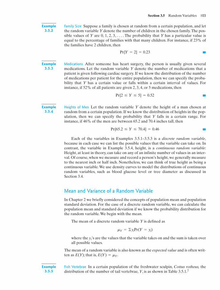
Family Size Suppose a family is chosen at random from a certain population, and letthe random variable Y denote the number of children in the chosen family.The pos-sible values of Y are 0, 1, 2, 3, . . . . The probability that Y has a particular value isequal to the percentage of families with that many children. For instance, if 23% ofthe families have 2 children, then

�

Medications After someone has heart surgery, the person is usually given severalmedications. Let the random variable Y denote the number of medications that apatient is given following cardiac surgery. If we know the distribution of the numberof medications per patient for the entire population, then we can specify the proba-bility that Y has a certain value or falls within a certain interval of values. Forinstance, if 52% of all patients are given 2, 3, 4, or 5 medications, then

�

Heights of Men Let the random variable Y denote the height of a man chosen atrandom from a certain population. If we know the distribution of heights in the pop-ulation, then we can specify the probability that Y falls in a certain range. Forinstance, if 46% of the men are between 65.2 and 70.4 inches tall, then

�

Each of the variables in Examples 3.5.1–3.5.3 is a discrete random variable,because in each case we can list the possible values that the variable can take on. Incontrast, the variable in Example 3.5.4, height, is a continuous random variable:Height, at least in theory, can take on any of an infinite number of values in an inter-val. Of course, when we measure and record a person’s height, we generally measureto the nearest inch or half inch. Nonetheless, we can think of true height as being acontinuous variable. We use density curves to model the distributions of continuousrandom variables, such as blood glucose level or tree diameter as discussed inSection 3.4.

Mean and Variance of a Random Variable

In Chapter 2 we briefly considered the concepts of population mean and populationstandard deviation. For the case of a discrete random variable, we can calculate thepopulation mean and standard deviation if we know the probability distribution forthe random variable. We begin with the mean.

The mean of a discrete random variable Y is defined as

where the yi’s are the values that the variable takes on and the sum is taken overall possible values.

The mean of a random variable is also known as the expected value and is often writ-ten as E(Y); that is, .

Fish Vertebrae In a certain population of the freshwater sculpin, Cottus rotheus, thedistribution of the number of tail vertebrae, Y, is as shown in Table 3.5.1.2

Example3.5.5

E(Y) = mY

mY = ©yiPr(Y = yi)

Pr{65.2 … Y … 70.4} = 0.46

Example3.5.4

Pr{2 … Y … 5} = 0.52

Example3.5.3

Pr{Y = 2} = 0.23

Example3.5.2


Table 3.5.1 Distribution of vertebrae

No. of vertebrae Percent of fish

20 3

21 51

22 40

23 6

Total 100

The mean of Y is

�

Dice Consider rolling a die that is perfectly balanced so that each of the six faces isequally likely to come up and let the random variable Y represent the number ofspots showing. The expected value, or mean, of Y is

�

To find the standard deviation of a random variable, we first find the variance,, of the random variable and then take the square root of the variance to get the

the standard deviation, .

The variance of a discrete random variable Y is defined as

where the yi’s are the values that the variable takes on and the sum is taken overall possible values.

We often write VAR(Y) to denote the variance of Y.

Fish Vertebrae Consider the distribution of vertebrae given in Table 3.5.1. InExample 3.5.5 we found that the mean of Y is . The variance of Y is

The standard deviation of Y is 0.6557. �sY = 10.4299 «

= 0.4299.

= 0.066603 + 0.122451 + 0.10404 + 0.136806

= 2.2201 * 0.03 + .2401 * 0.51 + .2601 * 0.40 + 2.2801 * 0.06

+ (0.51)2 * 0.40 + (1.51)2 * 0.06= (-1.49)2 * 0.03 + (- .49)2 * 0.51

+ (23 - 21.49)2 * Pr{Y = 23}+ (22 - 21.49)2 * Pr{Y = 22}+ (21 - 21.49)2 * Pr{Y = 21}

VAR(Y) = sY2 = (20 - 21.49)2 * Pr{Y = 20}

mY = 21.49Example

3.5.7

sY2 = ©(yi - mY)2Pr(Y = yi)

s

s2

E(Y) = mY = 1 *16

+ 2 *16

+ 3 *16

+ 4 *16

+ 5 *16

+ 6 *16

=216

= 3.5.

Example3.5.6

= 21.49.= 0.6 + 10.71 + 8.8 + 1.38= 20 * .03 + 21 * .51 + 22 * .40 + 23 * .06

mY = 20 * Pr{Y = 20} + 21 * Pr{Y = 21} + 22 * Pr{Y = 22} + 23 * Pr{Y = 23}

Section 3.5 Random Variables 105

Dice In Example 3.5.6 we found that the mean number obtained from rolling a fairdie is 3.5 (i.e., ). The variance of the number obtained from rolling a fairdie is

The standard deviation of Y is �

The preceding definitions are appropriate for discrete random variables. Thereare analogous definitions for continuous random variables, but they involve integralcalculus and won’t be presented here.

Adding and Subtracting Random Variables (Optional)

If we add two random variables, it makes sense that we add their means. Likewise, ifwe create a new random variable by subtracting two random variables, then wesubtract the individual means to get the mean of the new random variable. If wemultiply a random variable by a constant (for example, if we are converting feet toinches, so that we are multiplying by 12), then we multiply the mean of the randomvariable by the same constant. If we add a constant to a random variable, then weadd that constant to the mean.

The following rules summarize the situation:

Rules for Means of Random Variables

Rule (1) If X and Y are two random variables, then .

Rule (2) If Y is a random variable and a and b constants, then

Temperature The average summer temperature, , in a city is 81°F. To convert °F to°C, we use the formula Thus, the mean in degrees Celsius is

. �

Dealing with standard deviations of functions of random variables is a bit morecomplicated. We work with the variance first and then take the square root, at the

= 27.22(5/9) * (81) - (5/9) * 32 = 45 - 17.78

°C = (°F - 32) * (5/9) or °C = (5/9) * °F - (5/9) * 32.mYExample

3.5.9

ma+bY = a + bmY.

mX-Y = mX - mY

mX+Y = mX + mY

sY = 12.9167 L 1.708.

L 2.9167.

= 17.5 *16

+ (2.25) *16

+ (6.25) *16

= (6.25) *16

+ (2.25) *16

+ (0.25) *16

+ (0.25) *16

+ (1.5)2 *16

+ (2.5)2 *16

= (-2.5)2 *16

+ (-1.5)2 *16

+ (-0.5)2 *16

+ (0.5)2 *16

* Pr{Y = 5} + (6 - 3.5)2 * Pr{Y = 6}+ (5 - 3.5)2* Pr{Y = 3} + (4 - 3.5)2 * Pr{Y = 4}+ (3 - 3.5)2

sY2 = (1 - 3.5)2 * Pr{Y = 1} + (2 - 3.5)2 * Pr{Y = 2}

mY = 3.5Example

3.5.8


end, to get the standard deviation we want. If we multiply a random variable by aconstant (for example, if we are converting inches to centimeters by multiplying by2.54), then we multiply the variance by the square of the constant.This has the effectof multiplying the standard deviation by the constant. If we add a constant to a ran-dom variable, then we are not changing the relative spread of the distribution, so thevariance does not change.

Feet to Inches Let Y denote the height, in feet, of a person in a given population; sup-pose the standard deviation of Y is (feet). If we wish to convert from feetto inches, we can define a new variable X as . The variance of Y is 0.352

(the square of the standard deviation). The variance of X is 122 0.352, whichmeans that the standard deviation of X is �

If we add two random variables that are independent of one another, then weadd their variances.* Moreover, if we subtract two random variables that are inde-pendent of one another, then we add their variances. If we want to find the standarddeviation of the sum (or difference) of two independent random variables, we firstfind the variance of the sum (or difference) and then take the square root to get thestandard deviation of the sum (or difference).

Mass Consider finding the mass of a 10-ml graduated cylinder. If several measure-ments are made, using an analytical balance, then in theory we would expect themeasurements to all be the same. In reality, however, the readings will vary from onemeasurement to the next. Suppose that a given balance produces readings that havea standard deviation of 0.03g; let X denote the value of a reading made using thisbalance. Suppose that a second balance produces readings that have a standarddeviation of 0.04g; let Y denote denote the value of a reading made using thissecond balance.10

If we use each balance to measure the mass of a graduated cylinder, we might beinterested in the difference, , of the two measurements. The standard devia-tion of is positive. To find the standard deviation of , we first find thevariance of the difference. The variance of X is 0.032 and the variance of Y is 0.042.The variance of the difference is . The standard deviation of

is the square root of 0.0025, which is 0.05. �

The following rules summarize the situation for variances:

Rules for Variances of Random Variables

Rule (3) If Y is a random variable and a and b constants, then .

Rule (4) If X and Y are two independent random variables, then

sX-Y2 = sX2 + sY2sX+Y

2 = sX2 + sY2

sa+bY2 = b2sY

2

X - Y0.032 + 0.042 = 0.0025

X - YX - YX - Y

Example3.5.11

sX = 12 * 0.35 = 4.2 (inches).*

X = 12YsY = 0.35

Example3.5.10

*If we add two random variables that are not independent of one another, then the variance of the sum dependson the degree of dependence between the variables. To take an extreme case, suppose that one of the randomvariables is the negative of the other. Then the sum of the two random variables will always be zero, so that thevariance of the sum will be zero. This is quite different from what we would get by adding the two variancestogether. As another example, suppose Y is the number of questions correct on a 20-question exam and X is thenumber of questions wrong. Then Y X is always equal to 20, so that there is no variability at all. Hence, thevariance of Y X is zero, even though the variance of Y is positive, as is the variance of X.+

+

Section 3.6 The Binomial Distribution 107


3.5.1 In a certain population of the European starling,there are 5,000 nests with young. The distribution ofbrood size (number of young in a nest) is given in theaccompanying table.11

(a) Find (b) Find

3.5.5 Calculate the mean, , of the random variable Yfrom Exercise 3.5.4.

3.5.6 Calculate the standard deviation, , of the ran-dom variable Y from Exercise 3.5.4.

3.5.7 A group of college students were surveyed to learnhow many times they had visited a dentist in the previousyear.12 The probability distribution for Y, the number ofvisits, is given by the following table:

sY

mY

Pr{Y … 2}Pr{Y Ú 2}

Suppose one of the 5,000 broods is to be chosen at ran-dom, and let Y be the size of the chosen brood. Find(a) (b)(c)

3.5.2 In the starling population of Exercise 3.5.1, thereare 22,435 young in all the broods taken together. (Thereare 90 young from broods of size 1, there are 460 frombroods of size 2, etc.) Suppose one of the young is to bechosen at random, and let be the size of the chosenindividual’s brood.

(a) Find . (b) Find .

(c) Explain why choosing a young at random and thenobserving its brood is not equivalent to choosing abrood at random.Your explanation should show whythe answer to part (b) is greater than the answer topart (b) of Exercise 3.5.1.

3.5.3 Calculate the mean, , of the random variable Yfrom Exercise 3.5.1.

mY

Pr{Y¿ Ú 7}Pr{Y¿ = 3}

Y¿

Pr{4 … Y … 6}Pr{Y Ú 7}Pr{Y = 3}

Y (NO. BLACK) PROBABILITY

0 0.343

1 0.441

2 0.189

3 0.027

Total 1.000

Calculate the mean, , of the number of visits.

3.5.8 Calculate the standard deviation, , of the ran-dom variable Y from Exercise 3.5.7.

sY

mY

3.5.4 Consider a population of the fruitfly Drosophilamelanogaster in which 30% of the individuals are blackbecause of a mutation, while 70% of the individuals havethe normal gray body color. Suppose three flies are cho-sen at random from the population; let Y denote thenumber of black flies out of the three. Then the probabil-ity distribution for Y is given by the following table:

3.6 The Binomial DistributionTo add some depth to the notion of probability and random variables, we now con-sider a special type of random variable, the binomial. The distribution of a binomialrandom variable is a probability distribution associated with a special kind of

BROOD SIZE FREQUENCY (NO. OF BROODS)

1 90

2 230

3 610

4 1,400

5 1,760

6 750

7 130

8 26

9 3

10 1

Total 5,000

Y (NO. VISITS) PROBABILITY

0 0.15

1 0.50

2 0.35

Total 1.00


chance operation. The chance operation is defined in terms of a set of conditionscalled the independent-trials model.

The Independent-Trials Model

The independent-trials model relates to a sequence of chance “trials.” Each trial isassumed to have two possible outcomes, which are arbitrarily labeled “success” and“failure.” The probability of success on each individual trial is denoted by the letterp and is assumed to be constant from one trial to the next. In addition, the trials arerequired to be independent, which means that the chance of success or failure oneach trial does not depend on the outcome of any other trial. The total number oftrials is denoted by n. These conditions are summarized in the following definitionof the model.

Independent-Trials ModelA series of n independent trials is conducted. Each trial results in success or fail-ure. The probability of success is equal to the same quantity, p, for each trial,regardless of the outcomes of the other trials.

The following examples illustrate situations that can be described by the inde-pendent-trials model.

Albinism If two carriers of the gene for albinism marry, each of their children hasprobability 1/4 of being albino.The chance that the second child is albino is the same(1/4) whether or not the first child is albino; similarly, the outcome for the third childis independent of the first two, and so on. Using the labels “success” for albino and“failure” for nonalbino, the independent-trials model applies with and

. �

Mutant Cats A study of cats in Omaha, Nebraska, found that 37% of them have acertain mutant trait.13 Suppose that 37% of all cats have this mutant trait and that arandom sample of cats is chosen from the population. As each cat is chosen for thesample, the probability is 0.37 that it will be mutant. This probability is the same aseach cat is chosen, regardless of the results of the other cats, because the percentageof mutants in the large population remains equal to 0.37 even when a few individualcats have been removed. Using the labels “success” for mutant and “failure” fornonmutant, the independent-trials model applies with and

. �

An Example of the Binomial Distribution

The binomial distribution specifies the probabilities of various numbers of success-es and failures when the basic chance operation consists of n independent trials.Before giving the general formula for the binomial distribution, we consider asimple example.

sample sizen = thep = 0.37

Example3.6.2

n = the number of children in the familyp = 1/4

Example3.6.1


Albinism Suppose two carriers of the gene for albinism marry (see Example 3.6.1)and have two children. Then the probability that both of their children arealbino is

The reason for this probability can be seen by considering the relative frequencyinterpretation of probability. Of a great many such families with two children,would have the first child albino; furthermore, of these would have the secondchild albino; thus, of , or of all the couples would have both albino children. Asimilar kind of reasoning shows that the probability that both children are notalbino is

A new twist enters if we consider the probability that one child is albino and theother is not. There are two possible ways this can happen:

To see how to combine these possibilities, we again consider the relative frequencyinterpretation of probability. Of a great many such families with two children, thefraction of families with one albino and one nonalbino child would be the total ofthe two possibilities, or

Thus, the corresponding probability is

Another way to see this is to consider a probability tree.The first split in the treerepresents the birth of the first child; the second split represents the birth of the sec-ond child. The four possible outcomes and their associated probabilities are shownin Figure 3.6.1. These probabilities are collected in Table 3.6.1. �

The probability distribution in Table 3.6.1 is called the binomial distributionwith p and . Note that the probabilities add to 1.This makes sense becauseall possibilities have been accounted for: We expect of the families to have noalbino children, to have one albino child, and to have two albino children; thereare no other possible compositions for a two-child family.The number of albino chil-dren, out of the two children, is an example of a binomial random variable. Abinomial random variable is a random variable that satisfies the following four con-ditions, abbreviated as BInS:

116

616

916

n = 2= 14

Pr{one child is albino, the other is not} =616

a 316b + a 3

16b =

616

Pr{first child is not albino, second is} = a34b a1

4b =

316

Pr{first child is albino, second is not} = a14b a3

4b =

316

Pr{both children are not albino} = a34b a3

4b =

916

116

14

14

14

14

Pr{both children are albino} = a14b a1

4b =

116

Example3.6.3


1/4

1/4

3/4

1/4

3/4

3/4

Firstchildalbino

Firstchildnotalbino

Second childalbino

Second child notalbino

Second child albino

Second child not albino

116

316

316

916

Figure 3.6.1 Probabilitytree for albinism amongtwo children of carriers ofthe gene for albinism

Binary outcomes: There are two possible outcomes for each trial (success andfailure).

Independent trials: The outcomes of the trials are independent of each other.n is fixed: The number of trials, n, is fixed in advance.Same value of p: The probability of a success on a single trial is the same for all

trials.

The Binomial Distribution Formula

A general formula is available that can be used to calculate probabilities associatedwith a binomial random variable for any values of n and p. This formula can beproved using logic similar to that in Example 3.6.3. (The formula is discussed furtherin Appendix 3.1.) The formula is given in the accompanying box.

Table 3.6.1 Probability distribution for number of albino children

Number of

Albino Nonalbino Probability

0 2916

1 1616

2 01

16

1

The Binomial Distribution FormulaFor a binomial random variable Y, the probability that the n trials result in j suc-cesses (and failures) is given by the following formula:

Pr{j successes} = Pr{Y = j} = nCjpj(1 - p)n- j

n - j

The quantity nCj appearing in the formula is called a binomial coefficient. Eachbinomial coefficient is an integer depending on n and on j. Values of binomial coef-ficients are given in Table 2 at the end of this book and can be found by the formula

where x! (“x-factorial”) is defined for any positive integer x as

and . For more details, see Appendix 3.1.0! = 1

x! = x(x - 1)(x - 2) Á (2)(1)

nCj =n!

j!(n - j)!


Thus, for the binomial probabilities are as indicated in Table 3.6.2. Notice thepattern in Table 3.6.2: The powers of p ascend (0, 1, 2, 3, 4, 5) and the powers of( ) descend (5, 4, 3, 2, 1, 0). (In using the binomial distribution formula, remem-ber that for any nonzero x.)x0 = 11 - p

n = 5

The following example shows a specific application of the binomial distributionwith .

Mutant Cats Suppose we draw a random sample of five individuals from a large pop-ulation in which 37% of the individuals are mutants (as in Example 3.6.2).The prob-abilities of the various possible samples are then given by the binomial distributionformula with and ; the results are displayed in Table 3.6.3. Forinstance, the probability of a sample containing 2 mutants and 3 nonmutants is

10(0.37)2(0.63)3 L 0.34

p = 0.37n = 5

Example3.6.4

n = 5

j: 0 1 2 3 4 5

5Cj: 1 5 10 10 5 1

Table 3.6.2 Binomial probabilities for n = 5

Number of

Successes j Failures n - j Probability

0 5 1p0( )51 - p1 4 5p1( )41 - p2 3 10p2( )31 - p3 2 10p3( )21 - p4 1 5p4( )11 - p5 0 1p5( )01 - p

For example, for the binomial coefficients are as follows:n = 5

Table 3.6.3 Binomial distribution with and p = 0.37n = 5

Number of

Mutants Nonmutants Probability

0 5 0.10

1 4 0.29

2 3 0.34

3 2 0.20

4 1 0.06

5 0 0.01

1.00

Thus, .This means that about 34% of random samples of size 5 willcontain two mutants and three nonmutants.

Notice that the probabilities in Table 3.6.3 add to 1. The probabilities in a prob-ability distribution must always add to 1, because they account for 100% of thepossibilities. �

Pr{Y = 3} L 0.34


The binomial distribution of Table 3.6.3 is pictured graphically in Figure 3.6.2.The spikes in the graph emphasize that the probability distribution is discrete.

Remark In applying the independent-trials model and the binomial distribution, weassign the labels “success” and “failure” arbitrarily. For instance, in Example 3.6.4,we could say “success” = “mutant” and ; or, alternatively, we could say “suc-cess” = “nonmutant” and . Either assignment of labels is all right; it is onlynecessary to be consistent.

Notes on Table 2 The following features in Table 2 are worth noting:

(a) The first and last entries in each row are equal to 1. This will be true for anyrow; that is, and for any value of n.

(b) Each row of the table is symmetric; that is nCj and are equal.(c) The bottom rows of the table are left incomplete to save space, but you can

easily complete them using the symmetry of the nCj’s; if you need to know nCjyou can look up in Table 2. For instance, consider ; if you want toknow 18C15 you just look up 18C3; both 18C3 and 18C15 are equal to 816.

Computational note Computer and calculator technology makes it fairly easy tohandle the binomial distribution formula for small or moderate values of n. Forlarge values of n, the use of the binomial formula gets to be tedious and even acomputer will balk at being asked to calculate a binomial probability. However, thebinomial formula can be approximated by other methods. One of these will be dis-cussed in the optional Section 5.5.

Sometimes a binomial probability question involves combining two or morepossible outcomes. The following example illustrates this idea.

Sampling Fruitflies In a large Drosophila population, 30% of the flies are black (B)and 70% are gray (G). Suppose two flies are randomly chosen from the population(as in Example 3.2.3). The binomial distribution with and gives prob-abilities for the possible outcomes as shown in Table 3.6.4. (Using the binomial for-mula agrees with the results given by the probability tree shown in Figure 3.2.3.)

p = 0.3n = 2

Example3.6.5

n = 18nCn- j

nCn- j

nCn = 1nC0 = 1

p = 0.63p = 0.37

0.4

0.2

Pro

babi

lity

0.0

0 1 2

Number of mutants

3 4 5

Figure 3.6.2 Binomialdistribution with andp = 0.37

n = 5

Table 3.6.4

Sample composition Y Probability

Both G 0 0.49

One B, one G 1 0.42

Both B 2 0.09

1.00

Let E be the event that both flies are the same color. Then E can happen in twoways: Both flies are gray or both are black. To find the probability of E, considerwhat would happen if we repeated the sampling procedure many times: Forty-nine


percent of the samples would have both flies gray, and 9% would have both fliesblack. Consequently, the percentage of samples with both flies the same color wouldbe . Thus, we have shown that the probability of E is

as we claimed in Example 3.2.3. �

Whenever an event E can happen in two or more mutually exclusive ways, arationale such as that of Example 3.6.5 can be used to find Pr{E}.

Blood Type In the United States, 85% of the population has Rh positive blood. Sup-pose we take a random sample of 6 persons and count the number with Rh positiveblood. The binomial model can be applied here, since the BInS conditions are met:There is a binary outcome on each trial (Rh positive or Rh negative blood), the tri-als are independent (due to the random sampling), n is fixed at 6, and the sameprobability of Rh positive blood applies to each person ( ).

Let Y denote the number of persons, out of 6, with Rh positive blood.The prob-abilities of the possible values of Y are given by the binomial distribution formulawith and ; the results are displayed in Table 3.6.5. For instance, theprobability that is

If we want to find the probability that at least 4 persons (out of the 6 sampled)will have Rh positive blood, we need to find

. This means thatthe probability of getting at least 4 persons with Rh positive blood in a sample ofsize 6 is 0.9526. �

Pr{Y = 5} + Pr{Y = 6} = 0.1762 + 0.3993 + 0.3771 = 0.9526Pr{Y Ú 4} = Pr{Y = 4} +

6C4(0.85)4(0.15)2 L 15(0.522)(0.0225) L 0.1762

Y = 4p = 0.85n = 6

p = 0.85

Example3.6.6

Pr{E} = 0.58

49% + 9% = 58%

Table 3.6.5 Binomial distribution with and p = 0.85n = 6

Number of successes Probability

0 60.0001

1 0.0004

2 0.0055

3 0.0415

4 0.1762

5 0.3993

6 0.3771

1

In some problems, it is easier to find the probability that an event does nothappen rather than finding the probability of the event happening. To solve suchproblems we use the fact that the probability of an event happening is 1 minus theprobability that the event does not happen: .The following is an example.

Blood Type As in Example 3.6.6, let Y denote the number of persons, out of 6, withRh positive blood. Suppose we want to find the probability that Y is less than 6 (i.e.,the probability that there is at least 1 person in the sample who has Rh negativeblood). We could find this directly as .However, it is easier to find and subtract this from 1:

�Pr{Y 6 6} = 1 - Pr{Y = 6} = 1 - 0.3771 = 0.6229.

Pr{Y Z 6}Pr{Y = 0} + Pr{Y = 1} + Á + Pr{Y = 5}

Example3.6.7

Pr{E} = 1 - Pr{E does not happen}


Mean and Standard Deviation of a Binomial

If we toss a fair coin 10 times, then we expect to get 5 heads, on average. This is anexample of a general rule: For a binomial random variable, the mean (that is, theaverage number of successes) is equal to np. This is an intuitive fact: The probabilityof success on each trial is p, so if we conduct n trials, then np is the expected numberof successes. In Appendix 3.2 we show that this result is consistent with the rule givenin Section 3.5 for finding the mean of the sum of random variables. The standard de-viation for a binomial random variable is given by . This formula is notintuitively clear; a derivation of the result is given in Appendix 3.2. For the exampleof tossing a coin 10 times, the standard deviation of the number of heads is

Blood Type As discussed in Example 3.6.6, if Y denotes the number of persons withRh positive blood in a sample of size 6, then a binomial model can be used to findprobabilities associated with Y. The single most likely value of Y is 5 (which hasprobability 0.3993). The average value of Y is 6 � 0.85 = 5.1, which means that if wetake many samples, each of size 6, and count the number of Rh positive persons ineach sample, and then average those counts, we expect to get 5.1.The standard devi-ation of those counts is 0.87. �

Applicability of the Binomial Distribution

A number of statistical procedures are based on the binomial distribution. We willstudy some of these procedures in later chapters. Of course, the binomial distribu-tion is applicable only in experiments where the BInS conditions are satisfied in thereal biological situation. We briefly discuss some aspects of these conditions.

Application to Sampling The most important application of the independent-trials model and the binomial distribution is to describe random sampling from apopulation when the observed variable is dichotomous—that is, a categorical vari-able with two categories (for instance, black and gray in Example 3.6.5). This appli-cation is valid if the sample size is a negligible fraction of the population size, so thatthe population composition is not altered appreciably by the removal of the individ-uals in the sample (so that the S part of BInS is satisfied:The probability of a successremains the same from trial to trial). However, if the sample is not a negligibly smallpart of the population, then the population composition may be altered by the sam-pling process, so that the “trials” involved in composing the sample are not inde-pendent and the probability of a success changes as the sampling progresses. In thiscase, the probabilities given by the binomial formula are not correct. In most biolog-ical studies, the population is so large that this kind of difficulty does not arise.

Contagion In some applications the phenomenon of contagion can invalidate thecondition of independence between trials. The following is an example.

Chickenpox Consider the occurrence of chickenpox in children. Each child in a fam-ily can be categorized according to whether he had chickenpox during a certain year.One can say that each child constitutes a “trial” and that “success” is having chicken-pox during the year, but the trials are not independent because the chance of a partic-ular child catching chickenpox depends on whether his sibling caught chickenpox.As a specific example, consider a family with five children, and suppose that the

Example3.6.9

16 * 0.85 * .015 L

Example3.6.8

110 * 0.5 * 0.5 = 12.5 L 1.58.

2np(1 - p)


chance of an individual child catching chickenpox during the year is equal to 0.10.Thebinomial distribution gives the chance of all five children getting chickenpox as

However, this answer is not correct; because of contagion, the correct probabilitywould be much larger. There would be many families in which one child caughtchickenpox and then the other four children got chickenpox from the first child, sothat all five children would get chickenpox. �

Pr{5 children get chickenpox} = (0.10)5 = 0.00001


3.6.1 The seeds of the garden pea (Pisum sativum) areeither yellow or green. A certain cross between peaplants produces progeny in the ratio 3 yellow 1 green.14

If four randomly chosen progeny of such a cross areexamined, what is the probability that

(a) three are yellow and one is green?

(b) all four are yellow?

(c) all four are the same color?

3.6.2 In the United States, 42% of the population hastype A blood. Consider taking a sample of size 4. Let Ydenote the number of persons in the sample with type Ablood. Find

(a) .

(b) .

(c) .

(d) .

(e) .

3.6.3 A certain drug treatment cures 90% of cases ofhookworm in children.15 Suppose that 20 children suffer-ing from hookworm are to be treated, and that the chil-dren can be regarded as a random sample from thepopulation. Find the probability that

(a) all 20 will be cured.

(b) all but 1 will be cured.

(c) exactly 18 will be cured.

(d) exactly 90% will be cured.

3.6.4 The shell of the land snail Limocolaria martensianahas two possible color forms: streaked and pallid. In acertain population of these snails, 60% of the individualshave streaked shells.16 Suppose that a random sample of10 snails is to be chosen from this population. Find theprobability that the percentage of streaked-shelled snailsin the sample will be(a) 50%. (b) 60%. (c) 70%.

3.6.5 Consider taking a sample of size 10 from the snailpopulation in Exercise 3.6.4.(a) What is the mean number of streaked-shelled snails?(b) What is the standard deviation of the number of

streaked-shelled snails?

Pr{0 6 Y … 2}

Pr{0 … Y … 2}

Pr{Y = 2}

Pr{Y = 1}

Pr{Y = 0}

:

3.6.6 The sex ratio of newborn human infants is about105 males 100 females.17 If four infants are chosen atrandom, what is the probability that

(a) two are male and two are female?

(b) all four are male?

(c) all four are the same sex?

3.6.7 Construct a binomial setting (different from anyexamples presented in this book) and a problem forwhich the following is the answer: 7C3(0.8)3(0.2)5.

3.6.8 Neuroblastoma is a rare, serious, but treatable dis-ease. A urine test, the VMA test, has been developedthat gives a positive diagnosis in about 70% of cases ofneuroblastoma.18 It has been proposed that this test beused for large-scale screening of children. Assume that300,000 children are to be tested, of whom 8 have the dis-ease. We are interested in whether or not the test detectsthe disease in the 8 children who have the disease. Findthe probability that

(a) all eight cases will be detected.

(b) only one case will be missed.

(c) two or more cases will be missed. [Hint: Use parts (a)and (b) to answer part (c).]

3.6.9 If two carriers of the gene for albinism marry, eachof their children has probability of being albino (seeExample 3.6.1). If such a couple has six children, what isthe probability that

(a) none will be albino?

(b) at least one will be albino? [Hint: Use part (a) to answerpart (b); note that “at least one” means “one or more.”]

3.6.10 Childhood lead poisoning is a public health con-cern in the United States. In a certain population, 1 childin 8 has a high blood lead level (defined as 30 μg/dl ormore).19 In a randomly chosen group of 16 children fromthe population, what is the probability that

(a) none has high blood lead?

(b) 1 has high blood lead?

(c) 2 have high blood lead?

(d) 3 or more have high blood lead? [Hint: Use parts(a)–(c) to answer part (d).]

14

:


3.7 Fitting a Binomial Distribution to Data (Optional)Occasionally it is possible to obtain data that permit a direct check of the applicabil-ity of the binomial distribution. One such case is described in the next example.

Sexes of Children In a classic study of the human sex ratio, families were categorizedaccording to the sexes of the children. The data were collected in Germany in thenineteenth century, when large families were common. Table 3.7.1 shows the resultsfor 6,115 families with 12 children.20

It is interesting to consider whether the observed variation among families canbe explained by the independent-trials model. We will explore this question by fit-ting a binomial distribution to the data.

Example3.7.1

Table 3.7.1 Sex ratios in 6,115 families withtwelve children

Number of Observed frequency (number of families)Boys Girls

0 12 3

1 11 24

2 10 104

3 9 286

4 8 670

5 7 1,033

6 6 1,343

7 5 1,112

8 4 829

9 3 478

10 2 181

11 1 45

12 0 7

6,115

The first step in fitting the binomial distribution is to determine a value for. One possibility would be to assume that . However, since it is

known that the human sex ratio at birth is not exactly (in fact, it favors boysslightly), we will not make this assumption. Rather, we will “fit” p to the data; that is,we will determine a value for p that fits the data best. We observe that the totalnumber of children in all the families is

Among these children, the number of boys is

Therefore, the value of p that fits the data best is

p =38,10073,380

= 0.519215

(3)(0) + (24)(1) + Á + (12)(7) = 38,100 boys

(12)(6,115) = 73,380 children

1 : 1p = 0.50p = Pr{boy}

Section 3.7 Fitting a Binomial Distribution to Data (Optional) 117

The next step is to compute probabilities from the binomial distributionformula with and . For instance, the probability of 3 boys and 9girls is computed as

For comparison with the observed data, we convert each probability to atheoretical or “expected” frequency by multiplying by 6,115 (the total number offamilies). For instance, the expected number of families with 3 boys and 9 girls is

The expected and observed frequencies are displayed together in Table 3.7.2. Table3.7.2 shows reasonable agreement between the observed frequencies and the pre-dictions of the binomial distribution. But a closer look reveals that thediscrepancies, although not large, follow a definite pattern. The data contain moreunisexual, or preponderantly unisexual, sibships than expected. In fact, the observedfrequencies are higher than the expected frequencies for nine types of families inwhich one sex or the other predominates, while the observed frequencies are lowerthan the expected frequencies for four types of more “balanced” families. Thispattern is clearly revealed by the last column of Table 3.7.2, which shows the sign ofthe difference between the observed frequency and the expected frequency.Thus, the observed distribution of sex ratios has heavier “tails” and a lighter“middle” than the best-fitting binomial distribution.

The systematic pattern of deviations from the binomial distribution suggeststhat the observed variation among families cannot be entirely explained by the independent-trials model.* What factors might account for the discrepancy?

(6,115)(0.042269) L 258.5

L 0.04226912C3(p)3(1 - p)9 = 220(0.519215)3(0.480785)9

p = 0.519215n = 12

Table 3.7.2 Sex-ratio data and binomial expected frequencies

Number ofObservedfrequency

Expectedfrequency

Sign of ( )Obs. - Exp.Boys Girls

0 12 3 0.9 +1 11 24 12.1 +2 10 104 71.8 +3 9 286 258.5 +4 8 670 628.1 +5 7 1,033 1,085.2 -6 6 1,343 1,367.3 -7 5 1,112 1,265.6 -8 4 829 854.3 -9 3 478 410.0 +

10 2 181 132.8 +11 1 45 26.1 +12 0 7 2.3 +

6,115 6,115.0

*A chi-square goodness-of-fit test of the binomial model shows that there is strong evidence that the differencesbetween the observed and expected frequencies did not happen due to chance error in the sampling process.Wewill explore the topic of goodness-of-fit tests in Chapter 9.


This intriguing question has stimulated several researchers to undertake more de-tailed analysis of these data. We briefly discuss some of the issues.

One explanation for the excess of predominantly unisexual families is that theprobability of producing a boy may vary among families. If p varies from one familyto another, then sex will appear to “run” in families in the sense that the number ofpredominantly unisexual families will be inflated. In order to clearly visualize thiseffect, consider the fictitious data set shown in Table 3.7.3.

In the fictitious data set, there are males among 73,380children, just as there are in the real data set. Consequently, the best-fitting p is thesame ( ) and the expected binomial frequencies are the same as inTable 3.7.2. The fictitious data set contains only unisexual sibships and so is anextreme example of sex “running” in families. The real data set exhibits the samephenomenon more weakly. One explanation of the fictitious data set would bethat some families can have only boys ( ) and other families can have only girls( ). In a parallel way, one explanation of the real data set would be that p varies slightly among families. Variation in p is biologically plausible, even thoughthe mechanism causing the variation has not yet been discovered.

An alternative explanation for the inflated number of sexually homogeneousfamilies would be that the sexes of the children in a family are literally dependenton one another, in the sense that the determination of an individual child’s sex issomehow influenced by the sexes of the previous children. This explanation isimplausible on biological grounds because it is difficult to imagine how the biologi-cal system could “remember” the sexes of previous offspring. �

Example 3.7.1 shows that poorness of fit to the independent-trials model canbe biologically interesting. We should emphasize, however, that most statisticalapplications of the binomial distribution proceed from the assumption that theindependent-trials model is applicable. In a typical application, the data areregarded as resulting from a single set of n trials. Data such as the family sex-ratiodata, which refer to many sets of trials, are not often encountered.n = 12

p = 0p = 1

p = 0.519215

(3,175)(12) = 38,100

Table 3.7.3 Fictitious sex-ratio data and binomial expected frequencies

Number of Observedfrequency

Expectedfrequency

Sign of ( )Obs. - Exp.Boys Girls

0 12 2,940 0.9 +1 11 0 12.1 -2 10 0 71.8 -3 9 0 258.5 -4 8 0 628.1 -5 7 0 1,085.2 -6 6 0 1,367.3 -7 5 0 1,265.6 -8 4 0 854.3 -9 3 0 410.0 -

10 2 0 132.8 -11 1 0 26.1 -12 0 3,175 2.3 +

6,115 6,115.0

Section 3.7 Fitting a Binomial Distribution to Data (Optional) 119


3.7.1 The accompanying data on families with 6 childrenare taken from the same study as the families with 12children in Example 3.7.1. Fit a binomial distribution tothe data. (Round the expected frequencies to one deci-mal place.) Compare with the results in Example 3.7.1.What features do the two data sets share?

NUMBER OF

BOYS GIRLS NUMBER OF FAMILIES

0 6 1,096

1 5 6,233

2 4 15,700

3 3 22,221

4 2 17,332

5 1 7,908

6 0 1,579

72,069

NUMBER OF EMBRYOS NUMBER OF FEMALE MICEDEAD LIVING

0 9 136

1 8 103

2 7 50

3 6 13

4 5 6

5 4 1

6 3 1

7 2 0

8 1 0

9 0 0

310

3.7.2 An important method for studying mutation-causing substances involves killing female mice 17 daysafter mating and examining their uteri for living and deadembryos. The classical method of analysis of such dataassumes that the survival or death of each embryo consti-tutes an independent binomial trial. The accompanyingtable, which is extracted from a larger study, gives datafor 310 females, all of whose uteri contained 9 embryos;all of the animals were treated alike (as controls).21

NUMBER OF SEEDS NUMBER OF STUDENTSGERMINATED NOT GERMINATED

0 5 17

1 4 53

2 3 94

3 2 79

4 1 33

5 0 4

280

(a) Fit a binomial distribution to the observed data.(Round the expected frequencies to one decimalplace.)

(b) Interpret the relationship between the observed andexpected frequencies. Do the data cast suspicion onthe classical assumption?

3.7.3 Students in a large botany class conducted anexperiment on the germination of seeds of the Saguarocactus. As part of the experiment, each student plantedfive seeds in a small cup, kept the cup near a window, andchecked every day for germination (sprouting). The classresults on the seventh day after planting were as dis-played in the table.22

(a) Fit a binomial distribution to the data. (Round theexpected frequencies to one decimal place.)

(b) Two students, Fran and Bob, were talking beforeclass. All of Fran’s seeds had germinated by the sev-enth day, whereas none of Bob’s had. Bob wonderedwhether he had done something wrong.With the per-spective gained from seeing all 280 students’ results,what would you say to Bob? (Hint: Can the variationamong the students be explained by the hypothesisthat some of the seeds were good and some werepoor, with each student receiving a randomly chosenfive seeds?)

(c) Invent a fictitious set of data for 280 students, withthe same overall percentage germination as theobserved data given in the table, but with all thestudents getting either Fran’s results (perfect) orBob’s results (nothing). How would your answer toBob differ if the actual data had looked like this ficti-tious data set?

Supplementary Exercises 3.S.1–3.S.10

3.S.1 In the United States, 10% of adolescent girls haveiron deficiency.23 Suppose two adolescent girls are chosenat random. Find the probability that

(a) both girls have iron deficiency.(b) one girl has iron deficiency and the other does not.


NUMBER OF CENTIPEDES

PERCENT FREQUENCY(% OF SQUARES)

0 451 36

2 14

3 4

4 1

100

80 100 120

0.20 0.41 0.25 0.09

140 160

Blood pressure (mmHg)

180 200 220 240

0.040.01

3.S.7 Refer to Exercise 3.S.6. Suppose now that the drugis to be tested on n patients, and let E represent the eventthat kidney damage occurs in one or more of the patients.The probability Pr{E} is useful in establishing criteria fordrug safety.(a) Find Pr{E} for .

(b) How large must n be in order for Pr{E} to exceed0.95?

3.S.8 To study people’s ability to deceive lie detectors,researchers sometimes use the “guilty knowledge” tech-nique.26 Certain subjects memorize six common words;other subjects memorize no words. Each subject is thentested on a polygraph machine (lie detector), as follows.The experimenter reads, in random order, 24 words: thesix “critical” words (the memorized list) and, for eachcritical word, three “control” words with similar orrelated meanings. If the subject has memorized thesix words, he or she tries to conceal that fact. The subjectis scored a “failure” on a critical word if his or herelectrodermal response is higher on the critical wordthan on any of the three control words. Thus, on each ofthe six critical words, even an innocent subjectwould have a 25% chance of failing. Suppose a subject islabeled “guilty” if the subject fails on four or more of thesix critical words. If an innocent subject is tested, what isthe probability that he or she will be labeled “guilty”?

3.S.9 The density curve shown here represents thedistribution of systolic blood pressures in a populationof middle-aged men.27 Areas under the curveare shown in the figure. Suppose a man is selected atrandom from the population, and let Y be his blood pres-sure. Find

(a)

(b)

(c) Pr{Y > 140}.

Pr{Y < 120}.

Pr{120 < Y < 160}.

n = 100

3.S.2 In preparation for an ecological study of centipedes,the floor of a beech woods is divided into a large numberof 1-foot squares.24 At a certain moment, the distributionof centipedes in the squares is as shown in the table.

Suppose that a square is chosen at random, and let Y bethe number of centipedes in the chosen square. Find(a) (b)

3.S.3 Refer to the distribution of centipedes given inExercise 3.S.2. Suppose five squares are chosen atrandom. Find the probability that three of the squarescontain centipedes and two do not.

3.S.4 Refer to the distribution of centipedes given inExercise 3.S.2. Suppose five squares are chosen atrandom. Find the expected value (i.e., the mean) of thenumber of squares that contain at least one centipede.

3.S.5 Wavy hair in mice is a recessive genetic trait. Ifmice with wavy hair are mated with straight-haired(heterozygous) mice, each offspring has probability ofhaving wavy hair.25 Consider a large number of suchmatings, each producing a litter of five offspring. Whatpercentage of the litters will consist of(a) two wavy-haired and three straight-haired offspring?(b) three or more straight-haired offspring?(c) all the same type (either all wavy- or all straight-

haired) offspring?

3.S.6 A certain drug causes kidney damage in 1% ofpatients. Suppose the drug is to be tested on 50 patients.Find the probability that(a) none of the patients will experience kidney damage.(b) one or more of the patients will experience kidney

damage. [Hint: Use part (a) to answer part (b).]

12

Pr{Y Ú 2}Pr{Y = 1}

3.S.10 Refer to the blood pressure distribution of Exer-cise 3.S.9. Suppose four men are selected at random fromthe population. Find the probability that(a) all four have blood pressures higher than 140 mm Hg.(b) three have blood pressures higher than 140, and one

has blood pressure 140 or less.

Chapter 3 - PROBABILITY AND THE BINOMIAL DISTRIBUTION

Documents

Transcript of Chapter 3 - PROBABILITY AND THE BINOMIAL DISTRIBUTION