Some applications of the fractional Poisson probability distribution

$: Some applications of the fractional Poisson probability distribution$
arX

iv:0

812.

1193

v2 [

mat

h-ph

] 1

7 N

ov 2

011 Some Applications of the Fractional

Poisson Probability Distribution

Nick Laskin∗

TopQuark Inc.Toronto, ON, M6P 2P2

Canada

Abstract

Physical and mathematical applications of fractional Poisson prob-ability distribution have been presented. As a physical application, anew family of quantum coherent states has been introduced and stud-ied. As mathematical applications, we have discovered and developedthe fractional generalization of Bell polynomials, Bell numbers, andStirling numbers. Appearance of fractional Bell polynomials is nat-ural if one evaluates the diagonal matrix element of the evolutionoperator in the basis of newly introduced quantum coherent states.Fractional Stirling numbers of the second kind have been applied toevaluate skewness and kurtosis of the fractional Poisson probabilitydistribution function. A new representation of Bernoulli numbers interms of fractional Stirling numbers of the second kind has been ob-tained. A representation of Schlafli polynomials in terms of fractionalStirling numbers of the second kind has been found. A new repre-sentations of Mittag-Leffler function involving fractional Bell polyno-mials and fractional Stirling numbers of the second kind have beendiscovered. Fractional Stirling numbers of the first kind have been in-troduced and studied. Two new polynomial sequences associated withfractional Poisson probability distribution have been launched and ex-plored. The relationship between new polynomials and the orthogonalCharlier polynomials has also been investigated.

∗E-mail address : [email protected]

1

http://arxiv.org/abs/0812.1193v2

In the limit case when the fractional Poisson probability distri-bution becomes the Poisson probability distribution, all of the abovelisted developments and implementations turn into the well-known re-sults of quantum optics, the theory of combinatorial numbers and thetheory of orthogonal polynomials of discrete variable.

PACS numbers: 05.10.Gg; 05.45.Df; 42.50.-p.Keywords: fractional Poisson process, generalized quantum coher-

ent states, generating functions, fractional Stirling and Bell numbers,Mittag-Leffler function, Charlier orthogonal polynomials.

Contents

1 Introduction 3

2 Fundamentals of the fractional Poisson probability distribu-

tion 6

3 New family of coherent states 9

3.1 Quantum mechanical vector and operator representations basedon coherent states |ς > . . . . . . . . . . . . . . . . . . . . . . 15

4 Generalized Bell and Stirling Numbers 17

4.1 Fractional Bell polynomials and fractional Bell numbers . . . . 174.1.1 Quantum physics application of the fractional Bell poly-

nomials . . . . . . . . . . . . . . . . . . . . . . . . . . 204.1.2 Fractional compound Poisson processes . . . . . . . . . 22

4.2 Fractional Stirling numbers of the second kind . . . . . . . . . 284.2.1 A new representation for the Mittag-Leffler function . . 344.2.2 The Bernoulli numbers and fractional Stirling numbers

of the second kind . . . . . . . . . . . . . . . . . . . . 374.2.3 The Schlafli polynomials and fractional Stirling num-

bers of the second kind . . . . . . . . . . . . . . . . . . 384.3 Fractional Stirling numbers of the first kind . . . . . . . . . . 41

5 Statistics of the fractional Poisson probability distribution 43

5.1 Moments of the fractional Poisson probability distribution . . 435.2 Variance, skewness and kurtosis of the fractional Poisson prob-

ability distribution . . . . . . . . . . . . . . . . . . . . . . . . 45

2

6 New polynomials 46

6.1 Generating functions . . . . . . . . . . . . . . . . . . . . . . . 466.1.1 Multiplicative renormalization framework . . . . . . . . 466.1.2 Alternative approach . . . . . . . . . . . . . . . . . . . 54

7 Conclusions 56

8 Appendix 57

1 Introduction

In the past decade it has been realized that modeling complex quantumand classical physics phenomena requires the implementation of long-rangespace and long-memory stochastic processes. The mathematical model tocapture impact of long-range phenomena at a quantum level is the Levy path

integral approach invented and studied in Refs.[1]-[6]. The Levy path integralapproach generalizes the path integral formulation of quantum mechanicsdeveloped in 1948 by Feynman [7], [8]. The generalization results in fractional

quantum mechanics [1]-[3]. One of the fundamental equations of fractionalquantum mechanics is the fractional Schrodinger equation discovered in [1]-[4], [6]. The fractional Schrodinger equation is a new non-Gaussian physicalparadigm, based on deep relationships between the structure of fundamentalphysics equations and fractal dimensions of “underlying” quantum paths.

To study a long-memory impact on the counting process, the fractional

Poisson process has been invented and developed for the first time by Laskinin Ref.[9]. The fractional Poisson probability distribution captures the long-memory effect which results in the non-exponential waiting time probabil-ity distribution function [9], empirically observed in complex quantum andclassical systems. The quantum system example is the fluorescence inter-mittency of single CdSe quantum dots, that is, the fluorescence emissionof single nanocrystals exhibits intermittent behavior, namely, a sequence of”light on” and ”light off” states departing from Poisson statistics. In fact,the waiting time distribution in both states is non-exponential [10]. As ex-amples of classical systems let’s mention the distribution of waiting timesbetween two consecutive transactions in financial markets [11] and another,which comes from network communication systems, where the duration ofnetwork sessions or connections exhibits non-exponential behavior [12].

3

The non-exponential waiting time distribution function has been obtainedfor the first time in Ref.[13], based on the fractional generalization of thePoisson exponential waiting time distribution.

The fractional Poisson process is a natural generalization of the wellknown Poisson process. A simple analytical formula for the fractional Pois-son probability distribution function has been obtained for the first timein Ref.[9] based on the fractional generalization of the Kolmogorov-Fellerequation introduced in Ref.[13]. It was shown by Laskin in [9] that the non-exponential waiting time distribution function of fractional Poisson processobtained in [9] is identical to the one found in [13].

In comparison to standard Poisson distribution, the probability distribu-tion function of the fractional Poisson process [9] has an additional parameterµ, 0 < µ ≤ 1. In the limit case µ = 1 the fractional Poisson process becomesthe standard Poisson process and all our findings are transformed into thewell-known results related to the standard Poisson probability distribution.

Now we present quantum physics and mathematical applications of thefractional Poisson probability distribution [14]. This paper is an extendedversion of articles [14], [15].

The quantum physics application is an introduction of a new family ofquantum coherent states. The motivation to introduce and explore thesecoherent states is the observation that the squared modulus | < n|ς > |2of projection of the newly invented coherent state |ς > onto the eigenstateof the photon number operator |n > gives us the fractional Poisson proba-bility Pµ(n) that n photons will be found in coherent state |ς > . FollowingKlauder’s framework to qualify quantum states as generalized coherent states[16], we prove that our quantum coherent states |ς >, (i) are parametrizedcontinuously and normalized; (ii) admit a resolution of unity with positiveweight function; (iii) provide temporal stability, that is, the time evolutionof coherent states remains within the family of coherent states. We havedefined the inner product of two vectors in terms of their coherent state |ς >representation and introduced functional Hilbert space.

Mathematical applications are related to number theory and theory ofpolynomials of discrete variable. Bell polynomials, Bell numbers [17] andStirling numbers [18] - [20] have been generalized based on the fractionalPoisson probability distribution. In other words, based on fractional Pois-son probability distribution, we introduce new fractional Bell polynomials,new fractional Bell numbers and new fractional Stirling numbers in the samefashion as the well-known Bell polynomials, Bell numbers and Stirling num-

4

bers can be introduced based on the famous Poisson probability distribu-tion. Appearance of fractional Bell polynomials is natural if one evaluatesthe diagonal matrix element of the quantum evolution operator in the basisof newly introduced quantum coherent states. The appearance of fractionalBell numbers manifests itself in the fractional generalization of the celebratedDobinski formula [21], [22] for the generating function of the Bell numbers.

Fractional Stirling numbers of the second kind have been applied to eval-uate skewness and kurtosis of the fractional Poisson probability distribution.

Fractional Stirling numbers of the first kind have also been introducedand studied.

A representation of Schlafli polynomials in terms of fractional Stirlingnumbers of the second kind has been found. The integral relationship be-tween the Schlafli polynomials and fractional Bell polynomials has been ob-tained. A new representation of the Mittag-Leffler function involving frac-tional Bell polynomials and fractional Stirling numbers of the second kindhas been discovered.

New polynomials of discrete variable associated with fractional Poissonprobability distribution have been launched and explored in the multiplica-tive renormalization [23] framework.

In the limit case when µ = 1 and the fractional Poisson probability dis-tribution becomes the standard Poisson probability distribution, all abovelisted new developments and findings turn into the well-known results of thequantum coherent states theory [24]-[26], the theory of combinatorial num-bers [19], [20] and the theory of orthogonal polynomilas of discrete variable[27].

The paper is organized as follows.Basic definitions of the fractional Poisson random process are briefly re-

viewed in Sec.2, where Table 1 has been presented to compare the formulasrelated to the fractional Poisson probability distribution [9] to those of thewell-known ones, related to the standard Poisson probability distribution. InSec.3 we introduce and study new quantum coherent states and their ap-plications. Fractional generalizations of Bell polynomials, Bell numbers andStirling numbers have been introduced and developed in Sec.4. New equa-tions for the generating functions of fractional Bell polynomials, fractionalBell numbers and fractional Stirling numbers have been obtained and elab-orated. The relationship between Bernoulli numbers and fractional Stirlingnumbers of the second kind has been found. A new representation of theSchlafli polynomials in terms of fractional Stirling numbers of the second

5

kind has been found. The integral relationship between the Schlafli polyno-mials and fractional Bell polynomials has been found. A new representationsof the Mittag-Leffler function involving fractional Bell polynomials and frac-tional Stirling numbers of the second kind have been discovered and explored.Fractional Stirling numbers of the first kind have also been introduced andstudied in Sec.4.

Moments and central moments of the fractional Poisson probability distri-bution have been studied in Sec.5. The central moment of m-order has beenobtained in terms of fractional Stirling numbers of the second kind. Vari-ance, skewness and kurtosis of the fractional Poisson probability distributionfunction have been presented in terms of the central moments of m-order.

A new class of polynomials of discrete variable associated with fractionalPoisson probability distribution have been launched and explored in Sec.6. Ithas been observed that in the limit case when µ = 1, these new polynomialsbecome the well-known Charlier orthogonal polynomials [27].

Table 2 summarizes key fundamental equations of the coherent states the-ory for new coherent states |ς > vs those for standard coherent states |z >.Table 3 displays the moment generating functions of four fractional com-pound Poisson processes. Table 4 presents a few fractional Stirling numbersof the second kind. Table 5 presents polynomials, numbers, moments andgenerating functions attributed to the fractional Poisson probability distri-bution vs the standard Poisson probability distribution. Table 6 presents afew fractional Stirling numbers of the first kind. Table 7 compares fundamen-tals for newly introduced polynomials Ln(x;λµ) vs the Charlier orthogonalpolynomials Cn(x;λ).

2 Fundamentals of the fractional Poisson prob-

ability distribution

The fractional Poisson process has originally been introduced and developedby Laskin [9] as the counting process with probability Pµ(n, t) of arrivingn items (n = 0, 1, 2, ...) by time t. Probability Pµ(n, t) is governed by thesystem of fractional differential-difference equations

0Dµt Pµ(n, t) = ν (Pµ(n− 1, t)− Pµ(n, t)) , n ≥ 1, (1)

and

6

0Dµt Pµ(0, t) = −νPµ(0, t) +

t−µ

Γ(1− µ), 0 < µ ≤ 1, (2)

with normalization condition

∞∑

n=0

Pµ(n, t) = 1. (3)

Here, 0Dµt is the operator of time derivative of fractional order µ defined

as the Riemann-Liouville integral1,

0Dµt f(t) =

1

Γ(1− µ)

d

dt

t∫

0

dτ f(τ )

(t− τ )µ, 0 < µ ≤ 1,

where µ is the fractality parameter, gamma function Γ(µ) has the fa-

miliar representation Γ(µ) =∞∫

0

dte−ttµ−1, Reµ > 0, and parameter ν has

physical dimension [ν] = sec−µ. The system introduced by Eqs.(1) and (2)has the initial condition Pµ(n, t = 0) = δn,0. One can consider the fractionaldifferential-difference system of equations (1) and (2) as a generalization ofthe differential-difference equations which define the well-known Poisson pro-cess (see, for instance, Eqs.(6) and (7) in Ref.[9]).

To solve the system of equations (1) and (2) it is convenient to use themethod of the generating function. We introduce the generating functionGµ(s, t)

Gµ(s, t) =∞∑

n=0

snPµ(n, t). (4)

Hence, to obtain Pµ(n, t) we have to calculate

Pµ(n, t) =1

n!

∂nGµ(s, t)

∂sn|s=0. (5)

Then, by multiplying Eqs.(1) and (2) by sn, summing over n, we ob-tain the following fractional differential equation for the generating functionGµ(s, t)

1The basic formulas on fractional calculus can be found in Refs. [28] - [30].

7

0Dµt Gµ(s, t) = ν

( ∞∑

n=0

snPµ(n− 1, t)−∞∑

n=0

snPµ(n, t)

)

= (6)

ν(s− 1)Gµ(s, t) +t−µ

Γ(1− µ).

The solution of this fractional differential equation has been found in [9]

Gµ(s, t) = Eµ(νtµ(s− 1)), (7)

where Eµ(z) is the Mittag-Leffler function2 given by its power series [31],[32]

Eµ(z) =

∞∑

m=0

zm

Γ(µm+ 1). (8)

It follows from Eqs.(5), (7) and (8) that

Pµ(n, t) =(νtµ)n

n!

∞∑

k=0

(k + n)!

k!

(−νtµ)kΓ(µ(k + n) + 1)

, 0 < µ ≤ 1. (9)

This is the fractional Poisson probability distribution obtained for thefirst time by Laskin in [9]. It gives us the probability that in the timeinterval [0, t] we observe n counting events. When µ = 1, Pµ(n, t) is trans-formed to the standard Poisson probability distribution function (see Eq.(14)in Ref.[9]). Thus, Eq.(9) can be considered as a fractional generalization ofthe well-known Poisson probability distribution function. The presence of anadditional parameter µ brings new features in comparison with the standardPoisson probability distribution.

On a final note, the probability distribution of the fractional Poissonprocess Pµ(n, t) can be represented in terms of the Mittag-Leffler functionEµ(z) in the following compact way [9],

Pµ(n, t) =(−z)nn!

dn

dznEµ(z)|z=−νtµ , (10)

Pµ(n = 0, t) = Eµ(−νtµ). (11)

2At µ = 1 the function Eµ(z) turns into exp(z).

8

At µ = 1 Eqs.(10) and (11) are transformed into the well known equationsfor the famous Poisson probability distribution P (n, t) with the substitutionν → ν, where ν is the rate of arrivals of the Poisson process with physicaldimension ν = sec−1,

Pµ(n, t)|µ=1 = P (n, t) =(νt)n

n!e−νt, (12)

P (n = 0, t) = e−νt. (13)

Table 1 compares equations attributed to the fractional Poisson processwith those belonging to the well-known standard Poisson process. Table 1presents two sets of equations for the probability distribution function P (n, t)of n events having arrived by time t, the probability P (0, t) of having nothingarrived by time t, mean n, variance σ2, generating function G(s, t) for theprobability distribution function, moment generating function H(s, t), andthe waiting-time probability distribution function ψ(τ ).

fractional Poisson (0 < µ ≤ 1) Poisson (µ = 1)

P (n, t) (νtµ)n

n!

∞∑

k=0

(k+n)!k!

(−νtµ)k

Γ(µ(k+n)+1)(νt)n

n!exp(−νt)

P (n, t) (−z)n

n!dn

dznEµ(z)|z=−νtµ

(−z)n

n!dn

dznexp(z)|z=−νtµ

P (0, t) Eµ(−νtµ) exp(−νt)n νtµ

Γ(µ+1)νt

σ2 νtµ

Γ(µ+1)+(

νtµ

Γ(µ+1)

)2 {µB(µ, 12)

22µ−1 − 1}

νt

G(s, t) Eµ(νtµ(s− 1)) exp{νt(s− 1)}

H(s, t) Eµ(νtµ(e−s − 1)) exp{νt(e−s − 1)}

ψ(τ ) ντµ−1Eµ,µ(−ντµ) νe−ντ

Table 1. Fractional Poisson process vs the Poisson process3.

3 New family of coherent states

The quantum mechanical states first introduced by Schrodinger [33] to studythe quantum harmonic oscillator are now well-known as the coherent states.Coherent states provide an important theoretical paradigm to study electro-magnetic field coherence and quantum optics phenomena [24], [25].

3All definitions and equations related to the fractional Poisson process are taken from[9].

9

The standard coherent states are defined for all complex numbers z ∈ C,by

|z >= e(za+−z∗a)|0 >= e−

12|z|2

∞∑

n=0

zn√n!|n >, (14)

where a+ and a are photon field creation and annihilation operators thatsatisfy the Bose-Einstein commutation relation [a, a+] = aa+− a+a = 1, andthe orthonormal vector |n >= 1√

n!(a+)n|0 > is an eigenvector of the photon

number operator N = a+a, N |n >= n|n >, < n|n′ >= δn,n′. The action ofthe operators a+ and a act on the state |n > reads

a+|n >=√n + 1|n+ 1 > and a|n >=

√n|n− 1 > .

The projection of coherent state |z > onto state |n > is

< n|z >= zn√n!e−

12|z|2. (15)

Then the squared modulus of < n|z > gives us probability P (n) thatn photons will be found in the coherent state |z >. Thus, we come to thewell-know result for probability P (n)

P (n) = | < n|z > |2 = |z|2nn!

e−|z|2, (16)

which is recognized as a Poisson probability distribution with a meanvalue |z|2. The value |z|2 is in fact the mean number of photons when thestate is a coherent state |z >

|z|2 =∞∑

n=0

nP (n) =< z|a+a|z > . (17)

We introduce a new family of coherent states |ς >

|ς >=∞∑

n=0

(√µςµ)n√n!

(E(n)µ (−µ|ς|2µ))1/2|n >, (18)

and adjoint states < ς |

< ς| =∞∑

n=0

< n|(√µς∗µ)n√n!

(E(n)µ (−µ|ς|2µ))1/2, (19)

10

where

E(n)µ (−µ|ς|2µ) = dn

dznEµ(z)|z=−µ|ς|2µ (20)

and Eµ(z) is the Mittag-Leffler function defined by Eq.(8), complex num-ber ς stands for labelling the new coherent states, and the orthonormal vec-tors |n > are the same as for Eq.(14).

To motivate the introduction of new coherent states |ς > we calculate theprojection of coherent state |ς > onto state |n >,

< n|ς >= (√µςµ)n√n!

(

E(n)µ (−µ|ς|2µ)

)1/2,

then the squared modulus of < n|ς > gives us the probability Pµ(n) thatn photons will be found in the quantum coherent state |ς >. Thus, we cometo the fractional Poisson probability distribution of photon numbers Pµ(n)

Pµ(n) = | < n|ς > |2 = (µ|ς|2µ)nn!

(


)

, (21)

with mean value (µ|ς|2µ)/Γ(µ+ 1). The value (µ|ς|2µ)/Γ(µ+ 1) is in factthe mean number of photons when the quantum state is the coherent state|ς >

(µ|ς|2µ)/Γ(µ+ 1) =∞∑

n=0

nPµ(n) =< ς |a+a|ς > .

It is easy to see that when µ = 1 we have E1(z) = exp(z) and E(n)1 (−z) =

exp(−z). Hence, with substitution ς → z and µ = 1 Eq.(18) turns intoEq.(14), and Eq.(21) leads to Eq.(15). In other words, the new coherentstates defined by Eq.(18) generalize the standard coherent states Eq.(14),and this generalization has been implemented with the help of the fractionalPoisson probability distribution. The new family of coherent states Eq.(18)has been designed here to study physical phenomena where the distributionof photon numbers is governed by the fractional Poisson distribution Eq.(21).

An attempt to create a family of coherent states with involvement of theMittag-Leffler function can be found in [34], where formal substitution inEq.(14) instead of n! its generalization in terms of Γ(αn + β), (α, β > 0)

has been implemented. To provide normalization condition the factor e−12|z|2

in Eq.(14) has to be updated with (Eα,β(|z|2))−1/2, where an entire functionEα,β(|z|2) is generalization of the Mittag-Leffler function (see, for details [34]).

11

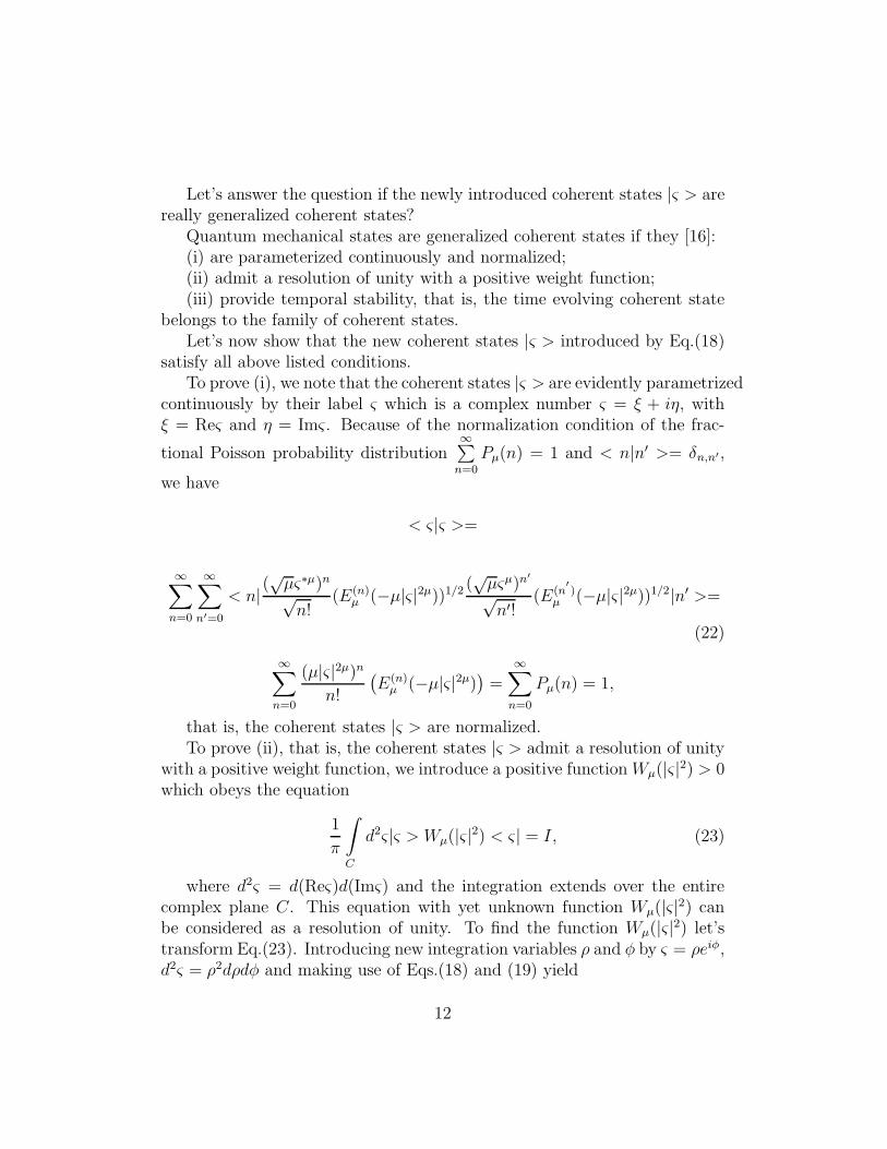
Let’s answer the question if the newly introduced coherent states |ς > arereally generalized coherent states?

Quantum mechanical states are generalized coherent states if they [16]:(i) are parameterized continuously and normalized;(ii) admit a resolution of unity with a positive weight function;(iii) provide temporal stability, that is, the time evolving coherent state

belongs to the family of coherent states.Let’s now show that the new coherent states |ς > introduced by Eq.(18)

satisfy all above listed conditions.To prove (i), we note that the coherent states |ς > are evidently parametrized

continuously by their label ς which is a complex number ς = ξ + iη, withξ = Reς and η = Imς . Because of the normalization condition of the frac-

tional Poisson probability distribution∞∑

n=0

Pµ(n) = 1 and < n|n′ >= δn,n′,

we have

< ς|ς >=

∞∑

n=0

∞∑

n′=0

< n|(√µς∗µ)n√n!

(E(n)µ (−µ|ς|2µ))1/2 (

√µςµ)n

′

√n′!

(E(n′

)µ (−µ|ς|2µ))1/2|n′ >=

(22)

∞∑

n=0

(µ|ς|2µ)nn!

(


)

=

∞∑

n=0

Pµ(n) = 1,

that is, the coherent states |ς > are normalized.To prove (ii), that is, the coherent states |ς > admit a resolution of unity

with a positive weight function, we introduce a positive functionWµ(|ς|2) > 0which obeys the equation

1

π

∫

C

d2ς|ς > Wµ(|ς|2) < ς | = I, (23)

where d2ς = d(Reς)d(Imς) and the integration extends over the entirecomplex plane C. This equation with yet unknown function Wµ(|ς|2) canbe considered as a resolution of unity. To find the function Wµ(|ς|2) let’stransform Eq.(23). Introducing new integration variables ρ and φ by ς = ρeiφ,d2ς = ρ2dρdφ and making use of Eqs.(18) and (19) yield

12

1

π

∫

C

d2ς|ς > Wµ(|ς|2) < ς| =

1

π

∞∑

n=0

∞∑

m=0

∞∫

0

dρρ(n+m)µ+1

2π∫

0

dφei(n−m)φWµ(ρ2)√

n!m!

(

E(n)µ (−µ|ρ|2µ)

)1/2× (24)

(

E(m)µ (−µ|ρ|2µ)

)1/2 |n >< m| = I.

By interchanging the orders of summation and integration and carryingout the integration over φ, we get a factor 2πδn,m, which reduces the doublesummation to a single one. Therefore, Eq.(24) is simplified to

1

π

∫

C

d2ς|ς > Wµ(|ς|2) < ς| =

∞∑

n=0

2

n!

∞∫

0

dρρ2nµ+1Wµ(ρ2)E(n)

µ (−µ|ρ|2µ)|n >< n| = I. (25)

Because of the completeness of orthonormal vectors |n >∞∑

n=0

|n >< n| = I, (26)

we come to the following integral equation to find the positive functionWµ(x)

∞∫

0

dxxµnWµ(x)E(n)µ (−µxµ) = n!. (27)

To solve Eq.(27) we use the Laplace transform of the function tµnE(n)µ (−µtµ),

see Appendix,

∞∫

0

dte−sttµnE(n)µ (−µtµ) = n! · sµ−1

(sµ + µ)n+1. (28)

13

By comparing Eqs.(27) and (28) we conclude that the positive functionWµ(x) has the form

Wµ(x) = (1− µ)1−µ

µ · exp{−(1− µ)1/µx}, 0 < µ ≤ 1. (29)

Thus, we proved that the coherent states |ς > admit a resolution of unitywith the positive weight functionWµ(x) given by Eq.(29). At µ = 1, functionWµ(x) becomes

W1(x) = limµ→1

Wµ(x) = limµ→1

[

(1− µ)1−µµ · exp{−(1− µ)1/µx}

]

= 1,

and we come back to the resolution of unity equation for the standardcoherent states |z >

1

π

∫

C

d2z|z >< z| = I. (30)

To prove (iii), we note that if |n > is an eigenvector of the HamiltonianH = ~ωN = ~ωa+a, where ~ is Planck’s constant, then the time evolutionoperator exp(−iHt/~) results

exp(−iHt/~)|n >= e−iωnt|n > .

In other words, the time evolution of |n > results in appearance of thephase factor only while the state does not change. Let’s consider time evo-lution of the coherent state |ς > defined by Eq.(18). Well, as far as thecoherent state is not an eigenstate of H then one may expect that it evolvesinto other states in time. However, it follows that

exp(−iHt/~)|ς >=∞∑

n=0

(√µςµ)n√n!

(E(n)µ (−µ|ς|2µ))1/2e−iωnt|n >= |e− iωt

µ ς >,

(31)which is just another coherent state belonging to a complex number

ςe−iωtµ . We see that the time evolution of the coherent state |ς > remains

within the family of coherent states |ς >. The property embodied in Eq.(31)is the temporal stability of coherent states |ς > under the action of H .

Thus, we conclude that the new coherent states |ς > satisfy the Klauder’scriteria set (i) - (iii) for generalized coherent states.

14

Finally, let us introduce an alternative notation for |ς > in terms of thereal ξ and imaginary η parts of |ς >, that is, |ς >= |ξ + iη > /

√2~. Then

from Eq.(18) we have

|ς >= |ξ, η >=∞∑

n=0

(√µ(ξ + iη)µ)n√

(2~)nµn!(E(n)

µ (−µ(

ξ2 + η2

2~

)µ

))1/2|n > . (32)

The adjoint coherent states are defined as

< ς | =< ξ, η| =∞∑

n=0

< n|(√µ(ξ − iη)µ)n√

(2~)nµn!(E(n)

µ (−µ(

ξ2 + η2

2~

)µ

))1/2. (33)

Despite the fact that the adjoint state is labelled by ς , the series expansionEq.(33) are formed in fact of powers of ς∗.

3.1 Quantum mechanical vector and operator repre-

sentations based on coherent states |ς >In spirit of Klauder’s consideration [24], let’s show that the resolution of unitycriteria Eq.(23) with Wµ(x) given by Eq.(29) allows us to list fundamentalquantum mechanical statements pertaining to the associated representationof Hilbert space. Indeed, it is easy to see that the newly introduced coherentstates |ς > provide:

1. Inner Product of quantum mechanical vectors |ϕ > and |ψ > definedas

< ϕ|ψ >= 1

π

∫

C

d2ς < ϕ|ς > Wµ(|ς|2) < ς|ψ >, (34)

where d2ς = d(Reς)d(Imς) and the integration extends over the entirecomplex plane C, weight function Wµ(x) is defined by Eq.(29), the vectorrepresentatives are wave functions < ϕ|ς > and < ς|ψ > given by

< ϕ|ς >=∞∑

n=0

(√µςµ)n√n!

(E(n)µ (−µ|ς|2µ))1/2 < ϕ|n >, (35)

< ς|ψ >=∞∑

n=0

< n|ψ > (√µς∗µ)n√n!

(E(n)µ (−µ|ς|2µ))1/2. (36)

15

2. Vectors Transformation Law

< ς |A|ψ >= 1

π

∫

C

d2ς′

< ς|A|ς ′ > Wµ(|ς′ |2) < ς

′ |ψ >, (37)

where < ς|A|ς ′ > is the matrix element of quantum mechanical operatorA.

3. Operator Transformation Law

< ς|A1A2|ς′

>=1

π

∫

C

d2ς′′

< ς|A1|ς′′

> Wµ(|ς′′ |2) < ς

′′|A2|ς′

>, (38)

where A1 and A2 are two quantum mechanical operators.Further, the inverse map from the functional Hilbert space representation

of coherent states |ς > to the abstract one is provided by the followingdecomposition laws:

4. Vector Decomposition Law

|ψ >= 1

π

∫

C

d2ς |ς > Wµ(|ς|2) < ς |ψ > . (39)

5. Operator Decomposition Law

A =1

π

∫

C

d2ς1d2ς2 |ς1 > Wµ(|ς1|2) < ς1|A|ς2 > Wµ(|ς2|2) < ς2|. (40)

Thus, we conclude that the resolution of unity Eq.(23) with Wµ(x), givenby Eq.(29), provides an appropriate inner product Eq.(34) and lets us intro-duce the Hilbert space, Eqs.(37) - (40).

All of the above listed results lead to the well-know fundamental equationsof quantum optics and coherent states theory [24], [25] in the limit case µ = 1.

Table 2 summarizes the definitions and equations attributed to the newlyintroduced coherent states |ς > with those for the coherent states |z >. Table2 presents two sets of equations for a coherent state |... >, for an adjointcoherent state <...|, for the probability P (n) that n photons will be found inthe coherent state |... >, for a positive weight functionW (x) in the resolutionof unity equations (23) and (30), the mean number < ...|a+a|... > of photons

16

when the state is a coherent state |... >, and the quantum mechanical vectordecomposition law.

|ς > (0 < µ ≤ 1) |z >|... >

∞∑

n=0

(√µςµ)n√n!

(E(n)µ (−µ|ς|2µ))1/2|n > e−

12|z|2

∞∑

n=0

zn√n!|n >

<...|∞∑

n=0

< n| (√µς∗µ)n√n!

(E(n)µ (−µ|ς|2µ))1/2 <n|e− 1

2|z|2

∞∑

n=0

z∗n√n!

P (n) (µ|ς|2µ)nn!

E(n)µ (−µ|ς|2µ) |z|2n

n!e−|z|2

W (x) (1− µ)1−µ

µ · exp{−(1− µ)1µx} 1

< ...|a+a|... > (µ|ς|2µ)/Γ(µ+ 1) |z|2|ψ > 1

π

∫

C

d2ς|ς > Wµ(|ς|2) < ς|ψ > 1π

∫

C

d2z|z >< z|ψ >

Table 2. Coherent states |ς > vs coherent states |z >.

4 Generalized Bell and Stirling Numbers

4.1 Fractional Bell polynomials and fractional Bell num-

bers

Based on the fractional Poisson probability distribution Eq.(9) we introducea new generalization of the Bell polynomials

Bµ(x,m) =∞∑

n=0

nmxn

n!

∞∑

k=0

(k + n)!

k!

(−x)kΓ(µ(k + n) + 1)

, Bµ(x, 0) = 1, (41)

where the parameter µ is 0 < µ ≤ 1.We will callBµ(x,m) as the fractionalBell polynomials of m-order. A few fractional Bell polynomials are

Bµ(x, 1) =x

Γ(µ+ 1), (42)

Bµ(x, 2) =2x2

Γ(2µ+ 1)+

x

Γ(µ+ 1), (43)

Bµ(x, 3) =6x3

Γ(3µ+ 1)+

6x2

Γ(2µ+ 1)+

x

Γ(µ+ 1), (44)

17

Bµ(x, 4) =24x4

Γ(4µ+ 1)+

36x3

Γ(3µ+ 1)+

14x2

Γ(2µ+ 1)+

x

Γ(µ+ 1). (45)

The polynomials Bµ(x,m) are related to the well-known Bell polynomials[17] B(x,m) by

Bµ(x,m)|µ=1 = B(x,m) = e−x

∞∑

n=0

nmxn

n!. (46)

From Eq.(41) at x = 1 we come to a new numbers Bµ(m), which we callthe fractional Bell numbers

Bµ(m) = Bµ(x,m)|x=1 =∞∑

n=0

nm

n!

∞∑

k=0

(k + n)!

k!

(−1)k

Γ(µ(k + n) + 1). (47)

As an example, here are a few fractional Bell numbers

Bµ(0) = 1, Bµ(1) =1

Γ(µ+ 1), Bµ(2) =

2

Γ(2µ+ 1)+

1

Γ(µ+ 1),

Bµ(3) =6

Γ(3µ+ 1)+

6

Γ(2µ+ 1)+

1

Γ(µ+ 1),

Bµ(4) =24

Γ(4µ+ 1)+

36

Γ(3µ+ 1)+

14

Γ(2µ+ 1)+

1

Γ(µ+ 1).

It is easy to see that Eq.(47) can be written as

Bµ(m) =∞∑

n=0

nm

n!E(n)

µ (−1), (48)

where E(n)µ (−1) = (dnEµ(z)/dz

n)|z=−1 and Eµ(z) is given by Eq.(8). Thenew formula Eq.(48) is in fact a fractional generalization of so-called Dobinskirelation known since 1877 [21], [22]. Indeed, at µ = 1 when the Mittag-Leffler function is just the exponential function, E1(z) = exp(z), we have,

E(n)1 (−1) = (dnE1(z)/dz

n)|z=−1 = e−1, and the equation (48) becomes theDobinski relation [21] for the Bell numbers B(m),

18

B(m) = Bµ(m)|µ=1 = e−1∞∑

n=0

nm

n!. (49)

Now we focus on the general definitions given by Eqs.(41) and (48) tofind the generating functions of the polynomials Bµ(x,m) and the numbersBµ(m). Let us introduce the generating function of the polynomials Bµ(x,m)as

Fµ(s, x) =∞∑

m=0

sm

m!Bµ(x,m). (50)

Therefore, to get the polynomial Bµ(x,m) we should differentiate Fµ(s, x)m times with respect to s, and then let s = 0. That is,

Bµ(x,m) =∂m

∂smFµ(s, x)|s=0. (51)

To find an explicit equation for Fµ(s, x), let’s substitute Eq.(41) intoEq.(50) and evaluate the sum over m. As a result we have

Fµ(s, x) =∞∑

n=0

xn

n!esn

∞∑

k=0

(k + n)!

k!

(−x)kΓ(µ(k + n) + 1)

. (52)

Then, introducing the new summation variable l = k + n, yields

Fµ(s, x) =∞∑

n=0

xn

n!esn

∞∑

l=n

l!

(l − n)!

(−x)l−n

Γ(µl + 1)=

∞∑

l=0

1

Γ(µl + 1)

l∑

n=0

l!

n!(l − n)!esnxn(−x)l−n =

∞∑

l=0

(xes − x)l

Γ(µl + 1).

Finally, we obtain

Fµ(s, x) = Eµ(x(es − 1)), (53)

where Eµ(z) is the Mittag-Leffler function defined by the power seriesEq.(8).

Thus, we have

Eµ(x(es − 1)) =

∞∑

m=0

sm

m!Bµ(x,m). (54)

19

It is easy to see that the generating function Fµ(s, x), given by Eq.(53),can be considered as the moment generating function of the fractional Poissonprobability distribution (see Eq.(35) in Ref.[9]).

In the case of µ = 1, Eq.(53) turns into the equation for the generatingfunction of the Bell polynomials B(x,m) defined by Eq.(46),

F1(s, x) = exp{x(es − 1)} =∞∑

m=0

sm

m!B(x,m). (55)

If we put x = 1 in Eq.(53), then we immediately come to the generatingfunction Bµ(s) of the fractional Bell numbers Bµ(m)

Bµ(s) =∞∑

m=0

sm

m!Bµ(m) = Eµ(e

s − 1). (56)

The numbers Bµ(m) can be obtained by differentiating Bµ(s) m timeswith respect to s, and then letting s = 0,

Bµ(m) =∂m

∂smBµ(s, x)|s=0. (57)

When µ = 1, Eq.(56) reads

B1(s) =

∞∑

m=0

sm

m!B1(m) = exp(es − 1), (58)

and we come to the well-known equation for the generating function ofthe Bell numbers.

Now we are going to consider quantum physics and probability theoryproblems where the fractional Bell polynomials appear.

4.1.1 Quantum physics application of the fractional Bell polyno-

mials

As quantum physics applications of the fractional Bell polynomials let usshow how the fractional Bell polynomials are related to the new coherentstates |ς > introduced by Eq.(18). For the boson creation a+ and a anni-hilation operators of a photon field that satisfy the commutation relation[a, a+] = aa+ − a+a = 1, the diagonal matrix element of the n-th power ofthe number operator (a+a)n yields the fractional Bell polynomials of ordern,

20

< ς|(a+a)n|ς >= Bµ(|ς|2µ, n). (59)

Then, the diagonal coherent state |ς >matrix element < ς | exp(−iHt/~)|ς >of the time evolution operator

exp(−iHt/~) = exp{

(−iωt/~)a+a}

(60)

can be written as

< ς| exp{

(−iωt/~)a+a}

|ς >=∞∑

n=0

1

n!(−iωt

~)n < ς|(a+a)n|ς >= (61)

∞∑

n=0

1

n!(−iωt

~)nBµ(|ς|2µ, n),

where ~ is Planck’s constant. By comparing with Eq.(50) we concludethat

< ς| exp{

(−iωt/~)a+a}

|ς >= Eµ

(

|ς|2µ(exp(−iωt/~)− 1))

. (62)

In other words, the diagonal coherent state |ς > matrix element of theoperator exp {(−iωt/~)a+a} is the generating function of the fractional Bellpolynomials. In the special case µ = 1, Eq.(62) reads

< z| exp{

(−iωt/~)a+a}

|z >= exp{|z|2(exp(−iωt/~)− 1)}, (63)

that is, the diagonal coherent state |z > matrix element of the operatorexp {(−iωt/~)a+a} is the generating function of the Bell polynomials. Thisstatement immediately follows from Eqs.(11.5-2) and (11.2-10) of Ref.[26] forthe diagonal matrix element of the operator exp {(−iωt/~)a+a} in the basisof the coherent states |z >.

It follows from Eq.(59) that for the special case when |ς| = 1 the diagonalmatrix element of the n-th power of the number operator (a+a)n yields thefractional Bell number of order n,

< ς|(a+a)n|ς > ||ς|=1 = Bµ(|ς|2µ, n)||ς|=1 = Bµ(n). (64)

21

At µ = 1 this equation turns into the relationship between the well-knownBell numbers B(n) and the diagonal matrix element of the n-th power of thenumber operator (a+a)n in the basis of the standard coherent states |z >,

< z|(a+a)n|z > ||z|=1 = B(|z|2µ, n)||z|=1 = B(n). (65)

The equation (65) originally was obtained in [35].

4.1.2 Fractional compound Poisson processes

As another example where the fractional Bell polynomials come from, weconsider the fractional compound Poisson process first introduced into theprobability theory and developed by Laskin in [9]. Let us consider the pair{N(t), Yi}, where {N(t), t ≥ 0]} is a counting Poisson process with a proba-bility distribution function P (n, t) and {Yi, i = 1, 2, ...} is a family of indepen-dent and identically distributed discrete random variables with probabilitydistribution function p(Y ) for each Yi. The process {N(t), t ≥ 0} and the se-quence {Yi, i = 1, 2, ...} are assumed to be independent. To be more specificwe will distinguish the following four cases:

1. In the pair {N(t), Yi} the counting process N(t) is the fractionalPoisson process with probability distribution function given by Eq.(9) andYi are random variables with the fractional Poisson probability distribution,that is the probability that Y = n has a form

p(Y = n) =(λµ)

n

n!

∞∑

k=0

(k + n)!

k!

(−λµ)k

Γ(µ(k + n) + 1), 0 < µ ≤ 1, (66)

where λµ is the parameter associated with random variable Y .2. In the pair {N(t), Yi} the counting process N(t) is the fractional

Poisson process with probability distribution function given by Eq.(9) andYi are random variables with the Poisson probability distribution, that is theprobability that Y = n has a form

p(Y = n) =(λ)n

n!e−λ. (67)

3. In the pair {N(t), Yi} the counting process N(t) is the Poisson pro-cess with probability distribution function given by Eq.(12) and Yi are ran-dom variables with the fractional Poisson probability distribution, that is theprobability that random variable Y = n is given by Eq.(66).

22

4. In the pair {N(t), Yi} the counting process N(t) is the Poisson processwith probability distribution function given by Eq.(12) and Yi are randomvariables with the Poisson probability distribution, that is the probabilitythat Y = n is given by Eq.(67).

The compound Poisson process X(t) is represented by

X(t) =

N(t)∑

i=1

Yi. (68)

The moment generating function Jµ(s, t) of compound Poisson processhas been introduced as [9]

Jµ(s, t) =< exp{sX(t)} >N(t),Yi, (69)

where < ... >N(t),Yistands for two statistically independent averaging

procedures:a). Averaging over random number n governed by the counting Poisson

process

< ... >N(t)=

∞∑

n=0

P (n, t)..., (70)

where P (n, t) is given either by Eq.(9) or by Eq.(12).b). Averaging over independent random variables Yi, < ... >Yi

< ... >Yi=

∫

dY1...dYnp(Y1)...p(Yn)..., (71)

where p(Yi) is the probability density of random variable Yi given eitherby Eq.(66) or by Eq.(67).

To obtain equation for the moment generating function Jµ(s, t) we applyEqs.(70) and (71) to Eq.(69),

Jµ(s, t) =

∞∑

n=0

Pµ(n, t) < exp{sX(t)|N(t) = n} >Yi=

∞∑

n=0

< exp{s(Y1 + ...+ Yn)} >Yi×(νtµ)n

n!

∞∑

k=0

(k + n)!

k!

(−νtµ)kΓ(µ(k + n) + 1)

=

(72)

23

∞∑

n=0

< exp{s(Y1)} >nYi×(νtµ)n

n!

∞∑

k=0

(k + n)!

k!

(−νtµ)kΓ(µ(k + n) + 1)

,

where we used the independence between N(t) and {Y1, Y2, ...}, and theindependence of the Yi’s between themselves. Hence, letting

g(s) =< esY >Y , (73)

for the moment generating function of random variables Yi, we find fromEq.(72) the moment generating function Jµ(s, t) of the fractional compoundPoisson process

Jµ(s, t) =∞∑

n=0

gn(s)×(νtµ)n

n!

∞∑

k=0

(k + n)!

k!

(−νtµ)kΓ(µ(k + n) + 1)

= Eµ(νtµ(g(s)−1)).

(74)It follows from Eq.(69) that kth order moment of fractional compound

Poisson process X(t) is obtained by differentiating Jµ(s, t) k times with re-spect to s, then putting s = 0, that is

< Xk(t) >N(t),Yi=

∂k

∂skJµ(s, t)|s=0. (75)

For the case 1, when N(t) is the fractional Poisson process and Yi arerandom variables with the fractional Poisson probability distribution, weobtain

J (1)µ (s, t) = Eµ(νt

µ(g1(s)− 1)), (76)

with

g1(s) =< esY >Yi= Eµ(λµ(e

s − 1)). (77)

Thus, we have

J (1)µ (s, t) = Eµ(νt

µ{Eµ(λµ(es − 1))− 1}). (78)

For the case 2, when N(t) is the fractional Poisson process and Yi arerandom variables with the Poisson probability distribution, we obtain

J (2)µ (s, t) = Eµ(νt

µ(g2(s)− 1)), (79)

24

with

g2(s) =< esY >Yi= exp(λ(es − 1)). (80)

Thus, we have

J (2)µ (s, t) = Eµ(νt

µ{exp(λ(es − 1))− 1}). (81)

For the case 3, when N(t) is the fractional Poisson process and Yi arerandom variables with the fractional Poisson probability distribution, weobtain

J (3)µ (s, t) = exp(νt(g3(s)− 1)), (82)

with

g3(s) =< esY >Yi= Eµ(λµ(e

s − 1)). (83)

and the parameter ν comes from Eq.(12).Thus, we have

J (3)µ (s, t) = exp(νt{Eµ(λµ(e

s − 1))− 1}). (84)

For the case 4, when N(t) is the Poisson process and Yi are randomvariables with the Poisson probability distribution, we obtain

J (4)(s, t) = exp(νt(g4(s)− 1)), (85)

with

g4(s) =< esY >Yi= exp(λ(es − 1)). (86)

Thus, we have

J (4)(s, t) = exp(νt{exp(λ(es − 1))− 1}). (87)

Now, let us take a look at the moment generating function J(2)µ (s, t) given

by Eq.(81). It can be expanded as

J (2)µ (s, t) =

∞∑

m=0

(λ(es − 1))m

m!Bµ(νt

µ, m) = (88)

25

∞∑

m=0

λm∞∑

k=m

sk

k!S(k,m)Bµ(νt

µ, m). (89)

where we used Eqs (54) and (122). Finally, we have for J(2)µ (s, t),

J (2)µ (s, t) = Eµ(νt

µ{exp(λ(es − 1))− 1}) =∞∑

k=0

sk

k!

k∑

m=0

λmS(k,m)Bµ(νtµ, m).

(90)Then as it follows from Eq.(75) that kth order moment of fractional com-

pound Poisson process for the case 2 is

< Xk(t) >(2)N(t),Yi

=∂k

∂skJ (2)µ (s, t)|s=0 =

k∑

m=1

λmS(k,m)Bµ(νtµ, m), (91)

where S(k,m) are the standard Stirling numbers of the second kind andBµ(νt

µ, m) are the fractional Bell polynomials defined by Eq.(41).Thus, this example shows the way the fractional Bell polynomials appear,

if one evaluates moments of fractional compound Poisson process for the case2.

It is easy to see that when µ = 1, the case 2 turns into the case 4. Hence,at µ = 1 for the moment generating function J (4)(s, t) we have

J (4)(s, t) =

∞∑

k=0

sk

k!

k∑

m=0

λmS(k,m)B(νt,m), (92)

and kth order moment of compound Poisson process for the case 4 is

< Xk(t) >(4)N(t),Yi

=∂k

∂skJ (4)(s, t)|s=0 =

k∑

m=1

λmS(k,m)B(νt,m), (93)

where B(νtµ, m) are the Bell polynomials defined by Eq.(46).The first two moments of fractional compound Poisson process for the

case 2 are

26

< X1(t) >(2)N(t),Yi

=∂

∂sJ (2)µ (s, t)|s=0 = λS(1, 1)Bµ(νt

µ, 1) = λνtµ

Γ(µ+ 1), (94)

< X2(t) >(2)N(t),Yi

=∂2

∂s2J (2)µ (s, t)|s=0 =

2∑

m=1

λmS(2, m)Bµ(νtµ, m), (95)

Equation (94) for the first order moment of fractional Poisson process wasfound at first time in [9]. Using expressions for fractional Bell polynomialsBµ(νt

µ, 1) and Bµ(νtµ, 2) yields

< X2(t) >(2)N(t),Yi

= λ2(

2(νtµ)2

Γ(2µ+ 1)+

νtµ

Γ(µ+ 1)

)

+ λνtµ

Γ(µ+ 1). (96)

with S(2, 1) = 1 and S(2, 2) = 1.

Then, the variance σ(2)N(t),Yi

for the case 2 is

σ(2)N(t),Yi

=(

< X2(t) >(2)N(t),Yi

−(< X1(t) >(2)N(t),Yi

)2)

=

λ2(

2(νtµ)2

Γ(2µ+ 1)+

νtµ

Γ(µ+ 1)

)

+ λνtµ

Γ(µ+ 1)−(

λνtµ

Γ(µ+ 1)

)2

.

Or, after simple transformations (see, for instance, page 207 in [9]) wehave

σ(2)N(t),Yi

= λ2(

µB(µ, 12)

2µ−1− 1

)(

νtµ

Γ(µ+ 1)

)2

+ (λ2 + λ)νtµ

Γ(µ+ 1), (97)

where B(µ, 12) is the Beta-function defined as[36]

B(µ, ν) =Γ(µ)Γ(ν)

Γ(µ+ ν). (98)

At µ = 1 Eqs.(94) and (95) are transformed into the first two momentsof compound Poisson process for the case 4,

27

< X1(t) >(4)N(t),Yi

=∂

∂sJ (4)(s, t)|s=0 = λS(1, 1)B(νt, 1) = λνt, (99)

< X2(t) >(4)N(t),Yi

=∂2

∂s2J (4)(s, t)|s=0 =

2∑

m=1

λmS(2, m)B(νt,m) = (100)

λ2(νt)2 + (λ2 + λ)νt.

Then the variance σ(4)N(t),Yi

for the case 4 is

σ(4)N(t),Yi

=(

< X2(t) >(4)N(t),Yi

−(< X1(t) >(4)N(t),Yi

)2)

= (λ2 + λ)νt. (101)

We see, that Eq.(101) follows straighforwardly from Eq.(97) at µ = 1with substitution ν → ν.

The Table 3 displays the moment generating functions for each of fourcases introduced above.

N(t), 0 < µ < 1 N(t), µ = 1

Yi, 0 < µ < 1Case 1

Eµ(νtµ{Eµ(λµ(e

s−1))−1})Case 3

exp (νt{Eµ(λµ(es−1))−1})

Yi, µ = 1Case 2

Eµ(νtµ{ exp (λ(es−1))−1})

Case 4

exp (νt{ exp (λ(es−1))−1})

Table 3. The moment generating functions of fractional compound Pois-

son processes.

4.2 Fractional Stirling numbers of the second kind

We introduce the fractional generalization of the Stirling numbers4 of thesecond kind Sµ(m, l) by means of equation

Bµ(x,m) =m∑

l=0

Sµ(m, l)xl, (102)

4Stirling numbers, introduced by J. Stirling [18] in 1730, have been studied in thepast by many celebrated mathematicians. Among them are Euler, Lagrange, Laplaceand Cauchy. Stirling numbers play an important role in combinatorics, number theory,probability and statistics. There are two common sets of Stirling numbers, they are so-called Stirling numbers of the first kind and Stirling numbers of the second kind (fordetails, see Refs.[19], [20]).

28

where Bµ(x,m) is a fractional generalization of the Bell polynomials givenby Eq.(41) and the parameter µ is 0 < µ ≤ 1. At µ = 1, Eq.(102) definesthe integers S(m, l) = Sµ(m, l)|µ=1, which are called Stirling numbers ofthe second kind. At x = 1, when the fractional Bell polynomials Bµ(x,m)become the fractional Bell numbers, Bµ(m) = Bµ(x,m)|x=1, Eq.(102) givesus a new equation to express fractional Bell numbers in terms of fractionalStirling numbers of the second kind

Bµ(m) =

m∑

l=0

Sµ(m, l). (103)

To find Sµ(m, l) we transform the right-hand side of Eq.(41) as follows

Bµ(x,m) =∞∑

n=0

nmxn

n!

∞∑

k=0

(k + n)!

k!

(−x)kΓ(µ(k + n) + 1)

=

∞∑

n=0

nmxn

n!

∞∑

l=0

θ(l − n)l!

(l − n)!

(−x)l−n

Γ(µl + 1), (104)

here θ(l) is the Heaviside step function,

θ(l) =| 1, if l ≥ 0

0, if l < 0. (105)

Then, interchanging the order of summations in Eq.(104) yields

Bµ(x,m) =

∞∑

l=0

xl

Γ(µl + 1)

l∑

n=0

nm (−1)l−nl!

n!(l − n)!=

∞∑

l=0

xl

Γ(µl + 1)

l∑

n=0

(−1)l−n

(

l

n

)

nm,

(106)where the notation

(

ln

)

= l!n!(l−n)!

has been introduced.

By comparing Eq.(102) and Eq.(106) we conclude that the fractionalStirling numbers Sµ(m, l) are given by

Sµ(m, l) =1

Γ(µl + 1)

l∑

n=0

(−1)l−n

(

l

n

)

nm, (107)

Sµ(m, 0) = δm,0, Sµ(m, l) = 0, l = m+ 1, m+ 2, ....

29

As an example, Table 4 presents a few of fractional Stirling numbers ofthe second kind.

m\l 1 2 3 4 5 6 71 1

Γ(µ+1)

2 1Γ(µ+1)

2Γ(2µ+1)

3 1Γ(µ+1)

6Γ(2µ+1)

6Γ(3µ+1)

4 1Γ(µ+1)

14Γ(2µ+1)

36Γ(3µ+1)

24Γ(4µ+1)

5 1Γ(µ+1)

30Γ(2µ+1)

150Γ(3µ+1)

240Γ(4µ+1)

120Γ(5µ+1)

6 1Γ(µ+1)

62Γ(2µ+1)

540Γ(3µ+1)

1560Γ(4µ+1)

1800Γ(5µ+1)

720Γ(6µ+1)

7 1Γ(µ+1)

126Γ(2µ+1)

1806Γ(3µ+1)

8400Γ(4µ+1)

16800Γ(5µ+1)

15120Γ(6µ+1)

5040Γ(7µ+1)

Table 4. Fractional Stirling numbers of the second kind Sµ(m, l) (0 <µ ≤ 1).

Some special cases are

Sµ(m, 1) =1

Γ(µ+ 1), Sµ(m, 2) = (2m−1 − 1)

2

Γ(2µ+ 1), (108)

Sµ(m, 3) = (3m − 3 · 2m + 3)1

Γ(3µ+ 1), (109)

Sµ(m, 4) = (4m − 4 · 3m + 6 · 2m − 4)1

Γ(4µ+ 1), (110)

Sµ(m,m− 1) =m! · (m− 1)

2Γ((m− 1)µ+ 1), Sµ(m,m) =

m!

Γ(mµ+ 1). (111)

It is easy to see that at µ = 1 Eq.(107) turns into the well known represen-tation for the standard Stirling numbers S(m, l) = Sµ(m, l)|µ=1 ≡ S1(m, l)of the second kind [37],

S(m, l) =1

l!

l∑

n=0

(−1)l−n

(

l

n

)

nm.

Thus, one can conclude that there is a relationship between fractionalStirling numbers Sµ(m, l) of the second kind and standard Stirling numbersS(m, l) of the second kind

30

Sµ(m, l) =l!

Γ(µl + 1)S(m, l). (112)

or

S(m, l) =Γ(µl + 1)

l!Sµ(m, l). (113)

Let’s note that Eqs.(112) or (113) allow us to find new equations andidentities for the fractional Stirling numbers Sµ(m, l) based on the well-knowequations and identities for the standard Stirling numbers S(m, l) of thesecond kind. For example, considering the recurrence relation for Stirlingnumbers of the second kind [37], (see, page 825)

S(m+ 1, l) = lS(m, l) + S(m, l − 1),

and using Eq.(112) yield the new recurrence relation for fractional Stirlingnumbers Sµ(m, l) of the second kind

Sµ(m+ 1, l) = lSµ(m, l) + lΓ(µ(l − 1) + 1)

Γ(µl + 1)Sµ(m, l − 1). (114)

To find a generating function of the fractional Stirling numbers Sµ(m, l)of the second kind, let’s expand the generating function Fµ(s, x) given byEq.(50). Upon substituting Bµ(x,m) from Eq.(102) we have the followingchain of transformations

Fµ(s, x) =

∞∑

m=0

sm

m!

(

m∑

l=0

Sµ(m, l)xl

)

=

∞∑

m=0

sm

m!

( ∞∑

l=0

θ(m− l)Sµ(m, l)xl

)

=

∞∑

l=0

( ∞∑

m=l

Sµ(m, l)sm

m!

)

xl, (115)

where θ(m− l) is the Heaviside step function defined by Eq.(105).On the other hand, from Eq.(53), we have for Fµ(s, x)

Fµ(s, x) =∞∑

l=0

(es − 1)l

Γ(µl + 1)xl. (116)

31

Upon comparing this equation and Eq.(115), we conclude that

∞∑

m=l

Sµ(m, l)sm

m!=

(es − 1)l

Γ(µl + 1), l = 0, 1, 2, .... (117)

Now we are set up to introduce two generating functions Gµ(s, l) andFµ(s, t) of the fractional Stirling numbers of the second kind,

Gµ(s, l) =∞∑

m=l

Sµ(m, l)sm

m!=

(es − 1)l

Γ(µl + 1), (118)

Fµ(s, t) =∞∑

m=0

m∑

l=0

Sµ(m, l)smtl

m!=

∞∑

l=0

tl(es − 1)l

Γ(µl + 1)= Eµ(t(e

s − 1)). (119)

Hence, it follows from Eq.(118) that

Sµ(m, l) =∂mGµ(s, l)

∂sm|s=0 =

1

Γ(µl + 1)

∂m

∂sm(es − 1)l|s=0, (120)

and from Eq.(119) we have for Sµ(m, l)

Sµ(m, l) =1

l!

∂m+lFµ(s, t)

∂sm∂tl|s=0,t=0 =

1

l!

∂m+l

∂sm∂tlEµ(t(e

s−1))|s=0,t=0, l ≤ m.

(121)As a special case µ = 1, equations (118) and (119) include the well-know

generating function equations for the standard Stirling numbers of the secondkind S(m, l) (for instance, see Eqs.(2.17) and (2.18) in Ref.[20]),

G1(s, l) = Gµ(s, l) |µ=1=∞∑

m=l

S(m, l)sm

m!=

(es − 1)l

l!, l = 0, 1, 2, .... (122)

and

F1(s, t) = Fµ(s, t) |µ=1=

∞∑

m=0

m∑

l=0

S(m, l)smtl

m!= exp(t(es − 1)). (123)

To get some insight on where fractional Stirling numbers of the secondkind may come from, let us prove the following lemma.

32

Lemma:

If the function Aµ(s) can be presented by the series expansion

Aµ(s) =∞∑

l=0

alsl

Γ(µl + 1), 0 < µ ≤ 1, (124)

then

Aµ(es − 1) =

∞∑

m=0

bmsm

m!, 0 < µ ≤ 1. (125)

where numbers bm are related to the numbers al by means of the rela-tionship

bm =

m∑

l=0

Sµ(m, l)al, (126)

with Sµ(m, l) are being fractional Stirling numbers of the second kindintroduced by Eq.(107).

Proof.

Upon substituting es − 1 instead of s into Eq.(124) we have the followingchain of transformations

Aµ(es − 1) =

∞∑

l=0

al(es − 1)l

Γ(µl + 1)=

∞∑

l=0

alΓ(µl + 1)

l∑

k=0

(−1)l−k

(

l

k

) ∞∑

m=0

(sk)m

m!=

∞∑

m=0

sm

m!

m∑

l=0

alΓ(µl + 1)

l∑

k=0

(−1)l−k

(

l

k

)

km =∞∑

n=0

bmsm

m!,

where bm is given by Eq.(126), with Sµ(m, l) defined by Eq.(107) and thecondition Sµ(m, l) = 0, l ≥ m+ 1 has been taken into account.

Thus, we proved the lemma.Table 5 summarizes equations for the Bell polynomials B(x,m), the Bell

numbers B(m), the Stirling numbers of the second kind S(m, l), the m-thorder moment nm, generating function of the Stirling numbers of the second

kind∞∑

m=l

Sµ(m, l)sm/m!, and generating function B(s) of the Bell numbers,

attributed to the fractional Poisson distribution with those for the standardPoisson distribution.

33

fractional Poisson (0 < µ ≤ 1) Poisson (µ = 1)

B(x,m)∞∑

n=0

nmxn

n!

∞∑

k=0

(k+n)!k!

(−x)k

Γ(µ(k+n)+1)e−x

∞∑

n=0

nmxn

n!

B(m)∞∑

n=0

nm

n!E

(n)µ (−1) e−x

∞∑

n=0

nm

n!

S(m, l) 1Γ(µl+1)

l∑

n=0

(−1)l−n(

ln

)

nm 1l!

l∑

n=0

(−1)l−n(

ln

)

nm

nmm∑

l=0

Sµ(m, l)(νtµ)l

m∑

l=0

S(m, l)(νt)l

∞∑

m=l

Sµ(m, l)sm

m!(es−1)l

Γ(µl+1)(es−1)l

l!

B(s) Eµ(es − 1) exp(es − 1)

Table 5. Polynomials, numbers, moments and generating functions at-

tributed to the fractional Poisson process vs the standard Poisson process

4.2.1 A new representation for the Mittag-Leffler function

To obtain a new representation for the Mittag-Leffler function defined byEq.(8) we use the generating function of the Stirling numbers of the firstkind5

(1 + t)n =∞∑

m=0

tm

m!

m∑

l=0

s(m, l)nl, (128)

where s(m, l) stands for the Stirling numbers of the first kind [38].Then, we evaluate expectations of both sides of Eq.(128)

∞∑

n=0

Pµ(n, λ)(1 + t)n =∞∑

n=0

Pµ(n, λ)∞∑

m=0

tm

m!

m∑

l=0

s(m, l)nl, (129)

with fractional Poisson probability distribution Pµ(n, λ)

5The Stirling numbers of the first kind are defined as the coefficients s(m, l) in theexpansion

x!

(x−m)!= x(x − 1)...(x−m+ 1) =

m∑

l=0

s(m, l)xl. (127)

34

Pµ(n, λ) =(λ)n

n!

∞∑

k=0

(k + n)!

k!

(−λ)kΓ(µ(k + n) + 1)

, 0 < µ ≤ 1. (130)

Calculation on a left side of Eq.(129) results in Eµ(λt) and we have

Eµ(λt) =

∞∑

n=0

Pµ(n, λ)

∞∑

m=0

tm

m!

m∑

l=0

s(m, l)nl. (131)

Therefore, we come to the new representation for the Mittag-Leffler func-tion,

Eµ(λt) =

∞∑

m=0

tm

m!

m∑

l=0

s(m, l)Bµ(λ, l), (132)

where Eµ(λt) is the Mittag-Leffler function, s(m, l) are the Stirling num-bers of the first kind and Bµ(λ, l) are fractional Bell polynomials introducedby Eq.(41).

It is easy to see, that Eq.(132) can be written as

Eµ(λt) =

∞∑

m=0

tm

m!

m∑

l=0

s(m, l)

l∑

r=0

Sµ(l, r)λr, (133)

where the representation (102) of fractional Bell polynomials in terms offractional Stirling numbers of the second kind Sµ(l, r) has been used. Thelast equation can be written as

Eµ(λt) =∞∑

m=0

cm(µ, λ)tm

m!, (134)

if we introduce coefficients cm(µ, λ)

cm(µ, λ) =

m∑

l=0

s(m, l)Bµ(λ, l) =

m∑

l=0

s(m, l)

l∑

r=0

Sµ(l, r)λr. (135)

We see from Eq.(132) that the Mittag-Leffler function Eµ(λt) can be

considered as generating function to evaluate the summ∑

l=0

s(m, l)Bµ(λ, l), that

is

35

m∑

l=0

s(m, l)Bµ(λ, l) =∂m

∂tmEµ(λt)|t=0, (136)

or

m∑

l=0

s(m, l)l∑

r=0

Sµ(l, r)λr =

∂m

∂tmEµ(λt)|t=0. (137)

The new formulas (132)-(134) present the Mittag-Leffler function Eµ(λt)in terms of the Stirling numbers of the first kind s(m, l) and either fractionalBell polynomials Bµ(λ, l) or fractional Stirling numbers of the second kindSµ(l, r).

Comparing Eq.(8) and Eq.(132) yields two new identities

m∑

l=0

s(m, l)Bµ(λ, l) =m!

Γ(µm+ 1)λm, (138)

and

m∑

l=0

s(m, l)

l∑

r=0

Sµ(l, r)λr =

m!

Γ(µm+ 1)λm, (139)

where Eq.(102) has been taken into account.At the limit case µ = 1 we have from these two equations

m∑

l=0

s(m, l)B(λ, l) = λm, (140)

or

m∑

l=0

s(m, l)l∑

r=0

S(l, r)λr = λm. (141)

Hence, Eqs.(132)-(134) are transformed into the series expansion for theexponential function

eλt =

∞∑

m=0

tm

m!λm,

and coefficients cm(µ, λ) at µ = 1 become cm(µ, λ)|µ=1 = cm(1, λ) = λm.

36

Finally, let us note that Eq.(139) can be proved straightforwardly. Indeed,if we substitute

Sµ(l, r) =r!

Γ(µr + 1)S(l, r),

into Eq.(139), where S(l, r) are the standard Stirling numbers of thesecond kind, then we have the following chain of transformations

m∑

l=0

s(m, l)l∑

r=0

r!

Γ(µr + 1)S(l, r)λr =

m∑

l=0

s(m, l)m∑

r=0

θ(l−r) r!

Γ(µr + 1)S(l, r)λr =

∞∑

r=0

λrr!

Γ(µr + 1)

m∑

l=r

s(m, l)S(l, r) =m!

Γ(µm+ 1)λm.

At the last step the equation [37]

m∑

l=r

s(m, l)S(l, r) = δm,r,

has been used, and δm,r is the Kronecker symbol.Thus, we proved Eq.(139).

4.2.2 The Bernoulli numbers and fractional Stirling numbers of

the second kind

The Bernoulli numbers Bn, n = 0, 1, 2, ...have the generating function [39],

∞∑

n=0

Bntn

n!=

t

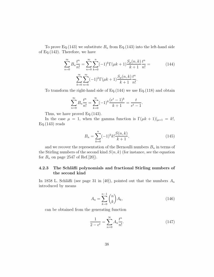
et − 1. (142)

These numbers play an important role in the number theory.Let’s show that the Bernoulli numbers Bn can be presented in terms of

the fractional Stirling numbers of the second kind Sµ(n, k) in the followingway

Bn =n∑

k=0

(−1)kΓ(µk + 1)Sµ(n, k)

k + 1. (143)

37

To prove Eq.(143) we substitute Bn from Eq.(143) into the left-hand sideof Eq.(142). Therefore, we have

∞∑

n=0

Bntn

n!=

∞∑

n=0

n∑

k=0

(−1)kΓ(µk + 1)Sµ(n, k)

k + 1

tn

n!= (144)

∞∑

k=0

∞∑

n=k

(−1)kΓ(µk + 1)Sµ(n, k)

k + 1

tn

n!.

To transform the right-hand side of Eq.(144) we use Eq.(118) and obtain

∞∑

n=0

Bntn

n!=

∞∑

k=0

(−1)k(et − 1)k

k + 1=

t

et − 1.

Thus, we have proved Eq.(143).In the case µ = 1, when the gamma function is Γ(µk + 1)|µ=1 = k!,

Eq.(143) reads

Bn =

n∑

k=0

(−1)kk!S(n, k)

k + 1, (145)

and we recover the representation of the Bernoulli numbers Bn in terms ofthe Stirling numbers of the second kind S(n, k) (for instance, see the equationfor Bn on page 2547 of Ref.[20]).

4.2.3 The Schlafli polynomials and fractional Stirling numbers of

the second kind

In 1858 L. Schlafli (see page 31 in [40]), pointed out that the numbers An

introduced by means

An =n−1∑

k=0

(

n

k

)

Ak, (146)

can be obtained from the generating function

1

2− et=

∞∑

n=0

Antn

n!. (147)

38

We will call the numbers An as the Schlafli numbers. The numbers An

can be expressed as

An =n∑

k=0

S(n, k)k!, (148)

where S(n, k) are the Stirling numbers of the second kind.Now we introduce the Schlafli polynomials An(x) defined by

An(x) =

n∑

k=0

S(n, k)k!xk. (149)

As an example, here are a few Schlafli polynomials

A0(x) = 1, A1(x) = x, A2(x) = 2x2 + x, ... .

Taking into account Eq.(113) we can express An(x) as

An(x) =

n∑

k=0

Sµ(n, k)Γ(µk + 1)xk, (150)

and

An =n∑

k=0

Sµ(n, k)Γ(µk + 1), (151)

where Sµ(n, k) are the fractional Stirling numbers of the second kind.Thus, we found the new representations of the Schlafli polynomials An(x)and the Schlafli numbers An in terms of the fractional Stirling numbers ofthe second kind.

The generating function A(t, x) of the Schlafli polynomials introduced by

A(t, x) =∞∑

n=0

tn

n!An(x), (152)

can be presented in terms of fractional Stirling numbers of the secondkind,

A(t, x) =∞∑

n=0

tn

n!

n∑

k=0

Sµ(n, k)Γ(µk + 1)xk, (153)

39

if we use the definition given by Eq.(150).Further, we have the following chain of transformations

A(t, x) =∞∑

n=0

tn

n!

(

n∑

k=0

Sµ(m, k)Γ(µk + 1)xk

)

=

∞∑

n=0

tn

n!

( ∞∑

k=0

θ(n− k)Sµ(n, k)Γ(µk + 1)xk

)

= (154)

∞∑

k=0

Γ(µk + 1)xk

( ∞∑

m=k

Sµ(m, k)tm

m!

)

, (155)

where θ(m− l) is the Heaviside step function defined by Eq.(105). Sub-stituting into Eq.(155) the internal sum over m with the right-hand side ofEq.(117) yields

A(t, x) =

∞∑

k=0

(et − 1)kxk =1

1− x(et − 1). (156)

Thus, we recover the generating function of the Schlafli polynomials (see,for instance, Eq.(9) in Ref.[41]). In the special case, when x = 1 Eq.(156)turns into Eq.(147).

At x = −1 it follows from Eqs.(153) and (156) that

n∑

k=0

Sµ(n, k)Γ(µk + 1)(−1)k = (−1)n. (157)

which is a new formula for the fractional Stirling numbers Sµ(n, k) of thesecond kind.

The Schlafli polynomials An(x) and fractional Bell polynomials Bµ(xλ, n),are related each other by

An(x) =

∞∫

0

dλLµ(λ)Bµ(xλ, n), (158)

where the kernel Lµ(λ) is

Lµ(λ) =λ(

1µ−1)

µexp

{

−λ1/µ}

. (159)

40

Equation (158) can be verified by using Eq.(102).

4.3 Fractional Stirling numbers of the first kind

To introduce fractional Stirling numbers of the first kind let us solve for xl

in Eq.(102),

1 = Bµ(x, 0),

x = Γ(µ+ 1)Bµ(x, 1),

x2 =Γ(2µ+ 1)

2!(Bµ(x, 2)− Bµ(x, 1)) , (160)

x3 =Γ(3µ+ 1)

3!(Bµ(x, 3)− 3Bµ(x, 2) + 2Bµ(x, 1)) ,

x4 =Γ(4µ+ 1)

4!(Bµ(x, 4)− 6Bµ(x, 3) + 11Bµ(x, 2)− 6Bµ(x, 1)) ,

and so forth. In general case we can write

xn =

n∑

k=0

sµ(n, k)Bµ(x, k), (161)

if we introduce a new numbers sµ(n, k) defined as

sµ(n, k) =Γ(nµ+ 1)

n!s(n, k), (162)

with s(n, k) being the Stirling numbers of the first kind [38]. We call newnumbers sµ(n, k) as fractional Stirling numbers of the first kind.

It follows from Eqs.(162) that

s(n, k) =n!

Γ(nµ+ 1)sµ(n, k). (163)

This equation allows us to find new equations and identities for the frac-tional Stirling numbers of the first kind sµ(n, k) based on the well-knowequations and identities for the standard Stirling numbers s(n, k) of the first

41

kind. For example, considering the recurrence relation for Stirling numbersof the first kind [38],

s(n + 1, k) = s(n, k − 1)− ns(n, k), 1 ≤ k ≤ n,

yields the recurrence relation for the fractional Stirling numbers of thefirst kind

(n+ 1)Γ(nµ+ 1)

Γ((n+ 1)µ+ 1)sµ(n+ 1, k) = sµ(n, k − 1)− nsµ(n, k), 1 ≤ k ≤ n.

(164)It is easy to check that

n∑

k=0

sµ(n, k) = 0, n > 1, (165)

and

n∑

k=1

(−1)n−ksµ(n, k) = Γ(nµ+ 1). (166)

Some special cases are

sµ(n, 0) = δn,0, sµ(n, 1) =(−1)n−1

nΓ(nµ+ 1), (167)

and

sµ(n, n− 1) = −Γ(nµ+ 1)

2(n− 2)!, sµ(n, n) =

Γ(nµ+ 1)

n!. (168)

As an example, Table 6 presents a few fractional Stirling numbers of thefirst kind.

n\k 1 2 3 4 5 61 Γ(µ+ 1)

2 -Γ(2µ+1)2

Γ(2µ+1)2

3 Γ(3µ+1)3

-Γ(3µ+1)2

Γ(3µ+1)6

4 -Γ(4µ+1)4

-11Γ(4µ+1)24

-Γ(4µ+1)4

Γ(4µ+1)24

5 Γ(5µ+1)5

-5Γ(5µ+1)12

7Γ(5µ+1)24

-Γ(5µ+1)12

Γ(5µ+1)120

6 -Γ(6µ+1)6

137Γ(6µ+1)360

-5Γ(6µ+1)16

17Γ(6µ+1)144

-Γ(6µ+1)48

Γ(6µ+1)720

Table 6. Fractional Stirling numbers of the first kind sµ(n, k) (0 < µ ≤ 1).

42

5 Statistics of the fractional Poisson proba-

bility distribution

5.1 Moments of the fractional Poisson probability dis-

tribution

Now we use the fractional Stirling numbers of the second kind introducedby Eq.(107) to get the moments and the central moments of the fractionalPoisson probability distribution given by Eq.(9). Indeed, by definition of them-th order moment of the fractional Poisson probability distribution we have

nmµ =

∞∑

n=0

nmPµ(n, t) =∞∑

n=0

nm (νtµ)n

n!

∞∑

k=0

(k + n)!

k!

(−νtµ)kΓ(µ(k + n) + 1)

, 0 < µ ≤ 1.

(169)It is easy to see that nm

µ is in fact the fractional Bell polynomial Bµ(νtµ, m)

introduced by Eq.(41),

nmµ = Bµ(νt

µ, m), m = 0, 1, 2, ..., 0 < µ ≤ 1. (170)

From other side, with the help of Eqs.(41) and (102) we find

nmµ =

m∑

l=0

Sµ(m, l)(νtµ)l. (171)

Hence, the fractional Stirling numbers Sµ(m, l) of the second kind natu-rally appear in the power series over νtµ for the m-th order moment of thefractional Poisson probability distribution.

Using analytical expressions given by Eqs.(107) and (171), let’s list a fewmoments of the fractional Poisson probability distribution

nµ =∞∑

n=0

nPµ(n, t) =νtµ

Γ(µ+ 1)= Bµ(νt

µ, 1), (172)

n2µ =

∞∑

n=0

n2Pµ(n, t) =2(νtµ)2

Γ(2µ+ 1)+

νtµ

Γ(µ+ 1)= Bµ(νt

µ, 2), (173)

43

n3µ =

∞∑

n=0

n3Pµ(n, t) =6(νtµ)3

Γ(3µ+ 1)+

6(νtµ)2

Γ(2µ+ 1)+

νtµ

Γ(µ+ 1)= Bµ(νt

µ, 3),

(174)

n4µ =

∞∑

n=0

n4Pµ(n, t) = (175)

24(νtµ)4

Γ(4µ+ 1)+

36(νtµ)3

Γ(3µ+ 1)+

14(νtµ)2

Γ(2µ+ 1)+

νtµ

Γ(µ+ 1)= Bµ(νt

µ, 4), (176)

here Bµ(νtµ, n), n = 1, 2, 3, 4, are fractional Bell polynomials introduced

by Eqs.(41).In terms of the power series over the first order moment nµ, the above

equations (173) - (175) read

n2µ =

2(Γ(µ+ 1))2

Γ(2µ+ 1)n2µ + nµ, (177)

n3µ =

6(Γ(µ+ 1))3

Γ(3µ+ 1)n3µ +

6(Γ(µ+ 1))2

Γ(2µ+ 1)n2µ + nµ, (178)

n4µ =

24(Γ(µ+ 1))4

Γ(4µ+ 1)n4µ +

36(Γ(µ+ 1))3

Γ(3µ+ 1)n3µ +

14(Γ(µ+ 1))2

Γ(2µ+ 1)n2µ + nµ. (179)

For the first time the mean nµ Eq.(172) and the second order moment n2µ

were obtained by Laskin6 (see, Eqs.(26) and (27) in Ref.[9]).In the case when µ = 1, equations (177) - (179) become the well-know

equations for moments of the standard Poisson probability distribution withthe parameter n ≡ n1 = νt (for instance, see Eqs.(22) - (24) in Ref. [42]).

6The second order moment defined by Eq.(177) can be presented as Eq.(27) of Ref.[9]

n2µ =

∞∑

n=0

n2Pµ(n, t) = nµ + n2

µ

√πΓ(µ+ 1)

22µ−1Γ(µ+ 1

2).

if we take into account the well-know equations for the gamma function Γ(µ)

Γ(µ+ 1) = µΓ(µ), Γ(2µ) =22µ−1

√π

Γ(µ) · Γ(µ+1

2).

44

5.2 Variance, skewness and kurtosis of the fractional

Poisson probability distribution

To find analytical expressions for variance, skewness and kurtosis of the frac-tional Poisson probability distribution, let’s introduce the central m-th ordermoment Mµ(m)

Mµ(m) = (nµ − nµ)m =

∞∑

n=0

(n− nµ)mPµ(n, t) =

∞∑

n=0

m∑

r=0

(−1)m−r

(

m

r

)

nr(nµ)m−rPµ(n, t) = (180)

m∑

r=0

(−1)m−r

(

m

r

)

(nµ)m−r

r∑

l=0

Sµ(r, l)(νtµ)l,

where Sµ(r, l) is given by Eq.(107).Hence, in terms of power series over the first order moment nµ given by

Eq.(172), we have

Mµ(1) = 0, (181)

Mµ(2) =

(

2(Γ(µ+ 1))2

Γ(2µ+ 1)− 1

)

n2µ + nµ, (182)

Mµ(3) = 2

(

3(Γ(µ+ 1))3

Γ(3µ+ 1)− 3(Γ(µ+ 1))2

Γ(2µ+ 1)+ 1

)

n3µ+ (183)

3

(

2(Γ(µ+ 1))2

Γ(2µ+ 1)− 1

)

n2µ + nµ,

Mµ(4) = 3

(

8(Γ(µ+ 1))4

Γ(4µ+ 1)− 8(Γ(µ+ 1))3

Γ(3µ+ 1)+

4(Γ(µ+ 1))2

Γ(2µ+ 1)− 1

)

n4µ+ (184)

6

(

6(Γ(µ+ 1))3

Γ(3µ+ 1)− 4(Γ(µ+ 1))2

Γ(2µ+ 1)+ 1

)

n3µ + 2

(

7(Γ(µ+ 1))2

Γ(2µ+ 1)− 2

)

n2µ + nµ.

45

Further, in terms of the above defined central moments Mµ(m), the vari-ance σ2, skewness sµ, and kurtosis kµ of the fractional Poisson probabilitydistribution are

σ2µ =Mµ(2), (185)

sµ =Mµ(3)

M3/2µ (2)

, (186)

kµ =Mµ(4)

M2µ(2)

− 3. (187)

In the case when µ = 1, new equations (182) - (184) turn into equationsfor the central moments of the standard Poisson probability distribution withthe parameter n ≡ n1 = νt (see, Eqs.(25) - (27) in Ref. [42]).

Equations (185) - (187), at µ = 1, turn into the equations for variance,skewness, and kurtosis of the standard Poisson probability distribution withthe parameter n ≡ n1 = νt (for instance, see Eqs.(29) - (31) in Ref. [42]).

6 New polynomials

6.1 Generating functions

6.1.1 Multiplicative renormalization framework

It is well known from the theory of orthogonal polynomials [27] that orthog-onal polynomials of discrete variable are associated with discrete probabilitydistributions. Fractional Poisson probability distribution is a new member ofthe family of discrete probability distributions. Thus, based on our findingswe now post the challenge to design and develop a new system of polynomialsassociated with fractional Poisson probability distribution

Pµ(x, λµ) =(λµ)

x

x!

∞∑

k=0

(k + x)!

k!

(−λµ)kΓ(µ(k + x) + 1)

, 0 < µ ≤ 1, (188)

where x is discrete random variable (x = 0, 1, 2, ...) and λµ is parameter.To meet the challenge we will follow the idea of a multiplicative renor-

malization framework [23]. Thus, let’s consider the function

46

ϕ(t, x) = (1 + t)x, (189)

where we treat x as a discrete random variable with fractional Poissonprobability distribution, see, Eq.(188). Then, the multiplicative renormal-ization ψµ(t, x) is defined by

ψµ(t, x) =ϕ(t, x)

< ϕ(t, x) >Pµ

, (190)

here <...>Pµstands for expectation over Pµ(x, λ) given by Eq.(188), that

is

< ϕ(t, x) >Pµ=

∞∑

x=0

Pµ(x, λµ)ϕ(t, x). (191)

Then, evaluating the expectation <...>Pµyields

ψµ(t, x) =ϕ(t, x)

Eµ(λµt), (192)

where Eµ(λt) is the Mittag-Leffler function defined by Eq.(8).Function ψµ(t, x) is the multiplicative renormalization of function ϕ(t, x)

in Eq.(189) over the probabilistic measure associated with fractional Poissonprobability distribution Eq.(188).

Multiplicative renormalization framework [23] says that the multiplicativerenormalization ψ(t, x) can be considered as a generating function of newpolynomials Ln(x;λµ). That is

ψµ(t, x) =(1 + t)x

Eµ(λt)=

∞∑

n=0

Ln(x;λµ)tn

n!, 0 < µ ≤ 1, (193)

where n-degree polynomials Ln(x;λµ) of discrete variable x depend onthe value of real parameter λ and parameter µ associated with fractionalPoisson probability distribution.

At x = 0 Eq.(193) can be considered as the definition for generatingfunction φµ(t) = ψµ(t, 0) of new numbers Ln(λµ) = Ln(0;λµ)

φµ(t) =1

Eµ(λµt)=

∞∑

n=0

Ln(λµ)tn

n!, 0 < µ ≤ 1, (194)

47

To obtain explicit expressions for polynomials Ln(x;λµ) we write

1

Eµ(λµt)=

∞∑

k=0

ak(µ)(λµt)

k

k!, (195)

with yet unknown coefficients ak(µ) that have to be found.With help of Eq.(195) the generating function ψµ(t, x) reads

ψµ(t, x) =∞∑

n=0

(

x

n

)

tn∞∑

k=0

ak(µ)(λµt)

k

k!=

∞∑

n=0

tn

n!

(

n∑

k=0

n!

(n− k)!λn−kµ

(

x

k

)

an−k(µ)

)

,

(196)where notation

(

xn

)

= x!n!(x−n)!

has been used.

Comparing Eqs.(193) and (196) gives us an explicit formula for new poly-nomials Ln(x;λµ),

Ln(x;λµ) =n∑

k=0

n!

(n− k)!λn−kµ

(

x

k

)

an−k(µ), (197)

while comparing Eqs.(194) and (196) gives us explicit formula for newnumbers Ln(λµ)

Ln(λµ) = λnµan(µ). (198)

Polynomials Ln(x;λµ) can be written as

Ln(x;λµ) =

n∑

k=0

(

n

k

)

λn−kµ an−k(µ)

k∑

l=0

s(k, l)xl, (199)

or

Ln(x;λµ) =

n∑

l=0

xln∑

k=l

(

n

k

)

λn−kµ an−k(µ)s(k, l), (200)

where s(k, l) are the Stirling numbers of the first kind [38].Aiming to find coefficients an(µ) we rewrite Eq.(195) as

∞∑

m=0

(λµt)m

Γ(µm+ 1)

∞∑

k=0

ak(µ)(λµt)

k

k!= 1. (201)

48

Then, the Cauchy product rule yields for the left hand side of Eq.(201)

∞∑

m=0

(λµt)m

Γ(µm+ 1)

∞∑

k=0

ak(µ)(λµt)

k

k!=

∞∑

n=0

cn(µ)(λµt)

n

n!, (202)

where

cn(µ) =n∑

l=0

n!

(n− l)!

an−k(µ)

Γ(µl + 1). (203)

From Eqs.(201)-(203) we come to the conclusion that

c0(µ) = 1, cn(µ) = 0, n ≥ 1. (204)

Hence, we have

a0(µ) = c0(µ) = 1, (205)

and

n∑

l=0

n!

(n− l)!

an−l(µ)

Γ(µl + 1)= 0, n ≥ 1. (206)

The last equation results in

an(µ) = −n∑

l=1

n!

(n− l)!

an−l(µ)

Γ(µl + 1), n ≥ 1. (207)

The system of two equations (207) and (205) can be iterated to obtainan(µ). As an example, here are explicit expressions for a few coefficients an(µ)

a1(µ) = − 1

Γ(µ + 1), (208)

a2(µ) =2

(Γ(µ+ 1))2− 2

Γ(2µ+ 1), (209)

a3(µ) = − 6

(Γ(µ+ 1))3+

12

Γ(µ+ 1)Γ(2µ+ 1)− 6

Γ(3µ+ 1). (210)

Now we can present a few new polynomials Ln(x;λµ), 0 < µ ≤ 1

49

L0(x;λµ) = 1, (211)

L1(x;λµ) = x− λµΓ(µ+ 1)

, (212)

L2(x;λµ) = x2−x(1+2λµ

Γ(µ+ 1))+2λ2µ

(

1

(Γ(µ+ 1))2− 1

Γ(2µ+ 1)

)

. (213)

L3(x;λµ) = x3 − 3x2(

1 +λµ

Γ(µ+ 1)

)

+ x

(

2 + 6λ2µ

(

1

(Γ(µ+ 1))2− 1

Γ(2µ+ 1)

)

+3λµ

Γ(µ+ 1)

)

(214)

+ 6λ3µ

(

− 1

(Γ(µ+ 1))2+

2

Γ(µ+ 1)Γ(2µ+ 1)− 1

Γ(3µ+ 1)

)

, (215)

and a few new numbers Ln(λµ)

L0(λµ) = 1, (216)

L1(λµ) = − λµΓ(µ + 1)

, (217)

L2(λµ) = 2λ2µ

(

1

(Γ(µ+ 1))2− 1

Γ(2µ+ 1)

)

. (218)

L3(λµ) = 6λ3µ

(

− 1

(Γ(µ+ 1))2+

2

Γ(µ+ 1)Γ(2µ+ 1)− 1

Γ(3µ+ 1)

)

. (219)

Newly introduced polynomials Ln(x;λµ) do not form a system of orthog-onal polynomials, because of non-Markov property of the fractional Poissonprobability distribution. To illustrate this statement let’s follow the multi-plicative renormalization framework [23] and calculate< ψµ(s, x)ψµ(t, x) >Pµ

,

50

< ψµ(s, x)ψµ(t, x) >Pµ=

∞∑

x=0

Pµ(x, λµ)(1 + s)x

Eµ(λµs)

(1 + t)x

Eµ(λµt)= (220)

Eµ(λµs + λµt+ λµst)

Eµ(λµs)Eµ(λµt),

where Pµ(x, λµ) is given by Eq.(188).The multiplicative renormalization framework [23] says that if, and only

if, the expectation of the product of two generating functions< ψ(t, x)ψ(s, x) >Pµ

is function of st, then it implies orthogonality of the polynomials generatedby ψµ(t, x). It is not the case for the generating function Eq.(193), becauseof the presence of the Mittag-Leffler functions in the right side of Eq.(220).

In the limit case µ = 1 the probability distribution function Pµ(x, λµ)|µ=1

defined by Eq.(188) becomes the well-known Poisson probability distributionP (x, λ) with λ = λµ|µ=1,

P (x, λ) =(λ)x

x!e−λ, (221)

which posses the Markov property. Further, the generating functionψ(t, x) = ψµ(t, x)|µ=1 becomes

ψ(t, x) =ϕ(t, x)

eλt, (222)

with ϕ(t, x) given by Eq.(189). Thus, we obtain,

ψ(t, x) = (1 + t)xe−λt =

∞∑

n=0

tn

n!Cn(x;λ), (223)

which is recognizable as the generating function of the Charlier orthogonalpolynomials Cn(x;λ) of discrete variable x [27] associated with the Poissonprobability distribution.

It is easy to see, that

< ψ(s, x)ψ(t, x) >P=∞∑

x=0

P (x, λ)(1 + s)xe−λs(1 + t)xe−λt = eλst, (224)

51

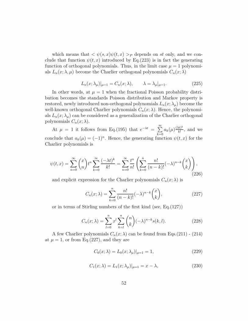
which means that < ψ(s, x)ψ(t, x) >P depends on st only, and we con-clude that function ψ(t, x) introduced by Eq.(223) is in fact the generatingfunction of orthogonal polynomials. Thus, in the limit case µ = 1 polynomi-als Ln(x;λ, µ) become the Charlier orthogonal polynomials Cn(x;λ)

Ln(x;λµ)|µ=1 = Cn(x;λ), λ = λµ|µ=1. (225)

In other words, at µ = 1 when the fractional Poisson probability distri-bution becomes the standards Poisson distribution and Markov property isrestored, newly introduced non-orthogonal polynomials Ln(x;λµ) become thewell-known orthogonal Charlier polynomials Cn(x;λ). Hence, the polynomi-als Ln(x;λµ) can be considered as a generalization of the Charlier orthogonalpolynomials Cn(x;λ).

At µ = 1 it follows from Eq.(195) that e−λt =∞∑

k=0

ak(µ)(λt)k

k!, and we

conclude that ak(µ) = (−1)n. Hence, the generating function ψ(t, x) for theCharlier polynomials is

ψ(t, x) =∞∑

n=0

(

x

n

)

tn∞∑

k=0

(−λt)kk!

=∞∑

n=0

tn

n!

(

n∑

k=0

n!

(n− k)!(−λ)n−k

(

x

k

)

)

,

(226)and explicit expression for the Charlier polynomials Cn(x;λ) is

Cn(x;λ) =

n∑

k=0

n!

(n− k)!(−λ)n−k

(

x

k

)

, (227)

or in terms of Stirling numbers of the first kind (see, Eq.(127))

Cn(x;λ) =n∑

l=0

xln∑

k=l

(

n

k

)

(−λ)n−ks(k, l). (228)

A few Charlier polynomials Cn(x;λ) can be found from Eqs.(211) - (214)at µ = 1, or from Eq.(227), and they are

C0(x;λ) = L0(x;λµ)|µ=1 = 1, (229)

C1(x;λ) = L1(x;λµ)|µ=1 = x− λ, (230)

52

C2(x;λ) = L2(x;λµ)|µ=1 = x2 − x(1 + 2λ) + λ2, (231)

C3(x;λ) = L3(x;λµ)|µ=1 = x3 − 3x2(1 + λ) + x(

2 + 3λ+ 3λ2)

− λ3, (232)

where λ = λµ|µ=1.From Eqs.(223) and (226) we have

∞∑

x=0

(λ)x

x!e−λ

∞∑

n=0

sn

n!Cn(x;λ)

∞∑

m=0

tm

m!Cm(x;λ) =

∞∑

n=0

λn(st)n

n!. (233)

Thus, we obtain

∞∑

n=0

∞∑

m=0

( ∞∑

x=0

(λ)x

x!e−λCn(x;λ)Cm(x;λ)

)

sn

n!

tm

m!=

∞∑

n=0

λn(st)n

n!. (234)

Comparison of the coefficients in Eq.(234) leads to the orthogonality con-dition for the Charlier polynomials

∞∑

x=0

(λ)x

x!e−λCn(x;λ)Cm(x;λ) = λnn!δn,m, (235)

where δn,m is the Kronecker symbol.Table 7 compares equations for newly introduced polynomials Ln(x;λµ)

vs the Charlier orthogonal polynomials Cn(x;λ). Table 7 presents two setsof equations for probability distribution function P (x, λ) of discrete randomvariable x, polynomials generating function ψ(t, x), generating function φ(t)of numbers, expectation of the product of two multiplicative renormalizationfunctions < ψ(t, x)ψ(s, x) > and orthogonality condition.

53

Polynomials Ln(x;λµ) (0 < µ ≤ 1) Charlier polynomials Cn(x;λ) (µ = 1)

P (x, λ) (λµ)x

x!

∞∑

k=0

(k+n)!k!

(−λµ)k

Γ(µ(k+n)+1)(λ)x

x!exp(−λ)

ψ(t, x) (1+t)x

Eµ(λµt)=

∞∑

n=0

Ln(x;λµ)tn

n!(1 + t)xe−λt =

∞∑

n=0

tn

n!Cn(x;λ)

φ(t) 1Eµ(λµt)

=∞∑

n=0

Ln(λµ)tn

n!e−λt =

∞∑

n=0

tn

n!Cn(λ)

< ψ(s, x)ψ(t, x) > Eµ(λµs+λµt+λµst)Eµ(λµs)Eµ(λµt)

eλst

Orthogonality Non-orthogonal∞∑

x=0

(λ)xe−λ

x!Cn(x;λ)Cm(x;λ) = λnn!δn,m

Table 7. Multiplicative renormalization formulas related to the polynomi-

als Ln(x;λµ) vs the Charlier polynomials Cn(x;λ).

6.1.2 Alternative approach

As an alternative to the multiplicative renormalization framework, we de-velop an approach to build polynomial sequence ln(x;λµ) based on generatingfunction gµ(t, x) introduced by,

gµ(t, x) = (1 + t)xEµ(−λµt) =

∞∑

n=0

ln(x;λµ)tn

n!, 0 < µ ≤ 1, (236)

where Eµ(x) is the Mittag-Leffler function (see, definition given by Eq.(8)).The n-degree polynomials ln(x;λµ) of discrete variable x depend on the valueof real parameter λµ and parameter µ associated with fractional Poisson prob-ability distribution given by Eq.(188). The motivation behind Eq.(236) is anattempt to get polynomial sequence ln(x;λµ) which coincides with the Char-lier orthogonal polynomials at µ = 1 and is alternative to the polynomialsequence Ln(x;λµ) introduced by Eq.(193).

At x = 0 Eq.(236) can be considered as the definition for generatingfunction jµ(t) = gµ(t, 0) of numbers ln(λµ) = ln(0;λµ)

jµ(t) = Eµ(−λµt) =

∞∑

n=0

ln(λµ)tn

n!, 0 < µ ≤ 1. (237)

It follows from Eq.(236) that

54

gµ(t, x) =∞∑

n=0

(

x

n

)

tn∞∑

k=0

(−λµt)k

Γ(µk + 1)= (238)

∞∑

n=0

tn

n!

(

n∑

k=0

n!

Γ(µ(n− k) + 1)(−λµ)n−k

(

x

k

)

)

. (239)

Thus, we have

ln(x;λµ) =

n∑

k=0

n!

Γ(µ(n− k) + 1)(−λµ)n−k

(

x

k

)

, (240)

or

ln(x;λµ) =

n∑

l=0

xln∑

k=l

n!

k!Γ(µ(n− k) + 1)(−λµ)n−ks(k, l), 0 < µ ≤ 1,

(241)where s(k, l) are Stirling numbers of the first kind [38].A few new polynomials ln(x;λµ), 0 < µ ≤ 1 are

l0(x;λµ) = 1, (242)

l1(x;λµ) = x− λµΓ(µ+ 1)

, (243)

l2(x;λµ) = x2 − x(1 +2λµ

Γ(µ+ 1)) +

2λ2µΓ(2µ+ 1)

, (244)

l3(x;λµ) = x3−3x2(1+λµ

Γ(µ+ 1))+x

(

2 +3λµ

Γ(µ+ 1)+

6λ2µΓ(2µ+ 1)

)

−6λ3µ

Γ(3µ+ 1).

(245)The numbers ln(λµ), 0 < µ ≤ 1 are given by

ln(λµ) = (−λµ)n n!

Γ(nµ+ 1). (246)

Newly introduced polynomials ln(x;λµ) do not form a system of orthog-onal polynomials. In the limit case µ = 1 Eq.(236) goes into Eq.(223) and

55

we come to the generating function of the Charlier orthogonal polynomi-als. Hence, at µ = 1 newly introduced polynomials ln(x;λµ)|µ=1 become theCharlier orthogonal polynomials, ln(x;λµ)|µ=1 = Cn(x;λ).

7 Conclusions

Applications of the fractional Poisson probability distribution to quantumphysics, number theory and theory of polynomials have been presented.

As a quantum physics application, a new family of quantum coherentstates has been introduced and explored to study physical phenomena wherethe distribution of photon numbers is governed by the fractional Poissonprobability distribution.

As number theory applications we have discovered and developed the frac-tional generalization of Bell polynomials, Bell numbers, and Stirling numbersof the first kind and the second kind. Appearance of fractional Bell polyno-mials is natural if one evaluates the diagonal matrix element of the evolutionoperator in the basis of newly introduced quantum coherent states. Frac-tional Stirling numbers of the second kind have been introduced and appliedto evaluate skewness and kurtosis of the fractional Poisson probability distri-bution function. A new representation of the Bernoulli numbers in terms offractional Stirling numbers of the second kind has been obtained. A represen-tation of Schlafli polynomials in terms of fractional Stirling numbers of thesecond kind has been found. The integral relationship between the Schlaflipolynomials and fractional Bell polynomials has been obtained. A new rep-resentation of the Mittag-Leffler function involving fractional Bell polynomi-als and fractional Stirling numbers of the second kind has been discovered.Fractional Stirling numbers of the first kind have also been introduced andstudied.

Two new sequences of polynomials of discrete variable associated withfractional Poisson probability distribution has been launched and explored.The relationship between new polynomials and the orthogonal Charlier poly-nomials has also been investigated.

In the limit case when the fractional Poisson probability distribution be-comes the Poisson probability distribution, all of the above listed develop-ments and implementations turn into the well-known results of the quantumoptics, the theory of combinatorial numbers and the theory of orthogonalpolynomials of discrete variable.

56

Table 1 compares fundamental equations associated with the fractionalPoisson probability distribution to those of the well-known ones, related tothe standard Poisson probability distribution. Tables 2, 3, 4, 5, 6 and 7summarize our findings for the fractional Poisson probability distributionin comparison to the well-known results attributed to the standard Poissonprobability distribution.

These findings facilitate the further exploration of long-memory impacton quantum phenomena and initiate studies on fundamental relationshipsbetween orthogonality of polynomials and the Markov property of underlyingprobabilistic distributions involved into multiplicative renormalization.

8 Appendix

To obtain Eq.(28) we use the Laplace transform of the Mittag-Leffler functionEµ(−zτµ)

∞∫

0

dτe−τEµ(−zτµ) =1

1 + z,

for instance, see equation (26) on page 210 of Ref.[32].Changing the variable τ → st and the parameter zsµ → ζ yields

∞∫

0

dte−stEµ(−ζtµ) =sµ−1

sµ + ζ. (247)

By differentiating Eq.(247) n times with respect to ζ we obtain,

∞∫

0

dte−sttµnE(n)µ (−ζtµ) = n! · sµ−1

(sµ + ζ)n+1. (248)

It is easy to see that at ζ = µ Eq.(248) goes into Eq.(28).

References

[1] N. Laskin, Fractional quantum mechanics and Levy path integrals, Phys.Lett. A268 (2000) 298-305.

57

[2] N. Laskin, Fractional quantum mechanics, Phys.Rev. E62 (2000) 3135–3145 (also available online:http://arxiv.org/PS cache/arxiv/pdf/0811/0811.1769v1.pdf).

[3] N. Laskin, Fractals and quantum mechanics, Chaos 10 (2000) 780-790.

[4] N. Laskin, Fractional Schrodinger equation, Phys.Rev. E66 (2000) 3135–3145 (also available online:http://arxiv.org/PS cache/quant-ph/pdf/0206/0206098v1.pdf).

[5] N. Laskin, Levy flights over quantum paths, Communications in Non-linear Science and Numerical Simulation 12 (2007) 2-18 (also availableonline: http://arxiv.org/PS cache/quant-ph/pdf/0504/0504106v1.pdf).

[6] N. Laskin, Principles of Fractional Quantum mechanics, in J. Klafter,S.C Lim, R. Metzler (Eds.), Fractional Dynamics, Recent Advances(World Scientific, Singapore, 2011), pp.393-427.

[7] R.P. Feynman, The Space-Time Formulation of Nonrelativistic Quan-tum Mechanics, Rev. Mod. Phys. 20 (1948) 367–387.

[8] R. P. Feynman and A.R. Hibbs, QuantumMechanics and Path Integrals,McGraw-Hill, New York, 1965.

[9] N. Laskin, Fractional Poisson process, Communications in NonlinearScience and Numerical Simulation, 8 (2003) 201-213.

[10] M. Kuno, D.P. Fromm, H. F. Hamann, A. Gallagher, and D.J. Nes-bitt, Nonexponential blinking kinetics of single CdSe quantum dots: Auniversal power law behavior, J. Chem. Phys. 112 (2000) 3117-3120.

[11] L. Sabatelli et al, Waiting time distributions in financial markets, TheEuropean Physical Journal B - Condensed Matter and Complex Sys-tems, 27 (2002) 273-275.

[12] W. Willinger, and V. Paxson, Where Mathematics Meets the Internet,Notices of the American Mathematical Society, 45 (1998) 961-970.

[13] A. I. Saichev and G.M. Zaslavsky, Fractional kinetic equations: solutionsand applications, Chaos 7 (1997) 753-764.

58

http://arxiv.org/PS_cache/arxiv/pdf/0811/0811.1769v1.pdf

http://arxiv.org/PS_cache/quant-ph/pdf/0206/0206098v1.pdf

http://arxiv.org/PS_cache/quant-ph/pdf/0504/0504106v1.pdf

[14] N. Laskin, Some applications of the fractional Poisson probability dis-tribution, J Math Phys 50 (2009) 113513.

[15] N. Laskin, New Polynomials and Numbers Associated withFractional Poisson Probability Distribution, ICNAAM 2010:International Conference of Numerical Analysis and Ap-plied Mathematics 2010, Rhodes (Greece), AIP ConferenceProceedings 1281, (2010) 1152-1155. (also available online:http://arxiv.org/PS cache/arxiv/pdf/1010/1010.2874v1.pdf).

[16] J.R. Klauder, The Current State of Coherent States,arXiv:quant-ph/0110108v1 17 Oct 2001.

[17] E. T. Bell, Exponential Polynomials, The Annals of Mathematics, Sec-ond Series, 35 (1934), 258-277.

[18] J. Stirling, Methodus Differentialis: Sive Tractatus de Summatione etInterpolatione Serierum Infinitarum, Gul. Bowyer, London, 1730. (En-glish translation by I. Tweddle, James Stirling’s Methodus Differentialis:An Annotated Translation of Stirling’s Text Springer, London, 2003).

[19] C. A. Charalambides, Enumerative combinatorics, Ch.8, Chap-man&Hall/CRC, 2002.

[20] C. A. Charalambides and J. Singh: A review of the Stirling numbers,their generalizations and statistical applications, Communications inStatistics - Theory and Methods, 17 (1988) 2533-2595.

[21] G. Dobinski, Summirung der Reihe∑

nm/n!, fur m = 1, 2, 3, 4, 5, ...,Grunert Archiv Arch. fur M. und Physik 61 (1877) 333-336.

[22] Gian-Carlo Rota, The Number of Partitions of a Set, American Mathe-matical Monthly, 71 (1964) 498–504.

[23] N. Asai, I. Kubo and H. Kuo, Multiplicative renormalization and gener-ating functions I, Taiwaneese Journal of Mathematics, 7 (2003) 89-101.

[24] J.R. Klauder, E.C.G. Sudarshan, Fundamentals of Quantum Optics,Benjamin, New York, 1968.

[25] R. J. Glauber, Quantum Theory of Optical Coherence. Selected Papersand Lectures, Wiley-VCH, Weinheim 2007.

59

http://arxiv.org/PS_cache/arxiv/pdf/1010/1010.2874v1.pdf

http://arxiv.org/abs/quant-ph/0110108

[26] L. Mandel and E. Wolf, Optical Coherence and Quantum Optics, Cam-bridge University Press, 1995.

[27] T. S. Chihara, An Introduction to Orthogonal Polynomials (Mathemat-ics and Its Applications), Gordon and Breach, Science Publishers, NewYork, NY, 1978.

[28] K.B. Oldham and J. Spanier, The Fractional Calculus, Academic Press,New York, 1974.

[29] S.G. Samko, A.A. Kilbas, and O.I. Marichev, Fractional Integrals andDerivatives and Their Applications, Gordon and Breach Science Pub-lishers, Langhorne, PA, 1993.

[30] K.S. Miller and B. Ross, An Introduction to the Fractional Calculus andFractional Differential Equations, J. Wiley & Sons, New York, 1993.

[31] G. Mittag-Leffler, Sur la repriesentation analytique d’une branche uni-forme d’une fonction monogene, Acta Mathematics, 29 (1905) 101-182.

[32] A. Erdelyi, Ed., Higher Transcendental Functions, Vol.3, pp. 206-227(Chapter 18 Miscellaneous Functions) McGraw-Hill, New York, 1955.

[33] E. Schrodinger, Der stetige Ubergang von der Mikro-zurMakromechanik, Die Naturwissenschaften 14 (1926) 664-666.

[34] J.-M. Sixdeniers, K. A. Penson, and A. I. Solomon, J. Phys. A32 (1999)7543-7564.

[35] J. Katriel, Bell numbers and coherent states, Phys. Lett. A 273 (2000)159-161.

[36] Abramowitz, M. and Stegun, I. A. (Eds.). ”Beta Function” §6.2 in Hand-book of Mathematical Functions with Formulas, Graphs, and Mathe-matical Tables, 9th printing, p. 258, New York, Dover, 1972.

[37] M. Abramowitz and I.A. Stegun, (Eds.). Stirling Numbers of the SecondKind. §24.1.4 in Handbook of Mathematical Functions with Formulas,Graphs, and Mathematical Tables, 9th printing, pp. 824-825, New York,Dover, 1972.

60

[38] M. Abramowitz and I.A. Stegun, (Eds.). Stirling Numbers of the FirstKind. §24.1.3 in Handbook of Mathematical Functions with Formulas,Graphs, and Mathematical Tables, 9th printing, p. 824, New York,Dover, 1972.

[39] M. Abramowitz and I.A. Stegun, (Eds.). Bernoulli and Euler Polynomi-als and the Euler-Maclarin Formula §23.1 in Handbook of MathematicalFunctions with Formulas, Graphs, and Mathematical Tables, 9th print-ing, pp. 804, New York, Dover, 1972.

[40] L. Schlafli “On a generalization given by Laplace of Lagrange’s Theo-rem”, Quarterly Journal of Pure and Applied Mathematics, 2 (1858)24-31.

[41] S.M. Tanny, On some numbers related to the Bell numbers, Canad.Math. Bull. 17 (1975), 733-738.

[42] E.W. Weisstein, Poisson Distribution, From MathWorld - A WolframWeb Resource,

http://mathworld.wolfram.com/PoissonDistribution.html.

61

http://mathworld.wolfram.com/PoissonDistribution.html

Some applications of the fractional Poisson probability distribution

Documents

Transcript of Some applications of the fractional Poisson probability distribution