Itinerant Oscillator Models of Fluids

ITINERANT OSCILLATOR MODELS OF FLUIDS

WILLIAM T. COFFEY

Department of Electronic and Electrical Engineering, School of Engineering,

Trinity College, Dublin, Ireland

YURI P. KALMYKOV

Centre d’Etudes Fondamentales, Universite de Perpignan, Perpignan, France

SERGEY V. TITOV

Institute of Radio Engineering and Electronics of the Russian Academy of

Sciences, Fryazino, Moscow Region, Russian Federation

CONTENTS

I. Introduction

II. Application of the Itinerant Oscillator (Cage) Model to the Calculation of the

Dielectric Absorption Spectra of Polar Molecules

A. Generalization of the Onsager Model—Relation to the Cage Model

B. Calculation of the Dipole Correlation Function

C. Exact Solution for the Complex Susceptibility Using Matrix Continued Fractions

D. Approximate Expressions for the Complex Susceptibility

E. Numerical Results and Comparison with Experimental Data

F. Conclusions

III. Application to Ferrofluids

A. Langevin Equation Formalism

B. Precession-Aided Effects in Neel Relaxation

C. Effect of the Fluid Carrier: (i) Response to a Weak Applied Field

D. Effect of the Fluid Carrier: (ii) Mode–Mode Coupling Effects for Particles with

Uniaxial Anisotropy in a Strong Applied Field

E. Comparison with Experimental Observations of the Complex Susceptibility Data

F. Conclusions

131

Advances in Chemical Physics, Volume 126Edited by I. Prigogine and Stuart A. Rice

Copyr ight 2003 John Wiley & Sons, I nc.ISBN: 0-471-23582-2

IV. Anomalous Diffusion

A. Application of Continuous-Time Random Walks in Rotational Relaxation

B. The Fractional Klein–Kramers Equation

C. Solution of the Fractional Klein–Kramers Equation

D. Dielectric Loss Spectra

E. Angular Velocity Correlation Function

F. Conclusions

Acknowledgments

References

I. INTRODUCTION

The itinerant oscillator introduced by Hill [1] and Sears [2] is a model for the

dynamical (rotational or translational) behavior of a molecule in a fluid

embodying the suggestion that a typical molecule of the fluid is capable of

vibration in a temporary equilibrium position (cage), which itself undergoes

Brownian motion. Sears [2] used a translational version of the model (see Fig. 1)

to evaluate the velocity correlation function for liquid argon, while a two-

dimensional rotational version was applied in Refs. 1 and 3 to explain the

relaxational (Debye) and far-infrared (Poley) absorption spectrum of dipolar

fluids: The Brownian motion of the cage gives rise to the Debye absorption; the

librational motion of the molecule gives rise to the resonance absorption in the

far-infrared (FIR) region. The treatment of Refs. 1 and 3 based on the small

oscillation (harmonic potential) approximation was further expanded upon by

Coffey et al. [4–7], where a preliminary attempt was made to generalize the

model to an anharmonic (cosine) potential. Yet another recent application of the

model is relaxation of ferrofluids (colloidal suspensions of single-domain

ferromagnetic particles) [8]. A three-dimensional rotational version excluding

inertial effects, termed an ‘‘egg model,’’ has been used by Shliomis and Stepanov

[9] to simultaneously explain the Brownian and Neel relaxation in ferrofluids,

which are due to the rotational diffusion of the particles and random

reorientations of the magnetization inside the particles, respectively [8]. The

analysis in the context of ferrofluids yields similar equations of motion to those

given by Damle et al. [10] and van Kampen [11] for the translational itinerant

oscillator. This formulation has the advantage that, in the noninertial limit, the

equations of motion automatically decouple into those of the molecule and its

surroundings (cage). Such a decoupling of the exact equations of motion is also

possible in the inertial case if we assume a massive cage.

The first objective of this review is to describe a method of solution of the

Langevin equations of motion of the itinerant oscillator model for rotation about

a fixed axis in the massive cage limit, discarding the small oscillation

approximation; in the context of dielectric relaxation of polar molecules, this

solution may be obtained using a matrix continued fraction method. The second

132 william t. coffey et al.

objective is to show, using the Langevin equation method, how the model may

be easily adapted to explain the resonance and relaxation behavior of a

ferrofluid [12]. In the final section of the review, we shall demonstrate how it is

possible to extend the model to the fractal time random walk process where the

characteristic waiting time between encounters of molecules is divergent [13].

II. APPLICATION OF THE ITINERANT OSCILLATOR (CAGE)MODEL TO THE CALCULATION OF THE DIELECTRIC

ABSORPTION SPECTRA OF POLAR MOLECULES

The far-infrared (FIR) absorption spectrum of low-viscosity liquids contains a

broad peak of resonant character with a resonant frequency and intensity which

decreases with increasing temperature [14,15]. This phenomenon is known as the

Poley absorption. It takes its name from the work of Poley [16], who observed

that the difference e1 � n2ir between the high-frequency dielectric permittivity

e1 and the square of the infrared refractive index n2ir of several dipolar liquids

was proportional to the square of the dipole moment of a molecule, leading him

to predict a significant power absorption in these liquids in the �70-cm�1 region.

(A detailed review of the problem and of various theoretical approaches to its

solution is given in Refs. 14 and 15, where an interested reader can find many

related references.)

As far as other physical systems are concerned, the FIR absorption has also

been observed in supercooled viscous liquids and glasses (for a detailed review

see Ref. 17). A similar resonance phenomenon seems to occur [17] in the

crystalline structures of ice clathrates where dipolar (and nondipolar) molecules

X

x

m

M

Figure 1. Itinerant oscillator model; that is, a body of mass M moves in a fluid and contains in

its interior a damped oscillator of mass m. The displacement of the body is X relative to the fluid and

the displacement of the oscillator is x.

itinerant oscillator models of fluids 133

are trapped in the small-size symmetrical and rigid cages formed by tetrahedral

hydrogen-bounded water molecules. The encaged molecules undergo both

torsional oscillations and orientational diffusion [17]. Thus, like liquids and

glasses, the spectra of ice clathrates exhibit a resonant-type peak in the infrared

region, a broad relaxation spectra due to the motion of the encaged molecules at

intermediate frequencies (in this instance occurring in the MHz region, unlike

the microwave region characteristic of simple polar liquids), and a very-low-

frequency broad-band relaxation process due to orientational motion of the

water molecules confined at the lattice sites. The latter relaxation process has

small activation energy [17], and its relaxation rate follows the Arrhenius law.

Yet another phenomenon that appears to be related to those described above is

the peak in the low-frequency (in the region of acoustic phonons of the

corresponding crystals) Raman spectra for a variety of glasses which appears to

be an intrinsic feature of the glassy state [17]. Since the scattering intensity

associated with this feature could be explained by the Bose–Einstein statistics,

the peak in the low-energy Raman spectra has been called the Boson peak.

Referring to the opening part of our discussion, dielectric loss spectra of several

viscous liquids and glasses also exhibit a peak in the THz frequency range

(particularly, in the 40- to 80-cm�1 range of the infrared spectra) [17]. That peak has

again been identified as the Boson peak, because the scattering function

for the light is approximately proportional to the magnitude of the dielectric

loss, e00.The apparent similarities between the low-frequency Raman scattering peak

and Poley FIR absorption peak has led Johari [17] on an analysis of the

experimental data, to the conclusion that these are simply two different names

for the same underlying molecular process which may be regarded as analogous

to the torsional oscillations of molecules confined to the cage-like structures of

an ice clathrate which is mathematically tractable [14,15]. Moreover, the

overriding advantage of such a representation of the relaxation process is that it

leads to the modeling of the process as the inertial effects [14,15,18,19] of the

rotational Brownian motion of a rigid dipolar molecule undergoing torsional

oscillations about a temporary equilibrium position in the potential well created

by its cage of neighbors. It follows from the foregoing discussion that the

schematic description of the process corresponds to the itinerant oscillator or

cage model of polar fluids originally suggested by Hill [1,20]. Hill considered a

specific mechanism whereby at any instant an individual polar molecule may be

regarded as confined to a temporary equilibrium position in a cage formed by its

neighbors where the potential energy surface may in general have several

minima. The molecule is considered to librate (i.e., execute oscillations about

temporary equilibrium positions) in this cage. Using an approximate analysis of

this model based on the Smoluchowski equation [21] for the rotational diffusion

of an assembly of noninteracting dipolar molecules proposed by Debye [22],


Hill demonstrated that the frequency of the Poley absorption peak is inversely

proportional to the square root of the moment of inertia of a molecule. Hill’s

model was later rigorously generalized to take full account of inertial effects

and evaluated in the small oscillation approximation, using the Langevin

equation of the theory of the Brownian motion, in a series of papers [3–7,23]

beginning with the work of Wyllie [3,23]. These results are summarized in Refs.

[14,15,21]. The disadvantage of all these analyses, however, is that they

invariably rely on a small oscillation approximation because no reliable method

of treating the finite oscillations of a pendulum when the Brownian torques are

included had existed. Thus some of the most important nonlinear aspects of

the relaxation processes were omitted, an example being the dependence of the

frequency of oscillation of the dipole on the amplitude of the oscillation. A

preliminary attempt to include nonlinear or anharmonic effects has been made

in Refs. 7 and 24; only very recently [25], however, has it become possible to

treat the Brownian motion in a potential other than a parabolic one in a general

fashion using matrix continued fractions. The solution has been illustrated [25]

by considering the Brownian motion of a rotator in a cosine potential with a

fixed equilibrium position rather than the temporary one of Hill’s model.

It is one of the purposes of this section to illustrate how Hill’s model may

be solved exactly for the first time in the limit of a very large cage and small

dipole using the existing results [24–26] for the free Brownian rotator [19] and

the matrix continued fraction method for the fixed center of oscillation cosine

potential model [25]. Thus we shall summarize how in the limit of large cage

moment of inertia the equations of motion of cage and dipole will, in general,

decouple. Moreover, we shall give the exact solution for rotation about a fixed

axis utilizing the matrix continued fraction method of Ref. 25. In addition, we

shall indicate how the problem may also be solved for rotation in space.

Furthermore, we shall remark on the similarity of the cage or itinerant oscillator

model to the problem of generalizing [27,28] the Onsager model of the static

permittivity of polar fluids to calculate the frequency-dependent complex

susceptibility. Thus for the purpose of physical justification of the cosine

potential we shall pose our discussion of the Hill model in the context of a

generalization of the Onsager model, which suggests that the origin of the Poley

absorption may lie in the long-range dipole–dipole interaction of the encaged

molecule with its neighbors.

We remark that in its original static form the Onsager model constitutes the

first attempt to take into account the contribution of the long-range dipole–

dipole interactions to the static permittivity of a polar fluid. The key difference

between the dynamic Onsager model and its static counterpart is that when a

time-varying external field is applied, the reaction field produced by the action

of the orienting dipole on its surroundings will lag [27,28] behind the dipole.

The net effect of this is to produce a torque on the dipole. If the inertia of


the dipole is taken into account, the torque will naturally give rise to a resonance

absorption peak with peak frequency in the FIR region, thus explaining the Poley

absorption (as well as the microwave Debye absorption). The whole process is

analogous to the behavior of a driven damped pendulum in a uniform

gravitational field with a time-varying center of oscillation [15,29].

In order to proceed, we first describe the problem of generalizing the Onsager

model to include the frequency dependence of the relative permittivity and how

this problem may be linked to the cage or itinerant oscillator model.

A. Generalization of the Onsager Model—Relation to the Cage Model

The Onsager model [14,28,30] consists essentially of a very large spherical

dielectric sample of static relative permittivity e(o) placed in a spatially uniform

electric field that is applied along the polar axis. The effect of the long-range

dipole–dipole coupling is taken account of by imagining that a particular

(reference or tagged) dipole of the sample is situated within an empty spherical

cavity at the center of the sample (now a shell). The polarizing effect of the

dipole then creates a reaction field that exerts a torque on the dipole if the dipole

direction is not the same as the reaction field direction as is so in the time-varying

case [28,29]. In calculating the polarization of the sample when placed in the

uniform external field, it is assumed that the shell may be treated macro-

scopically (i.e., by continuum electrostatics) while the orientation of the (tagged)

dipole in the cavity is treated using classical statistical mechanics. The treatment

in the static case then yields the famous Onsager equation [14] (whence the static

permittivity may be calculated), which was subsequently generalized to a

macroscopic cavity by Kirkwood [30] and Frohlich [30]. We remark that in the

static case the reaction field is a uniform field which is parallel to the dipole

direction so that it cannot orient the dipole.

In order to attempt a generalization of the Onsager model to a time-varying

applied field for the purpose of the explanation of the FIR absorption peak, we

shall suppose, following a suggestion of Frohlich [31], that the surroundings of

a tagged dipole—that is, the shell or cage—may be treated as an inertia

corrected Debye dielectric [14,15]. Thus the electrical interactions between

cage dipoles are ignored; the only interaction taken account of is that between

the cage and the tagged dipole. We shall also suppose that a weak external

uniform applied field parallel to the polar axis is switched off at an instant t ¼ 0

so that we may utilize the methods of linear response theory. The Langevin

equation of motion of the surroundings is then

Is _xsðtÞ þ �m½xsðtÞ � xmðtÞ þ �sxsðtÞ þ RðtÞ

qqR

V ½lðtÞ � RðtÞ ¼ �kmðtÞ þ ksðtÞ ð1Þ


while the Langevin equation of motion of the dipole l in the cavity is

Im _xmðtÞ þ �m½xmðtÞ � xsðtÞ þ lðtÞ qql

V ½lðtÞ � RðtÞ ¼ kmðtÞ ð2Þ

where we note that by Newton’s third law

l qV

qlþ R qV

qR¼ 0 ð3Þ

Note that we do not have to introduce the dipole moment of the surroundings

explicitly because their influence is represented by R(t). In the Langevin

equations (1) and (2), which reflect the balance of the torques acting on the cage

and dipole, respectively, Is is the moment of inertia of the surroundings (i.e., the

cage) of the cavity which are supposed to rotate with angular velocity xs; �sxs

and ks are the stochastic torques on the surroundings which are generated by the

heat bath, Im is the moment of inertia of the cavity dipole, and qVql l is the

torque on l. The torque arises because in a time-varying applied field, l will not

be parallel to the reaction field RðtÞ, unlike in a static field. The terms

�mðxm � xsÞ and km represent the dissipative Brownian torques acting on l due

to the heat bath, and xm is the angular velocity of the dipole. Equations (1) and

(2) are recognizably a form of the equations of motion of the itinerant oscillator

model [21,32] with a time-dependent potential. In the above equations the white

noise torques ks and km are centered Gaussian random variables so that they

obey Isserlis’s theorem [21] and have correlation functions

lðiÞs ðtÞlð jÞs ðt0Þ ¼ 2kT�sdijdðt � t0Þ ð4Þ

lðiÞm ðtÞlð jÞm ðt0Þ ¼ 2kT�mdijdðt � t0Þ ð5Þ

where dij is Kronecker’s delta, dðt � t0Þ is the Dirac delta function, and i; j ¼1; 2; 3 refer to distinct Cartesian axes fixed in the system of mutually coupled

rotators represented by Eqs. (1) and (2). It is also assumed that ks and km are

uncorrelated, with the overbars denoting the statistical average over the

realizations in a small time jt � t0j of the Gaussian white noise processes ks

and km. Thus the Langevin equations (1) and (2) are stochastic differential

equations. We also note that the system is, in general, governed by the time-

dependent Hamiltonian [since R(t) involves dissipation]

H ¼ 1

2Iso2

s þ1

2Imo2

m þ Vðl � RÞ ð6Þ


The instantaneous orientation of the dipole l is governed by the kinematic

relation [14]

dldt

¼ xm l ð7Þ

Our objective is to calculate from the system of Eqs. (1)–(7) the dipole

autocorrelation function of an assembly of encaged dipoles:

CmðtÞ ¼hlð0Þ � lðtÞi0

hlð0Þ � lð0Þi0

ð8Þ

Hence the complex susceptibility of such an assembly from the linear response

theory formula [27,28]

wðoÞw0ð0Þ ¼ 1 � io

ð10

CmðtÞe�iot dt ð9Þ

In Eq. (8) the zero inside the angular braces which denote equilibrium averages

refers to the instant at which the small external uniform electric field F0 is

switched off, and the subscript zero outside the braces indicates that the average

is to be evaluated in the absence of that field.

The stochastic differential Eqs. (1) and (2) cannot be integrated to yield

Eq. (8) in explicit form as they stand. The reason is that they are mutually

coupled via the term Im _xm in Eq. (2) and xs in Eq. (1); moreover, we have no

knowledge of the functional form of the time-dependent reaction field RðtÞ,except that it should still be spatially uniform and that by quasi-electrostatics its

Fourier transform ~RðoÞ should be of the order of magnitude [14]

mðeðoÞ � 1Þ2pe0a3ð2eðoÞ þ 1Þ � ~gðoÞ ð10Þ

where a is the radius of the cavity. In the Onsager model the radius of the cavity a

is determined from

n ¼ 4

3pa3N ð11Þ

so that 43pa3 is the mean volume per molecule and N is the number of molecules

in the spherical sample. Since we do not know the functional form of RðtÞ, it is

apparent that no further progress can be made unless we make an assumption

concerning the time-varying amplitude of RðtÞ. Thus we shall assume that the


amplitude ~gðoÞ of the reaction field factor, Eq. (10), is only a very slowly varying

function of the frequency (corresponding to a quasi-stationary function of the

time) so that we may replace it by a constant. Thus the time dependence of RðtÞarises solely from the time-varying angle between l and R. We shall now

demonstrate how the variables may be separated in Eqs. (1) and (2) by making

the plausible assumption that the moment of inertia of the tagged dipole is much

less than that of the surroundings or cage of dipoles. If this is so, the dipole

autocorrelation function CmðtÞ will automatically factor into the product of

the autocorrelation function of the surrounding inertia corrected Debye dielectric

and the autocorrelation function of the orientation of the dipole relative to its

surroundings. We remark that the treatment closely resembles that of the

egg model of orientation of a single domain ferromagnetic particle in a ferro-

fluid proposed by Shliomis and Stepanov [9], which will be referred to in

Section III.

B. Calculation of the Dipole Correlation Function

By addition and subtraction of Eqs. (1) and (2), we have

Im _xmðtÞ þ Is _xsðtÞ þ �sxsðtÞ ¼ ksðtÞ ð12Þ

_xmðtÞ � _xsðtÞ þ ðxmðtÞ � xsðtÞÞ�mIm

þ �s

Is

� �

þ lðtÞ qV

ql1

Imþ 1

Is

� �� s

Is

xsðtÞ ¼ kmðtÞ1

Imþ 1

Is

� �� ksðtÞ

Is

ð13Þ

In the limit Im � Is Eqs. (12) and (13) become

Is _xsðtÞ þ �sxsðtÞ ¼ ksðtÞ ð14Þ

and

Im _XRðtÞ þ �mXRðtÞ þ lðtÞ qql

V ½lðtÞ � RðtÞ ¼ kmðtÞ ð15Þ

where the relative angular velocity of the dipole and cage is

XR ¼ xm � xs ð16Þ

so that the equations of motion decouple in XR and xs. Thus the cage and dipole

orientation processes may be considered as statistically independent in the limit

of a large cage and small dipole. Hence, the autocorrelation function of the

tagged dipole from Eq. (8) factors into the product of the autocorrelation function


of the inertia-corrected Debye process corresponding to the behavior of the cage

or surroundings of the dipole and the longitudinal hcos#ð0Þ cos#ðtÞi0 and trans-

verse hsin#ð0Þ cosjð0Þ sin#ðtÞ cosjðtÞi0, hsin#ð0Þ sinjð0Þ sin#ðtÞ sinjðtÞi0

autocorrelation functions of the motion of the dipole in the cosine potential

V ¼ �mR cos#ðtÞ ð17Þ

(# and j are the polar and azimuthal angles, respectively).

The calculation of orientational autocorrelation functions from the free

rotator Eq. (14) which describes the rotational Brownian motion of a sphere is

relatively easy because Sack [19] has shown how the one-sided Fourier

transform of the orientational autocorrelation functions (here the longitudinal

and transverse autocorrelation functions) may be expressed as continued

fractions. The corresponding calculation from Eq. (15) for the three-

dimensional rotation in a potential is very difficult because of the nonlinear

relation between xm and l [33] arising from the kinematic equation, Eq. (7).

A considerable simplification of the problem can be achieved in two

particular cases, however: (a) in the noninertial limit and (b) for rotation about a

fixed axis. In case (a), a general method of solution proposed by Kalmykov

[21,34] for the calculation of the noninertial response of three-dimensional

rotators and described in the preliminary approach to the present problem given

in Ref. 26 may be used to write differential recurrence relations for the

longitudinal and transverse autocorrelation functions. This method is valid even

when the form of R(t) is not explicitly given. Moreover, if the quasi-stationary

assumption for the amplitude of R(t) holds, the autocorrelation function from

Eq. (8) may be calculated numerically. Preliminary analysis of this case, based

on the work of Waldron et al. [21,35] on noninertial dielectric relaxation in a

strong uniform field, indicates that for very strong fields such as the reaction

field, both longitudinal and transverse relaxation times decrease as the inverse of

the field strength. Moreover, the corresponding spectra exhibit marked Debye-

like relaxation behavior, effectively with a single relaxation time that may be an

explanation for the nearly pure Debye-like behavior of strongly associated

liquids at low frequencies.

In case (b), the kinematic relation Eq. (7) reduces to the linear equation

dldt

¼ omk l ð18Þ

Thus Eqs. (14) and (15) reduce in the limit Im � Is to the itinerant oscillator

equations [32]

Is�cðtÞ þ �s

_cðtÞ ¼ lsðtÞ ð19ÞIm�yðtÞ þ �m _yðtÞ þ mRðtÞ sin yðtÞ ¼ lmðtÞ ð20Þ


where

�R ¼ _y ¼ _fm � _fs; os ¼ _c ¼ _fs ð21Þ

Here the tagged dipole autocorrelation function is [32]

CmðtÞ ¼ 2}sðtÞ}yðtÞ ¼ 2hcoscð0Þ coscðtÞi0hcos�yðtÞi0 ð22Þ

and the cage autocorrelation function is

}sðtÞ ¼ hcoscð0Þ coscðtÞi0 ¼ 1

2exp � t

tD

� gþ ge�tgtD

� �� ð23Þ

Moreover,

�y ¼ yðtÞ � yð0Þ; g ¼ kTIs=�2s and tD ¼ �s=ðkTÞ ð24Þ

The angle cðtÞ is taken as the instantaneous angle of rotation of the cage.

The cage autocorrelation function, Eq. (23), is the inertia-corrected Debye

result for an assembly of noninteracting fixed axis rotators giving rise to the

characteristic low-frequency (microwave) Debye peak and a return to trans-

parency at high frequencies without any resonant behavior (see, for example,

Fig. 33 in Ref. 27). Here g is the inertial parameter introduced by Gross and

Sack [18,19] and tD is the Debye relaxation time of the surroundings. The

autocorrelation function }yðtÞ ¼ hcos�yðtÞi0 comprising the sum of the sine

and cosine (longitudinal and transverse) autocorrelation functions of the angle

yðtÞ between the dipole and the reaction field has been examined in detail

[6,21,36] in the small oscillation (itinerant oscillator) approximation. Invariably,

}yðtÞ gives rise to a pronounced far-infrared absorption peak in the frequency

domain. The characteristic frequency o0 of this peak on making the quasi-

stationary assumption R ¼ const for R(t) is given by

o20 ¼ x

2Z2ð25Þ

and the complete expression for Cmðt0Þ is

Cmðt0Þ ¼ exp

��Zt0

tD

� gþ ge�Zt0gtD

��exp

�� 1

x

�1 � exp

�� b0t0

2

�

coso01t0 þ b0

2o01

sino01t0

� ��ð26Þ


The damped natural angular frequency o1 is given by

o021 ¼ o02

0 � b02

4¼ x

2� b02

4ð27Þ

and

t0 ¼ t

Z; Z ¼

ffiffiffiffiffiffiffiffiIm

2kT

r; b0 ¼ �mZ

Im; x ¼ mR

kTð28Þ

It is apparent that Eq. (26) represents a discrete set of damped resonances and

Debye relaxation mechanisms [5,21]. We remark in passing that an equation,

very similar in mathematical form but not identical to the small oscillation

solution, Eq. (26), may be obtained [14] by applying Mori theory [37] to the

angular velocity correlation function of the tagged dipole. Here the notion of a

cage is dispensed with, and instead the angular velocity is supposed to obey a

generalized Langevin equation incorporating memory effects which is truncated

after the third convergent (three-variable Mori theory [14]). The solution of that

equation in the frequency domain is then represented by a continued fraction. A

comparison of the two approaches has been made in Ref. 36. Moreover, the Mori

three-variable theory has been extensively compared with experiment by Evans

et al. [14]. We now return to the behavior of the complex susceptibility as yielded

by Eq. (22) when the small oscillation approximation is discarded.

C. Exact Solution for the Complex SusceptibilityUsing Matrix Continued Fractions

The complex susceptibility wðoÞ yielded by Eq. (9), combined with Eq. (22)

when the small oscillation approximation is abandoned, may be calculated using

the shift theorem for Fourier transforms combined with the matrix continued

fraction solution for the fixed center of oscillation cosine potential model treated

in detail in Ref. 25. Thus we shall merely outline that solution as far as it is

needed here and refer the reader to Ref. 25 for the various matrix manipulations, and

so on. On considering the orientational autocorrelation function of the

surroundings }sðtÞ and expanding the double exponential, we have

}sðtÞ ¼1

2eg

X1n¼ 0

ð�gÞn

n!e�ð1þn=gÞt=tD ð29Þ

Now in view of the shift theorem for Fourier transforms as applied to one-sided

Fourier transforms [38], namely,

Ife�atf ðtÞg ¼ð1

0

e�iot�atf ðtÞ dt ¼ ~f ðioþ aÞ ð30Þ


we have the following expression for the Fourier transform of the composite

expression given by Eq. (22):

If2}sðtÞ}yðtÞg ¼ egX1n¼ 0

ð�gÞn

n!~}yðioþ t�1

D þ n=ðgtDÞÞ ð31Þ

where the Fourier transform ~}yðioÞ is to be determined from Eq. (20) by the

matrix continued fraction method [25]. Equation (31) is useful for the calculation

of the complex susceptibility w, which is given by

wðoÞw0ð0Þ ¼ 1 � ioeg

X1n¼ 0

ð�gÞn

n!~}yðioþ t�1

D þ n=ðgtDÞÞ ð32Þ

and now only involves the quantity ~}yðioÞ, which is determined from the

Langevin equation, Eq. (20). This equation, in turn, is clearly the same as Eq. (4)

of Coffey et al. [25], which has already been solved by using the matrix

continued fraction technique (the method of solution of the Langevin equation

without recourse to the underlying Fokker–Planck equation has been described

in detail in Ref. 21). On applying the method of Coffey et al. [25], we may derive

the differential-recurrence relation, which describes the dynamics of the model

under consideration. The corresponding recurrence relation is [25]

Zd

dtðHne�iqyÞ ¼ �b0nHne�iqy � iq

2ðHnþ1e�iqy þ 2nHn�1e�iqyÞ

� inx2

ðHn�1e�iðqþ1Þy � Hn�1e�iðq�1ÞyÞ ð33Þ

where Hn ¼ HnðZ _yÞ are the Hermite polynomials, n ¼ 0; 1; 2; . . . ; q ¼ 0;�1;�2; . . . :

Our interest as dictated by Eq. (22) is in the equilibrium average of

hcos�yðtÞi0 so that it is advantageous to obtain a hierarchy that will allow us to

calculate hcos�yðtÞi0 directly. Hence let us introduce the functions

cn;qðtÞ ¼ hHnðZ _yðtÞÞe�i½qyðtÞ�yð0ÞiðtÞ ð34Þ

Now on multiplying Eq. (33) by e�iy0 [y0 ¼ yð0Þ denotes a sharp initial value]

and averaging over a Maxwell–Boltzmann distribution of y0 and _y0 (that

procedure is denoted by the angular braces) we have a differential recurrence


relation for cn;qðtÞ—that is, the equilibrium averages given by Eq. (34), namely,

Z _cn;qðtÞ ¼ �b0ncn;qðtÞ �iq

2½cnþ1;qðtÞ þ 2ncn�1;qðtÞ

� inx2

½cn�1;qþ1ðtÞ � cn�1;q�1ðtÞ ð35Þ

In the present problem, according to Eq. (32), we are interested in

}yðtÞ ¼ hcos�yðtÞi0 ¼ 1

2ðc0;1ðtÞ þ c0;�1ðtÞÞ ð36Þ

so that

wðoÞw0ð0Þ ¼ 1 � ioeg

c0;1ð0Þ þ c0;�1ð0ÞX1n¼ 0

ð�gÞn

n!½~c0;1ðioþ t�1

D þ nðgtDÞ�1Þ

þ ~c0;�1ðioþ t�1D þ nðgtDÞ�1Þ ð37Þ

Now, the scalar recurrence Eq. (35) can be transformed into the matrix three-

term recurrence equation

Zd

dtCnðtÞ ¼ Q�

n Cn�1ðtÞ þ QnCnðtÞ þ Qþn Cnþ1ðtÞ þ Rdn;2 ðn � 1Þ ð38Þ

where the column vectors R and CnðtÞ are given by

R ¼ ixI1ðxÞ2I0ðxÞ

..

.

0

�1

0

1

0

..

.

0BBBBBBBBBBBBB@

1CCCCCCCCCCCCCA

ð39Þ

C 0ðtÞ ¼ 0; C1ðtÞ ¼

..

.

c0;�2

c0;�1

c0;1

c0;2

..

.

0BBBBBBBB@

1CCCCCCCCA; CnðtÞ ¼

..

.

cn�1;�2

cn�1;�1

cn�1;0

cn�1;1

cn�1;2

..

.

0BBBBBBBBBB@

1CCCCCCCCCCA

ðn � 2Þ ð40Þ


and the matrices Q�n , Qn, and Qþ

n are defined by

Qþn ¼ � i

2

. .. ..

. ... ..

. ... ..

.

. ..

. . . �2 0 0 0 0 � � �

. . . 0 �1 0 0 0 . . .

. . . 0 0 0 0 0 . . .� � � 0 0 0 1 0 � � �. . . 0 0 0 0 2 � � �

. ..

..

. ... ..

. ... ..

. . ..

0BBBBBBBBBB@

1CCCCCCCCCCA

ð41Þ

Q�n ¼ � iðn � 1Þ

2

. .. ..

. ... ..

. ... ..

.

. ..

� � � �4 x 0 0 0 � � �. . . �x �2 x 0 0 . . .. . . 0 �x 0 x 0 . . .. . . 0 0 �x 2 x . . .. . . 0 0 0 �x 4 . . .

. ..

..

. ... ..

. ... ..

. . ..

0BBBBBBBBBBB@

1CCCCCCCCCCCA

ð42Þ

Qn ¼ �ðn � 1Þb0I ð43Þand I is the unit matrix of infinite dimension. The exceptions are the matrices Qþ

1

and Q�2 , which are given by

Qþ1 ¼ � i

2

. .. ..

. ... ..

. ... ..

.

. ..

. . . �2 0 0 0 0 � � �

. . . 0 �1 0 0 0 . . .

. . . 0 0 0 0 0 . . .

. . . 0 0 0 1 0 . . .

. . . 0 0 0 0 2 . . .

. ..

..

. ... ..

. ... ..

. . ..

0BBBBBBBBBBBBB@

1CCCCCCCCCCCCCA

ð44Þ

Q�2 ¼ � i

2

. .. ..

. ... ..

. ...

. ..

. . . �4 x 0 0 . . .

. . . �x �2 0 0 . . .

. . . 0 �x x 0 . . .

. . . 0 0 2 x . . .

. . . 0 0 �x 4 . . .

. ..

..

. ... ..

. ... . .

.

0BBBBBBBBBBBBBB@

1CCCCCCCCCCCCCCA

ð45Þ


By applying the one-sided Fourier transform to Eq. (38), we obtain the matrix

recurrence relations

iZo ~C1ðioÞ � ZC1ð0Þ ¼ Qþ1~C2ðioÞ ð47Þ

iZo~CnðioÞ ¼ Qn~CnðioÞ þ Qþ

n~Cnþ1ðioÞ

þ Q�n~Cn�1ðioÞ þ

R

iodn;2 ðn � 2Þ ð48Þ

where the initial value vector is

C1ð0Þ ¼1

I0ðxÞ

..

.

I3ðxÞI2ðxÞI0ðxÞI1ðxÞ...

0BBBBBBBB@

1CCCCCCCCA

ð49Þ

and we have used the fact that Cnð0Þ ¼ 0 for n � 2 because

hHni ¼ 0 ðn � 1Þ ð50Þ

for the (equilibrium) Maxwell–Boltzmann distribution function. By invoking the

general method for solving the matrix recursion Eq. (38) [21], we have the exact

solution for the spectrum ~C1ðioÞ in terms of matrix continued fractions, namely,

~C1ðioÞ ¼ �1ðZC1ð0Þ þ Qþ1 �2R=ioÞ ð51Þ

where the matrix continued fractions �n are given by

�n ¼ I

iZoI � Qn � Qþn

I

iZoI � Qnþ1 � Qþnþ1

I

iZoI � Qnþ2. ..

Q�nþ2

Q�nþ1

ð52Þ

and the fraction lines designate the matrix inversions. The foregoing equations

allow us to evaluate the complex susceptibility. Before analyzing the numerical

results, we shall first describe various approximate treatments of the complex

susceptibility.


D. Approximate Expressions for the Complex Susceptibility

We first remark that the small oscillation (itinerant oscillator) approximation has

the advantage of being very easy to use for the purpose of comparison with

experimental observations because the solution in the time domain is available in

closed form [Eq. (26)]. Moreover, if the inertial parameter g is sufficiently small

(� 0:1) and Imo20 � kT , the complex susceptibility for small oscillations [i.e.,

Eq. (26)] may be closely approximated in the frequency domain [21,36] by the

simple expression [32]

wðoÞw0ð0Þ ¼

1

ðiotD þ 1ÞðiogtD þ 1Þ þkT

Imo20

iotD

iotD þ 11 � o2

o20

� �þ �m

Im

ioo2

0

� ��1

ð53Þ

a form of which was originally given in Ref. 4 for the single friction itinerant

oscillator model (see also Ref. 14). The first term in Eq. (53) is essentially the

Rocard equation [9] of the inertia-corrected Debye theory of dielectric relaxation

and thus is due to the cage motion, and the second damped harmonic oscillator

term represents in our picture the high-frequency effects due to the cage–tagged-

dipole interaction.

Another approximate formula may also be derived for the cosine potential as

follows. On expansion of }s and }y in Taylor’s series, we have from Eqs. (9)

and (22)

wðoÞw0ð0Þ � 1 � io

ð10

1 � 1

2hð�cÞ2i0

� �1 � 1

2hð�yÞ2i0

� �e�iot dt

� 1

2ioIfhð�cÞ2i0 þ hð�yÞ2i0g ð54Þ

if we assume that both series may be truncated after the second term and the

product hð�cÞ2i0hð�yÞ2i0 may be ignored. Now, for a random variable y(t)

obeying the Langevin equation

Ifhð�yÞ2i0g ¼ � 2

o2Ifh _yð0Þ _yðtÞi0g ð55Þ

thus, we have

wðoÞw0ð0Þ �

1

ioIfh _cð0Þ _cðtÞi0 þ h _yð0Þ _yðtÞi0g ¼ 1

io½~C _cðioÞ þ ~C _yðioÞ ð56Þ


where we note that the Fourier transform of the angular velocity autocorrelation

function of the cage is from the Ornstein–Uhlenbeck theory of the Brownian

motion [21]:

~C _cðioÞ ¼kT

Is

1

ioþ �s=Is

ð57Þ

We now suppose just as in the derivation of Eq. (53) that we may shift the term

ðioÞ�1multiplying the whole expression in Eq. (56) by 1=tD, which is the

assumption used to derive the harmonic oscillator approximate formula Eq. (53);

thus we have

wðoÞw0ð0Þ �

1

ðioþ 1=tDÞkT

Is

1

ioþ �s=Is

þ ~C _yðioÞ� �

ð58Þ

We remark that the quantity

~C _yðioÞ ¼ M0ðioÞ � iM00ðioÞ ð59Þ

is the dynamic mobility in the cosine potential model.

In order to calculate ~C _yðioÞ, we again introduce functions

fn;qðtÞ ¼ hH1ðZ _yð0ÞÞHnðZ _yðtÞÞe�iqyðtÞiðtÞ ð60Þ

Multiplying Eq. (33) by H1ðZ _y0Þ (y0 denotes a sharp initial value) and averaging

over a Maxwell–Boltzmann distribution of y0 and _y0, we automatically have a

differential recurrence relation for fn;qðtÞ, namely,

Z _fn;qðtÞ ¼ �b0nfn;qðtÞ �iq

2½ fnþ1;qðtÞ þ 2nfn�1;qðtÞ

� inx2

½ fn�1;qþ1ðtÞ � fn�1;q�1ðtÞ ð61Þ

with

f1;qð0Þ ¼ h½H1ðZ _yÞ2e�iqyi ¼Ð1�1 ½H1ðZ _yÞ2e�ðZ _yÞ2

d _yÐ 2p

0e�iqyexcos ydyÐ1

�1 e�ðZ _yÞ2

d _yÐ 2p

0excos ydy

¼ 2IqðxÞI0ðxÞ

ð62Þ


Thus we have for ~C _yðoÞ

~C _yðioÞ ¼1

4Z2~f1;0ðioÞ ð63Þ

The function ~f1;0ðoÞ also can be obtained by using the matrix continued

fraction method. The scalar recurrence equation, Eq. (61), can once again be

transformed into the matrix three-term recurrence equation

Zd

dtCnðtÞ ¼ Q�

n Cn�1ðtÞ þ QnCnðtÞ þ Qþn Cnþ1ðtÞ ðn � 1Þ ð64Þ

where the column vectors are

C0ðtÞ ¼ 0; C1ðtÞ ¼

..

.

f0;�2

f0;�1

f0;1f0;2

..

.

0BBBBBBBB@

1CCCCCCCCA; CnðtÞ ¼

..

.

fn�1;�2

fn�1;�1

fn�1;0

fn�1;1

fn�1;2

..

.

0BBBBBBBBBB@

1CCCCCCCCCCA

ðn � 2Þ ð65Þ

and the matrices Q�n ; Qn, and Qþ

n are defined by Eqs. (41)–(45). By invoking the

general method for solving the matrix recursion equation, Eq. (64) [21], we have

the exact solution for the spectrum ~C1ðioÞ in terms of matrix continued fractions,

namely,

~C2ðioÞ ¼ Zð�2Q�2 �1Qþ

1 þ IÞ�2C2ð0Þ ð66Þ

where the matrices �1 and �2 are defined from Eq. (52) and

C2ð0Þ ¼2

I0ðxÞ

..

.

I1ðxÞI0ðxÞI1ðxÞ...

0BBBBBB@

1CCCCCCA

ð67Þ

E. Numerical Results and Comparison with Experimental Data

In Fig. 2, we show plots of the imaginary part w00ðoÞ of the complex

susceptibility from the matrix continued fraction solution, Eqs. (37) and (51),

for b0 ¼ 2 and g ¼ 0:01 and illustrate the effect of varying the reaction field

parameter x. The real part of the susceptibility w0ðoÞ is shown in Fig. 3.

Superimposed on these are w0ðoÞ and w00ðoÞ as yielded by the harmonic oscillator


0.01 0.1 1

0.1

1

1 - ξ = 32 - ξ = 63 - ξ = 10

β′ = 2, γ = 0.01

3

2

1

χ′

′(ω)/

χ′(0

)

ηω

Figure 2. Imaginary part of the complex susceptibility w00ðoÞ versus normalized frequency Zofor various values of the reaction field parameter. Solid lines correspond to the matrix continued

fraction solution, Eqs. (37) and (51); circles correspond to the small oscillation solution, Eq. (26);

dashed lines correspond to the approximate small oscillation solution Eq. (53); and dotted lines

correspond to the solution based on the dynamic mobility, Eq. (58).

0.01 0.1 1

0.0

0.5

1.0

1.5

3

2

1

1 - ξ = 32 - ξ = 63 - ξ = 10

β′ = 2, γ = 0.01

χ′(ω

)/χ′

(0)

ηω

Figure 3. The same as in Fig. 2 for the real part of the complex susceptibility w0ðoÞ. Note the

failure of Eq. (58) for small x because it then becomes impossible to normalize that equation.

Equation (58) is accurate for large x because the behavior of ~C _y is like that of the harmonic oscillator

which vanishes as o¼ 0 cf. Eqs. (3.3.5, 3.3.15) of Ref. [21] or Eq. (50c) of Ref. [86].


approximation [Eq. (26)], which is the conventional itinerant oscillator model.

The approximate formula (58) involving the dynamic mobility is compared both

with its harmonic oscillator counterpart Eq. (53) and the matrix continued

fraction solution, Eqs. (37) and (51). These results are also shown in Figs. 2 and 3.

The advantage of doing this is that it demonstrates the extent to which one is

justified in using the small oscillation approximation, Eq. (26) or (53), in order to

describe the relaxation process. As far as Figs. 2 and 3 are concerned, it appears

that the simple analytic equation [Eq. (53)], which is the harmonic oscillator

dynamic mobility approximation, can adequately describe the response for

curves 2 and 3 where the reaction field parameter is of the order of 6 or more. The

agreement for curve 1—that is, x¼ 3—is not so good. In particular, the cosine

potential dynamic mobility approximation, Eq. (58), fails in this region.

The above behavior is entirely in accord with intuitive considerations because

one would expect the harmonic or simple pendulum approximation to become

less and less accurate as the reaction field parameter is decreased. Nevertheless, it

appears that Eq. (53), which is simple to implement numerically, provides a

reasonable approximation for a large reaction field parameter.

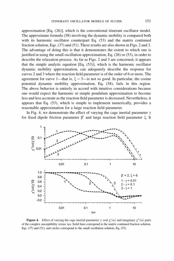
In Fig. 4, we demonstrate the effect of varying the cage inertial parameter gfor fixed dipole friction parameter b0 and large reaction field parameter x. It

0.01 0.1 1 10

−0.2

0.0

0.20.4

0.6

0.8

1.0

321

0.01 0.1 1 10

0.01

0.1

1

3

2

1

1 - γ = 0.012 - γ = 0.13 - γ = 1

β′ = 2, ξ = 6

χ′(ω

)/χ′

(0)

χ′′(ω

)/χ′

(0)

ηω

Figure 4. Effect of varying the cage inertial parameter g: real w0ðoÞ and imaginary w00ðoÞ parts

of the complex susceptibility versus Zo. Solid lines correspond to the matrix continued fraction solution,

Eqs. (37) and (51); and circles correspond to the small oscillation solution, Eq. (53).


appears that if g < 1, then the small oscillation approximation given by of

Eq. (53) again provides a very close approximation to the exact solution based

on numerical evaluations of Eqs. (37) and (51). The approximate Eq. (53)

begins to fail at g ¼ 1 and higher. This is to be expected because one is now

dealing with the region in which the Rocard approximation for the complex

susceptibility is no longer valid.

In Fig. 5, we fix the cage inertial parameter and the reaction field parameter

and we demonstrate the effect of varying the dipole friction parameter b0 for a

reasonably high value of the reaction field parameter so that one can expect the

harmonic approximation of Eq. (53) to be valid. Again the agreement with the

exact cosine potential solution, Eqs. (37) and (51), is good for relatively high

values of b0 (see curves 2 and 3). For relatively small values of b0, however,

there is some discrepancy in the intermediate frequency region. At high

frequencies the harmonic approximation, Eq. (53), cannot predict the comb-like

peak structure of the exact solution. (The peaks occur at the harmonics of the

fundamental frequency.) This to be expected because Eq. (53) results from an

expansion of the correlation function, Eq. (26) (a double transcendental function

10−4 10−3 10−2 10−1 100 101

10−4

10−4

10−3

10−3

10−2

10−2

10−1

10−1

100

100

101

−0.5

0.0

0.5

1.0

321

3

2

1

1 - β′ = 0.12 - β′ = 13 - β′ = 10 γ = 0.01, ξ = 6

χ′(ω

)/χ′

(0)

χ′′(ω

)/χ′

(0)

Figure 5. Effect of varying the dipole friction parameter b0: real w0ðoÞ and imaginary w00ðoÞparts of the complex susceptibility vs Zo. Solid lines correspond to the matrix continued fraction

solution, Eqs. (37) and (51); and circles correspond to the small oscillation solution, Eq. (53).


with sines and cosines in its argument), which is truncated at the fundamental

frequency term so that the comb-like structure may not be reproduced. Never-

theless, Eq. (53) provides a reasonable description of the fundamental frequency

peak in the FIR region as is obvious by inspection of Fig. 5. We remark that a

similar comb-like structure occurs in the theory of ferromagnetic resonance [39]

0.01 0.1 1 10

0.1

1

10T = 193 K

ƒ (THz)

0.01 0.1 1 10

0.1

1

T = 253 K

0.01 0.1 1 10

0.1

1

T = 293 K

β′ = 1.9γ = 0.035ε0-ε∞ = 9.8

β′ = 1.8γ = 0.06ε0-ε∞ = 7.6

β′ = 3.8γ = 0.01ε0-ε∞ = 14.95

ε′′(ƒ

)

Figure 6. Dielectric loss e00ðf Þ versus frequency f (f ¼ o/2p). Solid lines correspond to the

matrix continued fraction solution, Eqs. (37) and (51); and circles are experimental data for the

symmetrical top molecule CH3Cl [14,21] (Ir ¼ 28.5 10�40 g �cm2 and x ¼ 193x0=T with x0 ¼ 8).


of single-domain ferromagnetic particles, which involves the solution of

differential recurrence relations resembling Eq. (35), and in the theory of

quantum noise in ring laser gyroscopes [40].

Figure 6 shows a comparison of typical experimental data for the symmetric

top molecule CH3Cl with the theoretical spectrum predicted by Eqs. (37) and

(51). It appears that the model provides a reasonable description of both the

microwave and far-infrared spectra for this species with a fair description of the

temperature dependence.

F. Conclusions

We have shown in this section how the equations of motion of the cage model of

polar fluids originally proposed by Hill may be solved exactly using matrix

continued fractions. Furthermore, these equations automatically lead to (a) a

microwave absorption peak having its origin in the reorientational motion of the

cage and (b) a pronounced far-infrared absorption peak having its origin in the

oscillations of the dipole in the cage–dipole interaction potential. The equations

of motion of dipole and cage may be justified in terms of a generalization of the

Onsager model of the static susceptibility of polar fluids to include the dynamical

behavior. A conclusion that may be drawn from this is that the origin of the Poley

absorption peak is the interaction between the dipole and its surrounding cage

of neighbors which causes librations of the dipole. The model appears to

reproduce satisfactorily the main features of the microwave and far-infrared

absorption of CH3Cl. In addition, it is shown that the simple closed-form

expression, Eq. (53), for the complex susceptibility which was originally derived

in the context of the small oscillation version of the cage model (that is the

itinerant oscillator model) can also provide a reasonable approximation to the

susceptibility for large values of the reaction field parameter.

The result given here may also be extended to rotation in space. As far as the

cage motion is concerned, the complex susceptibility will still be governed by

the Rocard equation because the equations of motion factorize. However, the

solution for the dipole correlation function is much more complicated because

of the difficulty of handling differential recurrence relations pertaining to

rotation in space in the presence of a potential.

We remark that activation processes that involve crossing of the encaged

dipole over an internal potential barrier may also be incorporated into the

present model by adding a cos 2y term to the potential in Eq. (15). This may

give rise to a Debye-like relaxation process at very low frequencies with

relaxation time governed by the Arrhenius law, the prefactor of which may be

calculated precisely using the Kramers theory of escape of particles over

potential barriers (see Section III). We remark that a cos 2y term in the potential

has also been considered by Polimeno and Freed [41] in their discussion of a

many-body stochastic approach to rotational motions in liquids. Their


discussion is given in the context of a simplified description of a liquid in which

only three bodies are retained, namely, a solute molecule (body 1), a slowly

relaxing local structure or solvent cage (body 2), and a fast stochastic field as a

source of fluctuating torque. In general, one may remark that this approach

which is based on projection operators and numerical solution of many body

Fokker–Planck–Kramers equations is likely to be of much interest in the context

of the extension of the model described in this review to rotation in space.

Yet another direction in which the present model may be extended is

fractional dynamics where one supposes that the surroundings of the dipole or

cage obeys not the simple Langevin equation, Eq. (14), but instead a generalized

Langevin equation [13,14] with a memory function given by the Riemann–

Liouville fractional derivative [13] while Eq. (15) remains a conventional (or if

one prefers also a fractional) Langevin equation. In this way it will be possible

to incorporate slow relaxation effects into the cage model as we demonstrate in

Section IV.

III. APPLICATION TO FERROFLUIDS

We have mentioned in the general introduction that a long-standing problem in

the theory of magnetic relaxation of ferrofluids is how the solid-state or Neel

mechanism of (longitudinal) relaxation of internal rotation of the magnetic

dipole moment with respect to the crystalline axes inside the particle, the

associated transverse modes [which may give rise to ferromagnetic resonance

(FMR)], and the mechanical Brownian relaxation due to physical rotation of

the ferrofluid particle in the carrier fluid may be treated in the context of a single

model comprising both relaxation processes. (We recall that the slowest mode of

the longitudinal relaxation process describes the reversal of the magnetization

over the potential barrier created by the internal anisotropy of the particle, which

of course will be modified by an external applied field. The time to cross the

barrier is known as the Neel relaxation time and follows the Arrhenius law.)

We have mentioned that the question posed above was answered in part by

Shliomis and Stepanov [9]. They showed that for uniaxial particles, for weak

applied magnetic fields, and in the noninertial limit, the equations of motion of

the ferrofluid particle incorporating both the internal and the Brownian

relaxation processes decouple from each other. Thus the reciprocal of the

greatest relaxation time is the sum of the reciprocals of the Neel and Brownian

relaxation times of both processes considered independently—that is, those of a

frozen Neel and a frozen Brownian mechanism! In this instance the joint

probability of the orientations of the magnetic moment and the particle in the

fluid (i.e., the crystallographic axes) is the product of the individual probability

distributions of the orientations of the axes and the particle so that the

underlying Fokker–Planck equation for the joint probability distribution also


factorizes as do the statistical moments. Thus the internal and Debye processes

are statistically independent. If the applied field is sufficiently strong, however,

no such decoupling can take place.

The Shliomis–Stepanov approach [9] to the ferrofluid relaxation problem,

which is based on the Fokker–Planck equation, has come to be known in the

literature on magnetism as the egg model. Yet another treatment has recently

been given by Scherer and Matuttis [42] using a generalized Lagrangian

formalism; however, in the discussion of the applications of their method, they

limited themselves to a frozen Neel and a frozen Brownian mechanism,

respectively.

Here, we reexamine the egg model (which is of course a form [24] of the

itinerant oscillator model) noting the ratio of the free Brownian diffusion

(Debye) time to the free Neel diffusion time and discarding the assumption of a

weak applied field [12]. The results will then be used to demonstrate how the

ferrofluid magnetic relaxation problem in the noninertial or high mechanical

friction limit is essentially similar to the Neel relaxation in a uniform magnetic

field applied at an oblique angle to the easy axis of magnetization [44–48].

Unlike in the solid-state mechanism, however, the orientation of the field with

respect to the easy axis is now a function of the time due to the physical rotation

of the crystallographic axes [9] arising from the ferrofluid. The fact that the

behavior is essentially similar in all other respects to the solid-state oblique field

problem suggests that a strong intrinsic dependence of the greatest relaxation

time on the damping (independent of that due to the free diffusion time) aris-

ing from the coupling between longitudinal and transverse modes occurs.

Alternatively, the set of eigenvalues that characterize the longitudinal relaxation

now depends strongly on the damping, unlike in axial symmetry. This

precession-aided (so called because the influence of the precessional term is

proportional to the inverse of the damping coefficient) longitudinal relaxation is

absent in the weak field case [9]. Here the equations of motion decouple into

those describing a frozen Neel (pure Debye or Brownian) and a frozen

Brownian (pure Neel) mechanism of relaxation, respectively. Thus the Neel or

longitudinal relaxation is governed by an axially symmetric potential. Hence no

intrinsic dependence of the greatest relaxation time on the damping exists.

Moreover, the longitudinal set of eigenvalues is independent of the damping,

with the damping entering [48,49] via the free (Neel) diffusion time only. It

follows that in the linear response to a weak applied field, the only effect of the

fluid carrier is to further dampen, according to a Debye or Rocard (inertia-

corrected Debye) [21] mechanism, both the longitudinal and transverse

responses of the solid-state mechanism. Furthermore, it will be demonstrated

that in this case the transverse relaxation process in the ferrofluid, which may

give rise to ferromagnetic resonance, may be accurately described by the solid-

state transverse result for axial symmetry because the Brownian relaxation time


greatly exceeds the characteristic relaxation times of all the transverse modes.

The latter conclusion is reinforced by the favorable agreement of the linear

response result with experimental observations [12] of the complex suscept-

ibility of four ferrofluid samples, which is presented in Section III.E.

In order to illustrate how precession-aided relaxation effects may manifest

themselves in a ferrofluid, it will be useful to briefly summarize the differences

in the relaxation behavior for axially symmetric and nonaxially symmetric

potentials of the magnetocrystalline anisotropy and applied field, when the

Brownian relaxation mode is frozen. Thus only the solid-state (Neel) mechan-

ism is operative; that is, the magnetic moment of the single-domain particle may

reorientate only with respect to the crystalline axes.

A. Langevin Equation Formalism

Our starting point is the Landau–Lifshitz or Gilbert (LLG) equation for the

dynamics of the magnetization M of a single-domain ferromagnetic particle,

namely [48–51],

2 tN

d

dtM ¼ bða�1Ms½M H þ ½½M H MÞ ð68Þ

where

tN ¼ bð1 þ a2ÞMs

2gað69Þ

is the free diffusion time (Neel diffusion time) of the magnetic moment (solid-

state mechanism), a is the dimensionless damping (dissipation) constant, Ms is

the saturation magnetization, g is the gyromagnetic ratio, b ¼ vm=ðkTÞ, vm is the

volume (domain volume) of the particle, and a�1 determines the magnitude of

the precession term. The magnetic field H consists of applied fields (Zeeman

term), the anisotropy field Ha, and a random white noise field accounting for the

thermal fluctuations of the magnetization of an individual particle.

Equation (68) is the Langevin equation of the solid-state orientation process

[48–51]. The field H may be written as

H ¼ Hef þ HnðtÞ ð70Þ

Here

Hef ¼ � qV

qM¼ � qU

qmð71Þ


is the conservative part of H, which is determined from the free energy density V

(U is the free energy, m ¼ Msvm is the magnitude of the magnetic moment m of

the single domain particle.) The random field Hn(t) [50] has the properties [the

angular braces denote the statistical average over the realizations of Hn(t)]:

hHnðtÞi ¼ 0 ð72Þ

hHðiÞn ðtÞHð jÞ

n ðt0Þi ¼ 2kTagMsvm

dijdðt � t0Þ ð73Þ

Here dij is Kronecker’s delta; i, j ¼ 1,2,3 correspond to Cartesian (the crystalline)

axes, d(t) is the Dirac delta-function. The random variable Hn(t) must also obey

Isserlis’s theorem [21]. By introducing [9] the dipole vector

e ¼ M

Ms

¼ m

mð74Þ

we find that Eq. (68) becomes

de

dt¼ g

1 þ a2ðe HÞ þ ag

1 þ a2ðe HÞ e ð75Þ

Equation (75) has the form [21] of a kinematic relation involving the angular

velocity xe of the dipole vector e:

de

dt¼ xe e ¼ ðxL þ xRÞ e ð76Þ

Here

xL ¼ � gH

1 þ a2¼ � gðHef þ HnðtÞÞ

1 þ a2ð77Þ

is the angular velocity of free (Larmor) precession of m in the field Hef,

superimposed on which is the rapidly fluctuating Hn(t) and

xR ¼ ga1 þ a2

ðe HÞ ð78Þ

is the relaxational component of xe. Equations (77) and (78) differ from Eqs. (8)

and (9) of Shliomis and Stepanov [9] because they contain the noise field [51]

and the factor ð1 þ a2Þ�1, since the Gilbert equation is used rather than the

Landau–Lifshitz equation. The kinematic relation, Eq. (76), and the coupled

Langevin equations, Eqs. (77) and (78), are stochastic differential equations


describing the motion of the dipole vector e relative to the crystallographic

axes that is the internal or solid state relaxation. Differential recurrence relations

(equivalent to the Fokker–Planck equation) for the statistical moments governing

the dynamical behavior of e may be deduced from Eqs. (76)–(78) as described in

Refs. 21 and 34, 45–47. If we now, following Ref. 9 and allowing for the factor

(1 þ a2), introduce the magnetic viscosity

m ¼ Ms

6agð1 þ a2Þ ð79Þ

Eq. (78) becomes

6mvmxR ¼ �m qU

qmþ m HnðtÞ ð80Þ

Equation (80) will be the key equation in our discussion of precession aided Neel

relaxation.

B. Precession-Aided Effects in Neel Relaxation

The discussion given above holds for arbitrary free energy U. We now specialize

our discussion to a particle with uniaxial anisotropy, so that

vmVðMÞ ¼ U ¼ �mH0ðe � hÞ � Kvmðe � nÞ2 ð81Þ

h ¼ H0

H0ð82Þ

H0 is the amplitude of the external uniform magnetic field (the polarizing field),

K > 0 is the constant of the effective magnetic anisotropy, and n is a unit vector

along the easy magnetization axis. The fact that h is not necessarily parallel to nmeans that the axial symmetry characteristic of uniaxial anisotropy will be

broken. Thus Eq. (80) becomes

6mvmxR � mH0½e h � 2Kvmðe � nÞ½e n ¼ m HnðtÞ ¼ kRðtÞ ð83Þ

say. Next we write U explicitly as

U ¼ �mH0 cos�þ Kvm sin2 # ð84Þ

where

cos� ¼ cos#0cos#þ sin# sin#0 cos ðj� j0Þ ð85Þ


Here # and j are the polar angles of e with respect to the easy axis, which is the

polar axis: #0 and j0 are the polar angles of the external field direction h (again

with respect to the easy axis) which in the solid-state problem are constants

independent of the time. Analytic expressions for the greatest relaxation time t in

the bistable potential given by Eq. (84) in the intermediate to high damping case

(IHD) (where a is such that the energy loss per cycle of the motion of the

magnetization at the saddle point energy trajectory, �E � kT) may be obtained

using Langer’s theory [51,52] of the decay of metastable states applied to the

two-degree-of-freedom system specified by # and j, since in the solid-state case

#0 and j0 are fixed. Likewise, the Kramers energy controlled diffusion method

[51,53] may be used to obtain t in the very low damping (VLD) case where

�E � kT .

We summarize as follows [54]. The free energy vmVðMÞ, Eq. (81), has a

bistable structure with minima at n1 and n2 separated by a potential barrier

containing a saddle point [54] at n0. If ðaðiÞ1 ; aðiÞ2 ; aðiÞ3 Þ denote the direction

cosines of M and M is close to a stationary point ni of the free energy, then

VðMÞ can be approximated to second order in aðiÞ as [51,54]

V ¼ Vi þ1

2½cðiÞ1 ðaðiÞ1 Þ2 þ c

ðiÞ2 ðaðiÞ2 Þ2 ð86Þ

The relevant Fokker–Planck equation may then be solved near the saddle point,

yielding [51,54]

t ¼ tIHD � �0

2po0

½o1ebðV1�V0Þ þ o2ebðV2�V0Þ� ��1

ð87Þ

(equations for the expansion coefficients cð jÞi and Vi for the potential given by

Eq. (84) are given elsewhere [51,54]);

o21 ¼ g2M�2

s cð1Þ1 c

ð1Þ2 ; o2

2 ¼ g2M�2s c

ð2Þ1 c

ð2Þ2 ; o2

0 ¼ �g2M�2s c

ð0Þ1 c

ð0Þ2 ð88Þ

are the squares of the well and saddle angular frequencies, respectively, and

�0 ¼ b4tN

�cð0Þ1 � c

ð0Þ2 þ

ffiffiffiffiffiffiffiffiffiffiffiffiffiffiffiffiffiffiffiffiffiffiffiffiffiffiffiffiffiffiffiffiffiffiffiffiffiffiffiffiffiffiffiffiffiffiffiffiffiffiffiffiffiffiðcð0Þ2 � c

ð0Þ1 Þ2 � 4a�2c

ð0Þ1 c

ð0Þ2

q� �ð89Þ

Equation (89) is effectively the smallest positive (unstable barrier crossing mode)

eigenvalue of the noiseless Langevin equation [Eq. (75) omitting the Hn(t) term]

linearized in terms of the direction cosines about the saddle point. We remark

that the influence of the precessional term on the longitudinal relaxation is

represented by the a�2 term in Eq. (89). Furthermore, the relative magnitudes of


the precessional and aligning terms in the Langevin equations are determined

by a�1, so that Eqs. (87)–(89) and (90) below describe precession-aided

longitudinal relaxation.

Equation (87) applies when �E � kT (IHD). If �E � kT (VLD), we have

for the escape from a single well [48,51]

t ¼ tLD � pkT

o1�EebðV0�V1Þ ð90Þ

where �E � aVmjV0j. The IHD and VLD limits correspond to a� 1 and

a� 0.01, respectively. However, for crossover values of a (about a� 0.1),

neither Eq. (87) nor Eq. (90) yields reliable quantitative estimates. Thus a more

detailed analysis is necessary [51]. The most striking aspect of the precession-

aided relaxation is the behavior of the complex susceptibility for a small

alternating-current field superimposed on the strong field H0. This is particularly

sensitive to the longitudinal and transverse mode coupling, exhibiting a strong

dependence of the high-frequency ferromagnetic resonant modes (characterized

by xL) on the aligning (Neel) mode characterized by oR and vice versa.

Furthermore, suppression of the barrier crossing mode in favor of the fast

relaxation modes in the wells of the bistable potential given by Eq. (84) occurs if

the applied field is sufficiently strong. In terms of the differential recurrence

relations generated by the Langevin or Fokker–Planck equations by means of a

Fourier expansion in the spherical harmonics Yml ð#;jÞ, the coupling effect

manifests itself in recurrence relations inextricably mixed in the characteristic

numbers l and m, unlike in axial symmetry.

Finally, we remark on the asymptote for axial symmetry which arises if H0 is

reversed, or is applied parallel to the easy axis n. In the axially symmetric case

(H0 ¼ 0), t is given by Brown’s asymptotic expression [50] for simple uniaxial

anisotropy:

t � tN

ffiffiffip

p

2s3=2expðsÞ; s > 2 ð91Þ

where s ¼ bK. Thus, t normalized by tN unlike Eqs. (87)–(90) is independent of

a, so that the mode coupling effect completely disappears. Bridging formulas,

which illustrate how the asymptotic Eqs. (87) and (90) join smoothly onto the

asymptotic Eq. (91) in the limit of small H0 have been extensively discussed in

Ref. 51.

C. Effect of the Fluid Carrier: (i) Response to a Weak Applied Field

Let the crystallographic axes now rotate with angular velocity xn corresponding

to physical rotation of the ferrofluid particle due to the stochastic torques


imposed by the liquid and the aligning action of H (we now have 5 degrees of

freedom, viz., the dipole angles #, j as before and the Euler angles #0, j0, c0,which instead of being constant are now functions of the time due to the physical

rotation of the easy axis). The relative angular velocity of the dipole and easy

axis is then xR � xn, so that Eq. (83), describing the motion of m, must be

modified to

6mvmðxR � xnÞ � mH0½e h � 2Kvmðe � nÞ½e n ¼ kRðtÞ ð92Þ

The corresponding mechanical equation of motion of the particle (the particle is

treated as a rigid sphere, I is the moment of inertia of the sphere about a diameter)

is by Newton’s third law

I _xn þ 6mvmðxn � xRÞ þ 6Zvxn � 2Kvmðe � nÞ½n e ¼ knðtÞ � kRðtÞ ð93Þ

where

6Zv ¼ � ð94Þ

is the mechanical drag coefficient of the particle in the fluid, v is its hydro-

dynamic volume, and Z is the viscosity of the fluid. Thus, by addition of Eqs.

(92) and (93) we have the mechanical equation

I _xn þ 6Zvxn � mH0½e h ¼ knðtÞ ð95Þ

where the white noise knðtÞ torque arising from the fluid carrier obeys

hknðtÞi ¼ 0 ð96ÞhlðaÞn ðtÞlðbÞn ðt0Þi ¼ 2kT�dabdðt � t0Þ ð97Þ

a, b¼ 1, 2, 3 refer to the orientation of the crystallographic axes relative to

Cartesian axes fixed in the liquid. The knðtÞ again obey Isserlis’s theorem [21],

and we shall suppose that knðtÞ and kRðtÞ are uncorrelated.

Equations (92) and (95) in general are coupled to each other inextricably by

the external field term e h. If that vanishes, however, so that U depends only

on (e �n)2, they become

6mvmðxR � xnÞ � 2Kvmðe � nÞ½e n ¼ kRðtÞ ð98ÞI _xn þ 6Zvxn ¼ knðtÞ ð99Þ

The equations thus separate into the equation of motion of m relative to the easy

axis, Eq. (98), and the equation of motion of the easy axis itself, Eq. (99). The


mechanical equation, Eq. (99), is governed by two characteristic times [51]: the

Brownian diffusion or Debye relaxation time

tB ¼ 3ZvkT

ð100Þ

and the frictional time

tZ ¼ I

6Zvð101Þ

Thus the dynamical behavior of Eq. (99) is governed by the inertial parameter

(corresponding to the g of the polar fluid case of the model in Section II)

a ¼ tZtB

¼ kT

3Zv� I

6Zvð102Þ

If a ! 0, we have the noninertial response. This is treated by Shliomis and

Stepanov [9], who were able to factorize the joint distribution of the dipole and

easy axis orientations in the Fokker–Planck equation into the product of the two

separate distributions. Thus as far as the internal relaxation process is concerned,

the axially symmetric treatment of Brown [50] applies. Hence no intrinsic

coupling between the transverse and longitudinal modes exists; that is, the

eigenvalues of the longitudinal relaxation process are independent of a.

The distribution function of the easy axis orientations n is simply that of a

free Brownian rotator excluding inertial effects.

The picture in terms of the decoupled Langevin equations (98) and (99)

(omitting the inertial term I _xn in Eq. (98) is that the orientational correlation

functions of the longitudinal and transverse components of the magnetization in

the axially symmetric potential, Kvm sin2 #, are simply multiplied by the liquid

state factor, expð�t=tBÞ, of the Brownian (Debye) relaxation of the ferrofluid

stemming from Eq. (99). As far as the ferromagnetic resonance is concerned,

we shall presently demonstrate that this factor is irrelevant.

We summarize as follows: The longitudinal and transverse magnetic

susceptibilities characterizing the solid-state process are approximately des-

cribed by [55]

wjjðoÞ ¼w0jjð0Þ

1 þ iotð103Þ

w?ðoÞ ¼w0?ð0Þ½ð1 þ iot2Þ þ�

ð1 þ iot2Þð1 þ iot?Þ þ�ð104Þ

� ¼ st2

a2t2N

ðtN � t?Þ ð105Þ


In Eqs. (102) and (103), w0jjð0Þ and w0?ð0Þ are the static susceptibilities jj and ?to the easy axis and t is rendered reasonably accurately [56] by Brown’s uniaxial

anisotropy asymptote, Eq. (91), if s � 2. Furthermore, the transverse suscept-

ibility, Eq. (104), which is derived by truncating the infinite hierarchy of

differential recurrence relations for the correlation functions (with U ¼Kvm sin2 #) at the quadrupole term using the effective eigenvalue method, yields

an accurate result for the transverse response, provided that s � 5 [39]. The

effective eigenvalue solution, Eq. (104), fails [39] for s < 5 [where Eq. (91) and

Eq. (103) also cease to be entirely reliable] since at small to moderate barrier

heights a spread of the precession frequencies of the magnetization in the

anisotropy field exists. Thus the hierarchy must be solved exactly using matrix

continued fractions. In Eq. (104), t? is the effective relaxation time of the

autocorrelation functions of the components sin# cosj, sin# sinj [which are

linear combinations of the autocorrelation functions of Y11 ð#;jÞ and Y�1

1 ð#;jÞ]of the dipole moment relaxation mode, while t2 is the effective relaxation time of

the quadrupole moment relaxation mode, which is a linear combination of the

autocorrelation functions of Y12 ð#;jÞ and Y�1

2 ð#;jÞ. The effective relaxation

times t2 and t? may both be expressed [55] in terms of Dawson’s integral and

decrease monotonically with s, each having asymptotes

tN

s; s � 1 ð106Þ

Now according to linear response theory

wjj;? ¼ fjj;?ð0Þ � ioð1

0

fjj;?eiotdt ¼ ~fjj;?ð0Þ � io~fjj;?ðoÞ ð107Þ

where fjj;?ðtÞ are the longitudinal and transverse aftereffect functions, for

example,

fjjðtÞ ffi w0jjð0Þexpð�t=tÞ ð108Þ

Moreover, in the frequency domain (the tilde denoting the one-sided Fourier

transform)

~fjjðoÞ ¼w0jjð0Þ

ioþ 1=tð109Þ

~f?ðoÞ ¼w0?ð0Þ ioþ 1

t2

� �

ioþ 1t2

� �ioþ 1

t?

� �þ s

tNa21t?� 1

tN

� � ð110Þ


We note that both the effective relaxation times and the zero-frequency

susceptibilities may be written in terms of Dawson’s integral. The detailed

expressions are given in Ref. 55.

The complex susceptibility of a ferrofluid in a weak applied field may be

written directly from Eqs. (109) and (110) and the Langevin equations (98) and

(99) [taking note of Eq. (102)] using the shift theorem for one-sided Fourier

transforms, Eq. (30). Thus

wjjðoÞ ¼w0?ð0Þ

1 þ ioTjjð111Þ

with the Neel relaxation time modified to

T jj ¼ttB

tþ tB

ð112Þ

Moreover [55], provided that s is not small so that the effective eigenvalue

truncation of the hierarchy of recurrence relations for the statistical moments is

valid, we obtain

w?ðoÞ ¼w0?ð0Þ ioT2 þ 1 þ �T?T2

t?t2

h iðioT2 þ 1ÞðioT1 þ 1Þ þ �T?T2

t?t2

ð113Þ

Thus the effective relaxation time of the dipole mode is modified to

T? ¼ t?tB

t? þ tB

ð114Þ

and that of the quadrupole mode becomes

T2 ¼ t2tB

t2 þ tB

ð115Þ

In a weak measuring field the particle anisotropy axes are oriented in a random

fashion. Hence [9,57] the susceptibility (averaged over particle orientations) is

given by

w ¼ 1

3ðwjj þ 2w?Þ ð116Þ

Now [58] in ferrofluids where the Neel mechanism is blocked we have

s � 8, and so we will have in Eq. (112) t � tB; thus

T jj ffi tB ð117Þ


Furthermore, in Eqs. (114) and (115) we may use the fact [55] that t? and t2 are

monotonic decreasing functions of s and also that usually [57], for the ratio of

the free diffusion times,

tN

tB

� 10�2 ð118Þ

in order to ascertain which times may be neglected in Eq. (113). Thus we deduce

that in Eq. (113) for all s

T? ffi t? ð119ÞT2 ffi t2 ð120Þ

Hence we may conclude, recalling the exact [39] transverse relaxation solution

for w? from the Fokker–Planck equation, that the solid-state effective eigenvalue

solution embodied in Eq. (104) can also accurately describe the ferromagnetic

resonance in ferrofluids except in the range of small s (<5). Then the exact

solid-state solution based on matrix continued fractions as in Section II must be

used. The conclusion appears to be in agreement with that of Fannin [59] and

Fannin et al. [60], who have extensively analyzed experimental data on

ferrofluids using Eq. (104). By way of illustration, a detailed comparison with

experimental data for four colloidal suspensions is given in Section III.E. We

also remark that the very large s (high barrier) limit of Eq. (113) (Landau–

Lifshitz limit) agrees with the result of Scaife [58], who analyzed the problem

using an entirely different method. In the limit of high damping where a � 1,

Eq. (113) reduces to a pure relaxation equation in complete agreement with

Shliomis and Stepanov [9], namely their Eqs. (31) and (32).

Having justified how the FMR effect in ferrofluids consisting of uniaxial

particles, subjected to a weak external field, may be accurately described by the

solid-state response [that is, the factor expð�t=tBÞ arising from the mechanical

motion may be discounted in the transverse response], we shall now very briefly

describe inertial effects arising from the term I _xn in Eq. (99). Furthermore, we

shall justify the neglect of this term as far as ferrofluid relaxation is concerned.

If inertial effects are included, the correlation functions pertaining to

longitudinal and transverse motions will still be the product of the correlation

functions of the free Brownian motion of a sphere [9] and the solid-state

correlation functions hcos#ð0Þ cos#ðtÞi0, and so on; however, the composite

expressions will be much more complicated for an arbitrary inertial parameter a,

Eq. (102). The reason is that the orientational correlation functions for the

Brownian motion of a sphere may only be expressed exactly [18,19] as the

inverse Laplace transform of an infinite continued fraction in the frequency


domain. The parameter a has, however, been evaluated by Raikher and Shliomis

[57] for typical values of ferrofluid parameters and is of the order 10�5. Hence,

one may entirely neglect inertial effects unlike [21] in polar dielectrics, where

the inertial effects become progressively more important at high frequencies.

We remark that our treatment will apply not only to uniaxial anisotropy but to

an arbitrary nonaxially symmetric potential Uðe � n; tÞ of the magnetocrystalline

anisotropy. Since the potential is a function of e � n only, the autocorrelation

functions of the overall process (e.g., cubic anisotropy) will be the product of

the individual orientational autocorrelation functions of the freely rotating

sphere and the solid-state mechanism. However, unlike uniaxial anisotropy even

though the correlation functions still factorize, substantial coupling between the

transverse and longitudinal modes (which now have a dependent eigenvalues)

[cf. Eqs. (87) and (90)] will exist. The reason is that the nonaxial symmetry is

now an intrinsic property of the particles. This phenomenon should be

observable in measurements of the complex susceptibility of such particles.

D. Effect of the Fluid Carrier: (ii) Mode–Mode Coupling Effects forParticles with Uniaxial Anisotropy in a Strong Applied Field

We commence by recalling Eqs. (92) and (95). In the noninertial limit, Eq. (95)

becomes

6Zvxn � mH0½e h ¼ knðtÞ ð121Þ

and on eliminating xn in Eq. (92) with the aid of Eq. (121) we obtain

xR � mH0½e h 1

6mvm

þ 1

6Zv

� �� K

3mðe � nÞ½e n ¼ kRðtÞ

6mvm

þ knðtÞ6Zv

ð122Þ

Equation (122) is of the same form as Eq. (83) describing the motion of the

dipole moment with a frozen (Z ! 1) Brownian mechanism in the presence of

a field H0 at an oblique angle to the easy axis. It immediately follows that the

effect of the fluid on the solid-state or internal mechanism of relaxation is to alter

the magnetic drag coefficient �m of the solid-state process so that

1

�m

¼ 1

6mvm

þ 1

6Zvð123Þ

The corresponding change in the dimensionless damping coefficient a of the

solid-state process is

a0 ¼ a 1 þ mvm

Zv

� �¼ að1 þ tN=tBÞ ð124Þ


Here the ratio tN=tB represents the coupling between the magnetic and

mechanical motions arising from the nonseparable nature of the Langevin

equations, Eqs. (121) and (122). Thus the correction to the solid-state result

imposed by the fluid is once again of the order 10�2. Hence we may conclude,

despite the nonseparability of the equations of motion, that the Neel relaxation

time of the ferrofluid particle should still be accurately represented in the IHD

and VLD limits by the solid-state relaxation time formulae, Eqs. (87) and (90).

Furthermore, Eq. (122) should be closely approximated by the solid-state

relaxation equation

xR � mH0ðe hÞ 1

6mvm

� K

3mðe � nÞðe nÞ ¼ kRðtÞ

6mvm

ð125Þ

Hence, just as in the solid-state problem, one would also expect the following

effects to occur [48] in a ferrofluid for a large direct-current bias field

superimposed on which is a small alternating-current field:

(a) A strong dependence of t/tN on a (i.e., a frictional dependence of the

smallest nonvanishing eigenvalue) unlike in the weak field case (axial

symmetry), which is a signature of the coupling between the longitudinal

and transverse modes.

(b) Suppression of the Neel and barrier crossing modes in favor of the fast

relaxation modes in the deep well of the bistable potential created by

Eq. (84), if the reduced [48] bias field hc exceeds a certain critical value.

This gives rise to a high-frequency Debye-like relaxation band [43,48].

(c) A very-high-frequency FMR peak due to excitation of the transverse

modes having frequencies close to the precession frequency.

In the longitudinal response, however, guided by the relaxation time

Eq. (112), it will be necessary to have particles with t < tB so that the charac-

teristic a dependence of the response is not masked by the Brownian process

due to the damping imposed by the fluid.

We now return to the mechanical equation, Eq. (95), of motion of the

particles, which for small damping (if the small inertial term is retained)

predicts a damped oscillation of fundamental frequency [57]

o0 ¼ffiffiffiffiffiffiffiffiffiffiffiffiffiffimH0=I

pð126Þ

which would appear in the spectrum as a high-frequency resonant absorption, as

has been verified [25] in the theory of dielectric relaxation. In ferrofluids,

however, it has been estimated [57] that fields of order of magnitude 107 Oe are

needed for oscillatory effects, which is higher than any that may be obtained

under terrestrial conditions. Hence one may rule out this resonant mode of the

motion.


It remains to discuss the influence of H0 on the mechanical relaxation modes.

An estimate of this may be made by recalling that Eq. (95) is basically the

equation of motion of a rigid dipole in a strong constant external field.

Moreover, if inertial effects are neglected, it has been shown in Refs. 21 and 61

that the longitudinal and transverse effective relaxation times decrease

monotonically with field strength from tB, having asymptotic behavior

tjj �tB

x; t? � 2tB

xð127Þ

where

x ¼ vmMsH0

kT� 1 ð128Þ

Thus, the principal effect of the external field in Eq. (121) is to reduce the

Brownian relaxation time.

Since detailed experimental data for ferrofluid susceptibilities in a strong

oblique polarizing field (of intensity 10 T and higher)—superimposed on which

is a weak alternating-current field—are not yet readily available, we shall in

Section III.E confine ourselves to an illustration of how the weak alternating-

current field susceptibilities [Eqs. (111), (113), and (116), which incorporate the

effect of the fluid carrier] compare favorably with experiment. We shall also

demonstrate the effect that a weak polarizing field H0 (0–100 kA/m) has on the

susceptibility profiles (Figs. 7, 8, and 9) below. Furthermore, we shall show how

−0.4108 109

4.6 GHz1.2 GHz

0.7 GHz0.39 GHz

2.8 GHz1

12

2 3

3

fres = 0.54 GHz−0.2

0.0

0.2

0.4

0.6

0.8

1.0

1.2

χ′χ′

χ′′

χ′′

f(Hz)

Figure 7. Normalized plot of w0 and w00 against f(Hz) for samples 1, 2 and 3 over the frequency

range 100 MHz to 6 GHz.


to determine the average value of the internal field of a particle, the anisotropy

constant and the gyromagnetic ratio.

E. Comparison with Experimental Observationsof the Complex Susceptibility Data

In order to support our theoretical discussions, we now present [12] room

temperature complex susceptibility data for four colloidal suspensions, samples

1, 2, 3, and 4, respectively. The samples are as follows (in all of the samples the

surfactant is oleic acid):

Sample 1 is a 150-Gauss (0.015-T) fluid consisting of Ni0.5Zn0.5Fe2O4

particles suspended in a low-vapor-pressure hydrocarbon (isopar M). The

particles have a median diameter of 9 nm and a bulk saturation magnetization of

0.15 T.

Sample 2 is a 300-Gauss (0.03-T) fluid consisting of Mn0.66Zn0.34Fe2O4

particles suspended in isopar M. The particles have a median diameter of 9 nm

and a bulk saturation magnetization of 0.31 T.

Sample 3 is a 400-Gauss (0.04-T) fluid consisting of cobalt particles

suspended in a diester carrier. The particles have a median diameter of 7.8 nm

and a bulk saturation magnetization of 1 T.

Sample 4 is a 760-Gauss (0.076-T) fluid consisting of magnetite particles

suspended in isopar M. The particles have a median diameter of 9 nm and a bulk

saturation magnetization of 0.4 T.

108 109 1010

0.0

0.5

1.0

(b)

(b)

(a)

(a)

fres = 1.6 GHz

fmax = 1 GHz

χ′χ′

χ′′

χ′′

- data - fit

f (Hz)

Figure 8. Normalized plot of (a) w0 and w00, and (b) corresponding fits using Eqs. (111), (113),

and (116) for sample 4.


0

25

50

75

100

109

108

1010

0.0

0.5

1.0

1.5

fres = 1.6 GHz

fres = 5 GHzH (k

Am−1 )

H = 0

χ′

f (Hz)

(a)

020

40

60

80

100

108

109

1010

0.0

0.5

1.0

1.5

fmax = 4.7 GHz

fmax = 1.0 GHzH = 0

χ′′

f (Hz)

H (k

Am−1 )

(b)

Figure 9. (a) 3-D plot of w0 against f (Hz) for sample 4 over the frequency range 100 MHz to

15 GHz for 17 values of polarizing field, H0, over the range 0–100 kAm�1. (b) 3-D plot of w00 against

f(Hz) for sample 4 over the frequency range 100 MHz to 15 GHz for 17 values of polarizing field,

H0, over the range 0–100 kAm�1.


Referring to samples, 1, 2, and 3 [12], Fig. 7 shows the results obtained for

the real, w0, and imaginary, w00, susceptibility components over the frequency

range 100 MHz to 6 GHz. It is apparent that a resonant-like profile, indicated by

the w0 component changing sign, at a frequency fres, is characteristic of all

the samples. fres is seen to vary from 0.54 GHz for sample 1 to 4.4 GHz for

sample 3. As 2pfres ¼ gHA ¼ g2K=Ms (where HA and K are average values of

the particle internal field and anisotropy constant, respectively), this result is a

signature of the difference in internal field and anisotropy constant of the

particles. The susceptibility profiles have the same resonant form as that

obtained for sample 4 (see Fig. 8); these profiles are shown to have the form

predicted by Eqs. (111), (113), and (116). Furthermore, the actual values of HA

and K can be determined by means of polarized measurements as will be

demonstrated now for sample 4.

Plot (a) of Fig. 8 shows the susceptibility components obtained for sample 4

over the wider frequency range of 50 MHz to 10 GHz, while plot (b) shows the

fit obtained using Eqs. (111), (113), and (116). As magnetic fluids have a

distribution of particle shape and size, these parameters are accounted for by

modifying the above equations to include a normal distribution of anisotropy

constant, K, and a Nakagami distribution [59,60] of radii, r. Here the fit was

obtained for a mean K ¼ 1 104 J=m3 with a standard deviation of 6 103 and

a Nakagami distribution of radii, r, with a width factor b¼ 4 and a mean

particle radius r � 4:5 nm and a saturation magnetization of 0.4 T. The value

used for a, the damping parameter, was 0.1, a figure within the range of values

normally quoted [60] for a.

As far as measurements with a weak polarizing field are concerned, we

remark that variation of the polarizing field, H0, over the range 0–100 kAm�1

will result in fres increasing from 1.6 GHz to 5.0 GHz. However, a much clearer

understanding of the effect of H0 on w0 and w00 can be gleaned from a 3-D

representation of the spectra as illustrated in Fig. 9a for the w0 component and in

Fig. 9b for the w00 component. Initially, both components reduce with increasing

H0; this effect is a manifestation of the contribution of the relaxational

components to the susceptibility. Beyond approximately 400 MHz a relaxation

to resonance transition occurs with the w0 component going through zero at the

resonant frequency fres.

A plot of fres against H0 for the sample is shown in Fig. 10; and because

ores ¼ 2pfres ¼ gðH0 þ HAÞ, the value of HA is determined from the intercept

of Fig. 10 and is found to be 41 kAm�1, corresponding to a mean value

of anisotropy constant, K, at room temperature and bulk MS of 0.4 T, or 8:2 103 J/m3. The gyromagnetic ratio, g, is found to be 2:26 105 S�1 A�1 m

from the slope of Fig. 10 and is in close agreement with the theoretical value

of 2:21 105 S�1 A�1 m. Similar polarized studies undertaken [62,63]

on samples 1, 2, and 3 produced approximate HA values of 1.6, 27, and


114 kAm�1, respectively. The corresponding values of K were 120, 4 103,

and 6 104 J/m3.

F. Conclusions

The approach to the combined mechanical and magnetic motions of a ferrofluid

particle and their mutual behavior, which is based on rearrangement of the

Langevin equations and a consideration of the various characteristic time scales,

indicates how the physical effects of the fluid carrier on the magnetic relaxation

may be explained without elaborate and detailed solution (which will always

involve supermatrix continued fractions) of the various equations describing the

system. The relative orders of magnitude of the time scales involved determine

which of the existing independent internal and Brownian mode solutions may

be applied to the ferrofluid particle in any given situation. These considerations

hold even in the strong field case, where the variables cannot be separated in the

underlying Langevin equations. In particular, for zero or very weak external

fields, we have shown that the high-frequency behavior may be accurately

modeled by the solid-state result, Eq. (104), because the Brownian relaxation

time tB simply cancels out of Eq. (113) due to the relative orders of magnitude of

the various time scales. These are dictated by the ratio of the free diffusion times

and the monotonic decrease of the effective relaxation times with barrier height

that is a consequence of Dawson’s integral. This appears to be the explanation of

the success of Eq. (104) in explaining the experimental results of Section III.E

−40 −20 0 20 40 60 80 1000

1

2

3

4

5

6

H0 (kAm−1)

−41kAm−1

*109

fres (Hz)

Figure 10. Plot of fres against H0 for sample 4 in determining the average value of internal

field, HA ¼ 41 kAm�1.


and of Fannin et al. [60,62]. We further remark that no assumptions beyond that

of the effective eigenvalue truncation of the set of differential recurrence

relations have been made to obtain this result, since for zero or weak field

the Langevin equations will always decouple. Furthermore, for s < 5, where the

effective eigenvalue solution is not an accurate representation of the exact transverse

susceptibility solution [39], that solution may always be found from the under-

lying set of differential recurrence relations by using matrix continued fractions.

The experimental data on the linear response—that is, the weak a.c. field

susceptibility and the effect of a weak polarizing field, which we have presented

in Section III.E—strongly support our conjectures concerning the application of

the solid-state transverse response result, Eq. (104), to magnetic fluids.

Finally, although the equations of motion do not separate in a strong bias

field, it has been shown by considering the ratio of the free diffusion times that

the relaxation behavior is essentially similar to the Neel relaxation in an oblique

field. Thus, because all the eigenvalues now depend strongly on the damping,

one would expect various precession-aided relaxation and resonant effects to

appear in ferrofluids just as in the solid state. The precession-aided relaxation is

also of interest in connection with the stochastic resonance phenomenon

[64,65]. This phenomenon automatically appears in bistable potentials such

as Eq. (84) and should be acutely sensitive to the magnitude and direction of

the bias field because of the depletion effect produced by such a field in the

shallower of the two wells of the potential [66–69]. The stochastic resonance

effect should also be acutely sensitive to the weak alternating-current field if

the bias field is near to the critical value at which the switchover of the greatest

relaxation time from Arrhenius-like to non-Arrhenius-like behavior takes place.

In conclusion, we remark that a detailed review of matrix continued fraction

methods for the solution of differential recurrence relations is available in

Ref. 70, while a detailed account of the rotational Brownian motion of the

sphere is available in Ref. 33.

IV. ANOMALOUS DIFFUSION

The theory of the Brownian motion on which the itinerant oscillator model is

based is distinguished by a characteristic feature, namely, the concept of a

collision rate which is the inverse of the time interval between successive

collision events of the Brownian particle with its surroundings. In the words of

Einstein [71]:

We introduce a time interval t in our discussion, which is to be very small

compared with the observed interval of time, but, nevertheless of such a magnitude

that the movements executed by a particle in two consecutive intervals of time tare to be considered as mutually independent phenomena.


This concept, which is based on a random walk with a well-defined

characteristic time and which applies when collisions are frequent but weak

[13], leads to the Smoluchowski equation for the evolution of the concentration

of Brownian particles in configuration space. If inertial effects are included

(see Note 8 of Ref. 71, due to Furth), we obtain the Fokker–Planck equation for

the evolution of the distribution function in phase space which describes normal

diffusion.

On the other hand, in continuous-time random walks [13], on which the

theory of anomalous diffusion is based, the concept of a collision rate does not

hold and so the mean of the time intervals between successive collision events

diverges. Furthemore, since no characteristic time scale exists for such problems

[13], the number of collisions in a time internal (0, t) is not proportional to t for

large times. In other words the central limit theorem [21] (law of large numbers)

is no longer valid, leading to non-normal behavior. In order to describe such

anomalous diffusion processes, Barkai and Silbey [13] consider a ‘‘Brownian’’

test particle that moves freely in one dimension and that collides elastically at

random times with particles of the heat bath which are assumed to move much

more rapidly than the last particle. The times between collision events are

assumed to be independent identically distributed random variables implying

that the number of collisions is a time interval (0, t) is a renewal process. This is

reasonable according to Barkai and Silbey when the bath particles thermalize

rapidly and when the test particle is slow. Thus the time intervals between

collision events ftigare described by a probability density ðtÞ, which is

independent of the mechanical state of the test particle. Hence [13] the process

is characterized by free motion with constant velocity for a time t1, then an

elastic collision with a bath particle, then a free motion evolution for a time

ft2g, then again a collision. The most important assumption of the model is that

ðtÞ decays as a power law for long times, namely that

ðtÞ � t�1�a ð129Þ

with 0 < a < 1.

Now the mean time between collisions diverges; that is,

ð10

tðtÞ dt ! 1 ð130Þ

The above stochastic collision model then leads to a generalization of the

Fokker–Planck equation for the evolution of the phase distribution function for

mechanical particles [51] known as the fractional Klein–Kramers equation

where the velocities acquire a fractional character [13]. We shall now describe

how this equation may be used in the context of rotational Brownian motion. As


an example we will consider the dielectric relaxation of a rotator without

an external potential which would describe, for example, the motion of the

surroundings in the itinerant oscillator model. Following Ref. 72, we shall now

spend a little time to describe the application of continuous time random walks

in rotational relaxation.

A. Application of Continuous-Time Random Walksin Rotational Relaxation

Relaxation functions for fractal random walks are fundamental in the kinetics of

complex systems such as liquid crystals, amorphous semiconductors and

polymers, glass forming liquids, and so on [73]. Relaxation in these systems

may deviate considerably from the exponential (Debye) pattern. An important

task in dielectric relaxation of complex systems is to extend [74,75] the Debye

theory of relaxation of polar molecules to fractional dynamics, so that empirical

decay functions—for example, the stretched exponential of Williams and Watts

[76]—may be justified in terms of continuous-time random walks.

We have remarked earlier that a marked deficiency of the Debye theory is

that it cannot describe the dielectric relaxation process at short times [of the

order of the characteristic decay time of the dipole angular velocity correlation

function] or at high frequencies (in the FIR region) because, like the Einstein

theory of the translational Brownian motion [21], it is based on the

Smoluchowski equation. The approximate equation describing the evolution

of the probability density function (p.d.f.) of the orientations of the dipoles in

configuration space [51] is only valid when dipole inertial effects are negligible

because it assumes instantaneous equilibrium of the angular velocities. Thus the

Debye theory predicts infinite integral absorption.

We have seen that the incorporation of such inertial effects in the Debye

theory, ensuring a return to optical transparency at high frequencies, was first

achieved by Rocard [77] and a completely rigorous treatment was given by

Gross [18] and Sack [19]. They used the Klein–Kramers equation applied

to rotational Brownian motion, describing the evolution of the p.d.f. in

configuration-angular velocity space. Hence they obtained exact expressions for

the complex susceptibility of noninteracting rigid dipoles as infinite continued

fractions. The simple relaxation equation of Rocard [77] then appears for small

inertial effects—that is, where the ratio of the characteristic relaxation time of

the angular velocity correlation function to to the (Debye) relaxation time t of

the dipole relaxation function is small.

B. The Fractional Klein–Kramers Equation

In the introduction we have seen that Barkai and Silbey [13] have proposed

recently a generalization of the Klein–Kramers equation for the inertia corrected


translational Brownian motion to fractional dynamics. Here we demonstrate

how a similar fractional Klein–Kramers equation (FKKE) for the anomalous

rotational diffusion may be solved using the generalized integration theorem [73]

of Laplace transformation yielding the exact complex dielectric susceptibility in

continued fraction form as in the normal Brownian motion. The method may also

be obviously extended to all problems where solutions of the Klein–Kramers, or

more generally the Fokker–Planck equation, may be expressed as recurrence

relations involving ordinary or matrix continued fractions. Thus the itinerant

oscillator model may also be solved in fractional dynamics.

We illustrate by considering the simplest microscopic model of dielectric

relaxation, namely, an assembly of noninteracting rigid dipoles of moment meach rotating about a fixed axis through its center. This system would then

represent the motion of the cage in the itinerant oscillator model. As usual, a

dipole has moment of inertia I and is specified by the angular coordinate f so

that it constitutes a system of 1 (rotational) degree of freedom. The FKKE for

the p.d.f. Wðf; _f; tÞ in the phase space ðf; _fÞ is identical to that of the one-

dimensional translational Brownian motion of a particle [13]; however,

rotational quantities (angle f, moment of inertia I, etc.) replace translational

ones (position x, mass m, etc.) so that [72]

dW

dt¼ qW

qtþ _f

qW

qf� mE sinf

I

qW

q _f¼ 0D1�a

t LFPW ð131Þ

where

0D1�at LFPW ¼ 0D1�a

t #bq

q _fð _fWÞ þ kT

I

q2W

q _f2

� �

is the fractional Fokker–Planck operator, k is the Boltzmann constant, T is the

temperature, b ¼ �=I; � is the viscous damping coefficient of a dipole,

# ¼ t1�a; a is the anomalous exponent [73] characterizing the fractal time

process, and t is the intertrapping time scale identified with the Debye relaxation

time �=kT (at ambient temperatures, t is of the order 10�11 sec for molecular

liquids and solutions). Thus the fractional dynamics emerges from the

competition of Brownian motion events of average duration t interrupted by

trapping events whose duration is broadly distributed in accordance with our

introduction. In writing Eq. (131) we assume that a weak uniform electric field

E applied along the initial line is suddenly switched off at time t ¼ 0 so that

linear response theory [21] may be used to describe the ensuing response. In the

absence of E, Eq. (131) describes anomalous diffusion; the value a ¼1 corresponds to normal diffusion [13]. The operator 0D1�a

t � qqt 0D�a

t in


Eq. (131) is defined in terms of the convolution (the Riemann–Liouville

fractional integral definition) [73]

0D�at Wðf; _f; tÞ ¼ 1

�ðaÞ

ðt

0

Wðf; _f; t0Þ dt0

ðt � t0Þ1�a ð132Þ

so that the fractional derivative is a type of memory function [73] or

stosszahlansatz for the Boltzmann equation underlying the Fokker–Planck

equation. We remark that a slowly decaying power-law kernel in the Riemann–

Liouville operator, Eq. (132), is typical of memory effects in complex systems.

In this context we remark that the operator 0D1�at in Eq. (131) does not act on

_f qWqf and �mEI�1sinf qW

q _f(i.e., the Liouville or conservative terms) in the

convective derivative _W so that the conventional form [51] of the Boltzmann

equation with Fokker–Planck stosszahlansatz as modified by 0D1�at is preserved.

If the fractional derivative acts on the convective term [i.e., the conservative part

of Eq. (131)], then nonphysical behavior (i.e., infinite integral absorption) of the

dielectric absorption coefficient occurs as in the Debye theory of dielectric

relaxation.

C. Solution of the FractionalKlein–Kramers Equation

We may seek a solution of Eq. (131) as in normal diffusion as

Wðf; _f; tÞ ¼ e�Z2 _f2 X1p¼�1

X1n¼ 0

cp;nðtÞeipfHnðZ _fÞ ð133Þ

where Z ¼ffiffiffiffiffiffiffiffiffiffiffiffiI=2kT

pand the HnðxÞ are the Hermite polynomials. The linearized

initial (at t ¼ 0) p.d.f. is

Wðf; _f; 0Þ � 1

2p3=2Ze�Z2 _f2

1 þ mE

kTcosf

� �ð134Þ

Straightforward manipulation [72] of the recurrence relations of the Hn leads, by

orthogonality (as in Section II), to a differential recurrence relation for the

coefficients cp;nðtÞ, which may be written for the only case of interest (since the

linear response is considered), namely, p ¼ 1:

d

dtc1;nðtÞ þ

i

2Z½2ðn þ 1Þc1;nþ1ðtÞ þ c1;n�1ðtÞ ¼ �0D1�a

t #nbc1;nðtÞ ð135Þ


On using the integration theorem of Laplace transformation as generalized to

fractal calculus [73], namely,

Lf0D1�at f ðtÞg ¼ s1�a~f ðsÞ � 0D�a

t f ðtÞjt ¼ 0 ð0 < a < 1Þs1�a~f ðsÞ ð1 � a < 2Þ

�

where ~f ðsÞ ¼ Lf f ðtÞg ¼Ð1

0e�stf ðtÞ dt, we have from Eq. (135)

½2ts þ ng02ðtsÞ1�a~c1;nðsÞ þ ig0½2ðn þ 1Þ~c1;nþ1ðsÞ þ ~c1;n�1ðsÞ ¼ c1;nð0Þ ð136Þ

Here g0 ¼ t=Z ¼¼ �ffiffiffiffiffiffiffiffiffiffiffiffi2=IkT

pis chosen as the inertial effects parameter

(g0 ¼ffiffiffiffiffiffiffiffi2=g

pis effectively the inverse square root of the parameter g used earlier

in Section I). Noting the initial condition, Eq. (134), all the c1;nð0Þ in Eq. (136)

will vanish with the exception of n ¼ 0. Furthermore, Eq. (136) is an example of

how, using the Laplace integration theorem above, all recurrence relations

associated with the Brownian motion may be generalized to fractional dynamics.

The normalized complex susceptibility wðoÞ ¼ w0ðoÞ � iw00ðoÞ is given by linear

response theory as

wðoÞ ¼ wðoÞw0ð0Þ ¼ 1 � io

~c1;0ðioÞc1;0ð0Þ

ð137Þ

where w0ð0Þ ¼ m2N=ð2kTÞ and N is the number of dipoles per unit volume. [We

remark that ~c1;0ðsÞ also yields the Laplace transform of the characteristic

function of the configuration space p.d.f.]

Equation (136), which is a three-term algebraic recurrence relation for the

~c1;nðsÞ, can be solved in terms of continued fractions [21], thereby yielding the

generalization of the familiar Gross–Sack result [18,19] for a fixed axis rotator

to fractional relaxation, namely,

wðoÞ ¼ 1 � BðiotÞs

BðiotÞs þ B

1 þ BðiotÞs þ 2B

2 þ BðiotÞs þ 3B

3 þ � � �

ð138Þ

where s ¼ 2 � a and B ¼ 2g0�2ðiotÞ2ða�1Þ. Equation (138), in turn, can be

expressed in terms of the confluent hypergeometric (Kummer) function

Mða; b; zÞ [78], namely,

wðoÞ ¼ 1 � ðitoÞs

1 þ ðitoÞs Mð1; 1 þ B½1 þ ðitoÞs;BÞ ð139Þ


Equation (139) can readily be derived by comparing Eq. (138) with the continued

fraction

Mða; b; zÞðb � 1ÞMða � 1; b � 1; zÞ ¼

1

b � 1 � z þ az

b � z þ ða þ 1Þzb þ 1 � z þ � � �

ð140Þ

with a ¼ 1, z ¼ B, and b ¼ 1 þ B½1 þ ðitoÞs and by noting that

Mð0; b � 1; zÞ ¼ 1 [78]. The continued fraction, Eq. (140), can be obtained

from the known recurrence relation [78]

bð1 � b þ zÞMða; b; zÞ � azMða þ 1; b þ 1; zÞ þ bðb � 1ÞMða � 1; b � 1; zÞ ¼ 0

We remark that Mð1; 1 þ b; zÞ ¼ bz�bezgðb; zÞ, where gðb; zÞ ¼Ð z

0e�ttb�1 dt is

the incomplete gamma function [78].

For s ¼ 1, Eq. (139) can be reduced to Sack’s result [Eq. (3.19c) of Ref. 19].

In the high damping limit (g0 � 1), Eq. (139) can be simplified, yielding the

generalization to fractional dynamics of the Rocard [21,77] equation, namely,

wðoÞ ¼ 1

1 þ ðiotÞs � 2ðot=g0Þ2ð141Þ

On neglecting inertial effects (g0 ! 1), Eq. (139) becomes

wðoÞ ¼ 1

1 þ ðiotÞs ð142Þ

that is, the result previously proposed from empirical considerations [75]. For

s ¼ 1, Eq. (142) reduces to the Debye equation.

D. Dielectric Loss Spectra

Dielectric loss spectra w00ðoÞ versus log10ðoZÞ, for various values of a and g0, are

shown in Figs. 11–13. It is apparent that the spectral parameters (the

characteristic frequency, the half-width, the shape) strongly depend on both a(which pertains to the velocity space) and g0. Moreover, the high-frequency

behavior of w00ðoÞ is entirely determined by the inertia of system. It is apparent,

just as in Brownian dynamics, that inertial effects produce a much more rapid

falloff of w00ðoÞ at high frequencies. Thus the Gordon sum rule for the dipole

integral absorption of one-dimensional rotators [14,28], namely

ð10

ow00ðoÞ do ¼ pNm2

4Ið143Þ


−6 −4 −2 0 2

−4

−2

0

1′2′

3

1,1′ : α = 0.252,2′ : α = 0.53,3′ : α = 1.04,4′ : α = 1.5

4′

γ ′= 10

4

2

3′

1

log10[ηω]

log 1

0[χ′

′(ω)]

∧

Figure 11. Dielectric loss spectra w00ðoÞ for g0 ¼ 10 and various values of a: a¼ 0.25 (curves 1

and 10), a¼ 0.5 (2, 20), a¼ 1 (3, 30), and a¼ 1.5 (4, 40). Solid lines (exact solution) (1, 2, 3, and 4):

Eq. (139); crosses (10, 20, 30, and 40): Eq. (142); filled circles: Eq. (141).

0 2

0

2

5′4′

α = 0.5

5

42,2′ 3,3′1,1′

−6

−6

−4

−4

−2

−2

1,1′: γ ′ = 104

2,2′: γ ′ = 103

3,3′: γ ′ = 102

4,4′: γ ′ = 101

5,5′: γ ′ = 1

log10[ηω]

log 1

0[χ′

′(ω)]

∧

Figure 12. Dielectric loss spectra w00ðoÞ for a¼ 0.5 (enhanced diffusion) and various values of

g0: g0 ¼ 104 (curves 1 and 10), g0 ¼ 103 (2, 20), g0 ¼ 102 (3, 30), g0 ¼ 10 (4, 40), and g0 ¼ 1 (5, 50). Solid

lines (exact solution) (1, 2, 3, 4, and 5): Eq.(139); crosses (10, 20, 30, 40, and 50): Eq. (142); filled

circles: Eq. (141).


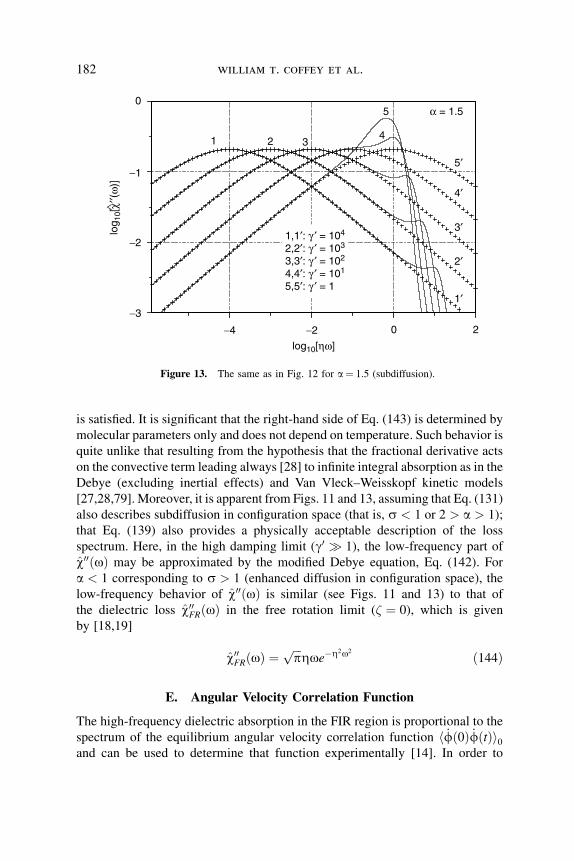
is satisfied. It is significant that the right-hand side of Eq. (143) is determined by

molecular parameters only and does not depend on temperature. Such behavior is

quite unlike that resulting from the hypothesis that the fractional derivative acts

on the convective term leading always [28] to infinite integral absorption as in the

Debye (excluding inertial effects) and Van Vleck–Weisskopf kinetic models

[27,28,79]. Moreover, it is apparent from Figs. 11 and 13, assuming that Eq. (131)

also describes subdiffusion in configuration space (that is, s < 1 or 2 > a > 1);

that Eq. (139) also provides a physically acceptable description of the loss

spectrum. Here, in the high damping limit (g0 � 1), the low-frequency part of

w00ðoÞ may be approximated by the modified Debye equation, Eq. (142). For

a < 1 corresponding to s > 1 (enhanced diffusion in configuration space), the

low-frequency behavior of w00ðoÞ is similar (see Figs. 11 and 13) to that of

the dielectric loss w00FRðoÞ in the free rotation limit (� ¼ 0), which is given

by [18,19]

w00FRðoÞ ¼ffiffiffip

pZoe�Z2o2 ð144Þ

E. Angular Velocity Correlation Function

The high-frequency dielectric absorption in the FIR region is proportional to the

spectrum of the equilibrium angular velocity correlation function h _fð0Þ _fðtÞi0

and can be used to determine that function experimentally [14]. In order to

0 2

0

1′

2′

3

5′

4′

α = 1.55

42

3′

1

−3

−4

−1

−2

−21,1′: γ ′ = 104

2,2′: γ ′ = 103

3,3′: γ ′ = 102

4,4′: γ ′ = 101

5,5′: γ ′ = 1

log10[ηω]

log 1

0[χ′

′(ω)]

∧

Figure 13. The same as in Fig. 12 for a¼ 1.5 (subdiffusion).


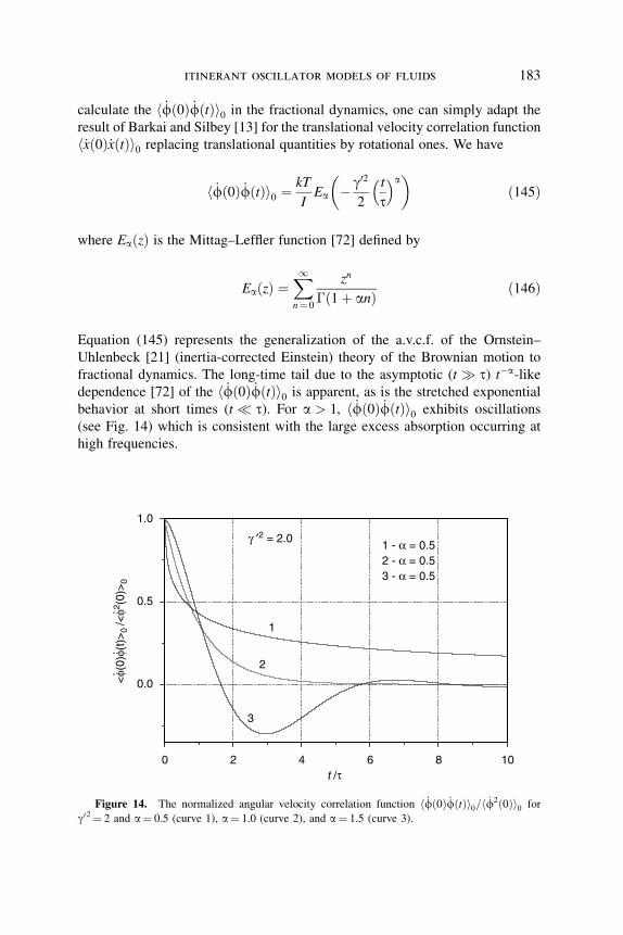
calculate the h _fð0Þ _fðtÞi0 in the fractional dynamics, one can simply adapt the

result of Barkai and Silbey [13] for the translational velocity correlation function

h _xð0Þ _xðtÞi0 replacing translational quantities by rotational ones. We have

h _fð0Þ _fðtÞi0 ¼ kT

IEa � g02

2

t

t

� �a� �

ð145Þ

where EaðzÞ is the Mittag–Leffler function [72] defined by

EaðzÞ ¼X1n¼ 0

zn

�ð1 þ anÞ ð146Þ

Equation (145) represents the generalization of the a.v.c.f. of the Ornstein–

Uhlenbeck [21] (inertia-corrected Einstein) theory of the Brownian motion to

fractional dynamics. The long-time tail due to the asymptotic (t � t) t�a-like

dependence [72] of the h _fð0Þ _fðtÞi0 is apparent, as is the stretched exponential

behavior at short times (t � t). For a > 1, h _fð0Þ _fðtÞi0 exhibits oscillations

(see Fig. 14) which is consistent with the large excess absorption occurring at

high frequencies.

0 2 4 6 8 10

0.0

0.5

1.0

γ ′2 = 2.01 - α = 0.52 - α = 0.53 - α = 0.5

3

2

1

t /τ

<φ(

0)φ(

t)>

0 /<

φ2 (0)

>0

..

.

Figure 14. The normalized angular velocity correlation function h _fð0Þ _fðtÞi0=h _f2ð0Þi0 for

g02 ¼ 2 and a¼ 0.5 (curve 1), a¼ 1.0 (curve 2), and a¼ 1.5 (curve 3).


F. Conclusions

We have demonstrated how existing Brownian motion solutions for dielectric

relaxation may be generalized to fractional dynamics using continued fractions

[21] and the Laplace transform of the Riemann–Liouville definition of the

fractional derivative. The result is of particular interest in dielectric relaxation

because it demonstrates how the unphysical high-frequency divergence of the

absorption coefficient due to the neglect of inertia may be removed in fractional

relaxation as in inertia-corrected Debye relaxation (see Figs. 11–13). The

methods we have outlined are obviously applicable on account of Eq. (132) to

other relaxation models such as the itinerant oscillator, which attempt to

incorporate both resonance and relaxation behavior in a single model with the

purpose of simultaneously explaining the Debye (low-frequency) and FIR

absorption spectra of complex dipole systems (recent applications of fractional

models to anomalous dielectric relaxation are given, e.g., in Refs. 79–83).

In passing, we finally note that possible new applications of the methods des-

cribed in this review are the fluctuations of a rubidium atom on the surface of a

fullereme cage [84] and orientation moments of spheroids in simple shear

flow [85].

Acknowledgments

The support of this work by the Enterprise Ireland Research Collaboration Fund 2001, the Trinity

College Dublin Trust, USAF, EOARD (contract F61773-01-WE407), and INTAS (project no.

01-2341) is gratefully acknowledged. W. T. C. is the holder of a Berkeley Fellowship 2001–2002 at

Trinity College Dublin for the academic year 2001–2002.

References

1. N. E. Hill, Proc. Phys. Soc. Lond. 82, 723 (1963).

2. V. F. Sears, Proc. Phys. Soc. Lond. 86, 953 (1965).

3. G. A. P. Wyllie, J. Phys. C 4, 564 (1971).

4. J. H. Calderwood and W. T. Coffey, Proc. R. Soc. Lond. A365, 269 (1977).

5. W. T. Coffey, P. M. Corcoran, and M. W. Evans, Proc. R. Soc. Lond. A410, 61 (1987).

6. W. T. Coffey, P. M. Corcoran, and J. K. Vij, Proc. R. Soc. Lond. A414, 339 (1987).

7. W. T. Coffey, P. M. Corcoran, and J. K. Vij, Proc. R. Soc. Lond. A425, 169 (1989).

8. M. I. Shliomis, Sov. Phys. Usp. 17, 153 (1974).

9. M. I. Shliomis and V. I. Stepanov, in Relaxation Phenomena in Condensed Matter, Advances in

Chemical Physics, Vol. 87, W. T. Coffey, ed., Wiley, New York, 1994, p. 1.

10. P. S. Damle, A. Sjolander, and K. S. Singwi, Phys. Rev. 165, 277 (1968).

11. N. G. van Kampen, Stochastic Processes in Physics and Chemistry, 2nd ed., North-Holland,

Amsterdam, 1992.

12. W. T. Coffey and P. C. Fannin, J. Phys. Cond. Matter 14, 1(2002).

13. E. Barkai and R. S. Silbey, J. Phys. Chem. B. 104, 3866 (2000).

14. M.W.Evans,G.JEvans,W.T.Coffey,andP.Grigolini,MolecularDynamics,Wiley,NewYork,1982.


15. W. T. Coffey, M. W. Evans, and P. Grigolini, Molecular Diffusion and Spectra, Wiley, New York

1984; Russian translation: Mir, Moscow, 1987.

16. J. P. Poley, J. Appl. Sci. B4, 337 (1955).

17. G. P. Johari, J. Non-Crystalline Solids 307, 114 (2002).

18. E. P. Gross, J. Chem. Phys. 23, 1415 (1955).

19. R. A. Sack, Proc. Phys. Soc. B 70 402, 414 (1957).

20. Dielectric Properties and Molecular Behavior, N. E. Hill, W. E. Vaughan, A. H. Price, and

M. Davies, eds., D. Van Nostrand, London, 1969, p. 90.

21. W. T. Coffey, Y. P. Kalmykov, and J. T. Waldron, The Langevin Equation, World Scientific,

Singapore, 1996, reprinted 1998.

22. P. Debye, Polar Molecules, Chemical Catalog, New York 1929, reprinted by Dover Publications,

New York, 1954.

23. G. A. P. Wyllie, in Dielectric and Related Molecular Processes, vol. 1, Specialist Periodical

Reports, Senior Reporter, M. Davies, The Chemical Society, London, 1972, p. 21.

24. W. T. Coffey, J. Chem. Phys. 107, 4960 (1997).

25. W. T. Coffey, Y. P. Kalmykov, and S. V. Titov, J. Chem. Phys. 115, 9895 (2001).

26. W. T. Coffey, J. Chem. Phys. 93, 724 (1990).

27. B. K. P. Scaife, Principles of Dielectrics, Oxford University Press, London, 1989, revised edition

1998.

28. B. K. P. Scaife, Complex Permittivity, The English Universities Press, London, 1971.

29. W. T. Coffey, C. Rybarsch, and W. Schroer, Chem. Phys. Lett. 99, 31 (1983).

30. H. Frohlich, Theory of Dielectrics, Oxford University Press, London (1958).

31. H. Frohlich, personal communication to W. T. Coffey, 1987.

32. W. T. Coffey and M. E. Walsh, J. Chem. Phys. 106, 7625 (1997).

33. J. R. McConnell, Rotational Brownian Motion and Dielectric Theory, Academic, London, 1980.

34. Yu. P. Kalmykov, J. Mol. Liq. 69, 53 (1996).

35. J. T. Waldron, Yu. P. Kalmykov, and W. T. Coffey, Phys. Rev. E 49, 3976 (1994).

36. M. E. Walsh and P. M. Dejardin, J. Phys. B 32, 1 (1998).

37. H. Mori, Prog. Theor. Phys. 33, 423 (1965).

38. E. C. Titchmarsh, An Introduction to the Theory of Fourier Integrals, Oxford University Press,

London, 1937.

39. Yu. P. Kalmykov and W. T. Coffey, Phys. Rev. B 56, 3325 (1997).

40. W. T. Coffey, Y. P. Kalmykov, and E. S. Massawe, Phys. Rev. E 48, 699 (1993).

41. A. Polimeno and J. H. Freed, Adv. Chem. Phys. 83, 89 (1993).

42. C. Scherer and H. G. Matuttis, Phys. Rev. E 63, 1 (2001).

43. W. T. Coffey, D. S. F. Crothers, J. L. Dormann, L. J. Geoghegan, and E.C. Kennedy, Phys. Rev.

B 58, 3249 (1998).

44. W. T. Coffey, D. S. F. Crothers, J. L. Dormann, Y. P. Kalmykov, E. C. Kennedy, and

W. Wernsdorfer, Phys. Rev. Lett. 80, 5655 (1998).

45. Y. P. Kalmykov and S. V. Titov, Phys. Rev. Lett. 82, 2967 (1999).

46. Y. P. Kalmykov and S. V. Titov, Phys. Solid State (St. Petersburg) 40, 1492 (1998).

47. W. T. Coffey, P. J. Cregg, and Y. P. Kalmykov, Adv. Chem. Phys. 83 263 (1993).

48. W. T. Coffey, D. S. F. Crothers, Y. P. Kalmykov, and S.V. Titov, Phys. Rev. B 64 (012411) (2001).


49. W. F. Brown, Jr., IEEE Trans. Magn. MAG-15, 196 (1979).

50. W. F. Brown, Jr., Phys. Rev. 130, 1677 (1963).

51. W. T. Coffey, D. A. Garanin, and D. J. McCarthy, Adv. Chem. Phys. 117, 483 (2001).

52. J. S. Langer, Ann. Phys. (N.Y.) 54, 258, 1969.

53. H. A. Kramers, Physica (Utrecht) 7, 284 (1940).

54. L. J. Geoghegan, W. T. Coffey, and B. Mulligan, Adv. Chem. Phys. 100, 475 (1997).

55. W. T. Coffey, Y. P. Kalmykov, and E. S. Massawe, in Modern Nonlinear Optics, Part 2, M. W.

Evans and S. Kielich, eds., Advances in Chemical Physics, Vol. 85, Wiley, New York, 1993, p.667.

56. W. T. Coffey, D. S. F. Crothers, Y. P. Kalmykov, E. S. Massawe, and J. T. Waldron, Phys. Rev. E 49,

1869 (1994).

57. Y. L. Raikher and M. I. Shliomis, in Relaxation Phenomena in Condensed Matter, W. T. Coffey,

ed., Advances in Chemical Physics, Vol. 87, Wiley, New York, 1994, p. 595.

58. B. K. P. Scaife, Adv. Chem. Phys. 109, 1 (1999).

59. P. C. Fannin, Adv. Chem. Phys. 104, 181 (1998).

60. P. C. Fannin, T. Relihan, and S. W Charles, Phys. Rev B 55, 21 (1997).

61. J. T. Waldron, Y. P. Kalmykov, and W. T. Coffey, Phys. Rev. E 49, 3976 (1994).

62. P. C. Fannin, T. Relihan, and S. W. Charles, J. Magn. Magn. Mater. 162, 319 (1996).

63. P. C. Fannin, S. W. Charles, and J. L. Dormann, J. Magn. Magn. Mater. 201, 98 (1999).

64. Y. L. Raikher and V. I. Stepanov, J. Phys. Cond. Matter 6, 4137 (1994).

65. L. Gammaitoni, P. Hanggi, P. Jung, and F. Marchesoni, Rev. Mod. Phys. 70, 223 (1998).

66. W. T. Coffey, D. S. F. Crothers, and Y. P. Kalmykov, Phys. Rev. E 55, 4812 (1997).

67. D. A. Garanin, Phys. Rev. E 54, 3250 (1996).

68. W. T. Coffey, Adv. Chem. Phys. 103, 259 (1998).

69. W. T. Coffey, D. S. F. Crothers, Y. P. Kalmykov, and J. T. Waldron, Phys. Rev. B 51, 15947 (1995).

70. J. L. Dejardin, Y. P. Kalmykov, and P. M. Dejardin, Adv. Chem. Phys. 117, 275 (2001).

71. A. Einstein. Investigations on the Theory of the Brownian Movement, R. Furth, ed., Dover

Publications, New York, 1956.

72. W. T. Coffey, Y. P. Kalmykov, and S. V. Titov, Phys. Rev. E 65, 032102 (2002).

73. R. Metzler and J. Klafter, Adv. Chem. Phys. 116, 223 (2001).

74. W. G. Glockle and T. F. Nonnenmacker, J. Stat. Phys. 71, 741 (1993).

75. K. Weron and M. Kotulski, Physica A 232, 180 (1996).

76. G. Williams and D. C. Watts, Trans. Faraday Soc. 66, 80 (1970).

77. M. Y. Rocard, J. Phys. Radium 4, 247 (1933).

78. M. Abramowitz and I. Stegun, eds., Handbook of Mathematical Functions, Dover, New York, 1964.

79. J. H. Van Vleck and V. F. Weisskopf, Rev. Mod. Phys. 17, 227 (1945).

80. R. R. Nigmatullin and Y. A. Ryabov, Fizika Tverdogo Tela (St. Petersburg) 39, 101 (1997) [Phys.

Solid State 39, 87 (1997)].

81. V. V. Novikov and V. P. Privalko, Phys. Rev. E 64, 031504 (2001).

82. W. T. Coffey, Y. P. Kalmykov, and S. V. Titov, Phys. Rev. E 65, 032102 (2002).

83. W. T. Coffey, Y. P. Kalmykov, and S. V. Titov, J. Chem. Phys. 116, 6422 (2002).

84. P. Dugourd, R. Antoine, D. Rayane, E. Benichou, and M. Broyer, Phys. Rev. A 62, 011201 (2000).

85. K. Asokan, T. R. Ramamohan, and V. Kumaran, Phys. Fluids 14, 75 (2002).

86. M. C. Wang and G. E. Uhlenbeck, Rev. Mod. Phys. 17, 323 (1945).


Itinerant Oscillator Models of Fluids

Documents

Transcript of Itinerant Oscillator Models of Fluids