1

Planar Curve Offset

Based on Circle Approximation ∗

In-Kwon Lee∗, Myung-Soo Kim∗, and Gershon Elber+

* Department of Computer Science, POSTECH, Pohang 790-784, South Korea

+ Department of Computer Science, Technion, IIT, Haifa 32000, Israel

Abstract

An algorithm is presented to approximate planar offset curves within an arbitrarytolerance ε > 0. Given a planar parametric curve C(t) and an offset radius r, the circleof radius r is first approximated by piecewise quadratic Bezier curve segments withinthe tolerance ε. The exact offset curve Cr(t) is then approximated by the convolutionof C(t) with the quadratic Bezier curve segments. For a polynomial curve C(t) ofdegree d, the offset curve Cr(t) is approximated by planar rational curves, Ca

r (t)’s, ofdegree 3d − 2. For a rational curve C(t) of degree d, the offset curve is approximatedby rational curves of degree 5d − 4. When they have no self-intersections, the approx-imated offset curves, Ca

r (t)’s, are guaranteed to be within ε-distance from the exactoffset curve Cr(t). The effectiveness of this approximation technique is demonstratedin the offset computation of planar curved objects bounded by polynomial/rationalparametric curves.

Keywords: Offset, convolution, curve approximation, hodograph, NC machining, Bezier/B-

spline curves, rational curve.

1 Introduction

Constant radius offsetting for curves and surfaces is one of the most important geometric

operations in CAD/CAM due to its immediate application to NC machining [6, 14]. At the

same time, the offsetting is one of the most difficult geometric operations to implement. The

∗Computer-Aided Design, Vol. 28, No. 8, pp. 617–630, August, 1996

exact offset curves and surfaces have very high algebraic degree compared with the original

curves and surfaces. For example, the offset of a cubic Bezier curve has algebraic degree 10

[9].

Given a planar regular parametric curve C(t) = (x(t), y(t)), the offset curve Cr(t) (with

respect to a fixed radius r) is defined by:

Cr(t) = C(t) + r ·N(t),

where

N(t) =(y′(t),−x′(t))√x′(t)2 + y′(t)2

is the unit normal of C(t). (In this paper, we assume the normal vectors of a planar curve

are pointing to the right of the curve advancing direction.) Due to the square root function

in the denominator of N(t), the exact offset curves are not rational, in general [9].

Farouki and Sakkalis [10] considered the special case of x′(t)2 + y′(t)2 = σ(t)2 for some

polynomial σ(t). These curves are called “Pythagorean hodograph curves,” and their offset

curves are rational. However, they have less degrees of freedom than other polynomial curves

with the same degree [10]. For example, a cubic Pythagorean hodograph curve has only one

degree of freedom; at least degree five is required for a Pythagorean hodograph curve to have

an inflection point. The Pythagorean hodograph curves have many useful properties which

need further investigation. Nevertheless, for the time being, approximation techniques seem

to be the only feasible practical solution to the planar curve offsetting.

Previous offset computation methods for parametric curves approximated either (i) the

original curve C(t) by line segments and circular arcs [22], or (ii) the offset curve Cr(t) by

low degree polynomial curves [3, 4, 17, 18, 19, 23, 24]. The offsets for line segments and

circular arcs are also line segments and circular arcs [22]. However, many line segments

and circular arcs are required to approximate a given planar curve. Although quadratic or

cubic curves approximate the given curve with fewer curve segments, the offset even for a

quadratic curve is not rational. The approximation method of [22] is thus limited only to

line segments and circular arcs. The other methods approximate the offset curve by spline

curve segments [3, 4, 17, 18, 19, 23, 24]. They estimate the approximation error only at

finite sample points, which may inaccurately reflect the global error. Moreover, each curve

subdivision is made at the midpoint of the curve, which may not be the optimal subdivision

point.

Elber and Cohen [6] estimated the offset approximation error by computing the maximum

value of the difference function ψ(t) = ‖Car (t)−C(t)‖2−r2, where Ca

r (t) is an approximation

of Cr(t). Curve refinement is made at the parameter value(s) which gives the maximum error.

This technique reduces the size of curve data. Any of the previous methods [3, 4, 17, 18, 19,

2

23, 24] can be used to construct the approximated offset spline curve Car (t). None of these

methods, however, guarantees that the curve Car (t) has similar speed to Cr(t). Even when the

overall traces of the two curves are close to each other, the distance ‖Car (t)−Cr(t)‖ may be

taken to be larger than the actual distance, and the error measure ψ(t) = ‖Car (t)−C(t)‖2−r2

may over-estimate the actual distance between Car and Cr. In Reference [6], the error measure

ψ(t) = ‖Car (t) − C(t)‖2 − r2 was used in conjunction with the assumption that the offset

approximation converges to the actual offset. There are, however, some special cases in

which this assumption is not valid. For example, consider the offset curve approximation

Car (t) = C(t) + (r, 0); that is, Ca

r (t) is a translation of C(t) along the x axis by an amount

of r. Clearly, the error measure ψ(t) ≡ 0; but the curve Car (t) is completely different from

the exact offset curve Cr(t). In this way, the measure may also under-estimate the error.

Elber and Cohen [6] provided a way to remedy this shortcoming; they proposed to measure

the angle between the difference vector δ(t) = Car (t) − C(t) and the unit normal vector

N(t). As a result, the distance and angle functionals in [6] bound each approximated offset

curve point within a small neighborhood of the exact offset point, and thus construct a

very precise approximated offset curve. However, it is difficult to completely eliminate error

over-estimation. All the previous methods have the same problem, the only exception being

the simplest method of [22].

Taking a slightly different approach, this paper suggests a method that measures the

actual approximation error more precisely. The planar curve offsetting problem is interpreted

as a sweeping problem in which the center of a circle of radius r is moving along the given

planar curve. The boundary of the sweep is obtained as an envelope curve of the swept circle,

which is identical to the exact offset curve [2, 13]. This envelope curve is also known as a

convolution curve. The convolution curve of two parametric curves C(t) and Q(s) is defined

as the curve C(t)+Q(s(t)), where C ′(t) and Q′(s) have the same direction at s = s(t) [2, 13].

This relationship between C ′(t) and Q′(s) requires a proper reparametrization of s = s(t)

as a function of t. To make the reparametrization easier, the moving circle is approximated

with piecewise quadratic Bezier curve segments within a tolerance ε > 0.

Let C(t) = (x(t), y(t)), t1 ≤ t ≤ t2, be a polynomial curve of degree d and Q(s) =

(xQ(s), yQ(s)), s1 ≤ s ≤ s2, be a quadratic curve. Then, Q(s) has a linear hodograph

Q′(s) = (x′Q(s), y′Q(s)) = (as + b, cs + d), for some constants a, b, c, d ∈ R. Assume the

mapping, t ∈ [t1, t2] �→ s(t) ∈ [s1, s2], is a bijection, where C ′(t) and Q′(s(t)) have the same

direction. Then, the condition of C ′(t) and Q′(s) having the same direction implies a linear

equation of s: x′(t)(cs + d) − y′(t)(as + b) = 0, where x′(t) and y′(t) are polynomials of

degree d− 1. The proper reparametrization of s = s(t) is obtained as a rational polynomial

of degree d − 1 in t. Under the reparametrization, the approximated offset circle, Q(s(t)),

is a planar rational curve of degree 2(d − 1), and the convolution curve, C(t) + Q(s(t)), is

3

Q(s)

r

r + ε

r − ε

C(t)

Car (t)Cr(t)

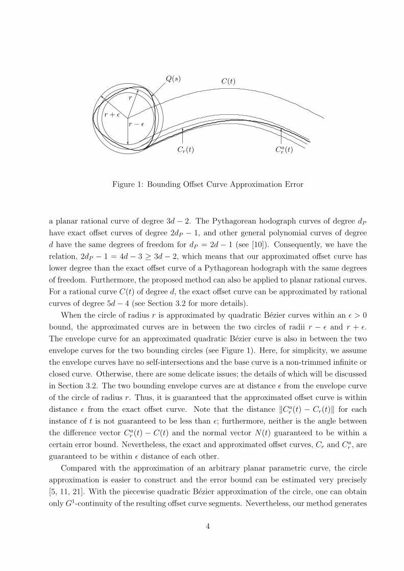
Figure 1: Bounding Offset Curve Approximation Error

a planar rational curve of degree 3d − 2. The Pythagorean hodograph curves of degree dP

have exact offset curves of degree 2dP − 1, and other general polynomial curves of degree

d have the same degrees of freedom for dP = 2d − 1 (see [10]). Consequently, we have the

relation, 2dP − 1 = 4d − 3 ≥ 3d − 2, which means that our approximated offset curve has

lower degree than the exact offset curve of a Pythagorean hodograph with the same degrees

of freedom. Furthermore, the proposed method can also be applied to planar rational curves.

For a rational curve C(t) of degree d, the exact offset curve can be approximated by rational

curves of degree 5d− 4 (see Section 3.2 for more details).

When the circle of radius r is approximated by quadratic Bezier curves within an ε > 0

bound, the approximated curves are in between the two circles of radii r − ε and r + ε.The envelope curve for an approximated quadratic Bezier curve is also in between the two

envelope curves for the two bounding circles (see Figure 1). Here, for simplicity, we assume

the envelope curves have no self-intersections and the base curve is a non-trimmed infinite or

closed curve. Otherwise, there are some delicate issues; the details of which will be discussed

in Section 3.2. The two bounding envelope curves are at distance ε from the envelope curve

of the circle of radius r. Thus, it is guaranteed that the approximated offset curve is within

distance ε from the exact offset curve. Note that the distance ‖Car (t) − Cr(t)‖ for each

instance of t is not guaranteed to be less than ε; furthermore, neither is the angle between

the difference vector Car (t) − C(t) and the normal vector N(t) guaranteed to be within a

certain error bound. Nevertheless, the exact and approximated offset curves, Cr and Car , are

guaranteed to be within ε distance of each other.

Compared with the approximation of an arbitrary planar parametric curve, the circle

approximation is easier to construct and the error bound can be estimated very precisely

[5, 11, 21]. With the piecewise quadratic Bezier approximation of the circle, one can obtain

only G1-continuity of the resulting offset curve segments. Nevertheless, our method generates

4

very precise offset curve approximation with a smaller number of curve subdivisions than the

previous methods, especially when high precision is required for the offset approximation.

(See Elber et al. [7] for more detailed comparisons of the previous methods.) Both the

precision and data reduction of our offset approximation algorithm are essentially based on

the simple error estimation, which is guaranteed to be the same as the circle approximation

error. In many practical applications of the planar curve offsetting (e.g., NC tool path

generation), the accuracy of offset curve approximation and the reduction of output data

size are two important criteria which must be considered.

This paper is organized as follows. Section 2 reviews circle approximation methods with

piecewise quadratic Bezier curve segments [5, 11, 21]. Section 3 describes an algorithm

to approximate the offset curve with rational parametric curves. Section 4 describes an

algorithm to eliminate the local and global self-intersecting loops in the offset of a planar

curved object. Section 5 demonstrates some experimental results. Finally, we conclude the

paper in Section 6.

2 Circle Approximation with Quadratic Bezier Curve

Segments

In this section, we review five different methods to approximate a unit circular arc by using

a quadratic Bezier curve segment Q(s), 0 ≤ s ≤ 1. The approximation methods are derived

in a straightforward manner from the cubic Bezier curve approximations of a circle [5, 11].

Morken [21] also developed the same circle approximations with quadratic Bezier curves.

The main contribution of Morken [21] is in proving that each method is optimal under the

given curve constraints; the optimality proof is not clear in the previous work [5, 11]. We

present the curve construction methods in detail here (without optimality proofs) since they

will be used for the construction of approximated offset curves, Car (t)’s, in the next section.

2.1 General Formulas for Quadratic Bezier Curves

The quadratic Bezier curve with three control points, P0, P1, and P2, is given by:

Q(s) = (1− s)2P0 + 2s(1− s)P1 + s2P2, for 0 ≤ s ≤ 1.

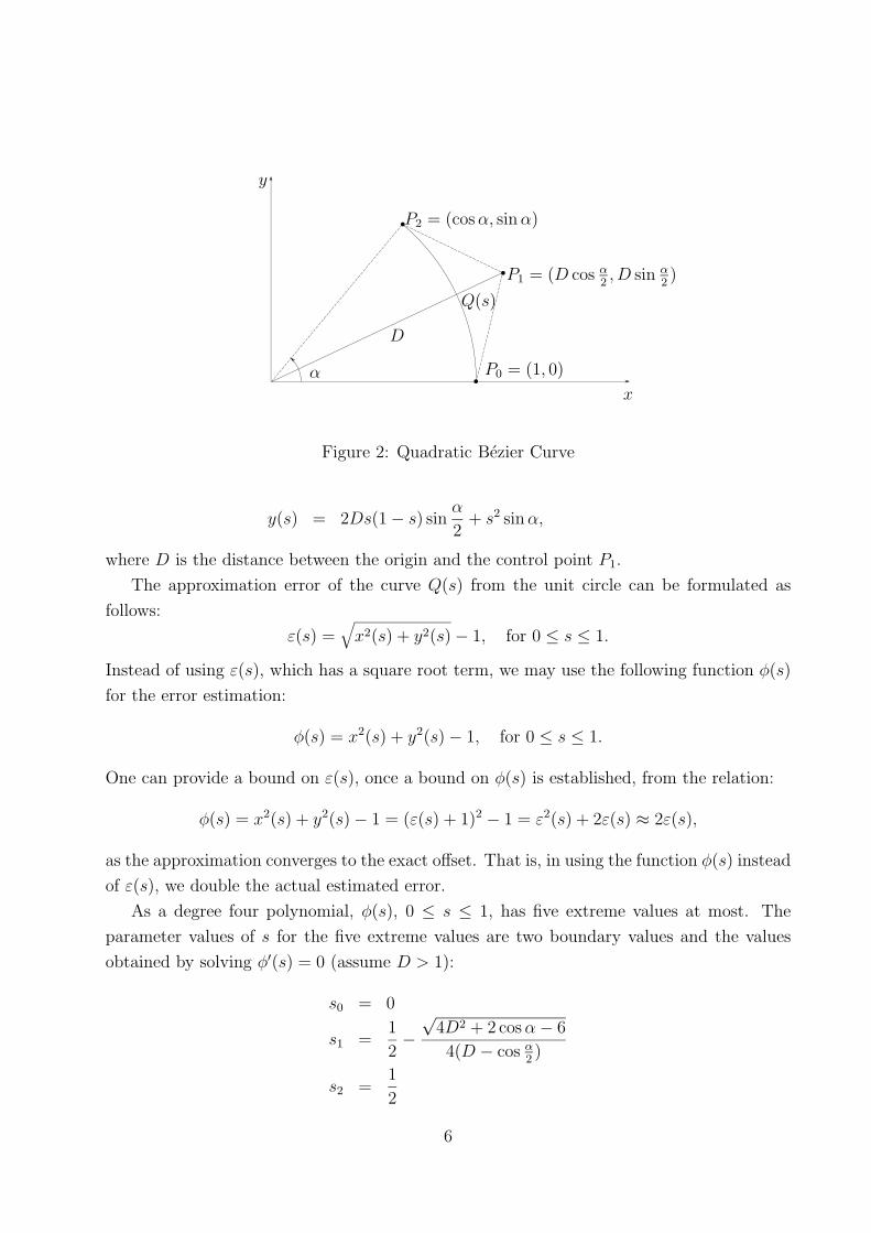
For the circle approximation, we may assume that P0 = (1, 0) and P2 = (cosα, sinα) (see

Figure 2). For the sake of simplicity, we consider only the case of α ≤ π2. The quadratic

Bezier curve Q(s) = (x(s), y(s)), 0 ≤ s ≤ 1, has the coordinate equations:

x(s) = (1− s)2 + 2Ds(1− s) cos α2+ s2 cosα,

5

α P0 = (1, 0)

P1 = (D cos α2, D sin α

2)

P2 = (cosα, sinα)

D

Q(s)

x

y

Figure 2: Quadratic Bezier Curve

y(s) = 2Ds(1− s) sin α2+ s2 sinα,

where D is the distance between the origin and the control point P1.

The approximation error of the curve Q(s) from the unit circle can be formulated as

follows:

ε(s) =√x2(s) + y2(s)− 1, for 0 ≤ s ≤ 1.

Instead of using ε(s), which has a square root term, we may use the following function φ(s)

for the error estimation:

φ(s) = x2(s) + y2(s)− 1, for 0 ≤ s ≤ 1.

One can provide a bound on ε(s), once a bound on φ(s) is established, from the relation:

φ(s) = x2(s) + y2(s)− 1 = (ε(s) + 1)2 − 1 = ε2(s) + 2ε(s) ≈ 2ε(s),

as the approximation converges to the exact offset. That is, in using the function φ(s) instead

of ε(s), we double the actual estimated error.

As a degree four polynomial, φ(s), 0 ≤ s ≤ 1, has five extreme values at most. The

parameter values of s for the five extreme values are two boundary values and the values

obtained by solving φ′(s) = 0 (assume D > 1):

s0 = 0

s1 =1

2−

√4D2 + 2 cosα− 6

4(D − cos α2)

s2 =1

2

6

s3 =1

2+

√4D2 + 2 cosα− 6

4(D − cos α2)

s4 = 1.

The five extremal values of φ(s) are:

φ(s0) = φ(s4) = 0

φ(s1) = φ(s3) = −(D cos α2− 1)2

(D − cos α2)2

φ(s2) = φ(1

2

)=

1

4·(D + cos

α

2

)2

− 1.

2.2 Method 1: Tangent to the Circle at Both Ends

Let Q1(s) = (x1(s), y1(s)), 0 ≤ s ≤ 1, be the quadratic Bezier curve which is tangent to the

circle at the end points of the curve. When each quadratic Bezier curve is tangent to the

circle at the two end points, two adjacent curves meet with G1-continuity. Then, the middle

control point P1 should be of the form (1, tan α2), and we have D1 = 1/ cos α

2; therefore,

s1 = s0 = 0, s3 = s4 = 1, and φ1(s0) = φ1(s1) = φ1(s3) = φ1(s4) = 0, while the maximum

error occurs at s = s2 =12with magnitude:

δ1(α) = φ1

(1

2

)=

1

4·(D1 + cos

α

2

)2

− 1 =1

4· sin

4 α2

cos2 α2

=1

64α4 + o(α6).

This magnitude is the same as the squared distance between Q(

12

)and (cos α

2, sin α

2). The

resulting curve Q1(s), 0 ≤ s ≤ 1, always lies in the exterior of the circle. The value of 164α4

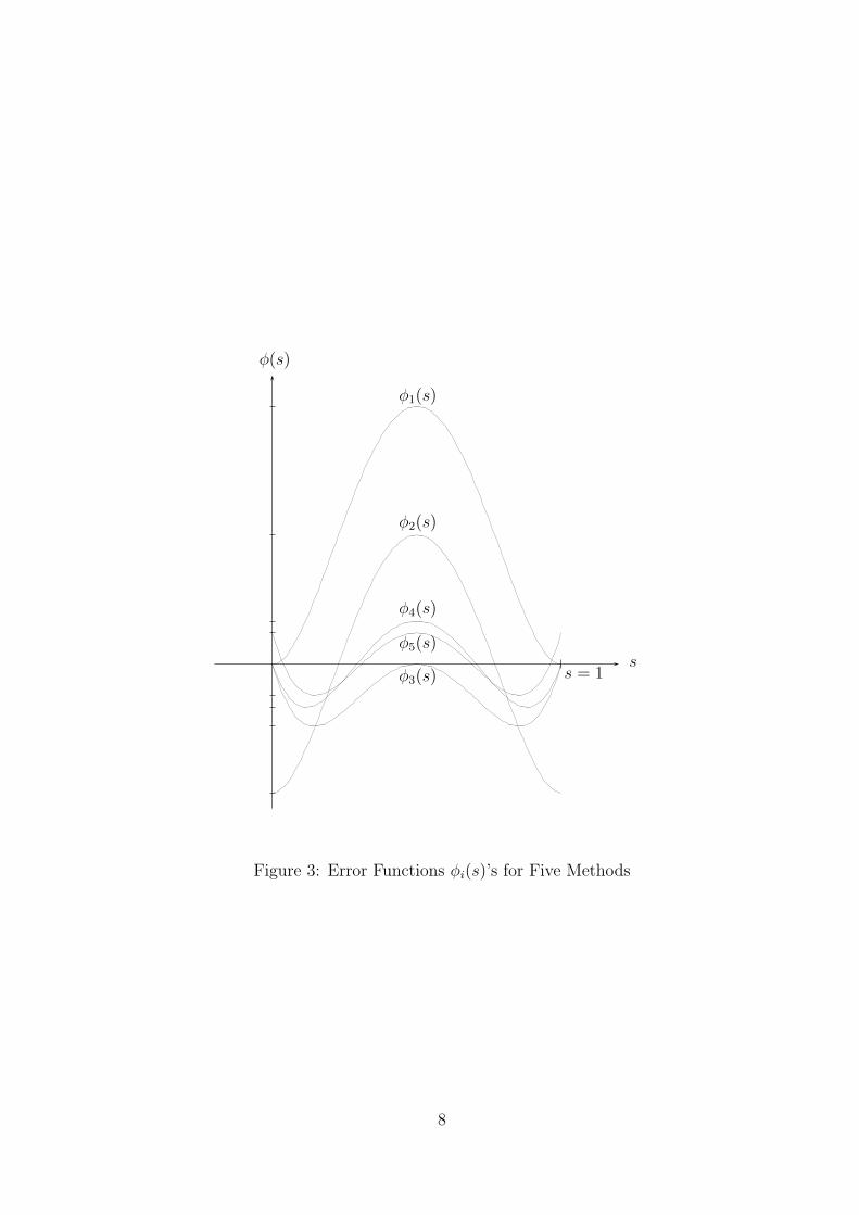
is the first nonzero term in a power series expansion of the error around α = 0. Figure 3

shows the function φ1(s) of this method. The approximation error can be further reduced

by scaling the Bezier control polygons or eliminating the condition of G1-continuity as will

be discussed in the later subsections.

2.3 Method 2: Uniform Scaling of Method 1

The curve Q1(s) of Method 1 lies in the exterior of the unit circle. This means that the

error function φ1(s) takes only nonnegative values. A slightly better approximation can be

obtained by scaling all the three control points simultaneously by a certain magnitude. That

is, the curve Q2(s) = (x2(s), y2(s)), 0 ≤ s ≤ 1, is defined by:

x2(s) = ρx1(s) and y2(s) = ρy1(s), for some ρ > 0.

Then, the error function φ2(s) of this method is given by:

φ2(s) = x22(s) + y

22(s)− 1 = ρ2(x2

1(s) + y21(s))− 1 = ρ2φ1(s) + ρ

2 − 1.

7

φ1(s)

φ2(s)

φ4(s)

φ5(s)

φ3(s)s

φ(s)

s = 1

Figure 3: Error Functions φi(s)’s for Five Methods

8

Multiplying x1(s) and y1(s) by ρ has the same effect as multiplying each control point of

Q1(s) by ρ. Since φ′2(s) = ρ2φ′1(s), the two functions φ1(s) and φ2(s) have their extreme

values at the same parameter values of s. Furthermore, the extremal value δ2(α) = φ2(12)

satisfies:

δ2(α) = ρ2δ1(α) + ρ

2 − 1.

Since φ1(0) = φ1(1) = 0, we have φ2(0) = φ2(1) = ρ2−1. We can minimize the approximation

error by taking ρ so that

φ2(0) + φ2

(1

2

)= 0,

or equivalently,

ρ2 − 1 + ρ2δ1(α) + ρ2 − 1 = 0.

Thus, the value of ρ is given by:

ρ =

√2

2 + δ1(α)=

√√√√ 8 cos2 α2

8 cos2 α2+ sin4 α

2

,

and the approximation error is given by the value:

δ2(α) =δ1(α)

2 + δ1(α)≈ 1

2δ1(α) =

1

128α4 + o(α6),

which means that the size of δ2(α) is slightly less than half of δ1(α). Figure 3 shows the

function φ2(s) of this method.

In order for two consecutive quadratic Bezier curve segments of Method 2 to meet with

G0-continuity, they should have the same angle α. (Note that G1-continuity is also guaran-

teed when the same angle α is used.) This is because the value of ρ depends on the value of

δ1(α), and thus on α, too.

2.4 Method 3: Interpolating Three Circle Points

When the quadratic Bezier curve is not restricted to be tangent to the unit circle at the

two end points of the curve, the approximation error can be further reduced by moving

the middle control point P1 of Method 1 toward the origin along the diagonal line. A

simple approximation is obtained by making the midpoint of the quadratic Bezier curve

Q3(s) = (x3(s), y3(s)) pass through the midpoint of the circular arc; that is, we make

Q3

(12

)= (cos α

2, sin α

2) and φ3

(12

)= 0. The resulting curve Q3(s), 0 ≤ s ≤ 1, always lies

in the interior of the circle. From the condition φ3

(12

)= 0, it follows that D3 = 2 − cos α

2.

Figure 3 shows the function φ3(s) of this method. Maximum errors are obtained at s = s1

and s3 with (negative) magnitude:

δ3(α) = φ3(s1) = φ3(s3) = −1

4

(1− cos

α

2

)2

= − sin4 α

4= − 1

256α4 + o(α6).

9

2.5 Method 4: Interpolation with Equi-oscillating Error

To further reduce the maximum error, the curve can be modified to have an equi-oscillating

error. The error function φ4(s) has the same magnitude of maximum and minimum values

(see Figure 3). ¿From the following polynomial equation of degree four:

φ4(s1) + φ4

(1

2

)= 0,

the corresponding value of D4 can be computed as

D4 = −√2 cos

α

2+

√2 + 2

√2 + cos2

α

2.

Figure 3 shows the function φ4(s) of this method. Maximum errors are obtained at s = s1, s2,

and s3 with magnitude:

δ4(α) = φ4(1

2) =

1

4

[(1−

√2) cos

α

2+

√2 + 2

√2 + cos2

α

2

]2

− 1 = 0.00268α4 + o(α6).

2.6 Method 5: Uniform Scaling of Method 3

The curve Q3(s) of Method 3 is contained in the interior of the unit circle. This means that

the error function φ3(s) takes only nonpositive values. By using a similar scaling technique

to Method 2, a better approximation can be obtained. Let the curve Q5(s) be defined by:

Q5(s) = (x5(s), y5(s)) = (ρx3(s), ρy3(s)), for 0 ≤ s ≤ 1,

where

ρ =

√2

2 + δ3(α)=

√√√√ 2

2− sin4 α4

.

(Note that δ3(α) < 0 and ρ > 1.) Then the approximation error is given as:

δ5(α) =δ3(α)

2 + δ3(α)≈ 1

2δ3(α) = − 1

512α4 + o(α6).

Since δ3(α) < 0, the absolute value |δ5(α)| is slightly larger than half of |δ3(α)|. Figure 3

shows the function φ5(s) of this method. For two adjacent quadratic Bezier curve segments

of Method 5 to meet with G0-continuity, they should have the same angle α.

The actual absolute maximum error values of εi(α), i = 1, . . . , 5, for the five methods are

given by:

εi(α) = max0≤s≤1

|εi(s)| = |√δi(α) + 1− 1|.

The maximum error occurs at s2 =12in Method 1, at s1 and s3 in Method 3, at s1, s2 =

12,

s3 in Methods 2, 4, and at s0, s1, s2, s3, and s4 in Method 5. Table 1 and Figure 4 show the

maximum errors εi(α), i = 1, . . . , 5, of the five methods with respect to various values of α.

The error ε5 is about half of ε3, ε2 is about half of ε1, and ε4 is about 0.7ε3.

10

α (degree) ε1 ε2 ε3 ε4 ε5

90.0 6.07 × 10−2 2.90 × 10−2 1.07 × 10−2 7.72 × 10−3 5.29 × 10−3

70.0 2.00 × 10−2 9.83 × 10−3 4.08 × 10−3 2.89 × 10−3 2.03 × 10−3

50.0 4.84 × 10−3 2.41 × 10−3 1.10 × 10−3 7.65 × 10−4 5.48 × 10−4

30.0 6.01 × 10−4 3.00 × 10−4 1.45 × 10−4 1.00 × 10−4 7.26 × 10−5

10.0 7.27 × 10−6 3.63 × 10−6 1.81 × 10−6 1.24 × 10−6 9.05 × 10−7

5.0 4.53 × 10−7 2.27 × 10−7 1.13 × 10−7 7.77 × 10−8 5.66 × 10−8

1.0 7.25 × 10−10 3.62 × 10−10 1.81 × 10−10 1.24 × 10−10 9.06 × 10−11

Table 1: The Values of εi(α) for Five Methods.

0

10

20

30

40

50

60

70

80

90

1e-11 1e-10 1e-09 1e-08 1e-07 1e-06 1e-05 0.0001 0.001 0.01 0.1

Method 1Method 2Method 3Method 4Method 5

α (degree)

ε

Figure 4: The Inverse Functions of εi(α)’s

11

3 Approximating Planar Offset Curves

In this section, we consider a regular parametric polynomial/rational curve C(t) of degree d

and its offset approximation with piecewise rational curves. The approximation is based on

the hodographs of the curve C(t) and the quadratic Bezier curve segments, Q(s)’s, which

approximate the unit circle. We assume the parametric curve C(t) is C1-continuous.

3.1 Hodograph of a Planar Curve

The hodograph H(t) of a C1-continuous parametric curve C(t) is the locus of the first

derivative C ′(t). For example, the hodograph of a quadratic curve is a straight line and a

cubic curve has a quadratic hodograph curve. We summarize below some properties of the

hodograph which will be used for the approximation of offset curves.

Definition 3.1 Let C(t) = (x(t), y(t)), t1 ≤ t ≤ t2, be a planar regular parametric curve.

The mapping θC,

θC : t ∈ [t1, t2] �→ θC(t) = arctany′(t)x′(t)

∈ [0, 2π),

is called the tangential angular map of the curve C(t).

Lemma 3.1 Let HQ(s) = (x′Q(s), y′Q(s)) be the hodograph of Q(s) = (xQ(s), yQ(s)), s1 ≤

s ≤ s2. If the tangential angular map θQ(s) of Q(s) is one-to-one, any ray L (starting fromthe origin) intersects with HQ(s) at no more than one point.

Proof: Suppose L intersects with HQ(s) at two different points HQ(sa) and HQ(sb), s1 ≤sa < sb ≤ s2. Then, Q′(sa) = (x′Q(sa), y

′Q(sa)) and Q

′(sb) = (x′Q(sb), y′Q(sb)) have the same

direction, which implies that θQ(sa) = θQ(sb). This is a contradiction to the fact that θQ is

one-to-one. ��

Lemma 3.2 Let HQ(s) = (x′Q(s), y′Q(s)) and H(t) = (x′(t), y′(t)) be the hodographs of

Q(s) = (xQ(s), yQ(s)), s1 ≤ s ≤ s2, and C(t) = (x(t), y(t)), t1 ≤ t ≤ t2, respectively.

Furthermore, let HQ(s0) and H(t0) be the intersection points of a ray L (starting from the

origin) with HQ(s) and H(t), respectively. Then, Q(s) and C(t) have the same tangent

direction at Q(s0) and C(t0), respectively.

Proof: The direction of L is the same asHQ(s0) = (x′Q(s0), y′Q(s0)) andH(t0) = (x′(t0), y′(t0)).

Therefore, Q′(s0) = (x′Q(s0), y′Q(s0)) and C

′(t0) = (x′(t0), y′(t0)) have the same direction. ��

12

3.2 Approximated Offset Curve

Assume the tangential angular map θQ is one-to-one and θC([t1, t2]) ⊂ θQ([s1, s2]). For eacht ∈ [t1, t2], consider the ray Lt which starts from the origin and passes through H(t). By

Lemma 3.1, the ray Lt intersects with the hodograph curve HQ at a unique point HQ(s(t)),

where s(t) ∈ [s1, s2]. This means that the mapping, t ∈ [t1, t2] �→ s(t) ∈ [s1, s2], is well-

defined. By Lemma 3.2, Q′(s(t)) and C ′(t) have the same direction. Therefore, the convo-

lution curve C(t) +Q(s(t)) is also well-defined for t ∈ [t1, t2].

A quadratic curve Q(s), s1 ≤ s ≤ s2, has a linear one-to-one hodograph curve HQ(s) =

(as+b, cs+d), where a, b, c, d ∈ R. If Q′(s(t)) = (as(t)+b, cs(t)+d) and C ′(t) = (x′(t), y′(t))

have the same direction, we have:

cs(t) + d

as(t) + b=y′(t)x′(t)

,

and the parameter s(t) ∈ [s1, s2] is uniquely determined by:

s(t) =by′(t)− dx′(t)cx′(t)− ay′(t) . (1)

The approximated offset curve Car (t), t1 ≤ t ≤ t2, is defined by:

Car (t) = C(t) + r ·Q(s(t)),

where s(t) is given in Equation (1). The curve Car (t) is the envelope curve of Q(s) along

the parametric trajectory curve C(t) [2]. For a polynomial curve C(t) of degree d, the

reparametrized curve Q(t) = Q(s(t)) is a planar rational curve of degree 2(d− 1). Thus, the

approximated offset curve, Car (t) = C(t) + r · Q(s(t)), is a planar rational curve of degree

3d − 2. For a rational polynomial curve C(t) of degree d, the function s(t) is a rational

polynomial of degree 2d− 2. Therefore, Q(s(t)) is a rational curve of degree 2(2d− 2), and

Car (t) is a rational curve of degree 5d− 4.

When the curve C(t) is a non-trimmed (infinite or closed) curve and there is no self-

intersection in the exact and approximated offset curves, the global error between Cr(t)

and Car (t) is bounded by r · ε, where ε is the maximum error between the unit circle and

the quadratic Bezier curve approximations, Q(s)’s. In this special case, the sweeping of the

circular disk of radius r generates a connected banded region (in the plane) which is bounded

by two disjoint boundary curves. The exact offset curve Cr(t) is one of the two boundary

curves. Similarly, the approximated offset curve Car (t) is a boundary curve of the sweeping

volume of a convex region (bounded by the quadratic Bezier curve segments, r · Q(s)’s).Since this convex region is in between the two offset circles of radii r(1 − ε) and r(1 + ε),the boundary curve Ca

r (t) is also in between the two offset boundary curves Cr(1−ε)(t) and

13

x

y

Q

S1 : x2 + y2 = r2

C(t) = (t, |t|)

Cr(t)

Car (t)

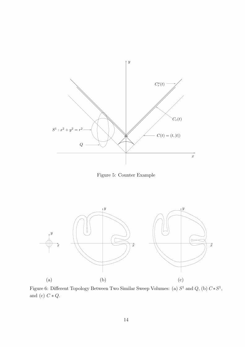
Figure 5: Counter Example

x

y

x

y

x

y

(a) (b) (c)

Figure 6: Different Topology Between Two Similar Sweep Volumes: (a) S1 and Q, (b) C ∗S1,

and (c) C ∗Q.

14

Cr(1+ε)(t), both of which are at distance r · ε from the exact offset curve Cr(t). Therefore,

the distance between Car (t) and Cr(t) is also bounded by r · ε.

Remark: When the curve C(t) is a trimmed curve segment or there is self-intersection in the

exact/approximated offset curve, the global error between Cr(t) and Car (t) is not guaranteed

to be bounded by r · ε. One of the referees of this paper pointed out this fact with the

counter-example shown in Figure 5. The distance between Cr(t) and Car (t) is more than r · ε

near the curve ends and the self-intersections.

The boundary of a 2D curved object is usually modeled with a finite sequence of trimmed

parametric curve segments. Two consecutive curve segments may share a common vertex at

which they haveG1-discontinuity. To eliminate this limitation of trimmed curve segments, we

may treat each vertex as a circular arc of radius 0 which smoothly connects two consecutive

curve segments with C1-continuity. In this way, the object boundary may be considered as

a single C1-continuous closed curve.

More serious is the limitation resulting from the self-intersections of offset curves. In

Figure 5, the distance between Cr(t) and Car (t) (in the middle portions of the two curves) can

be bounded by r ·ε after the self-intersections are eliminated. However, this special treatment

may not work out in general. By sweeping an approximated convex object (instead of the

exact offset disk), the approximated sweep volume may have a different topology from the

exact sweep volume (see Figure 6). In practice, the error bound r · ε is usually taken to

be a very small quantity. The topological changes in the sweep volumes are realized only

when the sweep boundaries have almost tangential intersections within the distance 2r · ε.Therefore, this kind of degeneracy is predictable.

The tangential intersections among offset curve segments introduce various difficulties

in the determination of offset curve arrangement. In the current implementation, we first

determine the topology of the offset boundary by using a polygonal approximation, and

then compute the offset boundary curve approximation within an r · ε bound using the

rational curve segments, Car (t)’s. Therefore, the issue resulting from self-intersecting offset

curves is intentionally eliminated. (See Section 4 for more details and the justification of

this approach.)

3.3 Subdivision of the Curve C(t)

The input curve C(t), t1 ≤ t ≤ t2, is subdivided into finer curve subsegments, Ci(t)’s, so that

each subsegment Ci(t), ti1 ≤ t ≤ ti2 , satisfies the condition: θCi([ti1 , ti2 ]) ⊂ θQj

([sj1 , sj2 ]) for

some quadratic Bezier curve segmentQj(s), sj1 ≤ s ≤ sj2 . (The notationQj’s here means the

consecutive quadratic curve segments in the circle approximation. This is different from the

15

Method 1 Method 2 Method 3 Method 4 Method 5

x

y

x

y

x

y

x

y

x

y

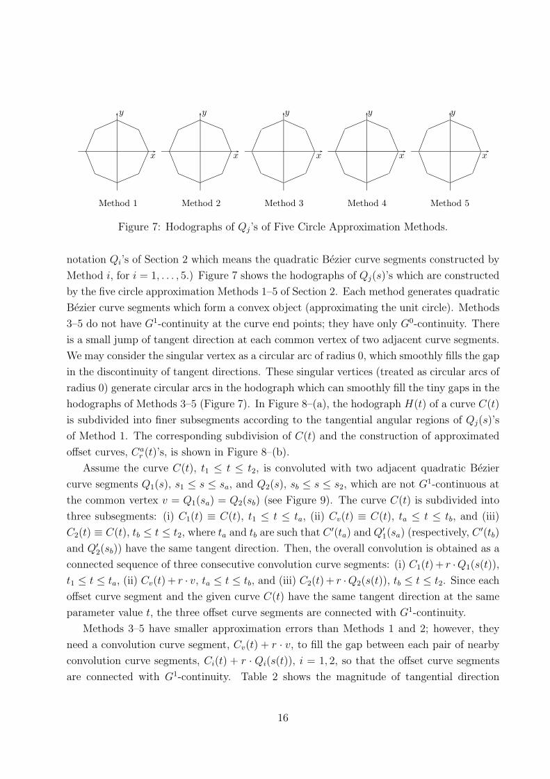
Figure 7: Hodographs of Qj’s of Five Circle Approximation Methods.

notation Qi’s of Section 2 which means the quadratic Bezier curve segments constructed by

Method i, for i = 1, . . . , 5.) Figure 7 shows the hodographs of Qj(s)’s which are constructed

by the five circle approximation Methods 1–5 of Section 2. Each method generates quadratic

Bezier curve segments which form a convex object (approximating the unit circle). Methods

3–5 do not have G1-continuity at the curve end points; they have only G0-continuity. There

is a small jump of tangent direction at each common vertex of two adjacent curve segments.

We may consider the singular vertex as a circular arc of radius 0, which smoothly fills the gap

in the discontinuity of tangent directions. These singular vertices (treated as circular arcs of

radius 0) generate circular arcs in the hodograph which can smoothly fill the tiny gaps in the

hodographs of Methods 3–5 (Figure 7). In Figure 8–(a), the hodograph H(t) of a curve C(t)

is subdivided into finer subsegments according to the tangential angular regions of Qj(s)’s

of Method 1. The corresponding subdivision of C(t) and the construction of approximated

offset curves, Car (t)’s, is shown in Figure 8–(b).

Assume the curve C(t), t1 ≤ t ≤ t2, is convoluted with two adjacent quadratic Bezier

curve segments Q1(s), s1 ≤ s ≤ sa, and Q2(s), sb ≤ s ≤ s2, which are not G1-continuous at

the common vertex v = Q1(sa) = Q2(sb) (see Figure 9). The curve C(t) is subdivided into

three subsegments: (i) C1(t) ≡ C(t), t1 ≤ t ≤ ta, (ii) Cv(t) ≡ C(t), ta ≤ t ≤ tb, and (iii)

C2(t) ≡ C(t), tb ≤ t ≤ t2, where ta and tb are such that C ′(ta) and Q′1(sa) (respectively, C

′(tb)

and Q′2(sb)) have the same tangent direction. Then, the overall convolution is obtained as a

connected sequence of three consecutive convolution curve segments: (i) C1(t)+ r ·Q1(s(t)),

t1 ≤ t ≤ ta, (ii) Cv(t) + r · v, ta ≤ t ≤ tb, and (iii) C2(t) + r ·Q2(s(t)), tb ≤ t ≤ t2. Since eachoffset curve segment and the given curve C(t) have the same tangent direction at the same

parameter value t, the three offset curve segments are connected with G1-continuity.

Methods 3–5 have smaller approximation errors than Methods 1 and 2; however, they

need a convolution curve segment, Cv(t) + r · v, to fill the gap between each pair of nearby

convolution curve segments, Ci(t) + r · Qi(s(t)), i = 1, 2, so that the offset curve segments

are connected with G1-continuity. Table 2 shows the magnitude of tangential direction

16

(a) (b)

Figure 8: (a) Subdivision of H(t), and (b) Corresponding Subdivision of C(t) and Construc-

tion of Car (t).

v

Q1(s)

Q2(s)

∆θ

C1(t)

C2(t)

Cv(t)

C1(t) + r · Q1(s(t))

C2(t) + r · Q2(s(t))

Cv(t) + r · v

y

x

Figure 9: Convolution Curve from Methods 3, 4, and 5

17

α (degree) Method 3, 5 Method 4

90 1.8 × 10−1 1.6 × 10−1

70 9.6 × 10−2 8.2 × 10−2

50 3.7 × 10−2 3.1 × 10−2

30 8.6 × 10−3 7.2 × 10−3

10 3.3 × 10−4 2.7 × 10−4

Table 2: Magnitude of Normal Angle Discontinuity ∆θ (radian)

discontinuity in Methods 3–5. The tangential gap filling curve segment, Cv(t) + r · v, is asimple translation of Cv(t) by a vector r · v; therefore, they have the same size. The length

of the curve segment Cv(t) is between ∆θ/κ1 and ∆θ/κ2, where κ1 and κ2 are the maximum

and minimum curvatures of Cv(t), respectively.

The size of the curve segment, Cv(t) + r · v, is usually larger than the offset curve

approximation error, r · ε, especially when the curve Cv(t) has low curvature (see Tables

1 and 2). When we use Methods 3 and 4, the quadratic Bezier curve Q(s), 0 ≤ s ≤ 1,

has its circle approximation error less than ε on a domain slightly larger than [0, 1]; that

is, |φ(s)| < ε, −∆s ≤ s ≤ 1 + ∆s, for some ∆s > 0 (see Figure 3). Therefore, the two

approximated offset curve segments Ci(t) + r ·Qi(s(t)), i = 1, 2, can be extended into larger

curve segments while staying within the approximation error bound, r ·ε. If the two extendedoffset curve segments intersect, we can remove the gap filling curve segment, Cv(t) + r · v,by filling the gap with the extensions of the two offset curve segments up to their common

intersection point. Otherwise, we can replace the curve segment, Cv(t) + r · v, by the line

segment connecting the two curve end points (if the line approximation has error less than

r · ε). However, in this case, they have only G0-continuity at the intersection point. For G1-

continuity or for the case in which the line approximation has error larger than the tolerance

r · ε, we can use a quadratic Bezier curve approximation of the curve segment, Cv(t) + r · v,if the curve approximation error is less than r · ε.

3.4 Under and Over Estimations

It is sometimes desirable to have an offset approximation which completely overestimates.

In this case, the offset approximation is never below the exact offset distance, only above

or equal to it. Method 1 (respectively, Method 3) completely overestimates (respectively,

underestimates) the exact offset. Clearly, for machining purposes, when the center of the

ball end tool follows the offset approximation, a completely overestimating offset approxi-

18

mation scheme will prevent gauging. This important question has been ignored in the offset

approximation research.

In fact, the method of Cobb [3] completely underestimates the exact offset. In Cobb

[3], an approximated offset curve is computed by translating each control point of the curve

along the normal direction of C(t) at the corresponding node parameter value by a distance

r, and the approximated offset curve Car (t) of a Bezier or B-spline curve C(t) is given by:

Car (t) =

n∑i=0

(Pi + r ·Ni)Bi(t) =n∑

i=0

PiBi(t) + r ·n∑

i=0

NiBi(t) = C(t) + r · V (t),

where Bi(t) is the Bezier or B-spline basis function and Ni is the unit normal vector at

the node parameter value of the corresponding control point Pi of C(t), for each i. Each

control point Ni of the vector field curve V (t) is on the unit circle S1. Hence, by the convex

hull property of the Bezier and B-spline representations, V (t) is contained in the unit ball.

Consequently, we have

‖Car (t)− C(t)‖ = ‖r · V (t)‖ = ‖r ·

n∑i=0

NiBi(t)‖ = r · ‖n∑

i=0

NiBi(t)‖ ≤ r,

which implies that the resulting offset approximation always underestimates the exact offset.

(See [7] for more details.)

Interpolatory schemes [19, 23] are, in general, piecewise overestimating and underesti-

mating the exact offset. Here, if desired, we can alleviate the errors of Methods 1 and

3, making them piecewise overestimating and underestimating using scaling as is done in

Methods 2 and 5. The piecewise overestimating and underestimating offset approximation

may be sufficient when the offset is employed as a modeling tool, for instance. Hence, mak-

ing the offset approximation more accurate (at the expense of sacrificing the overestimation

property) might be profitable in this instance.

4 Eliminating Self-Intersecting Loops

In this section, we consider how to compute the offset of a planar curved object. The offsets

of boundary curves are first computed; then, their local and global self-intersections are elim-

inated. Examples of local and global loops are shown in Figure 10–(c). The determination

of self-intersecting loops is closely related with the arrangement of offset curve segments [13].

A robust implementation of curve arrangement is one of the most difficult open problems in

geometric modeling [14]. The only reliable robust implementation today is to use polygonal

approximations of the offset curve segments and determine the arrangement of resulting line

segments. (See Reference [12] for the current state-of-the-art of robust line segments ar-

rangement in the plane.) Ahn, Kim, and Lim [1] demonstrated the efficiency and robustness

19

(a) (b) (c)

(d) (e) (f)

(g) (h) (i)

Global Loop

Local Loops

Figure 10: Elimination of Self-Intersection Loops

20

of this technique in approximating the boundary of a 2D general sweep. The general sweep

is the most general form of sweep in which the moving object changes its shape dynamically

while moving along a trajectory curve. The offset computation is a special case of general

sweep computation. Therefore, the general technique of Reference [1] can be applied to the

case of offsetting. There are also some computational shortcuts to be applied in the special

case of offsetting [20].

The input curve is approximated by discrete points and their connecting piecewise line

segments (Figure 10–(b)). The offset curve is then approximated by the offsets of the dis-

crete points (Figure 10–(c)). (Lee and Kim [20] have more details on how to approximate

the offset computation error in this discrete approximation method for planar curves.) The

offset polygon may have redundancies which do not contribute to the final offset boundary.

For example, the segment between each pair of corresponding cusps in the offset polygon

is redundant since the segment belongs to the interior of the offset object. Each cusp cor-

responds to the curve point which has curvature equal to 1/r, where r is the offset radius.

The input curve subsegment which has curvature higher than 1/r should be eliminated from

consideration. Let a line segment )p = p1p2 be offset into a line segment )o = o1o2. We can

easily observe that, in a local redundant segment, the inner product of two vectors, )p · )o,has negative value [6]. Figure 10–(d) shows the offset polygon after eliminating these lo-

cal redundant offset segments. In the next step, we use a plane sweep algorithm to detect

all the intersections among the offset line segments (Figure 10–(e)), and construct a valid

boundary topology for the offset polygon (Figure 10–(f)). Ahn, Kim, and Lim [1] suggested

an efficient and robust plane sweep algorithm which constructs the boundary of a polygonal

approximation of the general sweep. We use a similar algorithm in this paper.

Once we have computed a polygonal approximation of the offset boundary, we can easily

extract the valid parameter intervals of the boundary curve of the input object. These

valid intervals correspond to the object boundary segments which contribute to the offset

boundary segments (Figure 10–(g)). However, a direct computation of approximated offset

curve segments from these valid parameter intervals may not lead to a correct result. The

intersection points of polygonal approximations may not provide accurate parameter values

for the intersection points of the offset curve segments. We need to refine the numerical

precision of the intersection points among offset curve segments [16]. For this purpose, the

intersections among offset line segments are used as initial solutions (Figure 10–(e)). In

Figure 10–(h), the offset curve end points are refined from the small segments shown in thick

curves. Figure 10–(i) shows the final offset boundary and the original input object boundary.

The polygonal approximation may omit some valid loops in the offset. A simple way to

resolve this problem might be to approximate the input curve with high precision. How-

ever, this method generates many tiny line segments which cause problems in robustness

21

as well as computational efficiency. The missing loops are due to the tangential and/or

multiple intersections of the offset curve segments. These degeneracies correspond to the

topological changes of the offset boundary as the offset radius r is slightly changed. For each

degeneracy, the corresponding offset curve segments are intersected with high precision to

determine a correct topology. However, it is not always possible to determine the correct

topological arrangement while making them consistent with the numerical curve intersection

data, especially when the curve segments have (almost) tangential/multiple intersections

[15].

5 Experimental Results

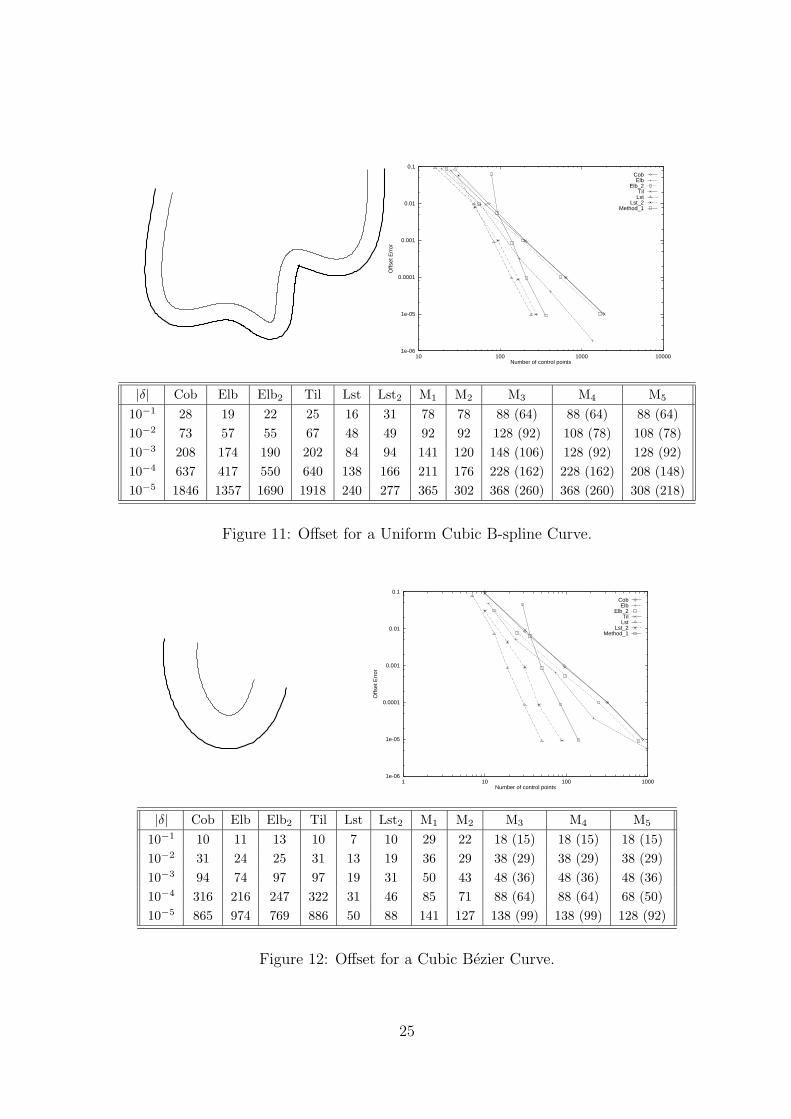
Figures 11–13 show some experimental results on the construction of approximated offset

curves. The input curve of Figure 11 is a uniform cubic B-spline curve with 7 control points:

(−3.01619, 2.34143), (−3.97193, −2.20842), (−1.07045, 0.0722807), (0.319568, −2.77522),(−0.152767, 2.299), (2.92416, −0.939865), and (2.8027, 3.02775). An offset radius 0.5 is usedfor the example. For each tolerance |δ|, approximated offset curves of (rational) degree 7 are

generated by using the convolution with the quadratic Bezier curve segments of Methods

1–5. They are compared with the offset curves generated by other methods, in terms of the

number of control points generated.

The input curve for Figure 12 is a cubic Bezier curve with 4 control points: (−0.785938,0.891849), (−0.993306, −0.59695), (0.3, −2.5), and (0.9, −0.2). An offset radius 1.0 is used

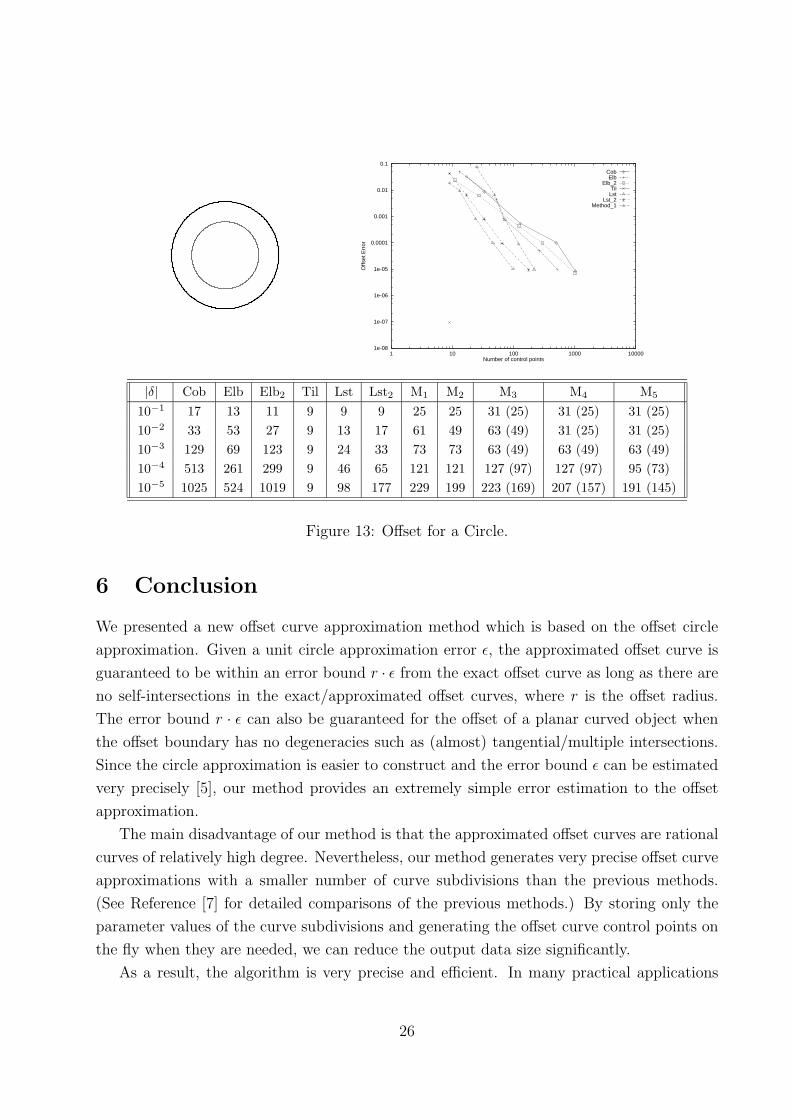
and approximated offset curves of (rational) degree 7 are generated. In Figure 13, the input

circle is represented by a rational quadratic B-spline curve with 4 curve segments and a total

of 9 control points. An offset radius 0.6 is used and approximated offset curves of (rational)

degree 6 are generated. Note that, in Methods 3–5, the convolution curve segments, Cv(t)+v,

have the same degree as the base curve since they are simple translations of the original curve

subsegments.

The table in each figure shows the numbers of control points for the approximated offset

curves generated by different methods. The columns under labels M1, . . . ,M5 provide the

results of Methods 1,. . . ,5, respectively. In Methods 3–5, the convolution curve segments,

Cv(t) + v, may be further approximated by points, line segments, and quadratic curve seg-

ments within the given error bound (see the discussion at the end of Section 3.3). The

numbers in parentheses (of Methods 3–5) show the best case lower bounds in which all the

convolution curve segments, Cv(t)+v, could be replaced by points. The tolerances are given

by the value of |δ|, which is the absolute maximum value of the function: φ(t) ≈ 2ε(t) (see

Section 2.1).

The method Cob corresponds to the divide-and-conquer based method of Cobb [3], in

22

which the global error bounding method of [6] is adapted to measure the offset approximation

error instead of measuring the distance between the midpoints of the exact and approximated

offset curves. If the approximation error is above the given tolerance, the input curve is

subdivided at the midpoint of the curve. Most of the previous methods belong to this class

of midpoint subdivision. The method Elb corresponds to the adaptive subdivision method

of Elber and Cohen [6] which is applied to the offset curve construction method of Cobb [3].

When the approximation error is above the given tolerance, a knot point is inserted at the

parameter value which corresponds to the maximum error. The method Elb2 is a variation

of Elb which subdivides the input curve at the parameter value of maximum error.

The method Til is an extension of Tiller and Hanson [24] while adapting the global error

bounding technique of [6]. The control polygon of an input spline curve is offset to define the

control polygon of the offset curve. In Figure 13, the input circle is represented by a rational

quadratic B-spline curve for which the control polygon has a regular shape. Therefore, the

offset control polygon also has a regular shape and represents the exact offset circle with

no approximation error. As long as the control polygon of an input curve has no sharp

corner, the method of Tiller and Hanson [24] performs very nicely. However, as shown in

the examples of Figures 11 and 12, when the control polygon has sharp corners, the offset

control polygon does not provide a good approximation to the exact offset curve.

The method Lst is an extension of Hoschek and Wissel [18] while adapting the global

error bounding technique of [6]. Instead of sampling only the midpoint, a finite number of

sample points are generated and the approximated offset curve is constructed as a uniform

B-spline curve. The B-spline control points are determined so that they generate a piecewise

cubic B-spline curve with the least squares error from the discrete sample points. If the

approximation error is above the given tolerance, instead of subdividing the input curve

as in [18], more control points are used for the construction of an approximated offset B-

spline curve. This modification reduces the total number of control points generated. The

method Lst2 is a variation of Lst which subdivides the input curve at the parameter value

of maximum error.

Except for some special cases such as the one shown in Figure 13, the optimization based

method Lst generates a smaller number of control points than all the other methods. Our

method ranks just next to the methods Lst and Lst2 for high precision offset approximation.

The main reason why our method generates more control points than Lst and Lst2 is that

our offset curves have relatively high degree. Because of this, our method performs worse

than all the other methods up to the approximation error 10−2 in the examples shown in Fig-

ures 11–13. However, when we consider the number of curve subdivisions as the performance

criterion, our method performs better. For example, in Figure 11, the number of offset curve

segments generated by Methods 1–2 is about 7 times less than the number of control points,

23

which is even less than the number of cubic B-spline offset curve segments generated by the

method Lst . The question is: what is the rationale to support this performance criterion ?

As one might have realized in the offset examples of Figures 11–13, data explosion is a se-

rious problem in offset computation, especially for high precision approximation. Therefore,

it is necessary to store only a minimum amount of computation results and generate all the

other geometric information from these minimum data on the fly when they are required. In

the case of subdivision based methods [3, 4, 17, 19, 23, 24], we can store only the parameter

values of the base curve at which the curve subdivisions have been made. It is quite straight-

forward to generate the control points of the offset curve segments on the fly from these knot

points on the base curve. Storing the corresponding parameter values instead of the control

points reduces the data storage significantly. In our method, assuming degree 7 rational

curves are used for the offset curve approximation, this storage reduction would result in a

significant saving, with almost 14 times less output data size. Unfortunately, it is difficult

to apply this technique to the optimization based method Lst since the method Lst applies

the B-spline curve approximation directly to the offset curve. Therefore, the relationship

between the control point and the base curve parameter value is not clear. However, for this

purpose, we can use the method Lst2 instead of Lst since the base curve subdivision is used

in Lst2.

Figure 14 shows the result of this storage reduction technique applied to the examples

shown in Figures 11–13. The numbers of base curve subdivisions are shown for the subdi-

vision based methods. The method Lst2 produces a smaller number of curve subdivisions

when higher degree B-spline curve segments are used for the offset curve approximation.

However, we have not used high degree curves in the experiment because of high compu-

tational requirement for the evaluation of global error bounds in the offset approximation,

especially for high precision approximation. This fact also demonstrates the effectiveness

of our methods in that the global error bounds are estimated automatically by measuring

the circle approximation errors. Once the range of curve tangent directions has been com-

puted, given any offset approximation error, the number of required curve subdivisions are

estimated a priori without doing any curve subdivision at all.

Figure 15 shows some practical examples which require this kind of output data size

reduction. The first three examples (a)–(c) have applications in the generation of decorative

fonts and shapes in desktop publishing. The last example (d) has applications in the gen-

eration of NC tool paths for pocket machining. In these applications, the data explosion is

a serious problem. The examples are generated by offsetting 2D curved objects. The base

objects are shown in thick curves and their offsets for various offset radii are shown in thin

curves. They are constructed by eliminating all the self-intersecting loops of the offset curves

(see Section 4). All the input curves are uniform cubic B-spline curves.

24

1e-06

1e-05

0.0001

0.001

0.01

0.1

10 100 1000 10000

Offs

et E

rror

Number of control points

CobElb

Elb_2Til

LstLst_2

Method_1

|δ| Cob Elb Elb2 Til Lst Lst2 M1 M2 M3 M4 M5

10−1 28 19 22 25 16 31 78 78 88 (64) 88 (64) 88 (64)10−2 73 57 55 67 48 49 92 92 128 (92) 108 (78) 108 (78)10−3 208 174 190 202 84 94 141 120 148 (106) 128 (92) 128 (92)10−4 637 417 550 640 138 166 211 176 228 (162) 228 (162) 208 (148)10−5 1846 1357 1690 1918 240 277 365 302 368 (260) 368 (260) 308 (218)

Figure 11: Offset for a Uniform Cubic B-spline Curve.

1e-06

1e-05

0.0001

0.001

0.01

0.1

1 10 100 1000

Offs

et E

rror

Number of control points

CobElb

Elb_2Til

LstLst_2

Method_1

|δ| Cob Elb Elb2 Til Lst Lst2 M1 M2 M3 M4 M5

10−1 10 11 13 10 7 10 29 22 18 (15) 18 (15) 18 (15)10−2 31 24 25 31 13 19 36 29 38 (29) 38 (29) 38 (29)10−3 94 74 97 97 19 31 50 43 48 (36) 48 (36) 48 (36)10−4 316 216 247 322 31 46 85 71 88 (64) 88 (64) 68 (50)10−5 865 974 769 886 50 88 141 127 138 (99) 138 (99) 128 (92)

Figure 12: Offset for a Cubic Bezier Curve.

25

1e-08

1e-07

1e-06

1e-05

0.0001

0.001

0.01

0.1

1 10 100 1000 10000

Offs

et E

rror

Number of control points

CobElb

Elb_2Til

LstLst_2

Method_1

|δ| Cob Elb Elb2 Til Lst Lst2 M1 M2 M3 M4 M5

10−1 17 13 11 9 9 9 25 25 31 (25) 31 (25) 31 (25)10−2 33 53 27 9 13 17 61 49 63 (49) 31 (25) 31 (25)10−3 129 69 123 9 24 33 73 73 63 (49) 63 (49) 63 (49)10−4 513 261 299 9 46 65 121 121 127 (97) 127 (97) 95 (73)10−5 1025 524 1019 9 98 177 229 199 223 (169) 207 (157) 191 (145)

Figure 13: Offset for a Circle.

6 Conclusion

We presented a new offset curve approximation method which is based on the offset circle

approximation. Given a unit circle approximation error ε, the approximated offset curve is

guaranteed to be within an error bound r · ε from the exact offset curve as long as there are

no self-intersections in the exact/approximated offset curves, where r is the offset radius.

The error bound r · ε can also be guaranteed for the offset of a planar curved object when

the offset boundary has no degeneracies such as (almost) tangential/multiple intersections.

Since the circle approximation is easier to construct and the error bound ε can be estimated

very precisely [5], our method provides an extremely simple error estimation to the offset

approximation.

The main disadvantage of our method is that the approximated offset curves are rational

curves of relatively high degree. Nevertheless, our method generates very precise offset curve

approximations with a smaller number of curve subdivisions than the previous methods.

(See Reference [7] for detailed comparisons of the previous methods.) By storing only the

parameter values of the curve subdivisions and generating the offset curve control points on

the fly when they are needed, we can reduce the output data size significantly.

As a result, the algorithm is very precise and efficient. In many practical applications

26

|δ| Cob Elb2 Til Lst2 M1 M2 M3 M4 M5

10−1 7 5 6 8 10 10 8 8 810−2 22 16 20 14 12 12 12 10 1010−3 67 61 65 29 19 16 14 12 1210−4 210 181 211 53 29 24 22 22 2010−5 613 561 637 90 51 42 36 36 30

(a)

|δ| Cob Elb2 Til Lst2 M1 M2 M3 M4 M5

10−1 2 3 2 2 3 2 1 1 110−2 9 7 9 5 4 3 3 3 310−3 30 31 31 9 6 5 4 4 410−4 104 81 106 14 11 9 8 8 610−5 287 255 294 28 19 17 13 13 12

(b)

|δ| Cob Elb2 Til Lst2 M1 M2 M3 M4 M5

10−1 4 1 0 0 0 0 0 0 010−2 12 9 0 4 6 4 4 0 010−3 60 57 0 12 8 8 4 4 410−4 252 145 0 28 16 16 12 12 810−5 508 505 0 84 34 29 24 24 20

(c)

Figure 14: Number of Curve Subdivisions: (a) Figure 11, (b) Figure 12, and (c) Figure 13

27

(a) (b)

(c) (d)

Figure 15: (a) H Shape, (b) Human Shape, (c) Oryx Shape, and (d) Pocket Machining Paths

28

of planar curve offsetting (e.g., NC tool path generation), the accuracy of the offset curve

approximation and the reduction of output data size are more important than any other

criteria.

7 Acknowledgement

The authors thank the anonymous referees for their valuable comments and constructive

suggestions. The counter-example shown in Figure 5 was provided by one of the referees.

References

[1] Ahn, J.-W., Kim, M.-S., and Lim, S.-B., (1993), “Approximate General Sweep Bound-

ary of a 2D Curved Object,” CVGIP: Graphical Models and Image Processing , Vol. 55,

No. 2, pp. 98–128.

[2] Bajaj, C., and Kim, M.-S., (1989), “Generation of Configuration Space Obstacles: The

Case of Moving Algebraic Curves,” Algorithmica, Vol. 4, No. 2, pp. 157–172.

[3] Cobb, B., (1984), Design of Sculptured Surfaces Using The B-spline Representation,

Ph.D. thesis, University of Utah, Computer Science Department.

[4] Coquillart, S., (1987), “Computing Offset of B-spline Curves,” Computer-Aided Design,

Vol. 19, No. 6, pp. 305–309.

[5] Dokken, T., Daehlen, M., Lyche, T., and Morken, K., (1990), “Good Approximation of

Circles by Curvature-Continuous Bezier Curves,” Computer Aided Geometric Design,

Vol. 7, pp. 33–41.

[6] Elber, G., and Cohen, E., (1991), “Error Bounded Variable Distance Offset Operator

for Free Form Curves and Surfaces,” International Journal of Computational Geometry

and Applications , Vol. 1, No. 1, pp. 67–78.

[7] Elber, G., Lee, I.-K., and Kim, M.-S., (1995), “State of the Art in Offset Approximation

of Freeform Curves,” Manuscript, September, 1995.

[8] Farouki, R., and Neff, C., (1990), “Analytic Properties of Plane Offset Curves,” Com-

puter Aided Geometric Design, Vol. 7, pp. 83–99.

[9] Farouki, R., and Neff, C., (1990), “Algebraic Properties of Plane Offset Curves,” Com-

puter Aided Geometric Design, Vol. 7, pp. 101–127.

29

[10] Farouki, R., and Sakkalis, T., (1990), “Pythagorean-hodographs,” IBM Journal of Re-

search and Development , Vol. 34, pp. 736–752.

[11] Goldapp, M., (1991), “Approximation of Circular Arcs by Cubic Polynomials,” Com-

puter Aided Geometric Design, Vol. 8, pp. 227–238.

[12] Guibas, L., and Marimont, D., (1995), “Rounding Arrangements Dynamically,”

Proc. 11th Annual Symp. on Computational Geometry , pp. 190–199.

[13] Guibas, L., Ramshaw, L., and Stolfi, J., (1983), “A Kinetic Framework for Compu-

tational Geometry,” Proc. 24th Annual Symp. on Foundations of Computer Science,

pp. 100–111.

[14] Held, M., (1991), On the Computational Geometry of Pocket Machining , Lecture Notes

in Computer Science, Vol. 500, Springer-Verlag.

[15] Hoffmann, C., (1989), Geometric & Solid Modeling: An Introduction, Morgan Kauf-

mann Pub., San Mateo, California.

[16] Hoschek, J., (1985), “Offset Curves in the Plane,” Computer-Aided Design, Vol. 17,

No. 2, pp. 77–82.

[17] Hoschek, J., (1988), “Spline Approximation of Offset Curves,” Computer Aided Geo-

metric Design, Vol. 5, pp. 33–40.

[18] Hoschek, J., and Wissel, N., (1988), “Optimal Approximate Conversion of Spline Curves

and Spline Approximation of Offset Curves,” Computer-Aided Design, Vol. 20, No. 8,

pp. 475–483.

[19] Klass, R., (1983), “An Offset Spline Approximation for Plane Cubic Splines,” Computer-

Aided Design, Vol. 15, No. 4, pp. 297–299.

[20] Lee, I.-K., and Kim, M.-S., (1992), “Primitive Geometric Operations on Planar Al-

gebraic Curves with Gaussian Approximation,” Visual Computing , T.L. Kunii (Ed.),

Springer-Verlag, 1992, pp. 449–468.

[21] Morken, K., (1991), “Best Approximation of Circle Segments by Quadratic Bezier

Curves,” Curves and Surfaces, P.J. Laurent, A. Le Mehaute, and L.L. Schumaker (Eds.),

Academic Press, Boston, pp. 331–336.

[22] Persson, H., (1978), “NC Machining of Arbitrarily Shaped Pockets,” Computer-Aided

Design, Vol. 10, No. 4, pp. 169–174.

30

[23] Pham, B., (1988), “Offset Approximation of Uniform B-splines,” Computer-Aided De-

sign, Vol. 20, No. 8, pp. 471–474.

[24] Tiller, W., and Hanson, E., (1984), “Offsets of Two Dimensional Profiles,” IEEE Com-

puter Graphics & Application, Vol. 4, pp. 36–46.

31