arX

iv:h

ep-t

h/05

0608

2v2

29

Jul 2

005

Multi-(super)graviton theory

on topologically non-trivial backgrounds

Guido Cognola ∗,a, Emilio Elizalde †,b,c and Sergio Zerbini ‡,a

aDipartimento di Fisica, Universita di Trentoand Istituto Nazionale di Fisica Nucleare,

Gruppo Collegato di Trento, Italia

bConsejo Superior de Investigaciones CientıficasInstituto de Ciencias del Espacio (ICE/CSIC)

Campus UAB, Facultat Ciencies, Torre C5-Parell-2a planta,08193 Bellaterra (Barcelona), Spain

c Institut d’Estudis Espacials de Catalunya (IEEC),Edifici Nexus, Gran Capita 2-4, 08034 Barcelona, Spain

Abstract: It is shown that in some multi-supergraviton models, the contributions to the effective

potential due to a non-trivial topology can be positive, giving rise in this way to a positive

cosmological constant, as demanded by cosmological observations.

1 Introduction

Renewed interest in the study of multi-graviton theories [1] owes, in particular, to the fact thatthese formulations resemble higher-dimensional gravities in the presence of discrete dimensions.These classes of discretized Kaluza-Klein theories are now in fact under the focus of attentiondue to their primary importance for the realization of the dimensional deconstruction program[2, 3]. Moreover, multigravitons can be also related with discretized brane-world models [4].

In spite of the absence of a consistent interaction among the gravitons, one can think ofpossible couplings in the theory space. In particular, in a recent paper [5], a multi-gravitontheory with nearest-neighbor couplings in the theory space has been proposed. As a result, adiscrete mass spectrum appears. The theory seems to be equivalent to Kaluza-Klein gravitywith a discretized dimension.

In a previous paper concerning multi-graviton theory [6], we have shown by means of anexplicit example, namely a discretized Randall-Sundrum (RS) brane-world [7], that the inducedcosmological constant becomes positive provided the number of massive gravitons is sufficientlylarge.

In the present paper, we would like to show that an alternative mechanisms can also give riseto positive contributions to the cosmological constant. In particular we shall consider a multi-supergraviton example with few gravitons, in a manifold (bulk) with non trivial topology. Weshall show that in such a model a positive cosmological constant Λ can be generated, due to thepresence of positive topological contributions. Moreover, by a suitable choice of the topologicalparameters, the number obtained for Λ can reach a value perfectly in accordance with resultobtained from recent cosmological observations [8].

∗e-mail: cognola@science.unitn.it†e-mail: elizalde@ieec.uab.es‡e-mail: zerbini@science.unitn.it

1

2 The multi-graviton and multi-supergraviton models

2.1 The graviton model

We start by considering the Lagrangian for the spin-two field hµν with mass m

Lm = L0 −m2

2

(

hµνhµν − h2)

− 2 (mAµ + ∂µϕ) (∂νhµν − ∂µh)

−1

2(∂µAν − ∂νAµ) (∂µAν − ∂νAµ) , (2.1)

where L0 is the Lagrangian of the massless spin-two field (graviton) hµν (h ≡ hµµ)

L0 = −1

2∂λhµν∂λhµν + ∂λhλ

µ∂νhµν − ∂µhµν∂νh +

1

2∂λh∂λh , (2.2)

while Aµ and ϕ are Stuckelberg fields [9].The multi-graviton model is defined by taking N−copies of (2.1) with graviton hnµν and

Stuckelberg fields Anµ and ϕn. Here, we propose a theory defined by a Lagrangian which istaken to be a generalization of the one in [5]. It reads

L =N−1∑

n=0

[

−1

2∂λhnµν∂

λhµνn + ∂λhλ

nµ∂νhµνn − ∂µhµν

n ∂νhn +1

2∂λhn∂λhn

−1

2

(

m2∆hnµν∆hµνn − (∆hn)2

)

− 2(

m∆†Aµn + ∂µϕn

)

(∂νhnµν − ∂µhn)

−1

2(∂µAnν − ∂νAnµ) (∂µAν

n − ∂νAµn)

]

. (2.3)

The ∆ and ∆† are difference operators, which operate on the indices n as

∆φn ≡N−1∑

k=0

akφn+k , ∆†φn ≡N−1∑

k=0

akφn−k ,N−1∑

k=0

ak = 0 , (2.4)

where the ak are N constants and the N variables φn can be identified with periodic fields ona lattice with N sites if the periodic boundary conditions φn+N = φn are imposed. The lattercondition in (2.4) assures that ∆ becomes the usual differentiation operator in a properly definedcontinuum limit.

The eigenvalues and eigenvectors for ∆ are given by4

∆φpn = iµpφ

pn , iµp =

N−1∑

n=0

an e2πinp/N , (2.5)

φpn =

e2πinp/N

√N

. p = 0, 1, 2, 3, . . . (2.6)

By using (2.4) in the latter equation and assuming an to be real one gets the relations

µ0 = 0 , µp = −µN−p , µN−p = −µ∗p , (2.7)

4Please note that here we use a different notation with respect to one used in Refs. [6] and [11]. In fact, inorder to avoid confusion with masses, we have replaced the eigenvalue m with µ and the index M with p.

2

which, for any fixed N , permit to obtain the whole spectrum of the theory.Then we see that the Lagrangian (2.3) describes a massless graviton and N − 1 massive

gravitons, with masses Mp = |µp| (p = 1, 2, . . . , N − 1). It must be pointed out that the massivegravitons always appear in pairs which share a common mass and, moreover, the complex massparameter µp can be arbitrarily chosen, just by properly selecting the coefficients ak in (2.5) [6].As discussed in [5], the multigraviton model can be regarded as corresponding to a Kaluza-Kleintheory where the extra dimension lives in a lattice.

As a specific example, we now consider the two-brane Randall-Sundrum (RS) model [7] (fora recent review see [10]). In this model, the masses of the Kaluza-Klein modes are given by

Mp =πp

zc, zc = l

(

eπrc/l − 1)

, p = 0, 1, 2, ... (2.8)

where l is the length parameter of the five-dimensional AdS space and πrc the geodesic distancebetween the two branes.

Motivated by this last equation (2.8), we consider an N = 2N ′ + 1 graviton model, with thegraviton masses being given by

µp =

{ πpzc

, p = 0, 1, · · · , N ′,

−π(N−p)zc

, p = N ′ + 1, N ′ + 2, · · · , N − 1 = 2N ′.

Those are solutions of Eq. (2.5), with the choice a0 = 0 and, for any n ≥ 1,

an = − 2π

(2N ′ + 1)zcIm

(

1 − e−i 2πN

′n

2N′+1

)

e−i 2πn

2N′+1

1 − e−i 2πn

2N′+1

= −(−1)n 2π

Nzc

sin2(

πnN ′

N

)

sin(πn

N

) . (2.9)

We see that N plays here the role of a cutoff of the Kaluza-Klein modes.In previous models of deconstruction [3, 5], mainly nearest neighbor couplings between the

sites of the lattice have been considered. As a consequence, on imposing a periodic boundarycondition, the lattice then looks as a circle. Departing from this standard situation, in the modelconsidered here we have introduced non-nearest-neighbor couplings among the sites. That is, asite links to a number of other ones in a rather complicated way. In this sense, the lattice inthe present model is no more a simple circle but it looks more like, say, a mesh or a net. Let usassume that the sites on the lattice would correspond to points in a brane. If the codimension ofthe spacetime is one, the brane should be ordered, resembling the sheets of a book. One branecan only interact (directly) with the two neighboring branes. However, if the spacetime is morecomplicated and/or the codimension is two or more, the brane can directly interact with threeor more branes, an interaction that will be perfectly described by our model corresponding tothis case. For example, a site on a tetrahedron connects directly with three neighboring sites. Inthis way, the non-nearest-neighbor couplings we here consider may quite adequately reflect thestructure of the extra dimension. In this respect our model is very general and opens a numberof interesting possibilities.

3

2.2 The supergravity case

By using the same sort of techniques described above, the multi-graviton model can be gen-eralized to the supergravity case, just by starting with a supergravity theory in 5-dimensionsand implementing deconstruction by way of replacing the fifth spacelike dimension with a one-dimensional lattice containing N -points. A multi-supergravity model of this kind has beenproposed in Ref. [11], to which the interested reader is addressed for details. Here we shall onlywrite down the essential aspects which will be used in what follows.

In the 5-dimensional linearized supergravity theory, the number of bosonic degrees of freedomis 8, 5 due to the massless graviton and 3 due to the massless vector (gauge) field and the numberof fermionic degrees of freedom is 8 too, due to the the complex Rarita-Schwinger field (4 × 2).

The deconstruction process now consists in replacing the fifth dimension in the action ofspin two+vector+Rarita-Schwinger fields with N−points and the derivatives with respect to thecorresponding variable with the operator ∆ as in Eq. (2.5). In this way one gets a complicatedaction in 4 dimensions, similar to the one in Eq. (2.3), but with vector and fermion parts too.It contains a spin-2 field hµν (the graviton), but also scalar, vector and fermionic fields. Moreprecisely, in the massless sector one has 8 degrees of freedom due to bosons (graviton (2 d.o.f.),gauge and Stuckelberg vectors (2+2 d.o.f.), a Stuckelberg scalar and the fifth component of thegauge field (1+1 d.o.f.) and 8 degrees of freedom due to fermions (complex Dirac and Rarita-Schwinger fields), while in the massive sector one has again 8+8 degrees of freedom, but only dueto a massive graviton, vector and Rarita-Schwinger fields. As in the pure-gravity case, one hasN copies of such fields and their masses —obtained by imposing periodic boundary conditions—are always given by means of Eq. (2.5), that is

∆φpn = iµpφ

pn , iµp =

N−1∑

n=0

an e2πinp/N , (2.10)

φpn = φp

n+N =e2πinp/N

√N

. p = 0, 1, 2, 3, . . . (2.11)

On the other hand, for fermion fields anti-periodic boundary conditions could also be considered.In such case one gets a different spectrum, given by means of the following equations

∆φpn = iµpφ

pn , iµp =

N−1∑

n=0

an e2πin(p+1/2)/N , (2.12)

φpn = −φp

n+N =e2πin(p+1/2)/N

√N

. p = 0, 1, 2, 3, . . . (2.13)

It has to be noted that with boundary conditions of this sort, there are no massless fermionsand this is a consequence of the explicitly breakdown of global supersymmetry.

3 The induced cosmological constant

We now turn to the evaluation of the induced cosmological constant for the N− graviton andsuper-graviton models discussed in the previous section. To this aim —the main one in thepresent paper— we shall compute the one-loop effective potential using zeta-function regular-ization [12, 13]; needless to say, other regularization schemes could work as well. First of all, we

4

compute the effective potential for a free scalar field with mass M , since this corresponds to thecontribution of each degree of freedom to the one-loop effective potential of our theories.

In the zeta-function regularization method, the one-loop contribution to the effective poten-tial is given by

V(1)eff = − 1

2Vζ ′(0|L/µ2) = − 1

2Vζ ′(0|L) − 1

2Vζ(0|L) log µ2 , (3.1)

V being the volume of the manifold and ζ(s|L) the zeta function corresponding to the Laplacian-like operator L = −∆ 2 +M2, with M a positive constant. The arbitrary parameter µ has to beintroduced for dimensional reasons. It will be fixed by renormalization at the end of the process.

The manifold we are considering in the present paper is a flat one with non trivial topologyof the kind M = IR × T 3. The simplest case M = IR4 has been already considered in [6, 11].

The operator L has the form

L = − d

dτ2+ L3 , L3 = −∆ 3 + M2, (3.2)

∆ 3 being the Laplace operator on T 3. The zeta-function is expressed in terms of the heat tracevia the Mellin representation. The heat traces read

Tr e−tL = V K(t|L) , Tr e−tL3 = V3K(t|L3) , K(t|L) =K(t|L3)√

4πt. (3.3)

As a result

ζ(s|L) =1

Γ(s)

∫ ∞

0dt ts−1 Tr e−tL =

V√4πΓ(s)

∫ ∞

0dt ts−3/2K(t|L3)

=V Γ(s − 1/2)√

4πΓ(s)ζ(s − 1/2|L3) , (3.4)

ζ(s − 1/2|L3) being the zeta-function density on T 3 and V3 = (2πr)3 the “volume” of the toruswith “radius” r. The heat kernel and zeta function on T 3 are well known. In the AppendixA, for the reader’s convenience, we summarize some useful representations that will be used inwhat follows (for a review, see [13]).

Using expressions (3.4) and (A.1) one realizes that the zeta function can be written as thesum of two terms, that is

ζ(s|L) = ζ0(s|L) + ζT (s|L) , (3.5)

where ζ0 is the same one has on IR4, namely

ζ0(s|L) =V Γ(s − 2)M4−2s

16π2Γ(s)=

V M4−2s

16π2(s − 1)(s − 2), (3.6)

while ζT represents the contribution due to the non-trivial topology, which explicitly dependson the topological parameter r. Expression (3.6) is also the leading contribution to the wholezeta function in a power series expansion for large values of M .

Recalling now (A.4), we obtain

ζT (s|L) =V Γ(s − 3/2) cos πs M4−2s

8π5/2Γ(s)

∫ ∞

1du G(Mru) (u2 − 1)3/2−s . (3.7)

5

Observe that the topological contribution vanishes at s = 0, and this means that

ζ(0|L) = ζ0(0|L) =V M4

32π2. (3.8)

Using (3.1), for the one-loop effective potential we finally have

V(1)eff =

M4

64π2

(

logM2

µ2− 3

2

)

− M4

12π2

∫ ∞

1du G(Mru) (u2 − 1)3/2 . (3.9)

It is interesting to note that for scalar fields, in the large mass case the topological contributionis always negative, and it is negligible with respect to the standard Coleman-Weinberg term.

As we have anticipated above, the parameter µ has to be fixed by a renormalization condition.To this aim, here we follow Ref. [14]. The total one-loop effective potential is of the form

Veff = VR(µ) + V(1)eff (µ) , (3.10)

VR(µ) being the renormalized vacuum energy. For physical reasons, the last expression has tobe independent of µ, and this means that

µdVeff

dµ= 0 , (3.11)

from which it follows that

VR(µ) = VR(µR) +M4

64π2log

µ2R

µ2, (3.12)

µR being the renormalization point which has to be fixed by the condition VR(µR) = 0. In thisway, we finally get

Veff =M4

64π2

(

logM2

µ2R

− 3

2

)

+ VT (r) , (3.13)

VT (r) = − M4

12π2

∫ ∞

1du G(Mru) (u2 − 1)3/2 = − M2

16π4r2

∑

n∈ZZ3;n 6=0

K2(2πMr|~n|)n2

. (3.14)

VT (r) represents the contribution coming from the non-trivial topology, which for scalar fieldsis always negative. We also note that, as a function of the topological parameter r, VT (r) canreach, in principle, any negative value. In Eq. (3.14), Kν are the MacDonald’s (or modifiedBessel) functions.

Before proceeding with the computation of the induced cosmological constant correspondingto the models we have discussed in Sect. 2, we first analyse here the behavior of VT (r) as afunction of r. To this aim, we consider the two different regimes Mr ≪ 1 and Mr ≫ 1.

For the case Mr ≪ 1, using (A.5) in (3.14) we get

VT (r) = − M4

12π2

∫ ∞

1duG(Mru)(u2 − 1)3/2

= − 1

12π2r4

∫ ∞

MrdxG(x)(x2 − M2r2)3/2

6

= − 1

12π2r4

[∫ 1

Mrdx

(

1 − 1

π2x3

)

(

x2 − M2r2)3/2

+

∫ 1

0dxG0(x)x3 +

∫ ∞

1dxG(x)x3 + O(M2r2)

]

= − 1

32π2r4

∑

n∈ZZ3;|~n|6=0

1

π4|~n|4 + O(M2r2)

∼ − 1

64π2r4+ O(M2/r2) . (3.15)

We thus see that in this limit the leading term does not depend on M , and that it can bearbitrarily large, with a suitable choice of the parameter r. The series in the latter equation hasbeen computed numerically.

On the contrary, in the opposite regime, Mr ≫ 1, using (3.14) and the asymptotic expansionfor the Bessel function, we obtain

VT (r) = − M2

16π4r2

∑

n∈ZZ3;n 6=0

K2(2πMr|~n|)n2

∼ − 3M4

32π4(Mr)5/2e−2πMr + · · · (3.16)

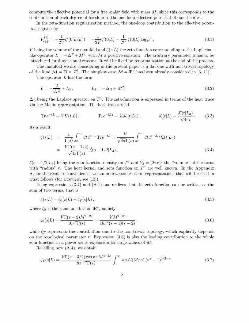
In this limit the topological contribution could indeed be arbitrarily small. In Fig. 1 the wholebehavior of the topological part of the effective potential is drawn. In order to work withdimensionless variables we have introduced the function VT (y) ≡ r4VT (r) of the dimensionlessvariable y ≡ Mr. The graphic corresponds to the exact expression for VT (y), as given e.g. bythe first lines of Eq. (3.15), multiplied by 3 · 64π2. A very smooth transition from the behaviorcorresponding to Mr ≪ 1, Eq. (3.15), to the one for Mr ≫ 1, Eq. (3.16), is revealed. In Fig. 2,the corresponding graphic of the full effective potential, Eq. (3.13), is drawn, again as a functionof y and setting µRr = 1.

At this point, the effective potential −and, as a consequence, the induced cosmologicalconstant for the models we are interested in− can be obtained by adding up several contributionsof the kind (3.13).

3.1 The multi-graviton model

We start with the explicit example of multi-graviton model given by (2.9), in which there is asingle massless graviton and (N − 1)/2 couples of massive gravitons, with masses given by

M0 = |µ0| = 0 , Mp = |µp| =πp

zc, p = 1, 2, ...,

N − 1

2. (3.17)

On the manifold M = IR × T 3, the massless graviton gives no contribution to the effectivepotential, while it does appear explicitly on manifolds with a non-vanishing curvature. Sincethe massive gravitons always show up in pairs, in order to perform the computation of theeffective potential, it is sufficient to consider only one half of the whole massive spectrum.Moreover, we have to take into account that each massive graviton contributes with five scalardegrees of freedom. After these considerations have been properly taken into account, for theeffective potential we get the following expression

Veff = 10

N−1

2∑

p=1

M4p

64π2

(

lnM2

p

µ2R

− 3

2

)

7

0.2 0.4 0.6 0.8 1 1.2y

-1

-0.8

-0.6

-0.4

-0.2

V~

THyL

Figure 1: The exact expression for VT (y) ≡ r4VT (r), multiplied by 3 · 64π2, as a function of y ≡ Mr.

−10

N−1

2∑

p=1

M4p

12π2

∫ ∞

1du G(Mpru) (u2 − 1)3/2 . (3.18)

One can see that, as for the non-compact flat case (see Ref. [6] for details), in order to have a(small) positive induced cosmological constant one has to consider a large value of N , that is,a huge number of massive gravitons. In this respect, the torus topology does not improve thesituation. As we are now going to show, this is no longer the case for the multi-supergravitonmodel.

3.2 The multi-supergraviton model

Here we have to distinguish two cases: the first one corresponds to the choice of periodic bound-ary conditions in both the bosonic and fermionic sectors. In such situation, the degrees offreedom due to bosons exactly compensate the degrees of freedom due to fermions. Moreover,for any massive boson there is a fermion with the same mass and, since the contribution to theeffective potential of any fermionic degree of freedom is opposite to the contribution of a bosonicdegree of freedom, it turns out that the induced cosmological constant vanishes, independentlyof the mass spectrum.

In the second case, that is when anti-periodic boundary conditions are imposed in thefermionic sector, the situation changes completely, since the fermionic mass spectrum becomesreally different with respect to the bosonic one. For example, by choosing N = 3 [11], thesolutions of Eqs. (2.10) and (2.12) give

M0 = 0 , M1 = M2 = m , for bosons , (3.19)

8

0.5 1 1.5 2 2.5y

-0.006-0.004-0.002

0.0020.0040.0060.008

V~

effHyL

Figure 2: The exact expression for Veff (y) ≡ r4Veff (r), Eq. (3.13), as a function of y ≡ Mr.

M0 = M2 =m√3

, M1 =2m√

3, for fermions , (3.20)

m being an arbitrary mass parameter.By taking into account the number of degrees of freedom, the one-loop effective potential

becomes, in this case

Veff =M4

1

4π2

(

lnM2

1

µ2R

− 3

2

)

− 4M41

3π2

∫ ∞

1du G(M1ru) (u2 − 1)3/2

−M40

4π2

(

lnM2

0

µ2R

− 3

2

)

+4M4

0

3π2

∫ ∞

1du G(M0ru) (u2 − 1)3/2

−M41

8π2

(

lnM2

1

µ2R

− 3

2

)

+2M4

1

3π2

∫ ∞

1du G(M1ru) (u2 − 1)3/2

= − m4

36π2log

216

39+ VT , (3.21)

VT being the sum of all the topological contributions. As one sees, the first term on the right-hand side of the latter equation is always negative, but the whole effective potential could bepositive due to the presence of the topological term. For example, in the regime mr ≪ 1, from(3.15) one has

VT ∼ 1

8π2r4=⇒ Veff > 0 for mr <

(

2

9log

216

39

)−1/4

∼ 1.4 , (3.22)

9

while in the opposite regime, mr ≫ 1, by using (3.16) one can see that the topological contri-bution although still positive it is negligible, and thus the effective potential remains negative.

In Fig. 3, the corresponding graphic of the full effective potential, Eq. (3.21), is drawn,again as a function of y ≡ mr.

0.2 0.4 0.6 0.8 1 1.2 1.4y

-0.2

-0.15

-0.1

-0.05

V~

effHyL

Figure 3: The exact expression for Veff (y) ≡ r4Veff (r), Eq. (3.21), as a function of y ≡ mr.

4 Conclusions

In this paper, we have computed the effective potential corresponding to a multi-graviton modelwith supersymmetry in the case where the bulk is a flat manifold with the topology of a torus(more precisely IR × T 3), and we have shown that the induced cosmological constant could bepositive due to topological contributions.

In previous papers [6, 11] multi-graviton and multi-supergraviton models have been con-sidered in IR4. It has been shown that in the multi-graviton model the induced cosmologicalconstant can be positive, but only if the number of massive gravitons is sufficiently large, while inthe supersymmetric case the cosmological constant can be positive if one imposes anti-periodicboundary conditions in the fermionic sector. Note that the topological effects discussed abovemay also be relevant in the study of electroweak symmetry breaking in models with a similartype of non-nearest-neighbour couplings, for the deconstruction issue [15].

In the case of the torus topology, the topological contributions to the effective potential havealways a fixed sign, depending on the boundary conditions one imposes. In fact, they are negativefor periodic fields and positive for anti-periodic fields. This means that the torus topologyprovides a mechanism which, in a most natural way, permits to have a positive cosmological

10

constant in the multi-supergravity model with anti-periodic fermions, being the value of suchconstant regulated by the corresponding size of the torus.1 In this situation one can mostnaturally use the minimum number, N = 3, of copies of bosons and fermions.

We finish with the remark that it would be interesting to apply the deconstruction scheme ofRef. [6] also for the case of two latticized extra dimensions, which in the continuous limit wouldcontain the orbifold singularity. This analysis might have a quite interesting impact on branerunning coupling calculations [17].

Acknowledgments

We thank Sergei D. Odintsov for useful discussions and suggestions. Support from the programINFN(Italy)-CICYT(Spain), from DGICYT (Spain), project BFM2003-00620, and from SEEUgrant PR2004-0126 (EE), is gratefully acknowledged.

A Zeta function on the torus

Eigenvalues of the Laplacian on the 3-dimensional torus are of the form λn = n2, n ∈ ZZ3, andthus the corresponding heat kernel is given by

K(t|L3) =e−tM2

V3

∑

n∈ZZ3

e−tn2/r2

=e−tM2

(4πt)3/2

∑

n∈ZZ3

e−π2n2r2/t , (A.1)

being V3 = (2πr)3 the “volume” of T3. Using the expression above, the zeta function of thisLaplacian can be written as

ζ(s|L3) = ζ0(s|L3) + ζT (s|L3) , (A.2)

where the contribution

ζ0(s|L3) =V3Γ(s − 3/2)M3/2−2s

(4π)3/2Γ(s), (A.3)

comes from the n = 0 term and it is the same one has for IR3, while ζT corresponds to thecontribution due to the non-trivial topology. Such term can be written in different ways, forinstance, as an infinite sum of Bessel functions.

In Refs. [12] one can find many interesting results concerning zeta functions and heat kernelscorresponding to operators on manifolds with constant curvature. In particular, on the torusone has the very nice representation

ζT (z|L3) =M3−2z sin πz

4π2(1 − z)

∫ ∞

1du G(Mru) (u2 − 1)1−z

= − πz−2

4Γ(z)

∑

n∈ZZ3;n 6=0

(

M

r|~n|

)3/2−z

K3/2−z(2πMr|~n|) , (A.4)

1A more crude analysis for the pure scalar case already hinted towards this conclusion. However, the sign issuewas there not easy to fix [16], the reason being now clear.

11

where G(x) is given by

G(x) =∑

n∈ZZ3;n 6=0

e−2π|~n|x = −1 +x

π2

∑

n∈ZZ3

1

(n2 + x2)2

= −1 +1

π2x3+

x

π2G0(x) , (A.5)

G0(x) being the regular function

G0(x) =∑

n∈ZZ3; n 6=0

1

(n2 + x2)2. (A.6)

References

[1] N. Boulanger, T. Damour, L. Gualtieri and M. Henneaux, Nucl. Phys. B597 (2001) 127,hep-th/0007220; N. Boulanger, Fortsch. Phys. 50 (2002) 858, hep-th/0111216.

[2] A. Sugamoto, Grav. Cosmol. 9 (2003) 91, hep-ph/0210235; M. Bander, Phys. Rev.D64 (2001) 105021; V. Jejjala, R. Leigh and D. Minic, Phys. Lett. B556 (2003) 71,hep-th/0212057.

[3] N. Arkani-Hamed, A.G. Cohen and H. Georgi, Phys. Rev. Lett. 86 (2001) 4757,hep-th/0104005; N. Arkani-Hamed, H. Georgi, M.D. Schwartz, Ann. Phys. (NY) 305 (2003)96, hep-th/0210184; C.T. Hill, S. Pokorski and J. Wang, Phys. Rev. D64 (2001) 105005.

[4] T. Damour, I. Kogan and A. Papazoglou, Phys. Rev. D66 (2002) 104025, hep-th/0206044;C. Deffayet and J. Mourad, Class. Quant. Grav. 21 (2004) 1833, hep-th/0311125.

[5] N. Kan and K. Shiraishi, Class.Quant.Grav. 20 (2003) 4965, gr-qc/0212113.

[6] G. Cognola, E. Elizalde, S. Nojiri, S. D. Odintsov and S. Zerbini, Mod. Phys. Lett. A19,(2004) 1435.

[7] L. Randall and R. Sundrum, Phys. Rev. Lett. 83 (1999) 3370, hep-th/9905221.

[8] M. Tegmark et al. [SDSS Collaboration], Phys. Rev. D69 (2004) 103501, astro-ph/0310723.

[9] S. Hamamoto, Prog. Theor. Phys. 97 (1997) 327, hep-th/9611141.

[10] R. Maartens, Living Rev. Rel. 7 (2004) 7, gr-qc/0312059.

[11] S. Nojiri and S. D. Odintsov, Phys. Lett. B590 (2004) 295, hep-th/04030162.

[12] E. Elizalde, S. D. Odintsov, A. Romeo, A.A. Bytsenko and S. Zerbini, Zeta Regularisation

Techniques with Applications. (World Scientific, Singapore, 1994); E. Elizalde, Ten physical

applications of spectral zeta functions (Springer, Berlin, 1995); A.A. Bytsenko, G. Cog-nola, E. Elizalde, V. Moretti and S. Zerbini, Analytic Aspects of Quantum Fields. (WorldScientific, Singapore, 2003)

[13] A.A. Bytsenko, G. Cognola, L. Vanzo and S. Zerbini. Phys. Rept. 266 (1996) 1.

12

[14] I.O. Cherednikov, Acta Phys. Slov. 52 (2002) 221, hep-th/0206245.

[15] S. Nojiri, S.D. Odintsov and A. Sugamoto, PLB590 (2004) 239, hep-th/0401203,

[16] E. Elizalde, Phys. Lett. B516 (2001) 143.

[17] K. Milton, S.D. Odintsov and S. Zerbini, PRD65, 2002, 065012, hep-th/0110051.

13