arX

iv:h

ep-t

h/07

0219

5v3

22

May

200

7

Preprint typeset in JHEP style - HYPER VERSION WIS/02/07-FEB-DPP

The Moduli Space and M(atrix) Theory of

9d N = 1 Backgrounds of M/String Theory

Ofer Aharonya,b, Zohar Komargodskia, Assaf Patira

aDepartment of Particle Physics, Weizmann Institute of Science, Rehovot

76100, IsraelbSITP, Department of Physics and SLAC, Stanford University, Stanford, CA

94305, USA

E-mail: ofer.aharony@weizmann.ac.il,

zohar.komargodsky@weizmann.ac.il, assaf.patir@weizmann.ac.il

Abstract: We discuss the moduli space of nine dimensional N = 1 supersymmetric

compactifications of M theory / string theory with reduced rank (rank 10 or rank

2), exhibiting how all the different theories (including M theory compactified on a

Klein bottle and on a Mobius strip, the Dabholkar-Park background, CHL strings

and asymmetric orbifolds of type II strings on a circle) fit together, and what are

the weakly coupled descriptions in different regions of the moduli space. We argue

that there are two disconnected components in the moduli space of theories with

rank 2. We analyze in detail the limits of the M theory compactifications on a

Klein bottle and on a Mobius strip which naively give type IIA string theory with

an uncharged orientifold 8-plane carrying discrete RR flux. In order to consistently

describe these limits we conjecture that this orientifold non-perturbatively splits into

a D8-brane and an orientifold plane of charge (−1) which sits at infinite coupling.

We construct the M(atrix) theory for M theory on a Klein bottle (and the theories

related to it), which is given by a 2 + 1 dimensional gauge theory with a varying

gauge coupling compactified on a cylinder with specific boundary conditions. We

also clarify the construction of the M(atrix) theory for backgrounds of rank 18,

including the heterotic string on a circle.

Keywords: Superstring Vacua; String Duality; M-Theory; M(atrix) Theories.

Contents

1. Introduction 1

2. The moduli space of nine dimensional N = 1 backgrounds 2

2.1 A review of nine dimensional N = 1 theories with rank 18 3

2.2 M theory on a Klein bottle and other rank 2 compactifications 8

2.3 The X background demystified 12

2.4 M theory on a Mobius strip and other rank 10 compactifications 14

3. The M(atrix) theory description of M theory on a cylinder and on

a Klein bottle 16

3.1 The M(atrix) theory of M theory on a cylinder 16

3.2 The M(atrix) theory of the Klein bottle compactification 22

3.3 The AOA limit of the M(atrix) theory 24

4. Conclusions and open questions 28

A. Spinor conventions 29

B. Periodicities of p-form fields in some 9d compactifications 30

C. Modular invariance and T-duality in the AOA partition function 31

D. Quantum mechanics of D0-branes on the Klein bottle 34

1. Introduction

In this paper we discuss in detail the structure of the moduli space of nine dimen-

sional N = 1 supersymmetric backgrounds of M theory and string theory, and their

M(atrix) theory construction. There are two main motivations for this study :

• The global structure of the moduli space of (maximally supersymmetric) toroidal

compactifications of M/string theory has been studied extensively, and all of its

corners have been mapped out. Less is known about compactifications which

preserve only half of the supersymmetry (16 supercharges).1 The moduli space

1Some of these backgrounds were studied in [1].

– 1 –

of such nine dimensional backgrounds with rank 18 (including heterotic strings

on a circle) has been extensively studied, and all its corners are understood;

however it seems that no similar study has been done for backgrounds with

lower rank (rank 10 or rank 2). These backgrounds include the compactifica-

tion of M theory on a Klein bottle and on a Mobius strip. In this paper we

study the moduli space of these backgrounds in detail. We will encounter two

surprises : we will see that the moduli space of backgrounds of rank 2 has two

disconnected components,2 and we will see that both for rank 2 and for rank

10 there is a region of the moduli space which has not previously been ex-

plored, and whose description requires interesting non-perturbative corrections

to some orientifold planes in type IIA string theory.

• The theories we discuss (with rank n) have non-trivial duality groups of the

form SO(n − 1, 1,Z). In their heterotic descriptions these are simply the T-

duality groups. However, from the M theory point of view these dualities are

quite non-trivial. In particular, it is interesting to study the manifestation of

these duality groups in the M(atrix) theory description of these backgrounds;

T-duality groups in space-time often map to interesting S-duality groups in

the M(atrix) theory gauge theories. In this paper we will derive the M(atrix)

theory for some of these backgrounds; the detailed discussion of the realization

of the duality in M(atrix) theory is postponed to future work.

We begin in section 2 with a detailed discussion of the structure of the moduli

space of 9d N = 1 backgrounds. We review the structure of the moduli space of

rank 18 backgrounds, since this will have many similarities to the moduli spaces of

reduced rank, and we then discuss in detail all the corners of the moduli spaces of

reduced rank. In section 3 we construct the M(atrix) theory for the backgrounds

corresponding to M theory on a cylinder (with a specific light-like Wilson line) and

on a Klein bottle. The case of the cylinder has been constructed before [3], but we

clarify its derivation and the mapping of parameters from space-time to the M(atrix)

theory. Our construction for the Klein bottle is new. We end in section 4 with

our conclusions and some open questions. Four appendices contain various technical

details.

2. The moduli space of nine dimensional N = 1 backgrounds

In this section we review the moduli space of compactifications of string/M theory to

nine dimensions which preserve N = 1 supersymmetry. On general grounds, if such a

compactification has a rank n gauge group in its nine dimensional low-energy effective

action, its moduli space takes the form SO(n− 1, 1,Z)\ SO(n− 1, 1)/ SO(n− 1)×R,

2This was independently discovered by A. Keurentjes [2].

– 2 –

with the first component involving n−1 real scalars sitting in n−1 vector multiplets

and the second component involving the scalar sitting (together with an additional

U(1) vector field) in the graviton multiplet. In different regions of this moduli space

there are different weakly coupled descriptions of the physics. We begin by reviewing

the n = 18 case which is well-known. We then discuss the cases of n = 2 and n = 10,

where we will encounter some surprises and some regions which have not previously

been analyzed.

2.1 A review of nine dimensional N = 1 theories with rank 18

In this subsection we review the different regions of the moduli space of nine di-

mensional compactifications of M theory and string theory with 16 supercharges

and a rank 18 group, including M theory on R9 × S1 × (S1/Z2), the two heterotic

strings compactified on a circle, the type I string on a circle and the type I’ string.

The results are mainly from [4] and [5]. The full moduli space for these theories

is SO(17, 1,Z)\ SO(17, 1)/ SO(17) × R. Naturally, different descriptions are valid in

different regions of this space. For simplicity, we shall restrict our discussion to the

subspaces of moduli space that have enhanced E8 ×E8 and enhanced SO(32) gauge

symmetries at low energies. These subspaces take the form SO(1, 1,Z)\ SO(1, 1)×R,

so they are analogous to the rank 2 case, which is the main subject of this paper,

and we will see many similarities between these two cases. However, a reader that is

familiar with rank 18 compactifications is welcome to skip to the next subsection.

We define M theory on R9 ×S1 × (S1/Z2) by periodically identifying the coordi-

nates x9 and x10 with periodicities 2πR9 and 2πR10, and also identifying x10 ≃ −x10

and requiring that the M theory 3-form Cµνρ change sign under this reflection. This

space has two boundaries/orientifold planes, at x10 = 0 and at x10 = πR10. The

orientifold breaks half of the eleven dimensional supersymmetry, leaving 16 super-

charges. This eleven dimensional orientifold is not anomaly-free: there is a gravita-

tional anomaly in the 10d theory obtained by reducing on x10 that comes from the

boundaries, and must be cancelled by additional massless modes that are restricted

to the fixed planes. As in the 10 dimensional case, part of the anomaly can be

cancelled by a generalized Green-Schwarz mechanism (using the Cµν(10) form), and

the remaining anomaly is cancelled by the addition of 496 vector multiplets. In ten

dimensions this restricts the gauge group to be either SO(32) or E8 × E8. However,

in the 11d case the anomaly must be divided equally between the two fixed planes,

so there is [4] an E8 gauge group living at each orientifold plane. When the two radii

are large (compared to the 11d Planck length), the low energy limit is described by

11d supergravity on the cylinder, coupled to two N = 1 E8 SYM theories on the two

boundaries.

In the limit where R9 is large and R10 is small, one obtains [4] the heterotic

E8 × E8 string, with string coupling gh = R3/210 and string length R

−1/210 (here and

henceforth we suppress numerical constants of order one, and measure all lengths in

– 3 –

11d Planck units). This is a valid description of the physics as long as R10 ≪ 1 and

R9 ≫ R−1/210 .

When we continue to shrink R10 to make it smaller than R−29 , we reach a point

where the x9 circle becomes small compared to the string scale. At this point we must

switch to the T-dual picture. Recall that the E8×E8 heterotic string with no Wilson

lines is T-dual to itself, with an enhanced gauge symmetry at the self-dual radius.

Thus, the appropriate description in this regime is once again the heterotic E8 ×E8

string, compactified on a circle of radius R−110 R

−19 with string coupling gh′ = R10R

−19 .

This description is valid for R10 ≪ R9 and R9 ≪ R−1/210 . In the low-energy effective

action, the E8 × E8 × U(1)2 gauge group is enhanced to E8 × E8 × SU(2) × U(1)

along the line R29R10 = 1.

This description is valid for arbitrarily small R10, so next we fix R10 and shrink

R9. This has the effect of increasing the string coupling in the T-dual heterotic

picture. For R9 ≪ R10 we open up an extra dimension (as above) and get another

region of moduli space that is also described by M theory on a cylinder. The length

of the dual cylinder is R1/210 R

−19 , the radius is R−1

10 R−19 and the Planck length of

this “other M theory” is (lp)M ′ = R−1/39 R

−1/610 . Thus, this description is valid for

R9 ≪ R10 ≪ R−4/59 .

We are left with the region of R10 ≫ R−4/59 and R9 ≪ 1. This region is covered

by the backgrounds that we get by reducing M theory on the periodic direction of

the cylinder. This theory is known as type I’ strings [6], and it may be viewed as

an orientifold of type IIA string theory, obtained by dividing by worldsheet parity

together with x9 → −x9. The fixed points are now orientifold 8-planes (O8 planes)

of type O8−, which carry (−8) units of D8-brane charge. Tadpole cancellation then

requires that this background must include also 16 D8-branes.

Another way to obtain the same type I’ theory is as the T-dual of type I string

theory. This is helpful in understanding an important feature of this background [5].

In type I strings, there are two diagrams that contribute to the dilaton tadpole –

the disk and the projective plane – and these diagrams conspire to cancel, homoge-

neously throughout space-time. On the other hand, in type I’ string theory there are

two identical O8 planes at the boundaries, and 16 D8-branes that are free to move

between the boundaries. As a result tadpole cancellation does not occur locally in

this theory: the oriented disk diagram gets a contribution that is localized at the

D8-branes, while the unoriented projective plane diagram gets contributions local-

ized at the orientifold planes. Each D-brane cancels one-eighth of the contribution

of an orientifold plane, and there is generally a gradient for the dilaton, whose exact

form depends on the configuration of D8-branes.

The configuration of the branes between the orientifold planes also determines

the low-energy gauge group of the background. One possible configuration of D-

branes is to have 8 D8-branes on each O8 plane. In this case the dilaton is constant

and there is an SO(16) gauge group at each of the boundaries. In all other cases

– 4 –

the dilaton varies between the orientifold planes and the D-branes, and between

the D-branes, with a gradient proportional to the inverse string length and to the

local ten-form charge. This dilaton gradient causes the dilaton to diverge when the

distance between two such planes is of order g−1I′ ls (where gI′ is the string coupling

somewhere in the interval), imposing restrictions on the length of the interval and

on the distances between the orientifold planes and the D-branes.

The last piece of information on type I’ string theory that we need is that when

the string coupling becomes infinite on one of the orientifold planes, there may be

D0-branes that become massless there [7, 8, 9]. If there are n D8-branes on this

orientifold plane, then these additional light degrees of freedom conspire to enhance

the SO(2n) gauge group to En+1. Specifically, in order to get an E8 gauge group in

this theory, we need to put 7 D8-branes on an orientifold plane, and one D8-brane

away from it, precisely at a distance that will maintain the infinite string coupling

at the O8 plane. If we do this at both ends (schematically: (O8+7D8)-D8-D8-

(O8+7D8)) we get an E8 × E8 × U(1) × U(1) gauge group (in nine dimensions),

providing the vacuum of type I ′ string theory that is dual to the heterotic E8 × E8

string with no Wilson line turned on. The distance in string units between the two

single D8-branes will be denoted by xI′ .

After this detour on the general properties of type I’ string theory, let us now

return to the compactification of M theory to this background. We can reach a type

I’ background in two ways: starting with the original M theory and reducing on x9,

or starting from the dual M theory and reducing on the periodic direction there.

Both constructions give us a type I ′ theory in its E8 × E8 vacuum, with couplings:

gI′1 = R3/29 (ls)I′1 = R

−1/29 RI′1 = R10 (2.1)

gI′2 = R−19 R

−5/410 (ls)I′2 = R

1/410 RI′2 = R

1/210 R

−19 (2.2)

Note that we need to be careful about what we mean by gI′, since the string coupling

varies along the interval and diverges at the boundaries; what we will mean by gI′

(here and in other cases with a varying dilaton) is the string coupling somewhere in

the interior of the interval, and the differences between different points in the interval

are of higher order in gI′ so our expression is true in the weak gI′ limit (which is the

only limit where g is well-defined anyway). Naively, the first description is valid (ex-

cept near the orientifold planes where the string coupling diverges) whenever R9 ≪ 1

and R10 ≫ R−1/29 , and the second description is valid whenever R10 ≫ R

−4/59 and

R10 ≫ R49, but this would give an overlapping range of validity to the two differ-

ent descriptions (which would also overlap with some of our previous descriptions).

However, requiring that the distance between each D8 and the O8 should be such

that the orientifold plane is at infinite coupling, we find xI′ in the two cases to be

1) xI′1 = (R10R29 − 1)R

−3/29 (2.3)

2) xI′2 = (1 − R29R10)R

−19 R

1/410 (2.4)

– 5 –

Now, the regime of validity for each of the type I ′ backgrounds (defined by (gs)I′ ≪ 1

and xI′ ≥ 0) is distinct; the first description is valid when R9 ≪ 1 and R10 ≤ R−29

and the second description is valid when R10 ≫ R−4/59 and R10 ≥ R−2

9 . Furthermore,

at the line R10R29 = 1, which was the line of enhanced symmetry in the heterotic

E8 × E8 string theory, we have xI′ = 0 for both backgrounds. On this line the two

D8-branes coincide, enhancing the U(1) × U(1) symmetry to SU(2) × U(1) exactly

as in the heterotic case. This implies that the two type I ′ backgrounds are actually

related by an SU(2) gauge transformation, which is consistent with the fact that

xI′1/(ls)I′1 = −xI′2/(ls)I′2. We see that the line R10R29 = 1 continues to be a line of

enhanced symmetry throughout the moduli space.

The backgrounds described thus far cover the whole moduli space of nine dimen-

sional N = 1 backgrounds with an E8 × E8 gauge group. The top graph in figure 1

displays how these backgrounds fill in all possible values of the radii of the M theory

we started with. Of course, the top part of this figure (above the dashed line) is

related by an SU(2) gauge transformation to the bottom part, so the true moduli

space is just half of this figure (above or below the dashed line).

Next, we turn to the subspace of the rank 18 backgrounds with an unbroken

SO(32) gauge symmetry.3 This subspace includes the type I ′ background in its

SO(32) vacuum. This vacuum is obtained by having all 16 D8-branes sit at one of

the O8− planes (so that it has the same charges as an O8+ plane). The dilaton then

grows as we go from this O8− plane to the other one. We denote the distance between

the orientifold planes as RI′ (in string units) and the string coupling (defined, for

instance, near the O8− plane with the branes) as gI′. The regime of validity of this

description is 1 ≪ RI′ ≪ g−1I′ .

For RI′ ≪ 1, we need to switch to the T-dual of this description, which is the

type I background with no Wilson lines. The string coupling in type I is gI = gI′/RI′

and the radius of the compact circle is RI = R−1I′ . This description is thus valid for

gI′ ≪ RI′ ≪ 1.

As we further decrease RI′ we increase the coupling of the type I string the-

ory, and eventually we should go over to the S-dual heterotic SO(32) string. The

parameters of this heterotic background are gh = RI′/gI′ and Rh = 1/RI′, and

its string length is (ls)h = (gI′/RI′)1/2, implying that it is a valid description for

RI′ ≪ gI′ ≪ R−1I′ .

On the line gI′ = R−1I′ we find Rh = (ls)h. This is a line of self T-duality and

enhanced SU(2) gauge symmetry in the heterotic SO(32) string. We can now move

to the T-dual picture, obtaining another heterotic SO(32) description. By going to

the strong coupling limit of the new heterotic background, we get another type I

background, and by another T-duality we get another regime described by the type

3Actually we will only describe one connected component of this subspace, which will turn out

to be analogous to the rank 2 case. The other component has a discrete Wilson line that is only

felt by spinor representations of SO(32).

– 6 –

0 10

1

R9

R10

Het−E8× E

8

Het−E8× E

8

M/C2

M/C2

I’E

8× E

8I’

E8× E

8

0 1 0

1

RI’

g I’

I’SO(32)

type I

Het−SO(32)

I’SO(32)

type I

Het−SO(32)

Figure 1: The E8 ×E8 and SO(32) subspaces of the moduli space of rank 18 compactifi-

cations of M theory and string theory. In the first graph the parameters are the period and

length of the cylinder in Planck units as defined for the upper right compactification of M

theory on a cylinder, and in the second they are the distance between the orientifold planes

in units of the string length, and the string coupling on the O8− plane with the branes on

it, of the type I’ background appearing in the lower right corner. The dashed line in both

graphs is the line of enhanced SU(2) symmetry; the regions of the graphs below and above

this line are identified.

I ′ background. These three types of backgrounds cover the whole SO(32) subspace

of the moduli space, as presented in the second graph of figure 1.

In the heterotic SO(32) description we found that along the line RI′ = g−1I′ a

U(1) symmetry gets enhanced to SU(2), by the usual mechanism of a winding mode

– 7 –

becoming massless at the self-dual point. As in the previous example, the same

enhancement occurs on this line also in other regions of the moduli space. In the

type I ′ description, this is the line where the O8 plane without the branes is at

infinite coupling. The half-D0-branes that live on the orientifold plane then become

massless at this line, and they are responsible for the symmetry enhancement (from

U(1) to E1 = SU(2)) in this description.

It is important to remember that the two branches depicted in figure 1 are just

specific subspaces of the moduli space of rank 18 theories and that the rest can be

reached by turning on Wilson lines in the heterotic or type I pictures, or equivalently

moving around D8-branes in the type I ′ picture. Thus, the two plots in the figure

are just two slices of the full moduli space. This is important to emphasize since in

the next subsection a similar picture will arise, but in that case there are no Wilson

lines to be turned on, so the two branches are actually two disconnected components

of the 9d moduli space.

2.2 M theory on a Klein bottle and other rank 2 compactifications

We now wish to repeat the above analysis for M theory compactified on a Klein

bottle (first considered in [10]) instead of a cylinder. One may start by asking if

M theory makes sense at all on a Klein bottle. We will see that the answer is yes,

and that this background arises as a strong coupling limit of consistent string theory

backgrounds.

Let us begin by considering type IIB string theory gauged by the symmetry

group Z2 = 1, H9Ω, where Ω is worldsheet parity and H9 is a shift in the 9th

coordinate,

H9Ω :

Xµ(z, z) ≃ Xµ(z, z), µ 6= 9

X9(z, z) ≃ X9(z, z) + 2πR9.(2.5)

This orientifold theory is derived by imposing H9Ω = 1 on the spectrum of the IIB

theory compactified on a circle of radius 2R9; this breaks half of the supersymmetry

(one of the gravitinos is projected out and the other one remains). In this case there

are no fixed planes, and one does not need to add D-branes to cancel any tadpole,

as explained in [10]. We refer to this background as the Dabholkar-Park background

or the DP background.

We can compactify the DP background on an additional circle of radius R8 in

the x8 direction, and T-dualize in this direction. Because of the orientation reversal

in the original DP background, the resulting background is type IIA string theory

gauged by

Xµ(z, z) ≃ Xµ(z, z), µ 6= 8, 9

X ′8(z, z) ≃ −X ′8(z, z),

X9(z, z) ≃ X9(z, z) + 2πR9.

(2.6)

– 8 –

Thus, this describes a type IIA compactification on a Klein bottle (K2) of area

(2πR8)× (2πR9), where R8 = l2s/R8, with an orientation reversal operation (see also

[11]).4 One can lift this theory to a background of M theory in the usual way by

taking the strong coupling limit (the supersymmetry of this background prohibits

a potential for the dilaton). The worldsheet parity is identified in M theory with

flipping the sign of all components of the 3-form field. Thus, as promised, M theory

on a Klein bottle naturally arises as a strong coupling limit of a string theory.

Consider now M theory compactified on a Klein bottle of radii K2(R10, R9)

measured in Planck units, namely with the identification

(X10, X9) ≃ (−X10, X9 + 2πR9), (2.7)

including a reversal of the 3-form field, and also with X10 periodically identified with

radius R10. If we shrink R10 we get a background that is described in detail in [12]

and [13] (additional related analysis can be found in [14]). This background can be

defined as type IIA string theory with a gauging of the symmetry

(−)FL × (X9 → X9 + 2πR9), (2.8)

where FL is the space-time fermion number of the left-moving fields on the world-

sheet. We refer to this background as the asymmetric orbifold of type IIA or AOA.

The type IIA string coupling is gs ≃ R3/210 , and ls ≃ R

−1/210 .

If we continue to shrink R10, the circle becomes small (in string units) and we

need to change to the T-dual description. It was noticed in [12] that the AOA back-

ground has an enhanced SU(2) symmetry point when R9 = ls/√

2, and in [13] it

was demonstrated that (as implied by this enhanced symmetry) this background is

actually self-T-dual. In appendix C we explicitly evaluate the partition function of

this model, showing that it is modular invariant and respects the T-duality. There-

fore, when we continue to shrink R10 we should switch to a T-dual AOA description,

which has (R9)T ≃ 1/R9R10 and (gs)T ≃ R10/R9. This dual AOA description can

in turn be lifted to a dual M theory on a Klein bottle. The regimes of validity of

these different descriptions are exactly the same (up to numerical constants of order

one) as those we found in the previous subsection, with M theory on the Klein bottle

replacing M theory on a cylinder, and the AOA background replacing the heterotic

E8 × E8 string.

Going back to M theory on a Klein bottle, what happens if we shrink R9? Naively,

we get a theory that is an orientifold of IIA on an S1/Z2, with some boundary con-

ditions at the fixed planes. However, we have a Z2 symmetry that exchanges the two

boundaries, and since there cannot be any tadpole for the RR 10-form, we can only

4The orientation reversal leads to various periodicity conditions for the p-form fields, that are

explained in detail in appendix B.

– 9 –

have neutral orientifold planes (with respect to the 10-form charge) at the bound-

aries, unlike the standard O8− planes (which carry (−8) units of charge) and O8+

planes (which carry +8 units of charge).5 For now we conjecture that the reduction

in this direction leads to a background which we call the X-background, and that

the line of enhanced symmetry R10R29 = 1 is also a line of enhanced symmetry in

the X-background. Thus, the two remaining regions of the moduli space are covered

by the X-background and its dual (obtained by reducing the dual M theory on the

periodic cycle). In §2.3 we shall propose a stringy description of this background.

The theories described above (starting with M theory on a Klein bottle) cover

a complete moduli space of the form SO(1, 1,Z)\ SO(1, 1) × R, as shown on the top

graph of figure 2. However, there are several additional string backgrounds with 16

supercharges and a rank 2 gauge symmetry that were not included so far, so they

must be in a separate component of the moduli space. The first is the DP background

described above. Next, there is the orientifold of type IIA on an interval S1/Z2, with

an O8− plane on one end and an O8+ plane on the other [15]. We refer to this

background as the O8± background, and denote the length of the interval in string

units by πR±. No D-branes are required for tadpole cancellation here. However,

the dilaton does have a gradient (identical to that in the SO(32) background of

the type I ′ string) that puts a limit on the maximum length of the interval, of the

form R± < 1/g± (where g± is again defined as the string coupling somewhere in

the interval). This background was studied in [15], where it was shown to be T-

dual to the DP background. An important feature of this background is that when

the distance between the orientifold planes is such that the coupling on the O8−

is infinite, there are half-D0-branes stuck on the orientifold that become massless.

Locally, this is exactly the same as in the type I ′ SO(32) vacuum; in both cases the

fractional branes enhance the U(1)2 symmetry to SU(2) × U(1).

Finally, one other background can be obtained by gauging type IIB string theory

by the symmetry (2.8). We call this background the Asymmetric Orbifold of type

IIB or AOB. Recalling the following property of IIB strings

(−1)FL = SΩS (2.9)

(where S is the S-duality transformation of type IIB string theory) and applying

the adiabatic argument of [14], we see that this background is S-dual to the DP

background. Exactly like the AOA background, the AOB background is self-T-dual

[13] and has an enhanced SU(2) symmetry when the radius of the circle is ls/√

2.

We can now describe the second component of the moduli space. Start with the

O8± background with string coupling g± and radius R± (measured in string units).

5Notice that this contradicts a suggestion occasionally found in the literature, that in this limit

we get a background defined by IIA on an S1/Z2 with an O8− plane on one end and an O8+ plane

on the other.

– 10 –

0 10

1

R9

R10

M/K2

M/K2

AOA

AOA

XX

0 1 0

1

R±

g ±

O8±DP

AOB

O8±

DP

AOB

Figure 2: The two disconnected components of the moduli space including the back-

grounds of subsection 2.2. In the first graph the parameters are the periods of the Klein

bottle in Planck units as defined in (2.7) for the upper right M theory description. In the

second graph, the parameters are the radius of the circle in string units and the string

coupling (in the middle of the interval) for the O8± background on the lower right corner.

The dashed line in both graphs is the line of enhanced SU(2) gauge symmetry, and the

backgrounds below the line are identified with the backgrounds above the line.

This is a valid description for g± ≪ 1/R± and R± ≫ 1. As we decrease R±, we

need to T-dualize, as in [15], and we get the DP background with radius6 1/R±

and string coupling g±/R±. The DP description is valid as long as g± ≪ R± ≪ 1.

We can further decrease R± to the point where the DP string coupling is too large.

6We continue to ignore numerical constants of order one.

– 11 –

At this point we turn to the S-dual picture, which is the asymmetric orbifold of

type IIB (AOB). The string coupling is now R±/g±, and the S-dual string length is

(g±/R±)1/2, such that the radius 1/R± in string units is now (g±R±)−1/2. This is a

good description for g± ≪ 1/R± and R± ≪ g±.

We continue next by increasing g± to the point where the AOB radius becomes

small. Then we must use the self T-duality of this background to arrive at a dual

AOB description, with radius (g±R±)1/2 (in units of its string length) and string

coupling g−1/2± R

3/2± . This description is good for g± ≫ 1/R± and g± ≫ R3

±. The

next step is to take the S-dual of the dual AOB background. This gives another

DP background with radius (in units of its string length) g3/4± R

−1/4± and coupling

g1/2± R

−3/2± . This description is valid for g± ≫ R

1/3± and g± ≪ R3

±. The last step is to

T-dualize the new DP background to a dual O8± background, with radius g−3/4± R

1/4±

(in units of its string length) and coupling g−1/4± R

−5/4± . This description is valid for

g± ≪ R1/3± and g± ≫ 1/R±.

These six string theories cover the entire range of values of (g±, R±). The reader

should notice that the line of enhanced SU(2) symmetry in the O8± background,

R± ∼ 1/g±, smoothly goes into the line of enhanced SU(2) symmetry of the AOB

background [12], as in the previous cases we discussed.

Figure 2 summarizes the structure of the moduli space. As promised, it has

two disconnected components in the nine dimensional sense. Note that the nine

dimensional low-energy effective action on the two components is identical, but the

massive spectrum is different. The components can be related by compactifying

on an additional circle and performing a T-duality, but they are not connected as

nine dimensional backgrounds. There is an obvious relation between each of these

components and one of the subspaces of the moduli space of rank 18 compactifications

discussed in the previous subsection and depicted in figure 1.

2.3 The X background demystified

In the previous subsection we left open the description of the limit of the Klein bottle

where R9 is small and R10 is large. In this limit the Klein bottle geometrically looks

as in figure 3 (though the geometric description is not really valid at distances smaller

than the 11d Planck scale). This limit should correspond to some 10 dimensional

string theory; let us collect some features of this theory:

Figure 3: In the X region, the Klein bottle looks like a long tube between two cross-caps.

– 12 –

• After reducing M theory on the small circle R9, we expect to obtain a type IIA

string theory that lives on R8,1 × I where I is an interval. On each boundary

of the interval we should have an orientifold plane; however these orientifold

planes are non-standard because the orientifolding is accompanied by a half-

shift on the M theory circle. This half-shift modifies, among other things, the

properties of D0-branes near the orientifold. One can think of this shift as a

discrete RR flux characterizing the orientifold plane, which changes its charge

from the usual charge of (−8) to zero [16]. We will denote such orientifold

planes by O80.

• The fact that the orientifold carries no D8-brane charge is consistent with

tadpole cancellation of the 10-form field and the dilaton. Note that there is a

Z2 symmetry exchanging the two ends of the interval, so the two orientifold

planes must carry the same charge (unlike the case in the O8± background

described in the previous subsection).

• Naively one expects that in the limit of small R9 the 10 dimensional string

theory can be made very weakly coupled, and the description should involve

the usual type IIA string theory, at least far from the boundaries of the interval

(where there may or may not be large quantum corrections). We will see that

there are some regions of the moduli space where this naive expectation fails.

• The discussion of the previous subsection suggests that we should have an

enhanced SU(2) gauge symmetry when the interval is of size R ∼ 1/gs (in type

IIA string units). One may expect this enhanced symmetry to come from half-

D0-branes on the orientifold planes, as in some of the examples discussed in

the previous subsections. However, since we have a Z2 symmetry relating the

two orientifolds, it is hard to imagine how the U(1)2 group would be enhanced

to U(1) × SU(2) rather than to the more symmetric SU(2)2.

The last item above suggests some modification of the naive picture of this

background. The picture that we will suggest for the correct description of this

background is based on two facts :

• In our analogy between the rank 18 and the rank 2 theories, the X background

plays the same role as the type I ′ E8 × E8 background. In this background

the two orientifold planes are always at infinite coupling, and the enhanced

SU(2) symmetry arises when two D8-branes in the middle of the interval come

together [9].

• In some cases, when a standard (O8−) orientifold plane of charge (−8) is at

infinite coupling, it can emit a D8-brane into the bulk, leaving behind an ori-

entifold plane of charge (−9) which has no perturbative description (and which

– 13 –

always sits at infinite coupling). This phenomenon cannot be seen in pertur-

bation theory, but it can be deduced from an analysis of D4-brane probes [7].

Our suggestion is that each O80 plane non-perturbatively emits a D8-brane and

becomes an O8(−1) plane which always sits at infinite coupling. The moduli space

and 10-form fluxes of this system are then identical to those of the E8 × E8 type I ′

background, with the O8(−1) plane playing the same role as the O8− plane with 7

D8-branes on it. Now, the gauge symmetry is enhanced to SU(2) in a Z2-symmetric

manner, when the D8-branes meet in the middle of the interval, and this enhancement

is perturbative (it can happen at weak coupling). Denoting the string coupling in

the region between the two emitted D8-branes by gs (it does not vary in the interval

between the D8-branes), the distance of each brane from the respective O8(−1) plane

is ∼ 1/gs. Thus, when the branes meet, our interval indeed has a size proportional

to 1/gs as required.

We suggest that this is the correct description of O80 orientifold planes. Note

that such a large non-perturbative correction to the description of high-dimensional

orientifold planes is not surprising; already in the case of O7 planes it is known

[17] that they non-perturbatively split into two 7-branes, and the corrections to O8

planes are expected to be even larger. Our suggestion implies non-trivial corrections

to compactifications of M theory involving crosscaps (similar corrections in M theory

should also occur in a compactification on a Mobius strip, as will be discussed in the

next subsection). These corrections are similar to the ones that occur for M theory

on a cylinder with no Wilson lines. Note that when we are close to the enhanced

SU(2) point, the corrections to the naive M theory picture shown in figure 3 are not

just localized near the cross-caps as one may naively expect, but the string coupling

actually varies along the whole interval.

In order for this proposal to be consistent, there should be no massless fractional

D0-branes on the O8(−1) planes, which would lead to more enhanced symmetries than

we need. Because of the shift in the M theory circle involved in the orientifolding,

the radius of the cross-cap is actually half of the radius of the M theory circle in

the bulk, which implies that only even momentum modes (in units of the minimal

momentum on a standard orientifold plane) are allowed there. Hence, there are no

half D0-branes in backgrounds with O80 orientifolds (or O8(−1) orientifolds).

2.4 M theory on a Mobius strip and other rank 10 compactifications

There is one additional disconnected component of the moduli space of nine dimen-

sional compactifications with N = 1 supersymmetry. Consider the heterotic E8×E8

string compactified to nine dimensions on a circle of radius R9. One can consider an

orbifold of this theory generated by switching the two gauge groups together with

a half-period-shift of x9. This theory is known as the CHL string; as usual one

should add twisted sectors for the consistency of the orbifold (for more details see

– 14 –

[18, 19]). This leads to a nine dimensional compactification with a rank 10 gauge

group. We will focus on the subspace of the moduli space of this theory in which the

E8 symmetry is unbroken.

An orbifold of the E8 × E8 heterotic string on a circle can also be viewed as an

orbifold of M theory compactified on a cylinder. Begin with M theory compactified

on the cylinder

x9 ≃ x9 + 2πR9 , x10 ∈[−π

2R10,

π

2R10

]. (2.10)

The action on the heterotic string which we described above lifts in M theory to

x9 ≃ x9 + πR9 , x10 ≃ −x10. (2.11)

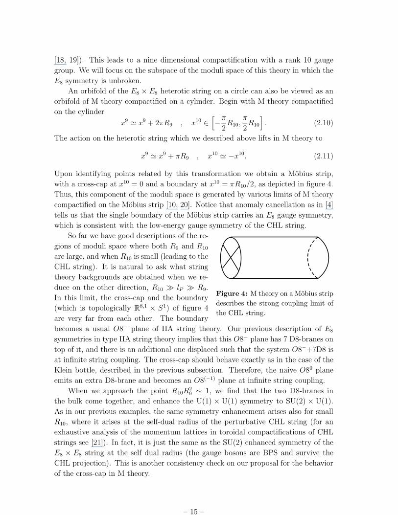
Upon identifying points related by this transformation we obtain a Mobius strip,

with a cross-cap at x10 = 0 and a boundary at x10 = πR10/2, as depicted in figure 4.

Thus, this component of the moduli space is generated by various limits of M theory

compactified on the Mobius strip [10, 20]. Notice that anomaly cancellation as in [4]

tells us that the single boundary of the Mobius strip carries an E8 gauge symmetry,

which is consistent with the low-energy gauge symmetry of the CHL string.

So far we have good descriptions of the re-

Figure 4: M theory on a Mobius strip

describes the strong coupling limit of

the CHL string.

gions of moduli space where both R9 and R10

are large, and when R10 is small (leading to the

CHL string). It is natural to ask what string

theory backgrounds are obtained when we re-

duce on the other direction, R10 ≫ lP ≫ R9.

In this limit, the cross-cap and the boundary

(which is topologically R8,1 × S1) of figure 4

are very far from each other. The boundary

becomes a usual O8− plane of IIA string theory. Our previous description of E8

symmetries in type IIA string theory implies that this O8− plane has 7 D8-branes on

top of it, and there is an additional one displaced such that the system O8−+7D8 is

at infinite string coupling. The cross-cap should behave exactly as in the case of the

Klein bottle, described in the previous subsection. Therefore, the naive O80 plane

emits an extra D8-brane and becomes an O8(−1) plane at infinite string coupling.

When we approach the point R10R29 ∼ 1, we find that the two D8-branes in

the bulk come together, and enhance the U(1) × U(1) symmetry to SU(2) × U(1).

As in our previous examples, the same symmetry enhancement arises also for small

R10, where it arises at the self-dual radius of the perturbative CHL string (for an

exhaustive analysis of the momentum lattices in toroidal compactifications of CHL

strings see [21]). In fact, it is just the same as the SU(2) enhanced symmetry of the

E8 × E8 string at the self dual radius (the gauge bosons are BPS and survive the

CHL projection). This is another consistency check on our proposal for the behavior

of the cross-cap in M theory.

– 15 –

0 10

1

R9

R10

M/Mobius

M/Mobius

CHL

CHL

1/2 X 1/2 X

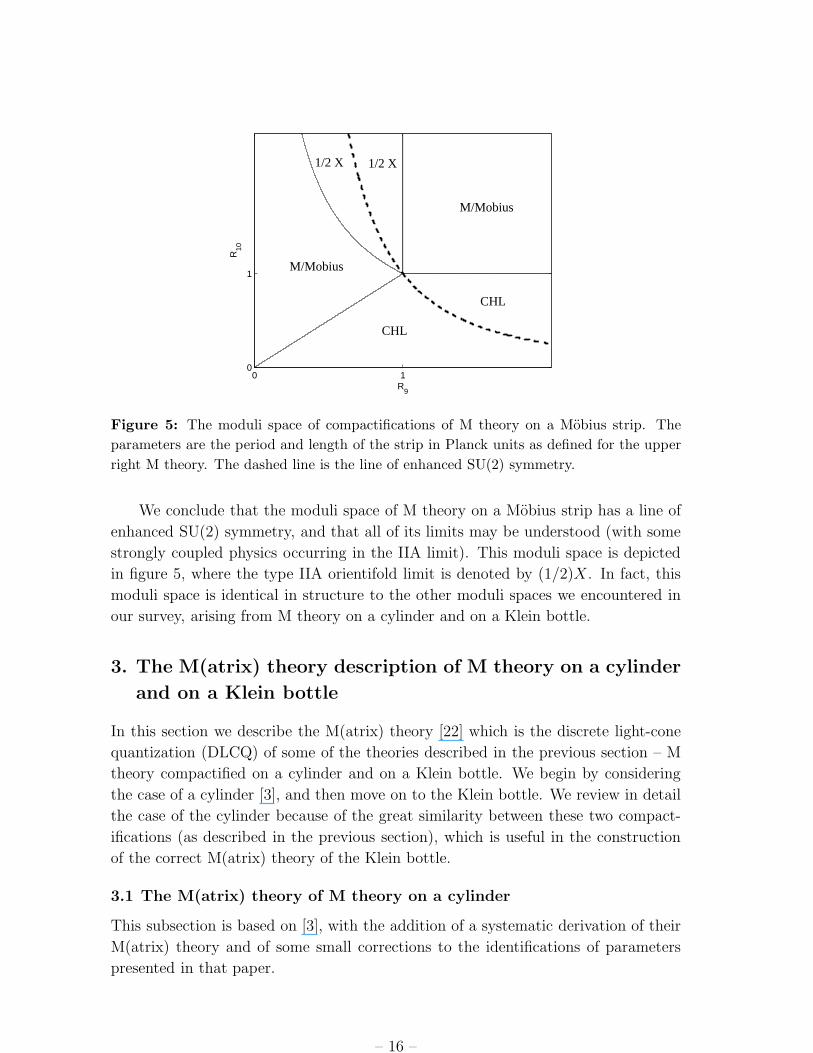
Figure 5: The moduli space of compactifications of M theory on a Mobius strip. The

parameters are the period and length of the strip in Planck units as defined for the upper

right M theory. The dashed line is the line of enhanced SU(2) symmetry.

We conclude that the moduli space of M theory on a Mobius strip has a line of

enhanced SU(2) symmetry, and that all of its limits may be understood (with some

strongly coupled physics occurring in the IIA limit). This moduli space is depicted

in figure 5, where the type IIA orientifold limit is denoted by (1/2)X. In fact, this

moduli space is identical in structure to the other moduli spaces we encountered in

our survey, arising from M theory on a cylinder and on a Klein bottle.

3. The M(atrix) theory description of M theory on a cylinder

and on a Klein bottle

In this section we describe the M(atrix) theory [22] which is the discrete light-cone

quantization (DLCQ) of some of the theories described in the previous section – M

theory compactified on a cylinder and on a Klein bottle. We begin by considering

the case of a cylinder [3], and then move on to the Klein bottle. We review in detail

the case of the cylinder because of the great similarity between these two compact-

ifications (as described in the previous section), which is useful in the construction

of the correct M(atrix) theory of the Klein bottle.

3.1 The M(atrix) theory of M theory on a cylinder

This subsection is based on [3], with the addition of a systematic derivation of their

M(atrix) theory and of some small corrections to the identifications of parameters

presented in that paper.

– 16 –

M(atrix) theory is the discrete light-cone quantization of M theory backgrounds

[23]; it provides the Hamiltonian for these theories compactified on a light-like circle,

with N units of momentum around the circle. In general, such a DLCQ description

is very complicated. However, in some M theory backgrounds it simplifies, because a

light-like circle may be viewed [24, 25] as a limit of a very small space-like circle, and

M theory on a very small space-like circle is often very weakly coupled. This leads

to a simple description of the DLCQ Hamiltonian, in which most of the degrees of

freedom of M theory decouple. In particular, this is the case for the M(atrix) theory

of M theory itself, which is given just by a maximally supersymmetric U(N) quantum

mechanical gauge theory, and for the M(atrix) theory of M theory compactified on a

two-torus, which is given by the maximally supersymmetric U(N) 2 + 1 dimensional

gauge theory, compactified on a dual torus.

The generic simplicity of M(atrix) theory is based on the fact that M theory

compactified on a small space-like circle becomes a weakly coupled type IIA string

theory. However, when boundaries are present in the M theory compactification, they

usually destroy this simplicity. For instance, as is evident from figure 1, if we take

M theory on S1/Z2 and compactify it further on a very small space-like circle, we do

not obtain a weakly coupled background (but, rather, we obtain M theory on a dual

cylinder). Thus, generically the DLCQ of M theory backgrounds with boundaries is

very complicated. However, there is an extra degree of freedom one can use in the

DLCQ constructions, which is a Wilson line along the light-like circle; such a Wilson

line becomes irrelevant in the large N limit of M(atrix) theory in which it provides a

light-cone quantization of the original background (without the light-like circle), but

it can have large effects for finite values of N . In the case of M theory on S1/Z2, as we

discussed above, the theory compactified on an additional small circle is generally

strongly coupled (see [26] for a recent discussion), except when we have a Wilson

line breaking the E8 × E8 symmetry to SO(16) × SO(16). The moduli space of this

subspace of compactifications on a cylinder is drawn in figure 6; as can be seen in

this figure, the limit of a small space-like circle leads in this case to a weakly coupled

type I string theory (with a Wilson line breaking SO(32) to SO(16)× SO(16)). The

M(atrix) theory for M theory on an interval with this specific light-like Wilson line is

then again a simple theory [27, 28, 29, 30, 31] – the decoupled theory of N D1-branes

in this type I background, which is simply an SO(N) 1 + 1 dimensional N = (0, 8)

supersymmetric gauge theory on a circle, coupled to 32 real left-moving fermions in

the fundamental representation (coming from the D1-D9 strings), half of which are

periodic and half of which are anti-periodic [5].

Now we can move on to the case we are interested in, which is the M(atrix)

theory of M theory on R9 × S1 × (S1/Z2), with an arbitrary Wilson line W for

the E8 × E8 gauge group on the S1. To construct the M(atrix) theory we should

again consider the limit of this theory on a very small space-like circle [24, 25], with

a particular scaling of the size of the cylinder as the size of this extra circle goes

– 17 –

0 10

1

R9

R10

Het−E8× E

8

Het−SO(32)

M/C2

Type I

Type I’

Figure 6: The subspace of the moduli space of M theory on a cylinder, where all back-

grounds include a Wilson line breaking the gauge group to SO(16) × SO(16). The param-

eters in the plot are the period R9 and length R10 of the cylinder in Planck units.

to zero. Again, in general this limit gives a strongly coupled theory, except in the

case where we have an additional Wilson line breaking the E8 × E8 gauge group to

SO(16)×SO(16) on the additional circle (the original Wilson line W must commute

with this Wilson line in order to obtain a weakly coupled description).7 In such a

case we obtain precisely the theory described in the previous paragraph, compactified

on an additional very small circle with a Wilson line W (which is the translation of

the original Wilson line from the E8 × E8 variables of the original M theory to the

SO(32) variables of the dual type I background). Since the additional circle is very

small we need to perform a T-duality on this circle. We then obtain a type I ′ theory

of the type described in the previous section, still compactified on a circle with the

SO(16) × SO(16) Wilson line, and with the positions of the D8-branes determined

by the eigenvalues of the Wilson line W . The D1-branes we had before now become

D2-branes which are stretched both along the interval between the orientifold planes

and along the additional circle.

The usual derivation of M(atrix) theory [24, 25] shows that the M(atrix) theory

is precisely the decoupled theory living on these D2-branes, in the limit that the

string mass scale goes to infinity keeping the Yang-Mills coupling constant on the

D2-branes, which is proportional to

g2Y M ∝ gs/ls, (3.1)

7In principle we could also have a light-like Wilson line for the other two U(1) gauge fields

appearing in the low-energy nine dimensional effective action, but we will not discuss this here.

– 18 –

fixed. The D2-brane lives on a cylinder, with a circle of radius R1 (related to the

parameters of the original M theory background by R1 = l3p/R10R , where 1/R is

the energy scale associated with the light-like circle) and an interval of length πR2

(given by R2 = l3p/R9R). In the standard case of toroidal compactifications, only

the disk contributions to the D2-brane action survive in this limit, giving a standard

supersymmetric Yang-Mills theory, with Yang-Mills coupling g2Y M = R/R9R10. How-

ever, in our case it turns out that some contributions to the D2-brane action from

Mobius strip diagrams also survive; this is evident from the fact that gs in the type

I ′ background is generally not a constant, leading through (3.1) to a non-constant

Yang-Mills coupling. This was taken into account in [3], where the Lagrangian for

any distribution of D8-branes was obtained, and it was shown that the Mobius strip

contributions are crucial to cancel anomalies in the gauge theory.

There is one special case when the Mobius contributions are absent; this is the

case when the type I ′ background has a constant dilaton, with eight D8-branes

on each orientifold plane. According to the discussion above, this case provides

the DLCQ description of M theory on a cylinder with a Wilson line breaking the

gauge symmetry to SO(16) × SO(16) (so that we are at some point on the moduli

space of figure 6), and with an additional light-like Wilson line which breaks the

gauge symmetry in the same way. We begin by describing this special case. In

this case the theory on the D2-branes away from the orientifold planes is just the

standard maximally supersymmetric 2+1 dimensional U(N) Yang-Mills theory, with

a gauge coupling related to the parameters of the original M theory background by

g2Y M = R/R9R10 (which is the same relation as in toroidal compactifications). The

field content of this theory includes a gauge field Aµ, seven scalar fields Xj and eight

Majorana fermions ψA. The boundary conditions project the U(N) gauge group to

SO(N). In addition, the D2-D8 strings give rise to 8 complex chiral fermions in

the fundamental representation χk (k = 1, · · · , 8) at the boundary x2 = 0 and 8

additional fermions χk (k = 1, · · · , 8) at the other boundary x2 = πR2. The action

is given by

S =

∫dt

∫ 2πR1

0

dx1

[ ∫ πR2

0

dx2 1

2g2YM

Tr

(− 1

2FµνF

µν + (DµXj)2+

+1

2[Xj , X i][Xj, X i] + iψAγ

αDαψA − iψAγiAB[Xi, ψB]

)+

+ i8∑

k=1

χk(∂− + iA−|x2=0)χk + i8∑

k=1

¯χk(∂− + iA−|x2=πR2)χk

], (3.2)

where Dµ is the covariant derivative for the adjoint representation, ∂− ≡ ∂t − ∂1 and

similarly for A−. Our conventions for fermions and spinor algebra are summarized

in appendix A. Due to the light-like Wilson line described above, the fermions χk

are periodic around the x1 circle, while the fermions χk are anti-periodic; this can

– 19 –

alternatively be described by adding a term 14πR1

to the kinetic term of the χk in

(3.2).

The boundary conditions can be determined by consistency conditions for D2-

branes ending on an O8− plane. For the bosonic fields, at both boundaries, the

boundary conditions take the form

Xj = (Xj)T , ∂2Xj = −(∂2X

j)T ,

A0,1 = −(A0,1)T , ∂2A0,1 = (∂2A

0,1)T ,

A2 = (A2)T , ∂2A2 = −(∂2A

2)T . (3.3)

These boundary conditions break the U(N) bulk gauge group to SO(N). The zero

modes along the interval are SO(N) gauge fields A0,1 and eight scalars in the symmet-

ric representation of SO(N) coming from A2 and Xj. For the fermions, the boundary

conditions take the form

ψA = −iγ2ψTA, ∂2ψA = iγ2∂2ψ

TA. (3.4)

The zero modes for the right-moving fermions are in the adjoint representation of

SO(N), and those of the left-moving fermions are in the symmetric representation.

This leads to an anomaly in the low-energy 1 + 1 dimensional SO(N) gauge theory,

which is precisely cancelled by the 16 additional chiral fermions in the fundamental

representation; this cancellation occurs locally at each boundary.

The bulk theory has eight 2 + 1 dimensional supersymmetries (16 real super-

charges), but the boundary conditions and the existence of the D2-D8 fermions break

this to a N = (0, 8) chiral supersymmetry (SUSY) in 1 + 1 dimensions. The super-

symmetry transformation rules are given by

δǫAα =i

2ǫAγαψA,

δǫXi = −1

2ǫAγ

iABψB,

δǫψA = −1

4Fαβγ

αβǫA − i

2DαXiγ

αγiABǫB − i

4[Xi, Xj]γ

ijABǫB, (3.5)

δǫχk = 0 , δǫχk = 0 .

These transformation rules are consistent with the boundary conditions (3.3), (3.4)

only for

ǫA = iγ2ǫA , (3.6)

and thus indeed the boundary conditions preserve only 8 of the original 16 super-

charges. Decomposing the fields by their γ2 eigenvalues ±i :

ǫA =

(ǫ+Aǫ−A

), ψA =

(ψ+

A

ψ−A

), (3.7)

– 20 –

it follows that the unbroken SUSY is for ǫ−A.

In the more general case, as described above, we consider a similar background

but with the D8-branes at arbitrary positions in the bulk. One obvious change is then

that the chiral fermions χ and χ are no longer localized at the boundaries but rather

at the positions of the D8-branes. More significant changes are that the varying

dilaton leads to a varying gauge coupling constant, and the background 10-form

field in the type I ′ background leads to a Chern-Simons term, which is piece-wise

constant along the interval. The most general Lagrangian was written in [3], where it

was also verified that it is supersymmetric and anomaly-free. The relation between

the positions of the D8-branes and the varying coupling and 10-form field, which

in the bulk string theory comes from the equations of motion, is reproduced in the

gauge theory by requiring that there is no anomaly in arbitrary 2 + 1 dimensional

gauge transformations.

For the purposes of comparison with the Klein bottle case that we will discuss in

the next subsection, it is useful to consider the special case where there is no Wilson

loop on the cylinder. This gives, in particular, the M(atrix) theory of the E8 × E8

heterotic string compactified on a circle with no Wilson line. In this case we have a

configuration where all D8-branes are on the same orientifold plane, say the one at

x2 = πR2. The action in this special case may be written in the form (now denoting

the scalar fields by Y i and the adjoint fermions by ΨA)

S =

∫dt

∫ 2πR1

0

dx1

[ ∫ πR2

0

dx2 1

4g2YM

Tr

(−z(x2)FµνF

µν + 2z1/3(x2)(DµYj)2+

+ z−1/3(x2)[Y j, Y i][Y j , Y i] + 2iz1/3(x2)ΨAγαDαΨA +

dz1/3(x2)

dx2ΨAΨA−

− 2iΨAγiAB[Yi,ΨB] +

4

3

dz(x2)

dx2ǫαβγ(Aα∂βAγ + i

2

3AαAβAγ)

)+

+ i

8∑

k=1

χk(∂− + iA−|x2=πR2)χk + i

8∑

k=1

¯χk(∂− + iA−|x2=πR2)χk

]. (3.8)

The varying coupling constant is given by

z(x2) = 1 +6g2

YM

π(x2 − πR2

2), (3.9)

and the coupling grows as we approach the O8− plane with no D8-branes on it. Here

we arbitrarily defined gYM to be the effective coupling constant at the middle of the

interval (other choices would modify the constant term in (3.9)). The linear term in

(3.9) is related to the background 10-form field. The effective Yang-Mills coupling

constant is

(geffYM)2 =

g2YM

1 + 6g2YM(x2 − πR2/2)/π

=1

1/g2YM + 6(x2/π − R2/2)

. (3.10)

– 21 –

This description is valid as long as the Yang-Mills coupling constant does not diverge

anywhere, namely for g2Y M < 1/(3R2). This is the same condition as the string

coupling not diverging in the type I ′ string theory which we used for deriving this

action. The boundary conditions on the fields are essentially the same as before, but

there as some modifications in the boundary conditions which involve derivatives and

in the SUSY transformation laws. The same modifications will appear in the Klein

bottle case that we will discuss in the next subsection, and we will discuss them

explicitly there. The fermions χk are still periodic and the fermions χk anti-periodic

due to the light-like Wilson line.

Note that in the two special cases that we described, (3.2) and (3.8), the theory

is exactly free for N = 1 (as was the original BFSS M(atrix) theory), since the gauge

fields A0,1 vanish at both boundaries; however, this is not the case at more general

points on the moduli space. The usual argument that N = 1 DLCQ theories should

be free is that N = 1 is the minimal amount of possible light-like momentum, so

the theory must contain a single particle with this momentum and no interactions.

However, this is no longer true in the presence of generic light-like Wilson lines, which

modify the quantization of the light-like momentum for charged states.

3.2 The M(atrix) theory of the Klein bottle compactification

In this subsection we describe the M(atrix) theory of M theory on a Klein bottle,

and we will see that it is very similar to the case described in the previous subsec-

tion.8 Again, to derive the M(atrix) theory we need to consider M theory on a Klein

bottle times a very small space-like circle. Now we do not need to add any Wilson

lines to get a weakly coupled theory; instead we directly obtain N D0-branes in the

weakly coupled type IIA string theory on a Klein bottle that was mentioned in the

previous section, in the limit in which the Klein bottle has a very small size. We

then need to perform two T-dualities to go back to a finite-size compact manifold.

The relevant T-dualities were already described in section 2.2: one T-duality (which

is straightforward) leads to the DP background, and the next leads to the O8±

background. Thus, the M(atrix) theory is the decoupled theory on 2N D2-branes

stretched between an O8− plane and an O8+ plane9 (we obtain 2N D2-branes due to

the presence of D0-branes as well as their images on the original Klein bottle). This

theory is very similar to the theory (3.8) we wrote down in the previous subsection

for D2-branes stretched between an O8− plane with no D8-branes and another O8−

plane with 16 D8-branes, since the dilaton and 10-form field are identical in both of

these configurations; the only difference is that the D2-D8 fermions are not present,

and the boundary conditions on the O8+ plane are different from those on the O8−

8The M(atrix) theory of M theory on a Klein bottle was also discussed in [32, 33, 34] but our

results are different. Perhaps some of these other theories arise from different choices of light-like

Wilson lines.9The spectrum of D-branes in the O8± background was analyzed in [35].

– 22 –

plane. In particular, they project the U(2N) gauge group to USp(2N) instead of

to SO(2N) (which is another way to see that the rank of the gauge group must be

even).

Another naive way to derive this M(atrix) theory would be to start from the

effective action of N D0-branes on the Klein bottle, and to perform two Fourier

transforms of this action, along the lines of the original derivations of M(atrix) theory

compactifications [22, 36]. This analysis is performed in appendix D; it gives the

correct boundary conditions, but it only gives the terms in the action coming from

the disk and it does not include the effects related to the variation of z(x2) which

come from Mobius strip diagrams, so it leads to an anomalous gauge theory.

The complete action for the M(atrix) theory of M theory on a Klein bottle is

S =1

4g2YM

∫dt

∫ 2πR1

0

dx1

∫ πR2

0

dx2 Tr

(−z(x2)FµνF

µν + 2z1/3(x2)(DµYj)2+

+ z−1/3(x2)[Y j, Y i][Y j , Y i] + 2iz1/3(x2)ΨAγαDαΨA +

dz1/3(x2)

dx2ΨAΨA−

− 2iΨAγiAB[Yi,ΨB] +

4

3

dz(x2)

dx2ǫαβγ(Aα∂βAγ + i

2

3AαAβAγ)

)(3.11)

where, as in the previous subsection,

z(x2) = 1 +6g2

YM

π(x2 − πR2

2). (3.12)

The boundary conditions could be derived from the open string theory of D2-branes

ending on orientifold planes, but they can also be derived directly in the gauge

theory by requiring the absence of boundary terms and consistency with the SUSY

transformations which are described below. It will be convenient in this section to

think of the U(2N) matrices as made of four N×N blocks, and to use Pauli matrices

that are constant within these blocks. In this notation the scalars Y i satisfy the

boundary conditions10

x2 = 0 : Y j = σ1(Y j)Tσ1, ∂2Yj = −σ1(∂2Y

j)Tσ1, (3.13)

x2 = πR2 : Y j = σ2(Y j)Tσ2, ∂2Yj = −σ2(∂2Y

j)Tσ2. (3.14)

The SUSY transformations of the action (3.11) are

δǫYi = −1

2ǫAγ

iABψB, (3.15)

δǫψA = − i

4z−1/3[Yi, Yj]γ

ijABǫB − 1

4z1/3Fαβγ

αβǫA − i

2DαYiγ

αγiABǫB, (3.16)

δǫAα =i

2z−1/3ǫAγαψA. (3.17)

10Note that our boundary conditions at x2 = 0 seem different from those of the previous subsec-

tion, but the two are simply related by multiplying all adjoint fields by σ1.

– 23 –

Unbroken SUSY transformations are those with ǫA = iγ2ǫA. Notice that the SUSY

transformations now include the function z(x2). We can use these transformations to

determine the boundary conditions for the fermions. The non-derivative boundary

conditions are the naive ones related to (3.13),(3.14), namely

x2 = 0 : ψA = −iσ1γ2ψTAσ

1, x2 = πR2 : ψA = −iσ2γ2ψTAσ

2. (3.18)

The derivative boundary condition for the upper component of the spinor follows

immediately from (3.15),

x2 = 0 : ∂2ψ+A = −σ1(∂2ψ

+A)Tσ1, x2 = πR2 : ∂2ψ

+A = −σ2(∂2ψ

+A)Tσ2.

(3.19)

For the lower component, we have to use (3.16) to obtain

x2 = 0 : ∂2ψ−A +

1

3

z′

zψ−

A = σ1(∂2ψ−A +

1

3

z′

zψ−

A)Tσ1,

x2 = πR2 : ∂2ψ−A +

1

3

z′

zψ−

A = σ2(∂2ψ−A +

1

3

z′

zψ−

A)Tσ2. (3.20)

The deviations from the naive boundary conditions are proportional to z′ which is

related to the varying string coupling.

Finally, we will also need to know the boundary conditions on A2. Note that

(3.17) implies (using ǫA = −iǫAγ2)

δǫA2 = −1

2z−1/3(y)ǫψ ∝ z−1/3(y)ǫ−ψ+ . (3.21)

Thus, the boundary conditions on (z1/3A2) are the same as those we wrote above

for the scalar fields, with no additional terms. Finally, by further investigation of

(3.17) one can see that (z1/3A0,1) satisfy boundary conditions of exactly the same

form (3.20) as ψ−.

3.3 The AOA limit of the M(atrix) theory

As we described in the previous section, there is a limit of M theory on a Klein bottle,

corresponding to small R10, which gives a weakly coupled string theory – the theory

which we called the AOA background. In this limit we should be able to see that

the M(atrix) theory we constructed becomes a second quantized theory of strings in

this background.11 Recall that the standard M(atrix) theory for weakly coupled type

IIA strings is given by a maximally supersymmetric U(N) 1 + 1 dimensional gauge

theory; at low energies this flows to a sigma model on R8N/SN , which describes

free type IIA strings (written in Green-Schwarz light-cone gauge) [37, 38, 39, 40].

The string interactions arise from a twist operator which is the leading, dimension 3,

11A similar limit for the theory described in section 3.1 should lead to a second quantized theory

of E8 × E8 heterotic strings, but we will not discuss this in detail here.

– 24 –

correction to the sigma model action [39]. Similarly, in our case we expect that in the

limit where we should obtain a weakly coupled string theory, the low-energy effective

action should be a symmetric product of the sigma model of the AOA strings, again

written in a Green-Schwarz light-cone gauge (in this gauge the sigma model action

is identical to that of AOB strings in a static gauge, just like in the type IIA case we

get the action of type IIB strings in a static gauge).

The mapping of parameters described in the previous subsection implies that

the limit of small R10 corresponds to small R2 compared to the other scales in the

gauge theory. Thus, in this limit we obtain the (strongly coupled limit of the) 1 + 1

dimensional theory of the zero modes along the interval. We will analyze this theory

in detail for the case of N = 1, in which the bulk gauge group is U(2); it is easy (by

a similar analysis to that of [39]) to see that for higher values of N we obtain (at low

energies) the N ’th symmetric product of the N = 1 theories (deformed by higher

dimensional operators giving the string interactions).

The zero modes for the scalars Y i are easily determined by noting that the

boundary conditions (3.13),(3.14) are satisfied by the identity matrix

Y i(t, x1, x2)ab = Y i(t, x1)Iab, (3.22)

where a, b are U(2) indices which we suppress henceforth. The matrices proportional

to the identity matrix are actually a completely decoupled sector of the theory (for

any value of N), with no interactions. The zero mode analysis for the fermions is

a little more involved. The subtlety here is that one should keep in mind that the

fermions are Majorana when deriving the equations of motion.12 To obtain the zero

modes we need to solve the equations

z1/3∂2ψ+A = 0, z1/3∂2ψ

−A + (z1/3)′ψ−

A = 0, (3.23)

subject to the boundary conditions described in the previous subsection. For the

upper component of the spinor the solution is

ψ+A(t, x1, x2) = ψ+

A(t, x1)I ,

which manifestly satisfies the equations of motion and the boundary conditions.13

For the lower component ψ−, the equation of motion (3.23) guarantees that the

derivative boundary conditions (3.20) are satisfied. In order to satisfy the non-

derivative boundary conditions (3.18), we simply choose the direction in the gauge

group to be σ3. Hence, the solution is

ψ−A(t, x1, x2) = ψ−

A(t, x1)z−1/3(x2)σ3 . (3.24)

12The relevant part of the Lagrangian in components is L ⊇ −z1/3(ψ+∂2ψ− + ψ−∂2ψ

+) +

(z1/3)′ψ−ψ+.13The existence of this mode is guaranteed by the fact that it is actually the Goldstino for the 8

supercharges broken by the D2-branes.

– 25 –

Similar zero modes arise for the A0 and A1 component of the gauge field. These

lead to a U(1) gauge field in the low-energy effective action, but since there are no

charged fields, this does not lead to any physical states. Finally, there is a scalar

field coming from the zero mode of A2,

A2(t, x1, x2) = A2(t, x

1)z−1/3(x2)I . (3.25)

This scalar is actually compact due to large gauge transformations, as we describe

below.

Of course, all these fields fill out N = (0, 8) supersymmetry representations in

1+1 dimensions; the vector multiplet contains (A0, A1, ψ−), and the matter multiplet

contains (A2, Yi, ψ+). For a detailed description of this kind of SUSY see [27]. For

general values of N we find both types of multiplet in the adjoint representation of

U(N), the same field content as in the M(atrix) theory of type IIA strings. The

low-energy spectrum turns out to be non-chiral (for any value of N), guaranteeing

that there are no anomalies.

In order to identify our theory with the AOA background we need to show that

the theory is invariant under the transformation (−1)FL together with a half-shift on

the scalar field coming from A2. Consider a U(2) gauge transformation of the form

g(x) = eif(x2)σ1 . (3.26)

Note that our theory is not invariant under generic U(2) gauge transformations since

these are broken by the boundary conditions. The transformation (3.26) preserves all

the boundary conditions. In order for it to leave the theory in the same topological

sector (the simplest way to verify this is to regard the cylinder as an orbifold of

the torus and use the usual classification of sectors on the torus) we require that

f(πR2) − f(0) = (2n + 1)π/2 for some integer n. In general the transformation

(3.26) mixes the zero mode (3.25) with other modes of A2; however, all other modes

can be gauged away so this mixing is not really physical. We can work in a gauge

where all the non-zero modes are set to zero, and an appropriate choice of a large

gauge transformation which preserves this gauge is

f(x2) =z2/3(x2)π/2

z2/3(πR2) − z2/3(0)→ ∂2f(x2) =

z′

3

z−1/3(x2)π

z2/3(πR2) − z2/3(0). (3.27)

The action of this transformation on the zero mode (3.25) implies that we should

identify

A2(t, x1) ≃ A2(t, x

1) +1

3

z′π

z2/3(πR2) − z2/3(0)= A2 +

2g2Y M

z2/3(πR2) − z2/3(0). (3.28)

In the low-energy effective action, the large gauge transformation (3.26) acts also on

the vector multiplet, implying that the identification (3.28) is accompanied by

ψ−(t, x1) → −ψ−(t, x1), A0,1(t, x1) → −A0,1(t, x

1). (3.29)

– 26 –

This establishes that our low-energy 1 + 1 dimensional sigma model is gauged by

((−)FL × shift), as expected.

Next, we wish to compute the physical radius of the scalar arising from A2 to

verify that it agrees with the physical radius we expect. Carrying out the dimensional

reduction explicitly (setting all other fields except the zero mode of A2 to zero) we

get

S =1

4g2YM

∫d2x

∫ πR2

0

dx2Trf

(−z(x2)FµνF

µν + ...

)=

=1

g2YM

∫d2x

∫ πR2

0

dx2(z1/3(x2)∂µA2∂µA2 + ...) =

=1

g2YM

∫d2x(∂µA2∂

µA2)

∫ πR2

0

dx2z1/3(x2) =

=π

8g4YM

∫d2x(∂µA2∂

µA2)(z4/3(πR2) − z4/3(0)). (3.30)

Thus, the physical, dimensionless radius of the scalar A2 is

1

2π· 2g2

YM

z2/3(πR2) − z2/3(0)·√

π

8g4YM

(z4/3(πR2) − z4/3(0)) =

=1

z2/3(πR2) − z2/3(0)

√1

8π(z4/3(πR2) − z4/3(0)) =

=

√1

8π

√z2/3(πR2) + z2/3(0)

z2/3(πR2) − z2/3(0). (3.31)

Recall that, as discussed in the previous section, the AOB sigma model has a self-

T-duality at a physical radius of (8π)−1/2. We see from (3.31) that this corresponds

to z(0) = 0, which is exactly the case where the Yang-Mills coupling diverges at

one side of the interval (due to a diverging coupling on the O8− plane in the O8±

background). As discussed in the previous section, at this point of diverging coupling

the O8± background has an enhanced SU(2) gauge symmetry in space-time, which

should correspond to an enhanced SU(2) global symmetry in our gauge theory; we

see that in the low-energy effective action this enhanced global symmetry is precisely

the one associated with the AOB sigma model at the self-dual radius.

In the M(atrix) theory interpretation of our gauge theory, the line z(0) = 0

precisely maps to the line of enhanced SU(2) symmetry of the compactification of M

theory on a Klein bottle. Note that our gauge theory only makes sense for z(0) ≥ 0,

since otherwise we obtain negative kinetic terms for some fields. Thus, our M(atrix)

theory description only makes sense above the self-dual line in figure 2. Of course,

the theories below the line are identified by a duality with the theories above the

line, so we do have a valid description for the full moduli space of Klein bottle

– 27 –

compactifications. A similar analysis for the case of a cylinder (with no Wilson

lines) again shows that infinite gauge coupling is obtained precisely on the line of

enhanced SU(2) symmetry in space-time shown in figure 1.

4. Conclusions and open questions

In this paper we analyzed in detail the moduli space of nine dimensional compactifica-

tions of M theory with N = 1 supersymmetry and their M(atrix) theory descriptions.

We found several surprises : the moduli space of theories with rank 2 turned out to

have two disconnected components, and in order to obtain a consistent description

of theories with cross-caps we had to conjecture a non-perturbative splitting of O80

planes into a D8-brane and an infinitely coupled O8(−1) plane. The M(atrix) theories

we found are 2+1 dimensional gauge theories on a cylinder, but generically they are

rather complicated theories with a varying gauge coupling. The only case where we

obtained a standard gauge theory is the case of M theory on a cylinder with a Wilson

line breaking the gauge theory to SO(16) × SO(16); the simplicity of the M(atrix)

theory in this case is related to the fact that (unlike all other backgrounds we dis-

cussed) this background does not have a subspace with enhanced gauge symmetry

in space-time. In all other cases, the manifold with enhanced gauge symmetry in

space-time is mapped in M(atrix) theory to having infinite gauge coupling on one

side of the interval.

There are several interesting directions for further research. We provided some

circumstantial evidence for our description of the X and 1/2X backgrounds, but it

would be nice to obtain more evidence for this. One way to obtain such evidence

would be to compactify these backgrounds on an additional circle; these backgrounds

then have an F theory description, with the O8+ plane becoming an unresolvable D8

singularity [15]. One can then consider the nine dimensional limit of this background,

as discussed in [41, 42], and hope to recover our picture with the D8-brane emitted

into the bulk. Another possible way to study the X background is by its M(atrix)

theory dual; this is given by the limit of the M(atrix) theory for the Klein bottle that

we constructed in section 3 in which the circle is much smaller than the interval. It

would be nice to understand the dynamics of the theory in this limit in detail in order

to understand the X background better; it may be necessary for this to analyze the

regime of large N with energies of order 1/N , which is most directly related to the

space-time physics.

Another possible way to study these backgrounds is by brane probes, such as D2-

branes stretched between the two orientifold planes. These D2-branes are interesting

also for another reason, since (at least naively) they provide the M(atrix) theory for

some of the additional nine dimensional backgrounds that we did not discuss in the

previous section, with the M(atrix) theory for the DP background (and the other

backgrounds in the same moduli space) related to D2-branes in the X background,

– 28 –

and the M(atrix) theory for M theory on a Mobius strip related to D2-branes in

the 1/2X background. It would be interesting to understand these theories better;

naively one obtains an anomaly from the D2-D8 fermions, and it is not clear how

this is cancelled.

Another natural question involves the realization of the non-perturbative duality

symmetries in the M(atrix) theory. In toroidal compactifications of M theory, such

dualities are related [43] to non-trivial dualities relating electric and magnetic fields in

the M(atrix) theory gauge theories. We mentioned above that at the enhanced SU(2)

symmetry points in space-time the M(atrix) theory is supposed to have a non-trivial

enhanced SU(2) global symmetry (which can also be seen by viewing this theory

as the theory of a D2-brane in a type I ′ background with an enhanced symmetry);

the realization of this symmetry will be discussed in detail in [44]. More generally,

there is a Z2 duality symmetry relating the two sides of each graph in figures 1 and

2, which should map to a duality between two gauge theories in M(atrix) theory.

Unfortunately, so far we have only been able to find the M(atrix) description for

the large radius region of the moduli space (as described above), and we could not

yet find an independent (dual) description for the small radius region. It would be

interesting to investigate this further [44]; it requires continuing the moduli space of

backgrounds with O8− planes beyond the point where the string coupling diverges

at one of the orientifold planes, but without changing to the dual variables.

Finally, it would be interesting to generalize our results concerning the clas-

sification of backgrounds with 16 supercharges to lower dimensions (for a partial

classification see [1]), and to see if there are any new components or unexplored

corners of the moduli space there (as we found in nine dimensions).

Acknowledgments

We would like to thank V. Shpitalnik for collaboration on the initial stages of this

project, and to thank Y. Antebi, M. Berkooz, S. Hellerman, N. Itzhaki, J. Maldacena,

D. Reichmann, A. Schwimmer and E. Witten for useful discussions. O.A. and Z.K.

would like to thank the Institute for Advanced Study for its hospitality during the

course of this project. This work was supported in part by the Israel-U.S. Binational

Science Foundation, by the Israel Science Foundation (grant number 1399/04), by the

European network HPRN-CT-2000-00122, by a grant from the G.I.F., the German-

Israeli Foundation for Scientific Research and Development, and by a grant of DIP

(H.52).

A. Spinor conventions

We summarize our conventions for spinors in 2+1 dimensions. We choose the metric

to be mostly minus, ηαβ = diag(1,−1,−1). The gamma matrices of SO(2, 1) satisfy

– 29 –

γα, γβ = 2ηαβ, where α, β are vector indices of SO(2, 1), and the spinor indices are

denoted by a, b = 1, 2 (but are usually suppressed). A convenient basis for SO(2, 1)

gamma matrices is

γ0 =

(0 −ii 0

), γ1 =

(0 i

i 0

), γ2 =

(i 0

0 −i

). (A.1)

Our fermions lie in spinor representations of the global Spin(7)R symmetry. The

gamma matrices of Spin(7)R satisfy γi, γj = 2δij, where i,j are vector indices

of Spin(7)R. We shall denote spinor indices of Spin(7)R by A,B. Finally, for a

Majorana fermion ψ, we define ψ = ψTγ0.

B. Periodicities of p-form fields in some 9d compactifications

In this appendix we discuss the periodicities of the p-form fields in some of the

backgrounds described in section 2.2. We being with the AOA background [12, 13],

in which one gauges the following symmetry of type IIA string theory :

(−)FL × (X9 → X9 + 2πR9). (B.1)

The NS-NS 2-form Bµν is periodic along the circle in the 9’th direction:

Bµν(x9 + 2πR9) = Bµν(x

9) (B.2)

and leads to a massless mode. On the other hand, the RR 3-form field A(3) gets

a minus sign from (−)FL , hence it has to be antiperiodic in the direction x9. In

components,

A(3)µνρ(x

9 + 2πR9) = −A(3)µνρ(x

9). (B.3)

As discussed in section 2.2, the target space of the M theory lift of this background is

R8,1×K2, with x10 → −x10 under the involution. In eleven dimensions the involution

must take CM(3) → −CM(3) in order to be a symmetry of M theory. We can also

verify that this is consistent with the periodicities we wrote above. For CM(3)µν(10), taking

into account the coordinate transformation we get that

CM(3)µν(10)(x

9 + 2πR9,−x10) = CM(3)µν(10)(x

9, x10). (B.4)

Reducing this on x10 we find agreement with (B.2). The other components are all

anti-periodic, in agreement with (B.3).

Next, we compactify this M theory on an additional circle R7,1 ×K2 × S1. We

can reduce on this S1 to obtain a different IIA theory, which is the one described by

(2.6). Now the fact that CM(3) → −CM(3) implies different periodicities in the type

IIA theory. For the NS-NS 2-form

B(2) → −B(2), (B.5)

– 30 –

which in components implies for instance

B(2)µ8 (−x8, x9 + 2πR9) = B

(2)µ8 (x8, x9). (B.6)

Similarly, for the RR 3-form,

A(3) → −A(3). (B.7)

These results can also be derived directly from the IIA perspective. We first note that

Ω × (X8 → −X8) is a symmetry of IIA because it changes the chirality of fermions

and the RR forms twice.14 Since Ω flips its sign the B field has to be odd under

the involution, in agreement with (B.5). We can check the consistency on the RR

sector in the Green-Schwarz formalism. In this formalism type IIA superstrings have

space-time fermions θL(z) on the left and θR(z) on the right. The transformation

(2.6) that produces the Klein bottle acts on the space-time fermions as

θL(z) → Γ8θR(z), (B.8)

θR(z) → Γ8θL(z). (B.9)

The RR vertex operator is

V = θR(z)†Γµ1···µpθL(z) + c.c.. (B.10)

Under the transformation the fermionic part becomes

θL(z)†Γ8Γµ1···µpΓ8θR(z) + c.c. = −θR(z)T (Γ8)T (Γµ1···µp

)T (Γ8)T θL(z)∗ + c.c. =

= −θR(z)†Γ8(Γµ1···µp)†Γ8θL(z) + c.c. = (−1)[p/2]+1θR(z)†Γ8Γµ1···µp

Γ8θL(z) + c.c..

(B.11)

Thus, the 1-form transforms as a 1-form (changing sign only for the component

in the 8 direction) and the 3-form transforms as a pseudo-3-form (changing sign

for components not in the 8 direction). In other words, only the twisted 3-form

cohomology survives, and only the untwisted cohomology of 1-forms survives (see

[45] for more details15).

C. Modular invariance and T-duality in the AOA partition

function

In this appendix we compute the partition function of the AOA theory (defined in

section 2) and verify that it is modular invariant and T-duality invariant. Throughout

14By super-conformal invariance of the worldsheet we get that the worldsheet fermions ψ and ψ

flip sign under this involution and hence change the chirality in the R sectors.15Loosely speaking, the untwisted cohomology is the subset of the covering space cohomology

which contains only the forms which are even. The twisted cohomology contains the odd forms.

– 31 –

this appendix we set ls = 1. The subtle point is that the definition of the theory

includes special phases in the twisted sectors (which are required for the consistency

of the theory).

The sectors of the theory and their matter GSO projections (including (−1)w)

are [13]:16

A: NS −NS sector with n ∈ Z, w ∈ 2Z and GSO projection −/−.

B: NS −R sector with n ∈ Z, w ∈ 2Z and GSO projection −/+.

C: R −NS sector with n ∈ Z + 12, w ∈ 2Z and GSO projection −/−.

D: R −R sector with n ∈ Z + 12, w ∈ 2Z and GSO projection −/+.

E: R−NS sector with n ∈ Z, w ∈ 2Z + 1 and GSO projection +/−.

F: R− R sector with n ∈ Z, w ∈ 2Z + 1 and GSO projection +/+.

G: NS −NS sector with n ∈ Z + 12, w ∈ 2Z + 1 and GSO projection +/−.

H: NS − R sector with n ∈ Z + 12, w ∈ 2Z + 1 and GSO projection +/+.

Let Zαβ be a path integral on the torus over fermion fields ψ with periodicities

ψ(w + 2π) = −eiπαψ(w),

ψ(w + 2πτ) = −eiπβψ(w). (C.1)

The fermionic partition sums are then (0, v, s, c stand for the four possible combina-

tions of NS and R sectors with GSO projections)

χ0 =1

2

[Z0

0(τ)4 + Z0

1(τ)4],

χv =1

2

[Z0

0(τ)4 − Z0

1(τ)4],

χs =1

2

[Z1

0 (τ)4 + Z11(τ)

4],

χc =1

2

[Z1

0(τ)4 − Z1

1(τ)4]. (C.2)

16Note that the conventions in [13] for right/left-moving sectors are different from the usual.

– 32 –

The partition function on the torus that we obtain by summing over all the sectors

described above is :

Z(τ) = iV10

∫

F

d2τ

16π2τ 22

Z7X |η(τ)|−2(χv − χs)×

×(χv

∑

n∈Z,w∈2Z

exp[−πτ2(

n2

R2+ w2R2) + 2πiτ1nw

]

+ χ0

∑

n∈Z+1/2,w∈2Z+1

exp[−πτ2(

n2

R2+ w2R2) + 2πiτ1nw

]

− χs

∑

n∈Z,w∈2Z+1

exp[−πτ2(

n2

R2+ w2R2) + 2πiτ1nw

]

− χc

∑

n∈Z+1/2,w∈2Z

exp[−πτ2(

n2

R2+ w2R2) + 2πiτ1nw

]), (C.3)

where Z7X is the partition sum for the 7 transverse bosons. After resummation we

get

Z(τ) = iV10

∫

F

d2τ

16π2τ 22

Z8X(χv − χs)

∑

m,w∈Z

(χv exp

[−πR

2|m− 2wτ |2τ2

]

+ χ0 exp

[−πR

2|m− (2w + 1)τ |2τ2

+ πim

]

− χs exp

[−πR

2|m− (2w + 1)τ |2τ2

]

− χc exp

[−πR

2|m− 2wτ |2τ2

+ πim

]). (C.4)

From the modular transformations of Zαβ :

Zαβ (τ + 1) = ǫπi(3α2−1)/12Zα

β−α+1(τ),

Zαβ (−1/τ) = Z−β

α , (C.5)

we get the transformations of the χ’s :

χv(τ + 1) = ǫ2πi/3χv(τ),

χ0(τ + 1) = ǫ−πi/3χ0(τ),

χs/c(τ + 1) = ǫ2πi/3χs/c(τ),

χv/0(−1/τ) =1

2

[Z0

0 (τ)4 ∓ Z10(τ)

4],

χs/c(−1/τ) =1

2

[Z0

1(τ)4 ± Z1

1(τ)4]. (C.6)

– 33 –

Modular invariance of (C.4) under τ → τ + 1 is straightforward : the phase from

(χv−χs) is cancelled by the phase coming from the left-moving sector (the phase of χ0

gets another (−1) from the transformation of the sum over momenta and windings).

The modular invariance under τ → − 1τ

follows from the fact that if we take m→ −wand w → m, the bosonic sums that multiply (Z0

0)4 and (Z1

1)4 do not change and the

bosonic sums that multiply (Z01)

4 and (Z10)

4 are switched.

If we look at the partition function (C.3), we see that it is invariant under T-

duality with R → 12R

, n → w2, and w → 2n. Recall that in order to verify T-duality

one has to flip the GSO projection of the right-moving modes of the Ramond sector,

and then the partition function is manifestly invariant (as usual, to verify this one

needs to use Z11 = 0).

D. Quantum mechanics of D0-branes on the Klein bottle

In this appendix we take a naive approach to the derivation of M(atrix) theory for

M theory on a Klein bottle, by starting with D0-branes on a Klein bottle, imposing

the appropriate identifications on the Chan-Paton indices, and performing a Fourier

transform. Our D0-branes are moving in the background with the identification

(2.6), but we will rename the directions of the Klein bottle x1 and x2, and denote

the periodicities of these variables by 2πR′1 and 4πR′

2. Our identifications of the

Chan-Paton indices will differ from those in [33] (which describe a non-commutative

version, as pointed out in [46]), but they are similar to those of [34]. We construct

the identifications by simply moving strings with the transformation

(x1, x2) ∼ (−x1, x2 + 2πR′2) (D.1)

and then reversing their orientation. Figure 7 is an example of how we obtain the

various relations.

For convenience, we should now have 2N D0-branes in each fundamental domain

of the torus. Let X i stand for all the transverse Euclidean directions to the Klein

bottle (i = 3, · · · , 9). We will write everything in components first and then try

to find a more elegant formalism. In general, the indices are Λk,l;a,b;i,j where k and

l are two dimensional vectors of integers (corresponding to the periodic images of

the D0-branes), a and b are in 1, 2 and i and j define an N × N matrix. The

identifications coming from the torus periodicities are the standard ones (see, e.g.,

[36]). For our additional identifications, define k = (−k1, k2), and then :

X ik,l;1,1;i,j = X i

l,k;2,2;j,i,

X ik,l;2,2;i,j = X i

l,k;1,1;j,i= X i

l+e2,k+e2;1,1;j,i,

X ik,l;1,2;i,j = X i

l+e2,k;1,2;j,i,

X ik,l;2,1;i,j = X i

l,k+e2;2,1;j,i. (D.2)

– 34 –

Figure 7: To demonstrate the identifications we propose, we show an explicit example

of how it works. In this figure, the middle cell in the lowest row is the (0,0) cell. We act

with the orientifold transformation to demonstrate the following equality X(0,0),(1,1);1,2;i,j =

X(−1,2),(0,0);1,2;j,i = X(0,0),(1,−2);1,2;j,i where X is any of the orthogonal coordinates. The

dashed line separates each torus fundamental domain to two copies of the Klein bottle.

The filled circles are D0-branes (and the two colors correspond to two different D0-branes).

The two depicted strings are identified under the transformation.

These are completely geometric identifications, similar to the particular one exhibited

in figure 7. The purpose of writing the second row as it is will become clear below.

One should also notice that there are no identifications on the orthogonal coordinates

besides (D.2) and the usual torus identifications.

On the A0 matrices similar identifications hold up to an additional minus sign

because of the action on the vertex operator (which contains a normal derivative) :

A0k,l;1,1;i,j = −A0

l,k;2,2;j,i,

A0k,l;2,2;i,j = −A0

l,k;1,1;j,i= −A0

l+e2,k+e2;1,1;j,i,

A0k,l;1,2;i,j = −A0

l+e2,k;1,2;j,i,

A0k,l;2,1;i,j = −A0

l,k+e2;2,1;j,i. (D.3)

The constraints on the coordinates X1 and X2 are also very easy to find by

following the fate of a string after the symmetry operation acts on it. The results

– 35 –

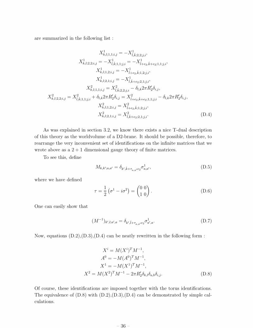
are summarized in the following list :

X1k,l;1,1;i,j = −X1

l,k;2,2;j,i,

X1k,l;2,2;i,j = −X1

l,k;1,1;j,i= −X1

l+e2,k+e2;1,1;j,i,

X1k,l;1,2;i,j = −X1

l+e2,k;1,2;j,i,

X1k,l;2,1;i,j = −X1

l,k+e2;2,1;j,i,

X2k,l;1,1;i,j = X2

l,k;2,2;j,i− δl,k2πR

′2δi,j ,

X2k,l;2,2;i,j = X2

l,k;1,1;j,i+ δl,k2πR

′2δi,j = X2

l+e2,k+e2;1,1;j,i− δl,k2πR

′2δi,j ,

X2k,l;1,2;i,j = X2

l+e2,k;1,2;j,i,

X2k,l;2,1;i,j = X2

l,k+e2;2,1;j,i. (D.4)

As was explained in section 3.2, we know there exists a nice T-dual description

of this theory as the worldvolume of a D2-brane. It should be possible, therefore, to

rearrange the very inconvenient set of identifications on the infinite matrices that we

wrote above as a 2 + 1 dimensional gauge theory of finite matrices.

To see this, define

Mk,k′;a,a′ = δk′,k+τa,a′e2σ1

a,a′ , (D.5)

where we have defined

τ =1

2

(σ1 − iσ2

)=

(0 0

1 0

). (D.6)

One can easily show that

(M−1)k′,l;a′,a = δk′,l+τa,a′e2σ1

a′,a. (D.7)

Now, equations (D.2),(D.3),(D.4) can be neatly rewritten in the following form :

X i = M(X i)TM−1,

A0 = −M(A0)TM−1,

X1 = −M(X1)TM−1,

X2 = M(X2)TM−1 − 2πR′2δk,lδa,bδi,j. (D.8)

Of course, these identifications are imposed together with the torus identifications.

The equivalence of (D.8) with (D.2),(D.3),(D.4) can be demonstrated by simple cal-

culations.

– 36 –

Next, we rearrange the fields as Fourier components in the k,l indices :

A0a,b;i,j(x, t) =

∑

k

(A0)0,k;a,b;i,jei“

k1x1R1

+k2x2R2

”

,

A1a,b;i,j(x, t) =

∑

k

X10,k;a,b;i,je

i“

k1x1R1

+k2x2R2

”

,

A2a,b;i,j(x, t) =

∑

k

X20,k;a,b;i,je

i“

k1x1R1

+k2x2R2

”

,

∀l = 3...9 X la,b;i,j(x, t) =

∑

k

X l0,k;a,b;i,je

i“

k1x1R1

+k2x2R2

”

, (D.9)

where R1 ≡ l2s/R′1 and R2 ≡ l2s/2R

′2 . The Lagrangian governing these fields is given

by a maximally supersymmetric (after including the fermions) Yang-Mills theory in

2 + 1 dimensions (16 real supercharges), which is the dimensional reduction of the

ten dimensional N = 1 SYM theory. However, there are some inter-relations among

the fields which we now derive. For convenience we suppress the i, j indices. The

inter-relations comprise the following set of additional relations on the theory with

16 supercharges (j = 3, · · · , 9) :

Xj1,1(x, t) = (Xj

2,2(−x, t))T ,

Xj1,2(x, t) = e

−ix2R2 (Xj

1,2(−x, t))T ,

Xj2,1(x, t) = e

ix2R2 (Xj

2,1(−x, t))T ,

A01,1(x, t) = −(A0

2,2(−x, t))T ,

A01,2(x, t) = −e−i

x2R2 (A0

1,2(−x, t))T ,

A02,1(x, t) = −ei

x2R2 (A0

2,1(−x, t))T ,

A11,1(x, t) = −(A1

2,2(−x, t))T ,

A11,2(x, t) = −e−i

x2R2 (A1

1,2(−x, t))T ,

A12,1(x, t) = −ei

x2R2 (A1

2,1(−x, t))T ,

A21,1(x, t) = (A2

2,2(−x, t))T − 2πR′2δi,j ,

A21,2(x, t) = e

−ix2R2 (A2

1,2(−x, t))T ,

A22,1(x, t) = e

ix2R2 (A2

2,1(−x, t))T .

(D.10)

We see that our theory can be written on a cylinder of volume (2πR1) × (πR2)

with orientifold planes at the boundaries. We can read the relevant boundary con-

ditions from (D.10). As the action appears to be an orbifold of the maximally

supersymmetric action we write it explicitly :

S =1

2g2YM

∫

T2

dtd2xTr

(−1

2FµνF

µν + (DµXj)2 +

1

2[Xj, X i][Xj , X i] + fermions

).

(D.11)

– 37 –

The size of T2 is (2πR1) × (2πR2). All the fields are periodic and in our case take

the form

X =

(X1,1;i,j X1,2;i,j

X2,1;i,j X2,2;i,j

), A =

(A1,1;i,j A1,2;i,j

A2,1;i,j A2,2;i,j

), i, j = 1, · · · , N.

(D.12)

We split the action :

S =1

2g2YM

∫dt

∫ 2πR1

0

dx1

∫ 0

−πR2

dx2 Tr

(−1

2FµνF

µν + (DµXj)2 +

1

2[Xj, X i][Xj , X i]

)+

+1

2g2YM

∫dt

∫ 2πR1

0

dx1

∫ πR2

0

dx2 Tr

(−1

2FµνF

µν + (DµXj)2 +

1

2[Xj , X i][Xj, X i]

)

(D.13)

Using (D.10) we can reexpress all the fields in the domain [−πR2, 0] as fields in

the domain [0, πR2]. The computation becomes very easy if one notices that the set

of equations (D.10) is actually simple, ∀j = 3, · · · , 9 :

Xj(x, t) = e− ix2

2R2σ3

σ1(Xj(−x, t))Tσ1eix2

2R2σ3

,

A0(1)(x, t) = −e−ix2

2R2σ3

σ1(A0(1)(−x, t))Tσ1eix2

2R2σ3

,

A2(x, t) = e− ix2

2R2σ3

σ1(A2(−x, t))Tσ1eix2

2R2σ3 − 2πR′

2σ3, (D.14)

where the relations are on the full 2N×2N matrices. The sigma matrices are always

tensored with the unit matrix of dimension N × N . One can see that this gives a

nice Lagrangian, as most of the commutators are invariant, or change sign. One easy

way to proceed is to rewrite the above lagrangian with new fields in the following

way :

Xj(x, t) = eix2σ3

4R2 Xj(x, t)e− ix2σ3

4R2 ,

A0(1)(x, t) = eix2σ3

4R2 A0(1)(x, t)e− ix2σ3

4R2 ,

A2(x, t) = eix2σ3

4R2 A2(x, t)e− ix2σ3

4R2 + σ3πR′2. (D.15)

This transformation is a U(2N) gauge transformation. Hence the Lagrangian of the

tilded fields is actually the same Lagrangian as (D.13). We will still name those fields

in the usual notation omitting the tildes. The identification of the tilded fields17 is

very suggestive:

Xj(x, t) = σ1(Xj(−x, t))Tσ1,

A0(1)(x, t) = −σ1(A0(1)(−x, t))Tσ1,

A2(x, t) = σ1(A2(−x, t))Tσ1. (D.16)

17As mentioned, we won’t use the notation of the tildes anymore.

– 38 –

Using this transformations we transform the [−πR2, 0] interval of the action to

[0, πR2], and we find that it precisely agrees with the original action for this in-

terval. The relative minus signs in the gauge fields exactly compensate for the minus

signs that arise because [AT , BT ] = −([A,B])T and because ∂2 → −∂2. So, our final

result is

S =1

2g2YM

∫dt

∫ 2πR1

0

dx1

∫ πR2

0

dx2 Tr(− 1

2FµνF

µν + (DµXj)2+

+1

2[Xj, X i][Xj , X i] + fermions

). (D.17)

We will determine gYM soon, so we omitted the factor 2 for now.18 The boundary

conditions are interesting. Equations (D.15) tell us that

Xj(x1, x2 + 2πR2, t) = σ3Xj(x1, x2, t)σ3,

A0,1,2(x1, x2 + 2πR2, t) = σ3A0,1,2(x1, x2, t)σ3. (D.18)

Combined with equations (D.16) we obtain

Xj(x1,−x2 + 2πR2, t) = σ2(Xj(x, t))Tσ2,

A0,1(x1,−x2 + 2πR2, t) = −σ2(A0,1(x1, x2, t))Tσ2,

A2(x1,−x2 + 2πR2, t) = σ2(A2(x1, x2, t))Tσ2. (D.19)

The boundary conditions at the two orientifold planes are, hence, different.19 For

x2 = 0 the matrices satisfy

Xj = σ1(Xj)Tσ1, ∂2Xj = −σ1(∂2X

j)Tσ1, (D.20)

A0(1) = −σ1(A0(1))Tσ1, ∂2A0(1) = σ1(∂2A

0(1))Tσ1, (D.21)

A2 = σ1(A2)Tσ1, ∂2A2 = −σ1(∂2A

2)Tσ1, (D.22)

so they are of the form

A2 , Xj =

(N S

S NT

)N+ = N, ST = S, ST = S, S+ = S,

A0 , A1 =

(M R

R −MT

)M+ = M, RT = −R, RT = −R, R+ = R. (D.23)

Collecting all these facts together we get that the gauge group in the bulk is

U(2N) while on the x2 = 0 boundary the gauge group is SO(2N). On this boundary

the fields A2, Xj are in the symmetric representation of the gauge group.

18The Lagrangian (D.17) on the cylinder defines what we mean by gYM so there is no ambiguity.19These are the anticipated O− and O+ planes.

– 39 –

The second boundary x2 = πR2 is substantially different. We write the boundary

conditions there in a familiar form

σ2Xjσ2 = (Xj)T , σ2∂2Xjσ2 = −(∂2X

j)T , (D.24)

σ2A0,1σ2 = −(A0,1)T , σ2∂2A0,1σ2 = (∂2A

0,1)T , (D.25)

σ2A2(x1, t)σ2 = (A2(x1, t))T , σ2∂2A2σ2 = −(∂2A

2)T . (D.26)

Consequently, the gauge group at this boundary is USp(2N). The most general

matrices are of the form

A2 , Xj =

(N S

S NT

)N+ = N, ST = −S, ST = −S, S+ = S,

A0 , A1 =

(M R

R −MT

)M+ = M, RT = R, RT = R, R+ = R. (D.27)

It is easy to verify that this precisely agrees with the action and boundary condi-

tions that we wrote down in the main text for the D2-brane between two orientifold

planes, if we only include the disk contributions to this action and not the Mobius

strip contributions.

References

[1] J. de Boer, R. Dijkgraaf, K. Hori, A. Keurentjes, J. Morgan, D. R. Morrison, and

S. Sethi, Triples, fluxes, and strings, Adv. Theor. Math. Phys. 4 (2002) 995–1186,

[hep-th/0103170].

[2] A. Keurentjes. Private communication.

[3] D. Kabat and S. J. Rey, Wilson lines and T-duality in heterotic M(atrix) theory,

Nucl. Phys. B508 (1997) 535–568, [hep-th/9707099].

[4] P. Horava and E. Witten, Heterotic and type I string dynamics from eleven

dimensions, Nucl. Phys. B460 (1996) 506–524, [hep-th/9510209].

[5] J. Polchinski and E. Witten, Evidence for heterotic - type I string duality, Nucl.

Phys. B460 (1996) 525–540, [hep-th/9510169].

[6] J. Dai, R. G. Leigh, and J. Polchinski, New connections between string theories, Mod.

Phys. Lett. A4 (1989) 2073–2083.

[7] D. R. Morrison and N. Seiberg, Extremal transitions and five-dimensional

supersymmetric field theories, Nucl. Phys. B483 (1997) 229–247, [hep-th/9609070].

[8] O. Bergman, M. R. Gaberdiel, and G. Lifschytz, String creation and heterotic-type I’

duality, Nucl. Phys. B524 (1998) 524–544, [hep-th/9711098].

– 40 –

[9] C. P. Bachas, M. B. Green, and A. Schwimmer, (8,0) quantum mechanics and

symmetry enhancement in type I’ superstrings, JHEP 01 (1998) 006,

[hep-th/9712086].

[10] A. Dabholkar and J. Park, Strings on orientifolds, Nucl. Phys. B477 (1996)

701–714, [hep-th/9604178].

[11] A. Keurentjes, Orientifolds and twisted boundary conditions, Nucl. Phys. B589

(2000) 440–460, [hep-th/0004073].

[12] M. Gutperle, Non-BPS D-branes and enhanced symmetry in an asymmetric orbifold,

JHEP 08 (2000) 036, [hep-th/0007126].

[13] S. Hellerman, New type II string theories with sixteen supercharges, hep-th/0512045.

[14] C. Vafa and E. Witten, Dual string pairs with N=1 and N=2 supersymmetry in four

dimensions, Nucl. Phys. Proc. Suppl. 46 (1996) 225–247, [hep-th/9507050].

[15] E. Witten, Toroidal compactification without vector structure, JHEP 02 (1998) 006,

[hep-th/9712028].

[16] A. Keurentjes, Discrete moduli for type I compactifications, Phys. Rev. D65 (2002)

026007, [hep-th/0105101].

[17] A. Sen, F-theory and orientifolds, Nucl. Phys. B475 (1996) 562–578,

[hep-th/9605150].

[18] S. Chaudhuri, G. Hockney, and J. D. Lykken, Maximally supersymmetric string

theories in D¡10, Phys. Rev. Lett. 75 (1995) 2264–2267, [hep-th/9505054].

[19] S. Chaudhuri and J. Polchinski, Moduli space of CHL strings, Phys. Rev. D52

(1995) 7168–7173, [hep-th/9506048].

[20] J. Park, Orientifold and F-theory duals of CHL strings, Phys. Lett. B418 (1998)

91–97, [hep-th/9611119].

[21] A. Mikhailov, Momentum lattice for CHL string, Nucl. Phys. B534 (1998) 612–652,

[hep-th/9806030].

[22] T. Banks, W. Fischler, S. H. Shenker, and L. Susskind, M theory as a matrix model:

A conjecture, Phys. Rev. D55 (1997) 5112–5128, [hep-th/9610043].

[23] L. Susskind, Another conjecture about m(atrix) theory, hep-th/9704080.

[24] N. Seiberg, Why is the matrix model correct?, Phys. Rev. Lett. 79 (1997) 3577–3580,

[hep-th/9710009].

[25] A. Sen, D0 branes on T n and matrix theory, Adv. Theor. Math. Phys. 2 (1998)

51–59, [hep-th/9709220].

– 41 –

[26] A. Keurentjes, Determining the dual, hep-th/0607069.

[27] T. Banks, N. Seiberg, and E. Silverstein, Zero and one-dimensional probes with N=8

supersymmetry, Phys. Lett. B401 (1997) 30–37, [hep-th/9703052].

[28] T. Banks and L. Motl, Heterotic strings from matrices, JHEP 12 (1997) 004,

[hep-th/9703218].

[29] D. A. Lowe, Heterotic matrix string theory, Phys. Lett. B403 (1997) 243–249,

[hep-th/9704041].

[30] S.-J. Rey, Heterotic M(atrix) strings and their interactions, Nucl. Phys. B502 (1997)

170–190, [hep-th/9704158].

[31] P. Horava, Matrix theory and heterotic strings on tori, Nucl. Phys. B505 (1997)

84–108, [hep-th/9705055].

[32] N. Kim and S.-J. Rey, Non-orientable M(atrix) theory, hep-th/9710192.

[33] N. Kim and S. J. Rey, M(atrix) theory on an orbifold and twisted membrane, Nucl.

Phys. B504 (1997) 189–213, [hep-th/9701139].

[34] G. Zwart, Matrix theory on non-orientable surfaces, Phys. Lett. B429 (1998) 27–34,

[hep-th/9710057].

[35] O. Bergman, E. G. Gimon, and P. Horava, Brane transfer operations and t-duality of

non-bps states, JHEP 04 (1999) 010, [hep-th/9902160].

[36] W. Taylor, D-brane field theory on compact spaces, Phys. Lett. B394 (1997)

283–287, [hep-th/9611042].

[37] L. Motl, Proposals on nonperturbative superstring interactions, hep-th/9701025.

[38] T. Banks and N. Seiberg, Strings from matrices, Nucl. Phys. B497 (1997) 41–55,

[hep-th/9702187].

[39] R. Dijkgraaf, E. P. Verlinde, and H. L. Verlinde, Matrix string theory, Nucl. Phys.

B500 (1997) 43–61, [hep-th/9703030].

[40] W. Fischler, E. Halyo, A. Rajaraman, and L. Susskind, The incredible shrinking

torus, Nucl. Phys. B501 (1997) 409–426, [hep-th/9703102].

[41] S. Govindarajan, Heterotic M(atrix) theory at generic points in Narain moduli space,

Nucl. Phys. B507 (1997) 589–608, [hep-th/9707164].

[42] F. A. Cachazo and C. Vafa, Type I’ and real algebraic geometry, hep-th/0001029.

[43] O. J. Ganor, S. Ramgoolam, and W. Taylor, Branes, fluxes and duality in

M(atrix)-theory, Nucl. Phys. B492 (1997) 191–204, [hep-th/9611202].

[44] O. Aharony, Z. Komargodski and A. Patir, work in progress.

– 42 –

[45] A. Hanany and B. Kol, On orientifolds, discrete torsion, branes and M theory, JHEP

06 (2000) 013, [hep-th/0003025].

[46] P. M. Ho, Y. Y. Wu, and Y. S. Wu, Towards a noncommutative geometric approach

to matrix compactification, Phys. Rev. D58 (1998) 026006, [hep-th/9712201].

– 43 –