arX

iv:h

ep-t

h/99

1018

1v2

24

Oct

199

9

M-Theory, Topological Strings and

Spinning Black Holes

Sheldon Katz, Albrecht Klemm and Cumrun Vafa

Department of Mathematics, Oklahoma State University, Stillwater, OK 74078, USA

Institute for Advanced Study, Princeton, NJ 08540, USA

Jefferson Laboratory of Physics, Harvard University, Cambridge, MA 02138, USA

Abstract

We consider M-theory compactification on Calabi-Yau threefolds. The recently dis-

covered connection between the BPS states of wrapped M2 branes and the topological

string amplitudes on the threefold is used both as a tool to compute topological string

amplitudes at higher genera as well as to unravel the degeneracies and quantum numbers

of BPS states. Moduli spaces of k-fold symmetric products of the wrapped M2 brane play

a crucial role. We also show that the topological string partition function is the Calabi-Yau

version of the elliptic genus of the symmetric product of K3’s and use the macroscopic en-

tropy of spinning black holes in 5 dimensions to obtain new predictions for the asymptotic

growth of the topological string amplitudes at high genera.

HUTP-99/A056, IASSNS-HEP-98/107, OSU-M-99-9

email: katz@math.okstate.edu, klemm@ias.edu, vafa@string.harvard.edu

Table of Contents

1. Introduction

2. Topological Strings (A-model)

2.1 The genus 0 contribution

2.2 The genus 1 contribution

2.3 The constant map contribution

3. M-theory/Type IIA interpretation of the Fr

3.1 The new invariants

3.2 The higher genus contributions

4. Computation of nrd

4.1 Computational scheme for nrd

5. Considerations of Enumerative Geometry

5.1 Alternative interpretation of the nrd

6. Application to counting M2 branes in K3 × T 2

6.1 Zero winding on the T 2

6.2 More general H2 classes in K3 × T 2

7. Black Hole Entropy and Topological String

8. Computations in local Calabi-Yau geometries

8.1 Basic concepts

8.2 O(−1) ⊕O(−1) → P1

8.3 Local P2: O(−3) → P2

8.4 Local P1 ×P1: O(K) → P1 ×P1

8.5 Other local Del Pezzo geometries E5, E6, E7 and E8

8.6 The topological string perspective

1

Table of Contents (continued)

9. Computations in compact Calabi-Yau geometries

9.1 Compact one modulus cases

9.2 Higher genus results on the quintic

9.3 The sextic, the bicubic and four conics

10. Appendix A: Low degree classes on the del Pezzo Surfaces

11. Appendix B: B-model expression for Fg

2

1. Introduction

The study of Calabi-Yau threefolds has been a source of many new ideas in string

theory. Not only they are useful as building blocks of various string compactifications, but

they also provide interesting examples of exactly computable quantities in string theory. In

particular they correspond to the “critical dimension” for the (N = 2) topological string.

Topological strings, roughly speeking, count the number of holomorphic curves inside

the Calabi-Yau. As such, one would expect that they should correspond to the partition

function of M2 (or D2)-branes wrapped around them. The connection at first sight seems

somewhat confusing: The topological string amplitudes exist for each genus, whereas the

M2 brane (or D2 brane) degeneracies only care about the charge and not the genus of the

curve representing it. It turns out, as discovered in [1], that the genus dependence of the

topological string amplitudes captures the SU(2)L representation content of BPS states

corresponding to wrapped M2 branes upon compactifications of M-theory on Calabi-Yau

threefolds. Here SU(2)L denotes a subgroup of the SO(4) rotation group in 5 dimensions.

This identification was based on the target space interpretation of what the topological

string computes [2][3] and the contribution of BPS states to such terms (using a Schwinger

1-loop computation) [4].

Topological string amplitudes at genus 0 can be computed using mirror symmetry

[5]. For higher genera, mirror symmetry is still a powerfull principle and can be used to

compute the amplitudes up to a finite number of undetermined constants at each genus

[2]. Fixing the constant is called fixing the ‘holomorphic ambiguity’, and for the certain

cases they were fixed for genus 1 and genus 2 in [6][2]. The number of unknown constants

grows with the genus. In certain cases one can use direct A-model localization [7] to fix

these constants and in particular checking the integrality properties of topological string

partition functions, anticipated in [1], at higher g ≤ 5.

In this paper we wish to use the reformulation of topological string amplitudes as a

computation of BPS states in M-theory compactifications [1] to make progress in explicit

computations of topological strings at higher genera. The reorganization this introduces

into topological string amplitudes is to fix the BPS charge and consider all allowed genera of

the M2 brane at the same time. For a given degree, there typically is a highest genus curve

embedded in the 3-fold which realizes that class1 . One then studies the moduli space

1 This highest genus is the arithmetic genus which we will often denote by g. The topological

string amplitude at genus g usually denoted Fg has contributions from curves of different arith-

metic genera. If the distinction is important we use the label r to refer to the worldsheet genus

and write Fr etc.

3

of that curve, together with the flat bundle over it. Understanding of the cohomology

of this moduli space and the SU(2)L action on it, will in particular determine the BPS

degeneracy and its SU(2)L quantum numbers. This in particular affects the topological

string amplitudes for all Fr with r ≤ g in a well defined way. The main aim of our paper

is to develop techniques that at least in some cases allows us to extract from the geometry

of this moduli space the SU(2)L action on its cohomology. We relate the degeneracies for

a fixed SU(2)L spin, and in particular its contribution to Fr, to the Euler characteristic of

the δ = g − r fold symmetric product of the holomorphic curves in the Calabi-Yau 3-fold

and to higher Fk’s (r < k ≤ g). For δ sufficiently small this space is smooth and its Euler

characteristic can be computed. For δ too big, in general this space is not smooth and the

computation of its Euler characteristic requires more care. We will consider examples of

both types. We also use these results to fix the holomorphic ambiguities for higher genera

in some examples (and in particular we push up the computation of topological strings to

higher genera).

We will also discuss the connection of topological string amplitudes and the entropy

of spinning black holes corresponding to M2 branes wrapped over “large” cycles in the

Calabi-Yau. In particular we see how in the case of K3 × T 2 the elliptic genus of the

symmetric product of K3’s predicts complete answers to the SU(2)L action on the moduli

spaces that we study. For a general Calabi-Yau threefold, we see how the black hole entropy

predicts new growth properties for the topological string amplitudes at higher genera that

would be interesting to verify.

The organization of this paper is as follows: In section 2 we review the definition and

some results related to A-model topological strings. In section 3 we review the definition of

some of the new invariants which allows one to rewrite topological string amplitudes using

integral data. In section 4 we show how the new invariants can be effectively computed

in certain cases. In section 5 we show that the same invariants can also be computed in

a different way and be given a related geometric interpretation. In section 6 we show in

the case of K3×T 2 how the elliptic genus of symmetric products of K3 captures the BPS

degeneracies of a wrapped M2 brane and show how our methods can predict some of these

results. In section 7 we use predictions of macroscopic entropy of black holes to estimate

the growth of topological string amplitudes for high genera. In section 8 we give some

examples involving non-compact Calabi-Yau 3-folds and show how our methods work in

those cases. In section 9 we do the same, but in the context of compact CY 3-folds. In

appendix A we discuss some aspects of del Pezzo surfaces and in appendix B we discuss

some aspects of B-model topological strings.

4

2. Topological Strings (A-model)

In topological string theory (A-model) one considers maps from a Riemann surface

Σg of genus g to a manifold which in the case of interest in this paper we take to be a

Calabi-Yau threefold X . The partition function depends only on the complexified Kahler

moduli of X denoted by (ti, ti). In the limit whereby one fixes ti and takes the limit

ti → ∞, a holomorphic anomaly decouples, and the theory becomes purely topological. In

particular, in this limit the Fg(ti) are obtained by considering holomorphic maps from the

Riemann surface to X . Roughly speaking one has

Fg(ti) =∑

hol.mapf :Σg→X

exp(−∫

Σg

f∗(k))

where k is the Kahler class on X and f∗(k) is its pullback to Σ. The above formula is

not quite general because often holomorphic maps come in families. In these cases the

sum is replaced by an integral over the moduli space of holomorphic maps representing

some top characteristic class on the moduli space. More precisely, in the special case of

Calabi-Yau threefolds that we are considering the formal dimension of the moduli space

of maps is zero and when there is a moduli space of maps there is an equal dimensional

space corresponding to a cokernel of a bundle map. Thus the cokernel vector space forms

a bundle on the moduli space of curves whose Euler class enters the relevant topological

computation which enters in the above formula (for a more precise mathematical definition

and a review of the subject see [5]).2 The result of such integrals for each fixed topological

class of the image curve in X is known as the Gromov-Witten invariants. In other words

one can write

Fg(ti) =∑

di

fg,dexp(−diti)

where di denotes the homology class of the image curve in terms of some basis for H2(X,Z)

and fg,d are the Gromov-Witten invariants. Since in most cases of interest the computation

of fg,n involves integrals over moduli spaces, there is a priori no reason for them to be

integers, as they are not “counting” the number of holomorphic curves. However some

surprising integrality properties have already been observed for small genus which we

will review below. From the viewpoint of the topological string this integrality is very

2 Strictly speaking, the obstruction spaces need not form a bundle, and there can be a virtual

fundamental class in place of an Euler class.

5

surprising and has not been explained. An explanation of the observed integrality and

its generalization to all genera has been found in [1] based on M-theory/type IIA duality

which recasts Gromov-Witten invariants in terms of some new integral invariants nrd. In

this section we first review some aspects of topological strings. We then review the results

of [1] in section 3.

2.1. The genus 0 contribution

Let Lir(x) =∑∞k=1 k

−rxk, i.e. Li−r(x) = −(x d

dx

)rlog(1 − x) and Lir(x) =

−(∫

dxx

)rlog(1 − x) then [8] gives a formal expansion

F0 =K0t

3

3!+ t

∫

X

c2J +χ

2ζ(3) +

∞∑

d=1

n0d Li3(q

d) . (2.1)

Here K0 is the classical triple intersection number on X , which comes from the degree zero

maps.

The curve counting function in genus zero is Kttt = (∂t)3F0 = K0 +

∑∞d=1Kdq

d. By

(2.1), Kd is related to the n0d by

Kd =∑

n|d

n0d/n

n3. (2.2)

It was observed that in this way of writing the Gromov-Witten invariants the n0d are

integers [8] for the case of the quintic in P4 at least for degrees up to 300. This was

later extended to all d which are not multiples of 5. 3 An explanation of this integrality

was suggested in [8] as counting the “number of rational holomorphic curves” in Calabi-

Yau space. This was further supported by the fact that it was shown in [9] that the n

fold covering of an isolated holomorphic curve of degree d gives a contribution of 1/n3

to the Gromov-Witten invariant for degree dn in perfect accord with (2.2). However the

interpretation of n0d as counting holomorphic rational curves in X is in general not the

right interpretation. In particular a counter-example occurs even for isolated curves in the

quintic. In [10] a contribution of n05, nod = 17, 601, 000 plane curves with six nodes to total

number of curves at degree five n05 = 229, 305, 888, 887, 625 was found. There are three

contributions to K10: degree 10 curves, double covers of degree 5 curves, and additional

integer contributions for double covers of the 6-nodal curves corresponding to double covers

3 Lian and Yau also proved integrality of the coefficients of the mirror map for the quintic, and

in all the applications to toric hypersurfaces no non-integer n0d ever appeared.

6

with 2 components. Correspondingly for each double covering of a nodal curve there is

a higher dimensional stratum and six points in M0,0(X, 10) [5]. The contribution of

the higher dimensional strata to the degree 10 curves must therefore be calculated by a

virtual fundamental class calculation, which yields the usual 123 and so the double covering

contribution is 123 ·n0

5 smooth for the smooth d = 5 curves but (6+ 123 ) ·n0

5 nod for the nodal

ones. That means that the number4 of degree 10 curves on the quintic is not given by n010,

but rather by N10 = K10 − n01

1000 − n02

125 − n05

8 − 6n05, nod, see Example 7.4.4.1 and Theorem

9.2.6 in [5]. In particular n010 as defined in (2.2) has no interpretation as a “number” of

curves, and there is currently no known mathematical reason to expect it to be integer!

One aim of this paper is to outline a physically motivated geometrical definition of the nrd,

which makes the integrality manifest.

More generally, let C ⊂ X be a sufficiently general smooth curve of genus g satisfying

appropriate genericity hypotheses. Then Cg(h, d) denotes the contribution to Fg+h of

maps whose image is C whose image has class d[C]. It is not yet clear if this notion is

well-defined for g ≥ 2.

Extending [9] Faber and Pandharipande [11] prove that the multicover contribution

C0(h, d) of a P1 is described by

C0(g, d) = χgd2g−3 =

|B2g|d2g−3

2g(2g − 2)!with χ0 = 1, χ1 =

1

12. (2.3)

Here χ(Mg) =|B2g|

2g(2g−2)! is the Harer-Zagier formula for the orbifold Euler characteristic

of Mg in complete accordance with the predictions of M-theory [1] which will be discussed

later.

2.2. The genus 1 contribution

For r = 1 the situation is more interesting. The localization [11] gives

C1(0, d) =σ1(d)

d, C1(h, d) = 0 (h > 0). (2.4)

There is no bubbling contributions of genus 1 curves to higher genus curves, i.e.C1(h, d) = 0

for h > 0 in accordance with the above and the zero-mode analysis in [6]. This is a feature

one finds in the M-theory approach discussed in the next section.

4 We assume that there are finitely many curves (Clemens’ Conjecture). N10 could still contain

multiplicity factors for certain curves.

7

However the form of F1 discussed in the next section (which is most natural from the

M-theory perspective) is (up to the t-terms)

F1 =t∫c2J

24+

∞∑

d=1

(1

12n0d + n1

d

)Li1(q

d) . (2.5)

Here, n1d is an invariant of certain BPS states typically associated to wrapping M2 branes

around degree d elliptic curves E. This differs from the geometric substraction scheme

(2.4), as it does not subtract all the multicovering maps from the torus to itself in the

definition of the n1d, but instead subtracts 1/d for the class d[E]. Substraction of these

would yield5 [6]

F1 =t∫c2J

24+

∞∑

d=1

(1

12n0dLi1(q

d) + n∗1d log η(qd)

)(2.6)

where n∗1d corresponds to elliptic curves rather than BPS states. The reason for adding

back in the multicover contributions is discussed from the BPS perspective in the next

section.

Comparing (2.5) with (2.6)

∑

d,n

n1d

nqdn =

∑

d,n

n∗1d

σ1(n)

nqnd

and keeping in mind the definition σ1(n)n =

∑k|n

1k , we see that the number of BPS states

of charge d[E] is n1d =

∑m|d n

∗1m as expected from adding up all bound states.

2.3. The constant map contribution

We can compute for arbitrary genus in the simple case when the holomorphic maps

from the Riemann surface to X are just the constant maps. This is already a case where

there is a moduli space of such maps. If the degree of the map f is 0 its moduli space

splits into

Mg,n(X, 0) ∼ Mg,n ×X (2.7)

where Mg,n in this case corresponds to moduli space of genus g domain curves. The

relevant Gromov-Witten invariant in this case is given by 12e(X)

∫Mg

c3g−1(H) [2] where

e(X) denotes the Euler characteristic of X and H denotes the Hodge bundle (coming from

5 The genus zero contribution follows from (2.3) in both cases.

8

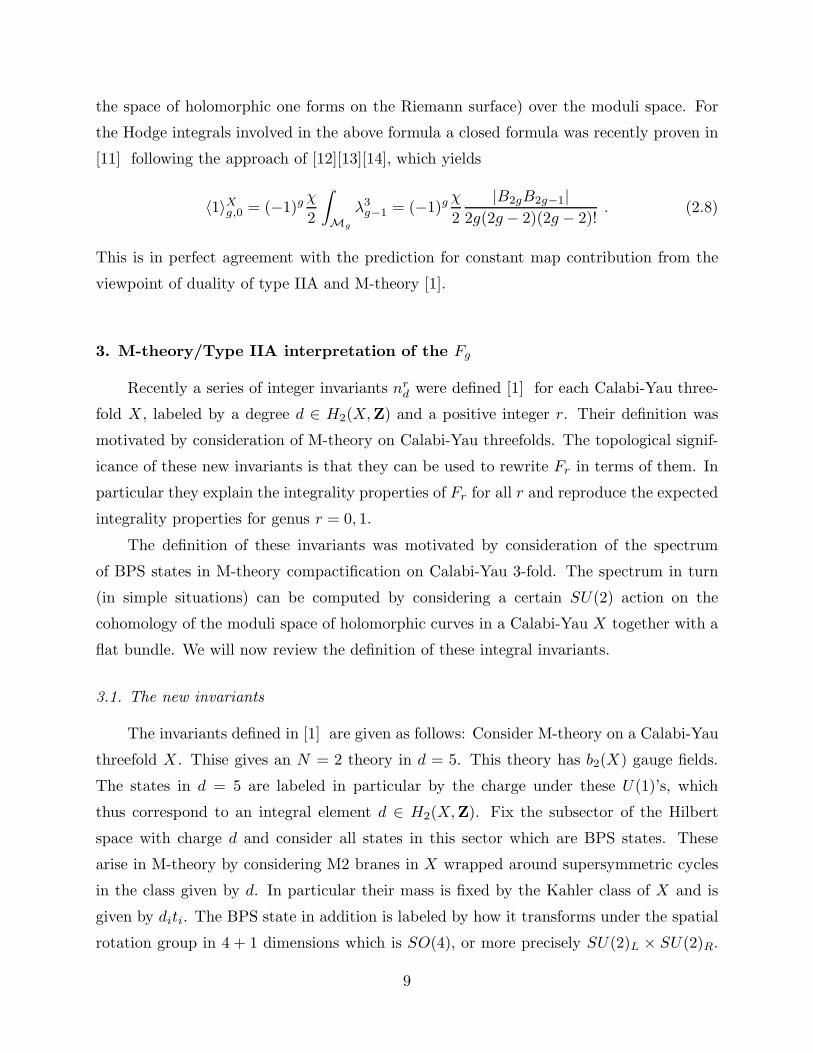
the space of holomorphic one forms on the Riemann surface) over the moduli space. For

the Hodge integrals involved in the above formula a closed formula was recently proven in

[11] following the approach of [12][13][14], which yields

〈1〉Xg,0 = (−1)gχ

2

∫

Mg

λ3g−1 = (−1)g

χ

2

|B2gB2g−1|2g(2g − 2)(2g − 2)!

. (2.8)

This is in perfect agreement with the prediction for constant map contribution from the

viewpoint of duality of type IIA and M-theory [1].

3. M-theory/Type IIA interpretation of the Fg

Recently a series of integer invariants nrd were defined [1] for each Calabi-Yau three-

fold X , labeled by a degree d ∈ H2(X,Z) and a positive integer r. Their definition was

motivated by consideration of M-theory on Calabi-Yau threefolds. The topological signif-

icance of these new invariants is that they can be used to rewrite Fr in terms of them. In

particular they explain the integrality properties of Fr for all r and reproduce the expected

integrality properties for genus r = 0, 1.

The definition of these invariants was motivated by consideration of the spectrum

of BPS states in M-theory compactification on Calabi-Yau 3-fold. The spectrum in turn

(in simple situations) can be computed by considering a certain SU(2) action on the

cohomology of the moduli space of holomorphic curves in a Calabi-Yau X together with a

flat bundle. We will now review the definition of these integral invariants.

3.1. The new invariants

The invariants defined in [1] are given as follows: Consider M-theory on a Calabi-Yau

threefold X . Thise gives an N = 2 theory in d = 5. This theory has b2(X) gauge fields.

The states in d = 5 are labeled in particular by the charge under these U(1)’s, which

thus correspond to an integral element d ∈ H2(X,Z). Fix the subsector of the Hilbert

space with charge d and consider all states in this sector which are BPS states. These

arise in M-theory by considering M2 branes in X wrapped around supersymmetric cycles

in the class given by d. In particular their mass is fixed by the Kahler class of X and is

given by diti. The BPS state in addition is labeled by how it transforms under the spatial

rotation group in 4 + 1 dimensions which is SO(4), or more precisely SU(2)L × SU(2)R.

9

In particular we can write the degeneracy of the BPS states together with their SO(4)

quantum numbers as

[(1

2, 0

)⊕ 2(0, 0)

]⊗⊕

jL,jR

NdjL,jR

[(jL, jR)]. (3.1)

The numbers NdjL,jR

denote the number of BPS states with charge represented by the class

d and with SU(2)L × SU(2)R representation given by the rerpresentation (jL, jR), where

jL, jR ∈ (1/2)Z and denote the spin of the representations.

The number of BPS states is not an invariant of the theory and it can jump. Two

(short) BPS multiplets can join and become a (long) non BPS multiplet. For example,

changing the complex structure of the Calabi-Yau X will change the numbers NdjL,jR

.

However, the left index of the representation does not change. In other words, if we

consider the degeneracies with respect to SU(2)L and sum over all SU(2)R quantum

numbers multiplied by (−1)2jR = (−1)FR , then this weighted sum of left representations

does not change. 6 It is more useful for comparison with topological strings to choose a

different basis for the SU(2)L representations. Let

Ir = [(1

2) + 2(0)]⊗r.

Using this basis, the procedure is

NdjL,jR [(jL, jR)] →

∑NdjL,jR(−1)2jR(2jR + 1)[(jL)] =

∑

r

nrdIr (3.2)

The above equation defines the invariants nrd which appear in the partition function of the

topological string. According to [1] we have:

F =∞∑

r=0

λ2r−2Fr =∞∑

r=0

∑

d=0m=1

nrd1

m

(2 sin

mλ

2

)2r−2

qdm. (3.3)

6 There are well known examples, e.g. [15], where the individual right spin content changes

under complex structure deformation. Consider a P1 fibered over a genus g curve Cg. The right

Leshetz decomposition of the base M = Cg is[

12

]+ 2g[0]. Vanishing complex volume of the P

1

corresponds to a special value on the Coulomb branch φ = 0 with a SU(2) gauge enhancement

and g hypermultiplets in the adjoint representation. Higgsing w.r.t. to the diagonal components

of the hypers corresponds to a complex structure deformation and breaks the gauge group to U(1)

and 2g− 2 charged hypers, which geometrically corresponds to a splitting of the P1 fibration into

2g − 2 isolated P1’s, whose right spin content is (2g − 2)[0].

10

The argument leading to this identification is that the topological string can be viewed as

computing∑FrR

2+F

2r−2+ λ2r−2 amplitudes in four dimensions upon considering type IIA

compactification on the Calabi-Yau. Here R+ and F+ denote self-dual parts of the Rie-

mann tensor and graviphoton field strength, respectively [2][3]. Then a 1-loop Schwinger

computation as in [4] with the BPS states running around the loop relates the BPS content

of states in 5-dimensional M-theory to corrections to R2+F

2r−2+ amplitudes. The appear-

ance of the extra sum over m in (3.3) is related to the momentum a BPS state in 5

dimensions can have when compactified on a circle down to 4 dimensions. These appear

as ‘multi-cover’ contributions in the topological string context, as first noticed for the case

of genus 0 by [16]. The term (2 sin mλ2

)2r in the above formula arises from computation of

Tr(−1)2jL+2jR exp(2imλJ3L) in the Ir representation, where J3

L is one of the generators of

SU(2)L.

3.2. The higher genus contributions

Expanding (3.3) gives back (2.1), i.e. the naive multicovering formula (2.2) for the

rational curves, which first was empirically observed in [8]. Of course the physical picture

relates the integers nrd naturally to the number of BPS states. Note also that with the ζ-

function renormalization one gets the well known [8] subleading contribution to the genus

zero pre-potential χ(X)ζ(3)/2 from (2.7)(3.3).

Using genus r = 0, 1 as a model, we can try to recursively define nrd by

Krd =

∑

k|dh≤r

nhkCh(r − h,d

k),

whereKrd are the Gromov-Witten invariants defined by Fr =

∑Krdqd. This is the approach

taken in [5] for r = 0, 1; there the numbers nrd are called instanton numbers (see [5] for a

precise version of the integrality conjecture for r = 0).

For the elliptic curve T 2 and any n, we can consider n D2 branes wrapped on T 2.

In this case as discussed in [1] to count the number of BPS states we should consider the

moduli space of stable rank n bundles on T 2. There are indecomposable (semi)stable U(n)

bundles over T 2, which corresponds to a BPS bound state of n D2 branes wrapping T 2

(the corresponding space for genus 0 is empty which is why we do not have bound states

of n D2 branes on a genus 0 curve). This explains the scheme used in the previous section

in defining the BPS numbers for genus 1.

11

For the genus 2,3 expansion we have

F2 =χ

5760+

∞∑

d=1

(1

240n0d + n2

d

)Li−1(q

d) (3.4)

F3 = − χ

1451520+

∞∑

d=1

(1

6048n0d −

1

12n2d + n3

d

)Li−3(q

d) (3.5)

and similarly for higher genus

Fr=(−1)rχ|B2rB2r−2|4r(2r − 2)!(2r − 2)

+∞∑

d=1

( |B2r|n0d

2r(2r− 2)!+

2(−1)rn2d

(2r − 2)!±. . .− r − 2

12nr−1d + nrd

)Li3−2r

(3.6)

There is a subtlety for genus r > 2 in that n D2 brane bound states can deform off the

supporting genus r curve. This is briefly discussed in [1] and is a topic for further study.

4. Computation of nrd

The identity (3.3) reexpresses topological string amplitudes in terms of integral quan-

tities nrd defined in terms of the BPS spectrum of M-theory on Calabi-Yau threefolds

according to (3.2). If one finds a simple way to compute the new invariants nrd this would

translate to a practical method of computing topological string amplitudes.

In [1] it was shown how one goes about computing nrd (at least in certain good cases).

The basic idea is to consider the moduli space of M2 branes, which gets translated using

M-theory/IIA duality to the study of certain aspects of moduli space of D2 branes. One

considers supersymmetric D2 branes whose class in X is given by [D2] = d. The moduli

space of such configurations is given, in addition to the embedding of the D2 brane, by

the choice of a flat bundle on the brane. In general if we have N coincident branes, we

will have to consider also the moduli of flat U(N) bundles in addition to the moduli of the

embeddings of the D2 branes. Let us consider the simple case where we have a single D2

brane in class d and let us denote by M the moduli space of holomorphic curves in X in

class d, together with the choice of the flat bundle on the Riemann surface. Let M denote

the moduli space of holomorphic curves in class d, without the choice of the flat bundle.

Then we have a map

M → M

Let us assume that generically the Riemann surface has genus g. Then the above map

has generically a fiber which is T 2g, i.e. the Jacobian of the Riemann surface. However

12

generally speaking there are loci where the genus g surface become singular. For example

it can develop nodes by having some pinched cycles. Similarly the Jacobian torus becomes

singular in this limit.7 Nevertheless, one expects the total space M to be smooth (similar

to description of elliptic fibration of K3 where the fibration becomes singular at 24 points,

but the K3 is smooth). Because of this smoothness, for many questions it is possible

to treat the above fibration as if there are no degenerate fibers. In particular, consider

the integral (1,1) form k corresponding to the fiber T 2g (usually denoted on each non-

degenerate fiber by k|fiber = θ = dz(ImΩ−1)dz∗). We will assume, as is the case with

smooth Jacobian varieties, that k makes sense as an integral (1,1) class in M.

Consider the cohomology of the manifold M. These will correspond to BPS states in

M-theory compactification. Moreover the SU(2)L quantum numbers get morally identified

with the SL(2) Lefschetz decomposition in the fiber direction (i.e. using k as a raising op-

erator) and the SU(2)R quantum numbers get morally identified with the SL(2) Lefschetz

decomposition in the base direction (i.e. using the Kahler form on the base). In other

words we have [1]:

H∗(M) =∑

Ndj1,j2

[jfiber1 , jbase2 ] (4.1)

from which we can read off nrd according to (3.2). There are precise statements that can

be made: the usual Lefschetz decomposition of the cohomology M is identified with the

diagonal SL(2) ⊂ SL(2)fiber × SL(2)base, and the SU(2)R content of the highest left spin

is identified with the Lefschetz decomposition of H∗(M).

There are two particularly easy cases to compute from the above definition, namely:

ngd = (−1)dimMe(M)

n0d = (−1)dimMe(M)

(4.2)

where e(...) denotes the Euler characteristic of the space. The relations follow from the

definition of what the double Lefschetz action is. As we will demonstrate in the next

section, the other non-vanishing n’s, i.e. the nrd for 0 < r < g can also be related to

particular combinations of Euler characteristics of certain subspaces in M. Sometimes we

will write r = g − δ where δ is a positive integer less than or equal to g.

The existence of such a double Lefschetz decomposition is expected from the M-theory

description of the BPS states in 5 dimensions and so it should be possible to rigorize the

existence of the above double SL(2) decomposition of the cohomology of M. However

7 More precisely, the compactified Jacobian becomes singular in this limit.

13

here we would like to get the new invariants with the minimal amount of assumptions

about the properties of M. As we will discuss in the next section all we really need for

computation of nrd is the existence of a smooth manifold M and an integral (1,1) class k

which on smooth fibers is the canonical (1, 1) class on the Jacobian torus. This will also

lead to a simple formulation for the computation of all nrd in terms of Euler characteristics

of relative Hilbert schemes, which are frequently easy to compute.

4.1. Computational Scheme for nrd

As is clear from (4.1) and (3.2) all we need to compute the nrd is the Lefschetz action

in the fiber direction. We will see that in fact we can compute nrd without this assumption

in a reasonably general setting.

For each point on the base M let C denote the corresponding Riemann surface and

J (C) its Jacobian. The Riemann surface together with the choice of p points on it, is

what is called the Hilbert scheme of p points on C, and denoted by Hilbp(C). We have

the Abel-Jacobi mapping [17]:

fp : Hilbp(C) → J (C) (4.3)

whose image is denoted by Wp. We can relate the cohomology of Wp to the cohomologies

of both Hilbp(C) and J (C), thereby relating these two cohomologies directly.

We have the map H∗(Wp) → H∗(J (C)), which by Poincare duality is identified with

a map i : H∗(Wp) → H∗(J (C)) whose image we wish to compute. Let θ ∈ H1,1(J (C)) be

the cohomology class of the zero locus of the theta function on J (C). Since the image Wp

of fp is dual to θg−p/(g − p)![17], the composition of the restriction map r : H∗(J (C)) →H∗(Wp) with i is (up to the constant which we ignore) just the multiplication map

θg−p : H∗(J (C)) → H∗(J (C)).

Since there is also a map f∗p : H∗(Wp) → H∗(Hilbp(C)), we expect to be able to relate

H∗(Hilbp(C)) with the image of θg−p.

Here is our strategy. Once we understand this relation, we consider varying the point

on the base M. In this way the Abel-Jacobi map fp gets promoted to a map

fp : C(p) → M. (4.4)

14

Here C(p) denotes the moduli space of holomorphic curves of degree d together with the

choice of p points on the Riemann surface.8 Therefore we relate H∗(Cp) to the image

of multiplication by kg−p on H∗(M), where k is the SU(2) raising operator in the fiber

direction. This can be used to compute ng−δd according to (4.1) and (3.2).

Before we carry this out, it is first convenient to review some facts about the coho-

mology of the Hilbert scheme of p points on the Riemann surface C. Let C be a smooth

curve of genus g. Then we have for its cohomology, as an SU(2) Lefschetz representation

H∗(C) = (1

2) ⊕ (2g)(0). (4.5)

For a smooth curve, its Hilbert scheme is the same as its symmetric product. Taking

symmetric products, we have for the Lefschetz SU(2) decomposition

H∗(Hilbk(C)) =⊕

r

Symr

(1

2

)⊗ ∧k−r(2g)(0)

=k⊕

r=0

(2g

k − r

)( r

2

) (4.6)

Note that since the 2g(0) represent odd cohomology of C, we must antisymmetrize.

For convenience, we explicitly list the first two cases of (4.6)

H∗(Hilb2(C)) = (1) ⊕ (2g)(1

2) ⊕ (2g2 − g)(0)

H∗(Hilb3(C)) = (3

2) ⊕ (2g)(1)⊕ (2g2 − g)(

1

2) ⊕ (

4

3g3 − 2g2 +

2

3g)(0).

(4.7)

The Jacobian J (C) is a principally polarized abelian variety [17], so as we have already

mentioned has a canonical Kahler class θ ∈ H1,1(J (C)), whose corresponding divisor is the

zero locus of the theta-function on J (C). It is straightforward to check that the resulting

Lefschetz SU(2) representation content of H∗(J (C)) can be identified with Ig, which is

the representation we defined before. Furthermore, the class θ in this context is identified

with the SU(2) raising operator k. So θg−pH∗(J (C)) is the same as kg−pIg, and we are

just dealing with a simple problem in the representation theory of SU(2).

8 More precisely, we choose a length p subscheme Z of the curve C, which means that dimOZ =

p. For smooth curves, a length p subscheme is the same thing as a subset of p points of C (including

multiplicity). If the curve is singular, these notions can differ. In Section 5, we will see how the

difference plays a crucial role in relating our methods to geometry.

15

One easily proves by induction that

Ig =

g⊕

r=0

((2g

g − r

)−(

2g

g − r − 2

))( r

2

)(4.8)

as an SU(2) representation. It follows immediately that

θg−1H∗(J (C)) =

[1

2

]⊕ (2g) [0] ,

θg−2H∗(J (C)) = [1] ⊕ (2g)

[1

2

]⊕ (2g2 − g − 1) [0] ,

θg−pH∗(J (C)) =

p⊕

r=1

((2g

p− r

)−(

2g

p− r − 2

))[ r2

]in general.

(4.9)

In (4.9) we are being a bit imprecise with notation, since the kg−pIg are not repre-

sentations of SU(2). What we mean by [r/2] is a collection of r + 1 classes of the form

v, kv, k2v, . . . krv. We are not assuming that v is killed by the SU(2) annihilation opera-

tor. Here v can have any U(1) charge m ≥ −r, so that [r/2] has U(1) charges shifted to

m,m+ 1, . . . , m+ r.

Now we are ready to relate H∗(Hilbk(C)) and the image of multiplication by θg−p.

We can write the precise relationship by comparing (4.5) and (4.6) with (4.9):

H∗(C) = kg−1Ig

H∗(Hilb2(C)) = kg−2Ig ⊕ (0)

H∗(Hilb3(C)) = kg−3Ig ⊕H∗(C)

H∗(Hilbp(C)) = kg−pIg ⊕H∗(Hilbp−2(C)) in general.

(4.10)

Note that i takes Hi(Wp) to H2g−2p+i(J (C)). This shift by 2g − 2p is precisely what is

needed to match up the U(1) charges in (4.10), which is understood as an identification of

U(1) charges.

Again by induction we note from (4.9) that

Tr(−1)Fkg−pIg =2

p!(g − p)

p−1∏

i=1

(2g − i) ≡ a(g, p) (4.11)

Now we vary over M. We write the representation of the BPS states as R =∑δ n

g−δIg−δ. Allowing the curve to vary over the moduli space of the curve M, we

get from (4.10)

16

H∗(C(1)) = kg−1R

H∗(C(2)) = kg−2R⊕H∗(C(0))

H∗(C(3)) = kg−3R⊕H∗(C(1))

H∗(C(p)) = kg−pR ⊕H∗(C(p−2)) in general

(4.12)

with the definitions C(0) ≡ M and C(1) ≡ C. We now apply Tr(−1)F to both sides of

(4.12), and get, using (4.11)

(−1)dim(M)+δ(e(C(δ)) − e(C(δ−2))) =δ∑

p=0

a(g − p, δ − p)ng−p, for δ = 1, . . . (4.13)

where we set e(C(−1)) ≡ 0, a(g, 0) ≡ 1. In particular, the first two equations read

(−1)dim(M)+1e(C(1)) = (2g − 2)ng + ng−1

(−1)dim(M)(e(C(2)) − e(C(0))

)=

1

2(2g − 2)(2g − 1)ng + (2g − 4)ng−1 + ng−2

(4.14)

If we solve (4.14) and ng = (−1)dim(M)e(C(0)) for ng, ng−1, ng−2 we get

ng−1 = (−1)dim(M)+1(e(C(1)) + (2g − 2)e(M)

)

ng−2 = (−1)dim(M)

(e(C(2)) + (2g − 4)e(C(1)) +

1

2(2g − 2)(2g − 5)e(C(0))

).

In general one shows that the solution to (4.13) yields

nr = ng−δ = (−1)dim(M)+δδ∑

p=0

b(g − p, δ − p) e(C(p)), (4.15)

with

b(g, k) ≡ 2

k!(g − 1)

k−1∏

i=1

(2g − (k + 2) + i), b(g, 0) ≡ 0.

Note that we do not require the Lefschetz action on M to apply these formulas, only

the Lefschetz action on the spaces C(k). These exist whenever the spaces C(k) are smooth.

17

5. Considerations of Enumerative Geometry

In this section, we put forward some natural geometric principles which allow us

to relate the invariants nrd to computations on other, but related geometrical objects.

Moreover, this reasoning points us to introduce correction terms for certain families of

reducible curves. We illustrate our formulas by a few examples which yield numbers which

can be checked by other methods. More systematic checks are done in the remaining

sections of this paper.

In the previous section we have seen that the contribution of a family of genus g curves

to F0 comes from the e(M). Since M is a Jacobian variety, one would expect, by torus

action on the fibers, that this can also be computed by a localization principle. This is

similar to the situation considered in [18]. There, the calculation of e(M) can be localized

to a calculation on the set of nodal curves. For a genus g curve we would like to be able

to compute e(M) by localizing on curves with g nodes.

An additional motivation comes from a glance at (4.2). It is natural to expect from

(4.2) that there would be subspaces

M = M0 ⊂ M1 ⊂ · · · ⊂ Mδ ⊂ ... ⊂ Mg = M (5.1)

such that ng−δd = (−1)dimMδe(Mδ) for some suitable spaces Mδ.

Quite independently of the existence of such subspaces, we can still ask for a localica-

tion type of computation for all these cases, as in [18]. Consider for example the δ = g case.

In this case we are degenerating the curve of genus g to genus zero with g nodes. On the

other hand, the genus 0 isolated curves have information only about the I0 content of BPS

states. Since an isolated genus g − δ curve has information only about the Ig−δ content

of BPS states, one would expect that ng−δd which counts BPS states in the representation

Ig−δ is localized on curves of genus g − δ. This reasoning would thus lead us to identify

ng−δd = (−1)dimMδe(Mδ) (5.2)

where Mδ ⊂ M denotes the moduli space of irreducible curves with δ ordinary nodes, i.e.

with genus r = g − δ. Note that this proposal also fits with the top genus contribution

where δ = 0, namely

ng = (−1)dimMe(M). (5.3)

where we have noted that M parameterizes generic genus g curves. Regardless of the

existence or definition of Mδ and the localization of its Euler characteristic to e(Mδ) we

18

would like to explore the potential validity of (5.2) and in particular see if we get a match

with the computations done in the previous section.9

5.1. Alternative interpretation of the nrd

In this section, we undertake the geometric calculation of the desired formulas. Re-

call that in [18], a formula for n0 was derived assuming that the singular curves in the

relevant family of curves had only nodes as singularities. In our situation, we will make

similar simplifying assumptions on the geometry of the singular curves in our family. Our

viewpoint is that since we expect to derive formulas which are generally valid, we are free

to make extra assumptions in order to derive them. In fact, our assumptions rarely hold,

but we will be able to argue that the formulas obtained are sound. In this way, we greatly

enhance our ability to calculate geometrically.

Calculation of invariants of Mδ can be tricky due to the irreducibility requirement.

It is easier instead to study the spaces Mδ, the set of curves with δ nodes, dropping the

irreducibility hypothesis. It is easier still to consider Mδ, the closure of the Mδ in M.

The spaces Mδ parametrize curves with at least δ nodes, and also curves with possibly

more complicated singularities or higher multiplicities. We will calculate e(Mδ) using a

simple topological argument in certain good situations.

Let us consider a special case where many of the difficulties are supressed. Suppose

that all curves Ci parametrized by the points of Mi − Mi+1 have exactly i nodes for

0 ≤ i ≤ δ, where we have put M0 = M. Then the Euler characteristic of Ci is 2 + i− 2g.

If in addition Mδ+1 is empty, then Mδ = Mδ = Mδ − Mδ+1. We next set out to

calculate e(Mδ). Note that if the curves of e(Mδ) are irreducible, so that Mδ = Mδ, then

we can calculate nr = ng−δ from this Euler characteristic using (5.2). We are continuing

to assume that Mδ is smooth.

Recall that the Hilbert scheme Hilbk(C) of degree k subschemes of a single curve

C parametrizes subsets S ⊂ C of k points. The points of S are allowed to occur with

multiplicity. There is a bit more structure placed on the higher multiplicity points which

are located at the singularities. We will give examples later. For the moment, we just

observe that this Hilbert scheme has dimension k.

9 We could use the relation of invariants to classes considered in the previous section to

construct spaces formally related to what we want, but that viewpoint does not appear useful in

the present context.

19

Let π : C → M be the universal curve, so that if m ∈ M corresponds to a curve

Cm ⊂ X , then C ⊂ X × M is such that π−1(m) = Cm × m. For each k, let πk :

C(k) → M be the relative Hilbert scheme of degree k subschemes of the fibers of π. In

other words, we build C(k) from the universal curve by taking the Hilbert scheme of the

curves Cm = π−1(m) for each m ∈ M, and C(k) is constructed as the union of these as m

varies in M. Thus the fiber of πk over m is Hilbk(Cm), and C(k) has dimension dimM+k.

Our assumptions imply that all fibers of C(k) over points of Mi−Mi+1 have the same

computable Euler characteristic, which will be an explicit function f(g, i, k) of g, i, and k.

We will calculate f(g, i, k) explicitly soon for all g and a few values of i and k.

Then letting C(k)i be the preimage under πk of Mi, we get

e(C(k)i ) − e(C(k)

i+1) = f(g, i, k)(e(Mi) − e(Mi+1)

).

Note that C(k)δ+1 is empty. Summing these equations from i from 0 to δ, we get an equation

expressing e(C(k)) in terms of the e(Mi), 0 ≤ i ≤ δ. If we generate δ such equations by

taking k from 1 to δ, then these equations can be solved for the δ variables e(Mi), 1 ≤i ≤ δ. In particular, we can solve for e(Mδ) = e(Mδ) in terms of these e(C(k)) and e(M).

As already stated, this gives the desired formula for nr when the irreducibility as-

sumption holds.

We now carry out this procedure for small δ. The results are

e(M1) = e(C) + (2g − 2)e(M)

e(M2) = e(C(2)) + (2g − 4)e(C) +1

2(2g − 2)(2g − 5)e(M)

e(M3) = e(C(3)) + (2g − 6)e(C(2)) +1

2(2g − 4)(2g − 7)e(C)+

1

6(2g − 2)(2g − 6)(2g − 7)e(M)

e(M4) = e(C(4)) + (2g − 8)e(C(3)) +1

2(2g − 6)(2g − 9)e(C(2))+

1

6(2g − 4)(2g − 8)(2g − 9)e(C) +

1

24(2g − 2)(2g − 7)(2g − 8)(2g − 9)e(M)

(5.4)

These formulas suggest that in general, we have

e(Mδ) = e(C(δ)) + (2g − 2δ)e(C(δ−1))+

δ∑

i=2

1

i!(2g − 2δ + 2i− 2)(2g − 2δ + i− 3)(2g − 2δ + i− 4) · · · (2g − 2δ − 1)e(C(δ−i))

(5.5)

20

where we have put C(1) = C and C(0) = M. These are precisely the formulas given in

(4.15), as we asserted at the beginning of this section!

Consider for example the case when X is a local P2. Since homogeneous polynomials

of degree d in the three variables have (d+2)(d+1)/2 coefficients and scalar multiplication

of the equation does not alter the curve, with get M = Pd(d+3)/2. In particular, if d = 4,

we get that M = P14, with Euler characteristic 15. To understand C, we consider the

projection C → P2. The fiber over p ∈ P2 is the set of plane quartic curves which contain

p, and this is a P13 for all p, as the equation f(p) = 0 imposes one linear equation on the 15

coefficients of f . Thus C is a P13 bundle over P2, hence smooth, and e(C) = (3)(14) = 42.

We therefore get e(M1) = 42 + 4(15) = 102.

Note that M1 = M1 in this instance. To see this, observe that a reducible curve of

degree 4 would have to be the union of a line and a degree 3 curve, a union of two degree

2 curves, or more degenerate configurations. All such curves must have at least 3 nodes

or worse singularities, so are not contained in M1. But it is not true that M2 is empty

in this case. Nevertheless, we find from table 4 that n24 = −102, exactly as we would have

found if M2 were empty!

This situation turns out to be quite common. We derive formulas for the nr, and they

turn out to have greater validity.

A few words are in order now about the assumption we made that Mδ+1 is empty.

Recall that we want to derive a formula for e(Mδ). But this Euler characteristic is only

asserted to correctly calculate the appropriate nr if Mδ is smooth. This is relevant because

at a point of Mδ+1 ⊂ Mδ, the space Mδ tends to be singular. Here is the reason. If C has

δ + 1 nodes, then choosing any subset of δ of these nodes, we get a branch of Mδ which

parameterizes curves for which the last node is allowed to smooth out while the original

subset of δ nodes remains nodal. Since there are δ+1 choices of subsets of δ nodes, we see

that Mδ has δ + 1 branches at a general point of Mδ+1. In particular, Mδ is singular.

Said differently, once we assume that M is smooth, then the assumption that Mδ+1 is

empty is quite natural. Once we drop the smoothness assumption, then there is no reason

that the formula ng−δ = e(Mδ) should be valid. The pleasant surprise is that we have

discovered that the formula we derive for the ng−δ are correct more generally. In fact,

these formulas do not always compute the e(Mδ), but that is of no concern to us: the

bottom line is that the formulas compute the invariants that we are actually interested in.

We now have to say something about a common situation when Mi 6= Mi, namely

when there are reducible curves in our family with exactly i nodes. We expect a nice

21

geometric situation when all components parameterizing reducible families are irreducible

components of Mδ.

Here is the problem. If a curve C has δ nodes and is irreducible, then its desingular-

ization C has genus g− δ and comes with a map C → C which gives an explicit geometric

contribution to the instanton sums. However, if C has δ nodes but is reducible, then its

desingularization at δ nodes can split C into disjoint components. Since the worldsheet

must be connected, such a configuration does not contribute to the instanton sums. How-

ever, it does contribute to our calculations which have ignored the issue of irreducibility.

We must find a way to correct for this.

We consider such a component which parameterizes reducible curves of the form C =

C1 ∪ C2 ∪ . . . ∪ Ck. Some of the curves Ci may also have a fixed number of nodes,

hence a fixed geometric genus ri. Explicitly, if Ci has degree di and δi nodes, then ri =

(di − 1)(di − 2)/2− δi. Since each degree di is strictly less than the degree d of C, we can

inductively compute the instanton numbers nri

difor their respective degrees and geometric

genus.

Suppose that these curves split into disjoint components after desingularizing at the

δ nodes. We propose that this component contributes∏i n

ri

dito the numbers naively

computed by multiplying formulas (5.4) and (5.5) by the appropriate sign. In other words,

we are proposing the following algorithm for computing the instanton number of genus

r ≤ g associated to a family of curves of arithmetic genus g.

Supposing that C(k) is smooth for 0 ≤ k ≤ g, we put δ = g − r and calculate

(−1)dimMδe(Mδ), where by e(Mδ) we mean the value calculated from (5.4) or (5.5).

Then identify any components M1, . . .Mr of Mδ which parameterize reducible curves.

Each component Mj gives a contribution of the form∏i n

rij

dijas explained above. We

have introduced a second subscript on d and g to emphasize that we may have to consider

several components. Our proposal is then

nr = (−1)dimMδe(Mδ) −r∑

j=1

∏

i

nrij

dij. (5.6)

We illustrate again when X is a local P2 and again d = 4. This time, we will calculate

the genus 0 instanton number. We have to impose δ = 3 nodes to get the genus to

0. We have already computed that e(M) = 15 and e(C) = 42. We consider the map

ρ2 : C(2) → Hilb2P2 which takes a multiplicity 2 scheme in a degree 4 curve and views

22

it as a multiplicity 2 scheme in P2. We can compute the Euler characteristic of Hilb2P2

either from counting fixed points of a torus action or from the generating function

∞∑

k=0

e(HilbkP2

)qk =

∞∏

n=1

(1 − qn)−3. (5.7)

Either way, we get 9 for this Euler characteristic. It is not hard to see that the fiber of

ρ2 over any point Z ∈ Hilb2P2 has codimension 2 in the space of all degree 4 curves, as

this fiber is just the space of all quartics containing Z. Said differently, the condition that

f |Z = 0 places 2 independent linear conditions on the 15 coefficients of f . If Z = p, q,these two conditions are just f(p) = f(q) = 0. If Z is concentrated at a single point,

then after a change of coordinates we can write Z locally as y = x2 = 0. The space of f

which contain Z is just the space of (not necessarily homogeneous) degree 4 polynomials

in x and y whose constant terms and coefficient of x vanish, again a codimension 2 linear

subspace. After projectivizing, This space is therefore a P12, with Euler characteristic 13.

We therefore see that C(2) is smooth, and we compute that e(C(2)) = 9 · 13 = 117.

Similarly, we get that C(3) is smooth and e(C(3)) = 22 · 12 = 264, since Hilb3P2

has Euler characteristic 22 by (5.7) and the space of quartic curves containing a fixed

multiplicity 3 scheme is a P11.

Now using these numbers and g = 3 in (5.4), we get e(M3) = 222.

But this is not the entire story, since there are reducible quartics which are unions of

lines and cubic curves which have three nodes. Lines and cubics have respective instanton

numbers 3 and −10. Since the space of three nodal curves has dimension 11, we therefore

get the corrected number n04 = (−1)11222 − (3)(−10) = −192. This is in agreement with

the value we will exhibit from the B-model in Table 4 of Section 8.3.

We think of our calculational method as giving corrections to (5.4) and (5.5). Un-

fortunately, it does not apply in all cases, since the C(k) can be singular. The simplest

case we are aware of is n26 in local P2. This case has δ = 8, and for δ < 8 our method

applied successfully every time we are able to check it by mirror symmetry or localization

[7]. Our proposal is therefore a very powerful check of the M-theory integrality prediction.

We presume that the eventual reconciliation with more general cases (including n26) will

come from more subtle corrections.

As an interesting aside, we note that our method sometimes applies nevertheless when

C(k) is singular. The simplest case is if C ⊂ X is a single isolated curve of arithmetic

23

genus 1 with a single node. The identity map C → C is a genus 1 stable map, and the

normalization map P1 → C is a genus 0 stable map. It is clear that these are the only

degree 1 stable maps onto C up to isomorphism. We arrive at the conclusion that n1 = 1

and n0 = 1.10 Since M is a point, we get from (5.3) that n1 = 1. As for the genus 0

contribution, the first line of (5.4) (or more simply, the method of [18]) gives n0 = 1, since

C = C has Euler characteristic 1.

Continuing with this digression, note that this reconciles the count of BPS states with

stable maps of degree 1 for any isolated irreducible curve of arbitrary genus and number

of nodes. Suppose that an irreducible curve D has arithmetic genus g and k nodes. By

[20], the compactified Jacobian of D is isomorphic to a product of factors. One factor is

the Jacobian J (D) of the smooth genus g − k desingularization of D. There are k other

factors, one for each node, and each of these are isomorphic to the curve C above with

genus 1 and a single node. By [1], J (D) contributes an Ig−k representation, and we have

just established that each copy of C contributes an I1 + I0 representation. So the total

representation is

Ig−k ⊗ (I1 + I0)k =

k∑

δ=0

(k

δ

)Ig−δ. (5.8)

The right hand side of (5.8) predicts ng−δ =(kδ

). This matches the stable maps perfectly,

as we get a genus g − k stable map by picking δ of the k nodes and partially normalizing

D only at this subset. Since there are(kδ

)ways to do this, we have complete agreement.

We now derive (5.4), beginning with δ = 1. Since all smooth curves of genus g have

Euler characteristic 2 − 2g, we get

e(C) − e(C1) = (2 − 2g)(e(M) − e(M1)

).

By our assumption that all curves of M1 have exactly one node, we have

e(C1) = (3 − 2g)e(M1),

since one nodal curves have Euler characteristic 3 − 2g. Adding these two equations, we

obtain

e(M1) = e(C) + (2g − 2)e(M), (5.9)

10 The higher degree invariants have recently been computed in [19].

24

which is the first equation in (5.4).

The case of δ = 2 requires additional explanation.

We have to calculate e(M2). We have the equations

e(C2) = (4 − 2g)e(M2)

e(C1) − e(C2) = (3 − 2g)(e(M1) − e(M2))

e(C) − e(C1) = (2 − 2g)(e(M)− e(M1))

obtained as before. Adding these equations gives

e(C) = (2 − 2g)e(M) + e(M1) + e(M2). (5.10)

We next derive another equation to eliminate e(M1) by considering C(2). As above, let C(2)i

be the restriction of the map C(2) → M to the part lying over Mi ⊂ M for i = 1, 2. We

calculate the Euler characteristics of the strata C(2)i −C(2)

i+1, a new point needing explanation

being the role of the nodes. Writing the node locally as xy = 0, we see that there is a P1

moduli space for the schemes of multiplicity 2 at the origin. Recall that locally schemes

are the same thing as ideals, so a scheme of multiplicity 2 at the origin is just an ideal I

of polynomials in x, y such that the origin has multiplicity 2. It is easy to see that I must

be generated by a linear and a quadratic polynomial in x, y, both vanishing at the origin.

Given a linear polynomial ax+by, there is actually no need to specify a choice of quadratic

polynomial q(x, y), since q, taken together with the quadratic polynomials x(ax + by)

and y(ax + by) spans a 3 dimensional space, necessarily the entire space of quadratic

polynomials vanishing at the origin. Explicitly, these are the schemes Za,b defined by the

ideals Ia,b = (ax+ by, x2, xy, y2), where (a, b) ∈ P1. Note that xy ∈ Ia,b, so that the Za,b

are indeed contained in the nodal curve.

This is the new ingredient that we need to calculate the Euler characteristics of the

strata. To get Hilb2(C), where C is a curve with i nodes, we take its second symmetric

product, and replace the single point 2(node) with a P1, for each node. This says that

since C has i nodes, then

e(Hilb2C) = e(Sym2C) + i

=

(i+ 3 − 2g

2

)+ i.

(5.11)

25

This leads immediately to the equations

e(C(2)2 ) =

((5 − 2g

2

)+ 2

)e(M2)

e(C(2)1 ) − e(C(2)

2 ) =

((4 − 2g

2

)+ 1

)(e(M1) − e(M2))

e(C(2)) − e(C(2)1 ) =

((3 − 2g

2

))(e(M) − e(M1))

We add these equations and obtain

e(C(2)) =

(3 − 2g

2

)e(M) + (4 − 2g)e(M1) + (5 − 2g)e(M2). (5.12)

We now can eliminate e(M1) from (5.10) and (5.12) and get

e(M2) = e(Hilb2(C/M)) + (2g − 4)e(C) + (g − 1)(2g − 5)e(M), (5.13)

the second equation in (5.4).

We turn next to δ = 3. The calculation begins as in the previous cases, and we get

the equations

e(C) = (2 − 2g)e(M) + e(M1) + e(M2) + e(M3)

e(C(2)) =

(3 − 2g

2

)e(M) + (4 − 2g)e(M1) + (5 − 2g)e(M2) + (6 − 2g)e(M3).

(5.14)

We now have to bring in C(3) to derive one more equation for the purpose of eliminating

e(M1) and e(M2). We have to explain how to calculate C(3). So we need to know how

to calculate the Euler characteristic of Hilb3 of a curve C of arithmetic genus g with i

nodes for i = 1, 2, 3. We study the map Hilb3C → Sym3C and see where it fails to be an

isomorphism. This is precisely over the points 2p + q and 3p of Sym3C, where p ∈ C is

a node and q 6= p is arbitrary. As in the discussion leading to (5.11), we replace 2p + q

by P1 × q, where P1 is the P1 of tangent directions to C at p. So for each node pi, we

replace a subset pi × C − pi by P1 × C − pi, adding i(i + 1 − 2g) to the Euler

characteristic. As for 3p, we write the node locally as xy = 0 and look for multiplicity 3

schemes contained in xy = 0 and concentrated at (0, 0). It suffices to compute the Euler

characteristic, which is just the number of fixed points of a torus action (x, y) 7→ (tax, tby)

26

where a 6= b are arbitrary. These are just the points (x, y3), (y, x3), and (x2, xy, y2), so the

Euler characteristic is 3.11 This gives

e(Hilb3C

)=

(4 + i− 2g

3

)+ i(i+ 1 − 2g) + 2i =

(4 + i− 2g

3

)+ i(i+ 3 − 2g).

We now immediately get the equations

e(C(3)3 ) =

(4 − 2g

3

)e(M3)

e(C(3)2 ) − e(C(3)

3 ) =

((5 − 2g

3

)+ 4 − 2g

)(e(M2) − e(M3)

)

e(C(3)1 ) − e(C(3)

2 ) =

((6 − 2g

3

)+ 2(5 − 2g)

)(e(M1) − e(M2)

)

e(C(3)) − e(C(3)1 ) =

((7 − 2g

3

)+ 3(6 − 2

)g)(e(M) − e(M1)

)

Adding, we get the formula

e(C3) =

(4 − 2g

3

)e(M) +

((4 − 2g

2

)+ 4 − 2g

)e(M1)+

((5 − 2g

2

)+ 6 − 2g

)e(M2) +

((6 − 2g

2

)+ 8 − 2g

)e(M3).

(5.15)

We can now solve our 3 equations in (5.14) and (5.15) for e(M3), obtaining

e(M3) = e(C(3)) + (2g − 6)e(C(2)) + (g − 2)(2g − 7)e(C)+

2

3(g − 1)(g − 3)(2g − 7)e(M) ,

(5.16)

the third equation in (5.4).

The same method applied to δ = 4 yields the fourth equation in (5.4). We use the

general fact that the Hilbert scheme of multiplicity k points concentrated at a node has

Euler characteristic k. This fact can be easily verified using fixed points of torus actions.

We have already seen this result explicitly for k ≤ 3.

Note that it is clear that this method of calculation generalizes to arbitrary genus.

We do not know how to carry this out in closed form, but do presume that the answer is

given by (5.5) since we have derived this in (4.15) and we will offer several checks of these

formulas in later sections.

11 It can be seen that the set of all multiplicity 3 schemes is isomorphic to P2, while those

contained in the nodal curve are P1∪P

1, the first P1 being (ax+by2, x2, xy, y3) for (a, b) ∈ P

1,

the other P1 being obtained by interchanging x and y.

27

6. Application to Counting M2 branes in K3 × T 2

Before we come to the application of the formalism developed in Sections 4 and 5

to the general case of Calabi-Yau threefolds, we consider the simpler K3 × T 2 case12. In

this case the topological string amplitudes are rather trivial (except for genus 1 which

is 24 times the logarithm of the η function). The reason for this triviality is also easy

to explain from the view point of BPS degeneracy of wrapped M2 branes in M-theory

compactification on K3 × T 2: The BPS spectrum of states which preserve exactly 1/4 of

the supersymmetry (which has the same amount of supersymmetry preservation as for the

M2 branes wrapped around a generic Calabi-Yau) are longer: They are in general of the

form

R⊗ IL1 ⊗ IR1 (6.1)

where R is some representation of SU(2)L × SU(2)R and IL1 = (1/2, 0) + 2(0, 0) and

IR1 = (0, 1/2) + 2(0, 0). These states were recently considered in [21] starting from a type

II one-loop computation. We observe here that there is an extra factor of IR1 in the above

representation. When we consider the relevant index contributing to topological string

amplitudes, by summing over the right representation with a (−1)FR , the IR1 factor kills

the contribution. The geometric explanation of this, in term of the moduli space we have

discussed is that the moduli space of M2 brane configurations is a product space with a

factor including a T 2. This is because we can use the U(1)× U(1) symmetry of the T 2 to

obtain a new holomorphic curve from any given one. This introduces an extra factor IR1 in

the representation. The only case where this action is trivial, and the IR1 is absent from the

above representation, is if the M2 brane lies entirely in the T 2, i.e. it is a point in K3 and

wraps the T 2. From the point of view of representation theory the fact that the IR1 does

not appear in that case is that this BPS state preserves 1/2 of the supersymmetry and so

it is a shorter multiplet. The moduli space of the M2 brane wrapping T 2 and projecting

to a point in K3 is simply K3, whose Euler characteristic is 24. Taking into account the

N fold bound state which always exists at genus 1, we reproduce the prediction of the

topological string amplitude at genus 1 and its vanishing at all other genera.

However, clearly there is an enormous amount of information in precisely which rep-

resentations R appear in (6.1). In particular, for these BPS states, we can omit the factor

12 A similar analysis can be done for T 4 × T 2 with symmetric product of K3 playing the same

role as symmetric product of K3 plays here.

28

of IR1 , and again concentrate on the SU(2)L action and sum over the right states (with

a (−1)FR) and define the degeneracy number nrd, just as in the generic Calabi-Yau case.

Here d is an integral H2 class of K3 × T 2 and r labels the SU(2)L representation content

in terms of Ir. We can still ask how to compute nrd numbers using the techniques of this

paper. For simplicity of notation we consider a “topological string amplitude” Fr using

these numbers as input parameters, without worrying whether or not they come from any

2d topological theories13.

The class d can be viewed as coming from a class C ∈ H2(K3) and a class in H2(T2)

defined by an integer M times the basic class. By diffeomorphism symmetry of K3 the

number of BPS states for d = [C,M ], as far as the C dependence goes should only depend

on C2 = 2N − 2. Thus we can recast the computation in terms of finding the degeneracy

associated to the choice of two integers (N,M).

6.1. Zero winding on the T 2

Let us first consider the case where M = 0, i.e. that the BPS states correspond to

wrapping only the K3 space, and to a choice of a point on T 2. The T 2 space enters in

a rather trivial way (simply giving the IR1 factor noted above) and essentially drops out

of further consideration for this case. We are then just asking about the BPS spectrum

of M2 brane wrapped over M-theory compactifications on K3. Since M-theory on K3 is

dual to heterotic string on T 3 [22], the heterotic string dual gives an immediate prediction

for the number of BPS states, as well as their SU(2)L × SU(2)R quantum numbers. The

answer for the dimension of the representation R (summed over all states weighted with

(−1)FL+FR) gives the degeneracy of the left oscillator of the heterotic string at level N . In

other words∑

ng=0N,0 q

N =∞∏

n=1

1

(1 − qn)24.

This structure follows from the fact that there are 24 left oscillators αi−n where i runs from

1 to 24 and n runs over all positive integers. For example, if N = 3, the BPS states are

specified by the symmetrization of the states

αi−1αj−1α

k−1|0〉, αi−1α

j−2|0〉, αk−3|0〉,

13 It is likely that they do. For example it is natural to expect that by some insertion of

operators at higher genera one can effectively “cancel” the IR1 contribution above. For example

an insertion of∫

JLJR on the world sheet, where JL,R denote the left- and right-moving U(1)

currents of N = 2 algebra may do the job.

29

of the heterotic string. In fact we can also easily read off the SU(2)L × SU(2)R content

of these states as well, because the SU(2)L × SU(2)R = SO(4) is identified with its

canonical embedding in SO(24). In other words, each oscillator αi−n corresponds to the

representations14

[αi−n] = 20(0, 0) + (1

2,1

2)

We can thus decompose the BPS states above in terms of the SU(2)L× SU(2)R quantum

numbers inherited from each oscillator. For example, the contributions of the three types

of states given above are

(22

3

)(0, 0) +

(21

2

)(1

2,1

2

)+ 20((1, 1) + (0, 0)) +

(3

2,3

2

)+

(1

2,1

2

)+

400(0, 0) + 40

(1

2,1

2

)+ (1, 1) + (1, 0) + (0, 1) + (0, 0)+

20(0, 0) +

(1

2,1

2

)= 1984(0) − 504

(1

2

)+ 64(1) − 4

(3

2

),

where we have summed in the last expression over the right representation with (−1)FR .

Reexpressed in the Ig the result reads

3200I0 − 800I1 + 88I2 − 4I3 . (6.2)

The above calculation can be easily systematized by writing the oscillator partition function

for the oscillators in the representation 20(0, 0)+(1

2, 1

2

), one for each integer. In particular

one obtains

∞∏

n=1

1

(1 − qn)20(1 − yqn)2(1 − y−1qn)2=

∞∑

r=0,d=0

(−1)rnrN,0(y12 − y−

12 )2rqd . (6.3)

On the right-hand side nrN,0 is the number of BPS states in the representation ILr with

charge whose square is 2N−2. The identification follows by noting that Ig contains(

2gg+i

)

states with J3L eigenvalue i/2, or alternatively since I1 has one state with J3

L eigenvalue

±1/2, while Ig = I⊗g1 . The expression (6.3) contains information about all genus, and

14 The same reasoning applies to the SU(2)L × SU(2)R decomposition of rational elliptic sur-

faces. This makes it easy to calculate the higher genus invariants in a fixed class [B] + n[F ]

[23].

30

with (3.3) one can resum it to write the total free energy as F =∑∞m=1

1mF

(m), where the

last sum is over the multicovering contributions with15

F (m) =

(2 sin

mλ

2

)−2 ∞∏

n=1

1

(1 − qmn)20(1 − eiλmqmn)2(1 − e−iλmqmn)2. (6.4)

Of course all information about the nrd is already in F (1).

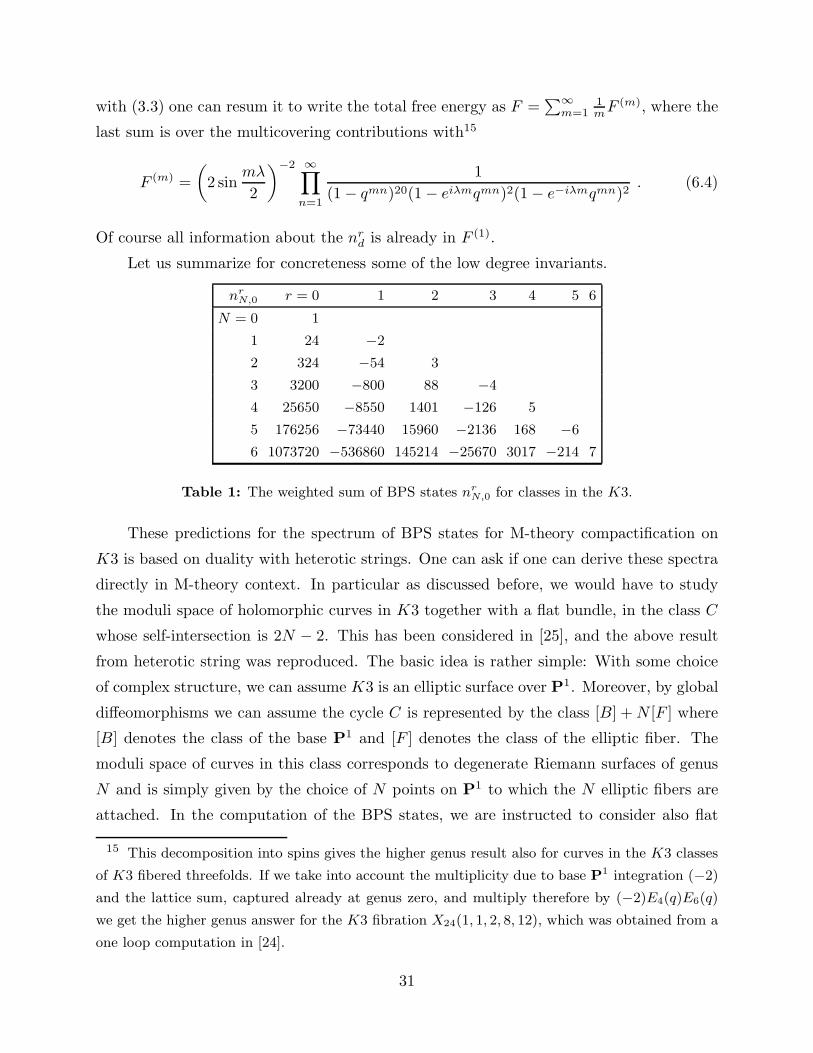
Let us summarize for concreteness some of the low degree invariants.

nrN,0 r = 0 1 2 3 4 5 6

N = 0 1

1 24 −2

2 324 −54 3

3 3200 −800 88 −4

4 25650 −8550 1401 −126 5

5 176256 −73440 15960 −2136 168 −6

6 1073720 −536860 145214 −25670 3017 −214 7

Table 1: The weighted sum of BPS states nrN,0 for classes in the K3.

These predictions for the spectrum of BPS states for M-theory compactification on

K3 is based on duality with heterotic strings. One can ask if one can derive these spectra

directly in M-theory context. In particular as discussed before, we would have to study

the moduli space of holomorphic curves in K3 together with a flat bundle, in the class C

whose self-intersection is 2N − 2. This has been considered in [25], and the above result

from heterotic string was reproduced. The basic idea is rather simple: With some choice

of complex structure, we can assume K3 is an elliptic surface over P1. Moreover, by global

diffeomorphisms we can assume the cycle C is represented by the class [B] +N [F ] where

[B] denotes the class of the base P1 and [F ] denotes the class of the elliptic fiber. The

moduli space of curves in this class corresponds to degenerate Riemann surfaces of genus

N and is simply given by the choice of N points on P1 to which the N elliptic fibers are

attached. In the computation of the BPS states, we are instructed to consider also flat

15 This decomposition into spins gives the higher genus result also for curves in the K3 classes

of K3 fibered threefolds. If we take into account the multiplicity due to base P1 integration (−2)

and the lattice sum, captured already at genus zero, and multiply therefore by (−2)E4(q)E6(q)

we get the higher genus answer for the K3 fibration X24(1, 1, 2, 8, 12), which was obtained from a

one loop computation in [24].

31

bundles on the Riemann surface. In this degenerate limit, that choice is easy: it simply

corresponds to the choice of a flat bundle on each elliptic fiber. That in turn is equivalent

to a choice of a point on a dual elliptic fiber. All said and done, the choice of N points

on P1 and a point on the dual elliptic fiber over each point, shows that the moduli space

of curves with the flat bundle is equivalent to the choice of N points on the T -dual K3.

Since the ordering of the points are immaterial, this corresponds to the N fold symmetric

product of K3, or more precisely, the Hilbert scheme of N points on K316. Thus the

moduli space is given by

M = HilbN (K3)

The cohomology of this space can be identified in the usual way [26] with the Hilbert space

of 24 oscillators at levelN , and exactly reproduces the above results for the heterotic string.

Moreover the SU(2)L×SU(2)R decomposition can also be deduced from the corresponding

decomposition for the cohomology of a single copy ofK3. With the identification of SU(2)L

with the elliptic fiber direction and SU(2)R with the base directions, we immediately get

the decomposition

24 → 20(0, 0) + (1

2,1

2),

as this is the unique representation whose diagonal SU(2) content is (1) ⊕ 21(0), the

Lefschetz representation of K3, while the SU(2)R content of left-spin 1/2 is (1/2), the

Lefschetz representation on the base M = P1. This reproduces the result based on duality

with heterotic strings given above.

In [18], the coefficients cN of I0, which as discussed is the Euler characteristic of

HilbN (K3), were related to genus zero curves coming from degenerate genus N curves

with exactly N nodes. As the N continuous parameters of the moduli space PN of the

genus N curve are completely killed by the imposition of the N nodes, this eventually

leads to the counting of points. Here we consider the intermediate cases, the genus N − δ

curves, where we impose 0 ≤ δ ≤ N nodes. As this leaves a δ dimensional moduli space,

an appropriate virtual fundamental class on this space is needed to reduce the dimension

to 017. The formula (5.2) is equivalent to the assumption that the obstruction bundle in

16 It would be nice to make this argument mathematically more rigorous. What has to be

checked is that this correspondence continues to hold when several fibers are allowed to coincide.

The details will require a mathematical study of sheaves on non-reduced curves.17 A related problem was considered in [27], where the dimensions of the moduli space was

reduced to 0 by forcing the curves to go through k − δ points.

32

the case of a smooth moduli space is the cotangent bundle, since the Euler class of the

cotangent bundle is the Euler characteristic of the moduli space up to sign.

For example, the coefficients in (6.2) correspond to invariants nr3 associated to genus

r = 0, 1, 2, 3 curves obtained by putting nodes on the degree d = 3 genus g = 3 curve.

The moduli space of such curves has dimension r = 0, 1, 2, 3, and the virtual fundamental

class has the same codimension. So the nr3 (and multiple cover/bubbling contributions)

can be thought of as computable by taking the virtual class and performing an additional

localization on the positive dimensional moduli space Mδ of curves with δ nodes. By the

discussion of Section 4 and 5, we can instead calculate these using the invariants e(C(k)[N ])

for k ≤ δ. In other words, in this case we have two geometric models for computing nr[N,0]:

One is based on the Hilbert scheme of N points on K3, which we have already discussed,

and it agrees with the predicted answer from heterotic string. Another way to compute

these numbers is to follow the strategy developed in previous sections and relate these

numbers to e(C(k)[N ]). This will be useful, as it will also tell us how in some cases where

these spaces are singular, we may nevertheless define unambiguous answers.

Let’s check a few cases of these numbers. For any N , we have M = PN .

For N = 0, the moduli space is a point, and n00 = 1.

For N = 1, the moduli space is M = P1, giving n11 = −2 by (5.3). Choosing the

complex structure so that the K3 is elliptically fibered and our family of curves is the fiber

class, we see that C is just the K3. So from [18] or from (5.4), we get n01 = e(C) = 24.

For N = 2, we again get n22 = 3 (and more generally, ngg = (−1)g(g + 1)). Let us

choose the complex structure to be that of S = P(1, 1, 1, 3)[6]. The projection π : S → P2

onto the first 3 coordinates is a 2-1 cover. The inverse images C via π of the lines in

P2 define the genus two curves. To see this, letting H be the hyperplane class of P2 we

compute

C2 = (π∗(H))2 = π∗(point) = 2,

since 2 points of S lie over a point of P2. Since C2 = 2N − 2 = 2, this verifies that the

genus is N = 2. To calculate C, as usual we project C onto S and note that the fiber is

always P1 as follows. Given a point p of a curve C (so that (p, C) ∈ C), the curves C

through p are in 1-1 correspondence with the lines of P1 through π(p), and this is always

a P1. This gives e(C) = e(S)e(P1) = 48, and by (5.4), we get n12 = −(48 + 2 · 3) = −54.

But now something interesting happens. The space C(2) is not a projective bundle

over Hilb2(S). To see this, let’s pick a point Z of Hilb2(S). This usually projects via π to

33

a point Z ′ of Hilb2(P2). When this happens, there is a unique line ℓ connecting the two

points of Z ′ in P2, hence a unique curve C = π−1(ℓ) in S passing through the two points of

Z. So we might have thought that C(2) is isomorphic to Hilb2(S), with Euler characteristic

324. But this is not true! If the point Z consisted of the 2 points of π−1(p) for any point

p ∈ P2, then it maps via π to just the point p of P2. There is a P1 of lines through p,

whose inverse images via π are a P1 of curves in S through Z. In other words, there is an

isomorphic copy of P2 embedded in Hilb2(S) via the map p 7→ π−1(p), and each of these

points gets replaced by a P1 in C(2). It is not difficult to see that C(2) is the blowup of

Hilb2(S) along P2. This tells us that C(2) is smooth, so that (5.4) applies. It also tells us

that e(C(2)) = e(Hilb2(S)) + e(P2) = 324 + 3 = 327. Now, (5.4) gives n02 = 324. We will

give a physical way to calculate e(C(2)) using K3 × T 2 soon.

In general, if the map C(k) → Hilbk(K3) is a projective bundle, then we see that C(k)

is smooth, and its Euler characteristic is (g− k+ 1)e(Hilbk(K3)), where g is the genus N .

We can then calculate ng−kg using (5.5). If it is not a projective bundle, then there are two

problems. First, the Euler characteristic is more difficult to calculate. Second, and more

seriously, the space C(k) need not be smooth, so there may be a virtual fundamental class

to calculate instead of the Euler characteristic and our formulas need not be valid.

Let’s check N = 3. We have M = P3 and n33 = −4. It is not hard to see (and we

will check presently) that C and C(2) are projective bundles, so that e(C) = 3 · 24 = 72

and e(C(2)) = 2 · 324 = 648. This gives, by (5.4), n23 = 72 + 4 · 4 = 88, and n1

3 =

−(648 + 2 · 72 + 2 · 4) = −800.

To compute e(C(3)), we choose our K3 to have the complex structure of a degree 4

hypersurface S ⊂ P3, and the genus 3 curves C to be the plane sections of S (which are all

degree 4 plane curves). Note that there is a P2 of planes passing through any point of S,

and a P1 of planes containing any 2 points of S, verifying the projective bundle structure

on C and C(2) just mentioned. Given three points of S, there is typically a unique plane

containing these points (the plane they span), but this fails when the 3 points lie on a line

ℓ, in which case we get a P1 of planes. In other words, the set of triples of collinear points

in S forms a subset T of Hilb3(S), and we replace T by a P1 bundle over T to get C(3).

Thus e(C(3)) = e(Hilb3(S)) + e(T ).

There is an alternative way to describe T . Let p0 ∈ S be arbitrary. Let ℓ be any line

containing p0 (for fixed p0, there is a P2 of such lines). Then ℓ∩ S consists of 4 points, of

which p0 is one of them. So there are 3 remaining points p1, p2, p3, which collectively give

a point of T . Thus the data of T is a point of S and a point of P2, and so T is smooth

34

and e(T ) = e(S)e(P2) = 72. Furthermore, it is again straightforward to check that C(3) is

the blowup of Hilb3(S) along T , so is smooth. Thus e(C(3)) = 3272 (which we will check

soon by a different method), and by (5.4), n03 = 3272 + 0 − 72 + 0 = 3200.

In principle these calculations can be continued to higher N , at the expense of having

to use increasingly difficult projective geometry to complete the calculation. We will return

to more of these calculations shortly when we see that many of the moduli spaces M for

K3 × T 2 with M 6= 0 are precisely the relative Hilbert schemes C(k) for K3!

6.2. More general H2 classes in K3 × T 2

We will now relax the assumption that M = 0 and also consider the case where the

M2 brane wraps M times around the T 2. When M = 0 we used three ways to compute

it in the previous section: One was the duality with heterotic strings. The other was

the direct definition in M-theory, leading to Hilbert scheme of K3 and the third one,

was based on the methods we developed in this paper. The first two approaches gave a

complete answer, whereas the third approach was somewhat incomplete (even though in

principle one should be able to push that program of computation sketched in some cases

in the previous section). For the case when M 6= 0 it turns out we only know one method

to compute the exact answer and that is based on duality between M-theory on K3 × T 2

and Type IIB string on K3 × S1. The other two methods, are more difficult and we do

not know how to use the direct definition of BPS states of M2 brane to obtain the results

predicted by this duality. We will discuss aspects of these computations in special cases

below. But first we show what the duality between M-theory and type IIB predicts for all

the numbers nr[N,M ] defined before.

M-theory on T 2 is dual to type IIB on S1. Through this duality the M2 brane in 9

dimensions, gets mapped to a D3 brane wrapped around S1. Moreover the momentum

quantum number around S1 of type IIB gets mapped to the quantum number of the M2

brane wrapping number over T 2. Now consider compactifying further on a K3. Then an

M2 brane wrapped in some 2-cycle class of K3×T 2 given by [C,M ], gets mapped via this

duality to D3 branes wrapped around C × S1 carrying momentum M around S1. In fact,

in the type IIB setup, these are exactly the class of black holes that were studied in [28].

Let us consider the limit where the K3 is small. In this limit we have an effective leftover

1 + 1 dimensional worldvolume of the D3 brane which is a supersymmetric sigma model

on SymN (K3). Thus the moduli of D3 branes in the class C of K3 with C2 = 2N − 2

is given by SymN (K3) × R4, where the extra R4 comes from the position of the D3

35

brane in the rest of the space. Thus the low energy dynamics of the 1+1 dimensional

effective theory is a supersymmetric sigma model on this space. We are considering the

spatial direction to be wrapped over an S1 and we are looking for states which preserve

1/4 supersymmetry in the full theory, which correspond to states which preserve 1/2

supersymmetry in the 1+1 dimensional sigma model. These come from states with purely

left-moving oscillator excitations, and restricting to the ground states of the right-moving

Hilbert space. Moreover if we are interested in M2 brane BPS states with wrapping number

M around T 2, we should look at left-moving oscillator excitationM . The SU(2)L×SU(2)R

symmetry is realized in the Hilbert space of the sigma model by a left-moving current

algebra which realizes SU(2)L and a right-moving current algebra realizing SU(2)R [29],

as far as the degrees of freedom is concerned on the symmetric product of K3’s. However

for the R4 factor, the SU(2)L current algebra is a right-moving current and the SU(2)R

current is a left-mover18. Summing over the R states with (−1)FR is exactly the definition

of the elliptic genus of the sigma model on SymN (K3) × R4. It was in fact the elliptic

genus that was used to verify the predictions for black hole entropy [28][29]! So in this case

we see that the left/right asymmetric treatment of the SU(2)L × SU(2)R is exactly the

same as the useful elliptic genus index for supersymmetric sigma models, which has the

required stability under deformations which allows one to predict at least a lower bound

for the black hole entropy. The spinning quantum number of the black hole gets mapped

in this case to the J3L quantum number. We will use this link with black holes in the

next section to connect the growth of nrd with predictions based on black hole entropy for

M-theory compactification on a general Calabi-Yau 3-fold.

Due to interest from black hole physics the elliptic genus of symmetric products of

K3 has been computed, including the modification due to the J3L quantum number [30].

Let us denote the elliptic genus of a general manifold M

χ(M ; q, y) = TrH(M)(−1)F yFLqH =∑

M≥0,l∈Zc(M, l)qMyl (6.5)

18 The reason for this switch, relative to the K3 degrees of freedom is that in the gauge theory

language in 6 dimensions (as in the dual D1–D5 brane dual systems), K3 degrees of freedom

come from the Higgs branch and the R4 from the Coulomb branch, and the fermions in these

two multiplets have opposite 6-dimensional chiralities. This translates to the statement that the

SO(2) and SO(4) chiralities are oppositely correlated in the two cases. This in particular means

that the left-moving fermions do not carry any SU(2)L quantum number for the R4 sigma models.

Of course the bosonic oscillators are vectors and do carry both quantum numbers.

36

then the orbifold construction of [30] gives for the N -fold symmetric product SymN (M)

∞∑

N=0

pNχ(SNK3; q, y) =∏

N>0,M≥0,l∈Z

1

(1 − pNqMyl)c(N·M,l) . (6.6)

The elliptic genus of the K3 can be easily made concrete from an orbifold representa-

tion of the K3 (e.g. K3 = T4/Z2) or a Landau-Ginzburg description as

χ(K3; q, y) = 24

(θ3(q, y)

θ3(q)

)2

− 2θ44(q) − θ4

2(q)

η4

(θ1(q, y)

η

)2

.

We note the first terms of this expansion

q0 :2

y+ 20 + 2 y = 2

[1

2

]+ 20 [0] , q1 :

20

y2− 128

y+ 216 − 128 y + 20 y2 .

Clearly the q0 part of (6.6) gives (6.4) back. So far we ignored the fact that the momentum

can be distributed in the space time directions as well. Taking this into account (and noting

as discussed before that the SU(2)L current algebra is not active as far as the left-moving

fermions from the R4 part are concerned) we get for the single cover contribution

F (1) =

(2 sin

λ

2

)−2 ∏

k>0n>0m≥0,l∈Z

(1 − qk)4

(1 − eiλqk)2(1 − e−iλqk)21

(1 − pnqmeilλ)c(n·m,l)

=:

(2 sin

λ

2

)−2 ∑

N≥0,M≥0,L∈ZcN,M,L p

NqMeiLλ

. (6.7)

As with (6.4), we can sum over all multicoverings F (m) to obtain the free energy. Moreover

we may multiply by a lattice theta functions if we wish to exhibit the sum over classes in

H2(K3, Z) .

Let us recapitulate the dictionary which relates this to the counting of M2 branes of

M-theory in K3 × T 2. N corresponds to the genus g of a smooth curve in the K3, which

after a suitable complex structure deformation can be always thought as a curve C with

degree N with respect to an elliptic K3’s fiber class which has degree 1 in the base class.

The powers M correspond to the degree with respect to the T 2. The powers L (note the

y → 1/y symmetry) correspond to the number of nodes δ, and for a given class [M,N ] we

have δ = N +M − L.

Let us consider the case δ = 0 first. Geometrically the moduli space of these curves

is modeled by C(M)[N ] , the degree M relative Hilbert scheme of the universal curve. To see

37

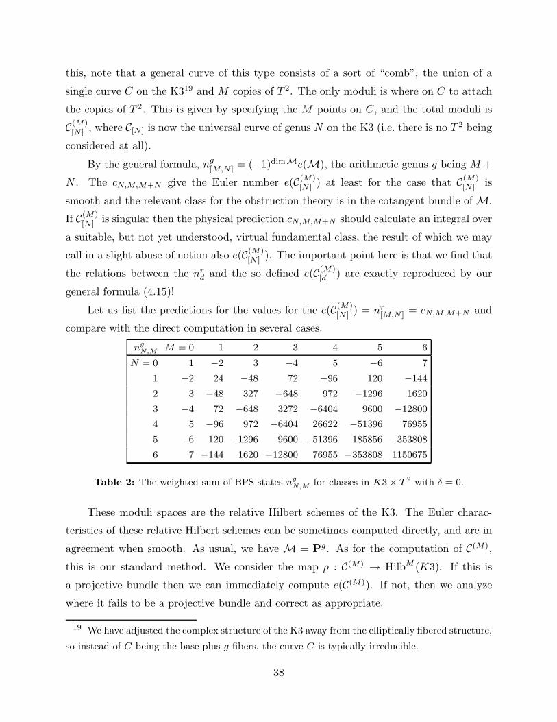
this, note that a general curve of this type consists of a sort of “comb”, the union of a

single curve C on the K319 and M copies of T 2. The only moduli is where on C to attach

the copies of T 2. This is given by specifying the M points on C, and the total moduli is

C(M)[N ] , where C[N ] is now the universal curve of genus N on the K3 (i.e. there is no T 2 being

considered at all).

By the general formula, ng[M,N ] = (−1)dimMe(M), the arithmetic genus g being M +

N . The cN,M,M+N give the Euler number e(C(M)[N ] ) at least for the case that C(M)

[N ] is

smooth and the relevant class for the obstruction theory is in the cotangent bundle of M.

If C(M)[N ] is singular then the physical prediction cN,M,M+N should calculate an integral over

a suitable, but not yet understood, virtual fundamental class, the result of which we may

call in a slight abuse of notion also e(C(M)[N ] ). The important point here is that we find that

the relations between the nrd and the so defined e(C(M)[d] ) are exactly reproduced by our

general formula (4.15)!

Let us list the predictions for the values for the e(C(M)[N ] ) = nr[M,N ] = cN,M,M+N and

compare with the direct computation in several cases.

ng

N,M M = 0 1 2 3 4 5 6

N = 0 1 −2 3 −4 5 −6 7

1 −2 24 −48 72 −96 120 −144

2 3 −48 327 −648 972 −1296 1620

3 −4 72 −648 3272 −6404 9600 −12800

4 5 −96 972 −6404 26622 −51396 76955

5 −6 120 −1296 9600 −51396 185856 −353808

6 7 −144 1620 −12800 76955 −353808 1150675

Table 2: The weighted sum of BPS states ng

N,M for classes in K3 × T 2 with δ = 0.

These moduli spaces are the relative Hilbert schemes of the K3. The Euler charac-

teristics of these relative Hilbert schemes can be sometimes computed directly, and are in

agreement when smooth. As usual, we have M = Pg. As for the computation of C(M),

this is our standard method. We consider the map ρ : C(M) → HilbM (K3). If this is

a projective bundle then we can immediately compute e(C(M)). If not, then we analyze

where it fails to be a projective bundle and correct as appropriate.

19 We have adjusted the complex structure of the K3 away from the elliptically fibered structure,

so instead of C being the base plus g fibers, the curve C is typically irreducible.

38

Letting C be the universal curve on a general K3 of genus N , we have seen from the

comb description that M = C(M), leading to ng[M,N ] = e(C(M)) when C(M) is smooth. In

particular, this occurs if N is large, with the asymptotic formula

ng[M,N ] = (−1)N+M (N + 1 −M)e(HilbM (K3)), N >> 0

which is consistent with the appearance of the columns of the above table. The de-

viations from this formula occur when there is not a projective bundle structure for

C(M) → HilbM (K3). We have already explained this for M = N = 2 and for M = N = 3.

Let’s look at N = 4 and M = 3. We choose the complex structure to be that of

S = P4[2, 3], the intersection of a degree 2 hypersurface Q and a degree 3 hypersurface T .

The curves of genus 4 are the hyperplane sections. By dimension reasons, we might expect

the fibers of C(3) → Hilb3(S) to be P1, but if the 3 points happen to lie on a straight line,

there is a P2 of hyperplanes through the line, giving a fiber of P2 rather than P1. Let’s call

this locus B ⊂ Hilb3(S). Now, if 3 points of S lie on a line ℓ, then the quadratic equation

defining Q has at least 3 zeroes on the line ℓ, hence vanishes identically. Thus ℓ ⊂ Q.

Conversely, any line contained in Q will meet S in 3 points (the three points where the line

meets T ). This shows that B is the set of lines contained in Q. So C(3) is a P1 bundle over

Hilb3(S), except over B where it is a P2 bundle. This gives e(C(3)) = 2·e(Hilb3(S))+e(B).

We can use standard techniques in algebraic geometry [31] and the Schubert software [32]

to compute e(B) = 4. This gives the invariant 6404, in agreement with the table.

We can also check theN = 1 row. We have by (5.3) nM+1[1,M ] = (−1)M+1e(C(M)), where C

is the universal curve of the elliptic fibration. If C is a smooth fiber, then the corresponding

fiber of C(M) is the M th symmetric product of C, which has Euler characteristic 0. So it

is only the 24 singular fibers that contribute to e(C(M)). Each of these singular fibers C

has exactly one node, so e(HilbM (C)) = M by the discussion in the paragraph following

(5.16). This gives e(C(M)) = 24M , or nM+1[1,M ] = (−1)M+124M , in agreement with the table.

Note that the symmetry of the table is immediate from duality and our calculations,

but the geometric content of this symmetry is non-trivial, even in identifying the N = 1

row with the M = 1 column.

We can also consider the more difficult situation where we put nodes δ = N+M−L >0. Some invariants for δ = 1 are given in the table below.

39

ng−1N,M M = 0 1 2 3 4 5 6

N = 0 0 0 −6 16 −30 48 −70

1 24 0 216 −432 768 −1200 1728

2 −54 720 −162 5712 −9768 15552 −22680

3 88 −1488 11832 −4368 83496 −135456 204872

4 −126 2376 −23016 138696 −65112 884184 −1398486

5 168 −3360 36000 −258048 1292712 −701856 7546536

6 −214 4440 −50328 396392 −2324790 10160160 −6086258

Table 3: The weighted sum of BPS states ng−1N,M for classes in K3 × T 2.

Note that the M = 0 column reproduces the K3 results found earlier.

7. Black Hole Entropy and Topological Strings

As discussed in the previous section in the context of M-theory compactification on

K3×T 2, the spectrum of M2 branes wrapped around various cycles for large enough cycle

classes would physically correspond to black holes. Moreover the SU(2)L content of the

BPS state corresponds to the spin of the black hole. In such a case the growth of wrapped

M2 branes in a given H2 class and with given spin is anticipated by the Bekenstein-

Hawking entropy of macroscopic black holes, which has been verified. Moreover, there are

index-like quantities appearing in topological string theories, computed as a sum over the

right-moving states with (−1)FR , which in the type IIB setup is perturbation invariant

and is related to the computation of the elliptic genus. These are exactly the kind of

computations which yield black hole entropy in the regimes where string perturbation

breaks down.

It is thus natural to expect that this relation between BPS states in M-theory com-

pactification on a general Calabi-Yau threefold continue to hold, namely the growth of the

left BPS degeneracy with fixed SU(2)L content but summed over right SU(2)R quantum

numbers with (−1)FR will also yield the black hole entropy. In what we shall write here

we will not worry about numerical constants in the formula for the growth of black hole

entropy.

If we consider the macroscopic prediction for black hole entropy coming from a large

charge d >> 1 and for a given J3L = m spin one obtains [29], in the regime d >> m and

d >> 1,

Nd,m ∼ exp√d3 −m2 (7.1)

40

This is meant to convey the exponential growth and its dependence in uniform rescaling

of d and m, and is valid up to numerical coefficients in the exponent. Also there may be

a sub-leading power law correction prefactor in front of the exponent.

One can try to compare this macroscopic prediction with the microscopic prediction.

Since the SU(2)L content of the black hole entropy is captured by the numbers nrd, we can

compare with the total number of BPS states with charge d and with J3L spin m. All we

need to do is to recall that the full representation of the BPS states with charge d is given

by

R = [

g∑

r=0

nrdIr] ⊗ I1 (7.2)

This sum is finite, as for a given degree there is a maximum genus curve which realizes it.

Moreover if we consider the Ig content of the state we have

TrIkyJ

3L = (y

12 + y

−12 )2k

This in particular means that the number of states in Ik with J3L = m spin is given by

(2k

k +m

)

Applying this to (7.2) we see that the number Nd,m is given by

Nd,m =∑

r

nrd

(2r + 2

r + 1 +m

)

Comparing this with the growth expected from macroscopic considerations (7.1), we get

the prediction in the limit d >> 1, d >> m

∑

r

nrd

(2r + 2

r + 1 +m

)∼ exp

√d3 −m2 (7.3)

This is a very delicate sum, in that nrd are typically very big numbers for d large, which

alternate in sign when one changes g by one unit, as we have seen in many examples in

this paper. It is known that nrd for a fixed r grows with large d as exp(d). This however,

is not in contradiction with the prediction (7.3) as one is summing over all non-vanishing

r, and for large d’s the allowed range in r is also large. In other words one is considering a

different region of parameters and the equation (7.3) is a new prediction of the growth of

these numbers in a different direction. It would be interesting to verify them (some special

cases of this formula for Calabi-Yau threefold has been verified in [33] in the context of

elliptic 3-folds).

41

8. Computations in local Calabi-Yau geometries

In this section we will apply the techniques developed in sections 4 and 5 to local

Calabi-Yau geometries. By a local Calabi-Yau model we mean the total space O(KB) → B

of the canonical line bundle fibered over a (two) dimensional Fano20 variety B. For the base

B we discuss here del Pezzo surfaces P2, P1×P1 and En, the blow up of P2 in n = 1, . . . , 8

points21. To calculate the invariants for a curve with δ nodes we have to calculate e(C(k))

for k ≤ δ, which is easy when there is a bundle structure ρk : C(k) → Hilb(k)(B). For a

given degree d we find in general a bound δ < δmax(d) for which this is true. For instance,

on P2 the first restriction comes from δmax(6) = 8. In general one can show that in this

case δmax(d) = d+2. Another complication arises when the curves are reducible. However

we found a systematic procedure to account for the corrections due to reducible curves,

which gives the expected answer whenever e(C(k)) could be calculated using the bundle

structure. The information from these calculations were sufficient to fix the B-model

ambiguity up to genus g = 4, 5 in the examples. When there is no bundle structure for

C(k) the modeling of these spaces becomes more complicated. While the bundle structure

guarantees smoothness, we find in examples22 that some of the spaces lacking the bundle

structure are singular. Hence the Euler number e(C(k)) has to be replaced by an integral∫[C(k)]vir

ctop over a suitable virtual fundamental class. We have not attempted to define

this virtual fundamental class. However inK3×T 2 case the quantity∫[C(k)]vir

c appeared in

two places in our calculation fitting exactly our approximation ofH∗(J (C)) as expressed in

C(k) by (4.15). We are therefore optimistic that there is natural definition of∫[C(k)]vir ctop

for the non-smooth C(k) in the general case, which calculates the nrd invariants by the

formulas in sections 4,5.

8.1. Basic concepts

First we need to calculate the Euler number of the moduli space e(M) for the

non-degenerate curves C, which are embedded in the surface B. More precisely, these

20 The condition for B to be Fano can be relaxed, see [34].21 Quantum intersection rings on these surfaces were discussed in [35]. In these cases the

dimension of the moduli space of the curves is reduced to zero by requiring the curves to go

through fixed points. There is no obvious relation between these invariants and the ones we

calculate and relate to M-theory BPS states [36].22 C(8) at d = 6 and C(9) at d = 7 on P

2 to be discussed below.

42

curves are characterized by the fact that their geometric genus and their arithmetic

genus coincide. We obtain the dimension of the deformation space PH0(O(C)) from

χ(O(C)) =∑n

i=0(−1)ihi(O(C)) under the assumption that H1(O(C)) = H2(O(C)) = 0.

This is true on del Pezzo surfaces with general moduli [37]. Then, using adjunction

C2 +KC = (2g − 2)

and the Riemann-Roch formula

χ(O(C)) =C2 −KC

2+ 1,

we obtain χ(O(C)) = g + d, where d is the degree of the curve with respect to the anti-

canonical class −K of B. Since the moduli space is obtained by projectivizing H0(O(C)),

we get as the result

e(M) = e(Pg+d−1) = (g + d). (8.1)

To be concrete, recall that the classes on a En del Pezzo are the P2 hyperplane class

H and the exceptional divisors of the blowups ei in n points p1, . . . , pn, with H2 = 1 and

eiej = −δij (for P1 × P1 see the later discussion). A curve of multidegree (a; b1, . . . , bn)

refers to the class of curves obtained from blowing up the plane curves of degree a which

pass through the point pi with multiplicity bi. These curves have class aH −∑ biEi. We

will typically rearrange the order of points to write the bi in nonincreasing order. We

will also omit the bi which are 0. And we will use exponential notation bk to refer to a

subsequence of k copies of b. The exceptional divisors ei do not fit into this classification

scheme and will be denoted separately. To follow the subsequent discussion one needs

an overview over the low degree classes in the del Pezzos surfaces, which we provide in

Appendix A. They are ordered with respect to their arithmetic genus

g =(a− 1)(a− 2)

2−

n∑

i=1

bi(bi − 1)

2(8.2)

and their degree with respect to the anticanonical class of the del Pezzos −KEn= 3H −

∑ni=1 ei

d = 3a−n∑

i=1

bi . (8.3)

43

Let us consider as an easy example the E1 del Pezzo surface. As it was observed by

mirror symmetry in [38] there are invariants23 n01,a = 2a+1 from curves wrapping 1 times

the base H and a times the fibre H − e1 of the Hirzebruch surface F1 = E1, i.e. since

a = HC and 1 = (H − e1)C these genus zero curves are in the class (a; a − 1) and by

(8.3)(8.1)(5.3) we immediately obtain the mirror symmetry prediction.

To calculate the invariants for curves with one node δ = 1 we need next to determine

the Euler number of the universal curve e(C). We first fix a class [C] with a curve C of

arithmetic genus g and degree d in it. Then we calculate the contribution of a nodal curve

in [C] to the invariant ng−1d at genus g−1 by (4.15) or (5.4)(5.3). In the simplest situation

the nodal curve is irreducible. The space C, comes with a fibration structure as follows.

Fixing the location of a point on the curve gives a linear constraint in the moduli space

Pg+d−1 of the genus g curve. As the point is free to vary over B, C comes with a natural

fibration C → B which, if it is smooth, gives rise to the Euler number

e(C) = e(Pg+d−2)e(B) = (g + d− 1)e(B) . (8.4)

In general if there is the bundle structure ρk : C(k) → Hilb(k)(B) then

e(C(k)) = e(Pg+d−1−k)e(Hilb(k)(B)) (8.5)

with∑k e(Hilb(k)(B))qk =

∏n

1(1−qn)e(B) . The easiest example for the treatment of re-

ducible curves is the calculation of n04 in P2 in section 5.2 (after eq. 5.7). In the case

of general del Pezzo surfaces we have to sum over various classes as will be explained in

Section 8.5 for the case of the E5 del Pezzo when we calculate n04.

8.2. O(−1) ⊕O(−1) → P1

The conifold geometry does not support higher genus curves and the only rational

curve that exists is the P1. Therefore the Fg of the type IIA topological theory24 are

completely governed by the multicover and bubbling contribution of this one rational

curve. In this sense this simplest Calabi-Yau background to which 2-d gravity can be

coupled is completely solved by (2.3) in full accordance to (3.3). It is interesting that

in this case the part of the Fg which follows from the anomaly can be made vanishing

in the holomorphic limit by noting that there is a gauge choice in which all propagators

of Kodaira-Spencer become identically zero, compare [7]. In this sense all holomorphic

information here actually comes from the ambiguity.

23 Which resum to the logarithm capturing the running of the gauge coupling in the N=2 gauge

theory at the appropriate locus in the moduli space.24 Not to be confused with the IIB asymptotic behavior at the locus where an S3 shrinks, which

we discuss in Sections 2,5,6.

44

8.3. Local P2: O(−3) → P2

This is the next simplest case. This geometry supports an infinite number of curves

of different arithmetic genera, making the geometry much more interesting than in the

conifold case.

We first present the result for the invariants. The numbers in the Table 4 marked with

a diamond were obtained with the technique discussed in sections 4 and 5, as explained

in detail below. Once we can fix the holomorphic ambiguity completely for a genus r,

which was possible up to r = 5 in this case (see sect 8.6), the B-model gives an immediate

answer for Fr at all degree d. Using this B-model result integrality of the nrd was checked

up to d = 300. For r = 6, 7, 8 we could determine the ambiguity only up to S = 2, 4, 6

constants, which can be parameterized by the nrd, d = 8, . . .8+Si. Assuming that they are

integer we checked that the B-model gives rise to integer nrd up to d = 300. As a further

check we compared with the calculation in [7], which uses the c = 1 KDV hierarchy and

direct localization techniques. Numbers marked with a star were calculated this way.

The r = 1 numbers listed in Table 4 follow the geometric subtraction scheme (2.4).

The differences in genus 1 between the geometric and the physical subtraction schemes

∆d = (n1d − n∗1

d ) are ∆6 = −10, ∆8 = 231, ∆9 = −10 and ∆10 = 4452 up to given order.

d r = 0 1 2 3 4 5

1 3⋄∗ 0 0 0 0 0

2 −6⋄∗ 0 0 0 0 0

3 27⋄∗ −10⋄

∗ 0 0 0 0

4 −192⋄∗ 231∗ −102⋄

∗ 15⋄∗ 0 0

5 1695⋄∗ −4452⋄

∗ 5430⋄∗ −3672⋄

∗ 1386⋄∗ −270⋄

∗

6 −17064∗ 80948∗ −194022∗ 290853⋄∗ −290400⋄

∗ 196857⋄

7 188454 −1438086 5784837 −15363990 29056614 −40492272

8 −2228160 25301295 −155322234 649358826 −2003386626 4741754985

9 27748899 −443384578 3894455457 −23769907110 109496290149 −396521732268

10 −360012150 7760515332−93050366010 786400843911−5094944994204 26383404443193

45

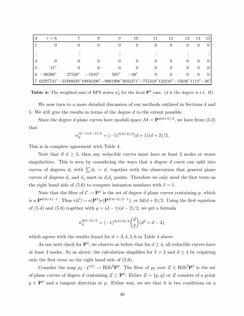
d r = 6 7 8 9 10 11 12 13 14 15

1 0 0 0 0 0 0 0 0 0 0

......

......

......

4 0 0 0 0 0 0 0 0 0 0

5 21⋄ 0 0 0 0 0 0 0 0 0

6 −90390⋄ 27538⋄ −5310⋄ 585⋄ −28⋄ 0 0 0 0 0

7 42297741⋄−33388020⋄19956296⋄−9001908⋄3035271⋄−751218⋄132210⋄−15636⋄1113⋄−36⋄

Table 4: The weighted sum of BPS states nrd for the local P

2 case. (d is the degree w.r.t. H)

We now turn to a more detailed discussion of our methods outlined in Sections 4 and

5. We will give the results in terms of the degree d to the extent possible.

Since the degree d plane curves have moduli space M = Pd(d+3)/2, we have from (5.3)

that

n(d−1)(d−2)/2d = (−1)d(d+3)/2(d+ 1)(d+ 2)/2.

This is in complete agreement with Table 4.

Note that if d ≥ 3, then any reducible curves must have at least 2 nodes or worse

singularities. This is seen by considering the ways that a degree d curve can split into

curves of degrees di with∑di = d, together with the observation that general plane

curves of degrees di and dj meet in didj points. Therefore we only need the first term on

the right hand side of (5.6) to compute instanton numbers with δ = 1.

Note that the fiber of C → P2 is the set of degree d plane curves containing p, which

is a Pd(d+3)−1. Thus e(C) = e(P2)e(Pd(d+3)/2−1), or 3d(d+ 3)/2. Using the first equation

of (5.4) and (5.6) together with g = (d− 1)(d− 2)/2, we get a formula

nd(d−3)/2d = (−1)d(d+3)/2

(d

2

)(d2 + d− 3),

which agrees with the results found for d = 3, 4, 5, 6 in Table 4 above.

As our next check for P2, we observe as before that for d ≥ 4, all reducible curves have

at least 3 nodes. So as above, the calculation simplifies for δ = 2 and d ≥ 4 by requiring

only the first term on the right hand side of (5.6).

Consider the map ρ2 : C(2) → Hilb2P2. The fiber of ρ2 over Z ∈ Hilb2P2 is the set

of plane curves of degree d containing Z ⊂ P2. Either Z = p, q or Z consists of a point

p ∈ P2 and a tangent direction at p. Either way, we see that it is two conditions on a

46

plane curve to contain Z (to say that C contains Z = (p, v) with v ∈ TpP2 means that

p ∈ C and v is tangent to C at p). Thus the fiber is a Pd(d+3)/2−2. This gives

e(C(2)) = e(Pd(d+3)/2−2)e(Hilb2P2)

= 9

(d(d+ 3)

2− 1

).

We get from the second equation of (5.4) and (5.6)

n(d2−3d−2)/2d = (−1)d(d+3)/2

(9

(d(d+ 3)

2− 1

)+ (d2 − 3d− 2) · 3d(d+ 3)

2

+

(d2 − 3d

2

)(d2 − 3d− 3)

(d+ 2

2

)).

In particular, we verify that n14 = 231, as noted earlier, as well as n4

5 = 1386.

Continuing, we have that for d ≥ 5, all reducible curves have at least 4 nodes, so the

calculation for δ = 3 simplifies. We consider the map C(3) → Hilb3P2, and check that

the fiber is always a Pd(d+3)/2−3, yielding e(C(3)) = 22((d+ 4)(d− 1)/2). Using the third

equation from (5.4) and (5.6), we get

nd2−3d−4

2

d = (−1)(d+1)(d+2)

2

(22

(d+ 4)(d− 1)

2+ ((d− 1)(d− 2) − 6) 9

(d(d+ 3)

2− 1

)+

((d− 1)(d− 2) − 4) ((d− 1)(d− 2) − 7)

2

(3d(d+ 3)

2

)+

((d− 1)(d− 2) − 2) ((d− 1)(d− 2) − 6) ((d− 1)(d− 2) − 7)

6

(d+ 2

2

))

(8.6)

In particular, substituting d = 5, 6 into (8.6), we get n35 = −3672 and n7

6 = 27538, see

Table 4.

We recall from Section 5 that we can also handle the situation where there are reducible

3 nodal curves, namely d = 4. The problem is that we have the locus of quartic curves

which are unions of a cubic and a line. We saw how this leads to n4 = −192.

The case of n5 is even more interesting, in that there are two extra components

contained in M6. The first component is the union of degree 2 and degree 3 curves,

contributing n02n

13 = 60, and the second component is the union of lines and degree 4

curves with 2 nodes, contributing n01n

14 = 693. According to (5.6), we substitute d = 5

in (5.5) with δ = 6 and g = 6 and subtract the contributions of 60 and 693, obtaining

n05 = 1695, as in Table 4. The e(C(k)) can be computed as above because in these cases

47

the projection C(k) → HilbkP2 is a bundle of projective spaces and e(HilbkP2) can be

computed by (5.7).

Using (5.5) and (5.6), we can verify nr6 for r ≥ 3. The projection C(k) → HilbkP2 is

again a bundle of projective spaces for k ≤ 7. Recall that this bundle structure implies

that C(k) is smooth, so that our method applies. Thus we have a check of our method for

each δ ≤ 7.

This bundle structure does not occur in general. In the computation of n26, we

encounter the map C(8) → Hilb8P2. Over a general point of Hilb8P2, the fiber is a

P27−8 = P19, as a multiplicity 8 scheme usually imposes 8 conditions on curves of a given

degree. But now suppose the 8 points all lie on a line L, and we identify the projective

space of degree 6 curves containing these 8 points (some of which may coincide). For such

a degree 6 curve, the restriction of its degree 6 equation to L has 8 zeros, hence vanishes

identically. Thus the degree 6 equation contains the equation of the line as a factor, and

we can multiply it by an arbitrary degree 5 polynomial and obtain a degree 6 polynomial

containing the desired 6 points. Since the degree 5 polynomials form a P20, we get a fiber

of P20 rather than P19 in this case.

The lack of a bundle structure for ρ8 : C(8) → Hilb8P2 causes us to ask if our methods

apply in this case. We have to see whether or not C(8) is smooth. Consider the projection

π8 : C(8) → P27 onto the other factor. That is, given an element (C,Z) of C(8), so that

C is a plane curve of degree 6, and Z is a multiplicity 8 scheme in C, i.e. an element of

Hilb8C, put π8(C,Z) = C, where C is now identified with the corresponding element of

M = P27. Since the fibers of π8 are all 8 dimensional, we can see that C(8) has dimension

27 +8 = 35. To show that C(8) is singular, we need only exhibit a single element of C(8) at

which the tangent space of C(8) has dimension strictly greater than 35. Since the tangent

space of C(8) at (C,Z) is naturally identified with the space of first order deformations of

the pair (C,Z), we need only find a (C,Z) for which we can exhibit 36 independent first

order deformations.

Towards this end, for C we take a degree 6 curve l(x1, x2, x3)2f(x1, x2, x3) = 0, where

l is linear and f is homogeneous of degree 4 in the homogeneous coordinates (x1, x2, x3)

of P2. For Z we take any 8 points on the line l(x1, x2, x3) = 0, which can possibly occur

with multiplicity.

Note first that we have 16 independent deformations obtained by moving these 8

points arbitrarily in P2 while keeping C fixed. This is because of the factor of l2, which

ensures that all motions of the points stay within C to leading order. Then we take the 20

48

deformations noted above, where we fix Z, but now vary the degree 6 curve to an arbitrary

curve of the form l(x, y, z)g(x, y, z) = 0, where g is homogeneous of degree 5. These 20

deformations are in fact honest deformations, not just first order deformations. Combining

these two classes of first order deformations where we deform C and Z separately, we have

all together the needed 16 + 20 = 36 deformations.

While our methods gave the correct results for singular moduli spaces arising from

isolated nodal curves in Section 4, we are not so lucky this time. The calculation based on

(5.5) and (5.6) differs from the value of n26 in Table 4 by 45. We expect that the singular

locus of C(8) provides a correction term to (5.6), much as the second term of (5.6) can be

viewed as providing a correction to (5.5). This is a topic for future investigation. If such

a correction can be understood, then we can find Fg for all g geometrically!

We close our discussion of the local P2 with a tantalizing observation about the

correction. We see that the image of the singular locus of C(8) via the projection π8 :

C(8) → P27 is the set of curves which factor into a degree 1 factor with multiplicity 2 and

degree 4 factor. This locus is parameterized by P2 × P14, which has Euler characteristic

45, exactly equal to the desired correction!

But we can’t get too excited yet about this observation. The singular locus itself is a

P8 bundle over this space, since we must consider Z itself, and Hilb8 of a line is just P8.

So the singular locus of C(8) is parameterized by a space of Euler characteristic 9 · 45.

Nevertheless, we suspect that this is more than a coincidence. For d = 7, we see that

C(9) can be singular when the degree 7 curve factors into the square of a linear factor times

a degree 5 factor. This space is parameterized by P2 ×P20, which has Euler characteristic

63. Once again, this is exactly the discrepancy between the value of n67 computed using

the B-model, and the value computed by (5.6)! These examples provide a big hint which

needs to be better understood.

8.4. Local P1 ×P1: O(K) → P1 × P1

As expected from the Segre embedding of P 1 × P 1 into P 3 as a degree 2 surface, we

have the diagonal perturbation of the local P 1×P 1 case, i.e.∑i+j=r n

P 1×P 1

i,j = nX2(1,1,1,1)r ,

which we have checked for genus 0, 1. Still saying it differently it sums up the instantons in

the compact elliptically fibered CY over F0 which survive the limit where the fibre volume

becomes infinite.

49

d r = 0 1 2 3 4

1 −4⋄ 0 0 0 0

2 −4⋄ 0 0 0 0

3 −12⋄ 0 0 0 0

4 −48⋄ 9 0 0 0

5 −240⋄ 136⋄ −24⋄ 0 0

6 −1356 1616 −812 186⋄ −16⋄

7 −8428 17560 −17340 9712 −3156⋄

8 −56000 183452 −302160 307996 −206776

9 −392040 1878664 −4688912 7590720 −8583824

10 −2859120 19027840 −67508988 159995520 −274149876

Table 5: The weighted sum of BPS states nrd for the local P

1 × P1 case.

We now compute the ⋄ numbers in Table 5 geometrically. We recall that a curve of

bi-degree (a, b) on P1 × P1 has total degree d = a + b, genus g = (a − 1)(b − 1), and

M = P(a+1)(b+1)−1. By (5.3), this gives a contribution of (−1)(a+1)(b+1)−1(a+ 1)(b+ 1))

to n(a−1)(b−1)a+b .

If d = 2k is fixed, then relative to all possibilities for d = a+b, the choice (a, b) = (k, k)

gives the maximum possible genus (k − 1)2. Thus

n(k−1)2

2k = (−1)k2+2k(k + 1)2 = (−1)k(k + 1)2.

This verifies our results for k = 1, 2, and 3.

If d = 2k + 1, then the maximal genus k(k − 1) is attained for (a, b) = (k + 1, k) or

(k, k + 1). We may as well consider one of these cases and multiply the result by 2. By

(5.3) we get

nk(k−1)2k+1 = −2(k + 1)(k + 2),

where the definite sign follows since (k+ 2)(k+ 1) is always even. This verifies our results

for k = 0, 1, 2.

We next turn to curves with 1 node, δ = 1. If d = 2k+1, then the only contributions to

nk(k−1)−12k+1 come from (a, b) = (k+1, k) or (k, k+1). If d ≥ 5, there are no reducible curves

of these bi-degrees with only 1 node. We restrict to the first case and will later multiply the

contribution by 2. The map C → P1 ×P1 has fiber over p the space of curves of bi-degree

(k + 1, k) which contain p, a P(k+2)(k+1)−2. This leads to e(C) = 4((k + 2)(k + 1) − 1) =

4(k2 + 3k + 1). We get

nk2−k−1

2k+1 = 2(4(k2 + 3k + 1) + (2k(k − 1) − 2)(k + 2)(k + 1)

),

50

which in particular verifies n15=136.

If d = 2k and k ≥ 2, a new interesting possibility arises, which is typical in the sequel.

We get contributions to n(k−1)2−12k some of which have δ = 0, while others have δ = 1. The

former type comes from (a, b) = (k+1, k−1) or (k−1, k+1). This gives a contribution of

2(−1)k(k+2)−1k(k+2) by (5.3). The δ = 1 contribution comes from (a, b) = (k, k), and we

get (−1)(k+1)2−2(4((k+ 1)2 − 1) + (2(k− 1)2 − 2)(k+ 1)2) from the first equation in (5.4)

together with (5.6), as there are no reducible curves of this bi-degree with only 1 node.

Combining these two contributions gives

nk2−2k

2k = (−1)k(k+2)−1(2k(k + 2) + 4

((k + 1)2 − 1

)+(2(k − 1)2 − 2

)(k + 1)2

),

which agrees with Table 5 for k = 2, 3.

We next consider the case of d = 7, g = 4. Here there are the possible bi-degrees

(4, 3) and (5, 2). Since the latter case already has g = 4, we get a moduli space M = P17,

which gives a contribution of −18 by (5.3). Curves of bi-degree (4, 3) have genus g = 6 and

M = P19, with e(M) = 20. We get as usual e(C) = 19 · 4 = 76 and e(C(2)) = 18 · 14 = 252

(we have used e(Hilb2(P1 × P1) = 14 here). So the second equation of (5.4) together

with (5.6) gives a contribution of (−1)17(252 + 8 · 76 + 5 · 7 · 20) = −1560, as there are no

reducible curves of this bi-degree with 2 nodes. Combining with the −18 and multiplying

by 2 to account for bi-degrees (3, 4) and (2, 5), we get the consistent answer −3156.

More interesting is the geometric calculation of n05. We have to consider bidegrees (4, 1)

and (3, 2). The first case is handled by (5.3), and we get −10. In the second case, we have

g = δ = 2, e(M) = 12, e(C) = 4 · 11 = 44, e(C(2)) = 14 · 10 = 140. There are also reducible

curves of type (1, 0) ∪ (2, 2) with 2 nodes. By (5.3), we have n01,0 = −2 and n1

2,2 = 9. So

by the second equation in (5.4) and (5.6), we get n03,2 = −(140 − 12) − (−2) · 9 = −110.

Thus n05 = 2(n0

3,0 + n04,1) = −240, in agreement with Table 5.

8.5. Other local Del Pezzo geometries: E5, E6, E7, and E8

The E5 del Pezzo:

51

d r = 0 1 2 3 4

1 16⋄ 0 0 0 0

2 −20⋄ 0 0 0 0

3 48⋄ 0 0 0 0

4 −192⋄ 5⋄ 0 0 0

5 960⋄ −96⋄ 0 0 0

6 −5436 1280⋄ −80⋄ 0 0

7 33712 −14816 2512⋄ −160⋄ 0

8 −224000 160784 −51928 8710⋄ −680⋄

9 1568160 −1688800 886400 −274240 51040

10 −11436720 17416488 −13552940 6643472 −2167656

Table 6: The weighted sum of BPS states nrd for the local E5 del Pezzo.

As in P1 × P1, to verify our calculations we need to break up our degrees into sub-

classes. Verification of the En geometries is complicated mainly by the fact that there are

many possibilities contributing to a given degree, and we must consider all the possibilities

for any fixed d that we want to understand.

As typical examples, let us verify n14 and n0

4. We look at the d = 4, g = 1 data first.

We have the class (3; 15) with M = P4 (by Riemann-Roch, one expects M = Pd+g−1 in

general). This verifies n14 = 5 by (5.3). But there is also a δ = 1 contribution to n0

4. We

have C → M with fiber P3, hence

e(C) = e(P3)e(E5) = 4 · 8 = 32.

This gives a contribution of −32 to n04 by the first equation of (5.4) and (5.6).

We next look at the d = 4, g = 0 data. Each of these classes has M = P3. Each P3

gives a contribution of −4. So we have to count numbers of such families. For (2; 12) we

have to choose 2 out of the 5 points at which to put the two ones; there are(52

)= 10 ways

of doing this. For (3; 2, 13) we choose 1 point for the two, and 3 of the remaining points

for the ones, and there are 5(42

)= 20 ways of doing this. Finally, for (4; 23, 12) there are 10

choices. All together, there are 10 + 20 + 10 = 40 distinct d = 4, g = 0 families. The total

contribution is 40(−4) = −160. Combining with the −32, we have −160 − 32 = −192,

which agrees with the calculated value of n04.

52

Now let’s calculate n05. We have for d = 5, g = 1 the families (3; 14), (4; 22, 13), (5, 25)

and we want δ = 1. Including permutations, there are 16 such families. In each case, we

have reducible curves with 1 node:

(3, 14) = (3, 15) ∪E5

(4, 22, 13) = (3, 15) ∪ (1, 12)

(5, 25) = (3, 15) ∪ (2, 15)

Since the curves of type (3, 14) form a P4, and the respective curves E5, (1, 12), and (2, 15)

are all isolated, it follows that the term to be subtracted on the right hand side of (5.6) is

−5. Since e(C) = 5·8 = 40 in each case, we get for each the contribution −40−(−5) = −35

by the first equation of (5.4) and (5.6). Combining this calculation with the more standard

calculations for δ = 0 based on (5.3), we get n5 = 80(5)+16(35) = 960, in agreement with

Table 6.

We can similarly verify all the other cases indicated with a diamond using just these

techniques. We can also check some cases requiring curves with δ > 1 nodes, but these

become increasingly tedious.

The E6 del Pezzo:

d r = 0 1 2 3 4

1 27⋄ 0 0 0 0

2 −54⋄ 0 0 0 0

3 243⋄ −4⋄ 0 0 0

4 −1728⋄ 135⋄ 0 0 0

5 15255 −3132⋄ 189⋄ 0 0

6 −153576 62976 −10782⋄ 789⋄ −10⋄

7 1696086 −1187892 397899 −75114 7641

8 −20053440 21731112 −12055770 4188726 −948186

9 249740091 −391298442 326385279 −179998572 69918830

10 −3240109350 6985791864 −8218296072 6602867631 −3896482536

Table 7: The weighted sum of BPS states nrd for the local E6 del Pezzo.

Note that the second equation in (5.4) is needed for n26, and we get from several

different families of curves, (5.3), the first two equations in (5.4), and (5.6), the result

n26 = 270(−8) + 108(−72) − 846 = −10782, again in agreement with Table 7.

The E7 del Pezzo:

53

d r = 0 1 2 3

1 56⋄ 0 0

2 −272⋄ 3 0

3 3240⋄ −224⋄ 0

4 −58432 12042 −844⋄ 7⋄

5 1303840 −574896 116880 −12112⋄

6 −33255216 26127574 −10554800 2654912

7 930431208 −1163157616 787322120 −358173504

8 −27855628544 51336812456 −52707074296 37805931096

9 878169863088 −2258519658288 3292406219040 −3430645737616

10 −28835628521920 99301270680473 −196037258631040 280764828128124

Table 8: The weighted sum of BPS states nrd for the local E7 del Pezzo.

Again the numbers marked with ⋄ have been checked. Here we determine the number

n35. First let us calculate the contribution of the smooth genus 3 curves with d = 5. From

Appendix A with simple combinatorics follows that there are 1 + 35 + 105 + 7 + 140 + 7 +

140+105+35+1 = 576 curves all with moduli space P7 by (8.1)(5.3), hence contributing

(−1)78·576 = −4608 to n35. Also from the table we read off that there are 7+21+21+7 = 56

genus25 4 curves with d = 5. In fact we have n45 = 56(−1)8 ·9 = 504 from (8.1)(5.3) as there

are no g = 5 curves in classes with d = 5, which could degenerate to g = 4. The universal

curve for each of the of the 56 δ = 1 curves has by (8.4) e(C) = −8 · 10. Application of

(4.15) gives hence a contribution of −56 · 80 − (2 · 4 − 2)504 of the nodal curves to give a

total of n35 = −4608 − 7504 = −12112.

For the E8 del Pezzo surface we obtained

d r = 0 1 2 3 4 5 6 7

1 252⋄ −2⋄

2 −9252⋄ 762⋄ −4⋄

3 848628 −246788 30464 −1548⋄ 7⋄

4 −114265008 76413073 −26631112 5889840 −835236 69587 −2642⋄ 11⋄

Table 9: The weighted sum of BPS states nrd for the local E8 del Pezzo.

25 Note the classical fact that for fixed d these curves are in the representation of the Weyl-group

of E7.

54

The case of the E8 del Pezzo is interesting because it can be easily can be related to

the 12K3, which gives an additional check. Extending [39] it was observed [23] that there

is a modular anomaly in this case for higher genus.

More precisely let F = K 12K3

the fibre (also the canonical class) and B = e9 the base

class of the elliptic half K3 surface. Following [23] we can solve the modular anomaly for

this two parameter subspace and write the contribution to Fr for a fixed base class n as a

quasimodular form P2g+2n−2(E2, E4, E6)q

m2

η12n . In particular we can compare the diagonal

class KE8= F + e9 and test the modular anomaly against the holomorphic anomaly

calculation. We observed complete accordance up to genus 8 degree 10.

8.6. The topological string perspective

In the local case one has for all genera an explicit virtual fundamental class on the

moduli spaces of maps and therefore a direct A-model localization calculation of the topo-

logical string amplitudes at higher genera is in principle possible [7]. At genus zero there is

a virtual fundamental class also for the global case the and equivalence of the A-model and

the B-model calculation was proven [40]. This sort of proof was adapted to the local case

[34]. Hence as an immediate check we can perform in certain cases A-model computations

to compare with. However using the c = 1 KDV hierarchy and localization on the toric

ambient space becomes extremely difficult for high g, where the M -theory calculation is

still very easy, provided that δ < δmax(d).

Furthermore we can consider the B-model and use the M -theory calculation to resolve

the holomorphic ambiguity. The B-model, which has some additional simplifications in

the local case [7], has the virtue that it comes naturally with the analytic techniques on the

complex moduli space of the mirror manifold, which allows us to relate the answers that

we get in the infinite volume limit to physical systems at other degenerations by analytic

continuation. This yields further consistency checks.

To describe the analytic structure we note that the vectors ~a = (a1, a2)

P2 : ~a =

(1

2,2

3

), P1 ×P1 : ~a =

(1

2,1

2

), E5 : ~a =

(1

2,1

2

),

E6 : ~a =

(1

3,2

3

), E7 : ~a =

(1

4,3

4

), E8 : ~a =

(1

6,5

6

),

determine the Picard-Fuchs differential equation, which governs the complex geometry of

the mirror for the local cases(θ3 − z

3∏

i=1

(θ − ai + 1)

)∫

γi

Ω = 0 . (8.7)

55

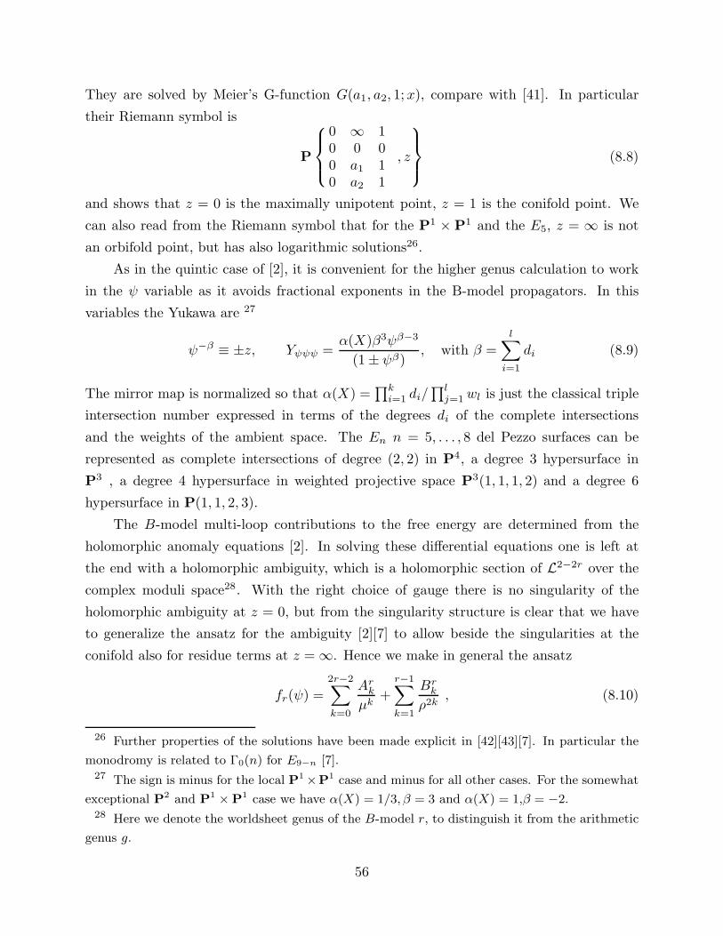
They are solved by Meier’s G-function G(a1, a2, 1; x), compare with [41]. In particular

their Riemann symbol is

P

0 ∞ 10 0 00 a1 10 a2 1

, z

(8.8)

and shows that z = 0 is the maximally unipotent point, z = 1 is the conifold point. We

can also read from the Riemann symbol that for the P1 × P1 and the E5, z = ∞ is not

an orbifold point, but has also logarithmic solutions26.

As in the quintic case of [2], it is convenient for the higher genus calculation to work

in the ψ variable as it avoids fractional exponents in the B-model propagators. In this

variables the Yukawa are 27

ψ−β ≡ ±z, Yψψψ =α(X)β3ψβ−3

(1 ± ψβ), with β =

l∑

i=1

di (8.9)

The mirror map is normalized so that α(X) =∏ki=1 di/

∏lj=1wl is just the classical triple

intersection number expressed in terms of the degrees di of the complete intersections

and the weights of the ambient space. The En n = 5, . . . , 8 del Pezzo surfaces can be

represented as complete intersections of degree (2, 2) in P4, a degree 3 hypersurface in

P3 , a degree 4 hypersurface in weighted projective space P3(1, 1, 1, 2) and a degree 6

hypersurface in P(1, 1, 2, 3).

The B-model multi-loop contributions to the free energy are determined from the

holomorphic anomaly equations [2]. In solving these differential equations one is left at

the end with a holomorphic ambiguity, which is a holomorphic section of L2−2r over the

complex moduli space28. With the right choice of gauge there is no singularity of the

holomorphic ambiguity at z = 0, but from the singularity structure is clear that we have

to generalize the ansatz for the ambiguity [2][7] to allow beside the singularities at the

conifold also for residue terms at z = ∞. Hence we make in general the ansatz

fr(ψ) =2r−2∑

k=0

Arkµk

+r−1∑

k=1

Brkρ2k

, (8.10)

26 Further properties of the solutions have been made explicit in [42][43][7]. In particular the

monodromy is related to Γ0(n) for E9−n [7].27 The sign is minus for the local P

1 ×P1 case and minus for all other cases. For the somewhat

exceptional P2 and P

1 × P1 case we have α(X) = 1/3, β = 3 and α(X) = 1,β = −2.

28 Here we denote the worldsheet genus of the B-model r, to distinguish it from the arithmetic

genus g.

56

where µ = c1(1 ± ψβ) and ρ = c2ψβ.

The finite number of constants Ark, Brk can be fixed by the direct calculation of the nrd,

but at least part of it is also encoded in the universal behavior of Fr at singular loci in the

moduli space. In particular near a conifold singularity one expects [44] from the duality

with the c = 1 critical string theory at the selfdual radius an expansion

FS3(µ) =1

2µ2 log(µ) − 1

12log(µ) +

∞∑

r=2

B2r

(2r − 2)(2r)µ2−2r (8.11)

where B2r/(2r − 2)2r = − 1240

, 11008

,− 11440

, . . . for genus r = 2, 3, 4, . . .. Relative to the

genus expansion of the type II free energy F (t) =∑∞r=0 λ

2r−2Fr(t) (8.11) is a double

scaling limit in which the distance t to the conifold in the moduli space and the string

coupling go to zero while their ratio µ is kept fixed. This selects the corresponding leading

term µ2r−2 form Fr in (8.11). For the local propagators we use the same gauge as in [7]. In

this gauge the singular behavior at the conifold is captured entirely by the ambiguity. The

relation between t = (1±ψβ) and µ can be fixed from the genus zero result by comparing

the asymptotic of the Yukawa coupling with (8.11). We found the simple systematics

µ = (1±ψβ)√α(X)

for the local and µ = i(1±ψβ)√α(X)

for the global cases.

It has been speculated that the next to leading order might be related to correlations

functions of the c = 1 string at the selfdual radius involving discrete states whose SU(2)L×SU(2)R charges could be read off from next to leading order monomial in the perturbations

of the local equations [45]. It would be very interesting to make this more concrete. At

any rate we will report this behavior at the conifold and other singularities along with our

previous results at the large complex structure limit. Beside the verification of the claim

in [44] we find also some regularities for the next to leading order residue. For instance,

we observed up to r = 4 that the Ar2r−3 of the quintic Calabi-Yau threefold are exactly

(4/5) times smaller as the Ar2r−3 for the local P1 ×P1 case, which in turn are identical to

the analogous quantities on the E6 del Pezzo.

For the P2 case we fixed the constants in the ambiguity (3.4) as follows

r Ar0 Ar

1 Ar2 Ar

3 Ar4 Ar

5 Ar6 Ar

7 Ar8

2 3e−22017280

107

4320√

3− 1

240

3 9940−3e4354560

− 2519

181440√

3

6479653184

− 13

1440√

3

11008

4 −1864975+27e2351462400

2117

230400√

3

−329491972351462400

14229281

440899200√

3

−14398710886400

15041

1814400√

3

−11440

5 252764050−243e

587865600s5

−2607911

340200√

3s5

1640959278398080s

−35952843613

35952843613√

3s5

888148514111322697600s5

−616239319

6123600√

3s5

34898911664s5

−5519

378√

3s5

1s5

57

with µ =√

3(1 + ψ3) and sg as in (8.11). This is in perfect agreement with expected

behaviour at the conifold.

Because of the additional singularity at ψ = 0 the holomorphic ambiguity is more

interesting in the P1 × P1 case. Using the Landau-Ginzburg orbifold description the

mirror manifold can be represented as a hypersurface [44]

W = x21 + x2

2 + x23 + x2

4 − 2

(ψxx1x2x3x4 +

ψ

x

)(8.12)

in a non-compact P4(−2, 1, 1, 1, 1) . Note that at x = 1, xi = 1 for ψ = 1 + ǫ one has

the usual conifold singularity, but x = 1, xi = 0 for small ψ does not correspond to a

conifold singularity. Because of the Z2 (x → x; xi → −xi) identification symmetry in the

P4(−2, 1, 1, 1, 1) it rather is a S3/Z2 lens space, called L(2, 1), which is shrinking. In the

IIB picture this shrinking lens space creates a logarithmic singularity (with a logarithmic

shift by 2 at ψ = 0 due to the bound state of D-3 branes wrapping L(2, 1)). It explains

why we need here the poles at ψ = 0 in the generalized ansatz (3.4). In fact using the

relation ρ = 24ψ4, fixed from the asymptotic behaviour of the Yukawa coupling, we find

r Ar0 Ar

1 Ar2 Ar

3 Ar4 Ar

5 Ar6 Br

1 Br2 Br

3

2 e−1005760

835760

− 1240

− 23

240

3 10045−2e2903040

− 41351840

5783645120

− 19340320

11008

− 2348384

25

1008

4 8e−935025696729600

10016832165347

−1603432921535527

992488921435527

−287127648

100012933527

11440

15067121634527

−364121333527

27

1440

Thus the leading behavior at ψ = 0, captured in the Bri , is exactly as expected[45] for two

particles with half the mass ρ leading to FL(2,1)(ρ) = 2FS3(ρ2 ) with FS3 as in (8.11).

For the En n = 5, . . . , 8 cases one expect a complicated singularity structure at ψ = 0,

due to the simultaneous occurence of light electric and magnetic states. For the E5 case

we got

r Ar0 Ar

1 Ar2 Ar

3 Ar4 Ar

5 Ar6 Br

1 Br2 Br

3

2 2e−15511520

8311520

− 1240

− 38240

3 26425−32e46448640

−39973317760

61192580480

−19380640

11008

46730240

1581008

4 211e−971092522235527

14055892215347

−1905472921935527

1071544921735527

−2057212337

1000121033527

−11440

−62506321534527

−13756321033527

−6381440

where we normalized (1 + ψ2) = µ/2 and ψ2 = ρ/25. Here we observe the same next to

leading order behavior at the conifold as in the P1 × P1 examples. However the residue

at ψ = 0 has yet to be interpreted.

58

Let shortly summarize the remaining cases. For the E6 we got

r Ar0 Ar

1 Ar2 Ar

3 Ar4 Ar

5 Ar6 Br

1 Br2

2 −1660+27e155520

107

12960√

3− 1

240

3 20300−81e117573120

− 10301

14696640√

3

3541929393280

− 13

4320√

3

11008

1

4 19683e−114997751714216089600

6364177

95234227200√

3− 43056877

19046845440015901121

11904278400√

3− 148787

9797760015041

5443200√

3− 1

1440154

486

with (1 + ψ3) = µ/√

3 and ψ3 = ρ/39. Here we note that the next to leading order at the

conifold is 13 -times the one of the P2 theory.

The E7 case:

r Ar0 Ar

1 Ar2 Ar

3 Ar4 Br

1

2 8e−63546080

143

23040√

2− 1

240

3 110215−512e743178240

− 749

1658880√

2

6885761931520

− 131

53760√

2

11008

1

with (1 + ψ4) = µ/√

2 and φ4 = ρ/215.

Finally for the E8:

r Ar0 Ar

1 Ar2 Ar

3 Ar4 Ar

5 Ar6 Br

1

2 9e−110051840

25151840

− 1240

3 12775−54e78382080

− 5171399680

225613156764160

− 251120960

11008

4 −1547875+5832e507915878400

259074796745881600

− 1915889967722117120

122105573101583175680

− 4350118662400

4528121772800

− 11440

25253869835264

with µ = (1 + ψ6) and ρ = ψ6.

9. Computations in compact Calabi-Yau geometries

9.1. Compact one modulus cases

Here we analyze the higher genus contribution for compact one modulus Calabi-Yau

spaces. In this case there is no virtual fundamental class for the higher genus topological

string calculation known. In absence of this approach we combine the topological B model

calculation and the M -theory description of the invariants to determine the higher genus

Fr. We can carry out the M-theory computation of certain ng−δd for small δ. We expect to

be able to make much further progress even in the compact case once we understand how

to systematically correct for singularities in the relative Hilbert schemes C(k) for k ≤ δ.

Examples are hypersurfaces or complete intersections in weighted projective space

which avoid the singularities of the ambient space. Denoting a complete intersection of

59

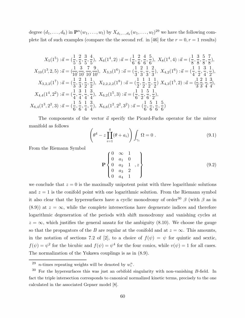
degree (d1, . . . , dk) in Pn(w1, . . . , wl) by Xd1,...,dk(w1, . . . , wl)

29 we have the following com-

plete list of such examples (compare the the second ref. in [46] for the r = 0, r = 1 results)

X5(15) :~a = (

1

5,2

5,3

5,4

5), X6(1

4, 2) :~a = (1

6,2

6,4

6,5

6), X8(1

4, 4) :~a = (1

8,3

8,5

8,7

8),

X10(13, 2, 5) :~a = (

1

10,3

10,

7

10,9

10), X3,3(1

6) :~a = (1

3,2

3,1

3,2

3), X4,2(1

6) :~a = (1

4,1

2,3

4,1

2),

X3,2,2(17) :~a = (

1

3,2

3,1

2,1

2), X2,2,2,2(1

8) :~a = (1

2,1

2,1

2,1

2) X4,3(1

5, 2) :~a = (1

3,2

3,1

4,3

4),

X4,4(14, 22) :~a = (

1

4,3

4,1

4,3

4), X6,2(1

5, 3) :~a = (1

6,1

2,5

6,1

2),

X6,4(13, 22, 3) :~a = (

1

6,5

6,1

4,3

4), X6,6(1

2, 22, 32) :~a = (1

6,5

6,1

6,5

6)

The components of the vector ~a specify the Picard-Fuchs operator for the mirror

manifold as follows (θ4 − z

4∏

i=1

(θ + ai)

)∫

γi

Ω = 0 . (9.1)

From the Riemann Symbol

P

0 ∞ 10 a1 00 a2 10 a3 20 a4 1

, z

(9.2)

we conclude that z = 0 is the maximally unipotent point with three logarithmic solutions

and z = 1 is the conifold point with one logarithmic solution. From the Riemann symbol

it also clear that the hypersurfaces have a cyclic monodromy of order30 β (with β as in

(8.9)) at z = ∞, while the complete intersections have degenerate indices and therefore

logarithmic degeneration of the periods with shift monodromy and vanishing cycles at

z = ∞, which justifies the general ansatz for the ambiguity (8.10). We choose the gauge

so that the propagators of the B are regular at the conifold and at z = ∞. This amounts,

in the notation of sections 7.2 of [2], to a choice of f(ψ) = ψ for quintic and sextic,

f(ψ) = ψ2 for the bicubic and f(ψ) = ψ4 for the four conics, while v(ψ) = 1 for all cases.

The normalization of the Yukawa couplings is as in (8.9).

29 n-times repeating weights will be denoted by wni .

30 For the hypersurfaces this was just an orbifold singularity with non-vanishing B-field. In

fact the triple intersection corresponds to canonical normalized kinetic terms, precisely to the one

calculated in the associated Gepner model [8].

60

9.2. Higher genus results on the quintic

We come now to the simplest compact Calabi-Yau, the zero locus of the quintic

5∑

i=1

x5i − 5ψ

5∏

i=1

xi = 0. (9.3)

in P4. The unique analytic solution at z = 0 is w0 =∑∞

n=05n!

(n!)5

(z55

)n, the three-point

coupling is as in (8.9). The rational and elliptic curves have been computed in [8][6].

d r = 0 1

1 2875 0

2 609250 0

3 317206375 609250

4 242467530000 3721431625

5 229305888887625 12129909700200

6 248249742118022000 31147299733286500

7 295091050570845659250 71578406022880761750

8 375632160937476603550000 154990541752961568418125

Table 10.a: The weighted sum of BPS states nrd for the quintic.

We agree with those results. Note however that the BPS numbers on the genus 1 cases differ

from the invariants defined in [6], where the maps from the torus to itself are subtracted

as explained in sec 3.3.

Unlike the non-compact cases, the reduction of the holomorphic anomaly involves a

global property of the model, the Euler number. The general form of F2 has been given

in [2]. In appendix B we give the complete result of the reduction of F331. In view of

the fast growing number of terms in Fr with the worldsheet genus r one may hope that

the ring of modular functions on the moduli space of the concrete Calabi-Yau – here

the quintic– transforming in L2−2r has a much lower dimension, so that there are many

relations between the terms in Fr. Restricting the expression given in appendix B for F3 to

the one-moduli case one has 50 terms of different functional form. Somewhat surprisingly

we find only one relation between the terms, which is reported in the Appendix B.

With these formulas we obtain the following genus r = 2, 3 results.

31 The F4, F5 expressions can be made available on request.

61

d r = 2 3 4

1 0 0 0

2 0 0 0

3 0 0 0

4 534750 8625 0

5 75478987900 −15663750 15520

6 871708139638250 3156446162875 −7845381850

7 5185462556617269625 111468926053022750 243680873841500

8 22516841063105917766750 1303464598408583455000 25509502355913526750

Table 10.b: The weighted sum of BPS states nrd for the quintic.

Note that for d > 7 the numbers of genus 2 invariants are expected to differ from the ones

given in [2], because of the different definition of the integer invariants related to F2.

Using the vanishing of n21 = n2

2 = n23 = 0, as explained below, we can fix the genus

2 ambiguity. Comparing (8.9) with (8.11) we learn that the distance to the singularity

t = (1 − z) = iµ/√α. Written in terms of µ it reads

f2 = − 571

36000+

83i

7200√

5µ−1 − 1

240µ−2 .

Note that the leading singularity confirms (8.11). Further the constant map contribution

is in accordance with [2][11].

To fix the genus 3 anomaly we used the vanishing of n21 = n2

2 = n23 = 0 and the fact

that n24 = (−1)2 · 3 · 2875 = 8625, as explained below. The number n3

5 turns out to be

negative, which is plausible as these curves come in singular families, but the actual value

has not been checked. Together with [11] for the constant map piece this determines

f3 =26857

126000000+

356921i

567000000√

5µ−1 − 5393

5040000µ−2 − 193i

50400√

5µ−3 +

1

1008µ−4 ,

i.e. the leading behavior is in perfect agreement with the c = 1 interpretation at the

conifold singularity. We note that the old definition of the invariant yielding n28 =

22516841063105918836250 seems incompatible with the BPS interpretation as it destroys

the integrality of the expansion of F3. The leading behavior of the ambiguity at genus 4 is

f4 = . . .+10001i

3024000√

5µ−5 − 1

1440µ−6

Most notably in order to get an integer expansion we had also to assume that there is also

a residue at ψ5 = 0 more precisely f4 ∼ 118530235187688859375 ψ−5.

62

We turn our attention to the application of (5.6) to verify some of the instanton

numbers that we have calculated for the quintic. Before we can do this, we have to

understand the restrictions on the degree and arithmetic genus of a curve in projective

space. This is part of the subject of Castelnuovo theory [47] [48]. Castelnuovo theory

gives the maximum arithmetic genus of a nondegenerate irreducible curve C of degree d

in Pr. Here, nondegenerate means that C is not contained in any hyperplane. This is not

a restriction, since any curve is nondegenerate inside the linear subspace that it spans.

We give a somewhat detailed description for P2, P3, and a general formula for Pr.

In P2, Castelnuovo theory is trivial, since a degree d curve necessarily has arithmetic

genus g = (d− 1)(d− 2)/2.

In P3, the result of [49] says that a nondegenerate curve of degree d either lies on a

quadric surface or else there is a number g(d) (to be described presently) such that any

curve in P3 has genus g ≤ g(d).

Note that a quadric surface is just P1×P1 so all possibilities for (d, g) can be computed

from the bidegrees (a, b) and d = a+ b, g = (a−1)(b−1). Some easy algebra shows that a

curve with degree and genus (d, g) can be found on a quadric precisely when (d− 2)2 − 4g

is a perfect square.

For g(d), we get

g(d) =d2 − 3d+ 6

6d ≡ 0(mod 3)

=d2 − 3d+ 2

6d 6≡ 0(mod 3)

(9.4)

For Pr, we give a less complete answer, and just note that the maximum genus possible

is found by writing

d− 1 = m(r − 1) + ǫ

with 0 ≤ ǫ < m. The formula is

g ≤(m

2

)(r − 1) +mǫ. (9.5)

If r = 3, it can be checked that the right hand side of (9.5) is the genus of a degree d curve

on a quadric, compare with Section 8.4.

Let’s apply these formulas to the quintic in low degree.

For d = 1, 2, it is clear that the only genus possible is 0. For d = 3, we can get g = 1

in the plane, and g = 0 is possible, even in P3 (e.g. bidegree (2, 1) in P1 × P1). Thus

ng1 = ng2 = 0 for g > 0 and ng2 = 0 for g > 1, consistent with Tables 10.a and 10.b.

63

Now d = 4 is more interesting. This is possible in P2 only for g = 3. In P3 it is either

on a quadric or g ≤ 1 by Castelnuovo theory. But we check immediately that g = 0, 1 are

the only possibilities on a quadric as well. Applying Castelnuovo theory to P4, we again

get g ≤ 1. So g = 2 is impossible on a quintic, and ng4 = 0 for g ≥ 4.

But this discussion does not mean that n24 vanishes. Quite the contrary, we can

apply (5.4) and (5.6) to the family of g = 3 curves, which are plane quartics. The plane

intersects the quintic in a quintic plane curve containing the quartic, leaving a residual

line. So we get the moduli space of these d = 4, g = 3 curves by taking a line on the

quintic, and passing all possible 2-planes through it, leaving a quartic over by reversing

the above reasoning. So the moduli space is 2875 copies of M = P2. In passing, we note

that n34 = 2875(3) = 8625 by (5.3). The universal curve C is a bit subtle. The projection

C → X (X is the quintic) is 1-1 except over the line (since a point of X not on the line

determines a unique 2-plane containing the line). But the fiber of this projection over the

line is a P1, so we must add 2 to the Euler characteristic of the CY (−200) to get the

Euler characteristic (−198) of C. Then the first equation in (5.4) together with (5.6) gives

for n24 the quantity 2875(−1)(−198+ (4)(3)) = 534750, as there are no reducible curves of

degree 4 in the plane. This is in agreement with Table 10.b.

We can similarly apply Castelnuovo theory to degree 5. Here the result is that plane

quintics have genus 6, and otherwise the genus is at most 2. The moduli space of plane

quintic curves is the same as the moduli space G = G(2, 4) of P2s in P4. By (5.3), we get

n65 = (−1)6e(G) = 10. We can also in principle get ng5 for 3 ≤ g ≤ 5 from (5.4) and (5.6).

Unfortunately, we don’t know how to compute the Euler characteristic of C(3), so we can

only compute ng5 for g = 4, 5 at present.

We can calculate e(C) as usual by considering the projection C → X . The fiber over

a point p ∈ X is identified with the set of 2 planes in P4 which contain p. This in turn

is identified with the Grassmannian G(1, 3) of lines in P3. So e(C) = e(X)e(G(1, 4)) =

−200 · 10 = −2000. Then the first equation in (5.4) together with (5.6) gives n55 =

(−1)5(−2000 + (2 · 3 − 2)10) = 1960.

The map C(2) → Hilb2X has fiber over Z ∈ Hilb2X the set of all 2 planes in P4

containing Z. Since Z is either a pair of distinct points or a single point of multiplicity 2

with a distinct tangent direction, we see that this fiber is isomorphic to P3 in either case.

64

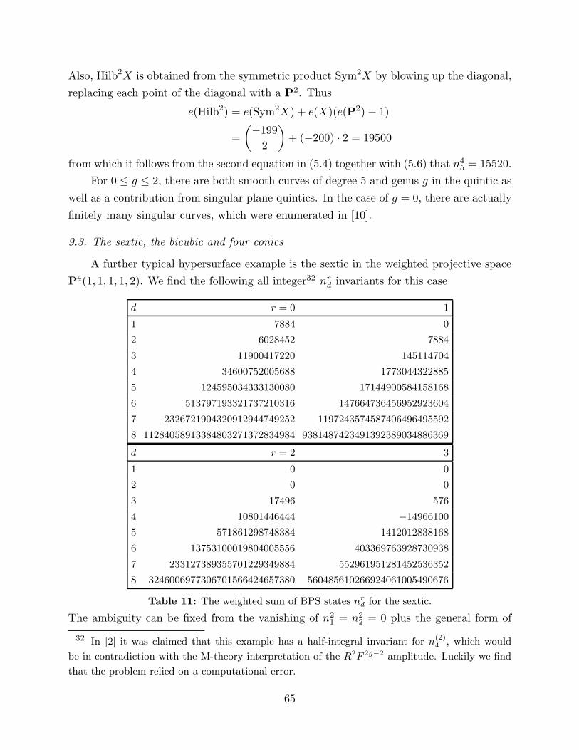
Also, Hilb2X is obtained from the symmetric product Sym2X by blowing up the diagonal,

replacing each point of the diagonal with a P2. Thus

e(Hilb2) = e(Sym2X) + e(X)(e(P2) − 1)

=

(−199

2

)+ (−200) · 2 = 19500

from which it follows from the second equation in (5.4) together with (5.6) that n45 = 15520.

For 0 ≤ g ≤ 2, there are both smooth curves of degree 5 and genus g in the quintic as

well as a contribution from singular plane quintics. In the case of g = 0, there are actually

finitely many singular curves, which were enumerated in [10].

9.3. The sextic, the bicubic and four conics

A further typical hypersurface example is the sextic in the weighted projective space

P4(1, 1, 1, 1, 2). We find the following all integer32 nrd invariants for this case

d r = 0 1

1 7884 0

2 6028452 7884

3 11900417220 145114704

4 34600752005688 1773044322885

5 124595034333130080 17144900584158168

6 513797193321737210316 147664736456952923604

7 2326721904320912944749252 1197243574587406496495592

8 11284058913384803271372834984 9381487423491392389034886369

d r = 2 3

1 0 0

2 0 0

3 17496 576

4 10801446444 −14966100

5 571861298748384 1412012838168

6 13753100019804005556 403369763928730938

7 233127389355701229349884 552961951281452536352

8 3246006977306701566424657380 560485610266924061005490676

Table 11: The weighted sum of BPS states nrd for the sextic.

The ambiguity can be fixed from the vanishing of n21 = n2

2 = 0 plus the general form of

32 In [2] it was claimed that this example has a half-integral invariant for n(2)4 , which would

be in contradiction with the M-theory interpretation of the R2F 2g−2 amplitude. Luckily we find

that the problem relied on a computational error.

65

the constant map contribution. Again we find the leading term of f2 in accordance with

(8.11) f2 = − 47325920 − 463

51840√

3µ−1 − 1

240µ−2.

For the genus 3 contribution we can fix a combination of n33, n

34 by demanding the

expected behavior of the µ−4 term in

f3 =3917

26127360+

61447i

117573120√

3µ−1 − 107945

94058496µ−2 − 25i

8064√

3µ−3 +

1

1008µ−4 .

This yields n34 = 36(−865581+781n3

3). The fact the µ−3 term is a relatively simple fraction

for other cases leads to the conjecture that the correct value is n33 = 576.

This can be checked by geometry as follows. Note that by projection to the first four

coordinates, X admits a 3 − 1 cover of P3. Writing the equation of the CY in the form

x35 + f4(x1, x2, x3, x4)x5 + f6(x1, x2, x3, x4) = 0

We see that the branch locus 4f34 + 27f2

6 has degree 12. A curve of degree 3 must either

map isomorphically to a degree 3 curve in P3 or be a triple cover of a line. Since degree 3

curves have genus at most 1, and we are interested in genus 3, we must have a triple cover

of a line branched at 4 points, which has genus 4. Thus M = G(1, 3), the Grassmannian

of P1s in P3. This has dimension 4 and Euler characteristic 6. So we already see that

n43 = 6.

We project the universal curve to X as usual; the fiber over p ∈ X is the set of

triple covers of lines which contain p, which is in 1-1 correspondence with the set of

lines in P3 which contain the image of p in P3. This is isomorphic to P2. We get

e(C) = e(P2)e(X) = 3(−204) = −612. Now an application of the first equation in (5.4)

and (5.6) gives (−1)3(−612 + 6 · 6) = 576.

We next consider as simplest complete intersection cases two cubics in P5, i.e. X3,3(16)

and four conics in P7, denoted X2,2,2,2(18).

d r = 0 1 2 3

1 1053 0 0 0

2 52812 0 0 0

3 6424326 3402 0 0

4 1139448384 5520393 0 0

5 249787892583 4820744484 5520393 0

6 62660964509532 3163476678678 23395810338 6852978

7 17256453900822009 1798399482469092 42200615912499 174007524240

8 5088842568426162960 944929890847710108 50349477671013600 785786604262830

Table 12: The weighted sum of BPS states nrd for the compl. intersection X3,3(1

6).

66

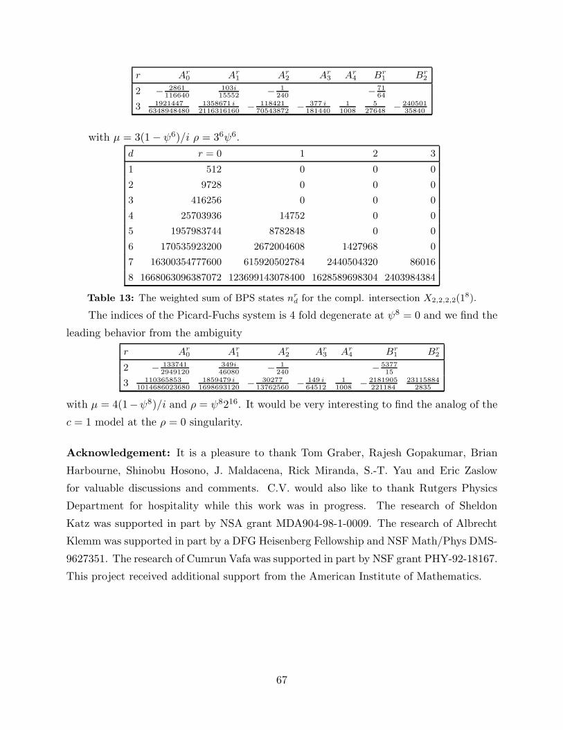
r Ar0 Ar

1 Ar2 Ar

3 Ar4 Br

1 Br2

2 − 2861116640

103i15552

− 1240

− 7164

3 19214476348948480

1358671 i2116316160

− 11842170543872

− 377 i181440

11008

527648

− 24050135840

with µ = 3(1 − ψ6)/i ρ = 36ψ6.

d r = 0 1 2 3

1 512 0 0 0

2 9728 0 0 0

3 416256 0 0 0

4 25703936 14752 0 0

5 1957983744 8782848 0 0

6 170535923200 2672004608 1427968 0

7 16300354777600 615920502784 2440504320 86016

8 1668063096387072 123699143078400 1628589698304 2403984384

Table 13: The weighted sum of BPS states nrd for the compl. intersection X2,2,2,2(1

8).

The indices of the Picard-Fuchs system is 4 fold degenerate at ψ8 = 0 and we find the

leading behavior from the ambiguity

r Ar0 Ar

1 Ar2 Ar

3 Ar4 Br

1 Br2

2 − 1337412949120

349i46080

− 1240

− 537715

3 1103658531014686023680

1859479 i1698693120

− 3027713762560

− 149 i64512

11008

− 2181905221184

231158842835

with µ = 4(1−ψ8)/i and ρ = ψ8216. It would be very interesting to find the analog of the

c = 1 model at the ρ = 0 singularity.

Acknowledgement: It is a pleasure to thank Tom Graber, Rajesh Gopakumar, Brian

Harbourne, Shinobu Hosono, J. Maldacena, Rick Miranda, S.-T. Yau and Eric Zaslow

for valuable discussions and comments. C.V. would also like to thank Rutgers Physics

Department for hospitality while this work was in progress. The research of Sheldon

Katz was supported in part by NSA grant MDA904-98-1-0009. The research of Albrecht

Klemm was supported in part by a DFG Heisenberg Fellowship and NSF Math/Phys DMS-

9627351. The research of Cumrun Vafa was supported in part by NSF grant PHY-92-18167.

This project received additional support from the American Institute of Mathematics.

67

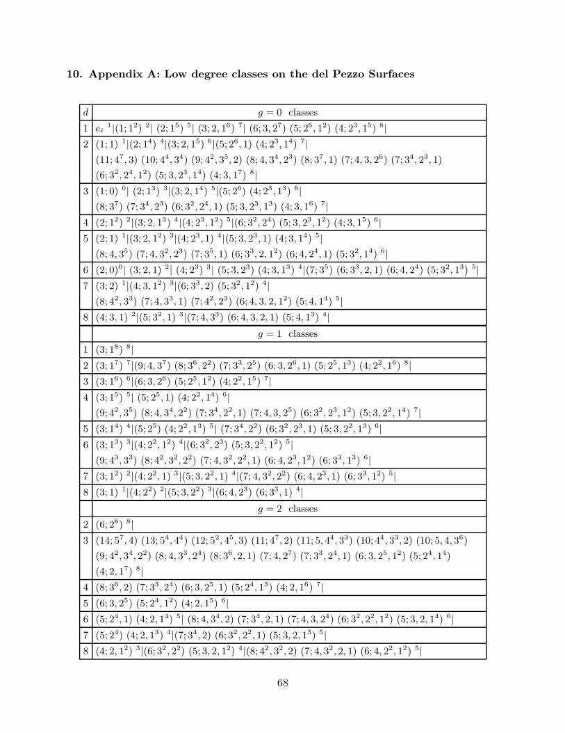
10. Appendix A: Low degree classes on the del Pezzo Surfaces

d g = 0 classes

1 ei1|(1; 12) 2| (2; 15) 5| (3; 2, 16) 7| (6; 3, 27) (5; 26, 12) (4; 23, 15) 8|

2 (1; 1) 1|(2; 14) 4|(3; 2, 15) 6|(5; 26, 1) (4; 23, 14) 7|

(11; 47, 3) (10; 44, 34) (9; 42, 35, 2) (8; 4, 34, 23) (8; 37, 1) (7; 4, 3, 26) (7; 34, 23, 1)

(6; 32, 24, 12) (5; 3, 23, 14) (4; 3, 17) 8|

3 (1; 0) 0| (2; 13) 3|(3; 2, 14) 5|(5; 26) (4; 23, 13) 6|

(8; 37) (7; 34, 23) (6; 32, 24, 1) (5; 3, 23, 13) (4; 3, 16) 7|

4 (2; 12) 2|(3; 2, 13) 4|(4; 23, 12) 5|(6; 32, 24) (5; 3, 23, 12) (4; 3, 15) 6|

5 (2; 1) 1|(3; 2, 12) 3|(4; 23, 1) 4|(5; 3, 23, 1) (4; 3, 14) 5|

(8; 4, 35) (7; 4, 32, 23) (7; 35, 1) (6; 33, 2, 12) (6; 4, 24, 1) (5; 32, 14) 6|

6 (2; 0)0| (3; 2, 1) 2| (4; 23) 3| (5; 3, 23) (4; 3, 13) 4|(7; 35) (6; 33, 2, 1) (6; 4, 24) (5; 32, 13) 5|

7 (3; 2) 1|(4; 3, 12) 3|(6; 33, 2) (5; 32, 12) 4|

(8; 42, 33) (7; 4, 33, 1) (7; 42, 23) (6; 4, 3, 2, 12) (5; 4, 14) 5|

8 (4; 3, 1) 2|(5; 32, 1) 3|(7; 4, 33) (6; 4, 3, 2, 1) (5; 4, 13) 4|

g = 1 classes

1 (3; 18) 8|

2 (3; 17) 7|(9; 4, 37) (8; 36, 22) (7; 33, 25) (6; 3, 26, 1) (5; 25, 13) (4; 22, 16) 8|

3 (3; 16) 6|(6; 3, 26) (5; 25, 12) (4; 22, 15) 7|

4 (3; 15) 5| (5; 25, 1) (4; 22, 14) 6|

(9; 42, 35) (8; 4, 34, 22) (7; 34, 22, 1) (7; 4, 3, 25) (6; 32, 23, 12) (5; 3, 22, 14) 7|

5 (3; 14) 4|(5; 25) (4; 22, 13) 5| (7; 34, 22) (6; 32, 23, 1) (5; 3, 22, 13) 6|

6 (3; 13) 3|(4; 22, 12) 4|(6; 32, 23) (5; 3, 22, 12) 5|

(9; 43, 33) (8; 42, 32, 22) (7; 4, 32, 22, 1) (6; 4, 23, 12) (6; 33, 13) 6|

7 (3; 12) 2|(4; 22, 1) 3|(5; 3, 22, 1) 4|(7; 4, 32, 22) (6; 4, 23, 1) (6; 33, 12) 5|

8 (3; 1) 1|(4; 22) 2|(5; 3, 22) 3|(6; 4, 23) (6; 33, 1) 4|

g = 2 classes

2 (6; 28) 8|

3 (14; 57, 4) (13; 54, 44) (12; 52, 45, 3) (11; 47, 2) (11; 5, 44, 33) (10; 44, 33, 2) (10; 5, 4, 36)

(9; 42, 34, 22) (8; 4, 33, 24) (8; 36, 2, 1) (7; 4, 27) (7; 33, 24, 1) (6; 3, 25, 12) (5; 24, 14)

(4; 2, 17) 8|

4 (8; 36, 2) (7; 33, 24) (6; 3, 25, 1) (5; 24, 13) (4; 2, 16) 7|

5 (6; 3, 25) (5; 24, 12) (4; 2, 15) 6|

6 (5; 24, 1) (4; 2, 14) 5| (8; 4, 34, 2) (7; 34, 2, 1) (7; 4, 3, 24) (6; 32, 22, 12) (5; 3, 2, 14) 6|

7 (5; 24) (4; 2, 13) 4|(7; 34, 2) (6; 32, 22, 1) (5; 3, 2, 13) 5|

8 (4; 2, 12) 3|(6; 32, 22) (5; 3, 2, 12) 4|(8; 42, 32, 2) (7; 4, 32, 2, 1) (6; 4, 22, 12) 5|

68

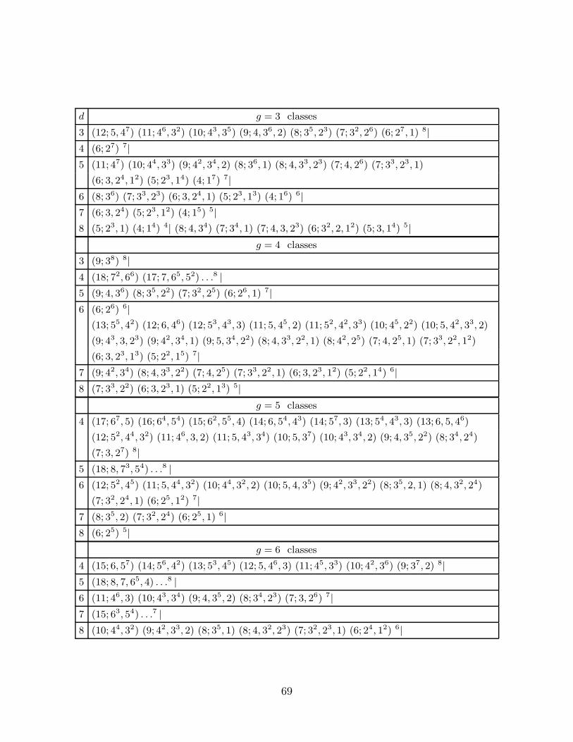
d g = 3 classes

3 (12; 5, 47) (11; 46, 32) (10; 43, 35) (9; 4, 36, 2) (8; 35, 23) (7; 32, 26) (6; 27, 1) 8|

4 (6; 27) 7|

5 (11; 47) (10; 44, 33) (9; 42, 34, 2) (8; 36, 1) (8; 4, 33, 23) (7; 4, 26) (7; 33, 23, 1)

(6; 3, 24, 12) (5; 23, 14) (4; 17) 7|

6 (8; 36) (7; 33, 23) (6; 3, 24, 1) (5; 23, 13) (4; 16) 6|

7 (6; 3, 24) (5; 23, 12) (4; 15) 5|

8 (5; 23, 1) (4; 14) 4| (8; 4, 34) (7; 34, 1) (7; 4, 3, 23) (6; 32, 2, 12) (5; 3, 14) 5|

g = 4 classes

3 (9; 38) 8|

4 (18; 72, 66) (17; 7, 65, 52) . . .8 |

5 (9; 4, 36) (8; 35, 22) (7; 32, 25) (6; 26, 1) 7|

6 (6; 26) 6|

(13; 55, 42) (12; 6, 46) (12; 53, 43, 3) (11; 5, 45, 2) (11; 52, 42, 33) (10; 45, 22) (10; 5, 42, 33, 2)

(9; 43, 3, 23) (9; 42, 34, 1) (9; 5, 34, 22) (8; 4, 33, 22, 1) (8; 42, 25) (7; 4, 25, 1) (7; 33, 22, 12)

(6; 3, 23, 13) (5; 22, 15) 7|

7 (9; 42, 34) (8; 4, 33, 22) (7; 4, 25) (7; 33, 22, 1) (6; 3, 23, 12) (5; 22, 14) 6|

8 (7; 33, 22) (6; 3, 23, 1) (5; 22, 13) 5|

g = 5 classes

4 (17; 67, 5) (16; 64, 54) (15; 62, 55, 4) (14; 6, 54, 43) (14; 57, 3) (13; 54, 43, 3) (13; 6, 5, 46)

(12; 52, 44, 32) (11; 46, 3, 2) (11; 5, 43, 34) (10; 5, 37) (10; 43, 34, 2) (9; 4, 35, 22) (8; 34, 24)

(7; 3, 27) 8|

5 (18; 8, 73, 54) . . .8 |

6 (12; 52, 45) (11; 5, 44, 32) (10; 44, 32, 2) (10; 5, 4, 35) (9; 42, 33, 22) (8; 35, 2, 1) (8; 4, 32, 24)

(7; 32, 24, 1) (6; 25, 12) 7|

7 (8; 35, 2) (7; 32, 24) (6; 25, 1) 6|

8 (6; 25) 5|

g = 6 classes

4 (15; 6, 57) (14; 56, 42) (13; 53, 45) (12; 5, 46, 3) (11; 45, 33) (10; 42, 36) (9; 37, 2) 8|

5 (18; 8, 7, 65, 4) . . .8 |

6 (11; 46, 3) (10; 43, 34) (9; 4, 35, 2) (8; 34, 23) (7; 3, 26) 7|

7 (15; 63, 54) . . .7 |

8 (10; 44, 32) (9; 42, 33, 2) (8; 35, 1) (8; 4, 32, 23) (7; 32, 23, 1) (6; 24, 12) 6|

69

11. Appendix B: B-model expression for Fg

The Fg can be determined by recursively solving the B-model anomaly equation [2].

As each contribution comes from the boundary of the moduli space of Riemann surfaces the

result has a graph interpretation in which each graph corresponds to a possible degeneration

of the genus g curve into components with lower genera. In the local case the descendent

of the dilaton decouples and only one sort of propagator Si,j occurs. They are in one

to one correspondence with the tubes connecting the irreducible components, in this way

each contribution of Fg corresponds precisely to one boundary stratum [7]. In the global

case one has three sorts of propagators shown below

-S -2 S ϕϕ-Si j iϕ

Propagors:

irreducible components:

g=0 g=1 g=2(1)

ϕ = ( 24 1 )−χ_F

The following Feynman rules hold for n,m = 0, 1, 2 . . .

F(0)ϕn = 0, F

(0)iϕn = 0, F

(0)ijϕn = 0, F

(g)i1,...im,ϕn+1 = (2g − 2 + n+m) = F

(g)i1,...im,ϕn

The graph contribution is divided by the following symmetry factors: k! for k equal

(self)links joining the same vertices, 2 for each selflink Sφ,φ, Si,i times the order of the

graph automorphism obtained by permuting the vertices. The generation of graphs pro-

ceeds along the line described for the the A-model in [7].

Twelve graphs contribute to F2, which were derived in [2]. Further we find that 193

graphs contribute to the free energy at genus 3. As it depends in an universal combinatorial

way on the lower genus boundary components, which also applies more generally to non-

topological string 3 loop calculations, and we have a powerfull check via integrality of the

BPS states on the quintic on its expression, we will give it below, despite its complicated

nature. Let χ = χ24

with χ the Euler number of the target space, F the genus 0 prepotential,

G = F1, H = F2 and Sij , Si, S the propagators of Kodaira-Spencer gravity [2] , then we

found

70

F3 = 2(1 + 2χ)HS + χ(1 + χ − 2χ2)S2 + 2GiHSi + (2 + χ)HiSi − 2χ(1 + 2χ)GiS Si−

1

2(2 + 3χ)GiGjS

iSj −1

2(2 + 3χ − χ2)GijS

iSj +1

6χ(2 + 3χ + χ2)FijkSiSjSk + GiHjS

ij+

1

2HijS

ij − (1 + 2χ)GiGjS Sij − (1 + 2χ)GijS Sij − GiGjGkSkSij − (2 + χ)GiGjkSkSij−

(1 + χ)GijkSkSij + χ(1 + 2χ)FijkS SkSij +1

4(2 + 3χ + χ2)FijklS

kSlSij −1

2GiGjklS

ilSjk+

1

2(2 + 3χ + χ2)FijkGlS

jSkSil − GiGjkSiSjk −1

2GiGjGklS

ilSjk + (1 +3

2χ)FijkGlS

kSlSij−

1

2FijkHlS

ilSjk + (1 + 2χ)FijkGlSSilSjk + FijkGlGmSmSilSjk + (1 +1

2χ)FijkGlmSmSilSjk+

(1 +1

2χ)FijklGmSlSimSjk −

1

4GijGklS

ikSjl + (1 +1

2χ)FijkGlGmSkSimSjl −

1

8GijklS

ijSkl+

(1 +1

2χ)FijkGlmSkSilSjm −

1

4(2 + 3χ + χ2)FijkFlmnSkSnSilSjm +

1

4(1 + 2χ)FijklS SijSkl+

1

8(2 + χ)FijklmSmSijSkl +

1

4FijklGmSmSijSkl +

1

4(1 + χ)FijkFlmnFpqrS

rSilSjpSknSmq+

1

8(2 + χ)FijkFlmnFpqrS

kSipSjnSlmSqr +1

4FijklGmnSimSjnSkl +

1

2FijkGlGmnSimSjnSkl+

1

6FijkGlmnSilSjmSkn −

1

6(1 + 2χ)FijkFlmnS SilSjmSkn −

1

6(1 + χ)FijkFlmnpSpSilSjmSkn−

1

6FijkFlmnGpSpSilSjmSkn −

1

2(2 + χ)FijkFlmnGpSnSilSjmSkp +

1

2FijkGlGmSkSijSlm+

1

16FijkFlmnFpqrsS

ijSksSlmSnpSqr −1

8(2 + 3χ)FijkFlmnSkSnSijSlm −

1

2FijkFlmnGpSnSipSjkSlm−

1

4(2 + 3χ + χ2)FijkFlmnSjSkSinSlm −

1

2(2 + χ)FijkFlmnGpSkSipSjnSlm +

1

8FijklmGnSijSknSlm−

1

16FijkFlmnFpqrFstuSisSjtSknSlpSmqSru +

1

4FijkGlmnSijSknSlm +

1

48FijklmnSijSklSmn−

1

4FijkFlmnGpSpSijSknSlm −

1

4(2 + χ)FijkFlmnpSpSijSknSlm +

1

12FijkFlmnFpqrsS

ipSjqSkrSlsSmn−

1

4FijkFlmnGpqS

ipSjqSknSlm −1

48FijklFmnpqS

imSjnSkpSlq −1

4(2 + χ)FijkFlmnpSkSilSjpSmn−

1

4(1 + 2χ)FijkFlmnS SijSknSlm −

1

4FijkFlmnpGqS

ilSjqSkpSmn −1

4FijkFlmnGpGqS

ipSjqSknSlm−

1

4FijkFlmnGpGqS

ilSjqSknSmp −1

4FijkFlmnGpqS

ilSjpSknSmq −1

12FijkFlmnpqS

ilSjmSkqSnp+

1

4FijkFlmnFpqrGsS

ipSjsSknSlqSmr +1

8FijkFlmnFpqrsS

ipSjqSknSlrSms +1

4FijklGmGnSimSjnSkl+

1

2FijkGlGmnSijSknSlm +

1

16FijkFlmnpqS

ijSkqSlmSnp −1

48FijkFlmnFpqrFstuSipSjsSknSlmSqrStu−

1

16FijklFmnpqS

ijSkmSlqSnp +1

4(2 + χ)FijkFlmnFpqrS

nSilSjmSkrSpq −1

6FijkFlmnpGqS

ilSjmSkpSnq+

1

12FijkFlmnFpqrS

rSilSjmSknSpq −1

4FijkFlmnpGqS

ijSklSmqSnp +1

8FijkFlmnFpqrGsS

ipSjsSknSlmSqr+

71

1

4FijkFlmnFpqrGsS

ilSjmSkrSnsSpq +1

8FijkFlmnFpqrS

rSijSknSlmSpq +1

6FijkGlGmGnSimSjnSkl+

1

8FijkFlmnFpqrsS

ilSjpSksSmnSqr +1

8FijkFlmnFpqrsS

ilSjmSksSnpSqr +1

2FijkGlmSkSijSlm−

1

8FijkFlmnpSkSijSlmSnp −

1

24FijkFlmnFpqrFstuSipSjsSknSlqSmtSru −

1

8FijkFlmnGpqS

ijSkqSlmSnp−

FijkHSkSij −1

16FijkFlmnFpqrFstuSilSjmSkrSnsSpqStu −

1

8FijkFlmnFpqrFstuSilSjpSkuSmqSnrSst

4780 graphs contribute to F4, which starts with

F4 =S3

248832(χ− 24)χ(1728 + 168χ+ 5χ2) + . . .

This first term comes from the graphs

1

1

1 1 1

1 1

1 1 1

1

4 2 3!

2 3! 8 4

8

8 3!

2 23!

The contributions of the remaining graphs have been calculated and used to evaluate

the generating function for the genus 4 curves on the quintic see Table 10. 172631 graphs

contribute to F5. These data are available on request.

We finally report a “Ward-identity” between the correlators at genus 3 on the quintic.

(Sψψ)4(134560SΨF 3ψψψ − 7305(Sψψ)2 − 8139F 2

ψψψψ + 3364FψψψFψψψψψ−

3372FψψψFψψψψGψ + 1440F 2ψψψG

2ψ − 4SψψF 2

ψψψ(2877FψψψGψ − 1697Fψψψψ)+

20184F 2ψψψGψψ) = 0.

72

References

[1] R. Gopakumar and C. Vafa, “M-theory and Topological Strings-I & II,” hep-

th/9809187, hep-th/9812127.

[2] M. Bershadsky, S. Cecotti, H. Ooguri, and C. Vafa, “Kodaira-Spencer Theory of Grav-

ity and Exact Results for Quantum String Amplitudes,” Commun. Math. Phys. 165

(1994) 311-428.

[3] I. Antoniadis, E. Gava, K.S. Narain, T.R. Taylor, “Topological amplitudes in String

Theory” , Nucl. Phys. B413 (1994) 162, hep-th/9307158, I. Antoniadis, E. Gava,

K. S. Narain, “Moduli Corrections to gravitational Couplings from Sring Loops”,

Phys. Lett. B238 (1992) 209, hep-th/9203071 and “Moduli Corrections to Gauge and

gravitational Couplings in four-dimensional Superstrings”, Nucl. Phys. B383 (1992)

93, hep-th/9204030.

[4] I. Antoniadis, E. Gava, K. S. Narain and T. R. Taylor, Nucl. Phys. B455 (1995) 109,

hep-th/9507115.

[5] D.A. Cox and S. Katz, Mirror Symmetry and Algebraic Geometry, Mathematical

Surveys and Monographs vol. 68, Amer. Math. Soc., Providence, RI 1999.

[6] M. Bershadsky, S. Cecotti, H. Ooguri, and C. Vafa, “Holomorphic Anomalies in Topo-

logical Field Theories,” Nucl. Phys. B405 (1993) 279.

[7] A. Klemm and E. Zaslow, “Local Mirror Symmetry at Higher Genus”, hep-th/9906046.

[8] P. Candelas, X. C. De La Ossa, P. Green, and L Parkes, “A Pair of C-Y Manifolds as

an Exactly Soluble Superconformal Theory,” Nucl. Phys. B359 (1991) 21–74.

[9] P. Aspinwall and D. Morrison, “Topological Field Theory and Rational Curves,”

Comm. Math. Phys. 51 (1993)245, Yu. I. Manin, “Generating Functions in Alge-

braic Geometry and Sums over Trees” in “The moduli space of curves” (Texel Island,

1994), Progr. Math. 129, Birkhauser, Boston (1995) 401–417; alg-geom/9407005, C.

Voisin, A Mathematical Proof of a formula of Aspinwall and Morrison, Comp. Math.

104 (1996) 135 .

[10] I. Vainsencher, Enumeration of n-fold tangent hyperplanes to a surface, J. Algebraic

Geom. 4, 1995, 503–526, alg-geom/9312012

[11] C. Faber and R. Pandharipande, Hodge Integrals and Gromov-Witten Theory,

math.AG/9810173.

[12] E. Witten, “Two-dimensional Gravity and Intersection Theory on Moduli Space,”

Surveys in Differential Geometry 1 (1991) 243-310.

[13] M. Kontsevich, “Intersection theory on the moduli space of curves and the matrix

Airy function”, Comm. Math. Phys. 147 (1992) 1-23 .

[14] C. Faber, “Algorithm for Computing Intersection Numbers on Moduli Spaces

of Curves, with an Application to the Class of the Locus of the Jacobians,”

math.AG/9706006.

73

[15] S. Katz, D.R. Morrison, and M.R. Plesser, Nucl. Phys. B477 (1996) 105, hep-

th/9601108.

[16] A. Lawrence and N. Nekrasov,“Instanton sums and five-dimensional Gauge Theories”,

Nucl. Phys. B513 (1998) 239, hep-th/9706025.

[17] P. Griffiths and J. Harris, Principles of Algebraic Geometry , Wiley-Interscience, New

York 1978.

[18] S.-T. Yau and E. Zaslow, “BPS States, String Duality, and Nodal Curves on K3,”

Nucl. Phys. B471 (1996) 503-512; hep-th/9512121.

[19] J. Bryan, N.C. Leung, S. Katz, in preparation.

[20] A. Beauville, Duke Math. J. 97 (1999) 99–108.

[21] W. Lerche and S. Stieberger, “1/4 BPS States and Non-Perturbative Couplings in

N=4 String Theories”, hep-th/9907133 .

[22] E. Witten, “String Theory Dynamics in Various Dimensions”, Nucl. Phys.B443 (1995)

85, hep-th/9503124.

[23] S. Hosono, M.-H. Saito, and A. Takahashi, “Holomorphic Anomaly Equation and BPS

State Counting of Rational Elliptic Surface,” hep-th/9901151.

[24] M. Marino and G. Moore, “Counting higher genus curves in a Calabi-Yau Manifold,”

Nucl. Phys. B543 (1999) 592, hep-th/9808131.

[25] M. Berschadsky, V. Sadov and C. Vafa, “D-Branes and Toplological Field Theories”,

Nucl. Phys. B463 (1996) 420, hep-th/9511222 and C. Vafa, “Lectures on Strings and

Dualities”, hep-th/9702201.

[26] L. Gottsche, Math. Ann.286 (1990) 193

[27] J. Bryan, N.C. Leung, “The enumerative geometry of K3 surfaces and modular forms,”

alg-geom/971103 .

[28] A. Strominger and C. Vafa, “Microscopic Origin of the Bekenstein-Hawking Entropy,”

Phys. Lett. B379 (1996) 99, hep-th/9601029.

[29] J.C. Breckenridge, R.C. Myers, A.W. Peet, C. Vafa, “D-Branes and Spinning Black

Holes”, Phys. Lett. B391 (1997) 93, hep-th/9602065.

[30] R. Dijkgraaf, G. Moore, E. Verlinde and H. Verlinde, “Elliptic Genus of Symmetric

Products and Second quantized Strings”, Commun. Math. Phys. 185 (1997) 197-209,

hep-th/9608096.

[31] A. Altman and S. Kleiman, “Foundations of the theory of Fano schemes”, Comp.

Math. 34 (1977) 3.

[32] S. Katz and S.A. Strømme, Schubert, a Maple package for intersection theory in

algebraic geometry, http://www.math.okstate.edu/˜katz/schubert.html .

[33] C. Vafa, Black Holes and Calabi-Yau Threefolds”, Adv. Theor. Math. Phys. 2 (1998)

207, hep-th/9711067.

[34] T.-M. Chiang, A. Klemm, S.-T. Yau, and E. Zaslow, “Local Mirror Symmetry: Cal-

culations and Interpretations,” hep-th/9903053.

74

[35] M. Kontsevich and Y. Manin, “Gromov-Witten classes, Quantum Cohomology and

enumerative Geometry”, Commun. Math. Phys. 164 (1994) 525–562; hep-th/9402147,

P. Di Francesco and C. Itzykson, “Quantum intersections rings”, hep-th/9412175, C.

Itzykson, “Counting Rational Curves on Rational Surfaces”, Int. J. Mod. Phys. B8

(1994) 3703–3724

[36] N. Nekrasov, “In the Woods of M-theory”, hep-th/9810168.

[37] B. Harbourne, “Rational surfaces with K2 > 0”, Proc. AMS 124 (1996) 727–733.

[38] S. Katz, A. Klemm and C. Vafa, “Geometric Engineering of quantum Field Theories,”

Nucl.Phys. B497 (1997) 173-195, hep-th/9609239.

[39] J.A. Minahan, D. Nemechansky and N.P. Warner, “Partition function for the BPS

States of the Non-Critical E8 String,” Adv. Theor. Math.Phys. 1 (1998) 167-183; hep-

th/9707149, J.A. Minahan, D. Nemechansky, C. Vafa and N.P. Warner, “E-Strings

and N = 4 Topological Yang-Mills Theories,” Nucl. Phys. B527 (1998) 581-623.

[40] M. Kontsevich, “Enumeration of Rational Curves via Torus Actions,” in The Mod-

uli Space of Curves, Dijkgraaf et al eds., Progress in Mathematics 129, Birkhauser

(Boston) 1995, A. Givental, “A Mirror Theorem for Toric Complete Intersections,”

Topological Field Theory, Primitive Forms and Related Topics (Kyoto,1996), Prog.

Math. 160, 141-175; math.AG/9701016, B. Lian, K. Liu, and S.-T. Yau, “Mirror

Principle I& II,” Asian J. of Math. Vol. 1 (1997) 729-763; math.AG/9712011 &

math.AG/9905006.

[41] A. Erdelyi, W. Magnus, F. Oberhettinger, F. Tricomi, “The Bateman Project: Higher

Transcendental Functions, V ol.1.

[42] A. Klemm, P. Mayr, and C. Vafa, “BPS States of Exceptional Non-Critical Strings,”

Nucl. Phys. B58 (Proc. Suppl.) (1997) 177-194; hep-th/9607139.

[43] W. Lerche, P. Mayr, N.P. Warner, Nucl.Phys. B499 (1997) 125–148.

[44] D. Ghoshal and C. Vafa, “c=1 String as the Topological Theory of the Conifold,”

Nucl. Phys. B453 (1995) 121.

[45] R. Gopakumar and C. Vafa, “Topological Gravity as Large N Topological Gauge

Theory”, Adv. Theor. Math. Phys. 2 (1998) 413-442, hep-th/9802016.

[46] S. Hosono, A. Klemm, S. Theisen and S.T. Yau, “Mirror Symmetry, Mirror Map and

Applications to Calabi-Yau Hypersurfaces,” Comm. Math. Phys. 167 (1995)301–350,

hep-th/9308122; and “Mirror Symmetry, Mirror Map and Applications to Calabi-Yau

Hypersurfaces,” Nucl. Phys. B433 (1995) 501-554, hep-th/9406055.

[47] R. Hartshorne, Algebraic Geometry , Springer-Verlag, Berlin 1977.

[48] J. Harris, Curves in Projective Space, University of Montreal Press, 1982.

[49] L. Gruson and C. Peskine, “Genre des courbes de l’espace projectif, II”, Ann. Sci.

ENS 15 (1982) 401–418.

75