arX

iv:a

stro

-ph/

9909

359v

1 2

1 Se

p 19

99Draft version July 12, 2011

Preprint typeset using LATEX style emulateapj

THERMAL INSTABILITY AND PHOTOIONIZED X-RAY REFLECTION IN ACCRETION DISKS

Sergei Nayakshin1, Demosthenes Kazanas and Timothy R. Kallman

Laboratory for High Energy Astrophysics, NASA/Goddard Space Flight Center, Code 661, Greenbelt, MD, 20771

Draft version July 12, 2011

ABSTRACT

We study the illumination of accretion disks in the vicinity of compact objects by an overlying X-raysource. Our approach differs from previous works of the subject in that we relax the simplifying assump-tion of constant gas density used in these studies; instead we determine the density from hydrostaticbalance which is solved simultaneously with the ionization balance and the radiative transfer in a plane-parallel geometry. We calculate the temperature profile of the illuminated layer and the reprocessedX-ray spectra for a range of physical conditions, values of photon index Γ for the illuminating radiation,and the incident and viewing angles.

In accordance with some earlier studies, we find that the self-consistent density determination makesevident the presence of a thermal ionization instability well known in the context of quasar emission linestudies. The main effect of this instability is to prevent the illuminated gas from attaining temperaturesat which the gas is unstable to thermal perturbations. Thus, in sharp contrast to the constant densitycalculations that predict a continuous and rather smooth variation of the gas temperature in the illu-minated material, we find that the temperature profile consists of several well defined thermally stablelayers. Transitions between these stable layers are very sharp and can be treated as discontinuities as faras the reprocessed spectra are concerned. In particular, the uppermost layers of the X-ray illuminatedgas are found to be almost completely ionized and at the local Compton temperature (∼ 107 − 108 K);at larger depths, the gas temperature drops abruptly to form a thin layer with T ∼ 106 K, while at yetlarger depths it decreases sharply to the disk effective temperature. For a given X-ray spectral index,this discontinuous temperature structure is governed by just one parameter, A, which characterizes thestrength of the gravitational force relative to the incident X-ray flux.

We find that most of the Fe Kα line emission and absorption edge are produced in the coolest, deepestlayers, while the Fe atoms in the hottest, uppermost layers are generally almost fully ionized, hencemaking a negligible contribution to reprocessing features in ∼ 6.4 − 10 keV energy range. We also findthat the Thomson depth of the top hot layers is pivotal in determining the fraction of the X-ray fluxwhich penetrates to the deeper cooler layers, thereby affecting directly the strength of the Fe line, edgeand reflection features. Due to the interplay of these effects, for Γ <∼ 2, the equivalent width (EW) of theFe features decreases monotonically with the magnitude of the illuminating flux, while the line centroidenergy remains at 6.4 keV. We provide a summary of the dependence of the reprocessing features in theX-ray reflected spectra on the gravity parameter A, the spectral index Γ and other parameters of theproblem.

We emphasis that the results of our self-consistent calculations are both quantitatively and qualita-tively different from those obtained using the constant density assumption. Therefore, we propose thatfuture X-ray reflection calculations should always utilize hydrostatic balance in order to provide a reliableinterpretation of X-ray spectra of AGN and GBHCs.

Subject headings: accretion, accretion disks —radiative transfer — line: formation — X-rays: general —radiation mechanisms: non-thermal

1. INTRODUCTION

The importance of X-ray reflection off the surface ofcold matter in the spectra of accreting compact objectshas been recognized for a long time. Basko, Sunyaev &Titarchuk (1974) discussed the reprocessing of X-rays froman accreting neutron star incident on the surface of theadjacent cooler companion, while Guilbert & Rees (1988)considered such reprocessing in “clouds” of cold matterin the vicinity of AGN. Lightman & White (1988) stud-ied similar reprocessing on the surface of a geometricallythin, optically thick accretion disk, placing the problemwithin the “standard” paradigm for AGN and GalacticBlack Hole Candidates (GBHC) which asserts the pres-

ence of such disks illuminated by an overlying hot corona(e.g., Liang & Price 1977; Galeev, Rosner & Vaiana 1979;Haardt, Maraschi & Ghisellini 1994). The consequences ofX-ray reprocessing in this specific geometry (arrangement)have been explored in detail theoretically and observation-ally.

Lightman & White (1988) and White, Lightman &Zdziarski (1988) computed the Green’s function for theangle-averaged reflected spectrum assuming that the illu-minated material is cold, non-ionized, and has a fixed gasdensity. Soon thereafter, a number of authors includedthe effects of ionization on the structure of the iron linesand the reflected continuum (e.g., George & Fabian 1991;

1National Research Council Associate

1

2

Turner et al. 1992). Krolik, Madau & Zycki(1994) calcu-lated the X-ray reflection and the iron lines from a puta-tive distant obscuring torus, while Magdziarz & Zdziarski(1995) calculated angle-dependent reflection componentoff cold matter; Poutanen, Nagendra & Svensson (1996)included polarization in their calculations of the reflectedspectra off neutral matter and Blackman (1999) enunci-ated the influence of the possible concave geometry of thedisk on the iron line profile.

To date, the most careful (in terms of the ionizationphysics) calculations of the X-ray reflection componentand the iron lines from ionized accretion disks in AGNare probably those of Ross and Fabian (1993), Matt et

al. (1993), Zyckiet al. (1994), and more recently for GB-HCs of Ross, Fabian & Brandt (1997) and Ross, Fabian &Young (1999). All these studies made use of a simplifyingassumption, namely that the density in the illuminatedgas be constant and equal to the disk mid-plane value.The justification for this assumption was the fact thatin the simplest version of radiation-dominated Shakura-Sunyaev disks (Shakura & Sunyaev 1973, hereafter SS73,see their §2a), thought to be the case in the majority ofthe observed sources, the gas density is roughly constantin the vertical direction. Note that the accretion diskis radiation-dominated as long as dimensionless accretionrate, m ≡ ηMc2/LEdd ≡ L/LEdd (LEdd is the Edding-ton accretion rate, L is the disk bolometric luminosity,η = 0.06 is the radiative efficiency of the standard disk inNewtonian limit), is greater than about ∼ 5 × 10−3.

Recently, Ross, Fabian & Young (1999) suggested thatthe vertical density structure may follow a Gaussian lawwith the vertical coordinate z (ρ(z) = ρ(0) exp[−(z/z0)

2],where z0 is the scale height, and ρ(0) is the central diskdensity). They showed that weakness of the observed Fefeatures in spectra of some GBHCs could be interpreted asa result of high degree of ionization of the exposed gas, asopposed to the cold matter intercepting a smaller fractionof the emitted X-rays thereby preserving the paradigm ofa cold disk with an overlying hot corona2.

However, a self-consistent approach requires that the gasdensity be determined from the condition of hydrostaticequilibrium solved simultaneously with ionization, energybalance and radiation transfer equations rather than beassumed. As such, the approximation of the constant gasdensity was made by Shakura & Sunyaev (1973) for disksheated by viscous dissipation and for large optical depthsonly. Therefore, even though the disks we will be consid-ering may be radiation dominated, the constant densityassumption may apply only to their deep “cooler” layers,where the X-ray heating is negligible. On the contrary,in the upper disk layers, this heating exceeds the viscousheating by orders of magnitude (see §3.2), and thus theconstant density approximation of SS73 cannot be simplyextended to these layers. Further, a self-consistent densitydetermination is especially important because of the ex-istence of a thermal instability that allows (and requiresunder some conditions!) illuminated adjacent gas regionsto have vastly different densities and temperatures but,by necessity, similar pressure (see Krolik, McKee & Tarter1981 – hereafter KMT; Raymond 1993; Ko & Kallman1994; Rozanska& Czerny 1996, and Rozanska1999). For

example, when the gas pressure in the illuminated atmo-sphere falls below a fraction of the incident X-ray radiationpressure Fx/c (Fx is the incident flux), the gas tempera-ture may jump from low values (of the order ∼ 105 Kelvinfor AGN) to the Compton temperature, which is typicallyas large as ∼ 107 − 108 K. This large jump in tempera-ture makes it impossible to approximate the gas density byeither a constant or Gaussian profile, as we will see below.

In this paper, we present an X-ray reprocessing calcu-lation that matches or exceeds the most detailed previousworks in terms of the radiation transfer and ionization bal-ance calculations, but also relaxes the assumption of theconstant gas density. We adopt a plane-parallel geome-try and gravity law appropriate for the standard geomet-rically thin SS73 disk, and solve for the gas density viahydrostatic pressure equilibrium, taking into account thepressure force due to the X-radiation as well.

The structure of the paper is as follows: In §2 we presentgeneral considerations on how the thermal instability mayinfluence the X-ray reprocessing and review previouslyknown results. In §3 we describe the numerical methodswe use to solve the radiation transfer, ionization, energy,and hydrostatic balance equations. Readers not interestedin these details may skip the latter section and proceed to§4, where we show several representative tests and com-pare our results with those obtained with the usual con-stant density assumption. Radiation-dominated disks arediscussed in §5. Complications arising due to possible X-ray driven gas evaporation in the case of accretion diskswith magnetic flares are discussed briefly in §6. We sum-marize our results and give our conclusions in §7. TheAppendix contains notes on the importance of the thermalconduction, two-phase cloudy structure and the intrinsicdisk viscous dissipation for the given problem.

2. THERMAL IONIZATION INSTABILITY AND X-RAYREFLECTION

In order to simplify our treatment we will assume inwhat follows that the geometry of the X-ray illuminatedgas is a plane parallel one, i.e., the vertical z-coordinate isthe only dimension relevant to the problem. The surface ofthe accretion disk is illuminated by X-rays with a power-law plus exponential roll-over spectrum (the power law in-dex, Γ = 1.5− 2.4, the cutoff energy is fixed at Ecut = 200keV). Note that due to the fact that most of this radiationis thermalized in the disk and consequently re-radiated,the ionizing spectrum consists, in the zeroth approxima-tion, of the incident X-ray spectrum plus the reprocessedblack-body radiation with an equal amount of flux. Thevertical coordinate z is counted from the disk mid-plane.The optical depth in the reflecting material is measuredfrom the top of the illuminated layer, i.e., τ(z = zt) = 0,where zt is the vertical coordinate of the reflector’s top, tobe found in a full self-consistent calculation.

The existence of multiple temperature solutions for anX-ray illuminated gas at a given pressure was shown byBuff & McCray (1974) and then elaborated by KMT. Itwas noted that some of these solutions are unstable. Thisinstability conforms to the criterion for thermal instabil-ity discovered by Field (1965). He argued that a physicalsystem is usually in pressure equilibrium with its surround-

2Similar suggestions were made earlier in an unpublished paper by Nayakshin & Melia (1997c), and in Nayakshin (1998a,b).

3

ings. Thus, any perturbations of the temperature T andthe density n of the system should occur at a constantpressure. The system is unstable when

(

∂Λnet

∂T

)

P

< 0, (1)

where P is the full gas pressure, and the “cooling func-tion,” Λnet, is the difference between cooling and heat-ing rates per unit volume (divided by the gas density nsquared).

In ionization balance studies, it is convenient to definethe “density ionization parameter” ξ, equal to (e.g., KMT)

ξ =4πFx

nH, (2)

where nH is the hydrogen density. For situations in whichthe pressure rather than the gas density is of physical im-portance one defines the “pressure ionization parameter”as

Ξ ≡ Fx

cPgas

, (3)

where Pgas is the full gas pressure due to neutral atoms,ions and electrons (we neglect the trapped line radiationpressure in this paper). KMT showed that the instabilitycriterion (1) is equivalent to

(

dΞ

dT

)

Λnet=0

< 0 , (4)

where the derivative is taken with the condition Λnet = 0satisfied, i.e., when the energy and ionization balances areimposed. In this form, the instability can be readily seenwhen one plots temperature T versus Ξ, since the unstableparts of the curve are the ones that have a negative slope.

In Figure (1), we show several illustrative ionizationequilibrium curves for the case with the ionizing X-ray fluxFx = 1016 erg sec−1 cm−2, photon spectral index Γ = 1.9and an equal amount of the black-body flux with temper-ature equal to the effective temperature for the given Fx,i.e., kT = kTeff ≃ 10 eV. Since these curves produce ashape somewhat similar to the letter “S”, they are com-monly referred to as “S-curves”. The solid curve shown inFigure (1) was computed assuming that all resonant linesare optically thin, and we will concentrate on this casefor now (significance of the other curves in Fig. 1 will beexplained in §3.6). One can see that equilibria in temper-ature range kT ∼ 20 − 90 eV and kT ∼ 150 − 103 eVare unstable. It is also worthwhile pointing out that theinstability criterion (eq. [4]) can be shown to be equiv-alent to c2

s = dPgas/dρ < 0, where ρ is the gas densityand cs is the sound speed (see Nayakshin 1998c, §4.5.) Animaginary value of the sound speed in the regions with thenegative slope of the ionization balance curve is clearly an“unusual” situation, a fact that perhaps helps to clarifythe existence of the thermal instability.

A number of authors have investigated the structure ofX-ray illuminated atmospheres in the case of a star in abinary system (e.g., Alme & Wilson 1974; Basko et al.1974; McCray & Hatchett 1975; Basko et al. 1977; Lon-don, McCray, & Auer 1981). These authors concluded

that, as one moves from the star’s interior to the atmo-sphere (that is from Ξ ≪ 1 to Ξ = ∞), the gas temper-ature first follows the S-curve until point (a) [cf. Fig. 1]is reached. For Ξ > Ξ(a), the photo-ionization heatingexceeds the cooling and no equilibrium is possible untilthe gas heats up to a fraction of the Compton tempera-ture, kTc

>∼ 1 keV, where even the high-Z elements becomenearly completely ionized. At this state, the gas coolingand heating is effected predominantly by Compton heatingand Compton and bremsstrahlung cooling (KMT). Thetransition from point (a) to point (b) is very sharp3. Infact, since in the case of a star the escape energy for a pro-ton is around Ees ∼ 100eV , and the Compton temperaturekTc ∼ few keV ≫ Ees, a strong wind results. McCray &Hatchett (1975) treated the temperature discontinuity asa deflagration wave, in which case the gas pressure is alsodiscontinuous across the (a-b) boundary; it is the momen-tum flux that is continuous across the transition.

We are primarily interested in the inner part of an ac-cretion disk, where most of the X-rays are produced andwhere most of the X-ray reprocessing features presumablyarise. Because the gas Compton temperature, Tc

<∼ 108 K,is smaller than the virial temperature in the inner disk byseveral orders of magnitude, no thermally driven wind willescape from the system, and thus there should be a staticconfiguration for the X-ray heated layer in this region (seeBegelman, McKee & Shields 1983). Thus, the problem offinding the gas density is reduced to finding its hydrostaticequilibrium configuration.

Raymond (1993) and Ko & Kallman (1994) have cal-culated the structure of the accretion disk atmospheresaround LMXBs at large radii with special attention tothe unknown origin of the UV and soft X-ray emissionlines. The illuminating spectrum was assumed to be ther-mal bremsstrahlung with T = 108 K. The work of theseauthors was pioneering in that they calculated the den-sity of the illuminated gas using hydrostatic balance, thustaking the thermal instability into account consistently.Rozanska& Czerny (1996), Rozanska(1999) considered thestructure of X-ray illuminated disk atmospheres in AGN,including the effects of thermal conduction. The radiationtransfer methods used by these last authors did not allowthem to study the effects of spectral reprocessing in detail.

Our paper is a natural extension of the work of these au-thors. Since we study accretion disks in Seyfert 1 Galaxiesand GBHCs rather than in LMXBs as did Raymond (1993)and Ko & Kallman (1994), we use the ionizing spectrumtypical for Seyfert 1 Galaxies and GBHCs and deal withthe innermost part of the accretion disk. Compared withwork of Rozanska& Czerny (1996) and Rozanska(1999),we solve the radiation transfer “exactly” by using the ex-act frequency dependent cross sections and the variableEddington factor method to take into account anisotropyof the radiation field.

3. THE NUMERICAL APPROACH

3.1. Radiation Transfer

Here we describe the part of our code that performs theradiation transfer. The incident X-rays come with a givenspecific intensity Ix(E, µ), where E is the photon energyand µ is the cosine of the angle that the given direction

3The line cooling complicates this situation; we will come back to this question in §3.6

4

makes with the normal to the surface of the disk (notethat Ix(E, µ) is the intensity already integrated over theazimuthal angle, i.e., it is 2π times the usual radiation in-tensity). The X-ray intensity is normalized in such a wayas to give the total X-ray flux incident on the reflector, Fx

(erg cm−2 sec−1), integrated over all photon energies andall incident angles:

Fx =

∫ 0

−1

|µ| dµ

∫ ∞

0

dE Ix(E, µ) . (5)

We limit ourselves to treating only τmax = 4 upper Thom-son depths of the illuminated layers, since it is both suf-ficient and practical (see §3.2). We break the reflectinglayer into Nz (typically a few hundred) individual bins.The binning is the finest around the discontinuity in thegas temperature and density.

The ultimate goal of the radiation transfer is to find thephoton intensity, I(E, µ, τt) as a function of photon energyE, angle (or µ) and position (equivalently τt) everywherein the slab. Luckily, the ionization balance part of the cal-culations only depends on the intensity integrated over allangles, J(E, τt):

J(E, τt) =

∫ +1

−1

dµI(E, µ, τt) , (6)

which then allows us to use the variable Eddington fac-tors method (see Mihalas 1978, §6.3). The variable Ed-dington factors g(E, τt) are defined as the ratio of thesecond to the zeroth moment of the photon intensity:g(E, τt) ≡ K(E, τt)/J(E, τt), where K(E, τt) is given byan equation analogous to Equation (6), but with the ad-ditional factor of µ2 in the integral. Mihalas (1978) showsthat the transfer equation then reduces to

∂2

∂τ2[g(E, τt)J(E, τt)] = J − S , (7)

where S(E, τt) is the source function, defined as

S(E, τt) ≡αs

αs + αaCJ(E, τt) +

1

αs + αaj(E, τt) , (8)

where αs and αa are the scattering and absorption coef-ficients, respectively: αs = neσkn(E), where ne = 1.2nH

is the electron density, σkn(E) is the Klein-Nishina crosssection; αa = nHσa(E), where nH is the hydrogen densityand σa(E) is the continuum absorption cross section cal-culated by XSTAR (Kallman & McCray 1982; Kallman& Krolik 1986). Further, dτ in Equation (7) is a differ-ential of the total optical depth, so that it is a functionof both photon energy and the location in the slab (τt)and is given by dτ = (αs + αa)dz where dz is the extentof the given bin in the z-direction. Finally, j(E, τt) is thelocal gas emissivity integrated over all angles, and C is theCompton scattering operator, discussed below.

The Compton scattering is treated similarly to the Ross& Fabian (1993) treatment of Compton down-scattering ofincident X-rays: the scattered photons are assumed to bedistributed according to a Gaussian profile, P (E0 → E)(normalized to unity), centered at

Ec = E0 (1 + 4θ − ε0) , (9)

where θ ≡ kT/mec2 is the dimensionless electron temper-

ature, E0 is the initial photon energy and ε0 ≡ E0/mec2.

The energy dispersion of the Gaussian is

σ = ε0

(

2θ + (2/5) ε20

)1/2(10)

As shown by Ross & Fabian (1993), and as we found inthe course of our numerical experimentation, this treat-ment describes adequately the down-scattering of photonsof energy less than ∼ 200 keV.

Ross & Fabian (1993) used a modified Kompaneetsequation to describe Compton scattering of the low en-ergy photons. We will see in §3.3 that an accurate numer-ical flux conservation throughout the reflecting layer is anecessary condition for solving the pressure balance satis-factorily. For best numerical flux conservation, we foundthat it is preferable to treat all the photons in the sameway, avoiding division of the photon intensity on the in-cident and the ‘diffuse’ components. Therefore, we usethe same approach (i.e., the Gaussian emission profile) forCompton scattering of photons of all energies. This ispermissible, since for most of our applications below, theaverage photon with E ≪ mec

2 gains or loses little energy(|∆E|/E ∼ 4τ2

t θ ≪ 1) before it escapes from the layer, andthus Compton scattering is essentially monochromatic.We conducted several tests of Comptonization of differentphoton spectra by slabs of different temperatures (in therange T = 105 – 108 K, the typical values for our problem)via both techniques (i.e., the Gaussian emission profile andthe Kompaneets equation) and found no noticeable differ-ences in the results for the slabs of Thomson depth τt ∼few (but see the end of §7). Accordingly, the result ofthe Compton scattering operator acting on J(E, τt) in ourapproach is

CJ(E, τt) ≡ − J(E, τt) + J ′(E, τt) , (11)

where J ′(E, τt) is the intensity of once scattered photonsfound by convolving the Gaussian re-distribution profileP (E′ → E) with the unscattered intensity J(E, τt):

J ′(E, τt) ≡1

σkn(E)

∫

dE′J(E′, τt)P (E′ → E)σkn(E′) ,

(12)The radiation transfer Equation (7) is supplemented by

boundary conditions. On the top of the illuminated layer(i.e., for τt = 0), we require that the down propagatingflux is equal to the incident X-ray flux:

h(E, 0)J(E, 0) − ∂

∂τ[g(E, 0)J(E, 0)] = Fx(E) , (13)

where h(E, 0) is the ratio of the first to the zeroth mo-ment of the intensity at τt = 0 (see Mihalas 1978, §6.3,especially text after Equation (6-42)).

We assume that all of the incident X-ray flux is repro-cessed into the thermal disk flux deep inside the disk (e.g.,Sincell & Krolik 1997), and that there is also an intrinsicdisk flux Fd whose magnitude is simply given by the formu-lae of SS73. We found that the most physical and numer-ically accurate boundary condition is a mirror boundarycondition for J(E, τmax), similar to that used by Alme &

5

Wilson (1974), with the appropriate correction due to theadditional disk flux Fd:

∂

∂τ[g(E, τmax)J(E, τmax)] = Fd(E) . (14)

If Fd(E) = 0, then equation 14 leads to the exact mirrorboundary condition, i.e., every photon is reflected withoutany change in its energy. This is somewhat unphysicalbecause in reality, due to photo-absorption, X-ray albedois less than unity, but since only a tiny fraction of X-rayswill reach the bottom of the reprocessing layer, we arecommitting a small error.

The variable Eddington factors are obtained in theusual way (Mihalas 1978, §6.3). One defines the functionu(E, µ, τt) as u(E, µ, τt) ≡ [I(E, µ, τt)+I(E,−µ, τt)]/2 forµ > 0. The angle dependent equation of the radiationtransfer can then be written as

µ2 ∂2

∂τ2u(E, µ, τt) = J − S , (15)

and it can be solved exactly once J(E, τt) and the sourcefunction, S(E, τt), are known. The solution of this equa-tion allows us to refine our initial estimate for the variableEddington factors g(E, τt) and the flux factors h(E, τt).These new functions are then employed in Equation (7) toobtain the next iteration of J(E, τt). We repeat this cy-cle without calling XSTAR (i.e., with fixed opacities andemissivities obtained from the last XSTAR call) typically30 times such that the Eddington factors converge to agood degree.

3.2. Photoionization Calculations

Our treatment of the thermal and ionization balance isclosest to the work of Zyckiet al. (1994). As mentionedearlier, we use the photoionization code XSTAR (Kallman& McCray 1982; Kallman & Krolik 1986). We start fromthe first zone situated on the top of the reflecting gas andwork our way to the bottom of the layer. We provide XS-TAR with the ionizing intensity, J(E, τt), for each zonecomputed in the previous iterations or given by the ini-tial value for the first iteration. The resonance line opticaldepth for photons emitted in the first layer is assumed tobe zero for each line included in XSTAR. The latter thenprovides us with line opacities for this zone, which we useto compute the line optical depths for the line photonsemitted in the next zone. We repeat this process for ev-ery spatial bin; therefore, the optical depth of a particularresonant line is a sum of the appropriate line depths forall the previous zones above the given one.

The treatment of the coldest part of the reflecting layerdeserves special attention. In terms of the number of theincluded elements, ionization states and excited states XS-TAR is one of the most extensive codes existing at thepresent time. However, the code does not include stimu-lated emission or de-excitation processes of certain excitedstates, so it may incorrectly estimate the cooling rate un-der some conditions. As in Raymond (1993) and Zyckietal. (1994), we set the gas temperature to the effective one(Teff), if the value computed by XSTAR is lower than Teff .Clearly, this approximation is not very accurate for photonenergy ∼ few ×kTeff, and may not give correct opacities

and emissivities in that energy range. The focus of thispaper, however, is on the X-ray reflection feature and theiron line, i.e. the photon energy range E >∼ 1 keV, so thatthe approximation described above should suffice.

Further, in most previous studies, one usually sets aconstant black-body or modified black-body continuum topropagate in the upward direction (e.g., Ross & Fabian

1993; Ko & Kallman 1994; Zyckiet al. 1994). Since weintend to include the radiation pressure in the hydrostaticbalance equation, this approach is not suitable for us. Weneed to propagate the quasi-thermal component throughthe layer just as we do the X-rays. The difficulty with thisis that we previously introduced the minimum tempera-ture T = Teff , which forbids XSTAR to solve the energybalance equation if it leads to T < Teff . Therefore, theopacities and emissivities obtained from XSTAR in thisway will not match each other (i.e., total energy absorbed6= total energy emitted). To cope with this problem, weredefine the emissivities obtained from XSTAR in thisregime in the following manner: when T = Teff , we countthe line emission only if the line energy E > 100 eV, other-wise we set it to zero (because we are mostly interested inthe X-ray emission). The continuum emission is assumedto be given by j(E, τt) = αaB(E, Teff), where B(E, Teff) isthe Planck function at T = Teff . This choice of j(E, τt) isappropriate since it is exactly the Kirchoff-Planck law andis often adopted as an expression for the rate of thermalemission. The quasi-thermal emission spectrum j(E, τt) isrenormalized in such a way as to satisfy the energy equi-librium equation.

Finally, one practically important question is how deepin the illuminating layer should we carry our calculations(i.e., how large should τmax be?). In terms of the energybalance for the illuminated layer, it is sensible to extendthe computational domain down to the Thomson “viscousheating depth”, τvh, such that for τt > τvh the intrin-sic disk viscous heating wins over the X-ray heating. Toestimate value of τvh, we proceed in the following man-ner. The intrinsic disk heating per hydrogen atom, in theframework of SS73 model, is Q+

d = Fd/(nH(0)H), wherenH(0) is the mid-plane hydrogen density. Further, we fol-low Sincell & Krolik (1997), who derived a useful approxi-mate expression for the X-ray heating rate (see their equa-tion 32). Re-writing it in terms of Thomson depth in thelimit τt ≫ 1,

Q+x ∼ 0.33 σtFx

[

exp(−τt/22)

τt

]

. (16)

Hence, the ratio of the X-ray heating rate to viscous dis-sipation is

Q+x

Q+d

∼ 0.33Fx

Fd

τd

τtexp(−τt/22) , (17)

where τd is the total Thomson depth of the accretion disk.Clearly, the X-ray heating exceeds the viscous heating byorders of magnitude for τt

<∼ 20, unless Fx ≪ Fd, a situa-tion of no particular interest to us. Accordingly, we neglectthe viscous heating in the illuminated layer (although seethe Appendix).

Further, it is computationally impractical to extendcomputational domain to τt ∼ 20, since the computing

6

resources are limited. Fortunately, very few X-rays pene-trate to Thomson depth greater than τt

>∼ few. Therefore,we choose to treat with the full formalism developed in thispaper only the upper 4 Thomson depths. In addition, inorder to reproduce the thermal component in the reflectedspectra, one ought to have some material at that temper-ature (since our mirror boundary condition does not byitself create thermal flux in the limit Fx ≫ Fd). In the re-alistic situation, this material lies below τvh

>∼ 20, accord-ing to the foregoing discussion. Since we limit ourselvesto τmax = 4, we instead require that the gas temperaturealways be the effective temperature for 3 < τt ≤ 4. Vianumerical experimentation, we found that the Thomsondepth of τt = 3 is indeed adequate to compute the repro-cessing features, and that the region 3 < τt ≤ 4 is suffi-ciently optically thick to produce the thermalized part ofthe reflected spectrum even if Fd = 0. These restriction onτt does not affect our results at all. As we found (see fig. 4)our highest ionization case becomes “cold” below τt ≃ 2.As apparent in fig. (6) in this specific case the associatedreprocessing features are extremely weak. Therefore, in asituation in which the ionized layer extends to τt > 3 suchfeatures would be completely unobservable.

3.3. Hydrostatic balance

Currently, one of the most widely considered mod-els of the X-ray emission from accretion disks is thatwhere X-rays come from localized active regions, thoughtto be magnetic flares (e.g., Galeev, Rosner & Vaiana1979; Haardt, Maraschi & Ghisellini 1994; Svensson 1996;Nayakshin 1998a,b,c). In the framework of that model, theX-ray flux from the active region is very much larger thanthe radiation flux generated within the disk. Nayakshin &Melia (1997a), Nayakshin (1998b) and Nayakshin & Dove(1999) found that the radiation pressure from the X-raysof magnetic flares may be larger than the unperturbed gaspressure of the accretion disk atmosphere. Thus, we oughtto incorporate the effects of the incident radiation pressurein our pressure balance calculations for generality.

The radiation force per hydrogen atom inside the re-flecting layer, F , is equal to

F(τt) = nH

∫ +1

−1

µ dµ

∫ ∞

0

d(E/c) I(µ, E, τt)σ(E, τt)

= (Fx/c)nH∆σ(τt) , (18)

where we introduced ∆σ(τt) ≡ F−1x

∫

µdµ∫

dEIσ, whichhas dimensions of a cross section (σ here is the total crosssection per hydrogen atom). Note that this quantity canbe positive as well as negative; a positive ∆σ(τt) corre-sponds to radiation force pointing upward, which wouldhappen when the cross section for the interaction of mat-ter with the reprocessed emission is larger than that withthe X-rays. The equation for the pressure balance nowreads

∂Pgas

∂z= −GMρ

R2

z

R+

Fx∆σ(τt)nH(z)

c+

FdσT nH

c, (19)

It is convenient to re-write this equation in terms of di-mensionless quantities that will figure prominently in the

ionization and radiation transfer calculations. These are:the gas pressure normalized by the incident X-ray radi-ation pressure, P ≡ cPgas/Fx; the differential Thomsondepth, dτt ≡ −ne(z)σtdz; and the compactness parameterlx defined as

lx ≡ σtFxH

mec3. (20)

We will further introduce a dimensionless “gravity param-eter”, A, for brevity of notations:

A ≡ Rgµm

2Rme

(

H

R

)2

l−1x , (21)

where µm is defined by µm = ρ/nH and H is the scaleheight of the SS73 accretion disk. The parameter A char-acterizes the strength of the gravity term relative to thatof the X-radiation pressure in Equation (19). The hydro-static balance equation is given by

∂P∂τH

=

[

Az

H− ∆σ

σt− Fd

Fx

]

, (22)

where dτH ≡ −nHσT dz = (nH/ne)dτt.

3.4. Pressure boundary conditions

The solution of the hydrostatic balance equation (22) issubject to boundary conditions. The boundary conditionon the top of the illuminated layer is Pgas(z = zt) = 0,obviously (although note that if a hot corona is placed onthe top of the illuminated layer, then Pgas(z = zt) 6= 0– see Rozanskaet al. 1999). Practically, we set Pgas(zt)to a small fraction of the incident X-radiation ram pres-sure, i.e., P = 10−2 − 10−3. The boundary condition onthe bottom of the illuminated layer requires that the gaspressure be continuous across the interface between the il-luminated layer and the accretion disk. Once the pressureprofile in the disk is known, it is a relatively simple matterto iterate on the a priori unknown location of the top ofthe illuminated layer zt in order to adjust the gas pressureon the bottom to match the disk pressure. However, oneinherent problem here is that the vertical structure of theaccretion disks is not necessarily well known (see, e.g., DeKool & Wickramasinghe 1999). For the gas-dominatedaccretion disks, we will simply assume that the densityprofile follows exponential law4:

ρ(z) = ρ(0) exp[−(z/zd)2] , (23)

where zd is the “average” scale height, which we approxi-mate as z2

d = (2R3kB/GMµm) [TdTeff ]1/2, where kB is theBoltzmann constant and Td is the disk mid-plane temper-ature. In principle, one could resolve the vertical structureof the disk to a “better” precision by integrating the hy-drostatic balance equation from the disk mid-plane up.However, the distribution of the disk viscous dissipationwith height is not known (SS73 simply assumed it is pro-portional to the gas density), precluding the accurate de-termination of the temperature profile T (z) of the disk.Fortunately, as we will see later, this does not bring anyserious complications except for a slight uncertainty in theexact value of zb.

4Of course, this density profile is applicable only deep within the disk, where the X-ray heating is negligible, i.e., below τt = 4 by our choice.

7

We are less lucky in the radiation-dominated (RD) case,since there the boundary conditions are of a greater impor-tance. To see this, consider the case in which the illumi-nated layer is completely ionized, so that the only sourceof opacity is the Thomson one. In this case, ∆σ = 0,and the second term on the right in equations (19) and(22) is zero. Further, note that without the second term,equation (19) is exactly the equation for hydrostatic bal-ance inside the disk. In the RD case, the gas pressureis negligible everywhere except for very near the edge ofthe disk. In other words, inside the disk, the gravity termis canceled by the intrinsic radiation pressure term (thelast term in eq. 19 on the right). As we found, the illumi-nated layer does not extend very high in the RD case, e.g.,(zt − zb)/H ≪ 1, so that the first term on the right in eq.(19) is again almost completely canceled by the last term.In other words, the net force is the difference of two verylarge terms, and hence it is rather sensitive to the locationof the illuminated layer lower boundary zb.

Another serious problem is that the gas density profilein an RD disk is uncertain to a much greater degree thanin the case of a gas-dominated (GD) disk. As shown inSS73, if one completely neglects the gas pressure, then thedensity is constant with height all the way to z = H in RDdisks. In order to significantly improve the SS73 approx-imation to the vertical disk structure, one needs to solvethe energy balance equation for the accretion disk simulta-neously with the pressure balance. This is a more difficultproblem (and more model dependent) than the one we areattempting to solve in this paper (e.g., De Kool & Wick-ramasinghe 1999), and for this reason it is clearly outsideof the scope of our present work. Therefore, at present, wemake the total pressure continuous across the lower bound-ary and use the approximation of SS73 for the verticalpressure structure. Since we require the gas temperatureto be equal to the disk effective temperature and since theradiation field incident on the lower boundary from theilluminated layer is quite close to the Planckian function,the radiation pressure is actually continuous through theboundary by our choice (see discussion below eqs. 13 and14). Thus, if we match the total pressure on both sidesof the boundary to within a very small difference, the gaspressure and density will also be continuous.

3.5. The Complete Iteration Procedure

In order to achieve static solutions for all the quantitiesin all vertical zones, we make the following steps:

1) First, we guess the location of the upper boundary ofthe illuminated gas zt, and we also assume an initial in-tensity J(E, z) in all the spatial bins, usually simply equalto the sum of the incident X-ray intensity and the blackbody spectrum, and use it as an input to XSTAR in orderto obtain the opacities. The initial value of the Edding-ton variable factors is assumed to be the isotropic value,i.e., 1/

√3. Then, starting from the top of the illuminated

layer, we solve for the gas pressure in the next zone us-ing eq. (22). Given that value of Pgas, we call XSTARwith the initial illuminating spectrum. XSTAR provideson output the gas temperature, density, opacities, line andcontinuum emissivities for this zone. We repeat this stepfor the next zone (i.e., again solve for its pressure and thencall XSTAR), until we reach the bottom of the transition

layer.2) Having found the gas opacities and emissivities, we

proceed to compute the radiation transfer as described in§3.1. At this step, we fix the opacities and emissivitiesat the value given by the previous iteration of XSTAR,and make 20-25 iterations of the radiation transfer cal-culations (made by an implicit differencing scheme) untilthe reflected spectrum converges. The variable Eddingtonfactors are also continuously updated during this step.

3) At the same time, we check the consistency of thelower pressure boundary condition. In particular, we com-pare the pressure at the base of the illuminated layer (i.e.,at z = zb) with the SS73 pressure at the same height. Ifthe latter is larger than the former, we increase the valueof zt from the previous iteration; if not, we decrease it.

4) Now that we have the refined value of zt, and the newionizing spectrum in each bin, we repeat step (1) using thenew values for zt, the ionizing spectrum and the variableEddington factors.

We continue to repeat these steps until a convergence isreached. We found that the best indicator of convergenceis the matching of the boundary pressure at the base ofthe layer, Pb to the SS73 pressure at that height Pss. Wetypically require that |Pb − Pss| <∼ 0.01 − 0.001. We alsocheck that the temperature structure of the illuminatedlayer stops evolving to the same level of precision. Typi-cally, we need to repeat the whole cycle 20 or more times,which translates into ∼ a day of CPU of a 500 MHz PCfor about 250 spatial zones and 400 photon energy points.

3.6. On the uniqueness of a hydrostatic balance solution

Figure (1) shows that due to the thermal instability,there are two, and sometimes even three stable solutionsof the thermal and ionization balance equations for agiven gas pressure and local ionizing spectrum when thegas pressure is in the range P ≃ 0.1 − 0.5 (equivalently,Ξ ≃ 2− 10). Thus, one has to choose a solution out of theseveral possible based on additional considerations.

The approach that would leave no ambiguities would beto supplement our ionization and radiation transfer meth-ods with dynamical equations for the gas motions in theilluminated layer (e.g., Alme & Wilson 1974). Such anapproach would delineate the different solutions automat-ically, since then one would follow the evolution of the gasdensity explicitly. For a given density (unlike given pres-sure), there is always a thermally stable, unique solution ofthe ionization and thermal balance equations (this can beseen from an always positive slope of the T versus ξ curve;see, e.g., Nayakshin 1998c, Fig. 5.2). In addition, inclu-sion of thermal conduction (e.g., Rozanska1999) can alsoforbid some of the otherwise stable solutions (see below).

Unfortunately, the numerical complexity of such an ap-proach is prohibitive. The problem with adding the heatconduction to our code is that in our iterative process,we move from a known temperature in zone j to solvefor temperature in zone j + 1, whereas thermal conduc-tion requires knowledge of temperature in zone j + 2 atthis step. Writing a time-dependent code that would self-consistently treat the line cooling is also challenging andbeyond the scope of the present work.

Given this, we should be able to find a way to singleout a solution with some desirable property (e.g., within

8

a given temperature range) out of several possible solu-tions via our numerical methods. We discovered that theeasiest way to accomplish this is to give XSTAR an ini-tial temperature guess, Tin that is somewhat close to thetemperature of the solution that we want to pick. This isdue to the fact that XSTAR defines the temperature rangewhere it will seek a solution in some interval around theinitial temperature Tin. If there indeed exists a solutionthat is close to Tin, then XSTAR converges to that solu-tion; if that solution does not exist, then XSTAR expandsthe interval until it finds a solution.

To avoid complications due to line cooling, we firstdemonstrate this method of separating the solutions withthe example of a calculation in which all the resonant lineswere assumed to be optically thin, i.e., τl ≡ 0 for all linesin all spatial zones. Figure (2) shows the gas tempera-ture as a function of the Thomson optical depth for twotests. In both tests, the X-ray flux with Fx = 1016 ergs−1 cm−2 is incident in the direction normal to the reflect-ing layer. Other parameters have the following values:Γ = 1.9, A = 1.2, and lx = 0.01 (given that, one can com-pute the disk vertical height scale H ; for simplicity, weassume that the bottom of the reflecting layer is locatedat zb = H for the tests in this section; this does not affectany of our conclusions here). The solid curve was com-puted for the case when an initial temperature guess foreach zone is equal to kT = 3 keV. This method ensuresthat whenever there are multiple solutions, the hottest oneis chosen. In terms of the optically thin S-curve shown inFigure (1), this simulation yields the transitions from thehot Compton-heated branch to the medium stable branchvia line (c-d), and then via line (e-f). The dotted curveshows results of a test when an initial gas temperature isclose to Teff . As we found, this method always leads toa solution with the smallest possible temperature, whichcorresponds to the discontinuity occurring via line (a-b) inFigure (1).

In Figure (3) we show three tests for the same param-eter values, but with the resonance line optical depthsself-consistently calculated as described in §3.2. The long-dashed curve shows the results of a calculation with theinitial temperature for each bin T ≃ Teff . As with the dot-ted curve of Fig. (2), the cold solution is recovered ratherquickly at τt ≃ 0.07, as soon as it becomes available. Con-trary to the optically thin case shown in Fig. (2), however,the next zone jumps back to the hot solution. The reasonfor this is line cooling. For a given bin, the line opticaldepths are calculated by summing over the line depths ofall the previous bins. Since the material is highly ionizedfor all zones preceding the one with T ≃ Teff , there is littleline optical depth for this zone, and thus we can use the S-curve generated for optically thin lines (solid curve in Fig.1). However, for certain lines the optical depth of the firstcold zone turns out to be significant, and therefore coolingfor all the material with τt ∼> 0.07 cannot be assumed to

be (line-) optically thin anymore. We then need to refer tothe other two curves in Fig. (1) that were calculated fora non-zero line optical depth τl (where it was assumed forsimplicity that all the lines have a given value of τl). Inparticular, the longed-dashed curve in Figure (1), showsthat there is no cold solution with Ξ ≃ Ξb, where Ξb is thepressure ionization parameter at point (b). The only ac-

ceptable solution is the hot solution, which then explainswhy the temperature in the next zone jumps back to theCompton equilibrium. Note that a finer (than the one weused) zoning around this point will not remove this behav-ior, since this behavior is physical rather than numerical.The two other dips in temperature around τT ≃ 0.135 andτT ≃ 0.155 in the dashed curve in Fig. (3) are caused bysimilar effects due to different lines.

Since the sharp dips in the temperature will cause astrong conductive heating, the cold temperature guessmethod seems to be inappropriate. Further, as discussedby London et al. (1981), the effects of the line cooling maylead to a non-steady behavior in the illuminated layer. In-deed, the layer at τt ≃ 0.07 is very much denser than thelayer immediately below it, and thus it is convectively un-stable.

The dotted curve in Figure (3) was computed assum-ing always high initial temperature (kTin = 2 keV). Thiscurve produces one sharp dip in temperature at τt ≃ 0.17.At this point, only the cold solution exists. In the nextspatial zone, due to the larger line depth, there appears asolution with the intermediate temperature, kT ∼ 100 eV,which is found by XSTAR since the initial guess for T ishigh. However, there also exists a colder solution, whichis seen in the solid curve presented in the same Figure.The latter curve was computed by providing XSTAR withthe initial temperature equal to that of the previous zonemultiplied by 1.5. If the conductive heating was taken intoaccount, it would force the gas in the zone with the largejump in temperature to cool and so it would lead to a solu-tion close to the solid line. We show in the Appendix thatthe conductive heating is always small except for regionsthat are close to the temperature discontinuities. The lat-ter regions are always optically thin (∆τt

<∼ 10−3 at most,see Appendix), and hence they are unimportant from thepoint of view of the radiation transfer and spectral repro-cessing.

Out of these three methods of picking a solution, the onebased on the temperature of the previous zone is the mostphysical in the sense that it has no sharp dips or spikesin temperature except for the bump with the magnitudeof about 2 in the region around τt ∼ 0.17 − 0.2 (Similarfeatures were earlier seen in the work of Ko & Kallman1994). Therefore, we adopt this method in the rest of thepaper.

4. TESTS

4.1. Setup

A systematic investigation of the reflected spectra as afunction of the accretion rate, m, and the magnitude ofthe X-ray flux, Fx, is our eventual goal. Solving this prob-lem consists of two steps: (1) resolving the density andtemperature profile of the illuminated layer; (2) determi-nation of how this profile influences the radiation transferin the illuminated layer, i.e., the reflected spectra. Step(1) is not necessarily difficult, but it depends quite sensi-tively on the assumptions about the geometry of the X-rayemitting source (or sources). For example, if X-rays areproduced in magnetic flares, then, because the geometryof the problem is no longer plane-parallel, there is a pos-sibility that a local wind is induced (see §6 on this). Weclearly cannot treat this situation within our current staticapproach. Another possibility is that the accretion disk is

9

not described by the standard model, such that H/R is dif-ferent from the SS73 value, which then changes the gravityparameter A. In other words, we have a large parameterspace to investigate, and such an investigation clearly goesbeyond the scope of this paper.

At the same time, for a fixed Γ, step (2) depends, toa large degree, on two parameters only. One of these isthe Thomson depth of the Compton-heated layer, τh, andthe other is the ratio of the illuminating flux to the diskintrinsic flux, Fx/Fd, since this ratio determines the ac-tual value of the Compton temperature Tc. Therefore, asa first attempt towards understanding of the effects of thethermal instability on the reflected spectrum, we set upsimple tests that allow us to cover a range of values of τh

and Tc by varying one parameter at a time, thus isolatingdependence of the reprocessed spectra on that particularparameter.

We assume the following initial setup. We fix the accre-tion rate at a value of m = 10−3 (the disk is gas-dominatedfor such a small accretion rate), the incident X-rays to beisotropic for simplicity, the coronal dissipation parame-ter f = 0 (no dissipation in the corona; see Svensson &Zdziarski 1984 for a definition), the black hole mass toM = 108 M⊙, and the incident X-ray flux (projected onthe disk surface) to Fx = 1016 ergs s−1 cm−2. For thesevalues of parameters, Fx/Fd ∼ 1.6 × 103, and the grav-ity parameter A equal to A0 = 1.66 × 10−3. To studythe effects of the thermal instability, we artificially varythe parameter A from this “true” value (other parame-ters of the problem will later be varied as well). The restof our methods, i.e., the radiation transfer, the boundaryconditions between the disk and the illuminated layer areunchanged, that is the same as we will later use in fullyself-consistent calculations (§5).

4.2. Hydrostatically stratified vs. fixed densityatmospheres

It is beneficial to start by comparing the results of ourself-consistent calculations with those obtained with thefixed density approach, since the latter dominated the lit-erature on the topic during the past decade (e.g., Ross and

Fabian 1993; Zyckiet al. 1994; Ross et al. 1997, 1999).The most important parameter in photo-ionization calcu-lations when the gas density is constant is the density ion-ization parameter ξ (eq. (2). In the case of our calculationsthat include the hydrostatic balance, the ionization struc-ture of the illuminated layer depends most sensitively onthe “gravity parameter” A. The upper panel of Figure (4)shows temperature of the illuminated layer as a function ofthe Thomson depth into the layer for several values of thegravity parameter A, whereas the lower panel of the samefigure shows the gas temperature for different values ofthe density ionization parameter ξ (both the fixed densitycases and the self-consistent cases are computed with ourcode under equal conditions and parameter values exceptfor the gas density structure).

In short, the two sets of temperature curves have almostnothing in common. The self-consistent solution avoidsthe regions in temperature that correspond to a negativeslope in the “S-curve” (cf. Fig. 1), i.e., the unstable re-gions, whereas they are unphysically present in the fixeddensity cases (Fig. 4). To see that the fixed density solu-tions are indeed unphysical, notice that since the gas den-

sity is constant, the gas pressure is directly proportionalto its temperature. Hence, on the top of the illuminatedatmosphere, instead of decreasing to zero, the gas pressureexceeds that on the bottom of the layer by a factor as largeas a few hundred. The constant density calculations areout of the pressure balance, and therefore will not exist inreality.

The temperatures that are allowed in the self-consistentsolutions are those with the positive slope in the “S-curve”;the amount of Thomson depth they occupy depends onthe pressure balance. Going from the low illumination(high A) cases to the high illumination limit (A ≪ 1),the amount of the hot material increases, as it should,but the temperature of the Compton-heated layer doesnot change considerably, except for the case when the hotlayer becomes Thomson thick. If one assumes that thehot material is ionized enough to neglect line and recom-bination cooling, then it is possible to analytically find thetemperature, Tt, below which the Compton heated solu-tion ceases to exists (see §IVb in KMT). The value of Tt

is Tt = 1/3Tc, i.e., a third of the Compton temperature atthe very top of the illuminated layer. The upper panel ofFigure (4) shows that this transition temperature is indeedclose to a third of the maximum temperature if A >∼ 1. Inthe opposite limit, the Compton-heated layer is opticallythick and thus the ionizing spectrum is actually differentat the surface and at the transition; the simple analyticaltheory would need to take this fact into account in orderto be more accurate.

In contrast, the fixed density calculations incorrectlypredict that not only the Thomson depth of the hot layer,but its temperature, too, changes. This fact has obviousconsequences for the reflection component and the ironlines, as we will see below.

Figure (5) shows the gas temperature, the “radiationpressure force multiplier” ∆σ, the gas pressure and theheight above the bottom of the illuminated layer for theself-consistent test with A = 0.01. Fig. (5d), in particular,demonstrates that the density profile cannot be assumedto be a Gaussian, because, in a rough manner of speak-ing, there are two height scales – one for the cold part ofthe illuminated layer, and another for the Compton-heatedpart.

Comparing the temperature profiles shown in the upperpanel of Fig. (4) with results of Ko & Kallman (1994),Rozanskaand Czerny (1996), Rozanska(1999), one findsthat the intermediate stable solution occupies a smallerThomson depth relative to the Compton-heated solutionthan found by these authors. This small Thomson depth isalso somewhat unexpected because the part of the S-curvebetween points (e) and (d) in Fig. (1) is not “small”, i.e.,it corresponds to a change in the gas pressure by a factorof ∼ few. Panel (b) of Figure (5) shows that |∆σ| ≪ 1everywhere except for the region right below the interfacebetween the hot and the cold solutions, where the X-rayradiation pressure force has a sharp peak. The directionof the force is always down, i.e., in the same direction asthe disk gravity, because the soft X-ray opacity dominatesover the opacity to the quasi-thermal disk spectrum. Panel(c) of Figure (5) shows that due to this X-ray pressure,the gas pressure increases almost discontinuously once thetemperature falls to the cold (or the intermediate) stable

10

branch values. Thus, the intermediate stable branch of theS-curve can be passed very quickly and even “skipped” be-cause of the additional radiation pressure.

Also note that the radiation pressure force due to theincident X-rays minus that due to the reprocessed fluxis small in the integrated sense. This allows us to ap-proximately neglect this term in the hydrostatic balanceequation (22). If the transition from the hot to the coldsolution occurs at Ξt ∼ few, then equation (22) tells usthat the Thomson depth of the hot layer is roughly

τh ∼ (ΞtA)−1

(24)

In accordance with this simple estimate, Fig. (4) showsthat larger values of A result in lower values of τh, althoughthe dependence of gravity law on the height z makes thisbehavior more complex than equation (24) predicts. Amuch better analytical theory describing the temperaturestructure arising from the self-consistent calculations canbe obtained by using the analytical theory of KMT andthe equation for the hydrostatic balance; we will presentthis theory in a future paper.

4.3. Angle-Averaged Reflection Spectra

We will now discuss the reprocessed spectra that corre-spond to the temperature profiles shown in Fig. (4). Fig-ure (6) shows the reflected spectra for both the constantdensity cases and our self-consistent calculations in the im-portant medium and hard X-ray energy range. These spec-tra are shifted with respect to each other to allow easy visi-bility of the line. Also, in order to expose the true strengthof the line and the reflected continuum, we re-plotted sev-eral of these curves with their correct normalization inFig. (7). Finally, for completeness, Fig. (8) shows thesame spectra as in Fig. (7) in the broader photon energyrange. It is clear from Fig. (8) that the reflected spectrain the “thermal” energy range (e.g., ∼ 10− 100 eV for thechosen X-ray flux), are not accurately computed (as theynever were in previous works on the X-ray reflection). Inorder to improve the treatment of the radiation field atthese energies, one would need to take into account stim-ulated emission and other many-body processes in the thecold layers of the illuminated gas, which we plan to do inour future work. Fortunately, spectra above E >∼ 1 keVshould not be affected by this.

The critical information needed to understand the re-sults presented herein is that for the relatively hard X-rayspectrum such as the one with Γ = 1.9, most of the ironatoms in the Compton heated layer turn out to be nearlycompletely ionized, and thus both line emission and photo-absorption in this material are very weak. We can definethe following limiting cases to describe the behavior of thereprocessing features.

HIGH ILLUMINATION LIMIT. When the gravityparameter A is small, i.e., A <∼ 0.1 no easily visible repro-cessing features result from the illuminated slabs. Thephysics of this effect is rather transparent. When theCompton-heated layer is Thomson thick, the X-rays in-cident on the disk atmosphere are reflected back beforethey can reach the cooler layers where the material isless ionized and where they could be absorbed and re-processed into line or thermal radiation. Further, most of

the photons will be reflected back by the Thomson depthτt ∼ 1 − 2, which then means that the Compton scat-tering changes the photon energy only slightly unless thephoton is mildly relativistic (E >∼ 50 keV). Therefore, itis to be expected that for photons of energy smaller thanthe energy corresponding to the peak in the neutral reflec-tion component, i.e., E ∼ 30 keV, the completely ionizedmaterial represents a perfect mirror (only the photons’ an-gle changes after the scattering). Above E ∼ 30 keV thephotons are downscattered in a way very similar to that inthe neutral reflection, so that the reflected spectrum abovethese energies is essentially unchanged (see Fig. 7).

LOW ILLUMINATION LIMIT. The low illumina-tion case can also be called the “strong gravity limit”,when A ≫ 1. As Figure (4) shows, the Thomson depthof the Compton layer is much smaller than unity underthese conditions, and hence its existence is of no notice-able consequence for the reflected spectra. The latter arebasically the same as the reflection spectra obtained in theclassical studies of the neutral X-ray reflection as far asthe medium to hard X-ray photons are concerned, (e.g.,Basko et al. 1974; Lightman & White 1988, Magdziarz& Zdziarski 1995). The iron line is rather narrow withcentroid energy ≃ 6.4 keV, and there is rather strong ab-sorption edge above ∼ 7 − 8 keV.MODERATE ILLUMINATION. To a zeroth orderapproximation, the intermediate cases, when illuminationis neither very strong or very weak, i.e., 0.1 <∼ A <∼ 10, rep-resent a combination of the low and the high illuminationcases. The Thomson depth of the Compton-heated layeris moderate (τh

<∼ 1), so the X-rays propagating in thedownward direction have a fair chance to reach the coldlayers. The X-rays incident on the latter have spectrumsimilar to the incident one (except for the high energy endof the spectrum), and therefore the spectrum that will bereflected off the cold layers (i.e., the one propagating inthe upward direction at the interface between the Comp-ton and the cold layers) will resemble the cold non-ionizedreflection.

The Compton scattering of the “reflection hump” in thehot layers will not broaden it substantially. However, theeffects of Compton scattering in the hot layers are quitepronounced for the energy range from about 10 ×kTeff

to ∼ 10 keV, because most photons in this energy bandwould be absorbed in the standard cold reprocessing (see,e.g., Fig. 5 in Magdziarz & Zdziarski 1995, or the lowersolid curve in Fig. 8). The larger the Thomson depth ofthe hot layer, the larger is the number of photons of thislow energy (< 10 keV) band that are Compton-reflectedback within the hot upper layer, reducing the apparentstrength of the “reflection hump”. One should note thatthe influence of the Compton-heated layer on the X-rayreprocessed spectra was already discussed by Basko, Sun-yaev & Titarchuk (1974), but this issue was not addressedat all in later works on X-ray reflection (and, in fact, nei-ther was the work of Basko et al.(1974)).

It is worthwhile to point out that the iron line centroidenergy remains at E = 6.4 keV for all of our self-consistentcalculations. Similarly, the position of iron edge remainsthe same. These reprocessing features only get weaker,and thus less visible as the illumination increases (A de-

11

creases). One can also note that there is a certain amountof broadening of the line by Comptonization. It is possi-ble that this broadening can actually be detected if it ispresent in the data (Done 1999, private communications).In order to accurately model line Comptonization, it is de-sirable to perform higher resolution calculations using anexact Klein-Nishina scattering kernel, which we plan to doin the future.4.4. Comparison to the constant density reflection spectra

If the illuminating flux is low, then the material is non-ionized in both self-consistent and constant density calcu-lations, and its temperature is close to the effective one.Thus, the spectra in the low illumination limit discussedin §4.3 should be similar to those computed assuming con-stant gas density for ξ <∼ 100 or so (e.g., Lightman & White

1988; Zyckiet al. 1994; Magdziarz & Zdziarski 1995). Like-wise, if the illuminating flux is very high, the gas tempera-ture is close to the Compton one, and hence irrespectivelyof whether the gas density is fixed or found from hydro-static equilibrium, the reflected spectra have very littleiron line or edge. This is the limit of the Compton reflec-tion, i.e., the one without photo-absorption (cf. Basko etal. 1974, White et al. 1988). The reflected spectrum hasvirtually the same power-law index as the incident X-raycontinuum, and only differs above E >∼ few tens of keV.Figures (6) and (7) confirm these considerations.

However, the differences in the reprocessing features be-tween the self-consistent calculations with moderate valuesof the gravity parameter, i.e., 0.1 <∼ A <∼ 10 and the con-stant density calculations are truly remarkable (see Figs.6 and 7). The former shows that the He-like iron line at≃ 6.7 and H-like line at ≃ 6.9 keV never dominate overthe “cold” iron line at 6.4 keV, whereas the fixed densitycalculations predict that at ξ >∼ 800 the iron line at 6.7keV will dominate. In addition, under the constant den-sity assumption, the Equivalent Width (EW) of the ironlines in the mildly ionized case can be larger by a factor∼ 2.5 compared with the line’s EW in a neutral material(see Matt et al. 1993). On the contrary, our calculationspresented here show that solving for the pressure balanceleads to the opposite behavior of the EW. Going from lowillumination cases (large A) to higher illumination (lowerA), one finds that the strength of the iron lines rapidlydecreases, and the absorption edge gets less noticeable (cf.Fig. 6).

4.5. Reflection at Different Viewing Angles

Figure (9) shows the reflected spectra at three differentviewing angles for the test with A = 1. It is seen thatthe reprocessing features are strongest for the angle clos-est to the normal, and that they almost disappear at largeangles. The explanation for this effect is rather straightforward: the Thomson depth of the Compton heated layer,when viewed at an angle i with respect to the normal isτh(µ) = τh/µ(i), where µ(i) ≡ cos i, and τh is the Thomsondepth of the Compton layer as seen at angle i = 0. Fur-ther, since one only receives emission from material withinone optical depth (roughly speaking), at large inclinationangles only the Compton heated layer contributes to thereflected spectrum, and therefore no visible iron lines ap-

pear. This effect should be important in modeling the ironlines from accretion disks that are seen almost edge-on.Unless the optical depth of the completely ionized layer isvery close to zero, no iron line should be observed in suchsystems (barring a more distant putative molecular torus).

4.6. Effects of Different X-ray Incidence Angles

Figure (10) shows the temperature profile and the an-gle averaged spectra computed for A = 0.1, Fx = 1016

erg s−1 cm−2, and m = 10−3 for two different values ofthe X-ray incident angle θ5. The solid curve correspondsto cos θ = 15/16 (i.e., almost normal incidence), whereasthe dotted curve corresponds to cos θ = 1/16 (i.e., almostparallel to the disk surface). It is interesting to note thatthe temperature profiles are rather similar for moderateThomson depths. We interpret this effect as due to thefact that the X-rays are isotropized by the time they pen-etrate to τt ∼ 1, so that the incident angular distributiondoes not matter.

In the layer near the surface, however, the difference isquite noticeable. In the case of the normal incidence, thegas temperature is only kT = 3 keV on the very top ofthe layer, while it is kT = 5.2 keV for the grazing angleof incidence. The difference is easily explained by the factthat the Compton temperature is approximately equal to

Tc ≃ TxJx + TeffJref

Jx + Jref

, (25)

where Jx and Jref are the angle integrated intensities ofthe X-ray and the reflected radiation (e.g., see Begelman,McKee & Shields 1983). We should now recall that theX-ray flux Fx is the flux projected on the direction normalto the disk. Therefore, Fx ∝ µiJx, whereas Fref ∝ Jrefµref .Note that 1/

√3 < µref < 1, since the reflected radiation is

clearly less isotropic than a truly isotropic field that wouldhave µ = 1/

√3 and yet less beamed than a pencil beam

escaping in the direction close to normal. Taking into ac-count that Fref ≡ Fx + Fd ≃ Fx, for X-rays that are nor-mally incident on the disk, Tc ≃ Tx/(1 + µref); for grazingangles of incidence with µi ≪ 1, Tc ≃ Tx/(1 + µi/µref) ≃Tx. This is the reason why the gas temperature is hotterfor larger incidence angles. One can also note that thisregion with T ≃ Tx will not extend to very large τt, sinceat τt ∼ µ−1

i most of the incident X-rays will have beenscattered at least once, which makes the X-radiation fieldmore nearly isotropic. This latter fact is clearly seen inFigure (10a).

Turning to the difference in the reflected spectrum, Fig-ure (10b) demonstrates that the larger angles of incidenceproduce more hard X-ray continuum and the reprocess-ing features are weaker than in the case of nearly normalincidence. This effect is due to a larger number of scatter-ings that the incident photons suffer before they reach thecool line-producing layers in the former versus the lattercase; i.e. when the X-rays come in at a large angle theyare more likely to be reflected back before they can bephoto-absorbed in the cold material.

Finally, we should mention that for this particular cal-culation, we turned off the X-ray pressure altogether, i.e.,assumed ∆σ ≡ 0 in equations (19) and (22). As a result,

5These spectra were computed with 400 photon energy bins; i.e., with a lower resolution than most of the other calculations presented inour paper.

12

the intermediate stable state, i.e., the one with kT ∼ 150eV, occupies a considerably larger range of the Thom-son depth in Fig. (10) than it did earlier for the testsshown in Fig. (4), when we self-consistently computed ∆σ.This therefore confirms that it is indeed the X-ray pres-sure that “compresses” the intermediate stable region (see§4.2) compared to calculations of Ko & Kallman (1994)and Rozanska(1999).

4.7. Different indices of the ionizing radiation

Figure (11) shows how the temperature of the illumi-nated layer varies with the hardness of the incident X-rayswhile all the other parameters are held fixed. The fact thatthe maximum gas temperature increases with decreasingΓ is easily understood because the Compton temperatureof a harder spectrum is higher. In addition, the harder thespectrum, the larger is the optical depth of the Comptonheated layer, because it takes more scatterings to bring theaverage photon energy down such that the low tempera-ture equilibrium states will become possible. Also notethat for a steep spectrum, i.e., for Γ >∼ 2.2, the gas tem-peratures in the range ∼ 200 − 1000 eV become allowed(because for such a spectrum the S-curve actually has apositive slope at these temperatures), whereas they areforbidden for harder spectra.

Because of these differences in the temperature profile,it comes as no surprise that the reflected spectra are verydifferent for hard and soft spectra. In Figure (12) we showthe reprocessing spectra corresponding to the five testsshown in Fig. (11). The hardest spectrum, i.e., Γ = 1.5shows very little iron line emission. It seems intuitivelyclear that when one adds this spectrum to the illuminat-ing X-ray spectrum, the line and the reflection componentwill be barely discernible. For a soft X-ray spectrum, how-ever, not only the 6.4 keV iron line is stronger, but thereis a strong 6.7 keV line as well.

5. RADIATION-DOMINATED DISKS

We now show several tests for a radiation-dominated ac-cretion disk where the parameter A was equal to its nom-inal value as defined by equation (21). Figure (13) showsthe gas temperature profiles and the reprocessed spectrafor two values of the incident X-ray flux (1016 erg cm−2

s−1 for the long-dashed curve, and 1015 erg cm−2 s−1 forthe rest of the curves)6.

Let us first concentrate on the long-dashed and the dot-ted curves. These differ only by the absolute magnitudeof the illuminating flux. The self-consistent value of Afor these tests is A = 6.34 × 10−2 and 0.634 for the long-dashed and dotted curves, respectively. If we now com-pare these curves with the sequence of curves shown inthe upper panel of Fig. (4), then we can observe that theradiation-dominated (RD) illuminated layers have muchthicker Compton-heated regions than Fig. (4) would pre-dict for similar values of A. The difference is due to the factthat the disk radiation force is strong even above z = Hfor a RD disk: the radiation force due to the disk intrin-sic emission cancels most of the gravitational force in thevicinity of the disk surface (see equation 22 and §3.4). It isthen convenient to introduce a “modified gravity parame-

ter” Am defined as

Am ≡ A − Fd

Fx, (26)

which then allows one to rewrite the equation for the hy-drostatic balance for the illuminated layers above the RDdisks as

∂P∂τH

=

[

Am + Az − H

H− ∆σ

σt

]

. (27)

In the simulations presented in figure (13), the values ofAm were ≃ 2 × 10−3 and 2 × 10−4, for the dotted andlong-dashed curves, respectively. In general, both terms(Am and A) are important in establishing pressure bal-ance, so that the classification of the reflected spectra byonly one parameter A is not as straight forward as it wasfor a gas-dominated disk (§4). Nevertheless, the behaviorof the reflected spectra with A is qualitatively the same.

To investigate the importance of cooling due to the diskintrinsic flux, we set up two additional calculations. Wekept Am and A the same as for the dotted curve in Fig-ure (13), but increased the intrinsic disk flux by factors4 and 12 for the short-dashed and solid curves, respec-tively. This test demonstrates that the usually unstabletemperature region between ∼ 200 eV and 1 keV can be-come thermally stable not only due to a soft X-ray inci-dent spectrum (see §4.7), but also due to a large UV flux.As one can deduce from equation (25), the large intrin-sic disk flux makes the maximum Compton temperatureequal to Tc ≃ TxFx/Fd ≪ Tx. This means that the ion-ized layer may have a relatively low temperature. Whenthis temperature is below ∼ 1 keV, the reflected spectrumwill contain features characteristic of “highly ionized” re-processing (if the layer is somewhat optically thick), eventhough the ionizing spectrum is hard, in contrast to theresults obtained for Fx/Fd ≫ 1 (cf. §4.7).

6. GAS EVAPORATION AND OTHER EFFECTS

So far we have been dealing with the problem of X-rayillumination in the context of a plane-parallel geometrywhere the X-rays come from infinity at a given incidenceangle. Some of the possible geometries for the X-ray sourceand the accretion flow are not very far from this setup,while others may require solving a dynamical rather than astatic problem. For example, if the X-ray source is locatedat some height above the black hole (“lamp post model”),as for example, in Reynolds and Begelman (1997), thenthe reprocessed spectra can be obtained by our methodsif one also takes into account the variation in the ioniz-ing flux Fx and the incident angle with radius. One wouldthen calculate the reflected X-ray spectra for a grid of radiiand then integrate over the disk surface.

However, a difficulty that cannot be resolved by ourmethods appears in the context of an accretion disk modelwhere X-rays come from localized magnetic flares (e.g.,Galeev et al. 1979; Field & Rogers 1993; Haardt et al.1994, Nayakshin 1998c; Nayakshin & Dove 1999). Thisdifficulty is that the problem becomes not static becauseevaporation of the material into a wind may become im-portant.

Let us elaborate a little on this issue. As we men-tioned, the thermal gas pressure of the Compton-heated

6These tests are conducted with 400 energy points as well.

13

layer cannot drive a wind out to great distances becausethe Compton temperature Tx

<∼ 108 K is much below thevirial temperature (Tvir of the gas in the inner disk Tvir =2.7 × 1012r−1 K (see also Begelman, McKee & Shields1983). Similarly, the X-radiation for a sub-Eddington ac-cretion rates (which we implicitly assumed here) cannotdrive a global wind. Finally, line-driven winds (e.g., Proga1999; Proga, Stone & Drew 1998) also cannot remove theCompton heated material since it is highly ionized and theline pressure force is basically zero. What the X-radiationpressure and the thermal pressure can do is to move theCompton-heated gas upwards or side-ways on distances ofthe order of few disk height scales H (one can check thatmoving the gas farther is counter-acted by the gravity andhence cannot be done). As far as we can see, this factis of no consequence in the case of a single central X-raysource, whether it is located above the black hole or it isin the disk plane (e.g., Fig. 2 in Dove et al. 1997), sincethe typical dimensions of the X-ray illuminated region are∼ R ≫ H .

In contrast, moving the hot gas away from a magneticflare, the source of the illuminating X-rays, on the distanceof order few H may be quite significant for the disks withflares, because most of the X-ray reprocessing will be donewithin this distance from the flare (see Fig. 1 in Nayakshin& Dove 1999 for an illustration). Once far enough from theflare, the gas will cool and settle down on the disk withoutmuch observational consequences. At the same time, theremoval of the Compton-heated gas away from the flaresreduces the value of the Thomson depth below the valuescalculated in this paper. Therefore, value of the gravityparameter A alone does not define the reflected spectrain the case of a magnetic flare, and future calculations,including gas dynamics are needed.

Fortunately, the reflected spectra depend most sensi-tively on the Thomson depth, τh, of the Compton layerbetween the source of X-rays and the cold material, irre-spective of whether a particular value of τh is obtained ina static situation or in the ”local wind”. The wind veloc-ity is comparable but somewhat larger than the thermalsound speed of the Compton-heated gas (see §III of Mc-Cray & Hattchet 1975 in the context of a stellar X-rayinduced wind), which is only chot ≃ 3 × 10−3 of the speedof light. Because the gas in the wind will probably beCompton-heated, so that line opacities and emission arenot important there, we do not expect any significant ef-fects due the gas bulk motions on the radiative transfer.

Accordingly, the X-ray reprocessing spectra should bevery similar to the ones we obtained in this paper, cover-ing the same low, moderate and high illumination limits,but the relation of these limits to the accretion disk andflare parameters (e.g., m, Fx, size of the flare, etc.) is yetto be clarified.

7. SUMMARY

We now summarize the important points about X-rayreprocessing and iron line emission emerging from the cal-culations presented in this paper. We also discuss sev-eral observationally important issues where our methodsshould find useful applications.

1. The thermal ionization instability plays a crucial rolein determining the density and temperature structure of

the illuminated gas. Its effects can be taken into accountby a proper treatment of the hydrostatic balance or dy-namics of winds if the latter are important. Because ofa (nearly) discontinuous behavior of the gas density andtemperature caused by the thermal instability, one maynot assume the illuminated gas to have either a constantor a Gaussian density profile.

For hard X-ray spectra with Γ >∼ 2, and large X-rayflux (i.e., Fx/Fd ≫ 1), the thermal instability “forbids”the illuminated layers from attaining temperatures in therange from ∼ 200 eV to ∼ Tc/3 typically ∼ few keV. Tem-peratures in the intermediate range ∼ 80 − 200 eV areallowed, but due to the X-ray radiation pressure effects,the layers with these intermediate temperatures occupya small Thomson depth and thus contribute little to thereflected spectra. The major contributor to the reprocess-ing features (lines, edges and the characteristic reflectionbump itself) is the cool layer with temperature close to theeffective temperature for the given X-ray and disk fluxes.The overall structure of the illuminated layer is then ap-proximately two-phase one (neglecting the intermediatetemperature layer): (i) the Compton-heated “skin” on thetop of the disk, and (ii) cold, dense, and thus typicallyweakly ionized layers below the hot skin.

The iron is completely ionized in the Compton-heatedmaterial (for hard spectra), and thus the only impor-tant radiative processes there are Compton scattering andbremsstrahlung emission. As a result, the existence of thehot material always reduces the strength of the reprocess-ing features, because the incident X-rays may scatter back(and out of the disk atmosphere) before they reach thecold layers where atomic processes could imprint the char-acteristic reprocessing features. The Thomson depth, τh,of the Compton-heated illuminated layer is controlled bythe gravity parameter A, whose values distinguish the fol-lowing characteristic cases:

• Low illumination, i.e., high values of A (A ≫ 1), whichresult in weakly ionized matter and lead to τh ≪ 1 andhence to iron lines, edges and continuum reflection char-acteristic of neutral material.

• Moderate illumination, which corresponds to values of Ain the range 0.1 <∼ A <∼ 10, and produce moderately thickThomson-heated layers. As far as the reflected continuumis concerned, the reprocessed spectrum represents a com-bination of that for the high and low illuminated casesdiscussed above. This may not be true for the iron lines,though, because Compton scattering of the line photons inthe hot layer can be very effective in removing these fromthe line into the continuum (Done 1999, private commu-nications). Further work is needed in order to understandhow this moderate illumination limit will appear when ob-served by a particular instrument. We believe that becausethe Fe atomic features are created in the cold nearly “neu-tral” material, and yet their normalization is lower thanthat of standard neutral reflection, some narrow band X-ray telescopes may confuse the mildly illuminated reflectorcovering a full 2π solid angle with a non-ionized reflectorcovering a fraction of 2π.

• High illumination (A < 0.1). X-radiation ionizes a sub-stantial amount of material, so that the Compton-heatedlayer is Thomson-thick. Very little of either of the 6.4, 6.7

14

or 6.9 keV iron lines are created in this layer because fewX-ray make it through to the cold disk material. Thus,the reprocessing features, except for the roll-over at fewtens keV due to the Compton down-scattering are wipedout of the reflection spectrum. The latter is a power-lawwith a similar index as the incident one for E <∼ 30 keV,and can be undetectable in the lower energy data.

• The evolution of the reflection component and the ironlines from the weak illumination limit to the strong illumi-nation limit is monotonic and in no point does the spec-trum exhibit observational signatures of “highly ionized”matter (as do the spectra of the constant density stud-ies), because the Compton layer is completely ionized andthe line-creating material is very cold, effectively neutral.This is to be contrasted with the predictions of constantdensity models, where the EW of the line and its centroidenergy increases with ionization parameter ξ (e.g., Ross &

Fabian 1993; Matt et al. 1993; Zyckiet al. 1994; Ross etal. 1999).

2. Ionized iron lines and strong absorption edges cannevertheless be produced under the following conditions:

• If A ≪ 1, and the incident X-ray spectrum is steep, asin soft states of GBHCs, i.e., Γ >∼ 2, then the Comptontemperature even on the top of the reflecting layer can belower than ∼ 1 keV, which can then lead to the appearanceof 6.7 and 6.9 keV iron lines.

• If A ≪ 1, and the incident X-ray spectrum is hard,Γ <∼ 2, but the disk intrinsic flux exceeds the X-ray illumi-nating flux, i.e., Fd ≫ Fx. This again lowers the Comptontemperature of the hot layer and hence could yield ionizedlines and strong absorption edges.

3. Reflected spectra viewed at larger angles relative tothe disk normal always contain less reprocessing features(e.g., lines and edges) than those viewed face-on.

Our findings are of interest for the modeling and the in-terpretation of observations from a number of astrophysi-cal sources:

Recently, an X-ray “Baldwin” effect was discovered byIwasawa & Taniguchi (1993) in theGinga data and witha much better statistics by Nandra et al. (1997b) in theASCA data: The 6.4 keV Fe line and the reflection compo-nent in the Seyfert 1 X-ray spectra, which typically have2 − 10 keV luminosities L2−10

<∼ a few ×1044 ergs s−1

can be well fit with reprocessing arising in low-ionizationparameter material (Nandra et al. 1997a). Higher lumi-nosity sources exhibit a monotonic decrease of the Fe lineequivalent width (EW) (Nandra et al. 1997b). AboveL2−10 ≃ 1045 ergs s−1, the EW of the line drops abruptlyand this line becomes undetectable for L2−10 ∼ 1046 ergss−1, both in radio loud and radio quiet quasars. Theseobservations are consistent with the general trend of ourcalculations which indicate that upon increase of the X-ray flux, the X-ray reflecting material converts from “cold”to completely ionized, with a concurrent decrease in thestrength of the Fe 6.4 line, for the reasons discussed above.By contrast, models assuming a constant density for theilluminated gas predict that such an increase in the X-rayflux should give rise to the presence of intermediate stateswith even higher EW of He- and H-like iron lines and adeep broad iron edge (see Fig. 6, and also Fig. 1 in Matt

et al. 1993; Fabian 1998), which are not seen in the data.Our results show that, when computed self-consistently,i.e., using hydrostatic pressure balance, the line EW andthe depth of the edge monotonically decrease in accordancewith the observations. In future work we plan to explorein detail the interpretation of this effect in the context ofgeneral, global AGN models.

Another application of our code is the modeling of thereprocessing features in transient BH sources, becausethese cover a wide range of accretion rates 10−4 < m ≤ 1while they decline from the maximum luminosity. Instudying the X-ray reprocessing features and their rela-tivistic smearing, one can potentially constrain such pa-rameters of the accretion flow as the inner radius at whichthe disk terminates. This kind of modeling was in factperformed by Zycki, Done & Smith (1997), who studiedreprocessing features in GS 2023+338 during its declineZyckiet al. (1998) who did the same for the Nova Muscae

1991 observations; and by Done & Zycki(1999) for Cyg X-1. Given the results of this paper, it seems rather likelythat the X-ray reprocessing calculations that include hy-drostatic balance can make a noticeable difference in termsof how close to the black hole the “cold” matter is in thesesources, and what is the evolution of the flow geometryduring the luminosity decline.

Narrow Line Seyfert Galaxies (NLSG), that typicallyhave steep X-ray spectra, may provide an additional op-portunity to test accretion flows. As we found, steep X-ray spectra may lead to a sufficiently low Compton tem-perature, i.e., kTc

<∼ 1 keV, which then allows some of thehighest ionization stages of iron ion to be abundant enoughto imprint “highly ionized” signatures on the X-ray spec-tra. In other words, due to steeper X-ray spectra, thehot Compton layer may now become visible (it is “invisi-ble” for other objects with harder spectra because it doesnot produce any sharp line or absorption features), thusyielding interesting constraints on accretion flow geometry.Some of the observed NLSG indeed reveal unusual ioniza-tion states (see, e.g., Comastri et al. 1998 and Bautista &Titarchuk 1999).

8. CONCLUSIONS

In conclusion, we presented above a physically consis-tent way of computing the reprocessing features for anyaccretion disk geometry/model that does not produce X-ray driven winds. An important point to note is that thereflected spectra depend mostly on the gravity parameterA, which is determined by the illuminating flux, and thelocal gravity (or the ratio H/R). The latter is indepen-dent of α-parameter – the usual Shakura-Sunyaev viscos-ity parameter whose value is notoriously uncertain (see,e.g., Nayakshin, Rappaport & Melia 1999). Therefore, atleast for a range of conditions (to be specified in a futurepaper), the resulting reprocessed X-ray spectra are inde-pendent of α and thus can be unambiguously calculatedfor a given accretion disk model. Therefore, we believethat the methods presented in this paper may be used asa meaningful and sensitive test of theoretical predictionsversus observations of the iron lines, edges and the repro-cessing features in general. With advent of the new X-raytelescopes (Chandra, Astro-E and XMM), such tests may

15

bring us one step closer to establishing which (if any) ofthe current accretion disk models is correct.

SN acknowledges support by an NAS/NRC Associate-

ship during the course of this work. The authors thankManuel Bautista, Chris Done, Julian Krolik, Daniel Proga,Lev Titarchuk and Piotr Zyckifor many useful discussions.

APPENDIX

ON THE IMPORTANCE OF THERMAL HEAT CONDUCTION

We can estimate the maximum Thomson depth, ∆τm, of the region where the heat conduction is important by thefollowing considerations. Suppose that ∆z is the length scale over which the transition from the hot (T ∼ 108) solutionto the cold one (T ∼ 105 ) occurs. The maximum heat flux due to conduction is the saturated conductive flux,

Fsat ∼ chP , (A1)

where ch is the isothermal sound speed at the hot (Compton) solution, and P is the gas pressure (see Cowie & McKee1977, and also Max et al. 1980). The X-ray heating per unit volume can be estimated as Q+

x ∼ nσxFx, where σx isthe total cross section, and n is the gas density. Therefore, heat conduction will dominates over distances no larger than∆z <∼ Fsat/Q+

x , yielding the corresponding maximum Thomson depth of

∆τm = nσT ∆z ∼ Fsat

Q+x

nσT ≃ Pc

Fx

σT ch

σxc∼ 10−3T

1/28 . (A2)

where T8 is the temperature of the hot zone adjacent to the temperature discontinuity in units of 108 K (note that ∆z isessentially the “Field length” introduced by Begelman & McKee (1990) when the conductive flux is given by the saturatedflux). Here we made use of the fact that the transition from the hot to the cold solution happens when Pc/Fx ∼ few−1.Therefore, the direct influence of heat conduction on the radiation transfer is negligible because the Thomson depth ofthe region where conduction dominate is quite small (similar conclusions were obtained by KMT in their Appendix V).We in fact cannot afford to treat zones with such a small optical depth for numerical reasons, and thus taking thermalconduction into account is an expensive luxury for us. On the other hand, heat conduction may be quite important indetermining what solution the system picks in the unstable regime, but we believe that we have taken its effects intoaccount as discussed in §3.6.

ON THE IMPORTANCE OF CLOUD FORMATION

In the case of a thermally unstable medium, the cold and hot phases may actually be mixed, i.e., the cold mater maybe in the form of “clouds” embedded in the hot surrounding medium. Physics of cloud condensation and evaporationand radiative equilibria have been previously studied by, e.g., Zel‘dovich & Pikel‘ner 1969; Cowie & McKee 1977; KMT;Balbus 1985; Begelman & McKee and McKee & Begelman (1990). Although many aspects of the theory have been clarifiedin these papers, much uncertainty remains due to the unknown distribution of cloud sizes and separations. Rozanska&Czerny (1996), Rozanska(1999) studied the role of the thermal instability in X-ray illuminated disks in AGN. They arguedthat instead of a sharp transition from the hot to the cold solution, there exists a complex two-phase medium with coldclouds embedded in a hotter gas.

However, the gas density of the cold phase is much larger (by a factor of ∼ 100 − 103) than that of the hot medium,so the cold clouds experience a much greater gravitational force than the hot medium, and thus they will sink, joiningthe cold (one-phase) medium below. It seems quite likely that the gravity may separate the two phases, such that thehot phase will end up on the top of the cold phase just as a light oil does if poured into water, thus leading to a sharpboundary between the cold and the hot medium as suggested in our work here. In addition, note that a cloud can alsobe broken up if its “sinking velocity” is even a small fraction of the sound speed, since then the face-on pressure is largerthan the pressure on the sides of the cloud. In addition, the incident X-ray flux may be variable, and thus can causethe height of the region where the two-phase medium may exist to be constantly changing, leading to cloud destructionbefore they can form. Finally, even if some clouds do form and are efficiently maintained in a part of the illuminatedlayer, we believe that their existence is marginal for the radiation transfer and the resulting spectra. Indeed, in the caseof the quasar emission line regions, the clouds are thought to form above the accretion disk, in the region filled with ahot Compton-heated gas (e.g., Krolik et al. 1981). The latter, if optically thin, is basically invisible to the observer.Therefore, existence of any cool clouds embedded in this hot matter is of a significant observational interest, since theclouds are believed to be strong line emitters. In terms of a given spectral line, then, a cloud looks like a bright emittingobject in the background of completely dark material.

The geometrical setup of the X-ray reprocessing problem is substantially different. The cool clouds, if formed, exist in theregion above the cold thermally stable gas. Moreover, the temperature of the clouds should be close to the temperature ofthe cold stable phase below. This means that the emission spectrum of the clouds will be close to that of the cold materialbelow. Thus, in terms of the observational signatures, except for increasing the amount of the cool material somewhat,the clouds will be completely washed out (unresolvable) on the background of the cold stable medium. Accordingly, webelieve that existence of the two-phase medium in a region close to the temperature discontinuity is not only unclear, butis of academic value at least as far as the X-ray reprocessing is concerned.

16

VISCOUS DISSIPATION AND THE HYDROSTATIC EQUILIBRIUM

It has been pointed out to us by Julian Krolik that while the viscous dissipation can be neglected in the energyequation of the illuminated layer, one may still have to consider the effects of the viscous heating for hydrostatic balance(equation 19). This is so because the gravity is canceled mainly by the radiation pressure even in the illuminated layer ofa radiation-dominated disk (see §5). Thus, there could be a situation in which the increase with height in the first termon the right in equations (19, 22) is entirely balanced by a corresponding increase in the outward radiation pressure force(the third term), which is exactly the case in a RD SS73 disk. One can show that for this to be true, the gas densityof the illuminated layer must stay close to its midplane value (because viscous dissipation is usually modeled as beingproportional to the gas density – see SS73), a rather unlikely condition for the illuminated matter in the setup of ourpaper. It is furthermore impossible if one resolves the vertical disk structure more accurately. Simulations (Agol andKrolik 1999, private communications) show that convection changes the disk profile in a way such that the gas densitydoes not remain constant inside the RD disks; the gas density is greatest in the midplane and it decreases with height.

REFERENCES

Alme, M.L., & Wilson, J.R. 1974, ApJ, 194, 147.Balbus, S.A. 1985, ApJ, 291, 518.Basko, M.M., Sunyaev, R.A., & Titarchuk, L.G. 1974, A&A, 31,249Basko, M.M., Sunyaev, R.A., Hatchett, S., & McCray R. 1977,ApJ, 215, 276.Bautista, M.A., & Titarchuk, L. 1999, ApJ, 511, 105.Begelman, M.C., McKee, C.F., & Shields, G.A. 1983, ApJ, 271,70.Begelman, M.C., & McKee, C.F. 1990, ApJ, 358, 375.Blackman, E.G. 1999, MNRAS, 306, L25.Buff, J. & McCray, R. 1974, ApJ, 189, 147.Comastri., A., et al. 1998, A&A, 331, 31Cowie, L.L., & McKee, C.F. 1977, ApJ, 211, 135.De Kool, M., & Wickramasinghe, D. T. 1999, MNRAS, in pressDone, C., & Zycki, P.T., 1999, MNRAS, 305, 457.Dove, J.B., Wilms, J., Maisak, M., & Begelman, M. 1997, ApJ,487, 759.Fabian, A.C. 1998, AIP Conference Proceedings 431., p.247Field, G.B. 1965, ApJ, 142, 531.Field, G.B., & Rogers, R.D. 1993, ApJ, 403, 94.Galeev, A. A., Rosner, R., & Vaiana, G. S., 1979 , ApJ, 229, 318.George, I.M., & Fabian, A.C., 1991, MNRAS, 249, 352.Guilbert, P., & Rees, M.J. 1988, MNRAS, 233, 475.Haardt F., Maraschi, L., & Ghisellini, G. 1994, ApJ, 432, L95.Iwasawa, K., & Taniguchi, Y., 1993, ApJL, 413, L15.Kallman, T.R., & McCray, R. 1982, ApJS, 50, 263Kallman, T.R., & Krolik, J.H., 1986, NASA/GSFC Laboratoryfor High Energy Astrophysics special report.Ko, Y-K, & Kallman, T.R. 1994, ApJ, 431, 273.Krolik, J.H., McKee, C.F., & Tarter, C.B. 1981, ApJ, 249, 422.Krolik, J.H., Madau, P., & Zycki, P.T. 1994, ApJL, 420, L57.Liang, E.P., & Price, R.H. 1977, ApJ, 218, 247.Lightman, A.P., & White, T.R. 1988, ApJ, 335, 57.London, R., McCray, R., & Auer, L.H. 1981, ApJ, 243, 970.Magdziarz, P., & Zdziarski, A.A. 1995, MNRAS, 273, 837.Matt, G., Fabian, A.C., Ross, R.R.1993, MNRAS, 262, 179.Max, C.E., McKee, C.F., & Mead, W.C. 1980, Phys. Fluids, 23,1620McCray, R., & Hatchett, S. 1975, ApJ, 199, 196.McKee, C.F., & Begelman, M.C. 1990, ApJ, 358, 392.Mihalas, D. 1978, Stellar Atmospheres, W.H. Freeman and Com-pany, San Francisco

Nandra, K. et al. 1997a, ApJ, 477, 602.Nandra, K. et al. 1997b, ApJL, 488, L9.Nayakshin, S., & Melia, F. 1997a, ApJL, 484, L103.Nayakshin, S., & Melia, F. 1997b, ApJL, 490, L13.Nayakshin, S., & Melia, F. 1997c, unpublished, astro-ph/9709286Nayakshin, S. 1998a, in “Quasars and Cosmology”, ASP Confer-ence Series, ed. G. Ferland & J. Baldwin, p. 43; astro-ph/9812109)Nayakshin, S. 1998b, in “Quasars and Cosmology”, ASP Confer-ence Series, ed. G. Ferland & J. Baldwin, p. 87; astro-ph/9812108)Nayakshin S. 1998c, PhD thesis, University of Arizona (astro-ph9811061).Nayakshin S., & Dove, J.B. 1999, submitted to ApJ (astro-ph9811059).Nayakshin, S., Rappaport, S.,& Melia, F. 1999, submitted to ApJ,astro-ph/9905371Poutanen, J., Nagendra, K.N., & Svensson, R. 1996, MNRAS, 283,892.Proga, D. 1999, MNRAS, 304, 938.Proga, D., Stone, J.M., & Drew, J.E. 1998, MNRAS, 295, 595.Raymond, J.C. 1993, ApJ, 412, 267.Reynolds, C.S., & Begelman, M.C. 1997, ApJ, 488, 109.Rozanska, A., & Czerny, P.T. 1996, Acta Astron., 46, 233Rozanska, A., 1999, submitted to MNRAS, astro-h/9807227

Rozanska, A., Czerny, B., Zycki, P.T., & Pojmanski, G. 1999,MNRAS, 305, 481.Ross, R.R., & Fabian, A.C. 1993, MNRAS, 261, 74.Ross, R.R., Fabian, A.C., & Brandt, W.N. 1996, MNRAS, 278,1082.Ross, R.R., Fabian, A.C., & Young, A.J. 1999, MNRAS, 306, 461.Shakura, N.I., & Sunyaev, R.A. 1973, A&A, 24, 337Sincell, M.W., & Krolik, J.H. 1997, ApJ, 476, 605.Svensson, R. & Zdziarski, A. A. 1994, ApJ, 436, 599.Svensson, R. 1996, A&AS, 120, 475White, T.R., Lightman, A.P., & Zdziarski, A.A. 1988, ApJ, 331,939.Zel‘dovich, Y.B., & Pikel‘ner, S.B. 1969, Soviet Phys. – JETP, 29,170Zycki, P.T., Krolik, J.H., Zdziarski, A.A., & Kallman, T.R. 1994,ApJ, 437, 597.Zycki, P.T., Done, C., & Smith, D.A. 1997, ApJL, 488, L113.Zycki, P.T., Done, C., & Smith, D.A. 1998, ApJL, 496, L25.

17

Fig. 1.— Several illustrative ionization equilibrium curves (“S-curves”) showing dependence of the gas temperature, T ,on the ionization parameter Ξ for three different values of the optical depth in resonance lines. See text for discussion.

Fig. 2.— Temperature of the illuminated layer as a function of the Thomson depth when all the lines are assumed to beoptically thin. The solid curve is calculated with a high initial temperature guess (kTin = 3 keV), whereas the dottedcurve shows results of a simulation with a low initial temperature guess (kTin = 10 eV). Note that all other parametersin these two cases are equal, so that the different outcomes illustrate the uncertainty that exists due to multiple solutionsallowed in the thermally unstable region.

18

Fig. 3.— Temperature of the illuminated layer as a function of the Thomson depth when the line depths are calculatedself-consistently. The dotted curve is for solution found by providing XSTAR with a high initial temperature guess foreach zone (kTin = 3 keV); the dashed curve is for the simulation with a low initial temperature guess (kTin = 10eV ), andthe solid curve is computed with Tin = 1.5 × Tprev, where Tprev is the temperature of the previous zone.

19

5 1 0.3 0.1 0.01

2e2 8e2

2e3

6e3

2e4

Fig. 4.— Lower Panel: Temperature of the illuminated gas atmosphere as a function of the Thomson optical depthcomputed with the constant density assumption. The parameter values are Fx = 1016 erg cm−2 s−1 and Γ = 1.9 forall the tests. The value of the density ionization parameter ξ is shown next to the corresponding curve. Upper Panel:Temperature of the illuminated gas atmosphere computed with our self-consistent approach. The curves differ by theirrespective values of the gravity parameter A, whose value is shown to the right of the corresponding curve (A = 20 for thefine solid curve). Note that the self-consistent solution “avoids” the unstable regions of the S-curve, whereas the constantdensity solutions unphysically cover the whole temperature range between the effective and the Compton temperature.

20

Fig. 5.— (a) Gas temperature, (b) radiation pressure force multiplier (see eq. 22), (c) the gas pressure, and (d) theheight above the bottom of the layer (zb) for the model with A = 0.01. In panel (b), positive values of ∆σ are depictedwith a dashed curve, whereas negative values are shown by the solid curve. Note that the positive sign of ∆σ in theCompton-heated layer is due to the relativistic roll-over in the Klein-Nishina cross section for the incident hard X-rays.

21

20

5

1

0.3

0.1

0.01

2e2

8e2

2e3

6e3

2e4

Fig. 6.— Reflected spectra for the tests presented in Fig. (4). The incident ionizing spectrum is shown with the dash-dotted curve. The curves are shifted by arbitrary factors for clarity. Parameter values are printed next to their respectivecurves. Note that evolution of the reprocessing features in the constant density cases (lower panel) is distinctly differentfrom that for the self-consistent calculations (upper panel).

22

Fig. 7.— Selected curves from Fig. (6) plotted with the correct normalization. The incident ionizing spectrum is shownwith the dash-dotted curve. The parameter values for the curves are: A = 20, 1, 0.1, 0.01 bottom to top for the upperpanel, and ξ = 200, 800, 2 × 103 and 2 × 104 bottom to top for the lower panel.

23

Fig. 8.— The angle-averaged reflection spectra for the tests shown in the upper panel of Fig. 6. Note that the main effectof the Comptonized layer is to fill in the gap (caused by photoabsorption in the interval from ∼ 100 eV to ∼ 10 keV)between the thermalized part of the reflected spectrum and the X-ray reflection component.

24

Fig. 9.— Reflected spectra (intensities) at different viewing angles i with respect to the normal to the disk for the self-consistent case with A = 1 shown in Figs. 4 & 6. The cosines of the angles are µ ≡ cos i = 1/16, 7/16 and 15/16 forupper, middle and the bottom curves, respectively. For clarity of presentation, the middle curve is scaled down by 1.2,whereas the bottom curve rescaled by 2.5.

25

Fig. 10.— Upper panel: Temperature profile for the self-consistent calculations with A = 0.1 for different angles of theX-ray incidence with respect to the normal to the disk. The cosines of the angles are 15/16, and 1/16 for the solid anddotted curves, respectively. Lower Panel: Angle-averaged reflected spectra for the two tests shown in the upper panel,together with the ionizing spectrum depicted by the dashed curve.

26

Fig. 11.— Temperature profile for self-consistently computed tests with A = 0.3, Fx = 1016 erg cm−2 s−1 and isotropicilluminating flux for five different values of the spectral index Γ of the ionizing radiation. Values of Γ are shown to theright of the respective curve.

27

Fig. 12.— Reflected spectra for five different values of Γ for the tests presented in Fig. (11). The upper curve correspondsto Γ = 1.5 and the lower one to Γ = 2.3. Curves are shifted with respect to one another to allow an easy comparison.

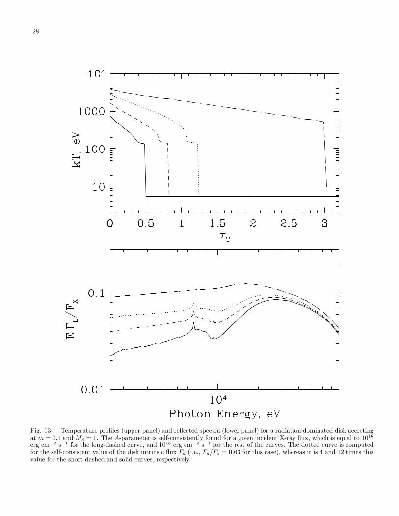
28

Fig. 13.— Temperature profiles (upper panel) and reflected spectra (lower panel) for a radiation dominated disk accretingat m = 0.1 and M8 = 1. The A-parameter is self-consistently found for a given incident X-ray flux, which is equal to 1016

erg cm−2 s−1 for the long-dashed curve, and 1015 erg cm−2 s−1 for the rest of the curves. The dotted curve is computedfor the self-consistent value of the disk intrinsic flux Fd (i.e., Fd/Fx = 0.63 for this case), whereas it is 4 and 12 times thisvalue for the short-dashed and solid curves, respectively.