Transport of Large Scale Poloidal Flux in Black Hole Accretion

Kris Beckwith

Institute of Astronomy

University of Cambridge

Madingley Road

Cambridge CB3 0HA

United Kingdom

krcb@ast.cam.ac.uk

John F. Hawley

Astronomy Department

University of Virginia

P.O. Box 400325

Charlottesville, VA 22904-4325

jh8h@virginia.edu

and

Julian H. Krolik

Department of Physics and Astronomy

Johns Hopkins University

Baltimore, MD 21218

jhk@pha.jhu.edu

ABSTRACT

We report on a global, three-dimensional GRMHD simulation of an accretion

torus embedded in a large scale vertical magnetic field orbiting a Schwarzschild

black hole. This simulation investigates how a large scale vertical field evolves

within a turbulent accretion disk and whether global magnetic field configurations

suitable for launching jets and winds can develop. We find that a “coronal

mechanism” of magnetic flux motion, which operates largely outside the disk

body, dominates global flux evolution. In this mechanism, magnetic stresses

driven by orbital shear create large-scale half-loops of magnetic field that stretch

arX

iv:0

906.

2784

v2 [

astr

o-ph

.HE

] 1

5 O

ct 2

009

– 2 –

radially inward and then reconnect, leading to discontinuous jumps in the location

of magnetic flux. In contrast, little or no flux is brought in directly by accretion

within the disk itself. The coronal mechanism establishes a dipole magnetic field

in the evacuated funnel around the orbital axis with a field intensity regulated

by a combination of the magnetic and gas pressures in the inner disk. These

results prompt a reevaluation of previous descriptions of magnetic flux motion

associated with accretion. Local pictures are undercut by the intrinsically global

character of magnetic flux. Formulations in terms of an “effective viscosity”

competing with an “effective resistivity” are undermined by the nonlinearity of

of the magnetic dynamics and the fact that the same turbulence driving mass

motion (traditionally identified as “viscosity”) can alter magnetic topology.

Subject headings: accretion, accretion discs - relativity - (magnetohydrodynam-

ics) MHD

1. Introduction

Astrophysical jets are seen in such a wide range of astrophysical systems that their cre-

ation must not require particularly unusual conditions. A tentative consensus has emerged

that jets are a natural consequence of accretion, rotation and magnetic fields (for a summary

of this position, see Livio 2000). Although the presence of accretion and rotation are a given

in an accreting system, the presence of magnetic fields has long been considered to be less

certain. However, since magnetohydrodynamic (MHD) turbulence driven by the magnetoro-

tational instability (MRI; see Balbus & Hawley 1991, 1998) accounts for the internal stresses

that drive accretion, one is at least assured that the presence of accretion itself implies the

existence of a tangled magnetic field of some reasonable strength.

But is that enough? Most jet launching mechanisms that have been developed depend on

the existence of a large-scale, organized poloidal field, following in general terms the scenarios

outlined analytically in the influential papers of Blandford & Znajek (1977) and Blandford

& Payne (1982). In the Blandford-Payne model, a large-scale poloidal magnetic field is

anchored in and rotates with the disk. If the fieldlines are angled outward sufficiently with

respect to the disk, there can be a net outward force on the matter. As matter is accelerated

along the rotating fieldlines, its angular momentum increases still further, accelerating and

driving an outflow. In this model the power for the resulting jet comes from the rotation of the

accretion disk. In the Blandford-Znajek model, the jet is powered by the rotating space-time

of a black hole. (In the case of jets from systems with stars rather than black holes, stellar

rotation can play a similar role.) Radial magnetic field lines lie along the hole’s rotation

– 3 –

axis and are anchored in the event horizon. Fieldline rotation is created by frame-dragging

and this drives an out-going Poynting flux. Most simulations that have demonstrated jet-

launching have assumed the existence of a large-scale poloidal (mainly vertical) field in the

initial conditions (see, e.g., the review by Pudritz et al. 2007). Although such simulations

have provided considerable evidence that magnetic fields can be effective in powering jets,

they cannot account for the origin of those fields.

If, as it seems, some sort of large-scale poloidal field is required for jet production, how

can such a field be established in the near hole region? One possibility is an accretion disk

dynamo, presumably working with the turbulent fields generated naturally by the MRI.

A dynamo is an attractive possibility because it has the potential to be ubiquitous. A

number of models have been put forward suggesting how some form of inverse cascade might

occur within the MHD turbulence to generate a large scale field (e.g., Tout & Pringle 1996;

Uzdensky & Goodman 2008), but these scenarios remain speculative and nothing definitive

has been seen in global disk simulations done to date. In any case, the strict conservation

of flux within a volume means that a disk dynamo could produce net flux only through

interactions with boundaries, in this case either the black hole, or by expelling flux to large

radius.

The global advection of net flux is an important process, therefore, whether the disk

functions as a dynamo or net poloidal field is simply carried in to the near hole region from

large radius. Even without any dynamo action, a weak net field might become locally strong

it were concentrated by the accretion process. In the absence of a single field polarity at

large distance, a near-hole net field could nevertheless be built up due to a random walk

process as field is accreted (e.g., Thorne et al. 1986). Whether or not net field can be so

accreted, however, is a matter of some uncertainty. The main concern is that the field would

not be accreted if, as seems intuitively likely, the field intensity declines outward and the

rate of diffusion of the field through the matter exceeds the rate at which matter accretes

(van Ballegooijen 1989; Lubow et al. 1994; Heyvaerts et al. 1996; Ogilvie & Livio 2001).

This competition between inward advection and outward diffusion is typically described in

terms of an effective turbulent accretion viscosity νt determining the accretion rate, and an

effective magnetic diffusivity, ηt that sets the field diffusion rate. The fate of the field is

then determined by the effective magnetic Prandtl number Pm = νt/ηt. In this picture, it is

argued that the relevant scale for effective resistivity is ∼ H whereas the relevant scale for

effective viscosity is ∼ R; consequently, field can be brought inward only if Pm > R/H.

It is far from clear, however, that field transport within MHD turbulence can be de-

scribed in such terms. The picture just described assumes that the fluid motion is inde-

pendent of the field, yet in Nature the dynamical coupling between fluid and field assures

– 4 –

that even weak fields are amplified, and that the effective viscosity νt is, in fact, the result

of magnetic stresses. Thus, there is no kinematic regime in which the Lorentz forces can

be neglected. The resulting MRI-driven turbulence is inherently three-dimensional; indeed,

three-dimensional studies are essential to generating long-term sustained MHD turbulence

due to the fundamental restriction of the anti-dynamo theorem. By contrast, the frame-

work of effective turbulent viscosity and diffusivity is cast in axisymmetry, in the hope that

suitable time- and space-averaging of the field transport process in a fully turbulent, three-

dimensional disk can lead to some value of ηt in much the same way that suitable averaging

of correlations in the magnetic field, normalized to some suitable pressure term (either gas,

magnetic or total pressure) leads to a value of νt. But the primary mechanism by which

magnetic fields change the fluid elements to which they are attached is through magnetic

reconnection driven by the fluid turbulence, not gradual slippage via resistivity. The effec-

tive viscosity and magnetic diffusivity are derived from making the ansatz that stress and

reconnection can be modeled as a viscosity or resistivity, i.e., a constant coefficient multiply-

ing the gradient in orbital rotation rate or magnetic field strength. Whether or not such a

model is appropriate to accretion flows remains to be determined. Finally, net flux and field

topology are global concepts; a purely local description of field motion in terms of transport

coefficients may not be sufficient.

Numerical simulations offer a promising approach to investigate these and other issues

related to global field evolution within accretion flows. Of course, simulations entail their

own set of difficulties: global simulations require adequately fine resolution over a wide range

of radii in the disk body and throughout a good deal of the surrounding coronal region as

well. The numerical grid boundaries should be sufficiently remote so as to minimize artificial

effects on the disk. Although axisymmetric simulations can be of interest, the problem

ultimately must be done in three dimensions because any axisymmetric calculation fails to

describe properly essential properties of both the fluid turbulence and the magnetic field

evolution. Finally, because we need to follow the disk long enough to observe net accretion

in an approximate inflow equilibrium, the duration of the simulation must be long compared

to typical local dynamical times in the disk.

Work along these lines is ongoing. Global, three dimensional black hole accretion sim-

ulations without initial fields threading the disk were carried out and described in a series

of papers beginning with De Villiers et al. (2003). In these simulations initial weak dipole

loops are contained within an isolated gas torus. The subsequent MRI-driven accretion flow

carries the inner half of the initial field loop (with a single sign for the net vertical field

component) down to the black hole, creating radial field as the loop is stretched. Differential

rotation along that radial field leads to rapid growth of the toroidal field, especially within

the plunging region of the flow. This growing toroidal field causes the ejection of a magnetic

– 5 –

tower into the low density funnel region and the establishment of a global dipole field an-

chored in the black hole. This field can then produce a Poynting flux jet if the black hole is

rotating.

Beckwith et al. (2008a) examined several alternative initial field configurations in com-

parison to the dipolar loop. Quadrupolar initial field loops produce a much weaker funnel

field. A similar result was found by McKinney & Gammie (2004) for axisymmetric simula-

tions, and McKinney & Blandford (2009) in a three-dimensional model. A variation proposed

by Hawley & Krolik (2006) and further elaborated upon by Beckwith et al. (2008a) is a series

of dipolar loops contained within the accretion flow. Such loops can lead to the creation of a

temporary net sense of vertical field that can support a significant field in a relativistic outflow

along the rotation axis for a sizable period of time. Beckwith et al. (2008a) also computed

a model that began with a purely toroidal field. In this case the MRI creates turbulence,

field and angular momentum transport, but without creating any overall organization to the

poloidal field. As a consequence, no funnel field is generated.

In this paper we continue our study of the influence of field topology on accretion and

potential jet formation through a three-dimensional general relativistic MHD simulation with

an initial field configuration consisting of a net vertical field passing through an orbiting ring

of gas at modestly large radius. We will investigate the evolution of the disk in the presence

of a net field while determining if such an initial condition can lead to the establishment

of field configurations conducive to jet formation. From this study we hope to gain more

insight into whether or not large scale fields can be advected along with the accreting gas

and to lay the groundwork for further work.

The rest of this paper is structured as follows: In §2, we describe the methodology and

the initial conditions for our simulations. In §3 we discuss their results as they pertain to

magnetic flux motion. Finally, in §4, we summarize our results, compare them with current

models from the literature, and explain their implications for observations of relativistic jets

in Nature.

2. Numerical Details

For this work we employ the general relativistic MHD code GRMHD developed in De

Villiers & Hawley (2003); De Villiers (2006). GRMHD has already been used in several

studies to simulate black hole accretion in three spatial dimensions (De Villiers et al. 2003;

Hirose et al. 2004; De Villiers et al. 2005; Krolik et al. 2005; Hawley & Krolik 2006; Beckwith

et al. 2008a,b). GRMHD solves the equations of ideal non-radiative MHD in the static Kerr

– 6 –

metric of a rotating black hole using Boyer-Lindquist coordinates. Values are expressed

in gravitational units (G = M = c = 1) with line element ds2 = gttdt2 + 2gtφdtdφ +

grrdr2 + gθθdθ

2 + gφφdφ2 and signature (−,+,+,+). The relativistic fluid at each grid zone

is described by its density ρ, specific internal energy ε, 4-velocity Uµ, and isotropic pressure

P . The relativistic enthalpy is h = 1 + ε + P/ρ. The pressure is related to ρ and ε via the

equation of state for an ideal gas, P = ρε(Γ−1). The magnetic field is described by two sets

of variables. The first is the constrained transport (CT; Evans & Hawley 1988) magnetic

field Bi = [ijk]Fjk, where [ijk] is the completely anti-symmetric symbol, and Fjk are the

spatial components of the electromagnetic field strength tensor. From the CT magnetic

field components, we derive the magnetic field four-vector, (4π)1/2bµ = ∗F µνUν , and the

magnetic field scalar, ||b2|| = bµbµ. The electromagnetic component of the stress-energy

tensor is T µν(EM) = 12gµν ||b||2 + UµUν ||b||2 − bµbν .

2.1. Initial and Boundary Conditions

In this study we carry out both axisymmetric and fully three dimensional simulations

around a Schwarzschild black hole. The initial condition, as in previous works (De Villiers

et al. 2003; Hirose et al. 2004; De Villiers et al. 2005; Krolik et al. 2005; Hawley & Krolik

2006; Beckwith et al. 2008a,b), consists of an isolated gas torus upon which a weak magnetic

field is imposed. We use the torus model described by De Villiers et al. (2003) with an

adiabatic index of Γ = 5/3. The initial angular momentum distribution is slightly sub-

Keplerian, with a specific angular momentum at the inner edge of the torus (located at

r = 30M) `in ≡ Uφ/Ut = 6.10. For this choice of `in, the pressure maximum is at r ≈ 40M

and the outer edge of the torus is located at r ≈ 60M . The angular period at the pressure

maximum is Ω−1 ≈ 250M . With this inner edge radius, the resulting accretion flow should

have sufficient radial range to permit a detailed study of the advection of vertical flux. The

choice of angular momentum parameter at the inner edge of the torus, `in, was made so

that the initial torus (and hence the steady state accretion flow) would have a scale height

similar to that of previous simulations (see e.g. Beckwith et al. 2008b). The torus is initially

surrounded by zones filled with zero-velocity gas set to a constant value of density and

pressure. The ratios of these “vacuum” values to the torus maximum are 2 × 10−4 for the

pressure, and 5×10−6 for the density. Because the code is relativistic, the timestep is always

limited by the time for light to cross the smallest cell; high Alfven speeds in the low-density

coronal region do not create any unique difficulty.

The initial magnetic field is homogeneous and vertical, filling the annular cylinder

35M ≤ R ≤ 55M (where R is the cylindrical radius). This configuration differs from

– 7 –

the vertical field used in some previous studies (see e.g. Koide et al. 1999; McKinney &

Gammie 2004; De Villiers 2006) which fills all space, not just through the initial torus. By

isolating the field in this manner, we know that any vertical flux that ends up crossing the

black hole event horizon was brought in from field initially passing through the torus at

large radius, rather than already being present at the horizon in the initial conditions. Also,

because equilibrium field strengths scale strongly with radius, a global vertical field that is

strong enough to be interesting at one radius is likely to be overwhelming at some radii while

negligible at others. We prefer to see the global field strength emerge as an outcome of the

evolution. In our configuration the initial vertical field is subthermal within the torus and is

unstable to the MRI. It should be noted, though, that this initial field configuration is not

in dynamic equilibrium outside of the torus. Also, this is but one very specific realization

of a torus embedded in large scale field. Future experiments will need to explore a wider

variety of initial configurations.

This initial field is computed from the curl of the four-vector potential, i.e.,

Fαβ = ∂αAβ − ∂βAα = Aβ,α − Aα,β. (1)

with only Aφ 6= 0. The vector potential corresponding to a uniform (Newtonian) vertical

field geometry is proportional to the cylindrical radius, i.e.,

Aφ ∝ r sin θ. (2)

The vector potential for the initial field is

Aφ = A0

Rin R < Rin

r sin θ Rin ≤ R ≤ Rout

Rout R > Rout

(3)

where Rin and Rout are 35M and 55M . Outside of those cylindrical radii the field is zero.

A0 was specified so that the ratio of the average thermal to average magnetic pressure inside

the torus is β = 100. At the center of the torus β = 275 and β declines smoothly toward

1 near the edge of the torus. In the surrounding corona, β = 0.038. The initial mass, field

and β distribution is shown in Figure 1.

The simulation we will focus on is three-dimensional with 256×256×64 zones in (r, θ, φ).

The simulation is labeled “VD0m3d.” Given the challenge of adequately resolving such

models and of doing anything like a convergence study, we also carried out two-dimensional

simulations at two different resolutions. In two dimensions we used 256× 256 and 512× 512

zones in (r, θ). The two-dimensional simulations are labeled “VD0m2d” and “VD0h2d”

where the “m” designates medium resolution and the “h” designates the higher resolution

case.

– 8 –

For all models the radial grid extends from an inner boundary at rin = 2.104 to an

outer boundary located at rout = 500M . The radial grid was graded using a logarithmic

distribution that concentrates zones near the inner boundary. An outflow condition is applied

at both the inner and outer radial boundaries. In contrast to the zero net flux simulations

that we have performed previously, magnetic fields pierce the outer boundary in the initial

state. This net flux is kept fixed throughout the simulation, but otherwise the field at the

boundary can evolve. When the fluid velocity normal to the boundary is directed outward we

perform a simple copy of fluid variables into the ghost zones that lie outside of the boundary.

In the case where the fluid velocity is inward, the ghost zones are filled with a cold, low

density, zero momentum fluid at the vacuum value so that only cold, very low density gas

can enter the computational grid. To minimize the influence of the outer boundary it is

located as far away from the region of interest as is feasible. Any torques that arise from

the interaction of the outer boundary with the large scale vertical field should have minimal

influence on the turbulent disk itself.

The θ-grid spans the range 0.01π ≤ θ ≤ 0.99π. This creates a conical cutout that

surrounds the coordinate axis. Such a cutout will prevent flow through the coordinate axis,

but it is computationally advantageous to avoid the coordinate singularity. The size of this

θ-cutout is determined by two considerations. First, light travel times across narrow φ-zones

near the axis sets the timestep, so the cutout should not be too small. In this simulation,

∆t = 2.53×10−3M . The θ cutout must not be too large; initial vertical field should not cross

the θ-cutout before reaching the outer radial boundary at r = 500M . A reflecting boundary

condition is used along the θ-cutout. The θ zones were distributed logarithmically so as to

concentrate zones around the equator.

The φ-grid spans the quarter plane, 0 ≤ φ ≤ π/2. The φ grid is uniform and periodic

boundary conditions are applied. The use of this restricted angular domain significantly

reduces the computational requirements of the simulation. Schnittman et al. (2006) exam-

ined the variance in surface density as a function of φ and found the characteristic size of

perturbations to be around 25. Thus, while some global features may be lost by using a

restricted domain, the character of the local MRI turbulence is captured.

2.2. Magnetic Flux

In analyzing the evolution of the large scale poloidal flux we will make use of the poloidal

flux function, which corresponds to the φ-component of the magnetic vector potential (van

Ballegooijen 1989; Heyvaerts et al. 1996; Reynolds et al. 2006), which we must calculate

from the simulation data. In GRMHD, we directly evolve the components of the Faraday

– 9 –

tensor, Fµν using the alternative form of the induction equation (for further details see De

Villiers & Hawley 2003):

∂δFαβ + ∂αFβδ + ∂βFδα = 0 (4)

The space-space components of Fµν are identified with the constrained-transport (CT) mag-

netic fields via Bi = [ijk]Fjk:

Br = Fφθ; Bθ = Frφ; Bφ = Fθr. (5)

This identification allows us to write the induction equation in the familiar form

∂tBi − ∂j(V iBj − BiV j

)= 0, (6)

where V i = U i/U t. The tensor Fµ,ν is related to the magnetic induction in the fluid frame,

Bα by the relation

Fµ ν = εαβ µ ν Bα Uβ, (7)

where εµ ν δ γ =√−g [µ ν δ γ].

The Faraday tensor can also be written in terms of a vector potential:

Fαβ = ∂αAβ − ∂βAα = Aβ,α − Aα,β. (8)

It is convenient to define an azimuthally-averaged poloidal flux function, Aφ. This can

be derived from the azimuthally-averaged CT field data by noting that the total (spatial)

derivative of Aφ is

dAφ =∂Aφ∂r

dr +∂Aφ∂θ

dθ. (9)

¿From the definition of the Faraday tensor, we have that

Fφθ = Aθ,φ − Aφ,θ; Frφ = Aφ,r − Ar,φ. (10)

After azimuthal averaging, this reduces to

Fφθ = −Aφ,θ; Frφ = Aφ,r. (11)

The space-space components of Fµν are identified with the CT magnetic fields via Bi =

[ijk]Fjk so that

Br = Fφθ = −Aφ,θ; Bθ = Frφ = Aφ,r. (12)

We therefore have that

dAφ = Frφdr − Fφθdθ = Bθdr − Brdθ. (13)

– 10 –

To find the flux from this differential, we could in principle integrate over any poloidal

surface. For the radial motion of vertical flux through the disk, the surface of greatest

significance is the equatorial plane. Because this surface is interrupted by the event horizon,

we must stretch it over half of the event horizon. We will therefore define a flux function

that is the sum of two parts: the radial flux through the inner horizon boundary,

Ψ(θ)|r=rin =

∫ θ

0

dθ′ Br(rin, θ′), (14)

and the vertical flux through the equator,

Φ(r)|θ=π/2 =

∫ r

rin

dr′ Bθ(r′, θ = π/2). (15)

Using these functions, we can determine how the accumulated flux through the top half of

the event horizon depends on polar angle, Ψ(θ), and how much total vertical flux has been

brought to within radius r. The full flux function along the total path is

A(r, θ = π/2) = Ψ(π/2)− Φ(r). (16)

This corresponds to the net flux piercing the surface covering the top hemisphere of the black

hole horizon and the equatorial plane out to radius r. The full vector potential component

Aφ(r, θ) is obtained by integrating the CT variables throughout the computational domain

starting from r = rin and θ = 0. A(r, θ = π/2) is therefore identical to Aφ(r, θ = π/2).

For the three-dimensional simulation, VD0m3d, Br and Bθ are integrated over over the φ-

dimension prior to computing Aφ(r, θ). Given the periodic nature of the φ direction this is

sufficient to compute the total flux piercing the volume bounded by the equatorial plane and

the black hole horizon. We note that this procedure is consistent with the approach adopted

in the calculations of van Ballegooijen (1989), Heyvaerts et al. (1996), and Reynolds et al.

(2006).

3. Global Flux Transport

3.1. Overall evolution

The simulation begins with an isolated torus threaded with a column of vertical field.

The first part of the simulation is marked by relatively rapid evolution of the coronal field

and the surface layers of the torus. Figure 2 shows the evolution of the poloidal magnetic flux

and the density distribution over the time period 1000M ≤ t ≤ 2500M . This process, along

with the subsequent evolution of the flow is also shown in an animation included in the online

– 11 –

edition of this work. We encourage the reader to refer to this material as it clarifies many of

the issues that we shall discuss at length in the remainder of the text. As noted above, the

initial state is not in equilibrium within the corona. There is differential rotation between

the coronal gas and the torus, and the magnetic pressure within the vertical field column

is not balanced by pressure within the initial atmosphere. The field expands radially, and

stresses at the boundary of the disk begin to drive low density gas from the torus outward

along field lines. In the inner half of the torus, low density surface layers move inward in two

thin accretion streams above and below the equatorial plane, dragging poloidal field lines

down to the black hole. This behavior was dubbed an “avalanche flow” when it was observed

in the axisymmetric MHD accretion torus simulations of Matsumoto et al. (1996), and it is a

common feature to accretion models that begin with vertical fields threading the disk (e.g.,

Koide et al. 1999). These surface features develop well before field deeper within the torus

is significantly amplified by the MRI. The surface layers in the outer half of the torus also

evolve, but here mass flows radially outward along the field lines, carrying the field along as

it does so.

By t = 2000M net flux has begun to build up on the black hole horizon, well before any

significant mass accretion has begun. This flux arrives there by a process we call the “coronal

mechanism,” which we discuss briefly here and will discuss again in greater detail in § 3.2.

A typical field line participating in the coronal mechanism may be traced from the outer

boundary at high latitude more or less vertically down to the upper surface of the torus,

where it bends sharply toward the hole near the boundary of the denser region. It goes in

some distance before doubling back (forming a “hairpin” shape) and returning to the torus.

There it passes through the equator, and turns inward to mirror its behavior on the other side

of the equator. A short time later, the apex of each hairpin moves inward and closer to the

equator, where, in the early stages of this simulation when there is little mass at small radii,

it can encounter an oppositely-oriented hairpin from the other hemisphere. Reconnection

ensues, causing the magnetic flux distribution to change essentially instantaneously.

The four panels of Fig. 2 show these structures in differing ways. In the first panel,

an isolated hairpin field line can be clearly seen approaching very close to the horizon. By

the time of the second panel, the bends in this field line have reconnected, attaching it

to the event horizon and liberating a pair of closed loops. Also in the second panel, new

hairpins can be seen forming along the top and bottom surfaces of the disk in the region

20M < r < 30M . These hairpins evolve further and become embroiled in the beginnings of

disk turbulence (the channel modes) in the third and fourth panels.

Magnetic field enters the extremely low-density funnel around the rotation axis by an

offshoot of the coronal mechanism just described. There is initially no field within the

– 12 –

funnel. Once horizontal field lines have been brought close to the black hole, their radial,

near-horizontal components become unstable to the formation of ballooning half-loops that

rise upward into the funnel. These loops are the initial source of field for the funnel. Only

the inner half of the rising loop enters the funnel and, as a result, the field direction changes

sign abruptly at the funnel’s outer edge along the centrifugal barrier.

The coronal process also occurs at radii exterior to the initial pressure maximum of the

torus. There it acts to move net flux progressively outward. Above the disk surface, the

field is stretched out radially, but subsequently bends back down toward the equator, where

reconnection can occur. This transfers the net flux from field lines going through the torus

(those lines now close in large loops) to vertical field lines at large radius.

Thus, in the early phase of the evolution the global topology of the field is rapidly

rearranged through coronal motions without any significant evolution within the main disk.

Although these features result from the initial conditions, the process illustrates how (in

principle) coherent large scale poloidal flux can be rapidly moved over large radial distances.

Although low density surface layers participate in the initial avalanche flow, the dense

part of the torus is largely unaffected by these coronal motions. By t = 2500M , however, the

MRI reaches a nonlinear amplitude throughout the torus and the characteristic structures

associated with the “channel mode” have become visible within the torus. The next stage of

evolution is illustrated in Figure 3 which shows snapshots every 500M in time from 3000 to

4500M . Gas in the torus moves radially both inward and outward in the characteristic chan-

nels as angular momentum is transported along field lines, which are themselves increasingly

stretched into long radial filaments. The channel modes are unstable to nonaxisymmetric

perturbations and rapidly break up, resulting in a turbulent disk without prominent radial

features. In the axisymmetric simulations, these relatively coherent large-scale radial flows

continue to dominate throughout the evolution. This artificial persistence of coherent motion

is a significant limitation of two-dimensional simulations with vertical field.

Accretion into the black hole does not begin until 1650M , and the mass accretion rate at

the inner edge of the disk reaches its long-term mean for the first time shortly after 4500M .

The mass accretion rate then continues to vary by factors of ∼ 2 around this mean through

the remainder of the simulation. The disk achieves an approximate inflow equilibrium within

r ' 25M from time 104M onward. Prior to 104M , the mass in the inner disk (r ≤ 25M) rises

steadily, but after that time, it changes by about 10%, and without any prevailing trend.

The mass accretion rate averaged from 104M until the end of the simulation at 2× 104M is

flat to within 10% for r ≤ 25M . The total mass on the grid at the end of the simulation is

78% of its initial value; of this, 18.8% has gone into the black hole.

– 13 –

The divergence-free nature of the magnetic field means that the total flux is rigorously

conserved except for losses at the boundaries of the computational domain. To measure

the evolution of the total flux we integrate along the black hole horizon from the axis to the

midplane and then out along the equator to the outer boundary. Figure 4 shows this integral

as a function of time. The figure shows that there is no flux lost through the outer radial

boundary during the simulation, but considerable net flux is deposited on the horizon at the

expense of flux through the equator. The majority of the flux brought to the horizon arrives

by t ' 5000M , which implies that the net horizon field is created mostly by coronal motions,

not through disk accretion. During the later stages of more or less steady-state accretion,

the horizon flux grows much more slowly. Relative to its magnitude at t = 5000M , the

horizon flux increases by only 28% over the next 5000M and adds only another 11% during

the last 104M . By contrast, the total mass accreted onto the black hole grows by a factor

of 9 from 5000M to 2 × 104M , with a rate of increase that is approximately constant from

' 104M onward.

The appearance of the overall flow at the end of the simulation is given in Figure 5

which shows the azimuthally-averaged density distribution and the β parameter, and in

Figure 6, which shows the vector potential component Aφ at time t = 2× 104M . There are

several distinct regions. First, there is a low density, strongly magnetized funnel in which the

field lines are primarily radial. Second, there is a corona characterized by large-scale field

lines that loop about creating islands and hairpins, with numerous current sheets separating

closely-spaced regions of oppositely-directed field. Here there are regions of both relatively

strong and relatively weak magnetization; β ranges from ∼ 0.1 to ∼ 10. A thin region of

high β fluid running along the funnel wall marks a current sheet between field lines directed

in opposite radial directions as well as the boundary of the region with strong toroidal field.

Finally, the main disk body remains weakly magnetized, with β ranging from ∼ 10–100.

The disk thickness H/R ranges from 0.1 to 0.15, using the vertical density moment (Noble

et al. 2008) for the definition of H. As can be seen from Figures 3 and 6, substantial parts

of the disk body (most of the disk inside r ' 40M) are actually disconnected from the

large-scale field, their magnetic connections having been broken by the reconnection events

that transferred field both to the horizon and to the outside of the torus. In the outer half

of this region (20M . r . 40M), however, some field lines do pass through the equator and

out through the disk and into the corona.

This initial magnetic field and torus configuration was also simulated in axisymmetry.

While the initial evolutions of the two- and three-dimensional models are similar, once the

MRI sets in within the torus the subsequent evolutions differ dramatically. In axisymmetry,

the channel modes dominate throughout the simulation, creating coherent radial field lines

that extend over large distances. These field structures strongly influence the accretion

– 14 –

of both mass and magnetic flux. Figure 7 compares the flux through the horizon, the

mass accretion rate and the specific angular momentum accreted in simulations VD0m3d

and VD0m2d. The axisymmetric simulation is characterized by very large fluctuations in

mass accretion rate. Similar large fluctuations are seen in the value of the magnetic flux

through the horizon. Note the contrast between the net specific angular momentum jincarried into the hole by the accretion flow in the two- and three-dimensional simulations.

For both plots the dashed line indicates the specific angular momentum of the innermost

stable circular orbit at 6M . The deep minima in the axisymmetric run correspond to strong

torques created by radial field extending through the plunging region. These extended radial

fields are associated with the coherent channel flows seen in axisymmetry, and they have an

obvious strong effect on mass, angular momentum and magnetic fluxes carried into the black

hole. The three-dimensional simulation is qualitatively different. In three dimensions, the

channel modes quickly break up, yielding to genuine turbulence. The accretion rate into

the hole fluctuates, but not nearly as strongly as in axisymmetry. Similarly, only in 3-d can

one speak sensibly about a well-defined net accreted angular momentum per unit rest-mass,

jin. On the basis of these contrasts, we conclude that axisymmetric simulations, while useful

for preliminary investigations of various initial configurations, are of only limited utility in

investigating the long term behavior of MHD turbulent disks.

3.2. The coronal mechanism

The dominant mechanism for bringing flux to the event horizon in simulation VD0m3d is

one that operates primarily in the corona, and not in the disk accretion flow proper. Although

most of the flux is brought in during the first 5000M in time, there is a slow increase in

flux throughout the remainder of the simulation. The majority of this flux appears to be

transported through the continuing operation of the coronal mechanism. The key aspect is

that magnetic field is carried inward by infalling low density fluid. Although this coronal

mechanism operates outside the disk where most of the mass accretion happens, it, too,

depends on angular momentum transport to proceed, and the basic physical mechanism for

angular momentum transport is likewise the same: magnetic torques. Wherever the vertical

field is perturbed so as to create a radial component, orbital shear acting on the radial field

in turn creates toroidal field. Moreover, whenever the orbital frequency decreases outward,

the relative signs of the radial and toroidal fields are always such as to make the r-φ element

of the magnetic stress tensor, brbφ/4π, negative. Such a stress transports angular momentum

outward, tending to accentuate inflow, and therefore growth in the radial field component;

this is, of course, the mechanism of the magneto-rotational instability.

– 15 –

An example of the coronal mechanism in action is given in Figure 8. In this figure,

color contours show the strength of the azimuthally averaged Maxwell stress per unit mass,

overlaid with field lines derived from Aφ(r, θ). For clarity we focus on those field lines

that still pass through the equator in the accretion disk. The first frame, corresponding to

t = 6000M , features a field that runs from the equator vertically upward through the disk

and then down toward the hole before reversing and moving radially outward. The strong

stress per unit mass in the vicinity of the hairpin carries angular momentum away from the

associated matter, enabling it to move inward. In the next frame at t = 6200, the hairpin

moves in radially toward the black hole. The next two frames show a close up view of the

innermost part of the accretion flow at times t = 6440 and 6460M . By the time of the

first one, the inner portion of the hairpin has reached and crossed the horizon. Only 20M

later, the inside hairpin has reconnected, forming a closed field loop. Thus, the net result

of the coronal mechanism at this stage is to attach those fieldlines forming the exterior of

the hairpin to the black hole. These fieldlines then extend out into the corona, ultimately

attaching to the disk at much larger radius.

Although net local inflow of magnetic field is a necessary condition for flux accretion,

it is not a sufficient one; the net flux changes only when reconnection occurs. Local motion

alone is insufficient because magnetic flux is an essentially global concept, so local motion is

not enough to determine net flux transport. This distinction is emphasized by contrasting

the local magnetic inflow rate with global measures. We define the local rate by

VΦ(r, θ) ≡ 1

2π

∫dφV rBθ (17)

averaged over the portion of the simulation during which the trapped flux grows slowly

(5000–2×104M). This is shown in Figure 9, for which the radius was chosen to be 15M . As

this figure shows, the local flux inflow speed is considerably greater just outside the funnel

(|π − θ| ' 0.2π), where it is ' 0.5–1 × 10−4, than in the midplane, where it is nearly two

orders of magnitude smaller.

This local rate of flux inflow is, however, much larger than the global rate of flux accu-

mulation. The global rate is ∂Aφ/∂t, which can be inferred from Figure 4. For the purpose

of this figure, the magnetic flux was separated into the flux piercing the midplane, Φ, and the

flux through the upper hemisphere of the black hole, Ψ. During the early stages of the simu-

lation (before 5000M), ∂Ψ/∂t ' 1× 10−5, but this rate of increase diminishes at later times

by at least an order of magnitude. Thus, the local inflow rate, VΦ(θ ' 0.2π, 0.8π) ' 1×10−4

at r = 15M during the latter 3/4 of the simulation, is as much as two orders of magnitude

greater than the net global rate. In other words, local field inflow alone does not suffice to

create global flux inflow.

– 16 –

Likewise, reconnection on its own is also a necessary condition for flux accretion, but

not a sufficient one. In order for flux accretion to occur, reconnection must result in a

global rearrangement of the field topology. This fact is illustrated by the field structures

displayed in Figure 8. In that figure, a narrow current sheet lies between the two sides of

the hairpin, permitting reconnection to happen there. In order to transfer magnetic flux

inward through the accretion flow and increase the net flux in the funnel, reconnection must

preferentially destroy the side of the magnetic hairpin that lies closest to the midplane. This

is possible because reconnection can also occur across the equator, something that the funnel

field cannot do. Figure 10 illustrates the idea. Coronal hairpin field loops bring field down

to the inner disk, returning along the disk back out to large radius where they eventually

pass through the equator and connect to another hairpin in the opposite hemisphere. The

innermost bend of these hairpins can attach to the horizon. When this happens, the field

appears to be almost a closed loop, with one end of the loop inside the horizon (e.g., the

two inner-disk field lines in the gray region of the diagram). If the two oppositely-directed

portions of one of these loops can meet at intermediate radius, the equatorial flux jumps

inward. This inward jump drastically shortens the time until the entire field loop can accrete

onto the black hole. When that happens, flux of one sign is removed from the horizon above

the equator and flux of the other sign is removed from below the equator, leaving a net

increase in flux piercing each horizon hemisphere.

An example of a reconnection event within VD0m3d that leads to this sort of global

flux rearrangement is shown in Figure 11. In this figure, color contours denote the radial

component of the CT-field, Br, indicating the direction of the fieldline, which are again

overlaid with white contours derived from the azimuthally averaged Aφ(r, θ). Initially (t =

14600M), fieldlines connect large radii to the black hole event horizon through the funnel

region (deep blue region below midplane) and then proceed back out into the disk close to

the midplane (yellow region below midplane). These fieldlines cross the midplane at large

radius and proceed back to the black hole north of the midplane (light blue region north

of midplane), before finally proceeding out to large radius through the funnel region (red

region north of midplane). At time t = 14620M , the oppositely directly fieldlines that lie

just above and below the midplane have reconnected at r ∼ 6M , and the resulting closed

fieldloop (which is still attached to the black hole) is rapidly accreted. This process transfers

flux from the outer disk to r ∼ 6M (where the reconnection event occurs) and then down to

the black hole as the field loop is accreted, arriving at the black hole with the outer edge of

the loop.

The coronal mechanism resembles the flux advection mechanism proposed by Rothstein

& Lovelace (2008) in the sense that most flux transport takes place outside of the disk body,

and that flux in the corona moves inward because magnetic stresses send angular momentum

– 17 –

off to infinity. They emphasize the contrast between the turbulent disk and non-turbulent

flow outside of the disk. We likewise observe that large-scale, relatively laminar flows within

the low-density corona easily move field about; flux-freezing is an excellent approximation

there. On the other hand, there are also several points of contrast between our results and

the model of Rothstein & Lovelace (2008). They argue that in the disk corona, defined as

the region where β ∼ 1, the T zφ component of the magnetic stress tensor could transport

angular momentum outward as effectively as the TRφ component to which attention is more

often directed, allowing the disk surface to move inward. Although this is similar to what

we see in our simulation during the initial avalanche phase, it is different from the dynamics

prevailing at later times. During the accretion phase of the simulation, the coronal field

lines develop MRI-like bends at high altitudes above the disk (>> H), so that the inflow

occurs in the corona rather than along the disk surface. In addition, as shown by Figure 12,

which contrasts the azimuthal averages of −brbφ/ρ and −bθbφ/ρ, there is very little net

angular momentum flux per unit mass in the polar angle direction except in the funnel (at

latitudes not too far from the midplane, bθbφ ' bzbφ). Although the magnitude of T θφ is often

comparable to T rφ , it has very nearly the same probability of having either sign, so that its

mean value is small. On the funnel edge, T θφ is more likely to take angular momentum away

from the disk but has magnitude on average somewhat smaller than T rφ , while in the outer

corona, on average it brings angular momentum toward the midplane.

3.3. Inflow in the disk body

The majority of the net flux on the black hole is brought there by the coronal mechanism

during the initial 5000M of time. However, the flux on the horizon does increase over the last

1.5× 104M and, while the coronal mechanism continues to operate during this interval, it is

possible that part of the flux might be brought in through the accretion disk itself. As the

right panel of Figure 9 makes plain, the local magnetic inflow rate VΦ is roughly two orders of

magnitude smaller in the midplane than it is at the funnel edge. Nonetheless, its magnitude

is still consistent with the total flux inflow rate during the latter part of the simulation. It

may therefore be possible for flux advection directly associated with the accretion flow in

the disk body to account for some part of the flux accumulation during the quasi-steady

accretion phase. In this section we attempt to estimate the size of that contribution.

We begin by comparing the rate of magnetic flux accretion to the rate of mass accretion.

If magnetic flux and mass moved inward in lock-step, the functions

M(r, t) ≡∫ t

0

dt′M(r, t′)/M0 (18)

– 18 –

and

A(r, t) ≡ Aφ(r, t, π/2)/Aφ(rmax, 0, π/2) (19)

would be identical. These quantities are normalized to the initial mass, M0, and the initial

flux; rmax is the outer radius of the initial torus. In Figure 13, we show the time-dependence

of both these quantities at two fiducial radii, just outside the event horizon (left panel) and

at r = 20M (right panel). The former, of course, tells about the flux attached directly to the

black hole and the mass deposited there. The difference between the two plots is the mass

and flux within the accretion disk between the horizon and r = 20M ; here we will refer to

this region as the “inner disk.”

In evaluating Figure 13, one must allow for an important distinction between the his-

tories of mass and magnetic flux: the mass of the black hole must increase monotonically

(and the mass of the inner disk, although not required to do so, generally does), but the

net magnetic flux can increase or decrease, both by magnetic reconnection and by the radial

motion of closed loops. Thus, the inflow of magnetic flux is highly intermittent, and the time-

derivative of flux within some radius can easily be negative. On short timescales, the ratio

of the rate of flux accretion to mass accretion can vary by at least an order of magnitude,

as well as fluctuate in sign. For this reason, a sensible comparison of the rate of magnetic

flux inflow relative to that of mass can be made only in regard to long-term time averages.

In addition, in order to evaluate the efficiency of this process in real disks, we must restrict

these averages to times when the inner disk was in approximate inflow equilibrium: for this

simulation, that means the latter half of the data, from t = 104M to t = 2× 104M . Within

this span, we smooth A(t) by taking a running average 1000M wide and then compose the

ratio of the change in A to M from 104M to 2 × 104M using the smoothed data. We find

that ∆A/∆M ' 0.47 at the horizon, and ' 0.50 at r = 20M . In other words, relative to

the initial amount embedded in the accretion flow, magnetic flux moves inward roughly half

as fast as mass, and these rates are the same at both the horizon and r = 20M . If the mass

is in a state of inflow equilibrium, the equality of these two ratios shows that the magnetic

flux in the inner disk is also in equilibrium.

This ratio of inflow rates may be contrasted with the local ratio of magnetic flux to

mass. Looking beyond the short-timescale fluctuations in the plots of A(t) in Figure 13,

one sees that the average values of the flux at the horizon and the flux contained within

r = 20M are very similar. In other words, the vertical magnetic flux through the inner

disk, Φ(r = 20M), contributes very little to A. Time-averaging over the last 104M of data,

we find that it is only ' 0.86% of the initial flux, and it appears that what flux there is is

confined to the outer part of the inner disk. By contrast, averaged over the same period, 5%

of the initial mass can be found in the inner disk. Thus, in the inner disk, the time-averaged

flux/mass ratio is only 17% of the initial value.

– 19 –

To reconcile this flux/mass ratio with the accreted flux/mass ratio, there are only two

possibilities: either the magnetic flux moves in at the same rate (or slower) than the mass

and (at least) 2/3 of the flux reaching the horizon between 104M and 2 × 104M arrived

there via a different route (most likely the coronal mechanism), or the magnetic flux on

average moved inward three times faster than the mass. We view the former alternative as

much more plausible. Note, however, any flux delivery from outside the inner disk must be

balanced by flux losses from the inner disk to the horizon because the magnetic inflow rate

at r = 20M is nearly the same as at the horizon.

Next we further explore the nature of the magnetic flux equilibrium in the inner disk,

using two different views of this quantity. Figure 14 shows the distribution of the vertical flux

function Φ(r) time-averaged over the last 5000M of the simulation and normalized to the

initial flux value. For comparison, we also plot in that figure both the initial flux distribution

and the final mass distribution in the disk, both likewise normalized to the initial total. The

radial derivative dΦ/dr shows the magnitude and sign of the vertical magnetic field piercing

the equator. We see that, like the mass, vertical flux has spread away from its initial location,

both in and out, but, as already mentioned, a much smaller part of the net magnetic flux

than the mass resides in the inner disk.

The time-dependence of the magnetic flux in the inner disk over the last 104M in time is

illustrated in Figure 15. As this figure shows, not only is the magnetic flux contained within

the inner disk a rather small part of the total, it fluctuates in time, frequently going negative.

Little sign of any long-term trend can be seen, consistent with our contention that the inner

disk magnetic flux has reached a statistical equilibrium. The frequent sign changes of the

local net flux suggest that the poloidal magnetic field lines in the inner disk predominantly

close within the inner disk.

Moreover, the magnetic field corresponding to the net flux is a very small fraction of the

total field within the disk. Figure 16 shows the azimuthally averaged value of Bθ through

the equator at the end time as a function of radius, along with the initial value. The MRI

has generated considerable field of both signs throughout the disk. Local regions of the disk

have a net vertical flux, but their contrasting signs lead to little contribution to the total

disk flux. The global net flux is present only as a slight positive excess moving both inward

and outward with time.

To reach the state described by these figures, most of the large-scale magnetic connec-

tions to the disk matter must have been reconnected away. But this should come as no

surprise because we have already seen that a significant part of the original flux has moved

by reconnection from the disk to the horizon. The matter in the inner disk has little net

flux because it has been largely bypassed through the coronal mechanism. Thus, while the

– 20 –

MRI has created a large effective turbulent viscosity in the sense that considerable mass has

accreted from the location of the initial torus, very little net flux has moved with it. In

other words, within the disk, turbulence created by the MRI transports angular momentum

rapidly and drives accretion, but very little flux moves with the accreting mass.

3.4. Strength of the Funnel Field

Lastly, we raise the question of whether in the very long-term the magnetic flux on the

horizon would continue to grow. If it is regulated by a combination of the magnetic and gas

pressure near r = 6M , and these are in an approximately time-steady state, one might expect

that further flux accumulation on the horizon would have to stop. Figure 17 supports this

idea. This figure shows that the magnetic pressure inside the funnel, the magnetic pressure

in the inner accretion flow, and the gas pressure in the inner accretion flow are well correlated

with one another in a temporal sense, even while all three change by more than two orders

of magnitude over the course of the simulation. The time-dependent data show fluctuations

that are so large, however, that the much slower accumulation of flux seen in Figure 13 is

well below the noise, so our data on magnetic and gas pressures cannot answer any questions

about long-term saturation of magnetic flux attached to the horizon.

That the magnetic and gas pressures should be closely related is an old idea (Rees

et al. 1982; MacDonald & Thorne 1982), but there is also a long history of controversy

about whether the magnetic field pressure in the funnel should be closer in magnitude to the

(poloidal) magnetic pressure or the gas pressure in the inner disk. For example, Ghosh &

Abramowicz (1997) and Livio et al. (1999) argued that as the poloidal magnetic field strength

in the disk is subthermal, the funnel field strength should be regulated by it rather than the

gas pressure. In the simulation presented here, the total, i.e. poloidal plus toroidal magnetic

pressure in the disk is smaller than the gas pressure for the duration of the simulation (i.e.

the field remains subthermal), and the magnetic pressure from the field in the funnel lies

between these two candidate regulators, sometimes closer to one and sometimes closer to the

other. Thus, the funnel field is consistently stronger than the poloidal field in the disk.

The relevance of the inner disk poloidal field to the strength of the funnel field seems

to be rather limited based upon what we observe about the process carrying flux to the

horizon. The field in the funnel is nearly radial, and its total intensity is determined by the

poloidal flux that is delivered to the black hole over the course of the simulation. This flux

delivery system is the coronal mechanism, and so it should not be surprising that the poloidal

flux within the accretion disk itself plays at most a secondary role (e.g., by determining the

rate of reconnection and accretion of flux loops). Instead, simple pressure-matching in the

– 21 –

inner regions of the accretion flow—be it gas, (total, mostly toroidal) magnetic or radiation

pressure—appears to be important in regulating how much flux may be attached to the black

hole. We speculate that when the flux on the horizon has a total field intensity larger than

would be consistent with the gas and magnetic pressure in the nearby accretion flow, the

rate of reconnection along the funnel field boundary rises, so that the field approaching the

black hole is entirely in closed loops and does not add to the net flux on the horizon.

4. Summary, Discussion & Conclusions

In this paper we investigate the evolution of an accretion torus embedded in a large-scale

vertical magnetic field orbiting a Schwarzschild black hole, with a view toward studying how

magnetic flux moves relative to the accretion flow. The simulation stretched over 2.0×104M

in time, corresponding to 80Ω−1 at the initial torus pressure maximum, long enough to

establish inflow equilibrium in the inner disk for the second half of the simulation. Of

particular interest is how the net vertical field evolves, and whether or not a field distribution

consistent with the formation of jets or winds can develop. We trace the evolution of the net

poloidal flux distribution with a particular focus on net flux that becomes attached to the

black hole. Our primary result is that a significant fraction of the initial flux—' 27%—is

brought to the black hole horizon, even though only a rather smaller fraction of the initial

mass—' 19% is accreted. The flux attached to the horizon supports a coherent poloidal

field within the evacuated axial funnel, a requirement for the creation of a Blandford-Znajek

type jet (if the black hole rotates, which it did not in this simulation). The mass and flux

are carried inward through distinct mechanisms: the mass by turbulent stresses within the

accretion disk, and the flux by large-scale motions in the low density corona.

Most of the global magnetic flux motion is mediated by a novel mechanism that we

have dubbed the coronal mechanism. Rather than the gradual “diffusive” process that had

been the focus of most previous discussions of magnetic flux motion in accretion flows,

in this mechanism the flux is brought directly down to the horizon as the net flux jumps

discontinuously when large-scale magnetic loops reconnect across the equator. The same

orbital shear that creates angular momentum transport in the disk body by correlating radial

and azimuthal magnetic field also acts in the corona; the difference is that in the corona the

resulting stress leads to the formation of large-scale loops stretched rapidly inward rather

than to MRI-driven turbulence. These stretched loops can reconnect to oppositely-directed

field at much smaller radius than their footpoint, leading to sudden macroscopic radial

changes in the location of magnetic flux. Although the coronal mechanism acts particularly

rapidly during the initial transient phase of the simulation, it continues to dominate flux

– 22 –

motion throughout the simulation, including the long period during which the inner disk is

in approximate inflow equilibrium. We might therefore reasonably expect it to be a property

of actual accretion disks.

The same reconnection that creates global relocation of net flux simultaneously creates

closed field loops within the disk body. For this reason, the flux/mass ratio within the

accretion flow is suppressed by a factor of order unity relative to what it is in the initial

state. Earlier global disk simulations have, in most cases, assumed zero net flux for reasons

of simplicity and computational convenience; the coronal mechanism might, in fact, make

this assumption a reasonable approximation to the magnetic field in typical disks. The

suppression of flux/mass in the disk body also makes conventional advection of flux in

direction association with mass accretion relatively inefficient.

As seen in previous simulations (particularly Beckwith et al. 2008a), if the overall field

topology at the black hole is dipolar, the funnel field can be relatively immune to reconnection

and hence long-lived. We conjecture that the funnel field amplitude is determined by pressure

balance with the gas and (total, mostly toroidal) magnetic pressures in the inner disk and

coronal regions. Future experiments could test this hypothesis by running much longer

simulations with more available net field to see if the field strength levels off or continues to

build.

As with any simulation, our results are subject to some uncertainty due to the lim-

itations inherent in a numerical solution. One concern is the importance of reconnection

to the overall flux evolution. In our numerical simulation, reconnection occurs at the grid

scale when oppositely signed field components are brought together. Although leaving the

microscopic rate of such an important process to numerical effects is a concern, the overall

motions that lead to the formation of current sheets and subsequent reconnection area driven

by events on much larger scales. In this sense, we might argue that the rate of reconnection

seen in the simulation is relatively independent of our gridscale. We have not, however,

demonstrated that our results are numerically converged, although the global field motions

in the axisymmetric simulations carried out at two different resolutions were very similar.

Furthermore, the thermodynamics of these simulations are incomplete because energy lost

to numerical magnetic reconnection and numerical cancellation of fluid velocities is not cap-

tured; conversely, we do not account for radiation in any way, either as a cooling agent or

as a contributor to the pressure. One thing that is clear, regardless of any other numerical

limitation, is that axisymmetric simulations are of limited utility. In addition to the con-

straints associated with the anti-dynamo theorem, the vertical field channel modes remain

dominant throughout the simulation, giving a qualitatively distinct evolution at late time.

Three dimensional simulations are essential for studying long term, steady-state behavior.

– 23 –

To place our somewhat surprising results in context, it is worthwhile contrasting them

with previous suggestions about how magnetic flux moves through accretion flows. These

are quite disparate, for they have in general been based on approximate analytic arguments.

We examine three principal approaches, of which one has received much more attention than

the others.

The greatest amount of attention has been given to a picture in which the matter moves

inward by an unspecified angular momentum transport process (called “viscosity”, but not

thought to be literally that) while the magnetic field diffuses relative to the matter through

another mechanism called “turbulent resistivity”, but similarly unattached to specific mi-

crophysics (e.g., van Ballegooijen 1989; Lubow et al. 1994; Heyvaerts et al. 1996; Ogilvie &

Livio 2001). The ratio between this effective viscosity and resistivity (the nominal Prandtl

number), would then determine whether the flux mostly moves inward with the mass, or

instead diffuses outward relative to the mass fast enough to avoid much net inward motion.

This approach rests upon two little-examined assumptions: First, that the overall flow

can be regarded as if it were laminar and time-steady, and second, that the behavior of

the underlying turbulence can be reduced to parameters (an advection rate and a diffusion,

i.e., resistivity, coefficient) whose values are independent of the magnetic field. With these

assumptions, field motion in the disk body governs field motion far away from the disk,

and one may describe the field evolution in the language of linear diffusion. Unfortunately,

neither assumption applies to real accretion flows.

It is now well-established that angular momentum transport in accretion disks is due to

turbulent magnetic stresses driven by the MRI. Consequently, the magnetic field structure

is neither laminar nor time-steady. Even in the corona, where the MRI per se does not

occur, the same basic physics leads (as we have earlier discussed) to irregular field motions.

There is therefore no direct connection between local field motion deep inside the disk (e.g.,

resistive diffusion) and the position of the corresponding field lines far away. Moreover, as

we have emphasized, flux is a global concept, not a local one; the coronal mechanism, for

example, could never be described by a local theory of this sort.

The second assumption, that the evolution of the field can be described in terms of

simple resistive and viscous diffusion operating on a background field gradient is similarly

problematic. Accretion is driven by nonlinear magnetic stresses; because the effective inflow

velocity arises only from an average of a strongly fluctuating velocity field, it is non-local in

both time and space. Similarly, the breakdown in ideal MHD happens primarily by driven

reconnection, the rate of which depends on the structure and magnitude of both the magnetic

and velocity fields. As a result, neither the mean rate at which magnetic field is carried from

place to place nor any tendency for its structure to smooth is either independent of or linear

– 24 –

in the field strength.

In fact, the formulation in terms of a competition between “viscous” and “resistive”

diffusion breaks down in an even more fundamental way. Where there is net flux passing

through the disk body, the very same MHD turbulence that transports angular momentum

simultaneously decouples the flux from the matter through turbulence-driven reconnection.

Field lines associated with flux passing through the equator develop bends that readily break

off as closed loops. The matter moves inward with the closed loops while the flux stays in

place. Thus, in dramatic contrast to the conventional prediction, rapid “viscous” accretion

can, and apparently does, co-exist with largely stationary flux, while the “resistivity” that

permits this decoupling has no particular impact on smoothing the field distribution.

Moreover, there is relatively little net flux passing through the disk because reconnection

associated with the coronal mechanism detaches it efficiently. In other words, most of the

flux motion occurs in an “end-run” that bypasses the disk altogether, so that it has rather

little to do with any activity in the disk body, “viscous”, “resistive”, or other.

Local smoothing of field structures can occur, but it is questionable whether one can de-

fine an overall diffusion coefficient to describe its rate. For example, Guan & Gammie (2009)

have recently attempted to quantify magnetic diffusion in the context of MRI-driven MHD

turbulence using shearing box simulations. They imposed a sinusoidally varying vertical

field with an amplitude above the background due to the MRI-turbulent flow and observed

the subsequent decrease in this mode’s Fourier power. The peak vertical field amplitudes

studied vary from 10–80% of the initial toroidal field strength. They found that the decay

time for the imposed feature is several tens of Ω−1, with the decay rate an increasing func-

tion of the perturbation amplitude. These results indicate that local field gradients can be

smoothed within the turbulent flow, but it is unclear to what degree the inferred average

diffusion coefficient depends on the specific situation studied. In particular, in accretion

disks, the net field, the part determining the flux, is, especially in the disk body, small in

magnitude compared to the fluctuating turbulent field. When the dynamics are strongly

nonlinear, spreading of structures in this small net field may proceed in a way very different

from spreading of larger amplitude structures; in fact, the motion of the net field may have

much more to do with the dynamics of the fluctuating field than to its own disposition.

For all these reasons, therefore, we see no useful way to describe the results of the present

simulation in the traditional language of arbitrarily specified transport coefficients applied

to gradients of the time-averaged magnetic field.

Two other concepts have recently been studied. One of these (Rothstein & Lovelace

2008; Lovelace et al. 2009) in some respects is a blend of the “advection/diffusion” picture

– 25 –

and the coronal mechanism. On the one hand, it uses the conventional formalism of fixed

transport coefficients; on the other hand, it relies heavily on field line motions in the corona.

These two approaches are united by supposing that the MRI and its resulting turbulence

are suppressed in the corona, so that it suffers neither “turbulent viscosity” nor “turbulent

resistivity”. Consequently, coronal motion is dominated by vertical transport of angular

momentum, in a magneto-centrifugal wind when the effective Prandtl number is large, and

in a Poynting flux-dominated outflow otherwise. The result is that (for most parameters),

the upper surface of the disk moves inward, carrying the footpoints of the large-scale flux

with it, while the flow in the midplane is outward.

As we have previously discussed, the fundamental physical element of the MRI, the

creation of substantial magnetic stresses by orbital shear, does operate within the corona, and

strongly—this is the foundation of the coronal mechanism. Despite these coronal motions,

this is not a significant source of angular momentum transport for the main accretion disk.

Although the instantaneous amplitude of the magnetic T θφ stress is typically sizable, outside

the funnel its sign fluctuates so that we see no significant net vertical transport of angular

momentum from the disk. In addition, the net fluid radial velocity in the midplane, although

small compared to its rms value, is inward. Nonetheless, our results are consistent with their

suggestion that magnetic stresses carrying angular momentum outward through the corona

can be effective in moving field lines inward. Because the mass density in the corona is so low,

removing a comparatively small amount of angular momentum can lead to large-scale field

motions. Because the subsequent motions are not dominated by turbulence, flux freezing

remains effective within the coronal plasma.

In the second of the two recent suggestions for how flux moves in accretion flows, Spruit

& Uzdensky (2005) propose that the flux motion is not controlled by a simple gradient,

but rather by the dynamics of intermittent field bundles. These authors suggest that mag-

netized patches could accrete relatively rapidly from angular momentum losses through a

wind. Further, if such fields were strong enough to suppress the MRI, then turbulence,

and subsequently magnetic reconnection, would be greatly reduced for those patches. While

such magnetized patches would not themselves lead to a significant net magnetic flux pass-

ing through the disk per se, they could accumulate at the central black hole until the field

strength itself suppressed further accretion. Such a scenario is similar to that of the mag-

netically arrested accretion model of Narayan et al. (2003). Strong nonaxisymmetric field

structures appear in a simulation of Igumenshchev (2008) where a strong field is contin-

ually injected at the outer boundary, providing some support for the Spruit & Uzdensky

(2005) concept. In our simulation, we do see nonaxisymmetric variations in the vertical

flux throughout the disk, but not in the form of local pockets of intense vertical flux, nor

do we see either any significant disk wind or any interruption of the accretion flow due to

– 26 –

“magnetic arrest.” Nonetheless, we agree with Spruit & Uzdensky (2005) in emphasizing

the intermittency of the flow and the potential importance of nonaxisymmetries.

The study carried out here is, of course, only a first step, and the results presented here

point to several avenues of investigation with future numerical experiments. For example,

simulations that continue for longer times and begin with net field at larger radii can better

explore the efficacy of the coronal mechanism. In particular longer simulations with more

available net field are required to see if the field strength in the funnel levels off or continues

to build over time. Simulations in the Kerr metric with non-zero spin parameters could

also study directly how magnetic flux evolution and the coronal mechanism relate to jet

launching and collimation. The requirements of three spatial dimensions and increased

spatial resolution will continue to make these investigations challenging.

This work was supported by NSF grant PHY-0205155 and NASA grant NNX09AD14G

(JFH), and by NSF grant AST-0507455 (JHK). We thank Sean Matt, Jim Pringle, Chris

Reynolds, Charles Gammie and Scott Noble for useful discussions. We acknowledge Jean-

Pierre De Villiers for improvements to the algorithms used in the GRMHD code. The

simulations described were carried out on the Teragrid Ranger system at TACC, supported

by the National Science Foundation.

REFERENCES

Balbus, S. A., & Hawley, J. F. 1991, ApJ, 376, 214

——. 1998, Reviews of Modern Physics, 70, 1

Beckwith, K., Hawley, J. F., & Krolik, J. H. 2008a, ApJ, 678, 1180, arXiv:0709.3833

——. 2008b, MNRAS, 390, 21, 0801.2974

Blandford, R. D., & Payne, D. G. 1982, MNRAS, 199, 883

Blandford, R. D., & Znajek, R. L. 1977, MNRAS, 179, 433

De Villiers, J., & Hawley, J. F. 2003, ApJ, 589, 458

De Villiers, J., Hawley, J. F., & Krolik, J. H. 2003, ApJ, 599, 1238

De Villiers, J., Hawley, J. F., Krolik, J. H., & Hirose, S. 2005, ApJ, 620, 878

De Villiers, J.-P. 2006, ArXiv Astrophysics e-prints, astro-ph, astro-ph/0605744

– 27 –

Evans, C. R., & Hawley, J. F. 1988, ApJ, 332, 659

Ghosh, P., & Abramowicz, M. A. 1997, MNRAS, 292, 887

Guan, X., & Gammie, C. F. 2009, ArXiv e-prints, 0903.3757

Hawley, J. F., & Krolik, J. H. 2006, ApJ, 641, 103, astro-ph/0512227

Heyvaerts, J., Priest, E. R., & Bardou, A. 1996, ApJ, 473, 403

Hirose, S., Krolik, J. H., De Villiers, J., & Hawley, J. F. 2004, ApJ, 606, 1083

Igumenshchev, I. V. 2008, ApJ, 677, 317, arXiv:0711.4391

Koide, S., Shibata, K., & Kudoh, T. 1999, ApJ, 522, 727

Krolik, J. H., Hawley, J. F., & Hirose, S. 2005, ApJ, 622, 1008

Livio, M. 2000, in American Institute of Physics Conference Series, Vol. 522, American

Institute of Physics Conference Series, ed. S. S. Holt & W. W. Zhang, 275–297

Livio, M., Ogilvie, G. I., & Pringle, J. E. 1999, ApJ, 512, 100, arXiv:astro-ph/9809093

Lovelace, R. V. E., Rothstein, D. M., & Bisnovatyi-Kogan, G. S. 2009, ArXiv e-prints,

0906.0345

Lubow, S. H., Papaloizou, J. C. B., & Pringle, J. E. 1994, MNRAS, 267, 235

MacDonald, D., & Thorne, K. S. 1982, MNRAS, 198, 345

Matsumoto, R., Uchida, Y., Hirose, S., Shibata, K., Hayashi, M. R., Ferrari, A., Bodo, G.,

& Norman, C. 1996, ApJ, 461, 115

McKinney, J. C., & Blandford, R. D. 2009, MNRAS, 394, L126, 0812.1060

McKinney, J. C., & Gammie, C. F. 2004, ApJ, 611, 977, astro-ph/0404512

Narayan, R., Igumenshchev, I. V., & Abramowicz, M. A. 2003, PASJ, 55, L69, arXiv:astro-

ph/0305029

Noble, S. C., Krolik, J. H., & Hawley, J. F. 2008, ArXiv e-prints, 0808.3140

Ogilvie, G. I., & Livio, M. 2001, ApJ, 553, 158, arXiv:astro-ph/0007474

Pudritz, R. E., Ouyed, R., Fendt, C., & Brandenburg, A. 2007, in Protostars and Planets

V, ed. B. Reipurth, D. Jewitt, & K. Keil, 277–294

– 28 –

Rees, M. J., Phinney, E. S., Begelman, M. C., & Blandford, R. D. 1982, Nature, 295, 17

Reynolds, C. S., Garofalo, D., & Begelman, M. C. 2006, ApJ, 651, 1023, arXiv:astro-

ph/0607381

Rothstein, D. M., & Lovelace, R. V. E. 2008, ApJ, 677, 1221, arXiv:0801.2158

Schnittman, J. D., Krolik, J. H., & Hawley, J. F. 2006, ApJ, 651, 1031, arXiv:astro-

ph/0606615

Spruit, H. C., & Uzdensky, D. A. 2005, ApJ, 629, 960, arXiv:astro-ph/0504429

Thorne, K. S., Price, R. H., & MacDonald, D. A. 1986, Black holes: The membrane paradigm

(Black Holes: The Membrane Paradigm)

Tout, C. A., & Pringle, J. E. 1996, MNRAS, 281, 219

Uzdensky, D. A., & Goodman, J. 2008, ApJ, 682, 608, 0803.0337

van Ballegooijen, A. A. 1989, in Astrophysics and Space Science Library, Vol. 156, Accretion

Disks and Magnetic Fields in Astrophysics, ed. G. Belvedere, 99–106

This preprint was prepared with the AAS LATEX macros v5.2.

– 29 –

Fig. 1.— Initial torus and field configuration. White contours denote magnetic field lines,

color contours density distribution (left panel) and the gas β parameter (right panel).

– 30 –

log10 ρ

−10.000 −8.717 −7.434 −6.151 −4.867 −3.584 −2.301

Fig. 2.— Initial evolution of the flow in simulation VD0m3d showing the advection of the

vertical field from the initial location of the torus to the black hole. White contours are

magnetic field lines, color contours show the density distribution. From left to right, the

panels correspond to times t = 1000, 1500, 2000, 2500M . The color scale is the same as in

Figure 1. By t = 2500M , the funnel region has become strongly magnetic pressure dominated

and two large scale channel modes have formed within the initial torus.

– 31 –

log10 ρ

−10.000 −8.717 −7.434 −6.151 −4.867 −3.584 −2.301

Fig. 3.— Growth and subsequent break up of the vertical field MRI channel mode in sim-

ulation VD0m3d. White contours are magnetic field lines, color contours show the density

distribution. From left to right, the panels correspond to times t = 3000, 3500, 4000, 4500M .

The color scale is the same as in Figure 1. By t = 4500M , the disk has become turbulent;

large scale MRI modes persist within the corona.

– 32 –

Fig. 4.— Total flux Aφ integrated from the axis along the horizon to the equator and then

out along the equator to the outer boundary. The equatorial component, Φ, and the horizon

component, Ψ are shown separately. The vertical scale is in units of the total initial flux.

The total flux is unchanged through the evolution; losses in the equatorial flux are accounted

for in net flux through the horizon.

– 33 –

Fig. 5.— Azimuthally-averaged gas density (left panel) and plasma β (right panel) at time

2× 104M in simulation VD0m3d.

– 34 –

Fig. 6.— Contours of Aφ(r, θ), displayed both in color and as poloidal field lines (isosurfaces

of Aφ(r, θ)) at time 2× 104M in simulation VD0m3d.

– 35 –

Fig. 7.— Comparison between results from the two-dimensional (VD0m2d) and three-

dimensional (VD0m3d) simulation. Top panel shows the flux through the horizon, Ψ for

VD0m2d (solid line) and VD0m3d (dashed line). The middle panel shows the net mass ac-

cretion rate through the horizon in units of the initial torus mass. The bottom panel shows

the specific angular momentum carried into the hole as a function of time for simulations

VD0m2d and VD0m3d. The strong coherent radial fields in the two-dimensional system

create large fluctations in these quantities.

– 36 –

log10 (−br bφ/ρ)

−4.000 −3.333 −2.667 −2.000 −1.333 −0.667 0.000

Fig. 8.— Evolution of a magnetic “hairpin” in the corona during the turbulent steady state.

Color contours show the azimuthal average of stress per unit mass, −brbφ/ρ, and are overlaid

with the poloidal field structure (white lines), which are kept fixed between the panels. From

left to right, the top panels show times t = 6000, and 6200M (top row). The bottom row

shows the near-hole region at times t = 6440 and 6460M . During this time a reconnection

event takes place within the field hairpin.

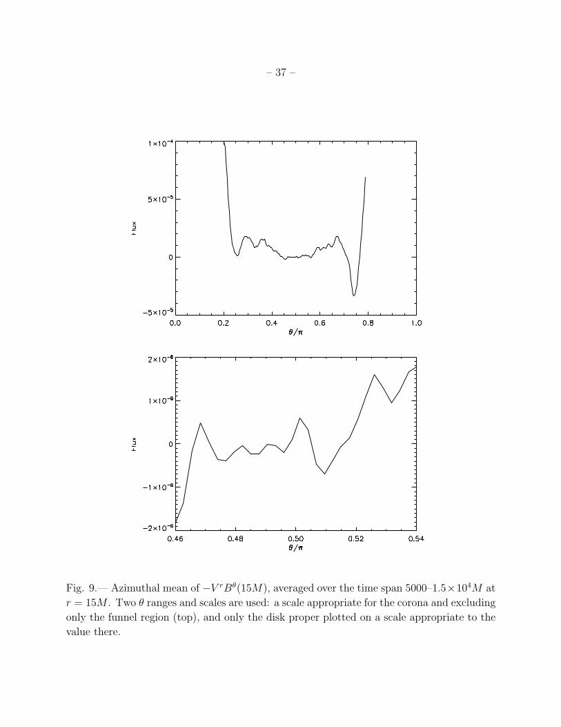
– 37 –

Fig. 9.— Azimuthal mean of −V rBθ(15M), averaged over the time span 5000–1.5×104M at

r = 15M . Two θ ranges and scales are used: a scale appropriate for the corona and excluding

only the funnel region (top), and only the disk proper plotted on a scale appropriate to the

value there.

– 38 –

Fig. 10.— Schematic of the field line structure in the coronal mechanism. Field lines within

the coronal are carried in toward the black hole, forming a hairpin-like structure. When the

hairpin connects to the horizon flux is added to the funnel field and opposite-signed flux is

added to the disk (shaded region). Reconnection across the equator (dashed line) allows this

field to form loops that accrete. Accretion of those field loops results in an increase of the

net horizon flux.

– 39 –

Hr

−0.100 −0.067 −0.033 0.000 0.033 0.067 0.100

Fig. 11.— Reconnection event that occurs in the disk and leads to the rapid transport of

poloidal magnetic flux from the outer disk to the black hole. Color contours show Br and

are overlaid with the poloidal field structure (white lines), which are kept fixed between the

panels. From left to right the panels show t = 14600, 14620, and 14640M .

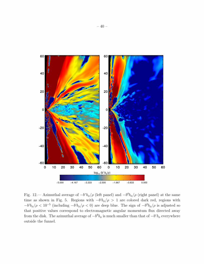
– 40 –

log10 (bi bφ/ρ)

−5.000 −4.167 −3.333 −2.500 −1.667 −0.833 0.000

Fig. 12.— Azimuthal average of −brbφ/ρ (left panel) and −bθbφ/ρ (right panel) at the same

time as shown in Fig. 5. Regions with −bibφ/ρ > 1 are colored dark red, regions with

−bibφ/ρ < 10−5 (including −bibφ/ρ < 0) are deep blue. The sign of −bθbφ/ρ is adjusted so

that positive values correspond to electromagnetic angular momentum flux directed away

from the disk. The azimuthal average of −bθbφ is much smaller than that of −brbφ everywhere

outside the funnel.

– 41 –

Fig. 13.— Fractional accretion of magnetic flux A (solid curve) and massM (dashed curve)

as functions of time. Because we stored shell-integrated mass accretion rates every 1M in

time, but the full 3-d data required to compute the vector potential only every 10M , the

latter curve has greater time resolution than the former. (Top) At r = 2.1M . (Bottom) At

r = 20M .

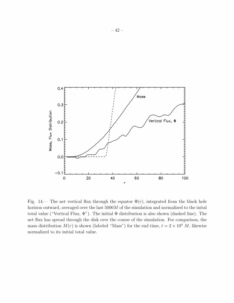
– 42 –

Fig. 14.— The net vertical flux through the equator Φ(r), integrated from the black hole

horizon outward, averaged over the last 5000M of the simulation and normalized to the inital

total value (“Vertical Flux, Φ”). The initial Φ distribution is also shown (dashed line). The

net flux has spread through the disk over the course of the simulation. For comparison, the

mass distribution M(r) is shown (labeled “Mass”) for the end time, t = 2× 104 M , likewise

normalized to its initial total value.

– 43 –

Fig. 15.— Space-time contours of the net vertical flux through the equator Φ(r), integrated

from the black hole horizon outward for the inner disk during the second half of the sim-

ulation, normalized to the total initial flux. Never very large in magnitude, the integrated

magnetic flux in this region fluctuates in sign.

– 44 –

Fig. 16.— Azimuthal average of the absolute value of |Bθ| (solid line) and the average of

Bθ (dot-dashed line) along the equatorial plane at t = 2 × 104 M (solid line) along with

the initial Bθ distribution (dashed line). The vertical field remains relatively strong but

experiences fluctuations in sign throughout the disk body. The net flux is a small positive

bias in the vertical field value.

– 45 –

Fig. 17.— Azimuthally-averaged magnetic pressure as a function of time at two locations:

inside the funnel near its base (r = 6M , θ = 0.044π; solid curve); and in the inner accretion

flow (r = 6M , θ = π/2; dotted curve), and azimuthally-averaged gas pressure in the inner

accretion flow (also r = 6M , θ = π/2; dashed curve).