Stars and Galaxies

Tom TheunsOffice 307

Institute for Computational CosmologyOgden Centre for Fundamental Physics

Durham Universityand

University of AntwerpCampus Drie Eiken

tom.theuns@durham.ac.uk

2006-2007

Prologue

Before the beginning

This course on galaxies runs over 14 lectures. The aim is to give you anoverview of galaxy properties and of some of the physical processes that wethink shape galaxies. In contrast to the beauty of stellar physics, you’ll seethat galactic physics is often much more murky and complex – a bit likeweather predictions: we (think we) know the physics, but even so it still isdifficult to make accurate calculations. And often, we don’t know the physicsvery well – or even at all. On the bright side, galaxies are beautiful. And wecan in principle probe physics on scales which are impossible to reach withinthe laboratory and so learn about really fundamental physics – just recallthe recent excitement about the possible non-zero value for the cosmologicalconstant. Anyway, I hope you’ll enjoy the lectures.

As to the organisation of the course, I will basically follow the structure ofSimon Morris, i.e. there will be hand-outs after each lecture, but more up-to-date versions will appear on the web in DUO. Look there as well for (mostof) the pictures that I show during the lectures. Suggestions on materialincluded in this course, its presentation, and lists of errors in the notes, willbe most appreciated.

And for those that are only interested in passing their exams: there willbe two questions on galaxies. The first consist of 5 very short questions whereyou’re asked to describe very briefly some concepts that we have discussed.For example, what is the interstellar medium, and how do we observe it.Given five differences between football and basketball. The second type ofquestion usually starts from a derivation that we’ve done. The end of thequestion is something you have not seen, but is very similar to what we havedone.

1

My source of knowledge

Although this field is continually evolving, much of the basics is of coursetext-book stuff. The web provides a very valuable source of information,not just for pictures. Often, satellite mission web-pages have extremely welldesigned pages. Some links you might want to look at (and where I got manyof the pictures) are:

• http://www.seds.org/

• http://www.aao.gov.au/images.html/

• http://hubblesite.org/newscenter/archive/

• http://teacherlink.ed.usu.edu/tlnasa/pictures/picture.html

• http://astro.estec.esa.nl

• http://space.gsfc.nasa.gov/astro/cobe/cobe home.html

• http://astro.estec.esa.nl/Hipparcos/

• http://astro.estec.esa.nl/GAIA/

and the books I’ve used are

1 Carroll & Ostlie, Modern Astrophysics, Addison-Wesley, 1996

2 Zeilik & Gregory, Astronomy & Astrophysics, Saunders College Pub-lishing, 1998

3 Binney & Merrifield, Galactic Astronomy, Princeton, 1998

4 Binney & Tremaine, Galactic Dynamics, Princeton, 1987

(I’ll refer to these as CO, ZG, BM, and BT.) The first two are quite moregeneral, [3] provides a nice overview on galaxies in much more detail than I’lldo, and [4] of course concentrates on the dynamics of galaxies. [1] containseverything you need to know, in [2] you can often find the basics formulatedin a very clear way, and [3] and [4] are where you could start looking if youwant to know more.

2

A truly excellent web site where much of what I’ll discuss is explainedreally well with many pictures, and by someone who knows what he’s talkingabout, is by Chris Mihos, who is at the department of astronomy, CaseWestern University. You’ll find it at:http://burro.astr.cwru.edu/Academics/Astr222/index.html, and you’ll recog-nise some of the picture in my course as originating from there.

3

Chapter 1

Introduction

1.1 Historical perspective

Galaxies were discovered in the 20th century. This is surprising, since youcan see many of them on a clear night with the naked eye. They differ fromstars in that they are extended. For example, the nearby Andromeda galaxyhas an extent of several degrees (diameter of full moon is 0.5 degrees). Andthe Large and Small Magellanic clouds in the Southern hemisphere, are evenbigger. And the nearest galaxy (which was only discovered in the last years!)extends over a significant fraction of the whole sky! The reason that theydon’t stand-out very clearly is not because they are faint, it is because theyare so large. Since they are large, their light is distributed over a wide area,and our eyes do not pick-out the small increase in surface brightness over thenight sky.

They were called nebulae to distinguish them from stars. However, thereare other extra-solar objects which are also extended on the sky: PlanetaryNebulae, star clusters, super nova (SN for short, and SNe for the plural)remnants, for example. Since before the 1920s we didn’t know the distanceto those objects, it wasn’t clear what were the relations between them. Andso many of the catalogues of nebulae, for example Messier’s catalogue (objectsdenoted by an ‘M’ , like M31, which is Andromeda), or NGC (New GeneralCatalogue, Dreyer 1888), contain a baffling variety of unrelated objects.

Immanual Kant, the German philosopher, suggested that the reason wesee a faint band of stars across the night sky – usually called the Milky Way(MW for short) – is because most MW stars, as well as the Sun, lie in a

4

disk. And so, when you look out at night in the plane of the disk, yousee a faint band of light. Galileo already had resolved this band of lightinto stars. Kant claimed that most of the other nebulae were just othergalaxies. It took until the 1920s before this hypothesis was proved correct.The historical introduction in BM is well worth reading.

As a final point: why study galaxies? Are they in some sense the mostimportant building blocks in the Universe? I like BMs reasoning: stars areapparently huddled together in galaxies. And since (not surprisingly if youthink about it) humans can see stars, we are naturally inclined to studythem. But, for example, although a cluster of galaxies contains thousands ofgalaxies, they are by no means its main constituent. Most of the mass is indark matter – which we cannot see at all. But most of the baryons are in hotgas, which we can observe with X-ray satellites, but we cannot see. And sothe choice to study galaxies is a bit human centred: our eyes can see them.

1.2 Bringing order to the zoo of galaxies

Before we start doing any calculations, it might be a good idea to look aroundus and make an inventory of what types of galaxies are out there. There aremany good web pages to start, for example I like http://www.taas.org/gnto/astropic.html,because it shows pictures made with a small telescope – so those are galaxiesas you might have seen them yourself, if you are an amateur astronomer.http://www.aao.gov.au/images.html/ shows professional images. Such pro-fessional pages (for example the Hubble Space Telescope (HST) archive) tendto contain a large fraction of unusual galaxies – simply because those are theones that astronomers tend to study.

1.2.1 Vocabulary

Colours. These images are taken through broad-band filters, typically1 V,Band R, and so each individual exposure might as well be in black and white,the relative blackness being a measure of how much, or how little, of the lightin that wavelength band fell on that part of the photograph/CCD. Imagestaken trough different filters are then combined to produce a colour image,scaling the different bands trying to mimic the colour your eye would see.

1The names give an indication of the corresponding wavelength region, B for blue, Vfor visual, R for red, U for UV (in the direction of the UV-that is), I for IR.

5

Sometimes though, one of the filters used is a narrow-band filter, for ex-ample Hα or O[III]. These filters block all light which is not in a narrowrange around the hydrogen Hα transition, or a transition in doubly ionisedoxygen. Combining such a narrow-band image with images made with oth-ers filters produces a false colour image, i.e. the colour of the object is nothow your eye would see it, but the colour coding has been chosen to bringout a particular feature – for example Hα emission. The really pretty colourpictures of Planetary Nebulae are false colour images.

Luminosity, flux and surface brightnessA star emits a certain amount of energy per unit time. For example

the Sun has a luminosity L = 1L = 3.4 × 1026W. This quantity is notobservable however: what we can measure is how much of this energy wereceive, per unit time, per unit surface area (assuming you put the surfaceperpendicular to the radiation!), at a given distance from the source. Theobservable quantity, energy received per unit time per unit of surface area, iscalled flux. Clearly the flux will depend both on the luminosity of the star,and on its distance. How?

Consider a sphere of radius r, with the star at the centre. Since the starwill distribute all of its energy equally over the surface of the sphere, the fluxF = L/(4πr2). (As an exercise, find the unit of flux).

It is the flux of the star that determines how bright it appears to be. In-deed, star A may be brighter than star B, either because it is more luminous,LA LB, or because it is nearer to us, rA rB.

Although F is in principle observable, in practise astronomers expressbrightness in terms of magnitudes m, where the apparent magnitude m =−2.5 log10(F )+C, where C is some constant that depends on the magnitudesystem used. Since the F depends on distance, so doesm, it is not an intrinsicquantity of the star – hence ‘apparent magnitude’. The absolute magnitude,M , is the apparent magnitude when r = 10pc.

Since a galaxy contains many stars, we can also talk about its luminosity,and the flux we receive from it. However, because galaxies are spatiallyextended2, we can also try to measure what fraction of the flux comes fromthe centre of the galaxy and what fraction comes from the outer parts, say.This gives rise to the term surface brightness.

Consider a small patch of galaxy, namely that part contained in a (small)

2Very nearby stars can be resolved with special techniques.

6

solid angle dΩ. Observationally we can measure the flux, dF , of light, com-ing from the part of the galaxy contained within dΩ. The quantity dF/dΩ iscalled surface brightness (SB), and so it has dimensions energy/time/area/steradian.3

The surface brightness of a galaxy does not depend on its distance. To seethis, assume that the patch of galaxy contained within dΩ contains N stars,with mean luminosity L, when it is at a distance r. The surface brightnessSB=N L/(4πr2)/dΩ. Now increase the distance to the galaxy by a factorof 2. The flux from each individual star will decrease by a factor 22, sinceF ∝ 1/r2. However the number N of stars within dΩ will increase by afactor 22, since the physical size of the patch enclosed by dΩ will doublewhen r doubles. Hence SB is distance independent4, therefore whereas withbrightness there was an intrinsic quantity (luminosity), and an observableone (flux), there is only one surface brightness.

A galaxy’s SB depends on its distribution of stars. Assume a face-ongalaxy at distance r has a surface density Σ of stars (in stars/pc2, say),all with the same luminosity L. The surface area of galaxy dS, containedwithin a solid angle dΩ, is dS = dΩ r2. Therefore the number, dN , of starswithin dΩ is dN = Σ dS = Σ dΩ r2. The flux received from a single staris L/(4πr2, and therefore the flux received from all N stars within dΩ isdF = (L/(4πr2)) × (Σ dΩ r2) = ΣLdΩ/(4π). The surface brightness is theflux per unit solid angle, is df/dΩ = ΣL/(4π) is distance independent, as wesaw before.

1.2.2 Galaxy properties

Looking at the different images of galaxies, it becomes immediately clear thatthere are two basic types, elliptical and spiral galaxies.

Ellipticals (also called early type galaxies, E galaxies for short)

• have smooth light distributions, where the isophotes (lines of constantSB) have (nearly) elliptical shapes. They are denoted as En, wheren = 10(1− b/a), and a and b are the semi-major and semi-minor axisof the ellipse. So, an E0 is round, and an E7 is flattened, n = 7 is abouthow flattened E’s get. A 3D ellipsoidal shape, with semi-axes a, b and

3A solid angle is usually expressed in steradians, or arc sec2, seehttp://whatis.techtarget.com/definition/0,,sid9 gci528813,00.html.

4This is only true for relatively nearby galaxies. On cosmological distance the SBdecreases with distance because of the redshift.

7

c (ordered as a ≥ b ≥ c), is called oblate when a = b > c (a pancake),prolate when a > b = c (a cigar), and tri-axial when a > b > c (asquashed American football). E’s are probably tri-axial.

• have no current star formation

• have old stars

• have little gas and dust

• occur preferentially in groups and clusters of many Es

• have little evidence for rotation, so the stars must have large randommotions to keep the system from collapsing (also called a hot stellarsystem)

Spirals (or late type galaxies, S galaxies for short)

• have most of the light coming from a thin disk. Seen face on, it isnearly circular, seen edge on, it is nearly a line. In their centre, theyoften have a nearly elliptical stellar system, similar in shape to a smallelliptical, called a bulge. In addition, some have a bar as well.

• have light profiles with a characteristic spiral pattern

• have star formation going on, especially in their spiral arms

• have both old and young stars

• have gas and dust

• seem to avoid dense groups, and are very rare in clusters

• have large rotational velocities, enough to keep their stars on circularorbits.

We inferred the stellar properties from the fact that E galaxies tend tobe redder than S. This suggested that they lack the young massive starsthat produces most of the blue light. Hence our inference that the stellarpopulation is likely to be older, with the massive stars that have short lifetimes already dead. We will see later that the SB distribution, SB(r), arequite different for these two types.

8

These are the archetypal properties of such systems, of course there areexceptions. For example, some ellipticals do have dust, as well as evidence forrecent star formation. Some even have a small disk. Given that some spiralshave a very large bulge, and some ellipticals have a disk, the distinctionbetween the two types is not always as clear as you might think. Clearly itwould be interesting to know what processes are responsible for forming anelliptical vs a spiral in the first place.

Both types are seen to have hundreds and sometimes thousands of globularclusters (GCs for short). These are very dense, spherical, gravitationallybound systems of typically 105 to 106 low mass stars, and they are usuallyfound in a spherical distribution around their parent galaxy. The Milky Wayhas about 150 of them.

There are many schemes for classifying galaxies. A good scheme shouldbe unambiguous, and ideally have some physics behind it. Classificationalong the Hubble sequence (Fig. 1.1) is still very popular. It divides galaxiesin ellipticals and spirals. Spirals are divided in two strands, according towhether they are barred (SB), or not (S). The sequence has the shape ofa tuning fork – the Hubble tuning fork. Along the handle of the tuningfork, the range goes from E0 to E7. The sequence then forks, toward thetop are unbarred spirals (S), along the bottom are barred spirals (SB). Bothstrands are further divided along the sequence (away from the handle), as Satoward Sc, and analogously SBa to SBc, depending on the relative strengthof bulge to disk, and, correlated with this, how tightly/loosely wound thearms are. Sa’s and SBa’s have a large bulge and tightly wound arms, Sc’sand SBc’s have a much smaller bulge, and more loosely wound arms. Finally,any galaxy that does not fit into the sequence, is called irregular (Irr).

The physical scale of galaxies is huge: E’s can have masses from as little as107M to as much as 1013M, with linear sizes ranging from a few tenths ofa kpc to hundreds of kpc. In contrast, spirals tend to be more homogeneous,with masses 109–1012M, and disk diameters from 5 to 100kpc or so.

Hubble thought (incorrectly) that this sequence was due to evolution,where galaxies evolve from being E0s, toward Sa or Sba, and later evolvingin the more loosely wound Sc’s or SBc’s. Therefore these types are also calledearly type and late type. So E’s are also called early type, and Ss are calledlate type. And an Sc is a late-type spiral, and Sa an early type spiral. Weknow now that this is not the way galaxies evolve, yet these names are stillwidely used.

There are other reasons why this is not a particularly good scheme. For

9

Figure 1.1: The Hubble sequence.

10

example, galaxies may look quite different depending on the filter you use toobserve them in.

Another type you’ll often come across are cD galaxies, which stands forcentral Dominant: these are very large ellipticals, found in the centres ofclusters, with a faint but very large outer halo of stars.

Yet another type are called S0 (or SB0 when barred) or lenticulars: theyare the divide in Hubble’s sequence between E and S. They have disks withoutgas or dust, and no recent star formation.

Galaxies can fail to fit in the sequence, for example because they recentlyhad a tidal encounter with another galaxy. This typically leads to spectaculartidal arms, like the case of e.g. the Antennae.

Most smaller galaxies are of the Irregular type: no disk, no nice sphericaldistribution of stars either, but a loose aggregate of stars, like for example theMagellanic Clouds. Since there are far more small than large galaxies, mostgalaxies are in fact of type Irr. The aim of these lectures is to understandwhich types of observation can be used to describe these different types abit better (the ‘biology bit of the lectures’), and also try to understand thephysical processes behind them. May be you’ll be surprised to learn that, formany of the most basic questions you might think of, such as – why are somegalaxies of type E, and others of type S?, or, why do Ss have spiral arms?– we are only just beginning to understand the underlying physics, and wehave by no means a well defined, generally accepted textbook answer. Maybe something for you to work on, when you start doing astronomy researchyourself?

11

1.3 Summary

After having studied this lecture, you should be able to

• Describe the main galaxy types, Es and Ss, and list five characteristicsof each

• Describe some properties of Globular Clusters.

• Define surface brightness, and show it to be independent of distance.

• Derive the relation between the surface density of stars in a galaxy, andits surface brightness.

• Know where to find web-pages with images of galaxies.

12

Chapter 2

The discovery of the MilkyWay and of other galaxies

Around the 1920s a great debate was raging about the nature of the nebulaeand the size of the Milky Way. There were two camps. According to onecamp, the nebulae were structures within the Milky Way, probably proto-planetary systems or something similar, and the Sun was near the centreof MW. The other camp claimed that many of the nebulae were galaxiesoutside of the MW, and the Sun was at large distance from the centre of theMW. The reason they couldn’t decide was mainly because they didn’t knowhow to determine distances to the nebulae. The reason the first group gotit wrong was quite interesting. And so we’ll go through this debate, hopingwe can learn from the mistakes. Before we do this, let’s describe the mainobservables, and observing techniques.

2.1 The main observables

Star clusters There are two types of star clusters, i.e. groups of 103s to105s of stars. Globular Clusters (GCs) are spherical, gravitationally boundsystems of 105 − 106 old stars. Most galaxies contain 10s to 1000s of GCs,spherically distributed around the parent galaxy. The MW has about 150GCs. Stars form in the MW disk out of large molecular clouds. Sometimes,after the gas has been dispersed, the newly formed stars are gravitationallybound to each other, in what is called an Open Cluster. These typicallycontain of order 104 stars. So they differ from GC in that they are typically

13

smaller, have young stars, and lie in the galactic plane. Star clusters areof great importance for studies of stellar evolution, since we know all thestars in such a cluster have (more or less) the same age, distance and initialcomposition, and hence they provide us with a sample of stars in which theonly (or at least the main) difference is the stellar mass.

Star counts Star counts can be used to probe the number density of starsas a function of position. In the early days, William Herschel and his sistercounted the numbers of stars as function of their magnitude in many (700!!)directions in the sky, by spending (most?) nights gazing through his tele-scope! Later, photographic plates were used for the same purpose. From thefact that the number of stars falls with magnitude much faster perpendicularto the disk, than in the plane of the disk, one deduced that the stars aroundthe Sun are indeed distributed in a disk, with axes ratio about 5:1.

How does it work? Suppose you count the number of stars dN , in a givensolid angle dΩ, that have flux fainter than F , but brighter than F −dF (withdF > 0). If all stars have luminosity L, then stars with flux F are at distancer, given by F = L/(4πr2). Similarly, stars of flux F − dF are at distancer + dr, given by F − dF = L/(4π (r + dr)2). If dr r, then dF = 2F dr/r.The volume of the fraction of a spherical shell that falls within a solid angledΩ, between r and r + dr is dV = dΩ r2 dr. Combining all this we get forthe number of stars per unit solid angle, with flux between F and F − dF

dN

dΩ= n(r) r2 dr = n(r) r2 r

2FdF =

1

2(L

4πF)3/2 n(r)

dF

F. (2.1)

The function dN(F )/dΩ in the plane of the MW drops much slower withdecreasing F than perpendicular to the plane, meaning n(r) drops muchslower within the disk, then perpendicular to it. Which is because the starsare distributed in a disk around the Sun, not spherically symmetric. This ishow you can determine n(r) by counting stars.

Standard candles are objects with a known absolute property, for exam-ple a known size, or known luminosity. It is then possible to determine thedistance to the standard candle by measuring their angular size , or appar-ent luminosity, respectively. A most important example is that of Cepheidvariables. Henrietta Leavitt studied variable stars in the Magellanic Cloudin 1912. She found a relation between the period P of the variation ∆m andthe magnitude m of these Cepheids. Since all these stars are at (nearly) the

14

same distance, this must mean it is actually a relation between the absolutemagnitude M and P . There are many types of variable stars, but Cepheidshave many advantages as standard candles (a) the shape of their light curve(i.e. luminosity as function of time) is a very characteristic sawtooth pattern,(b) they are luminous - and so can be seen out to large distances and (c)the P (M) relation has little scatter. Unfortunately, they are also relativelyrare. RR Lyrae are similar to Cepheids, but occur in a different type ofstar. They are also used as standard candles. Of course, to get an absolutedistance, we need somehow to find the distance to some Cepheids or RRLyrae using another method, for example using the parallax.

Parallax Stretch your arm, point your index finger upward, and look withyour left eye alone toward a distant wall. Now, look with your right eye alone:your finger seems to have moved with respect to the background. You’ve done(your first?) parallax measurement. If the wall is sufficiently distant thenthere is a relation between how much your finger appears to move (in degrees,say), the length of your arm, and the distance between your eyes. If you nowone distance (e.g. between your eyes), you can determine the other (lengthof arm).

You can increase the distance between your eyes to twice the distanceearth-Sun, by looking at the same object half a year apart. Since one canrelatively easily measure angles to a fraction of an arcsec 1, we have a newdistance unit: the pc. An object at 1pc distance has a parallax of 2arcsec.Let’s compute how much this really is. Consider an equi-lateral triangle, withtwo sides of length 1pc third side 1AU. By definition 1pc/1AU=1arcsecinradians2 Hence

1pc =180× 3600

πAU ≈ 206265AU . (2.2)

Unfortunately, this literally doesn’t get use very far: the distance to eventhe nearest stars is of this order. We’ll come back to the distance scale later.

The parallax and Cepheid variables are the first two steps in the distanceladder, which use one method (e.g. parallax) to calibrate another distancemeasure (e.g. Cepheids), that then can be used to calibrate another distanceindicator, and so go to go to greater and greater distances. The Hubble spacetelescope recently measured Cepheids in the Virgo cluster (at a distance of

1An arcsec is a 60th of an arc minute, or 1/3600th of a degree. Now we can do muchbetter!

2We’ve used the fact that this angle is very small.

15

∼ 17Mpc), thereby providing the first accurate distance to that cluster ofgalaxies, and getting an accurate measurement of Hubble’s constant in theprocess.

2.2 The main players, their measurements,

and their mistakes

The famous Dutch astronomer, Jacobus Kapteyn and his collaborators, starteda major project of counting stars around the 1900s, to determine once andfor all the structure of the MW. He counted stars on photographic plates asfunction of apparent magnitude (brightness), in several directions.

His analysis basically confirmed Herschel’s picture: the MW is a flattenedelliptical system, with stellar density n decreasing away from the centre. ndrops to half its central value at 150pc perpendicular to the MW plane, and800pc in the galactic plane. The Sun is at 650pc from the centre. This is infact wrong but for an interesting reason.

Kapteyn assumed that the flux received drops as 1/r2. One reason thiscould be wrong is because of absorption or scattering of the stellar light,in which case the flux will drop faster than 1/r2. Of course, not takingabsorption into account would give you the wrong answer, and Kapteyn wasfully aware of this. How can we test whether absorption is important? ForRayleigh scattering off atoms, there is a colour dependence: blue light isscattered more than red light. As a consequence fainter and hence moredistant stars would be expected to be redder on average. Now Kapteynfound this indeed to be the case, yet the amount of reddening was too smallfor absorption to be important. The mistake in the reasoning was that theabsorption is due to dust, not Rayleigh scattering. Dust absorption is muchless colour dependent, and so the small reddening measured by Kapteynactually implied a much greater dimming of the distant stars. Consequentlythe size of the MW as well as the position of the Sun in it came out wrong.

The American astronomer Harlow Shapley estimated the distances to thebrightest globular clusters using their RR Lyrae variables, and found theywere not centred around the Sun, but around a point 15kpc away in thedirection of Sagittarius. This was in conflict with the Kapteyn universe – itseemed difficult to reconcile the Sun to be near the centre of the MW, yetthe centre of the globular cluster system not to coincide with the centre of

16

MW? There was no clear way how to reconcile these different data, and sothe issue remained unresolved for some time.

Meanwhile, another famous Dutch astronomer, van Maanen, found thatsome of the nebulae had proper motions, implying they were nearby, withinthe MW. (He compared the positions of the nebulae on plates taken severalyears apart). It was generally accepted these nebulae were probably proto-planetary systems, or something like that. van Maanen himself, but alsoEdwin Hubble later redid the proper motion measurements with better data(using a better telescope), and both failed to reproduce the proper motions.van Maanen probably just made a mistake! In the 1930s, Hubble made hiseven more famous discovery that the spectral lines of atoms in other galaxiesare shifted to the red, by an amount proportional to the distance to thegalaxy.

So it was a combination of mistakes (van Maanen), and not taking intoaccount the importance of dust (Kapteyn), that led to the confusion. Inthe end, Hubble’s better data clinched the matter. He resolved Cepheidsin Andromeda, one of the bigger nebulae, and found a distance of 300kpcand so clearly outside of the MW. In one great swoop, the universe becausemuch bigger, and in addition it was found to be expanding! It is difficult tounderestimate the significance of this discovery.

The 1920s were of course a period of great economic depression. Butfrom the scientific point of view, they must have been tremendously exciting.In only a couple of years, the general theory of relativity was formulated,quantum mechanics revolutionised physics, the MW was recognised to bejust one of millions of other galaxies, the Universe was found to be big andexpanding

It was not until the 1930s that Trumpler found what had been wrongwith Kapteyn’s results. He studied Open Clusters in the MW plane. Heassumed them to be all of about the same size, and so got an independentrelative distance for them. He used another estimate of their distance, basedon ‘spectroscopic parallaxes’ . This involves predicting the luminosity of astar from its spectrum. He showed that the more distant clusters (as judgedfrom their angular size), appeared to have unusually faint stars in them. Orequivalently, that the more distant clusters (as judged from their photometricparallax) were larger. Clearly, something was wrong here. He correctlyinterpreted this, as due to the fact that the light from these more distant starswas strongly attenuated. By comparing the reddening with the attenuation,it was clear that a given amount of reddening corresponded to much more

17

dimming than you’d expect for Rayleigh scattering. And hence Kapteyn’sscales were wrong.

Before I summarise this in a time-line, just think of the fact that Einsteinformulated his theory of general relativity, on which the current cosmologicalmodels are still based, before this puzzle was resolved. In fact, our view ofthe Universe around Einstein’s time, was just plain wrong. I guess he rightlypaid little attention to what the astronomers of his days told him!

2.2.1 Time-line

1610 Galileo resolves the MW into stars

1750 Immanual Kant suggests that some of the other Nebulae are othergalaxies, similar to the MW.

end of 1700s Messier and Herschel catalogue hundreds of Nebulae. Herschel countsstars, and deduces that the Sun lies near the centre of an ellipticaldistribution with axes ratio 5:5:1

1900-1920 Kapteyn counts stars, decides wrongly that extinction is unimportant,and deduces the MW to be 5kpc × 5kpc × 1kpc big, with the Sun at650pc from the centre.

1912 Leavitt discovers the P (L) relation for Cepheids.

1914 Slipher measures large (1000s km s−1) velocities for some Nebulae, andfinds evidence for rotation. The spectra he takes suggests presenceof stars, not of gas. A clear indication these are not proto-planetarystructures in the MW, but other galaxies.

1915 Shapley finds the centre of the MW’s globular cluster system to be faraway from Kapteyn’s MW centre.

1920 van Maanen claims (erroneously) that some spiral nebulae have a largeproper motion, suggesting they are within the MW.

1920 Shapley and Curtis debate publicly over the size of the MW, but thematter is not settled.

18

1923 Hubble resolves M31 (Andromeda) into stars, using the newly com-missioned 100-inch telescope. Given the large inferred distance meansthat M31 must be outside the MW. He also discovers Cepheids, andthe distance to M31 is estimated at 300kpc. So Andromeda us indeedanother galaxy.

1926 Lindblad computes that Kapteyn’s MW is so small, it cannot gravita-tionally bind its Globular Clusters. But Shapley’s much bigger MWcould.

1927 Jan Oort shows that several aspects of the local motion of stars cannicely be explained if the Sun (and the other nearby stars), is on anearly circular motion around a position 12kpc away in the directionof Sagittarius. Nearly the same position as found by Shapley, andimplying a much larger MW than Kapteyn’s.

1927 larger MW picture, where many of the nebulae are extra-galactic MWs,gains general acceptance.

1929 Hubble discovers his expansion law. His derived value is a factor of 10too large!

1930 Trumpler uses open clusters to show the importance of extinction, andexplains why Kapteyn’s measurement were faulty

1930-35 Hubble’s new data confirm the modern picture of galaxies, and demon-strates van Maanen’s measurements must have been wrong.

And so in a very short time indeed, three sweeping changes in our viewof the visible universe took place:

• an 8-fold increase in the size of the MW

• the acceptance that many of the nebulae were external galaxies

• the universe is expanding

19

2.3 Absorption, scattering and reddening

What is the effect of dust on the light we detect from distant stars? Supposethe wavelength of the light is much smaller than the size of the dust grains(bricks, say) – then you could compute the dimming just from the geometriccross-section of the bricks along the line of sight. Consider a ray of light withintensity I. The amount of light of this ray absorbed per unit distance, willsatisfy

dI

dr= −AI , (2.3)

which expresses the fact that each distance dr will absorb a constant fractiondI/I = −Adr of the light. This is what we want since, if the light sourcewere twice as bright, then the bricks will stop twice as many photons. Ais some constant, which will depend on the size of the bricks, and theirnumber density. This equation is easy to integrate, and the solution is I =I0 exp(−Ar). Taking the log of both sides, we find that the effect on themagnitude will be ∆m = Ar. So the relation between apparent (m) andabsolute magnitude (M) will change from m−M = 5 log(r)− 5 to

m−M = 5 log(r)− 5 + Ar , (2.4)

due to the effect of absorption. So the unit of A is magnitudes per kpc .(Careful readers will notice that I have slightly changed the definition of Aalong the way, but you get the idea.)

If the size of the particles is of order of the wavelength λ of the light, thenit is not a good approximation to use the geometric cross-section of the dustgrains to estimate absorption. The amount of absorption (the value of A)will then depend on λ, and so AV 6= AB, say: absorption in the B band willdiffer from that in the V band, and so absorption will also lead to a colourchange (reddening, since the longer wavelengths get less absorbed than theshorter ones).

Applying Eq.(2.4) to two bands, we find

(m−M)B = 5 log(r)− 5 + AB r

(m−M)V = 5 log(r)− 5 + AV r

EB−V ≡ (mB −mV)− (MB −MV) = (AB − AV) r . (2.5)

The quantity EB−V is called the colour excess, note that it is the differencebetween the observed and intrinsic colour of the star,

EB−V = (B−V)observed − (B−V)intrinsic . (2.6)

20

Trumpler’s measurements, and also laboratory measurements, show thatfor interstellar dust grains

EB−V ≈ 1

3AV r . (2.7)

This is a crucial result. Reddening and hence EB−V, is easy to measure,

and so if we do this for stars of known distance, we find3 AV ≈ 1mag kpc−1.If we now measure EB−V for another star of known colour (from stellarevolutionary models say) we can estimate r.

3The amount of dust is not the same everywhere: there are regions where the absorptionis much stronger, not surprisingly called dark clouds, and some directions along which theabsorption is much less, a well known direction is called Baade’s window.

21

2.4 Summary

After having studied this lecture, you should be able to

• Describe the Great Debate, give the points in favour of each camp, anddiscuss the problems with their arguments.

• Derive the relation between the stellar density and star counts

• Explain what a standard candle is.

• Explain why Cepheids and RR Lyrae variables are good standard can-dles.

• Explain what parallax is, and know how the distance to nearby starscan be measured using their parallax.

• Explain how parallax and Cepheids can be used to walk-up the distanceladder.

• Explain how Hubble’s observations revolutionised our view of the MWand the realm of the Nebulae.

• Derive the effect of scattering by dust on the apparent magnitude andcolour of distant stars. Know the approximate value of the interstellarabsorption in the MW.

22

Chapter 3

The modern view of the MilkyWay

Our observational picture of the MW has been clarified due to steady hardwork and occasionally in great leaps with the advent of new technologies.

3.1 New technologies

3.1.1 Radio-astronomy

Radio astronomy used the new technology developed for radar and opened anew window for astronomers to gaze through. Roto-vibrational1 transitionsin molecules have low excitation levels, which are ideally suited to probe thelow temperatures in interstellar clouds. Because the wavelengths of thesetransitions are long, one can build very large dishes to observe them, andalso it is more straightforward to build interferometers.2

1Most transitions you know, which occur in the visible and UV-part of the spectrum,are electronic transitions: in emission, they occur because an electron changes from ahigher energy state to a lower one, e.g. from n = 2 → 1 for the hydrogen Lyman-αtransition, and from n = 3 → 2 for the hydrogen Hα transition. And in absorption, theygo the other way around. But molecules also have excited levels due to their rotation orvibration. Since these are also quantum-mechanical the energy levels are quantised. Andtransitions between them correspond to rotational or vibrational transitions. Since theenergy-levels are lower they correspond to longer wavelengths – typically mm and cm: inthe radio.

2One way to think of this is to realise in good ‘mirror’ the departure from the idealshape should not be larger than some small fraction of the wavelength of the radiation

23

An electron moving in a magnetic field will feel an acceleration, causingit to circle around the field lines. Such synchrotron radiation can also beobserved in the radio.

Today, one regularly combines data from radio-observatories across theearth to get Very Long Baseline Interferometry, which gives superb angularresolution (10−6arcsec!). Another great advantage of radio over optical ob-servations, is that radio waves are not absorbed by dust. (By now you knowwhy: it’s because the wavelengths are much larger than the size of the dustgrains.) And so, yo can use radio-waves to probe into very dense regions,for example where star formation occurs. One of the bigger problems facingradio-astronomy today, is mobile phones ...

3.1.2 Infrared observations

IR astronomy took-off relatively recently, with the advent of rockets andsatellites to get the instruments above the atmosphere. The water vapour inthe atmosphere will otherwise absorb a large fraction of the IR light. Theconstruction of the camera for near IR observations is challenging. They needto be cooled, since otherwise the main source of signal is thermal radiationfrom the camera itself. I suspect that, again, a major driver behind theirconstruction was not really astronomical, but over the past 10 years or so, itseems that much of the technology has becomes available to the astronomers.

IR-observations share with radio the great advantage not to be stronglyabsorbed by dust. In fact, much of the visible and UV-light absorbed by dustgrains, is re-emitted in the IR and sub mm. And so we can use IR to probethe dust and look deep inside star forming regions. We thank the DIRBEinstrument on the COBE (Cosmic Background Explorer) satellite for one ofthe best views of the Milky Way.

you plan to observe. So for optical telescopes, it should be of the order of 500nm, say, butfor radio-waves, fractions of a mm, and up to a m. There is a down-side. The resolutionyou get, when making diffraction limited observations, is of order λ/D, where λ is thewavelength, and D the diameter of the telescope. And so, radio-telescopes have to bemuch bigger to obtain a similar resolution. In an interferometer, instead of building onegiant dish – which would be very expensive, and difficult to move – one builds manysmaller dishes, put far apart, and combines their output. The result is that the effectiveD is not the size of a dish, but rather the biggest distance between them. What you loose,is that the collecting area is only the sum of the sizes of all dishes, not D2.

24

3.1.3 Star-counts, again

Although counting stars may seem boring, the Hipparcos satellite mission3

was really a tremendous revolution, due to the incredible accuracy of itsmeasurements. This satellite was launched in 1989 and specifically designedto measure very accurately the positions of stars, several times during thesatellite’s lifetime. For distant stars (some of which were in fact very bright,extra-galactic sources called quasars), this made it possible to construct anabsolute reference system, that can be used define the positions of extra-solarobjects. But for more nearby stars, Hipparcos could not only determine theirparallax and hence their distance, but also, by comparing the positions attwo different times, the proper motion of the stars with respect to the ‘fixed’reference system.

The parallax is the ultimate step in creating a distance scale. We firstneed to determine the parallax to standard candles, like e.g. Cepheids, beforewe can use them to look further. So getting these parallax measurementsaccurate is of major importance.

The proper motion, i.e. the dance of nearby stars around us, tells us aboutthe distribution of mass. For example, the oscillation of stars perpendicularto the disk of the MW tells us how much mass there is locally in the disk.

GAIA4 is a planned mission to be launched before 2012. It will measurepositions of stars up to 15-th magnitude with a resolution of 10−5arcsec.Gaia’s expected scientific harvest is ‘of almost inconceivable extent and im-plication’ (according to their web page). In total, about 109 MW stars willbe measured (as compared to 104 measured by Hipparcos). Gaia will be soaccurate that it can even measure proper motions of some of the nearestglobular clusters and galaxies.

3.2 The components of the Milky Way

We’ve already briefly discussed what the major constituents of the MW are:stars, gas and dust. Now we’ll describe how they’re distributed. We thinkthe MW is a pretty much ordinary spiral galaxy, of which we know severalmillion others, but we know this one in a bit more detail. Even so, bare inmind that some of the details are uncertain. The three components are the

3http://astro.estec.esa.nl/Hipparcos/4http://astro.estec.esa.nl/GAIA/

25

disk (there is a thin and a thick disk), bulge and halo.

3.2.1 The disk

Most of the MW’s stars are in a thin disk, which represents about 70 per centof the total star light of the MW. The centre of the disk is in the direction ofSagittarius, α = 17h 42m 29.3s, δ = −29o 59′, at a distance of R0. The latteris called the solar galacto-centric distance, and there is some debate aboutits value. R0 = 8.5kpc is usually quoted, but some studies find R0 = 8.0kpc.R0 is usually determined from finding the centre of a set of objects which arepresumed to be randomly distributed about the galactic centre, for exampleglobular clusters, or variable stars such as RR Lyrae or Mira variables, orO and B stars. Another method uses the fact that there is an H2O masersource is located near the centre of the MW. The maser emission is thoughtto come from a spherical shell, and one can measure both the radial andtransverse speed of the shell. If the shell is expanding spherically, then onecan determine its distance.

Besides stars, the disk also contains gas and dust. On top of the smoothdisk are spiral arms, traced by young stars, molecular clouds, and ionisedgas. The disk stars are in (nearly) circular motion around the centre. Forthe Sun, the circular velocity is ≈ 220km s−1.

We can put limits on the ages of the stars in the disk, but have to keep inmind that the stars could possibly be older than the disk itself (i.e., they mayhave formed somewhere else). One neat age estimator are White Dwarfs. Asyou recall, these do not undergo nuclear fusion anymore, but are presentlyjust cooling down. By measuring their current temperatures and coolingrates, we can compute how old they are. Some of the older White Dwarfsare thought to be ∼ 10− 12× 109 years old.

Let’s describe the position of a star in the MW using cylindrical coordi-nates (R,ϕ, z), where R is the distance to the rotation axis, z the distanceto the plane, and ϕ an angle. The density of stars in the disk goes approxi-mately like n(R,ϕ, z) ∝ exp(−R/Rh) exp(−|z|/zh). Since the disk is (nearly)axis-symmetric, n(R,ϕ, z) is independent of ϕ. Away from the centre, n de-creases exponentially, and at distance Rh ≈ 3.5kpc, it has fallen to 1/e ofit’s central value. Also perpendicular to the disk, the fall-off is exponential,with zh ≈ 0.3kpc. Rh and zh are called the scale length and scale height ofthe disk, respectively. These scale lengths really depend on the type of staryou’re using. Young stars are born out of gas which is much more concen-

26

trated toward z = 0, hence the scale height of young stars is smaller than ofolder stars.

Note that there isn’t really an edge to the disk. It can be traced to adistance of around 30kpc. With a height of 0.3kpc, this is a ratio 100:1,which is thinner than a compact disk!

Given the exponential distribution in n, the luminosity profile (in L perunit volume) of the disk is often modelled as

L(R, z) = L0 exp(−R/Rh)2

exp(z/zh) + exp(−z/zh), (3.1)

where L0 is some normalisation constant. In the B-band, the total luminosityis ∼ 2× 1010L.

Because of the component I’ll describe next, the disk is sometimes calledthe thin disk.

3.2.2 The thick disk

About 4 per cent of the MW’s stars belong to a thicker disk, which is alignedwith the (thin) disk, but has a scale height of zh ≈ 1kpc. Its existence hasbeen discovered only recently, in the 1980s. The difference with the thin diskis not just the kinematics of its stars: it turns out that thick disk stars areon average older than the stars of the thin disk, and have a lower metallicity[Fe/H]∼-0.5, i.e. they have less Fe (and other metals as well, but we canusually measure Fe accurately) for a given amount of hydrogen (we’ll seelater what the notation [Fe/H] means).

3.2.3 The bulge

The bulge is a spheroidal stellar system with radius of ∼ 1kpc, located atthe centre of the MW. In fact, its properties are quite similar to that of anelliptical galaxy: it is as if there is a small elliptical galaxy at the centreof each spiral. The surface brightness profile (in L per unit area) of thiscomponent goes like

I(r) = Ie exp[−7.6(r/re)1/4 − 1] . (3.2)

This is a famous fit to the intensity profile of elliptical galaxies, introducedby de Vaucouleurs in 1948, and called the ‘de Vaucouleurs’ or ‘r1/4’(r-to-the-one-quarter) profile. (r = (R2 + z2)1/2 is the 3D distance to the centre.)

27

re is called the effective radius. Note that I(r = re) = Ie. The factor 7.6is chosen such that half of the light comes from stars within re. For the MW,re ≈ 0.7kpc.

Although the bulge is bright, we can’t see much of it, due to the largeamount of obscuring dust (in particular, you can’t see it with the naked eye!).The total amount of extinction toward the centre is about 28 magnitudes inthe visual! In other spirals, we can see the bulge very well (and recall thatthe classification of spirals is based on the bulge/disk ratio), but for the MWwe need to go the the IR to get a nice picture of it. The MW’s bulge is ratherelongated with axis ratio 5:3, with strong evidence for a bar.

The stellar content of the bulge is a bit of a mixed bag, with both very old,low metallicity stars, but also young, metal rich stars. The mean metallicityis about [Fe/H]∼ 0.3, i.e. twice the solar value. The mass of the bulge is∼ 1010M, with a B-band luminosity of ∼ 3× 109L.

3.2.4 The stellar halo

The final stellar component of the MW is the stellar halo, composed of glob-ular clusters (GCs), and ‘field stars’. These stars, just like the stars in theglobular clusters, are typically of very low metallicity, [Fe/H]∼ −0.8. Thecurrent record holder of low metallicity has [Fe/H]≈ −5.

Unlike the disk, the halo rotates very little, if at all. As a consequence,halo stars all appear to move at high velocity (in fact, rather it is the Sunthat is moving at ∼ 220km s−1), which is how they were discovered initially.

We know about 150 GCs in the halo. There is some evidence that thereare two types, distinguished according to age, metallicity and position. Theyounger, more metal rich ones have a relatively flattened distribution, andmay in fact be associated with the disk. The older, more metal poor ones,are spherically distributed.

There is quite some discussion on the current ages of GCs, with estimatesfor the oldest ones varying between 12 and 17Gyears (1Gyear≡ 109 years).For a long time, these estimates were rather embarrassing for cosmologists,given that this was older than the best estimates for the age of the Universe.This discrepancy is now resolved, since the Universe is thought to be oldernow, and the ages of the clusters have come down a bit.

If the absolute age of the GCs is difficult to estimate, relative ages are moresecure. And so it is rather more secure to say that there is a relatively large

28

spread in the ages of the MW’s GCs. Presumably, this tells us somethingabout how the MW formed.

The density of halo stars (and of GCs as well) falls spherically as

n(r) = n0(r/r0)−3.5 , (3.3)

and extremely distant field stars have been detected out to r = 50kpc. Thetotal mass is actually quite low, M ∼ 109M and luminosity ∼ 109L, oronly 10 per cent of that of the disk.

3.2.5 The dark matter halo

We’ll discuss evidence for dark matter later, but it appears to be the casethat most, may be as much as 90 per cent, of the mass in galaxies is actuallyinvisible. We don’t know what it is made of, but this matter does not emitor absorb any light – hence dark matter, yet there seems to be a lot of it.

3.3 Metallicity of stars

Astronomers call all elements more massive than Helium5 ‘metals’, and de-note them by Z (X and Y being the hydrogen and helium abundance bymass, respectively). These are produced in stars. For some elements, likee.g. Carbon, we don’t really know which stars are the dominant source.

Super Novae (SNe) are a major source of metals. There are two basictypes: SNe of type II are explosions of very massive stars. Nuclear fusionduring the explosion is responsible for many elements of the α-type, likeOxygen and Silicon6. SNe of type I, on the other hand, are thought to occurduring mass-transfer in binary stars – these are the dominant producers ofIron, Fe. The chemical mix of the stars is therefore a fossil relict of therelative fractions of type I and type II SNe. Typically though, one measuresjust one metallicity, for example the Fe abundance since that is often theeasiest to measure, and then assumes that the other elements scale with Fe.But we know for a fact that some stellar systems have a rather differentrelative abundance pattern of the elements.

5The Big Bang produced hydrogen, helium, and trace amounts of more massive ele-ments

6And they produced the stuff we are made of

29

For the Sun, the total amount of metals by mass, is about Z = 0.02, or2 per cent of the mass in the solar system is not hydrogen or helium. This isinferred not just from observations of the Sun, but also from the compositionof comets.

For other stars, one usually compares the metallicity in units of the solarvalue, on a logarithmic scale,

[Fe/H] ≡ log10 [(Fe/H)/(Fe/H)] . (3.4)

So if a star has [Fe/H]=0, it has the same Iron abundance as the Sun, for[Fe/H]=-1, it has one tenth the solar value.

One might expect the metallicity of a star to be related to when it formed.Indeed, very old stars formed before there had been many generations ofstars7, and hence before many SNe exploded, and so would have been formedfrom gas containing mostly hydrogen and helium. But stars forming now,will contract from gas that has already been polluted by SNe, and hence willbe more metal rich. Within the MW, this seems to be born-out, at leastto some extent. Stars in old GCs, for example, typically have [Fe/H]∼ −1,so quite a bit below the solar value. And most of the old stars in the haloalso have low metallicity. These are called population II stars. In contrast,stars in the disk usually have higher metallicity, and are called population I.There is no strict divide between those, some disk stars also have low Z forexample.

Recently, there has been interest in the very first generation of stars thatformed after the Big Bang. Those would have Z = 0! They are calledpopulation III. The halo star with the lowest metallicity currently known,has [Fe/H]≈ −5, and might well be one of the first stars to have formed inthe MW.

The evolution of Z within the MW, or within galaxies in general, iscalled their chemical evolution (which is a misnomer, since the elements areproduced in nuclear reactions which do not involve chemistry).

3.3.1 Galactic Coordinates

When describing the position of a star within the MW, it is useful to useGalactic Coordinates (l, b), 0o ≤ l ≤ 360o, and −90o ≤ b ≤ 90o. From thevantage point of the Sun, the direction to the galactic centre is taken to be

7The Sun is thought to be a third generation star.

30

Table 3.1: DisksNeutral Gas Thin Disk Thick Disk

M/1010M 0.5 6 0.2 to 0.4LB/1010L 1.8 0.02M/LB (M/L) 3Diameter (kpc) 50 50 50Distribution exp(−z/0.16kpc) exp(−z/0.325kpc) exp(−z/1.4kpc)[FeH] > 0.1 -0.5 – 0.3 -1.6 – -0.4Age (Gyr) 0 – 17 < 12 14 – 17

Table 3.2: Spheroids

Central Bulge Stellar Halo Dark Matter Halo

M/1010M 1 0.1 55LB/1010L 0.3 0.1 0M/LB (M/L) 3 ∼ 1 -Diameter (kpc) 2 100 > 200Distribution bar r−3.5 (a2 + r2)−1

[FeH] -1 – 1 -4.5 – -0.5 -1.6 – -0.4Age (Gyr) 10 – 17 14 – 17 17

31

l = 0, l = 180o is the ante-centre, and b = 0 corresponds to the galacticplane. b = ±90o to the galactic poles. Use spherical trigonometry to convertbetween (l, b) and right ascension α and declination δ. The celestial equatoris inclined wrt the plane of the MW, hence the planes δ = 0 and b = 0 donot coincide.

32

3.4 Summary

After having studied this lecture, you should be able to

• Describe how radio and infra-red observations are being used to clarifyour picture of the MW.

• Explain how the Hipparcos satellite was a major step in setting thescale of the MW, by performing accurate parallax and proper motionsmeasurements, and fixing a reference frame with respect to distantobjects.

• Describe the main components of the MW, thin and thick disk, bulgeand bar, stellar halo, and their typical properties such as their densityand luminosity profiles.

• Explain what is meant by the metallicity of a star, and know what ismeant by the notation [Fe/H]=-1.

• Know how the Galactic Coordinate system (l, b) is defined, know thedirection to the galactic centre l = b = 0, and the galactic plane |b| <5o.

33

Chapter 4

The Interstellar Medium

The interstellar medium (ISM) is the stuff between the stars: gas, dust,magnetic fields and cosmic rays. Stars form in molecular clouds, regions of theISM which are dense and cold. During their lifetimes, they return materialback to the ISM in the form of stellar winds and Planetary Nebulae, and attheir deaths during super nova explosions. The detailed interplay betweenstars and the ISM is complicated and not well understood. Here we willdiscuss briefly how the gas and dust can be observed, describe the Jeanscriterion for the collapse of gas into stars, and describe the physics of ionisedregions of gas called HII regions.

4.1 Interstellar dust

Dust particles interact with light both through scattering and absorption.In both cases, there is a reduction in the amount of starlight you receive,described by Eqs. (2.5).

Before I describe the physics, let me tell you that you already know mostof this. The molecules in the earth’s atmosphere scatter light from the Sun.Because of the quantum mechanical properties of the molecules, they scatterblue light more efficiently than red light.

The colour of the sky during the day is blue, because it is (predominantly)the blue light from the Sun that is scattered toward you. At sunset or sunrise,the sun light passes through a lot more atmosphere than at midday. Theincreased path length causes the enhanced reddening of the sun. This ispartly due to scattering, partly due to absorption on little dust grains. The

34

same processes of scattering and absorption also occur in the ISM.Scattering changes the direction of the incoming photon, but not its en-

ergy. This type of reflection can also induce polarisation of the light, if thedust grains are aligned in a given direction, for example due to a magneticfield. You know that scattering can cause polarisation: expensive sunshadesare polarised, so as to block incoming polarised light reflected from the ocean,or road surface for example. So dust grains may scatter some of the light com-ing from a distant star out of the line-of-sight, thereby reducing the amountyou detect, and hence decreasing the apparent luminosity of the star. Giventhe typical size of interstellar dust grains, blue light is scattered more thanred light, and hence scattering also leads to reddening. Now if you look at adust cloud, you may actually detect some of the light scattered off dust froma nearby bright star for example. And so such a reflection nebulae is typicallyblue (so for the same reason that the sky is blue, except it’s scattering bydust (for the reflection nebula) vs by molecules (for the earth’s atmosphere)).

When a dust grain absorbs a photon, it can sometimes undergo a changein structure, for example a molecular bond is broken or an atom or moleculegets into an excited state. The energy of the photon is converted into an-other form of energy, and is lost to us: the photon is absorbed. Again, theeffect of absorption is to decrease the amount of light we detect from thestar. Very often, the dust grain will emit other photons, but at much longerwavelengths, typically in the IR. For example in star forming regions, youngstars produce large amounts of dust. Even though these stars may be verybright, we cannot see them at visual wavelengths because of the dust absorbstheir light. The absorbed light is re-radiated in the IR, making the regionvery bright in the IR. And so you understand that the newly planned space-telescope which will work in the IR, will teach us a lot about star formingregions.1

The scattering and absorption by dust grains may seem to be just anuisance for astronomers, given that they decrease the amount of starlightwe observe. But because the absorbing properties depend on the size andcomposition of the dust, we can learn about dust properties by studying

1Many molecules in the earth’s atmosphere, for example water, absorb infrared lightin their molecular bands, which is why it is difficult to perform infrared observations fromthe ground. Some IR observatories have moved to the South pole, where there is muchless water vapour.

35

their effect on star light. And so this is how we infer the typical size andcomposition of the grains. Although the amount of absorption typicallydecreases with increasing wavelength, there is much more absorption at somespecific resonances, which teach us that some grains have graphite in them(graphite, like diamond, is a phase of carbon), and also silicates (we detectthe resonance at the energy of the Si-O chemical bond).

4.2 Interstellar gas

We detect hydrogen gas in the ISM in the form of neutral, ionised and molec-ular form. In astronomy, these are denoted as HI (neutral), HII (ionised),and H2 (molecular). This is a slightly confusing convention: you would thinkHII to be double ionised hydrogen – impossible of course – it means H+. Andwhen talking, you cannot distinguish HII from H2 – both are pronounced asH-two. So, CIV is triply ionised carbon.

How much is there of each type? And more importantly, why do wesometimes find one form, sometimes the other?

4.2.1 Collisional processes

Suppose you have a collision between two H2 molecules. If the collision issufficiently violent, you can imagine that it will break the molecular bondand you have converted H2 → 2HI. Similarly, if you collide two hydrogenatoms (or a HI with an electron) with enough speed, it may lead to ionisa-tion, HI+e→HII+2e. Since the energy required to break the molecular bond(11eV) is lower than to ionise hydrogen(13.6eV), the second collision needsto be more energetic than the first. And so you expect that the higher thetemperature of the gas – and hence the more energetic the collisions – themore you will shift from molecular, to atomic, to ionised gas.

How about the reverse process? When an HI atom collides with anotherHI, or with an electron and gets ionised, then the system has converted ki-netic energy into ionisation energy. When the ion recombines, HII + e →HI, it can be that the photon escapes from the cloud, in which case therehas been a net loss of energy for the gas. Since the particles are now movingslower, the temperature of the gas T ∝ 〈v2〉 is lower, or the gas has cooleddown. This process is called radiative cooling and it is very important for

36

star formation.

So we understand now why colder gas will tend to be molecular, whereashotter gas is more likely to be atomic or even ionised. Now, if the pressurebetween these phases is nearly the same, then the colder gas (in which H2

is favoured) will need to be denser than the hotter gas (atomic or, at highertemperature, ionised). And so you expect to find dense, cold clouds to bemolecular, and hot, rarefied gas to be ionised – which is indeed what weobserve, except that there is one more important process: photo-ionisation.

4.2.2 Photo-ionisation and HII regions

Interaction between a photon, from a nearby star say, and a molecule oratom, may lead to dissociation of the molecular bond, and/or ionisation ofthe atom. And so the process of molecule formation, which makes a cloudcool, get denser, and eventually form stars, can be completely reversed whenthe newly born star starts to ionise and heat its surroundings.

Recall from the first part of the course that massive stars, like O and B-type stars, are hot and hence emit lots of hydrogen ionising photons. Thesephotons have a dramatic effect on the surrounding gas, and convert thehydrogen into its HII form. And so massive bright stars are often surroundedby HII regions. These regions of ionised Hydrogen gas delineate spiral arms,because star formation occurs predominantly in spiral arms and massive starsdo not live for very long, and so are found close to where they form.

HII regions are important, not only because they are beautiful to look at2,but because their physics is reasonably well understood. And by observingthe relative strengths of the emission lines that occur in their spectra, onecan deduce the properties of the HII region, such as its temperature, density,and the relative abundance of the elements.

You should remember two things about this, (1) understand the physicsthat determines the properties of the spectrum that you get from such anebula, and (2) understand what sets their size (the so-called Stromgrenradius)Nebular spectra When an ion (for example HII, OIII, ...) recombines withan electron (and form HI, respectively OII), the electron does not necessarilyhave to fall directly to the lowest possible energy level, i.e. the ground

2One of the more famous HII regions is the Orion nebula, M42.

37

state. Taking the example of HI, the ground state would correspond to theelectronic n = 1 state. Typically, the electron will cascade down to n =1, and the relative probability for the intermediate steps can be computedfrom quantum mechanics. However, this does not translate directly into thespectrum you observe. For example, suppose the electron makes a transitionn = 2 → n = 1, and emits the corresponding photon. As this photon startsto move toward us, it may actually interact with another neutral hydrogenatom, and cause the electron of that atom to be excited from the n = 1 ton = 2 level. In which case the photon does not actually exit from the nebula!Suppose on the other hand, the photon makes an n = 3 → n = 2 transition.This photon has much more chance of leaving the nebula, since most of theneutral HI will be in the n = 1 state, and not so much in the n = 2 state.And so that photon will escape from the nebula. So curiously, it may bethat lines with a low quantum mechanical probability, dominate a nebularspectrum, since photons from more likely transitions are unable to escape.This is especially true for Planetary Nebulae spectra.3

For an HII region, the dominant wavelength photon that escapes resultsfrom the n = 3 → n = 2 transition, denoted as Hα4. This red line is the rea-son HII regions appear to fluoresce red. And by observing galaxies througha filter that only lets Hα light through, one can easily find HII regions.

Stromgren spheres. Suppose a source of ionising photons such as a hot star,starts emitting ionising photons at a rate N , in photons per second, andassume the source is surrounded by a homogeneous cloud of atomic hydrogen,with density n (in HI atoms per cm3 say). The source will quickly ionise allhydrogen close to it. Let R(t) be the radius of the ionisation front, withinwhich most of the hydrogen is ionised, and outside of which the gas is mostlyneutral. As R increases between R and R + ∆R, the number N of atomsthat need to be ionised is

3The strongest line from a Planetary Nebula is O[III], which is a forbidden transi-tion. This means that the quantum mechanical probability is zero, and such lines are notobserved in laboratory environments. The reason that the line does occur is because acollision with another particle makes the transition possible. But because the transitionis forbidden, once the photon is produced, it has no trouble escaping the nebula.

4Recall that transitions to n = 1 are called the Lyman series and to n = 2 the Balmerseries. Furthermore, a transition n + k to n are ‘counted’ with the Greek alphabet, andso n = 3 → n = 2 is called Hα, n = 4 → n = 2 is Hβ, n = 2 → n = 1 is Lymanα,n = 3 → n = 1 is Lymanβ, etc.

38

(4π/3)n[(R + ∆R)3 −R3] ≈ 4πnR2∆R . (4.1)

Since it takes the source a time ∆t = N/N to produce this many photons,we find that the speed, v, of the front is

v =∆R

∆t=

N

4πnR2. (4.2)

Of course, this speed cannot be faster than the speed of light, and yousee that, as the HII regions grows in size, the speed with which it growsdecreases ∝ 1/R2.

Eventually some of the HII ions inside the ionisation front will start torecombine. Since extra photons are needed to re-ionise these, the speedof the front will start to decrease even more. Eventually, an equilibriumis reached, in which the number of photo-ionisations within R equals thenumber of recombinations. The stalling radius is called Stromgren radius,RS. To compute RS, consider a small volume of the HII region. Since arecombination is an interaction between an electron and an HII ion, the rateat which HII ions recombine is proportional to product of electron and iondensity:

recombination rate=αneNHII . (4.3)

Since the recombination rate is in ions s−1 volume−1, α has dimensionsof volume s−1. If the gas is composed purely of hydrogen, and is very highlyionised, then ne ≈ NHII ≈ nH, where nH is the density of hydrogen, ei-ther HII or HI. The total number of recombinations within radius R is then(4π/3)αn2

HR3. In equilibrium, this is the rate N at which the source produces

ionising photons, hence

RS = (3N

4πα)1/3n

−2/3H . (4.4)

For example, assume nH = 5× 103cm−3 for the density of the cloud, andN = 1049s−1 for the ionisation rate of the star. Then RS ≈ 0.21pc, sinceα ≈ 3.1 × 10−13 cm3 s−1 at a temperature of T = 8000K typical of HIIregions.

39

4.2.3 21-cm radiation

We have just seen that you can observe ionised gas in HII regions because ofits recombination radiation. So how can we observe HI?

A hydrogen atom is composed of a proton and an electron. Both theseparticles have a spin degree of freedom. Spin is a purely quantum mechanicalconcept, but there is some analogy with a bar magnet. So in a hydrogenatom, the spins of proton and electron can either be aligned or anti-aligned.In the bar-magnet analogy: either the north-poles of both magnets point inthe same direction (aligned) or in the opposite direction (anti-aligned).5 Andjust as in the bar-magnet case, there is a small energy difference between thetwo states, with the aligned state having higher energy. Transitions betweenstates of different spins are also called hyper-fine interactions.6

When an HI atom with aligned spins is left on its own, it has some smallprobability for a spontaneous spin reversal to the lower energy state. Whenit does so, it emits a photon with wavelength 21-cm. The mean time it takesan HI to perform such a spin reversal is several million years. This makes italmost impossible to observe this transition in the laboratory, because colli-sions between the particles will de-excite the aligned spin well before therehas been a spontaneous transition. But in the ISM, densities are far lowerthan can be generated in the lab. The 21-cm line is of great observationalvalue. First of all, there is enough HI to observe the line. And once theline is produced, its low probability becomes an advantage, since the 21-cmradiation can pass through a lot of HI gas, without it being absorbed again.Given the long wavelength, 21-cm radiation is not absorbed by dust.

An external magnetic field shifts the energy levels (called the Zeemaneffect). And so 21-cm radiation can be used to estimate the strength of themagnetic field in the ISM.

It was the Dutch astronomer Jan Oort who suggested one of his stu-dents, van der Hulst, to compute the wavelength expected for this transi-tion. (Wouldn’t you like to be given such a project?). When it was clearthat it could be observed, he asked the government for money to build aradio-telescope to go an observe it.

5Two bar magnets can of course have any angle between them. But for quantummechanical spins, this is impossible, and they are either fully aligned, or fully anti-aligned,with nothing in between! So the analogy only goes so far.

6Interactions between the spin and the orbital angular momentum of the electron alsoresult in slightly different energy levels and transitions.

40

4.2.4 Other radio-wavelengths

We’ve seen how we expect gas to become mostly molecular in high densityregions. And so we cannot observe these with 21-cm observations, sincealso the hydrogen will become molecular. Fortunately, many molecules alsoemit radiation at radio-wavelengths. Typically these are caused by rotationaltransitions.7

Which transition is strongest depends a lot on the density of the cloud.The most commonly studied transition is from the CO molecule, with wave-length 2.6cm. At higher densities, other molecules such as CH, OH and CSbecome observable.

The result of many years of investigation is that the properties withingas clouds can vary widely. In most of the outer parts of the disk, densitiesare low, and most gas is in the form of HI with typical density of order1cm−3. Closer in, we find a variety of clouds within the HI gas, which differin total mass, and density. Giant Molecular Clouds, or GMCs for short,are enormous complexes of gas and dust, with total masses up to 106M,temperatures T ∼ 20K, and densities 100-300cm−3. These clouds often havesub-condensations which are much denser. Thousands of GMCs are knownin the MW, mostly in the spiral arms.

It is thought that most, if not all, star formation in the MW occurs inGMCs. To understand what determines whether a cloud can remain stable,or will become unstable and undergo star formation, brings us to the nextconcept: the Jeans mass.

4.2.5 The Jeans mass

I trust you have already encountered the concept of Jeans mass when study-ing stars. Let me just phrase the same thing slightly differently, starting withthe difference between stable and unstable equilibria.

When a system is in equilibrium, forces balance. In a stable equilib-rium, small changes remain small, whereas in an unstable equilibrium, smallchanges are amplified and grow.

For example, consider small perturbations in an infinite, self-gravitatingfluid, with density ρ and temperature T . If the scale λ of the perturbation

7Energy can be stored in rotation of the molecule. In a quantum mechanical description,the amount you can store is quantised. Rotational transitions are transitions betweendifferent rotation speeds of the molecule.

41

is small, then you know what happens: the perturbation will be a soundwave. This is why you can hear what I am saying. But what happensfor perturbations on larger scales? I’ll explain why eventually gravity willbecome dominant.

Consider the material inside one perturbation length λ. The thermal en-ergy K enclosed within it, is of order K ∼ MkB T , where M = ρλ3 is themass within the perturbation (I’m neglecting constants of order unity, likethe 4π/3 and such – we’ll do better later). The gravitational energy U withinthe perturbation, is of order U ∼ GM2/λ ∼ GMρλ2. For sufficiently smallλ, the gravity energy is small with respect to the thermal energy, and canbe neglected: these are the usual sound waves. But for larger λ, the ratioU/K ∼ λ2 gets bigger, and so eventually, gravity will dominate! The Jeansmass is the critical mass above which gravity dominates. For perturbationsbelow the Jeans mass, pressure forces dominate, and so the perturbation willre-expand when being compresses. But for perturbation more massive thanthe Jeans mass, gravity dominates, and so a perturbation will collapse evenfurther when compressed, leading to run-away collapse.

This derivation follows CO.8 Putting in all the constants, we find that Kand U are given by9

K = MkBT

(γ − 1)µmH

U = −3

5

GM2

λ. (4.5)

Here, kB is Boltzmann’s constant, γ the ratio of specific heats of the gas(e.g. γ = 5/3 for a mono-atomic gas), and µ the mean molecular weight(µ = 1 for a pure neutral hydrogen gas, µ = 0.5 is the hydrogen is fullyionised). K is the product of the mass of the cloud, M , with the thermalenergy per unit mass, u = (kBT )/((γ − 1)µmH). The potential energy U ∼GM2/λ. The factor in front, 3/5 is appropriate for a spherical, homogeneousdensity perturbation. Now, in virial equilibrium, 2K = |U |, So whenever |U |is larger, gravity dominates, and so the critical length λJ is whenever

8In different books, you’ll find slightly different numerical pre-factors in the definitionof the Jeans length and Jeans mass.

9An even better way would be to find the dispersion relation that relates the speed ofa wave to its wavelength.

42

2K = |U | . (4.6)

Now we can use M = (4π/3)ρλ3 in Eqs.(4.5+6.1) to obtain the critical Jeanslength λJ , and the Jeans mass MJ as

λJ =

(5kBT

2π(γ − 1)µmHρG

)1/2

(4.7)

MJ ≡ 4π

3ρλ3

J =

(10kBT

3(γ − 1)µmHG

)3/2 (3

4πρ

)1/2

. (4.8)

So note that in a homogeneous fluid, the Jeans mass is the mass containedin a volume with radius the Jeans length. The latter is such that perturba-tions larger than the Jeans length will collapse under their own gravity.

Fragmentation A nice application of this concept is to investigate what hap-pens during collapse of a cloud. Let’s say that the Jeans mass is given byMJ = AT 3/2/ρ1/2, where I’ve assembled all constants into a new constantA. Now assume you have a cloud with mass M = MJ that starts to col-lapse, and hence ρ increases. In general T will rise as well, and so MJ willchange. Now suppose MJ decreases to M ′

J . Following our earlier discussion,this would mean that, if there were smaller perturbations within the cloudalready (substructure), then those with masses larger than M ′

J will start col-lapsing on their own – the cloud may fragment. Given our expression for theJeans mass, M ′

J < MJ will happen whenever T 3/2 increases slower than ρ1/2.Let’s parametrise the dependence of T on ρ as T ∝ ργ−1. Then M ′

J < MJ

requires γ < 4/3. For adiabatic, mono-atomic gas, γ = 5/3 and you don’texpect fragmentation. But if radiative cooling can keep the gas isothermal,γ = 1 and you expect fragmentation.

So you’ve learnt how important cooling is for the formation of stars. Afterall, the mass of the GMCs in which stars form, is far bigger than stellarmasses, and so we need to understand why stars are so much smaller thanGMCs.

43

4.3 Summary

After having studied this lecture, you should be able to

• Describe how we know the properties of interstellar dust from scatteringand absorption of star light.

• Explain why we find different ionisation states of interstellar gas, de-pending on density, temperature, and ionising background.

• Derive the Stromgren radius for an HII region, and explain the concept.

• Explain the origin of the hydrogen 21-cm line, and explain its impor-tance in understanding the structure of the MW.

• Explain the concept of Jeans mass, and its relation to fragmentationof clouds.

44

Chapter 5

Dynamics of galactic disks

The stars in the Milky Way disk are on (almost) circular orbits, with gravitybalancing centripetal acceleration. Given that most of the light of the diskcomes from its central parts, we would expect the circular velocity in theouter parts of the disk to fall with distance as appropriate for Keplerianmotion. We should also be able to compute how velocities of stars in thesolar neighbourhood depend on direction. Observations do not follow theseexpectations at all, which leads to the startling conclusion that most of themass in the Milky Way is invisible.

5.1 Differential rotation

5.1.1 Keplerian rotation

Suppose you want to describe the orbit of a star in the outer parts of theMW disk. Since most of the light is then enclosed within the orbit, you couldexpect that most of the mass would be interior to the orbit as well. Newton’slaw then tells us that there is a relation between the circular velocity, Vc, theradius, R, of the orbit, and the mass, M , of the MW,

V 2c

R=GM

R2. (5.1)

Newton’s law guarantees us that the force GM/R2 is independent of theactual density distribution of the MW, as long as it is cylindrically symmetric.

The run of circular velocity with radius, i.e. the function Vc(R), is calledthe rotation curve of the MW. And so we expect Vc(R) ∝ R−1/2, or the disk

45

is in differential rotation1, with Vc decreasing with increasing R. Since theperiod P of the orbit P = 2πR/Vc, we expect that P ∝ R3/2, just as is thecase for the motion of planets around the Sun.

If the stars around the Sun are on circular orbit, then there are relationsbetween the relative velocity of the star, its distance, and its direction in thedisk. These are described by Oort’s constants.

5.1.2 Oort’s constants

Suppose you’re on a circular orbit with radius R0 around the MW, and youmeasure the velocities of stars around you. For simplicity, assume all stars arealso on circular orbits. Stars on orbits with radius R < R0 will go faster thanyou do, and so will over take you, and the opposite for stars with R > R0.Jan Oort computed how the velocities you measure for these stars dependon their distance and the direction you see them in.

For the geometry, look at Figure (5.1)2. To keep the notation the same,let’s call the circular velocity at the position of the observer Vc,0, and at theposition of the star Vc. The radial and tangential velocity of the star withrespect to the observer (at the position of the Sun) are

Vr = Vc cos(α)− Vc,0 sin(l)

Vt = Vc sin(α)− Vc,0 cos(l) . (5.2)

Now, in the right-angled triangle on the figure, you can convince yourselfthat

d+R sin(α) = R0 cos(l)

R cos(α) = R0 sin(l)

R0 = d cos(l) +R cos(β) ≈ d cos(l) +Rwhen d R0 ,(5.3)

where β is the angle Sun-MW Centre-Star. Combining these equationsgives

1The inner parts go around faster than the outer parts, so differential rotation, asopposed to say solid body rotation.

2We are describing the motion of stars in the plane of the disk, hence the galacticcoordinate b = 0

46

Vr = (Ω− Ω0)R0 sin(l)

Vt = (Ω− Ω0)R0 cos(l)− Ω d , (5.4)

where Ω0 = Vc,0/R0 is the angular velocity of the observer, and Ω = Vc/Rthe angular velocity of the star. If |R−R0| is small, we can perform a Taylorexpansion to find Ω ≈ Ω0 + (dΩ/dR)(R − R0) and substitute this in theprevious expression. Finally we can introduce Oort’s constants

A ≡ −1

2

[dVc

dR|R0 −

Vc,0

R0

]≈ 14.4± 1.2km s−1 kpc−1

B ≡ −1

2

[dVc

dR|R0 +

Vc,0

R0

]≈ −12.0± 2.8km s−1 kpc−1 . (5.5)

We’ll discuss in a moment how the measured values are found. Withthese definitions we obtain after some algebra,

Vr = Ad sin(2l)

Vt = Ad cos(2l) +Bd . (5.6)

Let’s see what this means. For a star toward the galactic centre or anti-centre (l = 0 and l = 180o respectively), we find the radial velocity to bezero, and the tangential velocity to be (A+B) d. For example with d = 1kpc,Vt ≈ 2.4km s−1.

To measure A and B, we need to measure the radial and tangential ve-locities of stars of known distance.

Finally, let’s see what we would expect to find for a Keplerian disk, forwhich Vc ≡ Vc,0(R0/R)1/2, and hence dVc/dR = −(1/2)Vc/R. At the positionof the Sun, we know Vc,0 ≈ 220km s−1 and R0 ≈ 8.5kpc hence

AKepler =3

4

Vc,0

R0

= 19.4km s−1 kpc−1

BKepler = −1

4

Vc,0

R0

= −6.5km s−1 kpc−1 . (5.7)

47

This does not compare well with the measured values in Eqs.(5.5). As-suming we got Vc/R correct, let’s compare the measured and computed valuesfor dVc/dR,

dVc

dR|measured = −(A+B) = −2.4± 3.0km s−1 kpc−1

dVc

dR|Keplerian = −1

2

Vc

R= −13.0km s−1 kpc−1 . (5.8)

So what appears to be wrong is that the circular velocity, as computed forKeplerian fall-off, decreases much more rapidly with increasing R, than thevalues measured from Oort’s constants. We’ve assumed R0 = 8.5kpc, butfor the two values to agree, we would require R0 to be larger by a factor 6!Clearly, the discrepancy is much larger than the uncertainties in our values ofeither Vc or R0. We shall see later that there is other evidence that suggestsa much more dramatic failure of our underlying assumptions.

We’ve so far assumed stars to be on exactly circular orbits. This is ofcourse only an approximation, and real stars will have velocities which differslightly from Vc(R): they will have (small) peculiar velocities in all threeCartesian directions. The reference system that is on a circular orbit withvelocity Vc(R) is called the local standard of rest (LSR)3, and, for examplethe Sun moves with a velocity of ∼ 16km s−1 with respect to its LSR. Thisis called the solar motion. To determine A and B, we need to measure Vr

and Vt as a function of d and l statistically, and take into account that wealso need to determine the solar motion.

When Oort did his measurements of the constants A and B, he discoveredthat some stars had very large deviations from the expected values of Vr andVt. He called them high velocity stars. He also correctly identified their origin,they are stars in the MW halo. Unlike the disk, the halo does not rotate,and so the high velocities of these stars are due to the rotation velocity ofthe Sun.

5.1.3 Rotation curves measured from HI 21-cm emis-sion

The HI 21-cm emission is able to penetrate virtually the entire galaxy, andso can be used to measure the rotation curve Vc(R). The biggest problem

3Note that this is not an inertial reference frame!

48

with this is how to determine d, the distance to the cloud that produces theabsorption.

A solution is to recognise from Eqs.(5.2) that Vr has a maximum

Vr,max = Vc − Vc,0 sin(l) , (5.9)

for any l with |l| < π/2, which occurs for α = 0, at which point

R = R0 sin(l) , (5.10)

is a minimum, and 4 d = R0 cos(l). Combining these, we find

dVc(R)

dR=dVr,max(l)

dl/R0 cos(l) + Vc,0/R0 . (5.11)

Performing this analysis essentially confirmed Oort’s measurements, i.e.|dVc/dR|, the rate of change of the circular velocity with R, is far smaller thanyou’d expect for a Keplerian rotation curve. In fact, from measurements ofCepheids with R > R0 it became apparent that dVc/dR ≈ 0, i.e. the MilkyWay’s rotation curve is nearly flat, or Vc(R) ≈ const, as opposed toVc ∝ (M/R)1/2 for Keplerian fall-off – it is as if there is considerable massoutside the solar circle.

5.2 Rotation curves and dark matter

If the rotation curve is flat, Vc(R) = constant, it means there must be moremass in the outskirts of spirals than we’ve assumed so far. Let’s computehow much more.

Assume the density ρ of the MW is ρ = ρ0(R0/R)α, where ρ0 and R0 areconstants. For such a density distribution, the mass within a given radius R,M(< R) =

∫ R

04πρ(R)R2dR ∝ R3−α. Computing Vc(R), you easily find that

a flat rotation curve requires α = 2, hence ρ(R) ∝ 1/R2 is required for a flatrotation curve. And so, although the light density drops significantly in theouter parts of the MW, the mass density drops much slower with increasingR.

More recently, rotation curves have been measured using the 21-cm linein many other spiral galaxies, with always the same result: although the

4This only works when |l| < π/2, i.e. toward the centre, since in the outer parts thereis no unique orbit that you can associate with a given velocity.

49

rotation curve rises from the centre outward, at sufficiently large radius Rf

it invariably becomes flat, even though most of the light is enclosed withinRf . So why don’t we see this mass? Two solutions seem possible. Firstly, forsome strange reason, the mass-to-light ratio of the stars outside Rf increasesvery much, so that the little amount of light we see, actually represents muchmore mass than we think. Or secondly, there is some type of invisible mass– dark matter – that dominates the mass-density in the outer parts of spiralgalaxies.5 Both seem rather contrived, yet evidence for dark matter seems toreoccur again and again in other places as well. Note that this dark matterneeds to be (1) massive, (2) invisible, i.e. it does not absorb light, nor doesit emit light, it simply does not interact with photons.

Already in the 1930s, the Swiss astronomer Fritz Zwicky said that thegalaxies in a cluster of galaxies move too fast for the amount of matteraccounted for in the galaxies themselves. In fact, they moved so fast thatgravity could not contain them to remain inside the cluster. So Zwickypostulated that there must be some type of invisible matter inside galaxyclusters. We’ll discuss evidence for dark matter in elliptical galaxies, inclusters, and finally in the Universe as a whole. The case is sufficientlystrong that experiments have been set-up all over the world, to try to detectthis mysterious type of mass in the laboratory.

5.3 The Oort limit

Jan Oort performed another interesting measurement: count stars as functionof their height above the disk. From this he was able to estimate how muchmass was in the plane of the MW. By counting stars in the plane of the diskas well, he computed a mass-to-light ratio, which was also a bit on the highside, suggesting the presence of dark matter in the disk, even at the positionof the Sun.

Here is a simplified way how to do this. First let me prove that for auniform disk, the force on a star is independent of the distance to the disk.

5There is a third way out: may be gravity does not behave as expected on these largescales, or for these small accelerations. This is not so easy to dismiss as you might think:we have no measurements on other scales, for example in the solar system, or in thelaboratory, that can test the small acceleration regime that applies on galactic scales. Thetheory of Modified Newtonian Dynamics (MOND) is able to provide very good fits tomeasured rotation curves with a small modification of gravity that cannot be probed inother regimes.

50

As an intermediate step, let’s compute the gravitational acceleration ona star, at distance d from the centre of a ring of matter with radius ω andthickness dω, and of surface density Σ. From symmetry, the acceleration istoward the middle of the ring, and it has magnitude

da(d, ω) = −2π GΣcos(α)ω dω

ω2 + d2, (5.12)

where α is the angle at the position of the star, between the vertical andthe ring, so tan(α) = ω/d. Now the acceleration due to the whole disk isfound by summing over all such rings, hence

a(d) = −2π GΣ

∫ ∞

0

cos(α)ω dω

ω2 + d2= −2π GΣ

∫ π/2

0

sin(α)dα = −2π GΣ ,

(5.13)independent of d! So the equation of motion for the star is

d2z

dt2= −2π GΣ ≡ −f . (5.14)

This is just the same as that for a ball thrown vertically on the earth’ssurface, so the solution is z = z0 + z0t− (1/2)f t2. From this, one can easilyobtain the fraction of stars you expect that have z between [z1, z1 + δ] andbetween [z2, z2 + δ], which depends only on f . So, if you measure this fromyour data, you can determine Σ. The value Oort found is called the ‘Oortlimit’ since the MW disk needs to have at least this surface density.

5.4 Spiral arms

Before leaving the subject of spiral galaxies, we should address what is in factprobably the first question you’d like to know about them: why do they havespiral arms? So let’s start by reviewing what we know about spiral arms.

Firstly, spiral arms are really evident when we look at massive stars andHII regions – these really delineate the spiral structure. But there is more:we also detect the arms in HI, and even better in molecular gas. In fact,GMCs are probably the best tracers of the pattern. So may be they havesomething to do with star formation?

However, they are also present in the K band where we are probing oldstars. So first conclusion: it’s really the whole galaxy that takes part in the

51

spiral pattern. The density contrast6 is not very large, probably less than afactor of two. The contrast in surface brightness can be quite a bit higherthough, since the young stars in the arms are massive and hence bright.

The winding problem Given that the disk is in differential rotation, a spiralarm cannot be a material structure (meaning that it is always the same stuffin the arm going round and round) – because of it were, we would have awinding problem. To realise why this is so, consider the following thoughtexperiment.

Suppose you paint all stars along a radius in the disk green, and followhow those green stars move (see figure (5.2). If the circular velocity is aconstant, Vc, then the period of an orbit is proportional to its radius, P ∝ R.Now concentrate on two green stars, one at distance R (star 1), the other atdistance 2R (star 2), having periods P1 = P and P2 = 2P . After a time P ,star 1 will be at the original position, whereas star 2 will be at the other sideof the galaxy. After time 2P , both stars will be back at their original position,and so the green line of stars in between them will have circled the galaxy, i.e.the initially straight line of green stars now encircles the galaxy. Applyingthis to stars originally in a spiral arm, it is clear now that very quickly, thespiral arm will wind tighter and tighter. Considering how loosely woundsome spiral arms are, this would imply they are all very recently formed,placing us at a peculiar instant in time where spiral structure forms.

In cases where we were are able to determine the sense of rotation of thepattern, it turned out that the spiral arms are trailing, that is, at least theyare rotating in the same sense as the spiral pattern of our green stars.

So what’s the solution? May be it’s good to realise that there is quite avariety in spiral patterns. Grand Design spirals have two really well definedrelatively open arms. Some spirals have flocculent arms, which are not verylong (i.e. you can’t trace them for very long), but often there are many inthe disk. So may be we’re looking at more than one possible origin.

The theory of spiral density waves suggest that a density wave rotateswith a constant pattern speed in the disk. You can think of such a wave as anatural mode of oscillation of the disk, much as you have sound waves in air,or harmonic waves in a violin string. If the rotation period of a star is shorterthan of the pattern, then the star will occasionally overtake the wave. The

6the relative difference in density at given r from the centre, within vs outside of thearm

52

gravitational force of the matter in the wave will make the star linger a bitnear the pattern, before it leaves the arm again. An analogy often made isthat of a slow lorry on the motor way causing a pile-up of faster cars behindit. Although most cars go fast, the speed with which the pile-up moves isdetermined by the slow lorry.

Another process which we know to occur, is the triggering of spiral armsby galaxy encounters. When two galaxies come close together, they will ex-ert tidal forces on each other.7 This effect can be convincingly demonstratedwith numerical simulations. And so, although these arms may quickly dis-appear when left on their own (winding problem), the satellite galaxy maycontinually re-excite the spiral arms. Another hint comes from the fact thatin barred galaxies, the spiral arms emanate from the ends of the bar (havea look at NGC 1365 if you don’t believe me). It’s is thought that GrandDesign spirals are either triggered by a tidal encounter, or by the rotatingbar.

Goldreich and Lynden-Bell said about flocculent spirals: ‘a swirling hoch-potch of spiral arms is a reasonably apt description’ . So here we’re probablyfaced by some kind of gas-dynamical instability in the disk.

So the conclusion about spiral arms is that there may be several processesthat give rise to spiral arms, and depending on the particular spiral galaxy,one of these may dominate. So tidal encounters are probably responsible forthe beautiful Grand Design spiral arms. The more messy pattern of flocculentspirals is probably due to a gas-dynamical instability in the disk. And onceexcited, a spiral pattern may live for a long time due to the spiral-densitywave.

7The tidal force exerted by the moon causes the tides in the earth’s oceans.

53

5.5 Summary

After having studied this lecture, you should be able to

• Derive the rotation curve for a Keplerian disk

• Derive the equations for the radial and tangential velocity of stars oncircular orbits in a disk in differential rotation, and derive expressionsfor Oort’s constants.

• Compute Oort’s constants A and B for a Keplerian disk. Explain howA and B are measured in the MW.

• Explain how the 21-cm emission line can be used to estimate the rota-tion curve of the MW.

• Explain why both Oort’s constants, and the rotation curve measuredfrom 21-cm emission, suggest the presence of dark matter in the outerparts of the MW.

• Explain how Oort derived a limit on the amount of dark matter in theMW disk from the vertical motion of stars.

• Describe why spiral arms cannot all be material structures by explain-ing the winding problem.

• Discuss solutions to the winding problem.

• Explain the density wave theory of spiral arms.

54

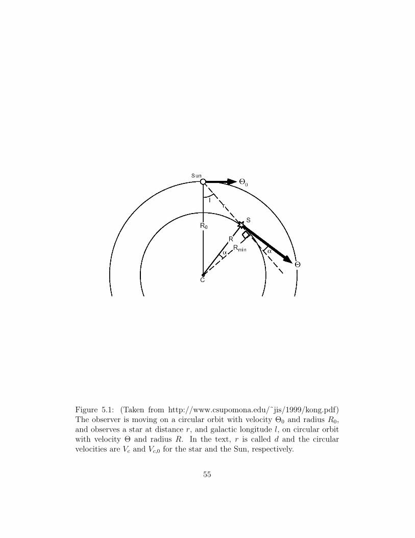
Figure 5.1: (Taken from http://www.csupomona.edu/˜jis/1999/kong.pdf)The observer is moving on a circular orbit with velocity Θ0 and radius R0,and observes a star at distance r, and galactic longitude l, on circular orbitwith velocity Θ and radius R. In the text, r is called d and the circularvelocities are Vc and Vc,0 for the star and the Sun, respectively.

55

Figure 5.2: A spiral pattern made out of stars will rapidly wind-up in a diskundergoing differential rotation.

56

Chapter 6

The Dark Halo

Measurements of the rotation curve from HI 21-cm emission, analysis ofthe motions of stars in the solar neighbourhood with Oort’s constants, andthe Oort limit, all suggest the presence of a large amount of invisible ‘darkmatter’ in the MW. Given such a startling conclusion, it may be a good ideato look for other evidence for dark matter in galaxy haloes.

6.1 High velocity stars

A number of high-velocity stars near the Sun have measured velocities1 upto v? ≈ 500km s−1. Their existence provides us with a probe of the galaxy’smass, if we assume that these stars are still bound to the MW: it means thatthe escape speed2 at the solar circle, ve > v?.

6.1.1 Point mass model

If we assume there is no dark halo, then it is easy to find a relation betweenthe circular velocity Vc and the escape speed ve. If we assume all mass M

1The quoted velocity is wrt to the centre of mass velocity of the MW. Do not confusethese with Oort’s high velocity stars, which are typically low mass, low metallicity stars inthe Galactic Halo. The velocities of Oort’s stars are of order 200km s−1. The present highvelocity stars are typically A-type stars, presumably born in the disk, that have acquiredtheir high velocity following a super nova explosion.

2Stars travelling at the local escape speed are just able to leave the potential well andescape to infinite.

57

of the MW is interior to the solar radius R3, then V 2

c = GM/R, and thepotential Φ = −GM/R = −V 2

c . The velocity of a star just able to escapefrom the gravitational well is the escape speed, ve. So since that star has zerototal energy,

0 = E =1

2v2

e + Φ =1

2v2

e − V 2c . (6.1)

So in this case, ve = 21/2 Vc ≈ 311km s−1 (Using Vc = 220km s−1.) So fora point mass model of the MW, these high velocity stars cannot be bound tothe MW – suggesting once more the presence of more mass in the outskirts ofthe MW than expected, given the rapid decrease in the distribution of light.

6.1.2 Parameters of dark halo

Given the failure of the point mass MW model, let’s assume there to be adark halo. In addition, let us assume the MW to be spherical, with a constantcircular speed Vc out to some radius R?. Since V 2

c = GM/R = constant, wehave that

M(R) =V 2

c R

Gwhen R < R?

=V 2

c R?

Gwhen R ≥ R? . (6.2)

Now the equation for the potential Φ is

dΦ

dR=GM

R2=V 2

c

R, (6.3)

for R ≤ R?. Integration gives Φ = constant − V 2c ln(R?/R). We can

determine the value of the constant at R = R?, since then Φ = −GM/R? =−V 2

c . Hence

Φ(R) = −V 2c [1 + ln(R?/R)] . (6.4)

Using Eq.(6.1) for the escape speed, we obtain

3R is the radius of the circular orbit around the MW, at the position of the Sun –the solar galacto-centric radius.

58

v2e = 2V 2

c [1 + ln(R?/R)] . (6.5)

For the Sun, R ≈ 8.5kpc, Vc = 220km s−1, ve ≥ 500km s−1, implyingR? ≥ 41kpc, hence

M(R = R?) ≥ 4.6× 1011M . (6.6)

Since the total luminosity of the MW is of order 1.4× 1010L (in the V-band), it means4 that the mass-to-light ratio is at least 30. Given that themass-to-light ratio of the MW stars is around 3 or so, our reasoning againsuggests that a dominant fraction of the MW mass is not in stars.

Another estimate of the MW mass comes from the motion of neighbouringgalaxies in the Local Group.

6.2 The Local Group

The MW is located in a rather average part of the Universe, away fromany dense concentrations of galaxies. The ‘Local Group’ consist of the MW,Andromeda (M31), and about 40 small, irregular galaxies, gravitationallybound to each other.

6.2.1 Galaxy population

The MW has a couple of small galaxies gravitationally bound to it, for ex-ample the Large and Small Magellanic Clouds. The Magellanic stream is astream of gas which originates from the Large Magellanic Cloud, which canbe traced over a significant fraction of the whole sky. It may result from thetidal forces exerted by the MW.

The Sagittarius Dwarf galaxy is the neighbouring galaxy closest to theMW. It was discovered as recently as 1994, having eluded detection sinceit happens to be at the other side of the MW bulge and therefore is hidingbehind a large amount of foreground stars. Sagittarius has ventured so closeto the MW that the tidal forces will probably tear it apart in the near future.Its discovery was actually hampered by its close proximity, since the largearea on the sky (∼ 8o × 2o) made it difficult to pick out against the bright

4Remember: we’ve only derived a lower-limit to the MW mass, hence a lower-limit tothe mass-to-light ratio.

59

MW foreground. Even away from the galactic plane (where dust obscurationlimits our view), new members of the LG continue to be identified. The studyof these small galaxies is exciting, since they allow us to constrain models forgalaxy formation and evolution.

The Andromeda galaxy M31 is about twice as bright as the MW, andis the brightest member of the Local Group (LG). It is very similar to theMW, and so also has its own set of small galaxies orbiting around it. Thesegalaxies, together with another 20 small galaxies, form the LG. M31 and theMW are by far the most massive galaxies in the LG.

The LG is almost certainly gravitationally bound to other nearby groups,and so does not really have a well defined edge. Galaxies in the outskirts ofthe LG may in fact belong to other groups.

The distribution of galaxies in the LG is rather untidy and lacks anyobvious symmetry. Most of the galaxies are found either close to the MW,or close to M31. There is a third, smaller condensation of galaxies, hoveringaround NGC 3109.

The motion M31 can be used to estimate the mass of the Local Group,using the Local Group timing argument.

6.2.2 Local Group timing argument

The dynamics of M31 and the MW can be used to estimate the total massin the LG. From the Doppler shifts of spectral lines, one can measure theradial velocity of M31 with respect to the MW5,

v = −118km s−1 . (6.7)

The negative sign means that Andromeda is moving toward the MW.This may be surprising, given that most galaxies are moving apart with thegeneral Hubble flow. The fact that Andromeda is moving toward the MWis presumably because their mutual gravitational attraction has halted, andeventually reversed their initial velocities. Kahn and Woltjer pointed out in1952 that this leads to an estimate of the masses involved.

Since M31 and the MW are by far the most luminous members of the LGwe can neglect in the first instance the others, and treat the two galaxies as

5What one measures is the radial velocity wrt to the Sun. Since the Sun is on a (nearly)circular orbit around the MW, one needs to correct the measured heliocentric velocity toobtain the radial velocity of Andromeda wrt the MW.

60

an isolated system of two point masses. Since M31 is about twice as brightas the MW, and given that they are so similar, it is presumably also abouttwice as massive. If we further assume the orbit to be radial, then Newton’slaw gives for the equation of motion

d2r

dt2= −GMtotal

r2, (6.8)

where Mtotal is the sum of the two masses. Initially, at t = 0, we can taker = 0 (since the galaxies were close together at the Big Bang).

The solution can be written in the well known parametric form

r =Rmax

2(1− cos θ)

t =

(R3

max

8GMtotal

)1/2

(θ − sin θ) . (6.9)

The distance r increases from 0 (for θ = 0) to some maximum value Rmax

(for θ = π), and then decreases again. The relative velocity

v =dr

dt=dr

dθ/dt

dθ=

(2GMtotal

Rmax

)1/2 (sin θ

1− cos θ

). (6.10)

The last three equations can be combined to eliminate Rmax, G andMtotal,to give

v t

r=

sin θ (θ − sin θ)

(1− cos θ)2. (6.11)

v can be measured from Doppler shifts, and r ≈ 710kpc from Cepheidvariables. For t we can take the age of the Universe. Current estimates of tare quite accurate6, but even using ages of the oldest MW stars, t ∼ 15Gyrgives an interesting result. Using these numbers, we can solve the previousequation (numerically) to find θ = 4.32 radians, assuming M31 is on its firstapproach to the MW7.

6From properties of the micro-wave background radiation.7Equation (6.11) has no unique solution for θ, since it describes motion in a periodic

orbit. On its first approach, θ should be the smallest solution to the equation.

61

Substituting yields Mtotal ≈ 3.66× 1012M, and hence for the MW mass,M ≈Mtotal/3

M ≈ 1.2× 1012M , (6.12)

comfortably higher than our lower limit Eq.(6.6).Since the luminosity of the MW (in the V band) is 1.4× 1010L, the cor-

responding mass-to-light ratio for the MW is around Γ = 100. Furthermore,the estimate of M is increased if the orbit is not radial, or M31 and the MWhave already had one (or more) pericenter passages since the Big Bang.

If all stars in the MW and M31 were solar mass stars, we would expectΓ = 1. Now even in the solar neighbourhood, most stars are less massivethan the sun, and so the mass-to-light ratio for the stars is about 3 or so8. Sothe very large mass inferred from the LG dynamics strongly corroborates theevidence from rotation curves and Oort’s constants, that most of the massin the MW (and presumably also in M31) is dark.

From these numbers, we can also estimate the extent R? of such a putativedark halo. If the the circular velocity Vc = 220km s−1 out to R?, then fromV 2

c = GM/R? we find

R? =GM

V 2c

≈ G 1012M

(220km s−1)2≈ 100kpc . (6.13)

If, as is more likely, the rotation speed eventually drops below 220km s−1,then R is even bigger. Hence the extent of the dark matter halo around theMW and M31 is truly enormous. Recall that the size of the stellar disk is oforder 20kpc or so, and the distance to M31 ∼ 700kpc. So the dark matterhaloes of the MW and M31 may almost overlap.

8Recall that the luminosity of stars scales with their mass quite steeply, L ∝ Mα, withα ≈ 5, and hence M/L ∝ M1−α. See your notes on stars, p. 34.

62

6.3 Summary

After having studied this lecture, you should be able to

• Show that in a point mass model of the MW, the high velocity starsare not bound.

• Estimate the parameters of a dark halo, assuming the high velocitystars are bound to the MW.

• Describe the properties of the Local Group in terms of the galacticcontent.

• Estimate the mass and extent of the dark halo of the MW from theLocal Group timing argument.

63

Chapter 7

Elliptical galaxies. I

Elliptical galaxies are spheroidal stellar systems with smooth luminosity pro-files which contain old, metal rich stars. They have a large range in sizes.Usually, rotation is unimportant in ellipticals, unlike for spirals. They oftencontain low density, very hot gas that emits X-rays. The properties of thishot gas, and also the stellar dynamics, suggest that also in ellipticals mostof the mass is in dark matter.

7.1 Luminosity profile

In contrast to spirals galaxies, elliptical have smooth surface brightness (SB)profiles, ellipsoidal in shape. The SB profile of some elliptical are shown inFigure (7.1). Note how in the center the isophotes are well defined and ellip-tical, whereas in the outer parts they become less smooth (noisier) becausethe SB decreases. Also note the presence of foreground MW stars.

A plot of the average surface brightness as function of radius for thesesame ellipticals is shown in Figure (7.2). The drawn line which fits the datawell, is an r1/4 fit, Eq. (3.2). Often, these profiles are plotted as SB vs r1/4 inwhich case the profile is a straight line, as in Figure (7.3). For most ellipticalsthis profile shape fits their SB-distribution well. A more general fit whichsometimes used, is I(r) ∝ exp[−(r/re)

1/n], where n = 4 corresponds to thede Vaucouleurs r1/4 fit.

Some of the giant elliptical galaxies that are invariably found in the cen-ters of big clusters of galaxies have an extended halo that is not fit well bythe de Vaucouleurs profile. Such galaxies are called cD galaxies. Fig. (7.4)

64

Figure 7.1: (Taken from astro-ph/0206097) Lines of constant surface bright-ness (isophotes) in the K band for four elliptical galaxies. In successiveisophotes, the surface brightness increases by 0.25 magnitudes.

65

arX

iv:a

stro

-ph/

0206

097

v1

6 Ju

n 20

02

0 5 10 15

15

15.5

16

16.5

17

17.5

18

18.5

19

19.5

Arp 156

a"

K m

ag (

arcs

ec)−

2

0 5 10 15 20 25 30 35

14

15

16

17

18

19

20

Arp 165

a"

K m

ag (

arcs

ec)−

2

0 2 4 6 8 10 12 14 16

15

15.5

16

16.5

17

17.5

18

18.5

19

19.5

20

Arp 193

a"

K m

ag (

arcs

ec)−

2

0 5 10 15 20 25 30

14.5

15

15.5

16

16.5

17

17.5

18

18.5

19

19.5

20

Arp 221

a"

K m

ag (

arcs

ec)−

2

0 5 10 15 20 25 30 35 40 45

13

14

15

16

17

18

19

20

Arp 222

a"

K m

ag (

arcs

ec)−

2

0 10 20 30 40 50

13

14

15

16

17

18

19

Arp 225

a"

K m

ag (

arcs

ec)−

2

Figure 7.2: (Taken from astro-ph/0206097) Surface brightness as function ofdistance to the center. The drawn line is the best r1/4 fit.

66

Figure 7.3: Luminosity profile for galaxy NGC 3379 (open symbols) and r1/4

fit (drawn line). Taken from de Vaucoleurs & Capaccioli, ApJS 40, 1979.

67

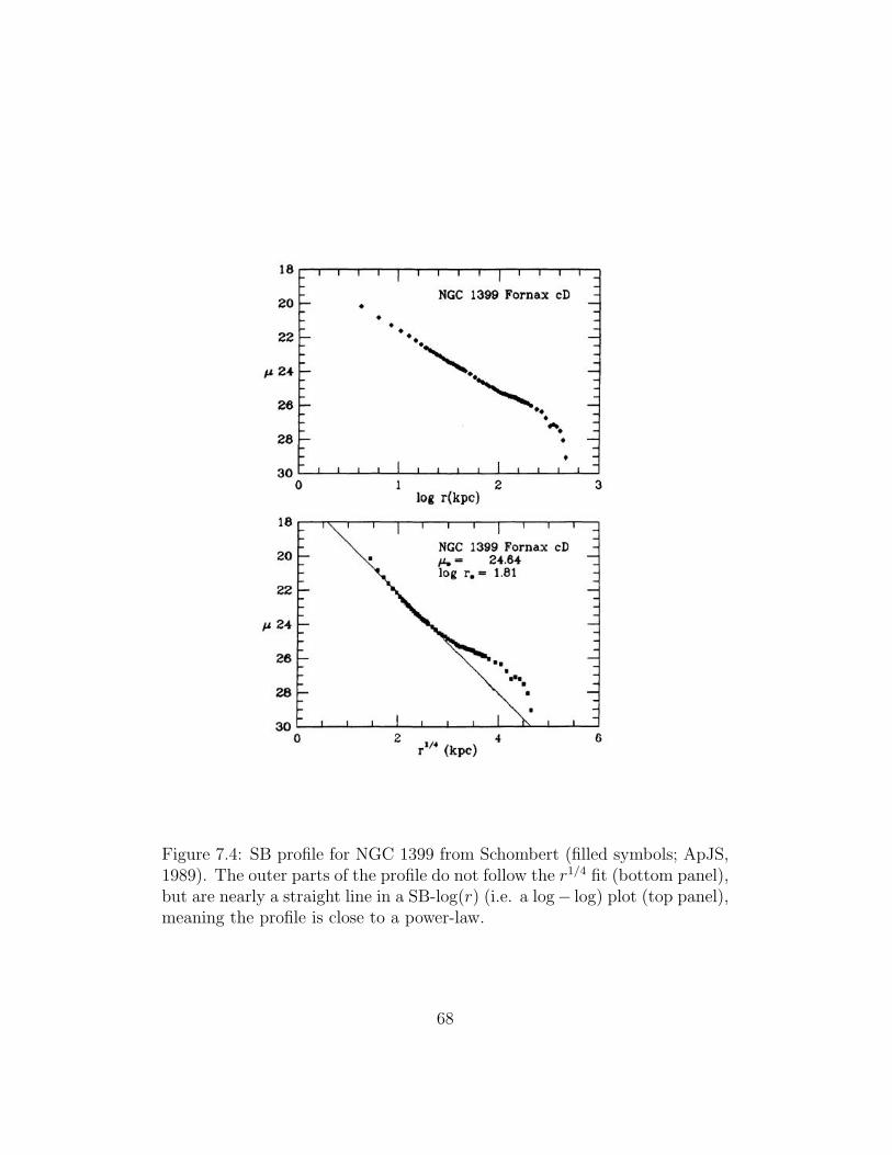
Figure 7.4: SB profile for NGC 1399 from Schombert (filled symbols; ApJS,1989). The outer parts of the profile do not follow the r1/4 fit (bottom panel),but are nearly a straight line in a SB-log(r) (i.e. a log− log) plot (top panel),meaning the profile is close to a power-law.

68

Figure 7.5: Image of NGC 1399 with smooth, best fit r1/4 profile subtracted(Bridges et al., AJ 101, 469 (1991). The centre of NGC 1399 is at the left, theobject toward the top right is another galaxy in the galaxy cluster. The otherextended objects in the image are other galaxies. Clearly seen are hundredsof high SB unresolved objects, which are GCs in the halo of NGC 1399.

69

show the profile of NGC 1399, which is the cD galaxy in the nearby Fornaxcluster of galaxies. This very extended halo of stars is truly enormous: itcan be traced to around a Mpc . Even though the distance to Fornax islarge, it means that the extent on the sky of NGC 1399 is about the size ofthe moon! This gigantic size has prompted the suggestion that may be weshould associate such a halo with the cluster of galaxies, rather than with anyindividual galaxy. This suggestion has some support from the observationsof some clusters where we observe a faint halo, but without a galaxy in thecenter!

Es also have many globular clusters. Figure (7.5) is an image of NGC 1399,where an r1/4 fit to the SB-profile of the galaxy has been subtracted. Clearlyvisible are 100s of high SB objects, indistinguishable on this plate from fore-ground stars, which are in fact GCs in the halo of the galaxy. The GCluminosity function (i.e., the number of clusters as function of their mag-nitude) has been used as a standard candle: by measuring the luminosityfunction of GCs of a galaxy, and comparing it to the luminosity function ofa galaxy with known distance, one can obtain a distance estimate.

Why do ellipticals have an r1/4 SB-profile? As I explained earlier, thereseems to be a strong connection between the density of galaxies (in thesense of how many galaxies you find per Mpc3 in a given region, say) andtheir types: high density regions invariably contain a much larger fractionof Es than low density regions, where Ss dominate. So, may be interactionsbetween galaxies have something to do with it?

Recent numerical simulations of collisions between two spiral galaxies doproduce objects with SB-profiles not too different from r1/4 appropriate foran E. And although this is a good hint that we’re on the right track, in fact,also in the simulations we don’t really know why this is. In a famous paper,Donald Lynden-Bell suggested that during a galaxy merger, the gravitationalpotential Φ which the stars feel, changes very rapidly and this might producea characteristic density profile1. He termed this process violent relaxation.And so the suggestion is that, as (predominantly spiral) galaxies fall intogalaxy clusters, they will violently interact with other galaxies, transformingthem somehow into Es. And although this is certainly an important piece of

1rather, a characteristic distribution function, the density of stars in six-dimensionalposition and velocity space.

70

the puzzle, it can’t be the whole story, because the stellar populations of Esand Ss differ.

7.2 Stellar populations and ISM

Stars in Es tend to be older and more metal rich than those in Ss, and as aconsequence Es are redder than Ss. You can easily understand why this is so.We discussed this before: if the atmosphere of a star contains more metals,then the dust and the gas will scatter preferentially the blue light hence thestars appears redder. That’s one. Secondly, if you have young stars in astellar population, then the more massive stars may still be alive2, and theseare hot and hence blue. So when a given stellar population gets older, it willbecome redder as well. And in an E galaxy, both effects occur.

The fact that a stellar population appears blue either because it is young,or because it is metal poor, is called the age-metallicity degeneracy: just ob-serving the colour of a population, you cannot tell a young but metal richpopulation apart from an old but metal poor one. To make sure, you haveto have independent constraints on th metallicity Z, for example from stellarspectra, or, the astronomer’s favourite, from HII regions.

Dust and gas Although I said that a characteristic difference between Es andSs is that Es don’t contain dust or gas, and have no star formation, this isof course not complete true, they usually have some, but much less than Ss.Many Es contain strong dust lanes, the Sombrero galaxy is a beautiful exam-ple (Fig. 7.6). Often, there is almost no connection between the orientationof the dust lane, and any other of the galaxy’s parameters. It is thought thatsuch dust lanes are evidence that the E recently swallowed a small galaxy. Infact, one sometimes observes very faint rings of stars around an E, and alsothis could be the result of ‘galactic cannibalism’. A good example is shownin Figure (7.7).

2Recall that massive stars have short lifetimes.

71

Figure 7.6: Image of the ‘Sombrero’ galaxy, with its striking dust lane.

72

Figure 7.7: Image of NGC 3923 taken by David Malin. Severalfaint shells of stars appear in the outer parts of the galaxy. (seehttp://www.ast.cam.ac.uk/AAO/images/general/ngc3923.html)

73

7.3 X-rays

Elliptical galaxies emit X-rays. I want to briefly discuss why, how X-rays areobserved, and what we can learn from them.

Fortunately for us, the earth’s atmosphere blocks X-rays. Unfortunatelyfor astronomers, this means we need to be above the atmosphere, in a bal-loon, rocket or satellite, to observe extra-solar X-rays.

How does one built an X-ray telescope? X-rays do not reflect off mir-rors the same way that visible light does. Because of their high energy,X-ray photons penetrate into the mirror in much the same way that bul-lets slam into a wall. Likewise, just as bullets ricochet when they hit awall at a grazing angle, so too will X-rays ricochet off mirrors. Theseproperties mean that X-ray telescopes must be very different from opticaltelescopes. Basically, they contain many almost parallel plates, that gen-tly nudge the incoming X-rays into the new direction you want them to goin. See http://chandra.harvard.edu/xray astro/ for a nice diagram and moredetailed info.

The sun (we’re really close!) was the first source to be detected in the X-rays, in 1949. The technology improved in great leaps, and it came somewhatas a surprise to detect X-rays from Es that were not associated with pointsources. Why am I talking about point sources? Recall from the stellarpart of the course the concept of X-ray binary. In these binary stars, hotgas associated with mass transfer radiates in the X-ray band. Such (binary)stars are also seen in Es. But subtracting these sources from the X-ray image,we still detect extended X-ray emission from the galaxy. The process thatproduces them is called thermal bremsstrahlung.

7.3.1 Thermal bremsstrahlung

How are the X-rays produced in this hot gas? Since the gas temperature isvery high, most elements are highly ionised, and so the gas is really a hotplasma. The negatively charged electrons in this plasma experience a forcewhen they pass close to an ion, and an accelerating charge emits electro-magnetic dipole radiation: this is the radiation that we observe. Since theelectron looses energy in the encounter, it will slow down. Hence the name

74

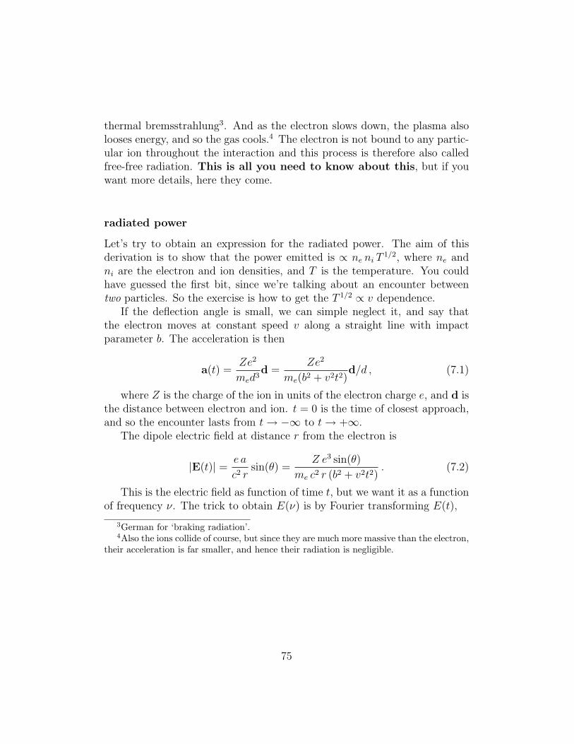
thermal bremsstrahlung3. And as the electron slows down, the plasma alsolooses energy, and so the gas cools.4 The electron is not bound to any partic-ular ion throughout the interaction and this process is therefore also calledfree-free radiation. This is all you need to know about this, but if youwant more details, here they come.

radiated power

Let’s try to obtain an expression for the radiated power. The aim of thisderivation is to show that the power emitted is ∝ ne ni T

1/2, where ne andni are the electron and ion densities, and T is the temperature. You couldhave guessed the first bit, since we’re talking about an encounter betweentwo particles. So the exercise is how to get the T 1/2 ∝ v dependence.

If the deflection angle is small, we can simple neglect it, and say thatthe electron moves at constant speed v along a straight line with impactparameter b. The acceleration is then

a(t) =Ze2

med3d =

Ze2

me(b2 + v2t2)d/d , (7.1)

where Z is the charge of the ion in units of the electron charge e, and d isthe distance between electron and ion. t = 0 is the time of closest approach,and so the encounter lasts from t→ −∞ to t→ +∞.

The dipole electric field at distance r from the electron is

|E(t)| = e a

c2 rsin(θ) =

Z e3 sin(θ)

me c2 r (b2 + v2t2). (7.2)

This is the electric field as function of time t, but we want it as a functionof frequency ν. The trick to obtain E(ν) is by Fourier transforming E(t),

3German for ‘braking radiation’.4Also the ions collide of course, but since they are much more massive than the electron,

their acceleration is far smaller, and hence their radiation is negligible.

75

E(ν) ≡∫ ∞

−∞E(t) exp(2π iν t)dt

=Ze3 sin(θ)

mec2 r

∫ ∞

−∞

exp(2π iν t)

b2 + v2t2dt

=Ze3 sin(θ)

mec2 r

1

b v

∫ ∞

−∞

exp(2π ix(ν b/v))

(1 + x2)dx

=Ze3 sin(θ)

mec3b2v2

π

bvexp(−2πν b/v) . (7.3)

Along the way, I’ve introduced the variable x = vt/b. The integral∫exp(2πxα)/(1 + x2) dx = some function of α is a little tricky to perform,

and I don’t expect you to be able to do it. What is important is to note thatthis change of variables gives rise to a factor 1/bv .

Now we’re done, because it means that the power radiated by this singleelectron per unit frequency is

dW

dν∝

∫E2(ν) dΩ ∝ 1

(b v)2exp(−4πν b/v) . (7.4)

So the spectrum is independent of ν for low frequencies ν v/b, andcuts off exponentially for large ν. Now the number of encounters with impactparameter between b and b+ db, in time dt is ne2πb dbvdt, and so this givesthe power as

dW

dν dt dV∝ ne ni v

−1 exp(−4πν b/v) ∝ ne ni T−1/2 exp(−4πν b/v) . (7.5)

So the origin of the 1/v is that the energy radiated per encounter ∝ 1/v2

whereas as the rate of encounters is ∝ v.To obtain the final result, we still need to integrate over the impact pa-

rameter b, and average over all impact velocities v (for example by assuminga Maxwell-Boltzmann distribution for v). The result is that the total poweremitted is

power ∝ ne ni T1/2 . (7.6)

Notice that the total power is much more dependent on the density ofthe gas (∝ density squared), than on its temperature (∝ T 1/2)

76

7.3.2 Spectrum

On top of the thermal bremsstrahlung emission spectrum, observed X-rayspectra also exhibit spectral lines. Given the high temperature of the gas,it won’t come as a surprise that we observe lines of highly ionised species– Fe-lines are especially important in the wave-bands observed by modernX-ray telescopes. And just as we did for HII regions, we can try to constrainthe physical conditions in the hot gas, by modelling the relative strength ofdifferent transitions. This is one way to determine the temperature T of thehot gas.

7.4 Evidence for dark matter from X-rays

An important application of X-ray observations is to probe the gravitationalpotential of the galaxy, and hence infer its density distribution. Consider athin shell of hot gas. The gravitational force due to mass enclosed by theshell (consisting of stars, gas and dark matter) will pull the shell inward. Atthe same time, if the pressure decreases outward, then the pressure gradientwill try to push the shell outward. In hydrostatic equilibrium, these forcesbalance. By estimating the pressure gradient from X-rays, we can infer thegravitational force and hence look for evidence for dark matter. Let’s assumefor simplicity that the elliptical galaxy is spherically symmetric.

Let M(< r) be the mass inside the shell of radius r (consisting of stars,gas and dark matter: M = M? + Mgas + Mdm), and dr its thickness Thegravitational force on the shell is

Fg(r) =GM(< r)Ms

r2, (7.7)

where Ms = 4πr2ρgas(r)dr is the mass of the shell.Let p(r) be the pressure in the hot gas. The pressure force on a surface

is p(r) times the surface area, 4πr2. The net outward force is the differencebetween the outward and inward forces:

Fp(r) = 4πr2(p(r)− p(r + dr)) = −4πr2dp

drdr (7.8)

where the pressure was expanded in a Taylor series. Combining the last threeequations gives

77

GM(< r)

r24πr2ρgas(r)dr = −4πr2dp

drdr , (7.9)

henceGM(< r)

r2= − 1

ρgas(r)

dp

dr, (7.10)

or alternatively in terms of the gravitational potential Φ

∇Φ = −∇p/ρgas . (7.11)

This should look familiar from hydrostatic equilibrium in stars!

By modelling the spectrum as function of position we can determine T (r),and since the X-ray intensity∝ ρ2

gasT1/2, we can also determine ρgas(r). Hence

p ∝ rhogasT , and so we have determined the rhs of Eq.(7.11). From that,one can reconstruct the gravitational potential, and hence infer the massdistribution.

The temperature T is observed to remain approximately constant, inwhich case we can obtain an approximate expression for the density profile.The pressure is

p =kB T

µmp

ρgas . (7.12)

If we take T constant then the rhs of Eq. (7.10) becomes− kB Tµmp

d ln(ρgas)/dr,

and hence

GM(< r) = − kBT

µmp

r2d ln ρgas

dr. (7.13)

Taking the derivative of both sides with respect to r, gives

G4πr2ρtot = − kBT

µmp

d

dr(r2d ln ρgas

dr) , (7.14)

since dM(< r)/dr = 4π r2 ρtot. ρtot is the total mass density, i.e. due tostars, gas and dark matter.

Now assume that the gas density and total mass density are proportional,ρgas ∝ ρtotal, and try a solution of the form ρtotcl = ρ0 (r0/r)

β. Substitution

78

shows that this is indeed a solution when β = 2, in which case

ρtot(r) =kB T

2π Gµmp

r−2 . (7.15)

So a measurement of T can constrain the total mass density ρtot. Esti-mating the stellar mass density from the luminosity, the gas density from theX-ray emissivity, we find ρdm = ρtotal− ρ?− ρgas. More detailed modelling ofthis type confirms that also elliptical galaxies have most of their mass in theform of dark matter.

79

7.5 Summary

After having studied this lecture, you should be able to

• describe the surface brightness profiles of Es in terms of the de Vau-couleurs profile.

• explain why we think that this profile results from galaxy encounters.

• recall that Es have typically hundreds of GCs.

• explain why dust lanes in Es and shells of stars around Es are thoughtto be evidence for galactic cannibalism.

• contrast the stellar population and ISM of Es with those of Ss.

• describe how X-rays are detected, and explain the process with whichX-rays are produced in the hot gas in Es. (But not be able to recallthe equation, or reproduce the calculation.)

• explain how X-ray observations can be used to infer the gravitationalpotential in Es.

80

Chapter 8

Elliptical galaxies. II

This chapter is a bit harder, with more mathematics than I would like touse. I do not expect you to be able to reproduce all these derivations, onlythe ones stressed in the Summary. The aim of this chapter is twofold: (i)explain why you can derive fluid-like equations to describe the structure ofellipticals, and (ii) use these fluid equations to explain why elliptical areelliptical in shape.

We’ve seen that the stars in spiral disks are all on nearly circular orbits.Although some of the smaller Es sometimes rotate as well, the angular mo-mentum of stars is not sufficient to balance gravity. So we need to look foranother mechanism to prevent collapse. Basically, it’s the velocity dispersionof the stars that balances gravity, much like it is a pressure gradient in thegas that balances gravity in a star. For this reason, Es (but also spiral bulges,and globular clusters for example) are called hot stellar systems.

The Jeans’s equations relate the stellar velocity dispersion, σ2ij = 〈(vi −

〈vi〉)(vj − 〈vj〉)〉 with the gravitational potential of the system, and are thestellar analogue of the equation of hydrostatic equilibrium ∇Φ = −∇p/ρ ina star. They do not describe the properties of the orbits of a single star, butrather assume one can use averaged properties. To investigate whether suchan approach makes sense, I first need to introduce the concept of relaxationtime.

81

8.1 Relaxation in stellar systems

As a star moves through a stellar system, it will feel the gravitational forcedue to all other stars. Is the motion of this star mainly determined by theaverage gravitational force of all other stars combined, or is it mostly sensitiveto the force due to near stars?

To see that this would make a huge difference, consider the case wherea single star (a test particle) moves through a smooth density distributionwith spherically symmetric density distribution ρ(r), where r = |r|. In sucha time-independent potential both the angular momentum, L = m r × v,and energy, E = v2/2 + Φ, of the star will be conserved along its orbit. Nowsuppose such a density distribution to be represented by a finite number ofstars. As our test star moves along its orbit, it will be deflected by encounterswith these other stars. In such a situation, neither L nor E will be conserved,and so the properties of its orbit will change in time. Clearly, the longer thestar orbits in this density distribution, the more E will differ from its initialvalue. The relaxation time TE is a measure of how long the star remembersits initial energy. We will see that the more stars are there in the galaxy,the longer is the relaxation time. You might have expected this, since for aninfinite number of stars, the density is smooth, L and E are constant, andhence TE →∞.

To estimate TE, we will compute the change in energy ∆E of a star dueto a single encounter with another star, as function of the impact param-eter b and impact velocity v (the velocity at infinity, before the encounterstarted), and then sum over encounters. This derivation was first done byChandrasekhar, the derivation here is slightly different from BT (p. 188).

Let’s compute the change in velocity δv of this star. Because we wantto treat the case where the effect of encounters is small, we’ll approximatethe orbit as a straight line, traversed with constant velocity v. The forceperpendicular to the orbit is

F⊥ =Gm2

b2 + (vt)2cos(θ) ≈ Gm2

b2

[1 + (

vt

b)2

]−3/2

, (8.1)

where I’ve assumed equal mass stars. The approximation cos(θ) = b/r ≈b/vt is valid for b small. Combined with Newton’s law

82

mv⊥ = F⊥ , (8.2)

yields the net change |δv⊥| over a single encounter:

|δv⊥| ≈Gm

bv

∫ ∞

−∞(1 + s2)−3/2 ds =

2Gm

b v. (8.3)

Thus the change is roughly equal to the force at closest approach, Gm/b2,times the time this force acts, ∆t ∼ b/v. Because of symmetry, encountersare equally likely to change the velocity in the positive direction, as in thenegative direction. Therefore the mean change 〈δv⊥〉 = 0. We will thereforeconsider the rate of change of δv2

⊥.

To compute the rate of change of δv2⊥, due to many encounters, proceed as

follows. Suppose the test star moves with velocity v through a stellar systemwith radius R, and (uniform) number density of stars, n. When travellingfor a time δt, the number of encounters with impact parameter between band b+ db, is simply the volume of the cylindrical shell, dV = 2π b db × vδt,times the number density of stars, n. Here, vδt is the length of the cylinder,2π b db is the surface area of the shell. Since each of these encounters leadsto a change in velocity squared by an amount δv2

⊥, we find for the rate ofchange

d2δv2⊥

dt db= n v 2π b × (

2Gm

b v)2 . (8.4)

This is the product of the rate of encounters, n v 2π bdb, with the velocitychange per encounter. Now we can integrate over impact parameter to obtainfor the rate of change in velocity

dδv2⊥

dt=

∫ ∞

0

n v 2π b (2Gm

b v)2 db = 2π nv (

2Gm

v)2

∫ ∞

0

db

b. (8.5)

Unfortunately this integral diverges, both at small impact parameters(which are few in number, but cause large velocity changes), and at largeimpact parameters (which cause small velocity changes yet are very numer-ous). How to overcome this divergence?

83

For a real stellar system, there cannot be encounters with impact param-eter larger than the size R of the system. For the smallest impact parameterb, we can take bmin = Gm/v2, for which the change in velocity is comparableto the initial velocity (cfr.Eq. 8.3). Recall that our derivation assumed smallchanges anyway. With this caveat in mind we replace the previous equationby

dδv2⊥

dt≈ 2π nv (

2Gm

v)2

∫ R

bmin

db

b= 2π nv (

2Gm

v)2 ln(

R

bmin

) . (8.6)

We can simplify this by assuming that the stellar system is in virial equi-librium, in which case the kinetic energy of all stars combined, K ∼ N mv2/2is half of the potential energy, U ∼ G (N m)2/R, where m is the mass of astar. Therefore

v2 ≈ GNm

R. (8.7)

Combining this with the expression for bmin it is easy to show thatR/bmin =N , the total number of stars.

So far we have computed the rate of change of the velocity. To judgewhether the change of velocity is large or small, we can multiply the ratewith the crossing time of the system, tcr ≡ R/v. It is a measure of how longit takes to cross the stellar system, on average. The velocity change duringa single crossing of the stellar system is therefore

δv2⊥ ∼

dδv2⊥

dttcr = 2π nv (

2Gm

v)2 ln(N)× R

v

=6 ln(N)

Nv2 . (8.8)

The first line combines Eq.(8.6) with our finding R/bmin = N and thedefinition of the crossing time. The second step assumes virial equilibrium,Eq. (8.7). We are finally in a position to define the relaxation time Trelax,as the time it takes for encounters to change the velocity by order of itself,hence

v2

Trelax

≡ dδv2⊥

dt=

6 ln(N)

N

v2

tcr(8.9)

84

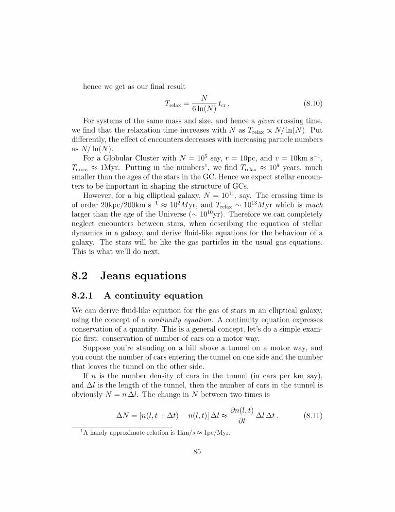
hence we get as our final result

Trelax =N

6 ln(N)tcr . (8.10)

For systems of the same mass and size, and hence a given crossing time,we find that the relaxation time increases with N as Trelax ∝ N/ ln(N). Putdifferently, the effect of encounters decreases with increasing particle numbersas N/ ln(N).

For a Globular Cluster with N = 105 say, r = 10pc, and v = 10km s−1,Tcross ≈ 1Myr. Putting in the numbers1, we find Trelax ≈ 109 years, muchsmaller than the ages of the stars in the GC. Hence we expect stellar encoun-ters to be important in shaping the structure of GCs.

However, for a big elliptical galaxy, N = 1011, say. The crossing time isof order 20kpc/200km s−1 ≈ 102Myr, and Trelax ∼ 1013Myr which is muchlarger than the age of the Universe (∼ 1010yr). Therefore we can completelyneglect encounters between stars, when describing the equation of stellardynamics in a galaxy, and derive fluid-like equations for the behaviour of agalaxy. The stars will be like the gas particles in the usual gas equations.This is what we’ll do next.

8.2 Jeans equations

8.2.1 A continuity equation

We can derive fluid-like equation for the gas of stars in an elliptical galaxy,using the concept of a continuity equation. A continuity equation expressesconservation of a quantity. This is a general concept, let’s do a simple exam-ple first: conservation of number of cars on a motor way.

Suppose you’re standing on a hill above a tunnel on a motor way, andyou count the number of cars entering the tunnel on one side and the numberthat leaves the tunnel on the other side.

If n is the number density of cars in the tunnel (in cars per km say),and ∆l is the length of the tunnel, then the number of cars in the tunnel isobviously N = n∆l. The change in N between two times is

∆N = [n(l, t+ ∆t)− n(l, t)] ∆l ≈ ∂n(l, t)

∂t∆l∆t . (8.11)

1A handy approximate relation is 1km/s ≈ 1pc/Myr.

85

Assuming there is no other exit, this is also the change between thenumber of cars entering and leaving the tunnel,

∆N = [n(l, t)l(l, t)− n(l + ∆l, t)l(l + ∆l, t)] ∆t ≈ −∂n(l, t) l(l, t)

∂l∆l∆t .

(8.12)The first term n(l, t)l(l, t) ∆t is the number of cars entering the tunnel

in time ∆t, the second term is how many are leaving in that time. l(l, t)obviously denotes the speed of the cars.

Combining these two equation, we get the following continuity equation:

∂n(l, t)

∂t+∂n(l, t) l(l, t)

∂l= 0 . (8.13)

A little bit of thought shows that, in a N-dimensional case (spaceshipsthrough a worm-hole?), the more general equation would be

∂n(l, t)

∂t+∂n(l, t) l(l, t)

∂l= 0 , (8.14)

so there is a partial derivative ∂/∂li for every Cartesian coordinate li,and n is multiplied by li in the second term, which is the velocity of thespaceships in the i-direction.

8.2.2 Boltzmann’s equation

We’re interested in finding an equation that describes the distribution ofstars in a galaxy. So we want to know is how many stars there are in asmall volume dx around a position x, that have velocity in a small intervaldx around a given velocity x. This density of stars, f(x, x, t), is called thedistribution function. If we don’t care about the velocity of stars, then wecan integrate f over all velocities, to obtain the density of stars,

n(x, t) =

∫f(x, x, t) dx . (8.15)

Now we only have to realise that stars acts as our cars on the motor way,and hence f should satisfy the continuity equation (8.14). The way to doit is to substitute for the l coordinates in that equation the positions andvelocities of the stars,

86

l ≡ (x,v)

l ≡ (v, v) = (v,−∇Φ) , (8.16)

where I’ve written −∇Φ for the gravitational acceleration v of the star.So this l vector has 6 coordinates, lα = x for α = 1 → 3, and lα = v for

α = 4 → 6. Now these coordinates are very special, since

6∑α=1

∂lα∂lα

=3∑

i=1

(∂vi

∂xi

+∂vi

∂vi

)

=3∑

i=1

− ∂

∂vi

(∂Φ

∂xi

)= 0 . (8.17)

Here, ∂vi/∂xi = 0 since the positions and velocities of the stars are in-dependent variables, and the second term is zero because the gravitationalacceleration ∂Φ/∂xi does not depend on velocity.

We can use this equation to simplify the continuity equation, and toobtain

∂f

∂t+

6∑α=1

lα∂f

∂lα= 0 . (8.18)

Rewriting in terms of positions and velocities, we obtain the collisionlessBoltzmann equation,

∂f

∂t+

3∑i=1

(vi∂f

∂xi

− ∂Φ

∂xi

∂f

∂vi

)= 0 . (8.19)

or in vector notation

∂f

∂t+ v · ∂f

∂r−∇Φ · ∂f

∂v= 0 . (8.20)

87

8.2.3 Moments of the Boltzmann equation

Although the collisionless Boltzmann equation (CBE for short) provides uswith a complete description of the stellar dynamics problem, it is ratherunwieldy for practical applications. The Jeans equations, which give a clearerphysical picture of what is going on, are moments of the Boltzmann equation.Here is how to obtain them.

Suppose we integrate Eq. (8.19) over all velocities. The first term willbecome ∫

∂f(r,v, t)

∂tdv =

∂

∂t

∫f(r,v, t) dv ≡ ∂n(r, t)

∂t. (8.21)

The integral of the distribution function over velocities, n ≡∫f dv is

just the density of stars. And we’re allowed to interchange the integral overvelocities, with the derivative wrt time, since the range of velocities overwhich we integrate does not depend on t.

Integrating the second term, gives∫vi∂f

∂xi

dv =∂

∂xi

∫vi f dv ≡

∂(nvi)

∂xi

, (8.22)

where I’ve introduced the mean velocity vi as

n vi =

∫vi f dv . (8.23)

Now the last term is zero, since∫ ∞

−∞

∂f

∂vi

dvi = f |vi=+∞vi=−∞ , (8.24)

since there are no stars with infinite velocity.And so the first moment of the CBE is a continuity equation for the

density,

∂n

∂t+∂(nvi)

∂xi

= 0 . (8.25)

Now the second moment is what we’re after. The trick is to first multiplythe CBE with vj, and then integrate over all velocities. The calculationproceeds exactly as for the density, and the result is after a bit of algebra:

88

n∂vj

∂t+ n vi

∂vj

∂xi

= −n ∂Φ

∂xj

−∂n σ2

ij

∂xi

. (8.26)

where

σ2ij ≡ vivj − vivj . (8.27)

This was a lot of mathematics to come to a simple equation: suppose thesystem is in a steady state, ∂/∂t=0, and there are no streaming motions, sothat vi = 0. Then the previous equation simplifies to

∂Φ

∂xj

= − 1

n

∂nσ2ij

∂xi

. (8.28)

This is a more general version for the equation of hydrostatic equilibrium.To see this, note that the matrix σij is symmetric: σij = σji. For suchsymmetric tensors, we can always rotate the coordinate system such thatthe tensor becomes diagonal, i.e. σ2

ij = 0 for i 6= j. Now, suppose that thevelocities are isotropic, so that σxx = σyy = σzz ≡ σ2. Then we find that

∂Φ

∂xj

= − 1

n

∂nσ2

∂xj

. (8.29)

which is exactly the same as the equation for hydrostatic equilibrium, ifnσ2 is identified with the pressure p. Because of this analogy, the tensor nσ2

ij

is called the pressure tensor.

In conclusion: the behaviour of collisionless stellar systems is similar tothat of self-gravitating gas spheres. The role of temperature is taken overby that of the stellar velocity dispersion. It is the high velocity dispersionof the stars in an elliptical (and also in the bulge of spirals), which balancesthe gravitational pull. Since the required velocities are so high, such systemsare called ‘hot stellar systems’. Recall that in disk galaxies, it is the orderedmotion of the stars – i.e. the rotation of the disk – which supports thesystem against gravity. Such systems are dynamically cold, i.e. the stellarvelocity dispersion is small compared to the streaming motions. For disks,the ‘velocity dispersion’ refers to the small velocities that stars have withrespect to their ‘local standard of rest’ (10s of km s−1), versus the rotationalvelocity of the disk, 200km s−1.

89

In a gas the pressure is isotropic and hence stars are spherical. In contrastin stellar systems, the pressure tensor nσ2

ij is in general not isotropic, and sothe pressure gradient can be larger in one direction (x, say) than in anotherdirection (y). So even if the potential is spherical, the stellar distributionmay be more extended in x than in y, and the system will be elliptical inshape.

90

8.3 Summary

After having studied this lecture, you should be able to

• to derive an estimate for the stellar dynamical relaxation time in aspherical system of N stars.

• explain why we can describe the dynamics of elliptical galaxies in termsof fluid equations.

• explain the difference in dynamics between an elliptical (hot stellarsystem) and a spiral (cold, rotating stellar system)

• explain what is a continuity equation, and derive the collisionless Boltz-mann equation, Eq.(8.20), stating the underlying assumptions.

• explain that the ellipticity of ellipticals does not results from rotation,but from the anisotropy of the pressure tensor.

91

Chapter 9

Groups and clusters of galaxies

Galaxies are not distributed homogeneously in the Universe. Some regions inthe Universe have a galaxy density (i.e. the number of galaxies per Mpc−3)significantly lower than the mean, and some a significantly higher density.The main reason for this is that gravity amplifies small inhomogeneities: ifa region is slightly denser than its surroundings (for example a group ofgalaxies), it will tend to attract more matter than the surrounding regions,and hence become even more massive (turn into a galaxy cluster, say). Thisis the essence of hierarchical structure formation: small structures mergetogether to make more massive one.

The galaxies huddle together in groups of a few galaxies – such as theMW and M31 in the Local Group – and some are in clusters with hundreds ofgalaxies. The groups and clusters themselves are clustered in super clusters(i.e. clusters of clusters). But there are no clusters of super clusters: on suf-ficiently large scales the Universe is not a fractal but becomes homogeneous.

9.1 Introduction

Recall that the MW, M31, and some 40 small irregular galaxies within 2Mpcor so from the MW, are part of a gravitationally bound system, called theLocal Group. Several other such bound groups occur at larger distancesfrom the MW, and searches over larger volumes have revealed the existenceof 1000s of such groups of galaxies.

Within about 20Mpc from the MW are several clusters of galaxies, con-

92

taining 10s of large galaxies, and hundreds of smaller ones each. The Virgocluster of galaxies contains the big elliptical M87. We already discussed thebig cD galaxy NGC1399 at the centre of the Fornax galaxy cluster. The typi-cal total mass of these clusters is estimated at around 1014M. At 90Mpc wefind the Coma cluster of galaxies, with a mass of may be as large as 1015M.Clusters such as Coma contain the most massive known galaxies.

In the 1950s, George Abell and collaborators eye balled photographicplates to look for rich clusters of galaxies, by finding regions with a largeover density of galaxies. He found some 4500, and ranked them from poorto rich, according to the number of galaxies they had. Paul Hickson laterperformed a similar exercise looking for ‘Hickson’ compact galaxy groups.

Clusters of galaxies are the most massive virialised structures in the Uni-verse. Their crossing time1 is sufficiently small that each galaxy has had theopportunity to cross the system several times, and hence the system has hadtime to dynamically relax to a near equilibrium situation, i.e. the system isclose to being in virial equilibrium. Although more massive bound systemsexist, these have crossing times which are so large that, given the age of theUniverse, they have not had time to become dynamically relaxed.

9.1.1 Evidence for dark matter from galaxy motions

Evidence for the existence of dark matter in galaxy clusters dates from the1930s. The Swiss astronomer Fritz Zwicky used the velocity dispersion ofgalaxies in clusters as determined from Doppler shifts to estimate their dy-namical mass. Suppose all galaxies have the same mass m, then the kineticenergy of the system of N galaxies is

K =1

2

∑mv2 =

1

2M σ2 , (9.1)

where M = N m is the total mass of the cluster galaxies, and the velocitydispersion σ2 is defined as

σ2 =

∑mv2

M. (9.2)

The potential energy in the system is of order

1If v is the typical velocity of a galaxy in a cluster of galaxies, and R is the radius ofthe cluster, then the crossing time Tcr = R/v, i.e. it is the typical time a galaxy takes tocross the cluster once.

93

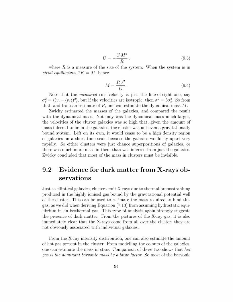
U = −GM2

R, (9.3)

where R is a measure of the size of the system. When the system is invirial equilibrium, 2K = |U | hence

M =Rσ2

G. (9.4)

Note that the measured rms velocity is just the line-of-sight one, sayσ2

z = 〈(vz−〈vz〉)2〉, but if the velocities are isotropic, then σ2 = 3σ2z . So from

that, and from an estimate of R, one can estimate the dynamical mass M .Zwicky estimated the masses of the galaxies, and compared the result

with the dynamical mass. Not only was the dynamical mass much larger,the velocities of the cluster galaxies was so high that, given the amount ofmass inferred to be in the galaxies, the cluster was not even a gravitationallybound system. Left on its own, it would cease to be a high density regionof galaxies on a short time scale because the galaxies would fly apart veryrapidly. So either clusters were just chance superpositions of galaxies, orthere was much more mass in them than was inferred from just the galaxies.Zwicky concluded that most of the mass in clusters must be invisible.

9.2 Evidence for dark matter from X-rays ob-

servations

Just as elliptical galaxies, clusters emit X-rays due to thermal bremsstrahlungproduced in the highly ionised gas bound by the gravitational potential wellof the cluster. This can be used to estimate the mass required to bind thisgas, as we did when deriving Equation (7.13) from assuming hydrostatic equi-librium in an isothermal gas. This type of analysis again strongly suggeststhe presence of dark matter. From the pictures of the X-ray gas, it is alsoimmediately clear that the X-rays come from all over the cluster, they arenot obviously associated with individual galaxies.

From the X-ray intensity distribution, one can also estimate the amountof hot gas present in the cluster. From modelling the colours of the galaxies,one can estimate the mass in stars. Comparison of these two shows that hotgas is the dominant baryonic mass by a large factor. So most of the baryonic

94

mass in a cluster of galaxies is actually in hot gas and not in galaxies at all.

The temperature of the gas is so high that it balances the gravitationalforce of the dark matter in the cluster. It gets to this high temperature byshock heating. This is how it works: as the cluster is accreting matter from itssurroundings, newly accreted gas falls into the cluster at high velocity. Thevelocity is high, because the gas has been accelerated by the gravitationalforce from the tremendous amount of mass in the cluster. The high velocitygas slams into the stationary hot gas and converts most of its kinetic energyinto thermal energy: this is an accretion shock.

Suppose a parcel of gas starts at infinity with zero velocity, and falls intoa cluster with mass M and radius R. By the time it reaches the outskirts ofthe cluster at radius R it will have an in fall velocity

1

2v2

infall =GM

R, (9.5)

where I’ve used energy conservation. When it hits the cluster gas, it willconvert this kinetic energy into thermal energy, hence it will be heated to atemperature T

3

2

kBT

µ=

1

2mp v

2infall . (9.6)

Here, µ is the mean molecular weight of the gas. Combining the last twoequations, we find that the temperature of the cluster will be

3

2

kBT

µmp

=GM

R. (9.7)

This temperature is called the virial temperature.

Where does all this gas come from? The X-rays we observe from clustersimply that the hot gas is loosing energy and hence is cooling. So from theobserved X-ray luminosity, we can estimate the cooling time of the gas tcool,

dT

dt≡ T

tcool

. (9.8)

Given the present cooling rate, dT/dt, the gas will have lost it’s thermalenergy after a cooling time, tcool. The measured values of tcool turn out to be

95

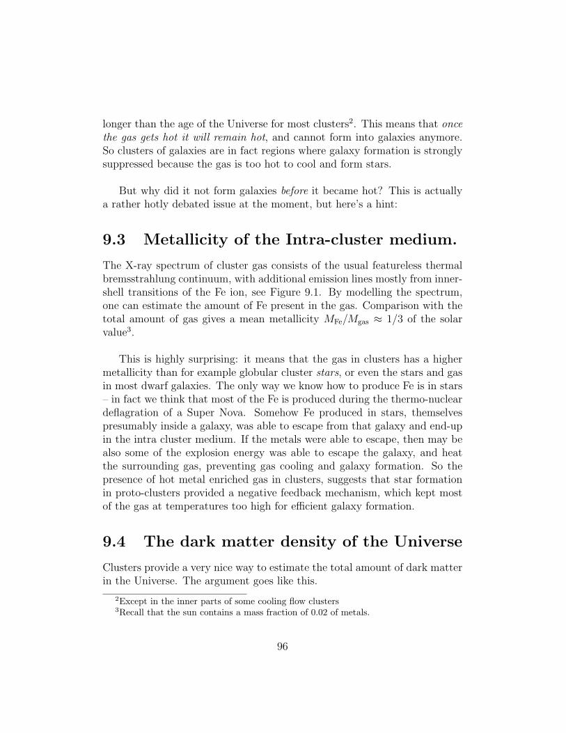
longer than the age of the Universe for most clusters2. This means that oncethe gas gets hot it will remain hot, and cannot form into galaxies anymore.So clusters of galaxies are in fact regions where galaxy formation is stronglysuppressed because the gas is too hot to cool and form stars.

But why did it not form galaxies before it became hot? This is actuallya rather hotly debated issue at the moment, but here’s a hint:

9.3 Metallicity of the Intra-cluster medium.

The X-ray spectrum of cluster gas consists of the usual featureless thermalbremsstrahlung continuum, with additional emission lines mostly from inner-shell transitions of the Fe ion, see Figure 9.1. By modelling the spectrum,one can estimate the amount of Fe present in the gas. Comparison with thetotal amount of gas gives a mean metallicity MFe/Mgas ≈ 1/3 of the solarvalue3.

This is highly surprising: it means that the gas in clusters has a highermetallicity than for example globular cluster stars, or even the stars and gasin most dwarf galaxies. The only way we know how to produce Fe is in stars– in fact we think that most of the Fe is produced during the thermo-nucleardeflagration of a Super Nova. Somehow Fe produced in stars, themselvespresumably inside a galaxy, was able to escape from that galaxy and end-upin the intra cluster medium. If the metals were able to escape, then may bealso some of the explosion energy was able to escape the galaxy, and heatthe surrounding gas, preventing gas cooling and galaxy formation. So thepresence of hot metal enriched gas in clusters, suggests that star formationin proto-clusters provided a negative feedback mechanism, which kept mostof the gas at temperatures too high for efficient galaxy formation.

9.4 The dark matter density of the Universe

Clusters provide a very nice way to estimate the total amount of dark matterin the Universe. The argument goes like this.

2Except in the inner parts of some cooling flow clusters3Recall that the sun contains a mass fraction of 0.02 of metals.

96

Figure 9.1: X-ray spectrum of the central region of the Centaurus cluster,taken by the ASCA X-ray satellite. It shows some emission lines and anabsorption edge (which are labelled) due to different components of the hotintra cluster medium.

97

Suppose the Universe starts-out smooth, with a (nearly) constant ratioω of dark matter to gas:

ω = ρdark matter/ρgas . (9.9)

As a cluster starts to form, the density of dark matter and of gas willincrease. But the potential well of the cluster is so deep, that it is probablya good approximation to assume that none of the dark matter, nor the gas,can ever escape the gravitational pull of the cluster. This means that theratio of the total dark matter to total gas mass in the cluster

Mcluster-in-dark-matterMcluster-in-gas

≈ ω . (9.10)

We could do slightly better by also including the mass in stars – but thatis a small correction anyway.

So we can find ω by determining Mcluster-in-dark-matter from dynamics,and Mcluster-in-gas from the X-ray emissivity. The result is ω ≈ 6.

Next we need an estimate of the mean baryonic density, ρgas. An ele-gant way is by determining the Deuterium abundance of gas4. Deuteriumis produced in the Big Bang and destroyed in stellar burning. So if we findDeuterium, we know it is left over from the Big Bang. Analysis of the spectraof quasars (we will discuss quasars soon) allows us to measure the Deuteriumabundance quite accurately. How does this help us? The missing link is thatthe gas density ρgas determines how much Deuterium is produced in the BigBang. Figure 9.2 shows how the abundance (with respect to hydrogen) ofelements produced in Big Bang nucleo-synthesis, as function of the baryondensity. The result is that the mean baryon density corresponds to of orderρgas/mp ≈ 2.2×10−7 hydrogen atoms per cm−3 (i.e. 3.75×10−31 g cm−3. Sothe density of paper/density of the screen you are reading this on, is about1030 times higher than the mean!

And so we’re done: the Deuterium abundance determines the gas densitythrough the known nuclear reactions that occurred during Big Bang nucleo-synthesis. And the dark matter density is ω ρgas with ω ∼ 6 determinedfrom clusters.

4Recall that the nucleus of a Deuterium atom differs from that of ordinary Hydrogenin that it has a proton and a neutron.

98

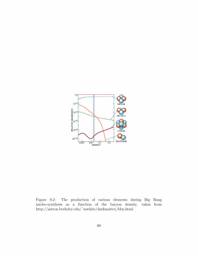
Figure 9.2: The production of various elements during Big Bangnucleo-synthesis as a function of the baryon density, taken fromhttp://astron.berkeley.edu/˜mwhite/darkmatter/bbn.html.

99

9.5 Summary

After having studied this lecture, you should be able to

• Define what is a cluster and a group of galaxies by listing some of theirproperties.

• Explain how galaxy motions suggest the presence of dark matter inclusters.

• Explain how X-ray observations suggest the presence of dark matter inclusters.

• Explain the origin of the high temperature of the cluster gas.

• Explain how we know that most of the baryons in a cluster are in hotgas, and not in stars.

• Explain why the high observed metallicity of the cluster gas suggeststhat some kind of stellar feedback mechanism prevented most of thegas turn into stars before it fell into the cluster.

• Explain how clusters have been used to estimate the mean dark matterdensity of the Universe.

100

Chapter 10

Galaxy statistics

Having studied some properties of spiral and elliptical galaxies in detail, wenow take a step back to examine the statistics of the different types. Thetwo degree-field galaxy redshift survey (2dF), and the Sloan Digital Sky sur-vey (SDSS), are two very recent galaxy redshift surveys. In a galaxy redshiftsurvey, one first identifies galaxies in images of the sky, and then takes aspectrum for each of them. Because the Universe is expanding, spectral linesof stars in a distant galaxy are shifted from the laboratory toward longerwavelengths: they are ‘redshifted’ . There is a relation between the distanceto the galaxy and its redshift, and so a galaxy redshift survey provides uswith the 3D position of a set of galaxies, about 2 × 105 for the 2dF, about106 for the SDSS. So what kind of general trends do they uncover? We willdiscuss some of these here.

The distribution of galaxies probably traces to some extent the distribu-tion of dark matter in the Universe. For example, we’ve seen that there isevidence for a lot of dark matter in the Universe as a whole (from the clus-ter argument), but also in individual galaxies, groups and clusters. And so,since we find that galaxies are distributed very inhomogeneous in groups andclusters, presumably also the dark matter is distributed in an inhomogeneousfashion. How? And what process determines this in the first place?

We have a good idea of how the dark matter is distributed on a cosmo-logical scale, from some general considerations, backed-up by observations ofthe micro-wave background (i.e. the sea of photons left-over from when theUniverse was still hot). Given this input, we can use numerical simulations

101

to predict how dark matter is clustered on large scales. The nice part ofthe story is that this theory is highly predictive, and does predict structuresin the galaxy distribution very similar to what we observe: a filamentarypattern delineating large regions of space devoid of galaxies, called ‘voids’ ,with regions of high galaxy density, clusters of galaxies, at the intersectionof the filaments.

10.1 The density-morphology relation

In the previous chapter we saw how some galaxies are in low density envi-ronments, some are in higher density groups, and others in dense clusterscontaining several hundred galaxies. Figure 10.1 shows that the fraction ofelliptical and S0 galaxies increases rapidly with increasing galaxy density. Inother words, in a region of high galaxy density, such as a dense group orcluster of galaxies, most galaxies tend to be S0 or E, and very few are oftype S. Vice versa, in regions of low galaxy density, most galaxies tend tobe of the type S. This is called the density-morphology relation, since itrelates the density of galaxies in a given region with their typicalmorphology (i.e. S, E, S0). Clearly this is telling us something on thenature of galaxy formation and evolution.

Recall from the movie I showed of the motion of galaxies in a cluster,that encounters between galaxies are very frequent in a region of high galaxydensity. Such tidal encounters could be responsible for converting S-typegalaxies into S0 and E, but other processes might operate as well. Recallthat we already discussed that this cannot be the whole story, since thestellar populations of Ss and Es tend to differ as well.

10.2 Galaxy scaling relations

10.2.1 The Tully-Fisher relation in spirals

The circular velocity as function of radius – the rotation curve – in spiralstends to be flat, i.e. the rotation velocity is independent of radius sufficientlyfar out in the disk. We argued in section 5.2 that this was evidence for thepresence of dark matter in spiral disks, since it implies lots of mass in the

102

Figure 10.1: The fraction of Elliptical (E), S0, and Spiral + Irregular (S+I)galaxies as function of the logarithm of the projected density, in galaxiesMpc−2. The data shown are for all cluster galaxies in the sample and forthe field. Also shown is an estimated scale of true space density in galaxiesMpc−3. The upper histogram show the number distribution of the galaxiesover the bins of projected density. Es and S0s tend to populated regions ofhigh galaxy density, and Ss regions of low galaxy density. From Dressler,ApJ 236, p. 351 (1980). 103

outer parts, whereas we see very little light there. Figure 10.2 compares themeasured rotation velocity Vc (written W in the figure) with the total abso-lute magnitude M = −2.5 log(L)+constant, for a sample of spiral galaxies.Brighter spirals (more negative M) rotate faster (larger W ). Since thefigure shows there to be a linear relation between M and Vc, it implies apower-law relation between the intrinsic luminosity L and the circular veloc-ity Vc, called the Tully-Fisher relation:

L ∝ V αc , α ≈ 4 . (10.1)

The slope α of this relation depends somewhat on which colour is used(i.e., does L refer to a V -band or I -band luminosity).

What is the origin of this relation? Remember1 that the circular velocityVc is determined by the enclosed mass M(< R),

V 2c =

GM(< R)

R. (10.2)

Let us introduce a global mass-to-light ratio, [M/L], as

[M/L] ≡ M(< R)

L, (10.3)

then

V 2c ∝ [M/L]

L

R. (10.4)

.The mass-to-light ratio [M/L] will depend on the type of stars in the

galaxy (which determines L), and the amount of dark matter (which mainlydeterminesM). The intensity I is the luminosity per unit area, I = L/(π R2),or solving for R

R ∼(L

I

)1/2

. (10.5)

Combining the last two equations gives

L ∝ V 4c

[M/L]2 I. (10.6)

1It is unfortunate that absolute magnitude and mass are both denoted by M .

104

Figure 10.2: R-band absolute magnitude M of spiral galaxies as functionof the maximum rotational velocity W = Vc (in km s−1). Brighter spiralgalaxies (more negative M ; recall that magnitude M is related to luminosityL as M = −2.5 log(L)+constant) rotate faster.

105

So the Tully-Fisher relation is reproduced, with α = 4, if the intensity Iand mass-to-light ratio [M/L] are independent of the luminosity of the galaxy.Notice that this is not a derivation of the Tully-Fisher relation: we are justtrying to understand what is required for spirals to follow this relation. Thefact that [M/L] and I are independent of L implies that somehow stars anddark matter are closely linked, or in other words: the star formation historyis largely determined by the mass of the dark halo of the galaxy.

10.2.2 The Faber-Jackson relation in ellipticals

The Faber-Jackson law, Figure 10.3, relates the velocity dispersion σ of thestars in an E-type galaxy with the total luminosity L,

L ∝ σ4 . (10.7)

Compare with the Tully-Fisher relation for spirals, Eq. (10.1): the veloc-ity dispersion σ takes the role of the circular velocity Vc.

Comparison of Figure 10.3 with Figure 10.2 shows that the scatter in theFaber-Jackson relation is quite a bit bigger than the scatter in the Tully-Fisher relation: at a given value of σ, there is a range of ±2 magnitudes inMB (i.e. a factor 2.5 in L), versus a few tenths of a magnitude for a givenvalue of Vc in the Tully-Fisher relation. So ellipticals follow a similar relationas spirals, with more luminous and hence more massive, ellipticals having alarge velocity dispersion, but the relation is not as tight as the correspondingVc(L) relation in spirals.

From all the parameters we can measure for an elliptical, the total lumi-nosity L, the velocity dispersion σ, the effective radius Re and the intensityIe (which both enter in the de Vaucouleurs profile, Eq. (3.2)), only threeare independent. So we can try to obtain a tighter relation by introducing asecond parameter in Eq. (10.7), for example Re. This is how it goes: supposethat the galaxy is in virial equilibrium, then its kinetic energy M σ2 will beproportional to its potential energy M2/Re, and so we expect

σ2 ∝ M

Re

. (10.8)

Introducing again the mass-to-light ratio, [M/L] this can be written as

106

Figure 10.3: B-band absolute magnitude M for a sample of elliptical galax-ies plotted versus the velocity dispersion σ (in km s−1). Brighter ellipticalsgalaxies (more negative MB; recall that magnitude M is related to luminosityL as M = −2.5 log(L)+constant) have a larger velocity dispersion.

107

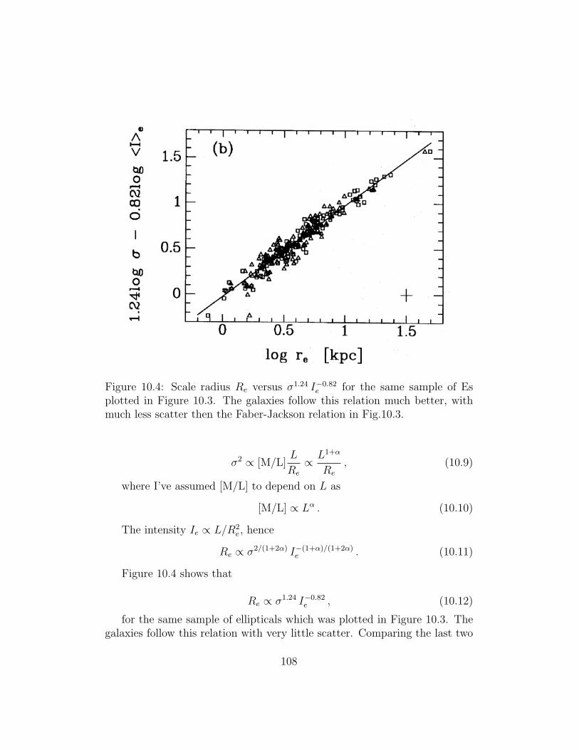
Figure 10.4: Scale radius Re versus σ1.24 I−0.82e for the same sample of Es

plotted in Figure 10.3. The galaxies follow this relation much better, withmuch less scatter then the Faber-Jackson relation in Fig.10.3.

σ2 ∝ [M/L]L

Re

∝ L1+α

Re

, (10.9)

where I’ve assumed [M/L] to depend on L as

[M/L] ∝ Lα . (10.10)

The intensity Ie ∝ L/R2e, hence

Re ∝ σ2/(1+2α) I−(1+α)/(1+2α)e . (10.11)

Figure 10.4 shows that

Re ∝ σ1.24 I−0.82e , (10.12)

for the same sample of ellipticals which was plotted in Figure 10.3. Thegalaxies follow this relation with very little scatter. Comparing the last two

108

equations shows that if we assume α ≈ 0.25, then Re ∝ σ1.33 I−0.82e – very

nearly the same as what the figure suggests. Put differently, if the mass-to-light ratio of ellipticals depends on luminosity as M/L ∝ L0.25, then wecan understand why ellipticals follow the relation plotted in Figure 10.4 sotightly.

The relation Eq. (10.12) is called the fundamental plane of ellipticalgalaxies. In four dimensional L, σ, Re and Ie space, galaxies do not occupythe whole space, but are restricted to a 3-dimensional surface defined byrelation (10.12), hence the name fundamental plane.

10.3 Tully-Fisher and Fundamental plane re-

lations as standard candles

The Tully-Fisher relation Eq. (10.1) relates the luminosity L of a galaxy to itscircular velocity. Now suppose we were able to measure the proportionalityconstant, by determining the luminosity for galaxies with known distance.Then by just measuring the circular velocity of a spiral galaxy, we couldinfer its luminosity hence absolute magnitude M , and consequently from itsapparent magnitude m obtain the distance r, since

m−M = 5 log(r)− 5 . (10.13)

Therefore, the Tully-Fisher relation can be used as a standard candle,since it allows us to determine the luminosity from the distance independentquantity Vc. Note also that Vc is relatively easy to determine from spectra,and so we have found a good way of measuring distances to distant galaxies!

The fundamental plane relation plotted in Figure 10.4 can also be usedas a standard candle: all we need to do is measure the velocity dispersion ofthe stars σ from a spectrum, and determine the intensity Ie (recall that thesurface brightness and hence also Ie is distance independent). By puttingthe E galaxy onto Figure 10.4, we then find Re. And so from the apparentsize of the galaxy, we can estimate its distance.

Both these methods are widely used, since measuring velocities is rela-tively easy from a good quality spectrum, and can be done even for faint

109

and/or distant galaxies. And since the scatter in the relations is small, wecan obtain a relatively accurate distance estimate.

10.4 Galaxy luminosity function

From a big galaxy redshift survey, we can make a histogram of the numberof galaxies with absolute luminosity between L and L+dL, where L is eitherthe total (or bolometric) luminosity, or the luminosity in some band, e.g.the B-band, per unit volume. Figure 10.5 shows that the number of faintgalaxies increases like a power law, whereas there is an abrupt cut-off towardthe brighter galaxies. This behaviour is well captured by the Schechterfunction

dN

dL/L?

= N?

(L

L?

)α

exp(−L/L?) . (10.14)

This function has three parameters, L?, α ∼ −1 and N?. For luminousgalaxies, it has an exponential cut-off for galaxies brighter than L?. For lessluminous galaxies, the number increases toward fainter galaxies, as Lα ∼ 1/L.Finally, N? is a normalisation constant, which determines the mean numberdensity of galaxies.

Values are N? ≈ 0.007Mpc−3, the steepness of the faint-end slope −1.3 ≤α ≤ −0.8, and the exponential cut-off sets in at L? ≈ 2 × 1010L in theB-band. From Table 3.1, we find that the total B-band luminosity of theMW is about 1.8 × 1010L, so the MW is just slightly fainter than an L?

galaxy.If the faint-end slope is steeper than α = −1, then the total number of

galaxies per unit volume, n =∫∞

0(dN/dL) dL diverges, because there are so

many faint galaxies. In reality, this does not happen of course, since theremust be some finite number of small galaxies. The mean luminosity densitycan be found from integrating

l =

∫ ∞

0

LdN

dLdL . (10.15)

This is the mean luminosity per unit volume. Combining this with themean density of the universe as obtained in section 9.4, we can estimate themass-to-light ratio for the Universe as a whole!

110

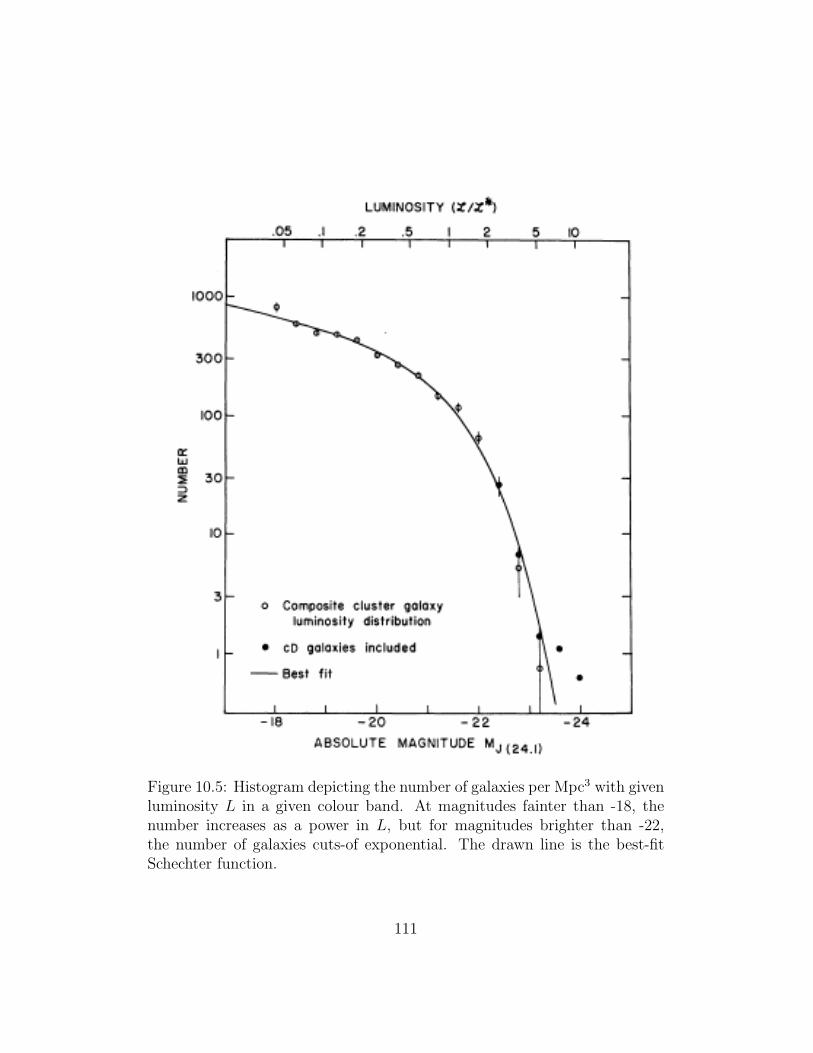
Figure 10.5: Histogram depicting the number of galaxies per Mpc3 with givenluminosity L in a given colour band. At magnitudes fainter than -18, thenumber increases as a power in L, but for magnitudes brighter than -22,the number of galaxies cuts-of exponential. The drawn line is the best-fitSchechter function.

111

Finally, Figure 10.6 shows how the Schechter luminosity function is com-posed of contributions from the various galaxy types, E, S0 and the differenttypes of spirals, and irregular galaxies. Top panel is for a sample of galaxiesaway from big clusters, bottom panel refers to the Virgo cluster. Here werecognise the density-morphology once more: most of the brighter galaxiesin the top panel are Spirals, whereas in the cluster sample, E an S0s play amuch bigger role.

10.5 Epilogue

The classification of galaxies that we have used so far, in terms of spirals andellipticals, is based largely on how these galaxies appear in pictures. Withseveral 105 galaxies in modern surveys, it is not really possible to eye-ballall of them in order to classify them. In addition, it is not even neces-sarily the best way, and certainly not the only way, of classifying galaxiesand identifying different types. With so many spectra and images available,new statistical techniques are presently being developed, where computerprograms which do not suffer from human prejudices, such as principle com-ponent analysis and neural networks, decide how galaxies should be groupedand classified.

112

Figure 10.6: This plot shows how the galaxy luminosity function for galaxiesin a cluster (bottom panel is for the Virgo cluster) or galaxies not in a cluster(‘field galaxies’, top panel), is made-up from the mix of galaxy types.

113

10.6 Summary

After having studied this lecture, you should be able to

• describe the density-morphology relation for galaxies

• explain what is the Tully-Fisher relation, and derive what it implies forthe mass-to-light ratio and surface brightness of spirals

• explain the Faber-Jackson and Fundamental Plane relations for Ellip-ticals, and derive what the fundamental plane relation implies for themass-to-light ratio of ellipticals

• explain how Tully-Fisher and Fundamental Plane relations are used asstandard candles.

• explain what is the luminosity function of galaxies and sketch it.

114

Chapter 11

Active Galactic Nuclei

Some galaxies harbour immensely powerful sources of radiation in their cen-tres, detected from the longest (radio) to the shortest wavelengths (X-rays):these are called Active Galactic Nuclei (or AGN for short). We think they arepowered by the accretion of matter onto super massive black holes (SMBH),the same process that powers some galactic X-ray binaries. However, theSMBH have masses ranging from 106 to 109M, and so, unlike galactic blackholes, cannot be stellar remnants. We think that most or even all reason-ably massive galaxies have a SMBH lurking in their centres, but only a smallfraction of these are ‘active’ at any given time. The evidence that the MWhas its own SMBH is particularly impressive.

Where do these SMBHs come from? Are they really black holes (i.e. ob-jects with an event horizon) or are they just very massive, extremely denseobjects (MDO)? Why are some associated with strong radio-sources (radio-loud AGN), but others are not? How do radio-loud AGN power the immenseradio-lobes we observe? What is the effect of the AGN on the galaxy itself?Most of these questions remain without a clear answer, even today.

I will start by discussing some of the observations of AGN. Then I’ll takeyou through the evidence that these really are black holes, but leave it upto you to decide whether you believe it or not. My own view is that theevidence for super massive and very dense objects is very convincing – but Ihave not seen evidence for an event horizon (yet).

115

11.1 Discovery and observational properties

Carl Seyfert reported in 1943 that a small fraction of galaxies have a verybright nucleus, which is a source of broad emission lines produced by atomsin a wide range of ionisation stages. These nuclei appear unresolved, i.e.they are stellar in appearance.

After World War II, radio surveys discovered a very bright radio source,called Cygnus A. Given the accurate radio-position of the source, the opticalcounterpart was identified with a peculiar-looking cD-galaxy, whose centre isencircled by a ring of dust.

The spectral lines in the optical spectrum of Cygnus A are redshifted to∆λ/λlaboratory = 0.057. In terms of a Doppler shift, this corresponds to arecession velocity of 16000km s−1. From this, one can estimate the distanceto Cygnus A1, d ∼ 240Mpc, and hence compute the implied luminosity ofthe radio source, which turned out to be roughly ten times the total energyoutput (i.e. over all wavelengths) of the MW.

In 1960, Thomas Matthews and Alan Sandage were trying to find the op-tical counterpart of another bright radio-source, called 3C 482. They founda 16th magnitude star like object, with a very curious spectrum, displayingbroad emission lines that they could not identify with any known element ormolecule. Sandage put it very scientifically: ‘This thing is exceedingly weird’.In 1963, another such weird object, 3C 273 turned-up. Given they lookedlike stars, in that they were point like (unlike galaxies which are extended),they were called quasi-stellar objects, or QSOs.

In the same year, the Dutch astronomer Maarten Schmidt recognised thatthe pattern of lines in 3C 273 was similar to the Balmer series3 of the Hy-drogen atom – but only if they were redshifted to the (improbably large ?)value of ∆λ/λ = 0.16, implying a recession velocity of 0.16c and a distanceof 630Mpc. The distance to 3C 48 was even greater: a recession velocity of

1The redshifting of the spectral lines is due to the expansion of the Universe. By mea-suring the expansion rate, one can convert redshift to distance, assuming a cosmologicalmodel.

2The C stands for Cambridge – this is the third Cambridge radio-survey.3The Balmer series is the series of electronic transitions in an atom which starts with

the Hα line (n = 3 → n = 2), then Hβ (n = 4 → n = 2) etc.

116

0.367c and a distance4 of 1800Mpc.

For a distance of d = 630Mpc to 3C 273, the distance modulus m−M =5 log(d/10) ≈ 39. The apparent magnitude of 3C 273 is m = 12.8 (in theV-band), hence the absolute magnitude is M = −26. Since the Sun’s abso-lute magnitude M = +5.-ish, it implies that 3C 273 is 100.4×31 ∼ 1012 timesbrighter than the Sun, or 100 times as bright as the entire MW. Give or takea factor of a few. What kind of object can be so small yet so tremendouslypowerful?

Since then, many more QSOs have been discovered, we know severalhundred thousands of them by now. The current5 record holder has ∆λ/λ =6.3. In terms of recession velocity, this is 6 times the speed of light (!),showing that interpreting such a redshift in terms of Doppler shift is not agood idea6. The luminosity of the brighter QSOs can range up to 105 timesthe luminosity of the MW.

The shear luminosity of QSOs alone already suggests we are looking atsomething unusual. In addition, some of these QSOs have radio-lobes whichare tens of times the size of a galaxy. What is the engine that powers them?

11.2 The central engine, and unification schemes

QSOs certainly are very bright. But are they unusually bright? Yes. Theargument is neat, and based on the variability of QSOs. The luminosity ofQSOs varies on a range of time-scales – hours, days, and months, dependingon the wavelength at which you observe them. But variations in the X-rayproperties tend to have very short time-scales, of order of minutes. Now thisimplies that the X-rays come from a small region – of the order of light min-utes. To come to this conclusion, all we need is to say that the information

4The ‘velocity’ of such distant objects is not a real velocity in the sense that somethingis moving. The velocity results from space expanding, and it is often better to not convertthis to velocity at all – just use the cosmological model to find the relation between theredshift z = ∆λ/λ and distance.

5March 2003. The text book we’re using, OC, states we know 5000 of them. And thatwe know ‘several’ with redshift greater than 4. This just shows you how rapidly this fieldis evolving.

6You may argue we should use special relativity. In fact, we need general relativity tomake proper sense of this.

117

about the variation has to be able to travel across the object that is produc-ing the emission, and the fastest the information can travel is the speed oflight, c. Hence the engine is small, of the order of light minutes. Recall thatthe distance to the Sun is 8 light minutes7. And so we need to find a smallengine, size of order a solar system, that can produce as much energy as allthe stars in 100 galaxies combined.

The most efficient way we know of for producing energy is by mass ac-cretion onto a compact object8. Recall from the stellar part of this course,that stellar X-ray binaries produce their energies this way. The estimatedefficiency (in terms of the rest mass energy mc2 of the fuel converted intoradiation) is 10 per cent, which you can compare to the second most efficientway, nuclear fusion, at 0.7 per cent.

Recall also from those lectures that there is a maximum luminosity – theEddington luminosity – that a spherical object in equilibrium can produce. Ifthe luminosity is higher, than the radiation pressure becomes larger than thegravitational force, and the object can no longer remain bound. Comparingthe Eddington luminosity with the QSO’s luminosity, gives us a lower limitto the masses involved, of order 108M. Given such a small size, and sucha large mass, Donald Lynden-Bell and Martin Rees suggested that accretiononto a massive black hole must be the energy source powering QSOs.

There is a problem though. A black hole is characterised by just twonumbers: its mass, and its spin (i.e. its rotational energy). But there isa wide variety of QSOs out there. For example, some have jets, and strongradio sources, others don’t. The time variability is by no means regular. Howcan that be, if there is only two parameters that characterise the engine?

The gas is thought to accrete onto the SMBH by passing through anaccretion disk, where it has to loose enough angular momentum to be ableto accrete. This introduces a third parameter: the orientation of the diskwith respect to the observer. The most popular unification schemes9 suggest

7To do this properly, we need to take (special) relativistic effects into account. But ifyou do everything properly, you get a similar answer to what we found.

8Actually, annihilation of matter–anti-matter is even better!9i.e. theories that try to explain QSO activity in terms of a single model – accretion

onto a SMBH.

118

that orientation effects determine many of the observed properties of theQSO. But there is by no means a simple answer to understand the widevariety of properties.

11.3 Evidence for a SMBH

I10 am going to take you through several lines of evidence that QSOs areindeed powered by a SMBH. You may think that the fact that we needan engine the size of the solar system that produces as much energy as 100galaxies together, would seem enough of a proof on its own. So let me discussjust one alternative: suppose there is a dense cluster of stars in the centreof a galaxy hosting a QSO, and what we are seeing is the combined effect ofseveral tens of SNe explosions. A single SN at its peak luminosity is aboutas bright as a whole galaxy, so we need about 100 SNe and we’re done. Isthis a reasonable model for AGN?

The model has withstood for several decades, but it does have somepitfalls. For example, we don’t know how such SNe would generate thetremendous radio-lobes that some QSOs have. But then, we don’t knowhow a SMBH does that either. As Luis Ho puts it: ‘our confidence thatSMBHs must power AGN largely rests on the implausibility of alternativeexplanations’. Most of the arguments in the next sections just suggest thepresence of a very massive, dense object (MDO) in the centre of galaxies (notjust in galaxies harbouring a QSO – in fact, some of the best evidence is ingalaxies which do not have an active QSO), but not really require the MDOto be a black hole, i.e. an object with an event horizon.

11.3.1 Photometry

The density of stars near a MDO will rise very sharply in the region wherethe MDO dominates the mass. This basically comes from Jeans’ equationsexpressing hydrostatic equilibrium, in the form

GMDO

r2= −∇ρσ

2

ρ. (11.1)

10I will follow a nice review paper by Luis Ho, seehttp://nedwww.ipac.caltech.edu/level5/March01/Ho/Ho.html for the full text.

119

If the velocity dispersion does not rise very rapidly, σ2 ≈ constant, thenthe density must rise very rapidly, d ln(ρ)/dr ∝ −1/r2 hence ρ ∝ exp(1/r).So a rapid increase in density of light toward the centre could signify thepresence of a SMBH.

However, the region where the MDO dominates may be very small, of or-der rMDO ≈ GMDO/σ

2. As viewed from Earth for a QSO at distance D, theangular extent will be≈ 1arcsec(MDO/2×108M) (σ/200km s−1)−2 (D/5Mpc).Such a small extent is hard to see from the ground (due to atmospheric see-ing), and Hubble Space Telescope (HST) will be needed.

Now some galaxies do indeed show a dramatic increase in brightness – acusp – toward the centre, even at HST resolution. Unfortunately, it is alsoknown that the velocity dispersion σ2 is not constant. So we cannot claimthis proves the presence of a MDO – it’s a good indication though.

11.3.2 Stellar kinematics

The previous method was not perfect, since we did not take into account thatσ may vary. Now close enough to the MDO where it dominates the mass, weshould be able to detect the Keplerian rise in velocity dispersion σ ∝ r−1/2.So people tried to determine σ(r) close to the centre.

However again there is a loop hole: σ(r) can grow as well in case thevelocity distribution becomes anisotropic, e.g. in spherical coordinates σ2

r 6=σ2

θ 6= σ2φ. Again using the Jeans’ equations, the radial variation in mass can

be related to the stellar velocity dispersion as11

M(< r) =V 2 r

G+σ2

r r

G

×[−d ln νσ2

r

dr+ (

σ2θ + σ2

φ

σ2r

− 2)

]. (11.2)

V is the circular velocity. Clearly, if we were allowed to choose the threecomponents of σ2, we could balance a large increase in density with thevelocity tensor becoming more anisotropic, even in the absence of a MDO.

Observed galaxies do indeed show a large increase in σ close to the centre,but we cannot rule out that this is due to anisotropic velocities, and not tothe presence of a MDO. So once more, the evidence is a bit circumstantial.

11I just state the result and don’t expect you to derive it.

120

11.3.3 Stellar kinematics in the MW centre

The MW centre has a weak AGN in its centre, identified with the radiosource Sagittarius A.

Over the past couple of years, Genzel and collaborators measured thekinematics of stars close to the MW centre from near-IR spectra12 Theyalso determined very accurate positions of the stars. By doing this overseveral consecutive years, they were able to measure not just the 3D propermotions of the stars, but also measure accelerations. In fact they were ableto follow one star over nearly a whole orbit, when it swung passed the centreat velocities approaching 1000km s−1.

So first of all, they demonstrated that there is indeed a very massive‘dark’ object in the centre of the MW. Using Kepler’s laws, they were ableto put very stringent limits on the mass of the central concentration, MDO ≈2.6 × 106M, in a region smaller than 0.006pc, implying an enormous massdensity higher than 2 × 1012M/pc3. This leaves almost no room to escapethe conclusion that the MDO is indeed a SMBH, at least in the MW.

The presence of the large mass is also supported by the presence of othervery high velocity stars. From that, and from the fact that the putativecentre, i.e. the radio source Sagittarius A itself does not seem to move,Genzel derived a lower limit to the density of 3× 1020M/pc3.

Incidentally, they also showed that the velocity dispersion remains nearlyisotropic, and so unless the MW is peculiar, this then strengthens the casefor SMBHs in other galaxies, from the arguments in the previous section.

11.3.4 Methods based on gas kinematics

Unlike the situation for stars where anisotropy clouds the interpretation, gaskinematics is much easier to interpret if the gas is in Keplerian motion13.There are two caveats, however. There may be non-gravitational forces act-ing on the gas, magnetic fields for example. Second, there is no a priorireason for the gas to be in Keplerian motion. So we need to lucky then.

12Recall the need to go to the IR: there is a lot of absorption by dust toward the MWcentre but IR-light undergoes far less absorption.

13Whereas stars can freely move through one another, gas motion must be ordered notto produce shocks.

121

Optical emission lines Several examples of nuclear disks around centresof galaxies were found by HST. For example for M87 (the big elliptical in theVirgo cluster), HST measurements found a Keplerian rotation curve in thedisk with a velocity of 1000km s−1 at a distance of 19pc from the centre14.This implies a MDO with mass ≈ 2.4× 109M. Similar evidence for a MDOnow exists for other galaxies as well.

Maser emission Some AGN have luminous maser15 sources close to thecentre. Radio observations of these maser lines show that the masers are innearly Keplerian rotation, and from the speed one can place tight constraintson the mass density of the MDO, > 5× 1012M.

Reverberation mapping Another elegant way to determine the extentof an AGN is ‘reverberation mapping’. Many of the emission lines seen froman AGN are due to the light from the central source being reprocessed by thesurrounding material. As the central source varies in luminosity, the emissionlines vary as well, but with a time-lag that corresponds to the light-traveltime between the central source and the line-emitting gas. So by measuringthe time-lag, we can estimate the size of the light-emitting region.

11.3.5 Profile of X-ray lines

The Fe Kα line at 6.4keV is a common feature in the X-ray spectra of AGN. Itis thought to arise from fluorescence of the X-ray continuum off cold materialin the surroundings, possible associated with the accretion disk around theSMBH.

This line is produced very close to the SMBH, and it exhibits Dopplermotions approaching relativistic speeds, ∼ 105km s−1 ≈ 0.3c. Now crucially,the line-profile displays asymmetries consistent with a gravitational redshift.The photons lose energy as they climb out of the deep potential well near theblack hole. In doing so, their wavelengths become longer – a ‘gravitationalredshift’.

For the AGN galaxy MCG-6-30-15, the best fitting accretion disk has aninner radius of 6 Schwarzschild radii, i.e. very close to the event horizon. A

14Don’t get confused with evidence for dark matter from flat rotation curves. Herewe are looking close to the centre, whereas for rotation curves we were looking at largedistances, ∼ 20kpc from the centre.

15A maser is a laser that operates in the mm regime.

122

similar analysis has now been performed for other AGN as well. The shapeof the line probably provides the best evidence to date for theexistence of a SMBH. However, other mechanisms for generating the lineprofile are possible, but implausible. With better data, detailed modelling ofthe profile even has the potential to determine the spin of the SMBH.

11.4 Discussion

So are you convinced of the existence of SMBH? I think the evidence fromstellar motions around the MW centre is truly impressive. The Fe Kα linecomes very close to convincing me as well. But I think we really need tosee relativistic motions or phenomena originating close to the Schwardschildradius to clinch the matter.

So let me summarise. We have evidence that probably most, if not all,galaxies with masses of order the MW mass or higher, have a SMBH in theircentres. It also transpires that the mass of the SMBH seems to correlatewith the mass of the galaxy: the more massive the galaxy, the more massivethe SMBH. What does that tell us about the formation of the galaxy or ofthe SMBH? We don’t know (yet!).

Also, if most galaxies contain a SMBH, then why are there so manytimes fewer QSOs than galaxies? Indeed, QSOs are rare, so only a verysmall fraction of SMBH is active and produces AGN activity at any onetime. The best guess is that there is no gas accreting onto those SMBHs:these inactive QSOs are starved for food. Still it may be a bit surprising thatso many black holes are so very black – some gas is lost by the stars closeto the centre, which somehow must be accreted onto the black hole withoutproducing much radiation.

And finally: if a star ventures too close to a SMBH, then it may be tornapart as a result of the tidal forces from the SMBH. This could lead to avery bright flare, which would last for of order months. The realisation thatSMBHs may be quite common provides fresh motivation to search for suchflares. Upcoming missions designed to detect SNe will find these flares – ifthey exist.

123

11.5 Summary

After having studied this lecture, you should be able to

• describe observational properties of AGN.

• describe briefly the current paradigm for energy generation in AGN(mass accretion through a disk onto a SMBH)

• describe three arguments that suggest the presence of SMBHs in galax-ies.

124

Chapter 12

Gravitational lensing

According to the theory of General Relativity, a massive object distorts thespace around it. For example, the distortion in space due to the the Sunmakes the planets go around it. When light travels through such a distortedspace, it also gets deflected.

Therefore, in general, the gravitational field generated by a mass distri-bution will distort the images you see of background sources, pretty muchlike the hot air above a road distorts the view behind it. This is in fact agood way to think about this phenomena: it is as if space has an index ofrefraction which varies in space, because the gravitational field also varies inspace. (Whereas it is of course the varying temperature that causes the re-fractive index to vary above the hot road.) This effect is called ‘gravitationallensing’, although ‘gravitational miraging’ might be a better description sincethe distortion is more ‘blurring’ (like the hot air) than focusing (like a properlens).

A very good introduction to the subject is the recent review by JoachimWambsganss1. Scientists are not very good at reconstructing the history of asubject, but Joachim claims that a German physicist in 1804 was the first tosuggest that gravitational lensing might be observable, for example in termsof the deflection of star light passing close to the Sun.

There are several possible observable effects of gravitational lensing: (1)

1see http://www.livingreviews.org/Articles/Volume1/1998-12wamb

125

deflection: the image position is displaced from the source position, (2) am-plification: the image may be become brighter or fainter, (3) distortion: if thesource is extended (for example lensing of a galaxy by a galaxy cluster), thenlensing may distort the image, (4) multiple images: in general a single sourcewill be imaged in multiple images. All these effects have been observed.

In general, the deflection and amplification in real systems is usually verysmall, therefore our view of the Universe is not greatly distorted by gravita-tional lensing. But occasionally, some objects are lensed quite strongly. We’llstart by deriving a very simple – but unfortunately not quite correct – ex-pression for the deflection angle, but also state the correct result. Then we’llbe armed with enough understanding to look at some applications of lensing,and you’ll realise the tremendous potential of this technique, on a really widevariety of fronts, from constraining the nature of dark matter, via measuringthe masses of galaxy clusters, to detecting planets and constraining modelsof stars.

12.1 The lens equation

12.1.1 Bending of light

Suppose a particle with mass m and velocity v flies with impact parameter bpast an object with mass M . The gravitational pull of M will deflect m, andgive it a component v⊥ perpendicular to its initial v. For the case m = M ,this is in fact the situation we envisaged when deriving the relaxation timein Section 8.1. There we found that (see Eq. 8.3) when the deflection angleα is small,

v⊥ =2GM

b v. (12.1)

Convince yourself that this is the correct result also in case m 6= M .Finally, since tan(α) = v⊥/v and when α is small so that tan(α) ≈ α,

α =2GM

b v2. (12.2)

Now here’s the trick: the expression for α does not depend on the massm of the particle being reflected, only on the mass M of the deflector. So wemight be tempted to put m = 0, v = c and claim this is the angle by which

126

light will be deflected as well.

Applying this to starlight passing close to the sun, hence using M = M,R = R = 7 × 105km, we get α = 0.83arcsec – so α 1 is certainly satis-fied. This was actually the value Einstein found in 1911, though one JohannSoldner already obtained it almost a century earlier.

Curiously, the answer is wrong! Once Einstein formulated his theory ofGeneral Relativity, he did the problem again, and found that the deflectionangle is twice our ‘Newtonian’ value. So the correct deflection angle for lightis

α =4GM

b c2. (12.3)

and it was of course a great vindication of the theory when Eddingtonverified this during a solar eclipse in 1920. Note that the deflection angleincreases with M and decreases with b – the closer you pass to the moremassive an object, the bigger is the deflection.

In the case of the Sun, the deflection is so small that you might thinkit is of little use in Astronomy. This was actually true for a long time, butrecently it has really taken off as a new way of looking at the Universe. BeforeI show you some applications, we need to do a little bit more maths first.

12.1.2 Point-like lens and source

Suppose the light source (S), lensing mass M (L) and observer (O) are ex-actly aligned, as in Fig.12.1. Also assume they are all point like (i.e. notextended like for example a galaxy). Light rays from S are deflected by Lover an angle α toward O. Because of symmetry of the situation, O sees aring of light around L: an Einstein ring. Of course the figure is not to scale:α should be small if we want to apply the lensing equation.

Introducing the distances between observer and lens DOL, observer andsource DOS, and lens and source DLS, we can compute RE and the angle θE

under which O sees the ring. Since ψ + θE = α we get, using the lensingequation and the figure,

127

Figure 12.1: The source (S), lens (L) and observer (O) are all aligned. Lightfrom S is deflected by an angle α toward O. Because of symmetry, O sees thesource S as ring of radius RE centred around L.

128

Figure 12.2: The source (S), lens (L) and observer (O) are now misaligned,and O sees two images of S, one of which is depicted here while the otherone lies on the other side of L.

129

θE =RE

DOL

ψ =RE

DSL

α =4GM

RE c2, (12.4)

and hence

R2E =

4GM

c2DOL(DOS −DOL)

DOS

. (12.5)

If O, L and S are not aligned, as in Fig.12.2, then O does not see aring. Denote the angular position of S from the line OL by θS, and theangle between S and its image I by θI . Then from the figure you see thatα(DOS − DOL) = DOS(θI − θS). A bit of juggling and using the lensingequation gets you to:

θ2I − θIθS = θ2

E . (12.6)

This is a quadratic equation for θI for a given θS and so there will be twoimages, at positions θI,±.

Often, the change in position will be very small and not observable. Butbesides being lensed, an image will also be magnified (or de-magnified). Sowhen the displacement is too small to see two images, you’ll only see onebut magnified by total magnification A = A+ +A− of each image separately.Interestingly, for a small fraction of peculiar alignments, A may diverge, andso potentially you can get very large amplifications.

12.1.3 More realistic lensing

In the previous section we assumed that both lens and source where just pointmasses. When the lens is extended, you can get multiple images (3,5,7,...),depending on the impact parameter and the mass distribution of the lens.If the source is extended as well, then different parts of the source may bedeflected and amplified in various ways, and so the image may be highlydeformed. We are now in a position to look for applications. To wet yourappetite, let me show you two beautiful examples.

130

Figure 12.3 shows an Einstein ring. The lens is probably an ellipticalgalaxy, and the source a more distant spiral. Because of the near perfectalignment, the spiral has been imaged into a ring.

Figure 12.4 shows how a nearby spiral galaxy has lensed a very distantbackground quasar and produced multiple images of it, in this case five.

12.2 Micro-lensing

If2 both source and lens are stars, then we can use our results from thepoint-like models. We expect very small deflections, but potentially largemagnifications. We only get large magnifications for chance alignments.

So as foreground stars move in front of background stars – for examplea star in the Milky Way disk moves in front of a star in the bulge – it canoccasionally amplify the bulge star by a large amount. However, since thealignment has to be very precise to get a large amplification, the bulge starwill not be amplified for a long time, before the disk star moves away fromthe ideal lensing alignment.

Because the alignment has to be so good, you need to look at millions ofstars to have a chance of seeing significant amplification. So people observedmillions of stars toward the LMC and toward the bulge, to find stars thatbrightened by a lot over a few days. This phenomena is called micro-lensing(because the deflection angle is so small, ∼ 10−6arcsec).

There is one crucial aspect of lensing that we haven’t paid attention toyet: the deflection and amplification is independent of the wavelength of thelight, as you can see from Eq. (12.3). This is important if you want todetect micro-lensing, because the brightness of many stars varies anyway,because they are variable stars. But in general, the change in brightness fora variable star depends on the colour you observe it in. But the change inbrightness due to micro-lensing is colour independent. This makes it possibleto distinguish variable stars from lensed stars. In addition, the light curve –luminosity as function of time – is very easily computed in terms of M andthe relative velocity of L and S. Combined, it allows one to confidently detectmicro-lensing, and distinguish it from the case where the star is intrinsicallyvarying. Figure 12.5 shows an example of micro-lensing of a star in the LMC,

2I took this part, including the figures, from W Evans’ 2003 review, see astro-ph/0304252

131

Figure 12.3: Hubble Space Telescope image of an Einstein ring, where afortuitous alignment has caused an intervening elliptical galaxy (the centralspot) to lens a background spiral galaxy into a ring.

132

Figure 12.4: Hubble Space Telescope image of the ‘Einstein cross’, where adistant quasar has been lensed into multiple images by an intervening spiralgalaxy.

133

Figure 12.5: Luminosity of a star in the LMC in the blue (top) and red(bottom) as a function of time. Lensing causes it to brighten around day420.

134

which brightens considerably around day 420, equally much in the blue as inthe red.

Although we so far only considered lensing by stars, in fact any massiveobject will produce lensing. This has been exploited by the MACHO col-laboration3 to constrain the nature of the dark matter in the halo of theMilky Way. Indeed, suppose dark matter consisted of some type of massiveobjects, like black holes, or Jupiter-like objects, or some type of MAssiveCompact Halo Object in general. Since we know that the outer parts of theMilky Way halo is dominated by dark matter, there should be many suchobjects between the Sun and the LMC. If they exist, then we can detectthem by their lensing signal.

To detect such MACHO’s, the collaboration imaged millions of stars inthe LMC for four years, and indeed found several lensing events like the onepictured in Fig.12.5. However, it is now believed that in each case, the lensis actually a normal star in the LMC, and not some exotic kind of matter.As a consequence, this experiment has now ruled-out a wide range of darkmatter candidates. If the dark matter is some type of elementary particle,it will not lens LMC stars (well, it will, butM → 0!), so that is still an option.

The future of micro-lensing is very bright. Suppose for example that thelens is a binary star – then the light curve of the lensed object may be muchmore complicated, as the source may be lensed by each component of thebinary in turn. Such events have already been detected toward the bulge.This is also a very promising way for detecting planets around distant stars,and planned satellite missions will undoubtedly detect planets in this way.

12.3 Strong lensing

The effect of lensing increases with the mass of the lens. So can we usegalaxy clusters with masses ∼ 1015M as lens? Yes we can, and we do getlarge deflections of several tens of arc seconds up to several arc minutes.

Figure 12.6 is an HST picture of a rich cluster of galaxies – you can seemany massive elliptical galaxies in the cluster, as you’d expect. Because of

3http://wwwmacho.mcmaster.ca/

135

Figure 12.6: Hubble Space Telescope image of the rich cluster of galaxiesAbell 2218. The large galaxies in the image are all massive elliptical galaxiesin this galaxy cluster. Tens of radial arcs are images of background galaxiesthat have been lensed and distorted by the dark matter in the cluster.136

the superb image quality of HST, you also see tens of radial arcs, centredon the cluster centre. These are images of galaxies that lie far behind thecluster, that have been lensed by the dark matter in the cluster. Clearly,their images have been distorted a lot by the lensing process.

Several of these lensed galaxies have multiple images, i.e. you see thesame galaxy at various positions in the cluster. In addition, some images ofgalaxies may have been magnified by a lot, sometimes as much as a factorof 30. Because of this, the cluster really acts as a telescope, allowing youto study faint and distant galaxies, using the dark matter in the cluster toincrease the brightness of the galaxy light. Astronomers are now deliberatelytargeting foreground clusters in order to study better the faint galaxies be-hind it, that would not be bright enough to observe in the absence of lensing.

The positions and magnifications of these lensed galaxies can also be usedto infer the distribution of matter in the cluster, since it is that which causesthe lensing. This is a very important application of lensing. Recall howwe inferred the presence of dark matter in clusters so far. Assuming virialequilibrium, we estimated the mass in the cluster from the velocities of thegalaxies. Another way was to assume that the hot gas in the cluster was inhydrostatic equilibrium, and obtain the mass from the X-ray observations ofthe hot gas. In either case, the computed masses were far higher than whatwe could account for in either stars or gas – hence our claim that galaxyclusters contained a lot of dark matter.

But we had to assume something – virial equilibrium for the galaxies, hy-drostatic equilibrium for the gas. The great thing about gravitational lensingis that all we care about is the amount of mass present: we do not need toassume any type of equilibrium, since the velocity of the mass is irrelevant.The lensing mass and X-ray masses are in reasonably good agreement for thestill relatively few clusters studied so far, and so this is again very convincingevidence for the presence of dark matter.

137

12.4 Weak lensing

The arc lets seen in clusters arise because the image of the background galaxyis strongly deformed. Equation (12.3) shows that as we look at galaxiesfurther from the projected centre of the cluster – and hence as the impactparameter b increases – the distortion will become smaller and smaller. Even-tually, we won’t be able to detect the deformation for a single galaxy anymore, but we could look at many galaxies in a given small patch of sky,and try to determine whether perhaps they are all slightly elongated in thesame direction, as would be the case if there were a lot of mass nearby. Thisis called weak lensing: you try to identify the presence of a large mass ina given direction, from the fact that galaxies nearby in projection, tend tobe elongated in a same direction. Astronomers are now searching throughstacks of images trying to find whether may be there are some really massiveobjects that have no galaxies associated with them. Another use of weaklensing is just try to map directly the distribution of matter in the Universe,irrespective of whether it emits light as well.

138

12.5 Summary

After having studied this lecture, you should be able to

• derive the Newtonian lensing equation (12.2)

• explain why alignment produces an Einstein ring, and derive its radius.

• explain how micro-lensing works and has been used to search for mas-sive compact halo objects in the Milky Way halo

• explain how gravitational lensing has been used to estimate the massof galaxy clusters, and hence infer that they contain dark matter.

139

Contents

1 Introduction 41.1 Historical perspective . . . . . . . . . . . . . . . . . . . . . . . 41.2 Bringing order to the zoo of galaxies . . . . . . . . . . . . . . 5

1.2.1 Vocabulary . . . . . . . . . . . . . . . . . . . . . . . . 51.2.2 Galaxy properties . . . . . . . . . . . . . . . . . . . . . 7

1.3 Summary . . . . . . . . . . . . . . . . . . . . . . . . . . . . . 12

2 The discovery of the Milky Way and of other galaxies 132.1 The main observables . . . . . . . . . . . . . . . . . . . . . . . 132.2 The main players, their measurements, and their mistakes . . 16

2.2.1 Time-line . . . . . . . . . . . . . . . . . . . . . . . . . 182.3 Absorption, scattering and reddening . . . . . . . . . . . . . . 202.4 Summary . . . . . . . . . . . . . . . . . . . . . . . . . . . . . 22

3 The modern view of the Milky Way 233.1 New technologies . . . . . . . . . . . . . . . . . . . . . . . . . 23

3.1.1 Radio-astronomy . . . . . . . . . . . . . . . . . . . . . 233.1.2 Infrared observations . . . . . . . . . . . . . . . . . . . 243.1.3 Star-counts, again . . . . . . . . . . . . . . . . . . . . . 25

3.2 The components of the Milky Way . . . . . . . . . . . . . . . 253.2.1 The disk . . . . . . . . . . . . . . . . . . . . . . . . . . 263.2.2 The thick disk . . . . . . . . . . . . . . . . . . . . . . . 273.2.3 The bulge . . . . . . . . . . . . . . . . . . . . . . . . . 273.2.4 The stellar halo . . . . . . . . . . . . . . . . . . . . . . 283.2.5 The dark matter halo . . . . . . . . . . . . . . . . . . . 29

3.3 Metallicity of stars . . . . . . . . . . . . . . . . . . . . . . . . 293.3.1 Galactic Coordinates . . . . . . . . . . . . . . . . . . . 30

3.4 Summary . . . . . . . . . . . . . . . . . . . . . . . . . . . . . 33

140

4 The Interstellar Medium 344.1 Interstellar dust . . . . . . . . . . . . . . . . . . . . . . . . . . 344.2 Interstellar gas . . . . . . . . . . . . . . . . . . . . . . . . . . 36

4.2.1 Collisional processes . . . . . . . . . . . . . . . . . . . 364.2.2 Photo-ionisation and HII regions . . . . . . . . . . . . 374.2.3 21-cm radiation . . . . . . . . . . . . . . . . . . . . . . 404.2.4 Other radio-wavelengths . . . . . . . . . . . . . . . . . 414.2.5 The Jeans mass . . . . . . . . . . . . . . . . . . . . . . 41

4.3 Summary . . . . . . . . . . . . . . . . . . . . . . . . . . . . . 44

5 Dynamics of galactic disks 455.1 Differential rotation . . . . . . . . . . . . . . . . . . . . . . . . 45

5.1.1 Keplerian rotation . . . . . . . . . . . . . . . . . . . . 455.1.2 Oort’s constants . . . . . . . . . . . . . . . . . . . . . . 465.1.3 Rotation curves measured from HI 21-cm emission . . . 48

5.2 Rotation curves and dark matter . . . . . . . . . . . . . . . . 495.3 The Oort limit . . . . . . . . . . . . . . . . . . . . . . . . . . 505.4 Spiral arms . . . . . . . . . . . . . . . . . . . . . . . . . . . . 515.5 Summary . . . . . . . . . . . . . . . . . . . . . . . . . . . . . 54

6 The Dark Halo 576.1 High velocity stars . . . . . . . . . . . . . . . . . . . . . . . . 57

6.1.1 Point mass model . . . . . . . . . . . . . . . . . . . . . 576.1.2 Parameters of dark halo . . . . . . . . . . . . . . . . . 58

6.2 The Local Group . . . . . . . . . . . . . . . . . . . . . . . . . 596.2.1 Galaxy population . . . . . . . . . . . . . . . . . . . . 596.2.2 Local Group timing argument . . . . . . . . . . . . . . 60

6.3 Summary . . . . . . . . . . . . . . . . . . . . . . . . . . . . . 63

7 Elliptical galaxies. I 647.1 Luminosity profile . . . . . . . . . . . . . . . . . . . . . . . . . 647.2 Stellar populations and ISM . . . . . . . . . . . . . . . . . . . 717.3 X-rays . . . . . . . . . . . . . . . . . . . . . . . . . . . . . . . 74

7.3.1 Thermal bremsstrahlung . . . . . . . . . . . . . . . . . 747.3.2 Spectrum . . . . . . . . . . . . . . . . . . . . . . . . . 77

7.4 Evidence for dark matter from X-rays . . . . . . . . . . . . . . 777.5 Summary . . . . . . . . . . . . . . . . . . . . . . . . . . . . . 80

141

8 Elliptical galaxies. II 818.1 Relaxation in stellar systems . . . . . . . . . . . . . . . . . . . 828.2 Jeans equations . . . . . . . . . . . . . . . . . . . . . . . . . . 85

8.2.1 A continuity equation . . . . . . . . . . . . . . . . . . . 858.2.2 Boltzmann’s equation . . . . . . . . . . . . . . . . . . . 868.2.3 Moments of the Boltzmann equation . . . . . . . . . . 88

8.3 Summary . . . . . . . . . . . . . . . . . . . . . . . . . . . . . 91

9 Groups and clusters of galaxies 929.1 Introduction . . . . . . . . . . . . . . . . . . . . . . . . . . . . 92

9.1.1 Evidence for dark matter from galaxy motions . . . . . 939.2 Evidence for dark matter from X-rays observations . . . . . . 949.3 Metallicity of the Intra-cluster medium. . . . . . . . . . . . . . 969.4 The dark matter density of the Universe . . . . . . . . . . . . 969.5 Summary . . . . . . . . . . . . . . . . . . . . . . . . . . . . . 100

10 Galaxy statistics 10110.1 The density-morphology relation . . . . . . . . . . . . . . . . . 10210.2 Galaxy scaling relations . . . . . . . . . . . . . . . . . . . . . 102

10.2.1 The Tully-Fisher relation in spirals . . . . . . . . . . . 10210.2.2 The Faber-Jackson relation in ellipticals . . . . . . . . 106

10.3 Tully-Fisher and Fundamental plane relations as standard can-dles . . . . . . . . . . . . . . . . . . . . . . . . . . . . . . . . . 109

10.4 Galaxy luminosity function . . . . . . . . . . . . . . . . . . . . 11010.5 Epilogue . . . . . . . . . . . . . . . . . . . . . . . . . . . . . . 11210.6 Summary . . . . . . . . . . . . . . . . . . . . . . . . . . . . . 114

11 Active Galactic Nuclei 11511.1 Discovery and observational properties . . . . . . . . . . . . . 11611.2 The central engine, and unification schemes . . . . . . . . . . 11711.3 Evidence for a SMBH . . . . . . . . . . . . . . . . . . . . . . . 119

11.3.1 Photometry . . . . . . . . . . . . . . . . . . . . . . . . 11911.3.2 Stellar kinematics . . . . . . . . . . . . . . . . . . . . . 12011.3.3 Stellar kinematics in the MW centre . . . . . . . . . . 12111.3.4 Methods based on gas kinematics . . . . . . . . . . . . 12111.3.5 Profile of X-ray lines . . . . . . . . . . . . . . . . . . . 122

11.4 Discussion . . . . . . . . . . . . . . . . . . . . . . . . . . . . . 12311.5 Summary . . . . . . . . . . . . . . . . . . . . . . . . . . . . . 124

142

12 Gravitational lensing 12512.1 The lens equation . . . . . . . . . . . . . . . . . . . . . . . . . 126

12.1.1 Bending of light . . . . . . . . . . . . . . . . . . . . . . 12612.1.2 Point-like lens and source . . . . . . . . . . . . . . . . 12712.1.3 More realistic lensing . . . . . . . . . . . . . . . . . . . 130

12.2 Micro-lensing . . . . . . . . . . . . . . . . . . . . . . . . . . . 13112.3 Strong lensing . . . . . . . . . . . . . . . . . . . . . . . . . . . 13512.4 Weak lensing . . . . . . . . . . . . . . . . . . . . . . . . . . . 13812.5 Summary . . . . . . . . . . . . . . . . . . . . . . . . . . . . . 139

143