Timing and significance of maximum and minimum equatorial insolation

Timing and significance of maximum and minimum

equatorial insolation

Yosef Ashkenazy1 and Hezi Gildor2

Received 18 February 2007; revised 6 September 2007; accepted 27 September 2007; published 31 January 2008.

[1] Variations in summer insolation at high northern latitudes on a timescale of 100 ka are very small. Thus acommon belief is that the pronounced �100 ka glacial cycles are not directly linked to the very weak 100 kainsolation periodicity. Here we show, analytically and numerically, that the annual maximum (and minimum) ofdaily equatorial insolation has pronounced eccentricity periodicities, with timescales of �400 ka and �100 ka,as well as a pronounced half-precession periodicity with timescale of �11 ka. The timing of the maximum (andminimum) annual equatorial insolation may change around the equinoxes (solstices), alternating between thevernal and autumnal equinoxes (summer and winter solstices) where the time of the maximum (minimum)equatorial insolation may occur up to more than 1 month from the equinoxes (solstices). We also show that whenconsidering the mean insolation of periods larger than 1 d, the �11 ka periodicity becomes less dominant, and itvanishes when the averaging period is half a year; for the later case the maximum (minimum) may occur for anyday in the annual cycle. The maximum equatorial insolation may alter the timing and amplitude of the maximumsurface temperature of the summer hemisphere and in this way may drastically affect the Hadley circulation.Changes in Hadley circulation affect the heat and moisture transport from low to high latitudes, affecting thebuildup of the high-latitude Northern Hemisphere ice sheets.

Citation: Ashkenazy, Y., and H. Gildor (2008), Timing and significance of maximum and minimum equatorial insolation,

Paleoceanography, 23, PA1206, doi:10.1029/2007PA001436.

1. Introduction

[2] The most pronounced climate phenomena over thelast 800 ka or so are glacial-interglacial oscillations, char-acterized by a 100 ka timescale [e.g., Imbrie et al., 1984].Traditionally, these oscillations have been attributed tochanges in summer insolation at high northern latitudes,where much of the ice accumulated. The insolation for agiven latitude and day in the annual cycle depends on theorbital parameters of eccentricity, obliquity, and precession[Adhemar, 1842; Croll, 1875; Milankovitch, 1941]. Thebasic idea was that summer insolation dictated whethersnow falling during winter would survive melting duringsummer and accumulate [e.g., Paillard, 2001], althoughmodifications have been proposed (e.g., Huybers [2006] hassuggested that melting is primarily controlled by the numberof ‘‘degree days’’). The orbital parameters have timescales of�100 ka, �40 ka, and �20 ka respectively [Milankovitch,1941; Berger, 1978; Laskar, 1990; Laskar et al., 1993;Rubincam, 2004]. However, changes in high-latitude inso-lation on the 100 ka eccentricity frequency are too weak toexplain the pronounced 100 ka periodicity of the glacial-interglacial oscillations [e.g., Imbrie et al., 1993].

[3] There are many theories to explain glacial-interglacialoscillations. Most fit into one of the following categories:(1) Insolation variations drive glacial dynamics; withoutinsolation forcing the model’s glacial oscillations wouldnot exist [e.g., Berger and Loutre, 1996; Paillard, 1998].(2) Glacial-interglacial oscillations are due to internal dynam-ics of the climate system and would exist even without theinsolation forcing [e.g., Saltzman and Sutera, 1984; Saltzman,1987, 1990; Gildor and Tziperman, 2000; Ashkenazy andTziperman, 2004]. According to the first approach thepronounced 100 ka periodicity of the glacial cycles is aresult of nonlinear response of the climate system tochanges in insolation. On the other hand, according to thesecond approach, the role of the Milankovitch forcing is tophase lock (i.e., set the timing) and modulate the internal,self-sustained, glacial cycles [Tziperman et al., 2006]. Thecommon feature of these two main categories is thatMilankovitch forcing is not directly linked to the 100 katimescale of the glacial-interglacial oscillations.[4] In recent years, attention has been directed toward the

tropics as a potential source for glacial cycles [e.g., Lindzenand Pan, 1994; Cane, 1998; Clement et al., 1999; Kukla etal., 2002; Lea, 2004; Timmermann et al., 2007]. Severalstudies specifically investigated climate variability andidentified an 11 ka cycle in proxy records, model simula-tions, and insolation records [e.g., Short et al., 1991;Hagelberg et al., 1994; Lindzen and Pan, 1994; Bergerand Loutre, 1997; Berger et al., 2006]; some of thesestudies related this 11 ka periodicity to the maximumequatorial insolation [e.g., Berger et al., 2006]. Here weshow, analytically and numerically, that the annual maximum

PALEOCEANOGRAPHY, VOL. 23, PA1206, doi:10.1029/2007PA001436, 2008ClickHere

for

FullArticle

1Department of Solar Energy andEnvironmental Physics, The J. BlausteinInstitutes for Desert Research, Ben-Gurion University of the Negev,Midreshet Ben-Gurion, Israel.

2Department of Environmental Sciences, Weizmann Institute of Science,Rehovot, Israel.

Copyright 2008 by the American Geophysical Union.0883-8305/08/2007PA001436$12.00

PA1206 1 of 11

http://dx.doi.org/10.1029/2007PA001436

and minimum of equatorial insolations have a pronounced100 ka timescale. Unlike the extra tropics for which themaximum insolation occurs very close to the summer solsticeand minimum insolation occurs close to the winter solstice,the annual maximum (minimum) equatorial insolation mayoccur close to the one of the equinoxes (solstices). Becausethe equatorial ocean is a major source of heat and moisture tohigh latitudes [e.g., Lindzen and Pan, 1994; Lea, 2002;Kuklaand Gavin, 2004], changes in maximum (and minimum)insolation in equatorial regions may affect development ofthe high-latitude continental ice sheets.[5] The origin of the 100 ka maximum and minimum

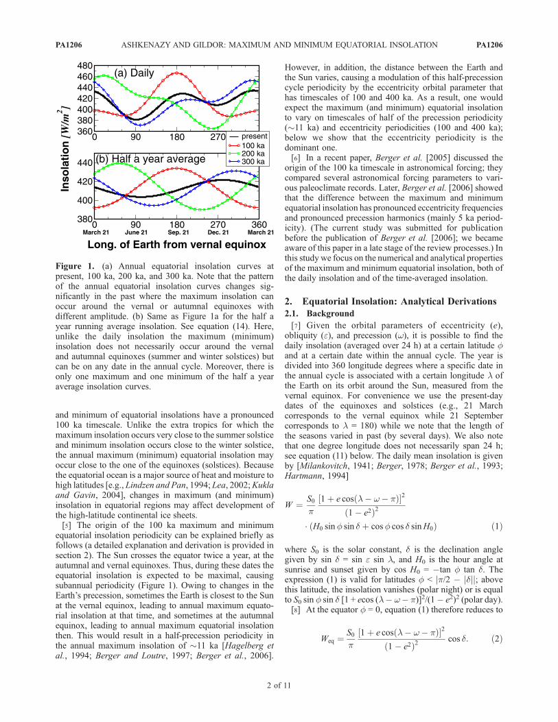
equatorial insolation periodicity can be explained briefly asfollows (a detailed explanation and derivation is provided insection 2). The Sun crosses the equator twice a year, at theautumnal and vernal equinoxes. Thus, during these dates theequatorial insolation is expected to be maximal, causingsubannual periodicity (Figure 1). Owing to changes in theEarth’s precession, sometimes the Earth is closest to the Sunat the vernal equinox, leading to annual maximum equato-rial insolation at that time, and sometimes at the autumnalequinox, leading to annual maximum equatorial insolationthen. This would result in a half-precession periodicity inthe annual maximum insolation of �11 ka [Hagelberg etal., 1994; Berger and Loutre, 1997; Berger et al., 2006].

However, in addition, the distance between the Earth andthe Sun varies, causing a modulation of this half-precessioncycle periodicity by the eccentricity orbital parameter thathas timescales of 100 and 400 ka. As a result, one wouldexpect the maximum (and minimum) equatorial insolationto vary on timescales of half of the precession periodicity(�11 ka) and eccentricity periodicities (100 and 400 ka);below we show that the eccentricity periodicity is thedominant one.[6] In a recent paper, Berger et al. [2005] discussed the

origin of the 100 ka timescale in astronomical forcing; theycompared several astronomical forcing parameters to vari-ous paleoclimate records. Later, Berger et al. [2006] showedthat the difference between the maximum and minimumequatorial insolation has pronounced eccentricity frequenciesand pronounced precession harmonics (mainly 5 ka period-icity). (The current study was submitted for publicationbefore the publication of Berger et al. [2006]; we becameaware of this paper in a late stage of the review processes.) Inthis study we focus on the numerical and analytical propertiesof the maximum and minimum equatorial insolation, both ofthe daily insolation and of the time-averaged insolation.

2. Equatorial Insolation: Analytical Derivations

2.1. Background

[7] Given the orbital parameters of eccentricity (e),obliquity (e), and precession (w), it is possible to find thedaily insolation (averaged over 24 h) at a certain latitude fand at a certain date within the annual cycle. The year isdivided into 360 longitude degrees where a specific date inthe annual cycle is associated with a certain longitude l ofthe Earth on its orbit around the Sun, measured from thevernal equinox. For convenience we use the present-daydates of the equinoxes and solstices (e.g., 21 Marchcorresponds to the vernal equinox while 21 Septembercorresponds to l = 180) while we note that the length ofthe seasons varied in past (by several days). We also notethat one degree longitude does not necessarily span 24 h;see equation (11) below. The daily mean insolation is givenby [Milankovitch, 1941; Berger, 1978; Berger et al., 1993;Hartmann, 1994]

W ¼ S0

p1þ e cos l� w� pð Þ½ �2

1� e2ð Þ2

H0 sinf sin d þ cosf cos d sinH0ð Þ ð1Þ

where S0 is the solar constant, d is the declination anglegiven by sin d = sin e sin l, and H0 is the hour angle atsunrise and sunset given by cos H0 = �tan f tan d. Theexpression (1) is valid for latitudes f < jp/2 � jdjj; abovethis latitude, the insolation vanishes (polar night) or is equalto S0 sin f sin d [1 + ecos (l� w� p)]2/(1� e2)2 (polar day).[8] At the equator f = 0, equation (1) therefore reduces to

Weq ¼S0

p1þ e cos l� w� pð Þ½ �2

1� e2ð Þ2cos d: ð2Þ

Figure 1. (a) Annual equatorial insolation curves atpresent, 100 ka, 200 ka, and 300 ka. Note that the patternof the annual equatorial insolation curves changes sig-nificantly in the past where the maximum insolation canoccur around the vernal or autumnal equinoxes withdifferent amplitude. (b) Same as Figure 1a for the half ayear running average insolation. See equation (14). Here,unlike the daily insolation the maximum (minimum)insolation does not necessarily occur around the vernaland autumnal equinoxes (summer and winter solstices) butcan be on any date in the annual cycle. Moreover, there isonly one maximum and one minimum of the half a yearaverage insolation curves.

PA1206 ASHKENAZY AND GILDOR: MAXIMUM AND MINIMUM EQUATORIAL INSOLATION

2 of 11

PA1206

Our aim is to estimate the annual maximum and minimumdaily insolation at the equator for a given time in the past;that is, for given orbital parameters e, e, and w we wish tofind a specific l that will yield the maximum (or minimum)insolation of the annual cycle.

2.2. Maximum and Minimum Equatorial Insolation:Rough Estimation

[9] The maximum insolation may be estimated by assum-ing cos(l � w � p) = 1, and that maximum equatorialinsolation tends to occur around the vernal and autumnalequinoxes (l = 0, p), cos d = 1. The approximatedmaximum equatorial insolation is thus

Weq;max ¼S0

p 1� eð Þ2� S0

p1þ 2eð Þ: ð3Þ

The right-hand side approximation is due to the fact thate � 1. Importantly, the estimated equatorial maximuminsolation depends only on the eccentricity orbital parameterthat has dominant frequencies with timescales of 100 ka and400 ka (Figure 2a).[10] We apply a similar approach to estimate the minimal

equatorial insolation within the annual cycle. To this end,we seek a l for which equation (2) is minimum, i.e., cos(l�w� p) =�1, and, since minimum equatorial insolation occuraround the solstices (l = p/2, 3p/2), cos d = cos e. Thus theminimum equatorial insolation may be estimated as

Weq;min ¼S0 cos e

p 1þ eð Þ2� S0 cos e

p1� 2eð Þ: ð4Þ

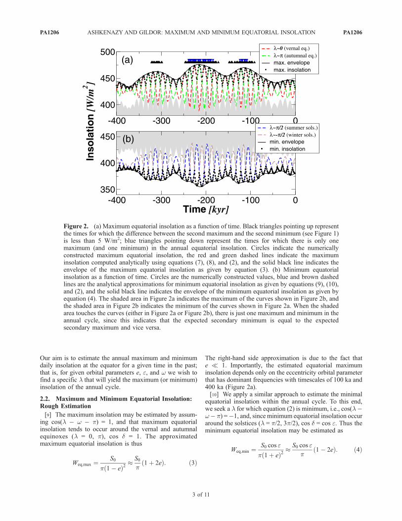
Figure 2. (a) Maximum equatorial insolation as a function of time. Black triangles pointing up representthe times for which the difference between the second maximum and the second minimum (see Figure 1)is less than 5 W/m2; blue triangles pointing down represent the times for which there is only onemaximum (and one minimum) in the annual equatorial insolation. Circles indicate the numericallyconstructed maximum equatorial insolation, the red and green dashed lines indicate the maximuminsolation computed analytically using equations (7), (8), and (2), and the solid black line indicates theenvelope of the maximum equatorial insolation as given by equation (3). (b) Minimum equatorialinsolation as a function of time. Circles are the numerically constructed values, blue and brown dashedlines are the analytical approximations for minimum equatorial insolation as given by equations (9), (10),and (2), and the solid black line indicates the envelope of the minimum equatorial insolation as given byequation (4). The shaded area in Figure 2a indicates the maximum of the curves shown in Figure 2b, andthe shaded area in Figure 2b indicates the minimum of the curves shown in Figure 2a. When the shadedarea touches the curves (either in Figure 2a or Figure 2b), there is just one maximum and minimum in theannual cycle, since this indicates that the expected secondary minimum is equal to the expectedsecondary maximum and vice versa.


3 of 11

PA1206

The estimated minimum equatorial insolation thus dependsmainly on eccentricity but also on obliquity (Figure 2a).[11] For typical values of S0 = 1350 W/m2, e = 23.5�

(cos e� 0.92) and e = 0.0046 to e = 0.049, the approximatedmaximum equatorial insolation ranges from 434 W/m2

to 475 W/m2, approximately 40 W/m2 difference. Thisdifference is large enough to influence the climate systemdynamics. The minimum equatorial insolation ranges from358 W/m2 for e = 0.049 to 390 W/m2 for e = 0.0046, about30 W/m2 difference. The difference between the maximumequatorial insolation and minimum equatorial insolationranges from 43 W/m2 for e = 0.0046 to 117 W/m2 for e =0.049; see Figures 2a and 2b.

2.3. Maximum and Minimum Equatorial Insolation:An Improved Approximation

[12] It is possible to accurately estimate the maximum andminimum equatorial insolations by taking into account thefact that the eccentricity orbital parameter and the obliquityangle are small, such that e � 1 and sin(e) � e (e is smallerthan 0.05 and e is less than 0.43 radian, 24.6�). In that caseequation (2) can be approximated as

~Weq �S0

p 1� e2ð Þ21� 2e cos l� wð Þ � 1

2e2 sin2 l

� �:

ð5Þ

The extremes can be found by differentiating equation (5)with respect to l and equating it to zero (@

~W eq/@l = 0):

2e sinl cosw� cosl sinwð Þ ¼ e2 sinl cosl: ð6Þ

The maximum equatorial insolation occurs around the vernaland autumnal equinoxes, l = 0 and l = p, while the minimumequatorial insolation occurs around the summer and wintersolstices, l = p/2 and l = 3p/2. Using in equation (6) theapproximations cosll�l* � cosl* � sinl*(l � l*) andsinll�l* � sin l* + cos l*(l � l*) for l* = 0, p/2, p, 3p/2we obtain the following:

l0 ¼sinw

� e22eþ cosw

for l � 0; ð7Þ

lp ¼ sinwe22eþ cosw

þ p for l � p; ð8Þ

lp2¼ � cosw

e22eþ sinw

þ p2

for l � p2; ð9Þ

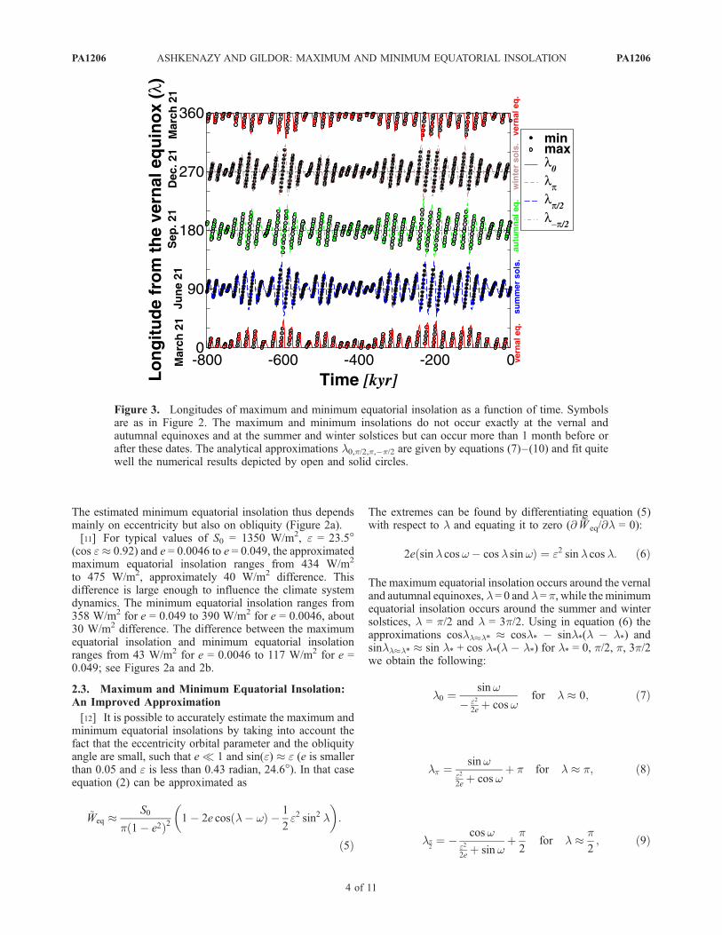
Figure 3. Longitudes of maximum and minimum equatorial insolation as a function of time. Symbolsare as in Figure 2. The maximum and minimum insolations do not occur exactly at the vernal andautumnal equinoxes and at the summer and winter solstices but can occur more than 1 month before orafter these dates. The analytical approximations l0,p/2,p,�p/2 are given by equations (7)–(10) and fit quitewell the numerical results depicted by open and solid circles.


4 of 11

PA1206

l�p2¼ � cosw

� e22eþ sinw

� p2

for l � �p2: ð10Þ

Once the different ‘‘dates’’ for the maximum and minimuminsolation are approximated it is possible to insert these lvalues into equation (2) to obtain the maximum andminimal equatorial insolations (see Figures 2 and 3).[13] The annual cycle of equatorial insolation usually has

two maximum and two minimum values. The expressionsabove provide these values at high accuracy where theinsolation curves associated with these l values have theprecession periodicity (Figures 2 and 3). However, a morerelevant measure may be the absolute maximum and min-imum insolation in the annual cycle. In that case, forexample, the longitude of the absolute maximum mayswitch from around the vernal equinox (l � 0) to aroundthe autumnal equinox (l � p/2), where this switching has aperiodicity of half of the precession cycle. Then, theeccentricity parameter will also be dominant, yieldingpronounced 100 ka and 400 ka periodicities (Figure 4); inaddition, the precession timescale will be replaced by a half-precession timescale.

2.4. Maximum and Minimum Equatorial Insolation:Time Average

[14] Heat and moisture transport from low to high lat-itudes are likely to influence the development of high-latitude ice sheets [Lindzen and Pan, 1994; Kukla andGavin, 2004]. These are not likely to be dictated by a singleday’s insolation but rather by the average insolation over

several months, a time period that can change the tropicalsea surface temperature and seasonality.[15] To evaluate the average insolation of a certain time

period within the annual cycle, it is necessary to calculate(1) the time lapse between the desired longitudes (measuredfrom the vernal equinox) based on Kepler’s second law and(2) the total insolation within this time period of the annualcycle. The derivative of the time lapse, t, with respect to thelongitude, l is given by [Milankovitch, 1941; Hartmann,1994]

dt

dl¼ 1� e2ð Þ2ffiffiffiffiffiffiffiffiffiffiffiffiffi

1� e2p 1

1þ e cos l� w� pð Þð Þ2

� 1� e2� �3=2

1þ 2e cos l� wð Þð Þ: ð11Þ

The time lapse between longitude l* � Dl to l* + Dl isthus

T ¼Z l*þDl

l*�Dl

dt

dldl

� 2 1� e2� �3=2

Dlþ 2e sinDl cos l*� wð Þð Þ: ð12Þ

The total insolation between longitude l* �Dl to l* +Dlusing equation (2) is

Z l*þDl

l*�DlWeq

dt

dldl � S0

pffiffiffiffiffiffiffiffiffiffiffiffiffi1� e2

p�2Dl

�1� e2

4

�

þ e2

4cos 2l* sin 2Dl

�: ð13Þ

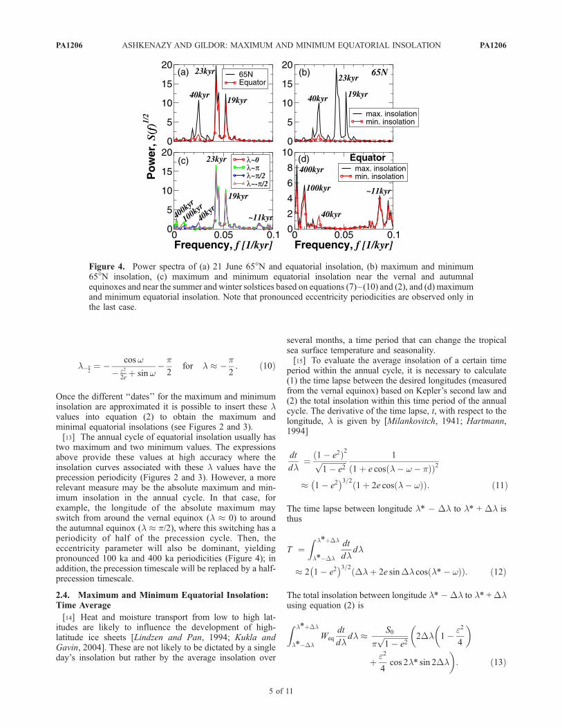
Figure 4. Power spectra of (a) 21 June 65�N and equatorial insolation, (b) maximum and minimum65�N insolation, (c) maximum and minimum equatorial insolation near the vernal and autumnalequinoxes and near the summer and winter solstices based on equations (7)–(10) and (2), and (d) maximumand minimum equatorial insolation. Note that pronounced eccentricity periodicities are observed only inthe last case.


5 of 11

PA1206

(Note that total insolation between any two longitudes isindependent of precession [e.g., Milankovitch, 1941; Loutreet al., 2004; Paillard, 2001; Huybers, 2006]). Thus theaverage insolation between longitudel*�Dl andl* +Dl is

W eq ¼1

T

Z l*þDl

l*�DlWeq

dt

dldl � S0

p 1� e2ð Þ2

��1þ e2

4

�cos 2l*

sin 2Dl2Dl

� 1

�

� 2esinDlDl

cos l*� w��

: ð14Þ�

When Dl � 1 (daily average insolation), equation (14)reduces to equation (5), since in that case sin Dl/Dl ! 1.[16] As in the previous subsection, to find the maximum

and minimum of the equatorial time averaged insolation it isnecessary to differentiate W eq with respect to l* and toequate it to zero (@W eq/@l* = 0). The equation to be solved is

2esinDlDl

sinl* cosw� cosl* sinwð Þ

¼ e2sin 2Dl2Dl

sinl* cosl*: ð15Þ

This equation is similar to equation (6) and the l*0,p,±p/2 forequation (15) are the same as in equations (7)–(10) where thefactor e2

2eshould be replaced by (e

2

2e) cos Dl. Then these

l*0,p,±p/2 should be used in equation (14) to find the maximaand minima of the averaged equatorial insolation.[17] When averaging over a longer period in the annual

cycle (i.e., larger Dl), the factor sinDlDl becomes smaller and

smaller, and thus the contribution of the precession orbitalparameter in cos(l* � w) in equation (14) also becomessmaller. Using the average insolation over a period ofseveral months may better represent the ocean because of itslarge heat capacity; the oceans act to ‘‘integrate’’ the effectof insolation over many days. For the special case of 6months averaging period (Dl = p/2), the average insolationover the time period between l* � p/2 to l* + p/2(equation (14)) is

W eq Dl ¼ p2

� �¼ S0

p 1� e2ð Þ21� e2

4� 4e

pcos l*� wð Þ

� �:

ð16Þ

In this case the maximum of the average equatorial insolationoccurs for cos(l* � w) = �1 (or l* = w + p) and is

W eq;max Dl ¼ p2

� �¼ S0

p 1� e2ð Þ21� e2

4þ 4e

p

� �

�S0 1� e2

4

� �

1� e2ð Þ2 p� 4eð Þ: ð17Þ

The minimum of the average equatorial insolation occurs forcos(l* � w) = 1 (or l* = w) and is

W eq;min Dl ¼ p2

� �¼ S0

p 1� e2ð Þ21� e2

4� 4e

p

� �

�S0 1� e2

4

� �

1� e2ð Þ2 pþ 4eð Þ: ð18Þ

Unlike the daily insolation, for the half a year averageequatorial insolation there is only one annual maximum andminimumwhere the relative phase between these two is half ayear (Figure 1b). Since the Earth’s position with respect to theperihelion, n, is n = l � w � p [Berger, 1978; Berger et al.,1993], the maximum of the half a year average equatorialinsolation occurs for l* that coincides with the perihelion(the point on the Earth’s orbit that is the closest to the Sun),while the minimum of the half a year average equatorialinsolation occurs for l* that coincides with the aphelion (thepoint on the Earth’s orbit that is the farthest from the Sun).[18] Thus the maximum and minimum of the half a year

average equatorial insolation depend mainly on the eccen-tricity orbital parameter and are independent of the preces-sion parameter. We thus expect the maximum and minimumof the half a year equatorial insolation to have pronounced400 ka and 100 ka timescales (eccentricity timescales), aweaker 40 ka timescale (obliquity timescale), and no�20 kaor �11ka timescale (semiprecession timescale) (Figures 5and 6).

3. Equatorial Insolation: Results

[19] One of the differences between the tropics and theextratropics is that the Sun crosses the equator twice a yearcausing maximum insolation around the vernal and autum-nal equinoxes and minimum insolation around the summerand winter solstices. On the other hand, in the NH (SH)extra tropics, maximum insolation occurs around the sum-mer (winter) solstice while minimum insolation occursaround the winter (summer) solstice. In Figure 1a we showthe equatorial annual cycle of insolation during the present,100 ka ago, 200 ka, and 300 ka. The maximum insolationaround the vernal equinox is sometimes larger than themaximum insolation around the autumnal equinox and viceversa. Moreover, in some cases there is just one maximumand minimum in the annual cycle of the equatorial insola-tion. This occurred, for example, 200 ka, where there wasonly one maximum insolation around the vernal equinoxand only one minimum insolation around the winter solstice.[20] The case of the half-year (running) average is differ-

ent consistently with only one maximum and one minimumduring the year. However, the maximum and minimuminsolations can occur at any date in the annual cycle (seeFigure 1b) in contrast to the extratropics, where they occurclose to the summer and winter solstices.[21] In order to understand more deeply the changes in the

maximum equatorial insolation we show in Figure 2a (1) the


6 of 11

PA1206

numerically extracted maximal equatorial insolation curves,(2) the maximum equatorial insolation around the vernaland autumnal equinox, and (3) the ‘‘envelope’’ of themaximum insolation (equation (3)). The agreement betweenthe ‘‘numerically’’ extracted maximum equatorial insolationand those given by equations (2), (7), and (8) is very goodand supports the approximations that were assumed toderive these expressions. The maximum insolation thatoccurs around the vernal and autumnal equinoxes has thetimescales of the precession orbital parameter (i.e., 19 and23 ka), where these two curves have a relative phase of halfof the precession cycle, approximately 11 ka. Thus, whenconsidering just the maximal value of these two, a period-icity of �11 ka is expected. These 11 ka cycles aremodulated by the much slower frequency of the eccentricityforcing as given by equation (3) and depicted in Figure 2a.Note that the obliquity frequency of �40 ka does not playany role here.[22] We also plot the insolation curves of minimum

insolation (Figure 2b) in a similar way to the maximuminsolation which is plotted in Figure 2a. The minimalequatorial curves have similar features as the maximumequatorial curves depicted in Figure 2a. The notable differ-ence is that the envelope of the minimal insolation has atimescale of the obliquity orbital parameter that is given byequation (4). Still, this obliquity timescale of �40 ka is notpronounced and the dominant frequencies are that of theeccentricity (400 and 100 ka) and precession (23 and 19 ka)orbital parameters.

[23] Although the Sun crosses the equator twice a year,the equatorial insolation curves do not always have twominimum and two maximum insolation points in the annualcycles. This happens when the approximated minimuminsolation given by equations (2), (9), and (10) is largerthan the approximated maximum insolation given by equa-tions (2), (7), and (8). We denoted these times by a bluetriangle pointed down in Figure 2a, and it is clear that suchsituations occur when the eccentricity orbital parameter islarge (e.g., the time period between 240 ka and 183 ka);there are 55 such points in the time interval between 400 kato present. (When the eccentricity parameter is large, theEarth may be sufficiently far from the Sun during theequinoxes (at which the equatorial insolation is expectedto be maximal), weakening the insolation compares to otherdates in the annual cycle.)[24] In Figure 3, we plot the longitudes of the Earth

relative to the vernal equinox at which the maximum andminimum insolations occur. Also here the agreement be-tween the longitudes given by equations (7)–(10) is veryclose to the ones numerically constructed by locating themaximum and minimum equatorial insolation from theannual insolation curves. It is also clear that the maximumequatorial insolation does indeed occur around the vernaland autumnal equinoxes while the minimum equatorialinsolation occurs around the summer and winter solstices;the deviations may be as large as 1 and a half months.[25] To demonstrate the difference between the insolation

at the equatorial region and the nonequatorial regions, we

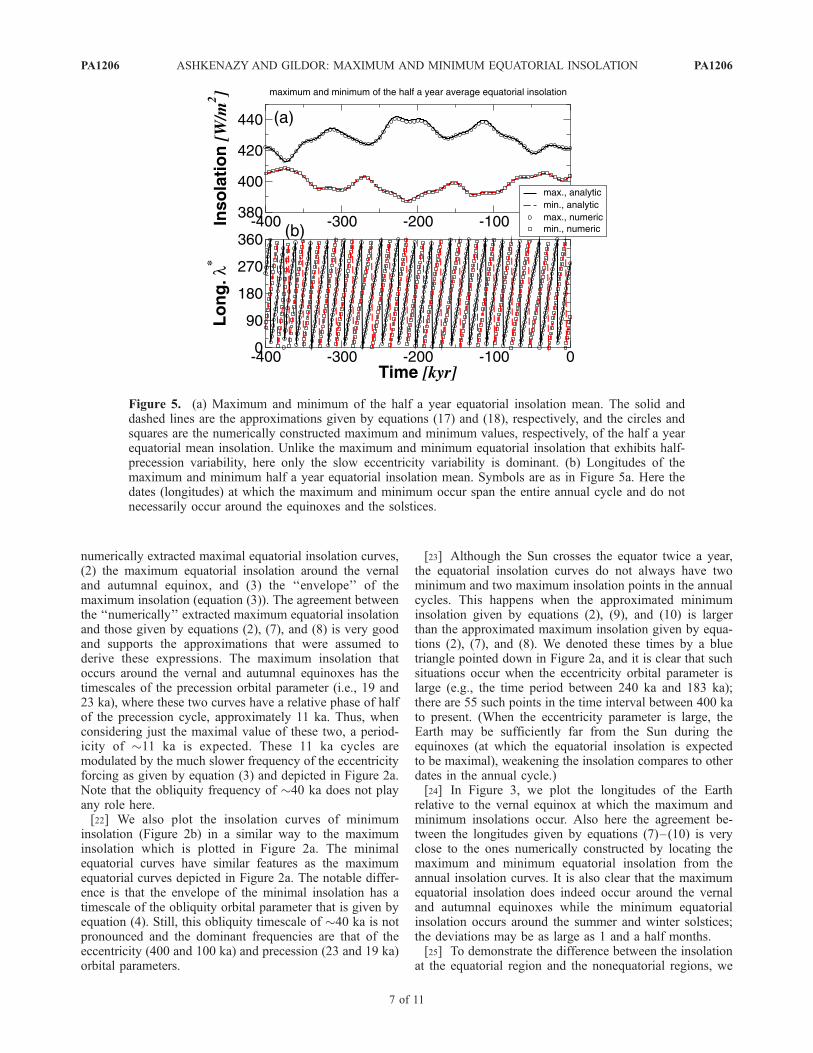
Figure 5. (a) Maximum and minimum of the half a year equatorial insolation mean. The solid anddashed lines are the approximations given by equations (17) and (18), respectively, and the circles andsquares are the numerically constructed maximum and minimum values, respectively, of the half a yearequatorial mean insolation. Unlike the maximum and minimum equatorial insolation that exhibits half-precession variability, here only the slow eccentricity variability is dominant. (b) Longitudes of themaximum and minimum half a year equatorial insolation mean. Symbols are as in Figure 5a. Here thedates (longitudes) at which the maximum and minimum occur span the entire annual cycle and do notnecessarily occur around the equinoxes and the solstices.


7 of 11

PA1206

plotted the power frequency spectra of different insolationcurves. In Figure 4a we plotted the power spectrum of theinsolation curve of the summer solstice at 65 �N and at theequator. In both curves the eccentricity frequency of 100 kais very weak. However, while for 65�N there is a significantobliquity frequency of �40 ka it is much weaker at theequator; note that the annual mean equatorial insolation hasa dominant obliquity periodicity with variability of severalW/m2. The maximum insolation at 65�N presented inFigure 4b has almost the same power spectrum as inFigure 4a; this similarity is expected since the maximuminsolation at 65�N occurs very close to the summer solstice.On the other hand, as expected, the minimum insolation at65�N has very weak power with a dominant obliquityfrequency. In Figure 4c we present the power spectra ofthe equatorial insolation curves given by equations (2) and(7)–(10). Also here as in Figure 4a the dominant frequencyis the precession frequency; nevertheless, the frequencyassociated with the obliquity and eccentricity orbital param-eters starts to emerge. The pronounced precession frequencyis due to the oscillatory behavior of these curves as shown inFigure 2a. It is only when considering the maximum andminimum of equatorial insolation that the eccentricityfrequencies become the dominant ones (Figure 4d). In thiscase the precession frequencies are replaced by double their

values, with a timescale of �11 ka instead of �20 ka. Theminimum equatorial insolation curve also has the obliquityfrequency (equations 3 and 4).[26] As discussed in section 2.4, if changes in equatorial

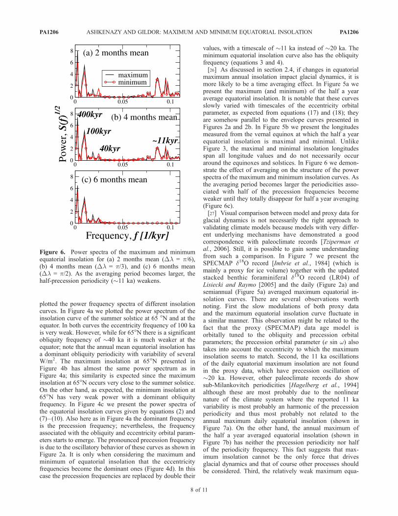
maximum annual insolation impact glacial dynamics, it ismore likely to be a time averaging effect. In Figure 5a wepresent the maximum (and minimum) of the half a yearaverage equatorial insolation. It is notable that these curvesslowly varied with timescales of the eccentricity orbitalparameter, as expected from equations (17) and (18); theyare somehow parallel to the envelope curves presented inFigures 2a and 2b. In Figure 5b we present the longitudesmeasured from the vernal equinox at which the half a yearequatorial insolation is maximal and minimal. UnlikeFigure 3, the maximal and minimal insolation longitudesspan all longitude values and do not necessarily occuraround the equinoxes and solstices. In Figure 6 we demon-strate the effect of averaging on the structure of the powerspectra of the maximum and minimum insolation curves. Asthe averaging period becomes larger the periodicities asso-ciated with half of the precession frequencies becomeweaker until they totally disappear for half a year averaging(Figure 6c).[27] Visual comparison between model and proxy data for

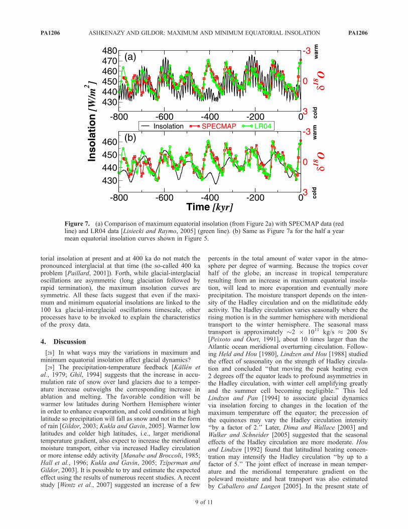
glacial dynamics is not necessarily the right approach tovalidating climate models because models with very differ-ent underlying mechanisms have demonstrated a goodcorrespondence with paleoclimate records [Tziperman etal., 2006]. Still, it is possible to gain some understandingfrom such a comparison. In Figure 7 we present theSPECMAP d18O record [Imbrie et al., 1984] (which ismainly a proxy for ice volume) together with the updatedstacked benthic foraminiferal d18O record (LR04) ofLisiecki and Raymo [2005] and the daily (Figure 2a) andsemiannual (Figure 5a) averaged maximum equatorial in-solation curves. There are several observations worthnoting. First the slow modulations of both proxy dataand the maximum equatorial insolation curve fluctuate ina similar manner. This observation might be related to thefact that the proxy (SPECMAP) data age model isorbitally tuned to the obliquity and precession orbitalparameters; the precession orbital parameter (e sin w) alsotakes into account the eccentricity to which the maximuminsolation seems to match. Second, the 11 ka oscillationsof the daily equatorial maximum insolation are not foundin the proxy data, which have precession oscillation of�20 ka. However, other paleoclimate records do showsub-Milankovitch periodicities [Hagelberg et al., 1994]although these are most probably due to the nonlinearnature of the climate system where the reported 11 kavariability is most probably an harmonic of the precessionperiodicity and thus most probably not related to theannual maximum daily equatorial insolation (shown inFigure 7a). On the other hand, the annual maximum ofthe half a year averaged equatorial insolation (shown inFigure 7b) has neither the precession periodicity nor halfof the periodicity frequency. This fact suggests that max-imum insolation cannot be the only force that drivesglacial dynamics and that of course other processes shouldbe considered. Third, the relatively weak maximum equa-

Figure 6. Power spectra of the maximum and minimumequatorial insolation for (a) 2 months mean (Dl = p/6),(b) 4 months mean (Dl = p/3), and (c) 6 months mean(Dl = p/2). As the averaging period becomes larger, thehalf-precession periodicity (�11 ka) weakens.


8 of 11

PA1206

torial insolation at present and at 400 ka do not match thepronounced interglacial at that time (the so-called 400 kaproblem [Paillard, 2001]). Forth, while glacial-interglacialoscillations are asymmetric (long glaciation followed byrapid termination), the maximum insolation curves aresymmetric. All these facts suggest that even if the maxi-mum and minimum equatorial insolations are linked to the100 ka glacial-interglacial oscillations timescale, otherprocesses have to be invoked to explain the characteristicsof the proxy data.

4. Discussion

[28] In what ways may the variations in maximum andminimum equatorial insolation affect glacial dynamics?[29] The precipitation-temperature feedback [Kallen et

al., 1979; Ghil, 1994] suggests that the increase in accu-mulation rate of snow over land glaciers due to a temper-ature increase outweighs the corresponding increase inablation and melting. The favorable condition will bewarmer low latitudes during Northern Hemisphere winterin order to enhance evaporation, and cold conditions at highlatitude so precipitation will fall as snow and not in the formof rain [Gildor, 2003; Kukla and Gavin, 2005]. Warmer lowlatitudes and colder high latitudes, i.e., larger meridionaltemperature gradient, also expect to increase the meridionalmoisture transport, either via increased Hadley circulationor more intense eddy activity [Manabe and Broccoli, 1985;Hall et al., 1996; Kukla and Gavin, 2005; Tziperman andGildor, 2003]. It is possible to try and estimate the expectedeffect using the results of numerous recent studies. A recentstudy [Wentz et al., 2007] suggested an increase of a few

percents in the total amount of water vapor in the atmo-sphere per degree of warming. Because the tropics coverhalf of the globe, an increase in tropical temperatureresulting from an increase in maximum equatorial insola-tion, will lead to more evaporation and eventually moreprecipitation. The moisture transport depends on the inten-sity of the Hadley circulation and on the midlatitude eddyactivity. The Hadley circulation varies seasonally where therising motion is in the summer hemisphere with meridionaltransport to the winter hemisphere. The seasonal masstransport is approximately �2 � 1011 kg/s � 200 Sv[Peixoto and Oort, 1991], about 10 times larger than theAtlantic ocean meridional overturning circulation. Follow-ing Held and Hou [1980], Lindzen and Hou [1988] studiedthe effect of seasonality on the strength of Hadley circula-tion and concluded ‘‘that moving the peak heating even2 degrees off the equator leads to profound asymmetries inthe Hadley circulation, with winter cell amplifying greatlyand the summer cell becoming negligible.’’ This ledLindzen and Pan [1994] to associate glacial dynamicsvia insolation forcing to changes in the location of themaximum temperature off the equator; the precession ofthe equinoxes may vary the Hadley circulation intensity‘‘by a factor of 2.’’ Later, Dima and Wallace [2003] andWalker and Schneider [2005] suggested that the seasonaleffects of the Hadley circulation are more moderate. Houand Lindzen [1992] found that latitudinal heating concen-tration may intensify the Hadley circulation ‘‘by up to afactor of 5.’’ The joint effect of increase in mean temper-ature and the meridional temperature gradient on thepoleward moisture and heat transport was also estimatedby Caballero and Langen [2005]. In the present state of

Figure 7. (a) Comparison of maximum equatorial insolation (from Figure 2a) with SPECMAP data (redline) and LR04 data [Lisiecki and Raymo, 2005] (green line). (b) Same as Figure 7a for the half a yearmean equatorial insolation curves shown in Figure 5.


9 of 11

PA1206

the climate system, an increase in mean temperature and/ormeridional temperature gradient will significantly increasemeridional heat and moisture transport.[30] The above studies suggest that relatively small

changes in the pattern of the maximum zonally averagedtropical temperature may result in drastic changes in Hadleycirculation. It is plausible that as maximum equatorialinsolation increases, the timing and concentration of themaximum zonally averaged temperature will change inaccord, which will drastically affect the intensity of thewinter cell Hadley circulation. Changes in Hadley circula-tion intensity may increase the midlatitude cyclone activitywhich acts to moderate the meridional temperature gradientand hence affects the buildup and melting of the highnorthern latitude ice sheets. Together with other mechanisms,the maximum equatorial insolation thus may lead to theglacial-interglacial oscillations and to the 100 ka timescale.[31] The equatorial region plays an important role in

climate dynamics and may affect glacial dynamics as well[Cane, 1998]. Among other phenomena unique to theequatorial region (like the El Nino) are changes in equato-rial insolation. Unlike high latitudes, where maximuminsolation occurs around the summer solstice and minimuminsolation occurs around the winter solstice, the insolation atthe equator is sometimes maximal around the vernal equi-nox, sometimes maximal around the autumnal equinox,sometimes with only one annual maximum and one annualminimum, and sometimes with two similar maxima and twosimilar minima in an annual cycle. This behavior is char-acterized by periodicities of 400, 100 and 11 ka. We havedeveloped analytical expressions to describe the maximumand minimum equatorial insolation.[32] We have also shown that when dealing with the

maximum and minimum of the time averaged equatorialinsolation, the half-precession periodicity becomes weakerand weaker and that it disappears for the maximum andminimum of the half a year equatorial insolation. It is morelikely that the time mean equatorial insolation affects large-scale climate dynamics because SST would not respondimmediately to daily insolation changes. Thus the half-precession cycle periodicity will not be pronounced in proxyrecords in part because of the response time of the oceansurface and in part because of other climate feedbacks.[33] The direct effect of changing tropical insolation may

be the warming or cooling of SST. This may stimulate

various processes in the climate system that compete witheach other and eventually cause changes in high latitudes aswell. For example, the tropics, and especially the westernPacific, are a ‘‘heat engine’’ [Lea, 2002] and moisturesource to high latitudes. The warm pool in the westernequatorial Pacific has the highest SST of the ocean and ischaracterized by a substantial amount of warming trans-ferred to high latitudes by atmospheric processes [Peixotoand Oort, 1991]. Alternation of this heat/moisture sourcemay affect the buildup and melting of the large NorthernHemisphere (NH) continental ice sheets [e.g., Lindzen andPan, 1994; Kukla and Gavin, 2004, 2005]. Variations in themaximum and minimum equatorial insolation may alsoaffect ENSO and its frequency [Cane, 1998; Bronnimannet al., 2004; Kukla et al., 2002; Kukla and Gavin, 2005]. Inaddition, equatorial heat is carried to higher latitudes via thewestern boundary currents (the Gulf stream and the Kur-oshio current) and the thermohaline (overturning) circula-tion. These two may affect each other through variousfeedback mechanisms [Pasquero and Tziperman, 2004].Similarly, the monsoons, the Hadley cell circulation, andthe meridional wind pattern may be changed as the maxi-mum (and minimum) equatorial insolation changes and inthis way to affect glacial dynamics. Further studies areneeded to explore in more detail the potential effect of theannual maximum and minimum equatorial insolation on theclimate system and on glacial dynamics.[34] Various mechanisms have been proposed to explain

the glacial-interglacial oscillations of the last 800 ka. Thecommon feature is that the 100 ka glacial cycle is notdirectly caused by insolation changes. Here we suggest thatthe 100 ka cycle might be linked to the annual maximumand minimum equatorial insolation. Even in this case,however, other feedbacks and mechanisms have to beincluded in order to explain the characteristics of the glacialcycles, such as the asymmetry of glacial-interglacial oscilla-tion (rapid deglaciation that is followed by slow glaciation)and the presence of a precession timescale in proxy records.

[35] Acknowledgments. We thank Gerald Dickens, David Lea, EliTziperman, and two anonymous reviewers for helpful discussions. Thisresearch was supported by the U.S.-Israel Binational Science Foundation.Y.A. is supported by the Israeli Center for Complexity Science. H.G. isthe Incumbent of the Rowland and Sylvia Schaefer Career DevelopmentChair.


10 of 11

PA1206

ReferencesAdhemar, J. A. (1842), Revolutions de la Mer:Deluges Periodiques, Carilian-Goeury et V.Dalmont, Paris.

Ashkenazy, Y., and E. Tziperman (2004), Are the41 kyr glacial oscillations a linear response toMilankovitch forcing?, Quat. Sci. Rev., 23,1879–1890.

Berger, A. (1978), Long-term variations of dailyinsolation and Quaternary climate changes,J. Atmos. Sci., 35, 2362–2367.

Berger, A., and M. F. Loutre (1996), Model-ing the climate response to astronomical andCO2 forcing, C. R. Acad. Sci. Paris, 323, 1–16.

Berger, A., and M. F. Loutre (1997), Intertropicallatitudes and precessional and half-preces-sional cycles, Science, 278, 1476–1478.

Berger, A., M. F. Loutre, and C. Tricot (1993),Insolation of Earth’s orbital periods, J. Geo-phys. Res., 98, 10,341–10,362.

Berger, A., J. L. Melice, and M. F. Loutre (2005),On the origin of the 100-kyr cycles in the as-tronomical forcing, Paleoceanography, 20,PA4019, doi:10.1029/2005PA001173.

Berger, A., M. F. Loutre, and J. L. Melice (2006),Equatorial insolation: From precession harmo-nics to eccentricity frequencies, Clim. Past, 2,131–136.

Bronnimann, S., J. Luterbacher, J. Staehelin, T.M.Svendby, G. Hansen, and T. Svenoe (2004),Extreme climate of the global troposphere andstratosphere in 1940–42 related to El Nino,Nature, 431, 971–974.

Caballero, R., and P. L. Langen (2005), The dy-namic range of poleward energy transport in anatmospheric general circulation model, Geo-phys. Res. Lett., 32, L02705, doi:10.1029/2004GL021581.

Cane, M. A. (1998), Climate change: A role forthe tropical Pacific, Science, 282, 59–61.

Clement, A. C., R. Seager, and M. A. Cane(1999), Orbital controls on the El Nino/South-


11 of 11

PA1206

ern Oscillation and the tropical climate, Paleo-ceanography, 14, 441–456.

Croll, J. (1875), Climate and Time in TheirGeological Relations: A Theory of SecularChanges of the Earth’s Climate, Appleton,New York.

Dima, I. M., and J. M. Wallace (2003), On theseasonality of the Hadley cell, J. Atmos. Sci.,60, 1522–1527.

Ghil, M. (1994), Cryothermodynamics: Thechaotic dynamics of paleoclimate, Physica D,77, 130–159.

Gildor, H. (2003), When Earth’s freezer door isleft ajar, Eos Trans. AGU, 84, 215.

Gildor, H., and E. Tziperman (2000), Sea ice asthe glacial cycles climate switch: Role of sea-sonal and orbital forcing, Paleoceanography,15, 605–615.

Hagelberg, T. K., G. Bond, and P. deMenocal(1994), Milankovitch band forcing of sub-Milankovitch climate variability during thePleistocene, Paleoceanography, 9, 545 –558.

Hall, N. M. J., P. J. Valdes, and B. Dong (1996),The maintenance of the last great ice sheets: AUGAMP GCM study, J. Clim., 9, 1004–1019.

Hartmann, D. (1994), Global Physical Climatol-ogy, Academic, San Diego, Calif.

Held, I. M., and A. Y. Hou (1980), Non-linearaxially-symmetric circulations in a nearly invis-cid atmosphere, J. Atmos. Sci., 37, 515–533.

Hou, A. Y., and R. S. Lindzen (1992), The influ-ence of concentrated heating on the Hadleycirculation, J. Atmos. Sci., 49, 1233–1241.

Huybers, P. (2006), Early Pleistocene glacial cy-cles and the integrated summer insolation for-cing, Science, 28, 508–511.

Imbrie, J., J. Hays, D. Martinson, A. McIntyre, A.Mix, J. Morley, N. Pisias, W. Prell, and N.Shackleton (1984), The orbital theory of Pleis-tocene climate: Support from a revised chron-ology of the mar ine d18O record , inMilankovitch and Climate, Part I, NATO ASISer., Ser. C, vol. 126, edited by A. Berger et al.,pp. 269–305,D.Reidel, Dordrecht,Netherlands.

Imbrie, J., et al. (1993), On the structure and originof major glaciation cycles: 2. The 100,000-yearcycle, Paleoceanography, 8, 699–735.

Kallen, E., C. Crafoord, and M. Ghil (1979), Freeoscillations in a climate model with ice-sheetdynamics, J. Atmos. Sci., 36, 2292–2303.

Kukla, G., and J. Gavin (2004), Milankovitchclimate reinforcements, Global Planet. Change,40, 27–48.

Kukla, G., and J. Gavin (2005), Did glacials startwith global warming?, Quat. Sci. Rev., 24,1547–1557.

Kukla, G. J., A. C. Clement, M. A. Cane, J. E.Gavin, and S. E. Zebiak (2002), Last interglacialand early glacial ENSO, Quat. Res., 58, 27–31.

Laskar, J. (1990), The chaotic motion of the solarsystem: A numerical estimate of the chaoticzones, Icarus, 88, 266–291.

Laskar, J., F. Joutel, and F. Boudin (1993), Orbi-tal, precessional, and insolation quantities forthe Earth from �20 Myr to +10 Myr, Astron.Astrophys., 270, 522–533.

Lea, D. W. (2002), Paleoclimate: The glacial tro-pical Pacific – not just a west side story,Science, 297, 202–203.

Lea, D. W. (2004), The 100,000-yr cycle in tro-pical SST, greenhouse forcing, and climatesensitivity, J. Clim., 17, 2170–2179.

Lindzen, R. S., and A. Y. Hou (1988), Hadley cir-culations for zonally averaged heating centeredoff the equator, J. Atmos. Sci., 45, 2416–2427.

Lindzen, R. S., and W. W. Pan (1994), A note onorbital control of equator-pole heat fluxes,Clim. Dyn., 10, 49–57.

Lisiecki, L. E., and M. E. Raymo (2005), APliocene-Pleistocene stack of 57 globally dis-tributed benthic d18O records, Paleoceanogra-phy, 20, PA1003, doi:10.1029/2004PA001071.

Loutre, M.-F., D. Paillard, F. Vimeux, and E. Cortijo(2004), Does mean annual insolation have thepotential to change the climate?, Earth Planet.Sci. Lett., 221, 1–14.

Manabe, S., and A. J. Broccoli (1985), A com-parison of climate model sensitivity with datafrom the Last Glacial Maximum, J. Atmos.Sci., 42, 2643–2651.

Milankovitch, M. (1941), Canon of Insolationand the Ice-Age Problem (in German), Spec.Publ., vol. 132, R. Serb. Acad., Belgrade.(English translation, Israel Program for Sci.Transl., Jerusalem, 1969.)

Paillard, D. (1998), The timing of Pleistoceneglaciations from a simple multiple-state cli-mate model, Nature, 391, 378–381.

Paillard, D. (2001), Glacial cycles: Toward a newparadigm, Rev. Geophys., 39, 325–346.

Pasquero, C., and E. Tziperman (2004), Effects ofa wind driven gyre on thermohaline circulationvariability, J. Phys. Oceanogr., 34, 805–816.

Peixoto, J., and A. Oort (1991), Physics of Cli-mate, Am. Inst. of Phys., New York.

Rubincam, D. P. (2004), Black body tempera-ture, orbital elements, the Milankovitch preces-

sion index, and the Seversmith psychroterms,Theor. Appl. Climatol., 79, 111–131.

Saltzman, B. (1987), Carbon dioxide and the d18Orecord of late-Quaternary climatic change: Aglobal model, Clim. Dyn., 1, 77–85.

Saltzman, B. (1990), Three basic problems ofpaleoclimatic modeling: A personal perspec-tive and review, Clim. Dyn., 5, 67–78.

Saltzman, B., and A. Sutera (1984), A model ofthe internal feedback system involved in LateQuaternary climatic variations, J. Atmos. Sci.,41, 736–745.

Short, D. A., J. G. Mengel, T. J. Crowley, W. T.Hyde, and G. R. North (1991), Filtering ofMilankovitch cycles by Earth’s geography,Quat. Res., 35, 157–173.

Timmermann, A., S. J. Lorenz, S.-I. An,A. Clement, and S.-P. Xie (2007), The effectof orbital forcing on the mean climate andvariability of the tropical Pacific, J. Clim.,20, 4147–4159.

Tziperman, E., and H. Gildor (2003), Themid-Pleistocene climate transition to 100-kyrglacial cycles and the asymmetry between gla-ciation and deglaciation times, Paleoceanogra-phy, 18(1), 1001, doi:10.1029/2001PA000627.

Tziperman, E., M. Raymo, P. Huybers, andC. Wunsch (2006), Consequences of pacingthe pleistocene 100 kyr ice ages by non-linear phase locking to Milankovitch for-cing, Paleoceanography, 21, PA4206,doi:10.1029/2005PA001241.

Walker, C. C., and T. Schneider (2005), Re-sponse of idealized Hadley circulations to sea-sonally varying heating, Geophys. Res. Lett.,32, L06813, doi:10.1029/2004GL022304.

Wentz, F. J., L. Ricciardulli, K. Hilburn, andC. Mears (2007), How much more rain willglobal warming bring?, Science, 317, 232–235, doi:10.1126/science.1140746.

��Y. Ashkenazy, Department of Solar Energy

and Environmental Physics, The J. BlausteinInstitutes for Desert Research, Ben Gurion Uni-versity of the Negev, Sede Boqer Campus,Midreshet Ben-Gurion 84990, Israel. ([email protected])H. Gildor, Department of Environmental

Sciences, Weizmann Institute of Science, Reho-vot 76100, Israel. ([email protected])

Timing and significance of maximum and minimum equatorial insolation

Documents

Transcript of Timing and significance of maximum and minimum equatorial insolation