Optimization approaches for minimum conductance graph ...
137
HAL Id: tel-03484309 https://tel.archives-ouvertes.fr/tel-03484309 Submitted on 17 Dec 2021 HAL is a multi-disciplinary open access archive for the deposit and dissemination of sci- entific research documents, whether they are pub- lished or not. The documents may come from teaching and research institutions in France or abroad, or from public or private research centers. L’archive ouverte pluridisciplinaire HAL, est destinée au dépôt et à la diffusion de documents scientifiques de niveau recherche, publiés ou non, émanant des établissements d’enseignement et de recherche français ou étrangers, des laboratoires publics ou privés. Optimization approaches for minimum conductance graph partitioning Zhi Lu To cite this version: Zhi Lu. Optimization approaches for minimum conductance graph partitioning. Optimization and Control [math.OC]. Université d’Angers, 2020. English. NNT : 2020ANGE0013. tel-03484309
-
Upload
khangminh22 -
Category
Documents
-
view
0 -
download
0
Transcript of Optimization approaches for minimum conductance graph ...

HAL Id: tel-03484309https://tel.archives-ouvertes.fr/tel-03484309
Submitted on 17 Dec 2021
HAL is a multi-disciplinary open accessarchive for the deposit and dissemination of sci-entific research documents, whether they are pub-lished or not. The documents may come fromteaching and research institutions in France orabroad, or from public or private research centers.
L’archive ouverte pluridisciplinaire HAL, estdestinée au dépôt et à la diffusion de documentsscientifiques de niveau recherche, publiés ou non,émanant des établissements d’enseignement et derecherche français ou étrangers, des laboratoirespublics ou privés.
Optimization approaches for minimum conductancegraph partitioning
Zhi Lu
To cite this version:Zhi Lu. Optimization approaches for minimum conductance graph partitioning. Optimization andControl [math.OC]. Université d’Angers, 2020. English. NNT : 2020ANGE0013. tel-03484309

THÈSE DE DOCTORAT DE
L’UNIVERSITÉ D’ANGERSCOMUE UNIVERSITÉ BRETAGNE LOIRE
ÉCOLE DOCTORALE N° 601Mathématiques et Sciences et Technologiesde l’Information et de la CommunicationSpécialité : Informatique
Par
Zhi LUOptimization Approaches for Minimum Conductance GraphPartitioning
Thèse présentée et soutenue à Angers, le 08 Juillet 2020Unité de recherche : Laboratoire d’Étude et de Recherche en Informatique d’Angers (LERIA)Thèse N° :
Rapporteurs avant soutenance :
M. Patrick DE CAUSMAECKER Professeur, KU LeuvenM. Chumin LI Professeur, Université de Picardie Jules Verne
Composition du Jury :
Président : Mme. Béatrice DUVAL Professeur, Université d’AngersExaminateurs : M. Patrick DE CAUSMAECKER Professeur, KU Leuven
Mme. Béatrice DUVAL Professeur, Université d’AngersM. Chumin LI Professeur, Université de Picardie Jules Verne
Directeur de thèse : M. Jin-Kao HAO Professeur, Université d’Angers


ACKNOWLEDGEMENT
I would like to express my sincere gratitude to my supervisor Prof. Jin-Kao Hao,who introduced me to the incredibly interesting combinatorial optimization problems. Iappreciate all his contributions of time, advice, and patience to make my Ph.D. experienceproductive and meaningful.
I also thank all the jury members, for their efforts to advancing this thesis and writingthoughtful review reports.
With many thanks to my colleagues at LERIA, University of Angers, for the stimu-lating discussions, and for the good time we were working together.
My sincere thanks also goes to my best friends from China and France, for the warmththey extended to me, and for the wonderful time we shared.
I would like to thank my parents: Xiaoxiang Lu and Lahui Song for their continuousand unparalleled love, help, and support.
This research has been financially supported by China Scholarship Council (CSC).
3


TABLE OF CONTENTS
General Introduction 9
1 Introduction 151.1 Minimum conductance graph partitioning . . . . . . . . . . . . . . . . . . 151.2 Applications . . . . . . . . . . . . . . . . . . . . . . . . . . . . . . . . . . . 171.3 Solution methods . . . . . . . . . . . . . . . . . . . . . . . . . . . . . . . . 18
1.3.1 Exact algorithms . . . . . . . . . . . . . . . . . . . . . . . . . . . . 191.3.2 Approximation algorithms . . . . . . . . . . . . . . . . . . . . . . . 191.3.3 Heuristic and metaheuristic algorithms . . . . . . . . . . . . . . . . 201.3.4 Summary . . . . . . . . . . . . . . . . . . . . . . . . . . . . . . . . 21
1.4 Benchmark instances . . . . . . . . . . . . . . . . . . . . . . . . . . . . . . 231.5 Experimental platform . . . . . . . . . . . . . . . . . . . . . . . . . . . . . 24
2 SaBTS: Stagnation-aware breakout tabu search for the minimum con-ductance graph partitioning problem 292.1 Introduction . . . . . . . . . . . . . . . . . . . . . . . . . . . . . . . . . . . 292.2 Stagnation-aware breakout tabu search for MC-GPP . . . . . . . . . . . . 30
2.2.1 Main scheme . . . . . . . . . . . . . . . . . . . . . . . . . . . . . . 302.2.2 Initial solution . . . . . . . . . . . . . . . . . . . . . . . . . . . . . 312.2.3 Constrained neighborhood tabu search . . . . . . . . . . . . . . . . 332.2.4 Self-adaptive perturbation strategy . . . . . . . . . . . . . . . . . . 39
2.3 Experimental results . . . . . . . . . . . . . . . . . . . . . . . . . . . . . . 412.3.1 Benchmark instances . . . . . . . . . . . . . . . . . . . . . . . . . . 412.3.2 Parameter setting and experimental protocol . . . . . . . . . . . . . 422.3.3 Computational results . . . . . . . . . . . . . . . . . . . . . . . . . 44
2.4 Analysis of SaBTS . . . . . . . . . . . . . . . . . . . . . . . . . . . . . . . 492.4.1 Effect of the parameters . . . . . . . . . . . . . . . . . . . . . . . . 492.4.2 Impact of the constrained neighborhood on tabu seach . . . . . . . 512.4.3 Impact of the perturbation strategy . . . . . . . . . . . . . . . . . . 52
5
TABLE OF CONTENTS
2.5 Conclusion . . . . . . . . . . . . . . . . . . . . . . . . . . . . . . . . . . . . 53
3 MAMC: A hybrid evolutionary algorithm for finding low conductanceof large graphs 553.1 Introduction . . . . . . . . . . . . . . . . . . . . . . . . . . . . . . . . . . . 553.2 A hybrid evolutionary algorithm for finding low conductance of large graphs 56
3.2.1 General Outline . . . . . . . . . . . . . . . . . . . . . . . . . . . . . 563.2.2 Quality-and-diversity based population initialization . . . . . . . . . 573.2.3 Recombination operator and parent selection . . . . . . . . . . . . . 583.2.4 Progressive constrained neighborhood tabu search . . . . . . . . . . 593.2.5 Distance-and-quality based pool updating procedure . . . . . . . . 63
3.3 Experimental results . . . . . . . . . . . . . . . . . . . . . . . . . . . . . . 653.3.1 Benchmark instances . . . . . . . . . . . . . . . . . . . . . . . . . . 653.3.2 Experimental setting . . . . . . . . . . . . . . . . . . . . . . . . . . 653.3.3 Computational results and comparisons on the benchmark instances 673.3.4 Computational results in complex real-world networks . . . . . . . . 74
3.4 Analysis of MAMC . . . . . . . . . . . . . . . . . . . . . . . . . . . . . . . 773.4.1 Study of the parameters for tabu search . . . . . . . . . . . . . . . 783.4.2 Quality-and-diversity based initialization vs. random initialization . 793.4.3 Effectiveness of the progressive constrained neighborhood . . . . . . 803.4.4 Effectiveness of the distance-and-quality based pool updating pro-
cedure . . . . . . . . . . . . . . . . . . . . . . . . . . . . . . . . . . 803.5 Conclusion . . . . . . . . . . . . . . . . . . . . . . . . . . . . . . . . . . . . 82
4 IMSA: Iterated multilevel simulated annealing for large-scale graph con-ductance minimization 854.1 Introduction . . . . . . . . . . . . . . . . . . . . . . . . . . . . . . . . . . . 854.2 Iterated multilevel simulated annealing for large-scale graph conductance
minimization . . . . . . . . . . . . . . . . . . . . . . . . . . . . . . . . . . 864.2.1 General outline . . . . . . . . . . . . . . . . . . . . . . . . . . . . . 864.2.2 Solution-guided coarsening procedure . . . . . . . . . . . . . . . . . 894.2.3 Uncoarsening procedure . . . . . . . . . . . . . . . . . . . . . . . . 904.2.4 Local refinement with simulated annealing . . . . . . . . . . . . . . 914.2.5 Additional solution refinement with tabu search . . . . . . . . . . . 93
4.3 Experimental results . . . . . . . . . . . . . . . . . . . . . . . . . . . . . . 94
6
TABLE OF CONTENTS
4.3.1 Experimental setting and reference algorithms . . . . . . . . . . . . 944.3.2 Computation results and comparisons with state-of-the-art algorithms 95
4.4 Analysis of IMSA . . . . . . . . . . . . . . . . . . . . . . . . . . . . . . . . 1004.4.1 A time to target analysis of the compared algorithms . . . . . . . . 1004.4.2 Usefulness of the iterated multilevel framework . . . . . . . . . . . 1024.4.3 Benefit of the SA-based local refinement . . . . . . . . . . . . . . . 1034.4.4 Analysis of the parameters . . . . . . . . . . . . . . . . . . . . . . . 104
4.5 Conclusion . . . . . . . . . . . . . . . . . . . . . . . . . . . . . . . . . . . . 106
General Conclusion 109
Appendix 113
List of Figures 118
List of Tables 120
List of Algorithms 121
List of Publications 123
References 125
7


GENERAL INTRODUCTION
Context
Graph partitioning problems are popular and general models that are frequently usedto formulate numerous practical applications in various domains. Given an undirectedgraph with vertex set and edge set, graph partitioning is to divide the vertex set into twodisjoint subsets to optimize a given objective. For example, the popular NP-hard 2-waygraph partitioning problem is to minimize the number of edges crossing the two partitionsubsets. The minimum conductance graph partitioning problem (MC-GPP) studied inthis thesis is a typical graph partitioning problem. Given an undirected and connectedgraph G = (V,E) with a vertex set V and an edge set E, MC-GPP aims to find a partitionof G with minimum conductance. The conductance of a partition is given by the ratio ofthe number of the cut edges to the smallest volume of the two subsets of the partition,the volume of a vertex set being the sum of degrees of its vertices.
MC-GPP is a relevant model in practice due to its widespread applications in the realworld, such as clustering, community detection in complex networks, defining and evaluat-ing network communities, analysis of protein-protein interaction networks in biology, andimage segmentation in computer vision, etc. However, MC-GPP is known to be an NP-hard problem, it is hopeless to solve the problem exactly in the general case in polynomialtime unless P = NP, thus solving MC-GPP represents a real computational challenge forany solution method. Moreover, real world graphs are normally massive with millions evenbillions of vertices and edges, which increases the intrinsic intractability of MC-GPP. Forthese reasons, this thesis is dedicated to tackling MC-GPP by heuristic and metaheuristicalgorithms. To assess the proposed MC-GPP algorithms, we perform extensive computa-tional experiments on benchmark instances and show comparisons with state-of-the-artalgorithms. We also investigate the key components of each proposed algorithm to shedlight on their impact over the performance of the algorithm.
9

General Introduction
Objectives
This thesis aims to study effective heuristic and metaheuristic approaches for solvingthe well-known minimum conductance graph partitioning problem. The main objectivesof this thesis are summarized as follows.
— Propose high performance heuristic and metaheuristic approaches for tackling MC-GPP to enhance the state-of-the-art algorithms in the literature.
— Detect problem-specific features and designing corresponding heuristic rules for theproposed algorithms. Develop perturbation strategies which are able to help localsearch algorithm escape from local optima.
— Devise an effective hybrid memetic search algorithm which follows the general frame-work combining the population-based evolutionary strategy and local optimizationprocedure. Develop effective crossover operators since the recombination is an im-portant ingredient for hybrid memetic algorithms.
— Design graph contraction techniques based on the multilevel framework in order todeal with massive graphs which emerge in real world applications. Develop specifictechniques and data structures to ensure a high computational efficiency of theproposed algorithms.
— Evaluate the proposed algorithms on a wide range of benchmark instances, andperform a comprehensive comparison with the state-of-the-art algorithms.
Contributions
The main contributions of this thesis are summarized below.
— A stagnation-aware breakout tabu search algorithm (SaBTS). In this study,we devise a stagnation-aware breakout tabu search algorithm (SaBTS) for MC-GPP.SaBTS distinguishes itself from existing MC-GPP algorithms mainly by two note-worthy features: a constrained neighborhood tabu search procedure to discover highquality solutions and a self-adaptive and multi-strategy perturbation procedure toovercome hard-to-escape local optimum traps. We assess the proposed SaBTS algo-rithm with state-of-the-art algorithms on five datasets of 110 benchmark instanceswith up to around 500,000 vertices in the literature. The results demonstrate thehigh performance of the proposed SaBTS algorithm. The key components of SaBTS
10

General Introduction
including parameters, constrained neighborhood, and perturbation strategy are alsoanalyzed to gain insights on the functioning of the algorithm. This work has beenpublished in Computers & Operations Research [LHZ19].
— A hybrid evolutionary algorithm (MAMC). In this study, we propose aneffective hybrid evolutionary algorithm (MAMC) for MC-GPP. Based on the pop-ulation memetic search framework, MAMC integrates some important features. 1)To ensure an effective and efficient intensification of its local optimization compo-nent on large graphs, the algorithm adopts an original progressive neighborhoodwhose size is dynamically adjusted according to the search state. 2) To maintain ahealthy population of high diversity and good quality, the algorithm uses a provendistance-and-quality pool updating strategy for its population management. 3) Tofurther diversify the search, a conventional crossover is applied to generate offspringsolutions. We show that the proposed MAMC algorithm competes very favorablywith the current best performing algorithms when it is assessed on 60 large scalereal world benchmark instances (including 50 graphs from the 10th DIMACS Imple-mentation Challenge Benchmark and 10 graphs from the Network Data Repositoryonline, with up to 23 million vertices). As an application example, we show the pro-posed MAMC algorithm can be used to detect meaningful community structures incomplex networks. Finally, we investigate the essential components of the proposedMAMC algorithm to disclose the source of its success. This work has been publishedin Future Generation Computer Systems [LHW20].
— An iterated multilevel simulated annealing algorithm (IMSA). In thisstudy, we present an iterated multilevel simulated annealing algorithm (IMSA) forMC-GPP. IMSA is the first multilevel algorithm dedicated to the challenging NP-hard MC-GPP. Based on the general (iterated) multilevel optimization framework,IMSA integrates an original solution-guided coarsening method to construct a hier-archy of reduced graphs and a powerful simulated annealing local refinement pro-cedure that makes full use of a constrained neighborhood to rapidly and effectivelyimprove the quality of sampled solutions. We assess the performance of IMSA ontwo sets of 66 very large benchmark instances in the literature, including 56 graphsfrom the 10th DIMACS Implementation Challenge Benchmark and 10 graphs fromthe Network Data Repository online, with up to 23 million vertices. The computa-tional results demonstrate the high competitiveness of the proposed IMSA algorithmcompared to three state-of-the-art methods. Particularly, IMSA obtains strictly best
11
General Introduction
solutions for 41 very large instances out of the 66 benchmark graphs, while reachingequal best solutions reported by the reference algorithms for 20 other graphs. Onlyfor 5 instances, IMSA performs slightly worse. We present additional experiments toget insights into the design of the proposed IMSA algorithm including the usefulnessof the iterated multilevel framework, the impact of the simulated annealing localrefinement procedure, and its parameters. We make the code of our IMSA algorithmpublicly available, which can help researchers and practitioners to better solve var-ious practical problems that can be recast as MC-GPP. This work is preparing tosubmit to a journal paper.
Organization
The manuscript is organized in the following way:
— In the first chapter, we introduce the problem studied in this thesis. Then, wepresent a number of applications related to this problem and a brief overview of themost representative solution methods including exact, approximation, and heuristic(metaheuristic) algorithms. We also introduce benchmark instances that are fre-quently used to evaluate the performance of MC-GPP algorithms, as well as theexperimental platforms for testing our computational studies.
— In the second chapter, we describe our stagnation-aware breakout tabu search al-gorithm (SaBTS) for MC-GPP. We explain its algorithmic components in detail,including the initial solution generation, the constrained neighborhood tabu search,and the self-adaptive perturbation strategy. We evaluate the proposed SaBTS al-gorithm on 110 benchmark instances and report experimental comparative results.Moreover, we investigate and analyze some key issues of SaBTS to understand theirimpacts on the performance of the proposed SaBTS algorithm.
— In the third chapter, we present our novel hybrid evolutionary algorithm (MAMC)for MC-GPP. We describe the components in detail, including the quality-and-diversity based population initialization, the recombination operator and parentselection, the progressive constrained neighborhood tabu search, and the distance-and-quality based pool updating procedure. Next, we provide computational resultsof the proposed MAMC algorithm on well-known benchmark instances and compareour approach with some best performing algorithms. Finally, we study some keycomponents of the MAMC algorithm.
12
General Introduction
— In the fourth chapter, we propose an iterated multilevel simulated annealing al-gorithm (IMSA) for MC-GPP. We describe some important implementation issuesconcerning IMSA, including the solution-guided coarsening procedure, the uncoars-ening procedure, the local refinement with simulated annealing, and the additionalsolution refinement with tabu search. Afterward, we proceed to the computationalstudies and comparisons between the proposed IMSA algorithm and state-of-the-art algorithms. Finally, we provide analyses of the key algorithmic components ofIMSA.
— In the last chapter, we give the general conclusion of this thesis and propose someperspectives for future research.
13

Chapter 1
INTRODUCTION
1.1 Minimum conductance graph partitioning
Graph partitioning problems are popular and general models that are frequently usedto formulate numerous practical applications in various domains. Given an undirectedgraph with vertex set and edge set, graph partitioning problem involves finding a partic-ular partition to optimize a given minimization or maximization objective while possiblysatisfying some constraints. For example, the highly popular graph 2-way partitioningproblem requires to minimize the number of cut edges (whose endpoints belong to differ-ent subsets) of the partitions while the two subsets have roughly equal size [Bop87].
The minimum conductance graph partitioning problem (MC-GPP) studied in thisthesis is another typical graph partitioning problem and can be formally stated as follows.
Let G = (V,E) be an undirected and connected graph with a vertex set V and anedge set E. For a vertex v ∈ V , its degree deg(v) is equal to the sum of edges incident tov in G. For a given vertex subset S ⊂ V , its volume vol(S) is the sum of degrees of thevertices in S, i.e.,
vol(S) =∑v∈S
deg(v) (1.1)
Let S = V \S be the complement set of S. Sets S and S define a partition (also calleda cut) of G, which is denoted by s = S, S. The cut edges of partition s, cut(s), is definedas follows.
cut(s) = (u, v) ∈ E : u ∈ S, v ∈ S (1.2)
The conductance Φ(s) of the partition s is the ratio between the number of cut edgesand the smallest volume of the two partition subsets, i.e.,
Φ(s) = |cut(s)|minvol(S), vol(S)
(1.3)
15
Part , Chapter 1 – Introduction
Finally, let Ω = S, S : S ⊂ V be the search space including all possible parti-tions of G, the minimum conductance graph partitioning problem involves determining thepartition s∗ of an arbitrary graph G with minimum conductance, i.e.,
(MC-GPP) s∗ = arg mins∈ΩΦ(s) (1.4)
For two partitions s′, s′′ ∈ Ω, we evaluate their relative quality as follows: s′ is betterthan s′′ if and only if Φ(s′) < Φ(s′′). An optimal solution s∗ verifies thus Φ(s∗) ≤ Φ(s) forany s ∈ Ω.
MC-GPP is known to be an NP-hard combinatorial optimization problem in termsof complexity [GJ79; ŠS06]. The conductance optimization criterion is also named asquotient cut. In mathematics and statistical physics, the conductance of a graph is calledthe Cheeger constant, Cheeger number, or isoperimetric number [Che69].
Besides, inspired by [Hoc09], we introduce the following mathematical model to for-mulate MC-GPP.
Let s = S, S be a partition of G, we define, for each vertex i ∈ V , a binary variablexi such that
xi =
1, if i ∈ S0, if i ∈ S
(1.5)
We define, for each edge (i, j) ∈ E, two additional binary variables: zij = 1 if exactlyone of its endpoints i or j is in S; yij = 1 if both i and j are in S,
zij =
1, if i ∈ S, j ∈ S, or i ∈ S, j ∈ S0, if i, j ∈ S, or i, j ∈ S
(1.6)
yij =
1, if i, j ∈ S0, otherwise
(1.7)
Let C denote the number of the edges crossing the cut (i.e., C = |cut(s)|), let I denotethe number of edges whose endpoints are in S,
C =∑
(i,j)∈Ezij (1.8)
I =∑
(i,j)∈Eyij (1.9)
16

1.2. Applications
Then, MC-GPP can be stated as the following minimization problem:
Minimize f(s) = C
minC + 2 ∗ I, 2 ∗ |E| − (C + 2 ∗ I) (1.10)
Subject to xi − xj ≤ zij and xj − xi ≤ zji, ∀(i, j) ∈ E (1.11)
yij ≤ xi and yij ≤ xj, ∀(i, j) ∈ E (1.12)
1 ≤∑
(i,j)∈Eyij ≤ |E| − 1 (1.13)
xi, xj ∈ 0, 1, ∀i, j ∈ V (1.14)
zij, yij ∈ 0, 1, ∀(i, j) ∈ E (1.15)
where s = S, S is a cut. Equation (1.10) states the minimization objective which isequivalent to Equation (1.3). Constraint (1.11) ensures that the endpoints of each edgecrossing the cut are located in different subsets of the cut, while Constraint (1.12) imposesthat the endpoints of an edge (i, j) which does not cross the cut belong to the same subset.Constraint (1.13) ensures that subset S contains at least one edge with its endpoints inS, and at least one edge crossing the cut (thus no subset is empty). Constraints (1.14)and (1.15) indicate that the corresponding variables take binary values.
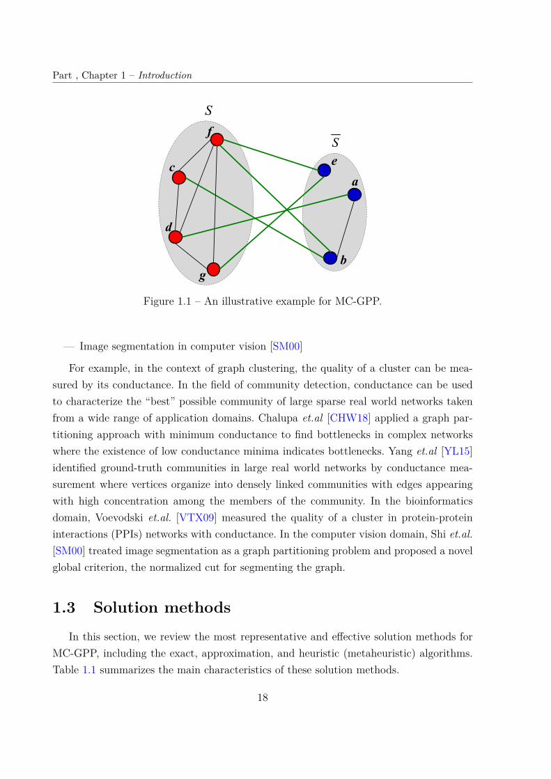
Figure 1.1 shows a graph G = (V,E) with 7 vertices V = a, b, c, d, e, f, g and apartition s = S, S with S = c, d, f, g and S = a, b, e. Since vol(S) = 15, vol(S) = 7and |cut(s)| = 5, the conductance of this partition is Φ(s) = 5/7 = 0.71.
1.2 Applications
From a practical perspective, MC-GPP has a number of practical applications indifferent fields and arises naturally in the context of the real world, including,
— Clustering [Che+06; Sch07; ST13; ZLM13]— Community detection in complex networks [CHW18; For10; Les+08; VM16; YL15]— Bioinformatics [VTX09]
17
Part , Chapter 1 – Introduction
Figure 1.1 – An illustrative example for MC-GPP.
— Image segmentation in computer vision [SM00]
For example, in the context of graph clustering, the quality of a cluster can be mea-sured by its conductance. In the field of community detection, conductance can be usedto characterize the “best” possible community of large sparse real world networks takenfrom a wide range of application domains. Chalupa et.al [CHW18] applied a graph par-titioning approach with minimum conductance to find bottlenecks in complex networkswhere the existence of low conductance minima indicates bottlenecks. Yang et.al [YL15]identified ground-truth communities in large real world networks by conductance mea-surement where vertices organize into densely linked communities with edges appearingwith high concentration among the members of the community. In the bioinformaticsdomain, Voevodski et.al. [VTX09] measured the quality of a cluster in protein-proteininteractions (PPIs) networks with conductance. In the computer vision domain, Shi et.al.[SM00] treated image segmentation as a graph partitioning problem and proposed a novelglobal criterion, the normalized cut for segmenting the graph.
1.3 Solution methods
In this section, we review the most representative and effective solution methods forMC-GPP, including the exact, approximation, and heuristic (metaheuristic) algorithms.Table 1.1 summarizes the main characteristics of these solution methods.
18
1.3. Solution methods
1.3.1 Exact algorithms
Exact methods guarantee the optimality of the found solutions by enumerating, oftenimplicitly, all candidate solutions of the search space. Surprisingly, exact algorithms forthe general MC-GPP were rarely proposed, even if studies exist on special cases.
Hochbaum [Hoc09] devised the first polynomial time algorithms to solve optimallythe ratio region problem and a variant of normalized cut, as well as a few other ratioproblems in the field of image segmentation. These algorithms applied a subroutine ofminimum s, t-cut procedure on a related graph which is of polynomial size and producedthe optimal solution to the respective ratio problems.
Hochbaum [Hoc13] solved a discrete relaxation of a family of NP-hard Rayleigh prob-lems such as the normalized cut problem, the graph expander ratio problem, the Cheegerconstant problem, and the conductance problem. The results showed that the solutionto the discrete Rayleigh ratio problem without balance constraint is strongly polynomialtime solvable, and the algorithm is more efficient and the result is much better than thespectral algorithm.
1.3.2 Approximation algorithms
Approximation methods provide provable performance guarantees on the quality ofthe obtained solutions. Indeed, most existing methods for MC-GPP rely on the approxi-mation framework, and specific to a particular application such as clustering, communityidentification, etc.
Cheeger [Che69] studied the first (and a weak) approximation algorithm for the graphconductance. He established a lower bound for the smallest eigenvalue of the Laplacian,according to a certain global geometric invariant.
Leighton & Rao [LR99] implemented a O(logn)-approximation algorithm for MC-GPP by establishing max-flow min-cut theorems for several classes of multicommodityflow problems.
Arora et al. [AHK04; ARV09] improved Leighton & Rao’s work [LR99] and proposeda O(
√logn)-approximation algorithm for the sparsest cut problem, the edge expansion
problem, the balanced separator problem, and the graph conductance problem. Theyapplied a well-known semidefinite relaxation with triangle inequality constraints to im-plement this algorithm.
Leskovec et al. [Les+09] proposed approximation algorithms for the graph partitioning
19

Part , Chapter 1 – Introduction
problem according to the conductance measure to define and identify clusters or commu-nities in social and information networks. Their results suggest a detailed and counterin-tuitive picture of community structures in large social and information networks.
Spielman et al.[ST13] designed a nearly linear time local clustering algorithm to deter-mine a good cluster, in complying with the conductance measurement. Their clusteringalgorithm can handle massive graphs, such as social networks and web graphs. One ofthe applications of this clustering algorithm can find an approximate sparsest cut with anearly optimal balance.
Zhu et al. [ZLM13] studied random-walk based local algorithms with improved theo-retical guarantees in terms of the clustering accuracy and the conductance. They improvedsignificantly the conductance of cluster where it is well-connected inside.
1.3.3 Heuristic and metaheuristic algorithms
Heuristic and metaheuristic methods aim to find high quality sub-optimal solutions inan acceptable computation time frame, but without provable performance guarantee of thesolutions they found. We observe that solution methods based on modern metaheuristicsremain scarce for MC-GPP, even though they have shown to be powerful tools for solvingmany difficult optimization problems.
Lang & Rao [LR04] proposed the most representative method for MC-GPP, which iscalled the Max-flow Quotient-cut Improvement algorithm (MQI). This method improvesa graph cut when cut quality is measured by quotient-style metrics such as expansion orconductance. Specifically, an initial cut (typically given by the Metis graph partitioningheuristic [KK98b]) by solving the well-known max-flow problem.
Andersen & Lang [AL08] further improved Lang & Rao’s work [LR04] and proposedan algorithm called Improve by solving a sequence of polynomially many s-t minimumcut problems to find a larger-than-expected intersection with lower conductance. Theiralgorithm can prove a stronger guarantee of the lowest conductance, and improve thequality of cuts without impacting the running time.
Lim et al. [Lim+15; Lim+17] proposed a dedicated method called a minus top-kpartition (MTP) for finding a large subgraph with high quality partitions, in terms ofconductance measurement. The results showed that this algorithm can discover a globalbalanced partition with low conductance in real world graphs.
Laarhoven & Marchiori [VM16] studied the continuous optimization of conductancein the context of local network community detection. For their study, they introduced a
20
1.3. Solution methods
new objective function, called σ-conductance, which combines conductance and a regu-larization term controlled by a parameter σ. A projected gradient descent algorithm andan expectation-maximization algorithm were proposed to optimize σ-conductance.
Chalupa [Cha17; CHW18] presented several dedicated heuristic algorithms based onthe general local search and memetic search frameworks to tackle MC-GPP as a pseudo-Boolean optimization problem. They proposed the basic search components for MC-GPPand reported experimental results on real world social networks.
1.3.4 Summary
The literature reviews above indicate that unlike other popular graph partition prob-lems for which numerous solution methods are available (see recent reviews [BH13d;Bul+16]), research on practical solution methods for MC-GPP remains quite limited.There is clearly an urgent need for effective algorithms able to solve large graphs for MC-GPP. Meanwhile, given the NP-hardness of the problem, unless P = NP, exact approacheswill have an exponential time complexity and thus can only be applied to solve probleminstances of limited sizes or instances with particular structures. Indeed, most existingmethods rely on the approximation framework. These methods are either specific to aparticular application (e.g., clustering, community identification) or become unpracticalfor large graphs due to their high computational complexity. One observes that solutionmethods based on modern metaheuristics remain scarce, even though they have shown tobe powerful tools for solving difficult optimization problems. Indeed, heuristic algorithmswere largely neglected and research on such methods is still in its infancy. This thesis thusaims to enrich the toolkit of practical solution methods for MC-GPP by introducing threestate-of-the-art metaheuristic methods as follows. Chapter 2 presents a novel heuristicalgorithm called stagnation aware breakout tabu search (SaBTS) to compute the conduc-tance on small and medium size graphs with up to 500,000 vertices. Chapter 3 introducesa novel hybrid evolutionary algorithm called MAMC to find high quality solutions of lowconductance for large-scale graphs with up to 23 million vertices. Chapter 4 proposes thefirst multilevel optimization algorithm called the iterated multilevel simulated annealingalgorithm (IMSA) for tackling MC-GPP on very large graphs.
21

Part , Chapter 1 – Introduction
Table 1.1 – Summary of the key features and technical contributions of the most relatedstudies for MC-GPP.
Reference Aim Approach Main features Test Limitations
Exact methods
Hochbaum[Hoc09] (2009)
Solve the ratio region problem,a variant of normalized cut inthe field of image segmentation
Max-flow min-cutalgorithm
Exact solution to the givenproblem No Specific or
particularcases; highcomputationalcomplexity;unpractical forlarge graphs
Hochbaum[Hoc13] (2013)
Solve a discrete relaxationof a family of NP-hardRayleigh problems
Max-flow min-cutalgorithm
Solution to the discrete Rayleighratio problem without balanceconstraint in strongly polynomialtime; better solutions thanspectral approach
Yes
Approximation methods
Cheeger[Che69] (1969)
Provide a lower boundfor the smallest eigenvalueof the Laplacian
Mathematicalmethod
Establish a lower boundin terms of a certain globalgeometric invariant
No
Specific orparticularcases; highcomputationalcomplexity
Leighton & Rao[LR99] (1999)
Establish max-flow min-cuttheorems for several classes ofmulticommodity flow problems
Max-flow min-cutalgorithm
Implement a O(logn)-approximation algorithmfor MC-GPP
No
Arora et al.[AHK04; ARV09](2004, 2009)
Propose a O(√logn)-
approximation algorithmfor MC-GPP
Semidefiniteprogramming
Improve a O(logn)-approximation of Leighton &Rao [LR99] (1999)
No
Leskovec et al.[Les+09] (2009)
Define and identifyclusters or communitiesmeasured by conductance
Flow-based,spectral andhierarchical methods
Suggest a detailed andcounterintuitive picture ofcommunity structures in largesocial and information networks
Yes
Spielman et al.[ST13] (2013)
Determine a good clustermeasured by conductance
Nearly linear timelocal clusteringalgorithm
Handle massive graphs; Findan approximate sparsest cutwith nearly optimal balance
Yes
Zhu et al.[ZLM13] (2013)
Find well-connected clustersin terms of the conductance
Random-walk basedlocal algorithms
Improve significantly theconductance of cluster whereit is well-connected inside
Yes
Heuristic and metaheuristic methods
Lang & Rao[LR04] (2004)
Improve a graph cut whencut quality is measured byquotient-style metrics suchas expansion or conductance
Max-flow min-cutalgorithm
Refine the results of Metisgraph partitioning heuristic;Run in nearly linear time
Yes
Decrease ofperformanceon massivegraphs (withmillions ofvertices)
Andersen & Lang[AL08] (2008)
Find a larger-than-expected intersectionwith lower conductance
Sequence andpolynomially manyapplications of max-flowmin-cut algorithm
Prove a stronger guarantee ofthe lowest conductance; Improvethe quality of cuts withoutimpacting the running time
Yes
Lim et al.[Lim+15; Lim+17](2015, 2017)
Find a large subgraphwith high quality partition,in terms of conductance
Remove hub vertices,and find conductanceof a subgraph by graphpartitioning method
Discover a global balancedpartition with low conductancein real world graphs
Yes
Laarhoven &Marchiori[VM16] (2016)
Study continuous optimizationof conductance for localnetwork community detection
Projected gradientdescent and expectation-maximization algorithm
Propose σ-conductance function;Prove locality and performanceguarantees of algorithms
Yes
Chalupa[Cha17] (2017)
Solve MC-GPP as apseudo-Boolean optimizationproblem
Local search andmemetic search
Basic search strategies; appliedto real world social networks Yes
22

1.4. Benchmark instances
1.4 Benchmark instances
To examine the performance of the algorithms presented in this thesis, we conductexperiments on the following benchmarks with a total of 160 instances. The problem in-stances can be divide into four sets as follows, and the detailed characteristics of theseinstances are shown in Table 1.2 to Table 1.4. All of the graphs presented here are undi-rected and connected graphs with unit weight for both the vertices and edges.
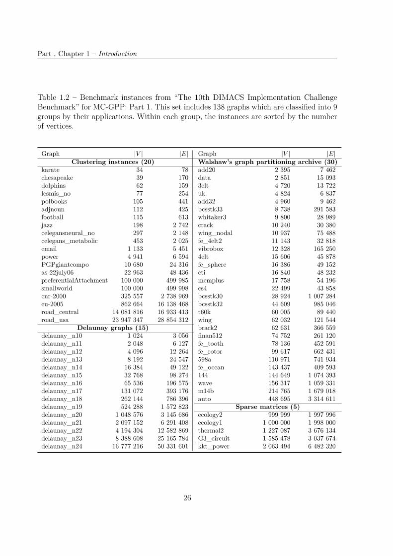
1) The 10th DIMACS Implementation Challenge Benchmark 1. This set con-tains 138 large-size artificial and real world graphs from a wide range of applications,which are dedicated to two related problems of graph partitioning and graph clustering[Bad+14; Bad+13]. Specifically, we use the following 9 popular families:
— Clustering instances (20 graphs). They come from real world applications and oftenused for testing algorithms of graph clustering and community detection.
— Delaunay graphs (15 graphs). They are denoted by DelaunayX, which is generatedas Delaunay triangulations of 2X random points in the unit square [HSS10].
— Walshaw’s graph partitioning archive (30 graphs). They come from real world ap-plications such as finite element computations, matrix computations, VLSI Design,and shortest path computations, which are popular for assessing graph partitioningalgorithms [SWC04].
— Sparse matrices (5 graphs). thermal2 is created from the steady state thermalproblem. ecology2 and ecology1 are generated from the landscape ecology prob-lem. G3_circuit stems from circuit simulation matrices. kkt_power comes from theoptimal power flow, nonlinear optimization (KKT).
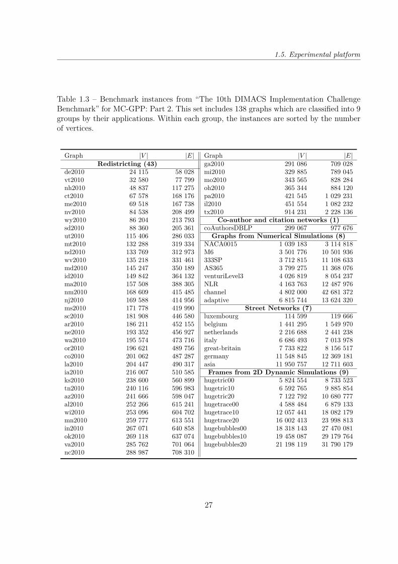
— Redistricting (43 graphs). They represent US states denoted by the XX2010, XXprefix in the filenames are the U.S, e.g. ny is New York. They are popular for solvingthe redistricting and graph partitioning problems.
— Co-author and citation networks (1 graph). They is an example of social networks,which is the popular DBLP website (Digital Bibliography and Library Project).
— Graphs from Numerical Simulations (8 graphs). adaptive and venturiLevel3 originatefrom [Heu10]. channel comes from [WZ11]. 333SP and AS365 are two-dimensional(2D) finite element triangular meshes actually converted from existing 3D models to
1. https://www.cc.gatech.edu/dimacs10/downloads.shtml
23
Part , Chapter 1 – Introduction
2D places, while NACA0015, M6, and NLR are 2D finite element triangular meshescreated from geometry [CLA12].
— Street Networks (7 graphs). They are real world street networks with undirectedand unweighted versions of the largest strongly connected component of the corre-sponding Open Street Map road networks.
— Frames from 2D Dynamic Simulations (9 graphs). They have been created withthe generator described in [MS05]. These graphs are meshes taken from individualframes of a dynamic sequence that resembles 2D adaptive numerical simulations.The files presented here are the frames 0, 10, and 20 of the sequences, respectively.
2) Social networks 2. This set includes 12 anonymized real world social networkgraphs that are extracted from the popular SNAP collection [LK14] and tested in [Cha17].Specifically, soc_52 is a small 52-vertex social network sample, gplus_X are samplesof public circles data from social network Google+, and pokec_X are samples of socialnetwork Pokec. X denotes the number of vertices for each instance.
3) The Network Data Repository online 3. This set involves 10 massive realworld network graphs [RA15] from 5 general collections, including collaboration networks,infrastructure networks, scientific computing, social networks, and web graphs.
4) The complex real-world networks 4. We test the approach proposed in Chap-ter 3 for community detection on 3 popular complex real world networks: Zachary’sKarate Club, College Football Network, and Bottlenose Dolphin Social Network. Thesethree graphs can be also found in the DIMACS10 set.
1.5 Experimental platform
All the proposed algorithms in this thesis were implemented in C++ and compiled us-ing the g++ compiler with the “-O3” option. The experiment in Chapter 2 was conductedon an Intel Xeon E5440 processor (2.83GHz) with 2GB RAM under Linux operating sys-tem. The experiments in Chapter 3 and Chapter 4 were conducted on an AMD Opteron4184 processor (2.80GHz) with 32GB RAM under Linux operating system.
The source codes of all the presented algorithms in this thesis are publicly availableonline and listed as follows,
2. http://davidchalupa.github.io/research/data/social.html3. http://networkrepository.com/index.php4. http://www-personal.umich.edu/~mejn/netdata/
24

1.5. Experimental platform
— In Chapter 2, the proposed SaBTS algorithm is available at: http://www.info.univ-angers.fr/~hao/mcgpp.html.
— In Chapter 3, the proposed MAMC algorithm is available at: http://www.info.univ-angers.fr/~hao/mamc.html.
— In Chapter 4, the proposed IMSA algorithm is available at: http://www.info.univ-angers.fr/pub/hao/IMSA.html
25
Part , Chapter 1 – Introduction
Table 1.2 – Benchmark instances from “The 10th DIMACS Implementation ChallengeBenchmark” for MC-GPP: Part 1. This set includes 138 graphs which are classified into 9groups by their applications. Within each group, the instances are sorted by the numberof vertices.
Graph |V | |E| Graph |V | |E|Clustering instances (20) Walshaw’s graph partitioning archive (30)
karate 34 78 add20 2 395 7 462chesapeake 39 170 data 2 851 15 093dolphins 62 159 3elt 4 720 13 722lesmis_no 77 254 uk 4 824 6 837polbooks 105 441 add32 4 960 9 462adjnoun 112 425 bcsstk33 8 738 291 583football 115 613 whitaker3 9 800 28 989jazz 198 2 742 crack 10 240 30 380celegansneural_no 297 2 148 wing_nodal 10 937 75 488celegans_metabolic 453 2 025 fe_4elt2 11 143 32 818email 1 133 5 451 vibrobox 12 328 165 250power 4 941 6 594 4elt 15 606 45 878PGPgiantcompo 10 680 24 316 fe_sphere 16 386 49 152as-22july06 22 963 48 436 cti 16 840 48 232preferentialAttachment 100 000 499 985 memplus 17 758 54 196smallworld 100 000 499 998 cs4 22 499 43 858cnr-2000 325 557 2 738 969 bcsstk30 28 924 1 007 284eu-2005 862 664 16 138 468 bcsstk32 44 609 985 046road_central 14 081 816 16 933 413 t60k 60 005 89 440road_usa 23 947 347 28 854 312 wing 62 032 121 544
Delaunay graphs (15) brack2 62 631 366 559delaunay_n10 1 024 3 056 finan512 74 752 261 120delaunay_n11 2 048 6 127 fe_tooth 78 136 452 591delaunay_n12 4 096 12 264 fe_rotor 99 617 662 431delaunay_n13 8 192 24 547 598a 110 971 741 934delaunay_n14 16 384 49 122 fe_ocean 143 437 409 593delaunay_n15 32 768 98 274 144 144 649 1 074 393delaunay_n16 65 536 196 575 wave 156 317 1 059 331delaunay_n17 131 072 393 176 m14b 214 765 1 679 018delaunay_n18 262 144 786 396 auto 448 695 3 314 611delaunay_n19 524 288 1 572 823 Sparse matrices (5)delaunay_n20 1 048 576 3 145 686 ecology2 999 999 1 997 996delaunay_n21 2 097 152 6 291 408 ecology1 1 000 000 1 998 000delaunay_n22 4 194 304 12 582 869 thermal2 1 227 087 3 676 134delaunay_n23 8 388 608 25 165 784 G3_circuit 1 585 478 3 037 674delaunay_n24 16 777 216 50 331 601 kkt_power 2 063 494 6 482 320
26
1.5. Experimental platform
Table 1.3 – Benchmark instances from “The 10th DIMACS Implementation ChallengeBenchmark” for MC-GPP: Part 2. This set includes 138 graphs which are classified into 9groups by their applications. Within each group, the instances are sorted by the numberof vertices.
Graph |V | |E| Graph |V | |E|Redistricting (43) ga2010 291 086 709 028
de2010 24 115 58 028 mi2010 329 885 789 045vt2010 32 580 77 799 mo2010 343 565 828 284nh2010 48 837 117 275 oh2010 365 344 884 120ct2010 67 578 168 176 pa2010 421 545 1 029 231me2010 69 518 167 738 il2010 451 554 1 082 232nv2010 84 538 208 499 tx2010 914 231 2 228 136wy2010 86 204 213 793 Co-author and citation networks (1)sd2010 88 360 205 361 coAuthorsDBLP 299 067 977 676ut2010 115 406 286 033 Graphs from Numerical Simulations (8)mt2010 132 288 319 334 NACA0015 1 039 183 3 114 818nd2010 133 769 312 973 M6 3 501 776 10 501 936wv2010 135 218 331 461 333SP 3 712 815 11 108 633md2010 145 247 350 189 AS365 3 799 275 11 368 076id2010 149 842 364 132 venturiLevel3 4 026 819 8 054 237ma2010 157 508 388 305 NLR 4 163 763 12 487 976nm2010 168 609 415 485 channel 4 802 000 42 681 372nj2010 169 588 414 956 adaptive 6 815 744 13 624 320ms2010 171 778 419 990 Street Networks (7)sc2010 181 908 446 580 luxembourg 114 599 119 666ar2010 186 211 452 155 belgium 1 441 295 1 549 970ne2010 193 352 456 927 netherlands 2 216 688 2 441 238wa2010 195 574 473 716 italy 6 686 493 7 013 978or2010 196 621 489 756 great-britain 7 733 822 8 156 517co2010 201 062 487 287 germany 11 548 845 12 369 181la2010 204 447 490 317 asia 11 950 757 12 711 603ia2010 216 007 510 585 Frames from 2D Dynamic Simulations (9)ks2010 238 600 560 899 hugetric00 5 824 554 8 733 523tn2010 240 116 596 983 hugetric10 6 592 765 9 885 854az2010 241 666 598 047 hugetric20 7 122 792 10 680 777al2010 252 266 615 241 hugetrace00 4 588 484 6 879 133wi2010 253 096 604 702 hugetrace10 12 057 441 18 082 179mn2010 259 777 613 551 hugetrace20 16 002 413 23 998 813in2010 267 071 640 858 hugebubbles00 18 318 143 27 470 081ok2010 269 118 637 074 hugebubbles10 19 458 087 29 179 764va2010 285 762 701 064 hugebubbles20 21 198 119 31 790 179nc2010 288 987 708 310
27
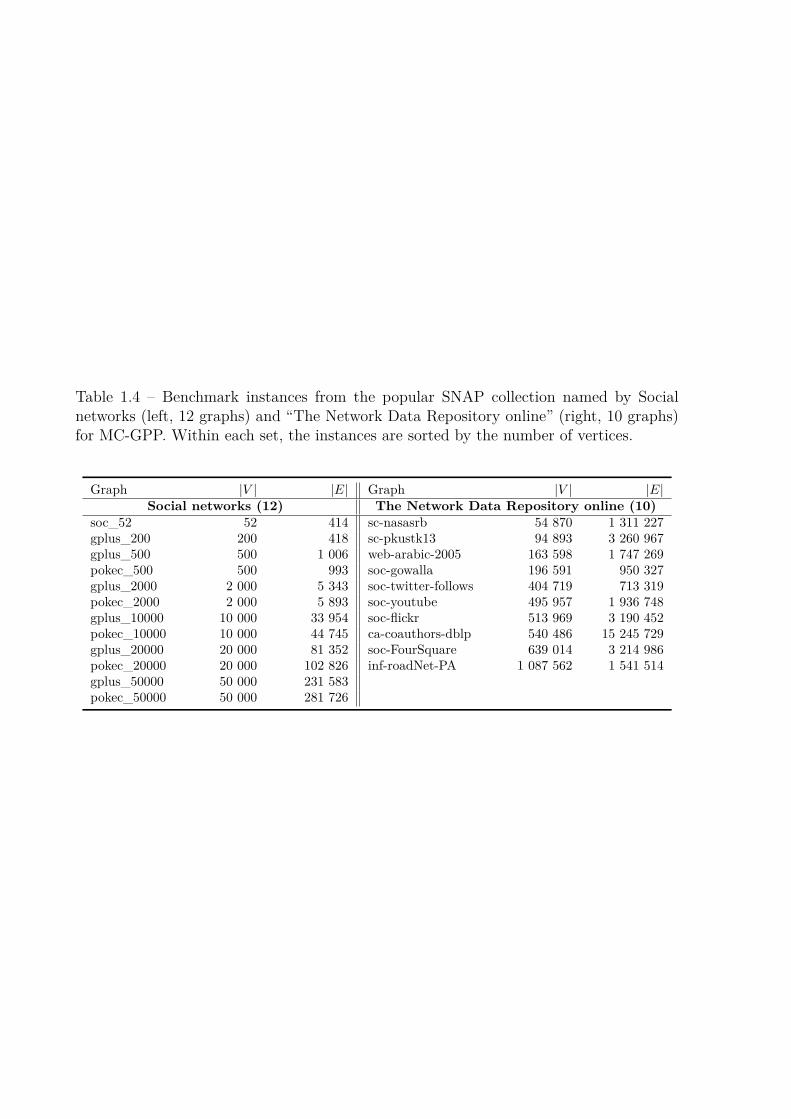
Table 1.4 – Benchmark instances from the popular SNAP collection named by Socialnetworks (left, 12 graphs) and “The Network Data Repository online” (right, 10 graphs)for MC-GPP. Within each set, the instances are sorted by the number of vertices.
Graph |V | |E| Graph |V | |E|Social networks (12) The Network Data Repository online (10)
soc_52 52 414 sc-nasasrb 54 870 1 311 227gplus_200 200 418 sc-pkustk13 94 893 3 260 967gplus_500 500 1 006 web-arabic-2005 163 598 1 747 269pokec_500 500 993 soc-gowalla 196 591 950 327gplus_2000 2 000 5 343 soc-twitter-follows 404 719 713 319pokec_2000 2 000 5 893 soc-youtube 495 957 1 936 748gplus_10000 10 000 33 954 soc-flickr 513 969 3 190 452pokec_10000 10 000 44 745 ca-coauthors-dblp 540 486 15 245 729gplus_20000 20 000 81 352 soc-FourSquare 639 014 3 214 986pokec_20000 20 000 102 826 inf-roadNet-PA 1 087 562 1 541 514gplus_50000 50 000 231 583pokec_50000 50 000 281 726
Chapter 2
SABTS: STAGNATION-AWARE
BREAKOUT TABU SEARCH FOR THE
MINIMUM CONDUCTANCE GRAPH
PARTITIONING PROBLEM
2.1 Introduction
In this chapter, we focus our research on effective heuristic search for MC-GPP that canbe used to find high quality solutions for problem instances that cannot be solved exactly.Precisely, we develop a novel heuristic algorithm called Stagnation-aware Breakout TabuSearch (SaBTS) to compute the conductance of a general graph. We summarize the maincontributions as follows.
— The proposed SaBTS algorithm adapts for the first time the general breakout localsearch method [BH13a; BH13b; BH13c] to MC-GPP. SaBTS integrates a dedicatedtabu search procedure with a constrained neighborhood to find high quality solu-tions and a self-adaptive and multi-strategy perturbation mechanism to escape localoptimum traps.
— We demonstrate the effectiveness of the proposed SaBTS algorithm on 110 bench-mark instances including 98 graphs from the 10th DIMACS Implementation Chal-lenge Benchmark and 12 anonymized social networks. The computational studiesindicate that SaBTS dominates a recent dedicated algorithm (StS-AMA) [Cha17;CHW18]. Moreover, when SaBTS is run as a post-processing method, it consis-tently improves on the solutions provided by the popular graph partitioning toolMetis [KK98b] and the state-of-the-art max-flow-based method MQI [LR04]. Toshed light on the understanding of the algorithm, we study the impacts of its key
29

Part , Chapter 2 – SaBTS: Stagnation-aware breakout tabu search for the minimumconductance graph partitioning problem
algorithmic components.
The chapter is organized as follows. Section 2.2 describes the general scheme of theproposed SaBTS algorithm and its algorithmic components. Section 2.3 is dedicated tocomputational results and comparisons. Section 2.4 investigates several key algorithmiccomponents to understand their impact on the performance of the proposed SaBTS algo-rithm. We draw conclusions in the last section.
2.2 Stagnation-aware breakout tabu search for MC-GPP
In this section, we present the proposed heuristic algorithm for tackling MC-GPP. Wefirst introduce the general procedure and then explain the composing ingredients.
2.2.1 Main scheme
The proposed stagnation-aware breakout tabu search algorithm (SaBTS) for MC-GPPadopts the general breakout local search method (BLS) introduced in [BH13a; BH13b;BH13c]. BLS relies on a dedicated local search procedure to find local optimal solutionsand an adaptive perturbation procedure to jump out of local optimum traps. In addition tothe local search procedure which ensures search intensification, BLS employs its adaptiveperturbation mechanism to reach a suitable search diversification. This is achieved bydynamically determining the number of perturbation moves (i.e., the jump magnitude)and the type of perturbation (with different intensities). By iterating the local searchphase and the adaptive perturbation phase, the method favors a balanced search in termsof intensification and diversification and helps to find high-quality solutions in the givensearch space.
From a perspective of algorithm design, the proposed SaBTS algorithm is composedof two principal components: a constrained neighborhood tabu search procedure (CNTS,Section 2.2.3) and a self-adaptive perturbation procedure (SAP, Section 2.2.4). Startingwith an initial solution that can be provided by any means (Section 2.2.2), SaBTS usesthe CNTS procedure to perform an intensified examination of candidate solutions to findimproved solutions. Upon the termination of the CNTS procedure, SaBTS triggers theSAP procedure to diversify the search and drive the process to new and unexplored zones.SaBTS iterates these two procedures to discover solutions of increasing quality.
30
2.2. Stagnation-aware breakout tabu search for MC-GPP
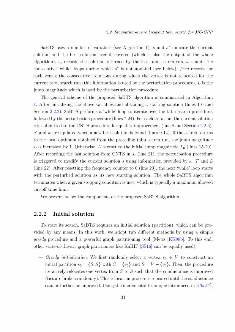
SaBTS uses a number of variables (see Algorithm 1): s and s∗ indicate the currentsolution and the best solution ever discovered (which is also the output of the wholealgorithm), st records the solution returned by the last tabu search run, ω counts theconsecutive ‘while’ loops during which s∗ is not updated (see below), freq records foreach vertex the consecutive iterations during which the vertex is not relocated for thecurrent tabu search run (this information is used by the perturbation procedure), L is thejump magnitude which is used by the perturbation procedure.
The general scheme of the proposed SaBTS algorithm is summarized in Algorithm1. After initializing the above variables and obtaining a starting solution (lines 1-6 andSection 2.2.2), SaBTS performs a ‘while’ loop to iterate over the tabu search procedure,followed by the perturbation procedure (lines 7-24). For each iteration, the current solutions is submitted to the CNTS procedure for quality improvement (line 8 and Section 2.2.3).s∗ and w are updated when a new best solution is found (lines 9-14). If the search returnsto the local optimum obtained from the preceding tabu search run, the jump magnitudeL is increased by 1. Otherwise, L is reset to the initial jump magnitude L0 (lines 15-20).After recording the last solution from CNTS in st (line 21), the perturbation procedureis triggered to modify the current solution s using information provided by ω, T and L(line 22). After resetting the frequency counter to 0 (line 23), the next ‘while’ loop startswith the perturbed solution as its new starting solution. The whole SaBTS algorithmterminates when a given stopping condition is met, which is typically a maximum allowedcut-off time limit.
We present below the components of the proposed SaBTS algorithm.
2.2.2 Initial solution
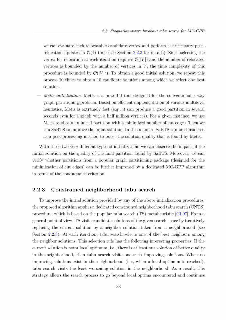
To start its search, SaBTS requires an initial solution (partition), which can be pro-vided by any means. In this work, we adopt two different methods by using a simplegreedy procedure and a powerful graph partitioning tool (Metis [KK98b]. To this end,other state-of-the-art graph partitioners like KaHIP [SS16] can be equally used).
— Greedy initialization. We first randomly select a vertex v0 ∈ V to construct aninitial partition s0 = S, S with S = v0 and S = V − v0. Then, the procedureiteratively relocates one vertex from S to S such that the conductance is improved(ties are broken randomly). This relocation process is repeated until the conductancecannot further be improved. Using the incremental technique introduced in [Cha17],
31

Part , Chapter 2 – SaBTS: Stagnation-aware breakout tabu search for the minimumconductance graph partitioning problem
Algorithm 1 Main framework of the stagnation-aware breakout tabu search (SaBTS)for MC-GPP.Require: Graph G = (V,E), depth of tabu search D, stagnation threshold T , initial jumpmagnitude L0.Ensure: The best partition s∗ found so far.1: ω ← 0 /∗ initialize counter of non-improving local optima ∗/2: freq(v)← 0 for all v ∈ V /∗ initialize move frequency of vertices, Section 2.2.3 ∗/3: L← L0 /∗ initialize jump magnitude, Section 2.2.4 ∗/4: s← Initial_Solution_Generation() /∗ Section 2.2.2 ∗/5: st ← s /∗ record the last local optimum found ∗/6: s∗ ← s /∗ the best solution encountered until now ∗/7: while Stopping condition is not satisfied do8: s← Constrained_Neighborhood_Tabu_Search(s,D, freq) /∗ Section 2.2.3 ∗/9: if Φ(s) < Φ(s∗) then10: s∗ ← s /∗ update the best solution found so far ∗/11: ω ← 012: else13: ω ← ω + 114: end if15: /∗ search returns to last local optimum, increase jump magnitude L ∗/16: if s = st then17: L← L+ 118: else19: L = L020: end if21: st ← s /∗ record the current solution, to be used in line 16 of next loop ∗/22: s← Self_Adaptive_Perturbation(s, ω, T, L, freq) /∗ Section 2.2.4 ∗/23: freq(v)← 0 for all v ∈ V /∗ reset move frequency of vertices ∗/24: end while25: return s∗
32
2.2. Stagnation-aware breakout tabu search for MC-GPP
we can evaluate each relocatable candidate vertex and perform the necessary post-relocation updates in O(1) time (see Section 2.2.3 for details). Since selecting thevertex for relocation at each iteration requires O(|V |) and the number of relocatedvertices is bounded by the number of vertices in V , the time complexity of thisprocedure is bounded by O(|V |2). To obtain a good initial solution, we repeat thisprocess 10 times to obtain 10 candidate solutions among which we select one bestsolution.
— Metis initialization. Metis is a powerful tool designed for the conventional k-waygraph partitioning problem. Based on efficient implementation of various multilevelheuristics, Metis is extremely fast (e.g., it can produce a good partition in severalseconds even for a graph with a half million vertices). For a given instance, we useMetis to obtain an initial partition with a minimized number of cut edges. Then werun SaBTS to improve the input solution. In this manner, SaBTS can be consideredas a post-processing method to boost the solution quality that is found by Metis.
With these two very different types of initialization, we can observe the impact of theinitial solution on the quality of the final partition found by SaBTS. Moreover, we canverify whether partitions from a popular graph partitioning package (designed for theminimization of cut edges) can be further improved by a dedicated MC-GPP algorithmin terms of the conductance criterion.
2.2.3 Constrained neighborhood tabu search
To improve the initial solution provided by any of the above initialization procedures,the proposed algorithm applies a dedicated constrained neighborhood tabu search (CNTS)procedure, which is based on the popular tabu search (TS) metaheuristic [GL97]. From ageneral point of view, TS visits candidate solutions of the given search space by iterativelyreplacing the current solution by a neighbor solution taken from a neighborhood (seeSection 2.2.3). At each iteration, tabu search selects one of the best neighbors amongthe neighbor solutions. This selection rule has the following interesting properties. If thecurrent solution is not a local optimum, i.e., there is at least one solution of better qualityin the neighborhood, then tabu search visits one such improving solutions. When noimproving solutions exist in the neighborhood (i.e., when a local optimum is reached),tabu search visits the least worsening solution in the neighborhood. As a result, thisstrategy allows the search process to go beyond local optima encountered and continues
33
Part , Chapter 2 – SaBTS: Stagnation-aware breakout tabu search for the minimumconductance graph partitioning problem
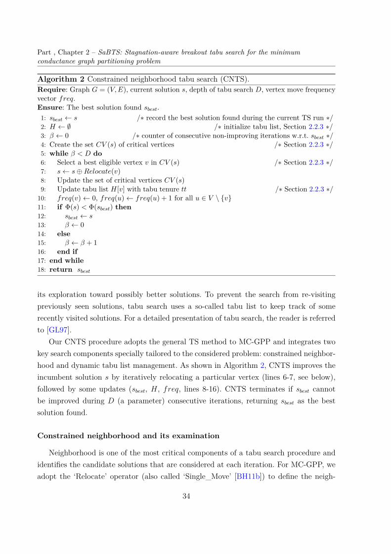
Algorithm 2 Constrained neighborhood tabu search (CNTS).Require: Graph G = (V,E), current solution s, depth of tabu search D, vertex move frequencyvector freq.Ensure: The best solution found sbest.1: sbest ← s /∗ record the best solution found during the current TS run ∗/2: H ← ∅ /∗ initialize tabu list, Section 2.2.3 ∗/3: β ← 0 /∗ counter of consecutive non-improving iterations w.r.t. sbest ∗/4: Create the set CV (s) of critical vertices /∗ Section 2.2.3 ∗/5: while β < D do6: Select a best eligible vertex v in CV (s) /∗ Section 2.2.3 ∗/7: s← s⊕Relocate(v)8: Update the set of critical vertices CV (s)9: Update tabu list H[v] with tabu tenure tt /∗ Section 2.2.3 ∗/10: freq(v)← 0, freq(u)← freq(u) + 1 for all u ∈ V \ v11: if Φ(s) < Φ(sbest) then12: sbest ← s13: β ← 014: else15: β ← β + 116: end if17: end while18: return sbest
its exploration toward possibly better solutions. To prevent the search from re-visitingpreviously seen solutions, tabu search uses a so-called tabu list to keep track of somerecently visited solutions. For a detailed presentation of tabu search, the reader is referredto [GL97].
Our CNTS procedure adopts the general TS method to MC-GPP and integrates twokey search components specially tailored to the considered problem: constrained neighbor-hood and dynamic tabu list management. As shown in Algorithm 2, CNTS improves theincumbent solution s by iteratively relocating a particular vertex (lines 6-7, see below),followed by some updates (sbest, H, freq, lines 8-16). CNTS terminates if sbest cannotbe improved during D (a parameter) consecutive iterations, returning sbest as the bestsolution found.
Constrained neighborhood and its examination
Neighborhood is one of the most critical components of a tabu search procedure andidentifies the candidate solutions that are considered at each iteration. For MC-GPP, weadopt the ‘Relocate’ operator (also called ‘Single_Move’ [BH11b]) to define the neigh-
34
2.2. Stagnation-aware breakout tabu search for MC-GPP
borhood. Basically, let s = S, S be the incumbent solution, the ‘Relocate’ operatordisplaces a vertex from its current set S or S to the complement set. Let v be the vertexto be displaced. We use s′ = s⊕Relocate(v) to denote the neighbor solution s′ obtainedby relocating v. Then the classic neighborhood induced by the ‘Relocate’ operator, isgiven by:
N (s) = s′ : s⊕Relocate(v), v ∈ S or v ∈ S (2.1)
One notices that this neighborhood is unconstrained in the sense that every vertex of Vis a possible candidate for the ‘Relocate’ operator. However, the size of this neighborhoodis in order O(|V |), implying that its exploration would be time-consuming and expensivein particular for large graphs. Meanwhile, we observe that this unconstrained neighbor-hood includes many non-promising neighbor solutions that are irrelevant for conductanceimprovement as discussed below.
For these reasons, we introduce a constrained neighborhood that focuses on promisingneighbor solutions and is of smaller size. The rationale behind the constrained neighbor-hood is that in terms of conductance improvement, all vertices are not equally interestingfor the ‘Relocate’ operator. The idea is then to identify the “critical” vertices that arerelevant for the ‘Relocate’ operator and exclude the “non-critical” vertices (or “ordinary”vertices) for consideration.
Given a solution s = S, S, let e(S) = |(u, v) ⊂ E : u, v ∈ S| and e(S) =|(u, v) ⊂ E : u, v ∈ S| be the number of edges whose endpoints belong to S and S
respectively. Then, it is easy to check that the volume of sets S and S can be re-writtenas: vol(S) = 2e(S) + |cut(s)|, vol(S) = 2e(S) + |cut(s)|. Thus, the conductance Φ(s) canbe re-expressed as follows,
Φ(s) = |cut(s)|minvol(S), vol(S)
= |cut(s)||cut(s)|+ 2 ·mine(S), e(S)
= 1/
1 + 2 · mine(S), e(S)|cut(s)|
(2.2)
By equation (2.2), it is clear that increasingmine(S), e(S) and decreasing |cut(s)| re-duces the conductance Φ(s). Inversely, decreasing mine(S), e(S) and increasing |cut(s)|augment the conductance Φ(s).
Let CV (s) = v ∈ V : (v,_) ∈ cut(s) be the set of critical vertices of s, i.e., the
35
Part , Chapter 2 – SaBTS: Stagnation-aware breakout tabu search for the minimumconductance graph partitioning problem
dj
f
e
b
a
c
g
i
h
S
S
S
dj
f
eb
a
c
g
i
hl
k
S
CASE 1: e(S) = e( )S = a, b, c, d, = e, f, g, h, i, j, ϕ(s) = 0.23.Move from S to , ϕ(s') = 0.45↑.
SS
)(sOVa S
CASE 2: e(S) ≠ e( ), S = a, b, c, d, k, l, = e, f, g, h, i, j, ϕ(s) = 0.23.(1) Move from large set S to small set
Move , ϕ(s') = 0.45↑.(2) Move from small set to large set S
Move ( ), ϕ(s') = 0.38↑.Move ( ), ϕ(s') = 0.31↑. Move ( ), ϕ(s') = 0.47↑.
S
)(sOVg
)deg(k)deg( l)deg(c
3S
)(sOVk)(sOVl)(sOVc
S
S
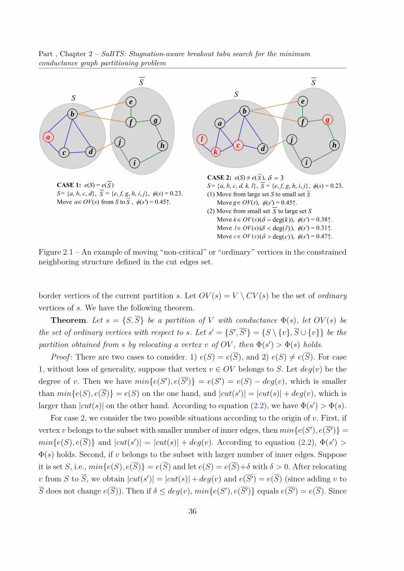
Figure 2.1 – An example of moving “non-critical” or “ordinary” vertices in the constrainedneighboring structure defined in the cut edges set.
border vertices of the current partition s. Let OV (s) = V \ CV (s) be the set of ordinaryvertices of s. We have the following theorem.
Theorem. Let s = S, S be a partition of V with conductance Φ(s), let OV (s) bethe set of ordinary vertices with respect to s. Let s′ = S ′, S ′ = S \ v, S ∪ v be thepartition obtained from s by relocating a vertex v of OV , then Φ(s′) > Φ(s) holds.
Proof : There are two cases to consider. 1) e(S) = e(S), and 2) e(S) 6= e(S). For case1, without loss of generality, suppose that vertex v ∈ OV belongs to S. Let deg(v) be thedegree of v. Then we have mine(S ′), e(S ′) = e(S ′) = e(S) − deg(v), which is smallerthan mine(S), e(S) = e(S) on the one hand, and |cut(s′)| = |cut(s)|+ deg(v), which islarger than |cut(s)| on the other hand. According to equation (2.2), we have Φ(s′) > Φ(s).
For case 2, we consider the two possible situations according to the origin of v. First, ifvertex v belongs to the subset with smaller number of inner edges, thenmine(S ′), e(S ′) =mine(S), e(S) and |cut(s′)| = |cut(s)| + deg(v). According to equation (2.2), Φ(s′) >Φ(s) holds. Second, if v belongs to the subset with larger number of inner edges. Supposeit is set S, i.e.,mine(S), e(S) = e(S) and let e(S) = e(S)+δ with δ > 0. After relocatingv from S to S, we obtain |cut(s′)| = |cut(s)|+ deg(v) and e(S ′) = e(S) (since adding v toS does not change e(S)). Then if δ ≤ deg(v), mine(S ′), e(S ′) equals e(S ′) = e(S). Since
36
2.2. Stagnation-aware breakout tabu search for MC-GPP
|cut(s′)| = |cut(s)|+ deg(v) > |cut(s)|, we have Φ(s′) > Φ(s) according to equation (2.2).Otherwise, if δ > deg(v), mine(S ′), e(S ′) = e(S ′) = e(S) − deg(v). Since e(S ′) < e(S)and |cut(s′)| > |cut(s)|, we have again Φ(s′) > Φ(s) according to equation (2.2). Thisfinishes the proof of the theorem.
This theorem indicates that ordinary vertices are not interesting for the ‘Relocate’operator since they always deteriorate the conductance of the current solution (see Figure2.1 for an example). Consequently, it is relevant to exclude these ordinary vertices andonly consider the critical vertices of set CV (s). This consideration leads to our criticalvertices constrained neighborhood NC ,
NC(s) = s′ : s⊕Relocate(v), v ∈ CV (s) (2.3)
Compared to the unconstrained neighborhood N (s) whose size is of O(|V |) (see Equa-tion (2.1)), the constrained neighborhood NC(s) has a size of O(|CV (s)|). The experi-ments suggest that CV (s) is generally much smaller than V (except for very dense graphs).Therefore using NC(s) rather than N (s) is more time-efficient and favors conductance im-provement as well.
To quantify the quality of a neighbor solution s′ obtained by relocating vertex v, weuse δ(v) to denote the move gain as follows.
δ(v) = Φ(s′)− Φ(s) (2.4)
So a negative, zero, and positive δ(v) value indicate an improving, stagnating, andworsening neighbor solution respectively.
To explore the constrained neighborhood NC(s), the CNTS procedure first identifiesthe set CV (s) of critical vertices (Algorithm 2, line 4). This can be achieved in O(|V | ×degmax) time where degmax is the maximum degree of a given graph. Then CNTS performseach subsequent iteration in three steps: 1) selects, among the eligible critical vertices, onebest vertex v (ties are broken randomly) with the smallest move gain, 2) relocate v toobtain a neighbor solution, and 3) make necessary updates.
A vertex qualifies as eligible if it is not forbidden by the tabu list (see Section 2.2.3).Note that if relocating a vertex leads to a solution better than the best solution sbest
found during the tabu search process, this vertex always qualifies as eligible even if it isforbidden by the tabu list (this is called the aspiration criterion in the tabu search).
To ensure the computation efficiency of the CNTS procedure, we adopt the incremental
37
Part , Chapter 2 – SaBTS: Stagnation-aware breakout tabu search for the minimumconductance graph partitioning problem
updating technique [Cha17] to perform the necessary calculations of each CNTS iteration.Given the incumbent solution s = S, S, the number of cut edges |cut(s)|, the degreesof each vertex v in both partition subsets degS(v) and degS(v), let s′ = S ′, S ′ withS ′ = S \ v, S ′ = S ∪ v be the new neighbor solution after relocating v from S to S.The conductance of s′ can be efficiently recalculated in O(1) time,
vol(S ′) = vol(S)− deg(v) (2.5)
vol(S ′) = vol(S) + deg(v) (2.6)
|cut(s′)| = |cut(s)|+ degS(v)− degS(v) (2.7)
After relocating v, we update the auxiliary degrees of each vertex w adjacent to v inO(1) time,
degS′(w) = degS(w)− 1 (2.8)
degS′(w) = degS(w) + 1 (2.9)
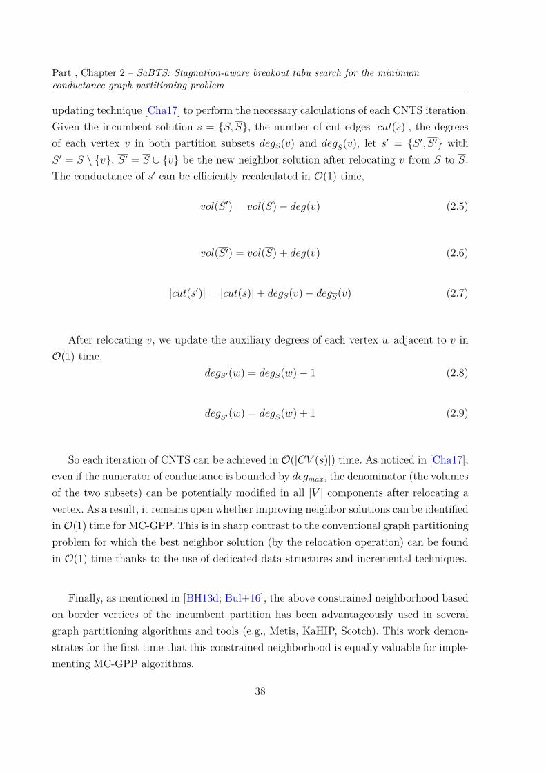
So each iteration of CNTS can be achieved in O(|CV (s)|) time. As noticed in [Cha17],even if the numerator of conductance is bounded by degmax, the denominator (the volumesof the two subsets) can be potentially modified in all |V | components after relocating avertex. As a result, it remains open whether improving neighbor solutions can be identifiedin O(1) time for MC-GPP. This is in sharp contrast to the conventional graph partitioningproblem for which the best neighbor solution (by the relocation operation) can be foundin O(1) time thanks to the use of dedicated data structures and incremental techniques.
Finally, as mentioned in [BH13d; Bul+16], the above constrained neighborhood basedon border vertices of the incumbent partition has been advantageously used in severalgraph partitioning algorithms and tools (e.g., Metis, KaHIP, Scotch). This work demon-strates for the first time that this constrained neighborhood is equally valuable for imple-menting MC-GPP algorithms.
38

2.2. Stagnation-aware breakout tabu search for MC-GPP
Dynamic tabu tenure management
As mentioned above, the CNTS procedure uses a tabu list H to record recently relo-cated vertices to prevent them from being reconsidered for a future relocation and thusavoid revisiting previously visited solutions. Specifically, each time a vertex v ∈ CV isrelocated, v is added in the tabu list and is not considered for next tt(v) iterations (tt iscalled tabu tenure). To implement the tabu list efficiently, we use a vector H of size |V |(initialized to 0) to represent the tabu list. When a vertex v is relocated, H[v] is updatedto iter + tt where iter represents the current number of iterations. Then during the nextiterations, if iter < H[v], v is forbidden by the tabu list; Otherwise, v is not prohibitedby the tabu list.
To determine the tabu tenure tt, we adopt a technique which dynamically adjusts thetabu tenure with a periodic step function F defined over the current iteration number iter[GBF11; WH13]. Typically, each period of the step function consists of 1500 iterations thatare divided into 15 steps (also called intervals) [xi, xi+1 − 1]i=1,2,...,15 with x1 = 1, xi+1 =xi+100. According to the current iteration number, the tabu tenure changes dynamicallyduring the search with one of four possible values: (10×α, 20×α, 40×α, 80×α), where α is aparameter. Precisely, for an iteration iter ∈ [xi, xi+1−1], the tabu tenure tt equals F (iter),which is given by (yi)i=1,2,...,15 = α × (10, 20, 10, 40, 10, 20, 10, 80, 10, 20, 10, 40, 10, 20, 10).The tabu tenure is thus equal to 10×α for the first 100 iterations [1, 100]; then 20×α foriterations from [101, 200]; followed by 10×α again for iterations [201, 300]; and 40×α foriterations [401, 500] etc. After reaching the largest value 80 × α for iterations [701, 800],the tabu tenure drops again to 10× α for the next 100 iterations and so on (see Section2.2.3 of [WH13] for an illustrative example). This dynamic tabu tenure technique has pre-viously shown its usefulness for graph partitioning and max-bisection algorithms [GBF11;WH13]. The experimental study also indicates that this technique is quite suitable forSaBTS as well and helps the algorithm to escape various local optima. Contrary to statictabu tenure techniques, varying the tabu tenure periodically and dynamically makes thealgorithm quite robust across the tested instances and avoids the difficulties encounteredwith manually tuned static techniques.
2.2.4 Self-adaptive perturbation strategy
The tabu search procedure presented in Section 2.2.3 can overcome some local optimumtraps thanks to its tabu list. However, CNTS can still be trapped in deep local optima. To
39
Part , Chapter 2 – SaBTS: Stagnation-aware breakout tabu search for the minimumconductance graph partitioning problem
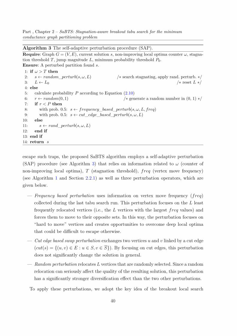
Algorithm 3 The self-adaptive perturbation procedure (SAP).Require: Graph G = (V,E), current solution s, non-improving local optima counter ω, stagna-tion threshold T , jump magnitude L, minimum probability threshold P0.Ensure: A perturbed partition found s.1: if ω > T then2: s← random_perturb(s, ω, L) /∗ search stagnating, apply rand. perturb. ∗/3: L← L0 /∗ reset L ∗/4: else5: calculate probability P according to Equation (2.10)6: r ← random(0, 1) /∗ generate a random number in (0, 1) ∗/7: if r < P then8: with prob. 0.5: s← frequency_based_perturb(s, ω, L, freq)9: with prob. 0.5: s← cut_edge_based_perturb(s, ω, L)10: else11: s ← rand_perturb(s, ω, L)12: end if13: end if14: return s
escape such traps, the proposed SaBTS algorithm employs a self-adaptive perturbation(SAP) procedure (see Algorithm 3) that relies on information related to ω (counter ofnon-improving local optima), T (stagnation threshold), freq (vertex move frequency)(see Algorithm 1 and Section 2.2.1) as well as three perturbation operators, which aregiven below.
— Frequency based perturbation uses information on vertex move frequency (freq)collected during the last tabu search run. This perturbation focuses on the L leastfrequently relocated vertices (i.e., the L vertices with the largest freq values) andforces them to move to their opposite sets. In this way, the perturbation focuses on“hard to move” vertices and creates opportunities to overcome deep local optimathat could be difficult to escape otherwise.
— Cut edge based swap perturbation exchanges two vertices u and v linked by a cut edge(cut(s) = (u, v) ∈ E : u ∈ S, v ∈ S). By focusing on cut edges, this perturbationdoes not significantly change the solution in general.
— Random perturbation relocates L vertices that are randomly selected. Since a randomrelocation can seriously affect the quality of the resulting solution, this perturbationhas a significantly stronger diversification effect than the two other perturbations.
To apply these perturbations, we adopt the key idea of the breakout local search
40
2.3. Experimental results
method [BH13a; BH13b; BH13c] that applies perturbations of different intensity adap-tively and probabilistically. Specifically, if ω > T (i.e., at least T consecutive local optimahave been visited without improving the best solution found s∗, see Algorithm 1), thesearch is believed to be stagnating in a deep local optimum attractor (line 2, Algorithm3). To escape the trap, we apply the random perturbation to change the incumbent so-lution significantly and displace the search to a distant search zone. Otherwise, we applythe three perturbations in a probabilistic way. For this purpose, we first calculate theprobability P as follows ([BH13a]).
P = maxe−ω/T , P0 (2.10)
where P0 (typically larger than 0.5) is a prefixed (minimum) probability value.Then with probability P , we apply either the frequency based perturbation or the
cut edge based perturbation with equiprobability. With probability 1− P , we trigger therandom perturbation.
Finally, the perturbed solution serves then as the new starting solution of the nextround of the tabu search procedure.
2.3 Experimental results
In this section, we assess the performance of the proposed SaBTS algorithm.
2.3.1 Benchmark instances
We adopt five sets of 110 benchmark graphs: four sets (98 graphs) from the 10th DI-MACS Challenge Benchmark and one set (12 graphs) from the SNAP network collection.These graphs are connected and have up to around 500, 000 vertices.
— The 10th DIMACS Implementation Challenge Benchmark 1. We use 98graphs belonging to four sets. 1) 17 clustering graphs, which are from real world ap-plications and often used for testing algorithms for graph clustering and communitydetection. 2) 9 Delaunay graphs, which are generated as Delaunay triangulationsof random points in the unit square. 3) 42 Redistricting graphs, which are popularfor the Redistricting and graph partitioning problems. 4) 30 graphs from Walshaw’s
1. https://www.cc.gatech.edu/dimacs10/downloads.shtml
41

Part , Chapter 2 – SaBTS: Stagnation-aware breakout tabu search for the minimumconductance graph partitioning problem
Table 2.1 – Parameter setting of the proposed SaBTS algorithm.
Parameter Section Description Value
α §2.2.3 Tabu tenure management factor 100D §2.2.3 Depth of tabu search 6000T §2.2.4 Stagnation threshold 1000L0 §2.2.4 Initial jump magnitude 0.4×|V |P0 §2.2.4 Minimum probability 0.8
graph partitioning archive, which are from real-life applications and very popularfor assessing graph partitioning algorithms [Bad+14; Bad+13].
— Social networks 2. We use a set of 12 anonymized social network graphs that areextracted from the popular SNAP collection [LK16] and tested in [Cha17].
2.3.2 Parameter setting and experimental protocol
The proposed SaBTS algorithm requires five parameters (see Table 2.1). We calibratethem by running a tuning experiment on 10 representative instances (PGPgiantcompo,preferentialAttachment, delaunay_n16, delaunay_n17, sd2010,ms2010, wing, brack2, gplus_2000,pokec_20000) from different datasets. The best configuration from this tuning experiment(as illustrated in Section 2.4.1) is shown in Table 2.1. These parameter values can be con-sidered as the default setting of the proposed SaBTS algorithm. They are also consistentlyused to solve the five sets of benchmark instances introduced in Section 2.3.1.
SaBTS was programmed in C++ 3 and compiled using g++ 4.4.7 compiler with the “-O3” flag on an Intel Xeon E5440 processor with 2.83GHz and 2GB RAM running CentOS6.8. To evaluate our results, we adopt three reference methods.
— StS-AMA [Cha17]: The population-based memetic algorithm StS-AMA is amongthe rare and recent heuristics dedicated to MC-GPP. As indicated in [Cha17], StS-AMA is the best performing algorithm among several local search and evolutionaryalgorithms. Since the code of this algorithm is not available, we decided to reimple-ment StS-AMA to make a fair comparison. It is well known that implementationdetails can significantly impact the performance of partitioning heuristics [CKM00;
2. http://davidchalupa.github.io/research/data/social.html3. The code of the proposed SaBTS algorithm is available at: http://www.info.univ-angers.fr/
~hao/mcgpp.html
42

2.3. Experimental results
HHK97]. To implement StS-AMA, we followed faithfully the description given in[Cha17] and checked that the results of our implementation are consistent withthose reported in the reference paper.
— Metis [KK98b]: As a popular graph partitioning package, Metis has been used togenerate partitions in several studies on MC-GPP [AL08; LR04; Les+09]. From thesestudies, one notices that even if Metis does not directly minimize the conductancecriterion (it minimizes the number of cut edges), it can still compute reasonably goodpartitions in terms of conductance. We use Metis for two purposes: 1) to evaluatethe results of the proposed SaBTS algorithm when it is run with initial solutionsgenerated by the simple greedy procedure of Section 2.2.2, and 2) like in [AL08;LR04], to verify whether and to which extend SaBTS can improve the conductanceof a partition produced by Metis. For this study, we use the latest version Metis5.1.0 4 and run Metis on the same computer as for the other algorithms.
— MQI [LR04]: This is a max-flow quotient-cut improvement algorithm for improvinggraph bipartitions when the cut quality is measured by quotient-style metrics suchas conductance. MQI refines an initial partition and has been shown to be able toimprove the results of Metis in terms of conductance. To our knowledge, MQI isone of the best algorithms for MC-GPP. We adopt MQI as our main reference fortwo purposes: 1) to compare SaBTS and MQI when they are run from the samepartition given by Metis, 2) to verify whether SaBTS can further improve the resultsof MQI. For this study, we use the latest implementation of MQI 5 and run MQI onthe same computer as for the other algorithms.
The computational studies reported in this section are based on two different experi-ments where all algorithms are run using their default parameter settings.
The first experiment aims to compare SaBTS against StS-AMA as well as Metis, whenSaBTS is run from an initial solution given by the greedy procedure of Section 2.2.2 (weuse Greedy+SaBTS to denote this SaBTS running variant). For this experiment, we runall algorithms 20 times with different random seeds to solve each problem instance, eachrun being limited to 60 minutes.
The second experiment performs a comparison between SaBTS and MQI when both al-gorithms start from a partition provided by Metis (we use Metis+SaBTS and Metis+MQIto denote these SaBTS and MQI running variants). For each problem instance, we first
4. http://glaros.dtc.umn.edu/gkhome/metis/metis/overview5. https://github.com/kfoynt/LocalGraphClustering
43
Part , Chapter 2 – SaBTS: Stagnation-aware breakout tabu search for the minimumconductance graph partitioning problem
run Metis 20 times and record the 20 output partitions. We then run both SaBTS andMQI 20 times using these 20 partitions as their initial solutions. This experiment allowsus to assess, with respect to the powerful MQI method, the ability of SaBTS to improvethe conductance of a partition from Metis. The second experiment also includes a studyon the ability SaBTS to further improve the results of MQI by running SaBTS on eachinstance from the 20 partitions provided by Metis+MQI (we use (Metis+MQI)+SaBTSto denote this SaBTS running variant).
2.3.3 Computational results
In this section, we assess the performance of the proposed SaBTS algorithm accordingto the two experiments explained above. To this end, we show the summarized resultsof the studied algorithms to highlight the main findings. In the appendix, we reportthe detailed results of SaBTS together with the main reference algorithms on the 110benchmark instances (Table A.1), the statistical results (p-values) from the Wilcoxonsigned-rank test applied to different pairwise comparisons for all datasets (Table A.2) aswell as a comparison using the geometric mean metric [FW86; HB97] (Table A.3).
Greedy+SaBTS compared to StS-AMA and Metis
The computational results of the first experiment are summarized in Table 2.2, wherewe compare Greedy+SaBTS against StS-AMA and Metis. Column 1 indicates the com-pared algorithms. Column 2 gives the names of the datasets with the number of graphsin parenthesis (Datasets (size)). Column 3 indicates the quality indicators in terms ofthe best and average conductance (Φbest and Φavg). Columns 4-6 count the number ofinstances on which Greedy+SaBTS achieves a better, equal or worse result compared toStS-AMA and Metis respectively (#Wins, #Ties and #Losses).
From Table 2.2, we observe that Greedy+SaBTS performs remarkably well on allfive datasets compared to StS-AMA in terms of Φbest (Φavg resp.) by reporting 87 (89)wins, 16 (10) ties and 7 (11) losses for the 110 graphs. First, Greedy+SaBTS performsmarginally better on the Clustering and Social network datasets. For the 17 Clusteringgraphs, Greedy+SaBTS reports 5 (7) better, 9 (7) equal and 3 (3) worse results for Φbest
(Φavg resp.), while it wins 6 (6), ties 4 (3) and losses 2 (3) instances in terms of Φbest
and Φavg for the 12 Social graphs. Second, Greedy+SaBTS shows a clear dominance overStS-AMA for the Delaunay, Redistricting and Walshaw datasets. For the 9 Delaunay
44
2.3. Experimental results
graphs, Greedy+SaBTS wins all 9 instances for both Φbest and Φavg. Similarly, for the 42Redistricting graphs, Greedy+SaBTS wins 41 (39), and looses 1 (3) instances for Φbest
(Φavg resp.). For the 30 Walshaw’s graphs, Greedy+SaBTS reports 26 (28) better, 3 (0)equal and 1 (2) worse values for Φbest (Φavg resp.).
When we inspect the results of Greedy+SaBTS and Metis in Table 2.2, we observethat Greedy+SaBTS performs significantly better for the Clustering dataset with 11 (11)wins, 3 (2) ties and 3 (4) losses, and the Social dataset with 10 (10) wins, 0 (0) ties and2 (2) losses for Φbest (Φavg resp.). Greedy+SaBTS performs only marginally better thanMetis for the Delaunay dataset (#Wins/#Ties/#Looses=5/0/4 for Φbest and Φavg), andthe Walshaw dataset (#Wins/#Ties/#Looses=15/1/14 for Φbest and 14/0/16 for Φavg).On the other hand, Greedy+SaBTS performs much worse than Metis for the Redistrictinggraphs (#Wins/#Ties/#Looses=0/0/42 for Φbest and Φavg).
The results of this experiment indicate that 1) Greedy+SaBTS dominates the dedi-cated StS-AMA algorithm, and 2) Greedy+SaBTS and Metis perform well on differentdatasets and complement each other.
Using SaBTS to improve solutions given by Metis and Metis+MQI
Table 2.3 shows the summarized results of the second experiment concerning SaBTSand MQI, when both algorithms are used to refine a partition given by Metis (entriesinvolving Metis+SaBTS and Metis+MQI) and when SaBTS is used to refine a partitionproduced by Metis+MQI (entry (Metis+MQI)+SaBTS). As before, columns 1-3 indicatethe studied algorithms, the information on the datasets and quality indicators respectively.Columns 4-6 count the number of instances on which each studied algorithm (Metis+MQI,Metis+SaBTS, and (Metis+MQI)+SaBTS) achieves a better, equal or worse result com-pared to the input solution from Metis respectively (#Wins, #Ties and #Losses). Column7 shows, for each dataset, the average improvement percentage (∆1(%)) of a method overthe results of Metis in terms of Φbest and Φavg. Specifically, we calculate the average im-provement percentage (∆(%)) as follows. First, we compute the improvement percentagefor each instance, which is given by (Φ − ΦMetis)/Φ × 100%, where Φ is the best (or av-erage) conductance value of the compared algorithms and ΦMetis is the best (or average)conductance value of Metis. Then, the average improvement percentage for each datasetis given by ∑n
i=1 (Φi − ΦMetis)/Φi × 100%/n, where n is the number of instances of eachdataset.
In Table 2.4, we show the improvements of SaBTS (i.e., (Metis+MQI)+SaBTS) over
45

Part , Chapter 2 – SaBTS: Stagnation-aware breakout tabu search for the minimumconductance graph partitioning problem
Table 2.2 – Comparative results of Greedy+SaBTS (when it is run with greedy initialsolutions) with two reference algorithms StS-AMA [Cha17] and Metis [KK98b].
Algorithm pair Datasets (size) Indicator #Wins #Ties #Losses
Greedy+SaBTS vs.StS-AMA [Cha17]
Clustering (17) Φbest 5 9 3Φavg 7 7 3
Delaunay (9) Φbest 9 0 0Φavg 9 0 0
Redistricting (42) Φbest 41 0 1Φavg 39 0 3
Walshaw (30) Φbest 26 3 1Φavg 28 0 2
Social (12) Φbest 6 4 2Φavg 6 3 3
Greedy+SaBTS vs.Metis [KK98b]
Clustering (17) Φbest 11 3 3Φavg 11 2 4
Delaunay (9) Φbest 5 0 4Φavg 5 0 4
Redistricting (42) Φbest 0 0 42Φavg 0 0 42
Walshaw (30) Φbest 15 1 14Φavg 14 0 16
Social (12) Φbest 10 0 2Φavg 10 0 2
46
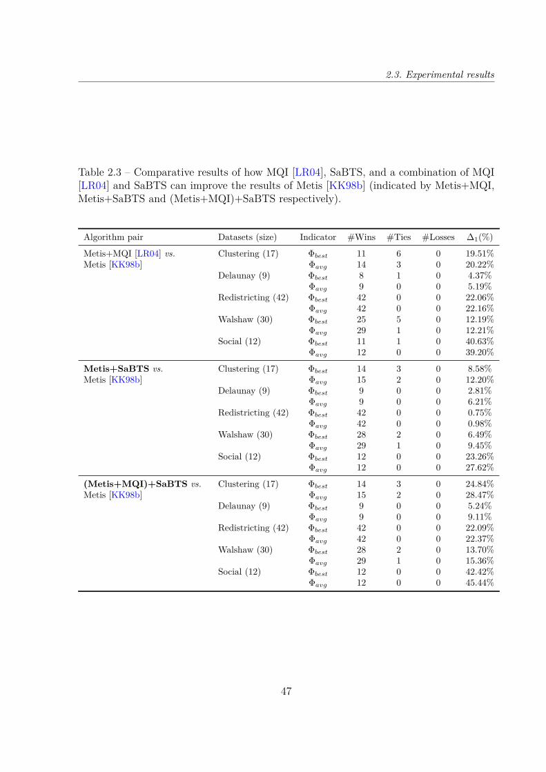
2.3. Experimental results
Table 2.3 – Comparative results of how MQI [LR04], SaBTS, and a combination of MQI[LR04] and SaBTS can improve the results of Metis [KK98b] (indicated by Metis+MQI,Metis+SaBTS and (Metis+MQI)+SaBTS respectively).
Algorithm pair Datasets (size) Indicator #Wins #Ties #Losses ∆1(%)
Metis+MQI [LR04] vs.Metis [KK98b]
Clustering (17) Φbest 11 6 0 19.51%Φavg 14 3 0 20.22%
Delaunay (9) Φbest 8 1 0 4.37%Φavg 9 0 0 5.19%
Redistricting (42) Φbest 42 0 0 22.06%Φavg 42 0 0 22.16%
Walshaw (30) Φbest 25 5 0 12.19%Φavg 29 1 0 12.21%
Social (12) Φbest 11 1 0 40.63%Φavg 12 0 0 39.20%
Metis+SaBTS vs.Metis [KK98b]
Clustering (17) Φbest 14 3 0 8.58%Φavg 15 2 0 12.20%
Delaunay (9) Φbest 9 0 0 2.81%Φavg 9 0 0 6.21%
Redistricting (42) Φbest 42 0 0 0.75%Φavg 42 0 0 0.98%
Walshaw (30) Φbest 28 2 0 6.49%Φavg 29 1 0 9.45%
Social (12) Φbest 12 0 0 23.26%Φavg 12 0 0 27.62%
(Metis+MQI)+SaBTS vs.Metis [KK98b]
Clustering (17) Φbest 14 3 0 24.84%Φavg 15 2 0 28.47%
Delaunay (9) Φbest 9 0 0 5.24%Φavg 9 0 0 9.11%
Redistricting (42) Φbest 42 0 0 22.09%Φavg 42 0 0 22.37%
Walshaw (30) Φbest 28 2 0 13.70%Φavg 29 1 0 15.36%
Social (12) Φbest 12 0 0 42.42%Φavg 12 0 0 45.44%
47
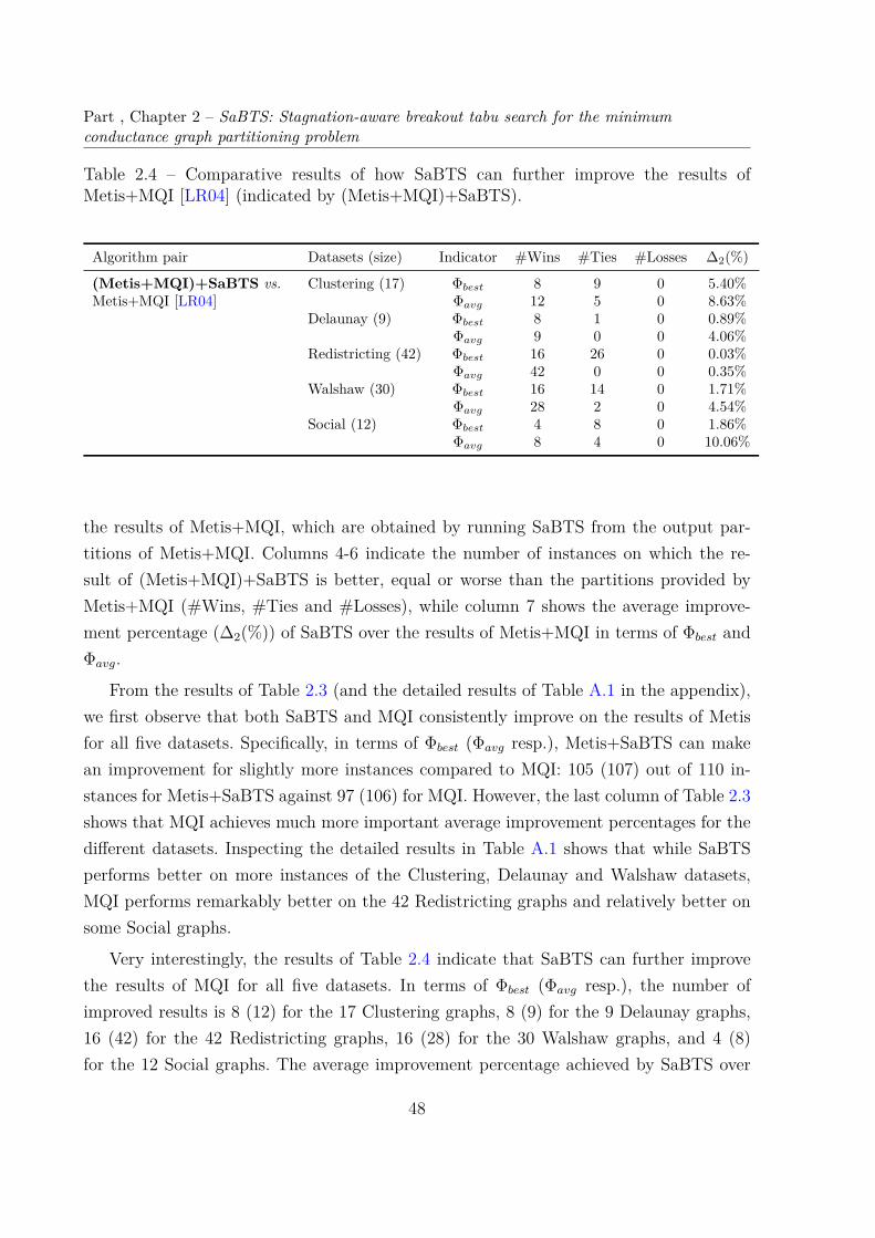
Part , Chapter 2 – SaBTS: Stagnation-aware breakout tabu search for the minimumconductance graph partitioning problem
Table 2.4 – Comparative results of how SaBTS can further improve the results ofMetis+MQI [LR04] (indicated by (Metis+MQI)+SaBTS).
Algorithm pair Datasets (size) Indicator #Wins #Ties #Losses ∆2(%)
(Metis+MQI)+SaBTS vs.Metis+MQI [LR04]
Clustering (17) Φbest 8 9 0 5.40%Φavg 12 5 0 8.63%
Delaunay (9) Φbest 8 1 0 0.89%Φavg 9 0 0 4.06%
Redistricting (42) Φbest 16 26 0 0.03%Φavg 42 0 0 0.35%
Walshaw (30) Φbest 16 14 0 1.71%Φavg 28 2 0 4.54%
Social (12) Φbest 4 8 0 1.86%Φavg 8 4 0 10.06%
the results of Metis+MQI, which are obtained by running SaBTS from the output par-titions of Metis+MQI. Columns 4-6 indicate the number of instances on which the re-sult of (Metis+MQI)+SaBTS is better, equal or worse than the partitions provided byMetis+MQI (#Wins, #Ties and #Losses), while column 7 shows the average improve-ment percentage (∆2(%)) of SaBTS over the results of Metis+MQI in terms of Φbest andΦavg.
From the results of Table 2.3 (and the detailed results of Table A.1 in the appendix),we first observe that both SaBTS and MQI consistently improve on the results of Metisfor all five datasets. Specifically, in terms of Φbest (Φavg resp.), Metis+SaBTS can makean improvement for slightly more instances compared to MQI: 105 (107) out of 110 in-stances for Metis+SaBTS against 97 (106) for MQI. However, the last column of Table 2.3shows that MQI achieves much more important average improvement percentages for thedifferent datasets. Inspecting the detailed results in Table A.1 shows that while SaBTSperforms better on more instances of the Clustering, Delaunay and Walshaw datasets,MQI performs remarkably better on the 42 Redistricting graphs and relatively better onsome Social graphs.
Very interestingly, the results of Table 2.4 indicate that SaBTS can further improvethe results of MQI for all five datasets. In terms of Φbest (Φavg resp.), the number ofimproved results is 8 (12) for the 17 Clustering graphs, 8 (9) for the 9 Delaunay graphs,16 (42) for the 42 Redistricting graphs, 16 (28) for the 30 Walshaw graphs, and 4 (8)for the 12 Social graphs. The average improvement percentage achieved by SaBTS over
48
2.4. Analysis of SaBTS
MQI varies according to the datasets. The improvements are more important for theClustering, Delaunay, Walshaw and Social datasets than for the Redistricting dataset.Finally, the detailed results of Table A.1 in the appendix show that Metis+SaBTS and(Metis+MQI)+SaBTS together cover all the best results in terms of Φbest and Φavg forthe 110 instances tested.
This experiment confirms that 1) it is more advantageous to start SaBTS with asolution from Metis or MQI to obtain still better solutions, and 2) we can jointly applyMetis, MQI and SaBTS to find high quality partitions in terms of low conductance fordivers graphs with different structures.
Finally, even if we do not report more computational results, we mention that we alsotested much larger graphs from the 10th DIMACS Challenge Benchmark with 8× 10⁵ to1.4 × 107 vertices. We observed that SaBTS can improve the partitions given by Metisand MQI.
2.4 Analysis of SaBTS
In this section, we first analyze the effect of the parameters on the performance ofSaBTS, and then investigate the impact of the constrained neighborhood in the tabusearch, and lastly provide some insights into the adaptive perturbation strategy. Thesestudies are based on 10 challenging instances selected from the 110 benchmark instances:PGPgiantcompo, preferentialAttachment, delaunay_n16, delaunay_n17, sd2010, ms2010,wing, brack2, gplus_2000, pokec_20000. As before, we independently solve 20 times eachinstance with a cutoff time of 60 minutes, each run being started with an initial solutiongenerated with the greedy method of Section 2.2.2.
2.4.1 Effect of the parameters
The proposed SaBTS algorithm has five parameters: the tabu tenure managementfactor α, depth of tabu search D, stagnation threshold T , initial jump magnitude L0 andminimum probability P0. To investigate the effect of each parameter on the performanceof the algorithm, we vary its value within a reasonable range, while maintaining otherparameters to their default values as shown in Table 2.1. We use the following valueranges: α = 40, 60, 80, 100, 120, D = 2000, 4000, 6000, 8000, 10000, T = 1000,3000, 5000, 7000, 9000, L0 = 0.3, 0.4, 0.5, 0.6, 0.7×|V | and P0 = 0.65, 0.70, 0.75, 0.80,
49
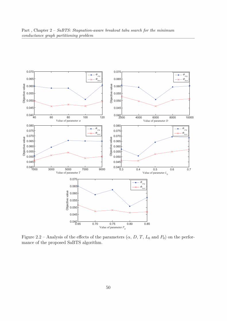
Part , Chapter 2 – SaBTS: Stagnation-aware breakout tabu search for the minimumconductance graph partitioning problem
D
avg
best
avg
best
T L0
avg
best
avg
best
P0
avg
best
Figure 2.2 – Analysis of the effects of the parameters (α, D, T , L0 and P0) on the perfor-mance of the proposed SaBTS algorithm.
50
2.4. Analysis of SaBTS
0.85. Figure 2.2 shows the behavior of SaBTS with respect to each of the parameters,where the X-axis indicates the values of each parameter and the Y-axis shows the best/average objective values over the 10 tested instances.
Figure 2.2 indicates that the performance of SaBTS is significantly influenced by thesetting of each parameter. For α, the best performance is attained when α = 100, and a toosmall α value leads to poor performance of SaBTS. This can be explained that a smallα value makes the prohibited time too short and cannot effectively prevent the searchfrom cycling. For D, the value of 6000 is the best choice, and a too large or too small Dvalue deteriorates SaBTS’s performance. Also, SaBTS reaches its best performance witha T value of 1000. However, the performance of SaBTS is not sensitive to an increase ofT . Then for L0, the performance of SaBTS generally decreases as the coefficient of L0
increases and the value of 0.4 shows the best performance, while a too large coefficientvalue will have an effect similar to a random restart. For P0, the best solution is not reallysensitive to P0. Thus we set P0 = 0.8, which leads to the best average solution.
This study justifies the default parameter setting of Table 2.1. We notice that amongthese parameters, D, T and L0 are a little more sensitive than α and P0. Therefore, if theuser needs to tune the parameters, effort should be put on D, T and L0.
2.4.2 Impact of the constrained neighborhood on tabu seach
As explained in Section 2.2.3, the constrained neighborhood based on critical verticesis a key component of the tabu search procedure. In this experiment, we highlight itsinterest by comparing the SaBTS procedure with a SaBTS variant (called SaBTSno_cons)where we replace the constrained neighborhood (see Equation (2.3)) by the unconstrainedneighborhood defined by equation (2.1) and keep the other components unchanged. Werun both algorithms 20 times to solve each of the 10 instances used in the last sectionand report the results in Table 2.5.
In Table 2.5, we indicate for each instance the gap of the best and average results ofSaBTSno_cons with respect to the best and average results of SaBTS. The p-values fromthe Wilcoxon signed-rank test are shown in the last row of the table. For example, for theinstance PGPgiantcompo, SaBTSno_cons has worse results in terms of Φbest and Φavg with abest and average gap of 0.0093 and 0.0113 respectively compared to the best and averagevalues of SaBTS. From the table, we observe that SaBTS dominates SaBTSno_cons foreach tested instance both in terms of best and average solutions. The p-values from theWilcoxon signed-rank test also confirm the dominance of SaBTS over SaBTSno_cons. This
51

Part , Chapter 2 – SaBTS: Stagnation-aware breakout tabu search for the minimumconductance graph partitioning problem
Table 2.5 – Comparison of SaBTS with a variant SaBTSno_cons using the unconstrainedneighborhood.
Instance SaBTSno_cons
∆Φbest ∆Φavg
PGPgiantcompo +0.0093 +0.0113preferentialAttachment +0.0006 +0.0018delaunay_n16 +0.0008 +0.0001delaunay_n17 +0.0392 +0.0337sd2010 +0.0039 +0.0052ms2010 +0.0070 +0.0139wing +0.0065 +0.0088brack2 +0.0002 +0.0035gplus_2000 0 +0.0014pokec_20000 +0.0004 +0.0010
p-value 2.00e-03 2.00e-03
experiment demonstrates the usefulness and effectiveness of the constrained neighborhoodfor the SaBTS algorithm.
2.4.3 Impact of the perturbation strategy
As mentioned in Section 2.2.4, the perturbation procedure aims to diversify the searchand help the search process to escape local optima traps. In order to highlight the contribu-tion of the adopted perturbation strategy to the overall performance, we create three vari-ants of SaBTS by varying the perturbation mechanism. The first variant (called SaBTSD3)only employs the random perturbation. The second variant (called SaBTSD1+D2) disablesthe random perturbation, but keeps the frequency based perturbation and the cut edgebased swap perturbation. The last variant (called SaBTSD2+D3) disables the frequencybased perturbation, but keeps the cut edge based swap perturbation and the randomperturbation. For all the variants, we keep the other components of SaBTS unchanged.
Table 2.6 shows the best and average result gap of each SaBTS variant with referenceto the result of SaBTS. The p-values from the Wilcoxon signed-rank test are given in thelast row. First, SaBTS significantly dominates SaBTSD3 by reaching the best and averageresults for 9 out of 10 instances (p = 0.0020 for Φbest and p = 0.0039 for Φavg). Second,compared to SaBTSD1+D2, SaBTS performs marginally better in terms of Φbest (winning7 instances with p = 0.0645) and significantly better than in terms of Φavg (winning 10
52

2.5. Conclusion
Table 2.6 – Comparison of SaBTS with three variants SaBTSD3, SaBTSD1+D2 andSaBTSD2+D3 applying different perturbation schemes.
Instance SaBTSD3 SaBTSD1+D2 SaBTSD2+D3∆Φbest ∆Φavg ∆Φbest ∆Φavg ∆Φbest ∆Φavg
PGPgiantcompo +0.0035 +0.0026 +0.0032 +0.0180 -0.0009 -0.0010preferentialAttachment +0.0095 +0.0117 +0.0143 +0.2373 +0.2882 +0.3152delaunay_n16 +0.0083 +0.0077 +0.0012 +0.0035 -0.0003 0delaunay_n17 +0.0011 +0.0088 -0.0062 +0.0037 -0.0070 +0.0089sd2010 +0.0064 +0.0130 -0.0002 +0.0058 -0.0005 +0.0041ms2010 +0.0150 +0.0176 +0.0009 +0.0097 +0.0006 +0.0202wing +0.0070 +0.0061 -0.0009 +0.0082 -0.0018 +0.0060brack2 +0.0012 +0.0028 +0.0148 +0.0295 +0.0126 +0.0184gplus_2000 0 -0.0001 +0.0083 +0.0178 0 +0.0003pokec_20000 +0.0007 +0.0004 +0.0141 +0.0893 +0.0004 +0.0049
p-value 2.00e-03 3.90e-03 6.45e-02 2.00e-03 1.00e-00 9.80e-03
instances with p = 0.0020). Third, compared to SaBTSD2+D3, even if SaBTS does notshow any advantage in terms of Φbest, SaBTS has a clear dominance in terms of Φavg
(p = 0.0098). This experiment thus confirms the interest of the adopted perturbationstrategy compared to alternative strategies.
2.5 Conclusion
This chapter introduced a stagnation-aware breakout tabu search algorithm (SaBTS)for the minimum conductance graph partitioning problem (MC-GPP). As the first algo-rithm adapting the breakout local search framework to MC-GPP, SaBTS distinguishes it-self from existing MC-GPP algorithms mainly by two noteworthy features: the constrainedneighborhood tabu search procedure and the self-adaptive and multi-strategy perturba-tion procedure. We performed a large scale computational study to assess the performanceof the proposed SaBTS algorithm and investigated its key components (parameters, con-strained neighborhood, perturbation strategy) to gain insights on the functioning of thealgorithm.
The computational study on five datasets of 110 benchmark graphs with up to around500,000 vertices allows us to draw the following conclusions.
— SaBTS with greedy initial solutions (Greedy+SaBTS) dominates the recent StS-
53

Part , Chapter 2 – SaBTS: Stagnation-aware breakout tabu search for the minimumconductance graph partitioning problem
AMA algorithm dedicated to MC-GPP [Cha17] both in terms of the best and averageresults.
— SaBTS with greedy initial solutions (Greedy+SaBTS) and the popular graph parti-tioning tool Metis (version 5.1.0) [KK98b] perform well on different datasets. Glob-ally there is no clear dominance of one method over the other. When SaBTS is usedto refine the results of Metis, it consistently improves the partitions provided byMetis for 108 out of the 110 benchmark graphs.
— When SaBTS is used as a post-processing procedure of Metis and is compared to thestate-of-the-art max-flow based method MQI [LR04], SaBTS improves the result ofMetis on slightly more graphs than MQI, but MQI achieves much more importantquality improvement.
— When SaBTS is used as a post-processing procedure of MQI, it consistently improvesthe partitions provided by MQI, raising the partition quality for the tested datasets.
— SaBTS and existing methods like Metis and MQI can be advantageously used in acombined way, helping to find high quality partitions for graphs with very differentstructures and characteristics.
54
Chapter 3
MAMC: A HYBRID EVOLUTIONARY
ALGORITHM FOR FINDING LOW
CONDUCTANCE OF LARGE GRAPHS
3.1 Introduction
In this chapter, we aim to enrich the toolkit of practical solution methods for MC-GPP. For this purpose, we introduce a novel hybrid evolutionary algorithm called MAMCwhich is able to find high quality solutions of low conductance for large graphs. Specifi-cally, the proposed MAMC algorithm integrates a set of complementary components tojointly ensure its search effectiveness and computational efficiency. We summarize themain contributions of this work as follows.
— First, the hybrid evolutionary algorithm presented in this work takes advantage ofpopulation-based global search and local optimization. Specifically, while it adoptsa standard crossover operator to generate offspring solutions, the proposed MAMCalgorithm integrates an innovative progressive local search procedure to cope withthe difficulty raised by large graphs (with at least 5 × 10⁴ vertices). To ensure ahealthy population of both high diversity and quality, the algorithm uses a mixedtechnique for population initialization and a proven distance-and-quality based poolupdating strategy for population management.
— Second, we perform extensive computational assessments on 60 large-scale real worldbenchmark instances (including 50 graphs from the 10th DIMACS ImplementationChallenge Benchmark and 10 graphs from the Network Data Repository online, withup to 23 million vertices). We demonstrate the high competitiveness of the proposedMAMC algorithm compared to four state-of-the-art algorithms. As an additionalassessment, we show an application of using the proposed IMSA algorithm to detect
55

Part , Chapter 3 – MAMC: A hybrid evolutionary algorithm for finding low conductance oflarge graphs
community structures in complex networks.
— Third, this work advances the state-of-the-art in terms of effective solving of thegeneral minimum conductance graph partitioning problem. The ideas of some un-derlying algorithmic components are of general interest and could be advantageouslyadapted to design effective algorithms for other large graph optimization problems.
The chapter is organized as follows. Section 3.2 describes the proposed MAMC al-gorithm and its ingredients. Section 3.3 presents computational studies and comparisonsbetween the proposed MAMC algorithm and state-of-the-art algorithms. Section 3.4 an-alyzes the key algorithmic components. We draw concluding remarks in the last section.
3.2 A hybrid evolutionary algorithm for finding lowconductance of large graphs
3.2.1 General Outline
Hybrid evolutionary algorithms are known to be a powerful and proven tool for nu-merous NP-hard problems (e.g., graph partitioning [BH11a; GBF11; WH13], quadraticassignment [BH15], graph coloring [MG18; PHK10], and unconstrained binary quadraticprogramming [LGH10]) as well as many practical problems (e.g., service placement in fogarchitectures [GLJ19], roadside unit deployment [Mou+18] and task scheduling and dataassignment on clouds [Tey+17]). In this work, we present a hybrid evolutionary algorithmfor tackling MC-GPP, which relies particularly on the memetic computing framework[NCM11]. The proposed algorithm (denoted by MAMC, see Algorithm 4) is composed offour main components: quality-and-diversity based population initialization, recombina-tion operator, progressive constrained neighborhood tabu search and distance-and-qualitybased pool updating procedure.
From an initial population Pop of p solutions (Algorithm 4, line 1), the best solution s∗
among the population is first recorded (line 2). The algorithm then enters into the ‘repeat’loop to improve the population (lines 3-18). At each loop, MAMC selects two parentsolutions at random and applies the double-point crossover to generate two offspring s1
and s2 (lines 4-5). Subsequently, the offspring solutions are improved by the progressiveconstrained neighborhood tabu search procedure (lines 7 and 13). The improved offspringsolutions are used to update the population according to the quality-and-distance based
56
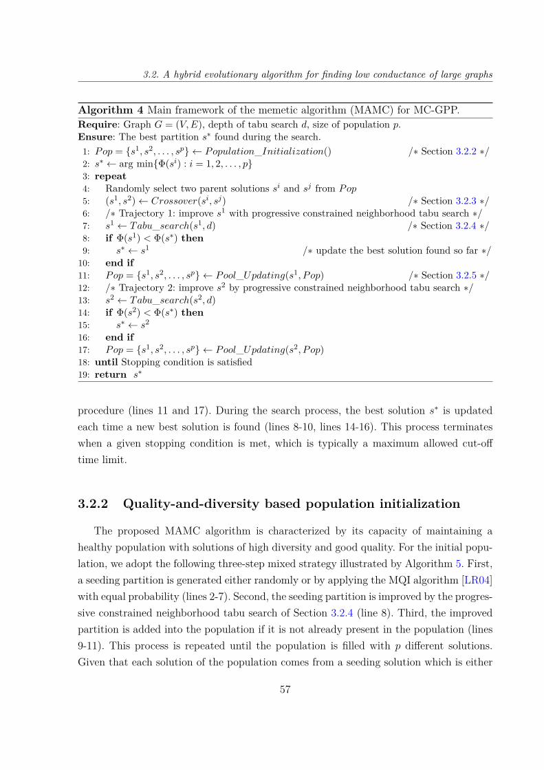
3.2. A hybrid evolutionary algorithm for finding low conductance of large graphs
Algorithm 4 Main framework of the memetic algorithm (MAMC) for MC-GPP.Require: Graph G = (V,E), depth of tabu search d, size of population p.Ensure: The best partition s∗ found during the search.1: Pop = s1, s2, . . . , sp ← Population_Initialization() /∗ Section 3.2.2 ∗/2: s∗ ← arg minΦ(si) : i = 1, 2, . . . , p3: repeat4: Randomly select two parent solutions si and sj from Pop5: (s1, s2)← Crossover(si, sj) /∗ Section 3.2.3 ∗/6: /∗ Trajectory 1: improve s1 with progressive constrained neighborhood tabu search ∗/7: s1 ← Tabu_search(s1, d) /∗ Section 3.2.4 ∗/8: if Φ(s1) < Φ(s∗) then9: s∗ ← s1 /∗ update the best solution found so far ∗/10: end if11: Pop = s1, s2, . . . , sp ← Pool_Updating(s1, Pop) /∗ Section 3.2.5 ∗/12: /∗ Trajectory 2: improve s2 by progressive constrained neighborhood tabu search ∗/13: s2 ← Tabu_search(s2, d)14: if Φ(s2) < Φ(s∗) then15: s∗ ← s2
16: end if17: Pop = s1, s2, . . . , sp ← Pool_Updating(s2, Pop)18: until Stopping condition is satisfied19: return s∗
procedure (lines 11 and 17). During the search process, the best solution s∗ is updatedeach time a new best solution is found (lines 8-10, lines 14-16). This process terminateswhen a given stopping condition is met, which is typically a maximum allowed cut-offtime limit.
3.2.2 Quality-and-diversity based population initialization
The proposed MAMC algorithm is characterized by its capacity of maintaining ahealthy population with solutions of high diversity and good quality. For the initial popu-lation, we adopt the following three-step mixed strategy illustrated by Algorithm 5. First,a seeding partition is generated either randomly or by applying the MQI algorithm [LR04]with equal probability (lines 2-7). Second, the seeding partition is improved by the progres-sive constrained neighborhood tabu search of Section 3.2.4 (line 8). Third, the improvedpartition is added into the population if it is not already present in the population (lines9-11). This process is repeated until the population is filled with p different solutions.Given that each solution of the population comes from a seeding solution which is either
57
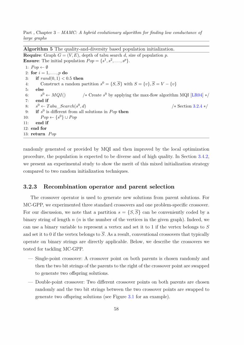
Part , Chapter 3 – MAMC: A hybrid evolutionary algorithm for finding low conductance oflarge graphs
Algorithm 5 The quality-and-diversity based population initialization.Require: Graph G = (V,E), depth of tabu search d, size of population p.Ensure: The initial population Pop = s1, s2, . . . , sp.1: Pop← ∅2: for i = 1, . . . , p do3: if rand(0, 1) < 0.5 then4: Construct a random partition s0 = S, S with S = v, S = V − v5: else6: s0 ←MQI() /∗ Create s0 by applying the max-flow algorithm MQI [LR04] ∗/7: end if8: s0 ← Tabu_Search(s0, d) /∗ Section 3.2.4 ∗/9: if s0 is different from all solutions in Pop then10: Pop← s0 ∪ Pop11: end if12: end for13: return Pop
randomly generated or provided by MQI and then improved by the local optimizationprocedure, the population is expected to be diverse and of high quality. In Section 3.4.2,we present an experimental study to show the merit of this mixed initialization strategycompared to two random initialization techniques.
3.2.3 Recombination operator and parent selection
The crossover operator is used to generate new solutions from parent solutions. ForMC-GPP, we experimented three standard crossovers and one problem-specific crossover.For our discussion, we note that a partition s = S, S can be conveniently coded by abinary string of length n (n is the number of the vertices in the given graph). Indeed, wecan use a binary variable to represent a vertex and set it to 1 if the vertex belongs to Sand set it to 0 if the vertex belongs to S. As a result, conventional crossovers that typicallyoperate on binary strings are directly applicable. Below, we describe the crossovers wetested for tackling MC-GPP.
— Single-point crossover: A crossover point on both parents is chosen randomly andthen the two bit strings of the parents to the right of the crossover point are swappedto generate two offspring solutions.
— Double-point crossover: Two different crossover points on both parents are chosenrandomly and the two bit strings between the two crossover points are swapped togenerate two offspring solutions (see Figure 3.1 for an example).
58
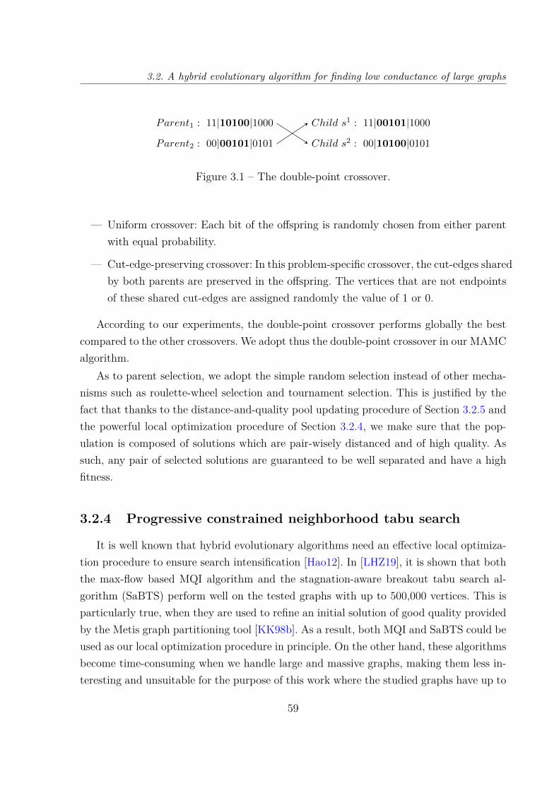
3.2. A hybrid evolutionary algorithm for finding low conductance of large graphs
Parent1 : 11|10100|1000 Child s1 : 11|00101|1000
Parent2 : 00|00101|0101 Child s2 : 00|10100|0101
Figure 3.1 – The double-point crossover.
— Uniform crossover: Each bit of the offspring is randomly chosen from either parentwith equal probability.
— Cut-edge-preserving crossover: In this problem-specific crossover, the cut-edges sharedby both parents are preserved in the offspring. The vertices that are not endpointsof these shared cut-edges are assigned randomly the value of 1 or 0.
According to our experiments, the double-point crossover performs globally the bestcompared to the other crossovers. We adopt thus the double-point crossover in our MAMCalgorithm.
As to parent selection, we adopt the simple random selection instead of other mecha-nisms such as roulette-wheel selection and tournament selection. This is justified by thefact that thanks to the distance-and-quality pool updating procedure of Section 3.2.5 andthe powerful local optimization procedure of Section 3.2.4, we make sure that the pop-ulation is composed of solutions which are pair-wisely distanced and of high quality. Assuch, any pair of selected solutions are guaranteed to be well separated and have a highfitness.
3.2.4 Progressive constrained neighborhood tabu search
It is well known that hybrid evolutionary algorithms need an effective local optimiza-tion procedure to ensure search intensification [Hao12]. In [LHZ19], it is shown that boththe max-flow based MQI algorithm and the stagnation-aware breakout tabu search al-gorithm (SaBTS) perform well on the tested graphs with up to 500,000 vertices. This isparticularly true, when they are used to refine an initial solution of good quality providedby the Metis graph partitioning tool [KK98b]. As a result, both MQI and SaBTS could beused as our local optimization procedure in principle. On the other hand, these algorithmsbecome time-consuming when we handle large and massive graphs, making them less in-teresting and unsuitable for the purpose of this work where the studied graphs have up to
59

Part , Chapter 3 – MAMC: A hybrid evolutionary algorithm for finding low conductance oflarge graphs
Algorithm 6 Progressive constrained neighborhood tabu search (PCNTS).Require: Graph G = (V,E), current solution s, depth of tabu search d.Ensure: The best solution found sb.1: sb ← s /∗ record the best solution found during the current TS run ∗/2: H ← ∅3: β ← 0 /∗ counter of consecutive non-improving iterations w.r.t. sb ∗/4: ev ← 1 /∗ ev is the number of evaluating vertices in NC(s) ∗/5: Create the set CV (s, ev) of critical vertices6: while β < d do7: Select a best eligible vertex v in CV (s, ev)8: s← s⊕Relocate(v)9: Update the set of critical vertices CV (s, ev)10: Update tabu list H[v] with tabu tenure tt11: if Φ(s) < Φ(sb) then12: sb ← s13: β ← 0, ev ← 114: else15: β ← β + 1, ev ← ev + 116: end if17: if ev > |CV (s)| then18: ev = 119: end if20: end while21: return sb
60

3.2. A hybrid evolutionary algorithm for finding low conductance of large graphs
23 million vertices. To be able to cope with such large graphs, we created the progressiveconstrained neighborhood tabu search algorithm (PCNTS) that is presented below.
Basically, our PCNTS procedure uses the ‘Relocate’ operator to explore “critical” ver-tices [LHZ19]. Specifically, let s = S, S be the incumbent solution and v a vertex, thenRelocate(v) transforms s to a new (neighbor) solution s′ (denoted by s′ = s⊕Relocate(v))by displacing vertex v from its current set S or S to the complement set. For the purpose ofconductance minimization, it is unnecessary to consider a vertex for relocation if the vertexis not the endpoint of a cut edge [LHZ19]. As a result, we identify the set CV (s) of can-didate vertices for relocation as CV (s) = v ∈ V : v is the endpoint of a cut edge of s.Note that even if the set CV (s) is much smaller than the set of vertices V , examining allcritical vertices at each iteration of the algorithm (this is what SaBTS of [LHZ19] does)can still become very expensive for large and massive graphs. This is especially true whenthe given graph is dense, because in this case, any partition will have a high number of cutedges, thus implying many critical vertices. Moreover, as discussed in [Cha17; LHZ19],unlike the conventional graph k-way partitioning problem where examining all ‘Relocate’neighbor solutions can be performed in O(1), no technique is known to ensure such anefficiency for performing ‘Relocate’ for MC-GPP. This implies that the cost of examin-ing neighbor solutions is proportionally correlated to the number of critical vertices andbecomes prohibitive for large graphs.
To cope with this difficulty, we devise the following progressive and elastic neigh-borhood exploration strategy which dynamically increases or decreases the number ofexamined critical vertices according to a well-defined condition (see Algorithm 6). Specif-ically, we start with one critical vertex (indicated by ev = 1, ev is a counter indicating thenumber of the critical vertices to be examined). If relocating this vertex at the currentiteration does not lead to a solution better than the recorded local best solution (sb),we increase ev by one, implying that during the next iteration, one more critical vertexwill be examined. As a result, as long as no improved local best solution is found, a stilllarger neighborhood exploration is enabled by increasing ev (i.e., the number of candidatecritical vertices) during the next iteration. During the search, ev is reset to one as soonas the recorded local best solution (sb) is updated or ev reaches its upper limit |CV (s)|.The progressive constrained neighborhood tabu search procedure thus explores an elasticneighborhood NAC(s) whose size is dynamically adjusted by the counter ev according to
61

Part , Chapter 3 – MAMC: A hybrid evolutionary algorithm for finding low conductance oflarge graphs
the search state.
NAC(s) = s′ : s⊕Relocate(v), v ∈ CV (s, ev), 1 ≤ ev ≤ |CV (s)| (3.1)
where CV (s, ev) ⊂ CV (s) is the set of critical vertices to be examined.Thus, by examining the neighborhood NAC(s) induced by CV (s, ev) instead of the
whole neighborhood induced by CV (s), the PCNTS procedure increases its computationalefficiency considerably.
For a given neighbor solution s′ in the neighborhoodNAC(s), it is necessary to quantifythe conductance variation (called move gain) δ(v) = Φ(s′)−Φ(s) with Φ(s) already known.This can be performed in O(1) time by simply calculating |cut(s′)|, vol(S ′), vol(S ′) asfollows [Cha17; LHZ19].
|cut(s′)| = |cut(s)|+ degS(v)− degS(v) (3.2)
vol(S ′) = vol(S)− deg(v) (3.3)
vol(S ′) = vol(S) + deg(v) (3.4)
where s′ = S ′, S ′ with S ′ = S \ v, S ′ = S ∪ v is the neighbor solution afterrelocating v from S to S of the solution s = S, S.
To explore the progressive constrained neighborhood NAC(s), the PCNTS procedurefirst identifies the set CV (s, ev) with one critical vertex (Algorithm 6, line 5). This can beachieved in O(1) time. Then at each iteration, PCNTS selects one best vertex v in termsof move gain achieved in O(|CV (s, ev)|) time among the eligible critical vertices (ties arebroken randomly) and relocates v to obtain a neighbor solution. A vertex qualifies aseligible if it is not forbidden by the tabu list (see below). Note that if a vertex leading to asolution better than the recorded best solution sb is always selected, even if it is forbiddenby the tabu list (this is called the aspiration criterion in tabu search).
It is possible that the above search procedure revisits a previously encountered solu-tion, thus leading to search cycling. To prevent this, we use a memory H (called tabulist) to record each displaced vertex and forbid the vertex to be relocated again during aspecific number tt of iterations (called tabu tenure). Thus, each time a vertex v ∈ CV isrelocated to generate a neighbor solution, the PCNTS procedure adds v in H (an integer
62
3.2. A hybrid evolutionary algorithm for finding low conductance of large graphs
vector in our case) and will ignore this vertex for next tt(v) iterations. In practice, when vis relocated, H[v] is set to iter+ tt where iter represents the current number of iterations.Then during the next iterations, if iter < H[v], v is forbidden by the tabu list; otherwise,v is not prohibited by the tabu list.
For the tabu tenure, we adopt the dynamic technique introduced in [GBF11] whichhas proven to be quite robust and effective for graph partitioning problems [LHZ19;WH13]. This technique varies tt with a periodic step function F defined over the cur-rent iteration number iter. For each period, it takes p = 15 successive values (alsocalled intervals). The values are separated by the interval margins which are definedby x1 = 1, and xi+1 = xi + 100. tt equals F (iter), which is given by (yi)i=1,2,...,15 =α × (10, 20, 10, 40, 10, 20, 10, 80, 10, 20, 10, 40, 10, 20, 10) (α is a parameter). Therefore, ttequals 10 × α between iterations 1 and 100, 20 × α between iterations 101 and 200, etc.Our experiments confirmed that this technique makes the algorithm quite robust acrossthe tested instances and avoids the difficulties of manually tuning the tabu tenure.
3.2.5 Distance-and-quality based pool updating procedure
Population diversity is critical to avoid a premature convergence of an evolutionaryalgorithm. To maintain a healthy population of our algorithm, we employ a diversificationpreserving strategy [LGH10] to update the population with each new offspring solution.This strategy considers not only the quality of each offspring solution, but also its distanceto the existing solutions of the population.
Following [PHK10], we use the well-known set-theoretic partition distance [Gus02]to measure the distance dab between two solutions sa and sb. The partition distance isthe minimum number of one-move steps necessary to transform one solution to anothersolution. For the given population Pop, we calculate Di,Pop = mindij|sj ∈ Pop, j 6=i, i, j = 1, . . . , |Pop|.
Then, we determine the ‘worst’ solution in the population, according to the followinggoodness score function which considers both quality and distance:
g(si, Pop) = γA(Φ(si)) + (1− γ)A(Di,Pop) (3.5)
where γ is a parameter set to 0.6 according to [LGH10] and Φ(si) is the objective
63
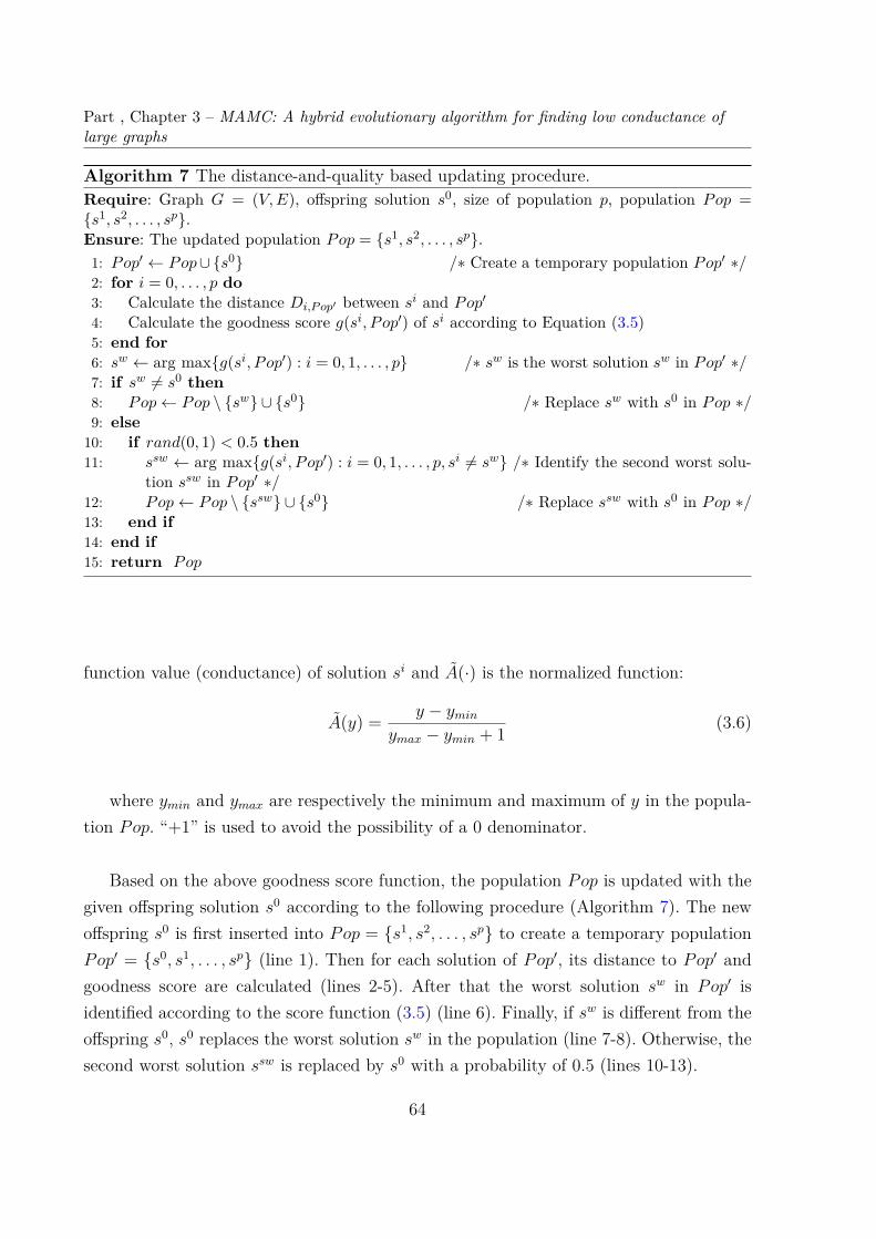
Part , Chapter 3 – MAMC: A hybrid evolutionary algorithm for finding low conductance oflarge graphs
Algorithm 7 The distance-and-quality based updating procedure.Require: Graph G = (V,E), offspring solution s0, size of population p, population Pop =s1, s2, . . . , sp.Ensure: The updated population Pop = s1, s2, . . . , sp.1: Pop′ ← Pop∪s0 /∗ Create a temporary population Pop′ ∗/2: for i = 0, . . . , p do3: Calculate the distance Di,Pop′ between si and Pop′4: Calculate the goodness score g(si, Pop′) of si according to Equation (3.5)5: end for6: sw ← arg maxg(si, Pop′) : i = 0, 1, . . . , p /∗ sw is the worst solution sw in Pop′ ∗/7: if sw 6= s0 then8: Pop← Pop \ sw ∪ s0 /∗ Replace sw with s0 in Pop ∗/9: else10: if rand(0, 1) < 0.5 then11: ssw ← arg maxg(si, Pop′) : i = 0, 1, . . . , p, si 6= sw /∗ Identify the second worst solu-
tion ssw in Pop′ ∗/12: Pop← Pop \ ssw ∪ s0 /∗ Replace ssw with s0 in Pop ∗/13: end if14: end if15: return Pop
function value (conductance) of solution si and A(·) is the normalized function:
A(y) = y − yminymax − ymin + 1 (3.6)
where ymin and ymax are respectively the minimum and maximum of y in the popula-tion Pop. “+1” is used to avoid the possibility of a 0 denominator.
Based on the above goodness score function, the population Pop is updated with thegiven offspring solution s0 according to the following procedure (Algorithm 7). The newoffspring s0 is first inserted into Pop = s1, s2, . . . , sp to create a temporary populationPop′ = s0, s1, . . . , sp (line 1). Then for each solution of Pop′, its distance to Pop′ andgoodness score are calculated (lines 2-5). After that the worst solution sw in Pop′ isidentified according to the score function (3.5) (line 6). Finally, if sw is different from theoffspring s0, s0 replaces the worst solution sw in the population (line 7-8). Otherwise, thesecond worst solution ssw is replaced by s0 with a probability of 0.5 (lines 10-13).
64
3.3. Experimental results
3.3 Experimental results
In this section, we first assess the proposed MAMC algorithm for tackling MC-GPPbased on two sets of 60 benchmark graphs from various applications, and then applyMAMC to detect communities of 3 complex real world networks.
3.3.1 Benchmark instances
The two sets of benchmarks include 60 large and massive graphs which are from twosources and have 54,870 to 23,947,347 vertices, and one set of 3 complex real world networkgraphs from the application of community detection.
— The 10th DIMACS Implementation Challenge Benchmark 1.This datasetcontains 50 graphs which are dedicated to two related problems of graph partition-ing and graph clustering [Bad+14; Bad+13]. These graphs belong to 6 families:Clustering instances, Delaunay graphs, Redistricting, Walshaw’s graph partitioningarchive, Co-author and citation networks, and Sparse matrices.
— The Network Data Repository online 2. This dataset contains 10 massive realworld network graphs [RA15].
— The complex real-world network 3. This dataset contains 3 complex real worldnetwork graphs for community detection.
3.3.2 Experimental setting
The proposed MAMC algorithm was coded in C++ 4 and compiled using GNU g++6.3.0 compiler with the “-O3” flag. The experiments were conducted on a computer run-ning Ubuntu Linux 16.04, using 6 cores of AMD Opteron 4184 CPU @ 2.80GHz and32GByte RAM.
To evaluate our results, we adopt as our references the following four state-of-the-artalgorithms in the literature.
— Metis [KK98b]: This is a general and popular graph partitioning package whichhas been used to generate partitions in several studies on the MC-GPP [AL08;
1. https://www.cc.gatech.edu/dimacs10/downloads.shtml2. http://networkrepository.com/index.php3. http://www-personal.umich.edu/~mejn/netdata/4. The code of our MAMC algorithm is available at: http://www.info.univ-angers.fr/~hao/mamc.
html
65

Part , Chapter 3 – MAMC: A hybrid evolutionary algorithm for finding low conductance oflarge graphs
Table 3.1 – Parameter setting of the proposed MAMC algorithm.
Parameter Section Description Value
p §3.2.2 Population size 20α §3.2.4 Tabu tenure management factor 10d §3.2.4 Depth of tabu search 6000
LR04; Les+09]. As shown in [LHZ19], even if Metis does not directly optimizethe conductance criterion (it minimizes the number of cut edges), it can producepartitions of relatively low conductance within a very short computation time. Inour study, Metis is used to serves as a baseline reference, as well as to create initialpartitions of the MQI and SaBTS methods (see below). For this work, we used thelatest release Metis 5.1.0 5.
— MQI [LR04]: This is a max-flow quotient-cut improvement algorithm which refines agiven initial partition. In previous studies and this work, MQI starts with a partitionprovided by the fast Metis tool. To our knowledge, MQI is one of the best algorithmsfor the MC-GPP. We used the latest implementation of MQI 6.
— SaBTS [LHZ19]: This is the most recent metaheuristic algorithm for the MC-GPP,which combines a dedicated tabu search procedure and a self-adaptive perturba-tion procedure. The intensive experiments reported in [LHZ19] show that SaBTSis able to consistently improve a partition provided by Metis and can also reducethe conductance of partitions given by MQI (see below). We used the source codeof SaBTS 7.
— MQI+SaBTS [LHZ19]: This hybrid approach uses SaBTS to refine a partitionproduced by MQI. Thanks to the combination of these two powerful approaches(MQI and SaBTS), MQI+SaBTS performs the best compared to other existingapproaches.
The proposed MAMC algorithm requires 3 parameters: population size p, tabu tenuremanagement factor α and depth of tabu search d. Following previous studies [GBF11;WH13], we adopted a small population size and set p = 20. For α and d, they were fixedaccording to the analysis reported in Section 3.4.1. For our experiments, we consistently
5. http://glaros.dtc.umn.edu/gkhome/metis/metis/overview6. https://github.com/kfoynt/LocalGraphClustering7. http://www.info.univ-angers.fr/~hao/mcgpp.html
66

3.3. Experimental results
used the parameter setting shown in Table 3.1 to run our MAMC algorithm to solveall instances. This parameter setting can also be considered to be the default setting ofMAMC.
For a fair comparison, we run, on the same computer, our MAMC algorithm and theabove reference algorithms with their respective default parameter setting under the sametime limit of 60 minutes per run and per instance.
3.3.3 Computational results and comparisons on the benchmarkinstances
In this section, we report the results of the proposed MAMC algorithm as well as thefour reference algorithms (Metis [KK98b], MQI [LR04], SaBTS [LHZ19], and MQI+SaBTS[LHZ19]) on 60 benchmark instances. It is worth noting that MQI, SaBTS, and MQI+SaBTSall start from an initial partition provided by Metis. Tables 3.2 and 3.3 provide the detailedresults of the compared algorithms, while Table 3.4 shows a summary.
In Tables 3.2 and 3.3, columns 1-2 indicate the name (Graph) and the number ofvertices (|V |) for each instance. The remaining columns show the results of Metis, MQI,SaBTS, MQI+SaBTS and MAMC according to the following performance indicators: thebest conductance (Φbest) found among 20 runs, the average conductance (Φavg), the successrate (hit) over 20 runs to reach Φbest, the average CPU time in seconds (t(s)) of 20 runsto attain the best results, and the standard deviation (σ) of Φbest. It is worth noting thatcomputation times are provided only for indicative purposes, since it is not meaningfulto compare two computation times if the corresponding algorithms lead to solutions ofdifferent quality.
In Table 3.4, column 1 indicates the pairs of compared algorithms (Algorithm pair).Column 2 gives the total number of instances (#Instance). Column 3 shows the qualityindicators in terms of the best and average conductance (Φbest and Φavg). Columns 4-6count the number of instances on which MAMC achieves a better, equal or worse resultcompared to each reference algorithm (#Wins, #Ties, and #Losses). Column 7 reportsthe p-value from the non-parametric Wilcoxon signed-rank test with a confidence level of99%.
The results of Tables 3.2–3.4 show that MAMC performs remarkably well on all 60benchmark instances. Compared to Metis and MQI and in terms of the main performanceindicators Φbest (Φavg), MAMC finds 54 (60) better and 6 (0) equal results with respect
67
Part , Chapter 3 – MAMC: A hybrid evolutionary algorithm for finding low conductance oflarge graphs
to Metis, and 27 (60) better and 33 (0) equal results with respect to MQI. MAMC alsocompetes very favorably with SaBTS and MQI+SaBTS in terms of Φbest (Φavg) with 53(58) wins, 7 (1) ties and 0 (1) losses compared to SaBTS, and 27 (58) wins, 32 (2) tiesand 1 (0) losses compared to MQI+SaBTS. The small p-values (p-value 0.01) from theWilcoxon signed-rank test further confirm the dominance of MAMC over the referencealgorithm in terms of Φbest and Φavg.
Moreover, in terms of the other performance indicators, we observe that to reach thesame Φbest value, MAMC has always a higher success rate and a shorter computationtime. In many cases, MAMC is even able to find a better solution with a higher hit anda shorter time.
To complete these results, we additionally provide a performance assessment of thealgorithms in a visual way by using a generic benchmarking tool called performanceprofiles [DM02] (the reader is referred to [DM02] for details). Performance profiles enablea rigorous comparison of different algorithms over a large set of benchmark instanceswith regard to a specific performance metric (in our case, Φbest and Φavg respectively).Basically, to compare a set of algorithms S over a set of problems P , we define theperformance ratio by rs,p = Φs,p
minΦs,p: s∈S . If an algorithm s does not solve a problem p,then we simply set rs,p = +∞. Thus, the performance function of an algorithm s is givenby Ps(τ) = |p∈P | rs,p≤τ|
|P| . The value Ps(τ) computes the fraction of problems algorithms can solve with at most τ many times the cost of the best algorithm. Ps(1) correspondsto the number of problems that algorithm s solved faster than, or as fast as the otheralgorithms in S. The value Ps(rf ), for a large enough rf , corresponds to the maximumnumber of problems that algorithm s has solved. The quantities Ps(1) and Ps(rf ) arecalled efficiency and robustness of s respectively.
Figure 3.2 shows the performance profiles of our proposed MAMC algorithm as well asthe reference algorithms which have been drawn with the software perprof-py [SSS16].From the figure, we observe that MAMC has a very good performance, surpassing thefour reference algorithms in terms of conductance value. Indeed, MAMC has the highestvalue of Ps(1) among the compared algorithms, meaning that MAMC can quickly findthe lowest conductance for the tested instances. Besides, MAMC also attains a goodrobustness by quickly solving all the instances (corresponding to the fact that MAMCarrives at Ps(rf ) first).
This experiment thus demonstrates the competitiveness of the proposed MAMC algo-rithm for solving MC-GPP compared to the 4 state-of-the-art reference methods.
68

3.3. Experimental resultsTa
ble3.2–Detailedcompu
tatio
nalresults
ofMAMC
with
tworeferencestate-of-the-art
algorit
hmsM
etis[K
K98b],M
QI
[LR04]o
n50
largegrap
hsfro
m“T
he10th
DIM
ACSIm
plem
entatio
nCha
lleng
eBe
nchm
ark”
and10
largegrap
hsfro
m“T
heNetwo
rkDataRep
osito
ryon
line”.
Instan
ceMetis
[KK98b]
MQI[LR04]
MA
MC
Graph
|V|
Φb
es
tΦ
av
ghi
tt(s)
σΦ
be
st
Φa
vg
hit
t(s)
σΦ
be
st
Φa
vg
hit
t(s)
σ
preferential
Attachm
ent
100000
0.31136208
0.33179699
1/20
08.45e-03
0.31132997
0.33039853
1/20
47.91e-03
0.2
87
17
31
80.
2880
4940
1/20
2886
6.17e-04
smallworld
100000
0.11353648
0.11625592
1/20
01.72e-03
0.11322141
0.11604861
1/20
91.72e-03
0.0
99
48
25
90.10321531
1/20
2739
1.27e-03
cnr-2000
325557
0.00014499
0.00045316
1/20
02.30e-04
0.0
00
00
15
60.00000649
12/20
246.76e-06
0.0
00
00
15
60.
0000
0156
20/20
10
eu-2005
862664
0.00180465
0.00297210
1/20
48.45e-04
0.0
00
04
93
00.00064963
5/20
224
8.75e-04
0.0
00
04
93
00.
0000
4930
20/20
110
road
_central
14081816
0.0
00
01
00
00.00001399
1/20
381.52e-06
0.0
00
01
00
00.00001399
1/20
3620
1.52e-06
0.0
00
01
00
00.
0000
1128
9/20
272
1.21e-06
road
_usa
23947347
0.0
00
00
58
40.00000743
1/20
468.70e-07
0.0
00
00
58
40.00000743
1/20
3625
8.70e-07
0.0
00
00
58
40.
0000
0606
11/20
493
2.80e-07
delaun
ay_n1
665536
0.00245485
0.0025
5656
1/20
05.08e-05
0.00233083
0.00239444
1/20
374.40e-05
0.0
02
26
37
60.
0022
9371
1/20
1292
2.44e-05
delaun
ay_n1
7131072
0.00176260
0.00180880
1/20
03.15e-05
0.00161703
0.00166800
1/20
109
1.91e-05
0.0
01
56
85
70.
0016
1819
1/20
2000
2.22e-05
delaun
ay_n1
8262144
0.00122712
0.00128721
1/20
02.50e-05
0.00113731
0.00117238
1/20
251
1.89e-05
0.0
01
13
33
20.
0011
4381
1/20
762
8.03e-06
delaun
ay_n1
9524288
0.00087932
0.00090623
1/20
11.86e-05
0.00078966
0.00081794
1/20
1807
1.16e-05
0.0
00
78
69
30.
0008
0017
1/20
729
9.73e-06
delaun
ay_n2
01048576
0.00062086
0.00064508
1/20
11.26e-05
0.00055891
0.00057390
1/20
3601
9.59e-06
0.00055891
0.00
0561
289/20
273.50e-06
delaun
ay_n2
12097152
0.00043742
0.00045557
1/20
38.39e-06
0.0
00
39
29
30.00041813
1/20
3603
3.01e-05
0.0
00
39
29
30.
0003
9397
8/20
451.35e-06
delaun
ay_n2
24194304
0.0
00
31
35
20.00032532
1/20
86.42
e-06
0.0
00
31
35
20.00032532
1/20
3605
6.42e-06
0.0
00
31
35
20.
0003
1504
13/20
286
2.61e-06
delaun
ay_n2
38388608
0.0
00
22
44
30.00023220
1/20
164.08e-06
0.0
00
22
44
30.00023220
1/20
3611
4.08e-06
0.0
00
22
44
30.
0002
2552
8/20
526
1.30e-06
delaun
ay_n2
416777216
0.0
00
16
18
00.00016509
1/20
312.32e-06
0.0
00
16
18
00.00016509
1/20
3621
2.32e-06
0.0
00
16
18
00.
0001
6208
11/201256
3.20e-07
co2010
201062
0.00067974
0.00073333
1/20
03.29e-05
0.00053701
0.00061163
1/20
116
4.98e-05
0.0
00
53
44
20.
0005
3453
19/20
564
4.80e-07
la2010
204447
0.00037015
0.00042879
1/20
05.70e-05
0.0
00
17
78
90.00028106
3/20
150
7.38e-05
0.0
00
17
78
90.
0001
7789
20/20
40
ia2010
216007
0.00067628
0.00072474
1/20
02.45e-05
0.00060103
0.00062588
1/20
192
1.88e-05
0.0
00
59
14
70.
0006
0046
1/20
1239
4.62e-06
ks2010
238600
0.00058509
0.00063764
1/20
02.36e-05
0.00051471
0.00054122
1/20
226
1.58e-05
0.0
00
51
47
00.
0005
1875
10/20
980
4.54e-06
tn2010
240116
0.00043558
0.00048995
1/20
03.43e-05
0.0
00
33
67
10.00039117
7/20
257
4.45e-05
0.0
00
33
67
10.
0003
3671
20/20
40
az2010
241666
0.00057028
0.00063012
1/20
03.36e-05
0.00044358
0.00051400
1/20
164
4.14e-05
0.0
00
43
83
90.
0004
5183
1/20
941.90e-05
al2010
252266
0.00059056
0.00065367
1/20
03.57e-05
0.00051345
0.00054504
1/20
221
2.70e-05
0.0
00
50
73
20.
0005
1154
2/20
1295
4.01e-06
wi2010
253096
0.00053361
0.00063087
1/20
07.26e-05
0.00049104
0.00053608
1/20
225
4.73e-05
0.0
00
48
24
70.
0004
8581
3/20
1374
4.78e-06
mn2
010
259777
0.00061880
0.00066681
1/20
02.28e-05
0.00053576
0.00055713
1/20
251
1.35e-05
0.0
00
53
49
10.
0005
3926
1/20
828
3.59e-06
in2010
267071
0.00054622
0.00060620
1/20
02.93e-05
0.0
00
45
19
90.00047775
7/20
233
3.19e-05
0.0
00
45
19
90.
0004
5199
20/20
20
ok2010
269118
0.00054795
0.00060312
1/20
03.21e-05
0.00046031
0.00050643
1/20
236
2.15e-05
0.0
00
46
03
00.
0004
6677
2/20
501
9.09e-06
va2010
285762
0.00060428
0.00066761
1/20
03.86e-05
0.0
00
50
62
90.00054958
4/20
287
3.43e-05
0.0
00
50
62
90.
0005
0810
17/20
36.23e-06
nc2010
288987
0.00033192
0.00036179
1/20
02.15e-05
0.00029130
0.00030411
1/20
267
8.45e-06
0.0
00
29
07
90.
0002
9215
1/20
1218
2.44e-06
ga2010
291086
0.00041835
0.00047506
1/20
04.09e-05
0.00036488
0.00039249
1/20
224
2.28e-05
0.0
00
35
93
50.
0003
6353
1/20
1083
2.93e-06
mi2010
329885
0.00050360
0.00055231
1/20
02.58e-05
0.0
00
09
24
70.00022270
12/20
217
1.77e-04
0.0
00
09
24
70.
0000
9247
20/20
10
mo2010
343565
0.00055795
0.00062254
1/20
04.58e-05
0.0
00
44
01
00.00051012
1/20
310
4.15e-05
0.0
00
44
01
00.
0004
4334
13/20
481
1.25e-05
oh2010
365344
0.00055951
0.00060063
1/20
02.17e-05
0.00047052
0.00050917
1/20
358
2.27e-05
0.0
00
45
03
00.
0004
7809
1/20
312
9.88e-06
pa2010
421545
0.00034314
0.00039015
1/20
03.87e-05
0.0
00
26
61
60.00028228
10/20
398
2.52e-05
0.0
00
26
61
60.
0002
6616
20/20
20
il2010
451554
0.00029503
0.00031679
1/20
01.61e-05
0.00025204
0.00026746
1/20
436
9.26e-06
0.0
00
24
99
70.
0002
5260
2/20
515
1.74e-06
tx2010
914231
0.00028327
0.00032283
1/20
11.99e-05
0.0002
4258
0.00025289
1/20
2386
9.50e-06
0.0
00
24
22
10.
0002
4274
2/20
176
4.60e-07
t60k
60005
0.00088178
0.00103187
1/20
08.52e-05
0.0
00
69
38
50.00073514
16/20
459.66e-05
0.0
00
69
38
50.
0006
9385
20/20
10
wing
62032
0.00709383
0.00734335
1/20
01.52e-04
0.00668630
0.006901
031/20
261.37e-04
0.0
06
54
90
60.
0066
2078
1/20
1953
6.69e-05
brack2
62631
0.00199422
0.00207331
1/20
04.28e-05
0.0
01
85
33
20.00185425
19/20
364.05e-06
0.0
01
85
33
20.
0018
5332
20/20
100
fina
n512
74752
0.0
00
62
04
00.00062041
8/20
01.00e-08
0.0
00
62
04
00.00062041
8/20
151.00e-08
0.0
00
62
04
00.
0006
2040
20/20
30
fe_tooth
78136
0.00908187
0.00955851
1/20
02.35e-04
0.00878706
0.00903448
1/20
372.30e-04
0.0
08
43
14
70.
0084
6699
1/20
2032
8.13e-05
fe_rotor
99617
0.00323856
0.00331810
1/20
04.08e-05
0.00307533
0.00314188
1/20
501.80e-05
0.0
03
02
48
80.
0030
3411
14/20
542
2.59e-05
69
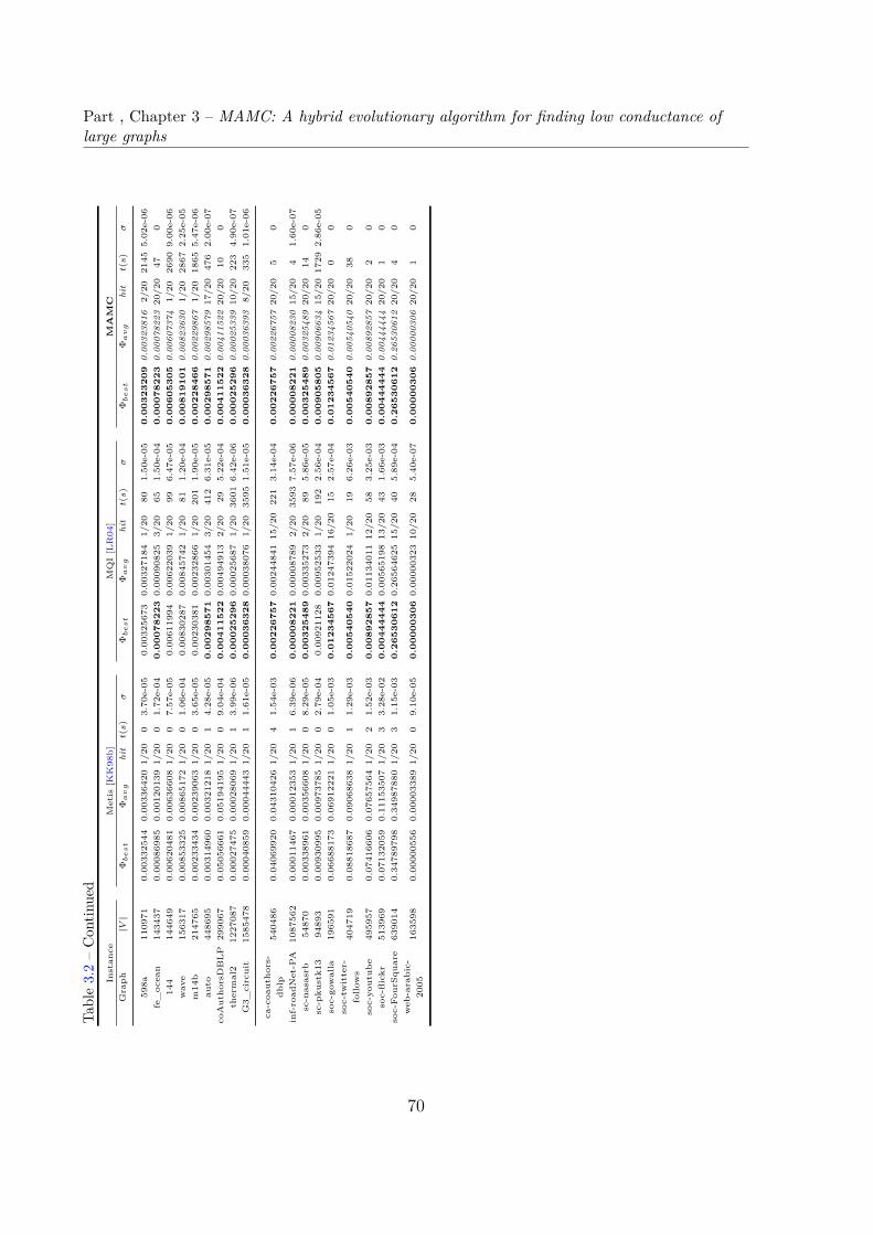
Part , Chapter 3 – MAMC: A hybrid evolutionary algorithm for finding low conductance oflarge graphs
Table3.2–Con
tinued
Instan
ceMetis
[KK98b]
MQI[LR04]
MA
MC
Graph
|V|
Φb
es
tΦ
av
ghi
tt(s)
σΦ
be
st
Φa
vg
hit
t(s)
σΦ
be
st
Φa
vg
hit
t(s)
σ
598a
110971
0.00332544
0.00336420
1/20
03.70e-05
0.00325673
0.00327184
1/20
801.50e-05
0.0
03
23
20
90.
0032
3816
2/20
2145
5.02e-06
fe_ocean
143437
0.00086985
0.00120139
1/20
01.72e-04
0.0
00
78
22
30.00090825
3/20
651.50e-04
0.0
00
78
22
30.
0007
8223
20/20
470
144
144649
0.00620481
0.00636608
1/20
07.57e-05
0.00611994
0.00622039
1/20
996.47e-05
0.0
06
05
30
50.
0060
7374
1/20
2690
9.00e-06
wave
156317
0.00853325
0.00865172
1/20
01.06e-04
0.00830287
0.00845742
1/20
811.20e-04
0.0
08
19
10
10.
0082
3630
1/20
2867
2.25e-05
m14b
214765
0.00233434
0.00239063
1/20
03.65e-05
0.00230381
0.00232866
1/20
201
1.90
e-05
0.0
02
28
46
60.
0022
9867
1/20
1865
5.47e-06
auto
448695
0.00314960
0.00321218
1/20
14.28e-05
0.0
02
98
57
10.00301454
3/20
412
6.31e-05
0.0
02
98
57
10.
0029
8579
17/20
476
2.00e-07
coAutho
rsDBLP
299067
0.05056661
0.05
194195
1/20
09.04e-04
0.0
04
11
52
20.00494913
2/20
295.22e-04
0.0
04
11
52
20.
0041
1522
20/20
100
thermal2
1227087
0.00027475
0.00028069
1/20
13.99e-06
0.0
00
25
29
60.00025687
1/20
3601
6.42e-06
0.0
00
25
29
60.
0002
5339
10/20
223
4.90e-07
G3_
circuit
1585478
0.00040859
0.00044443
1/20
11.61e-05
0.0
00
36
32
80.00038076
1/20
3595
1.51e-05
0.0
00
36
32
80.
0003
6393
8/20
335
1.01e-06
ca-coautho
rs-
dblp
540486
0.04069920
0.04310426
1/20
41.54e-03
0.0
02
26
75
70.00244841
15/20
221
3.14e-04
0.0
02
26
75
70.
0022
6757
20/20
50
inf-road
Net-PA
1087562
0.00011467
0.00012353
1/20
16.39e-06
0.0
00
08
22
10.00008789
2/20
3593
7.57e-06
0.0
00
08
22
10.
0000
8230
15/20
41.60e-07
sc-nasasrb
54870
0.00338961
0.00356608
1/20
08.29e-05
0.0
03
25
48
90.00335273
2/20
895.86e-05
0.0
03
25
48
90.
0032
5489
20/20
140
sc-pku
stk1
394893
0.00930995
0.00973785
1/20
02.79e-04
0.00921128
0.00952533
1/20
192
2.56e-04
0.0
09
05
80
50.
0090
6634
15/201729
2.86e-05
soc-gowalla
196591
0.06688173
0.06912221
1/20
01.05e-03
0.0
12
34
56
70.01247394
16/20
152.57e-04
0.0
12
34
56
70.
0123
4567
20/20
00
soc-tw
itter-
follow
s404719
0.08818687
0.09068638
1/20
11.29e-03
0.0
05
40
54
00.01522024
1/20
196.26e-03
0.0
05
40
54
00.
0054
0540
20/20
380
soc-yo
utub
e495957
0.07416606
0.07657564
1/20
21.52e-03
0.0
08
92
85
70.01134011
12/20
583.25e-03
0.0
08
92
85
70.
0089
2857
20/20
20
soc-flickr
513969
0.07132059
0.11153507
1/20
33.28e-02
0.0
04
44
44
40.00565198
13/20
431.66e-03
0.0
04
44
44
40.
0044
4444
20/20
10
soc-Fou
rSqu
are
639014
0.34789798
0.34987880
1/20
31.15e-03
0.2
65
30
61
20.26564625
15/20
405.89e-04
0.2
65
30
61
20.
2653
0612
20/20
40
web-arabic-
2005
163598
0.00000556
0.00003389
1/20
09.10e-05
0.0
00
00
30
60.00000323
10/20
285.40e-07
0.0
00
00
30
60.
0000
0306
20/20
10
70

3.3. Experimental resultsTa
ble3.3–Detailedcompu
tatio
nalresults
ofMAMC
with
tworeferencestate-of-the-art
algorit
hmsS
aBTS[LHZ1
9]an
dMQI+
SaBT
S[LHZ1
9]on
50largegrap
hsfro
m“T
he10th
DIM
ACSIm
plem
entatio
nCha
lleng
eBe
nchm
ark”
and10
large
grap
hsfro
m“T
heNetwo
rkDataRep
osito
ryon
line”.
Instan
ceSa
BTS[LHZ19]
MQI+
SaBTS[LHZ19]
MA
MC
Graph
|V|
Φb
es
tΦ
av
ghi
tt(s)
σΦ
be
st
Φa
vg
hit
t(s)
σΦ
be
st
Φa
vg
hit
t(s)
σ
preferential
Attachm
ent
100000
0.29468142
0.29575422
1/20
1790
7.22e-04
0.29457883
0.29584725
1/20
2264
1.04e-03
0.2
87
17
31
80.
2880
4940
1/20
2886
6.17e-04
smallworld
100000
0.10048440
0.10
1431
341/20
3191
6.79e-04
0.10105860
0.10387462
1/20
3181
1.99e-03
0.0
99
48
25
90.10321531
1/20
2739
1.27e-03
cnr-2000
325557
0.000144
990.00045286
1/20
179
2.30e-04
0.0
00
00
15
60.00000649
12/20
07.00e-06
0.0
00
00
15
60.
0000
0156
20/20
10
eu-2005
862664
0.00180465
0.00296178
1/20
118
8.54e-04
0.0
00
04
93
00.00064963
5/20
1219
8.75e-04
0.0
00
04
93
00.
0000
4930
20/20
110
road
_central
14081816
0.0
00
01
00
00.00001399
1/20
02.00e-06
0.0
00
01
00
00.00001399
1/20
3240
1.52e-06
0.0
00
01
00
00.
0000
1128
9/20
272
1.21e-06
road
_usa
23947347
0.0
00
00
58
40.00000743
1/20
01.00e-06
0.0
00
00
58
40.00000743
1/20
3420
8.70e-07
0.0
00
00
58
40.
0000
0606
11/20
493
2.80e-07
delaun
ay_n1
665536
0.00244182
0.002545
901/20
05.30e-05
0.00232641
0.00239002
1/20
04.30e-05
0.0
02
26
37
60.
0022
9371
1/20
1292
2.44e-05
delaun
ay_n1
7131072
0.00174222
0.00180321
1/20
03.30e-05
0.00161683
0.00166666
1/20
01.90e-05
0.0
01
56
85
70.
0016
1819
1/20
2000
2.22e-05
delaun
ay_n1
8262144
0.00122711
0.00128230
1/20
482.40e-05
0.00113724
0.00117144
1/20
01.80e-05
0.0
01
13
33
20.
0011
4381
1/20
762
8.03e-06
delaun
ay_n1
9524288
0.00087931
0.00090477
1/20
249
1.80e-05
0.00078757
0.00081717
1/20
471.17e-05
0.0
00
78
69
30.
0008
0017
1/20
729
9.73e-06
delaun
ay_n2
01048576
0.00062085
0.00064504
1/20
651.30e-05
0.0
00
55
89
00.00057389
1/20
997
9.59e-06
0.00055891
0.00
0561
289/20
273.50e-06
delaun
ay_n2
12097152
0.00043742
0.00045553
1/20
448.00e-06
0.0
00
39
29
30.00041812
1/20
1854
3.01e-05
0.0
00
39
29
30.
0003
9397
8/20
451.35e-06
delaun
ay_n2
24194304
0.0
00
31
35
20.00032529
1/20
225
6.00e-06
0.0
00
31
35
20.00032530
1/20
2272
6.42e-06
0.0
00
31
35
20.
0003
1504
13/20
286
2.61e-06
delaun
ay_n2
38388608
0.0
00
22
44
30.00023219
1/20
335
4.00e-06
0.0
00
22
44
30.00023219
1/20
2906
4.08e-06
0.0
00
22
44
30.
0002
2552
8/20
526
1.30e-06
delaun
ay_n2
416777216
0.0
00
16
18
00.00016509
1/20
02.00e-06
0.0
00
16
18
00.00016509
1/20
3420
2.32e-06
0.0
00
16
18
00.
0001
6208
11/201256
3.20e-07
co2010
201062
0.00067382
0.00072937
1/20
03.40e-05
0.00
053700
0.00061060
1/20
05.00e-05
0.0
00
53
44
20.
0005
3453
19/20
564
4.80e-07
la2010
204447
0.00036595
0.00042063
1/20
284.80e-05
0.0
00
17
78
90.00028104
3/20
357.40e-05
0.0
00
17
78
90.
0001
7789
20/20
40
ia2010
216007
0.00067607
0.00071503
1/20
02.50e-05
0.00060102
0.00062450
1/20
01.90e-05
0.0
00
59
14
70.
0006
0046
1/20
1239
4.62e-06
ks2010
238600
0.00057938
0.00063012
1/20
02.40e-05
0.0
00
51
47
00.00054080
1/20
01.60e-05
0.0
00
51
47
00.
0005
1875
10/20
980
4.54e-06
tn2010
240116
0.00043051
0.00048415
1/20
03.00e-05
0.0
00
33
67
10.00038654
8/20
04.10e-05
0.0
00
33
67
10.
0003
3671
20/20
40
az2010
241666
0.00057022
0.00062654
1/20
13.40e-05
0.00
044358
0.00051398
1/20
130
4.10e-05
0.0
00
43
83
90.
0004
5183
1/20
941.90e-05
al2010
252266
0.00057567
0.00065110
1/20
03.70e-05
0.00050982
0.00054469
1/20
692.70e-05
0.0
00
50
73
20.
0005
1154
2/20
1295
4.01e-06
wi2010
253096
0.00053185
0.00062475
1/20
07.30e-05
0.00049099
0.00053505
1/20
106
4.70e-05
0.0
00
48
24
70.
0004
8581
3/20
1374
4.78e-06
mn2
010
259777
0.00061709
0.00066058
1/20
02.30e-05
0.00053535
0.00055552
1/20
161
1.30e-05
0.0
00
53
49
10.
0005
3926
1/20
828
3.59e-06
in2010
267071
0.00054614
0.00060081
1/20
12.70e-05
0.0
00
45
19
90.00047766
7/20
513.20e-05
0.0
00
45
19
90.
0004
5199
20/20
20
ok2010
269118
0.00054185
0.00059924
1/20
13.30e-05
0.00046031
0.00050597
1/20
192
2.10e-05
0.0
00
46
03
00.
0004
6677
2/20
501
9.09e-06
va2010
285762
0.00060130
0.00066431
1/20
13.70e-05
0.0
00
50
62
90.00054526
6/20
129
3.60e-05
0.0
00
50
62
90.
0005
0810
17/20
36.23e-06
nc2010
288987
0.00033045
0.00035826
1/20
12.10e-05
0.00029129
0.00030381
1/20
799.00e-06
0.0
00
29
07
90.
0002
9215
1/20
1218
2.44e-06
ga2010
291086
0.00041692
0.00047249
1/20
744.10e-05
0.00036488
0.00039204
1/20
445
2.30e-05
0.0
00
35
93
50.
0003
6353
1/20
1083
2.93e-06
mi2010
329885
0.00050347
0.00054874
1/20
12.50e-05
0.0
00
09
24
70.00020506
13/20
721.71e-04
0.0
00
09
24
70.
0000
9247
20/20
10
mo2010
343565
0.00054932
0.00061939
1/20
14.60e-05
0.0
00
44
01
00.00050980
1/20
824.20e-05
0.0
00
44
01
00.
0004
4334
13/20
481
1.25e-05
oh2010
365344
0.00055701
0.00059543
1/20
22.20e-05
0.00047052
0.00050873
1/20
116
2.20e-05
0.0
00
45
03
00.
0004
7809
1/20
312
9.88e-06
pa2010
421545
0.00034309
0.00038692
1/20
13.80e-05
0.0
00
26
61
60.00027731
11/20
02.30e-05
0.0
00
26
61
60.
0002
6616
20/20
20
il2010
451554
0.00029324
0.00031372
1/20
11.60e-05
0.00025204
0.00026736
1/20
59.00e-06
0.0
00
24
99
70.
0002
5260
2/20
515
1.74e-06
tx2010
914231
0.00028326
0.00032269
1/20
52.00e-05
0.00024258
0.00025289
1/20
2692
9.51e-06
0.0
00
24
22
10.
0002
4274
2/20
176
4.60e-07
t60k
60005
0.00082876
0.00098630
1/20
91.07e-04
0.0
00
69
38
50.00073344
17/20
69.40e-05
0.0
00
69
38
50.
0006
9385
20/20
10
wing
6203
20.00708296
0.00731614
1/20
01.56e-04
0.00668219
0.00689348
1/20
01.36e-04
0.0
06
54
90
60.
0066
2078
1/20
1953
6.69e-05
brack2
62631
0.0
01
85
33
20.00192248
1/20
1767
4.80e-05
0.0
01
85
33
20.
0018
5332
20/20
70
0.0
01
85
33
20.
0018
5332
20/20
100
fina
n512
74752
0.0
00
62
04
00.
0006
2040
20/20
00
0.0
00
62
04
00.
0006
2040
20/20
00
0.0
00
62
04
00.
0006
2040
20/20
30
fe_tooth
78136
0.00854413
0.00920313
1/20
2008
3.23e-04
0.00857068
0.00893257
1/20
735
2.09e-04
0.0
08
43
14
70.
0084
6699
1/20
2032
8.13e-05
fe_rotor
99617
0.00319580
0.00322448
1/20
2081
2.00e-05
0.00303132
0.00313967
1/20
02.70e-05
0.0
03
02
48
80.
0030
3411
14/20
542
2.59e-05
71
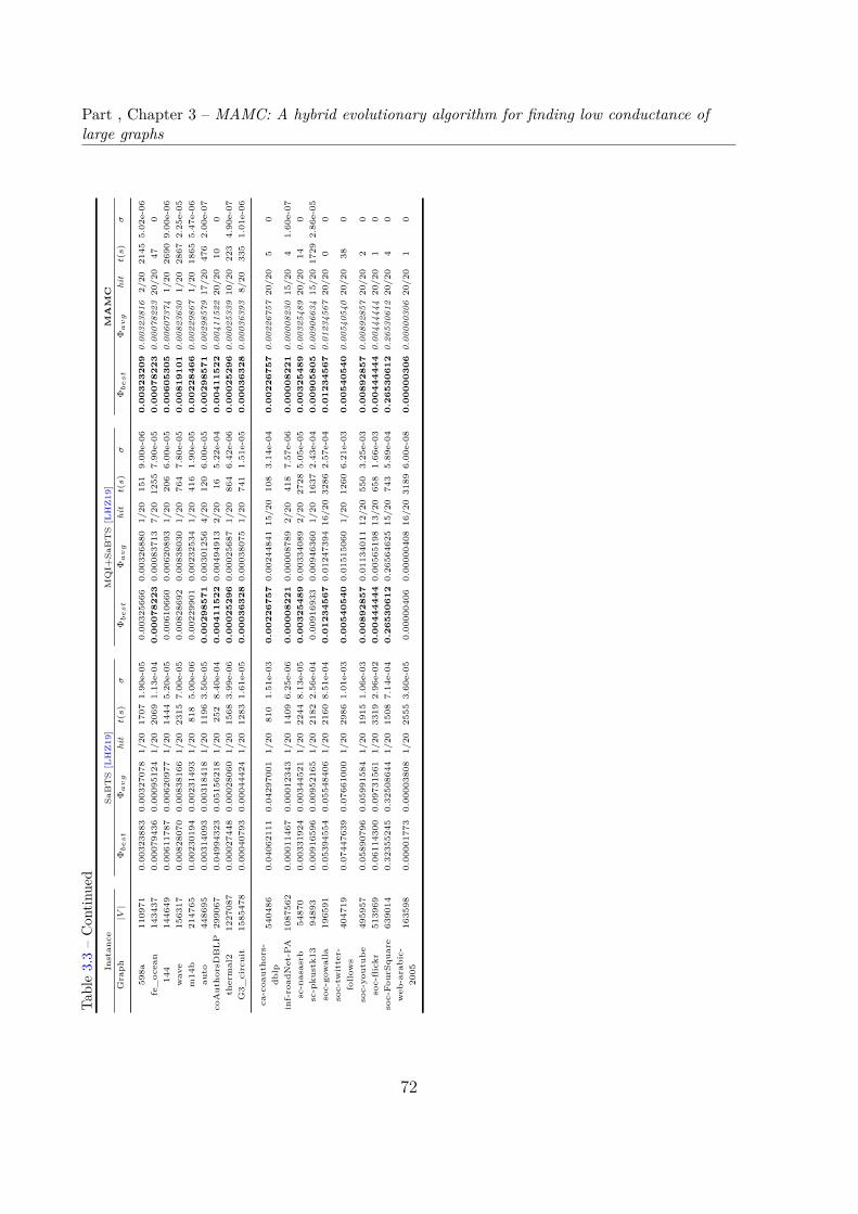
Part , Chapter 3 – MAMC: A hybrid evolutionary algorithm for finding low conductance oflarge graphs
Table3.3–Con
tinued
Instan
ceSa
BTS[LHZ19]
MQI+
SaBTS[LHZ19]
MA
MC
Graph
|V|
Φb
es
tΦ
av
ghi
tt(s)
σΦ
be
st
Φa
vg
hit
t(s)
σΦ
be
st
Φa
vg
hit
t(s)
σ
598a
110971
0.00323883
0.00327078
1/20
1707
1.90e-05
0.00325666
0.00326880
1/20
151
9.00e-06
0.0
03
23
20
90.
0032
3816
2/20
2145
5.02e-06
fe_ocean
143437
0.00079436
0.00095124
1/20
2069
1.13e-04
0.0
00
78
22
30.00083713
7/20
1255
7.90e-05
0.0
00
78
22
30.
0007
8223
20/20
470
144
144649
0.00611787
0.00620977
1/20
1444
5.20e-05
0.00610660
0.00620893
1/20
206
6.00e-05
0.0
06
05
30
50.
0060
7374
1/20
2690
9.00e-06
wave
156317
0.00828070
0.00838166
1/20
2315
7.00e-05
0.00828692
0.00838030
1/20
764
7.80e-05
0.0
08
19
10
10.
0082
3630
1/20
2867
2.25e-05
m14b
214765
0.00230194
0.00231493
1/20
818
5.00e-06
0.00229901
0.00232534
1/20
416
1.90e-05
0.0
02
28
46
60.
0022
9867
1/20
1865
5.47e-06
auto
448695
0.00314093
0.00318418
1/20
1196
3.50e-05
0.0
02
98
57
10.00301256
4/20
120
6.00e-05
0.0
02
98
57
10.
0029
8579
17/20
476
2.00e-07
coAutho
rsDBLP
299067
0.04994323
0.05
156218
1/20
252
8.40e-04
0.0
04
11
52
20.00494913
2/20
165.22e-04
0.0
04
11
52
20.
0041
1522
20/20
100
thermal2
1227087
0.00027448
0.00028060
1/20
1568
3.99e-06
0.0
00
25
29
60.00025687
1/20
864
6.42e-06
0.0
00
25
29
60.
0002
5339
10/20
223
4.90e-07
G3_
circuit
1585478
0.00040793
0.00044424
1/20
1283
1.61e-05
0.0
00
36
32
80.00038075
1/20
741
1.51e-05
0.0
00
36
32
80.
0003
6393
8/20
335
1.01e-06
ca-coautho
rs-
dblp
540486
0.04062111
0.04297001
1/20
810
1.51e-03
0.0
02
26
75
70.00244841
15/20
108
3.14e-04
0.0
02
26
75
70.
0022
6757
20/20
50
inf-road
Net-PA
1087562
0.00011467
0.00012343
1/20
1409
6.25e-06
0.0
00
08
22
10.00008789
2/20
418
7.57e-06
0.0
00
08
22
10.
0000
8230
15/20
41.60e-07
sc-nasasrb
54870
0.00331924
0.00344521
1/20
2244
8.13e-05
0.0
03
25
48
90.00334089
2/20
2728
5.05e-05
0.0
03
25
48
90.
0032
5489
20/20
140
sc-pku
stk1
394893
0.00916596
0.00952165
1/20
2182
2.56e-04
0.009169
330.00946360
1/20
1637
2.43e-04
0.0
09
05
80
50.
0090
6634
15/201729
2.86e-05
soc-gowalla
196591
0.05394554
0.05548406
1/20
2160
8.51e-04
0.0
12
34
56
70.01247394
16/203286
2.57e-04
0.0
12
34
56
70.
0123
4567
20/20
00
soc-tw
itter-
follow
s404719
0.07447639
0.07661000
1/20
2986
1.01e-03
0.0
05
40
54
00.01515060
1/20
1260
6.21e-03
0.0
05
40
54
00.
0054
0540
20/20
380
soc-yo
utub
e495957
0.05890796
0.05991584
1/20
1915
1.06e-03
0.0
08
92
85
70.01134011
12/20
550
3.25e-03
0.0
08
92
85
70.
0089
2857
20/20
20
soc-flickr
513969
0.06114300
0.09731561
1/20
3319
2.96e-02
0.0
04
44
44
40.00565198
13/20
658
1.66e-03
0.0
04
44
44
40.
0044
4444
20/20
10
soc-Fou
rSqu
are
639014
0.32355245
0.32508644
1/20
1508
7.14e-04
0.2
65
30
61
20.26564625
15/20
743
5.89e-04
0.2
65
30
61
20.
2653
0612
20/20
40
web-arabic-
2005
163598
0.00001773
0.00003808
1/20
2555
3.60e-05
0.00000406
0.00000408
16/203189
6.00e-08
0.0
00
00
30
60.
0000
0306
20/20
10
72
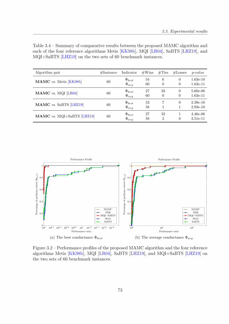
3.3. Experimental results
Table 3.4 – Summary of comparative results between the proposed MAMC algorithm andeach of the four reference algorithms Metis [KK98b], MQI [LR04], SaBTS [LHZ19], andMQI+SaBTS [LHZ19] on the two sets of 60 benchmark instances.
Algorithm pair #Instance Indicator #Wins #Ties #Losses p-value
MAMC vs. Metis [KK98b] 60 Φbest 54 6 0 1.63e-10Φavg 60 0 0 1.63e-11
MAMC vs. MQI [LR04] 60 Φbest 27 33 0 5.60e-06Φavg 60 0 0 1.63e-11
MAMC vs. SaBTS [LHZ19] 60 Φbest 53 7 0 2.39e-10Φavg 58 1 1 2.93e-10
MAMC vs. MQI+SaBTS [LHZ19] 60 Φbest 27 32 1 4.46e-06Φavg 58 2 0 3.51e-11
100 100.2 100.4 100.6 100.8 101 101.2 101.4 101.6 101.80
0.2
0.4
0.6
0.8
1
Performance ratio
Percentag
eof
prob
lemssolved
(Φbest)
Performance Profile
MAMCMQI
MQI+SaBTSMetisSaBTS
(a) The best conductance Φbest
100 101 1020
0.2
0.4
0.6
0.8
1
Performance ratio
Percentag
eof
prob
lemssolved
(Φavg)
Performance Profile
MAMCMQI
MQI+SaBTSMetisSaBTS
(b) The average conductance Φavg
Figure 3.2 – Performance profiles of the proposed MAMC algorithm and the four referencealgorithms Metis [KK98b], MQI [LR04], SaBTS [LHZ19], and MQI+SaBTS [LHZ19] onthe two sets of 60 benchmark instances.
73
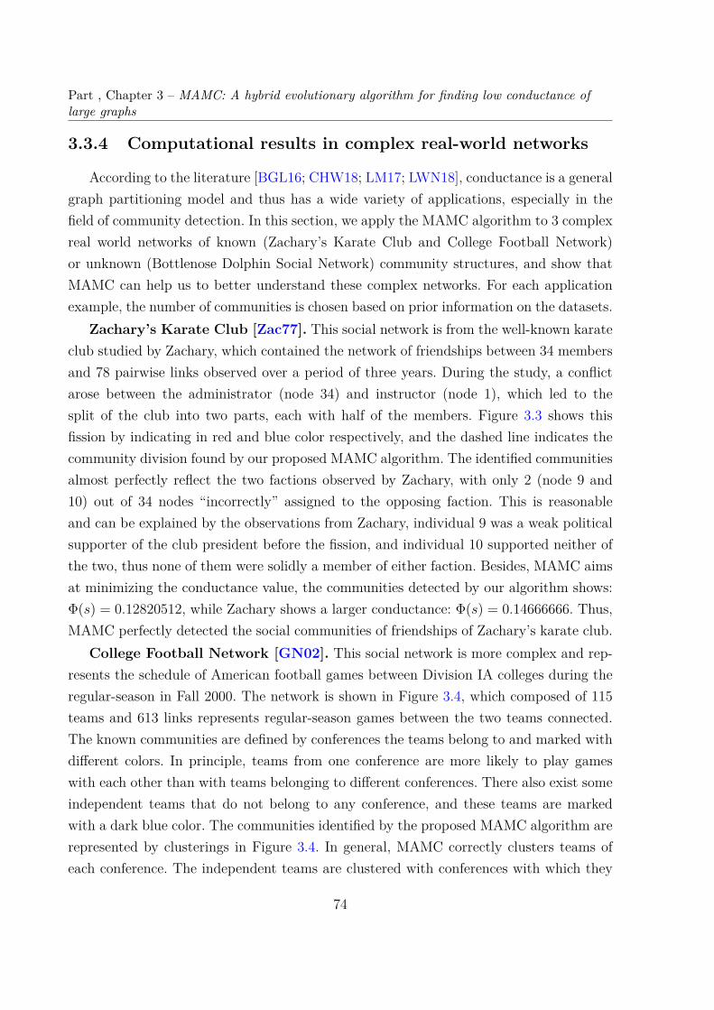
Part , Chapter 3 – MAMC: A hybrid evolutionary algorithm for finding low conductance oflarge graphs
3.3.4 Computational results in complex real-world networks
According to the literature [BGL16; CHW18; LM17; LWN18], conductance is a generalgraph partitioning model and thus has a wide variety of applications, especially in thefield of community detection. In this section, we apply the MAMC algorithm to 3 complexreal world networks of known (Zachary’s Karate Club and College Football Network)or unknown (Bottlenose Dolphin Social Network) community structures, and show thatMAMC can help us to better understand these complex networks. For each applicationexample, the number of communities is chosen based on prior information on the datasets.
Zachary’s Karate Club [Zac77]. This social network is from the well-known karateclub studied by Zachary, which contained the network of friendships between 34 membersand 78 pairwise links observed over a period of three years. During the study, a conflictarose between the administrator (node 34) and instructor (node 1), which led to thesplit of the club into two parts, each with half of the members. Figure 3.3 shows thisfission by indicating in red and blue color respectively, and the dashed line indicates thecommunity division found by our proposed MAMC algorithm. The identified communitiesalmost perfectly reflect the two factions observed by Zachary, with only 2 (node 9 and10) out of 34 nodes “incorrectly” assigned to the opposing faction. This is reasonableand can be explained by the observations from Zachary, individual 9 was a weak politicalsupporter of the club president before the fission, and individual 10 supported neither ofthe two, thus none of them were solidly a member of either faction. Besides, MAMC aimsat minimizing the conductance value, the communities detected by our algorithm shows:Φ(s) = 0.12820512, while Zachary shows a larger conductance: Φ(s) = 0.14666666. Thus,MAMC perfectly detected the social communities of friendships of Zachary’s karate club.
College Football Network [GN02]. This social network is more complex and rep-resents the schedule of American football games between Division IA colleges during theregular-season in Fall 2000. The network is shown in Figure 3.4, which composed of 115teams and 613 links represents regular-season games between the two teams connected.The known communities are defined by conferences the teams belong to and marked withdifferent colors. In principle, teams from one conference are more likely to play gameswith each other than with teams belonging to different conferences. There also exist someindependent teams that do not belong to any conference, and these teams are markedwith a dark blue color. The communities identified by the proposed MAMC algorithm arerepresented by clusterings in Figure 3.4. In general, MAMC correctly clusters teams ofeach conference. The independent teams are clustered with conferences with which they
74
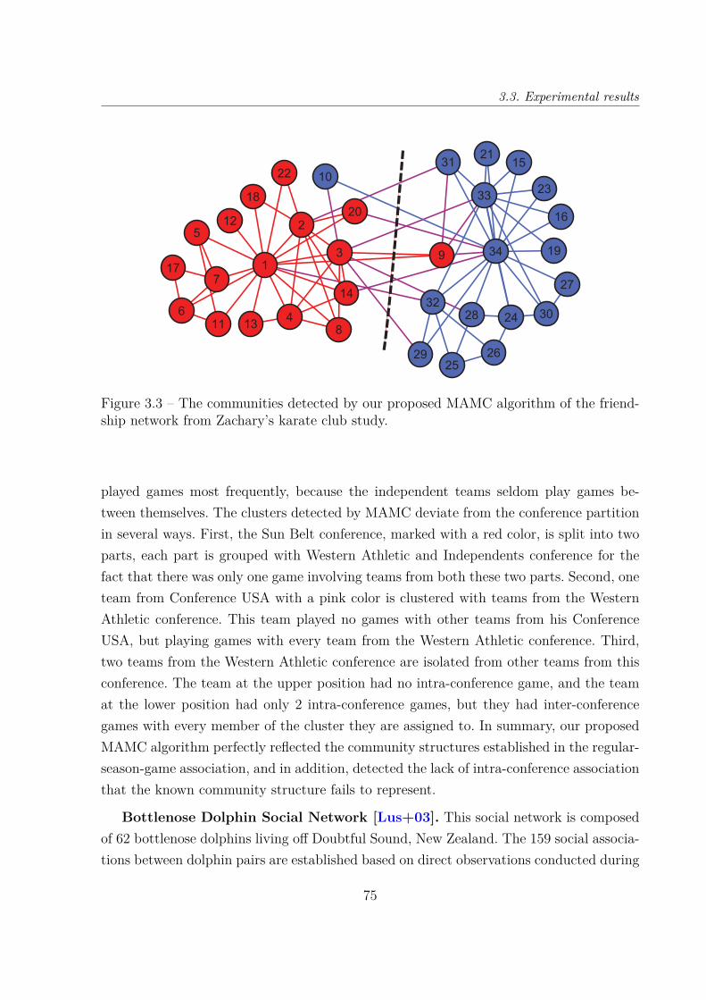
3.3. Experimental results
2
1
3
4
5
6
7
8
9
11
12
13
14
18
20
22
32
31
10
28
29
33
17
34
15
16
19
21
23
26
24 30
25
27
Figure 3.3 – The communities detected by our proposed MAMC algorithm of the friend-ship network from Zachary’s karate club study.
played games most frequently, because the independent teams seldom play games be-tween themselves. The clusters detected by MAMC deviate from the conference partitionin several ways. First, the Sun Belt conference, marked with a red color, is split into twoparts, each part is grouped with Western Athletic and Independents conference for thefact that there was only one game involving teams from both these two parts. Second, oneteam from Conference USA with a pink color is clustered with teams from the WesternAthletic conference. This team played no games with other teams from his ConferenceUSA, but playing games with every team from the Western Athletic conference. Third,two teams from the Western Athletic conference are isolated from other teams from thisconference. The team at the upper position had no intra-conference game, and the teamat the lower position had only 2 intra-conference games, but they had inter-conferencegames with every member of the cluster they are assigned to. In summary, our proposedMAMC algorithm perfectly reflected the community structures established in the regular-season-game association, and in addition, detected the lack of intra-conference associationthat the known community structure fails to represent.
Bottlenose Dolphin Social Network [Lus+03]. This social network is composedof 62 bottlenose dolphins living off Doubtful Sound, New Zealand. The 159 social associa-tions between dolphin pairs are established based on direct observations conducted during
75
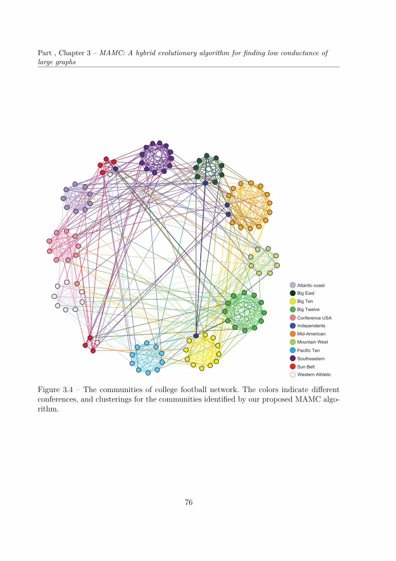
Part , Chapter 3 – MAMC: A hybrid evolutionary algorithm for finding low conductance oflarge graphs
Figure 3.4 – The communities of college football network. The colors indicate differentconferences, and clusterings for the communities identified by our proposed MAMC algo-rithm.
76

3.4. Analysis of MAMC
Fish
Beak
Grin
Haecksel
SN9
SN96
TR77
JetBeescratch
Knit
Notch
Number1 Oscar
SN100
SN90
Upbang
Bumper
Thumper
Zipfel
Double
CCL
Zap
Trigger
Cross
Feather
DN16
Gallatin
WaveWeb
DN21
DN63
PLKringel
SN4
Topless
Ripplefluke
Patchback
Five
Scabs
Fork
Hook
MN83
ShmuddelSN63
Stripes
TR99
TSN103
Jonah
Vau
MN23
Mus
Quasi
MN105
MN60
SMN5
Zig
TR88
SN89
Whitetip
TR120
TSN83
TR82
Figure 3.5 – The social network of 62 bottlenose dolphins. The nodes are colored basedon the groups observed in the study by Lusseau et al [Lus+03]. The clusterings representcommunities detected by our proposed MAMC algorithm.
a period of seven years by Lusseau et al. Figure 3.5 shows the social network of bottlenosedolphins, where nodes represent dolphins and links represent social associations. The 3groups of 40 dolphins observed by Lusseau et al tend to spend more time together thanwith others, are colored in green, red and blue respectively, and the dolphins with yellowcolor are not involved in the clustering analysis. The dashed line denotes the commu-nity division found by our proposed MAMC algorithm. We can see from Figure 3.5, theachieved division corresponds well with the observed groups, separating the red and bluegroups into two communities. The green group is split evenly between the two detectedcommunities, because this group is a weak group and is not well represented by the socialnetwork since most of its members share no social associations [Lus+03].
3.4 Analysis of MAMC
In this section, we first analyze the key parameters of the proposed algorithm, and thenthe impacts of the progressive constrained neighborhood, the pool initialization procedure,and the pool updating procedure.
77
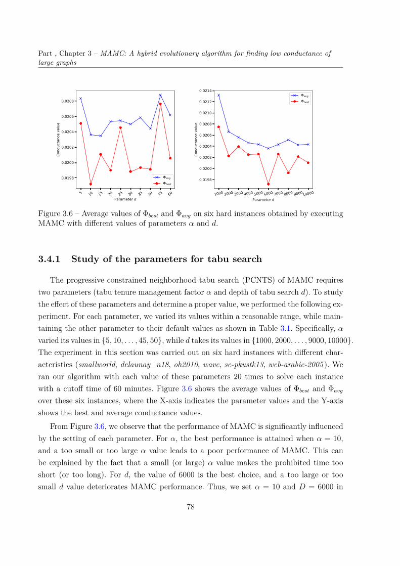
Part , Chapter 3 – MAMC: A hybrid evolutionary algorithm for finding low conductance oflarge graphs
5 10 15 20 25 30 35 40 45 50Parameter
0.0198
0.0200
0.0202
0.0204
0.0206
0.0208
Cond
ucta
nce
valu
e
avg
best
1000 2000 3000 4000 5000 6000 7000 8000 900010000Parameter d
0.0198
0.0200
0.0202
0.0204
0.0206
0.0208
0.0210
0.0212
0.0214
Cond
ucta
nce
valu
e
avg
best
Figure 3.6 – Average values of Φbest and Φavg on six hard instances obtained by executingMAMC with different values of parameters α and d.
3.4.1 Study of the parameters for tabu search
The progressive constrained neighborhood tabu search (PCNTS) of MAMC requirestwo parameters (tabu tenure management factor α and depth of tabu search d). To studythe effect of these parameters and determine a proper value, we performed the following ex-periment. For each parameter, we varied its values within a reasonable range, while main-taining the other parameter to their default values as shown in Table 3.1. Specifically, αvaried its values in 5, 10, . . . , 45, 50, while d takes its values in 1000, 2000, . . . , 9000, 10000.The experiment in this section was carried out on six hard instances with different char-acteristics (smallworld, delaunay_n18, oh2010, wave, sc-pkustk13, web-arabic-2005 ). Weran our algorithm with each value of these parameters 20 times to solve each instancewith a cutoff time of 60 minutes. Figure 3.6 shows the average values of Φbest and Φavg
over these six instances, where the X-axis indicates the parameter values and the Y-axisshows the best and average conductance values.
From Figure 3.6, we observe that the performance of MAMC is significantly influencedby the setting of each parameter. For α, the best performance is attained when α = 10,and a too small or too large α value leads to a poor performance of MAMC. This canbe explained by the fact that a small (or large) α value makes the prohibited time tooshort (or too long). For d, the value of 6000 is the best choice, and a too large or toosmall d value deteriorates MAMC performance. Thus, we set α = 10 and D = 6000 in
78

3.4. Analysis of MAMC
1 2 3 4 5 6 7 8 9 10 11 12 13 14 15Instances
0%
20%
40%
60%
80%
100%
Cond
ucta
nce
gap
(%)
(a) Best resultsInitialRandom1InitialRandom2InitialMixed
1 2 3 4 5 6 7 8 9 10 11 12 13 14 15Instances
0%
20%
40%
60%
80%
100%
Cond
ucta
nce
gap
(%)
(b) Average resultsInitialRandom1InitialRandom2InitialMixed
Figure 3.7 – Comparison of the quality-and-diversity based population initialization (de-noted by InitialMixed) with two random initialization variants (denoted by InitialRan-dom1 and InitialRandom2).
our experiment.
3.4.2 Quality-and-diversity based initialization vs. random ini-tialization
The proposed MAMC algorithm uses a mixed population initialization strategy thattakes into account both quality and diversity (see Section 3.2.2). We study the effect ofthis strategy by comparing it with two random initializations. The first one is a purerandom initialization (denoted by InitialRandom1), while the second one uses the pro-gressive constrained neighborhood tabu search of Section 3.2.4 to improve each randomseeding solution (denoted by InitialRandom2). We tested these two variants within ourMAMC algorithm based on 15 instances arbitrarily chosen from the benchmark set (pref-erentialAttachment, smallworld, cnr-2000, delaunay_n17, delaunay_n18, delaunay_n19,wi2010, ga2010, oh2010, fe_tooth, 144, wave, coAuthorsDBLP, sc-pkustk13, web-arabic-2005 ) and compared the results with the quality-and-diversity based initialization (de-noted by InitialMixed). The plots of their best and average conductance gaps are shownin Figure 3.7, where the X-axis indicates the instances (named by numbers from 1 to 15)and the Y-axis shows the best (or average) conductance gap in percentage. The best (oraverage) conductance gap is calculated as (ΦInitialRandomK−ΦMAMC)/ΦInitialRandomK×100%
79

Part , Chapter 3 – MAMC: A hybrid evolutionary algorithm for finding low conductance oflarge graphs
(K = 1, 2) where ΦInitialRandomK and ΦMAMC are the best (or average) conductance valuesof the variant (InitialRandomK) and MAMC respectively. From Figure 3.7, we observethat MAMC with the quality-and-diversity initialization outperforms the two randominitializations. Moreover, the pure random initialization led to the worst results. Thisexperiment confirms the usefulness of our designed mixed initialization procedure.
3.4.3 Effectiveness of the progressive constrained neighborhood
As described in Section 3.2.4, the proposed MAMC algorithm employs a progres-sive constrained neighborhood in its PCNTS procedure. To assess the usefulness of thisprogressive constrained neighborhood, we created a MAMC variant (denoted by CNTS)where the tabu search procedure of Algorithm 6 examines at each iteration the wholeconstrained neighborhood induced by the whole set of critical vertices CV (s) (i.e., bysetting ev = |CV (s)| in Algorithm 6). To compare MAMC and this variant, we ran bothalgorithm on four selected instances (smallworld, oh2010, wave, sc-pkustk13 ) and showtheir running profiles (convergence graphs) in Figure 3.8.
We observe that thanks to the progressive constrained neighborhood, the MAMCalgorithm has a better convergence throughout the search from the beginning to the endof the given time budget. This holds for all four instances. This experiment confirms therelevance of the adopted progressive constrained neighborhood within the tabu searchbased local optimization procedure.
3.4.4 Effectiveness of the distance-and-quality based pool up-dating procedure
MAMC uses a distance-and-quality based pool updating procedure (see Section 3.2.5)to maintain a healthy population. We present an experiment to assess the effectivenessof this pool updating strategy (denoted by PoolNew) by making a comparison with thetraditional quality based pool updating strategy (denoted by PoolOld) which replaces theworst solution in the population with the offspring solution.
We tested both strategies within our MAMC algorithm based on 15 instances usedin Section 3.4.2. Figure 3.9 provides the plots of their best and average conductancegap. The X-axis indicates the name of instances (named by numbers from 1 to 15).The Y-axis shows the best (or average) conductance gap in percentage, calculated as(ΦPoolOld − ΦMAMC)/ΦPoolOld × 100% where ΦPoolOld is the best (or average) conductance
80
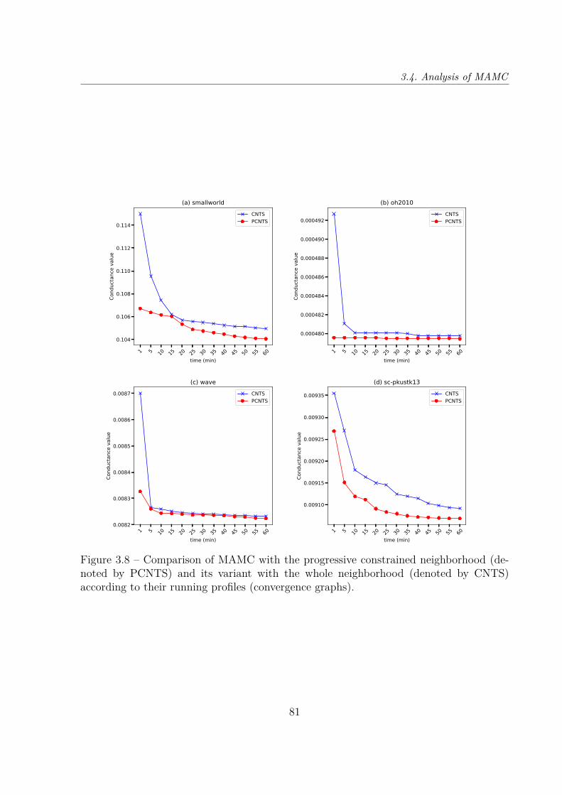
3.4. Analysis of MAMC
1 5 10 15 20 25 30 35 40 45 50 55 60time (min)
0.104
0.106
0.108
0.110
0.112
0.114
Cond
ucta
nce
valu
e
(a) smallworldCNTSPCNTS
1 5 10 15 20 25 30 35 40 45 50 55 60time (min)
0.000480
0.000482
0.000484
0.000486
0.000488
0.000490
0.000492
Cond
ucta
nce
valu
e
(b) oh2010CNTSPCNTS
1 5 10 15 20 25 30 35 40 45 50 55 60time (min)
0.0082
0.0083
0.0084
0.0085
0.0086
0.0087
Cond
ucta
nce
valu
e
(c) waveCNTSPCNTS
1 5 10 15 20 25 30 35 40 45 50 55 60time (min)
0.00910
0.00915
0.00920
0.00925
0.00930
0.00935
Cond
ucta
nce
valu
e
(d) sc-pkustk13CNTSPCNTS
Figure 3.8 – Comparison of MAMC with the progressive constrained neighborhood (de-noted by PCNTS) and its variant with the whole neighborhood (denoted by CNTS)according to their running profiles (convergence graphs).
81
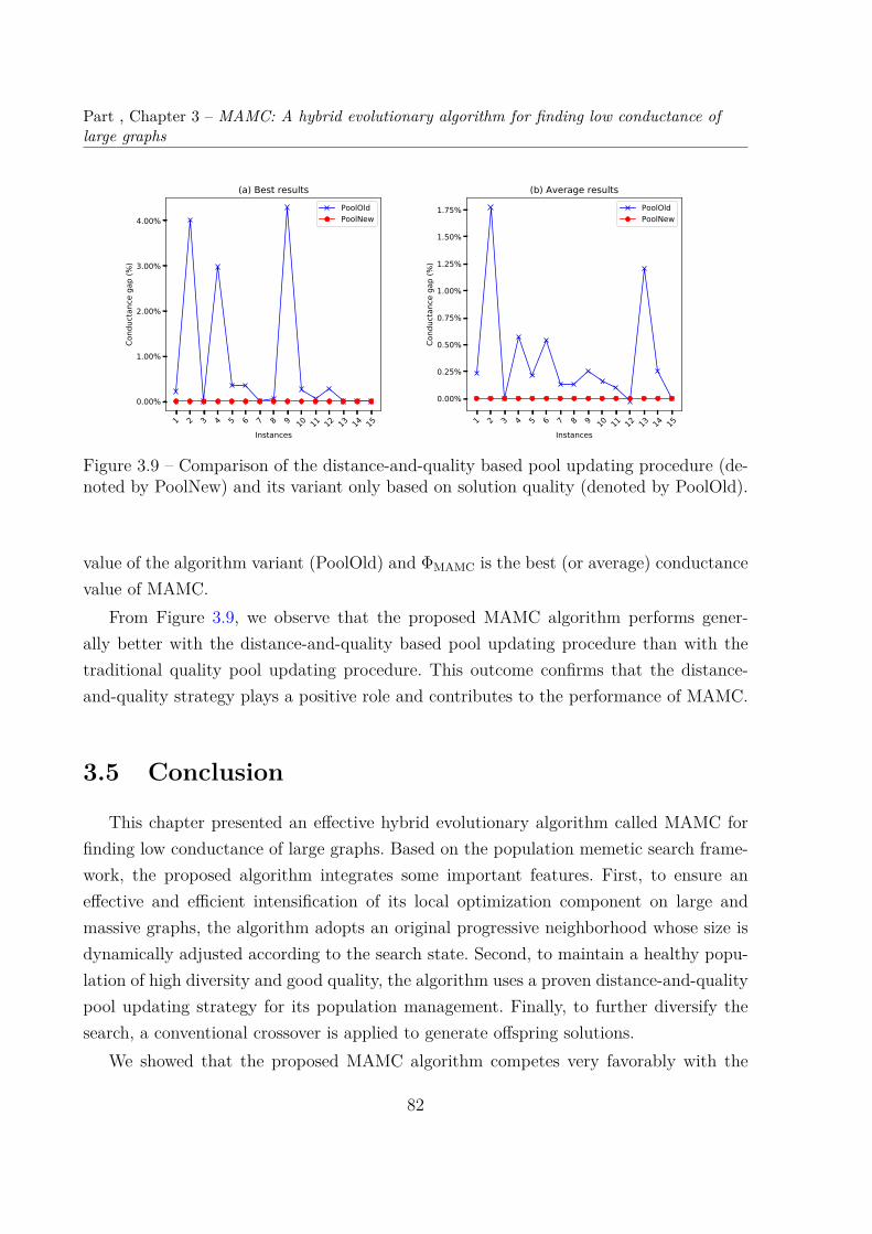
Part , Chapter 3 – MAMC: A hybrid evolutionary algorithm for finding low conductance oflarge graphs
1 2 3 4 5 6 7 8 9 10 11 12 13 14 15Instances
0.00%
1.00%
2.00%
3.00%
4.00%
Cond
ucta
nce
gap
(%)
(a) Best resultsPoolOldPoolNew
1 2 3 4 5 6 7 8 9 10 11 12 13 14 15Instances
0.00%
0.25%
0.50%
0.75%
1.00%
1.25%
1.50%
1.75%
Cond
ucta
nce
gap
(%)
(b) Average resultsPoolOldPoolNew
Figure 3.9 – Comparison of the distance-and-quality based pool updating procedure (de-noted by PoolNew) and its variant only based on solution quality (denoted by PoolOld).
value of the algorithm variant (PoolOld) and ΦMAMC is the best (or average) conductancevalue of MAMC.
From Figure 3.9, we observe that the proposed MAMC algorithm performs gener-ally better with the distance-and-quality based pool updating procedure than with thetraditional quality pool updating procedure. This outcome confirms that the distance-and-quality strategy plays a positive role and contributes to the performance of MAMC.
3.5 Conclusion
This chapter presented an effective hybrid evolutionary algorithm called MAMC forfinding low conductance of large graphs. Based on the population memetic search frame-work, the proposed algorithm integrates some important features. First, to ensure aneffective and efficient intensification of its local optimization component on large andmassive graphs, the algorithm adopts an original progressive neighborhood whose size isdynamically adjusted according to the search state. Second, to maintain a healthy popu-lation of high diversity and good quality, the algorithm uses a proven distance-and-qualitypool updating strategy for its population management. Finally, to further diversify thesearch, a conventional crossover is applied to generate offspring solutions.
We showed that the proposed MAMC algorithm competes very favorably with the
82
3.5. Conclusion
current best performing algorithms when it is assessed on 60 large-scale real world bench-mark instances, including 50 graphs from the 10th DIMACS Implementation ChallengeBenchmark and 10 graphs from the Network Data Repository online, with up to 23 millionvertices. Computational results led to the main conclusions that 1) our algorithm domi-nates the reference algorithms for the tested instances, and 2) it is able to further improvethe solutions obtained by the popular max-flow quotient-cut improvement algorithm MQI[LR04]. As an application example, we showed the proposed MAMC algorithm can be usedto detect meaningful community structures in complex networks. Finally, we investigatedthe essential components of the proposed MAMC algorithm, leading to the findings that 1)the progressive neighborhood used by the local optimization procedure plays an importantrole of ensuring a fast convergence of the algorithm, and 2) the quality-and-diversity poolinitialization and distance-and-quality pool management help the algorithm to maintaina healthy population, which contributes to its performance.
83

Chapter 4
IMSA: ITERATED MULTILEVEL
SIMULATED ANNEALING FOR
LARGE-SCALE GRAPH CONDUCTANCE
MINIMIZATION
4.1 Introduction
In this chapter, we investigate the multilevel approach for tackling MC-GPP. Throughour researches on MC-GPP, we observe that the existing approaches still have difficultiesin robustly and consistently producing high-quality solutions for large-scale graphs andmay require a substantial amount of computation time to reach the reported results. Onthe other hand, it is known that multilevel approach is a powerful and general frameworkfor large graph partitioning [BS94; BH11a; BJ93; HL95; Val+20; Wal04]. To the best of ourknowledge, this approach has not been investigated for solving MC-GPP. Thus, this workfills this gap by presenting the first multilevel algorithm for the minimum conductancegraph partitioning problem. We summarize the work as follows.
— First, we present an iterated multilevel simulated annealing algorithm (IMSA) forMC-GPP consisting of an original solution-guided coarsening method and a pow-erful local refinement procedure based on a constrained neighborhood to effectivelysample the search space of the problem.
— Second, we perform extensive computational assessments on two sets of 66 very largereal-world benchmark instances (including 56 graphs from the 10th DIMACS Imple-mentation Challenge Benchmark and 10 graphs from the Network Data Repositoryonline, with up to 23 million vertices). The computational experiments indicate ahigh competitiveness of the proposed IMSA algorithm compared to existing state-
85
Part , Chapter 4 – IMSA: Iterated multilevel simulated annealing for large-scale graphconductance minimization
of-the-art algorithms, reporting new record-breaking results for 41 of the testedgraphs.
— Third, we make the code of our IMSA algorithm publicly available, which can helpresearchers and practitioners to better solve various practical problems that can beformulated as MC-GPP.
The chapter is organized as follows. Section 4.2 presents the proposed IMSA algorithm.Section 4.3 shows the computational studies and comparisons between the proposed IMSAalgorithm and the state-of-the-art algorithms. Section 4.4 provides analyses of the keyalgorithmic components. Section 4.5 presents concluding remarks.
4.2 Iterated multilevel simulated annealing for large-scale graph conductance minimization
This section presents the proposed iterated multilevel simulated annealing algorithm(IMSA) for MC-GPP. We first show the general framework of IMSA, followed by detaileddescriptions of the key algorithmic components in the subsequent sections.
4.2.1 General outline
The multilevel approach is a general framework that has shown to be very successfulin tackling the classic graph partitioning problem [BS94; BH11a; BJ93; HL95; Val+20;Wal04]. Generally, this approach consists of three basic phases (coarsening, initial par-titioning, and uncoarsening) [HL95]. During the coarsening phase, the given graph issuccessively reduced to obtain a series of coarsened graphs with a decreasing number ofvertices. An initial partition is then generated for the coarsest graph. Finally, during theuncoarsening phase, the coarsened graphs are successively unfolded in the reverse order ofthe coarsening phase. For each uncoarsened graph, the partition of the underlying coars-ened graph is projected back to the uncoarsened graph and then improved by a refinementprocedure. This process stops when the input graph is recovered and its partition is re-fined. In [Wal04], Walshaw introduced iterated multilevel partitioning (analogous to theuse of V-cycles in multigrid methods [TOS01]) where the coarsening-uncoarsening processis iterated and the partition of the current iteration is used for the whole coarsening phaseof the next iteration.
86

4.2. Iterated multilevel simulated annealing for large-scale graph conductance minimization
Algorithm 8 Main framework of the iterated multilevel simulated annealing (IMSA) forMC-GPP.Require: Graph G = (V,E), seeding partition s0, coarsening threshold ct.Ensure: The best partition s∗ found during the search.1: s∗ ← s02: i← 03: repeat4: while |Vi| > ct do5: (Gi+1, si+1)← Solution_Guided_Coarsening(Gi, si) /∗ Section 4.2.2 ∗/6: si+1 ← Local_Refinement(si+1) /∗ Sections 4.2.4 and 4.2.5 ∗/7: i← i+ 18: end while9: while i > 0 do
10: i← i− 111: (Gi, si)← Uncoarsening(Gi+1, si+1) /∗ Section 4.2.3 ∗/12: si ← Local_Refinement(si)13: end while14: if Φ(si) < Φ(s∗) then15: s∗ ← si16: end if17: until Stopping condition is met18: return s∗
Based on the ideas described above, we propose in this work an iterated multilevelsimulated annealing algorithm (IMSA) for MC-GPP, which distinguishes itself by twooriginal features: 1) a solution-guided coarsening method, and 2) a powerful refinementprocedure which is applied during both the coarsening and the uncoarsening phase. Fig.4.1 illustrates the iterated multilevel framework adopted by the proposed IMSA algorithm,while the entire algorithmic framework is presented in Algorithm 8. Informally, IMSAperforms a series of V-cycles, where each V-cycle is composed of a coarsening phase andan uncoarsening phase, mixed with local refinement for each intermediate (coarsened anduncoarsened) graph.
It is worth noting that IMSA requires a seeding partition s0 of the input graph to initi-ate its first iteration (the first V-cycle). Generally, the seeding partition can be provided byany means. For instance, for our experimental studies reported in Section 4.3, we adoptedthe (fast) MQI algorithm [LR04]. For each subsequent iteration, the best partition foundduring the previous V-cycle then serves as the new seeding partition. The whole processterminates when a given stopping condition (e.g., cutoff time limit, maximum number ofV-cycles) is reached and the global best partition found during the search is returned.
87
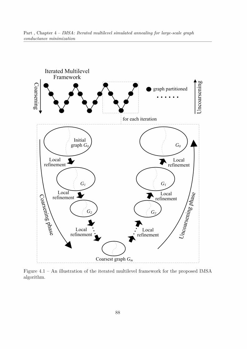
Part , Chapter 4 – IMSA: Iterated multilevel simulated annealing for large-scale graphconductance minimization
graph partitioned
Local refinement
Local refinement
Local refinement
Local refinement
Local refinement
Local refinement
Initial graph G0 G0
G1 G1
G2G2
Coarsest graph Gm
for each iteration
Figure 4.1 – An illustration of the iterated multilevel framework for the proposed IMSAalgorithm.
88
4.2. Iterated multilevel simulated annealing for large-scale graph conductance minimization
4.2.2 Solution-guided coarsening procedure
Given a graph G = (V,E) (renamed as G0 = (V0, E0)) and the seeding partition s0, thesolution-guided coarsening phase progressively transforms G0 into smaller intermediategraphs Gi = (Vi, Ei) such that |Vi| > |Vi+1| (i = 0, . . . ,m − 1), until the last coarsenedgraph Gm becomes sufficiently small (i.e., the number of vertices in Vm is below a giventhreshold ct). During the coarsening process, all intermediate graphs are recorded for thepurpose of uncoarsening.
Generally, to generate a coarsened graphGi+1 fromGi, the coarsening process performstwo consecutive steps: an edge matching step and an edge contraction step.
The edge matching step aims to find an independent set of edges M ⊂ Ei such thatthe endpoints of any two edges inM are not adjacent. For this purpose, IMSA adopts thefast Heavy-Edge Matching (HEM) heuristic [KK98a] with a time complexity of O(|E|).HEM considers vertices in a random order, and matches each unmatched vertex v with itsunmatched neighbor vertex u such that 1) v and u are in the same subset of the currentpartition si; and 2) edge (v, u) has the maximum weight over all edges incident to v. Inour case, edge matching is guided by the current partition si of Gi in the sense that thecut edges in the cut-set cut(si) are ignored and only vertices of the same partition subsetare considered for matching.
The edge contraction step collapses the endpoints of each edge (va, vb) in M to forma new vertex va + vb in the coarsened graph Gi+1, while vertices which are not endpointsof any edge of M are simply copied over to Gi+1. For the new vertex va + vb ∈ Vi+1, itsweight is set to be the sum of the weights of va and vb. The edge between va and vb isremoved, and the edges incident to va and vb are merged to form a new edge in Ei+1 witha weight that is set to the sum of the weights of the merged edges.
Once the coarsened graph Gi+1 is created, the partition si of Gi is projected to Gi+1,followed by improvement with the local refinement procedure. The improved partition isthen used to create the next coarsened graph.
Fig. 4.2 illustrates how the first coarsened graph is created from an initial graphG0 with 8 vertices (unit weight for both vertices and edges) and the partition s0 =(a, b, h, c, d, e, f, g) (indicated by the red dashed line). The edge matching step firstuses the HEM heuristic to identify the set of independent edges M = (a, b), (c, d), (e, f)guided by s0. Then for each edge in M , say (a, b), its endpoints are merged to form a newvertex a+ b in G1 with vertex weight w(a+ b) = w(a) +w(b), the edge (a, b) is removed,and the edges (a, h) and (b, h) which are incident to both a and b are merged to form a
89
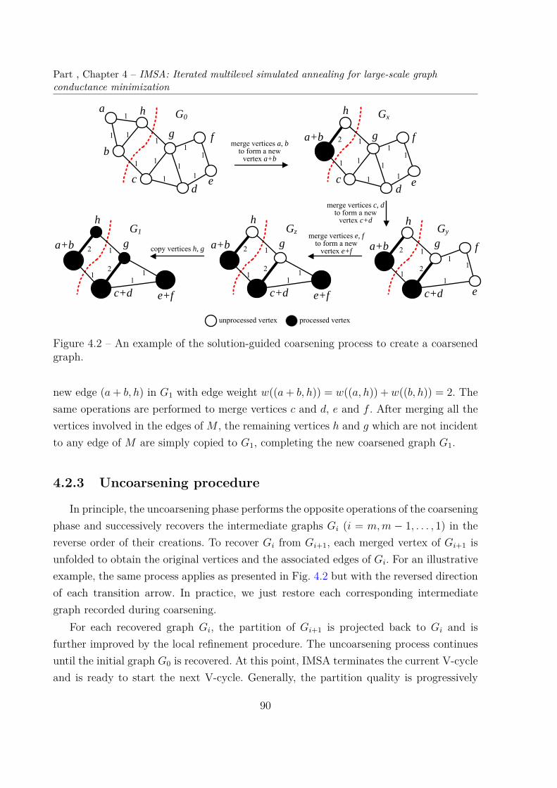
Part , Chapter 4 – IMSA: Iterated multilevel simulated annealing for large-scale graphconductance minimization
a
b
e
h
g f
dc
11
111
1
1 1
11
1
G0
merge vertices a, bto form a new
vertex a+b
a+b
e
h
g f
dc
2
1
1
11
1
11
1
Gx
a+b
e
h
g f
c+d
2
2
1
1
11
1
Gy
a+b
e+f
h
g
c+d
2
2
11
1
1
G1 merge vertices e, fto form a new
vertex e+fcopy vertices h, g
merge vertices c, dto form a new
vertex c+d
a+b
e+f
h
g
c+d
2
2
11
1
1
Gz
processed vertexunprocessed vertex
Figure 4.2 – An example of the solution-guided coarsening process to create a coarsenedgraph.
new edge (a+ b, h) in G1 with edge weight w((a+ b, h)) = w((a, h)) +w((b, h)) = 2. Thesame operations are performed to merge vertices c and d, e and f . After merging all thevertices involved in the edges of M , the remaining vertices h and g which are not incidentto any edge of M are simply copied to G1, completing the new coarsened graph G1.
4.2.3 Uncoarsening procedure
In principle, the uncoarsening phase performs the opposite operations of the coarseningphase and successively recovers the intermediate graphs Gi (i = m,m − 1, . . . , 1) in thereverse order of their creations. To recover Gi from Gi+1, each merged vertex of Gi+1 isunfolded to obtain the original vertices and the associated edges of Gi. For an illustrativeexample, the same process applies as presented in Fig. 4.2 but with the reversed directionof each transition arrow. In practice, we just restore each corresponding intermediategraph recorded during coarsening.
For each recovered graph Gi, the partition of Gi+1 is projected back to Gi and isfurther improved by the local refinement procedure. The uncoarsening process continuesuntil the initial graph G0 is recovered. At this point, IMSA terminates the current V-cycleand is ready to start the next V-cycle. Generally, the partition quality is progressively
90
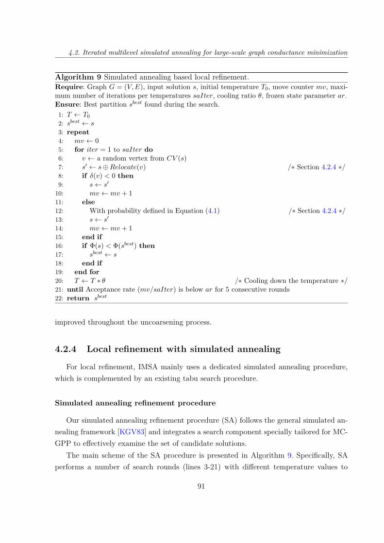
4.2. Iterated multilevel simulated annealing for large-scale graph conductance minimization
Algorithm 9 Simulated annealing based local refinement.Require: Graph G = (V,E), input solution s, initial temperature T0, move counter mv, maxi-mum number of iterations per temperatures saIter, cooling ratio θ, frozen state parameter ar.Ensure: Best partition sbest found during the search.1: T ← T02: sbest ← s3: repeat4: mv ← 05: for iter = 1 to saIter do6: v ← a random vertex from CV (s)7: s′ ← s⊕Relocate(v) /∗ Section 4.2.4 ∗/8: if δ(v) < 0 then9: s← s′
10: mv ← mv + 111: else12: With probability defined in Equation (4.1) /∗ Section 4.2.4 ∗/13: s← s′
14: mv ← mv + 115: end if16: if Φ(s) < Φ(sbest) then17: sbest ← s18: end if19: end for20: T ← T ∗ θ /∗ Cooling down the temperature ∗/21: until Acceptance rate (mv/saIter) is below ar for 5 consecutive rounds22: return sbest
improved throughout the uncoarsening process.
4.2.4 Local refinement with simulated annealing
For local refinement, IMSA mainly uses a dedicated simulated annealing procedure,which is complemented by an existing tabu search procedure.
Simulated annealing refinement procedure
Our simulated annealing refinement procedure (SA) follows the general simulated an-nealing framework [KGV83] and integrates a search component specially tailored for MC-GPP to effectively examine the set of candidate solutions.
The main scheme of the SA procedure is presented in Algorithm 9. Specifically, SAperforms a number of search rounds (lines 3-21) with different temperature values to
91
Part , Chapter 4 – IMSA: Iterated multilevel simulated annealing for large-scale graphconductance minimization
improve the current solution s (i.e., a cut (S, S)). At the start of each search round, themove counter mv is initialized to 0 (line 4). The procedure enters the ‘for’ loop to carryout saIter iterations (saIter is a parameter) with the current temperature T (initiallyset to T0). At each iteration, SA randomly samples a neighbor solution s′ of s from aset of constrained candidates (lines 5-19). This is achieved by displacing a random vertexfrom the set of critical vertices CV (s) (see Section 4.2.4) from its current subset to theopposite subset (lines 6-7, where s′ ← s⊕Relocate(v) denotes this move operation). Thenew solution s′ then replaces the current solution s according to the following probability(lines 8-15),
Prs← s′ =
1 , if δ < 0e−δ/T , if δ ≥ 0
(4.1)
where δ = Φ(s′) − Φ(s) is the conductance variation (also called the move gain) oftransitioning from s to s′.
A better neighbor solution s′ in terms of the conductance (δ < 0) is always accepted asthe new current solution s. Otherwise (δ ≥ 0), the transition from s to s′ takes place withprobability e−δ/T . After each solution transition, the move counter mv is incremented by1. The best solution sbest is updated each time a better solution is found (lines 16-18).Once the number of sampled solutions reaches saIter, the temperature T is cooled downby a constant factor θ ∈ [0, 1] (θ is a parameter, line 20), and SA proceeds to the nextsearch round with this lowered new temperature. The termination criterion (the frozenstate) of SA is met when the acceptance rate becomes smaller than a threshold ar (aris a parameter) for 5 consecutive search rounds, where the acceptance rate is defined asmv/saIter (line 21). Upon the termination of the SA procedure, the procedure returnsthe best recorded solution sbest (line 22).
One critical issue in the SA procedure concerns the initial temperature T0. While ahigh T0 leads to acceptance of many deteriorating uphill moves, a low initial temperaturewill have the same impact as a pure descent procedure resulting in the search to easilybecome trapped in a local optimum. To identify a suitable initial temperature, we use asimple binary search to provide a tradeoff between these two extremes. Given an initialtemperature range T ∈ [1.0e-20, 1.0], T0 is initialized with the median value from thisrange, i.e., T0 = (1.0 + 1.0e-20)/2. If the last round of the search using the current valueof T0 resulted in an acceptance rate of 50%, the value of T0 is left unchanged. Otherwise,the value for T0 used in next round of the search is set to the median value of the upper
92

4.2. Iterated multilevel simulated annealing for large-scale graph conductance minimization
or the lower temperature range depending on whether the acceptance rate is higher orlower than 50%. This process continues until a suitable initial temperature T0 is found fora given problem instance. We investigate the other parameters (saIter, θ, and ar) of SAin Section 4.4.4.
Solution sampling with critical vertices
To generate a new candidate solution s′ from the current solution s, we apply thepopular Relocate operator that displaces a vertex from its current set to the oppositeset. To avoid the generation of non-promising candidate solutions, we identify the set ofcritical vertices with respect to the current solution s.
To ensure a fast computation of the conductance variation of a neighbor solution gen-erated by Relocate, we adopt a streamlined incremental evaluation technique [Cha17;LHW20; LHZ19]. Let s = S, S be the current solution, s′ = S ′, S ′ be the neigh-bor solution after relocating vertex v of s from S to S. The conductance of s′ canbe evaluated in O(1) time by simply updating |cut(s′)|, vol(S ′), vol(S ′) by |cut(s′)| =|cut(s)| + degS(v) − degS(v), vol(S ′) = vol(S) − deg(v), and vol(S ′) = vol(S) + deg(v),where degS(v) (resp. degS(v)) is the number of vertices adjacent to v in S (resp. in S).Moreover, for each vertex w adjacent to v, degS′(w) and degS′(w) can be updated in O(1)time by degS′(w) = degS(w)− 1 and degS′(w) = degS(w) + 1.
We now analyze the complexity of the SA procedure. In each search round of SA, weperform saIter iterations. At each iteration, SA first identifies the set of critical verticesCV (s), which can be achieved in O(|V | × degmax) time where degmax is the maximumdegree of vertex of a given graph G. A candidate solution is then sampled in O(1) time.When a neighbor solution s′ = S ′, S ′ is obtained, the conductance variation is calculatedin O(1) time. Moreover, degS′(w) and degS′(w) are updated in O(deg(v)) time. Thus, foreach search round, SA requires O(saIter × |V | × degmax) time.
4.2.5 Additional solution refinement with tabu search
To further reinforce the solution refinement, we additionally apply the constrainedneighborhood tabu search (CNTS) procedure which is the main component of the SaBTSalgorithm introduced in [LHZ19]. CNTS relies on the same constrained neighborhooddefined by the critical vertices and employs a dynamic tabu list management technique.CNTS requires two parameters: the depth of tabu search D, and the tabu tenure man-
93
Part , Chapter 4 – IMSA: Iterated multilevel simulated annealing for large-scale graphconductance minimization
agement factor α. Section 4.4.4 explains the procedure used to tune these parameters andshows and analyzes their sensitivity. More details about CNTS can be found in [LHZ19].The use of CNTS is based on our preliminary observation that it can provide performancegains especially for the class of relatively small-sized instances such as ‘xx2010’ (see Sec-tion 4.3.2, Table 4.2). Generally, the CNTS component can be safely disabled for largegraphs without impacting the performance of the IMSA algorithm. In terms of solutionrefinement, CNTS plays a complementary and secondary role compared to the SA pro-cedure. In practice, CNTS performs a much shorter search (determined by the depth oftabu search) than SA during a round of IMSA.
4.3 Experimental results
To assess the overall performance of the proposed IMSA algorithm, we test it on atotal of 66 very-large benchmark instances with 54,870 to 23,947,347 vertices. The first56 instances are very large graphs from The 10th DIMACS Implementation ChallengeBenchmark 1, which were introduced for graph partitioning and graph clustering [Bad+14;Bad+13]. The remaining 10 instances are large real world network graphs [RA15] fromThe Network Data Repository online 2. Among these 66 instances, 29 DIMACS graphs andthe 10 massive network graphs have previously been used for experimental evaluations in[LHW20]. We considered the additional 27 large-scale DIMACS benchmark graphs (with114,599 to 21,198,119 vertices) to better assess the scalability of our multilevel algorithm.
4.3.1 Experimental setting and reference algorithms
The proposed IMSA algorithm was implemented in C++ 3 and compiled using theg++ compiler with the “-O3” option. All the experiments were conducted on an AMDOpteron 4184 processor (2.80GHz) with 32GB RAM under Linux operating system.
To evaluate the performance of IMSA, we conduct comparisons with three state-of-the-art MC-GPP algorithms from the literature: 1) the hybrid evolutionary algorithmMAMC [LHW20], 2) the breakout local search algorithm SaBTS [LHZ19], and 3) themax-flow algorithm MQI [LR04]. To the best of our knowledge, MAMC is the current
1. https://www.cc.gatech.edu/dimacs10/downloads.shtml2. http://networkrepository.com/index.php3. The code of the IMSA algorithm will be made publicly available at: http://www.info.
univ-angers.fr/pub/hao/IMSA.html
94
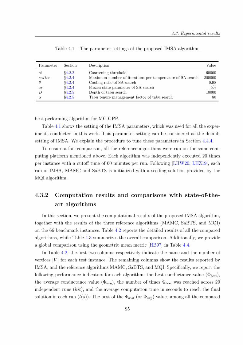
4.3. Experimental results
Table 4.1 – The parameter settings of the proposed IMSA algorithm.
Parameter Section Description Value
ct §4.2.2 Coarsening threshold 60000saIter §4.2.4 Maximum number of iterations per temperature of SA search 200000θ §4.2.4 Cooling ratio of SA search 0.98ar §4.2.4 Frozen state parameter of SA search 5%D §4.2.5 Depth of tabu search 10000α §4.2.5 Tabu tenure management factor of tabu search 80
best performing algorithm for MC-GPP.Table 4.1 shows the setting of the IMSA parameters, which was used for all the exper-
iments conducted in this work. This parameter setting can be considered as the defaultsetting of IMSA. We explain the procedure to tune these parameters in Section 4.4.4.
To ensure a fair comparison, all the reference algorithms were run on the same com-puting platform mentioned above. Each algorithm was independently executed 20 timesper instance with a cutoff time of 60 minutes per run. Following [LHW20; LHZ19], eachrun of IMSA, MAMC and SaBTS is initialized with a seeding solution provided by theMQI algorithm.
4.3.2 Computation results and comparisons with state-of-the-art algorithms
In this section, we present the computational results of the proposed IMSA algorithm,together with the results of the three reference algorithms (MAMC, SaBTS, and MQI)on the 66 benchmark instances. Table 4.2 reports the detailed results of all the comparedalgorithms, while Table 4.3 summarizes the overall comparison. Additionally, we providea global comparison using the geometric mean metric [HB97] in Table 4.4.
In Table 4.2, the first two columns respectively indicate the name and the number ofvertices |V | for each test instance. The remaining columns show the results reported byIMSA, and the reference algorithms MAMC, SaBTS, and MQI. Specifically, we report thefollowing performance indicators for each algorithm: the best conductance value (Φbest),the average conductance value (Φavg), the number of times Φbest was reached across 20independent runs (hit), and the average computation time in seconds to reach the finalsolution in each run (t(s)). The best of the Φbest (or Φavg) values among all the compared
95
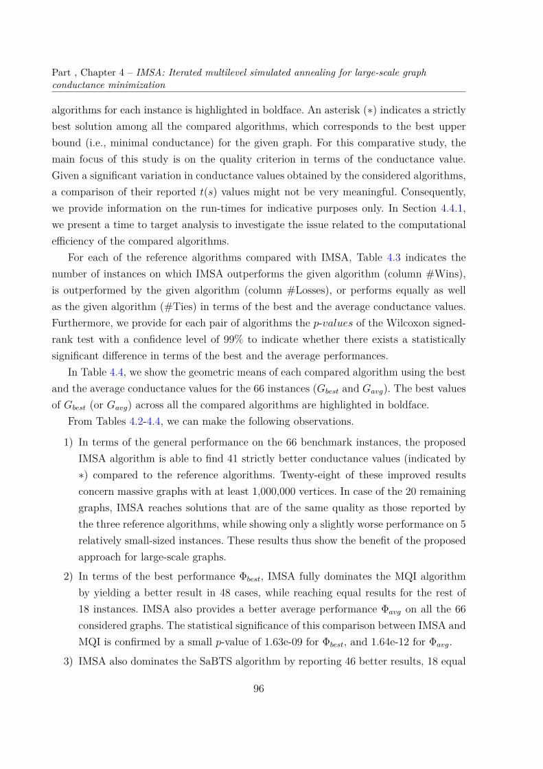
Part , Chapter 4 – IMSA: Iterated multilevel simulated annealing for large-scale graphconductance minimization
algorithms for each instance is highlighted in boldface. An asterisk (∗) indicates a strictlybest solution among all the compared algorithms, which corresponds to the best upperbound (i.e., minimal conductance) for the given graph. For this comparative study, themain focus of this study is on the quality criterion in terms of the conductance value.Given a significant variation in conductance values obtained by the considered algorithms,a comparison of their reported t(s) values might not be very meaningful. Consequently,we provide information on the run-times for indicative purposes only. In Section 4.4.1,we present a time to target analysis to investigate the issue related to the computationalefficiency of the compared algorithms.
For each of the reference algorithms compared with IMSA, Table 4.3 indicates thenumber of instances on which IMSA outperforms the given algorithm (column #Wins),is outperformed by the given algorithm (column #Losses), or performs equally as wellas the given algorithm (#Ties) in terms of the best and the average conductance values.Furthermore, we provide for each pair of algorithms the p-values of the Wilcoxon signed-rank test with a confidence level of 99% to indicate whether there exists a statisticallysignificant difference in terms of the best and the average performances.
In Table 4.4, we show the geometric means of each compared algorithm using the bestand the average conductance values for the 66 instances (Gbest and Gavg). The best valuesof Gbest (or Gavg) across all the compared algorithms are highlighted in boldface.
From Tables 4.2-4.4, we can make the following observations.
1) In terms of the general performance on the 66 benchmark instances, the proposedIMSA algorithm is able to find 41 strictly better conductance values (indicated by∗) compared to the reference algorithms. Twenty-eight of these improved resultsconcern massive graphs with at least 1,000,000 vertices. In case of the 20 remaininggraphs, IMSA reaches solutions that are of the same quality as those reported bythe three reference algorithms, while showing only a slightly worse performance on 5relatively small-sized instances. These results thus show the benefit of the proposedapproach for large-scale graphs.
2) In terms of the best performance Φbest, IMSA fully dominates the MQI algorithmby yielding a better result in 48 cases, while reaching equal results for the rest of18 instances. IMSA also provides a better average performance Φavg on all the 66considered graphs. The statistical significance of this comparison between IMSA andMQI is confirmed by a small p-value of 1.63e-09 for Φbest, and 1.64e-12 for Φavg.
3) IMSA also dominates the SaBTS algorithm by reporting 46 better results, 18 equal
96
4.3. Experimental results
results and 2 slightly worse results concerning the Φbest indicator. For the Φavg
indicator, IMSA finds 64 better results and 2 slightly worse results. The p-values areless than 0.01 for both Φbest and Φavg, indicating a statistically significant differencein performance between IMSA and SaBTS.
4) IMSA competes very favorably with the current best performing MAMC algorithmwith 42 improved results, 19 equal results and 5 worse results in terms of Φbest.Considering the Φavg indicator, the results reported by IMSA are better, equaland slightly worse than those obtained with MAMC for 50, 11 and 5 instances,respectively. The small p-values of 3.85e-05 for Φbest and 3.07e-07 for Φavg confirma significant difference between IMSA and MAMC.
5) Finally, even the average results of IMSA are oftentimes better than or equal to thebest results reported by the reference algorithms: 45 cases for MAMC, 64 cases forSaBTS and 66 cases for MQI. This further confirms the high performance of IMSA.
In summary, this comparative study demonstrates the high competitiveness of theproposed IMSA algorithm for tackling very large graphs compared with the three state-of-the-art reference methods. Its high performance is further confirmed by the globalgeometric mean indicator shown in Table 4.4 (the smaller the value of the geometricmean, the better the algorithm performance).
97
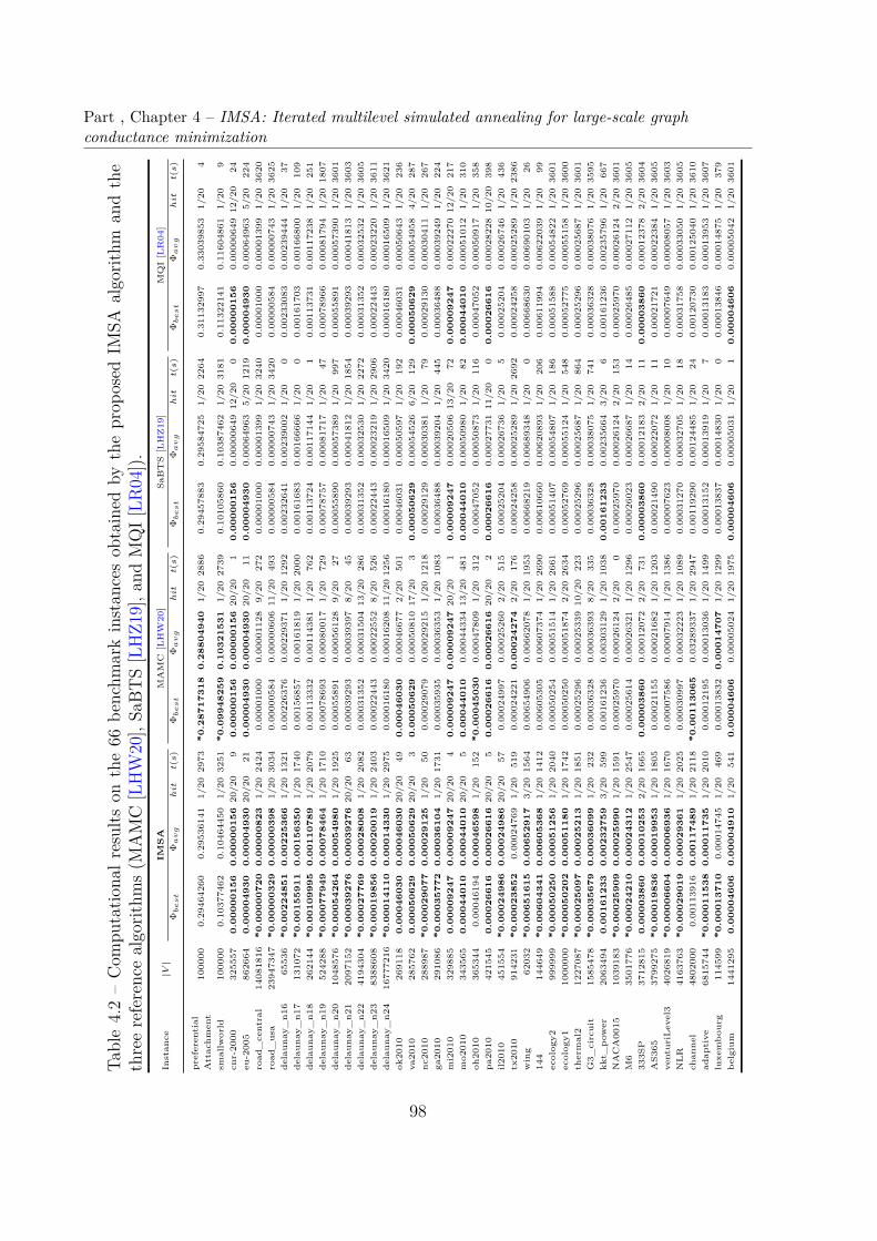
Part , Chapter 4 – IMSA: Iterated multilevel simulated annealing for large-scale graphconductance minimization
Table4.2–Com
putatio
nalr
esults
onthe66
benchm
arkinstan
cesob
tained
bytheprop
osed
IMSA
algorit
hman
dthe
threereferencealgorit
hms(M
AMC
[LHW
20],Sa
BTS[LHZ1
9],a
ndMQI[LR
04]).
IMS
AMAMC
[LHW20]
SaBTS[LHZ19]
MQI[LR04]
Instan
ce|V
|Φ
be
st
Φa
vg
hit
t(s)
Φb
es
tΦ
av
ghit
t(s)
Φb
es
tΦ
av
ghit
t(s)
Φb
es
tΦ
av
ghit
t(s)
preferential
Attachm
ent
100000
0.29464260
0.29536141
1/20
2973
*0
.28
71
73
18
0.2
88
04
94
01/20
2886
0.29457883
0.29584725
1/20
2264
0.31132997
0.33039853
1/20
4
smallworld
100000
0.10377462
0.10464450
1/20
3251
*0
.09
94
82
59
0.1
03
21
53
11/20
2739
0.10105860
0.10387462
1/20
3181
0.11322141
0.11604861
1/20
9cnr-2000
325557
0.0
00
00
15
60
.00
00
01
56
20/20
90
.00
00
01
56
0.0
00
00
15
620/20
10
.00
00
01
56
0.00000649
12/20
00
.00
00
01
56
0.00000649
12/20
24eu-2005
862664
0.0
00
04
93
00
.00
00
49
30
20/20
210
.00
00
49
30
0.0
00
04
93
020/20
110
.00
00
49
30
0.00064963
5/20
1219
0.0
00
04
93
00.00064963
5/20
224
road
_central
14081816
*0
.00
00
07
20
0.0
00
00
82
31/20
2424
0.00001000
0.00001128
9/20
272
0.00001000
0.00001399
1/20
3240
0.00001000
0.00001399
1/20
3620
road
_usa
23947347
*0
.00
00
03
29
0.0
00
00
39
81/20
3034
0.00000584
0.00000606
11/20
493
0.00000584
0.000007
431/20
3420
0.00000584
0.00000743
1/20
3625
delaun
ay_n1
665536
*0
.00
22
48
51
0.0
02
25
36
61/20
1321
0.00226376
0.00229371
1/20
1292
0.00232641
0.002390
021/20
00.00233083
0.00239444
1/20
37delaun
ay_n1
7131072
*0
.00
15
59
11
0.0
01
56
35
01/20
1740
0.00156857
0.00161819
1/20
2000
0.00161683
0.001666
661/20
00.00161703
0.00166800
1/20
109
delaun
ay_n1
8262144
*0
.00
10
99
95
0.0
01
10
78
91/20
2079
0.00113332
0.00114381
1/20
762
0.00113724
0.00117144
1/20
10.00113731
0.00117238
1/20
251
delaun
ay_n1
9524288
*0
.00
07
79
49
0.0
00
78
46
41/20
1710
0.00078693
0.00080017
1/20
729
0.00078757
0.00081717
1/20
470.00078966
0.00081794
1/20
1807
delaun
ay_n2
01048576
*0
.00
05
42
64
0.0
00
54
98
01/20
1925
0.00055891
0.00056128
9/20
270.00055890
0.00057389
1/20
997
0.00055891
0.00057390
1/20
3601
delaun
ay_n2
12097152
*0
.00
03
92
76
0.0
00
39
27
620/20
630.00039293
0.00039397
8/20
450.00039293
0.00041812
1/20
1854
0.00039293
0.00041813
1/20
3603
delaun
ay_n2
24194304
*0
.00
02
77
69
0.0
00
28
00
81/20
2082
0.00031352
0.00031504
13/20
286
0.00031352
0.000325
301/20
2272
0.00031352
0.00032532
1/20
3605
delaun
ay_n2
38388608
*0
.00
01
98
56
0.0
00
20
01
91/20
2403
0.00022443
0.00022552
8/20
526
0.00022443
0.00023219
1/20
2906
0.00022443
0.00023220
1/20
3611
delaun
ay_n2
416777216
*0
.00
01
41
10
0.0
00
14
33
01/20
2975
0.00016180
0.00016208
11/201256
0.00016180
0.00016509
1/20
3420
0.00016180
0.00016509
1/20
3621
ok2010
269118
0.0
00
46
03
00
.00
04
60
30
20/20
490
.00
04
60
30
0.00046677
2/20
501
0.00046031
0.00050597
1/20
192
0.00046031
0.00050643
1/20
236
va2010
285762
0.0
00
50
62
90
.00
05
06
29
20/20
30
.00
05
06
29
0.00050810
17/20
30
.00
05
06
29
0.00054526
6/20
129
0.0
00
50
62
90.00054958
4/20
287
nc2010
288987
*0
.00
02
90
77
0.0
00
29
12
51/20
500.00029079
0.00029215
1/20
1218
0.00029129
0.00030381
1/20
790.00029130
0.00030411
1/20
267
ga2010
291086
*0
.00
03
57
72
0.0
00
36
10
41/20
1731
0.00035935
0.00036353
1/20
1083
0.00036488
0.000392
041/20
445
0.00036488
0.00039249
1/20
224
mi2010
329885
0.0
00
09
24
70
.00
00
92
47
20/20
40
.00
00
92
47
0.0
00
09
24
720/20
10
.00
00
92
47
0.00020506
13/20
720
.00
00
92
47
0.00022270
12/20
217
mo2010
343565
0.0
00
44
01
00
.00
04
40
10
20/20
50
.00
04
40
10
0.00044334
13/20
481
0.0
00
44
01
00.00050980
1/20
820
.00
04
40
10
0.00051012
1/20
310
oh2010
365344
0.00
046194
0.0
00
46
59
81/20
152
*0
.00
04
50
30
0.00047809
1/20
312
0.00047052
0.00050873
1/20
116
0.00047052
0.00050917
1/20
358
pa2010
421545
0.0
00
26
61
60
.00
02
66
16
20/20
50
.00
02
66
16
0.0
00
26
61
620/20
20
.00
02
66
16
0.00027731
11/20
00
.00
02
66
16
0.00028228
10/20
398
il2010
451554
*0
.00
02
49
86
0.0
00
24
98
620/20
570.00024997
0.00025260
2/20
515
0.00025204
0.00026736
1/20
50.00025204
0.00026746
1/20
436
tx2010
914231
*0
.00
02
38
52
0.00024769
1/20
519
0.00024221
0.0
00
24
27
42/20
176
0.00024258
0.00025289
1/20
2692
0.00024258
0.00025289
1/20
2386
wing
62032
*0
.00
65
16
15
0.0
06
52
91
73/20
1564
0.00654906
0.00662078
1/20
1953
0.00668219
0.006893
481/20
00.00668630
0.00690103
1/20
26144
144649
*0
.00
60
43
41
0.0
06
05
36
81/20
1412
0.00605305
0.00607374
1/20
2690
0.00610660
0.006208
931/20
206
0.00611994
0.00622039
1/20
99ecology2
999999
*0
.00
05
02
50
0.0
00
51
25
61/20
2040
0.00050254
0.00051514
1/20
2661
0.00051407
0.000548
071/20
186
0.00051588
0.00054822
1/20
3601
ecology1
1000000
*0
.00
05
02
02
0.0
00
51
18
01/20
1742
0.00050250
0.00051874
2/20
2634
0.00052769
0.000551
241/20
548
0.00052775
0.00055158
1/20
3600
thermal2
1227087
*0
.00
02
50
97
0.0
00
25
21
31/20
1851
0.00025296
0.00025339
10/20
223
0.00025296
0.000256
871/20
864
0.00025296
0.00025687
1/20
3601
G3_
circuit
1585478
*0
.00
03
56
79
0.0
00
36
09
91/20
232
0.00036328
0.00036393
8/20
335
0.00036328
0.00038075
1/20
741
0.00036328
0.00038076
1/20
3595
kkt_
pow
er2063494
0.0
01
61
23
30
.00
23
27
59
3/20
599
0.00161236
0.00303129
1/20
1038
0.0
01
61
23
30.00235664
3/20
60.00161236
0.00235796
1/20
667
NACA0015
1039183
*0
.00
02
59
09
0.0
00
25
99
01/20
1591
0.00025970
0.00026124
2/20
00.00025970
0.00026124
2/20
153
0.00025970
0.00026124
2/20
3601
M6
3501776
*0
.00
02
42
10
0.0
00
24
31
21/20
2547
0.00025614
0.00026321
1/20
1296
0.00026023
0.000266
871/20
140.00026485
0.00027112
1/20
3605
333S
P3712815
0.0
00
03
86
00
.00
01
02
53
2/20
1665
0.0
00
03
86
00.00012072
2/20
731
0.0
00
03
86
00.00012183
2/20
110
.00
00
38
60
0.00012378
2/20
3604
AS3
653799275
*0
.00
01
98
36
0.0
00
19
95
31/20
1805
0.00021155
0.00021682
1/20
1203
0.00021490
0.000220
721/20
110.00021721
0.00022384
1/20
3605
venturiLevel3
4026819
*0
.00
00
66
04
0.0
00
06
93
61/20
1670
0.00007586
0.00007914
1/20
1386
0.00007623
0.000080
081/20
100.00007649
0.00008057
1/20
3603
NLR
4163763
*0
.00
02
90
19
0.0
00
29
36
11/20
2025
0.00030997
0.00032223
1/20
1089
0.00031270
0.000327
051/20
180.00031758
0.00033050
1/20
3605
chan
nel
4802000
0.00113916
0.0
01
17
48
91/20
2118
*0
.00
11
30
65
0.03289337
1/20
2947
0.00119290
0.00124485
1/20
240.00120730
0.00125040
1/20
3610
adap
tive
6815744
*0
.00
01
15
38
0.0
00
11
73
51/20
2010
0.00012195
0.00013036
1/20
1499
0.00013152
0.000139
191/20
70.00013183
0.00013953
1/20
3607
luxembou
rg114599
*0
.00
01
37
10
0.00014745
1/20
469
0.00013832
0.0
00
14
70
71/20
1299
0.00013837
0.00014830
1/20
00.00013846
0.00014875
1/20
379
belgium
1441295
0.0
00
04
60
60
.00
00
49
10
1/20
541
0.0
00
04
60
60.00005024
1/20
1975
0.0
00
04
60
60.00005031
1/20
10
.00
00
46
06
0.00005042
1/20
3601
98
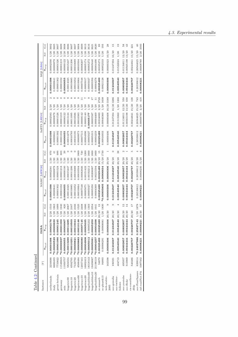
4.3. Experimental resultsTa
ble4.2:
Con
tinued
IMS
AMAMC
[LHW20]
SaBTS[LHZ19]
MQI[LR04]
Instan
ce|V
|Φ
be
st
Φa
vg
hit
t(s)
Φb
es
tΦ
av
ghit
t(s)
Φb
es
tΦ
av
ghit
t(s)
Φb
es
tΦ
av
ghit
t(s)
netherland
s2216688
0.0
00
01
09
80
.00
00
21
76
2/20
1510
0.0
00
01
09
80.00002581
1/20
970
0.0
00
01
09
80.00002583
2/20
20
.00
00
10
98
0.00002590
1/20
3602
italy
6686493
*0
.00
00
05
29
0.0
00
00
63
01/20
1863
0.00000641
0.00000878
1/20
410.00000641
0.00000878
1/20
00.00000641
0.00000878
1/20
3605
great-britain
7733822
*0
.00
00
10
90
0.0
00
01
24
51/20
1689
0.00001302
0.00001524
1/20
689
0.00001302
0.00001526
1/20
00.00001302
0.00001526
1/20
3607
germ
any
11548845
*0
.00
00
09
37
0.0
00
01
00
01/20
1940
0.00001032
0.00001218
1/20
603
0.00001032
0.00001219
1/20
00.00001032
0.00001219
1/20
3609
asia
11950757
0.0
00
00
05
50
.00
00
00
67
7/20
820
0.0
00
00
05
50.00000100
7/20
390
.00
00
00
55
0.00000122
7/20
00
.00
00
00
55
0.00000122
2/20
3608
hugetric00
5824554
*0
.00
01
32
90
0.0
00
14
28
51/20
2067
0.00014325
0.00015247
1/20
00.00014278
0.00015124
1/20
90.00014325
0.00015247
1/20
3606
hugetric10
6592765
*0
.00
01
02
51
0.0
00
10
50
31/20
2167
0.00010885
0.00011206
1/20
00.00010783
0.00011095
1/20
80.00010885
0.00011206
1/20
3607
hugetric20
7122792
*0
.00
00
98
21
0.0
00
10
04
41/20
2166
0.00010252
0.00010689
1/20
00.00010195
0.00010586
1/20
80.00010252
0.00010689
1/20
3607
hugetrace00
4588484
*0
.00
00
98
83
0.0
00
10
14
81/20
1525
0.00010064
0.00010504
1/20
1869
0.00009973
0.00010383
1/20
90.00010064
0.00010504
1/20
3604
hugetrace10
12057441
*0
.00
00
60
80
0.0
00
07
14
51/20
2408
0.00007548
0.00082926
1/20
720
0.00007515
0.00008142
1/20
110.00007548
0.00008207
1/20
3609
hugetrace20
16002413
*0
.00
00
49
08
0.0
00
05
03
51/20
1686
0.00005071
0.00151422
1/20
1260
0.00004996
0.00005140
1/20
70.00005017
0.00005174
1/20
3613
hugebu
bbles00
18318143
*0
.00
00
50
12
0.00005232
2/20
1303
0.00005027
0.00192212
1/20
1800
0.00005027
0.0
00
05
17
71/20
90.00005027
0.00005272
1/20
3616
hugebu
bbles10
19458087
*0
.00
00
50
81
0.0
00
05
25
91/20
2354
0.00005350
0.00206087
1/20
1800
0.00005315
0.00005587
1/20
170.00005356
0.000056
401/20
3621
hugebu
bbles20
21198119
*0
.00
00
42
57
0.0
00
04
39
81/20
1641
0.00004369
0.00215594
1/20
1800
0.00004259
0.00004469
1/20
110.00004278
0.000044
901/20
3620
sc-nasasrb
54870
0.0
03
25
48
90
.00
32
54
89
20/20
120
.00
32
54
89
0.0
03
25
48
920/20
150
.00
32
54
89
0.00334089
2/20
2728
0.0
03
25
48
90.00335273
2/20
89sc-pku
stk1
394893
0.00906291
0.00908081
1/20
1830
*0
.00
90
58
05
0.0
09
06
63
415/201730
0.00916933
0.00946360
1/20
1638
0.00921128
0.00952533
1/20
193
web-arabic-
2005
163598
0.0
00
00
30
60
.00
00
03
06
20/20
90
.00
00
03
06
0.0
00
00
30
620/20
10.00000406
0.00000408
16/203189
0.0
00
00
30
60.00000323
10/20
28
soc-gowalla
196591
0.0
12
34
56
70
.01
23
45
67
20/20
90
.01
23
45
67
0.0
12
34
56
720/20
00
.01
23
45
67
0.01247394
16/203286
0.0
12
34
56
70.01247394
16/20
15soc-tw
itter-
follow
s404719
0.0
05
40
54
00
.00
54
05
40
20/20
40
.00
54
05
40
0.0
05
40
54
020/20
380
.00
54
05
40
0.01515060
1/20
1260
0.0
05
40
54
00.01522024
1/20
19
soc-yo
utub
e495957
0.0
08
92
85
70
.00
89
28
57
20/20
120
.00
89
28
57
0.0
08
92
85
720/20
20
.00
89
28
57
0.01134011
12/20
550
0.0
08
92
85
70.01134011
12/20
58soc-flickr
513969
0.0
04
44
44
40
.00
44
44
44
20/20
140
.00
44
44
44
0.0
04
44
44
420/20
10
.00
44
44
44
0.00565198
13/20
658
0.0
04
44
44
40.00565198
13/20
43ca-coautho
rs-
dblp
540486
0.0
02
26
75
70
.00
22
67
57
20/20
170
.00
22
67
57
0.0
02
26
75
720/20
50
.00
22
67
57
0.00244841
15/20
108
0.0
02
26
75
70.00244841
15/20
221
soc-Fou
rSqu
are
639014
*0
.24
62
79
88
0.2
58
27
14
21/20
1878
0.26530612
0.26530612
20/20
40.26530612
0.26564625
15/20
743
0.26530612
0.26564625
15/20
40inf-road
Net-PA
1087562
0.0
00
08
22
10
.00
00
82
21
20/20
570
.00
00
82
21
0.00008230
15/20
40
.00
00
82
21
0.00008789
2/20
418
0.0
00
08
22
10.00008789
2/20
3593
99
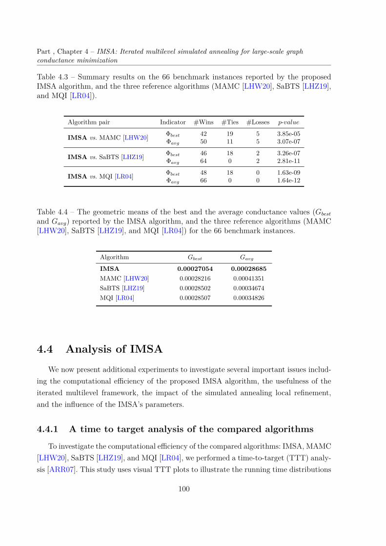
Part , Chapter 4 – IMSA: Iterated multilevel simulated annealing for large-scale graphconductance minimization
Table 4.3 – Summary results on the 66 benchmark instances reported by the proposedIMSA algorithm, and the three reference algorithms (MAMC [LHW20], SaBTS [LHZ19],and MQI [LR04]).
Algorithm pair Indicator #Wins #Ties #Losses p-value
IMSA vs. MAMC [LHW20] Φbest 42 19 5 3.85e-05Φavg 50 11 5 3.07e-07
IMSA vs. SaBTS [LHZ19] Φbest 46 18 2 3.26e-07Φavg 64 0 2 2.81e-11
IMSA vs. MQI [LR04] Φbest 48 18 0 1.63e-09Φavg 66 0 0 1.64e-12
Table 4.4 – The geometric means of the best and the average conductance values (Gbest
and Gavg) reported by the IMSA algorithm, and the three reference algorithms (MAMC[LHW20], SaBTS [LHZ19], and MQI [LR04]) for the 66 benchmark instances.
Algorithm Gbest Gavg
IMSA 0.00027054 0.00028685MAMC [LHW20] 0.00028216 0.00041351SaBTS [LHZ19] 0.00028502 0.00034674MQI [LR04] 0.00028507 0.00034826
4.4 Analysis of IMSA
We now present additional experiments to investigate several important issues includ-ing the computational efficiency of the proposed IMSA algorithm, the usefulness of theiterated multilevel framework, the impact of the simulated annealing local refinement,and the influence of the IMSA’s parameters.
4.4.1 A time to target analysis of the compared algorithms
To investigate the computational efficiency of the compared algorithms: IMSA, MAMC[LHW20], SaBTS [LHZ19], and MQI [LR04], we performed a time-to-target (TTT) analy-sis [ARR07]. This study uses visual TTT plots to illustrate the running time distributions
100
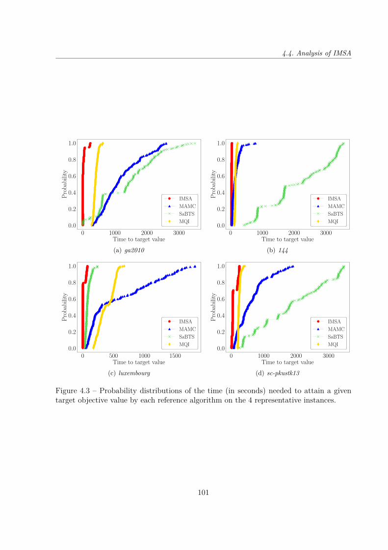
4.4. Analysis of IMSA
0 1000 2000 3000Time to target value
0.0
0.2
0.4
0.6
0.8
1.0
Pro
bab
ility
IMSA
MAMC
SaBTS
MQI
(a) ga2010
0 1000 2000 3000Time to target value
0.0
0.2
0.4
0.6
0.8
1.0
Pro
bab
ility
IMSA
MAMC
SaBTS
MQI
(b) 144
0 500 1000 1500Time to target value
0.0
0.2
0.4
0.6
0.8
1.0
Pro
bab
ility
IMSA
MAMC
SaBTS
MQI
(c) luxembourg
0 1000 2000 3000Time to target value
0.0
0.2
0.4
0.6
0.8
1.0
Pro
bab
ility
IMSA
MAMC
SaBTS
MQI
(d) sc-pkustk13
Figure 4.3 – Probability distributions of the time (in seconds) needed to attain a giventarget objective value by each reference algorithm on the 4 representative instances.
101

Part , Chapter 4 – IMSA: Iterated multilevel simulated annealing for large-scale graphconductance minimization
of the compared algorithms. Specifically, the Y-axis of the TTT plots displays the prob-ability that an algorithm will find a solution that is at least as good as a given targetvalue within a given run time, shown on the X-axis. The TTT plots are produced asfollows. Each compared algorithm is independently run Ex times on each instance. Foreach of the Ex runs, the run time to reach a given target objective value is recorded. Foreach instance, the run times are then sorted in an ascending order. We associate the i-thsorted run time ti with a probability pi = (i − 0.5)/Ex, and plot the points (ti, pi), fori = 1, . . . , Ex. Our TTT experiment was based on 4 representative instances: (ga2010,144, luxembourg, sc-pkustk13 ) with 200 independent runs per algorithm and per instance(i.e., Ex = 200). To make sure that all the compared algorithms are able to reach thetarget objective value in each run, we set the target value to be 1% larger than the bestobjective value found by MQI. The results of this experiment are shown in Fig. 4.3. Theseplots clearly indicate that the proposed IMSA algorithm is always faster in attaining thegiven target value than the reference algorithms. For example, the probability that IMSAreaches the target objective value for instances ga2010 and sc-pkustk13 in the first 100seconds is around 90%, while MAMC, SaBTS, and MQI require at least 2000 seconds,3500 seconds, and 500 seconds respectively to attain the same result. This experimentdemonstrates that the proposed IMSA algorithm is much more time efficient than thereference algorithms.
4.4.2 Usefulness of the iterated multilevel framework
In this section, we assess the usefulness of the iterated multilevel framework. For thispurpose, we created an IMSA variant called (SA+TS)restart where the multilevel com-ponent was removed while keeping only the refinement procedure (SA and tabu search).To ensure a fair comparison, we performed (SA+TS)restart in a multi-start way, untilthe cutoff time tmax (60 minutes) was reached. This experiment was conducted on 20instances of a reasonable size and difficulty: (preferentialAttachment, smallworld, delau-nay_n16, delaunay_n17, delaunay_n18, delaunay_n19, ga2010, oh2010, tx2010, wing,144, ecology2, ecology1, thermal2, kkt_power, NACA0015, M6, AS365, luxembourg, bel-gium). Each algorithm was independently run 20 times per instance with a cutoff timeof 60 minutes per run. Fig. 4.4 shows the best/average conductance gap between the twoalgorithms on these instances. The X-axis indicates the instance label (numbered from 1to 20), while the Y-axis shows the best/average conductance gap in percentage, calculatedas (ΦA − ΦIMSA)/ΦIMSA × 100%, where ΦA and ΦIMSA are the best/average conductance
102

4.4. Analysis of IMSA
1 2 3 4 5 6 7 8 9 10 11 12 13 14 15 16 17 18 19 20
Instance label
0
1
2
3
4
Bes
tco
nd
uct
ance
gap
(%)
(SA+TS)restart
IMSA
(a) Best results
1 2 3 4 5 6 7 8 9 10 11 12 13 14 15 16 17 18 19 20
Instance label
0
2
4
6
8
Ave
rage
con
du
ctan
cega
p(%
)
(SA+TS)restart
IMSA
(b) Average results
Figure 4.4 – Comparisons of the proposed IMSA algorithm with a multi-start simulatedannealing plus tabu search (denoted by (SA+TS)restart) on 20 representative instances.
values of (SA+TS)restart and IMSA, respectively.As observed in Fig. 4.4, IMSA clearly dominates (SA+TS)restart in terms of the best
and the average conductance values for the 20 instances. This experiment confirms theusefulness of the iterated multilevel framework, which positively contributes to the highperformance of the proposed IMSA algorithm.
4.4.3 Benefit of the SA-based local refinement
To evaluate the benefit of the SA local refinement procedure to the performance of theproposed IMSA algorithm, we created a variant of IMSA (denoted by IMSAdescent) wherewe replaced the SA procedure by a pure descent procedure using the best-improvementstrategy. This experiment relies on the same 20 representative instances used in Section4.4.2 and reports the same information. Fig. 4.5 plots the best/average conductance gapof the two algorithms on these instances. The X-axis indicates the instance label, whilethe Y-axis shows the best/average conductance gap in percentage.
From Fig. 4.5, we observe that IMSAdescent reports worse results in terms of both thebest and the average conductance values for all the instances. This indicates that the SAprocedure is the key element that ensures the high performance of IMSA and disabling itgreatly deteriorates the performance.
103

Part , Chapter 4 – IMSA: Iterated multilevel simulated annealing for large-scale graphconductance minimization
1 2 3 4 5 6 7 8 9 10 11 12 13 14 15 16 17 18 19 20
Instance label
0
2
4
6
8
Bes
tco
nd
uct
ance
gap
(%)
IMSAdescent
IMSA
(a) Best results
1 2 3 4 5 6 7 8 9 10 11 12 13 14 15 16 17 18 19 20
Instance label
0
2
4
6
8
10
12
Ave
rage
con
du
ctan
cega
p(%
)
IMSAdescent
IMSA
(b) Average results
Figure 4.5 – Comparisons of the proposed IMSA algorithm with an IMSA variant wherethe SA-based local refinement is replaced by a descent search (denoted by IMSAdescent)on the 20 representative instances.
4.4.4 Analysis of the parameters
The proposed IMSA algorithm requires six parameters: ct, saIter, θ, ar, D, and α. Weuse ct to denote the coarsening threshold in the solution-guided coarsening phase. saIter,θ, and ar are the three parameters related to the SA local refinement, where saIter isthe maximum number of iterations per temperature, θ is the cooling ratio, and ar is thefrozen state parameter. D and α are the depth of tabu search and the tabu tenure man-agement factor, respectively. To study the effect of these parameters on the performanceof IMSA and to determine the most suitable setting for these parameters, we carried outan experiment as follows. For each parameter, we tested a range of possible values, whilefixing the other parameters to their default values from Table 4.1. Specifically, we testedthe following values: ct ∈ [20000, 30000, 40000, 50000, 60000], saIter ∈ [50000, 100000,150000, 200000, 250000], θ ∈ [0.90, 0.92, 0.94, 0.96, 0.98], ar ∈ [1%, 3%, 5%, 7%, 9%],D ∈ [5000, 10000, 15000, 20000, 25000], and α ∈ [40, 60, 80, 100, 120]. This experimentwas conducted on 9 representative instances from the set of instances used in Sections4.4.2 and 4.4.3, and based on 20 independent runs per parameter value with a cutoff timeof 60 minutes per run. Fig. 4.6 shows the average values of Φbest and Φavg obtained forthe 9 instances, where the X-axis indicates the values of each parameter and the Y-axisshows the best/average conductance values over the 9 representative instance: (prefer-
104
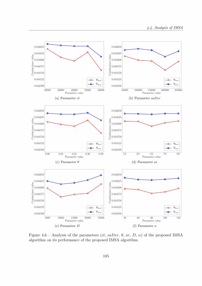
4.4. Analysis of IMSA
20000 30000 40000 50000 60000Parameter value
0.044500
0.044525
0.044550
0.044575
0.044600
0.044625
0.044650
Con
du
ctan
ceva
lue
Φbest
Φavg
(a) Parameter ct
50000 100000 150000 200000 250000Parameter value
0.044500
0.044525
0.044550
0.044575
0.044600
0.044625
0.044650
Con
du
ctan
ceva
lue
Φbest
Φavg
(b) Parameter saIter
0.90 0.92 0.94 0.96 0.98Parameter value
0.044500
0.044525
0.044550
0.044575
0.044600
0.044625
0.044650
Con
du
ctan
ceva
lue
Φbest
Φavg
(c) Parameter θ
1% 3% 5% 7% 9%Parameter value
0.044500
0.044525
0.044550
0.044575
0.044600
0.044625
0.044650C
ond
uct
ance
valu
e
Φbest
Φavg
(d) Parameter ar
5000 10000 15000 20000 25000Parameter value
0.044500
0.044525
0.044550
0.044575
0.044600
0.044625
0.044650
Con
du
ctan
ceva
lue
Φbest
Φavg
(e) Parameter D
40 60 80 100 120Parameter value
0.044500
0.044525
0.044550
0.044575
0.044600
0.044625
0.044650
Con
du
ctan
ceva
lue
Φbest
Φavg
(f) Parameter α
Figure 4.6 – Analysis of the parameters (ct, saIter, θ, ar, D, α) of the proposed IMSAalgorithm on its performance of the proposed IMSA algorithm.
105

Part , Chapter 4 – IMSA: Iterated multilevel simulated annealing for large-scale graphconductance minimization
entialAttachment, smallworld, delaunay_n18, delaunay_n19, ga2010, oh2010, wing, 144,thermal2 ).
Fig. 4.6 shows the impact of each parameter on the performance of IMSA. Specifically,for the parameter ct, ct = 60000 yields the best results for both Φbest and Φavg. We thusset the default value of ct to 60000 in this study. For saIter, the value of 200000 is thebest choice while a larger or a smaller value weakens the performance of IMSA. For theparameter θ, IMSA obtains the best performance with the value of 0.98 while smallervalues decrease its performance. Furthermore, ar = 5% appears to be the best choice forIMSA. For the parameters D and α, we choose the value 10000 and 80 respectively astheir default values according to Fig. 4.6. The default values of all the parameters aresummarized in Table 4.1.
4.5 Conclusion
The iterated multilevel simulated annealing algorithm (IMSA) presented in this workis the first multilevel algorithm dedicated to the challenging NP-hard minimum conduc-tance graph partitioning problem (MC-GPP). Based on the general (iterated) multileveloptimization framework, IMSA integrates an original solution-guided coarsening methodto construct a hierarchy of reduced graphs and a powerful simulated annealing local re-finement procedure that makes full use of a constrained neighborhood to rapidly andeffectively improve the quality of sampled solutions.
We assessed the performance of IMSA on two sets of 66 very large benchmark instancesfrom the literature, including 56 graphs from the 10th DIMACS Implementation ChallengeBenchmark and 10 graphs from the Network Data Repository online, with up to 23 millionvertices. Computational results demonstrated high competitiveness of the proposed IMSAalgorithm compared to three state-of-the-art methods. Particularly, IMSA improved onthe current best-known result for 41 out of the 66 large-scale benchmark instances, whilereaching the same solution quality as the existing state-of-art algorithms on 22 remaininggraphs. Only for 5 instances, IMSA was unable to reach the best-know solution fromthe literature. We presented additional experiments to get insights into the design of theproposed IMSA algorithm including the usefulness of the iterated multilevel framework,the impact of the simulated annealing local refinement procedure, and its parameters.Given the numerous important applications of MC-GPP, the proposed approach couldconstitute a valuable strategy for improved performance on these real world problems. The
106

4.5. Conclusion
availability of the source code of our algorithm will further facilitate such applications.
107


GENERAL CONCLUSION
Conclusions
This thesis focuses on devising effective heuristics and metaheuristics algorithms forsolving the well-known NP-hard minimum conductance graph partitioning problem (MC-GPP). Due to the theoretical intractability and the widespread real world applications ofMC-GPP, we studied several solution methods to find high quality sub-optimal solutionsfor large scale benchmark instances in acceptable computing time. The resulting algo-rithms are implemented and evaluated on a number of well-known benchmark instancesand shown to be highly competitive in comparison with the best performing algorithmsin the literature.
In Chapter 2, we presented a stagnation-aware breakout tabu search algorithm (SaBTS)for MC-GPP. SaBTS integrates two noteworthy features: a constrained neighborhood tabusearch procedure to discover high quality solutions and a self-adaptive and multi-strategyperturbation procedure to overcome hard-to-escape local optimum traps. We assessed theeffectiveness of the proposed SaBTS algorithm with state-of-the-art algorithms on fivedatasets of 110 benchmark instances with up to around 500 000 vertices in the literature,including 98 graphs from the 10th DIMACS Implementation Challenge Benchmark and 12anonymized social networks. The computational results indicated that SaBTS dominatesa recent dedicated algorithm StS-AMA [Cha17; CHW18]. Moreover, when SaBTS is runas a post-processing method, it consistently improves on the solutions provided by thepopular graph partitioning tool Metis [KK98b] and the state-of-the-art max-flow-basedmethod MQI [LR04]. Additional experiments investigated the key components of SaBTS,including the effect of the parameters, the impact of the constrained neighborhood ontabu search, as well as the impact of the perturbation strategy, which contribute to theperformance of the proposed SaBTS algorithm.
In Chapter 3, we explored an effective hybrid evolutionary algorithm (MAMC) forMC-GPP. Based on the population memetic search framework, MAMC integrates someimportant features. 1) To ensure an effective and efficient intensification of its local opti-mization component on large graphs, MAMC adopts an original progressive neighborhood
109

whose size is dynamically adjusted according to the search state. 2) To maintain a healthypopulation of high diversity and good quality, MAMC uses a proven distance-and-qualitypool updating strategy for its population management. 3) To further diversify the search,a conventional crossover is applied to generate offspring solutions. We tested the proposedMAMC algorithm on 60 very large real world benchmark instances, including 50 graphsfrom the 10th DIMACS Implementation Challenge Benchmark and 10 graphs from theNetwork Data Repository online, with up to 23 million vertices. The results demonstratedMAMC competes very favorably with the current best-performing algorithms, and led tothe main conclusions that 1) MAMC dominates the reference algorithms for the testedinstances, and 2) it is able to further improve the solutions obtained by the popularmax-flow-based method MQI [LR04]. As an additional assessment, we showed an applica-tion of using the proposed MAMC algorithm to detect community structures in complexnetworks. Finally, we investigated the essential components of the proposed MAMC al-gorithm, leading to the findings that 1) the progressive neighborhood used by the localoptimization procedure plays an important role of ensuring a fast convergence of the algo-rithm, and 2) the quality-and-diversity pool initialization and distance-and-quality poolmanagement help the algorithm to maintain a healthy population, which contributes toits high performance.
In Chapter 4, we designed the first multilevel algorithm called an iterated multilevelsimulated annealing algorithm (IMSA) dedicated to the challenging NP-hard MC-GPP.Based on the general (iterated) multilevel optimization framework, IMSA features anoriginal solution-guided coarsening method to construct a hierarchy of reduced graphsand a powerful simulated annealing local refinement procedure that makes full use of aconstrained neighborhood to effectively sample the search space of the problem. Exten-sive computational assessments on two sets of 66 very large benchmark instances in theliterature (including 56 graphs from the 10th DIMACS Implementation Challenge Bench-mark and 10 graphs from the Network Data Repository online, with up to 23 millionvertices) have demonstrated the high competitiveness of the proposed IMSA algorithm.Particularly, IMSA reported strictly best solutions for 41 very large instances out of the66 benchmark graphs, while reaching equal best solutions reported by the reference al-gorithms for 20 other graphs. Only for 5 instances, IMSA performed slightly worse. Weperformed additional experiments to get insights into the design of the proposed IMSAalgorithm including the usefulness of the iterated multilevel framework, the impact of thesimulated annealing local refinement procedure, and its parameters.
110
Perspectives
From the work presented in this thesis, several interesting perspectives can be identifiedfor future research.
First, as the results of Metis suggest, optimizing the number of cut edges helps tofind partitions of relatively low conductance. Therefore, one interesting study would beto investigate the use of cut-edge criterion as an approximate evaluation function of con-ductance in search algorithms. Indeed, one can take advantage of the well-known efficientdata structures and fast incremental update techniques available for the cut-edge criterion,helping to significantly reduce the computational cost of search algorithms for MC-GPP.
Second, the idea of the progressive neighborhood strategy proposed in Chapter 3 isof general interest, it would be interesting to test the idea in other settings, in particularrelated to large graph optimization. The study of Chapter 4 demonstrated the benefit ofthe iterated multilevel framework and its simulated annealing local refinement procedurefor large scale graph partitioning with the conductance criterion. The underlying ideas ofthis work could be useful for designing effective algorithms for other graph partitioningand clustering problems, especially for dealing with large graphs.
Third, until now, there are still very few effective exact algorithms for MC-GPP inthe literature. It is thus worth investigating general approaches such as integer linearprogramming and dedicated branch and bound algorithms.
111

APPENDIX
Chapter 2
This appendix provides the detailed computational results presented in Section 2.3.3.Table A.1 shows the detailed results of algorithms Metis [KK98b], Metis+MQI [LR04],Metis+SaBTS, and (Metis+MQI)+SaBTS for the five datasets including 110 graphs. Asexplained in Section 2.3.3, these results are based on 20 independent runs of each algorithmto solve each instance with a cutoff limit of 60 minutes per run and per instance. Φbest ofan algorithm for an instance indicates the lowest conductance achieved for the instanceamong the conductance values of the 20 runs, while Φavg is the average of the 20 Φbest
values. The best of the Φbest values for each instance is highlighted in boldface, while thebest of the Φavg values for each instance is indicated in italic. t(s) is the average CPUtime in seconds of 20 runs to attain the 20 best results, and a time less than one secondis indicated as 0. These best values can be used to evaluate other MC-GPP algorithms.Table A.2 shows the statistical results (p-values) from the Wilcoxon signed-rank test witha confidence level of 99% applied to different pairwise comparisons for all datasets. Thetests are performed on the Φbest and Φavg values.
To complete the computational comparison presented in Section 2.3.3, we show inTable A.3 an additional comparison of the studied algorithms using the geometric meanmetric [FW86; HB97] calculated with the best and average conductance values of eachcompared algorithm (Gbest and Gavg) on five datasets. The best values of Gbest are high-lighted in boldface while the best values of Gavg are indicated in italic. A small valueindicates a better performance.
113
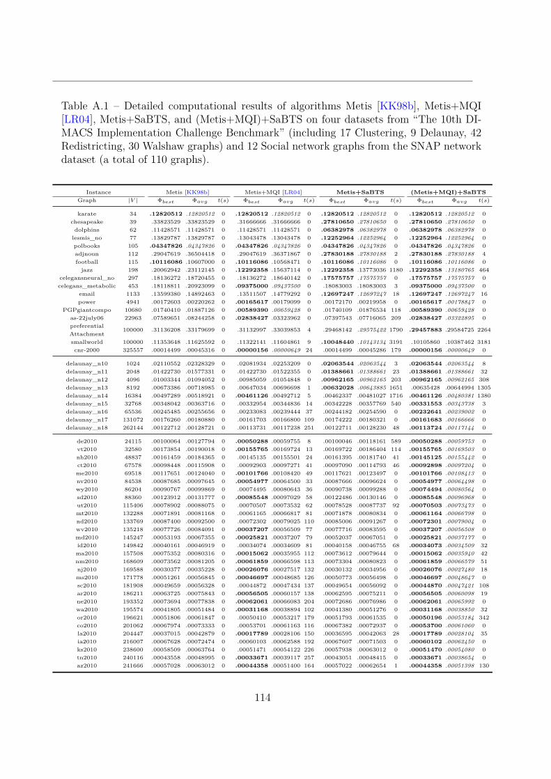
Table A.1 – Detailed computational results of algorithms Metis [KK98b], Metis+MQI[LR04], Metis+SaBTS, and (Metis+MQI)+SaBTS on four datasets from “The 10th DI-MACS Implementation Challenge Benchmark” (including 17 Clustering, 9 Delaunay, 42Redistricting, 30 Walshaw graphs) and 12 Social network graphs from the SNAP networkdataset (a total of 110 graphs).
Instance Metis [KK98b] Metis+MQI [LR04] Metis+SaBTS (Metis+MQI)+SaBTSGraph |V | Φbest Φavg t(s) Φbest Φavg t(s) Φbest Φavg t(s) Φbest Φavg t(s)
karate 34 .12820512 .12820512 0 .12820512 .12820512 0 .12820512 .12820512 0 .12820512 .12820512 0chesapeake 39 .33823529 .33823529 0 .31666666 .31666666 0 .27810650 .27810650 0 .27810650 .27810650 0dolphins 62 .11428571 .11428571 0 .11428571 .11428571 0 .06382978 .06382978 0 .06382978 .06382978 0lesmis_no 77 .13829787 .13829787 0 .13043478 .13043478 0 .12252964 .12252964 0 .12252964 .12252964 0polbooks 105 .04347826 .04347826 0 .04347826 .04347826 0 .04347826 .04347826 0 .04347826 .04347826 0adjnoun 112 .29047619 .36504418 0 .29047619 .36371867 0 .27830188 .27830188 2 .27830188 .27830188 4football 115 .10116086 .10607000 0 .10116086 .10568471 0 .10116086 .10116086 0 .10116086 .10116086 0jazz 198 .20062942 .23112145 0 .12292358 .15637114 0 .12292358 .13773036 1180 .12292358 .13180765 464
celegansneural_no 297 .18136272 .18720455 0 .18136272 .18640142 0 .17575757 .17575757 0 .17575757 .17575757 0celegans_metabolic 453 .18118811 .20923099 0 .09375000 .09437500 0 .18083003 .18083003 3 .09375000 .09437500 0
email 1133 .13599380 .14892463 0 .13511507 .14779292 0 .12697247 .12697247 18 .12697247 .12697247 16power 4941 .00172603 .00220262 0 .00165617 .00179099 0 .00172170 .00219958 0 .00165617 .00178847 0
PGPgiantcompo 10680 .01740410 .01887126 0 .00589390 .00659428 0 .01740109 .01876534 118 .00589390 .00659428 0as-22july06 22963 .07589651 .08244258 0 .02838427 .03323962 0 .07397543 .07716065 209 .02838427 .03322895 0preferentialAttachment
100000 .31136208 .33179699 0 .31132997 .33039853 4 .29468142 .29575422 1790 .29457883 .29584725 2264
smallworld 100000 .11353648 .11625592 0 .11322141 .11604861 9 .10048440 .10143134 3191 .10105860 .10387462 3181cnr-2000 325557 .00014499 .00045316 0 .00000156 .00000649 24 .00014499 .00045286 179 .00000156 .00000649 0
delaunay_n10 1024 .02110552 .02328329 0 .02081934 .02253209 0 .02063544 .02063544 3 .02063544 .02063544 8delaunay_n11 2048 .01422730 .01577331 0 .01422730 .01522355 0 .01388661 .01388661 23 .01388661 .01388661 32delaunay_n12 4096 .01003344 .01094052 0 .00985059 .01054848 0 .00962165 .00962165 203 .00962165 .00962165 308delaunay_n13 8192 .00673386 .00718985 0 .00647034 .00696698 1 .00632028 .00643885 1651 .00635428 .00644994 1305delaunay_n14 16384 .00497289 .00518921 0 .00461126 .00492712 5 .00462337 .00481027 1716 .00461126 .00480381 1380delaunay_n15 32768 .00348042 .00363716 0 .00332954 .00344836 14 .00342228 .00357769 540 .00331553 .00343738 3delaunay_n16 65536 .00245485 .00255656 0 .00233083 .00239444 37 .00244182 .00254590 0 .00232641 .00239002 0delaunay_n17 131072 .00176260 .00180880 0 .00161703 .00166800 109 .00174222 .00180321 0 .00161683 .00166666 0delaunay_n18 262144 .00122712 .00128721 0 .00113731 .00117238 251 .00122711 .00128230 48 .00113724 .00117144 0
de2010 24115 .00100064 .00127794 0 .00050288 .00059755 8 .00100046 .00118161 589 .00050288 .00059753 0vt2010 32580 .00173854 .00190018 0 .00155765 .00169724 13 .00169722 .00186404 114 .00155765 .00169503 0nh2010 48837 .00161459 .00184365 0 .00145135 .00155501 24 .00161395 .00181740 41 .00145125 .00155442 0ct2010 67578 .00098448 .00115908 0 .00092903 .00097271 41 .00097090 .00114793 46 .00092898 .00097204 0me2010 69518 .00117651 .00124040 0 .00101766 .00108420 49 .00117621 .00123497 0 .00101766 .00108413 0nv2010 84538 .00087685 .00097645 0 .00054977 .00064500 33 .00087666 .00096624 0 .00054977 .00064498 0wy2010 86204 .00090767 .00099869 0 .00074495 .00080643 36 .00090738 .00099288 0 .00074494 .00080564 0sd2010 88360 .00123912 .00131777 0 .00085548 .00097029 58 .00122486 .00130146 0 .00085548 .00096968 0ut2010 115406 .00078902 .00088075 0 .00070507 .00073532 62 .00078528 .00087737 92 .00070503 .00073473 0mt2010 132288 .00071891 .00081168 0 .00061165 .00066817 81 .00071878 .00080834 0 .00061164 .00066798 0nd2010 133769 .00087400 .00092500 0 .00072302 .00079025 110 .00085006 .00091267 0 .00072301 .00079004 0wv2010 135218 .00077726 .00084091 0 .00037207 .00056509 77 .00077716 .00083595 0 .00037207 .00056508 0md2010 145247 .00053193 .00067355 0 .00025821 .00037207 79 .00052037 .00067051 0 .00025821 .00037177 0id2010 149842 .00040161 .00046919 0 .00034074 .00034609 81 .00040158 .00046755 68 .00034073 .00034509 32ma2010 157508 .00075352 .00080316 0 .00015062 .00035955 112 .00073612 .00079644 0 .00015062 .00035940 42nm2010 168609 .00073562 .00081205 0 .00061859 .00066598 113 .00073304 .00080823 0 .00061859 .00066579 51nj2010 169588 .00030377 .00035228 0 .00026076 .00027517 132 .00030132 .00034956 0 .00026076 .00027480 18ms2010 171778 .00051261 .00056845 0 .00046697 .00048685 126 .00050773 .00056498 0 .00046697 .00048647 0sc2010 181908 .00049659 .00056328 0 .00044872 .00047434 137 .00049654 .00056092 0 .00044870 .00047421 108ar2010 186211 .00063725 .00075843 0 .00056505 .00060157 138 .00062595 .00075211 0 .00056505 .00060098 19ne2010 193352 .00073694 .00077838 0 .00062061 .00066083 204 .00072686 .00076986 0 .00062061 .00065992 0wa2010 195574 .00041805 .00051484 0 .00031168 .00038894 102 .00041380 .00051276 0 .00031168 .00038850 32or2010 196621 .00051806 .00061847 0 .00050410 .00053217 179 .00051793 .00061535 0 .00050196 .00053184 342co2010 201062 .00067974 .00073333 0 .00053701 .00061163 116 .00067382 .00072937 0 .00053700 .00061060 0la2010 204447 .00037015 .00042879 0 .00017789 .00028106 150 .00036595 .00042063 28 .00017789 .00028104 35ia2010 216007 .00067628 .00072474 0 .00060103 .00062588 192 .00067607 .00071503 0 .00060102 .00062450 0ks2010 238600 .00058509 .00063764 0 .00051471 .00054122 226 .00057938 .00063012 0 .00051470 .00054080 0tn2010 240116 .00043558 .00048995 0 .00033671 .00039117 257 .00043051 .00048415 0 .00033671 .00038654 0az2010 241666 .00057028 .00063012 0 .00044358 .00051400 164 .00057022 .00062654 1 .00044358 .00051398 130
114
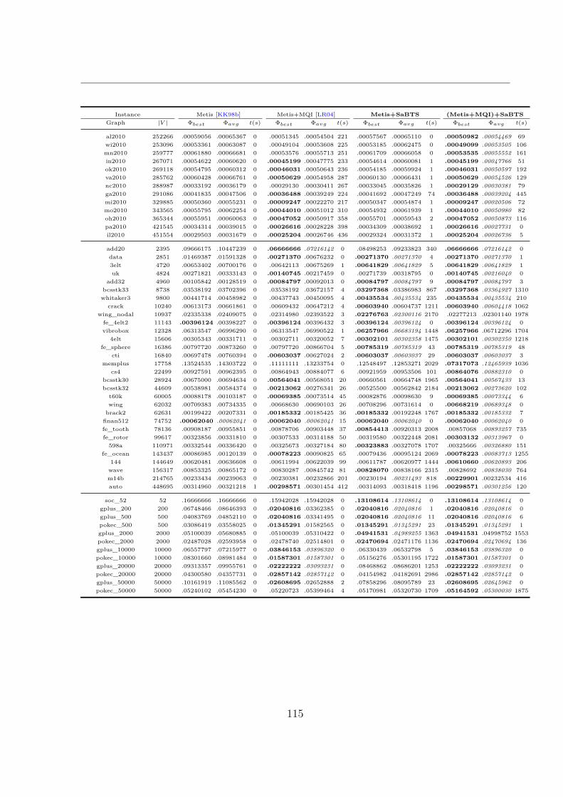
Instance Metis [KK98b] Metis+MQI [LR04] Metis+SaBTS (Metis+MQI)+SaBTSGraph |V | Φbest Φavg t(s) Φbest Φavg t(s) Φbest Φavg t(s) Φbest Φavg t(s)
al2010 252266 .00059056 .00065367 0 .00051345 .00054504 221 .00057567 .00065110 0 .00050982 .00054469 69wi2010 253096 .00053361 .00063087 0 .00049104 .00053608 225 .00053185 .00062475 0 .00049099 .00053505 106mn2010 259777 .00061880 .00066681 0 .00053576 .00055713 251 .00061709 .00066058 0 .00053535 .00055552 161in2010 267071 .00054622 .00060620 0 .00045199 .00047775 233 .00054614 .00060081 1 .00045199 .00047766 51ok2010 269118 .00054795 .00060312 0 .00046031 .00050643 236 .00054185 .00059924 1 .00046031 .00050597 192va2010 285762 .00060428 .00066761 0 .00050629 .00054958 287 .00060130 .00066431 1 .00050629 .00054526 129nc2010 288987 .00033192 .00036179 0 .00029130 .00030411 267 .00033045 .00035826 1 .00029129 .00030381 79ga2010 291086 .00041835 .00047506 0 .00036488 .00039249 224 .00041692 .00047249 74 .00036488 .00039204 445mi2010 329885 .00050360 .00055231 0 .00009247 .00022270 217 .00050347 .00054874 1 .00009247 .00020506 72mo2010 343565 .00055795 .00062254 0 .00044010 .00051012 310 .00054932 .00061939 1 .00044010 .00050980 82oh2010 365344 .00055951 .00060063 0 .00047052 .00050917 358 .00055701 .00059543 2 .00047052 .00050873 116pa2010 421545 .00034314 .00039015 0 .00026616 .00028228 398 .00034309 .00038692 1 .00026616 .00027731 0il2010 451554 .00029503 .00031679 0 .00025204 .00026746 436 .00029324 .00031372 1 .00025204 .00026736 5
add20 2395 .09666175 .10447239 0 .06666666 .07216142 0 .08498253 .09233823 340 .06666666 .07216142 0data 2851 .01469387 .01591328 0 .00271370 .00676232 0 .00271370 .00271370 4 .00271370 .00271370 13elt 4720 .00653402 .00700176 0 .00642113 .00675269 1 .00641829 .00641829 5 .00641829 .00641829 1uk 4824 .00271821 .00333143 0 .00140745 .00217459 0 .00271739 .00318795 0 .00140745 .00216040 0
add32 4960 .00105842 .00128519 0 .00084797 .00092013 0 .00084797 .00084797 9 .00084797 .00084797 3bcsstk33 8738 .03538192 .03702396 0 .03538192 .03672157 4 .03297368 .03386983 867 .03297368 .03364927 1310whitaker3 9800 .00441714 .00458982 0 .00437743 .00450095 4 .00435534 .00435534 235 .00435534 .00435534 210crack 10240 .00613173 .00661861 0 .00609432 .00647212 4 .00603940 .00604737 1211 .00603940 .00604418 1062
wing_nodal 10937 .02335338 .02409075 0 .02314980 .02393522 3 .02276763 .02300116 2170 .02277213 .02301140 1978fe_4elt2 11143 .00396124 .00398227 0 .00396124 .00396432 3 .00396124 .00396124 0 .00396124 .00396124 0vibrobox 12328 .06313547 .06996290 0 .06313547 .06990522 1 .06257966 .06683194 1448 .06257966 .06712296 1704
4elt 15606 .00305343 .00331711 0 .00302711 .00320052 7 .00302101 .00302358 1475 .00302101 .00302350 1218fe_sphere 16386 .00797720 .00873260 0 .00797720 .00866704 5 .00785319 .00785319 43 .00785319 .00785319 48
cti 16840 .00697478 .00760394 0 .00603037 .00627024 2 .00603037 .00603037 29 .00603037 .00603037 3memplus 17758 .13524535 .14303722 0 .11111111 .13233754 0 .12548497 .12853271 2029 .07317073 .12465939 1036
cs4 22499 .00927591 .00962395 0 .00864943 .00884077 6 .00921959 .00953506 101 .00864076 .00882310 0bcsstk30 28924 .00675000 .00694634 0 .00564041 .00568051 20 .00660561 .00664748 1965 .00564041 .00567433 13bcsstk32 44609 .00538981 .00584374 0 .00213062 .00276341 26 .00525500 .00562842 2184 .00213062 .00273620 102t60k 60005 .00088178 .00103187 0 .00069385 .00073514 45 .00082876 .00098630 9 .00069385 .00073344 6wing 62032 .00709383 .00734335 0 .00668630 .00690103 26 .00708296 .00731614 0 .00668219 .00689348 0brack2 62631 .00199422 .00207331 0 .00185332 .00185425 36 .00185332 .00192248 1767 .00185332 .00185332 7finan512 74752 .00062040 .00062041 0 .00062040 .00062041 15 .00062040 .00062040 0 .00062040 .00062040 0fe_tooth 78136 .00908187 .00955851 0 .00878706 .00903448 37 .00854413 .00920313 2008 .00857068 .00893257 735fe_rotor 99617 .00323856 .00331810 0 .00307533 .00314188 50 .00319580 .00322448 2081 .00303132 .00313967 0598a 110971 .00332544 .00336420 0 .00325673 .00327184 80 .00323883 .00327078 1707 .00325666 .00326880 151
fe_ocean 143437 .00086985 .00120139 0 .00078223 .00090825 65 .00079436 .00095124 2069 .00078223 .00083713 1255144 144649 .00620481 .00636608 0 .00611994 .00622039 99 .00611787 .00620977 1444 .00610660 .00620893 206wave 156317 .00853325 .00865172 0 .00830287 .00845742 81 .00828070 .00838166 2315 .00828692 .00838030 764m14b 214765 .00233434 .00239063 0 .00230381 .00232866 201 .00230194 .00231493 818 .00229901 .00232534 416auto 448695 .00314960 .00321218 1 .00298571 .00301454 412 .00314093 .00318418 1196 .00298571 .00301256 120
soc_52 52 .16666666 .16666666 0 .15942028 .15942028 0 .13108614 .13108614 0 .13108614 .13108614 0gplus_200 200 .06748466 .08646393 0 .02040816 .03362385 0 .02040816 .02040816 1 .02040816 .02040816 0gplus_500 500 .04083769 .04852110 0 .02040816 .03341495 0 .02040816 .02040816 11 .02040816 .02040816 6pokec_500 500 .03086419 .03558025 0 .01345291 .01582565 0 .01345291 .01345291 23 .01345291 .01345291 1gplus_2000 2000 .05100039 .05680885 0 .05100039 .05310422 0 .04941531 .04989255 1363 .04941531 .04998752 1553pokec_2000 2000 .02487028 .02593958 0 .02478740 .02514801 0 .02470694 .02471176 1136 .02470694 .02470694 136gplus_10000 10000 .06557797 .07215977 0 .03846153 .03896320 0 .06330439 .06532798 5 .03846153 .03896320 0pokec_10000 10000 .08301660 .08981484 0 .01587301 .01587301 0 .05156276 .05301195 1722 .01587301 .01587301 0gplus_20000 20000 .09313357 .09955761 0 .02222222 .03093231 0 .08468862 .08686201 1253 .02222222 .03093231 0pokec_20000 20000 .04300580 .04357731 0 .02857142 .02857142 0 .04154982 .04182691 2986 .02857142 .02857142 0gplus_50000 50000 .10161919 .11085562 0 .02608695 .02652888 2 .07858296 .08095789 23 .02608695 .02645962 0pokec_50000 50000 .05240102 .05454230 0 .05220723 .05399464 4 .05170981 .05320730 1709 .05164592 .05300030 1875
115
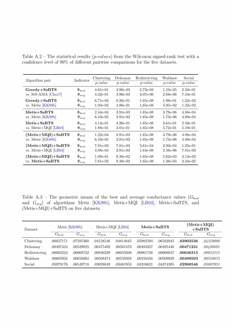
Table A.2 – The statistical results (p-values) from the Wilcoxon signed-rank test with aconfidence level of 99% of different pairwise comparisons for the five datasets.
Algorithm pair Indicator Clustering Delaunay Redistricting Walshaw Socialp-value p-value p-value p-value p-value
Greedy+SaBTSvs. StS-AMA [Cha17]
Φbest 4.61e-01 3.90e-03 2.73e-08 1.10e-05 2.50e-01Φavg 4.32e-01 3.90e-03 4.07e-06 2.88e-06 7.34e-01
Greedy+SaBTSvs. Metis [KK98b]
Φbest 6.71e-03 8.20e-01 1.65e-08 1.98e-01 1.22e-02Φavg 1.03e-02 4.96e-01 1.65e-08 4.95e-02 1.22e-02
Metis+SaBTSvs. Metis [KK98b]
Φbest 2.44e-04 3.91e-03 1.65e-08 3.79e-06 4.88e-04Φavg 6.10e-05 3.91e-03 1.65e-08 1.73e-06 4.88e-04
Metis+SaBTSvs. Metis+MQI [LR04]
Φbest 4.14e-01 4.26e-01 1.65e-08 3.61e-01 2.50e-01Φavg 1.88e-01 3.01e-01 1.65e-08 5.72e-01 5.19e-01
(Metis+MQI)+SaBTSvs. Metis [KK98b]
Φbest 1.22e-04 3.91e-03 1.65e-08 3.79e-06 4.88e-04Φavg 6.10e-05 3.91e-03 1.65e-08 1.73e-06 4.88e-04
(Metis+MQI)+SaBTSvs. Metis+MQI [LR04]
Φbest 7.81e-03 7.81e-03 3.61e-04 2.93e-04 1.25e-01Φavg 4.88e-04 3.91e-03 1.64e-08 2.56e-06 7.81e-03
(Metis+MQI)+SaBTSvs. Metis+SaBTS
Φbest 1.09e-01 9.38e-02 1.65e-08 5.62e-03 3.13e-02Φavg 7.81e-02 9.38e-02 1.65e-08 1.38e-03 2.34e-02
Table A.3 – The geometric means of the best and average conductance values (Gbest
and Gavg) of algorithms Metis [KK98b], Metis+MQI [LR04], Metis+SaBTS, and(Metis+MQI)+SaBTS on five datasets.
Dataset Metis [KK98b] Metis+MQI [LR04] Metis+SaBTS (Metis+MQI)+SaBTS
Gbest Gavg Gbest Gavg Gbest Gavg Gbest Gavg
Clustering .06627171 .07595360 .04158546 .04814845 .05982594 .06583945 .03902536 .04359008Delaunay .00497424 .00529025 .00475492 .00501473 .00483327 .00495440 .00471231 .00480691Redistricting .00062224 .00069732 .00046329 .00053508 .00061756 .00069047 .00046315 .00053315Walshaw .00605934 .00650062 .00509474 .00559503 .00550456 .00569929 .00499503 .00528675Social .05979176 .06549718 .03028849 .03461953 .04316621 .04374305 .02968546 .03067951
LIST OF FIGURES
1.1 An illustrative example for MC-GPP. . . . . . . . . . . . . . . . . . . . . . 18
2.1 An example of moving “non-critical” or “ordinary” vertices in the con-strained neighboring structure defined in the cut edges set. . . . . . . . . . 36
2.2 Analysis of the effects of the parameters (α, D, T , L0 and P0) on theperformance of the proposed SaBTS algorithm. . . . . . . . . . . . . . . . 50
3.1 The double-point crossover. . . . . . . . . . . . . . . . . . . . . . . . . . . 59
3.2 Performance profiles of the proposed MAMC algorithm and the four refer-ence algorithms Metis [KK98b], MQI [LR04], SaBTS [LHZ19], and MQI+SaBTS[LHZ19] on the two sets of 60 benchmark instances. . . . . . . . . . . . . 73
3.3 The communities detected by our proposed MAMC algorithm of the friend-ship network from Zachary’s karate club study. . . . . . . . . . . . . . . . 75
3.4 The communities of college football network. The colors indicate differentconferences, and clusterings for the communities identified by our proposedMAMC algorithm. . . . . . . . . . . . . . . . . . . . . . . . . . . . . . . . 76
3.5 The social network of 62 bottlenose dolphins. The nodes are colored basedon the groups observed in the study by Lusseau et al [Lus+03]. The clus-terings represent communities detected by our proposed MAMC algorithm. 77
3.6 Average values of Φbest and Φavg on six hard instances obtained by executingMAMC with different values of parameters α and d. . . . . . . . . . . . . . 78
3.7 Comparison of the quality-and-diversity based population initialization (de-noted by InitialMixed) with two random initialization variants (denoted byInitialRandom1 and InitialRandom2). . . . . . . . . . . . . . . . . . . . . . 79
3.8 Comparison of MAMC with the progressive constrained neighborhood (de-noted by PCNTS) and its variant with the whole neighborhood (denotedby CNTS) according to their running profiles (convergence graphs). . . . . 81
117

3.9 Comparison of the distance-and-quality based pool updating procedure (de-noted by PoolNew) and its variant only based on solution quality (denotedby PoolOld). . . . . . . . . . . . . . . . . . . . . . . . . . . . . . . . . . . . 82
4.1 An illustration of the iterated multilevel framework for the proposed IMSAalgorithm. . . . . . . . . . . . . . . . . . . . . . . . . . . . . . . . . . . . . 88
4.2 An example of the solution-guided coarsening process to create a coarsenedgraph. . . . . . . . . . . . . . . . . . . . . . . . . . . . . . . . . . . . . . . 90
4.3 Probability distributions of the time (in seconds) needed to attain a giventarget objective value by each reference algorithm on the 4 representativeinstances. . . . . . . . . . . . . . . . . . . . . . . . . . . . . . . . . . . . . 101
4.4 Comparisons of the proposed IMSA algorithm with a multi-start simulatedannealing plus tabu search (denoted by (SA+TS)restart) on 20 representa-tive instances. . . . . . . . . . . . . . . . . . . . . . . . . . . . . . . . . . . 103
4.5 Comparisons of the proposed IMSA algorithm with an IMSA variant wherethe SA-based local refinement is replaced by a descent search (denoted byIMSAdescent) on the 20 representative instances. . . . . . . . . . . . . . . . 104
4.6 Analysis of the parameters (ct, saIter, θ, ar, D, α) of the proposed IMSAalgorithm on its performance of the proposed IMSA algorithm. . . . . . . . 105
118
LIST OF TABLES
1.1 Summary of the key features and technical contributions of the most relatedstudies for MC-GPP. . . . . . . . . . . . . . . . . . . . . . . . . . . . . . . 22
1.2 Benchmark instances from “The 10th DIMACS Implementation ChallengeBenchmark” for MC-GPP: Part 1. This set includes 138 graphs which areclassified into 9 groups by their applications. Within each group, the in-stances are sorted by the number of vertices. . . . . . . . . . . . . . . . . . 26
1.3 Benchmark instances from “The 10th DIMACS Implementation ChallengeBenchmark” for MC-GPP: Part 2. This set includes 138 graphs which areclassified into 9 groups by their applications. Within each group, the in-stances are sorted by the number of vertices. . . . . . . . . . . . . . . . . . 27
1.4 Benchmark instances from the popular SNAP collection named by So-cial networks (left, 12 graphs) and “The Network Data Repository online”(right, 10 graphs) for MC-GPP. Within each set, the instances are sortedby the number of vertices. . . . . . . . . . . . . . . . . . . . . . . . . . . . 28
2.1 Parameter setting of the proposed SaBTS algorithm. . . . . . . . . . . . . 422.2 Comparative results of Greedy+SaBTS (when it is run with greedy ini-
tial solutions) with two reference algorithms StS-AMA [Cha17] and Metis[KK98b]. . . . . . . . . . . . . . . . . . . . . . . . . . . . . . . . . . . . . . 46
2.3 Comparative results of howMQI [LR04], SaBTS, and a combination of MQI[LR04] and SaBTS can improve the results of Metis [KK98b] (indicated byMetis+MQI, Metis+SaBTS and (Metis+MQI)+SaBTS respectively). . . . 47
2.4 Comparative results of how SaBTS can further improve the results ofMetis+MQI [LR04] (indicated by (Metis+MQI)+SaBTS). . . . . . . . . . 48
2.5 Comparison of SaBTS with a variant SaBTSno_cons using the unconstrainedneighborhood. . . . . . . . . . . . . . . . . . . . . . . . . . . . . . . . . . . 52
2.6 Comparison of SaBTS with three variants SaBTSD3, SaBTSD1+D2 andSaBTSD2+D3 applying different perturbation schemes. . . . . . . . . . . . . 53
119
3.1 Parameter setting of the proposed MAMC algorithm. . . . . . . . . . . . . 663.2 Detailed computational results of MAMC with two reference state-of-the-
art algorithms Metis [KK98b], MQI [LR04] on 50 large graphs from “The10th DIMACS Implementation Challenge Benchmark” and 10 large graphsfrom “The Network Data Repository online”. . . . . . . . . . . . . . . . . . 69
3.3 Detailed computational results of MAMC with two reference state-of-the-art algorithms SaBTS [LHZ19] and MQI+SaBTS [LHZ19] on 50 largegraphs from “The 10th DIMACS Implementation Challenge Benchmark”and 10 large graphs from “The Network Data Repository online”. . . . . . 71
3.4 Summary of comparative results between the proposed MAMC algorithmand each of the four reference algorithms Metis [KK98b], MQI [LR04],SaBTS [LHZ19], and MQI+SaBTS [LHZ19] on the two sets of 60 bench-mark instances. . . . . . . . . . . . . . . . . . . . . . . . . . . . . . . . . . 73
4.1 The parameter settings of the proposed IMSA algorithm. . . . . . . . . . . 954.2 Computational results on the 66 benchmark instances obtained by the
proposed IMSA algorithm and the three reference algorithms (MAMC[LHW20], SaBTS [LHZ19], and MQI [LR04]). . . . . . . . . . . . . . . . . 98
4.3 Summary results on the 66 benchmark instances reported by the proposedIMSA algorithm, and the three reference algorithms (MAMC [LHW20],SaBTS [LHZ19], and MQI [LR04]). . . . . . . . . . . . . . . . . . . . . . . 100
4.4 The geometric means of the best and the average conductance values (Gbest
and Gavg) reported by the IMSA algorithm, and the three reference algo-rithms (MAMC [LHW20], SaBTS [LHZ19], and MQI [LR04]) for the 66benchmark instances. . . . . . . . . . . . . . . . . . . . . . . . . . . . . . . 100
A.1 Detailed computational results of algorithms Metis [KK98b], Metis+MQI[LR04], Metis+SaBTS, and (Metis+MQI)+SaBTS on four datasets from“The 10th DIMACS Implementation Challenge Benchmark” (including 17Clustering, 9 Delaunay, 42 Redistricting, 30 Walshaw graphs) and 12 Socialnetwork graphs from the SNAP network dataset (a total of 110 graphs). . . 114
A.2 The statistical results (p-values) from the Wilcoxon signed-rank test with aconfidence level of 99% of different pairwise comparisons for the five datasets.116
A.3 The geometric means of the best and average conductance values (Gbest andGavg) of algorithms Metis [KK98b], Metis+MQI [LR04], Metis+SaBTS,and (Metis+MQI)+SaBTS on five datasets. . . . . . . . . . . . . . . . . . 116
120
LIST OF ALGORITHMS
1 Main framework of the stagnation-aware breakout tabu search (SaBTS) forMC-GPP. . . . . . . . . . . . . . . . . . . . . . . . . . . . . . . . . . . . . 32
2 Constrained neighborhood tabu search (CNTS). . . . . . . . . . . . . . . . 343 The self-adaptive perturbation procedure (SAP). . . . . . . . . . . . . . . . 404 Main framework of the memetic algorithm (MAMC) for MC-GPP. . . . . . 575 The quality-and-diversity based population initialization. . . . . . . . . . . 586 Progressive constrained neighborhood tabu search (PCNTS). . . . . . . . . 607 The distance-and-quality based updating procedure. . . . . . . . . . . . . . 648 Main framework of the iterated multilevel simulated annealing (IMSA) for
MC-GPP. . . . . . . . . . . . . . . . . . . . . . . . . . . . . . . . . . . . . 879 Simulated annealing based local refinement. . . . . . . . . . . . . . . . . . 91
121

LIST OF PUBLICATIONS
Published journal papers
- Zhi Lu, Jin-Kao Hao, Yi Zhou. Stagnation-aware breakout tabu search for the min-imum conductance graph partitioning problem. Computers & Operations Research111: 43-57, 2019.
- Zhi Lu, Jin-Kao Hao, Qinghua Wu. A hybrid evolutionary algorithm for finding lowconductance of large graphs. Future Generation Computer Systems 106: 105-120,2020.
Submitted journal papers
- Zhi Lu, Yi Zhou, Jin-Kao Hao. A hybrid evolutionary algorithm for the clique par-titioning problem. Submitted to IEEE Transactions on Cybernetics, Under review,March, 2020.
- Zhi Lu, Jin-Kao Hao, Una Benlic, David Lesaint. Iterated multilevel simulatedannealing for large-scale graph conductance minimization. Submitted to EuropeanJournal of Operational Research, Under review, May, 2020.
123

REFERENCES
[ARR07] Renata M Aiex, Mauricio GC Resende, and Celso C Ribeiro, « TTT plots:a perl program to create time-to-target plots », in: Optimization Letters 1.4(2007), pp. 355–366 (cit. on p. 100).
[AL08] Reid Andersen and Kevin J Lang, « An algorithm for improving graph parti-tions », in: Proceedings of the nineteenth annual ACM-SIAM symposium onDiscrete algorithms, Society for Industrial and Applied Mathematics, 2008,pp. 651–660 (cit. on pp. 20, 22, 43, 65).
[AHK04] Sanjeev Arora, Elad Hazan, and Satyen Kale, « O(√logn) Approximation
to Sparsest Cut in O(n2) Time », in: Proceedings of the 45th Annual IEEESymposium on Foundations of Computer Science, 2004, pp. 238–247 (cit. onpp. 19, 22).
[ARV09] Sanjeev Arora, Satish Rao, and Umesh Vazirani, « Expander flows, geometricembeddings and graph partitioning », in: Journal of the ACM (JACM) 56.2(2009), pp. 1–37 (cit. on pp. 19, 22).
[Bad+14] David A. Bader, Henning Meyerhenke, Peter Sanders, Christian Schulz, An-drea Kappes, and Dorothea Wagner, « Benchmarking for Graph Clusteringand Partitioning », in: Encyclopedia of Social Network Analysis and Mining,New York, NY: Springer New York, 2014, pp. 73–82 (cit. on pp. 23, 42, 65,94).
[Bad+13] David A. Bader, Henning Meyerhenke, Peter Sanders, and Dorothea Wagner,eds., Graph Partitioning and Graph Clustering, 10th DIMACS Implemen-tation Challenge Workshop, Georgia Institute of Technology, Atlanta, GA,USA, February 13-14, 2012. Proceedings, vol. 588, Contemporary Mathemat-ics, American Mathematical Society, 2013 (cit. on pp. 23, 42, 65, 94).
[BS94] Stephen T Barnard and Horst D Simon, « Fast multilevel implementationof recursive spectral bisection for partitioning unstructured problems », in:Concurrency: Practice and Experience 6.2 (1994), pp. 101–117 (cit. on pp. 85,86).
125
[BH11a] Una Benlic and Jin-Kao Hao, « A multilevel memetic approach for improvinggraph k-partitions », in: IEEE Transactions on Evolutionary Computation15.5 (2011), pp. 624–642 (cit. on pp. 56, 85, 86).
[BH11b] Una Benlic and Jin-Kao Hao, « An effective multilevel tabu search approachfor balanced graph partitioning », in: Computers & Operations Research 38.7(2011), pp. 1066–1075 (cit. on p. 34).
[BH13a] Una Benlic and Jin-Kao Hao, « Breakout local search for the max-cut prob-lem », in: Engineering Applications of Artificial Intelligence 26.3 (2013),pp. 1162–1173 (cit. on pp. 29, 30, 41).
[BH13b] Una Benlic and Jin-Kao Hao, « Breakout local search for the quadratic as-signment problem », in: Applied Mathematics and Computation 219.9 (2013),pp. 4800–4815 (cit. on pp. 29, 30, 41).
[BH13c] Una Benlic and Jin-Kao Hao, « Breakout local search for the vertex separa-tor problem », in: Twenty-Third International Joint Conference on ArtificialIntelligence, 2013 (cit. on pp. 29, 30, 41).
[BH13d] Una Benlic and Jin-Kao Hao, « Hybrid metaheuristics for the graph partition-ing problem », in: Hybrid Metaheuristics, Springer, 2013, pp. 157–185 (cit. onpp. 21, 38).
[BH15] Una Benlic and Jin-Kao Hao, « Memetic search for the quadratic assignmentproblem », in: Expert Systems with Applications 42.1 (2015), pp. 584–595(cit. on p. 56).
[BGL16] Austin R Benson, David F Gleich, and Jure Leskovec, « Higher-order organi-zation of complex networks », in: Science 353.6295 (2016), pp. 163–166 (cit.on p. 74).
[Bop87] Ravi B Boppana, « Eigenvalues and graph bisection: An average-case analy-sis », in: 28th Annual Symposium on Foundations of Computer Science (sfcs1987), IEEE, 1987, pp. 280–285 (cit. on p. 15).
[BJ93] Thang Nguyen Bui and Curt Jones, « A heuristic for reducing fill-in in sparsematrix factorization », in: Proceedings of the Sixth SIAM Conference on Par-allel Processing for Scientific Computing, 1993, pp. 445–452 (cit. on pp. 85,86).
126

[Bul+16] Aydın Buluç, Henning Meyerhenke, Ilya Safro, Peter Sanders, and ChristianSchulz, « Recent advances in graph partitioning », in: Algorithm Engineering,Springer, 2016, pp. 117–158 (cit. on pp. 21, 38).
[CKM00] Andrew E Caldwell, Andrew B Kahng, and Igor L Markov, « Design andimplementation of move-based heuristics for VLSI hypergraph partitioning »,in: Journal of Experimental Algorithmics (JEA) 5 (2000), 5–es (cit. on p. 42).
[Cha17] David Chalupa, « A memetic algorithm for the minimum conductance graphpartitioning problem », in: arXiv preprint arXiv:1704.02854 (2017) (cit. onpp. 21, 22, 24, 29, 31, 38, 42, 43, 46, 54, 61, 62, 93, 109, 116).
[CHW18] David Chalupa, Ken A Hawick, and James A Walker, « Hybrid bridge-basedmemetic algorithms for finding bottlenecks in complex networks », in: BigData Research 14 (2018), pp. 68–80 (cit. on pp. 17, 18, 21, 29, 74, 109).
[CLA12] Siew Yin Chan, Teck Chaw Ling, and Eric Aubanel, « The impact of hetero-geneous multi-core clusters on graph partitioning: an empirical study », in:Cluster Computing 15.3 (2012), pp. 281–302 (cit. on p. 24).
[Che69] Jeff Cheeger, « A lower bound for the smallest eigenvalue of the Laplacian »,in: Proceedings of the Princeton conference in honor of Professor S. Bochner,1969, pp. 195–199 (cit. on pp. 16, 19, 22).
[Che+06] David Cheng, Ravi Kannan, Santosh Vempala, and Grant Wang, « A divide-and-merge methodology for clustering », in: ACM Transactions on DatabaseSystems (TODS) 31.4 (2006), pp. 1499–1525 (cit. on p. 17).
[DM02] Elizabeth D Dolan and Jorge J Moré, « Benchmarking optimization soft-ware with performance profiles », in: Mathematical programming 91.2 (2002),pp. 201–213 (cit. on p. 68).
[FW86] Philip J Fleming and John J Wallace, « How not to lie with statistics: thecorrect way to summarize benchmark results », in: Communications of theACM 29.3 (1986), pp. 218–221 (cit. on pp. 44, 113).
[For10] Santo Fortunato, « Community detection in graphs », in: Physics reports486.3-5 (2010), pp. 75–174 (cit. on p. 17).
[GBF11] Philippe Galinier, Zied Boujbel, and Michael Coutinho Fernandes, « An effi-cient memetic algorithm for the graph partitioning problem », in: Annals ofOperations Research 191.1 (2011), pp. 1–22 (cit. on pp. 39, 56, 63, 66).
127

[GJ79] Michael R. Garey and David S. Johnson, Computers and Intractability: AGuide to the Theory of NP-Completeness, USA: W. H. Freeman & Company,New York, 1979 (cit. on p. 16).
[GN02] Michelle Girvan and Mark EJ Newman, « Community structure in social andbiological networks », in: Proceedings of the national academy of sciences99.12 (2002), pp. 7821–7826 (cit. on p. 74).
[GL97] Fred Glover and Manuel Laguna, Tabu Search, USA: Kluwer Academic Pub-lishers, 1997 (cit. on pp. 33, 34).
[GLJ19] Carlos Guerrero, Isaac Lera, and Carlos Juiz, « Evaluation and efficiency com-parison of evolutionary algorithms for service placement optimization in fogarchitectures », in: Future Generation Computer Systems 97 (2019), pp. 131–144 (cit. on p. 56).
[Gus02] Dan Gusfield, « Partition-distance: A problem and class of perfect graphs aris-ing in clustering », in: Information Processing Letters 82.3 (2002), pp. 159–164 (cit. on p. 63).
[HHK97] Lars W Hagen, DJ-H Huang, and Andrew B Kahng, « On implementationchoices for iterative improvement partitioning algorithms », in: IEEE Trans-actions on Computer-Aided Design of Integrated Circuits and Systems 16.10(1997), pp. 1199–1205 (cit. on p. 43).
[Hao12] Jin-Kao Hao, « Memetic algorithms in discrete optimization », in: Handbookof memetic algorithms, Springer, 2012, pp. 73–94 (cit. on p. 59).
[HB97] Scott Hauck and Gaetano Borriello, « An evaluation of bipartitioning tech-niques », in: IEEE Transactions on Computer-Aided Design of Integrated Cir-cuits and Systems 16.8 (1997), pp. 849–866 (cit. on pp. 44, 95, 113).
[HL95] Bruce Hendrickson and Robert W Leland, « A multi-level algorithm for par-titioning graphs. », in: Proceedings of the 1995 ACM/IEEE Conference onSupercomputing, 1995, p. 28 (cit. on pp. 85, 86).
[Heu10] Vincent Heuveline, « HiFlow3: A flexible and hardware-aware parallel finiteelement package », in: Proceedings of the 9th Workshop on Parallel/High-Performance Object-Oriented Scientific Computing, 2010, pp. 1–6 (cit. onp. 23).
128
[Hoc09] Dorit S Hochbaum, « Polynomial time algorithms for ratio regions and avariant of normalized cut », in: IEEE transactions on pattern analysis andmachine intelligence 32.5 (2009), pp. 889–898 (cit. on pp. 16, 19, 22).
[Hoc13] Dorit S Hochbaum, « A polynomial time algorithm for rayleigh ratio on dis-crete variables: Replacing spectral techniques for expander ratio, normalizedcut, and cheeger constant », in: Operations Research 61.1 (2013), pp. 184–198(cit. on pp. 19, 22).
[HSS10] Manuel Holtgrewe, Peter Sanders, and Christian Schulz, « Engineering a scal-able high quality graph partitioner », in: 2010 IEEE International Symposiumon Parallel & Distributed Processing (IPDPS), IEEE, 2010, pp. 1–12 (cit. onp. 23).
[KK98a] George Karypis and Vipin Kumar, « A fast and high quality multilevel schemefor partitioning irregular graphs », in: SIAM Journal on Scientific Computing20.1 (1998), pp. 359–392 (cit. on p. 89).
[KK98b] George Karypis and Vipin Kumar, « MeTiS 5.1.0: Unstructured Graphs Par-titioning and Sparse Matrix Ordering System », in: Technical Report, Depart-ment of Computer Science, University of Minnesota, 1998 (cit. on pp. 20, 29,31, 43, 46, 47, 54, 59, 65, 67, 69, 70, 73, 109, 113–116).
[KGV83] Scott Kirkpatrick, C Daniel Gelatt, and Mario P Vecchi, « Optimizationby simulated annealing », in: Science 220.4598 (1983), pp. 671–680 (cit. onp. 91).
[LR04] Kevin Lang and Satish Rao, « A flow-based method for improving the expan-sion or conductance of graph cuts », in: International Conference on IntegerProgramming and Combinatorial Optimization, Springer, 2004, pp. 325–337(cit. on pp. 20, 22, 29, 43, 47, 48, 54, 57, 58, 66, 67, 69, 70, 73, 83, 87, 94,98–100, 109, 110, 113–116).
[LR99] Tom Leighton and Satish Rao, « Multicommodity max-flow min-cut theoremsand their use in designing approximation algorithms », in: Journal of theACM (JACM) 46.6 (1999), pp. 787–832 (cit. on pp. 19, 22).
[LK14] Jure Leskovec and Andrej Krevl, SNAP Datasets: Stanford Large NetworkDataset Collection, http://snap.stanford.edu/data, June 2014 (cit. onp. 24).
129

[LK16] Jure Leskovec and Andrej Krevl, « SNAP datasets: Stanford large networkdataset collection (2014) », in: URL http://snap.stanford.edu/data (2016),p. 49 (cit. on p. 42).
[Les+08] Jure Leskovec, Kevin J Lang, Anirban Dasgupta, and Michael W Mahoney,« Statistical properties of community structure in large social and informationnetworks », in: Proceedings of the 17th international conference on WorldWide Web, 2008, pp. 695–704 (cit. on p. 17).
[Les+09] Jure Leskovec, Kevin J Lang, Anirban Dasgupta, and Michael W Mahoney,« Community structure in large networks: Natural cluster sizes and the ab-sence of large well-defined clusters », in: Internet Mathematics 6.1 (2009),pp. 29–123 (cit. on pp. 19, 22, 43, 66).
[LM17] Pan Li and Olgica Milenkovic, « Inhomogeneous hypergraph clustering withapplications », in: Advances in Neural Information Processing Systems, 2017,pp. 2308–2318 (cit. on p. 74).
[Lim+15] Yongsub Lim, Won Jo Lee, Ho Jin Choi, and U Kang, « Discovering largesubsets with high quality partitions in real world graphs », in: 2015 Interna-tional Conference on Big Data and Smart Computing (BIGCOMP), IEEE,2015, pp. 186–193 (cit. on pp. 20, 22).
[Lim+17] Yongsub Lim, Won Jo Lee, Ho Jin Choi, and U Kang, « MTP: discovering highquality partitions in real world graphs », in: World Wide Web 20.3 (2017),pp. 491–514 (cit. on pp. 20, 22).
[LWN18] Zhenqi Lu, Johan Wahlström, and Arye Nehorai, « Community detection incomplex networks via clique conductance », in: Scientific reports 8.1 (2018),pp. 1–16 (cit. on p. 74).
[LHW20] Zhi Lu, Jin Kao Hao, and Qinghua Wu, « A hybrid evolutionary algorithm forfinding low conductance of large graphs », in: Future Generation ComputerSystems 106 (2020), pp. 105–120 (cit. on pp. 11, 93–95, 98–100).
[LHZ19] Zhi Lu, Jin Kao Hao, and Yi Zhou, « Stagnation-aware breakout tabu searchfor the minimum conductance graph partitioning problem », in: Computers& Operations Research 111 (2019), pp. 43–57 (cit. on pp. 11, 59, 61–63, 66,67, 71–73, 93–95, 98–100).
130

[LGH10] Zhipeng Lü, Fred Glover, and Jin-Kao Hao, « A hybrid metaheuristic ap-proach to solving the UBQP problem », in: European Journal of OperationalResearch 207.3 (2010), pp. 1254–1262 (cit. on pp. 56, 63).
[Lus+03] David Lusseau, Karsten Schneider, Oliver J Boisseau, Patti Haase, Elisa-beth Slooten, and Steve M Dawson, « The bottlenose dolphin community ofDoubtful Sound features a large proportion of long-lasting associations », in:Behavioral Ecology and Sociobiology 54.4 (2003), pp. 396–405 (cit. on pp. 75,77).
[MS05] Oliver Marquardt and Stefan Schamberger, « Open Benchmarks for LoadBalancing Heuristics in Parallel Adaptive Finite Element Computations. »,in: PDPTA, 2005, pp. 685–691 (cit. on p. 24).
[MG18] Laurent Moalic and Alexandre Gondran, « Variations on memetic algorithmsfor graph coloring problems », in: Journal of Heuristics 24.1 (2018), pp. 1–24(cit. on p. 56).
[Mou+18] Douglas LL Moura, Raquel S Cabral, Thiago Sales, and Andre LL Aquino,« An evolutionary algorithm for roadside unit deployment with between-ness centrality preprocessing », in: Future Generation Computer Systems 88(2018), pp. 776–784 (cit. on p. 56).
[NCM11] Ferrante Neri, Carlos Cotta, and Pablo Moscato, Handbook of memetic algo-rithms, vol. 379, Springer, 2011 (cit. on p. 56).
[PHK10] Daniel Cosmin Porumbel, Jin-Kao Hao, and Pascale Kuntz, « An evolutionaryapproach with diversity guarantee and well-informed grouping recombinationfor graph coloring », in: Computers & Operations Research 37.10 (2010),pp. 1822–1832 (cit. on pp. 56, 63).
[RA15] Ryan A. Rossi and Nesreen K. Ahmed, « The Network Data Repositorywith Interactive Graph Analytics and Visualization », in: Proceedings of theTwenty-Ninth AAAI Conference on Artificial Intelligence, AAAI’15, Austin,Texas: AAAI Press, 2015, pp. 4292–4293 (cit. on pp. 24, 65, 94).
[SS16] Peter Sanders and Christian Schulz, « KaHIP–Karlsruhe High Quality Parti-tioning », in: URL http://algo2.iti.kit.edu/kahip/ (2016) (cit. on p. 31).
[Sch07] Satu Elisa Schaeffer, « Graph clustering », in: Computer science review 1.1(2007), pp. 27–64 (cit. on p. 17).
131

[SM00] Jianbo Shi and Jitendra Malik, « Normalized cuts and image segmentation »,in: IEEE Transactions on pattern analysis and machine intelligence 22.8(2000), pp. 888–905 (cit. on p. 18).
[ŠS06] Jiří Šíma and Satu Elisa Schaeffer, « On the NP-completeness of some graphcluster measures », in: International Conference on Current Trends in Theoryand Practice of Computer Science, Springer, 2006, pp. 530–537 (cit. on p. 16).
[SSS16] Abel Soares Siqueira, Raniere Costa da Silva, and Luiz-Rafael Santos, « Perprof-py: A python package for performance profile of mathematical optimizationsoftware », in: Journal of Open Research Software 4.1 (2016) (cit. on p. 68).
[SWC04] Alan J Soper, Chris Walshaw, and Mark Cross, « A combined evolution-ary search and multilevel optimisation approach to graph-partitioning », in:Journal of Global Optimization 29.2 (2004), pp. 225–241 (cit. on p. 23).
[ST13] Daniel A Spielman and Shang Hua Teng, « A local clustering algorithm formassive graphs and its application to nearly linear time graph partitioning »,in: SIAM Journal on computing 42.1 (2013), pp. 1–26 (cit. on pp. 17, 20, 22).
[Tey+17] Luan Teylo, Ubiratam de Paula, Yuri Frota, Daniel de Oliveira, and LúciaMA Drummond, « A hybrid evolutionary algorithm for task scheduling anddata assignment of data-intensive scientific workflows on clouds », in: FutureGeneration Computer Systems 76 (2017), pp. 1–17 (cit. on p. 56).
[TOS01] Ulrich Trottenberg, Cornelius W. Oosterlee, and Anton Schüller, Multigrid,Academic Press, London, 2001 (cit. on p. 86).
[Val+20] Alan Valejo, Vinícius Ferreira, Renato Fabbri, Maria Cristina Ferreira deOliveira, and Alneu de Andrade Lopes, « A Critical Survey of the MultilevelMethod in Complex Networks », in: ACM Computing Surveys (CSUR) 53.2(2020), pp. 1–35 (cit. on pp. 85, 86).
[VM16] Twan Van Laarhoven and Elena Marchiori, « Local network community de-tection with continuous optimization of conductance and weighted kernel k-means », in: The Journal of Machine Learning Research 17.1 (2016), pp. 5148–5175 (cit. on pp. 17, 20, 22).
[VTX09] Konstantin Voevodski, Shang-Hua Teng, and Yu Xia, « Finding local com-munities in protein networks », in: BMC bioinformatics 10.1 (2009), p. 297(cit. on pp. 17, 18).
132

[Wal04] Chris Walshaw, « Multilevel refinement for combinatorial optimisation prob-lems », in: Annals of Operations Research 131.1-4 (2004), pp. 325–372 (cit.on pp. 85, 86).
[WZ11] Markus Wittmann and Thomas Zeiser, « Data structures of ilbdc latticeboltzmann solver », in: (2011) (cit. on p. 23).
[WH13] Qinghua Wu and Jin-Kao Hao, « Memetic search for the max-bisection prob-lem », in: Computers & Operations Research 40.1 (2013), pp. 166–179 (cit. onpp. 39, 56, 63, 66).
[YL15] Jaewon Yang and Jure Leskovec, « Defining and evaluating network commu-nities based on ground-truth », in: Knowledge and Information Systems 42.1(2015), pp. 181–213 (cit. on pp. 17, 18).
[Zac77] Wayne W Zachary, « An information flow model for conflict and fission insmall groups », in: Journal of anthropological research 33.4 (1977), pp. 452–473 (cit. on p. 74).
[ZLM13] Zeyuan Allen Zhu, Silvio Lattanzi, and Vahab S Mirrokni, « A Local Algo-rithm for Finding Well-Connected Clusters. », in: ICML (3), 2013, pp. 396–404 (cit. on pp. 17, 20, 22).
133


Titre : Approches d’Optimisation pour le Partitionnement de Graphede Conductance Minimale
Mot clés : Minimisation de la conductance, Partitionnement de graphes, Optimisation combi-
natoire, Métaheuristiques, Recherche de voisinage, Algorithme hybride, Multiniveaux, Optimi-
sation de grands graphes.
Résumé : Le problème de partitionnementde graphe de conductance minimale (MC-GPP) est un problème d’optimisation combi-natoire NP-difficile avec de nombreuses ap-plications pratiques dans divers domainestels que la détection communautaire, labioinformatique et la vision par ordinateur.Etant donnée sa complexité intrinsèque, desapproches heuristiques et métaheuristiquesconstituent un moyen convenable pour ré-soudre des instances de grande taille. Cettethèse est consacrée au développement d’al-gorithmes métaheuristiques performants pourle MC-GPP. Plus précisément, nous propo-
sons un algorithme «Stagnation aware Brea-kout Tabu Search», un algorithme évolutif hy-bride (MAMC) et un algorithme multiniveaubasé sur le recuit simulé (IMSA). Nous pré-sentons des résultats expérimentaux sur denombreux graphes de grande dimension dela littérature ayant jusqu’à 23 millions de som-mets. Nous montrons la haute performance denos algorithmes par rapport à l’état de l’art.Nous analysons les éléments algorithmiqueset stratégies de recherche pour mettre en lu-mière leur influence sur la performance des al-gorithmes proposés.
Title : Optimization Approaches for Minimum Conductance GraphPartitioning
Keywords : Conductance minimization, Graph partitioning, Combinatorial optimization, Meta-
heuristics, Neighborhood search, Hybrid algorithm, Multilevel, Large graph optimization.
Abstract : The minimum conductance graphpartitioning problem (MC-GPP) is an importantNP-hard combinatorial optimization problemwith numerous practical applications in variousareas such as community detection, bioinfor-matics, and computer vision. Due to its highcomputational complexity, heuristic and meta-heuristic approaches constitute a highly use-ful tool for approximating this challenging prob-lem. This thesis is devoted to developing effec-tive metaheuristic algorithms for the MC-GPP.Specifically, we propose a stagnation-aware
breakout tabu search algorithm (SaBTS), a hy-brid evolutionary algorithm (MAMC), and aniterated multilevel simulated annealing algo-rithm (IMSA). Extensive computational experi-ments and comparisons on large and massivebenchmark instances (with more than 23 mil-lion vertices) demonstrate that the proposedalgorithms compete very favorably with state-of-the-art algorithms in the literature. Further-more, the key issues of these algorithms areanalyzed to shed light on their influences overthe performance of the proposed algorithms.