Beyond-All-Orders Instability in the Equatorial

Kelvin Wave

Andrei Natarov

John P. Boyd

Department of Atmospheric, Oceanicand Space Science and Laboratory for Scientific Computation,

University of Michigan, 2455 Hayward Avenue, Ann Arbor MI 48109jpboyd@engin.umich.edu;

http://www.engin.umich.edu:/∼ jpboyd/

August 24, 2000

Dynamics of Atmospheres and Oceans, in press.

1

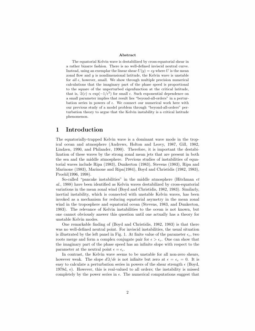
Abstract

The equatorial Kelvin wave is destabilized by cross-equatorial shear ina rather bizarre fashion. There is no well-defined inviscid neutral curve.Instead, using an exemplar the linear shear U(y) = εy where U is the meanzonal flow and y is nondimensional latitude, the Kelvin wave is unstablefor all ε, however, small. We show through multiple precision numericalcalculations that the imaginary part of the phase speed is proportionalto the square of the unperturbed eigenfunction at the critical latitude,that is, =(c) ∝ exp(−1/ε2) for small ε. Such exponential dependence ona small parameter implies that result lies “beyond-all-orders” in a pertur-bation series in powers of ε. We connect our numerical work here withour previous study of a model problem through “beyond-all-orders” per-turbation theory to argue that the Kelvin instability is a critical latitudephenomenon.

1 Introduction

The equatorially-trapped Kelvin wave is a dominant wave mode in the trop-ical ocean and atmosphere (Andrews, Holton and Leovy, 1987, Gill, 1982,Lindzen, 1990, and Philander, 1990). Therefore, it is important the destabi-lization of these waves by the strong zonal mean jets that are present in boththe sea and the middle atmosphere. Previous studies of instabilities of equa-torial waves include Ripa (1983), Dunkerton (1983), Stevens (1983), Ripa andMarinone (1983), Marinone and Ripa(1984), Boyd and Christidis (1982, 1983),Proehl(1996, 1998).

So-called “pancake instabilities” in the middle atmosphere (Hitchman etal., 1988) have been identified as Kelvin waves destabilized by cross-equatorialvariations in the mean zonal wind (Boyd and Christidis, 1982, 1983). Similarly,inertial instability, which is connected with unstable Kelvin waves, has beeninvoked as a mechanism for reducing equatorial asymetry in the mean zonalwind in the troposphere and equatorial ocean (Stevens, 1983, and Dunkerton,1983). The relevance of Kelvin instabilities to the ocean is not known, butone cannot obviously answer this question until one actually has a theory forunstable Kelvin modes.

One remarkable finding of (Boyd and Christidis, 1982, 1983) is that therewas no well-defined neutral point. For inviscid instabilities, the usual situationis illustrated by the left panel in Fig. 1. At finite value of the parameter εc, tworoots merge and form a complex conjugate pair for ε > εc. One can show thatthe imaginary part of the phase speed has an infinite slope with respect to theparameter at the neutral point ε = εc.

In contrast, the Kelvin wave seems to be unstable for all non-zero shears,however weak. The slope d=/dε is not infinite but zero at ε = εc = 0. It iseasy to calculate a perturbation series in powers of the shear strength ε (Boyd,1978d, e). However, this is real-valued to all orders; the instability is missedcompletely by the power series in ε. The numerical computations suggest that

2

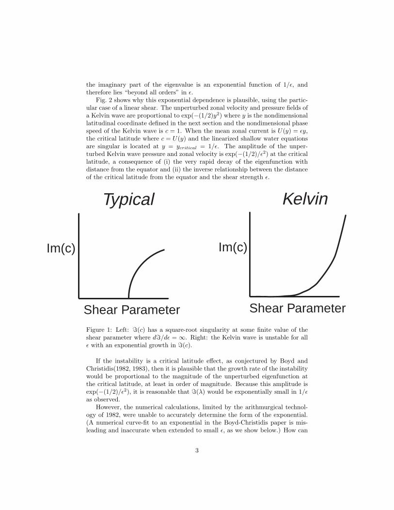
the imaginary part of the eigenvalue is an exponential function of 1/ε, andtherefore lies “beyond all orders” in ε.

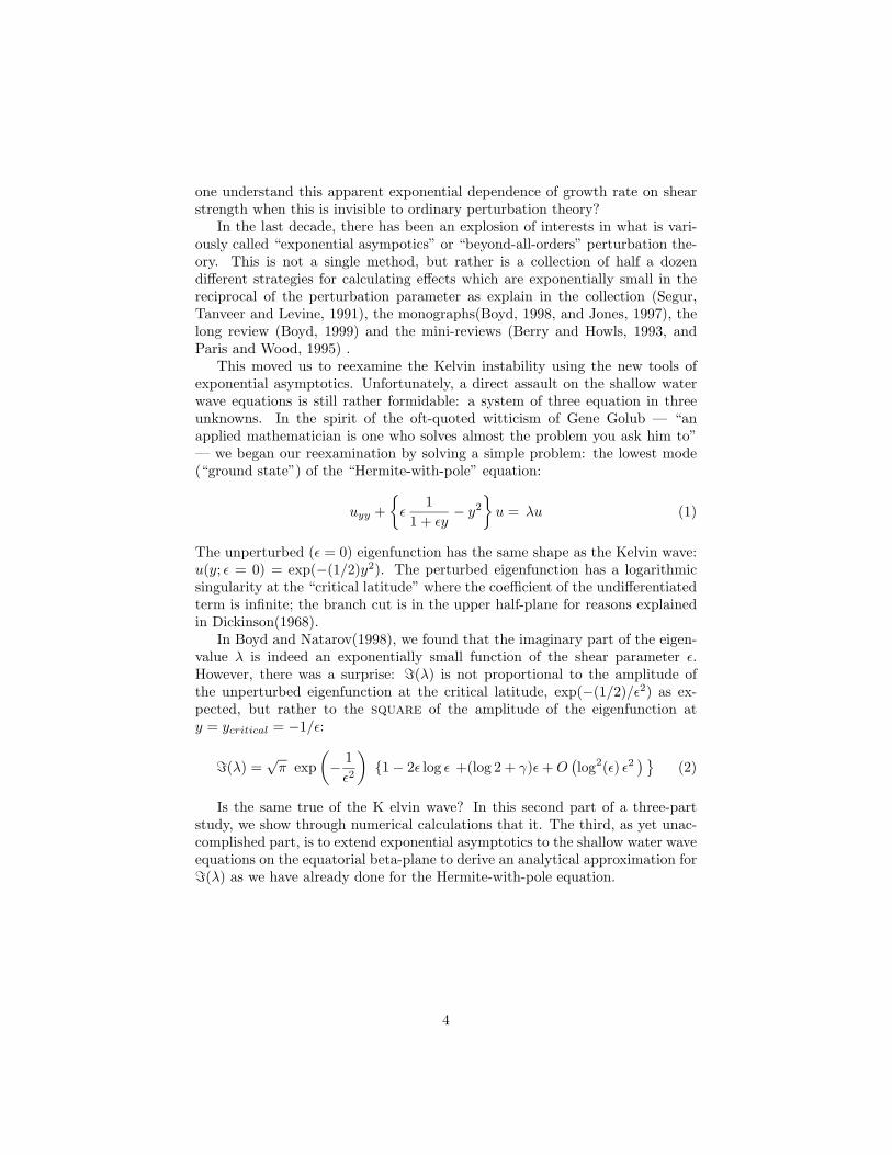
Fig. 2 shows why this exponential dependence is plausible, using the partic-ular case of a linear shear. The unperturbed zonal velocity and pressure fields ofa Kelvin wave are proportional to exp(−(1/2)y2) where y is the nondimensionallatitudinal coordinate defined in the next section and the nondimensional phasespeed of the Kelvin wave is c = 1. When the mean zonal current is U(y) = εy,the critical latitude where c = U(y) and the linearized shallow water equationsare singular is located at y = ycritical = 1/ε. The amplitude of the unper-turbed Kelvin wave pressure and zonal velocity is exp(−(1/2)/ε2) at the criticallatitude, a consequence of (i) the very rapid decay of the eigenfunction withdistance from the equator and (ii) the inverse relationship between the distanceof the critical latitude from the equator and the shear strength ε.

Shear Parameter Shear Parameter

Im(c) Im(c)

Typical Kelvin

Figure 1: Left: =(c) has a square-root singularity at some finite value of theshear parameter where d=/dε = ∞. Right: the Kelvin wave is unstable for allε with an exponential growth in =(c).

If the instability is a critical latitude effect, as conjectured by Boyd andChristidis(1982, 1983), then it is plausible that the growth rate of the instabilitywould be proportional to the magnitude of the unperturbed eigenfunction atthe critical latitude, at least in order of magnitude. Because this amplitude isexp(−(1/2)/ε2), it is reasonable that =(λ) would be exponentially small in 1/εas observed.

However, the numerical calculations, limited by the arithmurgical technol-ogy of 1982, were unable to accurately determine the form of the exponential.(A numerical curve-fit to an exponential in the Boyd-Christidis paper is mis-leading and inaccurate when extended to small ε, as we show below.) How can

3

one understand this apparent exponential dependence of growth rate on shearstrength when this is invisible to ordinary perturbation theory?

In the last decade, there has been an explosion of interests in what is vari-ously called “exponential asympotics” or “beyond-all-orders” perturbation the-ory. This is not a single method, but rather is a collection of half a dozendifferent strategies for calculating effects which are exponentially small in thereciprocal of the perturbation parameter as explain in the collection (Segur,Tanveer and Levine, 1991), the monographs(Boyd, 1998, and Jones, 1997), thelong review (Boyd, 1999) and the mini-reviews (Berry and Howls, 1993, andParis and Wood, 1995) .

This moved us to reexamine the Kelvin instability using the new tools ofexponential asymptotics. Unfortunately, a direct assault on the shallow waterwave equations is still rather formidable: a system of three equation in threeunknowns. In the spirit of the oft-quoted witticism of Gene Golub — “anapplied mathematician is one who solves almost the problem you ask him to”— we began our reexamination by solving a simple problem: the lowest mode(“ground state”) of the “Hermite-with-pole” equation:

uyy +{ε

11 + εy

− y2

}u = λu (1)

The unperturbed (ε = 0) eigenfunction has the same shape as the Kelvin wave:u(y; ε = 0) = exp(−(1/2)y2). The perturbed eigenfunction has a logarithmicsingularity at the “critical latitude” where the coefficient of the undifferentiatedterm is infinite; the branch cut is in the upper half-plane for reasons explainedin Dickinson(1968).

In Boyd and Natarov(1998), we found that the imaginary part of the eigen-value λ is indeed an exponentially small function of the shear parameter ε.However, there was a surprise: =(λ) is not proportional to the amplitude ofthe unperturbed eigenfunction at the critical latitude, exp(−(1/2)/ε2) as ex-pected, but rather to the square of the amplitude of the eigenfunction aty = ycritical = −1/ε:

=(λ) =√π exp

(− 1ε2

){1− 2ε log ε +(log 2 + γ)ε+O

(log2(ε) ε2

) }(2)

Is the same true of the K elvin wave? In this second part of a three-partstudy, we show through numerical calculations that it. The third, as yet unac-complished part, is to extend exponential asymptotics to the shallow water waveequations on the equatorial beta-plane to derive an analytical approximation for=(λ) as we have already done for the Hermite-with-pole equation.

4

-4 -2 0 2 40

0.5

1Kelvin eigenmode (u or height)

Crit

ical

Latit

ude

-4 -2 0 2 4-1

0

1

2

Crit

ical

Latit

ude

1/εy

c -

U(y

)

c ≈ 1, U ≡ ε y

Figure 2: Top: schematic of a linearized Kelvin wave in a mean shear flow.Bottom: graph of c − U(y) for the Kelvin wave for Couette flow, U(y) ≡ εy.The wave equation is singular, and the eigenmode has a critical latitude, aty = −1/ε where c − U is zero. The critical latitude creates an imaginary partin the phase speed c. However, =(c) is exponentially small in 1/ε2 because theamplitude of the eigenfunction at y = 1/ε is O(exp(−1/ε2)).

5

2 Numerical Solutions

The shallow water equations in a moving reference frame are

(u− c)ux + vuy − yv + hx = 0 (3)

(u− c)vx + vvy + yu+ hy = 0 (4)

{(u− c)h}x + {vh}y = 0 (5)

where c is the phase speed and h = 1+φ is the total depth. Linearization aboutthe basic state {u, v, φ} = {U(y), 0,Φ(y)} gives

(U − c)ux + vUy − yv + hx = 0 (6)

(U − c)vx + yu+ hy = 0 (7)

(U − c)hx + {1 + Φ}ux + {1 + Φ}vy + Φyv = 0 (8)

where the basic state is assumed to be geostrophically balanced.When the shallow water is derived by separating variables in the equations

of motion for a three-dimensional, compressible atmosphere, the result is iden-tical to the system except that in the continuously stratified case, Φ(y) ≡ 0 asexplained in Boyd and Christidis (1982, 1983). (Of course, the interpretation ofthe shallow water wave equations is changed, too: the three-dimensional wavemode is the product of factors that depend only on z times the solution of theshallow water set, which describes the latitude and longitude dependence of thewave.) For consistency with the earlier work, this is the set of equations we shallsolve below except for the computations of Table 3 where we compare Φ = 0with nonzero Φ.

Because the primary purpose of this work is to study critical latitude effectsin isolation from other possible forms of instability, we choose linear shear flowU(y) = εy as basic state for further studies. Such profile does not have singu-larities in the complex y-plane, which could complicate the numerics, or inflec-tion points. The only problem is that physically it cannot be supported by anygeostrophic Φ(y), because the streamlines would hit the surface (Φ(ysurf ) = −1)long before they reach critical latitude. This is a second reason to emphasizethe atmospheric model, Φ ≡ 0.

The search for normal mode solutions leads to a linear eigenvalue problemfor c ikU −y + ∂yU ik

y ikU ∂yik ∂y ikU

uvφ

= ikc

uvφ

(9)

6

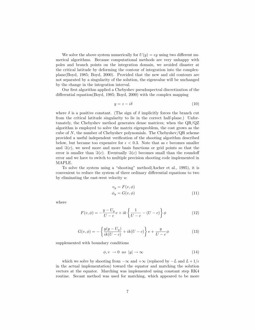
We solve the above system numerically for U(y) = εy using two different nu-merical algorithms. Because computational methods are very unhappy withpoles and branch points on the integration domain, we avoided disaster atthe critical latitude by deforming the contour of integration into the complex-plane(Boyd, 1985; Boyd, 2000). Provided that the new and old contours arenot separated by a singularity of the solution, the eigenvalue will be unchangedby the change in the integration interval.

Our first algorithm applied a Chebyshev pseudospectral discretization of thedifferential equation(Boyd, 1985; Boyd, 2000) with the complex mapping

y = z − iδ (10)

where δ is a positive constant. (The sign of δ implicitly forces the branch cutfrom the critical latitude singularity to lie in the correct half-plane.) Unfor-tunately, the Chebyshev method generates dense matrices; when the QR/QZalgorithm is employed to solve the matrix eigenproblem, the cost grows as thecube of N , the number of Chebyshev polynomials. The Chebyshev/QR schemeprovided a useful independent verification of the shooting algorithm describedbelow, but became too expensive for ε < 0.3. Note that as ε becomes smallerand =(c), we need more and more basis functions or grid points so that theerror is smaller than =(c). Eventually =(c) becomes small than the roundofferror and we have to switch to multiple precision shooting code implemented inMAPLE.

To solve the system using a “shooting” method(Ascher et al., 1995), it isconvenient to reduce the system of three ordinary differential equations to twoby eliminating the east-west velocity u:

vy = F (v, φ)φy = G(v, φ) (11)

where

F (v, φ) = −y − UyU − c v + ik

{1

U − c − (U − c)}φ (12)

G(v, φ) = −{y(y − Uy)ik(U − c) + ik(U − c)

}v +

y

U − cφ (13)

supplemented with boundary conditions

φ, v → 0 as |y| → ∞ (14)

which we solve by shooting from −∞ and +∞ (replaced by −L and L+ 1/εin the actual implementation) toward the equator and matching the solutionvectors at the equator. Marching was implemented using constant step RK4routine. Secant method was used for matching, which appeared to be more

7

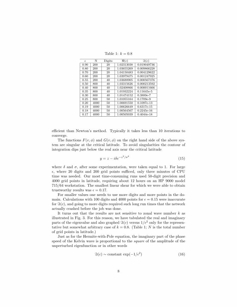
Table 1: k = 0.8

ε N Digits <(c) =(c)0.90 200 20 1.02313038 0.0190497360.80 200 20 1.03655269 0.0098662280.70 200 20 1.04150483 0.0041296220.60 200 20 1.03979475 0.0012479250.55 200 40 1.03688905 0.0005673760.50 800 40 1.03315626 0.0002135920.40 800 40 1.02408866 0.0000116660.35 800 40 1.01932224 0.11645e-50.30 800 40 1.01474152 0.3889e-70.25 800 50 1.01055164 0.1709e-90.20 4000 50 1.00691550 0.1097e-130.19 4000 50 1.00626649 0.6317e-150.18 4000 50 1.00564567 0.2245e-160.17 4000 50 1.00505039 0.4044e-18

efficient than Newton’s method. Typically it takes less than 10 iterations toconverge.

The functions F (v, φ) and G(v, φ) on the right hand side of the above sys-tem are singular at the critical latitude. To avoid singularities the contour ofintegration dips just below the real axis near the critical latitude

y = z − iδe−z2/σ2(15)

where δ and σ, after some experimentation, were taken equal to 1. For largeε, where 20 digits and 200 grid points sufficed, only three minutes of CPUtime was needed. Our most time-consuming runs used 50-digit precision and4000 grid points in latitude, requiring about 12 hours on an HP 9000 model715/64 workstation. The smallest linear shear for which we were able to obtaintrustworthy results was ε = 0.17.

For smaller values one needs to use more digits and more points in the do-main. Calculations with 100 digits and 4000 points for ε = 0.15 were inaccuratefor =(c), and going to more digits required such long run times that the networkactually crashed before the job was done.

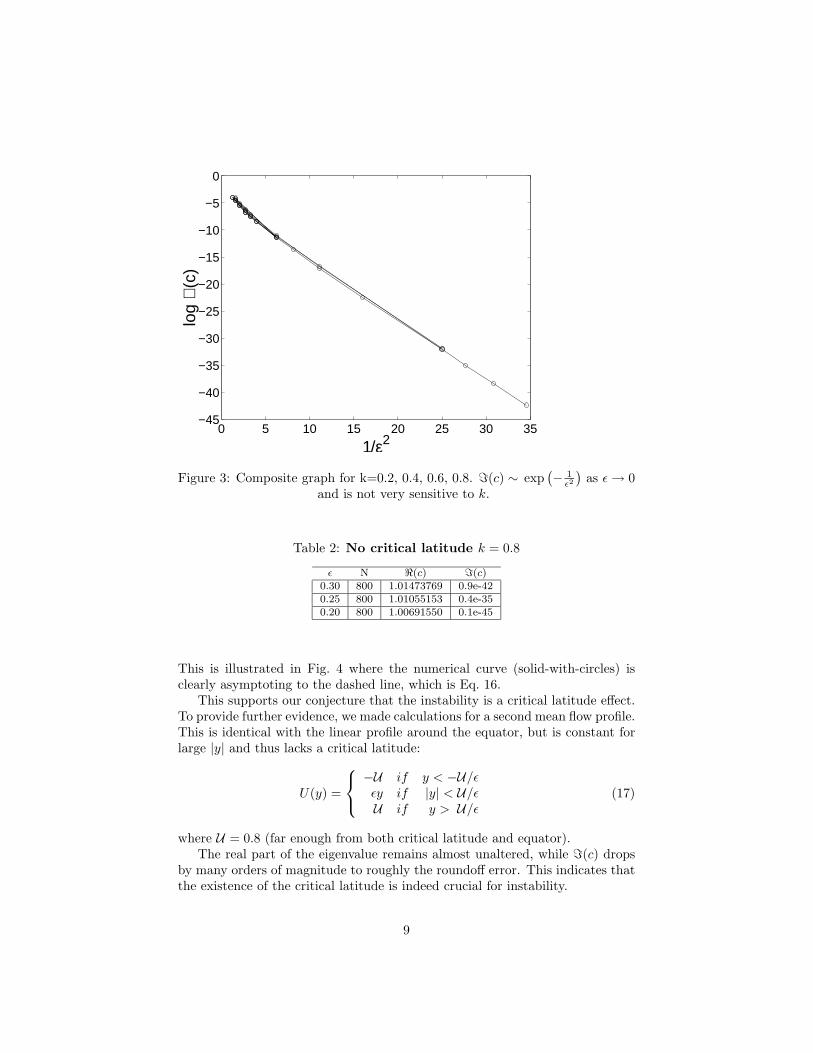
It turns out that the results are not sensitive to zonal wave number k asillustrated in Fig. 3. For this reason, we have tabulated the real and imaginaryparts of the eigenvalue and also graphed =(c) versus 1/ε2 only for the represen-tative but somewhat arbitrary case of k = 0.8. (Table 1; N is the total numberof grid points in latitude.)

Just as for the Hermite-with-Pole equation, the imaginary part of the phasespeed of the Kelvin wave is proportional to the square of the amplitude of theunperturbed eigenfunction or in other words

=(c) ∼ constant exp(−1/ε2) (16)

8

0 5 10 15 20 25 30 35−45

−40

−35

−30

−25

−20

−15

−10

−5

0

1/ε2

log

ℑ(c

)

Figure 3: Composite graph for k=0.2, 0.4, 0.6, 0.8. =(c) ∼ exp(− 1ε2

)as ε→ 0

and is not very sensitive to k.

Table 2: No critical latitude k = 0.8

ε N <(c) =(c)0.30 800 1.01473769 0.9e-420.25 800 1.01055153 0.4e-350.20 800 1.00691550 0.1e-45

This is illustrated in Fig. 4 where the numerical curve (solid-with-circles) isclearly asymptoting to the dashed line, which is Eq. 16.

This supports our conjecture that the instability is a critical latitude effect.To provide further evidence, we made calculations for a second mean flow profile.This is identical with the linear profile around the equator, but is constant forlarge |y| and thus lacks a critical latitude:

U(y) =

−U if y < −U/εεy if |y| < U/εU if y > U/ε

(17)

where U = 0.8 (far enough from both critical latitude and equator).The real part of the eigenvalue remains almost unaltered, while =(c) drops

by many orders of magnitude to roughly the roundoff error. This indicates thatthe existence of the critical latitude is indeed crucial for instability.

9

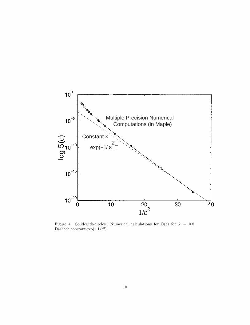
Multiple Precision Numerical Computations (in Maple)

Constant ×

exp(−1/ ε )2

Figure 4: Solid-with-circles: Numerical calculations for =(c) for k = 0.8.Dashed: constant exp(−1/ε2).

10

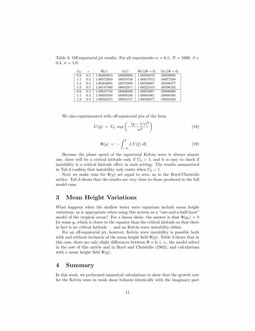
Table 3: Off-equatorial jet results. For all experiments w = 0.1, N = 1600, δ =0.4, σ = 1.0.

U0 ε <(c) =(c) <(c)[Φ = 0] =(c)[Φ = 0]0.9 0.5 1.00460854 .00000000 1.00508879 .000000001.1 0.5 1.00572669 .00078746 1.00617015 .000773981.2 0.5 1.00404085 .00373990 1.00508687 .003984771.3 0.5 1.00147460 .00642911 1.00223319 .005961920.9 0.4 1.00047156 .00000000 1.0005399? .000000001.1 0.4 1.00058580 .00008100 1.00064961 .000083061.2 0.4 1.00042015 .0003374? 1.00048877 .00032438

We also experimented with off-equatorial jets of the form

U(y) = U0 exp(− (y − 1/ε)2

w2

)(18)

Φ(y) = −∫ y

−∞ξ U(ξ) dξ (19)

Because the phase speed of the equatorial Kelvin wave is always almostone, there will be a critical latitude only if U0 > 1, and it is easy to check ifinstability is a critical latitude effect in such setting. The results summarizedin Tab.3 confirm that instability only exists when U0 > 1.

Next we make runs for Φ(y) set equal to zero, as in the Boyd-Christidisartilce. Tab.3 shows that the results are very close to those produced in the fullmodel runs.

3 Mean Height Variations

What happens when the shallow water wave equations include mean heightvariations, as is appropriate when using this system as a “one-and-a-half-layer”model of the tropical ocean? For a linear shear, the answer is that Φ(ys) = 0for some ys which is closer to the equator than the critical latitude so that therein fact is no critical latitude — and no Kelvin wave instability either.

For an off-equatorial jet, however, Kelvin wave instability is possible bothwith and without inclusion of the mean height field Φ(y). Table 3 shows that inthis case, there are only slight differences between Φ = 0, i. e., the model solvedin the rest of this article and in Boyd and Christidis (1982), and calculationswith a mean height field Φ(y).

4 Summary

In this work, we performed numerical calculations to show that the growth ratefor the Kelvin wave in weak shear behaves identically with the imaginary part

11

of the eigenvalue for the Hermite-with-pole equation, studied through matchedasymptotic expansions in our earlier article. This similarity suggests that ourconjecture is correct: the instability is a critical latitude effect, at least forsmall ε, and the growth rate is an exponential function of 1/ε2 because theeigenfunction is exponentially small at the far-from-the-equator critical latitude.To confirm this, we also examined a modified profile which was similar to thefirst near the equator, but was modified at high latitudes to remove the criticallatitude. The real part of the phase speed is little altered by our mean flowsurgery, but the imaginary part vanished to the limit of our multiple precisioncomputations.

The unsolved problem is to understand the mechanics of the instability.Why is a critical latitude always destabilizing for a Kelvin wave, but not for aRossby or gravity mode? How efficient is an off-equatorial critical latitude atadjusting the mean flow to a stable profile when the bulk of the Kelvin modeis still centered on the equator? Metaphorically, we have identified the scene ofthe crime (i. e., the critical latitude), but an in-depth understanding of preciselywhat happens at the critical latitude and how the mean flow adjusts are stillnot well understood.

Acknowledgments

This work was supported by the National Science Foundation through grantOCE9521133.

References

Andrews, D. G., J. R. Holton, and C. B. Leovy, 1987: Middle AtmosphereDynamics. Boston: Academic Press.

Ascher, U. M., R. M. M. Mattheij, and R. D. Russell, 1995: Numerical So-lution of Boundary Value Problems for Ordinary Differential Equations,volume 13 of Classics in Applied Mathematics. Philadelphia: Society forIndustrial and Applied Mathematics (SIAM).

Berry, M. V. and C. J. Howls, 1993: Infinity interpreted Physics World, (pp.35–39).

Boyd, J. P., 1978a: The effects of latitudinal shear on equatorial waves, Part I:Theory and methods Journal of the Atmospheric Sciences, 35, 2236–2258.

Boyd, J. P., 1978b: The effects of latitudinal shear on equatorial waves, PartII: Applications to the atmosphere Journal of the Atmospheric Sciences,35, 2259–2267.

Boyd, J. P., 1985: Complex coordinate methods for hydrodynamic instabili-ties and Sturm-Liouville problems with an interior singularity Journal ofComputational Physics, 57, 454–471.

12

Boyd, J. P., 1998: Weakly Nonlocal Solitary Waves and Beyond-All-OrdersAsymptotics: Generalized Solitons and Hyperasymptotic Perturbation The-ory, volume 442 of Mathematics and Its Applications. Amsterdam: Kluwer608 pp.

Boyd, J. P., 1999: The Devil’s Invention: Asymptotics, superasymptotics andhyperasymptotics Acta Applicandae, 56(1), 1–98.

Boyd, J. P., 2000: Chebyshev and Fourier Spectral Methods. New York: DoverSecond edition.

Boyd, J. P. and Z. D. Christidis, 1982: Low wavenumber instability on theequatorial beta-plane Geophysical Research Letters, 9, 769–772.

Boyd, J. P. and Z. D. Christidis, 1983: Instability on the equatorial beta-planeIn J. Nihoul (Ed.), Hydrodynamics of the Equatorial Ocean (pp. 339–351).Amsterdam: Elsevier.

Boyd, J. P. and Z. D. Christidis, 1987: The continuous spectrum of equatorialRossby waves in a shear flow Dynamics of Atmospheres and Oceans, 11,139–151.

Boyd, J. P. and A. Natarov, 1998: A Sturm-Liouville eigenproblem of the FourthKind: A critical latitude with equatorial trapping Stud. Appl. Math., 101,433–455.

Dickinson, R. E., 1968: Planetary Rossby waves propagating vertically throughweak westerly wind wave guides Journal of the Atmospheric Sciences, 25,984–1002.

Dunkerton, T. J., 1983: A nonsymmetric equatorial inertial instability J.Atmos. Sci., 40, 807–813.

Gill, A. E., 1982: Atmosphere-Ocean Dynamics, volume 30 of InternationalGeophysics. Boston: Academic.

Hitchman, M. H., C. B. Leovy, J. C. Gille, and P. L. Bailey, 1987: Quasi-stationary zonally asymmetric circulations in the equatorial lower meso-sphere J. Atmos. Sci., 44(16), 2219–2236.

Jones, D. S., 1997: Introduction to Asymptotics: a Treatment Using Nonstan-dard Analysis. Singapore: World Scientific 160 pp.

Lindzen, R. S., 1990: Dynamics in Atmospheric Physics. Cambridge: Cam-bridge University Press.

Marinone, S. G. and P. Ripa, 1984: Energetics of the instability of a depthindependent equatorial jet Geophys. Astrophys. Fluid Dyn., 30(1–2), 105–130.

13

Moore, D. W. and S. G. H. Philander, 1977: Modelling of the tropical oceaniccirculation In E. D. Goldberg (Ed.), The Sea, number 6 in The Sea (pp.319–361). New York: Wiley.

Paris, R. B. and A. D. Wood, 1995: Stokes phenomenon demystified IMABulletin, 31, 21–28.

Philander, S. G. H., 1990: El Nino, La Nina and the Southern Oscillation,volume 46 of International Geophysics Series. Boston: Academic Press.

Proehl, J. A., 1996: Linear stability of equatorial zonal flows J. Phys. Oceangr.,26(4), 601–621.

Proehl, J. A., 1998: The role of meridional flow asymmetry in the dynamics oftropical instability J. Geophys. Res., 103(C11), 24597–24618.

Ripa, P., 1983: General stability conditions for zonal flows in a one-layer model.on the beta-plane or sphere Journal of Fluid Mechanics, 126, 463–489.

Ripa, P., 1991: General stability conditions for a multilayer model J. FluidMech., 222, 119–137.

Ripa, P. and S. G. Marinone, 1983: The effect of zonal currents on equatorialwaves In J. C. J. Nihoul (Ed.), Hydrodynamics of the Equatorial Ocean(pp. 291–317). Amsterdam: Elsevier.

Segur, H., Tanveer, S., & Levine, H., Eds., 1991: Asymptotics Beyond AllOrders. New York: Plenum 389pp.

Stevens, D. E., 1983: On symmetric stability and instability of zonal mean flowsnear the equator J. Atmos. Sci., 40, 882–893.

14