Thermocline Fluctuations in the Equatorial Pacific Related to the TwoTypes of El Niño Events

KANG XU

State Key Laboratory of Tropical Oceanography, South China Sea Institute of Oceanology,

Chinese Academy of Science, Guangzhou, and State Key Laboratory of Numerical Modeling

for Atmospheric Sciences and Geophysical Fluid Dynamics, Institute of Atmospheric Physics,

Chinese Academy of Sciences, Beijing, China

RUI XIN HUANG

Woods Hole Oceanographic Institute, Woods Hole, Massachusetts, and State Key

Laboratory of Tropical Oceanography, South China Sea Institute of Oceanology,

Chinese Academy of Science, Guangzhou, China

WEIQIANG WANG

State Key Laboratory of Tropical Oceanography, South China Sea Institute of Oceanology,

Chinese Academy of Science, Guangzhou, and Laboratory for Regional Oceanography and Numerical Modeling,

Qingdao National Laboratory for Marine Science and Technology, Qingdao, China

CONGWEN ZHU

Institute of Climate System, Chinese Academy of Meteorological Sciences, Beijing, China

RIYU LU

State Key Laboratory of Numerical Modeling for Atmospheric Sciences and Geophysical

Fluid Dynamics, Institute of Atmospheric Physics, Chinese Academy of Sciences, Beijing, China

(Manuscript received 8 April 2016, in final form 10 May 2017)

ABSTRACT

The interannual fluctuations of the equatorial thermocline are usually associated withEl Niño activity, but thelinkage between the thermocline modes and El Niño is still under debate. In the present study, a mode function

decomposition method is applied to the equatorial Pacific thermocline, and the results show that the first two

dominantmodes (M1 andM2) identify two distinct characteristics of the equatorial Pacific thermocline. TheM1

reflects a basinwide zonally tilted thermocline related to the eastern Pacific (EP) El Niño, with shoaling

(deepening) in the western (eastern) equatorial Pacific. The M2 represents the central Pacific (CP) El Niño,characterized by a V-shaped equatorial Pacific thermocline (i.e., deep in the central equatorial Pacific and

shallow on both the western and eastern boundaries). Furthermore, bothmodes are stable and significant on the

interannual time scale, andmanifest as the major feature of the thermocline fluctuations associated with the two

types of El Niño events. As good proxies of EP and CP El Niño events, thermocline-based indices clearly reveal

the inherent characteristics of subsurface ocean responses during the evolution of El Niño events, which are

characterized by the remarkable zonal eastward propagation of equatorial subsurface ocean temperature

anomalies, particularly during the CP El Niño. Further analysis of the mixed layer heat budget suggests that the

air–sea interactions determine the establishment and development stages of the CP El Niño, while the ther-

mocline feedback is vital for its further development. These results highlight the key influence of equatorial

Pacific thermocline fluctuations in conjunction with the air–sea interactions, on the CP El Niño.

Corresponding author: Weiqiang Wang, weiqiang.wang@scsio.ac.cn.

1 SEPTEMBER 2017 XU ET AL . 6611

DOI: 10.1175/JCLI-D-16-0291.1

� 2017 American Meteorological Society. For information regarding reuse of this content and general copyright information, consult the AMS CopyrightPolicy (www.ametsoc.org/PUBSReuseLicenses).

1. Introduction

The equatorial thermocline is an essential component

of oceanic circulation and the climate system. It acts as an

invisible blanket, separating the very active upper-layer

water from the relatively quiet and stagnant deep water

below in the tropics. Its effects extend far beyond the

tropics through both atmospheric and oceanic tele-

connections, greatly affecting global society and natural

systems (Pedlosky 1987; Gu and Philander 1997). On

the interannual time scale, the equatorial Pacific ther-

mocline is closely associated with El Niño–SouthernOscillation (ENSO), which results from the coupled

ocean–atmosphere interactions in the tropical Pacific

(McPhaden et al. 2006). Jin (1997) proposed the re-

charge oscillator mechanism including zonal advective

feedback and thermocline feedback to illuminate the

role of the upper-oceanic heat content in the ENSO

cycle. Variations in the equatorial thermocline are ac-

companied by subsurface ocean temperature anomalies

(SOTAs) along the equatorial thermocline; in fact,

SOTAs lead ENSO sea surface temperature (SST)

anomalies (SSTAs) in the eastern Pacific by at least two

seasons (McPhaden et al. 2006). Therefore, variations in

the SOTAs are regarded as the major predictor of

ENSO (Meinen and McPhaden 2000).

Recent studies have revealed a new type of El Niñoevent emerging in the central tropical Pacific (Trenberth

and Stepaniak 2001; Larkin and Harrison 2005; Ashok

et al. 2007; Yu and Kao 2007; Kug et al. 2009; Ren and

Jin 2011;Wang andWang 2013). For this type of El Niñoevent, the strongest anomalous warming is located in the

central equatorial Pacific, in contrast to the canonical El

Niño with a warming center in the eastern equatorial

Pacific (Ashok and Yamagata 2009; Zhang et al. 2014,

2015; Xu et al. 2017). Based on the locations of the

warming center of SSTAs, these two types of El Niñoevents are referred to as the eastern Pacific (EP) and

central Pacific (CP) El Niño events in the present study.

Although thermocline feedback has been validated as

an important component of the conventional EPElNiño,there is no consensus on its effects on the CP El Niño.Some studies have emphasized the importance of equa-

torial Pacific thermocline fluctuations on the evolution of

both the EP and CP El Niño events. For instance, Ashok

et al. (2007) explored the role of the wind-forced equa-

torial thermocline variability in the evolution of CP El

Niño events, and Kim et al. (2011) argued that strong

thermocline anomalies may cause the rapid transition

from the CPEl Niño in 2009 to the La Niña event in 2010

via the eastward propagation of the upwelling Kelvin

waves. Based on the interannual variability of upper-

oceanic heat content, Ren and Jin (2013) noted that the

life cycles of both CP and EP ENSO events could be

explained by the recharge–discharge process associated

with the thermocline feedback, which is a dominant

process in the regulation of the development and phase

transitions of both types of ElNiño events. Therefore, thethermocline variations in the tropical Pacific may be a

precursor of the evolution of the two El Niño types (Wen

et al. 2014). However, Kao and Yu (2009) presented an

opposing viewpoint that equatorial Pacific thermocline

variations are not crucial in the development of CP El

Niño events. Subsequently, Kug et al. (2009) stressed that

the zonal advection of the mean SST by abnormal zonal

currents plays a key role in the generation phase of theCP

El Niño, whereas the thermocline feedback may be less

important. Because the discharge of upper-oceanic heat

content in the central equatorial Pacific is weak, the

thermocline feedback may not be the key factor for the

phase transition of the CP El Niño, which is rarely fol-

lowed by a La Niña event (Kug et al. 2010). Yu et al.

(2010) suggested that the initial establishment of the CP

ElNiñomay be attributed to the air–sea interaction in the

northeastern subtropical Pacific.

The intense argument on the feedback of thermocline

to theCPElNiño is possibly due to the fuzzy structure ofthermocline fluctuation. Therefore we intend to propose a

newmethod of simple mode function decomposition, used

to distinguish the dominant spatial structure of equato-

rial thermocline with respect to the two El Niño types

(see the appendix). The dominant modes of SOTAs

associated with EP and CP El Niño events have been

discussed (i.e., Yu et al. 2011; Xu et al. 2012), and the

current work further explores the physical attributes of

the equatorial Pacific thermocline variability and the

eastward propagation of ocean–atmosphere processes,

which is possibly related to the CP El Niño via the mode

function decomposition method.

The remainder of the paper is organized as follows.

The datasets and methods are briefly introduced in

section 2. Section 3 demonstrates the dominant equa-

torial Pacific thermocline modes revealed by the mode

function decomposition method. Comparisons of the

thermocline- and SST-based EP and CP El Niño events

are addressed in section 4, and the role of the equatorial

thermocline in the evolution of the CP El Niño is ex-

amined in section 5. Finally, a summary and discussion

are presented in section 6.

2. Data and methods

a. Data

The monthly subsurface ocean temperature and

wind stress are derived from a retrospective analysis

of the global ocean based on the Simple Ocean Data

6612 JOURNAL OF CL IMATE VOLUME 30

Assimilation (SODA, version 2.1.6) package (Carton et al.

2005). This dataset covers the global ocean with a hori-

zontal resolution of 0.58 3 0.58 and 40 standard vertical

depth levels, spanning from January 1958 to December

2008. The thermocline depth in the equatorial Pacific is

defined as the depth of the 208C isotherm (henceforth

referred to as D20; Kessler 1990). The thermocline

depth data from the National Centers for Environmental

Prediction Global Ocean Data Assimilation System

(GODAS) product (Behringer and Xue 2004) are utilized

and compared with that from the SODA 2.1.6 data.

Monthly SSTAs are extracted from the Hadley Centre

Global Sea Ice and Sea Surface Temperature (HadISST

version 1.1) analysis dataset with a horizontal resolution of

18 3 18 from 1958 to 2008 (Rayner et al. 2003). The surface

heat flux datasets are derived from the Twentieth Century

Reanalysis (20CR;Compo et al. 2011).A 3-month running

average is conducted on all the monthly variables to re-

move the subseasonal variability, and the anomalies are

the deviation from the seasonal mean. The study spans the

period 1958–2008, and all statistical significance tests are

performed using a two-tailed Student’s t test.

The conventional EP El Niño is identified by the

Niño-3 index, which is defined by the area-averaged

SSTAs over the eastern-central equatorial Pacific region

(1508–908W, 58S–58N). The CP El Niño is quantified by

the El Niño Modoki index (EMI; Ashok et al. 2007),

which is defined as

EMI5 [SSTAs]C2 0:5[SSTAs]

E2 0:5[SSTAs]

W, (1)

where the square brackets with a subscript represent the

area-averaged SSTAs over the central Pacific (subscript

C: 1658E–1408W, 108S–108N), the eastern Pacific (sub-

script E: 1108–708W, 158S–58N), and the western Pacific

(subscript W: 1258–1458E, 108S–208N), respectively.

b. Methods

In addition to the mode function decomposition

method (seen in the appendix), a mixed layer heat

budget analysis is performed to investigate the physical

processes related to the CP El Niño SSTAs. The mixed-

layer temperature (MLT) budget (Li et al. 2002) can be

described by the following equation:

›T 0

›t52

�u0›T›x

1 u›T 0

›x1 u0›T

0

›x

�2

�y0›T

›y1 y

›T 0

›y1 y0

›T 0

›y

�

2

�w0›T

›z1w

›T 0

›z1w0›T

0

›z

�1

Q0net

rcpH

1R ,

(2)

where the bars and primes represent the climatologic

mean variables and the anomaly departure from the

climatological mean, respectively. The quantities T, u, y,

and w indicate the oceanic temperature, and the zonal,

meridional, and vertical velocities averaged over the

mixed layer, respectively. The first three groups of terms

on the right-hand side of the equation denote the oce-

anic heat advection in the zonal, meridional, and vertical

directions, respectively. The final term is the surface

heat flux term, and a positive value indicates heat flux

into the ocean. The, Qnet is the summation of the net

downward shortwave radiation absorbed in the mixed

layer (Qsw), net downward surface longwave radiation,

and surface latent and sensible heat fluxes; R represents

the residual term, r is the seawater mean density, andCp

is the heat capacity of seawater under constant pressure.

FollowingWang et al. (2012) andChen et al. (2016), the

mixed layer depth (H) is defined as the depth where the

water temperature is 0.88C lower than the surface value.

All budget terms in Eq. (2) are defined as averaged over

the depth of the mixed layer. Considering the shortwave

penetration below the mixed layer, the Qsw absorbed in

the mixed layer can be written as (Wang et al. 2012)

Qsw5Q

surf2 0:47Q

surfe20:04H , (3)

where Qsurf is the net downward surface shortwave

radiation.

3. Equatorial Pacific thermocline

We first present the climatological D20 in the global

equatorial ocean (Fig. 1a). It is observed that the

equatorial thermocline slopes down westward in both

the Pacific and Atlantic Oceans, but it slopes slightly up

westward in the Indian Ocean. The steepest slope of the

equatorial thermocline is located in the Pacific Ocean.

These basic structures of the equatorial thermocline are

primarily ascribed to the prevailing surface wind in

annual-mean climatology: strong trade easterlies over

the equatorial Pacific and Atlantic basins, but weak

westerlies over the Indian Ocean. In addition, the

equatorial thermocline is steeper in the southern equa-

torial Pacific, exhibiting a slight asymmetry to the

equator, which is likely caused by the fluctuations of the

two subtropical gyres in the Northern and Southern

Hemispheres (Wyrtki 1989). The temporal evolution of

the equatorial Pacific basin mean (58S–58N, 1308E–808W) D20 is shown in Fig. 1b. It can be clearly seen

that the depth of the equatorial thermocline in the Pa-

cific Ocean varies significantly on interannual and de-

cadal time scales. Specifically, the D20 in the equatorial

Pacific became shallower after 1980; in fact, the mean

D20 decreased from 134.0m before 1980 to 126.2m after

1980. This changemay be attributed to the persistence of

1 SEPTEMBER 2017 XU ET AL . 6613

La Niña–like background state in the tropics, with cold

(warm) SSTAs appearing in the eastern (western) equa-

torial Pacific over the past three decades (Kosaka andXie

2013; Xiang et al. 2013; Chung and Li 2013). To further

extract the leading modes of the interannual equatorial

Pacific thermocline variability, the mode function de-

composition method is applied using the SODA 2.1.6

dataset after its linear trend has been removed.

a. Spatial patterns of the decomposed modes

According to the mode function decomposition

method, the climate-mean thermocline structure in the

equatorial Pacific can be approximately represented by

the first three modes: modes 0, 1, and 2. Of these, mode

0 is the lowest-order mode of the thermocline, repre-

senting the anomalous mean thermocline depth; it is not

discussed hereafter. Figure 2a shows the fractional var-

iance explained by the leading eight modes of the

equatorial Pacific thermocline and their corresponding

errors. The mode expansion rapidly converges, and the

first mode (M1), second mode (M2), and third mode

(M3) account for 24.8%, 11.5%, and 7.8% of the total

variance, respectively. Their errors do not overlap each

other, suggesting that the first three modes are well

separated, as per the rule of thumb ofNorth et al. (1982).

In contrast, the amplitudes of the higher-order modes

generally become much smaller (not shown), and the

corresponding error bars related to the higher modes

(i.e., M4, M5, and M6) overlap each other (Fig. 2a), in-

dicating that the higher-order modes are not entirely

independent. Therefore, the first three modes are in-

dependent of each other, and M1 and M2 may describe

the main features of thermocline fluctuations, with re-

spective to the two pivotal types of El Niño events. M1

and M2 show the capability to catch the structure of the

equatorial Pacific thermocline during the mature phase

of EP and CP El Niño events, which is supported by the

equatorial Pacific D20 anomaly and the reconstructions

based on mode function decomposition [Sai(t)fi(x)] inboreal winter [December–February (DJF)].

Following Yu et al. (2012), we select five CP El Niñoevents (1958/59, 1968/69, 1977/78, 1994/95, and 2004/05)

and five EP El Niño events (1972/73, 1976/77, 1982/83,

1997/98, and 2006/07) during 1958–2008. In the case of

EP El Niño events, both the observed equatorial Pacific

D20 anomaly and the M1 exhibit a basinwide zonally

tilted pattern, with shoaling in the western Pacific and

deepening in the eastern Pacific (Fig. 2b); this pattern

corresponds to the zonal dipolar SSTAs with warming

SSTAs in the eastern–central equatorial Pacific and

cooling SSTAs in the western tropical Pacific. The re-

constructions from the leading six modes may clearly

describe the essential zonal structure of the equatorial

Pacific thermocline anomaly in the EP El Niño events,

but the change contributed by the higher thanM1modes

is limited (Fig. 2b). Therefore, the M1 can be regarded

as the dominant component in the mature phase of EP

El Niño events.

In the case of CP El Niño events, however, an essen-

tial structure of the V shape is observed in the re-

constructed thermocline depth anomaly by the leading

six modes; the deepest D20 anomalies appear in the

central equatorial Pacific with relatively shallow anom-

alies in both the western and eastern equatorial Pacific

(Fig. 2c). Note that the sum of the first two modes is

mostly consistent with the observations, and the modi-

fication of the reconstructions due to modes higher than

M2 makes only a small incremental contribution. As a

result, we can regard theM2 as themost importantmode

in the mature phase of CP El Niño events.

b. Temporal evolution of M1 and M2

The EP and CP El Niño has been measured by the

indices, respectively defined by the Niño-3 index and theEMI (Niño-3/EMI; Ashok et al. 2007), the EP and CP

index (EPI/CPI, Kao and Yu 2009), and the warm-pool

(WP) and cold-tongue (CT) index (CTI/WPI; Ren and

Jin 2011). The normalized time series of the M1 ampli-

tude (hereafter referred to as the M1 index) can well

resemble the remarkable interannual variability shown

by the indices of CTI, EPI, andNiño-3 (Fig. 3a), with themaximum correlation of 10.85, 10.47, and 10.91 with

CTI, EPI, and Niño-3, respectively at 0 lag. The stron-

gest EP El Niño events in 1982/83 and 1997/98 can be

easily recognized as the two maxima in the M1 index.

FIG. 1. (a) The climatological D20 (m) in the global equatorial

ocean. (b) Time evolution of the basin-mean (58S–58N, 1308E–808W) D20 in the equatorial Pacific (black solid line, m) and its

corresponding trend (red dashed line).

6614 JOURNAL OF CL IMATE VOLUME 30

Similarly, the time series of theM2 amplitude (hereafter

referred to as the M2 index) reflect the time evolutions

of the EMI, CPI, and WPI, with simultaneous correla-

tion coefficients of 10.68, 10.53, and 10.52, re-

spectively, exceeding the 95% confidence level. The

typical CP El Niño of the 1958/59, 1968/69, 1977/78, and

2004/05 events can be clearly identified by the M2 index

(Fig. 3b). Notably, the M2 index reaches the maximum

positive correlation with the EMI,WPI, and CPI when it

leads by one to three months (not shown), implying that

FIG. 2. (a) Fractional variance explained by the first eight mode decompositions of the

equatorial Pacific D20 anomaly. The error bars indicate the corresponding errors statistically

significant at the 95% confidence level based on the rule of thumb of North et al. (1982).

(b) Ensemble mean for the DJF-mean equatorial Pacific D20 anomaly and the accumulated

sum of modes from the first mode to the sixth mode associated with the EP El Niño events

(1972/73, 1976/77, 1982/83, 1997/98, and 2006/07). (c) As in (b), but for the CP El Niño events

(1958/59, 1968/69, 1977/78, 1994/95, and 2004/05). Following the tradition in oceanography, in

(b) and (c) the depth anomaly is positive in the downward direction.

1 SEPTEMBER 2017 XU ET AL . 6615

the CP El Niño–related signals in the SOTAs appear

earlier than the counterparts for the SSTAs. Moreover,

the skewness coefficient is 0.88 forM1 and20.96 forM2,

indicating the preference of the EP type for strong El

Niño events and the CP type for strong La Niña events;

this finding is consistent with previous studies (Kao and

Yu 2009; Yu et al. 2010; Xu et al. 2012, 2013; Li

et al. 2015).

Because of the highly correlations between the EP El

Niño and CP El Niño index (in addition to a 10.25

correlation coefficient between the Niño-3 and EMI

indices), we cannot accurately distinguish the type of El

Niño events based on a single index (i.e., the Niño-3 or

EMI). In contrast, the correlation between the M1 and

M2 indices is close to 0 (only 10.09) at 0 lag, which

shows an advantage in classifying the type of El Niño. Itshould be noted that the M2 index is significantly cor-

related with theM1 indexwhen theM1 index lags by two

to three months (not shown), suggesting that the M2

modemay be involved in the recharge process (Jin 1997)

before the amplitude of M1 grows. The correlation

reaches the peak negative phase when the M1 index

leads the M2 index by up to 9 months (not shown); thus,

M2 may be involved in the discharge process (Jin 1997)

after M1 matures. The M1 and M2 indices are also

evaluated using the SODA and GODAS datasets. For

the overlap period 1980–2008, theM1 andM2 indices for

the GODAS and SODA dataset show consistent vari-

ability; the correlation coefficients of the two indices

between these two datasets are 10.98 and 10.95,

statistically significant at the 95% confidence level

(not shown).

Based on the criterion of National Oceanic and At-

mosphericAdministration (NOAA), anEl Niño event isdefined by the oceanic Niño index (ONI) when it is

greater than or equal to 0.58C for at least five consecu-

tive overlapping seasons. Therefore, 17 El Niño events

can be identified by the four different methods during

the period 1958–2008 (Table 1). In present study, the

type of CP (EP) El Niño is defined to be dominant when

the DJF-averaged values of M2, WPI, CPI, and EMI are

greater (less) than those of the EP El Niño indices (M1,

CTI, EPI, and Niño-3). It is found that there are nine El

Niño events are classified as the same type by all

methods, including five (1972/73, 1976/77, 1982/83, 1997/

98, and 2006/07) EP-type El Niño events and four (1958/

59, 1968/69, 1977/78, and 2004/05) CP-type El Niñoevents (hereafter referred to as pure CPElNiño events).But the remained eight events are classified into two

different types by theM1/M2 and the EPI/CPI methods.

In contrast, the M1/M2, CTI/WPI, and Niño-3/EMI in-

dices reach a general consensus on identifying the EP El

Niño types (i.e., 1965/66, 1969/70, 1986/87, and 1991/92).

These results suggest that the thermocline-based El

Niño indices are not only able to describe the equatorial

Pacific thermocline variation but also are also useful for

effectively identifying both EP and CP El Niño events.

Empirical orthogonal function (EOF) analysis has

been popularly utilized to examine the dominant modes

in the ocean and atmosphere fields. To reveal the sta-

bility of the EOF mode with time, we applied the EOF

to the equatorial Pacific thermocline of SODA during

1958–2008, 1958–74, 1975–91, and 1992–2008, re-

spectively. Figure 4 depicts the first two leading modes

(EOF1 and EOF2) and their corresponding princi-

pal components (PC1 and PC2). The EOF1 displays a

basinwide east–west-tilted thermocline anomaly, with

shoaling in the western Pacific and deepening in the

eastern Pacific (Fig. 4a), and PC1 matches well with the

M1 index, with a high correlation coefficient of 10.95

during 1958–2008. Moreover, the EOF2mode exhibits a

V-shaped thermocline, with the deepest D20 anomalies

in the central and relatively shallow D20 anomalies in

both the western and eastern equatorial Pacific (Fig. 4b);

the PC2 is significantly correlated with M2 index, with

correlation coefficient of 10.68. Therefore, the EOF

analysis resembles the dominant modes from the mode

function decomposition analysis. However, the leading

EOF modes exhibit striking differences, and they are

FIG. 3. (a) Normalized time evolution of the first mode (M1)

index of the D20 in the equatorial Pacific (gray shading), CTI (blue

line), EPI (red line), and Niño-3 index (green line) during the pe-

riod 1958–2008. (b) As in (a), but for the second mode (M2) index

of the equatorial Pacific D20 (gray shading), WPI (blue line), CPI

(red line), and EMI (green line). Quantities R1, R2, and R3 shown

in the upper (lower) panel are the simultaneous correlation co-

efficients between M1 (M2) and CTI, EPI, and Niño-3 (WPI, CPI,

and EMI), respectively.

6616 JOURNAL OF CL IMATE VOLUME 30

very sensitive to the selected periods (Fig. 4). For ex-

ample, the EOF2 is characterized by a basinwide east–

west-tilted thermocline anomalies during 1975–91

(Fig. 4b), but it failed to capture the V-shaped thermo-

cline depicted by M2 (Fig. A1). Moreover, the PC2s

exhibit significant differences among the study periods

(Fig. 4d), although the PC1s show little change (Fig. 4c).

Because the M1 andM2modes are time independent and

their corresponding amplitudes are comparable in any

study period, the mode function decomposition method is

more stable and able to capture the essential feature of the

equatorial thermocline compared to the EOF analysis

TABLE 1. The El Niño events during 1958–2008, identified by the NOAA’s oceanic Niño index (ONI) and the corresponding types

determined by the method of M1/M2, CTI/WP, EPI/CPI, and Niño-3/EMI, respectively. The boldface and italic El Niño events indicate

that all four methods identify the event as the same type.

No. El Niño years

Type

M1/M2 index CTI/WPI EPI/CPI Niño-3/EMI

1 1958/59 CP CP CP CP

2 1963/64 EP EP CP CP

3 1965/66 EP EP CP EP

4 1968/69 CP CP CP CP

5 1969/70 EP EP CP EP

6 1972/73 EP EP EP EP

7 1976/77 EP EP EP EP

8 1977/78 CP CP CP CP

9 1982/83 EP EP EP EP

10 1986/87 EP EP CP EP

11 1987/88 EP CP CP EP

12 1991/92 EP EP CP EP

13 1994/95 EP CP CP CP

14 1997/98 EP EP EP EP

15 2002/03 EP CP CP EP

16 2004/05 CP CP CP CP

17 2006/07 EP EP EP EP

FIG. 4. The (a) first and (b) second leading EOF modes (EOF1 and EOF2) of the equatorial Pacific thermocline

over the periods 1958–2008 (black line), 1958–74 (red line), 1975–91 (magenta line), and 1992–2008 (blue line)

based on the SODA dataset and the corresponding (c) first and (d) second principal components (PC1 and PC2).

Following the tradition in oceanography, in (a) and (b) the depth anomaly is positive in the downward direction.

1 SEPTEMBER 2017 XU ET AL . 6617

method. Therefore, theM1 andM2 indices provide us with

benchmarks to distinguish the EP and CP El Niño,respectively.

4. Comparison of thermocline and SST-related ElNiño events

a. Interannual and decadal time scales

More discussions have focused on the different tem-

poral features of CP and EP El Niño events by previous

studies (i.e., Weng et al. 2007; Yeh et al. 2009; Xu et al.

2012, 2014; Wang and Wang 2014). The CP El Niñoevents include strong interannual and decadal signals,

whereas the EP El Niño events are predominated by

strong interannual variability. The wavelet power spec-

tra and global power spectra of theM1/M2 index suggest

that the EP El Niño exhibits a significant quasi-

quadrennial variability (Fig. 5a), but the oscillations of

the CP El Niño show a clear quasi-biennial band

(Fig. 5b). This contrast in periodicity between the two

types of El Niño events is amplified in the thermocline-

based El Niño indices, consistent with the results of Yu

et al. (2011). In addition, the M2 index exhibits a quasi-

quadrennial band and an 8–16-yr band, with respect to

the CP El Niño (Fig. 5b). The decadal oscillations in the

M2 index become more remarkable after the 1980s,

suggesting a transition of higher-frequency CP El Niñoin recent decades (Kug et al. 2009; Yeh et al. 2009; Lee

andMcPhaden 2010; Xu et al. 2012, 2014). Both M1 and

M2 exhibit significant interannual variability, whereas

the higher modes (i.e., M3 and M4) are only significant

for less than 1-yr oscillations (figure not shown). Com-

pared with the EP and CP El Niño events defined by

Kao and Yu (2009), M1 and M2 show stronger ampli-

tude on interannual time scale; therefore, M1 and M2

could potentially be more effective in capturing the in-

terannual variations of the EP and CP El Niño events.

b. Seasonal evolution

In contrast to the SST-based indices, M1 and M2 also

show a good performance in describing the seasonal

evolution of EP and CP El Niño events, which can be

supported by the lag–lead correlations of M1 and M2

with the equatorial D20 anomalies, averaged between

58S and 58N (Fig. 6). Note that the higher correlations

for the two El Niño types appear at 0 lag, corresponding

to their peak phases. Therefore, the zonal gradient of the

equatorial Pacific thermocline is the most prominent in

themature phase of two types El Niño events, regardlessof which index is used.

During the mature phase of EP El Niño, the Niño-3index-correlated D20 anomalies exhibit a significant

dipolar pattern over the equatorial Pacific, which can be

tracked back to at least two seasons before peak phase

(Fig. 6a). Specifically, the significant and positive D20

anomalies are first observed from 1808 to 808W approxi-

mately one year before the peak phase. Subsequently, the

positiveD20 anomalies are gradually enhanced andmove

eastward to the eastern equatorial Pacific, where the

thermocline deepens. Meanwhile, the D20 anomalies

reach their maximum over the western Pacific and lead

the shallower thermocline anomalies six months later

(Fig. 6a). The evolution of the D20 anomaly identified by

theM1 index resembles theEPElNiño cycle, except withlarger amplitude (Fig. 6c). In fact, the leading D20

anomalies occur in the eastern equatorial Pacific, sug-

gesting the important impact of SOTAs on the following

EP El Niño events. The SOTAs gradually propagate

eastward along the equatorial Pacific thermocline to the

eastern equatorial Pacific during the developing EP El

Niño. Consequently, they cause the local warming in the

SSTAs via a thermocline feedback (Jin 1997).

However, the evolution of the D20 anomalies asso-

ciated with different indices is more prominent in CP El

Niño events. For instance, there is no clear zonal east-

ward propagation of the equatorial SOTAs observed in

the EMI-defined CP El Niño events (Fig. 6b). Mean-

while, the positive D20 anomalies near the central

equatorial Pacific are weak in the mature phase

(Fig. 6b), and the monopole peaking structure of the

D20 anomalies at 0 lag is not significant in these cases. In

contrast, in the cases of the CP Niño events defined by

theM2 index, the enhanced positive D20 anomalies first

occur in the western equatorial Pacific (1208–1708E),and they gradually strengthen and propagate eastward

to the central equatorial Pacific approximately one year

before the peak phase (Fig. 6d). Themonopole structure

ofD20 anomalies around the date line becomes themost

remarkable in the equatorial Pacific when the CP El

Niño reaches its peak phase (Fig. 6d). The lag–lead

correlations of the SSTAs averaged between 58S and

58N for the thermocline- and SST-based indices both

show that the SSTAs signals with respect to the zonal

eastward propagation are not remarkable (Fig. 7), and

these results are quite different from that for the D20

anomalies (Fig. 6). During the life cycle of CP El Niño,the maximum SST warming appears in the central

equatorial Pacific three to four months later than that

associated with SOTAs (Figs. 6d and 7d). The warming

SSTAs reach their peak in boreal winter (Yu et al. 2012;

Xu et al. 2017), but the SOTAs reach the peak in autumn

[September–November (SON)], characterized by the

monopole peaking of SOTAs around the central equa-

torial Pacific. These distinct zonal eastward propagations

between the thermocline and SST field anomalies can be

6618 JOURNAL OF CL IMATE VOLUME 30

well observed in Figs. 6 and 7. This implies that the M2

index might be more efficient in reflecting the zonal

eastward propagation of SOTAs during the developing

phase of CP El Niño event.

5. Role of the equatorial thermocline during CP ElNiño events

a. Ocean–atmosphere coupled processes

The ocean–atmosphere coupled processes for the CP

El Niño events can be clearly observed in the lead–lag

M2 index-regressed SOTAs (upper 400m), SSTAs, and

wind stress anomalies in the tropical Pacific (Figs. 8 and

9). Note that the most remarkable tripolar SOTAs pat-

tern is treated as the SOTA peak of the CP El Niño at

0 lag (Fig. 8g). A zonal SOTA dipole is observed one

year before the SOTAs peak in the equatorial Pacific,

where a substantial warming and a robust cooling

prevail in the western and eastern equatorial Pacific,

respectively (Fig. 8a). Horizontally, there is a weak in-

crease in SSTAs near the center of 88N, 1608E, but astrong decrease in the eastern Pacific (Fig. 9a). The

easterly anomalies prevail over the equatorial Pacific,

accompanied by the emerging anomalous westerlies in

the western Pacific (Figs. 9b–e). The anomalous west-

erlies may stimulate the downwelling equatorial Kelvin

waves and deepen the thermocline from the western to

the central equatorial Pacific. As a subsurface ocean

response, substantial increases of SOTAs in the western

Pacific gradually develop and propagate eastward along

the equatorial Pacific thermocline (Figs. 8b–e), together

with the eastward extension of increasing SSTAs

(Figs. 9b–e). These features of the SOTAs evolution are

remarkably different from the EMI-regressed SOTAs

during the developing stage of CP El Niño. For instance,the center of positive SOTAs depicted by the EMI is

confined near the date line, but no significant eastward

FIG. 5. Wavelet analysis and the global power spectrum of the monthly (a) M1 and (b) M2 indices. The colored

areas indicate statistical significance at the 95% confidence level against red noise processes, and the regions of

dashed black lines on either end indicate the ‘‘cone of influence,’’ where edge effects become important. In the right

panels, the solid black line is the global wavelet power spectrum, and the dashed red line shows its significance at the

95% confidence level.

1 SEPTEMBER 2017 XU ET AL . 6619

propagation is observed in the increasing SOTAs

(Ashok et al. 2007; see their Fig. 8).

The SOTAs develop slowly during 4–12 months

leading periods in the region between 58 and 108N at

upper 100m in the western Pacific (not shown), similar

to the results near the equator (Figs. 8a–e). However,

the enhancement is obvious for the local SSTAs around

88N (Figs. 9a–e), different from the strengthening posi-

tive SOTAs along the thermocline. Therefore there is no

close coupling between SSTAs and SOTAs in the

western Pacific at this point. Moreover, there is no clear

zonal eastward propagation of SSTAs during the CP El

Niño events (Fig. 7d). These results imply that the en-

hanced SSTAs in the western Pacific may increase and

extend eastward into the central equatorial Pacific due

to the local air–sea interactions, such as the wind–

evaporation–SST (WES) feedback (Xie and Philander

1994) and the cloud-radiation effect (Li et al. 2000). In

addition, significant positive SSTAs, possibly induced by

the extratropical atmosphere (Yu et al. 2010; Yu and

Kim 2011), appear off Baja California approximately

eight months before the CP El Niño SOTAs peak

(Fig. 9c). Through the WES feedback, the warming

SSTAs enhance and persist in the northeastern sub-

tropical Pacific, and extend southwestward to the tropics

six months later (Figs. 9d–f). Subsequently, the eastward

intrusion of anomalous equatorial westerlies reaches

1508W, the enhanced SSTAs in northeastern subtropical

Pacific extend southwestward into the tropics (Fig. 9g),

where it merges with the increased SSTAs from the

western equatorial Pacific (Yu and Kim 2011).

The upper-level SOTAs start to decrease, creating a

weak cold center in the equatorial western Pacific two

months before the SOTAs peak (Fig. 8f). Correspond-

ingly, the significant negative SSTAs in the western

equatorial Pacific are located west of 1408E (Fig. 9f).

This is followed by a zonal tripolar in the SOTAs over

equatorial Pacific, where the robust positive SOTAs are

located in the central equatorial Pacific, along with the

nonsignificant weak negative SOTAs located in both the

western and eastern equatorial Pacific (Fig. 8g). Mean-

while, the robust warming center of SOTAs in the cen-

tral equatorial Pacific peaks with the arrival of eastward

downwelling equatorial Kelvin waves in the central

FIG. 6. Lag–lead correlations of the (a)Niño-3 index, (b) EMI, (c)M1, and (d)M2 time series with theD20 anomalies averaged between

58S and 58Nduring the period 1958–2008. Negative (positive) lag values on the y axis indicate D20 anomalies leading (lagging) the indices,

and colored regions are statistically significant at the 90% confidence level based on the Student’s t test.

6620 JOURNAL OF CL IMATE VOLUME 30

equatorial Pacific. The significant positive SOTAs in the

upper 50m are further strengthened after the SOTAs

peak, and gradually expand upward and eastward to

1208W (Figs. 8h–j). Accordingly, the increased SST in

the central tropical Pacific continues to develop, and ex-

tend eastward to reach its maximum (.10.58C) at ap-

proximately four to six months after the SOTAs peak

(Figs. 9i, j), indicating that the peak of warming SSTAs

appears 4–6 months later after their counterpart of

SOTAs. Such feedback via the thermocline after the

SOTAs peak can be explained by the recharge–discharge

oscillator theory (Jin 1997). Therefore, the air–sea in-

teractions may determine the establishment and initial

development of the CP El Niño, but the thermocline

feedback plays a vital role for its further development.

b. Heat budget analysis

Based on Eq. (2), we calculated the tendencies of the

MLT anomaly heat budget terms averaged over the

central equatorial Pacific (58S–58N, 1808–1208W) and

presented the composite results one season before and

after the SOTAs peak (Fig. 10). Note that the boreal

autumn and winter is defined as the season before and

after the SOTAs peak, respectively.

The increase of SSTAs is mainly contributed by the

three-dimensional temperature advection terms, while

the heat flux anomalies tend to dampen the SSTAs. The

summation of the advection terms and the surface heat

flux term approximates the observed MLT tendency

between the two seasons before and after the SOTAs

peak, implying that the mixed layer temperature budget

analysis is approximately balanced, although the surface

heat fluxes and oceanic subgrid processes are uncertain.

The total ocean advection term has only minor differ-

ences between the two periods, although significant

differences are observed in the horizontal and vertical

temperature advection terms (Fig. 10). Before the

SOTAs peak, the zonal and the vertical advections have

no significant differences; their corresponding differ-

ence is smaller than the composited standard errors

(Fig. 10). Thus, it is too difficult to distinguish which

advection term is more important in terms of the growth

rate. After the SOTAs peak, however, there are distinct

differences between these two terms. The zonal temper-

ature advection becomes weaker but the vertical coun-

terpart becomes much larger, suggesting that the latter

plays a dominant role in the subsequent warming peak of

SSTAs. It is noted that the meridional advection is also

FIG. 7. As in Fig. 6, but for the SSTAs.

1 SEPTEMBER 2017 XU ET AL . 6621

relatively large during the two periods, but this term

mainly contributes to the expanding of SSTAs away from

the equator according to Kang and Kug (2002).

For the CPEl Niño events, the SST tendency is mainly

coming from the zonal advection of the mean temper-

ature by the zonal current anomaly (u0›T/›x) and the

vertical advection of the anomalous temperature by

the mean upwelling (w›T 0/›z) (Kug et al. 2009; Ren and

Jin 2013; Su et al. 2014), which is related to the so-

called zonal advective (ZA) and thermocline (TH)

feedbacks, respectively. To fully understand the SST

tendency in the cases of pure CP El Niño events, we

examine the composite MLT tendency and ZA and TH

feedbacks across the entire equatorial Pacific (Fig. 11).

The warming tendency of the MLT is observed in the

equatorial Pacific east of 1608E from June [J(0)] to the

following January [J(1)], with the two strongest positive

SST centers positioned at 1008W in September [S(0)]

and at 1808 in December [D(0)] (Fig. 11a). This warming

tendency prevails until the following March [M(1)],

which implies that the warming SSTAs in the central

tropical Pacific continue to develop and extend eastward

before they reach their maximum threemonths after the

SOTAs peak; this is consistent with the results shown in

Figs. 8 and 9. In the central equatorial Pacific (1608E–1508W), the ZA term is in phase with the observed SST

tendency from J(0) toD(0), and its maximummagnitude

(0.18C month21) is comparable to the observed MLT

tendency (Fig. 11b). Such a result suggests the ZA

feedback plays a crucial role in the developing and

mature phases of pure CP El Niño events.

The TH term with respect to thermocline feedback

increases after the SOTAs peak, with the maximum

warming tendency occurring in the following February

[F(1)] (Fig. 11c), despite the fact that it is relatively

small. This finding suggests that the thermocline feed-

back largely contributes to the CP SSTAs growth after

the SOTAs peak and may result in the peak of warming

SSTAs. In addition, both the SOTAs (Figs. 8a–g) and

SSTAs (Figs. 9a–g) change from negative to positive

anomalies in the eastern equatorial Pacific during the

life cycle of CPElNiño events. This process is associated

FIG. 8. Lag–lead regressions of the M2 index onto SOTAs (8C) averaged between 58S and 58N. Colored regions are statistically sig-

nificant at the 90% confidence level based on the Student’s t test. Negative (positive) numbers above each panel indicate the number of

months by which the SOTAs lead (lag) the M2 index. The green lines are the 208C isotherm.

6622 JOURNAL OF CL IMATE VOLUME 30

with the eastward retreat of the decreased easterlies

(Figs. 9a–g), mainly caused by the powerful thermocline

feedback (Fig. 11c). These analyses demonstrate that the

ZA feedback determines the establishment and devel-

opment stage of CP El Niño events, but the thermocline

feedback is vital for its further development. Therefore

the precursor fluctuations in the equatorial thermocline

can be regarded as an indicator of CPElNiño events, dueto their adjustment occurring 4–6 months ahead of the

SSTAs peak.Of course, the increasing SSTAs and surface

wind anomalies in the subtropical Pacific are also pre-

cursors to the occurrence of CP El Niño events.

6. Summary and discussion

In the present study, we propose a mode function

decomposition method and use it to distinguish the domi-

nant mode in the equatorial thermocline fluctuations, with

respect to the EP and CP El Niño events. The first mode

(M1) represents a basinwide zonally tilted thermocline

anomaly with shoaling in the western Pacific and deep-

ening in the eastern Pacific. However, the second mode

(M2) depicts the V-shaped thermocline anomaly in the

equatorial Pacific, with deeper anomalies in the central

equatorial Pacific, but shallower anomalies near both

side boundaries. The time series ofM1 (M2) exhibits the

quasi-quadrennial (biennial) oscillation features of the

EP (CP) El Niño events. In contrast to the SST-based

indices (e.g., Niño-3 index and EMI), the M1 and M2

indices show a good capability to separate the type of El

Niño events due to their time orthogonal relationship,

and they can enhance the interannual periodicity con-

trast between the two types of El Niño events.

In addition, the changes of M1 and M2 indices reveal

the feedbacks of equatorial Pacific thermocline fluctu-

ations to the El Niño. It is found the thermocline fluc-

tuations described by the D20 anomalies are influential

during the life cycle of EP and CP El Niño events. The

fluctuations propagate eastward before the mature

phase of both EP and CP El Niño events. Moreover, the

FIG. 9. Lag–lead regressions of the M2 index with SSTAs (contours, 8C) and wind stress anomalies (vectors, 0.01Nm22) over the tropical

Pacific. The blackwind vectors and the shaded regions indicate thewind stress anomalies and the SSTAs, respectively, above the 90%confidence

level based on Student’s t test: light shading represents significant positive correlations, and dark shading indicates negative correlations. Negative

(positive) numbers above each panel indicate the number of months by which the anomaly distribution fields lead (lag) the M2 index.

1 SEPTEMBER 2017 XU ET AL . 6623

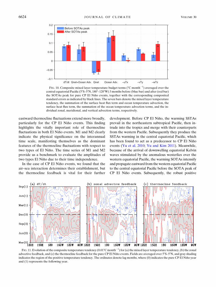
eastward thermocline fluctuations extend more broadly,

particularly for the CP El Niño events. This finding

highlights the vitally important role of thermocline

fluctuations in both El Niño events. M1 and M2 clearly

indicate the physical significance on the interannual

time scale, manifesting themselves as the dominant

features of the thermocline fluctuations with respect to

two types of El Niño. The time series of M1 and M2

provide us a benchmark to evaluate the amplitudes of

two types El Niño due to their time independence.

In the case of CP El Niño events, we found that the

air–sea interaction determines their establishment, but

the thermocline feedback is vital for their further

development. Before CP El Niño, the warming SSTAs

prevail in the northeastern subtropical Pacific, then in-

trude into the tropics and merge with their counterparts

from the western Pacific. Subsequently they produce the

SSTAs warming in the central equatorial Pacific, which

has been found to act as a predecessor to CP El Niñoevents (Yu et al. 2010; Yu and Kim 2011). Meanwhile,

because of the arrival of downwelling equatorial Kelvin

waves stimulated by the anomalous westerlies over the

western equatorial Pacific, the warming SOTAs intensify

andpropagate eastward from thewestern equatorial Pacific

to the central equatorial Pacific before the SOTA peak of

CP El Niño events. Subsequently, the robust positive

FIG. 11. Evolution of the composite temperature tendency (0.018Cmonth21) for (a) themixed layer temperature tendency, (b) the zonal

advective feedback, and (c) the thermocline feedback for the pure CP El Niño events. Fields are averaged over 58S–58N, and gray shading

indicates the region of the positive temperature tendency. The ordinates denote lag months, where (0) indicates the pure CP El Niño year

and (1) represents the following year.

FIG. 10. Composite mixed layer temperature budget terms (8C month21) averaged over the

central equatorial Pacific (58S–58N, 1808–1208W) 3months before (blue bar) and after (red bar)

the SOTAs peak for pure CP El Niño events, together with the corresponding composited

standard errors as indicated by black lines. The seven bars denote the mixed layer temperature

tendency, the summation of the surface heat flux term and ocean temperature advection, the

surface heat flux term, the summation of the ocean temperature advection terms, and the in-

dividual zonal, meridional, and vertical advection terms, respectively.

6624 JOURNAL OF CL IMATE VOLUME 30

SOTAs further expand upward and eastward, resulting in

enhanced SSTAs in the central equatorial Pacific via the

thermocline feedback. With the help of a mixed layer heat

budget analysis, we further demonstrate that the zonal

advective feedback contributes mainly to the development

stage before the SOTA peak of CP El Niño events, while

the thermocline adjustment processes are vital for the pe-

riod after the SOTA peak of CP El Niño events.

It is noted the results might be different because of the

methods. For instance, Ren and Jin (2013) suggested

that thermocline feedback plays a dominant role in the

growth and phase transitions of CP El Niño events,

whereas the zonal advective feedback contributes

mainly to their phase transitions. Wen et al. (2014)

proposed that the enhanced off-equatorial thermocline

plays an important role in the development of El Niñoevents after 1999. Nevertheless, all of the findings sug-

gest that equatorial Pacific thermocline dynamics play a

dominant role during the life cycle of the CP El Niño.Furthermore, the basin-mean equatorial thermocline

depth exhibits a notable decadal variability in the Pacific

(Fig. 1b) due to the equatorial Pacific surface wind stress

forcing (Li and Ren 2012; Kosaka and Xie 2013).

Therefore, more attention should be paid to its impor-

tance in the two types of El Niño cycles.

Our results are primarily from statistical analyses; the

dynamics of equatorial thermocline fluctuations need a

modeling study. In addition, herewemainly discussedM1

and M2; the physical meaning of the higher modes in the

equatorial thermocline will be explored in future studies.

Acknowledgments. The authors gratefully acknowl-

edged the valuable comments and suggestions given by

the editor (Dr. Tim Li) and the anonymous reviewers,

and also thank Dr. Boqi Liu for his constructive sugges-

tions. This work is jointly supported by the Funds for

Creative Research Groups of China (Grant 41521005),

the Special Fund for Public Welfare Industry

(GYHY201506013), the Strategic Priority Research

Program of the Chinese Academy of Sciences (Grant

XDA11010301), and the National Natural Science

Foundation of China (Grants 41406033, 41475057,

41376024, 41676013) and the CAS/SAFEA International

Partnership Program for Creative Research Teams.

APPENDIX

Mode Function Decomposition Method

The lowest-order mode (or mode 0) of the equatorial

thermocline is a constant, f0 [ 1, representing the mean

depth of the equatorial thermocline. Therefore, the

thermocline depth deviation from this basin-mean depth

can be decomposed into a series of mode functions. The

mode functions are defined over the domain [21, 11],

and they are orthogonal to each other, as a fundamental

requirement. These modes start from a value of 21 at

the left edge of the domain (i.e., x 5 21) and consist of

line segments that vary within the range [21,11]. Mode

n has n zero-crossings. As a result, the first mode is a

straight line from (21, 21) to (11, 11), and all other

modes are composed of the straight line segments

between 21 and 11, as shown in Fig. A1. The tradition

in oceanography is to label depth as a positive value and

define the downward direction as positive. This is op-

posite to the common practice in meteorology; however,

in presenting the anomalous signals associated with the

thermocline depth, this method can present the signals

in a simple and accurate way.

Thesemode functions are further spatially normalized

to a series of functions f(x) satisfying the following

unification constraints:

ð121

fi(x)f

j(x) dx5 d

ij(i, j$ 1), (A1)

where the subscripts i and j are the mode numbers, and

d is the Kronecker delta function. Regarding the tem-

poral evolution of the decomposed modes, the main

equatorial thermocline depth anomalies D(x, t) aver-

aged between 58S and 58N, defined over the non-

dimensional domain x5 [21,11], can be projected onto

thesemode function series for any given time t as follows:

D(x, t)5 �‘

i51

ai(t)f

i(x); a

i(t)5

ð121

fi(x)D(x, t) dx, (A2)

where ai(t) is the time evolution for each mode i. The

related code and data for the mode function de-

composition method can be obtained online at https://

github.com/xu-kang/MDF.

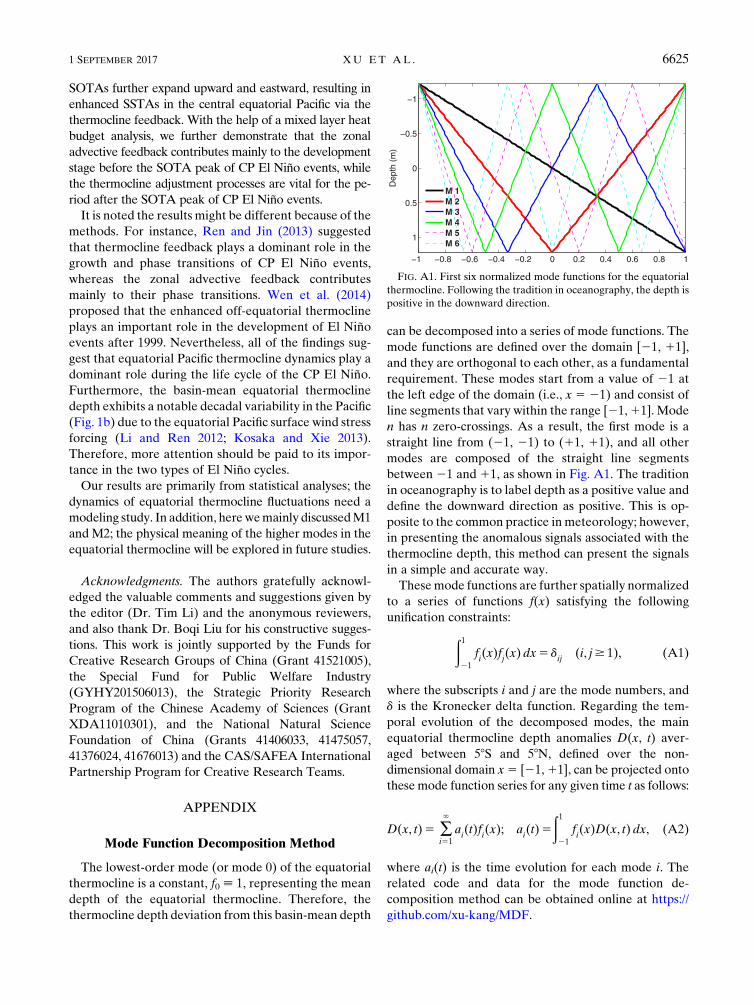
FIG. A1. First six normalized mode functions for the equatorial

thermocline. Following the tradition in oceanography, the depth is

positive in the downward direction.

1 SEPTEMBER 2017 XU ET AL . 6625

Figure A1 presents the visual image of the normalized

structures of the first six mode functions. The mode

functions are orthogonal to each other and have the

same amplitude of 1.22; thus, in terms of thermocline

depth variability, the amplitude of the contribution from

each mode is 1.22ai(t). As seen in Fig. A1, the spatial

structure of the first mode (M1, depicted by a solid black

line), clearly shows a basinwide east–west-tilted ther-

mocline, with shoaling in the west and deepening in the

east, which depicts the basic feature of classical EP El

Niño events (Fig. A1). However, the second mode (M2,

marked by the V-shaped red curve) has a deeper ther-

mocline positioned in the central Pacific Ocean basin

and a shallower thermocline on both side boundaries,

representing the characteristic of CP El Niño events

(Fig. A1). Therefore, this mode function decomposition

method may provide a direct physical interpretation of

the equatorial thermocline using only a few modes, and

the first two leading modes have better capabilities in

capturing and distinguishing the characteristics of the

two types of El Niño events.

REFERENCES

Ashok, K., and T. Yamagata, 2009: Climate change: The El Niñowith a difference. Nature, 461, 481–484, doi:10.1038/461481a.

——, S. K. Behera, S. A. Rao, H.Weng, and T. Yamagata, 2007: El

Niño Modoki and its possible teleconnection. J. Geophys.

Res., 112, C11007, doi:10.1029/2006JC003798.

Behringer, D.W., andY. Xue, 2004: Evaluation of the global ocean

data assimilation system at NCEP: The Pacific Ocean. Proc.

Eighth Symp. on Integrated Observing and Assimilation Sys-

tems for Atmosphere, Oceans, and Land Surface, Seattle, WA,

Amer. Meteor. Soc., 2.3. [Available online at https://ams.

confex.com/ams/pdfpapers/70720.pdf.]

Carton, J. A., B. S. Giese, and S. A. Grodsky, 2005: Sea level rise

and the warming of the oceans in the Simple Ocean Data

Assimilation (SODA) ocean reanalysis. J. Geophys. Res., 110,

C09006, doi:10.1029/2004JC002817.

Chen, L., T. Li, S. K. Behera, and T. Doi, 2016: Distinctive

precursory air–sea signals between regular and super El

Niños. Adv. Atmos. Sci., 33, 996–1004, doi:10.1007/

s00376-016-5250-8.

Chung, P., and T. Li, 2013: Interdecadal relationship between the

mean state and El Niño types. J. Climate, 26, 361–379,

doi:10.1175/JCLI-D-12-00106.1.

Compo, G. P., and Coauthors, 2011: The Twentieth Century Re-

analysis Project. Quart. J. Roy. Meteor. Soc., 137, 1–28,

doi:10.1002/qj.776.

Gu, D., and S. G. H. Philander, 1997: Interdecadal climate fluctu-

ations that depend on exchanges between the tropics and

extratropics. Science, 275, 805–807, doi:10.1126/science.275.

5301.805.

Jin, F.-F., 1997: An equatorial ocean recharge paradigm for ENSO.

Part I: Conceptual model. J. Atmos. Sci., 54, 811–829,

doi:10.1175/1520-0469(1997)054,0811:AEORPF.2.0.CO;2.

Kang, I.-S., and J.-S. Kug, 2002: El Niño and La Niña sea surface

temperature anomalies: Asymmetry characteristics associated

with their wind stress anomalies. J. Geophys. Res., 107, 4372,

doi:10.1029/2001JD000393.

Kao, H., and J. Yu, 2009: Contrasting eastern-Pacific and central-

Pacific types of ENSO. J. Climate, 22, 615–632, doi:10.1175/

2008JCLI2309.1.

Kessler, W. S., 1990: Observations of long Rossby waves in the

northern tropical Pacific. J. Geophys. Res., 95, 5183–5217,

doi:10.1029/JC095iC04p05183.

Kim, W., S. Yeh, J. Kim, J. Kug, and M. Kwon, 2011: The unique

2009–2010 El Niño event: A fast phase transition of warm pool

El Niño to La Niña. Geophys. Res. Lett., 38, L15809,

doi:10.1029/2011GL048521.

Kosaka, Y., and S.-P. Xie, 2013: Recent global-warming hiatus tied

to equatorial Pacific surface cooling. Nature, 501, 403–407,

doi:10.1038/nature12534.

Kug, J.-S., F.-F. Jin, and S.-I. An, 2009: Two types of El Niñoevents: Cold tongue El Niño and warm pool El Niño.J. Climate, 22, 1499–1515, doi:10.1175/2008JCLI2624.1.

——, J. Choi, S. An, F. Jin, and A. T.Wittenberg, 2010:Warm pool

and cold tongue El Niño events as simulated by the GFDL 2.1

coupled GCM. J. Climate, 23, 1226–1239, doi:10.1175/

2009JCLI3293.1.

Larkin, N. K., and D. E. Harrison, 2005: On the definition of El

Niño and associated seasonal average U.S. weather anomalies.

Geophys. Res. Lett., 32, L13705, doi:10.1029/2005GL022738.

Lee, T., and M. J. McPhaden, 2010: Increasing intensity of El Niñoin the central-equatorial Pacific. Geophys. Res. Lett., 37,

L14603, doi:10.1029/2010GL044007.

Li, G., and B. Ren, 2012: Evidence for strengthening of the tropical

Pacific Ocean surface wind speed during 1979–2001. Theor.

Appl. Climatol., 107, 59–72, doi:10.1007/s00704-011-0463-3.Li, T., T. F. Hogan, and C. Chang, 2000: Dynamic and thermody-

namic regulation of ocean warming. J. Atmos. Sci., 57, 3353–

3365, doi:10.1175/1520-0469(2000)057,3353:DATROO.2.0.

CO;2.

——, Y. Zhang, E. Lu, and D. Wang, 2002: Relative role of dy-

namic and thermodynamic processes in the development of

the Indian Ocean dipole: AnOGCM diagnosis.Geophys. Res.

Lett., 29, 2110, doi:10.1029/2002GL015789.

Li, X., C. Li, J. Ling, and Y. Tan, 2015: The relationship between

contiguous El Niño and La Niña revealed by self-organizing

maps. J. Climate, 28, 8118–8134, doi:10.1175/

JCLI-D-15-0123.1.

McPhaden, M. J., S. E. Zebiak, and M. H. Glantz, 2006: ENSO as

an integrating concept in Earth science. Science, 314, 1740–

1745, doi:10.1126/science.1132588.

Meinen, C. S., and M. J. McPhaden, 2000: Observations of

warm water volume changes in the equatorial Pacific

and their relationship to El Niño and La Niña. J. Climate,

13, 3551–3559, doi:10.1175/1520-0442(2000)013,3551:

OOWWVC.2.0.CO;2.

North, G. R., T. L. Bell, R. F. Cahalan, and F. J. Moeng, 1982:

Sampling errors in the estimation of empirical orthogonal

functions. Mon. Wea. Rev., 110, 699–706, doi:10.1175/

1520-0493(1982)110,0699:SEITEO.2.0.CO;2.

Pedlosky, J., 1987: An inertial theory of the equatorial un-

dercurrent. J. Phys. Oceanogr., 17, 1978–1985, doi:10.1175/

1520-0485(1987)017,1978:AITOTE.2.0.CO;2.

Rayner, N. A., D. E. Parker, E. B. Horton, C. K. Folland, L. V.

Alexander, D. P. Rowell, E. C. Kent, and A. Kaplan, 2003:

Global analyses of sea surface temperature, sea ice, and night

marine air temperature since the late nineteenth century.

J. Geophys. Res., 108, 4407, doi:10.1029/2002JD002670.

6626 JOURNAL OF CL IMATE VOLUME 30

Ren, H., and F. Jin, 2011: Niño indices for two types of ENSO.

Geophys. Res. Lett., 38, L04704, doi:10.1029/2010GL046031.

——, and ——, 2013: Recharge oscillator mechanisms in two

types of ENSO. J. Climate, 26, 6506–6523, doi:10.1175/

JCLI-D-12-00601.1.

Su, J., T. Li, and R. Zhang, 2014: The initiation and developing

mechanisms of central Pacific El Niños. J. Climate, 27, 4473–

4485, doi:10.1175/JCLI-D-13-00640.1.

Trenberth, K. E., and D. P. Stepaniak, 2001: Indices of El

Niño evolution. J. Climate, 14, 1697–1701, doi:10.1175/

1520-0442(2001)014,1697:LIOENO.2.0.CO;2.

Wang, C., and X. Wang, 2013: Classifying El Niño Modoki I and II

by different impacts on rainfall in southern China and

typhoon tracks. J. Climate, 26, 1322–1338, doi:10.1175/

JCLI-D-12-00107.1.

Wang, L., T. Li, and T. Zhou, 2012: Intraseasonal SST variability

and air–sea interaction over the Kuroshio Extension region

during boreal summer. J. Climate, 25, 1619–1634, doi:10.1175/

JCLI-D-11-00109.1.

Wang, X., and C.Wang, 2014: Different impacts of various El Niñoevents on the Indian Ocean dipole. Climate Dyn., 42, 991–

1005, doi:10.1007/s00382-013-1711-2.

Wen, C., A. Kumar, Y. Xue, andM. J. McPhaden, 2014: Changes in

tropical Pacific thermocline depth and their relationship to

ENSO after 1999. J. Climate, 27, 7230–7249, doi:10.1175/

JCLI-D-13-00518.1.

Weng, H., K. Ashok, S. K. Behera, S. A. Rao, and T. Yamagata,

2007: Impacts of recent El NiñoModoki on dry/wet conditions

in the Pacific rim during boreal summer. Climate Dyn., 29,

113–129, doi:10.1007/s00382-007-0234-0.

Wyrtki, K., 1989: Some thoughts about the west Pacific warm pool.

Proc. West Pacific Int. Meeting and Workshop on TOGA

COARE, Nouméa, New Caledonia, Office de la recherche

scientifique et technique outre-mer (ORSTOM), 99–109.

Xiang, B., B. Wang, and T. Li, 2013: A new paradigm for the

predominance of standing central Pacific warming after

the late 1990s. Climate Dyn., 41, 327–340, doi:10.1007/

s00382-012-1427-8.

Xie, S.-P., and S. G. H. Philander, 1994: A coupled ocean–

atmosphere model of relevance to the ITCZ in the eastern

Pacific. Tellus, 46A, 340–350, doi:10.3402/tellusa.v46i4.15484.

Xu, K., C. Zhu, and J. He, 2012: Linkage between the dominant

modes in Pacific subsurface ocean temperature and the two

type ENSO events. Chin. Sci. Bull., 57, 3491–3496,

doi:10.1007/s11434-012-5173-4.

——, ——, and——, 2013: Two types of El Niño-related Southern

Oscillation and their different impacts on global land pre-

cipitation. Adv. Atmos. Sci., 30, 1743–1757.——, J. Su, and C. Zhu, 2014: The natural oscillation of two types of

ENSO events based on analyses of CMIP5model control runs.

Adv. Atmos. Sci., 31, 801–813, doi:10.1007/s00376-013-3153-5.

——, C.-Y. Tam, C. Zhu, B. Liu, and W. Wang, 2017: CMIP5

projections of two types of El Niño and their related tropical

precipitation in the twenty-first century. J. Climate, 30, 849–

864, doi:10.1175/JCLI-D-16-0413.1.

Yeh, S., J. Kug, B. Dewitte, M. Kwon, B. P. Kirtman, and F. Jin,

2009: El Niño in a changing climate. Nature, 461, 511–514,

doi:10.1038/nature08316.

Yu, J.-Y., and H.-Y. Kao, 2007: Decadal changes of ENSO per-

sistence barrier in SST and ocean heat content indices: 1958–

2001. J. Geophys. Res., 112, D13106, doi:10.1029/

2006JD007654.

——, and S. T. Kim, 2011: Relationships between extratropical sea

level pressure variations and the central Pacific and eastern

Pacific types of ENSO. J. Climate, 24, 708–720, doi:10.1175/

2010JCLI3688.1.

——, H.-Y. Kao, and T. Lee, 2010: Subtropics-related interannual

sea surface temperature variability in the central equatorial

Pacific. J. Climate, 23, 2869–2884, doi:10.1175/

2010JCLI3171.1.

——, ——, ——, and S. T. Kim, 2011: Subsurface ocean tempera-

ture indices for central-Pacific and eastern-Pacific types of El

Niño and La Niña events. Theor. Appl. Climatol., 103, 337–

344, doi:10.1007/s00704-010-0307-6.

——, Y. Zou, S. T. Kim, and T. Lee, 2012: The changing impact of

El Niño on US winter temperatures. Geophys. Res. Lett., 39,

L15702, doi:10.1029/2012GL052483.

Zhang,W., F. Jin, and A. Turner, 2014: Increasing autumn drought

over southern China associated with ENSO regime shift. Ge-

ophys. Res. Lett., 41, 4020–4026, doi:10.1002/2014GL060130.

——, Y. Wang, F. Jin, M. F. Stuecker, and A. G. Turner, 2015:

Impact of different El Niño types on the El Niño/IOD re-

lationship. Geophys. Res. Lett., 42, 8570–8576, doi:10.1002/

2015GL065703.

1 SEPTEMBER 2017 XU ET AL . 6627