The Euler–Poincaré Equations and Semidirect Products with Applications to Continuum Theories
81
Advances in Mathematics 137, 181 (1998) The EulerPoincare Equations and Semidirect Products with Applications to Continuum Theories Darryl D. Holm Theoretical Division and Center for Nonlinear Studies, Los Alamos National Laboratory, MS B284, Los Alamos, New Mexico 87545 E-mail: dholmlanl.gov Jerrold E. Marsden* Control and Dynamical Systems, California Institute of Technology, 107-81, Pasadena, California 91125 E-mail: marsdencds.caltech.edu and Tudor S. Ratiu - Department of Mathematics, University of California, Santa Cruz, California 95064 E-mail: ratiumath.ucsc.edu Received November 17, 1997; accepted January 3, 1998 We study EulerPoincare systems (i.e., the Lagrangian analogue of LiePoisson Hamiltonian systems) defined on semidirect product Lie algebras. We first give a derivation of the EulerPoincare equations for a parameter dependent Lagrangian by using a variational principle of Lagrange d'Alembert type. Then we derive an abstract KelvinNoether theorem for these equations. We also explore their rela- tion with the theory of LiePoisson Hamiltonian systems defined on the dual of a semidirect product Lie algebra. The Legendre transformation in such cases is often not invertible; thus, it does not produce a corresponding EulerPoincare system on that Lie algebra. We avoid this potential difficulty by developing the theory of EulerPoincare systems entirely within the Lagrangian framework. We apply the general theory to a number of known examples, including the heavy top, ideal com- pressible fluids and MHD. We also use this framework to derive higher dimensional CamassaHolm equations, which have many potentially interesting analytical properties. These equations are EulerPoincare equations for geodesics on diffeo- morphism groups (in the sense of the Arnold program) but where the metric is H 1 rather than L 2 . 1998 Academic Press Article No. AI981721 1 0001-870898 25.00 Copyright 1998 by Academic Press All rights of reproduction in any form reserved. * Research partially by NSF grant DMS 96-33161. - Research partially supported by NSF Grant DMS-9503273 and DOE contract DE-FG03- 95ER25245-A000.
Transcript of The Euler–Poincaré Equations and Semidirect Products with Applications to Continuum Theories

File: DISTL2 172101 . By:CV . Date:11:06:98 . Time:10:43 LOP8M. V8.B. Page 01:01Codes: 4160 Signs: 2153 . Length: 50 pic 3 pts, 212 mm
Advances in Mathematics � AI1721
Advances in Mathematics 137, 1�81 (1998)
The Euler�Poincare� Equations and Semidirect Productswith Applications to Continuum Theories
Darryl D. Holm
Theoretical Division and Center for Nonlinear Studies, Los Alamos National Laboratory,MS B284, Los Alamos, New Mexico 87545
E-mail: dholm�lanl.gov
Jerrold E. Marsden*
Control and Dynamical Systems, California Institute of Technology,107-81, Pasadena, California 91125
E-mail: marsden�cds.caltech.edu
and
Tudor S. Ratiu-
Department of Mathematics, University of California, Santa Cruz, California 95064
E-mail: ratiu�math.ucsc.edu
Received November 17, 1997; accepted January 3, 1998
We study Euler�Poincare� systems (i.e., the Lagrangian analogue of Lie�PoissonHamiltonian systems) defined on semidirect product Lie algebras. We first give aderivation of the Euler�Poincare� equations for a parameter dependent Lagrangianby using a variational principle of Lagrange d'Alembert type. Then we derive anabstract Kelvin�Noether theorem for these equations. We also explore their rela-tion with the theory of Lie�Poisson Hamiltonian systems defined on the dual of asemidirect product Lie algebra. The Legendre transformation in such cases is oftennot invertible; thus, it does not produce a corresponding Euler�Poincare� system onthat Lie algebra. We avoid this potential difficulty by developing the theory ofEuler�Poincare� systems entirely within the Lagrangian framework. We apply thegeneral theory to a number of known examples, including the heavy top, ideal com-pressible fluids and MHD. We also use this framework to derive higher dimensionalCamassa�Holm equations, which have many potentially interesting analyticalproperties. These equations are Euler�Poincare� equations for geodesics on diffeo-morphism groups (in the sense of the Arnold program) but where the metric is H1
rather than L2. � 1998 Academic Press
Article No. AI981721
10001-8708�98 �25.00
Copyright � 1998 by Academic PressAll rights of reproduction in any form reserved.
* Research partially by NSF grant DMS 96-33161.- Research partially supported by NSF Grant DMS-9503273 and DOE contract DE-FG03-
95ER25245-A000.

File: DISTL2 172102 . By:CV . Date:11:06:98 . Time:10:43 LOP8M. V8.B. Page 01:01Codes: 2807 Signs: 2062 . Length: 45 pic 0 pts, 190 mm
Contents.1. History and Background2. Hamiltonian Semidirect Product Theory3. Lagrangian Semidirect Product Theory4. The Kelvin�Noether Theorem5. The Heavy Top6. The Euler�Poincare� Equations in Continuum Mechanics7. Applications of the Euler�Poincare� Theorem to Continua8. Approximate Model Fluid Equations which Preserve the Euler�Poincare� Structure
Appendix
1. HISTORY AND BACKGROUND
To put our paper in context, we shall pick up the thread of the historyof mechanics in the later part of the 1800s. By that time, through the workof many people, including Euler, Lagrange, Hamilton, Jacobi, and Routh,it was well understood that the equations of mechanics are expressible ineither Hamiltonian or Lagrangian form.
The Lagrangian formulation of mechanics can be based on the varia-tional principles behind Newton's fundamental laws of force balanceF=ma. One chooses a configuration space Q (a manifold, assumed to beof finite dimension n to start the discussion) with coordinates denoted qi,i=1, ..., n, that describe the configuration of the system under study. Onethen forms the velocity phase space TQ (the tangent bundle of Q).Coordinates on TQ are denoted (q1, ..., qn, q* 1, ..., q* n), and the Lagrangian isregarded as a function L: TQ � R. In coordinates, one writes L(qi, q* i, t),which is shorthand notation for L(q1, ..., qn, q* 1, ..., q* n, t). Usually, L is thekinetic minus the potential energy of the system and one takes q* i=dqi�dtto be the system velocity. The variational principle of Hamilton states thatthe variation of the action is stationary at a solution:
$S=$ |b
aL(qi, q* i, t) dt=0. (1.1)
In this principle, one chooses curves qi (t) joining two fixed points in Qover a fixed time interval [a, b], and calculates the action S, which is thetime integral of the Lagrangian, regarded as a function of this curve.Hamilton's principle states that the action S has a critical point at asolution in the space of curves. As is well known, Hamilton's principle isequivalent to the Euler�Lagrange equations:
ddt
�L�q* i&
�L�qi=0, i=1, ..., n. (1.2)
2 HOLM, MARSDEN, AND RATIU

File: DISTL2 172103 . By:CV . Date:11:06:98 . Time:10:43 LOP8M. V8.B. Page 01:01Codes: 2460 Signs: 1571 . Length: 45 pic 0 pts, 190 mm
If the system is subjected to external forces, these are to be added to theright hand side of the Euler�Lagrange equations. For the case in which Lcomprises kinetic minus potential energy, the Euler�Lagrange equationsreduce to a geometric form of Newton's second law. For Lagrangians thatare purely kinetic energy, it was already known in Poincare� 's time that thecorresponding solutions of the Euler�Lagrange equations are geodesics.(This fact was certainly known to Jacobi by 1840, for example.)
To pass to the Hamiltonian formalism, one introduces the conjugatemomenta
pi=�L�q* i , i=1, ..., n, (1.3)
and makes the change of variables (qi, q* i) [ (qi, pi), by a Legendre trans-formation. The Lagrangian is called regular when this change of variablesis invertible. The Legendre transformation introduces the Hamiltonian
H(qi, pi , t)= :n
j=1
pj q* j=L(qi, q* i, t). (1.4)
One shows that the Euler�Lagrange equations are equivalent to Hamilton'sequations:
dqi
dt=
�H�pi
,dpi
dt=&
�H�qi , (1.5)
where i=1, ..., n. There are analogous Hamiltonian partial differentialequations for field theories such as Maxwell's equations and the equationsof fluid and solid mechanics.
Hamilton's equations can be recast in Poisson bracket form as
F4 =[F, H], (1.6)
where the canonical Poisson brackets are given by
[F, G]= :n
i=1\�F
�qi
�G�pi
&�F�pi
�G�qi+ . (1.7)
Associated to any configuration space Q is a phase space T*Q called thecotangent bundle of Q, which has coordinates (q1, ..., qn, p1 , ..., pn). On thisspace, the canonical Poisson bracket is intrinsically defined in the sense
3EULER�POINCARE� AND SEMIDIRECT PRODUCTS
File: DISTL2 172104 . By:CV . Date:11:06:98 . Time:10:43 LOP8M. V8.B. Page 01:01Codes: 3167 Signs: 2675 . Length: 45 pic 0 pts, 190 mm
that the value of [F, G] is independent of the choice of coordinates.Because the Poisson bracket satisfies [F, G]=&[G, F] and in particular[H, H]=0, we see that H4 =0; that is, energy is conserved along solutionsof Hamilton's equations. This is the most elementary of many deep andbeautiful conservation properties of mechanical systems.
Poincare� and the Euler equations. Poincare� played an enormous role inthe topics treated in the present paper. We mention a few of Poincare� 'scontributions that are relevant here. First is his work on the gravitatingfluid problem, continuing the line of investigation begun by MacLaurin,Jacobi, and Riemann. Some solutions of this problem still bear his nametoday. This work is summarized in Chandrasekhar [1967, 1977] (seePoincare� [1885, 1890, 1892, 1901a] for the original treatments). This back-ground led to his famous paper, Poincare� [1901b], in which he laid outthe basic equations of Euler type, including the rigid body, heavy top andfluids as special cases. Abstractly, these equations are determined once oneis given a Lagrangian on a Lie algebra. We shall make some additionalhistorical comments on this situation below, after we present a few moremechanical preliminaries. It is because of the paper Poincare� [1901b] thatthe name Euler�Poincare� equations is now used for these equations.
To state the Euler�Poincare� equations, let g be a given Lie algebra andlet l : g � R be a given function (a Lagrangian), let ! be a point in g andlet f # g* be given forces (whose nature we shall explicate later). Then theevolution of the variable ! is determined by the Euler�Poincare� equations.Namely,
ddt
$l$!
=ad!*$l$!
+ f.
The notation is as follows: �l��! # g* (the dual vector space) is thederivative of l with respect to !; we use partial derivative notation becausel is a function of the vector xi and because shortly l will be a function ofother variables as well. The map ad! : g � g is the linear map ' [ [!, '],where [!, '] denotes the Lie bracket of ! and ', and where ad!* : g* � g*is its dual (transpose) as a linear map. In the case that f =0, we will callthese equations the basic Euler�Poincare� equations.
These equations are valid for either finite or infinite dimensional Liealgebras. For fluids, Poincare� was aware that one needs to use infinitedimensional Lie algebras, as is clear in his paper Poincare� [1910]. He wasaware that one has to be careful with the signs in the equations; forexample, for rigid body dynamics one uses the equations as they stand, butfor fluids, one needs to be careful about the conventions for the Lie algebraoperation ad! ; cf. Chetayev [1941].
4 HOLM, MARSDEN, AND RATIU

File: DISTL2 172105 . By:CV . Date:11:06:98 . Time:10:43 LOP8M. V8.B. Page 01:01Codes: 2903 Signs: 2217 . Length: 45 pic 0 pts, 190 mm
To state the equations in the finite dimensional case in coordinates, onemust choose a basis e1 , ..., er of g (so dim g=r). Define, as usual, thestructure constants C d
ab of the Lie algebra by
[ea , eb]= :r
d=1
C dabed , (1.8)
where a, b run from 1 to r. If ! # g, its components relative to this basis aredenoted !a. If e1, ..., en, is the corresponding dual basis, then the com-ponents of the differential of the Lagrangian l are the partial derivatives�l��!a. The Euler�Poincare� equations in this basis are
ddt
�l�!b= :
r
a, d=1
C dab
�l�!d !a+ fb . (1.9)
For example, consider the Lie algebra R3 with the usual vector crossproduct. (Of course, this is the Lie algebra of the proper rotation groupin R3.) For l : R3 � R, the Euler�Poincare� equations become
ddt
�l�0
_0+f,
which generalize the Euler equations for rigid body motion.These equations were written down for a certain class of Lagrangians l
by Lagrange [1788, Volume 2, Eq. A, p. 212], while it was Poincare�[1901b] who generalized them (without reference to the ungeometricLagrange!) to an arbitrary Lie algebra. However, it was Lagrange who wasgrappeling with the derivation and deeper understanding of the nature ofthese equations. While Poincare� may have understood how to derive themfrom other principles, he did not reveal this.
Of course, there was a lot of mechanics going on in the decades leadingup to Poincare� 's work and we shall comment on some of it below.However, it is a curious historical fact that the Euler�Poincare� equationswere not pursued extensively until quite recently. While many authorsmentioned these equations and even tried to understand them more deeply(see, e.g., Hamel [1904, 1949] and Chetayev [1941]), it was not until theArnold school that this understanding was at least partly achieved (seeArnold [1966a, c] and Arnold [1988]) and was used for diagnosing hydro-dynamical stability (e.g., Arnold [1966b]).
It was already clear in the last century that certain mechanical systemsresist the usual canonical formalism, either Hamiltonian or Lagrangian,outlined in the first paragraph. The rigid body provides an elementaryexample of this. In another example, to obtain a Hamiltonian description
5EULER�POINCARE� AND SEMIDIRECT PRODUCTS

File: DISTL2 172106 . By:CV . Date:11:06:98 . Time:10:43 LOP8M. V8.B. Page 01:01Codes: 3008 Signs: 1971 . Length: 45 pic 0 pts, 190 mm
for ideal fluids, Clebsch [1857, 1859] found it necessary to introducecertain nonphysical potentials.1
More About the Rigid Body. In the absence of external forces, the rigidbody equations are usually written as follows:
I104 1=(I2&I3) 0203 ,
I204 2=(I3&I1) 0301 , (1.10)
I304 3=(I1&I2) 0102 ,
where 0=(01 , 02 , 03) is the body angular velocity vector and I1 , I2 , I3
are the moments of inertia of the rigid body. Are these equations as writtenLagrangian or Hamiltonian in any sense? Since there are an odd numberof equations, they cannot be put in canonical Hamiltonian form.
One answer is to reformulate the equations on TSO(3) on T*SO(3), asis classically done in terms of Euler angles and their velocities or conjugatemomenta, relative to which the equations are in Euler�Lagrange or canoni-cal Hamiltonian form. However, this reformulation answers a differentquestion for a six dimensional system. We are interested in these structuresfor the equations as given above.
The Lagrangian answer is easy: These equations have Euler�Poincare�form on the Lie algebra R3 using the Lagrangian
l(0)= 12 (I1 02
1+I2022+I302
3), (1.11)
which is the (rotational) kinetic energy of the rigid body.One of our main messages is that the Euler�Poincare� equations possess
a natural variational principle. In fact, the Euler rigid body equations areequivalent to the rigid body action principle
$Sred=$ |b
al dt=0, (1.12)
where variations of 0 are restricted to be of the form
$0=74 +0_7, (1.13)
in which 7 is a curve in R3 that vanishes at the endpoints. As before, weregard the reduced action Sred as a function on the space of curves, butonly consider variations of the form described. The equivalence of the rigid
6 HOLM, MARSDEN, AND RATIU
1 For modern accounts of Clebsch potentials and further references, see Holm andKupershmidt [1983], Marsden and Weinstein [1983], Marsden, Ratiu, and Weinstein[1984a, b], Cendra and Marsden [1987], Cendra, Ibort, and Marsden [1987] andGoncharov and Pavlov [1997].

File: DISTL2 172107 . By:CV . Date:11:06:98 . Time:10:43 LOP8M. V8.B. Page 01:01Codes: 2311 Signs: 1325 . Length: 45 pic 0 pts, 190 mm
body equations and the rigid body action principle may be proved in thesame way as one proves that Hamilton's principle is equivalent to theEuler�Lagrange equations: Since l(0)= 1
2 (I0, 0) , and I is symmetric, weobtain
$ |b
al dt=|
b
a(I0, $0) dt
=|b
a(I0, 74 +0_7) dt
=|b
a _�&ddt
I0, 7�+(I0, 0_7)&=|
b
a �&ddt
I0+I0_0, 7� dt,
where we used integration by parts and the endpoint conditions 7(b)=7(a)=0. Since 7 is otherwise arbitrary, (1.12) is equivalent to
&ddt
(I0)+I0_0=0,
which are Euler's equations.Let us explain in concrete terms (that will be abstracted later) how to
derive this variational principle from the standard variational principle ofHamilton.
We regard an element R # SO(3) giving the configuration of the body asa map of a reference configuration B/R3 to the current configurationR(B); the map R takes a reference or label point X # B to a current pointx=R(X) # R(B). When the rigid body is in motion, the matrix R is time-dependent and the velocity of a point of the body is x* =R4 X=R4 R&1x.Since R is an orthogonal matrix, R&1R4 and R4 R&1 are skew matrices, andso we can write
x* =R4 R&1x=|_x, (1.14)
which defines the spatial angular velocity vector |. Thus, | is essentiallygiven by right translation of R4 to the identity.
The corresponding body angular velocity is defined by
0=R&1|, (1.15)
7EULER�POINCARE� AND SEMIDIRECT PRODUCTS

File: DISTL2 172108 . By:CV . Date:11:06:98 . Time:10:43 LOP8M. V8.B. Page 01:01Codes: 2549 Signs: 1474 . Length: 45 pic 0 pts, 190 mm
so that 0 is the angular velocity relative to a body fixed frame. Notice that
R&1R4 X=R&1R4 R&1x=R&1(|_x)
=R&1|_R&1x=0_X, (1.16)
so that 0 is given by left translation of R4 to the identity. The kinetic energyis obtained by summing up m |x* |2�2 (where | v | denotes the Euclideannorm) over the body:
K= 12 |
B
\(x) |R4 X|2 d 3X, (1.17)
in which \ is a given mass density in the reference configuration. Since
|R4 X|=||_x|=|R&1(|_x)|=|0_X|,
K is a quadratic function of 0. Writing
K= 12 0TI0 (1.18)
defines the moment of inertia tensor I, which, provided the body does notdegenerate to a line, is a positive-definite (3_3) matrix, or better, a quad-ratic form. This quadratic form can be diagonalized by a change of basis;thereby defining the principal axes and moments of inertia. In this basis, wewrite I=diag(I1 , I2 , I3). The function K is taken to be the Lagrangian ofthe system on TSO(3) (and by means of the Legendre transformation weobtain the corresponding Hamiltonian description on T*SO(3)). Noticethat K in equation (1.17) is left (not right) invariant on TSO(3). It followsthat the corresponding Hamiltonian is also left invariant.
In the Lagrangian framework, the relation between motion in R spaceand motion in body angular velocity (or 0) space is as follows: The curveR(t) # SO(3) satisfies the Euler�Lagrange equations for
L(R, R4 )= 12 |
B
\(X) |R4 X|2 d 3X, (1.19)
if and only if 0(t) defined by R&1R4 v=0_v for all v # R3 satisfies Euler'sequations
I04 =(I0)_0. (1.20)
8 HOLM, MARSDEN, AND RATIU

File: DISTL2 172109 . By:CV . Date:11:06:98 . Time:10:43 LOP8M. V8.B. Page 01:01Codes: 2386 Signs: 923 . Length: 45 pic 0 pts, 190 mm
An instructive proof of this relation involves understanding how toreduce variational principles using their symmetry groups. By Hamilton'sprinciple, R(t) satisfies the Euler�Lagrange equations, if and only if
$ | L dt=0.
Let l(0)= 12 (I0) } 0, so that l(0)=L(R, R4 ) if R and 0 are related as
above. To see how we should transform Hamilton's principle, define theskew matrix 0� by 0� v=0_v for any v # R3, and differentiate the relationR&1R4 =0� with respect to R to get
&R&1($R) R&1R4 +R&1($R4 )=$0@. (1.21)
Let the skew matrix 7� be defined by
7� =R&1 $R, (1.22)
and define the vector 7 by
7� v=7_v. (1.23)
Note that
7�4 =&R&1R4 R&1 $R+R&1 $R4 ,
so
R&1 $R4 =7�4 +R&1R4 7� . (1.24)
Substituting (1.24) and (1.22) into (1.21) gives
&7� 0� +7�4 +0� 7� =$0@,
that is,
$0@=7�4 +[0� , 7� ]. (1.25)
The identity [0� , 7� ]=(0_7) � holds by Jacobi's identity for the crossproduct and so
$0=74 +0_7. (1.26)
These calculations prove the following:
9EULER�POINCARE� AND SEMIDIRECT PRODUCTS

File: DISTL2 172110 . By:CV . Date:11:06:98 . Time:10:43 LOP8M. V8.B. Page 01:01Codes: 2436 Signs: 999 . Length: 45 pic 0 pts, 190 mm
Theorem 1.1. Hamilton's variational principle
$S=$ |b
aL dt=0 (1.27)
on TSO(3) is equivalent to the reduced variational principle
$Sred=$ |b
al dt=0 (1.28)
on R3 where the variations $0 are of the form (1.26) with 7(a)=7(b)=0.
Hamiltonian Form. If, instead of variational principles, we concentrateon Poisson brackets and drop the requirement that they be in the canoni-cal form, then there is also a simple and beautiful Hamiltonian structurefor the rigid body equations that is now well know.2 To recall this, intro-duce the angular momenta
6i=Ii0i=�L�0i
, i=1, 2, 3, (1.29)
so that the Euler equations become
64 1=I2&I3
I2 I3
62 63 ,
64 2=I2&I1
I3 I1
63 61 , (1.30)
64 3=I1&I2
I1 I2
61 62 ,
that is,
64 =6_0. (1.31)
Introduce the following rigid body Poisson bracket on functions of the 6$s:
[F, G](6)=&6 } ({6 F_{6 G) (1.32)
and the Hamiltonian
H=12 \
6 21
I1
+6 2
2
I2
+6 2
3
I3 + . (1.33)
One checks that Euler's equations are equivalent to F4 =[F, H].
10 HOLM, MARSDEN, AND RATIU
2 See Marsden and Ratiu [1994] for details, references, and the history of this structure.
File: DISTL2 172111 . By:CV . Date:11:06:98 . Time:10:43 LOP8M. V8.B. Page 01:01Codes: 2691 Signs: 1798 . Length: 45 pic 0 pts, 190 mm
The rigid body variational principle and the rigid body Poisson bracketare special cases of general constructions associated to any Lie algebra g.Since we have already described the general Euler�Poincare� constructionon g, we turn next to the Hamiltonian counterpart on the dual space.
The Lie�Poisson Equations. Let F, G be real valued functions on thedual space g*. Denoting elements of g* by +, let the functional derivativeof F at + be the unique element $F�$+ of g defined by
lim= � 0
1=
[F(++=$+)&F(+)]=�$+,$F$+�, (1.34)
for all $+ # g*, where ( , ) denotes the pairing between g* and g. Definethe (\) Lie�Poisson brackets by
[F, G]\ (+)=\�+, _$F$+
,$G$+&�. (1.35)
Using the coordinate notation introduced above, the (\) Lie�Poissonbrackets become
[F, G]\ (+)=\ :r
a, b, d=1
Cdab +d
�F�+a
�G�+b
, (1.36)
where +=�rd=1 +ded.
The Lie�Poisson equations, determined by F4 =[F, H] read
+* a=\ :r
b, d=1
C dab+d
�H�+b
,
or intrinsically,
+* =�ad*�H��+ +. (1.37)
This setting of mechanics is a special case of the general theory of systemson Poisson manifolds, for which there is now an extensive theoreticaldevelopment. (See Guillemin and Sternberg [1984] and Marsden andRatiu [1994] for a start on this literature.) There is an especially importantfeature of the rigid body bracket that carries over to general Lie algebras,namely, Lie�Poisson brackets arise from canonical brackets on the cotangentbundle (phase space) T*G associated with a Lie group G which has g as itsassociated Lie algebra.
For a rigid body which is free to rotate about its center of mass, G is the(proper) rotation group SO(3). The choice of T*G as the primitive phasespace is made according to the classical procedures of mechanics describedearlier. For the description using Lagrangian mechanics, one forms the
11EULER�POINCARE� AND SEMIDIRECT PRODUCTS

File: DISTL2 172112 . By:CV . Date:11:06:98 . Time:10:43 LOP8M. V8.B. Page 01:01Codes: 3252 Signs: 2833 . Length: 45 pic 0 pts, 190 mm
velocity-phase space TSO(3). The Hamiltonian description on T*G is thenobtained by the Legendre transformation.
The passage from T*G to the space of 6's (body angular momentumspace) is determined by left translation on the group. This mapping is anexample of a momentum map; that is, a mapping whose components are the``Noether quantities'' associated with a symmetry group. The map fromT*G to g* being a Poisson (canonical) map is a general fact about momen-tum maps. The Hamiltonian point of view of all this is again a welldeveloped subject.
Geodesic Motion. As emphasized by Arnold [1966a], in many interest-ing cases, the Euler�Poincare� equations on a Lie algebra g correspond togeodesic motion on the corresponding group G. We shall explain the rela-tionship between the equations on g and on G shortly, in Theorem 1.2.Similarly, on the Hamiltonian side, the preceding paragraphs explained therelation between the Hamiltonian equations on T*G and the Lie�Poissonequations on g*. However, the issue of geodesic motion is simple: if theLagrangian or Hamiltonian on g or g* is purely quadratic, then the corre-sponding motion on the group is geodesic motion.
More History. The Lie�Poisson bracket was discovered by Sophus Lie(Lie [1890], Vol. II, p. 237). However, Lie's bracket and his related workwas not given much attention until the work of Kirillov, Kostant, andSouriau (and others) revived it in the mid-1960s. Meanwhile, it was noticedby Pauli and Martin around 1950 that the rigid body equations are inHamiltonian form using the rigid body bracket, but they were apparentlyunaware of the underlying Lie theory. It would seem that while Poincare�was aware of Lie theory, in his work on the Euler equations he wasunaware of Lie's work on Lie�Poisson structures. He also seems not tohave been aware of the variational structure of the Euler equations.
The Heavy Top. Another system important to Poincare� and also for usin this paper is the heavy top; that is, a rigid body with a fixed point in agravitational field. For the Lie�Poisson description, the underlying Liealgebra, surprisingly, consists of the algebra of infinitesimal Euclideanmotions in R3. These do not arise as actual Euclidean motions of the bodysince the body has a fixed point! As we shall see, there is a close parallelwith the Poisson structure for compressible fluids.
The basic phase space we start with is again T*SO(3). In this space, theequations are in canonical Hamiltonian form. Gravity breaks the symmetryand the system is no longer SO(3) invariant, so it cannot be writtenentirely in terms of the body angular momentum 6. One also needs tokeep track of 1, the ``direction of gravity'' as seen from the body (1=R&1kwhere the unit vector k points upward and R is the element of SO(3)
12 HOLM, MARSDEN, AND RATIU

File: DISTL2 172113 . By:CV . Date:11:06:98 . Time:10:43 LOP8M. V8.B. Page 01:01Codes: 2264 Signs: 982 . Length: 45 pic 0 pts, 190 mm
describing the current configuration of the body). The equations of motionare
64 1=I2&I3
I2 I3
62 63+Mgl(1 2/3&1 3/2),
64 2=I3&I1
I3 I2
63 61+Mgl(1 3/1&1 1/3), (1.38)
64 3=I1&I2
I1 I2
61 62+Mgl(1 1/2&1 2/1),
or, in vector notation,
64 =6_0+Mgl1_/, (1.39)
and
14 =1_0, (1.40)
where M is the body's mass, g is the acceleration of gravity, / is the unitvector on the line connecting the fixed point with the body's center of mass,and l is the length of this segment.
The Lie algebra of the Euclidean group is se(3)=R3_R3 with the Liebracket
[(!, u), (', v)]=(!_', !_v&'_u). (1.41)
We identify the dual space with pairs (6, 1); the corresponding (&)Lie�Poisson bracket called the heavy top bracket is
[F, G](6, 1)=&6 } ({6 F_{6G)&1 } ({6 F_{1G&{6 G_{1F ).
(1.42)
The above equations for 6, 1 can be checked to be equivalent to
F4 =[F, H], (1.43)
where the heavy top Hamiltonian
H(6, 1)=12 \
6 21
I1
+6 2
2
I2
+6 2
3
I3 ++Mgl1 } /. (1.44)
is the total energy of the body (see, for example, Sudarshan and Mukunda[1974]).
13EULER�POINCARE� AND SEMIDIRECT PRODUCTS
File: DISTL2 172114 . By:CV . Date:11:06:98 . Time:10:43 LOP8M. V8.B. Page 01:01Codes: 3443 Signs: 2855 . Length: 45 pic 0 pts, 190 mm
The Lie algebra of the Euclidean group has a structure which is a specialcase of what is called a semidirect product. Here it is the product of thegroup of rotations with the translation group. It turns out that semidirectproducts occur under rather general circumstances when the symmetry inT*G is broken. In particular, there are similarities in structure between thePoisson bracket for compressible flow and that for the heavy top. Thegeneral theory for semidirect products will be reviewed shortly.
A Kaluza�Klein Form for the Heavy Top. We make a remark about theheavy top equations that is relevant for later purposes. Namely, since theequations have a Hamiltonian that is of the form kinetic plus potential, itis clear that the equations are not of Lie�Poisson form on so(3)*, the dualof the Lie algebra of SO(3) and correspondingly, are not geodesicequations on SO(3). While the equations are Lie�Poisson on se(3)*, theHamiltonian is not quadratic, so again the equations are not geodesic equa-tions on SE(3).
However, they can be viewed a different way so that they becomeLie�Poisson equations for a different group and with a quadraticHamiltonian. In particular, they are the reduction of geodesic motion.To effect this, one changes the Lie algebra from se(3) to the productse(3)_so(3). The dual variables are now denoted 6, 1, /. We regard thevariable / as a momentum conjugate to a new variable, namely a ghostelement of the rotation group in such a way that / is a constant of the motion;in Kaluza�Klein theory for charged particles on thinks of the charge this way,as being the momentum conjugate to a (ghost) cyclic variable.
We modify the Hamiltonian by replacing 1 } / by, for example,1 } /+&1&2+&/&2, or any other terms of this sort that convert the poten-tial energy into a positive definite quadratic form in 1 and /. The addedterms, being Casimir functions, do not affect the equations of motion.However, now the Hamiltonian is purely quadratic and hence comes fromgeodesic motion on the group SE(3)_SO(3). Notice that this constructionis quite different from that of the well-known Jacobi metric method.
Later on in our study of continuum mechanics, we shall repeat this con-struction to achieve geodesic form for some other interesting continuummodels. Of course one can also treat a heavy top that is charged or has amagnetic moment using these ideas.
Incompressible Fluids. Arnold [1966a] showed that the Euler equationsfor an incompressible fluid could be given a Lagrangian and Hamiltoniandescription similar to that for the rigid body. His approach3 has the
14 HOLM, MARSDEN, AND RATIU
3 Arnold's approach is consistent with what appears in the thesis of Ehrenfest from around1904; see Klein [1970]. However, Ehrenfest bases his principles on the more sophisticatedcurvature principles of Gauss and Hertz.

File: DISTL2 172115 . By:CV . Date:11:06:98 . Time:10:43 LOP8M. V8.B. Page 01:01Codes: 3180 Signs: 2586 . Length: 45 pic 0 pts, 190 mm
appealing feature that one sets things up just the way Lagrange andHamilton would have done: one begins with a configuration space Q,forms a Lagrangian L on the velocity phase space TQ and then Legendretransforms to a Hamiltonian H on the momentum phase space T*Q. Thus,one automatically has variational principles, etc. For ideal fluids, Q=G isthe group Diffvol(D) of volume preserving transformations of the fluidcontainer (a region D in R2 or R3, or a Riemannian manifold in general,possibly with boundary). Group multiplication in G is composition.AAA The reason we select G=Diffvol(D) as the configuration space issimilar to that for the rigid body; namely, each . in G is a mapping of D
to D which takes a reference point X # D to a current point x=.(X) # D;thus, knowing . tells us where each particle of fluid goes and hence givesus the current fluid configuration. We ask that . be a diffeomorphism toexclude discontinuities, cavitation, and fluid interpenetration, and we askthat . be volume preserving to correspond to the assumption of incom-pressibility.
A motion of a fluid is a family of time-dependent elements of G, whichwe write as x=.(X, t). The material velocity field is defined by V(X, t)=�.(X, t)��t, and the spatial velocity field is defined by v(x, t)=V(X, t)where x and X are related by x=.(X, t). If we suppress ``t'' and write .*for V, note that
v=.* b .&1 i.e., vt=Vt b .&1t , (1.45)
where .t(x)=.(X, t). We can regard (1.45) as a map from the space of(., .* ) (material or Lagrangian description) to the space of v's (spatial orEulerian description). Like the rigid body, the material to spatial map(1.45) takes the canonical bracket to a Lie�Poisson bracket; one of ourgoals is to understand this reduction. Notice that if we replace . by . b 'for a fixed (time-independent) ' # Diffvol(D), then .* b .&1 is independent of'; this reflects the right invariance of the Eulerian description (v is invariantunder composition of . by ' on the right). This is also called the particlerelabeling symmetry of fluid dynamics. The spaces TG and T*G representthe Lagrangian (material) description and we pass to the Eulerian (spatial)description by right translations and use the (+) Lie�Poisson bracket. Oneof the things we shall explain later is the reason for the switch betweenright and left in going from the rigid body to fluids.
The Euler equations for an ideal, incompressible, homogeneous fluidmoving in the region D are
�v�t
+(v } {) v=&{p (1.46)
with the constraint div v=0 and boundary conditions: v is tangent to �D.
15EULER�POINCARE� AND SEMIDIRECT PRODUCTS

File: DISTL2 172116 . By:CV . Date:11:06:98 . Time:10:43 LOP8M. V8.B. Page 01:01Codes: 2312 Signs: 1263 . Length: 45 pic 0 pts, 190 mm
The pressure p is determined implicitly by the divergence-free (volumepreserving) constraint div v=0. The associated Lie algebra g is the spaceof all divergence-free vector fields tangent to the boundary. This Liealgebra is endowed with the negative Jacobi�Lie bracket of vector fieldsgiven by
[v, w] iL= :
n
j=1\w j �vi
�x j&v j �wi
�x j+ . (1.47)
(The subscript L on [ } , } ] refers to the fact that it is the left Lie algebrabracket on g. The most common convention for the Jacobi�Lie bracket ofvector fields, also the one we adopt, has the opposite sign.) We identify gand g* by using the pairing
(v, w) =|D
v } w d 3x. (1.48)
Hamiltonian Structure for Fluids. Introduce the (+) Lie�Poissonbracket, called the ideal fluid bracket, on functions of v by
[F, G](v)=|D
v } _$F$v
,$G$v&L
d 3x, (1.49)
where $F�$v is defined by
lim= � 0
1=
[F(v+= $v)&F(v)]=|D \$v }
$F$v + d 3x. (1.50)
With the energy function chosen to be the kinetic energy,
H(v)= 12 |
D
|v|2 d 3x, (1.51)
one can verify that the Euler equations (1.46) are equivalent to the Poissonbracket equations
F4 =[F, H] (1.52)
for all functions F on g. For this, one uses the orthogonal decompositionw=Pw+{p of a vector field w into a divergence-free part Pw in g and agradient. The Euler equations can be written as
�v�t
+P(v } {v)=0. (1.53)
16 HOLM, MARSDEN, AND RATIU

File: DISTL2 172117 . By:CV . Date:11:06:98 . Time:10:43 LOP8M. V8.B. Page 01:01Codes: 2743 Signs: 2086 . Length: 45 pic 0 pts, 190 mm
One can also express the Hamiltonian structure in terms of the vorticityas a basic dynamic variable and show that the preservation of coadjointorbits amounts to Kelvin's circulation theorem. We shall see a Lagrangianversion of this property later in the paper. Marsden and Weinstein [1983]show that the Hamiltonian structure in terms of Clebsch potentials fitsnaturally into this Lie�Poisson scheme, and that Kirchhoff's Hamiltoniandescription of point vortex dynamics, vortex filaments, and vortex patchescan be derived in a natural way from the Hamiltonian structure describedabove.
Lagrangian Structure for Fluids. The general framework of the Euler�Poincare� and the Lie�Poisson equations gives other insights as well. Forexample, this general theory shows that the Euler equations are derivablefrom the ``variational principle''
$ |b
a|
D
12 |v|2 d 3x=0
which should hold for all variations $v of the form
$v=u* +[u, v]L
where u is a vector field (representing the infinitesimal particle displace-ment) vanishing at the temporal endpoints. The constraints on the allowedvariations of the fluid velocity field are commonly known as ``Linconstraints'' and their nature was clarified by Newcomb [1962] andBretherton [1970]. This itself has an interesting history, going back toEhrenfest, Boltzmann, and Clebsch, but again, there was little if anycontact with the heritage of Lie and Poincare� on the subject.
The Basic Euler�Poincare� Equations. We now recall the abstract deriva-tion of the ``basic'' Euler�Poincare� equations (i.e., the Euler�Poincare�equations with no forcing or advected parameters) for left-invariantLagrangians on Lie groups (see Marsden and Scheurle [1993a, b],Marsden and Ratiu [1994], and Bloch et al. [1996]).
Theorem 1.2. Let G be a Lie group and L: TG � R a left (respectively,right) invariant Lagrangian. Let l : g � R be its restriction to the tangentspace at the identity. For a curve g(t) # G, let !(t)= g(t)&1 g* (t); i.e.,!(t)=Tg(t)Lg(t)&1 g* (t) (respectively, !(t)= g* (t) g(t)&1). Then the followingare equivalent:
17EULER�POINCARE� AND SEMIDIRECT PRODUCTS

File: DISTL2 172118 . By:CV . Date:11:06:98 . Time:10:43 LOP8M. V8.B. Page 01:01Codes: 2481 Signs: 1377 . Length: 45 pic 0 pts, 190 mm
(i) Hamilton's principle
$ |b
aL(g(t), g* (t)) dt=0 (1.54)
holds, as usual, for variations $g(t) of g(t) vanishing at the endpoints.
(ii) The curve g(t) satisfies the Euler�Lagrange equations for L on G.
(iii) The ``variational'' principle
$ |b
al(!(t)) dt=0 (1.55)
holds on g, using variations of the form
$!='* \[!, '], (1.56)
where ' vanishes at the endpoints (+ corresponds to left invariance and &to right invariance).4
(iv) The basic Euler�Poincare� equations hold
ddt
$l$!
=\ad!*$l$!
. (1.57)
Basic Ideas of the Proof. First of all, the equivalence of (i) and (ii)holds on the tangent bundle of any configuration manifold Q, by thegeneral Hamilton principle. To see that (i) and (iii) are equivalent, oneneeds to compute the variations $! induced on != g&1g* =TLg&1 g* by avariation of g. We will do this for matrix groups; see Bloch, Krishnaprasad,Marsden, and Ratiu [1994] for the general case. To calculate this, we needto differentiate g&1g* in the direction of a variation $g. If $g=dg�d= at ==0,where g is extended to a curve g= , then,
$!=dd=
g&1 ddt
g,
while if '= g&1$g, then
'* =ddt
g&1 dd=
g.
The difference $!&'* is thus the commutator [!, '].
18 HOLM, MARSDEN, AND RATIU
4 Because there are constraints on the variations, this principle is more like a Lagranged'Alembert principle, which is why we put ``variational'' in quotes. As we shall explain, suchproblems are not literally variational.

File: DISTL2 172119 . By:CV . Date:11:06:98 . Time:10:43 LOP8M. V8.B. Page 01:01Codes: 2579 Signs: 1871 . Length: 45 pic 0 pts, 190 mm
To complete the proof, we show the equivalence of (iii) and (iv) in theleft-invariant case. Indeed, using the definitions and integrating by partsproduces,
$ | l(!) dt=|$l$!
$! dt=|$l$!
('* +ad! ') dt
=| _&ddt \
$l$!++ad!*
$l$!& ' dt,
so the result follows. K
There is of course a right invariant version of this theorem in which!= g* g&1 and the Euler�Poincare� equations acquire appropriate minussigns as in Eq. (1.57). We shall go into this in detail later.
Since the Euler�Lagrange and Hamilton equations on TQ and T*Q areequivalent in the regular case, it follows that the Lie�Poisson and Euler�Poincare� equations are then also equivalent. To see this directly, we makethe following Legendre transformation from g to g*:
+=$l$!
, h(+)=(+, !)&l(!).
Note that
$h$+
=!+�+,$!$+�&� $l
$!,
$!$+�=!
and so it is now clear that the Lie�Poisson equations (1.37) and the Euler�Poincare� equations (1.57) are equivalent.
We close this paragraph by mentioning the geodesic property of thebasic Euler�Poincare� form. When l is a metric on TG, the basic Euler-�Poincare� equations are the geodesic spray equations for geodesic motionon the group G with respect to that metric. For discussions of this propertyin applications, see, e.g., Arnold [1966a] for the Euler equations of anincompressible ideal fluid, and Ovsienko and Khesin [1987] for the KdVshallow water equation. (An account of the latter case from the Euler�Poincare� viewpoint may also be found in Marsden and Ratiu [1994].)Zeitlin and Pasmanter [1994] discuss the geodesic property for certainideal geophysical fluid flows; Zeitlin and Kambe [1993] and Ono [1995a,1995b] discuss it for ideal MHD; and Kouranbaeva [1997] for theintegrable Camassa�Holm equation. From one viewpoint, casting thesesystems into basic Euler�Poincare� form explains why they share thegeodesic property.
19EULER�POINCARE� AND SEMIDIRECT PRODUCTS

File: DISTL2 172120 . By:CV . Date:11:06:98 . Time:10:43 LOP8M. V8.B. Page 01:01Codes: 3230 Signs: 2894 . Length: 45 pic 0 pts, 190 mm
Lie-Poisson Systems on Semidirect Products. As we described above,the heavy top is a basic example of a Lie�Poisson Hamiltonian systemdefined on the dual of a semidirect product Lie algebra. The general studyof Lie�Poisson equations for systems on the dual of a semidirect productLie algebra grew out of the work of many authors including Sudarshanand Mukunda [1974], Vinogradov and Kupershmidt [1977], Ratiu[1980], Guillemin and Sternberg [1980], Ratiu [1981, 1982], Marsden[1982], Marsden, Weinstein, Ratiu, Schmidt, and Spencer [1983], Holmand Kupershmidt [1983], Kupershmidt and Ratiu [1983], Holmes andMarsden [1983], Marsden, Ratiu, and Weinstein [1984a, b], Guilleminand Sternberg [1984], Holm, Marsden, Ratiu, and Weinstein [1985],Abarbanel, Holm, Marsden, and Ratiu [1986], and Marsden, Misiolek,Perlmutter, and Ratiu [1997]. As these and related references show, theLie�Poisson equations apply to a wide variety of systems such as the heavytop, compressible flow, stratified incompressible flow, and MHD (magneto-hydrodynamics). We review this theory in Section 2 below.
In each of the above examples as well as in the general theory, one canview the given Hamiltonian in the material representation as one thatdepends on a parameter; this parameter becomes dynamic when reductionis performed; this reduction amounts in many examples to expressing thesystem in the spatial representation.
Goals of This Article. The first goal of this article is to study a Lagrangiananalogue of the Hamiltonian semidirect product theory. The idea is tocarry out a reduction for a Lagrangian that depends on a parameter andto use the ideas of reduction of variational principles from Marsden andScheurle [1993a, b] and Bloch, Krishnaprasad, Marsden, and Ratiu[1996] to directly reduce the problem to one that parallels Lie�Poissonsystems on the duals of semidirect products. We call the resulting equationsthe Euler�Poincare� equations since, as we have explained, Poincare�[1901b] came rather close to this general picture. These equations general-ize the basic Euler�Poincare� equations on a Lie algebra in that they dependon a parameter and this parameter in examples has the interpretation ofbeing advected, or Lie dragged, as is the density in compressible flow.
One of the reasons this process is interesting and cannot be deriveddirectly from its Hamiltonian counterpart by means of the Legendretransformation is that in many examples, such as the heavy top, theHamiltonian describing the Lie�Poisson dynamics is degenerate; that is,the Legendre transformation is not invertible.
A second major goal is to prove a version of the Noether theorem in anaction principle formulation that leads immediately to a Kelvin circulationtype theorem for continuum mechanics. We call this general formulationthe Kelvin�Noether theorem.
20 HOLM, MARSDEN, AND RATIU

File: DISTL2 172121 . By:CV . Date:11:06:98 . Time:10:43 LOP8M. V8.B. Page 01:01Codes: 3020 Signs: 2418 . Length: 45 pic 0 pts, 190 mm
Finally, we provide a number of applications of the Euler�Poincare�equations in ideal continuum dynamics which illustrate the power of thisapproach in unifying various known models, as well as in formulating newmodels. We also discuss some circumstances when the equations can becast into the form of geodesics on certain infinite dimensional groups.
Outline of the Remainder of This Article. In the next section we reviewthe semidirect product theory for Hamiltonian systems. Then in Section 3we consider the Lagrangian counterpart to this theory. Section 4 discussesthe Kelvin�Noether theorem for the Euler�Poincare� equations. Section 5illustrates the general theory in the example of the heavy top. We introducethe Euler�Poincare� equations for continua in Section 6 and consider theirapplications to compressible flow (including MHD and adiabatic Maxwell-fluid plasmas) in Section 7. Various approximate forms of the shallowwater equations, such as the Boussinesq equations, the Camassa�Holmequation and its new higher-dimensional variants are developed in Section 8. Inother publications, the Maxwell�Vlasov equations will be considered as well asa general framework for the theory of reduction by stages.
In the remainder of this paper we assume that the reader is familiar withLie�Poisson Hamiltonian systems defined on duals of Lie algebras and theLie�Poisson reduction theorem, reviewed above. We refer to Marsden andRatiu [1994] for a detailed exposition of these matters.
2. HAMILTONIAN SEMIDIRECT PRODUCT THEORY
We first recall how the Hamiltonian theory proceeds for systems definedon semidirect products. We present the abstract theory, but of coursehistorically this grew out of the examples, especially the heavy top andcompressible flow.
Generalities on Semidirect Products. We begin by recalling some defini-tions and properties of semidirect products. Let V be a vector space andassume that the Lie group G acts on the left by linear maps on V (andhence G also acts on the left on its dual space V*). As sets, the semidirectproduct S=G �S V is the Cartesian product S=G_V whose group multi-plication is given by
(g1 , v1)(g2 , v2)=(g1 g2 , v1+ g1 v2), (2.1)
where the action of g # G on v # V is denoted simply as gv. The identityelement is (e, 0) where e is the identity in G. We record for convenience theinverse of an element:
(g, v)&1=(g&1, &g&1v). (2.2)
21EULER�POINCARE� AND SEMIDIRECT PRODUCTS

File: DISTL2 172122 . By:CV . Date:11:06:98 . Time:10:43 LOP8M. V8.B. Page 01:01Codes: 2669 Signs: 1634 . Length: 45 pic 0 pts, 190 mm
The Lie algebra of S is the semidirect product Lie algebra, s=g �S V,whose bracket has the expression
[(!1 , v1), (!2 , v2)]=([!1 , !2], !1v2&!2v1), (2.3)
where we denote the induced action of g on V by concatenation, as in !1v2 .Below we will need the formulae for the adjoint and the coadjoint
actions for semidirect products. We denote these and other actions bysimple concatenation; so they are expressed as (see, e.g., Marsden, Ratiu,and Weinstein [1984a, b])
(g, v)(!, u)=(g!, gu&(g!) v), (2.4)
and
(g, v)(+, a)=(g++\v*(ga), ga), (2.5)
where (g, v) # S=G_V, (!, u) # s=g_V, (+, a) # s*=g*_V*, g!=Adg !,g+=Ad*g&1 +, ga denotes the induced left action of g on a (the left actionof G on V induces a left action of G on V*��the inverse of the transposeof the action on V), \v : g � V is the linear map given by \v(!)=!v, and\v*: V* � g* is its dual.
Important Notation. For a # V*, we shall write, for notational con-venience,
\v*a=v h a # g*,
which is a bilinear operation in v and a. Using this notation, the aboveformula for the coadjoint action reads
(g, v)(+, a)=(g++v h (ga), ga).
We shall also denote actions of groups and Lie algebras by simple con-catenation. For example, the g-action on g* and V*, which is defined asminus the dual map of the g-action on g and V respectively, is denoted by!+ and !a for ! # g, + # g*, and a # V*.
Using this concatenation notation for Lie algebra actions provides thefollowing alternative expression of the definition of v h a # g*: For allv # V, a # V* and ' # g, we define
('a, v) =&(v h a, ').
Left versus Right. When working with various models of continuummechanics and plasmas it is convenient to work with right representations
22 HOLM, MARSDEN, AND RATIU

File: DISTL2 172123 . By:CV . Date:11:06:98 . Time:10:43 LOP8M. V8.B. Page 01:01Codes: 2608 Signs: 1593 . Length: 45 pic 0 pts, 190 mm
of G on the vector space V (as in, for example, Holm, Marsden, and Ratiu[1986]). We shall denote the semidirect product by the same symbolS=G �S V, the action of G on V being denoted by vg. The formulaechange under these conventions as follows. Group multiplication (theanalog of (2.1)) is given by
(g1 , v1)(g2 , v2)=(g1 g2 , v2+v1 g2), (2.6)
and the Lie algebra bracket on s=g �S V the analog of (2.3)) has theexpression
[(!1 , v1), (!2 , v2)]=([!1 , !2], v2!1&v2 !1), (2.7)
where we denote the induced action of g on V by concatenation, as in v1!2 .The adjoint and coadjoint actions have the formulae (analogs of (2.4) and(2.5))
(g, v)(!, u)=(g!, (u+v!) g&1), (2.8)
(g, v)(+, a)=(g++(vg&1) h (ag&1), ag&1), (2.9)
where, as usual, g!=Adg !, g+=Ad*g&1 +, ag denotes the inverse of thedual isomorphism defined by g # G (so that g [ ag is a right action). Notethat the adjoint and coadjoint actions are left actions. In this case, the g-actions on g* and V* are defined as before to be minus the dual map givenby the g-actions on g and V and are denoted by !+ (because it is a leftaction) and a! (because it is a right action) respectively.
Lie�Poisson Brackets and Hamiltonian Vector Fields. For a left repre-sentation of G on V the \ Lie�Poisson bracket of two functionsf, k: s* � R is given by
[ f, k]\ (+, a)=\�+, _ $f$+
,$k$+&�\�a,
$f$+
$k$a
&$k$+
$f$a� (2.10)
where $f�$+ # g, and $f�$a # V are the functional derivatives of f. TheHamiltonian vector field of h: s* � R has the expression
Xh(+, a)=�\ad*$h�$+ +&$h$a
h a, &$h$+
a+ . (2.11)
Thus, Hamilton's equations on the dual of a semidirect product are givenby
23EULER�POINCARE� AND SEMIDIRECT PRODUCTS

File: DISTL2 172124 . By:CV . Date:11:06:98 . Time:10:43 LOP8M. V8.B. Page 01:01Codes: 2516 Signs: 1436 . Length: 45 pic 0 pts, 190 mm
+* =�ad*$h�$+ +\$h$a
h a, (2.12)
a* =\$h$+
a, (2.13)
where overdot denotes time derivative. For right representations of G on Vthe above formulae change to:
[ f, k]\ (+, a)=\�+, _ $f$+
,$k$+&���a,
$k$a
$f$+
&$f$a
$k$+�, (2.14)
Xh(+, a)=�\ad*$h�$+ ++$h$a
h a, a$h$++ , (2.15)
+* =�ad*$h�$+ +�$h$a
h a, (2.16)
a* =�a$h$+
. (2.14)
Symplectic Actions by Semidirect Products. To avoid a proliferation ofsigns, in this section consider all semidirect products to come from a leftrepresentation. Of course if the representation is from the right, there aresimilar formulae.
We consider a symplectic action of S on a symplectic manifold P andassume that this action has an equivariant momentum map JS : P � s*.Since V is a (normal) subgroup of S, it also acts on P and has a momen-tum map JV : P � V* given by
JV=i*V b JS ,
where iV : V � s is the inclusion v [ (0, v) and i*V : s* � V* is its dual. Wethink of this merely as saying that JV is the second component of JS .
We can regard G as a subgroup of S by g [ (g, 0). Thus, G also has amomentum map that is the first component of JS but this will play asecondary role in what follows. On the other hand, equivariance of JS
under G implies the following relation for JV :
JV (gz)= gJV (z) (2.18)
where we denote the appropriate action of g # G on an element by concate-nation, as before. To prove (2.18), one uses the fact that for the coadjointaction of S on s* the second component is just the dual of the given actionof G on V.
24 HOLM, MARSDEN, AND RATIU

File: DISTL2 172125 . By:CV . Date:11:06:98 . Time:10:43 LOP8M. V8.B. Page 01:01Codes: 3364 Signs: 2695 . Length: 45 pic 0 pts, 190 mm
The Classical Semidirect Product Reduction Theorem. In a number ofinteresting applications such as compressible fluids, the heavy top, MHD,etc., one has two symmetry groups that do not commute and thus the com-muting reduction by stages theorem of Marsden and Weinstein [1974]does not apply. In this more general situation, it matters in what order oneperforms the reduction, which occurs, in particular for semidirect products.The main result covering the case of semidirect products has a complicatedhistory, with important early contributions by many authors, as we havelisted in the introduction. The final version of the theorem as we shall useit, is due to Marsden, Ratiu, and Weinstein [1984a, b].
The semidirect product reduction theorem states, roughly speaking, thatfor the semidirect product S=G �S V where G is a group acting on a vec-tor space V and S is the semidirect product, one can first reduce T*S byV and then by G and thereby obtain the same result as when reducing byS. As above, we let s=g �S V denote the Lie algebra of S. The precisestatement is as follows.
Theorem 2.1 (Semidirect Product Reduction Theorem). Let S=G �S V, choose _=(+, a) # g*_V*, and reduce T*S by the action of S at _giving the coadjoint orbit O_ through _ # s*. There is a symplectic dif-feomorphism between O_ and the reduced space obtained by reducing T*G bythe subgroup Ga (the isotropy of G for its action on V* at the point a # V*)at the point + | ga where ga is the Lie algebra of Ga .
Reduction by Stages. This result is a special case of a theorem on reduc-tion by stages for semidirect products acting on a symplectic manifold (seeMarsden, Misiolek, Perlmutter, and Ratiu [1997] for this and moregeneral results and see Leonard and Marsden [1997] for an application tounderwater vehicle dynamics).
As above, consider a symplectic action of S on a symplectic manifold Pand assume that this action has an equivariant momentum mapJS : P � s*. As we have explained, the momentum map for the action of Vis the map JV : P � V* given by JV=i*V b JS .
We carry out the reduction of P by S at a regular value _=(+, a) of themomentum map JS for S in two stages using the following procedure.First, reduce P by V at the value a (assume it to be a regular value) to getthe reduced space Pa=J&1
V (a)�V. Second, form the group Ga consisting ofelements of G that leave the point a fixed using the action of G on V*. Oneshows (and this step is not trivial) that the group Ga acts on Pa and hasan induced equivariant momentum map Ja : Pa � g*a , where ga is the Liealgebra of Ga , so one can reduce Pa at the point +a :=+ | ga to get thereduced space (Pa)+a
=J&1a (+a)�(Ga)+a
.
25EULER�POINCARE� AND SEMIDIRECT PRODUCTS

File: DISTL2 172126 . By:CV . Date:11:06:98 . Time:10:43 LOP8M. V8.B. Page 01:01Codes: 3017 Signs: 2315 . Length: 45 pic 0 pts, 190 mm
Theorem 2.2 (Reduction by Stages for Semidirect Products). Thereduced space (Pa)mua
is symplectically diffeomorphic to the reduced space P_
obtained by reducing P by S at the point _=(+, a).
Combined with the cotangent bundle reduction theorem (see Abrahamand Marsden [1978] and Marsden [1992] for an exposition and references),the semidirect product reduction theorem is a useful tool. For example,using these tools, one sees readily that the generic coadjoint orbits for theEuclidean group are cotangent bundles of spheres with the associatedcoadjoint orbit symplectic structure given by the canonical structure plus amagnetic term.
Semidirect Product Reduction of Dynamics. There is a technique forreducing dynamics that is associated with the geometry of the semidirectproduct reduction theorem. One proceeds as follows:
v We start with a Hamiltonian Ha0on T*G that depends parametri-
cally on a variable a0 # V*.
v The Hamiltonian, regarded as a map H: T*G_V* � R is assumedto be invariant on T*G under the action of G on T*G_V*.
v One shows that this condition is equivalent to the invariance of thefunction H defined on T*S=T*G_V_V* extended to be constant in thevariable V under the action of the semidirect product.
v By the semidirect product reduction theorem, the dynamics of Ha0
reduced by Ga0, the isotropy group of a0 , is symplectically equivalent to
Lie�Poisson dynamics on s*=g*_V*.
v This Lie�Poisson dynamics is given by Eq. (2.12) and (2.13) for thefunction h(+, a)=H(:g , g&1a) where += g&1:g .
3. LAGRANGIAN SEMIDIRECT PRODUCT THEORY
Despite all the activity in the Hamiltonian theory of semidirect products,little attention has been paid to the corresponding Lagrangian side.Now that Lagrangian reduction is maturing (see Marsden and Scheurle[1993a, b]), it is appropriate to consider the corresponding Lagrangianquestion. We shall formulate four versions, depending on the nature of theactions and invariance properties of the Lagrangian. (Two of them arerelegated to the appendix.)
It should be noted that none of the this below require that the Lagrangianbe nondegenerate. The subsequent theory is entirely based on variationalprinciples with symmetry and is not dependent on any previous Hamil-tonian formulation. We shall, however, show that this purely Lagrangian
26 HOLM, MARSDEN, AND RATIU

File: DISTL2 172127 . By:CV . Date:11:06:98 . Time:10:43 LOP8M. V8.B. Page 01:01Codes: 3155 Signs: 2377 . Length: 45 pic 0 pts, 190 mm
formulation is equivalent to the Hamiltonian formulation on duals of semi-direct products, provided an appropriately defined Legendre transformationhappens to be a diffeomorphism.
The theorems that follow are modelled after the reduction theorem forthe basic Euler�Poincare� equations given earlier. However, as we shallexplain, they are not literally special cases of it. To distinguish the twotypes of results, we shall use phrases like basic Euler�Poincare� equationsfor the equations (1.57) and simply the Euler�Poincare� equations or theEuler�Poincare� equations with advection or the Euler�Poincare� equationswith advected parameters, for the equations that follow.
The main difference between the left (right) invariant Lagrangians con-sidered in the theorem above and the ones we shall work with below is thatL and l depend in addition on another parameter a # V*, where V is arepresentation space for the Lie group G and L has an invariance propertyrelative to both arguments. As we shall see below, the resulting Euler�Poincare� equations are not the Euler�Poincare� equations for the semidirectproduct Lie algebra g �S V* or on g �S V, for that matter.
Upcoming Examples. As we shall see in the examples, the parametera # V* acquires dynamical meaning under Lagrangian reduction. For theheavy top, the parameter is the unit vector in the direction of gravity,which becomes a dynamical variable in the body representation. For com-pressible fluids, the parameter is the density of the fluid in the referenceconfiguration, which becomes a dynamical variable (satisfying the con-tinuity equation) in the spatial representation.
Left Representation and Left-Invariant Lagrangian. We begin with thefollowing ingredients:
v There is a left representation of Lie group G on the vector space Vand G acts in the natural way on the left on TG_V*: h(vg , a)=(hvg , ha).
v Assume that the function L: TG_V* � R is left G-invariant.
v In particular, if a0 # V*, define the Lagrangian La0: TG � R by
La0(vg)=L(vg , a0). Then La0
is left invariant under the lift to TG of the leftaction of Ga0
on G, where Ga0is the isotropy group of a0 .
v Left G-invariance of L permits us to define l : g_V* � R by
l(g&1vg , g&1a0)=L(vg , a0).
Conversely, this relation defines for any l : g_V* � R a left G-invariantfunction L: TG_V* � R.
v For a curve g(t) # G, let
!(t) :=g(t)&1 g* (t)
27EULER�POINCARE� AND SEMIDIRECT PRODUCTS

File: DISTL2 172128 . By:CV . Date:11:06:98 . Time:10:43 LOP8M. V8.B. Page 01:01Codes: 3060 Signs: 1772 . Length: 45 pic 0 pts, 190 mm
and define the curve a(t) as the unique solution of the following linear dif-ferential equation with time dependent coefficients
a* (t)=&!(t) a(t),
with initial condition a(0)=a0 . The solution can be written as a(t)=g(t)&1 a0 .
Theorem 3.1. With the preceding notation, the following are equivalent:
(i) With a0 held fixed, Hamilton's variational principle
$ |t2
t1
La0(g(t), g* (t)) dt=0 (3.1)
holds, for variations $g(t) of g(t) vanishing at the endpoints.
(ii) g(t) satisfies the Euler�Lagrange equations for La0on G.
(iii) The constrained variational principle5
$ |t2
t1
l(!(t), a(t)) dt=0 (3.2)
holds on g_V*, using variations of ! and a of the form
$!='* +[!, '], $a=&'a, (3.3)
where '(t) # g vanishes at the endpoints.
(iv) The Euler�Poincare� equations6 hold on g_V*
ddt
$l$!
=ad!*$l$!
+$l$a
h a. (3.4)
Proof. The equivalence of (i) and (ii) holds for any configurationmanifold and so, in particular, it holds in this case.
Next we show the equivalence of (iii) and (iv). Indeed, using the defini-tions, integrating by parts, and taking into account that '(t1)='(t2)=0,we compute the variation of the integral to be
28 HOLM, MARSDEN, AND RATIU
5 As with the basic Euler�Poincare� equations, this is not strictly a variational principle inthe same sense as the standard Hamilton's principle. It is more of a Lagrange d'Alembert prin-ciple, because we impose the stated constraints on the variations allowed.
6 Note that these equations are not the basic Euler�Poincare� equations because we are notregarding g_V* as a Lie algebra. Rather these equations are thought of as a generalizationof the classical Euler�Poisson equations for a heavy top, written in body angular velocityvariables, as we shall see in the examples. Some authors may prefer the term Euler�Poisson�Poincare� equations for these equations.

File: DISTL2 172129 . By:CV . Date:11:06:98 . Time:10:43 LOP8M. V8.B. Page 01:01Codes: 2806 Signs: 1445 . Length: 45 pic 0 pts, 190 mm
$ |t2
t1
l(!(t), a(t)) dt=|t2
t1\� $l
$!, $!�+�$a,
$l$a�+ dt
=|t2
t1\�$l
$!, '* +ad! '�&�'a,
$l$a�+ dt
=|t2
t1\�&
ddt \
$l$!++ad!*
$l$!
, '�+� $l$a
h a, '�+ dt
=|t2
t1�&
ddt \
$l$!++ad!*
$l$!
+$l$a
h a, '� dt
and so the result follows.Finally we show that (i) and (iii) are equivalent. First note that the
G-invariance of L: TG_V* � R and the definition of a(t)= g(t)&1a0 implythat the integrands in (3.1) and (3.2) are equal. However, all variations$g(t) # TG of g(t) with fixed endpoints induce and are induced by varia-tions $!(t) # g of !(t) of the form $!='* +[!, '] with '(t) # g vanishingat the endpoints; the relation between $g(t) and '(t) is given by'(t)= g(t)&1 $g(t). This is the content of the following lemma proved inBloch et al. [1996].7
Lemma 3.2. Let g: U/R2 � G be a smooth map and denote its partialderivatives by
!(t, =)=TLg(t, =)&1(�g(t, =)��t)
and
'(t, =)=TLg(t, =)&1(�g(t, =)��=).
Then
�!�=
&�'�t
=[!, ']. (3.5)
Conversely, if U is simply connected and !, ': U � g are smooth functionssatisfying (3.5) then there exists a smooth function g: U � G such that!(t, =)=TL&1
g(t, =)(�g(t, =)��t) and '(t, =)=TL&1g(t, =)(�g(t, =)��=).
Thus, if (i) holds, we define '(t)= g(t)&1 $g(t) for a variation $g(t) withfixed endpoints. Then if we let $!= g(t)&1 g* (t), we have by the aboveproposition $!='* +[!, ']. In addition, the variation of a(t)= g(t)&1 a0 is
29EULER�POINCARE� AND SEMIDIRECT PRODUCTS
7 This lemma is simple for matrix groups, as in Marsden and Ratiu [1994], but it is lesselementary for general Lie groups.
File: DISTL2 172130 . By:CV . Date:11:06:98 . Time:10:43 LOP8M. V8.B. Page 01:01Codes: 2546 Signs: 1625 . Length: 45 pic 0 pts, 190 mm
$a(t)=&'(t) a(t). Conversely, if $!='* +[!, '] with '(t) vanishing at theendpoints, we define $g(t)= g(t) '(t) and the above proposition guaranteesthen that this $g(t) is the general variation of g(t) vanishing at theendpoints. From $a(t)=&'(t) a(t) it follows that the variation ofg(t) a(t)=a0 vanishes, which is consistent with the dependence of La0
onlyon g(t), g* (t). K
Cautionary Remarks. Let us explicitly show that these Euler�Poincare�equations (3.4) are not the Euler�Poincare� equations for the semidirectproduct Lie algebra g �S V*. Indeed, by (1.57) the basic Euler�Poincare�equations
ddt
$l$(!, a)
=ad*(!, a)
$l$(!, a)
, (!, a) # g �S V*
for l : g �S V* � R become
ddt
$l$!
=ad!*$l$!
+$l$a
h a,ddt
$l$a
=&!$l$a
,
which is a different system from that given by the Euler�Poincare� equation(3.4) and a dota=&!a, even though the first equations of both systems areidentical.
The Legendre Transformation. As we explained earlier, one normallythinks of passing from Euler�Poincare� equations on a Lie algebra g toLie�Poisson equations on the dual g* by means of the Legendre transfor-mation. In our case, we start with a Lagrangian on g_V* and perform apartial Legendre transformation in the variable ! only, by writing
+=$l$!
, h(+, a)=(+, !)&l(!, a). (3.6)
Since
$h$+
=!+�+,$!$+�&� $l
$!,
$!!+�=!,
and $h�$a=&$l�$a, we see that (3.4) and a* (t)=&!(t) a(t) imply (2.11)for the minus Lie�Poisson bracket (that is, the sign + in (2.11)). If thisLegendre transformation Is invertible, then we can also pass from theminus Lie�Poisson equations (2.11) to the Euler-Poincare� equations (3.4)together with the equations a* (t)=&!(t) a(t).
30 HOLM, MARSDEN, AND RATIU

File: DISTL2 172131 . By:CV . Date:11:06:98 . Time:10:43 LOP8M. V8.B. Page 01:01Codes: 2733 Signs: 1615 . Length: 45 pic 0 pts, 190 mm
Right Representation and Right Invariant Lagrangian. There are fourversions of the preceding theorem, the given left�left version, a left�right, aright�left and a right�right version. For us, the most important ones arethe left�left and the right�right versions. We state the remaining two in theappendix.
Here we make the following assumptions.
v There is a right representation of Lie group G on the vector spaceV and G acts in the natural way on the right on TG_V*: (vg , a) h=(vg h, ah).
v Assume that the function L: TG_V* � R is right G-invariant.
v In particular, if a0 # V*, define the Lagrangian La0: TG � R by
La0(vg)=L(vg , a0). Then La0
is right invariant under the lift to TG of theright action of Ga0
on G, where Ga0is the isotropy group of a0 .
v Right G-invariance of L permits us to define l : g_V* � R by
l(vg g&1, a0 g&1)=L(vg , a0).
Conversely, this relation defines for any l : g_V* � R a right G-invariantfunction L: TG_V* � R.
v For a curve g(t) # G, let !(t) :=g* (t) g(t)&1 and define the curvea(t) as the unique solution of the linear differential equation with timedependent coefficients a* (t)=&a(t) !(t) with initial condition a(0)=a0 .The solution can be written as a(t)=a0 g(t)&1.
Theorem 3.3. The following are equivalent:
(i) Hamilton's variational principle
$ |t2
t1
La0(g(t), g* (t)) dt=0 (3.7)
holds, for variations $g(t) of g(t) vanishing at the endpoints.
(ii) g(t) satisfies the Euler�Lagrange equations for La0on G.
(iii) The constrained variational principle
$ |t2
t1
l(!(t), a(t)) dt=0 (3.8)
holds on g_V*, using variations of the form
$!='* &[!, '], $a=&a', (3.9)
where '(t) # g vanishes at the endpoints.
31EULER�POINCARE� AND SEMIDIRECT PRODUCTS

File: DISTL2 172132 . By:CV . Date:11:06:98 . Time:10:43 LOP8M. V8.B. Page 01:01Codes: 2814 Signs: 2191 . Length: 45 pic 0 pts, 190 mm
(iv) The Euler�Poincare� equations hold on g_V*
ddt
$l$!
=&ad!*$l$!
+$l$a
h a. (3.10)
The same partial Legendre transformation (3.6) as before maps theEuler�Poincare� equations (3.10), together with the equations a* =&a! fora to the plus Lie�Poisson equations (2.16) and (2.17) (that is, one choosesthe overall minus sign in these equations).
Generalizations. The Euler�Poincare� equations are a special case of thereduced Euler�Lagrange equations (see Marsden and Scheurle [1993b]and Cendra, Marsden, and Ratiu [1997]). This is shown explicitly inCendra, Holm, Marsden, and Ratiu [1997]. There is, however, an easygeneralization that is needed in some of the examples we will consider.Namely, if L: TG_V*_TQ and if the group G acts in a trivial way on TQ,then one can carry out the reduction in the same way as above, carryingalong the Euler�Lagrange equations for the factor Q at each step. Theresulting reduced equations then are the Euler�Poincare� equations abovefor the g factor, together the Euler�Lagrange equations for the q # Q factor.The system is coupled through the dependence of L on all variables. (Fora full statement, see Cendra, Holm, Hoyle, and Marsden [1997], whouse this extension to treat the Euler�Poincare� formulation of theMaxwell�Vlasov equations for plasma physics.)
4. THE KELVIN�NOETHER THEOREM
In this section, we explain a version of the Noether theorem that holdsfor solutions of the Euler�Poincare� equations. Our formulation is motivatedand designed for ideal continuum theories (and hence the name Kelvin�Noether), but it may also of interest for finite dimensional mechanicalsystems. Of course it is well-known (going back at least to the pioneeringwork of Arnold [1966a]) that the Kelvin circulation theorem for ideal flowis closely related to the Noether theorem applied to continua using the par-ticle relabelling symmetry group.
There is a version of the theorem that holds for each of the choices ofconventions, but we shall pick the left�left conventions to illustrate theresult.
The Kelvin�Noether Quantity. We start with a Lagrangian La0depending
on a parameter a0 # V* as above. We introduce a manifold C on which G
32 HOLM, MARSDEN, AND RATIU

File: DISTL2 172133 . By:CV . Date:11:06:98 . Time:10:43 LOP8M. V8.B. Page 01:01Codes: 2307 Signs: 1396 . Length: 45 pic 0 pts, 190 mm
acts (we assume this is also a left action) and suppose we have an equiv-ariant map K: C_V* � g**.
As we shall see, in the case of continuum theories, the space C will bea loop space and (K(c, a), +) for c # C and + # g* will be a circulation.This class of examples also shows why we do not want to identify thedouble dual g** with g.
Define the Kelvin�Noether quantity I: C_g_V* � R by
I(c, !, a)=�K(c, a),$l$!
(!, a)�. (4.1)
We are now ready to state the main theorem of this section.
Theorem 4.1 (Kelvin�Noether). Fixing c0 # C, let !(t), a(t) satisfy theEuler�Poincare� equations and define g(t) to be the solution of g* (t)= g(t) !(t)and, say, g(0)=e. Let c(t)= g(t)&1 c0 and I(t)=I(c(t), !(t), a(t)). Then
ddt
I(t)=�K(c(t), a(t)),$l$a
h a�. (4.2)
Proof. First of all, write a(t)= g(t)&1 a0 as we did previously and useequivariance to write I(t) as follows:
�K(c(t), a(t)),$l$!
(!(t), a(t))�=�K(c0 , a0), g(t) _ $l$!
(!(t), a(t))&�.
The g&1 pulls over to the right side as g (and not g&1) because of ourconventions of always using left representations. We now differentiate theright-hand side of this equation. To do so, we use the following well-knownformula for differentiating the coadjoint action (see Marsden and Ratiu[1994], page 276):
ddt
[ g(t) +(t)]= g(t) _&ad*!(t) +(t)+ddt
+(t)& ,
where, as usual,
!(t)= g(t)&1 g* (t).
Using this coadjoint action formula and the Euler�Poincare� equations, weobtain
33EULER�POINCARE� AND SEMIDIRECT PRODUCTS

File: DISTL2 172134 . By:CV . Date:11:06:98 . Time:10:43 LOP8M. V8.B. Page 01:01Codes: 2505 Signs: 1508 . Length: 45 pic 0 pts, 190 mm
ddt
I=ddt �K(c0 , a0), g(t) _ $l
$!(!(t), a(t))&�
=�K(c0 , a0),ddt {g(t) _ $l
$!(!(t), a(t))&=�
=�K(c0 , a0), g(t) _&ad!*$l$!
+ad!*$l$!
+$l$a
h a&�=�K(c0 , a0), g(t) _ $l
$ah a&�
=�g(t)&1 K(c0 , a0), _ $l$a
h a&�=�K(c(t), a(t)), _$l
$ah a&�,
where, in the last steps, we used the definitions of the coadjoint action,as well as the Euler�Poincare� equation (3.4) and the equivariance of themap K. K
Corollary 4.2. For the basic Euler�Poincare� equations, the Kelvin quan-tity I(t), defined the same way as above but with I: C_g � R, is conserved.
For a review of the standard Noether theorem results for energy andmomentum conservation in the context of the general theory, see, e.g.,Marsden and Ratiu [1994].
5. THE HEAVY TOP
In this section we shall use Theorem 3.1 to derive the classical Euler�Poisson equations for the heavy top. Our purpose is merely to illustrate thetheorem with a concrete example.
The Heavy Top Lagrangian. The heavy top kinetic energy is givenby the left invariant metric on SO(3) whose value at the identity is(01 , 02)=I01 } 02 , where 01 , 02 # R3 are thought of as elements ofso(3), the Lie algebra of SO(3), via the isomorphism 0 # R3 [ 0� # so(3),0� v :=0_v, and where I is the (time independent) moment of inertia ten-sor in body coordinates, usually taken as a diagonal matrix by choosingthe body coordinate system to be a principal axes body frame. This kineticenergy is thus left invariant under the full group SO(3). The potentialenergy is given by the work done in lifting the weight of the body to the
34 HOLM, MARSDEN, AND RATIU

File: DISTL2 172135 . By:CV . Date:11:06:98 . Time:10:43 LOP8M. V8.B. Page 01:01Codes: 2708 Signs: 1821 . Length: 45 pic 0 pts, 190 mm
height of its center of mass, with the direction of gravity pointing down-wards. If M denotes the total mass of the top, g the magnitude of thegravitational acceleration, / the unit vector of the oriented line segmentpointing from the fixed point about which the top rotates (the origin of aspatial coordinate system) to the center of mass of the body, and l itslength, then the potential energy is given by MglR&1e3 } /, where e3 isthe axis of the spatial coordinate system parallel to the direction of gravitybut pointing upwards. This potential energy breaks the full SO(3) sym-metry and is invariant only under the rotations S1 about the e3 -axis.
However, for the application of Theorem 3.1 we are supposed to think ofthe Lagrangian of the heavy top as a function on TSO(3)_R3 � R. Thatis, we need to think of the potential energy as a function of (uR , v) #TSO(3)_R3. This means that we need to replace the vector giving thedirection of gravity e3 by an arbitrary vector v # R3, so that the potentialequals
U(uR , v)=MglR&1v } /.
Thought of this way, the potential is SO(3)-invariant. Indeed, if R$ # SO(3)is arbitrary, then
U(R$uR , R$v)=Mgl(R$R)&1 R$v } /
=MglR&1v } /
=U(uR , v)
and the hypotheses of Theorem 3.1 are satisfied. Thus, the heavy top equa-tions of motion in the body representation are given by the Euler�Poincare�equations (3.4) for the Lagrangian l : so(3)_R3 � R.
The Reduced Lagrangian. To compute the explicit expression of l,denote by 0 the angular velocity and by 6=I0 the angular momentumin the body representation. Let 1=R&1v; if v=e3 , the unit vector pointingupwards on the vertical spatial axis, then 1 is this unit vector viewed byan observer moving with the body. The Lagrangian l : so(3)_R3 � R isthus given by
l(0, 1)=L(R&1uR , R&1v)
= 126 } 0&U(R&1uR , R&1v)
= 126 } 0&Mgl1 } /.
35EULER�POINCARE� AND SEMIDIRECT PRODUCTS

File: DISTL2 172136 . By:CV . Date:11:06:98 . Time:10:43 LOP8M. V8.B. Page 01:01Codes: 2221 Signs: 1195 . Length: 45 pic 0 pts, 190 mm
The Euler�Poincare� Equations. It is now straightforward to computethe Euler�Poincare� equations. First note that
$l$0
=6,$l$1
=&Mgl/.
Since
ad*0 6=6_0, v h 1=&1_v,
and
0� 1=&1_0,
the Euler�Poincare� equations are
64 =6_0+Mgl1_/,
which are coupled to the 1 evolution
14 =1_0.
This system of two vector equations comprises the classical Euler�Poissonequations, which describe the motion of the heavy top in the bodyrepresentation.
The Kelvin�Noether Theorem. Let C=g and let K: C_V* � g**$gbe the map (W, 1) [ W. Then the Kelvin�Noether theorem gives thestatement
ddt
(W, 6) =Mgl(W, 1_/)
where W(t)=R(t)&1 w; in other words, W(t) is the body representation ofa space fixed vector. This statement is easily verified directly. Also, notethat (W, 6) =(w, ?) , with ?=R(t) 6, so the Kelvin�Noether theoremmay be viewed as a statement about the rate of change of the momentummap of the system (the spatial angular momentum) relative to the fullgroup of rotations, not just those about the vertical axis.
6. THE EULER�POINCARE� EQUATIONS INCONTINUUM MECHANICS
In this section we will apply the Euler�Poincare� equations in the case ofcontinuum mechanical systems. We let D be a bounded domain in Rn with
36 HOLM, MARSDEN, AND RATIU
File: DISTL2 172137 . By:CV . Date:11:06:98 . Time:10:43 LOP8M. V8.B. Page 01:01Codes: 3011 Signs: 2121 . Length: 45 pic 0 pts, 190 mm
smooth boundary �D (or, more generally, a smooth compact manifoldwith boundary and given volume form or density). We let Diff(D) denotethe diffeomorphism group of D of some given Sobolev class. If the domainD is not compact, then various decay hypotheses at infinity need to beimposed. Under such conditions, Diff(D) is a smooth infinite dimensionalmanifold and a topological group relative to the induced manifold topol-ogy. Right translation is smooth but left translation and inversion are onlycontinuous. Thus, Diff(D) is not actually a Lie group and the previoustheory does not apply, strictly speaking. Nevertheless, if one uses righttranslations and right representations, the Euler�Poincare� equations ofTheorem 3.3 do make sense, as a simple verification shows. We shallillustrate below such computations, by verifying several key facts in theproof.
Let X(D) denote the space of vector fields on D of some fixed differen-tiability class. Formally, this is the right Lie algebra of Diff(D), that is, itsstandard left Lie algebra bracket is minus the usual Lie bracket for vectorfields. To distinguish between these brackets, we shall reserve in whatfollows the notation [u, v] for the standard Jacobi�Lie bracket of thevector fields u, v # X(D) whereas the notation adu v :=&[u, v] denotes theadjoint action of the left Lie algebra on itself.
We also let X(D)* denote the geometric dual space of X(D), that is,X(D)* :=01(D)�Den(D), the space of one-form densities on D. If:�m # 01(D)�Den(D), the pairing of :�m with u # X(D) is given by
(:�m, u) =|D
: } u m (6.1)
where : } u is the standard contraction of a one-form with a vector field.For u # X(D) and :�m # X(D)*, the dual of the adjoint representation isdefined by
(ad*u (:�m), v) =&|D
: } [u, v] m
and its expression is
ad*u (:�m)=(Lu:+(divm u) :)�m=Lu (:�m), (6.2)
where divm u is the divergence of u relative to the measure m, that is,Lum=(divm u) m. Hence if u=ui ���xi, :=:i dx i, the one-form factor inthe preceding formula for ad*u (:�m) has the coordinate expression
\u j �:i
�x j +:j�u j
�x i +(divm u) :i+ dxi=\ ��x j (u j:i)+:j
�u j
�x i+ dxi, (6.3)
37EULER�POINCARE� AND SEMIDIRECT PRODUCTS

File: DISTL2 172138 . By:CV . Date:11:06:98 . Time:10:43 LOP8M. V8.B. Page 01:01Codes: 2907 Signs: 1888 . Length: 45 pic 0 pts, 190 mm
the last equality assuming that the divergence is taken relative to thestandard measure m=d nx in Rn. (On a Riemannian manifold the metricdivergence needs to be used.)
Throughout the rest of the paper we shall use the following conventionsand terminology for the standard quantities in continuum mechanics.Elements of D representing the material particles of the system are denotedby X; their coordinates XA, A=1, ..., n may thus be regarded as the particlelabels. A configuration, which we typically denote by ', is an element ofDiff(D). A motion 't is a path in Diff(D). The Lagrangian or materialvelocity V(X, t) of the continuum along the motion 't is defined by takingthe time derivative of the motion keeping the particle labels (the referenceparticles) X fixed:
V(X, t) :=d't(X )
dt:=
��t }X 't(X ),
the second equality being a convenient shorthand notation of the timederivative for fixed X.
Consistent with this definition of velocity, the tangent space to Diff(D)at ' # Diff(D) is given by
T' Diff(D)=[V' : D � TD | V'(X ) # T'(X ) D].
Elements of T'Diff(D) are usually thought of as vector fields on D cover-ing '. The tangent lift of right and left translations on T Diff(D) by. # Diff(D) have the expressions
V'. :=T' R.(V')=V' b . and .V' :=T'L.(V')=T. b V' .
During a motion 't , the particle labeled by X describes a path in D
whose points x(X, t) :='t(X ) are called the Eulerian or spatial points ofthis path. The derivative v(x, t) of this path, keeping the Eulerian point xfixed, is called the Eulerian or spatial velocity of the system:
v(x, t) :=V(X, t) :=��t }x 't(X ).
Thus the Eulerian velocity v is a time dependent vector field on D:vt # X(D), where vt(x) :=v(x, t). We also have the fundamental relationship
Vt=vt b 't ,
where Vt(X ) :=V(X, t).The representation space V* of Diff(D) in continuum mechanics is often
some subspace of T(D)�Den(D), the tensor field densities on D and the
38 HOLM, MARSDEN, AND RATIU

File: DISTL2 172139 . By:CV . Date:11:06:98 . Time:10:43 LOP8M. V8.B. Page 01:01Codes: 2576 Signs: 1935 . Length: 45 pic 0 pts, 190 mm
representation is given by pull back. It is thus a right representation ofDiff(D) on T(D)�Den(D). The right action of the Lie algebra X(D) onV* is given by av :=Lva, the Lie derivative of the tensor field density aalong the vector field v.
The Lagrangian of a continuum mechanical system is a function L:T Diff(D)_V* � R which is right invariant relative to the tangent liftof right translation of Diff(D) on itself and pull back on the tensor fielddensities.
Thus, the Lagrangian L induces a function l : X(D)_V* � R given by
l(v, a)=L(v b ', '*a),
where v # X(D) and a # V*/T(D)�Den(D), and where '*a denotes thepull back of a by the diffeomorphism ' and v is the Eulerian velocity. Theevolution of a is given by the equation
a* =&Lva.
The solution of this equation, given the initial condition a0 , is a(t)=.t V a0 , where the lower star denotes the push forward operation and .t isthe flow of v.
Advected Eulerian quantities are defined in continuum mechanics to bethose variables which are Lie transported by the flow of the Eulerianvelocity field. Using this standard terminology, the above equation statesthat the tensor field density a (which may include mass density and otherEulerian quantities) is advected.
As remarked, V*/T(D)�Den(D). On a general manifold, tensors of agiven type have natural duals. For example, symmetric covariant tensorsare dual to symmetric contravariant tensor densities, the pairing beinggiven by the integration of the natural contraction of these tensors.Likewise, k-forms are naturally dual to (n&k)-forms, the pairing beinggiven by taking the integral of their wedge product.
The operation h between elements of V and V* producing an elementof X(D)* introduced in Section 2 becomes
(v h a, u)=&|D
v } Lua, (6.4)
where v } Lua denotes the contraction, as described above, of elements of Vand elements of V*. (These operations do not depend on a Riemannianstructure.)
39EULER�POINCARE� AND SEMIDIRECT PRODUCTS
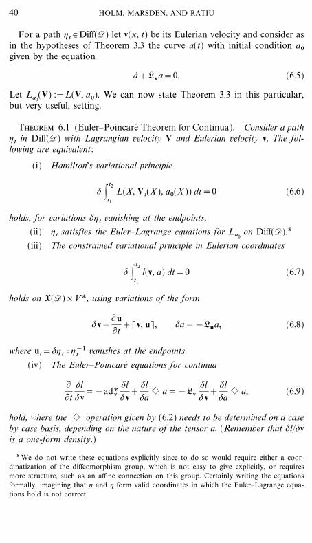
File: DISTL2 172140 . By:CV . Date:11:06:98 . Time:10:43 LOP8M. V8.B. Page 01:01Codes: 2772 Signs: 1512 . Length: 45 pic 0 pts, 190 mm
For a path 't # Diff(D) let v(x, t) be its Eulerian velocity and consider asin the hypotheses of Theorem 3.3 the curve a(t) with initial condition a0
given by the equation
a* +Lva=0. (6.5)
Let La0(V) :=L(V, a0). We can now state Theorem 3.3 in this particular,
but very useful, setting.
Theorem 6.1 (Euler�Poincare� Theorem for Continua). Consider a path't in Diff(D) with Lagrangian velocity V and Eulerian velocity v. The fol-lowing are equivalent:
(i) Hamilton's variational principle
$ |t2
t1
L(X, Vt(X ), a0(X )) dt=0 (6.6)
holds, for variations $'t vanishing at the endpoints.
(ii) 't satisfies the Euler�Lagrange equations for La0on Diff(D).8
(iii) The constrained variational principle in Eulerian coordinates
$ |t2
t1
l(v, a) dt=0 (6.7)
holds on X(D)_V*, using variations of the form
$v=�u�t
+[v, u], $a=&Lua, (6.8)
where ut=$'t b '&1t vanishes at the endpoints.
(iv) The Euler�Poincare� equations for continua
��t
$l$v
=&ad*v$l$v
+$l$a
h a=&Lv$l$v
+$l$a
h a, (6.9)
hold, where the h operation given by (6.2) needs to be determined on a caseby case basis, depending on the nature of the tensor a. (Remember that $l�$vis a one-form density.)
40 HOLM, MARSDEN, AND RATIU
8 We do not write these equations explicitly since to do so would require either a coor-dinatization of the diffeomorphism group, which is not easy to give explicitly, or requiresmore structure, such as an affine connection on this group. Certainly writing the equationsformally, imagining that ' and '* form valid coordinates in which the Euler�Lagrange equa-tions hold is not correct.

File: DISTL2 172141 . By:CV . Date:11:06:98 . Time:10:43 LOP8M. V8.B. Page 01:01Codes: 3270 Signs: 2419 . Length: 45 pic 0 pts, 190 mm
Remarks. 1. Of course, this theorem can be proven directly by imitatingthe proof of Theorem 3.1 with appropriate modifications for right represen-tations and right actions. For those used to the more concrete language ofcontinuum mechanics as opposed to that of Lie algebras, the followingstring of equalities shows that (iii) is equivalent to (iv):
0=$ |t2
t1
l(v, a) dt=|t2
t1\ $l
$v} $v+
$l$a
} $a+ dt
=|t2
t1_ $l
$v} \�u
�t&adv u+&
$l$a
} Lu a& dt
=|t2
t1
u } _&��t
$l$v
&ad*v$l$v
+$l$a
h a& dt. (6.10)
2. Similarly, one can deduce by hand the form (6.8) of the variationsin the constrained variational principle (6.7) by a direct calculation. Thisproceeds as follows. One writes the basic relation between the spatial andmaterial velocities, namely v(x, t)='* ('&1
t (x), t). One then takes the varia-tion of this equation with respect to ' and uses the definition u(x, t)=$'('&1
t (x), t) together with a calculation of its time derivative. Of course,one can also do this calculation using the inverse map '&1
t instead of ' asthe basic variable, see Holm, Marsden, and Ratiu [1986], Holm [1996a, b].
3. As we mentioned in the context of perfect fluids, the preceding sortof calculation for $v in fluid mechanics and the interpretation of thisrestriction on the form of the variations as the so-called Lin constraints isdue to Bretherton [1970].
4. The coordinate expressions for ($l�$a) h a required to completethe equations of motion are given in the next section for several choices ofa0(X ) in three dimensions. Namely, we shall discuss the choices corre-sponding to scalars, one-forms, two-forms, densities in three dimensions,and symmetric tensors. In the equations of motion, all of these quantitieswill be advected.
5. As with the general theory, variations of the action in the advectedtensor quantities contribute to the equations of motion which follow fromHamilton's principle. At the level of the action l for the Euler�Poincare�equations, the Legendre transform in the variable v alone is often non-singular, and when it is, it produces the Hamiltonian formulation ofEulerian fluid motions with a Lie�Poisson bracket defined on the dual ofthe semidirect product algebra of vector fields acting amongst themselvesby Lie bracket and on tensor fields and differential forms by the Liederivative. This is a special instance of the more general facts for Liealgebras that were discussed earlier.
41EULER�POINCARE� AND SEMIDIRECT PRODUCTS

File: DISTL2 172142 . By:CV . Date:11:06:98 . Time:10:43 LOP8M. V8.B. Page 01:01Codes: 3018 Signs: 2330 . Length: 45 pic 0 pts, 190 mm
6. As mentioned earlier, in the absence of the tensor fields a andwhen l is the kinetic energy metric, the basic Euler�Poincare� equations arethe geodesic spray equations for geodesic motion on the diffeomorphismgroup with respect to that metric. See, e.g., Arnold [1966a], Ovsienko andKhesin [1987], Zeitlin and Kambe [1993], Zeitlin and Pasmanter [1994],Ono [1995a, 1995b], and Kouranbaeva [1997] for details in particularapplications of ideal continuum mechanics.
Remarks on the Inverse Map and the Tensor Fields a for Fluids. In thecase of fluids in the Lagrangian picture, the flow of the fluid is a diffeo-morphism which takes a fluid parcel along a path from its initial position X,in a ``reference configuration'' to its current position x in the ``container'',i.e., in the Eulerian domain of flow. As we have described, this forward mapis denoted by ': X [ x. The inverse map '&1: x [ X provides the mapassigning the Lagrangian labels to a given spatial point. Interpreted aspassive scalars, these Lagrangian labels are simply advected with the fluidflow, X4 =0. In the Lagrangian picture, a tensor density in the referenceconfiguration a0(X ) (satisfying a* 0(X )=0) consists of invariant tensor func-tions of the initial reference positions and their differentials. These tensorfunctions are parameters of the initial fluid reference configuration (e.g., theinitial density distribution, which is an invariant n-form).
When viewed in the Eulerian picture as
at(x) :=('t*a0)(x)=(' t*
&1a0)(x),
i.e.,
a0(X ) :=('t*at)(X )=(' t*&1a0)(X ),
the time invariant tensor density a0(X ) in the reference configurationacquires advective dynamics in the Eulerian picture, namely
a* 0(X )=\ ��t
+Lv+ a(x, t)=0,
where Lv denotes Lie derivative with respect to the Eulerian velocity fieldv(x, t). This relation results directly from the well known Lie derivativeformula for tensor fields. (See, for example, Abraham, Marsden and Ratiu[1988].)
Mapping the time invariant quantity a0 (a tensor density function of X )to the time varying quantity at (a tensor density function of x) as explainedabove is a special case of the general way we advect quantities in V* in thegeneral theory. Specifically, we can view this advection of at as being thefluid analogue of the advection of the unit vector along the direction of
42 HOLM, MARSDEN, AND RATIU

File: DISTL2 172143 . By:CV . Date:11:06:98 . Time:10:43 LOP8M. V8.B. Page 01:01Codes: 2839 Signs: 2050 . Length: 45 pic 0 pts, 190 mm
gravity (a spatially fixed quantity) by means of the body rotation vector inthe heavy top example.
Consistent with the fact that the heavy top is a left invariant system whilecontinuum theories are right invariant, the advected tensor density at is aspatial quantity, while the advected direction of gravity is a body quantity.If we were to take the inverse map '&1 as the basic group variable, ratherthan the map ', then continuum theories would also become left invariant.
The Continuity Equation for the Mass Density. We will need to imposean additional assumption on our continuum theory. Namely, we assumethat amongst the tensor densities being advected, there is a special one,namely the mass density. This of course is a tensor density that occurs inall continuum theories. We denote this density by \d nx and it is advectedaccording to the standard principles discussed above. Thus, \ satisfies theusual continuity equation:
��t
\+div(\v)=0.
In the Lagrangian picture we have \d nx=\0(X ) d nX, where \0(X ) is themass density in the reference configuration. It will also be convenient in thecontinuum examples below to define Lagrangian mass coordinates l(X )satisfying \d nx=d nl with l4 =0. (When using Lagrangian mass coor-dinates, we shall denote the density \ as D.) We assume that \ (or D) isstrictly positive.
The Kelvin�Noether Circulation Theorem. Let C be the space of con-tinuous loops #: S1 � D in D and let the group Diff(D) act on C on the leftby (', #) # Diff(D)_C [ '# # C, where '#=' b #.
Next we shall define the circulation map K: C_V* � X(D)**. Given aone form density : # X* we can form a one form (no longer a density) bydividing it by the mass density \; we denote the result just by :�\. We letK then be defined by
(K(#, a), :)=�#
:\
. (6.11)
The expression in this definition is called the circulation the one-form :�\around the loop #.
This map is equivariant in the sense that
(K(' b #, '*
a), '*
:)=(K(#, a), :)
for any ' # Diff(D). This is proved using the definitions and the change ofvariables formula.
43EULER�POINCARE� AND SEMIDIRECT PRODUCTS

File: DISTL2 172144 . By:CV . Date:11:06:98 . Time:10:43 LOP8M. V8.B. Page 01:01Codes: 2255 Signs: 1123 . Length: 45 pic 0 pts, 190 mm
Given the Lagrangian l : X(D)_V* � R, the Kelvin�Noether quantity isgiven by (4.1) which in this case becomes
I(#, v, a)=�#
1\
$l$v
.
With these definitions of K and I, the statement of Theorem 4.1 becomesthe classical Kelvin circulation theorem.
Theorem 6.2 (Kelvin Circulation Theorem). Assume that v(x, t)satisfies the Euler�Poincare� equations for continua:
��t \
$l$v+=&Lv \ $l
$v++$l$a
h a
and a satisfies the advection relation
�a�t
+Lva=0.
Let 't be the flow of the Eulerian velocity field v, that is, vt=(d't�dt) b '&1t .
Define #t :='t b #0 and I(t) :=I(#t , vt , at). Then
ddt
I(t)=�#t
1\
$l$a
h a.
In this statement, we use a subscript t to emphasise that the operationsare done at a particular t and to avoid having to write the otherarguments, as in at(x)=a(x, t); we omit the arguments from the notationwhen convenient. Due to the importance of this theorem we shall give herea separate proof tailored for the case of continuum mechanical systems.
Proof. First we change variables in the expression for I(t):
I(t)=�#t
1\t
$l$v
=�#0
't* _ 1\t
$l$v&=�
#0
1\0
't* _ $l$v& .
Next, we use the Lie derivative formula
ddt
('t*:t)='t* \ ��t
:t+Lv:t+ ,
44 HOLM, MARSDEN, AND RATIU
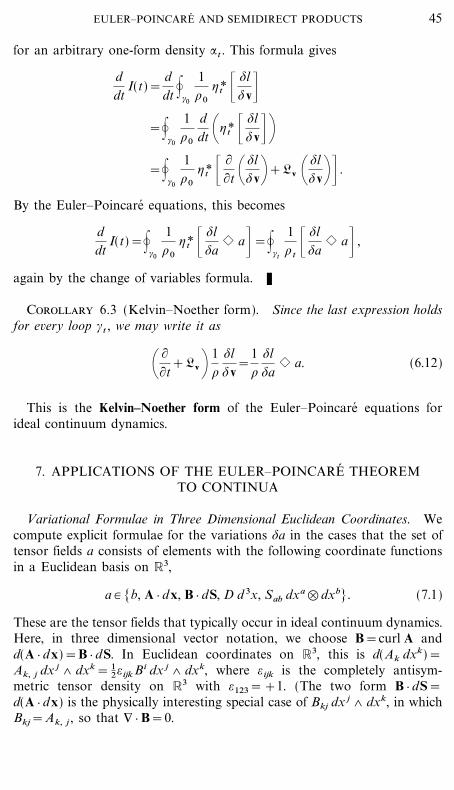
File: DISTL2 172145 . By:CV . Date:11:06:98 . Time:10:43 LOP8M. V8.B. Page 01:01Codes: 2627 Signs: 1306 . Length: 45 pic 0 pts, 190 mm
for an arbitrary one-form density :t . This formula gives
ddt
I(t)=ddt �#0
1\0
't* _ $l$v&
=�#0
1\0
ddt \'t* _ $l
$v&+=�
#0
1\0
't* _ ��t \
$l$v++Lv \ $l
$v+& .
By the Euler�Poincare� equations, this becomes
ddt
I(t)=�#0
1\0
't* _ $l$a
h a&=�#t
1\t _
$l$a
h a& ,
again by the change of variables formula. K
Corollary 6.3 (Kelvin�Noether form). Since the last expression holdsfor every loop #t , we may write it as
\ ��t
+Lv+ 1\
$l$v
=1\
$l$a
h a. (6.12)
This is the Kelvin�Noether form of the Euler�Poincare� equations forideal continuum dynamics.
7. APPLICATIONS OF THE EULER�POINCARE� THEOREMTO CONTINUA
Variational Formulae in Three Dimensional Euclidean Coordinates. Wecompute explicit formulae for the variations $a in the cases that the set oftensor fields a consists of elements with the following coordinate functionsin a Euclidean basis on R3,
a # [b, A } dx, B } dS, D d 3x, Sab dxa�dxb]. (7.1)
These are the tensor fields that typically occur in ideal continuum dynamics.Here, in three dimensional vector notation, we choose B=curl A andd(A } dx)=B } dS. In Euclidean coordinates on R3, this is d(Ak dxk)=Ak, j dx j 7 dxk= 1
2=ijkBi dx j 7dxk, where = ijk is the completely antisym-metric tensor density on R3 with =123=+1. (The two form B } dS=d(A } dx) is the physically interesting special case of Bkj dx j 7 dxk, in whichBkj=Ak, j , so that { } B=0.
45EULER�POINCARE� AND SEMIDIRECT PRODUCTS

File: DISTL2 172146 . By:CV . Date:11:06:98 . Time:10:43 LOP8M. V8.B. Page 01:01Codes: 2603 Signs: 1030 . Length: 45 pic 0 pts, 190 mm
We have seen that invariance of the set a in the Lagrangian picture underthe dynamics of v implies in the Eulerian picture that (���t+Lv ) a=0, whereLv denotes Lie derivative with respect to the velocity vector field v. Accordingto Theorem 6.1, equation (6.9), the variations of the tensor functions a at fixedx and t are also given by Lie derivatives, namely $a=&Lua, or
$b=&Lub=&u } {b,
$A } dx=&Lu (A } dx)=&((u } {) A+A j {u j) } dx
=(u_curl A&{(u } A)) } dx,
$B } dS=&Lu (B } dS)=(curl(u_B)) } dS=d($A } dx),
$D d 3x=&Lu (D d 3x)=&{ } (Du) d 3x,
$Sab dxa�dxb=&Lu (Sab dxa �dxb)
=&(ukSab, k+Skb uk, a+Skauk
, b) dxa�dxb. (7.2)
Hence, Hamilton's principle with this dependence yields
0=$ | dt l(v; b, A, B, D, Sab)
=| dt _ $l$v
} $v+$l$b
$b+$l$D
$D+$l
$A} $A+
$l$B
} $B+$l
$Sab$Sab&
=| dt _ $l$v
} \�u�t
&adv u+&$l$b
u } {b&$l$D
({ } (Du))
+$l
$A} (u_curl A&{(u } A))+
$l$B
} (curl(u_B))
&$l
$Sab(ukSab, k+Skbuk
, a+Skauk, b)&
=| dt _u } \&��t
�l�v
&ad*v$l$v
&$l$b
{b+D{$l$D
&$l
$A_curl A+A div
$l$A
+B_curl$l$B+
+uk \&$l
$SabSab, k+\ $l
$SabSkb+ , a
+\ $l$Sab
Ska+ , b+&=| dt u } _&
��t
$l$v
&ad*v$l$v
+$l$a
h a&=| dt u } _&\ �
�t+Lv+ $l
$v+
$l$a
h a& , (7.3)
46 HOLM, MARSDEN, AND RATIU

File: DISTL2 172147 . By:CV . Date:11:06:98 . Time:10:43 LOP8M. V8.B. Page 01:01Codes: 2493 Signs: 1144 . Length: 45 pic 0 pts, 190 mm
where we have consistently dropped boundary terms arising from integra-tions by parts, by invoking natural boundary conditions. Thus, for the setof tensor fields a in Eq. (7.1) we have the following Euclidean componentsof ($l�$a) h a,
\$l$a
h a+k= &
$l$b
b , k+D \ $l$D+ , k
+\&$l
$A_curl A+A div
$l$A
+B_curl$l$B+k
&$l
$SabSab, k+\ $l
$SabSkb+ , a
+\ $l$Sab
Ska+ , b. (7.4)
Stress Tensor Formulation. For example, if we assume a Lagrangian inthe form
l(v; b, A, B, D, Sab)=| d 3x L(v, {v, b, A, B, D, Sab), (7.5)
where L is a given function, then we may use Eq. (7.4) to express theEuler�Poincare� equations for continua (6.9) in this case in the momentumconservation form,
��t
$l$v
=&ad*v$l$v
+$l$a
h a O�mi
�t=&
��x j T j
i , (7.6)
with momentum density components mi , i=1, 2, 3 defined by
mi #$l$vi=
�L
�vi &�
�xk \ �L
�v i, k+ , (7.7)
and stress tensor T ji given by
T ji =mi v j&
�L
�vk, j
vk, i&
�L
�AjAi+
�L
�Bi B j&�L
�S jbSib&
�L
�SajSia
+$ ji \L&D
�L
�D&Bk �L
�Bk+ . (7.8)
Here, in the calculation of T ji , we have used the coordinate expression (6.3)
for ad*u (:�m).
Kelvin�Noether Form. The Euclidean components of the Euler�Poincare�equations for ideal continua may also be summarized in Kelvin�Noether
47EULER�POINCARE� AND SEMIDIRECT PRODUCTS

File: DISTL2 172148 . By:CV . Date:11:06:98 . Time:10:43 LOP8M. V8.B. Page 01:01Codes: 2942 Signs: 1970 . Length: 45 pic 0 pts, 190 mm
form (6.12) for advected tensor fields a in the set (7.1). We adopt the nota-tional convention of the circulation map K in Eq. (6.11) that a one formdensity can be made into a one form (no longer a density) by dividing it bythe mass density D to produce, e.g., the one form in Euclidean components(1�D)($l�$vi) dx i from the one form density $l�$v. With a slight abuse ofnotation (but in accord with the usual physics conventions) we write theformer coordinate expression as (1�D)($l�$v) } dx. We also denote the Lie-derivative relation for the continuity equation as (���t+Lv ) D d 3x=0.Then, the Euclidean components of the Euler�Poincare� equations for con-tinua in (7.3) are expressed in Kelvin�Noether form (6.12) as
\ ��t
+Lv+\ 1D
$l$v
} dx++1D
$l$b
{b } dx&{ \ $l$D+ } dx
+1D \ $l
$A_curl A&A div
$l$A+ } dx&
1D \B_curl
$l$B+ } dx
+1D \ $l
$SabSab, k&\ $l
$SabSkb+ , a
&\ $l$Sab
Ska+ , b + dxk=0, (7.9)
where the components of the variational derivatives of the Lagrangian l areto be computed according to the usual physics conventions, i.e., as com-ponents of Fre� chet derivatives as in Eq. (1.50). In physical applications,the advected Eulerian tensor fields a in (7.1) represent the buoyancy b (orspecific entropy, for the compressible case), magnetic vector potential A,magnetic field intensity B, mass density D, and Cauchy�Green strain tensorSab , respectively. Formula (7.9) is the Kelvin�Noether form of the equationof motion for ideal continua in Euclidean coordinates. This Euclidean com-ponent formula is especially convenient for direct calculations in fluiddynamics, to which we turn our attention next.
Eulerian Motion Equation for an Ideal Incompressible Fluid. In theEulerian velocity representation we consider fluid motion in an n-dimen-sional domain and define the reduced action Sred and reduced Lagrangianl(v, D) by
Sred=| dt l=| dt | d nx[ 12D |v| 2& p(D&1)]. (7.10)
This action produces the following variations at fixed x and t
1D
$l$v
=v,$l$D
=12
|v|2& p,$l$p
=&(D&1). (7.11)
48 HOLM, MARSDEN, AND RATIU
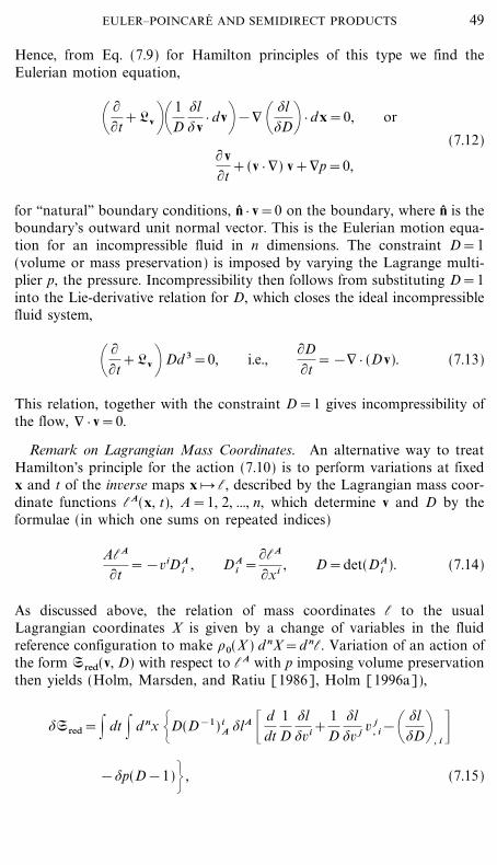
File: DISTL2 172149 . By:CV . Date:11:06:98 . Time:10:43 LOP8M. V8.B. Page 01:01Codes: 2595 Signs: 1578 . Length: 45 pic 0 pts, 190 mm
Hence, from Eq. (7.9) for Hamilton principles of this type we find theEulerian motion equation,
\ ��t
+Lv+\ 1D
$l$v
} dv+&{ \ $l$D+ } dx=0, or
(7.12)�v�t
+(v } {) v+{p=0,
for ``natural'' boundary conditions, n } v=0 on the boundary, where n is theboundary's outward unit normal vector. This is the Eulerian motion equa-tion for an incompressible fluid in n dimensions. The constraint D=1(volume or mass preservation) is imposed by varying the Lagrange multi-plier p, the pressure. Incompressibility then follows from substituting D=1into the Lie-derivative relation for D, which closes the ideal incompressiblefluid system,
\ ��t
+Lv+ Dd 3=0, i.e.,�D�t
=&{ } (Dv). (7.13)
This relation, together with the constraint D=1 gives incompressibility ofthe flow, { } v=0.
Remark on Lagrangian Mass Coordinates. An alternative way to treatHamilton's principle for the action (7.10) is to perform variations at fixedx and t of the inverse maps x [ l, described by the Lagrangian mass coor-dinate functions lA(x, t), A=1, 2, ..., n, which determine v and D by theformulae (in which one sums on repeated indices)
AlA
�t=&viDA
i , DAi =
�lA
�xi , D=det(DAi ). (7.14)
As discussed above, the relation of mass coordinates l to the usualLagrangian coordinates X is given by a change of variables in the fluidreference configuration to make \0(X ) d nX=d nl. Variation of an action ofthe form Sred(v, D) with respect to lA with p imposing volume preservationthen yields (Holm, Marsden, and Ratiu [1986], Holm [1996a]),
$Sred=| dt | d nx {D(D&1) iA $lA _ d
dt1D
$l$vi+
1D
$l$v j v j
, i&\ $l$D+ , i&
&$p(D&1)= , (7.15)
49EULER�POINCARE� AND SEMIDIRECT PRODUCTS

File: DISTL2 172150 . By:CV . Date:11:06:98 . Time:10:43 LOP8M. V8.B. Page 01:01Codes: 2598 Signs: 1758 . Length: 45 pic 0 pts, 190 mm
where d�dt=���t+(v } {) is the material derivative of Eulerian quantitiesand we again invoke natural boundary conditions when integrating byparts.
Hence, the vanishing of the coefficient of $lA in the variational formula(7.15) recovers the Euler�Poincare� equation (7.12) for the Eulerian fluidvelocity, v, by stationarity of the action (7.10) with respect to variationsof the Lagrangian mass coordinates lA(x, t). Similar arguments based onstationary variations of the action with respect to the Lagrangian mass coor-dinates lA at fixed x, t will also recover the more general Euler�Poincare�equations (7.9) from actions which depend on the velocity v and the advectedquantities in Eq. (7.1) through their dependence on the lA(x, t).
Adiabatic Compressible MHD. In the case of adiabatic compressiblemagnetohydrodynamics (MHD), the action in Hamilton's principle isgiven by
Sred=| dt l=| dt d 3x \D2
|v|2&De(D, b)&12
|B| 2+ , (7.16)
where e(D, b) is the fluid's specific internal energy, whose dependence onthe density D and specific entropy b is given as the ``equation of state'' andwhich for an isotropic medium satisfies the thermodynamic first law in theform de=&pd(1�D)+Tdb with pressure p(D, b) and temperature T(D, b).The variation of l in (7.16) is
$Sred=| dt d 3x Dv } $v&DT $b+( 12 |v|2&h) $D&B } $B. (7.17)
The quantity h=e+ p�D denotes the specific enthalpy, which thus satisfiesdh=(1�D) dp+Tdb. The Euler�Poincare� formula in the Kelvin�Noetherform (7.9) yields the MHD motion equation as
\ ��t
+Lv+ (v } dx)&T db+1D
B_curl B } dx&d \12
|v|2&h+=0, (7.18)
or, in three dimensional vector form,
�v�t
+(v } {) v+1D
{p+1D
B_curl B=0. (7.19)
By definition, the advected variables [b, B, D] satisfy the following Lie-derivative relations which close the ideal MHD system,
50 HOLM, MARSDEN, AND RATIU

File: DISTL2 172151 . By:CV . Date:11:06:98 . Time:10:43 LOP8M. V8.B. Page 01:01Codes: 2761 Signs: 1788 . Length: 45 pic 0 pts, 190 mm
\ ��t
+Lv+ b=0, or�b�t
=&v } {b,
\ ��t
+Lv+ B } dS=0, or�B�t
=curl(v_B), (7.20)
\ ��t
+Lv+ D d 3x=0, or�D�t
=&{ } (Dv),
and the function p(D, b)=D2 �e��D is specified by giving the equation ofstate of the fluid, e=e(D, b). If the condition { } B=0 holds initially, thenit holds for all time; since this constraint is preserved by the dynamicalequation for B.
Adiabatic Magneto-Elastodynamics. When nonlinear elasticity is also afactor in the MHD evolution, there is an additional Lie-derivative relation,
\ ��t
+Lv+ (Sab dxa�dxb)=0, (7.21)
leading to the dynamical equation for the advected Cauchy�Green straintensor Sab (which measures nonlinear strain in spatial coordinates),
��t
Sab=&(vkSab, k+Skb vk, a+Skavk
, b). (7.22)
In this case, additional stress terms appear in the motion equation for vthat arise from the dependence of the specific internal energy e(D, b, Sab)on the Cauchy�Green strain tensor Sab in the MHD action (7.16) when theelasticity of the medium is involved. The stress tensor per unit mass _ab isdetermined from the equation of state of such an magneto-elastic mediumby the Doyle�Erickson formula _ab#�e��Sab . The Euler�Poincare� equa-tion (7.9) for ideal magneto-elasticity is then seen to be
�vi
�t+v jv i, j+
1D
p , i+1D
B j (Bj, i&Bi, j)&(_abSib) , a&(_abSia) , b=0, (7.23)
where we have used the specific enthalpy relation for an elastic medium,dh&T db=D&1 dp+_ab dSab . Thus, adiabatic magneto-elastodynamicssummons all of the advected quantities in Eq. (7.1) and makes use of theentire Euler�Poincare� equation (7.9).
Adiabatic Compressible Maxwell Fluid Dynamics via the Kaluza�KleinConstruction. An adiabatic Maxwell fluid (MF) with (nonrelativistic)Eulerian fluid velocity v, density D, specific entropy b and pressure p(D, b)satisfies the following system of equations,
51EULER�POINCARE� AND SEMIDIRECT PRODUCTS

File: DISTL2 172152 . By:CV . Date:11:06:98 . Time:10:43 LOP8M. V8.B. Page 01:01Codes: 2751 Signs: 1831 . Length: 45 pic 0 pts, 190 mm
�v�t
+(v } {) v+1D
{p(D, b)=qm
(E+v_B),
�D�t
=&{ } (Dv),�b�t
=&(v } {) b,
(7.24)
{ } E=qm
D,�E�t
=&qm
Dv+{_B,
{ } B=0,�B�t
=&{_E.
This system consists of the motion equation for a charged fluid movingunder the combined effects of pressure gradient and Lorentz forces; thecontinuity equation for the mass density D; advection of the specificentropy, b; and Maxwell's equations for the electromagnetic fields E and Bin the moving fluid medium, whose polarizability and magnetization areneglected for simplicity. (For the physically more realistic treatment ofmoving media with electromagnetic induction in a similar framework,including relativistic effects, see Holm [1987].) The equations for D and bare the familiar advection laws. The coupling constant q�m is the charge-to-mass ratio of the fluid particles, and the electric and magnetic fields E andB are defined in terms of the scalar and vector potentials 8 and A by
E# &�A�t
{8, B#{_A. (7.25)
In the MF equations (7.24), charged fluid motion is the source for theelectromagnetic fields which act self-consistently upon the fluid through theLorentz force. We shall show that Eq. (7.24) are Euler�Poincare� equationsfor the gauge invariant action of ``Kaluza�Klein'' form given by
Sred=| dt l=| dt d 3x \12
D |v|2+12
D(A } v&8+|~ )2&De(D, b)
+12 }
�A�t
+{8 }2
&12
|{_A|2+ , (7.26)
where |~ =�%��t+v } {% for a gauge field % and e(D, b) is the fluid's specificinternal energy, which satisfies the first law of thermodynamics in the formde=&pd(1�D)+T db with pressure p(D, b) and temperature T(D, b).
This action principle fits into the general theory with the electromagneticfield variables playing the role of additional configuration variables whichare not acted on by the particle relabelling group. They obey the usualEuler�Lagrange equations, coupled to the Euler�Poincare� variables through
52 HOLM, MARSDEN, AND RATIU

File: DISTL2 172153 . By:CV . Date:11:06:98 . Time:10:43 LOP8M. V8.B. Page 01:01Codes: 2518 Signs: 1469 . Length: 45 pic 0 pts, 190 mm
the Lagrangian. In other words, the primitive unreduced Lagrangian in thiscase is of the abstract form L: TG_V*_TQ_TC � R in which G, thefluid particle relabelling group, acts trivially on the Maxwell field variablesQ and the gauge field % # C. Note that the Lagrangian in equation (7.26)is invariant under translations of %, as well as under the electromagneticgauge transformations,
A � A+{`, 8 � 8&�`��t, % � %&`, (7.27)
for an arbitary function ` of x and t.We now take variations of the action. The variation of Sred in Eq. (7.26)
may be written using the definitions of E and B, and the abbreviated notationc#A } v&8+|~ , as
$Sred=| dt d 3x _D(v+cA+c {%) } $b+\12
|v|2+12
c2&e&pD+ $D
&DT $b+\c Dv+�E�t
&{_B+ } $A+(&cD+{ } E) $8
&\�c D�t
+{ } c Dv+ $%& , (7.28)
where terms arising from integration by parts vanish for the natural bound-ary conditions given by
v } n=0, E } n=0, and n_B=0 on the boundary, (7.29)
and for variations $g(t) of g(t) vanishing at the endpoints. Stationarity ofthe action Sred in (7.26) under variation of the gauge field % gives theconservation law,
\ ��t
+v } {+ c=0 via the continuity equation,
(7.30)�D�t
+{ } (Dv)=0,
Hence, we may set c=q�m in equation (7.28) and then acquire the twoMaxwell equations with sources from stationarity of the action Sred undervariations of A and 8. Once the flow velocity v is known, the relationc=q�m determines the gauge function % by ``quadrature,'' from the defini-tions of c and |~ as
|~ #�%�t
+v } {%=qm
+8&A } v. (7.31)
53EULER�POINCARE� AND SEMIDIRECT PRODUCTS

File: DISTL2 172154 . By:CV . Date:11:06:98 . Time:10:43 LOP8M. V8.B. Page 01:01Codes: 2471 Signs: 1159 . Length: 45 pic 0 pts, 190 mm
The remaining variations of Sred in [v, D, b] for the Euler�Poincare�dynamics collect into the Kelvin�Noether form of Eq. (7.9) as
\ ��t
+v } {+\ 1D
$l$v++
1D
$l$v j {v j+
1D
$l$b
{b&{$l$D
=0. (7.32)
Specifically, we have
\ ��t
+v } {+ (v+cA+c {%)+(vj+cAj+c% , j) {v j
&T {b&{ \12
|v|2+12
c2&e&pD+=0. (7.33)
Using the fundamental vector identity of fluid dynamics in three dimensions,
(b } {) a+aj {b j=&b_({_a)+{(a } b), (7.34)
with, in this case, b=v and a=D&1 $l�$v, casts the Euler�Poincare� equation(7.32) into its equivalent ``curl'' form,
��t \
1D
$l$v+&v_{_\ 1
D$l$v++
1D
$l$b
{b+{ \v }1D
$l$v
&$l$D+=0. (7.35)
Similarly, applying the same vector identity with b=v and a=c(A+{%) inthe Maxwell fluid motion equation (7.33) yields,
�v�t
+(v } {) v+1D
{p=c \&�A�t
&{8+v_({_A)+=
qm
(E+v_B), (7.36)
where we have used the thermodynamic first law. Thus we find theMaxwell fluid motion law��the first among the equations in (7.24)��aftersetting c=q�m and using the definitions of the electromagnetic fields E andB in terms of the potentials A and 8.
Theorem 7.1 (Kelvin Circulation Theorem for the Maxwell Fluid). Bythe MF motion equation (7.36) and the thermodynamic first law, we have
dIdt
=�#t
T db, (7.37)
54 HOLM, MARSDEN, AND RATIU

File: DISTL2 172155 . By:CV . Date:11:06:98 . Time:10:43 LOP8M. V8.B. Page 01:01Codes: 2407 Signs: 1370 . Length: 45 pic 0 pts, 190 mm
where the circulation integral is given by
I#�#t\v+
qm
A+ } dx,
for a curve #t which moves with the fluid velocity v.
Proof. The proof is the same as for Theorem 6.2; although it is alsoimmediately seen from the motion equation (7.33) after substitutingD&1 $l�$v=v+c(A+{%) and D&1 $l�$b=&T. K
Corollary 7.2 (Potential Vorticity Convection for the Maxwell-Fluid).Stokes' theorem, advection of specific entropy b and the continuity equationtogether imply convection of potential vorticity for the adiabatic Maxwellfluid,
�q�t
+v } {q#dqdt
=0 with q#1D
{b } curl \v+qm
A+ . (7.38)
Remark. The equation dq�dt=0 for convection of potential vorticity fora general Lagrangian with dependence l(v, b, D), with
q=1D
{b } curl \ 1D
$l$v+ , (7.39)
may also be proven directly from the ``curl'' form of the Kelvin�NoetherEq. (7.35) in three dimensions, by taking the scalar product of its curl with{b and applying the continuity equation for D.
Alternative Interpretations of the Maxwell Fluid Formulation. Note thatthe first line of the Euler�Poincare� motion equation (7.36) for Maxwellfluids persists, when the electromagnetic energy terms are dropped from theMF Lagrangian in Eq. (7.26), to give the action
Sred =| dt l
=| dt d 3x( 12D |v| 2+ 1
2D(A } v&8+|~ )2&De(D, b)). (7.40)
The Euler�Poincare� equation which results from this action is
�v�t
+(v } {) v+1D
{p=c \&�A�t
&{8+v_({_A)+ . (7.41)
55EULER�POINCARE� AND SEMIDIRECT PRODUCTS

File: DISTL2 172156 . By:CV . Date:11:06:98 . Time:10:43 LOP8M. V8.B. Page 01:01Codes: 3244 Signs: 2674 . Length: 45 pic 0 pts, 190 mm
The Kelvin Theorem 7.1 and its potential vorticity Corollary 7.2 also persistfor the dynamics derived from this truncated action. The ``Lorentz force''terms in Eq. (7.41) in terms of A and 8 arise purely from the Kaluza�Kleincoupling term��the second term in the integrand of the action Sred inEq. (7.40). These ``Lorentz forces'' may be interpreted physically as non-inertial forces resulting from having moved into a frame of reference witha prescribed velocity given by A(x, t). The velocity v then represents fluidflow relative to this noninertial frame. This situation reduces to Faradaydriving of the fluid (Faraday [1831]), when A(x, t) corresponds to a rigidmotion of the fluid container. For a simple example, set c= f0 ; {8=0;and A= 1
2 z_x. Then cv_({_A)=v_f0 z gives the Coriolis force and vcorresponds to fluid velocity in a uniformly rotating reference frame withconstant angular velocity f0 . This is the typical situation in geophysicalfluid dynamics.
Alternatively, the right-hand side of Eq. (7.41) may be interpreted as avortex force arising from a given wave field at the surface of an incom-pressible fluid (for D=1), as in Craik and Leibovich [1976] (see alsoHolm [1996b]). The Craik�Leibovich equations are formally identical toEq. (7.41) when A is identified as the prescribed mean Stokes drift velocitydue to the presence of the wave field.
Fluid motion equations of the same form as (7.41) also appear in thegeneralized Lagrangian-mean (GLM) formulation of wave, mean-flowinteraction theories (see Andrews and McIntyre [1978a, b]), in which |~is the Doppler-shifted frequency of a wave packet interacting with aLagrangian-mean flow of velocity v, and A is the prescribed pseudomomentumper unit mass of the wave. For a discussion of self-consistent Lie�PoissonHamiltonian theories of wave, mean-flow interaction in a similar form, seeGjaja and Holm [1996].
Geodesic Motion and the Kaluza�Klein Construction for IncompressibleFluids. Hamilton's principle for the action in the ``minimal coupling'' form
S$=| dt l=| dt d 3x \12
D |v|2+qm
DA } v&qm
D8&De(D, b)+ , (7.42)
yields the same Euler�Poincare� equation (7.41) as results from Hamilton'sprinciple for the Kaluza�Klein action in Eq. (7.40). Thus, we see that byintroducing the auxiliary gauge field, %, the Kaluza�Klein construction ren-ders the minimal coupling form of the action for fluid dynamics quadraticin the velocity, while preserving its corresponding Euler�Poincare� equation.The Kaluza�Klein construction for charged particle mechanics is discussedin Marsden and Ratiu [1994]. The historical references are Kaluza[1921], Klein [1926] and Thirry [1948].
56 HOLM, MARSDEN, AND RATIU
File: DISTL2 172157 . By:CV . Date:11:06:98 . Time:10:43 LOP8M. V8.B. Page 01:01Codes: 2954 Signs: 2319 . Length: 45 pic 0 pts, 190 mm
In the incompressible case, when the Kaluza�Klein action is taken to be
Sred=| dt l=| dt d 3x( 12D |v|2+ 1
2 D(A } v&8+|~ )2& p(D&1)), (7.43)
for arbitrary prescribed functions A and 8, the resulting Euler�Poincare�equation (i.e., Eq. (7.41) with D=1) represents geodesic motion on thegroup of volume-preserving diffeomorphisms with respect to the conservedkinetic-energy metric given by
&v&2=| d 3x( 12 |v|2+ 1
2 (A } v&8+|~ )2), (7.44)
where c#A } v&8+|~ is an advected quantity, dc�dt=0. This observationextends the geodesic property of incompressible ideal fluid flows establishedin Arnold [1966a] to the case of incompressible Maxwell fluid flows, aswell as to the case of incompressible ideal fluid flows in an arbitrarily movingreference frame. From the Euler�Poincare� point of view, this extensionenlarges the particle relabelling group G from the group of diffeomorphismsto the group of automorphisms of the single particle Kaluza�Klein bundle.The total system for the incompressible Maxwell fluid flows is then geodesicmotion on the product of this automorphism group with the Maxwell fieldsthemselves. We believe that a similar extension may be involved in theresults of Ono [1995a, 1995b].
We should also remark that when one has equations in geodesic form,one can make use of all the attendant geometry to obtain additional inter-esting results. Examples of this applied to questions of stability and con-jugate points are given in the works of Misiolek listed in the references.
8. APPROXIMATE MODEL FLUID EQUATIONS WHICHPRESERVE THE EULER�POINCARE� STRUCTURE
The preceding section demonstrates the applicability of the Euler�Poincare� theorem for ideal continua when the equations of motion aregiven. Here we discuss approximate fluid models which preserve the Euler�Poincare� structure, and are obtained by making asymptotic expansions andother approximations in Hamilton's principle for a given set of modelequations. As examples, in this section we first discuss the derivation of thequasi-geostrophic approximation in geophysical fluid dynamics from anapproximation of Hamilton's principle for the rotating shallow water equa-tions. Next, we discuss the Boussinesq approximation for dispersive waterwaves in one dimension. As an example of the type of ``bonus'' which may
57EULER�POINCARE� AND SEMIDIRECT PRODUCTS

File: DISTL2 172158 . By:CV . Date:11:06:98 . Time:10:43 LOP8M. V8.B. Page 01:01Codes: 2590 Signs: 1940 . Length: 45 pic 0 pts, 190 mm
appear in making simplifying approximations while preserving mathe-matical structure, we derive the integrable Camassa�Holm equation(Camassa and Holm [1993], Camassa, Holm and Hyman [1994], Alberet al. [1994, 1995, 1997]), by making asymptotic approximations in theHamilton's principle for the Boussinesq equations. The Camassa�Holmequation in one dimension is a completely integrable partial differen-tial equation for dispersive water waves that was actually discovered bymaking structure preserving approximations of this type. This equationturns out to describe geodesic motion on the group of diffeomorphisms ofeither the real line or the periodic interval, with metric given by the H1
norm of the velocity. We also derive a multidimensional analogue of theone-dimensional Camassa�Holm equation by invoking the n-dimensionalversion of this geodesic property. There are also other potential advantagesof making structure preserving approximations, e.g., for numerical integra-tions. However, discussion of these other advantages is deferred to anotherplace. (See Marsden and Wendlandt [1997], Wendlandt and Marsden[1997], and Marsden, Patrick, and Shkoller [1997] for recent advances inthis direction.)
Rotating Shallow Water Dynamics as Euler�Poincare� Equations. Wefirst consider dynamics of rotating shallow water (RSW) in a two-dimen-sional domain with horizontal coordinates x=(x1 , x2). RSW motion isgoverned by the following nondimensional equations for horizontal fluidvelocity v=(v1 , v2) and depth D,
=ddt
v+ f z_v+{�=0,�D�t
+{ } Dv=0, (8.1)
with notation
ddt
#\ ��t
+v } {+ and �#\D&B=F + . (8.2)
These equations include variable Coriolis parameter f =f (x) and bottomtopography B=B(x).
The dimensionless scale factors appearing in the RSW equations (8.1)and (8.2) are the Rossby number = and the rotational Froude number F,given in terms of typical dimensional scales by
==V0
f0 L<<1 and F=
f 20L2
gB0
=O(1). (8.3)
58 HOLM, MARSDEN, AND RATIU
File: DISTL2 172159 . By:CV . Date:11:06:98 . Time:10:43 LOP8M. V8.B. Page 01:01Codes: 3114 Signs: 2264 . Length: 45 pic 0 pts, 190 mm
The dimensional scales (B0 , L, V0 , f0 , g) denote equilibrium fluid depth,horizontal length scale, horizontal fluid velocity, reference Coriolis param-eter, and gravitational acceleration, respectively. Dimensionless quantitiesin Eq. (8.1) are unadorned and are related to their dimensional counter-parts (primed), according to
v=V0v, x$=Lx, t$=\ LV0+ t, f $= f0 f,
(8.4)
B$=B0B, D$=B0D, and D$&B$=B0(D&B).
Here, dimensional quantities are: v$, the horizontal fluid velocity; D$, thefluid depth; B$, the equilibrium depth; and D$&B$, the free surface elevation.
For barotropic horizontal motions at length scales L in the ocean, say,for which F is order O(1)��as we shall assume��the Rossby number = istypically quite small (=<<1) as indicated in Eq. (8.3). Thus, =<<1 is anatural parameter for making asymptotic expansions. For example, weshall assume |{f |=O(=) and |{B|=O(=), so we may write f =1+=f1(x)and B=1+=B1(x). In this scaling, the leading order implications of equa-tion (8.1) are v=z_{� and { } v=0. This is geostrophic balance.
A simple calculation using Eq. (7.12) shows that the RSW equations(8.1) arise as Euler�Poincare� equations from Hamilton's principle withaction SRSW ,
SRSW =| dt lRSW
=| dt | dx1 dx2 _Dv } R(x)&(D&B)2
2=F+
=2
D |v|2& , (8.5)
where curl R(x)#f (x) z yields the prescribed Coriolis parameter. TheRSW equations (8.1) themselves can be regarded as being derived fromasymptotics in Hamilton's principle for three dimensional incompressiblefluid motion, see Holm [1996a]. However, this viewpoint is not pursuedfurther here, as we proceed to describe the relation of RSW to thequasigeostrophic approximation of geophysical fluid dynamics.
Quasi-geostrophy. The quasi-geostrophic (QG) approximation is a use-ful model in the analysis of geophysical and astrophysical fluid dynamics,see, e.g., Pedlosky [1987]. Physically, QG theory applies when the motionis nearly in geostrophic balance, i.e., when pressure gradients nearlybalance the Coriolis force in a rotating frame of reference, as occurs inmeso- and large-scale oceanic and atmospheric flows on Earth. Mathemati-cally, the simplest case is for a constant density fluid in a planar domainwith Euclidean coordinates x=(x1 , x2). QG dynamics for this case is
59EULER�POINCARE� AND SEMIDIRECT PRODUCTS

File: DISTL2 172160 . By:CV . Date:11:06:98 . Time:10:43 LOP8M. V8.B. Page 01:01Codes: 2793 Signs: 1969 . Length: 45 pic 0 pts, 190 mm
expressed by the following nondimensional evolution equation for the stream-function � of the incompressible geostrophic fluid velocity v=z_{�,
�({�&F�)�t
+[�, 2�]+;���x1
=0. (8.6)
Here 2 is the Laplacian operator in the plane, F denotes rotationalFroude number, [a, b]#�(a, b)��(x1 , x2) is the Jacobi bracket (Jacobian)for functions a and b defined on R2 and ; is the gradient of the Coriolisparameter, f, taken as f =1+;x2 in the ;-plane approximation, with con-stant ;. (Neglecting ; gives the f-plane approximation of QG dynamics.)The QG equation (8.6) may be derived from an asymptotic expansion ofthe RSW equations (8.1) by truncating at first order in the Rossby number,cf. Pedlosky [1987]. Equation (8.6) may be written equivalently in termsof the potential vorticity, q, as in Eq. (7.38),
�q�t
+v } {q=0, where q#2�&F�+ f for QG. (8.7)
This form of QG dynamics expresses its basic property of potential vor-ticity conservation on geostrophic fluid parcels.
The QG approximation to the RSW equations introduces ``quasi-geostrophic particles'' which move with geostrophic velocity v=z_{�and, thus, trace the geostrophic component of the RSW fluid flow. TheseQG fluid trajectories are described as functions of Lagrangian mass coor-dinates l=(l1 , l2) given by x(l, t) in the domain of flow.
Hamilton's Principle Derivation of QG as Euler�Poincare� equations. Asin Holm and Zeitlin [1997], we consider the following action for QGwritten in the Eulerian velocity representation with the integral operator(1&F2&1),
Sred =| dt l
=| dt | dx1 dx2 _=2
Dv } (1&F2&1) v+Dv } R(x)&�(D&1)& . (8.8)
This choice can be found as an asymptotic approximation of the RSWaction SRSW in Eq. (8.5), in the limit of small wave amplitudes of orderO(=2) and constant mean depth to the same order, when the wave elevationis determined from the fluid velocity by inverting the geostrophic relation,v=z_{�. The variational derivatives of the reduced Lagrangian Sred atfixed x and t are
60 HOLM, MARSDEN, AND RATIU

File: DISTL2 172161 . By:CV . Date:11:06:98 . Time:10:43 LOP8M. V8.B. Page 01:01Codes: 2330 Signs: 1328 . Length: 45 pic 0 pts, 190 mm
1D
$l$v
=R+= _v&F
22&1v&
F
2D2&1(Dv)& ,
$l$D
==2
v } (1&F2&1) v+v } R&�, (8.9)
$l$�
=&(D&1),
where we have used the symmetry of the Laplacian operator and assumedno contribution arises from the boundary when integrating by parts. Forexample, we may take the domain to be periodic. Hence, the Euler�Poincare� equation (7.12) for action principles of this type and the funda-mental vector identity (7.34) combine to give the Eulerian QG ``motionequation,''
=��t
(1&F2&1) v&v_curl(=(1&F2&1) v+R)
+{ \�+=2
v } (1&F2&1) v+=0, (8.10)
upon substituting the constraint D=1, imposed by varying �. The curl ofthis equation yields
�q�t
+v } {q+q{ } v=0, (8.11)
where the potential vorticity q is given by
q== z } curl(1&F2&1) v+ f==(2�&F�)+ f, (8.12)
with
f#z } curl R=1+;x2 , (8.13)
and ; is assumed to be of order O(=). The constraint D=1 implies { } v=0(from the kinematic relation �D��t+{ } Dv=0) and when v=z_{� issubstituted, the equation for q=2�&F�+ f yields the QG potentialvorticity convection equation (8.7). Thus, the QG approximation followsas the Euler�Poincare� equation for an asymptotic expansion of the actionfor the RSW equations when the potential energy is modelled by invertingthe geostrophic relation. The same QG equation follows upon recasting theaction (8.8) in the Kaluza�Klein form (7.43) for incompressible fluids,
61EULER�POINCARE� AND SEMIDIRECT PRODUCTS

File: DISTL2 172162 . By:CV . Date:11:06:98 . Time:10:43 LOP8M. V8.B. Page 01:01Codes: 2293 Signs: 1411 . Length: 45 pic 0 pts, 190 mm
Sred =| dt l
=| dt dx1 dx2 _=2
Dv } (1&F2&1) v+12
D(R } v+|~ )2&�(D&1)& ,
(8.14)
where |~ is defined as |~ =d%�dt=�%��t+v } {% for the gauge field %, as inthe case of the Maxwell fluid. Thus, the QG motion equation (8.10) withthe beta-effect (included in R) describes geodesic motion on the group ofarea-preserving diffeomorphisms with respect to the conserved kinetic-energy metric given by
&v&2=| dx1 dx2 _ =2
v } (1&F2&1) v+12
(R } v+|~ )2& , (8.15)
where c$#R } v+|~ is an advected quantity, dc$�dt=0. This observationfrom the Euler�Poincare� viewpoint confirms the geodesic interpretation ofthe QG equations for motion in the ;-plane established in Zeitlin andPasmanter [1994].
1D Boussinesq Dispersive Shallow Water Equations. For one dimen-sional shallow water motion with prescribed mean depth B(x) we choosethe following action
Sred=| dt l=| dt dx _12
Dv2+:2
2(Dv)2
x&g2
(D&B(x))2& , (8.16)
in which g and :2 are constants and subscript x denotes partial derivative.The second term, proportional to :2, represents the kinetic energy due tovertical motion. The last term is the potential energy. Recall that thesurface elevation h#D&B(x) satisfies �h��t=&(Dv)x for shallow waterdynamics in one dimension. Thus, the last two terms are analogous to theLagrangian
:2
2 \�h�t+
2
&g2
h2.
This is the Lagrangian for a harmonic oscillator whose displacement isgiven by the surface elevation h and whose natural frequency is - g�:. For
62 HOLM, MARSDEN, AND RATIU

File: DISTL2 172163 . By:CV . Date:11:06:98 . Time:10:43 LOP8M. V8.B. Page 01:01Codes: 2433 Signs: 1599 . Length: 45 pic 0 pts, 190 mm
the choice of action in equation (8.16) and for boundary conditions suchthat vx � 0 as |x| � �, the variation is
$Sred=| dt dx _D(v&:2(Dv)xx) $v+\v2
2&:2v(Dv)xx& gh+ $D& .
(8.17)
The Kelvin�Noether form of the Euler�Poincare� equations in (7.12) thengives
0=\ ��t
+Lv+\ 1D
$l$v
dx+&d \ $l$D+
=_ ��t
(v&:2(Dv)xx)+vvx+ ghx& dx. (8.18)
Upon inserting the one-dimensional continuity equation into the :2 termand rearranging slightly, we find the system of equations
�v�t
+vvx+ ghx+:2 �2hx
�t2 =0,�h�t
+(hv+B(x) v)x=0, (8.19)
the second of which is just a restatement of continuity. According toWhitham [1974] these equations were favored by Boussinesq, who firstformulated them by using the method of asymptotic expansions. Here wesee that the Boussinesq shallow water equations (8.19) are also Euler�Poincare� equations on Diff(R) derived from the action (8.16). The termproportional to :2 in Eq. (8.19) arises from the kinetic energy due to verti-cal motion in the action (8.16) and produces the wave dispersion respon-sible for solitary wave solutions of these equations.
1D Camassa�Holm Equation for Peakons. In the limit that the potentialenergy gh2�2 is negligible compared to the kinetic energy (e.g., for weakgravity, or small surface elevation), we may ignore the last term in theaction (8.16) for the Boussinesq equations in one dimension, set D=B(x)in the other terms and rescale to :2=1, conforming to the notation inCamassa and Holm [1993]. We thereby obtain the following simplifiedexpression for the shallow water action in this regime,
Sred=| dt dx B(x) ( 12v2+ 1
2v2x). (8.20)
63EULER�POINCARE� AND SEMIDIRECT PRODUCTS
File: DISTL2 172164 . By:CV . Date:11:06:98 . Time:10:43 LOP8M. V8.B. Page 01:01Codes: 2724 Signs: 2082 . Length: 45 pic 0 pts, 190 mm
For this action, when we also assume B(x)=1 (for constant bottomtopography) Hamilton's principle implies simply
0=$Sred=| dt l=| dt dx(v&vxx) $v, (8.21)
for vanishing boundary conditions for vx on the real line as |x| � �.Hence, $l�$v=v&vxx and the basic Euler�Poincare� equations for this casereduce to
��t
(v&vxx)=&adv*(v&vxx)=&v(v&vxx)x&2(v&vxx) vx . (8.22)
This is the }=0 case of the completely integrable partial differential equa-tion derived by Camassa and Holm [1993],
��t
(v&vxx)+2}vx=&3vvx+2vxvxx+vvxxx . (8.23)
For }=0, this equation admits ``peakon'' solutions. The peakons aresolitons which interact elastically and possess a peak, at which thederivative vx reverses sign. The simplest case is the single peakon, which isa solitary travelling wave solution given by v(x, t)=c0 exp &|x&c0 t|,with a constant wave speed c0 . The multipeakon solutions of theCamassa�Holm equation are obtainable from its associated Lax pair andlinear isospectral problem, as shown in Camassa and Holm [1993].
Being basic Euler�Poincare� , Eq. (8.22) describes geodesic motion.Camassa and Holm [1993] note that the integrable dynamics of Npeakons interacting nonlinearly via Eq. (8.22) reduces to finite dimensionalgeodesic motion on a manifold with N corners. This geodesic property per-sists to infinite dimensions and although the equation was originallyintended to be an approximation of shallow water motion, it turns outEq. (8.22) is also the geodesic spray equation for motion on the group ofdiffeomorphisms of the real line with metric given by the H1 norm of v, seeKouranbaeva [1997]. The }{0 case of the Camassa�Holm equation(8.23) may be obtained formally by shifting (v&vxx) by } in Eq. (8.22) andretaining homogeneous boundary conditions for (v&vxx) as |x| � �. Thecorresponding statement about geodesic motion for }{0, however, israther more technical than for }=0 and involves the Gel'fand�Fuchscocycle and the Bott�Virasoro group, see Misiolek [1997] for details. SeeAlber et al. [1994, 1995, 1997] for discussions of the periodic solutions of
64 HOLM, MARSDEN, AND RATIU

File: DISTL2 172165 . By:CV . Date:11:06:98 . Time:10:43 LOP8M. V8.B. Page 01:01Codes: 2780 Signs: 1883 . Length: 45 pic 0 pts, 190 mm
the Camassa�Holm equation and a related integrable shallow water equa-tion in the Dym hierarchy,
2}vx=��t
vxx+2vxvxx+vvxxx . (8.24)
This equation is the ``high wave number limit'' of the Camassa�Holm equa-tion (8.23).
Higher-Dimensional Camassa�Holm Equation. As we have seen, theCamassa�Holm (CH) equation in one dimension describes geodesicmotion on the diffeomorphism group with respect to the metric given bythe H1 norm of the Eulerian fluid velocity. Thus, a candidate for itsn-dimensional incompressible generalization should be the Euler�Poincare�equation that follows from the Lagrangian given by the H1 norm of thefluid velocity in n dimensions, subject to volume preservation (for n{1),
Sred=| dt l=| dt |M
d nxD2
(v ivi+:2v , ji v i
, j)& p(D&1), (8.25)
where M is the domain of the fluid and where we have restored the length-scale, or aspect-ratio parameter, :. Varying this action at fixed x and tgives
$Sred=| dt |M
d nx[(vivi+:2v , ji v i
, j) $D&(D&1) $p
+(Dvi&:2�j (Dv , ji )) $vi]+:2 | dt �
�M
d n&1x n j (Dv , ji $vi),
(8.26)
whose natural boundary conditions on �M are
v } n=0 and (n } {) v & n, (8.27)
where & denotes ``parallel to'' in the second boundary condition, which ofcourse is not imposed when :2 is absent. (Recall that $v in Eq. (8.26) isarbitrary except for being tangent on the boundary. This tangency, alongwith the second condition in Eq. (8.27) is sufficient for the boundaryintegral in Eq. (8.26) to vanish.)
Another set of boundary conditions which will guarantee the vanishingof the boundary term in (8.26) is that v=0 on �M (and correspondingly,$v=0 on �M).
An interesting difficulty with the boundary conditions (8.27) is that theydo not form a Lie algebra unless the boundary is flat. We shall correct thisdifficulty shortly with the inclusion of the second fundamental form of theboundary. (See the section ``The Riemannian CH equations'' below.)
65EULER�POINCARE� AND SEMIDIRECT PRODUCTS
File: DISTL2 172166 . By:CV . Date:11:06:98 . Time:10:43 LOP8M. V8.B. Page 01:01Codes: 2880 Signs: 1849 . Length: 45 pic 0 pts, 190 mm
By Eq. (7.9) or (7.32), the Euler�Poincare� equation for the action Sred
in Eq. (8.25) is
\ ��t
+v } {+ (v&:2 2v)+(vj&:2 2vj) {v j&{ \12
|v|2+:2
2|{v| 2& p+=0,
(8.28)
where ({v) ij=v i
, j #�vi��x j, |{v| 2#v i, jv
, ji =tr({v } {vT) and superscript
( v )T denotes transpose. We have also used the constraint D=1, whichas before implies incompressibility via the continuity equation for D. Requir-ing the motion equation (8.28) to preserve div v=0 implies a Poisson equa-tion for the pressure p with a Neumann boundary condition, which isobtained just as in the case of incompressible ideal fluid dynamics by takingthe normal component of the motion equation evaluated at the boundary.
Properties of the Camassa�Holm Equation. Since the CH action Sred in(8.25) is translation invariant, the Noether theorem ensures the CH equa-tion (8.28) conserves a momentum. In fact, by the stress tensor formulae(7.6)�(7.8), Eq. (8.28) may be rewritten as
�mi
�t=&
��x j T j
i . (8.29)
In this case, the momentum density mi , i=1, 2, 3 defined in Eq. (7.7) isgiven by
mi #$l$vi }D=1
=vi&:2 2v i , (8.30)
and the stress tensor T ji defined in Eq. (7.8) is given by
T ji=(vi&:2 2vi) v j&:2vk
, iv, jk +$ j
i p. (8.31)
Thus, Eq. (8.29) implies conservation of the total momentum,M=�M m d 3x, provided the normal component of the stress tensor T j
i
vanishes on the boundary.Since the CH equation (8.28) is Euler�Poincare� , it also has a corre-
sponding Kelvin�Noether circulation theorem. Namely, cf. Eq. (8.32),
ddt �#t
(v&:2 2v) } dx=0, (8.32)
for any closed curve #t that moves with the fluid velocity v. This expressionfor the Kelvin�Noether property of the CH equation in 3D is reminiscentof corresponding expressions in wave, mean-flow interaction theory. Thiscorrespondence suggests a physical interpretation of the :2 term in theKelvin�Noether circulation integral as a Lagrangian mean closure relation
66 HOLM, MARSDEN, AND RATIU

File: DISTL2 172167 . By:CV . Date:11:06:98 . Time:10:43 LOP8M. V8.B. Page 01:01Codes: 2746 Signs: 1884 . Length: 45 pic 0 pts, 190 mm
for the pseudomomentum of the high frequency (i.e., rapidly fluctuating,turbulent) components of the flow. In this interpretation, : corresponds tothe typical length scale at which these high frequency components becomeimportant. See Foias, Holm, and Titi [1998] for more discussion of usingthe 3D CH Eq. (8.28) as the basis for a turbulence closure model.
In three dimensions, we may use the vector identity (7.34) to re-expressthe CH motion equation (8.28) in its ``curl' form, as
��t
(1&:2 2) v&v_({_(1&:22) v)
+{ \v } (1&:22) v&12
|v|2&:2
2|{v|2+ p+=0. (8.33)
The inner product of v with this equation then implies conservation ofenergy,
E= 12|
M
d 3x(v } (1&:22) v)= 12| d 3x( |v|2+:2 |{v|2), (8.34)
upon integrating by parts and using the boundary conditions (8.27).Naturally, this energy is also conserved in n dimensions. In fact, Legendretransforming the action (8.25) gives the following Hamiltonian (stillexpressed in terms of the velocity, instead of the momentum densitym=$l�$v),
H=|M
d nx _D2
( |v| 2+:2 |{v|2)+ p(D&1)& . (8.35)
Thus, when evaluated on the constraint manifold D=1, the Lagrangianand the Hamiltonian for the CH equation coincide in n dimensions. (This,of course, is not unexpected for a stationary principle giving rise togeodesic motion.)
The curl of the 3D Camassa�Holm motion equation (8.33) yields
��t
q=q } {v&v } {q#[v, q], where q#curl(v&:2 2v), (8.36)
and we have used incompressibility and commutativity of the divergenceand Laplacian operators. Thus, v is the transport velocity for thegeneralized vorticity q and the ``vortex stretching'' term q } {v involves {v,whose L2 norm is controlled by the conservation of energy in Eq. (8.34).Boundedness of this norm will be useful in future analytical studies of the3D Camassa�Holm equation; for example, in the investigation of theLiapunov stability properties of its equilibrium solutions.
67EULER�POINCARE� AND SEMIDIRECT PRODUCTS

File: DISTL2 172168 . By:CV . Date:11:06:98 . Time:10:43 LOP8M. V8.B. Page 01:01Codes: 3044 Signs: 2188 . Length: 45 pic 0 pts, 190 mm
3D Periodic CH Motion. In a three-dimensional periodic domain, theconserved energy E in Eq. (8.34) may also be expressed as
E= 12 |
M
d 3x( |v| 2+:2 |curl v|2), (8.37)
upon integrating by parts and using div v=0. Thus, in the 3D periodiccase, the CH energy E may be interpreted as the sum of the kinetic energyand the enstrophy (i.e., the L2 norm of vorticity) of the Euler fluid.
The inner product of the generalized vorticity q with the motion equa-tion (8.33) implies conservation of helicity, for three dimensional periodicmotion. Namely, the quantity
4#|M
d 3x(1&:22) v } curl(1&:22) v (helicity), (8.38)
is also a constant of motion for three-dimensional periodic CH motion.From the CH vorticity equation (8.36), we see that steady 3D solutions
of the CH equation (denoted with subscript e for ``equilibrium'') arecharacterized by the vector-field commutation relation [ve , qe]=0. Thus,the velocity of a steady CH flow ve generates a volume preserving dif-feomorphism that leaves invariant its corresponding steady generalizedvorticity qe . For example, the CH Beltrami flows for Eq. (8.33) are charac-terized by ve=+qe , for a constant +. The CH Beltrami flows verify theinvariance property; hence, they are steady. These steady solutions are alsocritical points of the sum E+4�2+ of the energy E in Eq. (8.37) and 1�2+times the conserved helicity in Eq. (8.38). Hence, they are relative equi-librium solutions of the CH equation. The CH Beltrami flows are divergen-celess vector eigenfunctions of the product of the curl operator and theHelmholtz operator, (1&:22). They are the CH analogues of ``ABC flows''for the ideal Euler fluid.
Constitutive Properties of the CH ``Fluid.'' Physically, conservation ofthe energy in Eq. (8.37) means that the CH fluid can exchange energybetween its translational, and its rotational and shear motions. One mayask, what constitutive relation describes such a fluid?
One may verify directly that the 3D Camassa�Holm equation (8.28) inCartesian coordinates implies the following formula for the ``geodesicspray'' form of the CH equations in 3D:
(1&:22) \ ��t
+v } {+ vi
=:2(2vj)(v j, i&v , j
i )&�
�x j _\p&:2
2v i
, kv , ki + $ j
i +2:2v j, kv , k
i & . (8.39)
68 HOLM, MARSDEN, AND RATIU

File: DISTL2 172169 . By:CV . Date:11:06:98 . Time:10:43 LOP8M. V8.B. Page 01:01Codes: 3189 Signs: 2414 . Length: 45 pic 0 pts, 190 mm
In vector notation, this is
(1&:22) \ ��t
+v } {+ v
=:2(2v)_curl v&div _\p&:2
2|{v|2+ I� +2:2 {v } {vT& , (8.40)
where I� is the unit tensor. Viewed this way, the CH fluid acceleration dv�dtis nonlocal, nonlinear, and (as we know from the general Euler�Poincare�theory) geodesic. Foias, Holm, and Titi [1998] show, among other things,that the geodesic spray equation (8.40) may be rearranged into aviscoelastic constitutive relation of Jeffreys type.
Discussion. The essential idea of the CH equation is that its specificmomentum (i.e., its momentum per unit mass) is transported by a velocitywhich is smoothed by inverting the elliptic Helmholtz operator (1&:22),where : corresponds to the length scale at which this smoothing becomesimportant, i.e., when it becomes of order O(1). When the smoothingoperator (1&:22)&1 is applied to the transport velocity in Euler's equa-tion to produce the CH equation, its effect on length scales smaller than :is that steep gradients of the specific momentum function tend not tosteepen much further, and thin vortex tubes tend not to get much thinneras they are transported. And, its effect on length scales that are con-siderably larger than : is negligible. Hence, the transport of vorticity in theCH equation is intermediate between that for the Euler equations in 2Dand 3D. As for Euler vorticity, the curl of the CH specific momentum isconvected as an active two form, but its transport velocity is the smoothed,or filtered CH specific momentum.
The effects of this smoothing or filtering of the transport velocity in theCH equation can be seen quite clearly from its Fourier spectral representa-tion in the periodic case. In this case, we define mk as the kth Fouriermode of the specific momentum m#(1&:22)v for the CH equation, sothat mk #(1+:2 |k| 2) vk . The Fourier spectral representation of the CHequation for a periodic three-dimensional domain is expressed as
6 \ ddt
mk &i :p+q=k
mp
1+:2 |p|2_(q_mq )+=0, (8.41)
where 6 is the Leray projection onto Fourier modes transverse to k. (Asusual, the Leray projection ensures incompressibility.) In this Fourierspectral representation of the CH equation, one sees that the coupling tohigh modes is suppressed by the denominator when 1+:2 |p| 2>>1.Consequently, when |p|�O(1�:), the smoothing of the transport velocitysuppresses the development of higher modes |k|�O(2 |p| ). And, it also
69EULER�POINCARE� AND SEMIDIRECT PRODUCTS

File: DISTL2 172170 . By:CV . Date:11:06:98 . Time:10:43 LOP8M. V8.B. Page 01:01Codes: 2801 Signs: 2183 . Length: 45 pic 0 pts, 190 mm
suppresses the ``stochastic backscatter'' from higher modes to lower ones,|k|=O(1). Thus, thinking of ``interaction triangles'' among the modes, onesees that all p+q=k triangles are suppressed, when |p|�O(1�:). Hence,the CH smoothing of the transport velocity suppresses both the forwardand backward cascades for wave numbers |p|�O(1�:), but leaves theEuler dynamics essentially unchanged for smaller wave numbers. As wehave seen, the result is that the vortex stretching term in the dynamics ofq=curl m is mollified in the CH model and so the vortices at high wavenumbers will tend to be ``shorter and fatter'' than in the correspondingEuler case.
When the kinetic energy terms are neglected relative to the gradientvelocity terms, the CH action Sred in (8.25) becomes
S�red=| dt l=| dt |
M
d nx _D2
v i, j v
, ji & p(D&1)& , (8.42)
whose Euler�Poincare� equation in 3D implies the following,
��t
2v&v_({_2v)+{ \v } 2v+12
|{v|2& p+=0. (8.43)
This equation is the ``high wave number limit'' of the 3D Camassa�Holmequation (8.33). Scale invariance is restored in this limiting equation andits corresponding group invariant (e.g., self-similar) solutions may beilluminating.
The Riemannian CH Equations. One can formulate the CH equationson a general Riemannian manifold, possibly with boundary. Although thiswill be the subject of future papers, we will make some comments aboutsome of the features (some of them conjectural) here.
We start with a smooth, oriented, compact Riemannian manifold M,possibly with a smooth boundary. We first define the group DiffCH to bethe group of diffeomorphisms ': M � M of class H s, where s>(n�2)+2with the boundary condition that the tangent map T': TM � TM takes theoutward normal direction to the boundary �M at a point x # M to the out-ward normal direction at the point '(x). In the incompressible case oneimposes the condition that each ' be volume preserving. We first conjecturethat this group is a smooth manifold and is a Lie group (in the same senseas in Ebin and Marsden [1970]) with Lie algebra the set of vector fields von M which are tangent to the boundary of M and that satisfy the boundarycondition
({n v, u) =S(u, v)
70 HOLM, MARSDEN, AND RATIU

File: DISTL2 172171 . By:CV . Date:11:06:98 . Time:10:43 LOP8M. V8.B. Page 01:01Codes: 3324 Signs: 2775 . Length: 45 pic 0 pts, 190 mm
for all vectors u tangent to the boundary. Here S(u, v) is the second funda-mental form of the boundary. This condition on the boundary is the CHanalogue to the condition of parallel to the boundary in the case of theEuler equations. The condition comes about by differentiation of the condi-tion on ' in the definition of DiffCH using a routine calculation.
Notice that the boundary conditions are different from those previously(see Eq. (8.27). This appears, however, to be needed for the group theoreticversion of the equations. Now we put a right invariant Lagrangian onDiffCH which, at the identity, is given by
L(v)= 12 |
M(&v&2+&{v&2) d+& 1
2 ��M
S(u, u) dA, (8.44)
where {v is the covariant derivative of v, d+ is the Riemannian volumeelement, and dA is the area element of the boundary. We are using ter-minology appropriate to the case in which M is three dimensional, but ofcourse there is no restriction on the dimension of M. Also, &{v&2 denotesthe norm in the sense of the full Riemannian contraction of the tensor {v.The associated Laplace operator is usually called the rough Laplacian.
At this point there are some choices one can make. One can use a dif-ferent H1 metric built out of thinking of v as a one form and using the dand $ operators and the corresponding Laplace deRham operator. Thisleads to a slightly different system in general, but one that has similaranalytical properties. One can also use the group Diff0 of diffeomorphismsthat leave the boundary pointwise fixed, corresponding to the boundaryconditions v=0 on �M (This group was studied in Ebin and Marsden[1970]). In this case, one omits the boundary integral in (8.44).
The Riemannian CH equations are, by definition, the Euler�Poincare�equations for this group and this Lagrangian. The boundary term in theLagrangian is designed to make the boundary conditions in the resultingequations come out agreeing with those for the Lie algebra of the groupDiffCH . Apart from the boundary conditions, the resulting equations agreewith the ones we developed in Euclidean space, but in general one replacesthe Laplacian with the rough Laplacian. Note that since the Lagrangian isquadratic in v, the equations on DiffCH are geodesic equations (possiblywith respect to an indefinite metric).
Conjecture 8.1. As in the case of the Euler equations (Ebin andMarsden [1970]), the geodesic spray of the Riemannian CH equations issmooth if s>(n�2)+2.
This conjecture is based on a direct examination of the expression for thespray of the Riemannian CH equations and seeing that there is noderivative loss. If this is true, then other analytic things, including resultson the limit of zero viscosity (or viscoelasticity) also hold. We also note
71EULER�POINCARE� AND SEMIDIRECT PRODUCTS

File: DISTL2 172172 . By:CV . Date:11:06:98 . Time:10:43 LOP8M. V8.B. Page 01:01Codes: 2916 Signs: 2009 . Length: 45 pic 0 pts, 190 mm
that because energy conservation involves a stronger norm than in theEuler equations for ideal flow, one expects other analytic properties of theRiemannian CH equation to be improved. This would include results onstability and long time existence.
Another consequence of this would be that the spray of the incom-pressible Riemannian CH equations would also be smooth. This followssince the projection map is smooth and the fact that the spray of theincompressible equations is given by the composition of the spray of thecompressible ones and the tangent of the projection map. (These facts areproved in Ebin and Marsden [1970]).
As we have mentioned, all of these things will be explored in detail inother publications.
2D Camassa�Holm Equation. In two dimensions, the curl of the Euler�Poincare� motion equation (8.33) produces a scalar relation for potentialvorticity convection, namely,
�q�t
+v } {q=0, where q#(1&:22) 2� for 2D CH. (8.45)
In terms of the stream function �, with v=z_{�, the boundary conditions(8.27) in two dimensions with s=z_n become
�=const and n } {{� } n=0 O 2�=0 on the boundary.
(8.46)
Potential vorticity convection (8.45) for the 2D CH equation, combinedwith incompressibility and the first boundary condition in (8.27) implyconservation of the following quantity,
C8 #| d 2x 8(q), (8.47)
for any suitably well-behaved function 8. (This is a Casimir function, in theLie�Poisson bracket formulation.) Substituting v=z_{� and using thedivergence theorem yields an expression for the kinetic energy Lagrangianfor the 2D CH equation in terms of the stream function, �. Namely,
E= 12 | d 2x(v } (1&:22) v)= 1
2 | d 2x({� } (1&:22) {�)
= 12 :
i
�(i) �#(i)
ds�
�n(1&:22) �(i)& 1
2 | d 2x(�(1&:22) 2�), (8.48)
where we sum over the connected components of the boundary #(i) and use�(i) constant on the i th component. Thus, solutions of the CH equation(8.28) in two dimensions optimize the integrated product of the streamfunction and potential vorticity, constrained by the circulation of v&:2 2v
72 HOLM, MARSDEN, AND RATIU
File: DISTL2 172173 . By:CV . Date:11:06:98 . Time:10:43 LOP8M. V8.B. Page 01:01Codes: 2768 Signs: 1900 . Length: 45 pic 0 pts, 190 mm
on each connected component of the boundary. The Lagrange multiplierfor this circulation is the corresponding boundary component's (constant)stream function.
Steady CH Solutions in Two Dimensions. Steady solutions of the2D CH equation (8.45) with boundary conditions (8.46) satisfy
z } {�e_{qe=J(qe , �e)=0, for qe #(1&:22) 2�e . (8.49)
Thus, steady CH solutions exist when there is a functional relation betweenthe potential vorticity qe and its associated stream function �e . Forexample, one could have qe=F(�e) for function F. In particular, the linearsteady flows satisfy
qe=2(1&:22) �e=&|k|2 (1+:2 |k|2) �e . (8.50)
These are sines and cosines with wave number k for periodic boundaryconditions. The corresponding fluid velocity for any of these steady 2D CHsolutions is found from ve=z_{�e .
As another example, the point potential-vortex solution centered atz$=x$+iy$ in the infinite xy-plane has stream function
�( |z&z$| )=log( |z&z$| )+K0( |z&z$|�:), (8.51)
where K0( |z&z$|�:) is the Bessel function of the second kind. This streamfunction satisfies
q=2(1&:22) �=2?$( |z&z$| ),
where 2 is the Laplacian operator in the plane and $( |z&z$| ) is the Diracdelta function. (The proof uses 2 log( |z&z$| )=2?$( |z&z$| ) and (1&:22)K0( |z&z$|�:)=2?$( |z&z$| ).) The circular potential-vortex patch solution,q=2(1&:22) �=C=const for |z&z$|�a and q=0 for |z&z$|>a, hasstream function
�=C \ |z&z$| 2
4+1+ for |z&z$|�a,
(8.52)
�=log( |z&z$| )+:2K0( |z&z$|�:) for |z&z$|�a,
where the constant C is chosen so the velocity is continuous at |z&z$|=a.The interior of this solution is also a uniformly rotating vortex patch.These special potential-vortex solutions illustrate the ``screening'' in thevortex interaction dynamics for the 2D CH equation introduced by theHelmholtz operator (1&:22), which modifies the momentum density ofthe 2D CH flow relative to the standard incompressible Euler equations in
73EULER�POINCARE� AND SEMIDIRECT PRODUCTS

File: DISTL2 172174 . By:CV . Date:11:06:98 . Time:10:43 LOP8M. V8.B. Page 01:01Codes: 1966 Signs: 900 . Length: 45 pic 0 pts, 190 mm
the plane. As we have seen, the corresponding screening length : is anadditional parameter in the model.
Quasi-geostrophic Analogue of CH in Two Dimensions. We extend thenondimensional QG action principle in Eq. (8.8) for QG dynamics in aperiodic two-dimensional domain to include CH :2 terms, as follows,
Sred =| dt l
=| dt | dx1 dx2 _=2
Dv } (1&F2&1&:22) v+Dv } R&�(D&1)& .
(8.53)
The corresponding Euler�Poincare� equation is to be compared to the QGmotion equation (8.10). We find,
=��t
(1&F2&1&:22) v&v_curl(=(1&F2&1&:22) v+R)
+{ \�+=2
v } (1&F2&1&:22) v+=0. (8.54)
The curl of this equation yields
=�q�t
+v } {(=q+ f )=0, (8.55)
where the potential vorticity q is now given by
q=z } curl(1&F2&1&:22) v, (8.56)
and we choose
f#z } curl R=1+=;x2 . (8.57)
The constraint D=1 implies { } v=0 as usual and when v=z_{� is sub-stituted, the equation for q=2(1&:22) �&F� yields
��t
(2(1&:22) �&F�)+[�, 2(1&:22) �]+;���x1
=0. (8.58)
74 HOLM, MARSDEN, AND RATIU

File: DISTL2 172175 . By:CV . Date:11:06:98 . Time:10:43 LOP8M. V8.B. Page 01:01Codes: 2835 Signs: 2003 . Length: 45 pic 0 pts, 190 mm
Here [a, b]#�(a, b)��(x1 , x2)=J(a, b) is the Jacobi bracket (Jacobian) forfunctions a and b defined on the two dimensional domain. Steady solutionsof the QG�CH equation (8.55) satisfy
J(qe+;x2 , �e)=0, for qe=2(1&:22) �e&F�e . (8.59)
The dispersion relation for plane-wave solutions of equation (8.58) withfrequency | and wavenumber k is
|(k)=&;k1
F+|k| 2 (1+:2 |k| 2). (8.60)
Such plane-wave solutions are analogous to Rossby waves in QG. As withQG Rossby waves, these plane-wave solutions are nonlinear solutionsof equation (8.58) in a two dimensional periodic domain. If we chooseF=O(1) and :2=o(1), then the effect of the :2 term in this dispersionrelation is to significantly reduce the oscillation frequency and propagationspeeds of those waves at wave numbers greater than about :&1. Thus, suchshort waves are suppressed, and the emerging dynamics of this modifiedQG theory will tend to possess significant activity only at length scaleslarger than :. Apparently the dispersion relation for the dynamics at theselarger length scales will faithfully approximate the corresponding QGdynamics at these scales. This scenario is, of course, consistent with ourearlier discussion of the wave number dynamics of the CH solutions inthree dimensions.
APPENDIX
Left Representation and Right-Invariant Lagrangian. There is a versionof this theorem for right invariant Lagrangians, but with the representationof G on V still on the left. The proof is, of course, identical so we shall onlystate this theorem. The set-up is the following:
v There is a left representation of Lie group G on the vector space Vand G acts in the natural way on the right on TG_V*: (vg , a)h=(vg h, h&1a).
v Assume that the function L: TG_V* � R is right G-invariant.
v In particular, if a0 # V*, define the Lagrangian La0: TG � R by
La0(vg)=L(vg , a0). Then La0
is right invariant under the lift to TG of theright action of Ga0
on G.
v Right G-invariance of L permits us to define l : g_V* � R by
l(vg g&1, ga0)=L(vg , a0).
75EULER�POINCARE� AND SEMIDIRECT PRODUCTS

File: DISTL2 172176 . By:CV . Date:11:06:98 . Time:10:43 LOP8M. V8.B. Page 01:01Codes: 2447 Signs: 1298 . Length: 45 pic 0 pts, 190 mm
Conversely, this relation defines for any l : g_V* � R a right G-invariantfunction L: TG_V* � R.
v For a curve g(t) # G, let !(t) :=g* (t) g(t)&1 and define the curvea(t) as the unique solution of the linear differential equation with timedependent coefficients a* (t)=!(t)a(t) with initial condition a(0)=a0 . Thesolution can be equivalently written as a(t)= g(t) a0 .
Theorem 8.2. The following are equivalent:
(i) Hamilton's variational principle
$ |t2
t1
La0(g(t), g* (t)) dt=0 (8.61)
holds, for variations $g(t) of g(t) vanishing at the endpoints.
(ii) g(t) satisfies the Euler�Lagrange equations for La0on G.
(iii) The constrained variational principle
$ |t1
t1
l(!(t), a(t)) dt=0 (8.62)
holds on g_V*, using variations of the form
$!='* &[!, '], $a='a, (8.63)
where '(t) # g vanishes at the endpoints.
(iv) The Euler�Poincare� equations hold on g_V*
ddt
$l$!
=&ad!*$l$!
&\ $l$a+ h a. (8.64)
Right Representation and Left-Invariant Lagrangian. The set up is asfollows:
v There is a right representation of Lie group G on the vector spaceV and G acts in the natural way on the left on TG_V*: h(vg , a)=(hvg , ah&1).
v Assume that the function L: TG_V* � R is left G-invariant.
v In particular, if a0 # V*, define the Lagrangian La0: TG � R by
La0(vg)=L(vg , a0). Then La0
is left invariant under the lift to TG of the leftaction of Ga0
on G.
76 HOLM, MARSDEN, AND RATIU

File: DISTL2 172177 . By:CV . Date:11:06:98 . Time:10:43 LOP8M. V8.B. Page 01:01Codes: 2260 Signs: 1186 . Length: 45 pic 0 pts, 190 mm
v Left G-invariance of L permits us to define l : g_V* � R by
l(g&1vg , a0 g)=L(vg , a0).
Conversely, this relation defines for any l : g_V* � R a left G-invariantfunction L: TG_V* � R.
v For a curve g(t) # G, let !(t) :=g(t)&1 g* (t) and define the curvea(t) as the unique solution of the linear differential equation with timedependent coefficients a* (t)=a(t) !(t) with initial condition a(0)=a0 . Thesolution can be equivalently written as a(t)=a0 g(t).
Theorem 8.3. The following are equivalent:
(i) Hamilton's variational principle
$ |t2
t1
La0(g(t), g* (t)) dt=0 (8.65)
holds, for variations $g(t) of g(t) vanishing at the endpoints.
(ii) g(t) satisfies the Euler-Lagrange equations for La0on G.
(iii) The constrained variational principle
$ |t2
t1
l(!(t), a(t)) dt=0 (8.66)
holds on g_V*, using variations of the form
$!='* +[!, '], $a=a', (8.67)
where '(t) # g vanishes at the endpoints.
(iv) The Euler�Poincare� equations hold on g_V*
ddt
$l$!
=ad!*$l$!
&$l$a
h a. (8.68)
ACKNOWLEDGMENTS
We thank Hernan Cendra, Shiyi Chen, Ciprian Foias, Mark Hoyle, David Levermore, LenMargolin, Gerard Misiolek, Balu Nadiga, Matthew Perlmutter, Steve Shkoller, and EdrissTiti for valuable discussions and remarks.
77EULER�POINCARE� AND SEMIDIRECT PRODUCTS

File: DISTL2 172178 . By:CV . Date:11:06:98 . Time:10:43 LOP8M. V8.B. Page 01:01Codes: 9994 Signs: 3422 . Length: 45 pic 0 pts, 190 mm
REFERENCES
H. D. I. Abarbanel, D. D. Holm, J. E. Marsden, and T. S. Ratiu, Nonlinear stability analysisof stratified fluid equilibria, Philos. Trans. Roy. Soc. London Ser. A 318 (1986), 349�409;also, Richardson number criterion for the nonlinear stability of three-dimensional stratifiedflow, Phys. Rev. Lett. 52 (1984), 2552�2555.
R. Abraham and J. E. Marsden, ``Foundations of Mechanics,'' Second Edition, Addison�Wesley, Reading, MA, 1978.
R. Abraham, J. E. Marsden, and T. S. Ratiu, ``Manifolds, Tensor Analysis, and Applications,''Second Edition, Applied Mathematical Sciences, Vol. 75, Springer-Verlag, Berlin�NewYork, 1988.
M. S. Alber, R. Camassa, D. D. Holm, J. E. Marsden The geometry of peaked solitons andbilliard solutions of a class of integrable pde's, Lett. Math. Phys. 32 (1994), 137�151.
M. S. Alber, R. Camassa, D. D. Holm, and J. E. Marsden, On the link between umbilicgeodesics and soliton solutions of nonlinear PDE's, Proc. Roy. Soc. 450 (1995), 677�692.
M. S. Alber, R. Camassa, D. D. Holm, and J. E. Marsden, ``The Geometry of New Classesof Weak Billiard Solutions of Nonlinear PDE's,'' 1997, in preparation.
D. G. Andrews and M. E. McIntyre, An exact theory of nonlinear waves on a Lagrangian-mean flow, J. Fluid Mech. 89 (1978a), 609�646.
D. G. Andrews and M. E. McIntyre, On wave action and its relatives, J. Fluid Mech. 89(1978b), 647�664 (Corrigendum 95, 796).
V. I. Arnold, Sur la ge� ome� trie diffe� rentielle des groupes de Lie de dimenson infinie et sesapplications a� l'hydrodynamique des fluids parfaits, Ann. Inst. Fourier Grenoble 16 (1966a),319�361.
V. I. Arnold, On an a priori estimate in the theory of hydrodynamical stability, Izv. Vyssh.Uchebn. Zaved. Mat. 54 (1966b), 3�5; [English Translation] Amer. Math. Soc. Transl. 79(1969), 267�269.
V. I. Arnold, Sur un principe variationnel pour les de� coulements stationnaires des liquidesparfaits et ses applications aux proble� mes de stabilite� non line� aires, J. Me� canique 5 (1966c),29�43.
V. I. Arnold, Ed. ``Dynamical Systems, III,'' Encyclopedia of Mathematics, Vol. 3, Springer-Verlag, Berlin�New York, 1988.
A. M. Bloch, P. S. Krishnaprasad, J. E. Marsden, and T. S. Ratiu, Dissipation inducedinstabilities, Ann. Inst. H. Poincare� , Anal. Non Lineare 11 (1994), 37�90.
A. M. Bloch, P. S. Krishnaprasad, J. E. Marsden, and T. S. Ratiu, The Euler�Poincare� equa-tions and double bracket dissipation, Comm. Math. Phys. 175 (1996), 1�42.
F. P. Bretherton, A note on Hamilton's principle for perfect fluids, J. Fluid Mech. 44 (1970),19�31.
R. Camassa and D. D. Holm, An integrable shallow water equation with peaked solitons,Phys. Rev. Lett. 71 (1993), 1661�1664.
R. Camassa, D. D. Holm, and J. M. Hyman, A new integrable shallow water equation, Adv.Appl. Mech. 31 (1994), 1�33.
H. Cendra, D. D. Holm, M. J. W. Hoyle, and J. E. Marsden, Euler�Poincare� equations forMaxwell�Vlasov dynamics, J. Math. Phys. (1997), to appear.
H. Cendra, D. D. Holm, J. E. Marsden, and T. S. Ratiu, Lagrangian reduction, the Euler�Poincare� equations, and semidirect products, Arnold Volume II, Am. Math. Soc., 1997, toappear.
H. Cendra, A. Ibort, and J. E. Marsden, Variational principal fiber bundles: A geometrictheory of Clebsch potentials and Lin constraints, J. Geom. Phys. 4 (1987), 183�206.
H. Cendra and J. E. Marsden, Lin constraints, Clebsch potentials and variational principles,Phys. D 27 (1987), 63�89.
78 HOLM, MARSDEN, AND RATIU

File: DISTL2 172179 . By:CV . Date:11:06:98 . Time:10:43 LOP8M. V8.B. Page 01:01Codes: 9518 Signs: 3257 . Length: 45 pic 0 pts, 190 mm
H. Cendra, J. E. Marsden, and T. S. Ratiu, Langrangian Reduction, the Euler-Poincare� Equa-tions, and Semidirect Products, in ``AMS Arnold,'' Vol. II, Amer. Math. Soc., Providence,RI, 1997, to appear.
H. Cendra, J. E. Marsden, and T. S. Ratiu, Lagrangian reduction by stages, 1997, preprint.N. G. Chetayev, On the equations of Poincare� , J. Appl. Math. Mech. 5 (1941), 253�262.S. Chandrasekhar, Ellipsoidal figures of equilibrium��An historical account, Commun. Pure
Math. 20 (1967), 251�265.K. Chandrasekhar, ``Ellipsoidal Figures of Equilibrium,'' Dover, New York, 1977.A. Clebsch, U� ber eine allgemeine Transformation der hydrodynamischen Gleichungen,
Z. Reine Angew. Math. 54 (1857), 293�312.A. Clebsch, U� ber die Integration der hydrodynamischen Gleichungen, Z. Reine Angew. Math.
56 (1859), 1�10.A. D. D. Craik and Leibovich, A rational model for Langmuir circulations, J. Fluid Mech. 73
(1976), 401�426.D. G. Ebin and J. E Marsden, Groups of diffeomorphisms and the motion of an incom-
pressible fluid, Ann. Math. 92 (1970), 102�163.M. Faraday, On a peculiar class of acoustical figures; and on certain forms assumed by
groups of particles upon vibrating elastic surfaces, Phil. Trans. Roy. Soc. London Ser. A 121(1831), 299�340.
C. Foias, D. D. Holm, and E. Titi, 1998, manuscript in preparation.I. Gjaja and D. D. Holm, Self-consistent wave-mean flow interaction dynamics and its
Hamiltonian formulation for a rotating stratified incompressible fluid, Phys. D 98 (1996),343�378.
V. Goncharov and V. Pavlov, Some remarks on the physical foundations of the Hamiltoniandescription of fluid motions, European J. Mech. B Fluids 16 (1997), 509�555.
V. Guillemin and S. Sternberg, The moment map and collective motion, Ann. Physics 1278(1980), 220�253.
V. Guillemin and S. Sternberg, ``Symplectic Techniques in Physics,'' Cambridge Univ. Press,Cambridge, UK, 1984.
G. Hamel, Die Lagrange�Eulerschen Gleichungen der Mechanik, Z. Math. Phys. 50 (1904),1�57.
G. Hamel, ``Theoretische Mechanik,'' Springer-Verlag, Berlin�New York, 1949.D. D. Holm, Hamiltonian dynamics and stability analysis of neutral electro-magnetic fluids
with induction, Phys. D 25 (1987), 261�287.D. D. Holm, Hamiltonian balance equations, Phys. D 98 (1996a), 379�414.D. D. Holm, The Ideal Craik�Leibovich Equations, Phys. D 98 (1996b), 415�441.D. D. Holm and B. A. Kupershmidt, Poisson brackets and Clebsch representations
for magnetohydrodynamics, multifluid plasmas, and elasticity, Phys. D 6 (1983), 347�363.
D. D. Holm, J. E. Marsden, and T. S. Ratiu, The Hamiltonian structure of continuummechanics in material, spatial and convective representation, Se� m. Math. Sup. (Les Pressesde L'Univ. de Montre� al 100 (1986), 11�122.
D. D. Holm and V. Zeitlin, Hamilton's principle for quasigeostrophic motion, Phys. Fluids(1997), to appear.
P. J. Holmes and J. E. Marsden, Horseshoes and Arnold diffusion for Hamiltonian systemson Lie groups, Indiana Univ. Math. J. 32 (1983), 273�310.
Th. Kaluza, Zum Unitatsproblem der Physik, Sitzungsber. Preuss. Akad. Wiss. Phys. Math. Kl.(1921), 966�972.
M. Klein, ``Paul Eherenfest,'' North-Holland, Amsterdam, 1970.O. Klein, Quantentheorie und funfdimensionale Relativitatstheorie, Z. Phys. 37 (1926),
895�906.
79EULER�POINCARE� AND SEMIDIRECT PRODUCTS

File: DISTL2 172180 . By:CV . Date:11:06:98 . Time:10:43 LOP8M. V8.B. Page 01:01Codes: 10429 Signs: 3565 . Length: 45 pic 0 pts, 190 mm
S. Kouranbaeva, Geodesic spray form of the Camassa-Holm equation, 1997, preprint.B. A. Kupershmidt and T. Ratiu, Canonical maps between semidirect products with applica-
tions to elasticity and superfluids, Comm. Math. Phys. 90 (1983), 235�250.J. L. Lagrange, ``Me� canique Analitique,'' Chez la Veuve Desaint, 1788.N. E. Leonard and J. E. Marsden, Stability and drift of underwater vehicle dynamics:
Mechanical systems with rigid motion symmetry, Phys. D 105 (1997), 130�162.S. Lie, ``Theorie der Transformationsgruppen, Zweiter Abschnitt,'' Teubner, Leipzig, 1890.F. E. Low, A Lagrangian formulation of the Boltzmann�Vlasov equation for plasmas, Proc.
Roy. Soc. London A 248 (1958), 282�287.J. E. Marsden, A group theoretic approach to the equations of plasma physics, Canad. Math.
Bull. 25 (1982), 129�142.J. E. Marsden, ``Lectures on Mechanics,'' London Mathematical Society Lecture Note Series,
Vol. 174, Cambridge Univ. Press, Cambridge, UK, 1992.J. E. Marsden and T. J. R. Hughes, ``Mathematical Foundations of Elasticity,'' Prentice-Hall,
New York, 1983.J. E. Marsden, G. Misiolek, M. Perlmutter, and T. S. Ratiu, Reduction by stages and group
extensions, 1997, in preparation.J. E. Marsden, G. W. Patrick, and S. Shkoller, Variational methods in continuous and discrete
mechanics and field theory, 1997, preprint.J. E. Marsden, and T. S. Ratiu, ``Introduction to Mechanics and Symmetry,'' Texts in Applied
Math., Vol. 17, Springer-Verlag, Berlin�New York, 1994.J. E. Marsden, T. S. Ratiu, and A. Weinstein, Semi-direct products and reduction in
mechanics, Trans. Amer. Math. Soc. 281 (1984a), 147�177.J. E. Marsden, T. S. Ratiu, and A. Weinstein, Reduction and Hamiltonian structures on duals
of semidirect product Lie algebras, Cont. Math. AMS 28 (1984b), 55�100.J. E. Marsden and J. Scheurle, Lagrangian reduction and the double spherical pendulum,
Z. Angew. Math. Phys. 44 (1993a), 17�43.J. E. Marsden and J. Scheurle, The reduce Euler�Lagrange equations, Fields Inst. Commun. 1
(1993b), 139�164.J. E. Marsden and S. Shkoller, Multisymplectic geometry, covariant Hamiltonians and water
waves, Math. Proc. Cambridge Philoc. Soc. (1997), to appear.J. E. Marsden and A. Weinstein, Reduction of symplectic manifolds with symmetry, Rep.
Math. Phys. 5 (1974), 121�130.J. E. Marsden and A. Weinstein, The Hamiltonian structure of the Maxwell�Vlasov equations,
Phys. D 4 (1982), 394�406.J. E. Marsden and A. Weinstein, Coadjoint orbits, vortices and Clebsch variables for incom-
pressible fluids, Phys. D. 7 (1983), 305�323.J. E. Marsden, A. Weinstein, T. S. Ratiu, R. Schmid, and R. G. Spencer, Hamiltonian systems
with symmetry, coadjoint orbits and plasma, in ``Proc. IUTAM-IS1MM Symposium onModern Developments in Analytical Mechanics, Torino, 1982,'' Vol. 117, pp. 289�340,Acad. della Sci. di Torino, 1983.
J. E. Marsden and J. M. Wendlandt, Mechanical systems with symmetry, variational prin-ciples, and integration algorithms, in ``Current and Future Directions in Applied Mathe-matics'' (M. Alber, B. Hu, and J. Rosenthal, Eds.), pp. 219�261, Birkha� user, Basel, 1997.
G. Misiolek, Stability of flows of ideal fluids and the geometry of the group of dif-feomorphisms, Indiana Univ. Math. J. 42 (1993), 215�235.
G. Misiolek, Conjugate points in D(T2), Proc. Amer. Math. Soc. 124 (1996), 977�982.G. Misiolek, Conjugate points in the Bott-Virasoro group and the KdV equation, Proc. Amer.
Math. Soc. 125 (1997), 935�940.G. Misiolek, A shallow water equation as a geodesic flow on the Bott-Virasoro group,
J. Geom. Phys. 24 (1998), 203�208.
80 HOLM, MARSDEN, AND RATIU

File: DISTL2 172181 . By:CV . Date:11:06:98 . Time:10:43 LOP8M. V8.B. Page 01:01Codes: 8744 Signs: 3138 . Length: 45 pic 0 pts, 190 mm
W. A. Newcomb, Appendix in B. Bernstein Waves in a plasma in a magnetic field, Phys. Rev.109 (1958), 10�21.
W. A. Newcomb, Lagrangian and Hamiltonian methods in magnetohydrodynamics, Nuc.Fusion. Suppl. 2 (1962), 451�463.
T. Ono, Riemannian geometry of the motion of an ideal incompressible magnetohydro-dynamical fluid, Phys. D 81 (1995a), 207�220.
T. Ono, A Riemannian geometrical description for Lie-Poisson systems and its application toidealized magnetohydrodynamics, J. Phys. A 28 (1995b), 1737�1751.
V. Y. Ovsienko and B. A. Khesin, Korteweg-de Vries superequations as an Euler equation,Funct. Anal. Appl. 21 (1987), 329�331.
J. Pedlosky, ``Geophysical Fluid Dynamics,'' 2nd edition, Springer-Verlag, Berlin�New York,1987.
H. Poincare� , Sur l'e� quilibre d'une masse fluide anime� e d'un mouvement de rotation, ActaMath. 7 (1885), 259.
H. Poincare� , ``The� orie des tourbillons,'' Reprinted by E� ditions Jacques Gabay, Paris, 1890.H. Poincare� , Sur le proble� me des trois corps et les e� quations de la dynamique, Acta Math. 13
(1890), 1�271.H. Poincare� , ``Les Me� thodes Nouvelles de la Me� canique Celeste,'' Vol. 3, English translation
``New Methods of Celestial Mechanics,'' History of Modern Physics and AstronomyVol. 13, Amer. Inst. Phys., New York, 1993.
H. Poincare� , Les formes d'e� quilibre d'une masse fluide en rotation, Rev. Ge� n. Sci. 3 (1892),809�815.
H. Poincare� , Sur la stabilite� de l'e� quilibre des figures piriformes affecte� es par une masse fluideen rotation, Philos. Trans. Roy. Soc. London Ser. A 198 (1901a), 333�373.
H. Poincare� , Sur une forme nouvelle dese� quations de la me� chanique, C.R. Acad. Sci. 132(1901b), 369�371.
H. Poincare� , Sur la precession des corps deformables, Bull. Astron. 27 (1910), 321�356.T. S. Ratiu, Thesis, University of California at Berkeley, 1980.T. S. Ratiu, Euler�Poisson equations on Lie algebras and the N-dimensional heavy rigid body,
Proc. Nat. Acad. Sci. U.S.A. 78 (1981), 1327�1328.T. S. Ratiu, Euler�Poisson equations on Lie algebras and the N-dimensional heavy rigid body,
Amer. J. Math. 104 (1982), 409�448, 1337.J. C. Simo, D. R. Lewis, and J. E. Marsden, Stability of relative equilibriaI: The reduced
energy momentum method, Arch. Rational Mech. Anal. 115 (1991), 15�59.E. C. G. Sudarshan and N. Mukunda, ``Classical Mechanics: A Modern Perspective,'' Wiley,
New York, 1974; Second Edition, Krieber, Melbourne, FL, 1983.Y. Thirry, Les equations de la theorie unitaire de Kuluza, Comptes Rendus (Paris) 226 (1948),
216�218.A. M. Vinogradov and B. A. Kupershmidt, The structures of Hamiltonian mechanics, Russian
Math. Surveys 32 (1977), 177�243.J. M. Wendlandt and J. E. Marsden, Mechanical integrators derived from a discrete varia-
tional principle, Phys. D 106 (1997), 223�246.G. B. Whitham, ``Linear and Nonlinear Waves,'' pp. 461�462, Wiley�Interscience, New York, 1974.V. Zeitlin and T. Kambe, 2-dimensional ideal magnetohydrodynamics and differential
geometry, J. Phys. A 26 (1993), 5025�5031.V. Zeitlin and R. A. Pasmanter, On the differential geometry approach to the geophysical
flows, Phys. Lett. A 189 (1994), 59�63.
81EULER�POINCARE� AND SEMIDIRECT PRODUCTS