A&A 525, A117 (2011)DOI: 10.1051/0004-6361/201014802c© ESO 2010

Astronomy&

Astrophysics

Interplanetary magnetic field orientation and the magnetospheresof close-in exoplanets

E. P. G. Johansson1, J. Mueller2, and U. Motschmann2 ,3

1 Astrophysikalisches Institut Potsdam, An der Sternwarte 16, 14482 Potsdam, Germanye-mail: ejohansson@aip.de

2 Institute for Theoretical Physics, TU Braunschweig, Mendelssohnstrasse 3, 38106 Braunschweig, Germanye-mail: [joa.mueller;u.motschmann]@tu-bs.de

3 Institute for Planetary Research, DLR, Berlin, Germany

Received 15 April 2010 / Accepted 26 July 2010

ABSTRACT

The abundance of exoplanets with orbits smaller than that of Mercury most likely implies that there are exoplanets exposed to aquasiparallel stellar-wind magnetic field. Many of the generic features of stellar-wind interaction depend on the existence of a non-zero perpendicular interplanetary magnetic field component. However, for closer orbits the perpendicular component becomes smallerand smaller. The resulting quasiparallel interplanetary magnetic field may imply new types of magnetospheres and interactions notseen in the solar system. We simulate the Venus-like interaction between a supersonic stellar wind and an Earth-sized, unmagnetizedterrestrial planet with ionosphere, orbiting a Sun-like star at 0.2 AU. The importance of a quasiparallel stellar-wind interaction is thenstudied by comparing three simulation runs with different angles between stellar wind direction and interplanetary magnetic field.The plasma simulation code is a hybrid code, representing ions as particles and electrons as a massless, charge-neutralizing adiabaticfluid. Apart from being able to observe generic features of supersonic stellar-wind interaction we observe the following changes andtrends when reducing the angle between stellar wind and interplanetary magnetic field 1) that a large part of the bow shock is replacedby an unstable quasiparallel bow shock; 2) weakening magnetic draping and pile-up; 3) the creation of a second, flanking currentsheet due to the need for the interplanetary magnetic field lines to connect to almost antiparallel draped field lines; 4) stellar windreaching deeper into the dayside ionosphere; and 5) a decreasing ionospheric mass loss. The speed of the last two trends seems toaccelerate at low angles.

Key words. plasmas – planetary systems – stars: winds, outflows – magnetic fields

1. Introduction

The discovery of exoplanets has provided a plethora of exam-ples of planets both different and extremely different from thosein our solar system. Among the most interesting planets froma stellar wind interaction point of view are those with semima-jor axes smaller than Mercury’s perihelion (0.31 AU) and thuswithout counterpart in the solar system. At least 37% of thepresently known exoplanets fall within this category1 includ-ing the more famous so-called close-in extrasolar giant planets(cEGPs), also known as “Hot Jupiters”, with semimajor axes ofr < 0.05−0.1 AU.

The small star-planet separation has many potential impli-cations for stellar wind interaction. To begin with, we can ex-pect different stellar wind parameters, in particular in the formof a more dense wind with stronger magnetic fields. We canalso expect stronger photoionization that produces more iono-spheric plasma, which in the case of an absent intrinsic mag-netic field can interact with the stronger stellar wind. Less ob-vious scenarios, which both may and may not occur and areall unrealized in today’s solar system are: 1) subsonic stellarwind interaction at sufficiently small distances (Ip et al. 2004;Preusse et al. 2005) possibly enabling information to travel fromthe planet to the star via the stellar wind (see e.g. Lanza 2009,and references therein); 2) the possibility of stellar wind inter-action with hydrodynamically expanding atmospheres, a type

1 Retrieved on April 15th 2010 from The Extrasolar PlanetsEncyclopaedia at http://exoplanet.eu/.

of atmosphere caused by extreme heating that reaches altitudesof ∼Rp and continuously loses material into space (see e.g.Johansson et al. 2009; Vidal-Madjar et al. 2003, 2004, 2008;Lammer et al. 2004; Chamberlain & Hunten 1987); 3) the pos-sibility of detectable stellar-wind-powered low-frequency emis-sions from cEGPs similar to that from the magnetized planets inthe solar system but enhanced by the stronger stellar wind (seee.g. Griessmeier et al. 2007a,b; Lazio et al. 2004; Farrell et al.1999; Zarka et al. 2001); and 4) a range of orbital distances withquasiparallel interaction, i.e. stellar wind interaction where theinterplanetary magnetic field (IMF) is approximately parallel tothe stellar wind velocity in the frame of the planet.

Among the known exoplanets within the orbit of Mercury,giants do dominate but this is very likely to be an observationaleffect. We speculate, based on theory and simulations of planetformation and the statistics of known exoplanets (Fogg & Nelson2009; Raymond et al. 2006; Lin 2006), that there are also terres-trial exoplanets yet to be discovered within this orbital regime.New space missions such as CoRoT, and in particular Kepler,are rapidly taking us toward the point where we can detect andinvestigate not only terrestrial, but even Earth-sized close-in ex-oplanets (Bordé et al. 2003; Gaidos et al. 2007; Borucki et al.2010; Lawson et al. 2004).

We previously studied one of the abovementioned scenariosin Johansson et al. (2009) that used plasma simulations tostudy the stellar wind interaction with an extreme version of ahydrodynamically expanding atmosphere belonging to an un-magnetized, terrestrial planet. This work continues by studying

Article published by EDP Sciences A117, page 1 of 10

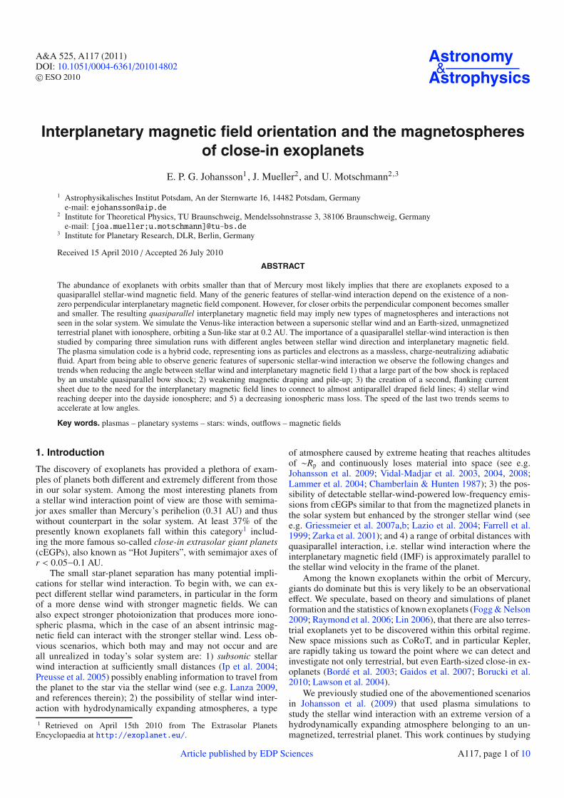
A&A 525, A117 (2011)

vB

vsw,eff

planet

Fig. 1. Illustration of how the direction of the IMF and the effectivestellar change with distance from the star. uplanet (brown) is the orbitalvelocity of the planet, usw,eff (red) is the effective stellar wind direction inthe frame of a planet in circular orbit and B (blue) is the IMF direction.The blue spiral lines represent Parker spirals (magnetic field lines). Thedepicted planet is in an orbit where effective stellar wind and magneticfield are parallel.

quasiparallel stellar-wind interaction with a Venus-likeexoplanet using simulations. Both Johansson et al. (2009) andthis work make use of hybrid simulations, a plasma simula-tion model that describes ions as particles and electrons asa massless, charge-neutralizing adiabatic fluid. Compared topure fluid models, e.g., magnetohydrodynamics (MHD), thishas the advantage of being able to handle non-Maxwellian iondistributions and resolve kinetic effects, e.g. pick-up.

2. Quasiparallel stellar wind interaction

To understand why we should expect quasiparallel interaction,we must first consider the geometry of the IMF in the solar sys-tem and which we assume is duplicated in other star systems. Inshort, magnetic field lines are frozen into the stellar wind and arethus carried away from the star in the radial direction. However,the bases of the very same field lines are frozen into the starand therefore follow its rotation. This configuration leads to themagnetic field lines in the ecliptic plane forming approximateArchimedean spirals, or Parker spirals. A consequence of thisshape is a magnetic field that is azimuthal far away from the star(e.g. at Pluto in the solar system) and becomes radial at smallerdistances2. An object in circular orbit however, experiences astellar wind velocity that is radial in orbits far away from thestar but azimuthal in lower orbits, due to increasing orbital ve-locity. It follows from this that there should be a certain distancewhere an object in circular orbit with velocity vplanet should ide-ally experience an IMF that is always parallel to the stellar winddirection. This is illustrated in Fig. 1.

To approximately calculate this distance where the IMF isaligned to the stellar wind velocity we make use of the simpleobservation that a planet in such an orbit must always lie on thevery same spiral-shaped magnetic field line as the field line ro-tates around the star. Therefore the orbital period must coincidewith the stellar rotation period, i.e.,

Ω�r =

√GM�

r, (1)

2 This argument technically assumes that the stellar wind speed doesnot increase too rapidly with distance.

where� is the stellar angular rotation velocity, M� is the stellarmass, G is the gravitational constant, and r is the orbital distance.This can be rewritten as

r = (GM�)1/3Ω−2/3� , (2)

which for ease of use can also be rephrased as

r ≈ 0.020 ×(

M�M�

)1/3 (T�

1 day

)2/3

AU (3)

where M� is the solar mass and T� is the stellar rotation pe-riod. Using for example solar values infers r = 0.16 AU or abouthalf of Mercury’s perihelion distance of 0.31 AU. We note thatthe above expression is conveniently independent of stellar windvelocity and really only depends on the IMF being frozen-in. Itdoes not assume that the stellar wind velocity is constant overdifferent radial distances. We have of course also made use of anideal picture, neglecting time-varying stellar wind velocity, tur-bulence, shock waves etc. A planet in the orbit described aboveis thus more likely to be exposed to a stellar wind that is paral-lel in some average sense rather exactly parallel at every pointin time. This combined with the improbability of finding exo-planets in exactly these orbits is the reason why we prefer tospeak of quasiparallel stellar wind interaction rather than paral-lel interaction.

The existence of orbits with quasiparallel stellar-wind inter-action, i.e. where the IMF is approximately parallel to the stellarwind direction in the planet frame, is interesting because manyof the generic features of stellar wind interaction depend on theexistence of a perpendicular magnetic field component. Thus,planets in these orbits may display very different types of mag-netospheres from what we are used to. Maybe the most obviousexample of the dependence on a perpendicular magnetic fieldcomponent is the draping of the magnetic field but also that pick-up requires it, i.e. the removal of ionospheric ions through thestellar wind induced electric field.

The behavior of plasma shocks depends on the shock an-gle θBn, i.e. the angle between the shock surface normal and theupstream magnetic field and is, as for stellar wind interactions asa whole, classified as either quasiperpendicular or quasiparalleldepending on this angle (Baumjohann & Treumann 1996). Sincethe bow shock around a planet is a more or less parabolic surface,only parts of the shock surface can be regarded as a quasiparal-lel shock for a quasiparallel stellar wind. For the same reason,a quasiparallel shock is also often present for quasiperpendicu-lar stellar wind interactions but far out on the flanks where theyhave little impact.

Parallel and quasiparallel shocks are interesting because itcan be shown that they are not stable and do not form well-defined shock surfaces the way we are used to seeing forquasiperpendicular shocks (Treumann & Jaroschek 2008a,b).It can for example be shown that MHD shocks in theory re-duce to gasdynamic shocks while in practice they are oscilla-tory up to large distances upstream (Baumjohann & Treumann1996). Hybrid simulations have also shown this to be true forhigh Mach numbers (Burgess 1989). This is because particlesreflected from quasiparallel shocks can travel significant dis-tances upstream leading to beam instabilities and an extendedforeshock region (Treumann & Jaroschek 2008a,b). This meansthat kinetic effects are important for quasiparallel shocks and hy-brid simulations should therefore be better suited to the task thanMHD. We do not delve into the theory of quasiparallel shocksbut refer to Treumann & Jaroschek (2008a,b) for more technicaldetails.

A117, page 2 of 10

E. P. G. Johansson et al.: IMF orientation and the magnetospheres of close-in exoplanets

Although quasiparallel shocks have been thoroughly studiedwith hybrid simulations (see Filippychev 2000, and referencestherein), quasiparallel stellar wind interactions have not as onecould expect given the absence of it in the solar system. In thelight of this and the multitude of discovered exoplanets in recentyears, we choose to study quasiparallel stellar wind interactionusing a series of similarly configured hybrid simulation runs.

3. The hybrid simulation model

We used the “Adaptive Ion Kinetic Electron Fluid” (AIKEF)code for the simulation runs in this work. This code is essentiallyan improved successor of our previous hybrid simulation codeintroduced in Bagdonat & Motschmann (2002). AIKEF uses thesame physical model and numerical algorithms but has some ad-ditional features that were not used in this work. We thereforedo not describe AIKEF to any great length but instead refer toJohansson et al. (2009) and Bagdonat & Motschmann (2002)and references therein for details.

The basic purpose of the simulation code is to integrate thetime evolution of collisionless plasmas in a three-dimensionalsimulation box. A planet is placed inside the simulation box andis exposed to a moving stellar wind plasma. The presence of anionosphere is emulated by surrounding the planet with an ad-ditional thin plasma-producing layer. The simulation is then al-lowed to run until a quasistationary state has been reached.

Plasma ions are, on the one hand, modeled as kinetic super-particles, each representing the motion of a larger number ofphysical ions belonging to the same species. Electrons are, onthe other hand, modeled as a massless, charge-neutralizing adi-abatic electron fluid, hence the name “hybrid simulations”. Byassuming in particular a vanishing electron mass, quasineutral-ity, and Ampère’s law with the Darwin approximation, we candescribe the system unambiguously by the magnetic field andthe positions and velocities of the superparticles (ions). In theprocess, we obtain the following equations that can then be nu-merically integrated over time. We have the time evolution ofsuperparticles

dupdt=

qp

mp

(E + up × B

), (4)

where up, qp, and mp are the velocity, charge, and mass of su-perparticle p, E is the electric field, and B is the magnetic field.The time evolution of the magnetic field is described by

∂B∂t= ∇ × (ui × B) − ∇ ×

(j × Beni

), (5)

where ui is the total ion bulk flow velocity, j is the total current,e is the elementary charge, and ni is the total ion density. Thetwo above equations use expressions for the current

j =∇ × Bμ0

(6)

and the electric field

E = − (ui × B) +j × Beni

− ∇pe

eni, (7)

where μ0 is the vacuum permeability and pe is the total thermalelectron pressure. The parameter pe is calculated as the sum ofpartial electron pressures pe,s ∝ ni,s

2 for every ion species s,where ni,s is the corresponding ion density.

Fig. 2. Orientation of the coordinate axes relative to the stellar wind andIMF. The variables v, B, and E refer to the stellar wind velocity, IMF,and electric field respectively of the undisturbed stellar wind, i.e. beforethe stellar wind interacts with the planet. The equatorial plane refers tothe xy plane, the polar plane refers to the xz plane, and the terminatorplane refers to the yz plane.

Although the hybrid simulation paradigm is better suitedthan MHD to studying quasiparallel interaction, in particular thequasiparallel shock, it is still not perfect. Since it models elec-trons as an adiabatic fluid it cannot include any electron entropyincrease over the bow shock.

3.1. Coordinate system and naming conventions

We follow the convention that the undisturbed stellar wind al-ways travels in the positive x direction and that the undisturbedIMF always lies in the xy plane with non-negative x and y com-ponents. The convective electric field E = −usw,0×B, where usw,0is the stellar wind velocity vector, will consequently always bein the negative z direction. Since both the IMF vector and thestellar wind vector lie approximately in the ecliptic plane, whichin turn approximates the equatorial plane for most of the solarsystem planets, we refer to the xy plane as the equatorial plane,although our simulated planet does not really rotate. The northpole and south pole are then where the z axis crosses the plan-etary surface, at z = +Rp and z = −Rp, respectively. Followinga similar logic, we choose to refer to the xz plane as the polarplane and the yz plane as the terminator plane. Most of theseconventions are illustrated in Fig. 2.

4. Model parameters

We chose not to consider a perfectly parallel stellar-wind inter-action because 1) a truly parallel stellar wind interaction does notpersist for very long due to the fluctuations of the stellar wind;2) it is our experience that these simulations take a long time toreach quasistationary state; and 3) the simulated ionospheres ap-pear to have difficulties in preventing the parallel stellar windfrom penetrating. We wish to avoid this penetration because,among other things, it may lead to chemical reactions with theatmosphere that are not incorporated into the simulation model.We also do not wish to consider a single quasiparallel interac-tion in isolation but find it more useful to be able to compare itwith a perpendicular interaction. This highlights the differencesand unique features caused by the quasiparallel interaction ratherthan any peculiarities that might arise from our particular choiceof parameters. An intermediate run has also been added so thatwe can study the transition between the two better. Having this

A117, page 3 of 10

A&A 525, A117 (2011)

range of simulations also has the additional advantage that onecan more easily compare with simulations in the literature, e.g.Venus studies such as Martinecz et al. (2009) and Kallio et al.(2006).

Thus, we chose to perform three simulation runs, all of themidentical with the exception of the angle αsw,0 between the undis-turbed stellar wind velocity and the IMF. We refer to these runsas the perpendicular run (αsw,0 = 90◦), the intermediate run(αsw,0 = 30◦), and the quasiparallel run (αsw,0 = 10◦).

Using a perfectly perpendicular simulation run as a referenceis interesting not only because it is the very opposite of a parallelrun, but also because it can be shown that it should ideally havea kind of mirror symmetry with the polar plane (y = 0) as asymmetry plane, i.e. y > 0 and y < 0 are mirror images of eachother when using our simulation model. The equatorial plane(z = 0) is however not a symmetry plane but would have beenhad we used ideal or resistive MHD.

We chose to consider a Venus-like stellar wind interaction,i.e. an interaction between a supersonic stellar wind and an un-magnetized terrestrial planet with an atmosphere. Part of the rea-son for this is that we have little knowledge of the intrinsic mag-netic fields to expect and wish to avoid having stronger magneticfields since particle gyroradii and gyration times then decrease,pushing the numerical cost beyond a presently acceptable limit.For this purpose, we use an Earth-sized terrestrial exoplanet,Rp = REarth, equipped with a Venus-inspired ionosphere at anorbital distance of r = 0.2 AU from a Sun-like star as the basicscenario for our simulation runs. This distance is close to ourpreviously estimated r = 0.16 AU for a circular orbit aroundthe Sun in which one would ideally experience a parallel stellarwind.

We used a simulation box with of size 5 × 6 × 7 Rp dividedinto a grid of 104× 128× 148 approximately cube-shaped cells.The exoplanet is located −0.5 Rp in the negative z direction fromthe center of the box. An asymmetric box and the location of theplanet were chosen to help us minimize the influence of wavereflections on the outer simulation box boundaries.

The simulation runs were all performed for a simulated timetsim equivalent to an undisturbed stellar wind passing through thebox between 222 and 275 times, i.e. (tsim vsw,0)/Lx = 222−275,where vsw,0 is the stellar wind velocity and Lx is the length of thesimulation box in the x direction. These run times are in practicemuch longer than necessary to reach a quasistationary state, butare needed to obtain average values of the stellar wind lost to theplanet and the ionospheric plasma lost from the planet.

4.1. Stellar wind parameters

We estimate the velocity, density, and ion and electron tempera-ture of a hydrogen-only stellar wind at a distance of 0.2 AU froma Sun-like star by following the same procedure as in Johanssonet al. (2009). Applying a hybrid simulation code to a planet-sizedobstacle does however constrain the maximum strength of themagnetic field that it is practically possible to work with due tothe need to resolve every ion gyration into several time steps.We therefore work in a low-magnetic field limit using an IMFfield strength of 12 nT. All stellar wind parameters and resultingMach numbers are summarized in Table 1.

4.2. Ionospheric parameters

The ionosphere is modeled as an oxygen-ion-producing layerabove a certain altitude where the atmosphere can be considered

Table 1. Stellar wind parameters.

Parameter Symbol ValueVelocity vsw,0 330 km s−1

Number density nsw,0 210 cm−3

IMF/magnetic field Bsw,0 12 nTVelocity-IMF angle, perpendicular run αsw,0 90◦

intermediate run αsw,0 30◦quasiparallel run αsw,0 10◦

Ion temperature Tsw,i,0 154 500 KElectron temperature Tsw,e,0 309 000 KAlfvénic Mach number MA 18Magnetosonic Mach number Mms 3.7

collisionless. We then assume that ions that travel below this al-titude are “recombined” in the denser atmosphere below. Whathappens below this altitude is thus of no concern and we there-fore in effect allow the simulation code to use this absorbingboundary as the surface of the planet.

Mostly inspired by the upper atmosphere of Venus, we use anionospheric production rate profile based on the photoionizationof atomic oxygen, assuming that the neutral atomic oxygen hasan ordinary hydrostatic profile

nO(h) = nO, surfe−h/H , (8)

where h is the altitude above the absorbing boundary, nO, surfis the density at the absorbing boundary, H is a constant scaleheight

H =kBTO

16 mpg≈ 92.8 km = 0.015 Rp (9)

calculated using a neutral oxygen temperature TO = 1764 Kand a gravitational acceleration of g = 9.81 m s−2, kB is theBoltzmann constant and mp is the proton mass. The neutralatmospheric temperature TO is chosen to be higher than thetemperature of the upper ionosphere and exosphere of Earth,∼700−1100 K (Schunk & Nagy 2000), or the exosphere ofVenus, ∼200−1000 K (Chamberlain & Hunten 1987) since weare considering a planet at a distance of only r = 0.2 AU froma Sun-like star where more energy is available to heat the upperatmosphere. With this atmospheric profile, we justify the exis-tence of a dayside ionospheric production rate that, using stan-dard methods, takes the form of a Chapman profile given by

QO+ (h, θ) =(nO, surf e−h/H

)σiI∞ exp

(−σanO, surf H

cos θe−h/H

), (10)

where σi and σa are the photoionization and absorption cross-sections for atomic oxygen, I∞ is the photon flux, and θ is theangle of incidence of the incoming EUV radiation. We used thisprofile for 0◦ ≤ θ ≤ 87◦, i.e. most of the dayside but still avoidingthe singularities at the terminator. The cross-sections are photonflux-weighted average values from the EUVAC model (Schunk& Nagy 2000; Richards et al. 1994). The photon flux is twicethat of the EUVAC model scaled to r = 0.2 AU. The extra factorof two is, once again, to ensure that we stay in a regime wherethe ionosphere is strong enough to prevent the stellar wind frompenetrating the ionosphere. While this extra factor is arbitrary,the difference is still no greater than that between the quiet andactive Sun (Huebner et al. 1992).

We also add, somewhat arbitrarily, a small constant back-ground production rate to compensate for there being ionizationmechanisms other than photoionization and to prevent Eqs. (5)

A117, page 4 of 10

E. P. G. Johansson et al.: IMF orientation and the magnetospheres of close-in exoplanets

1e-06

0.0001

0.01

1

100

0 200 400 600 800 1000 1200 1400

1

100

10000

1e+06

1e+08 0 0.05 0.1 0.15 0.2

Pro

duct

ion

rate

, Q [c

m-3

s-1]

Neu

tral

den

sity

, [cm

-3]

z [km]

z [Rp]

nOQsubsolarQnightside

Fig. 3. Ionospheric profiles used in simulation runs. Black solid line:neutral atomic oxygen density (right-hand y scale). Blue dotted line:substellar ionospheric production rate (left-hand y scale). Red dash-dot-dotted line: nightside ionospheric production rate (left-hand y scale).

Table 2. Ionospheric parameters.

Parameter Symbol ValueInitial ion temperature Ti 3000 KInitial electron temperature Te 3000 KAbsorption cross section σa 6.55 × 10−22 m−2

Ionization cross section σi 6.51 × 10−22 m−2

Ionization rate at infinity I∞σi 6.29 × 10−6 s−1

Total production rate QO+ ,tot 2.81 × 1029 s−1

Neutral oxygen boundary density nO, surf 5.00 × 1013 m−3

Neutral oxygen temperature TO 1764 KNeutral oxygen scale height H 92.8 km

and (7) from diverging due to low nightside plasma density.After this is added, the constant background ionization rate is

QO+, background = 0.10 · QO+ (h, 30◦) . (11)

The ionospheric plasma itself is produced with initial ion andelectron temperatures Ti = Te = 3000 K similar to that of the up-per ionosphere of Venus (Schunk & Nagy 2000). All ionosphericparameter values are summarized in Table 2. In addition, Fig. 3shows the neutral profile and the substellar and nightside ion pro-duction profiles. As can be seen, the ionization profile is almostproportional to the neutral density, implying that photoabsorp-tion is in practice negligible above the absorbing boundary andthat use of a Chapman profile, Eq. (10), although correct is reallymore sophisticated than necessary.

5. Results

The results are illustrated in Figs. 4−8. Figure 4 is a three-dimensional overview of the stellar wind density that comparesthe perpendicular and the quasiparallel runs, while Figs. 5−8show miscellaneous physical quantities plotted on the cross-sections of the simulation box. Plasma loss rates are summedup in Table 3.

Figures 5−7 are organized such that the left, middle, andright columns of plots refer to the perpendicular, intermediate,and quasiparallel runs, respectively. The three plots in every rowshow the same quantity. Figure 8 only shows results for thequasiparallel run. The plots contained within each single figuredepict the same cross-section in the simulation box. Color scalesare kept the same for every physical quantity. For vector plots,the color represents the true magnitude of the three-dimensionalvector. The arrow lengths are proportional to the square root of

Table 3. Rate of ionospheric plasma being removed at the outer sim-ulation box boundaries and stellar wind plasma being removed at theplanet surface.

Ionosphere Stellar windSimulation Run (s−1) (s−1)

Perpendicular run (αsw,0 = 90◦) 1.3 × 1029 (46%) 8.1 × 1024

Intermediate run (αsw,0 = 30◦) 1.2 × 1029 (42%) 9.0 × 1024

Quasiparallel run (αsw,0 = 10◦) 9.5 × 1028 (34%) 5.8 × 1025

Notes. Percentages within brackets refer to the equivalent fraction ofthe total ionospheric production rate Qtot in Table 2. Plasma can only beremoved at the planet surface and the outer simulation box boundaries.The numbers are time averages for the quasistationary state at whichthe plasma production rate of each species equals the respective time-averaged plasma removal rates (planetary surface plus simulation boxboundaries).

the strength of the respective vector quantities projected onto thecross section. The proportionality constants are however not thesame in different plots and the arrows are therefore not directlycomparable between simulation runs. All quantities are normal-ized using the equivalent background stellar-wind values.

We begin by looking at the reference run, i.e. the perpendic-ular run. As anticipated in Sect. 4, the equatorial cross-sectionsfor the perpendicular run in Fig. 5 are all very close to being mir-ror symmetric whereas the equivalent polar plane cross-sectionsfor the same run in Fig. 6 are not.

The stellar wind density in Figs. 5g and 6g allows us toidentify all the generic features we associate with the interac-tion between supersonic stellar wind and a conducting obstacle(ionosphere) without an intrinsic magnetic field. The stellar windenters the simulation box on the negative x side and travels inthe positive x direction until it passes through the bow shock,the paraboloid surface surrounding the planet on the dayside andvisible as a sudden jump in stellar wind density by a factor ofthree. Immediately downstream of the bow shock is the mag-netosheath where the stellar wind flow is diverted around theplanet. Between the magnetosheath and the planet, we find theionospheric plasma that constitutes the true obstacle because ofits conductivity and thermal pressure, Figs. 5d and 6d. The iono-sphere is separated from the magnetosheath by the so-called ioncomposition boundary (ICB).

The basic behavior of the frozen-in magnetic field similarlyfollows the stellar wind. Although somewhat difficult to see withour color scale it is enhanced by a factor of three over the bowshock in Fig. 5a as the stellar wind is compressed by the samefactor. The comoving magnetic field lines subsequently drape theplanet as the stellar wind is diverted around it, leading to a day-side pile-up of field lines and a strongly enhanced field strength.Further downstream, this leads to the creation of two lobes withoppositely directed magnetic fields, which are also separated bya current sheet.

Having familiarized ourselves with the perpendicular run,we turn our attention to how the features described above changeas the angle αsw,0 decreases, i.e. as we go to the intermediate runand finally to the quasiparallel run. Looking at the bow shock inprimarily Figs. 5g−i, and secondarily Figs. 6g−i, we can see howa region with a very unstable and not very well-defined quasipar-allel shock moves in from the negative y boundary and wanderstoward the substellar point. This manifest quasiparallel shock re-gion is, as anticipated, far from a single point but instead corre-sponds approximately to local shock angles θBn < 15◦. This alsofits with the observation that the quasiparallel shock is visible in

A117, page 5 of 10

A&A 525, A117 (2011)

Fig. 4. Three-dimensional overviews of simu-lation results for the stellar wind density in theform of intersecting cross-sections for the per-pendicular a) and quasiparallel b) simulationrun. The density is normalized to the back-ground stellar wind density. Parts of the simu-lation box have been removed to give a cleareroverview. The x, y, and z axes are in units of Rp.

the polar plane in the quasiparallel run, Fig. 6i. The transitionfrom quasiperpendicular to quasiparallel shock is also visible inthe stellar wind velocity, Figs. 5j−l. There we can see that thestellar wind begins to decelerate up to an entire ∼Rp upstreamof the original shock surface illustrating both the extent of thequasiparallel foreshock and how the influence of the obstaclethen reaches much farther upstream than for the perpendicularrun. This extended, and “thick” quasiparallel shock region de-scribed above, effectively implies that there is no clear boundarybetween the undisturbed upstream stellar wind and the down-stream magnetosheath, which in the process has become lesshomogeneous.

The draping of the magnetic field in Figs. 5a−c and 6a−c pre-dictably becomes weaker as the perpendicular IMF componentBy = Bsw,0 sinαsw,0 decreases. Furthermore, a low αsw,0 impliesthat the draped field lines will form not just a “U” curve aroundthe planet but a kind of “S” curve since they have to connect tothe field lines of the IMF. This effect manifests itself in the equa-torial plane as the appearance of an irregularly shaped secondcurrent sheet in the intermediate and quasiparallel runs besidesthe familiar current sheet downstream of the planet separatingthe nightside magnetic lobes in all three runs.

We expect that oxygen ions that for one reason or an-other find themselves inside the stellar-wind-dominated flow onthe southern hemisphere (z < 0) are accelerated away fromthe planet by the convective electric field (Figs. 7a−c) until theuO+ × B term in the Lorentz force starts to dominate over theelectric field and diverts the ions. In an ideal, perfectly homoge-neous stellar wind, this pick-up motion results in cycloid-shapedtrajectories transporting the ions downstream. The length scalefor each cycloid in a perpendicular interaction is the ion gyrationradius

rg,O+ =16mpvsw,0

eBsw,0≈ 0.72 Rp, (12)

where vsw,0 and Bsw,0 are the undisturbed stellar wind velocityand magnetic field strength. Since rg,O+ is of the same orderas the size of the planet, this described motion should be ableto transport oxygen away in the negative z direction on similarlength scales, i.e. we should naively expect an extended and vis-ible pick-up region. Looking at the ionospheric density and ve-locity in Figs. 6d−f and 7d−f does however tell us that it is not assimple as that. We see a small population of high-speed oxygenions scattered above the south pole ionosphere and downstreamof it. This can be interpreted as the aforementioned pick-up re-gion. It is essentially absent in the perpendicular run but becomesmore and more apparent in the intermediate and quasiparallel

run, although is still weak. The selected trajectories plotted inFigs. 6d−f support the notion that ions are indeed picked up fromthe ionosphere.

The absence of (large-scale) pick-up in the perpendicularrun is explained by the asymmetric draping which has led tothe ionosphere being wrapped in a locally very strong mag-netic field as shown in Fig. 6a. The magnetic field is ∼20 timesstronger than the background magnetic field implying that thelocal gyration scale, Eq. (12), is as many times smaller or aboutrg,O+ ∼ 0.035 Rp, which is smaller than the thickness ∼0.2 Rpof the layer of locally enhanced magnetic field. This meansthat a cycloidal motion that begins within this layer will gen-erally remain within it. Since the ionospheric production rateprofile in practice decreases exponentially with a scale heightof H = 0.015 Rp, we know that almost no ionospheric produc-tion will take place outside the enhanced magnetic field, hencethere will be no significant visible cycloidal motion. This ab-sence can be compared with the clear presence of an extendedpick-up region in e.g. Boesswetter et al. (2004) or Simon et al.(2006); in both of these cases, there is a lack of the same strongand localized magnetic pile-up but also of additional “hot popu-lation” exosphere components Q ∝ ln(Rp/r) producing ions ongreater altitude scales, thus ions that are very amenable to beingpicked up. Upper atmospheres do indeed often have componentswith higher temperatures and thus greater scale heights. We havehowever chosen not to include such an extra atmospheric compo-nent to reduce the number of arbitrary parameters in our model.An additional consequence of this is the absence of mass loadingat altitudes much greater than H = 0.015 Rp � Rp.

When the angle of the stellar-wind magnetic field decreases,the local magnetic field enhancement decreases as ∼ sinαsw,0from a maximum of 28 Bsw,0 in the perpendicular run to a max-imum of 4.2 Bsw,0 in the quasiparallel run and in the process theobstacle to large-scale, cycloidal motion disappears. The truemotion associated with pick-up is also a bit more complicatedthan the ideal cycloid motion previously described since 1) thestrength of the convective electric field, E = −usw × B, thatinitially accelerates the ions depends on αsw,0; 2) the directionof the cycloid motion also depends on αsw,0 implying that theion trajectories lead not only downstream but also sideways; and3) the trajectories cannot be ideal cycloids since the enhancedmagnetic field has a strong curvature around the south pole dueto draping, although this cannot be clearly seen in the includedcross sections. Figures 8a and b clearly illustrate that picked-up ions in the quasiparallel run gyrate not only downstream aswould be expected in an ideal perpendicular situation but alsosideways. This is also likely the origin of the few particles of

A117, page 6 of 10

E. P. G. Johansson et al.: IMF orientation and the magnetospheres of close-in exoplanets

Fig. 5. Simulation results in the form of equatorial plane cross-sections for the perpendicular (left column), intermediate (middle column), andquasiparallel (right column) simulation run. The first row a−c) shows the magnetic field, the second row d−f) the ionospheric density, the thirdrow g−i) the stellar wind density, and the fourth row j−l) the stellar wind velocity. The x and y axes are in units of Rp. A selection of magneticfield lines have been added to a−c).

stray oxygen well outside the main ionosphere in the equatorialplane in Fig. 5f.

The location of the ICB and the extent of the ionosphere inthe polar plane is more difficult to explain, in particular why itconsistently runs so close to the planetary surface around thesouth pole as can be seen in Figs. 6d−f and 6g−i. Combining thiswith Fig. 8a indicates that this phenomenon is very local to the

polar cross-section. This does not however contradict the notionof pick-up, which only affects ionospheric ions that appear onthe stellar-wind-dominated side of the ICB.

Turning our attention to the densities in the equatorial plane,Figs. 5d−f and 5g−i, we can note how the ICB more or lessfollows the draped magnetic field lines in the equatorial planeand becomes less and less well-defined on the flanks as the

A117, page 7 of 10

A&A 525, A117 (2011)

Fig. 6. Simulation results in the form of polar plane cross-sections for the perpendicular (left column), intermediate (middle column), and quasi-parallel (right column) simulation run. The first row a−c) shows the magnetic field, the second row d−f) the ionospheric density, and the third rowg−i) the stellar wind density. The x and z axes are in units of Rp. A selection of ion trajectories (red) originating in the higher south pole ionosphereand projected on to the polar plane have been added to d−f). The trajectories in f) are identical to those in Fig. 8a.

weakening magnetic field becomes unable to keep the twospecies from diffusing into each other. It is difficult to discernfrom the cross-sections but still unambiguous in both the equa-torial and the polar plane that the stellar wind progressivelyreaches closer and closer to the dayside planet surface for lowervalues of αsw,0. This implies that αsw,0 may influence the ex-tent to which the stellar wind plasma is lost to the planet if any.The statistics for time-averaged plasma losses are summed upin Table 3. Although this is indeed a very small data set wenote that when αsw,0 decreases ionospheric plasma loss from theplanet also decreases, first by 8% and then by another 21%. Atthe same time, stellar wind loss to the planet increases first by11% and then by 640%. Thus, both trends seem to accelerate forlower values of αsw,0. The highest stellar wind loss to the planet,5.8 × 1025 s−1, is however still small compared to both iono-spheric losses, ∼1029 s−1, and the stellar wind flow as measured

by the flow through a planetary cross-section, nsw,0vsw,0πRp2 ∼

1028 s−1.

6. Discussion and conclusions

The existence of exoplanets with orbits smaller than that ofMercury implies that some of these are experiencing a stellarwind in which the IMF is parallel to the stellar wind direction.Since many of the generic features of stellar wind interaction de-pend on the existence of a non-zero perpendicular IMF compo-nent, one can expect these interactions to result in very differenttypes of magnetospheres. We have therefore chosen to study theimportance of quasiparallel stellar-wind interaction by using a3D plasma hybrid simulation model applied to the Venus-like in-teraction between a stellar wind and a terrestrial, unmagnetized

A117, page 8 of 10

E. P. G. Johansson et al.: IMF orientation and the magnetospheres of close-in exoplanets

Fig. 7. Simulation results in the form of polar plane cross-sections for the perpendicular (left column), intermediate (middle column), and quasi-parallel (right column) simulation run. The first row a−c) shows the electric field and the second row d−f) the stellar wind velocity. The x and zaxes are in units of Rp.

Fig. 8. Simulation results in the form of termi-nator cross-sections for the quasiparallel run.Figure a) (left) is the ionospheric density andb) (right) is the ionospheric velocity. The y andz axes are in units of Rp. A selection of ion tra-jectories (red) originating in the higher southpole ionosphere and projected on to the termi-nator plane have been added to a). The sametrajectories have been added to Fig. 6f.

Earth-sized planet equipped with an ionosphere and orbiting aSun-like star at 0.2 AU. We have then compared three simula-tion runs, all identical with the exception of the angle betweenIMF and stellar wind velocity.

As expected, we have observed several significant quantita-tive and qualitative variations by changing the IMF-stellar windangle from 90◦ to 30◦, and finally to 10◦. The main changes weobserve are that 1) a large part of the substellar bow shock isreplaced by a vaguely defined and unstable quasiparallel shock;2) magnetic draping and pile-up are greatly weakened; 3) a sec-ond, very irregular current sheet is created next to the planetdue to the need for the IMF field lines to connect with themagnetic lobe antiparallel to the IMF; 4) the pick-up increasesdue to weakening (asymmetric) magnetic pile-up; 5) daysideICB moves closer to the absorbing planet surface; and 6) less

ionospheric plasma is lost from the planet and more stellar windis lost to the planet.

It is difficult to argue against all of 1)−3) being present insome form for (supersonic) quasiparallel stellar wind interac-tions with conducting obstacles. Not too many conclusions canbe drawn from 4), the increasing pick-up, since it should dependon our exact choice of parameters and in particular on us work-ing in a low magnetic field limit.

We briefly consider how these results can be generalized tosmaller IMF-stellar wind angles. Before doing so, it is worthpointing out that both the second current sheet and the increasingpick-up are only transitional and should for obvious reasons ul-timately disappear for a perfectly parallel interaction. The quasi-parallel bow shock should continue to move towards the sub-stellar point for decreasing angles and the magnetic draping and

A117, page 9 of 10

A&A 525, A117 (2011)

lobes should continue to weaken and disappear. The final magne-tosphere for a parallel interaction should theoretically be cylin-drically symmetric, assuming that it is always stable and lami-nar, which indicates the great differences one expects betweenour quasiparallel run and a parallel run.

The trend that the ICB and the stellar wind reaches closerand closer to the dayside absorbing planetary surface for smallerand smaller IMF-stellar wind angles is corroborated by our ex-perience from similar quasiparallel and parallel test runs not pre-sented in this work. In those runs, we have more often than notencountered the phenomenon that stellar wind reaches throughthe ionosphere and impacts the absorbing planetary surface inbulk for IMF-stellar wind angles smaller than the 10◦ in ourquasiparallel run. As previously mentioned, this effect is one ofthe reasons why we have not formally included such a simula-tion run in our study since it needs a more careful treatment ofthe chemistry between stellar wind and ionosphere, which wehave not yet modeled.

This relates to the observation that the amount of stellar windbeing lost to the planet, Table 3, increases when the angle de-creases and that this trend seems to accelerate for low angles.Therefore, one may suspect that the amount of stellar wind be-ing absorbed by the planet or interacting with the atmosphereis even greater and more sensitive to the IMF-stellar wind an-gle at smaller angles. The more sensitive the configuration isto the exact angle, the more incorrect it is to consider in termsof an exoplanet’s average interaction over, say, an elliptical or-bit or over shifting types of stellar wind (slow/fast). Therefore,future study should if possible not only compare results for sev-eral small angles and if necessary adequately handle reactionsbetween stellar wind and atmosphere, but perhaps incorporateknowledge of the time variation in the IMF-stellar-wind angle.If one assumes this angle dependance to hold true in generalfor stellar wind interaction with unmagnetized planets with at-mospheres, then one may speculate that there might be caseswhere the increased direct interaction between stellar wind andatmosphere because of the low IMF-stellar-wind angle produceshigher amounts of energetic neutral atoms (ENAs). These ENAscould then in principle be observable in future high resolutiontransit spectra in analogy with some interpretations of the Lyαobservations of HD 209458 b (Holmström et al. 2008; Ben-Jaffel& Sona Hosseini 2010).

As mentioned, our simulations also indicate that atmosphericmass loss varies with the IMF-stellar-wind angle, especially atlow angles. We infer this directly from the counting of super-particles but in principle also indirectly, although without quan-tifying it, as a byproduct of the atmospheric ion chemistry (e.g.charge exchange, impact ionization, which are not included inour simulation model) due to stellar wind penetrating deeper intothe actual atmosphere with decreasing angle. If we also assumethis angle dependance to hold true in general, then the IMF-stellar wind angle might also be important when relating obser-vations of exoplanetary atmospheres to planet formation, shouldthe mass loss influence planetary evolution. Mass loss estimates,including considerations of influence on planetary evolution, arealready an active topic for cEGPs (see e.g. Yelle 2004; Yelleet al. 2008; Vidal-Madjar et al. 2003, 2008; Tian et al. 2005;Lecavelier des Etangs et al. 2004; Penz et al. 2008; Baraffe et al.2004; Ben-Jaffel 2007).

Acknowledgements. The authors acknowledge the fellowship of E.P.G.J. fromthe International Max Planck Research School (IMPRS) on Physical Processesin the Solar System and Beyond of the Max Planck Institute for Solar SystemResearch (MPS) and the Universities of Braunschweig and Göttingen. TheDeutsche Forschungsgemeinschaft supported the work of E.P.G.J. partly throughgrant MO539/15 and of J.M. through grant MO539/16.

References

Bagdonat, T., & Motschmann, U. 2002, J. Comp. Phys., 183, 470Baraffe, I., Selsis, F., Chabrier, G., et al. 2004, A&A, 419, L13Baumjohann, W., & Treumann, R. A. 1996, Basic space plasma physics

(London: Imperial College Press)Ben-Jaffel, L. 2007, ApJ, 671, L61Ben-Jaffel, L., & Sona Hosseini, S. 2010, ApJ, 709, 1284Boesswetter, A., Bagdonat, T., Motschmann, U., & Sauer, K. 2004, Annales

Geophysicae, 22, 4363Bordé, P., Rouan, D., & Léger, A. 2003, A&A, 405, 1137Borucki, W. J., Koch, D., Basri, G., et al. 2010, Science, 327, 977Burgess, D. 1989, Geophys. Res. Lett., 16, 345Chamberlain, J. W., & Hunten, D. M. 1987, Theory of planetary atmospheres, An

introduction to their physics andchemistry, ed. J. W. Chamberlain, & D. M.Hunten

Farrell, W. M., Desch, M. D., & Zarka, P. 1999, J. Geophys. Res., 104, 14025Filippychev, D. S. 2000, Comput. Math. Mod., 11, 15Fogg, M. J., & Nelson, R. P. 2009, A&A, 498, 575Gaidos, E., Haghighipour, N., Agol, E., et al. 2007, Science, 318, 210Griessmeier, J.-M., Preusse, S., Khodachenko, M., et al. 2007a,

Planet. Space Sci., 55, 618Griessmeier, J.-M., Zarka, P., & Spreeuw, H. 2007b, A&A, 475, 359Holmström, M., Ekenbäck, A., Selsis, F., et al. 2008, Nature, 451, 970Huebner, W. F., Keady, J. J., & Lyon, S. P. 1992, Ap&SS, 195, 1Ip, W.-H., Kopp, A., & Hu, J.-H. 2004, ApJ, 602, L53Johansson, E. P. G., Bagdonat, T., & Motschmann, U. 2009, A&A, 496, 869Kallio, E., Jarvinen, R., & Janhunen, P. 2006, Planet. Space Sci., 54, 1472Lammer, H., Selsis, F., Ribas, I., et al. 2004, in Stellar Structure and Habitable

Planet Finding, ed. F. Favata, S. Aigrain, & A. Wilson, ESA SP-538, 339Lanza, A. F. 2009, A&A, 505, 339Lawson, P. R., Unwin, S. C., & Beichman, C. A. 2004, Precursor Science for

the Terrestrial Planet Finder, Jet Propulsion Laboratory, California Instituteof Technology, JPL Publication, 04-014

Lazio, T. J. W., Farrell, W. M., Dietrick, J., et al. 2004, ApJ, 612, 511Lecavelier des Etangs, A., Vidal-Madjar, A., McConnell, J. C., & Hébrard, G.

2004, A&A, 418, L1Lin, D. N. C. 2006, Overview and prospective in theory and observation of planet

formation, ed. H. Klahr, & W. Brandner (Cambridge University Press), 256Martinecz, C., Boesswetter, A., Fraenz, M., et al. 2009, J. Geophys. Res. (Space

Phys.), 114Penz, T., Erkaev, N. V., Kulikov, Y. N., et al. 2008, Planet. Space Sci., 56, 1260Preusse, S., Kopp, A., Büchner, J., & Motschmann, U. 2005, A&A, 434, 1191Raymond, S. N., Mandell, A. M., & Sigurdsson, S. 2006, Science, 313, 1413Richards, P. G., Fennelly, J. A., & Torr, D. G. 1994, J. Geophys. Res., 99, 8981Schunk, R. W., & Nagy, A. F. 2000, Ionospheres: Physics, Plasma Physics, and

Chemistry (Cambridge University Press)Simon, S., Boesswetter, A., Bagdonat, T., Motschmann, U., & Glassmeier, K.-H.

2006, Annales Geophysicae, 24, 1113Tian, F., Toon, O. B., Pavlov, A. A., & De Sterck, H. 2005, ApJ, 621, 1049Treumann, R. A., & Jaroschek, C. H. 2008a, [arXiv:0805.2162]Treumann, R. A., & Jaroschek, C. H. 2008b, [arXiv:0805.2579]Vidal-Madjar, A., Lecavelier des Etangs, A., Désert, J.-M., et al. 2003, Nature,

422, 143Vidal-Madjar, A., Désert, J.-M., Lecavelier des Etangs, A., et al. 2004, ApJ, 604,

L69Vidal-Madjar, A., Lecavelier des Etangs, A., Désert, J., et al. 2008, ApJ, 676,

L57Yelle, R., Lammer, H., & Ip, W. 2008, Space Sci. Rev., 139, 437Yelle, R. V. 2004, Icarus, 170, 167Zarka, P., Treumann, R. A., Ryabov, B. P., & Ryabov, V. B. 2001, Ap&SS, 277,

293

A117, page 10 of 10