arX

iv:h

ep-t

h/02

1001

4v2

8 O

ct 2

002

NIKHEF/02-009

hep-th/0210014

September 2002

Orientation matters for NIMreps

N. Sousa and A.N. Schellekens⋆

NIKHEF

NIKHEF, P.O. Box 41882, 1009 DB Amsterdam, The Netherlands

Abstract

The problem of finding boundary states in CFT, often rephrased in terms of “NIM-

reps” of the fusion algebra, has a natural extension to CFT on non-orientable surfaces.

This provides extra information that turns out to be quite useful to give the proper

interpretation to a NIMrep. We illustrate this with several examples. This includes a

rather detailed discussion of the interesting case of the simple current extension of A2

level 9, which is already known to have a rich structure. This structure can be disentan-

gled completely using orientation information. In particular we find here and in other

cases examples of diagonal modular invariants that do not admit a NIMrep, suggesting

that there does not exist a corresponding CFT. We obtain the complete set of NIMreps

(plus Moebius and Klein bottle coefficients) for many exceptional modular invariants

of WZW models, and find an explanation for the occurrence of more than one NIMrep

in certain cases. We also (re)consider the underlying formalism, emphasizing the dis-

tinction between oriented and unoriented string annulus amplitudes, and the origin of

orientation-dependent degeneracy matrices in the latter.

⋆ t58@nikhef.nl

− 2 −

1. Introduction

Boundary states in conformal field theory (CFT) have been studied for at least tworather different reasons. First of all one may need these states in a particular physicalproblem in which boundaries of the Riemann surface are important, such as open string

theory or applications of statistical mechanics. But on the other hand it has also beensuggested that the mere (non)-existence of (a complete set [1] of) boundaries may tellus something about the existence of the CFT itself.

Completeness of boundaries in usually rephrased [1], [2] in terms of an equation

involving the annulus coefficients A bia , which are non-negative integers appearing in

the decomposition of the open string spectrum (more precise definitions will be givenbelow). These integer matrices must form a non-negative integer matrix representation(NIMrep) of the fusion algebra:

A bia A c

jb = N kij A c

ka (1.1)

A general solution found by Cardy [3] is to choose A equal to the fusion coefficients. Theissue of finding non-trivial NIMreps was considered shortly thereafter in [4] in the contextof RSOS models. These authors also gave some non-trivial solutions, in particular forSU(3) WZW models. The relation to completeness of boundaries was understood in [1],after which many papers appeared giving solutions in various cases with various degreesof explicitness, see e.g. [2] and [5-15].

The link of a given NIMrep to closed CFT is made by simultaneously diagonal-izing the integer matrices A in terms of irreducible representations of fusion algebraand matching the representations that appear with the C-diagonal terms in the toruspartition function matrix Zij (by “C-diagonal” we mean the coefficients Ziic).

The issue of existence of a CFT usually arises in situations where the existenceof a modular invariant partition function (MIPF) is the only hint of a possible CFT.This occurs frequently in the case of rational CFT’s, where such partition functions aredetermined by a non-negative integer matrix that commutes with the modular transfor-mation matrices, a simple algebraic problem that can be solved by a variety of methods,including brute force. It is well known that the existence of a MIPF is necessary, but notsufficient for the existence of a CFT. Unfortunately the necessary additional checks areconsiderably harder to carry out, since they involve fusing and braiding matrices thatare available in only a few cases (for recent progress and an extensive list of referencessee [16]). It has been suggested that the existence of a complete set of boundaries mightbe used as an additional consistency check. This point was in particular emphasizedrecently by Gannon [13].

The implication of this point of view is that a CFT that cannot accommodate acomplete set of boundaries is inconsistent even if one is only interested in closed Riemann

surfaces. By the same logic, a symmetric†

CFT that cannot exist on unorientable

† We mean here a CFT with a symmetric modular invariant partition function.

− 3 −

surfaces, i.e. Riemann surfaces with crosscaps, should then be inconsistent, even if one

is only interested in orientable surfaces.

The advantage of using crosscap consistency is that there is a very simple consistency

check, namely∑

m

SimKm = 0 , if i is not an Ishibashi label (1.2)

where Km are the Klein bottle coefficients, which must satisfy the conditions Km =

Zmm mod 2 and |Km| ≤ Zmm, where Zmn is the integer matrix defining the torus

partition function.

There are, however, two caveats. First of all, non-symmetric modular invariants

manifestly do not allow non-orientable surfaces, since an orientation reversal inter-

changes the left and right Hilbert spaces. Nevertheless such partition functions may

well correspond to sensible CFT’s. It is not obvious that asymmetry of the modular

invariant is the only possible obstruction to orientation reversal. In other words, there

might exist examples of symmetric CFT’s allowing boundaries but no crosscaps. Sec-

ondly, the Klein bottle sum rule (1.2) can only be used successfully with some additional

restrictions on the allowable Klein bottle coefficients, since the integrality constraints

usually allow too many solutions. These additional restrictions are unfortunately only

conjectures, and hence on less firm ground than the integrality constraints. One of them,

the “Klein bottle constraint”, that requires the signs of the non-vanishing coefficients

Ki to be preserved in fusion:

KiKjKk > 0 if N kij 6= 0 , (1.3)

is known to be violated in some simple current examples [17]. Therefore either there is

something wrong with those examples, or a more precise formulation of the Klein bottle

constraint is needed (we consider the latter possibility to be the most likely one). The

other restriction is the trace formula [18]

∑

a

Aiaa =

Siℓ

S0ℓY ℓ

00Kℓ , (1.4)

to which no counter examples are known, but which is still only a conjecture. In this

paper we will consider the extra information from non-orientable surfaces always in

conjunction with boundary information, and we will see that violations of (1.2) usually

give the right hint regarding the existence of boundaries and presumably the existence

of the CFT. We investigated the validity of the Klein bottle constraint as well as the

trace formula (1.4) in many examples, and found additional counter examples to the

former, but additional support for the conjecture (1.4).

− 4 −

Another way in which orientation information can be used is to search for Moebius

and Klein bottle amplitudes belonging to an already given NIMrep. This can be done

by solving a set of “polynomial equations” given in [18]. In this case only the first caveat

applies: if the polynomial equations have no solution, then either the modular invariant

is not sensible or it does not admit an orientifold. Without further information this

cannot be decided unambiguously, but the examples strongly suggest a definite answer.

The orientation information is encoded in terms of a set of integer data that extends

the notion of a NIMrep. This is most naturally done in two stages, first to an “S-

NIMrep” (symmetrized NIM-rep) and then to a “U-NIMrep” (unoriented NIMrep), by

adding Moebius and Klein bottle coefficients. A given NIMrep can admit several S-

NIMreps (or none at all), which in their turn may have any number of U-NIMreps.

For example, the charge conjugation invariant has a well-known NIMrep (the Cardy

solution), which extends to at least one U-NIMrep, but often to more than one [19]

[20], obtained using simple currents. For all simple current modifications⋆

of charge

conjugation modular invariant a class of U-NIMreps has been determined in [12] (this

includes all U-NIMreps that exist for generic simple current invariants, but there might

exist additional exceptional solutions). In [6] the U-NIMreps were presented for all

the A1 automorphism invariants, including the exceptional “E7” invariant at level 16.

Another interesting class are the diagonal invariants. A general prescription for finding

their NIMreps was given in [10]. This involves the construction of a “charge conjugation

orbifold”, which does not necessarily exist. If the orbifold CFT does exist, the NIMrep

is constructed from it using simple currents. Then, using the results of [12], one may

also construct U-NIMreps for the diagonal invariant. The charge conjugation orbifold

theory was constructed explicitly for WZW-models (recently, the NIMreps for SU(N)

diagonal invariants were obtained by different methods in [15], while the case N = 3

was already considered in [4]; these authors did not consider U-NIMreps). Finally, it is

straightforward to extend the known NIMreps for the exceptional invariants of A1 [2] to

U-NIMreps. This summarizes what is presently known about U-NIMreps.

As remarked above, the existence of (S,U)-NIMreps may be used as a guiding princi-

ple to the (non)-existence of a CFT. In [13] several examples were given of MIPF without

a corresponding NIMrep. In these examples, the MIPF is an extension of the chiral al-

gebra. It was already known on other grounds that this extension was inconsistent,

and hence the non-existence of the complete set of boundaries just gives an additional

confirmation. Here we will present some examples that are automorphism invariants, for

which no simple consistency checks are available, other than modular invariance itself.

We will find examples that do not admit a complete set of boundaries, and examples that

do not admit crosscap coefficients, even though a complete set of boundaries does exist.

Perhaps surprisingly, among the examples for which a complete set of boundaries does

not exist are diagonal invariants (i.e. the Cardy case modified by charge conjugation).

This presumably implies that the charge conjugation orbifold theory does not exist.

⋆ Note that simple currents are used in two distinct ways here: to change the Klein bottle projectionfor a given modular invariant, and to change the modular invariant itself.

− 5 −

Apart from existence of a NIMrep, one may also worry about uniqueness of a NIM-

rep. At least one example is known [4][13] where a given modular invariant appearsto have more than one NIMrep. We find many more, and show how the ambiguity is

resolved by computing in addition to the annulus coefficients also the Moebius and Kleinbottle coefficients. Multiple NIMreps can be expected if there are degeneracies in the

spectrum, i.e. if Ziic > 1 for some i. There are exceptions: if the degeneracies are dueto simple currents, or if the degeneracy is absorbed into the extended characters (rather

than leading to several Virasoro-degenerate extended characters) we see no reason toexpect multiple NIMreps.

This paper is consists of two parts: a discussion of the formalism for general modularinvariants, and a set of examples illustrating several special features. In the next chapter

we discuss the formalism, with particular emphasis on the distinction between annulifor oriented and unoriented strings. We believe this clarifies some points that have

at best remained implicit in the existing literature. This discussion is presented forthe general case, allowing for Ishibashi state multiplicities larger than 1, which usually

occur for modular invariants of extension type. Chapters 3-7 contain various classes ofexamples, illustrating in different ways what can be learned about NIM-reps by paying

attention to orientation issues. The examples in section 3 concern automorphisms ofsimple current extended WZW models. Here we discover an example of a diagonal

invariant for which no NIMrep exists. In chapter 4 we discuss this in more generality,and find some additional examples of this kind. In section 5 we consider automorphisms

of c = 1 orbifolds. Since our results suggest that not all the allowed automorphisms of

extended WZW-models yield sensible CFT’s, it is natural to inspect also pure WZWautomorphisms. These were completely enumerated in [21]. We examine some of these

MIPF’s in section 6, and we find no inconsistencies. Finally in section 7 we considerexceptional extensions of WZW models, including cases with multiplicities larger than

1 and extensions by higher spin (i.e. higher than 1) currents. The results for the spin1 extensions can be understood remarkably well from the point of view of the extended

theory, whereas the results for higher spin extensions confirm the consistency of the newCFT’s obtained after the extension.

We will not present the explicit NIMreps here in order to save space, but all dataare available from the authors on request. The examples where obtained by solving

(1.1) on a computer, using the fact that all matrix elements are bounded from above byquantum dimension [13]. Apart from (1.1) we also imposed the condition that the matrix

representation should be diagonalizable in terms of the correct one-dimensional fusionrepresentations, with multiplicity Ziic . Although this is a finite search in principle, in

practice a straightforward search is impossible in essentially all cases. However, using avariety of methods – which will not be explained here – we were able to do an exhaustive

search in most cases of interest.

− 6 −

2. Orientation issues for NIM-reps

Here want to discuss two issues that have remained unsatisfactory in the literature

so far:

— Two different expressions for “annulus coefficients” are in use, one of the form

“SBB∗” and the other form “SBB”

— For a given CFT there are sometimes several choices for the complete set of bound-ary coefficients.

Here “S” stands for the modular transformation matrix and “B” for the boundarycoefficients (for reasons explained later we use the notation B instead of B here). The

indices of these quantities are as follows. A complete basis for the boundaries in a CFTare the Ishibashi states, labelled by a pair of chiral representations (i, ic). The MIPF

determines how often each Ishibashi state actually appears in a CFT. The completenesshypothesis (recently proved in [16]) states that the number of boundaries is equal to

the number of Ishibashi states. Given a MIPF, parametrized by a non-negative integralmatrix Zij , the number of boundaries should thus be given by

∑

i Ziic . Since an Ishibashi

state may appear more than once we need an additional degeneracy label α, so that therelevant Ishibashi labels are (i, α), α = 1, . . . , Ziic . We denote the Ishibashi states as

|i, α〉〉. The coupling of such a state to boundary a is given by a boundary coefficientB(i,α)a, and the completeness condition states that this should be a square, invertible

matrix. The boundary coefficients appear in the expansion of boundary states in terms

of Ishibashi states, |Ba〉〉 =∑

i,α B(i,α)a|i, α〉〉Regarding the first point above, some authors do seem to understand that the ex-

pression SBB∗ is to be used for oriented strings, and SBB for unoriented ones, but this

is rarely stated, and these expressions are often presented without justification. The for-mer expression is the one obtained most straightforwardly. The usual derivation of the

open string partition function is to transform to the closed string channel, where the am-plitude can be written as a closed string exchange between two branes. This amplitude

can be evaluated easily in the transverse (closed string tree) channel by taking matrixelements of the closed string propagator U between boundary states: 〈〈Bb|U |Ba〉〉. This

describes closed strings propagating from boundary a to boundary b. Transforming thisexpression back to the open string loop channel results in the following expression for

the annulus coefficients

A bia =

∑

j

∑

α

SijB(j,α)aB∗(j,α)b (2.1)

In general the resulting expression is not symmetric in the two indices a and b, indicat-

ing that this amplitude describes oriented strings. Obviously a symmetric expressionis obtained by dropping the complex conjugation, but that step would require some

justification.

Regarding the second point, the paradox is that on general grounds one would expect

there to exist a unique set of boundary coefficients B, given the CFT and the MIPF.

− 7 −

This is because they are the complete set of irreducible (and hence one-dimensional)representations of a “classifying algebra” [7][1] [22]. This is an abelian algebra of the

form⋆

B(i,α)aB(j,β)a =∑

k,γ

X(k,γ)

(i,α)(j,β)S0aB(k,γ)a (2.2)

whose coefficients X can be expressed in terms of CFT data like OPE coefficients andfusing matrices. Although these coefficients are rarely available in explicit form, they

are completely fixed by the algebra. Nevertheless it was found that in many cases –where (2.2) is not available and only integrality conditions were solved – a given bulk

CFT may have more than one set of boundary coefficients B, giving rise to differentannulus coefficients when the form SBB is used. In all these cases, the different annuliare related to each other by changing the coefficients B(i,α)a by a (i, α)-dependent phase.

This changes the annulus coefficients in the SBB form, but it does not change the SBB∗

annuli. Obviously such phases do not respect the classifying algebra,†

and hence at mostone of the different sets B can be equal to the unique solution B to (2.2). We use the

symbol B to denote the solution to (2.2), and B to denote any complete set of boundarycoefficients that satisfy the annulus integrality conditions. In principle, one can compute

orientable annuli (NIMreps) A bia for each choice of B, and yet another one by replacing

B by the solution B of (2.2). If indeed the coefficients B and B differ only by phases(or unitary matrices) on the degeneracy spaces, all these NIMreps are identical, and we

might as well write A bia in terms of B:

A bia =

∑

j

∑

α

SijB(j,α)aB∗(j,α)b (2.3)

Recent work on orientifold planes in group manifolds provides some useful geometri-

cal insight into the solution of the two problems stated above. The different boundaries|Ba〉〉 correspond to D-branes at different positions. The coefficients B(j,α)a specify thecouplings of these branes to closed strings. If one adds orientifold planes, there are no

changes to the positions of the D-branes, but they are identified by the orientifold reflec-tion. Hence one would expect the couplings B(j,α)a to remain unchanged, in agreement

with the classifying algebra argument given above. Nevertheless there is an importantchange in the system: without O-planes, a stack of Na D-branes gives rise to a U(Na)

Chan-Paton gauge group. In the presence of an O-plane, self-identified branes give riseto SO or Sp groups, whereas pairwise identified branes give U groups.

In string theory, oriented open strings occur when one considers branes that are not

space-time filling in an oriented closed string theory, for example the type-II superstring.

⋆ Our normalization differs from [7], in order to obtain a simpler form for the annuli.† Alternatively, one may define orientation-dependent generalizations of the classifying algebra that

incorporate the sign changes, as was done in [18]. However, there will always be one special choicewith structure coefficients derived from the CFT data in the canonical way.

− 8 −

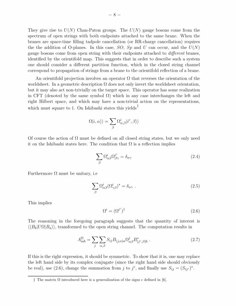
They give rise to U(N) Chan-Paton groups. The U(N) gauge bosons come from thespectrum of open strings with both endpoints attached to the same brane. When thebranes are space-time filling tadpole cancellation (or RR-charge cancellation) requires

the the addition of O-planes. In this case, SO, Sp and U can occur, and the U(N)gauge bosons come from open string with their endpoints attached to different branes,identified by the orientifold map. This suggests that in order to describe such a systemone should consider a different partition function, which in the closed string channel

correspond to propagation of strings from a brane to the orientifold reflection of a brane.

An orientifold projection involves an operator Ω that reverses the orientation of the

worldsheet. In a geometric description Ω does not only invert the worldsheet orientation,but it may also act non-trivially on the target space. This operator has some realizationin CFT (denoted by the same symbol Ω) which in any case interchanges the left andright Hilbert space, and which may have a non-trivial action on the representations,

which must square to 1. On Ishibashi states this yields‡

Ω|i, α〉〉 =∑

β

Ωiα,β |ic, β〉〉

Of course the action of Ω must be defined on all closed string states, but we only needit on the Ishibashi states here. The condition that Ω is a reflection implies

∑

β

ΩiαβΩic

βγ = δαγ (2.4)

Furthermore Ω must be unitary, i.e

∑

β

Ωiαβ(Ωi

γβ)∗ = δαγ . (2.5)

This implies

Ωi = (Ωic)† (2.6)

The reasoning in the foregoing paragraph suggests that the quantity of interest is〈〈Bb|UΩ|Ba〉〉, transformed to the open string channel. The computation results in

AΩiab =

∑

j

∑

α,β

SijB(j,α)aΩjαβB∗

(jc,β)b . (2.7)

If this is the right expression, it should be symmetric. To show that it is, one may replacethe left hand side by its complex conjugate (since the right hand side should obviously

be real), use (2.6), change the summation from j to jc, and finally use Sij = (Sijc)∗.

‡ The matrix Ω introduced here is a generalization of the signs ǫ defined in [6].

− 9 −

In order to write (2.7) in manifestly symmetric form we need a relation of the form

(B(jc,α)a)∗ =

∑

β

CjαβB(j,β),a , (2.8)

where Cj must be unitary, and is uniquely determined if we know B. Such a relationshould always hold as a consequence of CPT invariance, since it relates the emission of

a closed string state (j, jc) to the absorption of its charge conjugate. Conjugating twice

we find∑

β(Cjαβ)∗Cjc

βγ = δαγ . This relation may be used to show that

AΩiab =

∑

j

∑

α,β

SijB(j,α)a[ΩjCj ]αβB(j,β)b . (2.9)

is indeed symmetric, if AΩiab is real. The latter relation may be written as

AΩiab =

∑

j

∑

α,β

SijB(j,α)agjαβB(j,β)b . (2.10)

Conversely, if AΩiab is symmetric and B is invertible (as it is in the case of a complete

set of boundaries), then gjαβ must be symmetric. Such a “degeneracy matrix” was first

introduced in [12] for a rather different purpose, and further discussed in [18]. Here

we even encounter it in the absence of degeneracies. Note that one can of course takea square root of gj and absorb it into the definition of B(j,α)a. This the yields the

quantity previously denoted as B. This was implicitly or explicitly done in several previ-ous papers, e.g. [12] and [18], and leads to orientation-dependent boundary coefficients.

Both formalisms are of course completely equivalent if one is only interested in partitionfunctions.

Note that in most cases we do not know gj (or Ωj) and B(j,α) separately, but

we only know the integer data Ai ba or AΩ

iab. Obviously, from the former we cannotdetermine Ω, and we can only determine B(j,α) up to Ishibashi-dependent phases (or

unitary matrices in case of degeneracies). From AΩiab we can determine B(j,α) up to signs

(or orthogonal matrices in case of degeneracies), provided we know Ω. Furthermore,since the coefficients B(j,α) as well as the matrices Cj are assumed to be independent

of the orientifold choice, we can determine relative signs of two choices of Ω. In theexamples discussed so far two choices of Ω (or gj) always had relative eigenvalues ±1,

but that need not be the case in general. If one knows the classifying algebra coefficientsone can obviously determine B completely, and then also Ω and C.

The allowed choices of Ω are determined by the requirement that it must be asymmetry of the CFT. A necessary condition is that the coefficients Ωj must respect

the OPE’s of the bulk CFT, and hence presumably the fusion rules. For automorphism

− 10 −

invariants (i.e. no degeneracies) an obvious solution to that condition is Ωj = 1, but there

might be further constraints in the full CFT. Obviously these matrices will have to satisfythe appropriate generalization (to allow for degeneracies) of the crosscap constraint of[23] and [6], but we will not pursue that here, because we are only considering constraints

that do not require knowledge of fusing matrices and OPE coefficients.

A related issue is that of boundary conjugation. The boundary conjugation matrixis defined as

CBab = AΩ

0ab .

The matrix AΩ0ab must be an involution in order to get meaningful Chan-Paton groups

in string theory. Since it is an involution, we can define ac as the boundary conjugate

to a, satisfying CBaac = 1. The boundary conjugation matrix may be used to raise and

lower indices. Then we may define

AΩ bia =

∑

c

AΩiacA

Ω0cb (2.11)

For a complete set of boundaries this quantity satisfies eqn (1.1). If the latter have a

unique solution (for a given set of Ishibashi states), it follows that all quantities AΩ bia are

identical. Conversely, one can say that all quantities AΩiab are different symmetrizations

of A bia . We will refer to such a symmetrization as an S-NIMrep.

Given a NIMrep, one can always write the oriented annulus coefficient A bia in the

form (2.3), since this just amounts to diagonalizing a set of commuting normal⋆

matrices

[14]. We will now show that given an S-NIMrep, one can write AΩiac in the form (2.10).

Note that†

AΩiab = A bc

ia = AΩiba = A ac

ib

so that

A bc

iac = AΩibac = A a

ib .

Contracting this with a matrix Sim we get

∑

α

B(m,α)ac(B(m,α)bc)∗ =∑

α

B(m,α)b(B(m,α)a)∗ ,

where B(m,α)a are the set of matrices in terms of which (2.3) holds. Completeness implies

⋆ A normal matrix is a square matrix that commutes with its adjoint. This is automatically trueif A b

ia = A aicb and A b

ia is real, properties that should be treated as part of the definition of aNIMrep. It is not hard to show that the matrices AΩ b

ia satisfy this.† We are assuming here for simplicity that the NIMrep A

Ω bc

ia is unique, so we may drop thesuperscript Ω. If it is not unique, not only A

bc

ia but also B get an additional label Ω, but the restof the discussion is unaffected.

− 11 −

that the matrix B(m,α)ac has a right inverse X,

∑

a

B(m,α)acXac(n,γ) = δmnδαγ .

This leads to the following expression

∑

α

δmnδαγ(B(m,α)bc)∗ =∑

α

B(m,α)b

∑

a

(B(m,α)a)∗Xac(n,γ) .

which implies

(B(m,γ)bc)∗ =∑

α

B(m,α)b

∑

a

(B(m,α)a)∗Xac(m,γ)

=∑

α

B(m,α)bVmαγ .

Iterating this we see that V m must be a unitary matrix. Hence we get the desired

answer,

AΩiab =

∑

SimB(m,α)a)VmαγB(m,γ)b

Since the left hand side is symmetric, V m must be a symmetric matrix. It can be

written as ΩmCm to extract Ωm, but nothing guarantees that the resulting Ω is indeed

a symmetry. Indeed there may well exist symmetrizations that have no interpretation

in terms of orientifold maps.

We now have two ways of arriving at an S-NIMrep, a.) by computing 〈〈Bb|UΩ|Ba〉〉and transforming to the open string loop channel, and b.) by starting from the oriented

amplitude 〈〈Bb|U |Ba〉〉, and contracting it with CBab. Comparing the two expressions and

using completeness of boundaries, we arrive at the following expression for the action of

Ω on a boundary state

Ω|Ba〉〉 = CBab|Bb〉〉 . (2.12)

An S-NIMrep is only interesting as a first ingredient in a complete set of annuli,

Moebius and Klein amplitudes. We will refer to such a set of data as an U-NIMrep

(with “U” for unoriented). This problem can also be phrased (almost) entirely in terms

of integers [18]. The full set of conditions is then that the following quantities must exist

— NIMrep: a set of non-negative integer matrices A bia = A a

icb satisfying (1.1)

— S-NIMrep: In addition, an involution CBab such that Aiab ≡ A c

ia CBcb is symmetric

− 12 −

— U-NIMrep: In addition to the two foregoing requirements, a set of Moebius coeffi-cients Mia and Klein bottle coefficients Ki such that 1

2(Aiaa+Mia) and 12(Zii+Ki)

are non-negative integers, and the following polynomial equations are satisfied

∑

b

A bia Mjb =

∑

l

Y lij Mla

∑

a,b

CBabMiaMjb =

∑

l

Y lijKl .

(2.13)

The derivation of (2.13) in [18] uses the following formulas for Mℓa and Kℓ.

Kℓ =∑

m,α

SℓmΓmαgmαβΓmβ (2.14)

Mℓa =∑

m,α

PℓmΓmαgmαβB(mβ)a (2.15)

In the computation one uses the completeness relation

∑

a

S0mB(m,α)aB∗(ℓ,β)a = δmℓδαβ , (2.16)

which follows from A b0a = δb

a plus the completeness assumption that B is an invertible

matrix. In an analogous way one derives from A0ab = CBab:

∑

a,b

S0mB(m,α)aCBabB(ℓ,β)b = δmℓ(g

m)−1αβ , (2.17)

which implies

B∗(m,α)a =

∑

b,β

CBabg

mαβB(m,β)b (2.18)

The formulas for Mℓa and Kℓ follow from the closed string amplitudes 〈〈Ba|UΩ|Γ〉〉and 〈〈Γ|UΩ|Γ〉〉, rather than the corresponding expressions without Ω. Actually, this

should not matter, since we expect |Γ〉〉 to be an eigenstate of Ω: a crosscap correspondsto an orientifold plane, formed by the fixed points of Ω. This would still seem to allowtwo possibilities:

Ω|Γ〉〉 = ±|Γ〉〉 ,

but there are several reasons to believe that the + sign is the correct one. First of all

Ω acts on self-conjugate boundaries only with a + sign, which might suggest that the

− 13 −

same should be true for O-planes; secondly, if this relation holds with a − sign, one

finds MiaXi = −MiacXi (where X are the usual Moebius characters). This is obviously

inconsistent for self-conjugate boundaries, which must have a non-vanishing M0a. Hencein theories with at least one self-conjugate boundary, |Γ〉〉 must be an Ω eigenstate with

eigenvalue +1. This includes most CFT’s but leaves open the possibility of a rareexception. Finally, if different expressions were used for the annulus, Moebius and Klein

bottle amplitudes, tadpole factorization for the genus 1 open string amplitudes wouldnot work. While none of these arguments are totally convincing, it seems nevertheless

reasonable to assume that Ω|Γ〉〉 = |Γ〉〉, which implies MiaXi = MiacXi. In CFT’s withdegenerate Virasoro characters the implication for the Moebius coefficients is ambiguous,

but we can be more precise.

The relation Ω|Γ〉〉 = |Γ〉〉 implies a relation for the basis coefficients Γm,α appearingin the expansion

|Γ〉〉 =∑

m,α

Γ(m,α)|m, α〉〉 ,

namely

Γmc,β =∑

α

Γm,αΩmαβ (2.19)

Furthermore we will assume that the coefficients Γ satisfy the same CPT relation (2.8)as the coefficients B, i.e.

(Γ(jc,α))∗ =

∑

β

CjαβΓ(j,β) , (2.20)

which is plausible since the action is entirely on the space of Ishibashi states. Then wecan derive

Mℓcac =∑

m,α

PℓcmΓm,αgmαβB(mβ)ac

=∑

m,α,β,γ

PℓmCmc

αβ Γm,γΩmγβB(mα)a

=∑

m,α,β,γ

PℓmΓm,γΩmγβCm

βαB(mα)a = Mℓa

(2.21)

where we used (2.18), reality of Mℓ,a, (2.20), (2.19) and finally the relation Cmc

= (Cm)T

derived just after (2.8). This relation is an additional constraint that must hold if Ωis actually a symmetry. In the next chapter we will encounter solutions to (2.13) that

violates this constraint, and must therefore be rejected.

On might think that the polynomial equations (2.13) are not sufficient, just as the

NIMrep condition (1.1) is not sufficient to relate a NIMrep to a modular invariant.We must also require that in the loop channel only valid Ishibashi states propagate. In

other words, the proper channel transformation applied to the Moebius and Klein bottle

− 14 −

coefficients that solve these equations should give zero on non-Ishibashi labels. In fact,more is required: a set of boundary coefficients B(i,α)a and crosscap coefficients Γ(i,α)

that reproduce the integers. We will now show that this already follows from (2.13), i.e.

that (2.15) and (2.14) not only imply (2.13), but that the converse is also true.

Suppose the set of integers Mia satisfies the first equation. We can always writethem as Mia =

∑

m PimXma since P is invertible. Plugging this into the first equationand using (2.3), plus several inversions of P and S we get

Xℓa =∑

α

B(ℓ,α)a

[

∑

b

B(ℓ,α)bXℓb

]

≡∑

α

B(ℓ,α)aC(ℓ,α) . (2.22)

Substituting the resulting expression for Mia into the second equation we find that anyset of Klein bottle coefficients satisfying it must be of the form

Ki =∑

m,α,β

SimCm,α(gm)−1αβCm,β , (2.23)

where we used (2.17). Defining Cm,α =∑

β gαβΓm,β then gives us both Ki and Mia in

the required form. Note that (2.22) does not determine the crosscap coefficients outsidethe space spanned by the Ishibashi states. However, (2.23) shows that there is no roomfor additional components, so that Cm,α must vanish on non-Ishibashi labels. Hence nofurther conditions are required.

Note that in both cases there are far more equations than variables. In practice

the first set usually reduces to a number of independent equations slightly smaller thanthe number of Moebius coefficients (or equal, in which case the only solution is Mia =Ki = 0). Since the equations are homogeneous, the open string integrality conditionsare needed to cut the space of solutions down to a finite set. The second set of equationsproduces a unique set of coefficients Kℓ for any solution of the first. These coefficientsare then subject to the closed sector integrality conditions.

One may expect the symmetry Ω to be closely related to the choice of Klein bottleprojection Ki, which determines the projection in the closed string sector. The linkbetween the two is provided by a relation postulated in [18]:

∑

a,αβ

S0jB(j,α)agjαβB(j,β)a = Y j

00Kj , (2.24)

conjectured to hold without summation on j. Here we restored the dependence on g,that was absorbed into the definition of B in [18]. Even though we do not know gj

itself, it is clear that if this relation holds, and if we limit ourselves to automorphism

invariants and to real CFT’s,⋆

any sign change of Ωj implies a sign change of Kj for the

same value of j. However, this does not necessarily imply that Ωi is equal to Ki.

⋆ Note that Yj00

is equal to the Frobenius-Schur indicator [24][20], which vanishes for complex fields.

− 15 −

A closely related issue is the so-called “Klein bottle constraint”. This condition

would imply that the signs of the Klein bottle are preserved by the fusion rules. This

is obviously true if Ωi = Ki, since Ω is a symmetry. However, there are cases where

the Klein bottle constraint is violated in otherwise consistent simple current U-NIMreps

[17]. In those examples either Ωi 6= Ki, or Ω is not a symmetry. Since we cannot

determine Ω without further information, as discussed earlier, this cannot be decided

at present. One important check can be made, however. The examples admit (at least)

two choices for Ki, both violating the Klein bottle constraint. The sign flips relating

these choices imply, via (2.24), corresponding sign flips in Ωi, which must themselves

respect the fusion rules if each choice of Ωi does. We have checked that this is indeed

true.

3. Examples I: Automorphisms of Extended WZW models

In the following chapters we consider a variety of modular invariant partition func-

tions of CFT’s, for which we compute all the NIMreps that satisfy Ai ba = Aic a

b , all the

symmetrizations of each NIMrep, and all the Moebius and Klein bottle coefficients that

satisfy the polynomial equations (2.13), together with the usual mod-2 conditions.

Additional constraints that may be imposed are

1. The Klein bottle constraint (1.3).

2. The orientifold condition (2.21).

3. The trace formula (1.4).

4. Positivity of the Klein bottle coefficient of the vacuum.

5. Reality of the crosscap coefficients.†

We have seen examples violating any of these conditions, but Nr. 3 was only violated

if Nr. 4 (which is clearly necessary in applications to string theory) was violated as well.

In those cases it turns out that (1.4) holds with a − sign, and furthermore there was

a second solution that satisfies (1.4) and has the signs of all Klein bottle coefficients

reversed (note that the polynomial equations allow a sign flip of all Moebius coefficients,

but not in general a sign flip of all Klein bottle coefficients). We consider any violation of

conditions Nr 1,2,3 and 4 as signs of an inconsistency, but we will mention such solutions

whenever they occur.

The number of solutions we present is after removing all equivalences (i.e. the over-

all Moebius sign choice, boundary permutations that respect the NIMrep and relate

different S-NIMreps, and boundary permutations that respect an S-NIMrep and relate

different sets of Moebius coefficients).

† This is a conjecture due to A. Sagnotti.

− 16 −

The examples we consider in this chapter occur in CFT’s obtained by extendingthe chiral algebra of a WZW-model by simple currents. We emphasize that we work

in the extended CFT and hence we only consider boundaries that respect the extendedsymmetries. Nevertheless we will get information about broken boundaries from other

modular invariants of the extended theory. The cases we consider have one fixed pointrepresentation, and we apply the method of fixed point resolution of [25] to obtain themodular transformation matrix of the extended theory.

We will be interested in automorphism modular invariants of the extended theory.

Usually the fixed point resolution leads to a CFT that has one or more non-trivialfusion rule automorphisms in which the resolved fixed points are interchanged. Here we

consider three cases in which there are additional automorphisms interchanging resolvedfixed points with other representations. This phenomenon was first observed in the so-

called “E7”-type modular invariant [26] of A1 level 16 [27], which is the first in a shortseries including also A2 level 9 [28] and A4 level 5 [29].

3.1. A1 level 16

Consider first as a warm-up example A1 level 16. The extended theory has sixprimaries, which we label as (0), (1), (2), (3), (4+) and (4−), where the integers indicate

the smallest SU(2)-spin in the ground state representation. The spin 4 representation isa fixed point of the simple current, and hence is split into two degenerate representations.

In addition the representation (1) has the same conformal weight as (4+) and (4−), upto integers. All representations are self-conjugate.

This extended algebra has six modular invariants, corresponding to the six permu-

tations of (1), (4+) and (4−)

a : (0)2 + (1)2 + (2)2 + (3)2 + (4+)2 + (4−)2

c : (0)2 + (1)2 + (2)2 + (3)2 + (4+) × (4−) + (4−) × (4+)

b+ : (0)2 + (1) × (4+) + (2)2 + (3)2 + (4+) × (1) + (4−)2

b− : (0)2 + (1) × (4−) + (2)2 + (3)2 + (4−) × (1) + (4+)2

d+ : (0)2 + (1) × (4+) + (2)2 + (3)2 + (4−) × (1) + (4+) × (4−)

d− : (0)2 + (1) × (4−) + (2)2 + (3)2 + (4+) × (1) + (4−) × (4+)

When we write these partition functions in terms of SU(2) characters (which do not dis-

tinguish (4+) from (4−)) on obtains respectively the invariants of types(D, D, E, E, E, E) of A1.

The number of Ishibashi labels is 6,4,4,4,3,3 respectively, and we found preciselyone complete set of boundaries in all six cases (for the unextended theory, the NIMreps

were presented in the second paper of [2]; the U-NIMrep of the invariants “b” in theextended theory were obtained in [6].) All these sets are symmetric and have no other

symmetrizations. Furthermore in all cases except d+ and d− a U-NIMrep exists. In

− 17 −

this case we know that all these boundaries are indeed physically meaningful. The cases

(a, c), (b+, d+) and (b−, d−) are pairwise related to each other by a left conjugation (i.e.

a (4+), (4−) interchange), whereas (a, c), (b+, d−) and (b−, d+) are pairwise related by a

right conjugation. These conjugations are like T-dualities, which from the point of view

of the unextended A1 theory (the orbifold theory of this conjugation) interchange the

automorphism type of the boundary. Hence the 6 boundaries of the a-invariant plus the

4 boundaries of the c-invariant together form the 10 boundaries expected for the D-type

invariant of A1 level 16; the 4 boundaries of the d-invariant plus the 3 boundaries of the

e-invariant form the 7 boundaries of the E-type invariant of A1 level 16.

In the extended theory, orientation does not add much information, since all bound-

ary coefficients were expected to exist, and since furthermore the cases d+ and d− are

asymmetric invariants that do not admit an orientifold projection.

3.2. A2 level 9

Now consider another case with similar features, namely A2 level 9. The extended

theory now has 8 primaries, which we will label as follows

(0) : (0, 0) (1) : (0, 3) (2) : (3, 0)

(3) : (1, 1) (4) : (4, 4) (5) : (2, 2)

(6i) : (3, 3), i = 1, 2, 3

Here (a, b) are A2 Dynkin labels of one of the ground state representations. The repre-

sentations (1) and (2) are conjugate to each other, and all others are self-conjugate.

The extended theory has a total of 48 distinct modular invariants, obtained by

combining charge conjugation with the 24 permutations of (3), (61), (62) and (63).

These modular invariants are related to the following four distinct ones of A2 level 9⋆

D : [0]2 + [1][2] + [2][1] + [3]2 + [4]2 + [5]2 + 3[6]2

DC : [0]2 + [1]2 + [2]2 + [3]2 + [4]2 + [5]2 + 3[6]2

E : [0]2 + [1][2] + [2][1] + [3][6] + [6][3] + [4]2 + [5]2 + 2[6]2

EC : [0]2 + [1]2 + [2]2 + [3][6] + [6][3] + [4]2 + [5]2 + 2[6]2,

where [i], i 6= 6 stands for the full simple current orbit of the orbit representatives listed

above, and [6] is the fixed point. These modular invariants admit respectively 21, 15,

17 and 11 Ishibashi states.

⋆ Here “D” stands for “type D” as in ADE, and not for “diagonal”. Note that we have included acharge conjugation in the definitions, so that D corresponds to the C-diagonal or Cardy case, andDC to the diagonal invariant.

− 18 −

In the following table we show the number of NIMreps (of various kinds) that exist

for these 48 invariants. The results of this table are based on an exhaustive search, i.e.

the set of solutions is complete.

Nr. Permutation Proj. Ish. NIMreps S-NIMreps U-NIMreps

1 <> D 9 1 1 1

2 < a, b > D 7 0 0 0

3 < 3, b > E 7 0 0 0

4 < 1, 2 > DC 7 0 0 0

5 < 1, 2 >< a, b > DC 5 1 2 1 + 1(∗)

6 < 1, 2 >< 3, b > EC 5 1 2 1 + 1(∗)

7 < 3, a >< b, c > E 5 1 2 1

8 < 3, a, b, c > E 5 1 2 1

9 < 1, 2 >< 3, a >< b, c > EC 3 1 1 0

10 < 1, 2 >< 3, a, b, c > EC 3 1 1 0

11 < a, b, c > D 6 2(∗∗) 0 0

12 < 3, a, b > E 6 2(∗∗) 0 0

13 < 1, 2 >< a, b, c > DC 4 0 0 0

14 < 1, 2 >< 3, a, b > EC 4 0 0 0

(*) Inconsistent solution to the polynomial equations.

(**) Asymmetric NIMrep, one solution is the transpose of the other.

In this table, a, b and c denote the three resolved fixed points. The solutions are

essentially the same if a, b or c are replaced by 3, but we represent these cases separately

because they have a different interpretation. Furthermore cases 7,8 and 9,10 have pair-

wise the same solutions, because boundary CFT is only sensitive to the diagonal and

C-diagonal partition function, which is identical in these cases (note that when solving

(2.13) we do not take into account the left-right symmetry of the modular invariant). In

cases 5 and 6 the notation is as follows: the unique NIMrep allows two symmetrizations.

For each of these symmetrizations there is one set of Moebius coefficients that satisfy

the polynomial equations (2.13) (there are 40 independent equations for the 45 Moebius

coefficients). The Moebius coefficients for the second S-NIMrep (indicated with a (*)

in the table) should be rejected, however. They give rise to complex crosscap coeffi-

cients and to Klein bottle coefficients that violate the Klein bottle constraint. More

importantly, however, they violate the condition Mia = Micac , indicating that there is

no orientifold symmetry that underlies these coefficients.

− 19 −

As was the case for A1 we may expect these NIMreps to correspond to those of the

unextended theory. Furthermore the symmetry breaking boundaries may be expected

to correspond to two different modular invariants of the extended theory, obtained by

applying the cyclic permutations < a, b, c > and < a, c, b > to the “symmetric” par-

tition function. This leads to the following identifications of partition functions of the

unextended theory with triplets of extended theory partition functions

D : <>; < a, b, c >; < a, c, b >

DC : < 1, 2 >< a, b >; < 1, 2 >< b, c >; < 1, 2 >< a, c >

E : < 3, a >< b, c >; < 3, a, b >; < 3, a, c >

EC : < 1, 2 >< 3, a >; < 1, 2 >< 3, a, b, c >; < 1, 2 >< 3, a, c, b > ,

(3.1)

The first of these identifications can actually be verified, because we can compute

the NIMrep matrices for the simple current extension of A2 level 9 using the formalism

developed in [12]. Consider the matrices Ai ba , with i a zero charge primary. Since

the boundaries are in one-to-one correspondence with simple current orbits, we can

assign the corresponding charge to each boundary. As is well known [8], zero charge

boundaries are symmetry preserving, the others symmetry breaking. Now consider the

matrix elements Ai0 b0

a0, Ai0 b1

a1, Ai0 b2

a2, where the subscript on the labels denotes three

times the charge. As expected, these matrix elements are precisely given, respectively,

by the NIMreps for the modular invariants <>, < a, b, c > and < a, c, b > (we assume

that the two mutually transpose solutions in row 11 of the table are associated with the

latter two modular invariants). All other matrix elements of Ai0 vanish due to charge

conjugation. With considerably more work one should be able to compute also the

NIMreps for charged primaries. This requires extracting the boundary coefficients from

the NIMreps and in particular resolving the phase ambiguities.

The same comparison made above for the D invariant, can in principle also be made

for the other three invariants, DC, E and EC of A2 level 9. This requires an explicit

expression for the corresponding NIMreps of the unextended theory. These NIMreps

can in principle be extracted with a considerable amount of work from [4][14] (the four

cases D, DC, E and EC correspond to D(12)∗, D(12), E4(12)∗ and E5

(12) in the notation

of these authors; the remaining cases are discussed at the end of this section).

Remarkably the following four cases do not work (we list here symmetric invariants

and their cyclic permutations)

D : < 1, 2 >; < 1, 2 >< a, b, c >; < 1, 2 >< a, c, b >

This is the diagonal invariant of the extension. None of the three permutations admits

− 20 −

any NIMreps.

DC : < a, b >; < b, c >; < a, c >

Again, none of the permutations has a NIMrep.

E : < 3, a >; < 3, a, b, c >; < 3, a, c, b >

Here it seems that the two permutations of < 3, a > do admit NIMreps, but that

solution just happens to coincide with the one of < 3, a >< b, c >. Apparently thissolution should be assigned to the latter modular invariant, which is needed in (3.1).

This also explains why it exists on non-orientable surfaces, not admitted by the modularinvariant < 3, a, b, c >.

EC : < 1, 2 >< 3, a >< b, c >; < 1, 2 >< 3, a, b >; < 1, 2 >< 3, a, c >

This is precisely the opposite of the previous case: there appears to be a solution for

< 1, 2 >< 3, a >< b, c >, but it does not admit a crosscap coefficient, and should beassigned to < 1, 2 >< 3, a, b, c >, needed in (3.1). We see thus that there is precisely one

way of relating the four modular invariants of the unextended theory to groups of threemodular invariants of the extended theory, related by Z3 permutations. The solutions8 and 9 are fake ones. Removing them we get also a consistent result for the absence of

solutions for Z3-related modular invariants.

The extension to E6

There is an additional modular invariant of A2 level 9 corresponding to the conformalembedding in E6. It can be obtained by means of an exceptional extension on top ofthe simple current extension. The case has the interesting feature of allowing two (or

three) distinct NIMreps (see refs. [4][14]).

|[1] + [4]|2 + 2 × |[5]|2 (3.2)

We have analyzed this modular invariant from the point of view of the extended algebra,

and find a result that seems in agreement with [4][14]: in a complete search we did indeedfind precisely three distinct NIMreps. Each of these has 4 S-NIMreps, but only two ofthe three NIMreps allow a U-NIMrep. These two distinct U-NIMreps differ in a very

interesting way: one of them has a Klein bottle coefficient equal to 0 on the degeneratefield (i.e. the field [5]), the other has this coefficient equal to 2. The interpretation is

now immediately obvious. The extended theory, E6 level 1, is complex, and has twomodular invariants, charge conjugation and the diagonal invariant. Both invariants have

a U-NIMrep, according to refs. [3] and [10] respectively. The Klein bottle coefficientsare respectively (1, 0, 0) and (1, 1, 1). In terms of the exceptional invariant (3.2), which

cannot distinguish the complex field from its conjugate, these two cases reveal themselves

− 21 −

through a different value of the Klein bottle coefficient on the degenerate field, just as

discussed in [30]. The main novelty in this example is the fact that the two distinct

Klein bottle choices (which we knew a priori) leads to two distinct NIMreps, whereas in

all cases studied so far (i.e. the simple current extensions) different Klein bottle choices

gave rise to different unoriented annuli, but the same NIMrep.

Note that the existence of two distinct NIMreps seems to clash with the discussion

on uniqueness of the classifying algebra (and hence its representations) in chapter 2.

This example suggests a very obvious way out. Clearly the modular invariant (3.2)

belongs to two distinct CFT’s. Hence it seems plausible that after a proper resolution

of the degeneracy of the field [5] one will in fact obtain two distinct sets of classifying

algebra coefficients, although the details will have to be worked out. This phenomenon

can be expected to occur in general for modular invariants with multiplicities larger than

1, except for simple current invariants.

The two NIMreps that admit a U-NIMrep probably correspond to the cases E (12)1

and E (12)2 in [14], whereas the third NIMrep is likely to correspond to E (12)

3 , which is

discarded in [14] for not very transparent reasons.

Since the proper interpretation of these NIMreps appears to be a longstanding prob-

lem in the literature [4][14][13] we present the NIMreps here explicitly. We present them

here only in terms of the simple current extension of A2 level 9.⋆

The one with Klein bottle coefficients K0 = K4 = 1, all others zero is:

A0 =

1 0 0 0

0 1 0 0

0 0 1 0

0 0 0 1

A4 =

1 0 0 2

0 1 0 2

0 0 1 2

2 2 2 13

A5 =

0 1 1 2

1 0 1 2

1 1 0 2

2 2 2 14

Ai =

0 0 0 1

0 0 0 1

0 0 0 1

1 1 1 6

, i = 1, 2, 3, 61, 62, 63

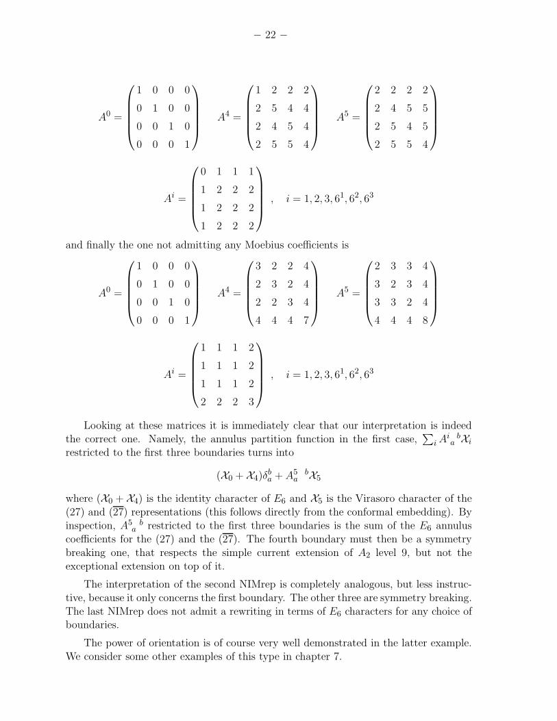
The one with Klein bottle coefficients K0 = K4 = 1, K5 = 2, all others zero is:

⋆ We have also obtained the three solutions in the unextended theory, where for this modularinvariant an exhaustive search was possible. However in the unextended theory one gets 5512 × 12 matrices, which we will not present here.

− 22 −

A0 =

1 0 0 0

0 1 0 0

0 0 1 0

0 0 0 1

A4 =

1 2 2 2

2 5 4 4

2 4 5 4

2 5 5 4

A5 =

2 2 2 2

2 4 5 5

2 5 4 5

2 5 5 4

Ai =

0 1 1 1

1 2 2 2

1 2 2 2

1 2 2 2

, i = 1, 2, 3, 61, 62, 63

and finally the one not admitting any Moebius coefficients is

A0 =

1 0 0 0

0 1 0 0

0 0 1 0

0 0 0 1

A4 =

3 2 2 4

2 3 2 4

2 2 3 4

4 4 4 7

A5 =

2 3 3 4

3 2 3 4

3 3 2 4

4 4 4 8

Ai =

1 1 1 2

1 1 1 2

1 1 1 2

2 2 2 3

, i = 1, 2, 3, 61, 62, 63

Looking at these matrices it is immediately clear that our interpretation is indeedthe correct one. Namely, the annulus partition function in the first case,

∑

i Ai ba Xi

restricted to the first three boundaries turns into

(X0 + X4)δba + A5 b

a X5

where (X0 + X4) is the identity character of E6 and X5 is the Virasoro character of the(27) and (27) representations (this follows directly from the conformal embedding). Byinspection, A5 b

a restricted to the first three boundaries is the sum of the E6 annuluscoefficients for the (27) and the (27). The fourth boundary must then be a symmetrybreaking one, that respects the simple current extension of A2 level 9, but not theexceptional extension on top of it.

The interpretation of the second NIMrep is completely analogous, but less instruc-tive, because it only concerns the first boundary. The other three are symmetry breaking.The last NIMrep does not admit a rewriting in terms of E6 characters for any choice ofboundaries.

The power of orientation is of course very well demonstrated in the latter example.We consider some other examples of this type in chapter 7.

− 23 −

3.3. A4 level 5

Consider now the simple current extension of A4 level 5. This extension has 10

representations,namely

(0) : (0, 0, 0, 0); (1) : (1, 0, 0, 1); (2) : (2, 0, 0, 2)

(3) : (0, 2, 2, 0); (4) : (0, 1, 1, 0); (5i) : (1, 1, 1, 1), i = 1, . . . , 5

All 720 permutations of the representations (1) and (5i) yield modular invariant partition

functions. In this case the table of solutions (which is complete, as in the previous case)

is as follows

Ish. NIMreps S-NIMreps U-NIMreps

10 1 1 1

8 0 0 0

7 0 0 0

6 5 (1 + 1 + 1 + 1 + 2) (0 + 0 + 0 + 0 + (0 + 2))

5 2 (1 + 1) 0

4 1 1 0

Since the six primaries (1) and (5i) are completely on equal footing as far as the

modular data (i.e. S and T ) are concerned, the solution depends only on the number of

Ishibashi states, i.e. the number of primaries not involved in a permutation. The 720

modular invariants are related to one of the following two modular invariants of A4 level

5

D : [0]2 + [1]2 + [2]2 + [3]2 + [4]2 + 5[5]2

E : [0]2 + [1][5] + [5][1] + [2]2 + [3]2 + [4]2 + 4[5]2 ,

where [0] . . . [4] denotes a complete simple current orbit. If [1] is non-trivially involved in

the permutation, the invariant of the extended theory is related to E, and otherwise to D.

The notation is as in the previous table: for example, the permutation < 1, a >< b, c >

gives rise to six Ishibashi states. We read from the table that there exist 5 NIMreps, four

of which yield one S-NIMrep, while the fifth one yields two. Of those two, one allows

no U-NIMreps, and one allows two (which are only very marginally different: the Klein

bottle coefficients are the same, but a few Moebius coefficients have opposite signs). The

five NIMreps are all completely different, and clearly not related by some unidentified

symmetry.

− 24 −

The most striking feature is again the complete absence of NIMreps for the sym-metric automorphism modular invariants < 1, a > and < a, b >, which presumably areunphysical. For the automorphism < 1, a >< b, c >< d, e > a NIMrep and even anS-NIMrep is available, but it does not allow a U-NIMrep.

As in the previous case, we can compare the NIMreps for the simple current extensionof A4 level 5 with the results from the table. This time we consider Ai0 b0

a0, Ai0 b1

a1,

Ai0 b2

a2, Ai0 b3

a3and Ai0 b4

a4, and we find that the result coincides with the NIMreps of

<> and < a, b, c, d, e > in the table. In the latter case (five Ishibashi states) we foundtwo NIMreps, which coincide respectively with the entries of the charge ±1/5 and ±2/5boundaries.

Identifying other solutions is harder than in the previous case, partly because thereis an ordering problem in determining cyclic symmetries. From the point of view ofthe fusion algebra, the five resolved fixed point representations are completely on equalfooting, so that the fusion rules are invariant under all their permutations. If we make theassumption that boundaries with broken symmetries in the unextended case correspondto boundaries for cyclically permuted modular invariants in the extended case, (as isthe case thus far), then an apparent contradiction arises. For example, the two modularinvariants < 1, 51 >< 52, 53 > and < 1, 51 >< 52, 55 >, which appear to be totallyequivalent, yield a different structure of permutations if one cyclically permutes thefixed point labels. The cyclic permutations of the symmetric modular invariants are asfollows

Nr. invariant type permutations

1 < ab > D 2 < abcd > +2 < abc >< de >

2 < 1a > E 4 < 1abcde >

3 < ab >< cd > D 4 < ab >< cd >

4 < 1a >< cd > E 2 < 1abcd > +2 < 1abc >< de >

5 < 1a >< cd > E 2 < 1abcd > +2 < 1ab >< cde >

6 < 1a >< cd >< ef > E 4 < 1ab >< de >

7 < 1a >< cd >< ef > E 2 < 1abcde > +2 < 1abc >

Here only the permutation group element is indicated. where a, b, c, d, e stand forthe fixed point fields in an unspecified order. For example < abc >< de > indicates aproduct of and order 3 and an order 2 cyclic permutation, but is not meant to imply anactual ordering of the labels. In the last four rows, the actual choice of labels in column1 determines which of the two options is valid. Note that the number of Ishibashi statesin columns 1 and 3 correctly adds up to the number of Ishibashi states of the type Dand E modular invariants (30 and 24, respectively).

Clearly, there is no NIMrep for cases 1 and 2, since there is no NIMrep for the

− 25 −

symmetric invariant. Presumably the same is true for cases 6 and 7, since there isno U-NIMreps for the symmetric invariant, which has 4 Ishibashi states. There does

exist a NIMrep in this case, but this is precisely needed for the a-symmetric invariants< 1abc >< de > and < 1ab >< cde > appearing in case 4 and 5, which is the onlyremaining chance to realize the E-invariant in terms of the extended theory.

4. Examples II: Diagonal invariants

The problems that we encountered above with the diagonal invariant of the extensionof A2 level 9 can be expected to occur quite generally for similar invariants. Consider a

CFT with a simple current of odd (and, for simplicity, prime) order N of integer spin.Suppose the unextended CFT has a complete U-NIMrep for the diagonal invariant.This assumption holds in particular for (tensor products of) WZW models, for which

the boundary states and NIMreps were constructed by means of an charge conjugationorbifold theory [10]. Although orientation issues were not discussed in that paper, theresults were obtained using a simple current extension of the orbifold theory, to which

the results of [12] apply. Those results can then be used to derive also the crosscapstates.

If a full U-NIMrep is available for the diagonal invariant, this implies that thereexists a set of Klein bottle coefficients that satisfies the following sum rule

∑

j

SijKj = 0 if i is complex

In the case of WZW models such a sum rule must in fact hold for Ki = 1 (and also forKi = νi, the Frobenius-Schur indicator), for all i. It should be possible to derive this

directly from the Kac-Peterson formula for S, but follows in any case from the argumentin the previous paragraph.

Now consider a complex representation i with vanishing simple current charge (sothat it survives in the extended theory), and whose conjugate lies on a different orbit.

Then all other representations on its orbit are necessarily complex as well, and hence

0 =∑

j

SJi,jKj =

∑

j

Sije2πiQJ (j)Kj

This implies that the sum must vanish for each value of the simple current chargeseparately, and in particular

∑

j,QJ (j)=0

Si,jKj = 0 (4.1)

This appears to be the sum rule needed for the simple current extended theory, and

indeed it is if there are no fixed points. But if there are fixed points, their total con-

− 26 −

tribution to the sum is enhanced by a factor N , so that the correct sum rule for the

extended theory does not hold.⋆

There are two ways to remedy this. One is to flip the signs of some of the Klein

bottle coefficients on the fixed points. This would violate the Klein bottle constraint,but even if one accepts that, in the examples we studied no corresponding complete setof boundaries could be found. The second solution is to modify the modular invariantin such a way that in addition to the charge conjugation, N − 1 resolved fixed points

are off-diagonal. This removes N − 1 contributions Kj for each fixed point, so thatthe sum rule holds again. Note that this also introduces new sum rules for the newoff-diagonally paired fields themselves, which are no longer Ishibashi states. The lattersum rules automatically follow from (4.1) and the general structure of the matrix S on

resolved fixed points [29]. Note, however, that for N > 3 the N−1 off-diagonal elementsneed not be paired: there are other (non-symmetric) modular invariants in which theyare off-diagonal.

The foregoing argument only shows that a plausible set of Klein bottle and crosscapcoefficients can be found if in addition to the charge conjugation one also pairs N − 1resolved fixed points off-diagonally, simultaneously for all fixed points. It also shows

that without the latter, the existence of a U-NIMrep is unlikely. A few examples of thiskind can be studied.

In the series of simple current extension of A2 level 3k the first complex theory is

A2 level 9, discussed in the previous chapter. In the next case, A2 level 12, we found aU-NIMrep for the diagonal invariant with interchange of two resolved fixed points, butno NIMrep for the diagonal invariant or interchange invariant separately (this statementis based on an exhaustive search). Extrapolating these results to levels 3 and 6 (where

the extended theory is real) one might anticipate the existence of NIMreps for the fixedpoint interchange invariants. This is indeed correct. For A2 level 3, the extension is D4

level 1, and the fixed point interchange is a simple current invariant, hence the NIMrep

is the same as the one given in [12]. Another example is the extension of E6 level 3with the spin-2 simple current. This has a novel feature in having two resolved fixedpoints, f i and gi, i = 1, 2, 3. Charge conjugation is trivial in the extended theory, andthe invariant < f1, f2 >< g1, g2 > has one NIMrep (with one S- and U-NIMrep). Note

that < f1, f2 >< g2, g3 > is not modular invariant.

Other cases with similar features occur for tensor products and coset CFT’s. Ex-amples are A2,3 × A2,3 and A2,3 × E6,3, extended with the current (J, J) and the coset

CFT A2,3 × A2,3/A2,6, where the “extension” is by the identification current. In thefirst two cases, there is no NIMrep for the diagonal invariant and one NIMrep existsfor the diagonal invariant plus fixed point interchange (yielding 4 S-NIMreps and 2 U-

NIMreps). This was demonstrated using an exhaustive search. For the coset CFT (andmany analogous ones) we expect similar results, but it was unfortunately not possibleto verify this.

⋆ It turns out the the fixed point contribution is in general non-vanishing. For simplicity we assumethat the fixed point fields themselves are real.

− 27 −

5. Examples III: c=1 orbifolds

Here we analyse some results from [11] on modular invariants of c = 1 orbifolds. In[11] we considered orbifolds at radius R2 = 2pq (p, q odd primes) (with pq+7 primaries),

and considered the automorphism that occurs [31],[21] if the radius factorizes into twoprimes.

Two cases where considered: the automorphism acting on the charge conjugationinvariant (denoted “C +A” in [11]) and acting on the diagonal invariant (denoted “D +

A”). In both cases, two U-NIMreps where found, but this was not claimed to be thecomplete set of solutions. Meanwhile we have verified that it is indeed complete in

the simplest case, pq = 15. The question whether the corresponding NIMreps are alsodistinct was not addressed in [11], but from the explicit boundary coefficients one may

verify that they are not. The solutions present some features that are worth mentioningin the present context.

In the language of the present paper the results can be described as follows

— D + A: one NIMrep, yielding 4 S-NIMreps. Of these four, three do not allow

any U-NIMreps and should presumably be viewed as unphysical. The fourth oneallows two distinct U-NIMreps, each with a different Klein bottle as described in

[11].

— C + A: one NIMrep, yielding 2 S-NIMreps. Each of these yields one U-NIMrep,

with the two Klein bottles described in [11].

Both cases contain a novelty with respect to the previous examples. In the D+A

case the two Klein bottle choices correspond to the same S-NIMrep. Hence there is nochange in the unprojected open string partition function, but some of the Moebius signs

are flipped. This means that the only difference between the two orientation choicesis the symmetrization of the representations. With both choices, the same branes are

identified, but with different signs.

In the C+A case the novelty is that the boundary coefficients of the two choices

differ by 8th roots of unity rather than fourth roots, as in all simple current cases. Thisimplies that at least one of the projections Ω has coefficients Ωj that are phases, rather

than signs. This possibility is allowed by (2.4) provided that Ωj = (Ωjc

)∗. We cannotcheck this directly because we cannot determine Ωj , but we can at least check it for the

ratio of the two different orientifold projections.

From the annuli AΩx

iab we can compute BjaΩjxCjBja, where x = 1, 2, labelling the

two cases. Since neither B nor C depended on the orientifold projection, the ratio of

these quantities for x = 1, 2 determines the ratio Ωj2/Ωj

1. We find that this ratio is ±ion the twist fields, j = σi or τi (and ±1 on all other fields), and that it does indeed

respect (2.4).

− 28 −

6. Examples IV: Pure WZW automorphisms

The automorphism modular invariants of WZW models were completely classified in

[21]. The foregoing results on automorphisms of extended WZW models may raise some

doubts about their consistency as CFT’s. We will not answer that question completely

here, but we will consider the “most exceptional” cases. The results are summarized

(together with those of the next section) in a table in the appendix.

Four basic types (which may be combined) may be distinguished: Dynkin diagram

automorphisms (i.e. charge or spinor conjugation and triality), simple current automor-

phisms, infinite series for SO(N) level 2 if N contains two or more odd prime factors,

and the three cases G2 level 4, F4 level 3 and E8 level 4. The first of these was dealt

with in [10], the second in [12], but combinations still have to be considered. For even

N , some cases follow from the results for c = 1 orbifolds, using the relation derived in

[32], but further work is needed for completing this and extending it to odd N .

This leaves the three ”doubly exceptional” cases. The first two are closely relatedsince the fusing rings are isomorphic. The NIMrep of G2 level 4 is already known, and

the one of F4 level 3 turns out to be identical. In both cases we find four S-NIMreps,

but three of them do not allow a U-NIMrep. The fourth one gives rise to one U-NIMrep.

For E8 level 4 we find one NIMrep, yielding one S-NIMrep, which in its turn gives one

U-NIMrep. The matrix elements of Rma = Bma

√Sm0 are all of the form ± 2√

17sin(2πℓ

17 ),

ℓ = 1, . . . 8, and are up to signs equal to those of the modular transformation matrix of

the twisted affine Lie algebra (denoted as in [33]) B(2)1 , level 14 or, equivalently, B

(2)7 ,

level 2, although the significance of this observation is not clear to us.

7. Examples V: WZW extensions

In the table in the appendix we list the number of (S-,U-)NIMreps some extensions of

WZW-models. In all cases the results are based on a complete search. The extensions

are either conformal embeddings (denoted as H ⊂ G, listed in [34]), simple current

extensions (denoted as “SC”), or higher spin extensions (HSE). If the CFT is complex,

there are in principle two invariants, obtained by extending the charge conjugation

invariant or the diagonal invariant. The latter possibility is indicated by a (∗) in the

first column. Most of the extensions of complex CFT’s in the table are themselves real(although some become complex after fixed point resolution). In a few cases only the

extension of the diagonal invariant was tractable, since it has fewer Ishibashi states than

the extension of the charge conjugation invariant.

We only list those simple current extensions where we found more solutions than

those obtained in [12], although we considered all accessible low-level cases in order

to check whether the set of solutions of [12] is complete. The higher spin extensions

appeared in the list of c = 24 meromorphic CFT’s [35], although some were obtained

before, or could be inferred from rank-level duality. Since the existence of these CFT’s

− 29 −

is on less firm ground than the existence of the other kinds of extensions, it is especially

interesting to find out if NIMreps exist.

In the U-NIMreps column those cases denoted with a single asterisk have Klein

bottle coefficients violating the Klein bottle constraint (but no other conditions); those

with a double asterisk violate the orientifold condition M ia = M ic

ac (and often also the

Klein bottle constraint). The ones with a triple asterisk have a value for K0 equal to −1(and hence violate the Klein bottle constraint), and they also violate the trace identity

(1.4). Often these solutions also violate the orientifold condition, and in some case they

give rise to imaginary crosscap coefficients. We will assume that the latter violations

are unacceptable, but on the other hand we will be forced to conclude that the Klein

bottle constraint violations must be accepted.

All the U-NIMreps that are listed have different Klein bottle coefficients. Those

of the spin-1 extensions can all be understood in terms of simple-current related Klein

bottle choices in the extended algebra (which is a level-1 WZW model), as described in

[12].

Some of the NIMreps in the table (in particular those for the algebras of type A)

have been discussed elsewhere (see e.g. [4] [36]), most others are new, as far as we know.

Although it is impossible to present all matrices here explicitly, they are available onrequest.

The following features are noteworthy (the characters refer to the last column)

A. In this case there are two NIMreps, one corresponding the interpretation of the

MIPF as a C-diagonal invariant of the extended algebra, and one correspondingto the diagonal interpretation.

B. In this case there are two U-NIMreps, related to the fact that the extended algebra

admits two Klein bottle choices, generated by simple currents as discussed in [20].

C. This is as case B, except that the second Klein bottle choice violates the Klein bot-

tle constraint in the unextended theory (although it does satisfy it in the extended

theory).

D. These are combinations of cases A, B and C: the modular invariant corresponds

to both diagonal and C-diagonal interpretations, each of which allows two Klein

bottle choices. Since the diagonal invariant of D2n+1 is a simple current invariant,

all four Klein bottle choices follow in fact from [12].

E. In this case the extension is by a simple current, so that [12] applies. However, that

paper contains only a single NIMrep for this case, and we find two. A plausible

explication is that the A2,3m series bifurcates for m ≥ 3 into a series of simple

current modifications of the C-diagonal and of the diagonal invariant of A2,3m.

For m < 3 these invariants coincide. The formula of [12] only applies to the firstseries, and the second solution must be interpreted as part of the other series. This

interpretation agrees with the values of the Klein bottle coefficients on the fixed

point field (resp. 3 and 1), and also with the discussion at the end of section 4.

− 30 −

F. Here the same remarks apply as in case E, but in addition the resolved fixed

points become simple currents (of SO(8) level 1), allowing an additional Kleinbottle choice (or rather three, related by triality). The three cases in the table

(not including the double asterisk ones) have Klein bottle values 3, 1 and −1 on thefixed point field. This corresponds precisely to the three values that follow from

[12] for SO(8) level 1 (for respectively the diagonal invariant, the simple currentautomorphism and the Klein bottle simple current).

G. Here “SC 2” means that the invariant is obtained using the simple current withDynkin labels J2 = (0, 2, 0). This case does not really belong in the table, because

both from the point of view of the unextended theory, A3 level 2, as in the extendedtheory, A5 level 1, the entire result can be obtained using [12]. In A3 level 2 they

follow from by combining both choices for α(J) in formula (11) of [12], appliedto the extension by J2, with the two allowed Klein bottle choices, K = 1 and

K = J . In A5 level 1 one obtains the same four Klein bottles from two distinctmodular invariants which cannot be distinguished prior to fixed point resolution.

The invariants are the diagonal one, and the one generated by the simple currentJ2 of A5. Both can be modified by the Klein bottle simple current J.

H. This is the unextended analog of the example that was explicitly presented insection (3.2.1). It is in complete agreement with the results presented there.

One can make sense of the higher spin extension results in a very similar way, becausealso in those cases we know the fusion rules of the extended algebras. In some cases

this knowledge is available via rank-level duality of the unextended algebras. Some ofthese dualities are quite clear in the table, for example C7,2 with C2,7 ≡ B2,7. In other

cases one can make use of the fact that the exceptionally extended CFT’s combine withknown CFT’s to form a meromorphic CFT, and hence must have the complex conjugate

matrix S of that CFT. For example, the E7 level 3 extension has the same fusion rulesas A5 level 1. The results for the latter CFT match those of the exceptional extension:

we find the same number of distinct U-NIMreps as in case G. The same is true, withappropriate modifications, in all other cases.

These examples demonstrate once more the importance of orientation, as well asthe completeness of the results of [12]. They also give the clearest evidence so far

that the Klein bottle constraint may well be correct in some form, but that the preciseformulation requires more work.

− 31 −

8. Conclusions

Orientation effects add useful additional structure to the a NIMreps. Furthermore,given a NIMrep, this information is relatively easy to get, and it is therefore a pity thatmany authors decide to ignore it.

Taken into account orientation leads naturally to a different formula for the annulusthan the one commonly used in the NIMrep literature. The distinctions between theexpression for oriented annuli, (2.3) and unoriented ones (2.9) are:

— The former does not depend on the choice of orientifold projection, the latter does;

— The former does not imply any boundary conjugation, the latter does.

We have given examples of modular invariants without NIMreps (including, rathersurprisingly, diagonal invariants), modular invariants with several NIMreps, NIMreps

without S-NIMreps (and hence no boundary conjugation), NIMreps with several S-NIMreps, S-NIMreps without U-NIMreps and S-NIMreps with more than one U-NIMrep,and U-NIMreps with identical Klein bottle coefficients but different Moebius coefficients.

Two distinct modular invariants may have the same Ishibashi states and hence thesame NIMreps. This happens in particular when asymmetric invariants are considered.In that case the existence of a U-NIMrep is useful information to determine whichNIMrep belongs to which modular invariant.

Although there appear to exist NIMreps that are accidental solutions to the equa-tions, and that have no physical interpretation, we have not found any U-NIMreps thatare clearly not sensible.

In all cases we know, the occurrence of multiple NIMreps for symmetric modu-lar invariants can be interpreted in a sensible way if orientation information is takeninto account, and if those NIMreps that lack a corresponding U-NIMrep are rejected.Furthermore, the occurrence of multiple U-NIMreps is in complete agreement with the

results of [12], wherever a comparison is possible. It seems plausible that only if thepartition function has multiplicities larger than 1, there can be more than one “sensible”NIMrep.

The results in section 7 (including a large set of cases not appearing in the tablebecause they agree with expectations) suggest that the results of [12] are in fact generi-cally complete, i.e. no other boundary and crosscap states can be written down that arevalid for any simple current invariant. Sporadically there may be additional solutions,

but the absence of these solutions in other cases with the same simple current orbitstructure proves that they are not generic (unfortunately there is a infinity of distinctorbits structures, and hence “generic completeness” cannot be proved rigorously in thisway).

Although our results shed some light on the infamous ”Klein bottle constraint”, itsprecise formulation clearly requires further thought. The examples in the last section

show that it does not hold in its naive form, at least not for modular invariants ofextension type.

− 32 −

The purpose of the examples in this paper is only to demonstrate various features.They should be useful to avoid incorrect conjectures, but no general conclusion can be

drawn from them with confidence. Indeed, even the combined information from theexistence of a modular invariant, NIMreps, S-NIMreps and U-NIMreps is probably ulti-

mately insufficient to decide whether a given candidate CFT really exists. Fortunately,in applications to string theory we rarely need to consider such exotic cases. Simple

current invariants is all one usually needs, and for that class the solution is known.

Acknowledgements:

We would like to thank L. Huiszoon, Ya. Stanev, A. Sagnotti, C. Schweigert, and I.

Runkel for discussions. Partial checks on the results of section 3 have been done by Ya.Stanev. Special thanks to C. Schweigert and L. Huiszoon for constructive commentson the manuscript. A.N. Schellekens wishes to thank the theory group of Tor Vergata,

where part of this work was done, for hospitality and the INFN for financial support.N.Sousa wishes to thank Stichting F.O.M. and Fundacao para a Ciencia e Tecnologia

for financial support under the reference BD/13770/97.

REFERENCES

[1] G. Pradisi, A. Sagnotti and Ya.S. Stanev, Phys Lett B354 (1995) 279; Phys. Lett.B381 (1996) 97 [arXiv:hep-th/9603097].

[2] R. Behrend, P. Pearce, V. Petkova and J-B. Zuber, Phys. Lett. B 444, 163 (1998)[arXiv:hep-th/9809097]; Nucl. Phys. B 579, 707 (2000) [arXiv:hep-th/9908036].

[3] J. Cardy, Nucl. Phys. B324 (1989) 581.

[4] P. Di Francesco and J.-B Zuber, Nucl. Phys. B338 (1990) 602.

[5] G. Pradisi, A. Sagnotti and Ya.S. Stanev, Phys Lett B354 (1995) 279 [arXiv:hep-th/9503207].

[6] G. Pradisi, A. Sagnotti and Ya.S. Stanev, Phys. Lett B356 (1995) 230 [arXiv:hep-th/9506014].

[7] J. Fuchs and C. Schweigert, Phys. Lett. B 414, 251 (1997) [arXiv:hep-th/9708141].

[8] J. Fuchs and C. Schweigert, Nucl. Phys. B 568, 543 (2000) [arXiv:hep-th/9908025];Nucl. Phys. B 558, 419 (1999) [arXiv:hep-th/9902132].

[9] J. Fuchs, C. Schweigert, Phys. Lett. B490 (2000) 163, [arXiv:hep-th/0006181].

[10] L. Birke, J. Fuchs, C. Schweigert, Adv. Theor. Math. Phys. 3 (1999) 671,[arXiv:hep-th/9905038].

[11] A.N. Schellekens and N. Sousa, Int. J. Mod. Phys. A16 (2001) 3659.

[12] J. Fuchs, L. Huiszoon, B. Schellekens, C. Schweigert, J. Walcher, Phys. Lett.

B495 (2000) 427, [arXiv:hep-th/0007174].

[13] T. Gannon, Nucl. Phys. B 627, 506 (2002) [arXiv:hep-th/0106105].

− 33 −

[14] J. B. Zuber, CFT, BCFT, ADE and all that, lectures at Bariloche 2000, [arXiv:hep-th/0006151].

[15] V. B. Petkova and J. B. Zuber, “Boundary conditions in charge conjugate sl(N)WZW theories,” arXiv:hep-th/0201239.

[16] J. Fuchs, I. Runkel and C. Schweigert, [arXiv:hep-th/0204148].

[17] L. Huiszoon, B. Schellekens and N. Sousa, Nucl. Phys. B575 (2000) 401.

[18] A.N. Schellekens and Ya.S. Stanev. JHEP 0112, 012 (2001)[arXiv:hep-th/0108035].

[19] G. Pradisi, A. Sagnotti and Ya.S. Stanev, Planar duality in SU(2) WZW models,Phys. Lett. B354 (1995) 279 [arXiv:hep-th/9503207].

[20] L. Huiszoon, B. Schellekens and N. Sousa, Phys. Lett. B470 (1999) 95.

[21] T. Gannon, P. Ruelle and M. A. Walton, Commun. Math. Phys. 179, 121 (1996)[arXiv:hep-th/9503141].

[22] V. Pasquier, J. Phys. A. 20 (1987) 5707.

[23] D. Fioravanti, G. Pradisi and A. Sagnotti, Phys. Lett. B 321, 349 (1994)[arXiv:hep-th/9311183].

[24] P. Bantay, Phys. Lett B 394 (1997) 87.

[25] J. Fuchs, A. N. Schellekens and C. Schweigert, Nucl. Phys. B 473, 323 (1996)[arXiv:hep-th/9601078].

[26] A. Cappelli, C. Itzykson and J.-B. Zuber, Nucl. Phys. B280 (1987) 445; Commun.Math. Phys. 113 (1987) 1.

[27] D. Gepner, Nucl. Phys. B287 (1987) 111.

[28] G. Moore and N. Seiberg, Nucl. Phys. B313 (1988) 16.

[29] A.N. Schellekens and S. Yankielowicz, Nucl. Phys. B334 (1990) 67.

[30] L. R. Huiszoon and A. N. Schellekens, Nucl. Phys. B 584, 705 (2000) [arXiv:hep-th/0004100].

[31] J. Fuchs, A. N. Schellekens and C. Schweigert, Nucl. Phys. B 437, 667 (1995)[arXiv:hep-th/9410010].

[32] A. N. Schellekens, Int. J. Mod. Phys. A 14, 1283 (1999) [arXiv:math.qa/9806162].

[33] J. Fuchs, B. Schellekens and C. Schweigert, Commun. Math. Phys. 180, 39 (1996)[arXiv:hep-th/9506135].

[34] F. Bais and P. Bouwknegt, Nucl. Phys. B279 (1987) 561; A.N. Schellekens andN.P. Warner, Phys. Rev. D34 (1986) 3092.

[35] A.N. Schellekens, Commun. Math. Phys. 153 (1993) 159.

[36] V. B. Petkova and J. B. Zuber, Nucl. Phys. B 463, 161 (1996)[arXiv:hep-th/9510175].

− 34 −

APPENDIX

Number of NIMreps for WZW modular invariants

MIPF NIM S-NIM U-NIM remark

A1,10 ⊂ SO(5) 1 2 1+1 B

A1,16(“E7” inv.) 1 1 1

A1,28 ⊂ G2 1 1 1

A2,3 (SC/⊂ SO(8)) 2 2+3 (0+1)+(0+1+(1∗+1∗∗∗)) F

A2,5 ⊂ SU(6) 1 2 1+1∗ C

A2,6 (SC) 2 2+1 (0+1)+(1) E

A2,9 ⊂ E6 3 2+2+2 (1+0)+(1+0)+(0+0) H

A3,2 (SC 2/⊂ SU(6)) 1 4 1+1+1+1 G

A3,4 ⊂ SO(15) 1 4 0+0 +(1 + 2∗∗)+(1 + 2∗∗) B

A9,2 (HSE∗) 1 2 1 +1

B2,3 ⊂ SO(10) 2 4+4 (0+0+1+(1∗+1∗∗∗))+(0+0+1+1) D

B2,7 ⊂ SO(14) 2 4+4 (0+0+1+(1∗+1∗∗∗))+(0+0+1+1) D

B2,12 ⊂ E8 1 4 1

B12,2 (HSE) 1 2 1

C3,2 ⊂ SO(14) 2 4+4 (0+0+1 +(1∗+1∗∗∗))+(0+0+1+1) D

C3,4 ⊂ SO(21) 1 16 1+1+14×0 B

C4,3 ⊂ SO(27) 1 16 1+1+14×0 B

C7,2 (HSE) 2 4+4 (0+0+1+(1∗+1∗∗∗))+(0+0+1+1)

D7,3 (HSE∗) 2 2+2 (0+0)+(0+2)

D7,3 (HSE) 2 2+2 (0+0)+(1+1)

C10,1 (HSE) 1 2 1 +1

D9,2 (HSE) 2 2+5 (1+1)+(5× 0)

D9,2 (HSE∗) 3 4+4+4 (1+1+0+0)+(4×0)+(4×0)

G2,3 ⊂ E6 2 2+2 (0+1)+(0+1) A

G2,4 (automorphism) 1 4 1

G2,4 ⊂ SO(14) 2 4+4 (0+0+1+(1∗+1∗∗∗))+(0+0+1+1∗) D

F4,3 (automorphism) 1 4 1

F4,3 ⊂ SO(26) 2 4+4 (0+0+1+(1∗+1∗∗∗))+(0+0+1+1∗) D

E6,4 (HSE∗) 2 2+2 (0+0)+(1+1∗)

E7,3 (HSE) 2 4+4 2 × (0+0+1+1)

E8,4 (automorphism) 1 1 1