Technical Report no. 06/11 ISSN: 0107-8283

Steiner Trees for Fixed Orientation Metrics

Marcus Brazil and Martin Zachariasen

Dept. of Computer Science University of Copenhagen • Universitetsparken 1

DK-2100 Copenhagen • Denmark

Steiner Trees for Fixed Orientation Metrics ∗

M. Brazil † M. Zachariasen‡

November 10, 2006

Abstract

We consider the problem of constructing Steiner minimum trees for a

metric defined by a polygonal unit circle (corresponding to σ ≥ 2 weighted

legal orientations in the plane). A linear-time algorithm to enumerate all

angle configurations for degree three Steiner points is given. We provide a

simple proof that the angle configuration for a Steiner point extends to all

Steiner points in a full Steiner minimum tree, such that at most six orien-

tations suffice for edges in a full Steiner minimum tree. We show that the

concept of canonical forms originally introduced for the uniform orientation

metric generalises to the fixed orientation metric. Finally, we give a O(σn)time algorithm to compute a Steiner minimum tree for a given full Steiner

topology with n terminal leaves.

Keywords: Steiner tree problem, normed plane, fixed orientation metric, canoni-

cal form, fixed topology.

1 Introduction

Given a fixed set of legal orientations in the plane, we consider the problem of

constructing minimum-length interconnection networks with the restriction that

∗Partially supported by a grant from the Australia Research Council and by a grant from the

Danish Natural Science Research Council (51-00-0336).†ARC Special Research Centre for Ultra-Broadband Information Networks, Department of

Electrical and Electronic Engineering, The University of Melbourne, Victoria 3010, Australia‡Department of Computer Science, University of Copenhagen, DK-2100 Copenhagen Ø, Den-

mark

1

line segments use legal orientations only. Furthermore, we assign weights to the

legal orientations, such that the cost of a line segment is its length times its weight,

and the total cost of the network is the sum of weighted line segment costs. This

problem is equivalent to the Steiner tree problem under a metric that has a polyg-

onally bounded unit circle.

The Steiner tree problem for fixed orientation metrics has important appli-

cations in VLSI design, where millions of nets should be routed on a (small)

number of chip layers. Each layer is typically assigned a fixed orientation in or-

der to make joint routing of multiple nets feasible. Traditionally only horizontal

and vertical routing orientations have been used in chip production, but recent

advances in production and routing algorithms have made it feasible to perform

routing in more than two perpendicular orientations. The best known examples

of such recent routing paradigms are the Y-architecture [8, 9] (where three uni-

formly distributed orientations are used) and the X-architecture [18, 20] (where

four uniformly distributed orientations are used). Furthermore, there is a growing

need for assigning weights to individual layers, such that some orientations can

preferred or deferred [22].

In addition to applications in VLSI design, fixed orientation metrics can be

used to approximate arbitrary metrics in the plane. As shown is this paper, in-

creasing the number of legal orientations only increases the running times of com-

puting Steiner minimum trees (SMTs) linearly. Therefore it is feasible to make

tight approximations of arbitrary unit circles by polygonal unit circles.

Algorithms for solving several fixed orientation distance problems were pro-

posed by Widmayer et al. [19]. For the Steiner tree problem, the rectilinear case

— where two perpendicular orientations are given — has been studied most inten-

sively due to its applications in traditional VLSI design [11, 12, 13, 24]. Important

algorithms and fundamental properties for SMTs in uniform orientation metrics

were given in [1, 2, 3, 16].

The Steiner tree problem in fixed orientation metrics is NP-hard, but when the

topology of the tree is known, the problem can be solved in polynomial time by

using linear programming [21, 25]. Moreover, for the uniform orientation problem

with λ ≥ 2 orientations (and assuming that the topology is full and has n terminal

points as leaves) a O(λn) algorithm was proposed by Brazil, Thomas, Weng and

Zachariasen [5]. The concept of forbidden subpaths from [3, 4] played a crucial

role in achieving this fast algorithm.

In this paper we study the geometric structure of SMTs in order to show that

they can be constructed in linear time when the topology of the tree is known. This

is a significant generalisation of similar results for uniform orientation metrics [5].

2

The results in this paper also nicely complement similar results, such as those of

Du et al. [10], for Steiner trees in any normed space defined by a strictly convex

and differentiable unit circle.

We have endeavoured, in this paper, to find simple, direct proofs of these re-

sults. Particularly worthy of mention is Theorem 5.5, which shows that each full

and fulsome component of an SMT only requires a small number of different ori-

entations. Not only is this a key to establishing the canonical forms in the later

parts of the paper, but it also provides a much simpler alternative proof to the less

general and highly technical results on directions and forbidden subpaths in SMTs

for uniform orientation metrics in [3, 4, 5]. Our paper essentially subsumes the

main results of these papers, and many other structural results that have appeared

in the literature on uniform orientation (including rectilinear) SMTs.

We begin by generalising the concept of direction sets from [5] to fixed orien-

tation metrics and present a Θ(σ) time algorithm to enumerate all direction sets

for an arbitrary fixed orientation metric with σ ≥ 2 legal orientations. Then we

show that direction sets extend throughout full SMTs — meaning that the edges

in a full SMT use at most six legal orientations. In addition, we show that these

full SMTs can be assumed to have certain canonical forms; one of these canonical

forms has the property that the edges of a full SMT use at most four legal orienta-

tions. Furthermore, on the basis of the so-called depth-first order canonical form

we give an O(σn) time algorithm to determine a SMT for a given full Steiner

topology with n terminal leaves.

The paper is organised as follows. In Section 2 we define the Steiner tree prob-

lem in normed planes formally, present some known results and fix our notation.

In Section 3 we present a useful geometric characterisation of meeting angles for

Steiner points, and in Section 4 we introduce the concept of direction sets and

show that we can identify all direction sets in Θ(σ) time. We show that a full

SMT uses at most six legal orientations (coming from a single direction set) in

Section 5. In Section 6 we give some fundamental results on length-preserving

perturbations of Steiner points, and we introduce the concept of canonical forms

for full SMTs. Based on these canonical forms, in Section 7 we devise a linear-

time algorithm to compute a SMT for a given full Steiner topology. We conclude

the paper in Section 8.

3

a) b) d)c)

Figure 1: Examples of polygonal unit circles. a) Rectilinear (2 perpendicular

orientations). b) Uniform orientations (λ = 4). c) Non-uniform orientations (σ =3). d) General weighted non-uniform orientations.

2 Preliminaries

We begin by setting some basic definitions and notation, and establishing gener-

alisations of some important properties of SMTs for uniform orientation metrics.

For a more detailed development of these properties, see [2, 5].

2.1 Normed Planes

Given a compact, convex, centrally symmetric domain D in the Euclidean plane

E2, one can define a norm ‖ · ‖D : E2 → R+ by setting ‖x‖D = r where

x = ru and u ∈ ∂D, the boundary of D. Denote the (closed) line segment joining

distinct points x and y by xy. We can then define a metric | · |D on E2 by setting

|xy|D = ‖x−y‖D. The resulting metric space M = (E2, | · |D) is called a normed

(or Minkowski) plane with unit disc D. By definition, ∂D = {x : ‖x‖D = 1}, and

is often referred to as the unit circle.

In this paper we will limit our attention to normed planes in which the unit

circle ∂D is a centrally symmetric polygon. The best known example of this is the

rectilinear plane [11] with norm ‖(a, b)‖D = |a|+ |b|. Here ∂D is a square whose

two diagonals lie on the x-axis and y-axis respectively (Figure 1a). An important

generalisation of the rectilinear plane is the λ-geometry plane [2], for each integer

λ(≥ 2), in which ∂D is a regular 2λ-gon (Figure 1b). Further generalisation is

denoted fixed orientation geometry [19] (Figure 1c).

In the λ-geometry plane, or in any normed plane in which ∂D is a centrally

symmetric 2σ polygon inscribed in a (Euclidean) unit circle, we can avoid the dif-

ficulties of computing directly with the associated metric as follows. We assume

4

that line segments are restricted to lying in σ distinct legal orientations corre-

sponding to the σ diagonals of ∂D. Then, for any pair of distinct points x and y,

the length of the shortest path between them composed of legal line segments is

equal to |xy|D. In other words, line segments in the normed plane can be repre-

sented by minimum paths composed of legal line segments in the Euclidean plane.

See [19] for more details on the properties of such a representation. This will be

our point of view throughout this paper.

As noted in [17], this idea can be extended to normed planes in which ∂D is

any centrally symmetric 2σ polygon — not necessarily inscribed in a Euclidean

unit circle (Figure 1d). Again line segments in the normed plane can be repre-

sented by paths composed of legal line segments, but now the total length of such

a path is determined by weighting each legal line segment according to its ori-

entation. The weighting on each line segment corresponds to the inverse of the

distance of the corresponding vertex of ∂D from the centre of D. One can again

show, using similar arguments to those in [19], that the minimum length of such a

path corresponds to the normed plane distance metric between its endpoints.

It is natural to ask whether this approach can be extended to any given set

of σ orientations with given weights for each orientation. A potential problem is

that the corresponding 2σ polygon may not be convex, meaning that we do not

have a normed plane. However, we can circumvent this difficulty by considering

the convex hull of the corresponding polygonal region. For any vertex of the 2σpolygon that does not lie on this convex hull, the corresponding orientation will

never appear in a minimum path because a line segment in that orientation can

always be replaced by line segments in other legal orientations at a smaller total

cost. Hence, in this sense our approach is completely general for all finite sets of

orientations and all possible weightings.

2.2 Steiner Trees in Normed Planes with Polygonally Bounded

Unit Circle

Throughout this paper, we assume that a normed plane whose unit circle ∂D is a

centrally symmetric polygon is given. Let σ ≥ 2 denote the number of distinct

legal orientations in the normed plane.

Given a set of points N (so-called terminals) in the plane, a Steiner minimum

tree (SMT) is a shortest possible interconnection of N under the metric given by

∂D. A SMT may contain vertices of degree three or more that are not among the

given terminals; these vertices are denoted Steiner points.

5

The graph structure of a tree T (i.e., the pattern of adjacencies of the vertices

for a given labelling of the terminals) is referred to as its topology T . If, for the

given norm, the total edge length of T , |T |D, is minimum for a given topology

T (possibly in a degenerate way), then we say that T is a SMT for T . For a

fixed topology it follows that |T |D, treated as a function of the Steiner points of

T , is a convex function (since T lies in a normed plane). Note, however, that this

convexity is not strict; it may be possible to move Steiner points in a SMT without

increasing the length of the tree.

A tree T or its topology T is said to be full if all its terminals have degree 1; if

every Steiner point furthermore has degree three, then T is denoted a full Steiner

topology. Given any SMT T , we can decompose T into full components, that is,

into full SMTs that meet only at terminals. Furthermore, T or its topology T is

said to be fulsome if T contains the maximum possible number of full compo-

nents for any SMT on the terminal set of T . If we perturb the Steiner points in

a fulsome SMT (without changing the length of the tree), then we cannot make a

Steiner point coincide in position with one of the terminals. Clearly, for any set of

terminals there always exists a SMT in which every full component is fulsome.

The edges of Steiner trees will be assumed to be represented by paths com-

posed of line segments in legal orientations, as discussed in Section 2.1. It follows

from [19] that each edge (u, v) of a Steiner tree uses at most two legal orientations;

furthermore these two orientations are necessarily adjacent. When two legal ori-

entations are required to represent an edge, then we call the edge a bent edge. Bent

edges can be realised using exactly two legal line segments. There are two pos-

sible embeddings of such a path in the plane E2, as shown in Figure 2a. A point

(of degree 2) at which two legal line segments with different orientations meet is

called a corner point. There are, of course, many other possible embeddings using

multiple corner points, and the union of all these embeddings (or shortest paths)

is a parallelogram R(u, v). It is sometimes useful to consider an embedding with

two corner points (as shown in Figure 2b) which has the property that the path has

the same orientation at both endpoints.

3 Meeting Angles for Steiner Points

In this section we give a complete characterisation of the distribution of meeting

angles of Steiner points in SMTs for a metric defined by unit circle ∂D. Let ul,

l = 0, . . . , 2σ−1 be the 2σ vectors that define the vertices of the unit circle ∂D (in

counter-clockwise order around the circle). These are unit vectors in the metric

6

a) b)

u

v

R(u, v)

c2

c1

u

v

Figure 2: Embedding of a bent edge. a ) The two embeddings uc1v and uc2vthat only require two line segments (and a single corner point); the union of all

shortest paths between u and v is denoted by R(u, v). b) An embedding with

identical orientations at endpoints.

given by ∂D, that is, they have length 1 under metric |·|D. By the central symmetry

of ∂D, we have that ul = −u(l+σ) mod 2σ. Each unit vector corresponds to a legal

direction, that is, under this metric, any (oriented) legal line segment must use one

of the 2σ unit vector directions. The successor of unit vector ul is the vector ul+1

where l + 1 := (l + 1) mod 2σ, l = 0, . . . , 2σ − 1.

In the remainder of this paper will make frequent use of the assumption that

∂D is placed somewhere in the plane such that its centre coincides with a given

point s. For such a fixed centre we can unambiguously refer to the vertices of ∂D,

which are the endpoints of the unit vectors ul for this fixed centre. The vertex that

corresponds to the endpoint of unit vector ul is denoted by ul for l = 0, . . . , 2σ−1.

3.1 Steiner Configurations

Following [17], we define a Steiner configuration in the normed plane as a star

with centre s and leaves x1, . . . , xm (with s, x1, . . . , xm all distinct) that is part

of some SMT with Steiner point s. By [17], Steiner points in a normed plane

have degree at most 4, hence m = 3 or 4 in a Steiner configuration. Here we

first consider the case where m = 3, and return to the (special) m = 4 case in

Section 5.

Consider a star with Steiner point s and leaves x1, x2 and x3. Assume w.l.o.g.

that the counter-clockwise order of the leaves is x1, x2, x3. We define the meeting

angles of s to be the angles ∠x1sx2, ∠x2sx3 and ∠x3sx1, i.e., the angles that

7

x1

x3

x2

∠x1sx2

∠x3sx1∠x2sx3

s

Figure 3: Meeting angles.

appear counter-clockwise around the Steiner point s (Figure 3).

Du et al. [10] proved the following result for strictly convex and differentiable

unit circles (which includes the Euclidean metric): If one of the edges of the star,

say sx1, is given, then the orientations of the other edges sx2 and sx3 are unique.

In other words, if Steiner point s and one of the leaves, say x1, are given, then the

meeting angles of s are unique. In this section we develop an analog version of this

result for polygonal unit circles. We start with the following theorem from [14],

which holds for any normed plane.

Definition 3.1 An angle φ = ∠x1sx2 is critical if φ ≤ π and there exists a point

x3 6= s such that Steiner point s with leaves x1, x2, x3 forms a Steiner configura-

tion, with φ = ∠x1sx2 as one of the meeting angles. (Compared to the definition

of critical in [14] we have added the condition that the meeting angle is at most π.)

Theorem 3.1 [14] A star with centre s and leaves x1, x2, x3 forms a Steiner con-

figuration in a normed plane if and only if all meeting angles are critical.

Chakerian and Ghandehari [7] gave a very useful characterisation of Steiner

configurations for strictly convex and differentiable unit circles. If a unit circle is

placed with its centre at s and l1, l2 and l3 are the tangents of the unit circle where

the rays s → x1, s → x2 and s → x3 intersect the unit circle, then l1, l2 and l3form a triangle whose centroid coincides with s. We say that the tangents l1, l2 and

l3 have the centroid-property. For more general unit circles, including polygonal

unit circles, the tangents are not in general well-defined. However, by considering

supporting lines instead of tangents, the following slightly weaker result can be

proved for arbitrary normed planes (or unit circles):

8

Lemma 3.2 [14] The following statements are equivalent in a normed plane with

unit circle ∂D:

(i) ∠x1sx2 is a critical angle

(ii) if the unit circle ∂D with centre s intersects the ray s → x1 at x′

1 and the ray

s → x2 at x′

2, then there exist lines l1, l2 and l3 supporting ∂D, l1 at x′

1 and

l2 at x′

2, such that s is the centroid of the triangle formed by l1, l2 and l3 (or

equivalently, l1, l2 and l3 have the centroid-property).

3.2 Steiner Configurations for Fixed Orientation Metrics

Based on Lemma 3.2, we will give a characterisation of Steiner configurations for

polygonal unit circles that is similar to the one shown by Chakerian and Ghan-

dehari [7]. In order to do so, we need to characterise under which conditions a

given supporting line l1 of the unit circle can be a side in a triangle of supporting

lines that has s as its centroid. Our characterisation will be based on the following

condition on when set of supporting lines l1, l2 and l3 has the centroid-property.

Lemma 3.3 [10] Let l0 be the line that is parallel to l1 and contains s. Let ∆be the Euclidean distance between the parallel lines l1 and l0. Consider the line

L that is parallel to l1 at distance 3∆ from l1 (and at distance 2∆ from l0). Let

w2 be the intersection of l2 with l0 and let w3 be the intersection of l3 with l0(Figure 4a). Then supporting lines l1, l2 and l3 satisfy the centroid property if and

only if (i) lines l2 and l3 intersect somewhere on the line L, and (ii) |sw2| = |sw3|,where | · | denotes the Euclidean distance.

In the following lemmas and theorems we will frequently refer to l0 and L as

defined by Lemma 3.3.

Lemma 3.4 Let l1, l2 and l3 be a set of supporting lines that fulfils the centroid-

property, and let l0 be the line that is parallel to l1 and contains s. Then neither l2nor l3 can support ∂D at a point that is strictly between l1 and l0.

Proof. Assume that l2 supports ∂D at a point x2 that is strictly between l1 and l0(Figure 4b), and let w2 denote the intersection of l2 with l0. Consider the point

y opposite to x2 on ∂D. By the central symmetry of ∂D, there exists a line lysupporting ∂D at y which is parallel to l1 (Figure4b). Let w be the intersection of

ly with l0. Clearly we have |sw2| = |sw|.

9

a) b)

∆

2∆

l1

l0

L

l3 l2

s w2

l1

l0

ly

s w2

l2

x2

w

y

w3

Figure 4: Illustration of proof of Lemma 3.4. a) Geometric characterisation of

triangle with centroid s. b) Tangent l2 cannot be part of a triangle with centroid s.

If supporting line l3 exists, then it can be obtained by rotating ly clockwise

along the boundary of ∂D. Since each of the rotation points are strictly above l0,

the distance |sw| increases strictly as ly is rotated. Thus we have that |sw3| >|sw2|, where w3 is the intersection of l3 with l0. By Lemma 3.3, supporting lines

l1, l2 and l3 do therefore not have the centroid-property.

A similar result is obtained if l3 supports ∂D at a point x3 that is strictly be-

tween l1 and l0 — hence proving the lemma.

Lemma 3.5 Let l1 be a line that supports a unit circle ∂D with centre s, and let

l0 be the line that is parallel to l1 and contains s. If l0 does not intersect a vertex

of ∂D then there exists exactly one pair of supporting lines l2 and l3, such that l1,

l2 and l3 have the centroid-property.

Proof. Consider the line l2 supporting ∂D at one of the two intersections of l0with ∂D (Figure 5a). (Note that l2 is in fact a tangent of ∂D).

Let z be the intersection between l2 and L. Define l3 as the unique supporting

line that contains z and supports ∂D on the “opposite” side to l2, such that l1, l2and l3 form a triangle with s in its interior. Let w2 (resp. w3) be the intersection of

l2 (resp. l3) with l0 (Figure 5a).

Imagine rotating l2 and l3 jointly in a counter-clockwise manner around ∂D,

such that they continuously intersect L at a common point z (Figure 5b). This

rotation strictly increases |sw2|, while it strictly decreases |sw3|, since all rotation

points are strictly above l0. The rotation is performed until l3 is parallel to the

original line l2 (and thus supports the opposite point of ∂D that is also on l0).

10

a) b)

l1

l0

L

s

l1

l0s w2w2w3

l3 l3 l2

z

w3

Lz

l2

Figure 5: Illustration of proof of Lemma 3.5. a) Initial position of supporting

lines. b) Intermediate position of supporting lines.

Before the rotation started we clearly had |sw2| < |sw3|, and when the rotation

ends we have |sw2| > |sw3|. Hence, since both distances are strictly increas-

ing/decreasing, there exists exactly one point z on L where the corresponding

supporting lines l2 and l3 have |sw2| = |sw3|. By Lemma 3.3, for this and only

this set of supporting lines the centroid-property holds.

If, on the other hand, l0 does intersect a vertex of ∂D then by the central

symmetry of ∂D it intersects two vertices. We consider this case in the following

lemma.

Lemma 3.6 Let l1 be a line that supports a unit circle ∂D with centre s, and let l0be the line that is parallel to l1 and contains s. If l0 intersects ∂D at two vertices

uj and uk then either

• there exists exactly one pair of supporting lines l2 and l3, such that l1, l2 and

l3 have the centroid-property, or

• there exist an infinite set of supporting lines l2 and l3 such that l1, l2 and

l3 have the centroid-property, and in each case l2 and l3 support ∂D at uj

and uk.

Proof. Recall that uj and uk are the vertices of ∂D that are intersected by l0. The

predecessor of uj (resp. uk) on ∂D is uj−1 (resp. uk−1) and the successor is uj+1

(resp. uk+1).

11

z+jz+

kz−jz−kL

l1

l0

uk+1

uj+1uk−1

uj−1

ujuk

s

Figure 6: Illustration of proof of Lemma 3.6.

Let z−j be the intersection of the line through uj and uj+1 with L, and let z+j be

the intersection of the line through uj−1 and uj with L; define z−k and z+k similarly

(Figure 6).

Now we distinguish between three cases, depending on the order (from left to

right) in which the points z−j and z+k appear on L:

1. z−j < z+k : In this case any point z in the interval [z−j , z+

k ] defines a pair of

supporting lines l2 and l3 that contain z and support ∂D on opposite sides,

such that l1, l2 and l3 have the centroid-property. In this case we have an

infinite number of supporting line pairs l2 and l3, and all these pairs support

∂D at uj and uk, respectively.

2. z−j = z+k : Here the point z = z−j = z+

k defines a pair of supporting lines

l2 and l3 that contain z and support ∂D on opposite sides, such that l1, l2and l3 have the centroid-property. Note that l2 supports ∂D both at uj and

uj+1 (is a tangent), and similarly l3 supports ∂D both at uk and uk−1. In

this case this is the only pair of supporting lines that jointly with l1 have the

centroid-property.

12

3. z−j > z+k : In this case there is clearly no pair of supporting lines that (jointly

with l1) have the centroid-property and support ∂D at either uj or uk. It

follows that the method of proof of Lemma 3.5 applies to this case; hence,

exactly one pair of supporting lines jointly with l1 has the centroid-property.

The common intersection point for this pair of supporting lines lies strictly

between z+k and z−j on L.

We are now ready to prove the main result of this section — namely to make

a precise link between the centroid-property and Steiner configurations for polyg-

onal unit circles.

Theorem 3.7 Consider a normed plane defined by a polygonal unit circle ∂D,

and a star S with centre s and leaves x1, x2 and x3. In the unit circle with centre

s, let x′

1, x′

2 and x′

3 be the intersections with (the extensions of) the edges sx1, sx2

and sx3, respectively. Assume that one of the intersections, say x′

1, is not a vertex

of the polygonal unit circle. Then S forms a Steiner configuration if and only if

there exists a set of lines l1, l2 and l3 supporting ∂D at x′

1, x′

2 and x′

3, respectively,

such that l1, l2 and l3 have the centroid-property.

Proof. Consider first the case where we have a set of supporting lines l1, l2 and

l3 that satisfy the centroid-property. By Lemma 3.2, each of the meeting angles

in the star S are therefore critical angles, since we can use supporting lines l1, l2and l3 to prove this for all three meeting angles. Hence, by Theorem 3.1, the star

S forms a Steiner configuration.

For the other direction, assume that S forms a Steiner configuration. All meet-

ing angles of S are therefore critical by Theorem 3.1. For each meeting angle in

S, we know by Lemma 3.2 that there exist supporting lines having the centroid-

property. However, these sets of supporting lines need not be identical: the sup-

porting lines for, e.g., meeting angle ∠x1sx2 support x′

1 and x′

2 on ∂D, but need

not support the third point x′

3 on ∂D. We will now prove that there indeed exists

a set of supporting lines with the centroid-property supporting all three points x′

1,

x′

2 and x′

3 — thus finishing the proof of the theorem.

By the assumptions of the theorem we know that a supporting line of x′

1 is

necessarily a unique tangent; let l1 denote this tangent. From Lemmas 3.5 and 3.6

we know that l1 is either part of a unique set of supporting lines with the centroid-

property or is part of an infinite set of such supporting lines. If l1 is part of a

unique set of supporting lines l1, l2 and l3, then this set is the only one that proves

that meeting angles ∠x1sx2 and ∠x3sx1 are critical. This set of supporting lines

must therefore support ∂D in x′

1, x′

2 and x′

3 simultaneously.

13

Now assume that there exists an infinite set of supporting lines l1, l2 and l3that have the centroid-property. By Lemma 3.6, we have the situation illustrated

in Figure 6. Each possible supporting line l2 supports some fixed vertex uj of

∂D, and each possible supporting line l3 supports another fixed vertex uk of ∂D.

As a consequence, x′

2 must be somewhere on the line segment Sj of ∂D defined

by vertices uj and uj+1; similarly, x′

3 must be somewhere on the line segment Sk

defined by vertices uk−1 and uk. There are three cases to consider:

• x′

2 = uj: In this case we can pick l3 such that it overlaps with Sk, and choose

l2 such that l1, l2, and l3 have the centroid-property. Since l3 overlaps with

Sk, it supports any possible point x′

3 on Sk.

• x′

3 = uk: This case is symmetric to the above — here we let l2 overlap with

Sj and choose l3 accordingly.

• x′

2 6= uj and x′

3 6= uk: This case cannot occur, since the angle ∠x2sx3 is

not critical. The reason is that the tangents l2 and l3 must overlap with Sj

and Sk, respectively. However, there exists no third supporting line l1 such

that l1, l2 and l3 have the centroid-property. The intersection point between

l2 and l3 is strictly between the lines l0 and L (in Figure 6), hence the third

edge of the triangle must intersect the interior of the unit circle.

The theorem requires that one of the intersections with the unit circle appears

at a tangent point. However, this is no restriction as will be clear from the discus-

sion in next section (in particular Lemma 4.1).

4 Direction Sets

For any Steiner configuration of degree m = 3 there is an associated set of legal

directions, namely the legal directions used by all edges in the star (where direc-

tions are considered as oriented outward from the centre). A Steiner configuration

S is said to be maximal if there exists no other Steiner configuration that uses a

strict superset of the legal directions used by S. We define a direction set to be the

set of legal directions used by a maximal Steiner configuration. Note that in λ-

geometry these direction sets are the same as the ‘feasible direction sets’ defined

in [5].

For a direction set U we define the complementary direction set as the direction

set that is obtained by reversing all directions in U (Figure 7). By the central

symmetry of ∂D, direction sets appear as pairs of complementary direction sets.

14

b)a)

Figure 7: Complementary direction sets in λ-geometry for λ = 4.

Lemma 4.1 A direction set contains at least 4 and at most 6 distinct directions.

Proof. The upper bound is obvious if m = 3, since each edge uses at most two

legal directions. We establish the lower bound using a continuity argument.

Suppose, contrary to the claim of the lemma, there exists a direction set U with

only 3 directions. Let T be a SMT with 3 terminals, t1, t2, t3 and a Steiner point

s, such that T has direction set U . By convexity, the choice of s is unique, since

if there were a second Steiner point s′ that gave a SMT then every point in the

line segment ss′ would also be the Steiner point of an SMT. This would mean that

a larger direction set strictly containing U could be found by moving the Steiner

point from s a small distance towards s′.For all points p in the plane define the function f(p) := |t1p|D+|t2p|D+|t3s|D.

Since T is a SMT it follows that, for every p, f(p) ≥ f(s) = |T |D. For every

ε > 0, let Bε be the open Euclidean ball centre s and radius ε. By the continuity

of f it follows that for each ε there exists δ = δ(ε) > 0 such that f(p) > f(s) + δfor all p 6∈ Bε. Clearly we can also assume that δ < ε.

Now choose ε > 0 sufficiently small such that perturbing one or both end-

points of each edge tis by at most ε results in an edge in the normed plane that

still uses a direction from U (for i ∈ {1, 2, 3}). Suppose we move terminal t1 to

t′1 not on the line through t1s such that 0 < |t1t′

1|D < δ(ε) and such that T ′, the

SMT for t′1, t2, t3, satisfies |T ′|D ≤ |T |D. Let s′ be a Steiner point for T ′. Then

f(s′) ≤ |T ′|D + |t1t′

1|D

< |T |D + δ.

15

Hence s′ lies in Bε. By our choice of ε it follows that U ′, the direction set of

T ′, contains U as a subset (since the endpoints of the three edges of T have each

been perturbed by at most ε). Since exactly one of the terminals of T has been

perturbed it is easy to see that U is a strict subset of U ′, contradicting the statement

that U is a direction set.

A maximal Steiner configuration always has at least one edge that contributes

two legal directions to the corresponding direction set (by Lemma 4.1). As in [5]

we colour one such edge red and the other edges green and blue, respectively,

in counter-clockwise order from the red edge. We extend these colour labels to

the directions in the direction set. A direction set with coloured directions is

denoted a coloured direction set. A coloured direction set always contains two

red directions and these are adjacent legal directions. For a given colour, we

therefore have either one or two legal directions in a coloured direction set. When

we have two directions, these are labelled as the (exclusively) primary and the

(exclusively) secondary direction, respectively, in counter-clockwise order around

the unit circle. When we have a single direction for a given colour, this direction

can be labelled either primary or secondary.

Assume we fix a pair of adjacent red directions, which correspond to two unit

vectors ui and ui+1 of ∂D. How many coloured direction sets exist for this pair

of red edges? Using Lemmas 3.5 and 3.6 we can prove that there exist either one

or two direction sets for a fixed pair of red directions. For the case considered in

Lemma 3.5 there is exactly one direction set which is given by the unit vectors

whose endpoints are supported by the unique supporting lines l1, l2 and l3 having

the centroid-property (where l1 supports ∂D at the endpoints of ui and ui+1).

For the first subcase considered in Lemma 3.6 (Figure 6) there are exactly two

direction sets: One corresponding to a pair of green directions uj and uj+1, and

a single blue direction uk; the other corresponding to a single green direction uj

and a pair of blue directions uk−1 and uk. The other positions of l2 and l3 do

not give direction sets as in each case the corresponding set of directions is not

maximal. For the remaining subcases of Lemma 3.6 there is exactly one direction

set. We summarise:

Theorem 4.2 There are at least 2σ and at most 4σ coloured direction sets, where

σ is the number of legal orientations defined by ∂D. More precisely, there are kpairs of complementary coloured direction sets, where σ ≤ k ≤ 2σ.

In the remainder of this section, we first develop an O(σ2) time algorithm

to determine all (coloured) direction sets for a given polygonal unit circle ∂D

16

defining σ legal orientations (and thus having 2σ unit vectors). Finally, at the

end of this section we give an optimal Θ(σ) time algorithm for determining all

coloured direction sets.

4.1 Quadratic-time Algorithm

In this section we give a O(σ) time algorithm to determine all coloured direction

sets for a fixed pair of red directions. By the arguments of Theorem 4.2, there

is either one direction set or two direction sets for a fixed pair of red directions.

By iterating over all 2σ choices of adjacent red directions, we can identify all

coloured direction sets in O(σ2) time.

Let ui and ui+1 be a pair of red directions (here and in the following we iden-

tify directions with the unit vectors of ∂D). In order to determine the direction

set(s) for this pair of red directions, we employ the construction used in the proof

of Lemma 3.5.

Let l1 be the tangent supporting ∂D at ui and ui+1, and define l0 and L as in

Section 3.1. In counter-clockwise order around ∂D, starting at ui+1, let uj be the

first vertex that is on or above l0. Define l2(z) as the tangent supporting ∂D at

uj−1 and uj (Figure 8a), where z denotes the intersection of l2(z) with L. Let

l3(z) be the other supporting line of ∂D that intersects z (Figure 8a). Line l3(z)either supports ∂D at a single vertex uk, or at two adjacent vertices uk−1 and uk.

Clearly, given l1, the supporting lines l2(z) and l3(z) can be determined in O(σ)time.

Now we simulate a continuous movement of the point z to the left along L.

Let w2(z) and w3(z) be the intersections of l2(z) and l3(z), respectively, with

l0 (Figure 8a). Note that initially we have |sw2(z)| < |sw3(z)|, where s is the

centre of ∂D. The movement of z is continued until we have a point z∗ such

that |sw2(z∗)| = |sw3(z

∗)|, that is, until we fulfill the centroid-property; by Lem-

mas 3.5 and 3.6 such a point must exist. After initialisation the algorithm is as

follows:

1. Define zj as the intersection of the line supporting ∂D at uj and uj+1 with

L; similarly, define zk as the intersection of the line supporting ∂D at uk

and uk+1 with L (Figure 8b). Note that both zj and zk are strictly to the left

of z on L; let z′ be the one of these two (possibly identical) points that is

closest to z.

2. If |sw2(z′)| < |sw3(z

′)|: If zj = z′ then set j = j + 1. If zk = z′ then set

k = k + 1. Set z = z′ and goto 1.

17

a) b)

l1

l0

L

l2(z)

l3(z)

w3(z)

uiui−1

s

uj−1

uk

w2(z)uj

l1

l0

L

uiui−1

uk

uj

uj+1

uk+1

zzk zjz

uj

ui−1 ui

uk

s

uj−1

Figure 8: Algorithm to determine direction set for fixed pair of red directions.

a) Initial position of z. b) Computation of zj and zk.

3. If |sw2(z′)| > |sw3(z

′)|: The point z∗ where |sw2(z∗)| = |sw3(z

∗)| must lie

strictly between z and z′ on L. Hence there is a unique direction set where

ui−1 and ui are the two red directions: uj is the single green direction and

uk the single blue direction (4 directions in total).

4. If |sw2(z′)| = |sw3(z

′)|:

(a) zj = z′ and zk 6= z′: Here we have a unique direction set where ui−1

and ui are the two red directions: uj and uj+1 form a pair of green

directions and uk the single blue direction (5 directions in total).

(b) zj 6= z′ and zk = z′: If either uj or uk+1 are not on the line l0 through

s, then we have a unique direction set where ui−1 and ui are the two

red directions: uk and uk+1 form a pair of blue directions and uj a

single green direction (5 directions in total). If both uj and uk+1 are

on the line l0 through s, then we have two direction sets where ui−1

and ui are the two red directions: The one just described, and one

where uj and uj+1 form a pair of green directions and uk+1 is a single

blue direction (5 directions in total). Note that in this case we have

uj = w2(z′) and uk+1 = w3(z

′).

(c) zj = zk = z′: Here we have a unique direction set where ui−1 and ui

are the two red directions: uj and uj+1 form a pair of green directions

and uk and uk+1 form a pair of blue directions (6 directions in total).

The above algorithm clearly takes O(σ) time, since steps 1 and 2 take constant

18

time, and are iterated at most 2σ times: in each iteration j and/or k is increased,

and there are at most σ possibilities for each iterator.

Theorem 4.3 The direction sets (one or two) for a given pair of red directions can

be determined in O(σ) time. Thus all coloured direction sets can be determined

in O(σ2) time.

4.2 Linear-time Algorithm

The idea of the linear-time algorithm to determine all coloured direction sets is

first to compute a set of supporting lines l1, l2 and l3 for a fixed pair of red di-

rections ui and ui+1 using the O(σ) time algorithm from the previous section.

Intuitively, we then rotate all three supporting lines in counter-clockwise order

around ∂D while maintaining the centroid-property, locating all positions of the

supporting lines that correspond to direction sets. In order to prove that this can

be done efficiently, we need some definitions and technical results.

Consider a line l1 that supports ∂D at a single vertex ui. We say that ui is

the rotation point of l1. Consider a counter-clockwise rotation of l1 around its

rotation point. We continue this rotation until l1 also supports the successor ui+1

of ui. Then ui+1 becomes the new rotation point, and we continue the counter-

clockwise rotation. This is called a rotation of l1 around ∂D.

Each step in the algorithm will strictly rotate around ∂D at least one of the

supporting lines l1, l2 and l3 that fulfill the centroid-property. However, not all

supporting lines necessarily rotate in every step. The important fact that we will

prove in Lemma 4.4 below is that none of the supporting lines need to rotate

clockwise in order to maintain the centroid-property. Furthermore, in each step

of the algorithm — which takes constant time — at least one of the supporting

lines will change its rotation point to the successor on ∂D of the previous rotation

point; such a supporting line will after the rotation step be a tangent supporting

both the previous and new rotation point. Thus the running time of the algorithm

is clearly O(σ), since each supporting line has exactly 2σ possible rotation points.

Two types of constant-time rotation steps are used by the algorithm where the

latter is only performed if the former cannot be performed.

Degenerate rotation Consider any of the current supporting lines l1, l2 and l3.

If this supporting line is part of more than one set of supporting lines fulfilling the

centroid-property, then we have the situation considered in case 1 in the proof of

Lemma 3.6 and illustrated in Figure 6. In this case we simply rotate the other two

19

supporting lines counter-clockwise as much as possible; in Figure 6 the situation

after this rotation corresponds to the case where one of the lines supports ∂D at

uj and uj+1, while the other line only supports ∂D at uk.

Non-degenerate rotation Consider the current supporting lines and assume that

their rotation points are ui, uj and uk, respectively. Imagine that we rotate l1 max-

imally counter-clockwise while maintaining the centroid-property and the invari-

ant that l1, l2 and l3 support ∂D at ui, uj and uk, respectively. In Lemma 4.4

we prove that this cannot force l2 and l3 to rotate clockwise around their rotation

points (i.e., in the “opposite” direction). A rotation of l1 therefore must lead to

one of the following events:

• l1 becomes a tangent through ui and ui+1

• l2 becomes a tangent through uj and uj+1

• l3 becomes a tangent through uk and uk+1

Consider the event that l1 becomes a tangent through ui and ui+1. We know that

l2 and l3 must support ∂D at uj and uk, respectively. Thus we need to determine

if there exists a set of supporting lines fulfilling the centroid-property, where l1 is

a tangent through ui and ui+1, l2 supports ∂D at uj and l3 supports ∂D at uk. This

problem can be solved in constant time using a simple geometric construction as

shown in Figure 9. The interval I = Ij ∩ Ik on L must be non-empty, and among

the points z ∈ I there should be one for which the supporting lines through z have

identical distances on l0 to s. This can be tested in constant time by constructing

the supporting lines for the two endpoints of I . (Note that we need not compute

the correct location of z, but only show that it exists.)

By using a similar constant-time construction we can test if if there exists a

set of supporting lines fulfilling the centroid-property, where l1 supports ∂D at

ui, l2 is a tangent through uj and uj+1, and l3 supports ∂D at uk. Finally, we

can also test in constant-time if there exists a set of supporting lines fulfilling the

centroid-property, where l1 supports ∂D at ui, l2 supports ∂D at uj, and l3 is a

tangent through uk and uk+1. If more than one set of supporting lines exist, we

choose one among the sets in lexicographical order, that is, choose the set where

l1 is a tangent first, then the one where l2 is a tangent and finally the one where l3is a tangent.

20

l1

l0

L

uiui−1

uj

IkIj

I

uk

uiui−1

ujuk

s

Figure 9: Constant-time construction to determine if there exists a set of support-

ing lines fulfilling the centroid-property, where l1 is a tangent through ui and ui+1,

l2 supports ∂D at uj and l3 supports ∂D at uk.

Lemma 4.4 If we rotate l1 counter-clockwise while maintaining the centroid-

property and the invariant that l1, l2 and l3 support ∂D at ui, uj and uk, re-

spectively, then neither l2 nor l3 can rotate in clockwise direction.

Proof. Assume to the contrary that as we rotate l1 counter-clockwise, l2 rotates

(strictly) clockwise. Let (lA1 , lA2 , lA3 ) be the set of supporting lines before we started

this rotation. As we continue the rotation of l1 (possibly via succeeding rotation

points) around ∂D, we reach a point where l2 is “pushed back” to its original

position. That is, we have another a set of supporting lines (lB1 , lB2 , lB3 ) that fulfils

the centroid-property where lB2 = lA2 . But since lB1 is rotated strictly more counter-

clockwise than lA1 , this a contradiction to the fact that we should have rotated lA1in a degenerate rotation step when we had the set of supporting lines (lA1 , lA2 , lA3 ).

A similar argument can be used to prove that l3 cannot rotate clockwise as we

rotate l1 counter-clockwise.

Theorem 4.5 The set of coloured direction sets can be determined in Θ(σ) time.

21

5 Directions in a full SMT

The aim of this section is to show that the edges in a full SMT use at most 6 legal

orientations. This will prove to be a powerful result for developing canonical

forms in later parts of the paper. Steiner points in any normed plane have degree

m = 3 or m = 4 [17]. In this section we first show that if the full SMT is fulsome,

then we may assume that all Steiner points have degree m = 3 (except in a very

special case). Then we prove that there exists a single direction set that is used by

every (degree three) Steiner point in a full and fulsome SMT.

5.1 Splitting of Degree Four Steiner Points

A degree four Steiner point s consists of two opposite pairs of edges. Let the

neighbours of s be denoted by v1, v2, v3 and v4 in counter-clockwise order around

s. One of the opposite pairs of edges, say, (s, v1) and (s, v3) must be collinear [17];

this is called the first pair of opposite edges. The other pair of edges, (s, v2) and

(s, v4), is called the second pair of opposite edges. Our classification into pairs is

not necessarily unique, but this is not important in the following.

Lemma 5.1 The first pair of opposite edges around a degree four Steiner point

must be straight.

Proof. Suppose one of the first pair of opposite edges, say (s, v1), is a bent edge

with a single corner point c1 (under a suitable embedding). Then s is a degree four

Steiner point for c1, v2, v3 and v4. But s1 and c1 cannot both be collinear with v3

and s — a contradiction.

The second pair of opposite edges has a slightly relaxed, but still quite re-

stricted form:

Lemma 5.2 The second pair of opposite edges around a degree four Steiner point

uses adjacent legal orientations only. Furthermore, let S be the intersection of the

shortest path parallelogram R(v2, v4) with the first pair of opposite edges (hence

S is a segment). Then |v2s′|D is the same for any point s′ ∈ S; similarly, |v4s

′|Dis the same for any point s′ ∈ S.

Proof. Consider any embedding of the second pair of opposite edges such that

sv′

2 is a straight segment of the edge (s, v2), and sv′

4 is a straight segment of the

edge (s, v4). Assume that sv′

2 and sv′

4 use different legal orientations (if no such

22

a) b) c)

v′2

v′4

v1v3 s s′

v′2

v′4

v1v3 s s′

v′2

v′4

v1v3 s s′

Figure 10: Degree four Steiner point. a) Movement of s to point s′ on the first

pair of opposite edges. b) Splitting into degree three Steiner points (option one).

c) Splitting into degree three Steiner points (option two).

embedding exists, then the lemma trivially holds since then both edges are straight

and collinear).

Now we can move s to another point s′ on the first pair of opposite edges, such

that we connect s′ to the segment sv′

2 using the legal orientation of segment sv′

4,

and vice versa (Figure 10a). Clearly, this operation does not change the length of

the tree, and it introduces the two legal orientations on the opposite edges. Hence

the edges (s, v2) and (s, v4) must use adjacent legal orientations, and the path from

v2 to v4 across s is a shortest path from v2 to v4.

For the second part of the lemma, note that as we move Steiner point s to

the new point s′, we clearly have |v2s|D + |v4s|D = |v2s′|D + |v4s

′|D. Thus, if

|v2s′|D > |v2s|D, then |v4s

′|D < |v4s|D. Hence we can keep the connection from

v2 to s and use the connection from v4 to s′, thus reducing the length of the tree

— a contradiction.

A consequence of this lemma is that if the second pair of opposite edges are

not straight and collinear, then we can always split the Steiner point s into a pair

of adjacent degree three Steiner points. In fact, this split can be made in two

topologically different ways as indicated in Figures 10b and 10c.

Define a cross as a degree four Steiner point where both the first and second

pair of opposite edges are straight and collinear. So far we have shown that unless

the degree four Steiner point is a cross, we can always split it into two adjacent

degree three Steiner points. We will now show that even if the Steiner point is a

cross, then in most cases we can still split it into two degree Steiner points. First

we prove an intermediate result that turns out to be helpful in later parts of the

paper.

23

v1

v2

s1

s2

e3

e1

e2

e

q f

Figure 11: A slide on the edge e.

Lemma 5.3 Let e = (s1, s2) be an edge connecting two Steiner points (s1 and s2)

in a fulsome SMT T . Let e1 = (s1, v1) be the next edge incident with s1 travelling

counter-clockwise from e, and let e2 = (s2, v2) be the next edge incident with s2

travelling clockwise from e. Then there exists an embedding of T such that θ, the

angle at s1 between e and e1, and φ, the angle at s2 between e and e1, satisfy

θ + φ > π.

Proof. For the given embedding of T , let u1 be the outward direction of e1 at s1

and let u2 be the outward direction of e2 at s2. Observe that

θ + φ ≥ π (1)

since otherwise we could simultaneously perturb s1 in direction u1 and s2 in di-

rection u2 decreasing |s1s2| and hence decreasing |T |D, which contradicts mini-

mality.

Now suppose that the lemma does not hold; in other words, that θ + φ = π, as

illustrated in Figure 11. Then we can perform a slide on e, by which we mean a

simultaneous movement of s1 in direction u1 and s2 in direction u2 (at the same

speed), without increasing the length of T . (This is an example of a zero-shift,

which we study in more detail in Section 6.) Note that neither e1 nor e2 contains

a corner point, since otherwise there would exist an alternative embedding of the

edge, which, by equation (1), would have a larger angle at s1 or s2. It follows that

we can continue to slide e until either s1 coincides with v1 or s2 coincides with v2.

Assume, without loss of generality, that s1 coinciding with v1 occurs first. If

v1 is a terminal then we have a contradiction to T being fulsome. If v1 is a Steiner

24

point then let θ1 be the meeting angle at v1 between e1 and the next edge e3 going

counter-clockwise around v1 from e1. By Theorem 3.2, θ1 ≤ π. If θ1 < π then

there exists an embedding of e3 such that continuing to slide e past v1 strictly

decreases the length of e, contradicting the minimality of T . Hence θ1 = π, and

e3 is a straight edge. We can now continue to slide e past v1 without increasing

|T |D. The same argument applies at each Steiner point encountered. Hence we

can continue the slide until we reach a terminal, giving a contradiction to T being

fulsome.

A consequence of this lemma is that in a fulsome SMT we cannot have a pair

of parallel straight edges that are connected by a third edge.

Theorem 5.4 In a fulsome SMT, a degree four Steiner point can always be split

into two adjacent degree three Steiner points unless it is a cross and is adjacent to

terminals only.

Proof. By the comment following Lemma 5.2, we only need to consider the case

where the Steiner point s is a cross. Assume that one of the neighbours of sis a Steiner point v, and that v has degree three. By Lemma 5.3, there exists an

embedding of the SMT such that neither of the line segments va and vb connecting

v to the two neighbours other than s are parallel to the straight edges incident to s(Figure 12a). Hence we can make the (small) local change indicated in Figure 12b

without increasing the length of the tree. This change will split s into two adjacent

degree three Steiner points s1 and s2 while moving v to a new position v′.

Now, if v was a degree four Steiner point, then we arrive at a contradiction to

length-minimality, since the local change given above would decrease the length

of the tree.

In the remainder of this paper we will therefore assume that there always exists

an embedding of a full and fulsome SMT where all Steiner points have degree

three. (The construction of a cross with terminals as neighbours can easily be

handled separately.)

5.2 Direction Sets for Full SMTs

Let T be a full and fulsome SMT where all Steiner points have degree three. We

begin by describing a (not necessarily unique) method of colouring the edges of T .

Pick any Steiner point s and any feasible coloured direction set U for s. The

direction set U defines a colour for each of the edges incident with s, and these

appear as red, green and blue in counter-clockwise order around s. Now pick any

25

b)a)

ba

s1

v′

s2s

v

Figure 12: Splitting of a cross into two adjacent degree three Steiner points.

Steiner point neighbour s′ of s. Again assume that the colours appear in counter-

clockwise order as red, green and blue around s′; thus the single coloured edge

incident with s′ uniquely defines the colours of the other two edges. Repeat this

procedure until all edges of T have been coloured.

We also assign a parity to the vertices of T depending on whether the path

in T from s to that vertex contains an odd or even number of edges. Since T is

a tree, this assignment of parity is well defined. When we in the following say

that there exists a single direction set U that is used by all Steiner points of T , the

interpretation should be that the direction set U is used at even vertices while the

complementary direction set of U is used at odd vertices.

Theorem 5.5 Given a full and fulsome SMT, there exists a single direction set

that is used by every Steiner point in the tree.

Proof. We prove the theorem by showing that, given any two adjacent Steiner

points s1 and s2 in a full and fulsome SMT, there exists a single direction set that

is used by s1 and s2, and furthermore there exists a small finite perturbation of

s1 and s2 such that the resulting tree is still a full SMT and the directions used

by the edges incident with s1 exactly coincide with the directions used by the

edges incident with s2. This means that the direction set at any Steiner point can

be propagated throughout the SMT, since all internal nodes of the full SMT are

Steiner points. The theorem then immediately follows.

26

v1

(a)

v2

v4

v3q2

s1

s2

(b)

v1

v2

v4

s’1s’2

s1 s2

c2

c4

v3q3

q1 f2f3

f1

Figure 13: Performing a shift on adjacent Steiner points.

Let s1 and s2 be adjacent Steiner points in a full and fulsome SMT. For a

given embedding of this SMT, let v1 and v2 be the nodes or corner points adjacent

to s1 on the other two incident edges, travelling counter-clockwise from s1s2, ie,

line segments s1v1 and s1v2 each use a single legal orientation. Similarly, let

v3 and v4 be the nodes or corner points adjacent to s2 on the other two incident

edges, travelling counter-clockwise from s2s1. Let T be the resulting full SMT

on terminal set {v1, v2, v3, v4} with Steiner points s1 and s2. This is illustrated in

Figure 13a. Let u1 and u2 be the directions of −−→s1v1 and −−→s1v2 respectively, and let

u3 and u4 be the directions of −−→s2v3 and −−→s2v4 respectively.

For simplicity, we assume either that s1s2 is a straight edge or that it is em-

bedded using two corner points (as in Figure 2b), so that both ends of the edge

use the same direction. Let θ1, θ2, θ3 be the three angles around s1, travelling

counter-clockwise from s1s2, and let φ1, φ2, φ3 be the three angles around s2,

travelling counter-clockwise from s2s1. Again, this is illustrated in Figure 13a.

By Lemma 5.3, we can choose the embedding of the original full SMT such that

θ1 + φ3 > π. (2)

Suppose that

θ3 > φ3. (3)

Under this assumption, we construct a transformation on T that does not increase

its length. We do this by defining a shift on s1 and s2 (shifts will be discussed

27

in more generality in the next section). This involves moving each of s1 and s2 a

distance ε in direction u1 to s′1 and s′2 respectively, where ε > 0 is small compared

to all edge lengths in T .

We claim that we can construct a line segment from s′1 in direction −u4 meet-

ing s1v2 at a point c2. For such a construction to be possible, for sufficiently small

ε, we require that the ray from s1 in direction u2 must intersect the ray from s′1in direction −u4. This occurs if φ3 ≥ π − θ1 and φ3 < θ3 which follow from

inequalities (2) and (3), respectively. Similarly, we can construct a line segment

from s′2 in direction −u2 meeting s2v4 at a point c4. Furthermore, c4 does not

coincide with s′2 since inequality (2) is a strict inequality.

Now, construct a new tree T ′ interconnecting {v1, v2, v3, v4} via Steiner points

s′1 and s′2, such that c2 is the corner point of the edge s′1v2, c4 is the corner point of

the edge s′2v4 and s2 is the corner point of the edge s′2v3. The remaining external

edge, s′1v1, is a straight edge. This is illustrated in Figure 13b.

We next observe that ‖T ′‖ = ‖T‖. To see this, note that in transforming Tto T ′ the edge s1s2 and line segments s1s

′

1, s1c2 and s2c4 have been removed,

and the edge s′1s′

2 and line segments s2s′

2, s′2c4 and s′1c2 have been added. But

‖s1s2‖ = ‖s′1s′

2‖ (since s1 and s2 undergo identical translations),‖s1s′

1‖ = ‖s2s′

2‖(by construction) and ‖s1c2‖ = ‖s′2c4‖, ‖s2c4‖ = ‖s′1c2‖ (since triangles ∆s1s

′

1c2

and ∆s′2s2c4 are congruent). Hence, ‖T ′‖ = ‖T‖. In other words, T ′ is also a full

SMT on the terminal set of T .

We now show that there is a single direction set that is used by s1 and s2 in the

original full SMT, and that by performing a pair of shifts as described above we

can construct a new SMT such that the directions used by the edges incident with

s1 exactly coincide with the directions used by the edges incident with s2. We do

this by showing that, for each of the three colour labels for edges, the direction

sets for s1 and s2 coincide on that colour and we can ensure that all directions are

used at each Steiner point. Note that this is trivially true for the colour of the edge

s1s2. Now, observe that the edges (or half-edges) s1v2 and s2v4 are labelled with

the same colour (say, blue). If both these line segments use the same direction for

every embedding then the direction sets for s1 and s2 coincide on the blue colour.

If there exists an embedding such that s1v2 and s2v4 have different directions then

either θ3 > φ3 or φ3 > θ3. In either case we can perform the local transformation

above (swapping the roles of s1 and s2 if necessary) resulting in a new SMT that

uses both blue directions at s′1 and s′2. In order for this new tree to be minimal

(under any embedding of the original tree) it again follows that the direction sets

for s1 and s2 coincide on the blue label, and that both directions are used by

both edges after applying the transformation. The same argument applies to the

28

remaining colour label, concluding the proof.

This theorem is similar in spirit to the result of Du et al. [10] for metrics

defined by strictly convex and differentiable unit circles, which says that edges of

a full SMT use exactly three different orientations. A corollary of our theorem is

that the edges of a full and fulsome SMT for a metric defined by a polygonal unit

circle use at most 6 legal orientations. In the following section we show that 4

legal orientations actually suffice.

6 Length-Preserving Shifts and Canonical Forms

The efficiency of the algorithms that we develop in this paper for constructing

SMTs comes from the fact that we can assume that full SMTs have particular

canonical forms. Our means of establishing these canonical forms is to use the

properties of length preserving perturbations, denoted zero-shifts, which we de-

scribe in this section.

Given a weighted set of legal orientations defining a normed plane, let the

ordered subset U = {u1,u2, . . . ,uk} be a coloured direction set, as defined in

Section 4. The elements of U , treated as vectors rooted at the origin, appear in

counterclockwise order, beginning with u1, which corresponds to the exclusively

primary red direction, and u2, which corresponds to the exclusively secondary

red direction. By Lemma 4.1 we know that k = 4, 5 or 6. We define the direction

weight set of U to be the set {w1, w2, . . . , wk} where each wi = 1/|ui| (where the

norm | · | is the usual Euclidean norm). We define the direction angle set of U to

be the set {θ1, θ2, . . . , θk} where each θi is the angle between ui and ui+1 (where

addition in the subscripts is modulo k). Hence, for each i ∈ {1, . . . , k} we have

cos θi = wiwi+1(ui ·ui+1). Note that the direction angle set must also satisfy the

condition that∑k

i=1 θi = 2π.

6.1 Fundamental Zero-shifts and Their Applications

For a given coloured direction set U , let T be a full and fulsome SMT. Further-

more, assume that the edges of T uses all directions in U .

We define a zero-shift as a perturbation of one or more Steiner points in Tsuch that the perturbation does not increase the length of T . Such a perturbation v

is called a fundamental zero-shift if it cannot be decomposed into two zero-shifts

each of which acts on a subset of the Steiner points acted on by v, and at least one

of which acts on a proper subset of those Steiner points. Here we will investigate

29

those fundamental zero-shifts that act on either one Steiner point or two adjacent

Steiner points in T . In Section 6.2 we will in fact show that these are the only

fundamental zero-shifts that can occur in T .

Let s be a Steiner point in T such that the edges incident with s use all direc-

tions in U . Clearly, for any U , there exists a T that contains such a Steiner point;

for example, we can construct a suitable SMT T with a single Steiner point.

We now consider properties of 1-point fundamental zero-shifts for s. We will

show that such a perturbation can exist only under very special conditions.

Lemma 6.1 Suppose the direction set U of T contains exactly 4 directions. Then

there are no 1-point zero-shifts for any Steiner points in T .

Proof. Let s be a Steiner point in T . We first show that the angle θ between the

blue and green directions is strictly less than π.

Suppose, on the contrary, that θ = π. Consider the SMT T ′ consisting of the

edges in T incident with s and their end points, where the terminals, v1, v2, v3, of

T ′ are the three neighbours of s. Let (v1, s) be the red edge of T ′. Since θ = π,

it follows that v2, s and v3 are collinear. By a continuity argument, similar to the

argument in the proof of Lemma 4.1, a sufficiently small perturbation of v2 off

the line through v2 and v3 will result in only a small bounded perturbation of s.

After applying this perturbation, the green and blue edges will use their existing

directions but require at least one extra direction in order to intersect close to s.

This means that U contains at least 5 directions, giving a contradiction.

Hence, 0 < θ < π. It follows that the position of s is uniquely determined by

the positions of the two adjacent vertices incident with the green and blue edges,

and thus there can be no 1-point zero-shift of s.

If U contains 5 directions then the following lemma holds:

Lemma 6.2 Suppose U , the direction set for T , contains exactly 5 directions, i.e.,

U = {u1, . . . ,u5}. Let s be a Steiner point in T using all directions in U . Without

loss of generality, we assume that there are two red directions and two green

directions. Let {w1, w2, . . . , w5} and {θ1, θ2, . . . , θ5} be the direction weight set

and direction angle set, respectively, of U . Then:

(1) there exist 1-point fundamental zero-shifts for s, perturbing s in the direc-

tions of u5 and −u5;

(2) the following condition holds for U:

w2 sin(θ5) − w1 sin(θ1 + θ5)

sin(θ1)+

w3 sin(θ4) − w4 sin(θ3 + θ4)

sin(θ3)= w5

30

v1

v2

s¢ e1

e2

v

s

Figure 14: A zero-shift for a Steiner point whose direction set contains five direc-

tions.

Proof. Let v be the neighbouring node to s on the blue edge. Since s uses all five

directions in U , we can embed the incident red and green edges, each with a single

corner point, so that e1, the red secondary half-edge, is incident with s, and e2, the

green primary half-edge, is also incident with s. This is illustrated in Figure 14.

If we perturb the point s a sufficiently small positive distance in the direction

of −u5 to a point s′ we can find points v1 on e1 and v2 on e2 such that−−→s′v1 is

in the red primary direction and−−→s′v2 is in the green secondary direction. Since

s and s′ both use the direction set U , they are both Steiner points for SMTs with

terminals v, v1, v2, and the same topology. It follows (from the convexity of the

length function under the given norm) that the perturbation from s to s′ (and from

s′ to s) is a zero-shift, proving part (1) of the lemma.

For part (2) we observe that since the two SMTs on v, v1, v2 with Steiner points

s and s′ have the same length, it follows that |v1s|D + |v2s|D = |v1s′|D + |ss′|D +

|v2s′|D. Using elementary trigonometry, we can write this in terms of the angles

and weights of the direction set to obtain the condition in (2).

Note the the Lemma 6.2 still applies if any of the meeting angles are π. Indeed,

in some cases we get slightly stronger results. If θ3 + θ4 = π, then it is clear

from the degeneracy of the zero-shift that the perturbation can be performed in

either direction even if no edge incident with s uses direction u4. Similarly, if

θ1 + θ5 = π, then a 1-point fundamental zero-shift can be performed in either

direction even if no edge incident with s uses direction u1.

31

If U contains 6 directions then we get the following result:

Lemma 6.3 Suppose U = {u1,u2, . . . ,u6} is the direction set for T . Let sbe a Steiner point in T using all directions in U . Let {w1, w2, . . . , w6} and

{θ1, θ2, . . . , θ6} be the direction weight set and direction angle set, respectively,

of U . Then:

(1) for every direction, there exists a 1-point fundamental zero-shift for s, per-

turbing s in that direction;

(2) the following two conditions hold simultaneously for U:

w2 sin(θ5 + θ6) − w1 sin(θ1 + θ5 + θ6)

sin(θ1)+

w3 sin(θ4) − w4 sin(θ3 + θ4)

sin(θ3)= w5

and

w2 sin(θ6) − w1 sin(θ1 + θ6)

sin(θ1)+

w3 sin(θ4 + θ5) − w4 sin(θ3 + θ4 + θ5)

sin(θ3)= w6.

Proof. This is an easy corollary to Lemma 6.2. The two conditions in part (2) are

obtained by considering zero-shifts in the primary and secondary blue directions

respectively. Since these two directions are linearly independent it follows that

every direction is a linear combination of the two blue directions. Hence there

exist 1-point fundamental zero-shifts for s in every direction, obtained by taking

a suitable combination of zero-shifts in the two blue directions.

Note that, by symmetry, we can obtains equivalent conditions to those in

Lemma 6.3(2) by subtracting 2 or by subtracting 4 from every subscript in the

equations (where the subtractions are performed modulo 6). These new conditions

however do not impose any extra constraints upon the direction set, but rather can

be derived from the two conditions given in the lemma.

Next, we consider properties of 2-point fundamental zero-shifts for T . The

results here are very similar to those in [6], and hence only require a brief discus-

sion.

Lemma 6.4 Let s1 and s2 be neighbouring Steiner points in T . Assume that

(s1, s2) is a straight edge which is neither exclusively primary nor exclusively

secondary. Let e1 and e2 be distinct edges of T incident with s1 and s2 respec-

tively, such that e1 and e2 have the same colour. Assume that for at least one of

i = 1 or i = 2 the meeting angle between the two edges other than ei at si is not

32

π. For each i ∈ {1, 2} let vi be the closest neighbouring node or corner point

on ei to si. If −−→s1v1 and −−→v2s2 have different directions then there exists a 2-point

fundamental zero-shift for s1 and s2.

This lemma follows immediately from the proof of Theorem 5.5, using the

construction illustrated in Figure 13. Note that the condition on (s1, s2) means

that the direction set of T contains at most 5 directions. It follows that there are

no 1-point zero-shifts that move s1 or s2 in the same direction as the constructed

2-point zero-shift, and hence that the 2-point zero-shift is fundamental.

The remaining 2-point zero-shift not covered by Lemma 6.4 is where T nec-

essarily contains meeting angles of π at both s1 and s2, in each case between the

two incident edges other than e1 or e2. This implies that all edges incident with

s1 and s2 other than e1 and e2 are straight and collinear. In this case, the result-

ing 2-point zero-shift is no longer fundamental, but can be decomposed into two

1-point zero-shifts, by the same argument used in the proof of Lemma 5.2.

We conclude this section by proving two important properties of full and ful-

some SMTs that follow from the above properties of fundamental zero-shifts.

Lemma 6.5 Let s be a Steiner point in a fulsome SMT T . Let u, v and w be the

three neighbouring nodes of s in T , and suppose the edges (s, u) and (s, v) are

straight and s, u and v are collinear. Then w is a terminal.

Proof. Let u and −u be the directions of the edges (s, u) and (s, v). We prove

the lemma by contradiction.

Assume w is not a terminal, and let a and b be the other two neighbouring

nodes of w. Suppose one of these nodes (say, a) has the property that the edge

between w and that node, (w, a), is straight and has direction u or −u. Then, by

Lemma 5.3, we obtain a contradiction to T being a fulsome SMT.

If, on the other hand, neither (w, a) nor (w, b) is straight with direction u

or −u, then it follows that the direction set for T contains at least 5 directions,

with two directions for each of the two colours associated with (s, u) and (s, v).Hence, by Lemmas 6.2 and 6.3, there exists a 1-point zero-shift on w which we

can continue to apply until either (w, a) or (w, b) is straight with direction u or

−u. Hence we again obtain the same contradiction as above.

A consequence of Lemma 6.5 is the following theorem which gives strong

restrictions on when degree four Steiner points can occur as part of a fulsome

SMT.

33

b) c)a)

v2

v1v3 v3

v4

v1v3 s sv1

b

v2

v4

a

v2

v4

Figure 15: Illustration of observations for proving that a degree four Steiner point

in a fulsome SMT must be a cross.

Theorem 6.6 In a fulsome SMT, a degree four Steiner point must be a cross,

unless it is adjacent to terminals only.

Proof. Consider a degree four Steiner point s with neighbours v1, v2, v3 and v4

which does not form a cross, that is, the second pair of opposite edges, (s, v2) and

(s, v4), are not straight and collinear (as in Figure 10).

The fact that vertices v2 and v4 must be terminals follows by splitting the

Steiner point s into two adjacent degree three Steiner points and applying Lemma 6.5.

Before we prove that v1 and v3 also must be terminals, we make a few ob-

servations. Let S be the line segment between v1 and v3. By moving s along S,

we can always make the second pair of opposite edges locally collinear in two

different ways as shown in Figure 15a and Figure 15b. As a consequence, the

vertex v1 cannot be degree four Steiner point, since then we could construct a pair

of locally collinear edges around s and v1, respectively, but the collinear edges of

s and v1 would be non-parallel — hence making a length-decreasing shift of the

edge (s, v1) feasible.

So we may assume that v1 is a degree three Steiner point. By splitting s into

degree three Steiner points in the two topologically different ways shown in Fig-

ure 10b and 10c, and applying Theorem 5.5, it follows that the two edges (v1, a)and (v1, b) incident to v1 (other than (v1, s)) must use the same pair of adjacent

legal orientations as (s, v2) and (s, v4). Therefore, if one of the edges (v1, a) or

(v1, b) is a bent edge, then we can always construct a pair of locally collinear edges

at v1. This again leads to a contradiction to length-minimality by using the same

arguments as in the degree four case.

As a consequence, we are left with the case where the edges (v1, a) and (v1, b)are straight and not collinear (Figure 15c). However, it is always possible to move

34

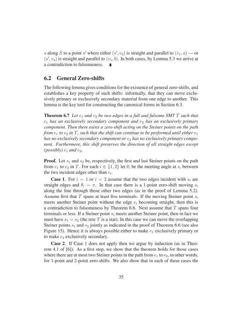
s along S to a point s′ where either (s′, v2) is straight and parallel to (v1, a) — or

(s′, v4) is straight and parallel to (v1, b). In both cases, by Lemma 5.3 we arrive at

a contradiction to fulsomeness.

6.2 General Zero-shifts

The following lemma gives conditions for the existence of general zero-shifts, and

establishes a key property of such shifts: informally, that they can move exclu-

sively primary or exclusively secondary material from one edge to another. This

lemma is the key tool for constructing the canonical forms in Section 6.3.

Theorem 6.7 Let e1 and e2 be two edges in a full and fulsome SMT T such that

e1 has an exclusively secondary component and e2 has an exclusively primary

component. Then there exists a zero-shift acting on the Steiner points on the path

from e1 to e2 in T , such that the shift can continue to be performed until either e1

has no exclusively secondary component or e2 has no exclusively primary compo-

nent. Furthermore, this shift preserves the direction of all straight edges except

(possibly) e1 and e2.

Proof. Let s1 and s2 be, respectively, the first and last Steiner points on the path

from e1 to e2 in T . For each i ∈ {1, 2} let θi be the meeting angle at si between

the two incident edges other than ei.

Case 1. For i = 1 or i = 2 assume that the two edges incident with si are

straight edges and θi = π. In that case there is a 1-point zero-shift moving si

along the line through those other two edges (as in the proof of Lemma 5.2).

Assume first that T spans at least five terminals. If the moving Steiner point si

meets another Steiner point without the edge ei becoming straight, then this is

a contradiction to fulsomeness by Theorem 6.6. Next assume that T spans four

terminals or less. If a Steiner point si meets another Steiner point, then in fact we

must have s1 = s2 (the tree T is a star). In this case we can move the overlapping

Steiner points s1 and s2 jointly as indicated in the proof of Theorem 6.6 (see also

Figure 15). Hence it is always possible either to make e1 exclusively primary or

to make e2 exclusively secondary.

Case 2. If Case 1 does not apply then we argue by induction (as in Theo-

rem 4.1 of [6]). As a first step, we show that the theorem holds for those cases

where there are at most two Steiner points in the path from e1 to e2, in other words,

for 1-point and 2-point zero-shifts. We also show that in each of these cases the

35

zero-shift strictly decreases the ratio of secondary material to primary material in

e1 and and strictly increases it in e2.

Case 2.1: 1-point zero-shifts. This case occurs where e1 and e2 are both inci-

dent with the same Steiner point s, that is, s2 = s1 = s. This is the same as the

situation illustrated in Figure 14. Let v be the neighbouring vertex to s1 that is

not an endpoint of e1 or e2. The zero-shift either moves s away from or towards

v. If s moves away from v then the lemma clearly holds. If s moves towards vthen the only problem that can occur is that the moving Steiner point may meet vbefore either e1 or e2 is straight. But in that case T is either not fulsome (if v is a

terminal) or we have two adjacent bent edges incident with a degree four Steiner

point, which is a contradiction to T being a SMT, by Lemma 5.1.

Case 2.2: 2-point zero-shifts. This case occurs where e1 and e2 are incident

with neighbouring Steiner points, s1 and s2. Firstly, suppose that e1 and e2 both

have the same colour. Then the 2-point zero-shift is a fundamental zero-shift, of

the sort illustrated in Figure 13b (where (s1, v2) = e1 and (s2, v4) = e2). This

zero-shift acts to decrease the the length of one of the edges e0 incident with s1

and s2 but not on the path from e1 to e2 (where (s1, v1) = e0 in the figure). It

immediately follows that the lemma holds, unless the length of e0 decreases to 0before either e1 or e2 is straight. However, in such a case the tree contains a degree

four Steiner point with an incident bent edge, and a second Steiner point, giving a

contradiction to minimality by Theorem 6.6.

Suppose, on the other hand, that e1 and e2 have different colours. Let e0

be the edge incident with s1 with the same colour as e2. If e0 is exclusively

primary, then an appropriate zero-shift can be constructed as follows. We can

apply a small 1-point zero-shift at s1, effectively transferring an arbitrarily small

exclusively secondary component to e0. More specifically, it strictly reduces the

secondary/primary material ratio in e1, and increases it in e0. Now there exists

a fundamental 2-point zero-shift between the secondary component of e0 and the

edge e2. Because the secondary component of e can be assumed to be arbitrarily

small, it follows that this second shift can reduce the secondary component of e0

to 0. Hence, together these two shifts give a zero-shift on the path between e1 and

e2, that preserves the direction of e0. The only remaining subcase is where e0 has

an exclusively secondary component, in which case we apply a similar argument,

but reverse the order of the two fundamental zero-shifts.

We now conclude the argument by induction on the number of Steiner points

in the path between e1 and e2, using the method of proof of Theorem 4.1 of [6],

which essentially generalises the construction in the previous paragraph. An im-

36

portant thing to note, in the inductive step, is that we can always find an edge

e0 with exclusively primary or exclusively secondary material and incident with

some s0 on the path between s1 and s2 such that the condition of Case 1 (θ0 = π)

does not apply at s0. This means that the required increase and decrease in sec-

ondary/primary material ratio occurs in the smaller zero-shift by the inductive

assumptions. The induction argument now follows easily.

Note that an immediate corollary of the proof of Theorem 6.7 is that any zero-

shift, other than the fundamental zero-shifts described in Section 6.1, can be de-

composed into two zero-shifts at least one of which acts on a strictly smaller set

of Steiner points. Hence, the only fundamental zero-shifts are those described in

Section 6.1.

6.3 Canonical Forms

The existence of zero-shifts makes it possible to transform any full and fulsome

SMT into another SMT with the same topology that has some well-defined canon-

ical form. In this section we outline the canonical forms proposed in [5] for the

uniform orientation metric and show that they also apply to Steiner trees for the

fixed orientation metric.

Definition 6.1 Given an ordering of the edges in a full Steiner topology T , an

SMT T for topology T is said to be canonical with respect to that ordering if Tcontains at most one bent edge and all primary edges and half-edges of T come

before secondary edges and half-edges of T under the ordering.

In a canonical tree there therefore exists a so-called transition edge (which is

possibly a bent edge), such that all edges that appear before the transition edge

wrt. the given ordering are primary and all edges appear after the transition edge

are secondary. Hence a canonical tree has at most one bent edge.

The proof of the following theorem follows immediately from the fact that we

can use zero-shifts to move primary/secondary components between edges in T .

(A detailed proof is given in [5], and it works without modifications for the more

general fixed orientation case.)

Theorem 6.8 Let a set terminals N and a full Steiner topology T for that set

of terminals be given. Suppose there exists a full and fulsome SMT for N with

topology T . Then for any ordering of the edges of T there exists a SMT for N(with topology T ) which is canonical with respect to that ordering.

37

primary

T2

r

T1

primary

secondary

primary

transition edge

secondary

Figure 16: Illustration of a tree T with the depth-first order canonical form. Pri-

mary edges are drawn as bold edges, and the remaining edges are secondary edges.

Depending on the chosen ordering, various canonical forms can be obtained [5].

From an algorithmic point of view, the depth-first ordering is the most important

one: Root T at some terminal r and order the edges as they appear in a depth-first

traversal of the tree from r. This results in a canonical form that is illustrated

in Figure 16. If we divide such a canonical tree T into two subtrees T1 and T2

by deleting the transition edge, the tree T2 that does not contain the root is sec-

ondary (i.e., all edges in T2 are secondary edges). Furthermore, the path p from

r to the transition edge is primary, while the subtrees that are attached to p either

are primary or secondary subtrees. These properties are used by the linear-time

algorithm for constructing a SMT for a given topology in Section 7.

By choosing another ordering of the edges, we obtain the following interesting

theorem [5]:

Theorem 6.9 Let T be a full and fulsome SMT for terminal set N with topology

T . Then there exists a SMT T ′ for terminal set N with topology T that uses at

most four legal orientations.

38

Proof. Order the edges of T by their colour; for example, the red edges may

come first in the ordering followed by the green edges and then the blue edges.

Consider a canonical SMT T ′ that comes from this ordering (by Theorem 6.8 such

a tree exists). Then it follows from the canonical form that the edges of any given

colour, not the same as the colour of the transition edge, are either all primary or

all secondary. Hence T ′ uses at most four legal orientations.

Finally, we note that the well-known Hwang canonical form for rectilinear

trees [12, 23] is a special case of the depth-first ordering canonical form. The

first observation is that by Lemma 6.5, in a fulsome and canonical rectilinear

SMT the topology of a full component must be a chain in which every Steiner

point is connected directly to at least one terminal. The Hwang topology form is

now obtained by rooting the topology in one end of the chain, and constructing

the depth-first ordering canonical form. The fact that there can be at most two

terminals in the subtree below the bent edge follows from the fullness of the tree.

7 Linear Time Algorithm for a Given Topology

By exploiting the concept of canonical forms, in this section we present a O(σn)time algorithm to compute a full and fulsome SMT T for a given full Steiner

topology T with n terminals (or show that no such tree exists). Our algorithm

is a generalisation of the algorithm by Brazil et al. [5] which works for uniform

orientation metrics with λ > 3 given orientations. In the following we denote

this the DFS-canonical algorithm, since it is based on the canonical form that

comes from a depth-first traversal of the topology T . Here we first present the

main algorithmic idea in Section 7.1. Then we show that the so-called merging

operation can be performed in constant time (Section 7.2), and in Section 7.3 we

briefly present the DFS-canonical algorithm and argue that it also works for the

general fixed orientation metric.

7.1 Labelling and Merging Algorithm

Consider the topology T shown in Figure 17. This topology has five terminals

t1, . . . , t5. We know from Section 5 that there exists a direction set U that is used

by every Steiner point in a full SMT T with topology T (assuming that such a

tree T exists). Assume furthermore that the primary/secondary labelling of the

edges in T is as in Figure 17. Hence the edge connecting, e.g., Steiner point s1

to terminal t1 is a straight edge with a primary direction from U ; however, the

39

primary

unknown

primary

secondary

secondary

primary

s2

t1

t2

t5

s3

t4

t3

primarys1

Figure 17: Labelling and bottom-up construction of SMT for a given topology

spanning five terminals.

colour of edge (s1, t1) is not known. Steiner point s1 is connected by straight

and labelled edges to two nodes (here terminals) with known positions. As will

be shown in Section 7.2, then in constant time we can either compute the unique

location of s1 — or decide that s1 cannot exist with the given direction set and

primary/secondary labelling.

The operation of computing the location of a node in T given the locations of

two of its neighbours is called a merging operation. If a direction set is given and

all edges except one have been labelled primary or secondary (as in Figure 17),

then we can compute a tree under this labelling or decide that no such tree exists

in O(n) time, where n is the number of terminals in T . We simply root T at the

unlabelled (transition) edge and merge nodes bottom-up in T . In Figure 17 we

could, e.g., first compute s1 based on t1 and t2, then s2 based on t3 and t4, then s3

based on s2 and t5, and finally construct the possibly bent transition edge based

40

on the positions of the Steiner points s1 and s3.

This is the main algorithmic idea employed in the linear-time algorithm. By

using the canonical forms that come from ordering the edges in T , the number of

possible labellings can be reduced from an exponential number — essentially two

possible labels per edge in the tree — to a linear number of possible labellings

(Section 7.3).

7.2 Constant-time Merging Operation

In this section we present the constant-time merging operation that facilitates the

efficient bottom-up construction outlined in Section 7.1. The lemma below was

originally proved only for uniform orientation metrics with λ > 3 [5]; here the

lemma is generalised to arbitrary fixed orientation metrics.

Lemma 7.1 Let T be a full SMT with full Steiner topology T , and let s be a

Steiner point in T . Assume that the locations in T of two of the neighbours of

s, u and v, are known; furthermore, assume that each edge (s, u) and (s, v) is

straight and has been labelled primary or secondary. Finally, assume that we

know the direction set for T . If Steiner point s exists in T and is not collinear with

u and v, then its location is unique and can be computed in constant time; also,

the colours of the edges (s, u) and (s, v) — and hence also the colour of the third

edge incident with s — are unique.

Proof. For the given direction set, we first make the following simple observa-

tions:

1. An exclusively primary edge and an exclusively secondary edge of the same

colour use adjacent orientations;

2. Every meeting angle is at most π.

Now suppose, contrary to the statement of the lemma, that it is possible to

construct two distinct Steiner points s and s′ adjacent to both u and v. Direct each

incident edge so that it is pointing outwards from s or s′. These incident edges use

four (not necessarily distinct) directions, all of which belong to a single direction

set. We will consider two cases, each of which show that we reach a contradiction

to one of the observations above.

Case 1. Suppose that s and s′ are not collinear with u or with v.

41

(a)

s's

vu

(b)

s'

s

vu

ab

c

d

Figure 18: Cases 1 and 2 in the proof of Lemma 7.1.

We will first show that the interiors of two of the edges intersect at a single

point. Consider the colours of the four edges (s, u), (s, v), (s′, u) and (s′, v). Since

there are only three colours, at least one colour (say, red) appears twice. Without

loss of generality, we can assume that (s, u) is a red edge. Then (s′, v) must also be

a red edge (since the other edge incident with u has the same primary/secondary

labelling as (s, u) but is not collinear, and the two edges incident with s have

distinct colours).

We introduce the following vectors (see Figure 18a):

a = −→su, b =−→s′v, c = −→sv, d =

−→s′u.

Assume the two red edges (s, u) and (s′, v) do not intersect. We will show that

the other two edges (s, v) and (s′, u) do intersect. Note that this occurs if and only

if there exist real numbers 0 < k1 < 1 and 0 < k2 < 1 satisfying the following

condition:

a = k1c + k2d. (4)

Also note that a− d = c − b, that is:

a + b = c + d. (5)

First suppose (s, u) and (s′, v) both use the same red direction, that is, b = kafor some k > 0. From equation (5) we obtain: a = (c+d)/(1+k) which satisfies

condition (4) where k1 = k2 = 1/(k + 1).On the other hand, suppose that (s, u) and (s′, v) use different red directions

(one exclusively primary and the other exclusively secondary). By Observation 1,

these are adjacent orientations, hence a and b are linearly independent. This

42

means there exist α1, α2, β1, β2 ∈ R such that c = α1a+α2b and d = β1a+β2b.

Since c and d do not use red directions, at least one of the αi’s and at least one

of the βi’s must be negative. By the symmetry of the equations we can assume,

without loss of generality, that α2 < 0. Substituting the expressions for c and d

into equation (5), we obtain:

a + b = (α1 + β1)a + (α2 + β2)b,

hence α1 + β1 = 1 and α2 + β2 = 1. Since α2 and at least one of the βi’s are

negative, it follows that there exist real numbers p, q > 0 such that:

α1 = 1 + p, α2 = −q, β1 = −p, β2 = 1 + q. (6)

Now, suppose we write a = k1c + k2d. To satisfy condition (4) we need to

show that this always has a real solution with 0 < k1 < 1 and 0 < k2 < 1.

Substituting in the expressions for c and d we obtain:

a = (k1α1 + k2β1)a + (k1α2 + k2β2)b.

Using the identities (6) and equating coefficients, we then get the following pair

of simultaneous equations:

k1(1 + p) + k2(−p) = 1

k1(−q) + k2(1 + q) = 0

Solving for k1 and k2 gives

k1 =1 + q

1 + p + q, k2 =

q

1 + p + q,

and hence we have 0 < k1 < 1 and 0 < k2 < 1.

We have now established that the interiors of two of the edges intersect at a

single point. We can assume that this pair of intersecting edges is (s, v) and (s′, u)(noting that we are no longer carrying across any of the previous assumptions

about colours of edges). This is the situation shown in Figure 18a.

If (s, v) and (s′, u) are the same colour, then the orientation corresponding

to the direction of (s, u) lies strictly between the directions of (s, v) and (s′, u)contradicting Observation 1. On the other hand, if (s, v) and (s′, u) have different

colours, then the remaining two edges must both use the third colour (since the

primary and secondary labelling of each edge is known). Hence, the four edges

43

(s, u), (s, v), (s′, u) and (s′, v) use three distinct colours. However, the four ver-

tices of the polygonal unit circle ∂D (centred at the origin) corresponding to the

directions of these four edges all lie in one of the open half planes on one side of

the line through the origin with direction−→ss′. This means that one of the meeting

angles is greater than π, contradicting Observation 2.

Case 2. The remaining possibility is that s and s′ are both collinear with

exactly one of the points u and v, say u (as in Figure 18b).

Since (s, v) and (s′, v) are either both primary or both secondary, it follows

that the two edges have different colours, while the edge (s′, u) must have the

third colour. As in Case 2, these three directions all lie in an open half plane,

again contradicting Observation 2.

We conclude that at most one Steiner point can be constructed.

Note that this construction can be done in constant time since the direction set

is known.

If s, u and v are collinear, then again the the colours of the edges (s, u), (s, v)and the third edge incident with s are uniquely determined, but the position of

s is not unique. This does not cause a problem in the bottom-up construction

algorithm due to Lemma 6.5. As a consequence of this lemma, at most one merg-

ing operation in the bottom-up construction algorithm can result in a non-unique

Steiner point s. In fact, this must then be the final merging operation where the

third edge incident to s (in addition to (s, u) and (s, v)) is the transition edge,

and the other end of this edge is a terminal t. This holds since the construction is

moving in towards the transition edge. What we can do here is leave the position

of the Steiner point undetermined and construct the transition edge by finding the

shortest edge connecting t to the line segment uv. Clearly, this can also be done

in constant time like an ordinary merging operation.

7.3 Linear-time DFS-canonical Algorithm

In this section we show how the linear-time construction algorithm from [5] can

be generalised to the fixed orientation metric. The algorithm uses the algorithmic

idea outlined in Section 7.1, and the constant-time merging operation from Sec-

tion 7.2. The algorithm is based on the depth-first traversal canonical form, and

therefore denoted the DFS-canonical algorithm.

The DFS-canonical algorithm runs in O(n) time for a given direction set U .

In Section 4 we showed that the number of possible direction sets is Θ(σ), and

44

that the direction sets furthermore can be determined in Θ(σ) time. By iterating

the O(n) time algorithm over all direction sets, we obtain a total running time of

O(σ + σn) which is O(σn).The idea of the DFS-canonical algorithm (for a given topology T and fixed

direction set U) is that if there exists a full and fulsome SMT T with full Steiner

topology T and direction set U , then T can be assumed to have the canonical form

that is illustrated in Figure 16. The algorithm consists of two depth-first traversals

of T from an arbitrary root terminal r:

1. Secondary subtrees are constructed bottom-up in T , that is, subtrees where

all edges are labelled as secondary edges. The merging operation is per-

formed bottom-up for each Steiner node; if a Steiner point cannot be con-

structed, then none of the ancestors of the node (relative to r) can con-

structed either.

2. Primary subtrees are constructed bottom-up in T . At the same time, each

edge in T is tried as potential transition edge. The idea is that it is possible

iteratively to construct the endpoints of the transition in constant time per

edge: The endpoint that is closest to the root r is constructed in the second

traversal, while the other endpoint is constructed in the first traversal of T(see Figure 16).

Full implementation details are given by Brazil et al. [5]. Thus we have the fol-

lowing theorem:

Theorem 7.2 Given a full Steiner topology T with n terminals and a fixed orien-

tation metric with σ legal orientations, then in O(σn) time we can either construct

a full and fulsome SMT T with topology T , or decide that no such tree exists.

8 Conclusion

The main contribution of this paper is to show the existence of powerful canonical

forms for SMTs for arbitrary (weighted) fixed orientation metrics. We also gave

efficient and simple algorithms to compute all direction sets for a given fixed ori-

entation metric, and to compute a SMT for a given full Steiner topology. Our re-

sults show that the two-phase exact algorithm for uniform orientation metrics [15]

easily can be adapted to general fixed orientation metrics. This would most likely

allow the efficient computation of large-scale SMTs for arbitrary fixed orientation

metrics.

45

Future research would focus on generalising our results further to metrics

given by piecewise differentiable unit circles — including proving the conjecture

that there in any normed plane and for any set of terminals exists a SMT where the

edges of each full component use at most three orientations (where the orientation

of an edge is defined by the straight line between the endpoints of the edge).

Acknowledgements

This work was partially supported by a grant from the Australia Research Council and by

a grant from the Danish Natural Science Research Council (51-00-0336).

References

[1] M. Brazil. Steiner Minimum Trees in Uniform Orientation Metrics. In D.-Z.

Du and X. Cheng, editor, Steiner Trees in Industries, pages 1–27. Kluwer

Academic Publishers, 2001.

[2] M. Brazil, D. A. Thomas, and J. F. Weng. Minimum Networks in Uniform

Orientation Metrics. SIAM Journal on Computing, 30:1579–1593, 2000.

[3] M. Brazil, D. A. Thomas, and J. F. Weng. Forbidden Subpaths for Steiner

Minimum Networks in Uniform Orientation Metrics. Networks, 39:186–

202, 2002.

[4] M. Brazil, D. A. Thomas, and J. F. Weng. Locally Minimal Uniformly Ori-

ented Shortest Networks. Discrete Applied Mathematics, 154:2545–2564,

2006.

[5] M. Brazil, D. A. Thomas, J. F. Weng, and M. Zachariasen. Canonical Forms

and Algorithms for Steiner Trees in Uniform Orientation Metrics. Algorith-

mica, 44:281–300, 2006.

[6] M. Brazil, P. Winter, and M. Zachariasen. Flexibility of Steiner Trees in

Uniform Orientation Metrics. Networks, 46:142–153, 2005.

[7] G. D. Chakerian and M. A. Ghandehari. The Fermat Problem in Minkowski

Spaces. Geometriae Dedicata, 17:227–238, 1985.

[8] H. Chen, C. K. Cheng, A. B. Kahng, I. I. Mandoiu, Q. Wang, and B. Yao.

The Y-Architecture for On-chip Interconnect: Analysis and Methodology. In

46

Proceedings ACM/IEEE International Conference on Computer-Aided De-

sign (ICCAD), pages 13–19, 2003.

[9] H. Chen, B. Yao, F. Zhou, and C. K. Cheng. The Y-Architecture: Yet An-

other On-chip Interconnect Solution. In Proceedings Asia and South Pacific

Design Automation Conference, pages 840–846, 2003.

[10] D.-Z. Du, B. Gao, R. L. Graham, Z.-C. Liu, and P.-J. Wan. Minimum Steiner

Trees in Normed Planes. Discrete and Computational Geometry, 9:351–370,

1993.

[11] M. Hanan. On Steiner’s Problem with Rectilinear Distance. SIAM Journal

on Applied Mathematics, 14(2):255–265, 1966.

[12] F. K. Hwang. On Steiner Minimal Trees with Rectilinear Distance. SIAM

Journal on Applied Mathematics, 30:104–114, 1976.

[13] F. K. Hwang, D. S. Richards, and P. Winter. The Steiner Tree Problem. An-

nals of Discrete Mathematics 53. Elsevier Science Publishers, Netherlands,

1992.

[14] H. Martini, K. J. Swanepoel, and G. Weiss. The Fermat-Torricelli Problem

in Normed Planes and Spaces. Journal of Optimization Theory and Appli-

cations, 115:283–314, 2002.

[15] B. K. Nielsen, P. Winter, and M. Zachariasen. An Exact Algorithm for the

Uniformly-Oriented Steiner Tree Problem. In Proceedings of the 10th Euro-

pean Symposium on Algorithms, Lecture Notes in Computer Science, volume

2461, pages 760–772. Springer, 2002.

[16] M. Sarrafzadeh and C. K. Wong. Hierarchical Steiner Tree Construction

in Uniform Orientations. IEEE Transactions on Computer-Aided Design,

11:1095–1103, 1992.

[17] K. J. Swanepoel. The Local Steiner Problem in Normed Planes. Networks,

36(2):104–113, 2000.

[18] S. Teig. The X Architecture: Not Your Father’s Diagonal Wiring. Inter-

national Workshop on System-Level Interconnect Prediction (SLIP), pages

33–37, 2002.

47

[19] P. Widmayer, Y. F. Wu, and C. K. Wong. On Some Distance Problems in

Fixed Orientations. SIAM Journal on Computing, 16(4):728–746, 1987.

[20] X Initiative Home Page. http://www.xinitiative.com, 2001.

[21] G. Xue and K. Thulasiraman. Computing the Shortest Network under a

Fixed Topology. IEEE Transactions on Computers, 51:1117–1120, 2002.

[22] M. C. Yildiz and P. H. Madden. Preferred Direction Steiner Trees. In Pro-

ceedings of the 11th Great Lakes Symposium on VLSI (GLSVLSI), pages

56–61, 2001.

[23] M. Zachariasen. Rectilinear Full Steiner Tree Generation. Networks,

33:125–143, 1999.

[24] M. Zachariasen. The Rectilinear Steiner Tree Problem: A Tutorial. In D.-

Z. Du and X. Cheng, editors, Steiner Trees in Industries, pages 467–507.

Kluwer Academic Publishers, Boston, 2001.

[25] M. Zachariasen. Comment on “Computing the Shortest Network under a

Fixed Topology”. IEEE Transactions on Computers, 55:783–784, 2006.

48