Astronomy&Astrophysics

A&A 635, A178 (2020)https://doi.org/10.1051/0004-6361/201937107© ESO 2020

The solar wind from a stellar perspective

How do low-resolution data impact the determination of wind properties?

S. Boro Saikia1, M. Jin2,3, C. P. Johnstone1, T. Lüftinger1, M. Güdel1, V. S. Airapetian4,5,K. G. Kislyakova1, and C. P. Folsom6

1 University of Vienna, Department of Astrophysics, Türkenschanzstrasse 17, 1180 Vienna, Austriae-mail: sudeshna.boro.saikia@univie.ac.at

2 Lockheed Martin Solar and Astrophysics Laboratory, Palo Alto, CA 94304, USA3 SETI institute, Mountain View, CA 94043, USA4 Sellers Exoplanetary Environments Collaboration, NASA Goddard Space Flight Center, Greenbelt, USA5 American University, Washington DC, USA6 IRAP, Université de Toulouse, CNRS, UPS, CNES, 14 Avenue Edouard Belin, 31400 Toulouse, France

Received 13 November 2019 / Accepted 5 February 2020

ABSTRACT

Context. Due to the effects that they can have on the atmospheres of exoplanets, stellar winds have recently received significantattention in the literature. Alfvén-wave-driven 3D magnetohydrodynamic models, which are increasingly used to predict stellar windproperties, contain unconstrained parameters and rely on low-resolution stellar magnetograms.Aims. In this paper, we explore the effects of the input Alfvén wave energy flux and the surface magnetogram on the wind propertiespredicted by the Alfvén Wave Solar Model (AWSoM) model for both the solar and stellar winds.Methods. We lowered the resolution of two solar magnetograms during solar cycle maximum and minimum using spherical harmonicdecomposition. The Alfvén wave energy was altered based on non-thermal velocities determined from a far ultraviolet spectrum of thesolar twin 18 Sco. Additionally, low-resolution magnetograms of three solar analogues, 18 Sco, HD 76151, and HN Peg, were obtainedusing Zeeman Doppler imaging and used as a proxy for the solar magnetogram. Finally, the simulated wind properties were comparedto Advanced Composition Explorer (ACE) observations.Results. AWSoM simulations using well constrained input parameters taken from solar observations can reproduce the observed solarwind mass loss and angular momentum loss rates. The simulated wind velocity, proton density, and ram pressure differ from ACEobservations by a factor of approximately two. The resolution of the magnetogram has a small impact on the wind properties andonly during cycle maximum. However, variation in Alfvén wave energy influences the wind properties irrespective of the solar cycleactivity level. Furthermore, solar wind simulations carried out using the low-resolution magnetogram of the three stars instead of thesolar magnetogram could lead to an order of a magnitude difference in the simulated solar wind properties.Conclusions. The choice in Alfvén energy has a stronger influence on the wind output compared to the magnetogram resolution.The influence could be even stronger for stars whose input boundary conditions are not as well constrained as those of the Sun.Unsurprisingly, replacing the solar magnetogram with a stellar magnetogram could lead to completely inaccurate solar wind properties,and should be avoided in solar and stellar wind simulations. Further observational and theoretical work is needed to fully understandthe complexity of solar and stellar winds.

Key words. solar wind – stars: winds, outflows – turbulence – magnetohydrodynamics(MHD)

1. Introduction

Stellar magnetic fields are responsible for a large number of phe-nomena, including the emission of high-energy radiation andthe formation of supersonic ionised winds. By driving atmo-spheric processes such as non-thermal losses to space, thesewinds play an important role in the evolution of planetary atmo-spheres and habitability (Tian et al. 2008; Kislyakova et al.2014a; Airapetian et al. 2017). As an example, the strong solarwind of the young Sun (Johnstone et al. 2015a; Airapetian &Usmanov 2016) in combination with the weaker magnetic fieldof early Earth (Tarduno et al. 2010) led to higher compressionof the Earth’s magnetosphere. This resulted in wider open-ing of polar ovals and higher atmospheric escape rates than atpresent (Airapetian et al. 2016). It has been shown that plane-tary atmospheric loss in planets with a magnetosphere depends

on the interplay between the solar wind strength, wind cap-ture area of the planetary magnetosphere, and the ability of themagnetosphere to recapture the atmospheric outflow, althoughthe effect of magnetospheric compression on atmospheric lossrates are currently up for debate (Blackman & Tarduno 2018).For planets lacking any intrinsic magnetic field, the incomingstellar wind interacts directly with the atmosphere, leading toatmospheric escape through the plasma wake and from a bound-ary layer of the induced magnetosphere (Barabash et al. 2007;Lundin 2011). Venus-like CO2-rich atmospheres are less proneto expansion and escape, but they are still sensitive to enhancedX-ray and extreme ultraviolet (XUV) fluxes, and wind erosion(Lichtenegger et al. 2010; Johnstone et al. 2018). The same canbe true for exoplanets orbiting young stars with stronger stel-lar winds leading to efficient escape of the atmosphere to space(Wood et al. 2002; Lundin 2011). It is therefore important to

Article published by EDP Sciences A178, page 1 of 21

A&A 635, A178 (2020)

investigate stellar wind properties in Sun-like stars to under-stand their impact on habitability and also provide constraintson planetary atmospheres.

Observations of the solar wind taken by satellites such asthe Advanced Composition Explorer (ACE, Stone et al. 1998;McComas et al. 1998) and Ulysses (McComas et al. 2003) havegreatly improved our knowledge and understanding of the solarwind properties. The solar wind can be broken down into thefast and the slow wind with median wind speeds of approxi-mately 760 and 400 km s−1 respectively (McComas et al. 2003;Johnstone et al. 2015b). The fast component arises from coro-nal holes and the slow component is launched from areas aboveclosed field lines, and from the boundary regions of open andclosed field lines (Krieger et al. 1973). As the magnetic geometryof the Sun changes during the solar cycle, the locations of the fastand slow components change without any considerable changesin their properties, such as speed or mass flux. In situ measure-ments by spacecrafts such as Ulysses and Voyager have foundthat the mass loss rate of the solar wind is ∼2× 10−14 M� yr−1,and that it changes by a factor of only two over the solar cycle(Cohen 2011). Angular momentum loss rates vary by 30–40%over the solar cycle as shown by Finley et al. (2018). This showsthat despite the dramatic change in the surface magnetic field ofthe Sun during the cycle, the changes in the solar wind propertiesare not drastic.

Unfortunately, direct measurements of the properties of low-mass stellar winds are not available; instead techniques toindirectly measure stellar winds must be used, including recon-structing astrospheric Ly-α absorption (Wood et al. 2001) andfitting rotational evolution models to observational constraints(Matt et al. 2015; Johnstone et al. 2015a). This is problematic forstellar wind modelling since we can neither constrain the modelfree parameters nor test our results observationally. Attemptshave been made to detect radio free-free emissions due to thepresence of stellar winds in Sun-like stars (Drake et al. 1993;van den Oord & Doyle 1997; Gaidos et al. 2000; Villadsen et al.2014; Fichtinger et al. 2017). Unfortunately there has been nodetection so far but radio observations have provided impor-tant upper limits on the wind mass loss rates of a handful ofSun-like stars. X-ray emission due to charge exchange betweenionised stellar winds and the neutral interstellar hydrogen havealso been used to provide upper limits on the mass loss rate dueto stellar winds (Wargelin & Drake 2002). For a limited sampleof close-in transiting hot Jupiters, Lyman-α observations havebeen used to estimate the properties of the wind of the host star(Kislyakova et al. 2014b; Vidotto & Bourrier 2017). The indi-rect method of astrospheric Lyman-αmeasurements (Wood et al.2001, 2005; Wood 2004) is the only technique that has providedobserved wind mass loss rates for some nearby Sun-like stars.Using this method Wood et al. (2005) showed that the mass lossrate has a power-law relation with magnetic activity, implyingthat more active stars have higher mass loss rates. Some starsdo not appear to follow this trend and this method can only beapplied to nearby stars that are surrounded by at least partiallyneutral interstellar medium. We are therefore heavily dependenton wind models to enhance our understanding of stellar windproperties.

Solar and stellar wind modelling faces multiple challenges,as we still lack a complete understanding of the heating, acceler-ation, and propagation of the wind. The outward acceleration ofthe wind takes place in large part due to thermal pressure gradi-ents driven by the very large temperatures of coronal gas (Parker1958). However, measurements of the gas temperatures insidecoronal holes show that the temperatures are not high enough

to accelerate the wind to the speed of the fast component, andtherefore another acceleration mechanism is required (Cranmer2009). The source of the wind heating and the nature of thisadditional acceleration mechanism are currently poorly under-stood (Cranmer & Winebarger 2019). Alfvén waves are consid-ered to be a likely key mechanism for solar wind heating andacceleration. Observations taken using Hinode (Kosugi et al.2007) and the Solar Dynamics Observatory (SDO, Pesnell et al.2012) have shown that Alfvénic waves in the solar chromo-sphere have much stronger amplitudes compared to their coronalcounterpart (De Pontieu et al. 2007; McIntosh et al. 2011). Theweakening of the waves as they reach the corona is attributed tothe wave dissipation. The waves reflected by density and mag-netic pressure gradients interact with the forward propagatingwaves resulting in wave dissipation, which in turn heats thelower corona. This provides the necessary energy to propagateand accelerate the wind so that it can escape from the gravityof the star (Matthaeus et al. 1999). It has been suggested thatfor very rapidly rotating stars, magneto-centrifugal forces alsoprovide an important wind acceleration mechanism (Johnstone2017).

To tackle the wind heating problem, it has been common insolar and stellar wind models to assume a polytropic equationof state (Parker 1965; van der Holst et al. 2007; Cohen et al.2007; Johnstone et al. 2015b), which states that the pressure,p, is related to the density, ρ, by p ∝ ρα, where α is the poly-tropic index and is typically taken to be α ∼ 1.1. This leads tothe wind being heated implicitly as it expands. Free parametersin these models are the density and temperature at the base of thewind and the value of α, all of which can be constrained for thesolar wind from in situ measurements (Johnstone et al. 2015b).However, these parameters are unconstrained for the winds ofother stars. An alternative is to use solar and stellar wind modelsthat incorporate Alfvén waves, which are becoming increasinglypopular (Cranmer & Saar 2011; Suzuki et al. 2013). Some ofthe earliest Alfvén-wave-driven models date back to Belcher &Davis (1971), and Alazraki & Couturier (1971). Multiple groupshave developed 1D (Suzuki & Inutsuka 2006; Cranmer et al.2007), 2D (Usmanov et al. 2000; Matsumoto & Suzuki 2012),and 3D (Sokolov et al. 2013; van der Holst et al. 2014; Usmanovet al. 2018) Alfvén-wave-driven solar wind models that can suc-cessfully simulate the current solar wind mass loss rates. In thiswork the 3D magnetohydrodynamic (MHD) model Alfvén WaveSolar Model (AWSoM; van der Holst et al. 2014) is used, whereAlfvén wave propagation and partial reflection leads to a tur-bulent cascade, heating and accelerating the wind. The Alfvénwave energy is introduced using an input Alfvén wave Poyntingflux ratio (S A/B, where B is the magnetic field strength at theinner boundary of the simulation). For the Sun, Sokolov et al.(2013) established S A/B to be 1.1 × 106 Wm−2 T−1. In stellarwind models, S A/B is modified using scaling laws between theX-ray activity and magnetic field B of the star (Pevtsov et al.2003; Garraffo et al. 2016; Dong et al. 2018), which requiresprior information about the former parameter. As stellar X-rayactivity is known to exhibit variations, this approach will alsolead to variation in S A/B for a magnetically variable star. In thesolar case, the Poynting flux is well constrained from observa-tions and nearly constant for all solar simulations. The value ofS A/B is an important input parameter, but how a change in thePoynting flux ratio quantitatively changes the final wind outputremains unknown. It is important to understand the relationshipbetween S A/B and the coronal and wind properties, as often thePoynting flux ratio is a difficult parameter to directly determinefrom stellar observations.

A178, page 2 of 21

S. Boro Saikia et al.: Solar wind

In 3D MHD solar wind models such as AWSoM, the inputstellar surface magnetic field ensures that the model includesthe correct magnetic topology of the stellar wind. In the caseof the Sun, multiple solar observatories produce high-resolutionsynoptic magnetograms which can be used as an input (Rileyet al. 2014). Stellar wind models use low-resolution magneticmaps of stars as input (Vidotto et al. 2011, 2014; Nicholsonet al. 2016; Alvarado-Gómez et al. 2016a,b; Garraffo et al. 2013,2015, 2016; Fionnagáin et al. 2019), which are reconstructedusing the technique of Zeeman Doppler imaging (ZDI; Semel1989). This imagining technique reconstructs the large-scalefield using spectropolarimetric observations, where the field istypically described using spherical harmonic expansion. Alter-natively, solar magnetograms are sometimes used as a proxy fora given Sun-like star and are scaled to its magnetic field andactivity (Dong et al. 2018). One disadvantage of using ZDI stel-lar magnetic maps is their resolution. A typical stellar magneticmap is reconstructed up to a spherical harmonics degree, lmax,of 5–10, while a solar magnetogram can have lmax ≥100. It isnot known how the resolution of the magnetograms and the useof the Sun as a stellar proxy influence stellar wind propertiesdetermined from AWSoM simulations.

In this study we validate AWSoM under low-resolutioninput conditions, which is an important pre-requisite for theuse of AWSoM in stellar cases. We investigate whether or notAWSoM solar wind simulations under low-resolution input con-ditions can reproduce observed ACE1 solar wind properties at1 AU. Under high-resolution input conditions, AWSoM windproperties show strong agreement with observed wind prop-erties (Oran et al. 2013; Sachdeva et al. 2019). We carry outwind simulations using low-resolution input magnetograms anda varying S A/B ratio to investigate the sensitivity of these twoinput parameters in determining wind properties. Low-resolutionmagnetograms are obtained by performing spherical harmonicdecompositions of high-resolution solar Global Oscillation Net-work Group (GONG)2 magnetograms for lmax = 150, 20, 10, and5. We also obtain different values of S A/B from far ultravio-let (FUV) spectral lines. The different values of lmax and S A/Bare used to create two grids of AWSoM wind simulations duringminimum and maximum of the solar cycle. Additionally, we alsouse ZDI maps of three solar analogues as a replacement for thesolar magnetic field to investigate whether or not input magne-tograms of stars with similar properties can be used as a proxy.In Sect. 2, the wind model is introduced. In Sect. 3, we describeour grid of simulations. In Sects. 4 and 5, we discuss our resultsand conclusions.

2. Model description

We use the data-driven AWSoM model of the 3D MHD codeBlock Adaptive Tree Solar Roe-Type Upwind Scheme (BATS-R-US; Powell et al. 1999), which is publicly available under theSpace Weather Modelling Framework (SWMF; Tóth et al. 2012).Alfvén wave partial reflection and dissipation lead to the heatingof the plasma, thus no polytropic heating function is requiredin this model. Thermal and magnetic pressure gradients lead toacceleration of the wind. The model incorporates two energyequations for protons and electrons with the same proton andelectron velocities. In addition to radiative cooling, collisional

1 http://www.srl.caltech.edu/ACE/ASC/. Data accessed inOctober 2019.2 https://gong.nso.edu/data/magmap/crmap.html

heat conduction (Spitzer 1956) is included near the star (≤5 R�)and collisionless heat conduction (Hollweg 1978) is adopted faraway from the star (>5 R�).

The simulation framework consists of multiple modules.Here, we use the solar corona (SC) and the inner heliosphere(IH) module. The simulation setup for the SC module consists ofa 3D spherical grid with an inner boundary immediately abovethe stellar radius in the upper chromosphere (default at ≥1 R�)and the outer boundary is at a distance of 25 R�. To resolve thetransition region, the heat conduction and radiative cooling ratesare artificially modified as discussed in detail by Sokolov et al.(2013). The IH module starts at 18 R� and extends beyond 1 AU.There is a coupling overlap between the two modules. The sim-ulation uses spherical block-adaptive grid in SC from 1 R� to 24R� (grid blocks consist of 6× 4× 4 mesh cells) and Cartesiangrid in IH (grid blocks consist of 4× 4× 4 mesh cells). Thesmallest cell size is 0.001 R� near the star and 1 R� at the SCouter boundary. In IH, the smallest cell is 0.1 R� and largest cellis 8 R�. For both SC and IH, adaptive mesh refinement (AMR) isperformed to resolve the current sheets in the simulation domain(for a detailed description of the model, see Sokolov et al. 2013and van der Holst et al. 2014).

The solar or stellar surface magnetic field is one of the keylower boundary conditions. A potential field extrapolation is car-ried out using a potential field source surface (PFSS) modelto obtain the initial magnetic field condition in the simulationdomain. The source surface radius is kept at 2.5 R�. The Alfvénwave Poynting flux is injected at the base of the simulation toheat and accelerate the wind. The Alfvén wave Poynting fluxS A/B is usually set to be 1.1× 106 W m−2 T−1. Here, we investi-gate how a change in the value of S A/B and the resolution of thesolar surface magnetic field alter the simulated wind properties.

The model includes multiple other input parameters, such asthe base density and temperature, the stochastic heating term,and the transverse correlation length of the Alfvén wave. Thebase density and temperature are fixed at 3× 10−11kg m−3 and50 000 K respectively. Many stellar wind models use the temper-ature at the lower boundary as a free parameter and scale thisvalue to stars based on measurements of coronal temperatures,which have been observed to depend on the star’s activity level(Holzwarth & Jardine 2007; Johnstone & Güdel 2015). However,the base temperature in our model is not the coronal tempera-ture, and our results are not strongly sensitive to the choice ofthis value. The stochastic heating term hS was taken to be 0.17and determines the energy partitioning between the electrons andprotons in the model, which is from a linear wave theory byChandran et al. (2011) and is kept constant in this work. Thetransverse correlation length of the Alfvén waves L⊥ in the planeperpendicular to the magnetic field B is responsible for partialreflection of forward-propagating Alfvén waves required to formthe turbulent cascade. The value of L⊥

√B used in this model is

1.5× 105 m√

T and is an adjustable input parameter.We use two input magnetograms to simulate wind proper-

ties at solar cycle maximum and minimum, Carrington rotationCR 2159 and CR 2087, respectively. The magnetograms areinput into the simulations in the form of spherical harmonicdecomposition. The maximum spherical harmonics degree con-sidered determines the resolution of the magnetogram andtherefore the minimum size of the magnetic features on the stel-lar surface. For the highest resolution simulation in this study,the spherical harmonics degree lmax is truncated to 150 andS A/B = 1.1× 106 W m−2 T−1. The rest of the input parametersare listed in Table 1 and taken from van der Holst et al. (2014).

A178, page 3 of 21

A&A 635, A178 (2020)

Table 1. Input parameters.

Parameters Value

S A/B 1.1× 106 W m−2 T−1

ρ 3× 10−11kg m−3

T 50 000 KL⊥√

B 1.5× 105 m√

ThS 0.17

3. Two grids of low-resolution solar windsimulations

To investigate the dependence of solar wind properties on low-resolution data, we created two grid of simulations. Only theinput magnetogram resolution and the Alfvén wave Poyntingflux ratio (S A/B) were altered and the rest of the input boundaryconditions (Table 1) were kept constant. The two grids of sim-ulations, the first grid during solar cycle maximum (CR 2159)and the second during minimum (CR 2087), were created bycarrying out spherical harmonic decompositions of the inputmagnetogram for four different values of the maximum harmon-ics degree, lmax = 150, 20, 10, and 5. Additionally, four differentvalues of the S A/B ratio were used, where one S A/B was takenfrom Sokolov et al. (2013) and the remaining three S A/B val-ues were determined from three different FUV spectral lines ofthe solar twin 18 Sco. The grid setup is identical for both solarmaximum and minimum. Furthermore, we explored the use of aproxy magnetogram by including ZDI large-scale magnetic mapsof three solar analogues instead of an input solar magnetic fieldto AWSoM.

3.1. Spherical harmonics decomposition of CR 2159and CR 2087

Stellar magnetograms reconstructed using ZDI have a muchlower resolution compared to solar magnetograms. The majorityof the stellar magnetograms have lmax ≤ 10. We used sphericalharmonics decomposition on two different solar magnetogramsto bring their resolution down to ZDI level. The magnetogramswere obtained during solar cycle maximum and minimum,CR 2159 and CR 2087 respectively (Fig. 1, top). The synopticmagnetograms were obtained using GONG, where the pho-tospheric field is considered to be purely radial. We carriedout spherical harmonic decompositions on the synoptic magne-tograms using the PFSS model available in BATS-R-US (Tóthet al. 2011). The output is a set of complex spherical harmonicscoefficients αlm for a range of spherical harmonics degrees l =0,1, ...., lmax.

The αlm coefficients were used to calculate Br(θ, φ) for lmax =150, 20, 10, and 5 based on Eq. (1) (Vidotto 2016),

Br(θ, φ) =lmax∑l=1

l∑m=0

αlmYlm(θ, φ), (1)

Ylm = clmPlm(cos θ)eimφ, (2)

clm =

√2l + 1

4π(l + m)!(l − m)!

, (3)

where Plm(cos θ) is the Legrende polynomial associated withdegree l and order m and clm is a normalisation constant. The

summation is carried out over 1≤ l≤ lmax and −l ≤ m ≤ l. Theabove equations are also implemented in the ZDI technique(Donati et al. 2006), where large-scale stellar surface mag-netic geometry is reconstructed by solving for Br(θ, φ)3, oftenusing lower values of spherical harmonics order, lmax ≤ 10. Weused Eqs. (1)–(3) to obtain low-resolution magnetograms byrestricting lmax to 150, 20, 10, and 5.

Figure 1 shows the synoptic GONG magnetograms followedby the low-resolution reconstructions for both CR 2159 (leftcolumn) and CR 2087 (right column). The magnetograms recon-structed by restricting lmax to 5 and 10 are representative ofsolar large-scale magnetograms and can be considered similarto a ZDI magnetic map of the Sun (Kochukhov et al. 2017).The radial magnetic field geometry was extrapolated into a 3Dcoronal magnetic field by using a PFSS solution as a startingcondition for the simulations. Either spherical harmonics or afinite difference potential field solver (FDIPS) can be used. Tóthet al. (2011) showed that it is preferable to use FDIPS over spher-ical harmonics as ring patterns are sometimes seen near strongmagnetic field regions when the spherical harmonics techniqueis used, specifically for higher values of lmax. We used sphericalharmonics to be consistent with ZDI large-scale stellar magne-tograms. Additionally, we are interested in low values of lmax,where the impact is minimal.

3.2. Alfvén wave Poynting flux to B ratio (SA/B)

The Poynting flux to B ratio (S A/B) is a key input parameterthat characterises the heating and acceleration of the wind. For asolar wind simulation using AWSoM, the S A/B ratio was set bySokolov et al. (2013) to be 1.1× 106 W m−2 T−1. In stellar windmodelling using AWSoM, S A/B is sometimes adapted based onscaling laws between magnetic flux and X-ray flux (Garraffoet al. 2016; Dong et al. 2018). In this work, we investigated howthe S A/B ratio influences the mass and angular momentum lossrates, and other wind properties such as wind velocity, density,and ram pressure.

In the case of the Sun, the Alfvén wave Poynting flux S A canbe determined if we know the Alfvén speed VA and the waveenergy density w,

S A = VAw, (4)

VA = B/√µ0ρ, (5)

under the assumption of equipartition of kinetic and thermalenergies of Alfvén waves, the wave energy density w can beexpressed as,

w = ρδv2, (6)

resulting in the following S A/B ratio,

S A/B = ρδv2/√µ0ρ, (7)

where ρ is the base density, δv2 is the turbulent perturba-tion, and µ0 is the magnetic permeability of free space. Theturbulent perturbation is related to the non-thermal turbulentvelocity, ξ2 = 1

2 〈δv2〉 (Banerjee et al. 1998). If we know thenon-thermal velocity and base density for a given star, we canestimate the S A/B ratio. Both of these quantities can be esti-mated using FUV spectra of stars using spectral lines that areformed in the upper chromosphere or transition region. Works by

3 ZDI studies also reconstruct the azimuthal Bφ(θ, φ) and meridionalfield Bθ(θ, φ), which are not used in this work.

A178, page 4 of 21

S. Boro Saikia et al.: Solar wind

Fig. 1. Synoptic GONG magnetograms during solar cycle maximum, CR 2159 (top left) and cycle minimum, CR 2087 (top right) followed by thespherical harmonic reconstructions with lmax = 150, 20, 10, and 5 respectively (second row to bottom). The magnetic maps are saturated to differentvalues of Br, to highlight the surface magnetic features.

Banerjee et al. (1998), Pagano et al. (2004), Wood et al. (1997),and Oran et al. (2017) have shown that the non-thermal velocitiescan be determined from FUV spectral line broadening. Howeverthe S A/B determined from FUV spectra will strongly depend onthe spectral line used and can vary significantly even for the samestar. Non-thermal velocities in the Sun can vary in a range of10–30 km s−1 (De Pontieu et al. 2007), where the distributionpeaks at 15 km s−1.

Here, we kept the base density of the solar wind constant(Table 1) and only changed the value of the non-thermal velocityin Eq. (7). The non-thermal velocity was modified based on the

analysis of three different spectral lines: Si IV at 1402 Å, Si IV

1393 Å, and O IV 1401 Å. A Hubble Space Telescope (HST)spectrum of the solar twin 18 Sco (HD146233) was used asa solar proxy (Fig. 2), instead of the Interface Region Imag-ing Spectrograph (IRIS) solar observations to ensure that thenon-thermal velocities used in this work have similar uncertaintylevel as for other stars. IRIS is also not a full disk instru-ment although it produces full disk mosaic of the Sun once permonth4. The star 18 Sco was chosen as it is a well-known solar4 https://iris.lmsal.com/mosaic.html

A178, page 5 of 21

A&A 635, A178 (2020)

Fig. 2. HST FUV spectrum of 18 Sco. The spectral lines used in thisanalysis are marked.

Table 2. Formation temperature and non-thermal velocity for the threeFUV spectral lines and the corresponding S A/B ratios.

Spectral line Wavelength Ti ξ S A/B[Å] [K] [km s−1] [W m−2 T−1]

Si IV 1393.75 60 000 29.6 2.2 × 106

Si IV 1402.77 60 000 26.6 2.0 × 106

O IV 1401.16 50 000 16.0 1.2 × 106

twin with a similar rotation rate as the Sun (Porto de Mello &da Silva 1997).

We determined the non-thermal velocity by carrying out adouble Gaussian fit to our three selected spectral lines, wherethe full width at half maximum (FWHM) of the narrow com-ponent of the fit gives ξ. The non-thermal velocity is assumedto be purely due to transverse Alfvén waves and can be usedto determine the turbulent velocity perturbation δv2 (Oran et al.2017). Figure A.1 shows the Si IV line at 1393.75 Å and the dou-ble Gaussian fit to the line. Table 2 lists the ξ for each of the threespectral lines used. According to Wood et al. (1997), the nar-row component of the line profile accounts for the non-thermalvelocity while the broad component could be attributed to micro-flaring, though Ayres (2015) showed that the origin of the broadcomponent is not entirely clear and could be due to chromo-spheric bright points (Peter 2006). However, we note that in redgiants the enhanced broadening near the wings is attributed toboth radial and tangential turbulence produced by Alfvén waves(Carpenter & Robinson 1997; Robinson et al. 1998; Airapetianet al. 2010).

We used Eq. (8) to determine the non-thermal velocity fromthe measured FWHM (Banerjee et al. 1998; Oran et al. 2017),which is then used to determine S A/B. The FWHM is given by,

FWHM =

√4 ln 2

(λ

c

2) (2kBTi

Mi+ ξ2

), (8)

where FWHM is the full width half maximum of the narrowcomponent of the double Gaussian fit, λ is the rest wavelengthof the spectral line in Å, c is the speed of light in km s−1, kB is

the Boltzmann constant, Mi is the atomic mass of the element,and Ti is the formation temperature in K. We fitted both singleand double Gaussian line profiles and used a χ2 test to deter-mine the goodness of fit. The fit is always better when a doubleGaussian profile is used.

The non-thermal velocity determined using the O IV lineis in good agreement with the peak solar non-thermal velocityof 15 km s−1 (De Pontieu et al. 2007). The estimated ξ usingthe Si IV lines are much higher. According to Phillips et al.(2008) the non-thermal velocity might depend on the heightabove the solar limb. The formation temperature of the O IV lineis 50 000 K, which is also the base temperature of our simu-lation grid. This non-thermal velocity results in a S A/B that isvery close to the well calibrated S A/B of Sokolov et al. (2013).The formation temperatures of the Si lines are slightly higherand lead to a higher ξ as listed in Table 2. Investigation ofsolar non-thermal velocity at different heights by Banerjee et al.(1998) shows that the non-thermal velocity could be as high as46 km s−1 and changes with height. This could be linked to thedamping of Alfvén waves as they move from the chromosphereto the corona due to wave reflection and dissipation. A detaileddiscussion on these different line formations is however beyondthe scope of this work.

In the solar case, direct observations of the solar chromo-sphere and corona have lead to a detailed understanding ofnon-thermal velocities in the upper atmosphere. We can com-pare the non-thermal velocities obtained from FUV spectra withdirect spatial observations. However, stellar observations lackthe spatial and temporal resolution of the Sun. It becomes dif-ficult to determine which out of the many non-thermal velocitiesavailable should be used to estimate S A/B. Therefore, we ransimulations of the solar wind by scaling S A/B using the threedifferent non-thermal velocities given in Table 2 to investigateits influence on the wind properties.

3.3. Stellar magnetic maps as a proxy for the solarmagnetogram

Currently, ZDI (Semel 1989; Brown et al. 1991; Donati & Brown1997; Piskunov & Kochukhov 2002; Kochukhov & Piskunov2002; Folsom et al. 2018) is the only technique that can recon-struct the surface magnetic geometries of stars. It is a tomo-graphic technique that reconstructs the large-scale magneticgeometry of stars from circularly polarised spectropolarimetricobservations. It is an inverse method where a magnetic map isreconstructed by inverting observed spectropolarimetric spectra,where the surface magnetic field is described as a combinationof spherical harmonic components (Donati et al. 2006) using thesame equations as in Sect. 3.1 (see Folsom et al. 2018, for moredetails).

As ZDI only reconstructs the large-scale magnetic field, themagnetic maps are generally limited to lmax ≤ 10. As a result,the small-scale magnetic field cancel out and the global mag-netic field is much weaker than in typical solar magnetograms.These ZDI magnetic maps are used as input magnetograms forstellar wind studies, where the global magnetic field strength issometimes artificially increased to account for the loss of small-scale features. Since ZDI magnetic maps are only available for ahandful of stars, it is often necessary to use a ZDI map from astar with similar parameters as a proxy, and scale it. However, themagnetic geometry of any two stars is different. Furthermore, themagnetic geometry of active Sun-like stars can evolve over veryshort time-scales (Jeffers et al. 2017; Rosén et al. 2016). Eventhe solar large-scale magnetic geometry changes complexity over

A178, page 6 of 21

S. Boro Saikia et al.: Solar wind

Table 3. Stellar parameters of the sample.

Name Mass Radius Inclination Prot

[M�] [R�] [◦] [days]

18 Sco 0.98± 0.13 1.022± 0.018 70 22.7HD76151 1.24± 0.12 0.979± 0.017 30 20.5HN Peg 1.085± 0.091 1.002± 0.018 75 4.6

Notes. The masses and radii are taken from Valenti & Fischer (2005)and the rotation periods are taken from Petit et al. (2008) and BoroSaikia et al. (2015).

the solar cycle, although the complexity of the solar magneticfield does not lead to any significant changes in the solar windmass loss rate. It is not known if the same is true for very activeSun-like stars.

Due to the availability of observational constraints, our Sunis the best test case to investigate whether or not ZDI magneticmaps of solar analogues can be used as a solar proxy. If the sim-ulated solar wind properties cannot be reproduced using a ZDImap of a solar analogue as a solar proxy, then it is very unlikelythat the use of the Sun as a proxy for a cool star such as anM dwarf is reliable. The three solar proxies used in this workare 18 Sco, HD 76151, and HN Peg. With a rotation period of22.7 days, 18 Sco is the only solar twin for which a large-scaleZDI surface magnetic reconstruction is available (Petit et al.2008). HD76151 is a solar mass star and is rotating slightly fasterthan the Sun with a rotation period of 20.5 days (Petit et al.2008). HN Peg is a young solar analogue and is rotating muchfaster than the Sun at 4.6 days (Boro Saikia et al. 2015). Table 3lists the stellar parameters of the sample. The large-scale mag-netic geometries of 18 Sco and HD76151 were reconstructed byPetit et al. (2008). The spectropolarimetric data are available aspart of the open-source archive POLARBASE (Petit et al. 2014).We applied ZDI (Folsom et al. 2018) on the POLARBASE datato obtain the maps in Fig. 3. The magnetic map of HN Peg wastaken from Boro Saikia et al. (2015). Figure 3 shows the large-scale radial magnetic field of the sample, where each map wasreconstructed with lmax ≤ 10. We used the magnetic maps inFig. 3 instead of an input solar magnetogram and carried outsteady-state wind simulations. The other input parameters, suchas S A/B, density, and temperature, were taken from Table 1.

4. Results and discussion

4.1. Properties of the solar wind during solar cycle minimumand maximum

To determine the solar wind properties during cycle minimumand maximum, we carried out high-resolution steady state solarwind simulations (CR 2087 and CR 2159) where the inputboundary conditions (Table 1) and numerical setup are the sameas in van der Holst et al. (2014). The only difference is the useof a magnetogram where lmax is restricted to 150 for the inputmagnetic field map. Figure 4 shows the steady state solutions forthe solar maximum and solar minimum cases. From the steadystate solutions we determine the mass loss rate (M), angularmomentum loss rate (J), wind velocity (ur), density (ρ), and rampressure (Pram) at 1 AU. While the mass and angular momentumloss rates are discussed individually for solar cycle maximumand minimum, we combined the simulated cycle maximum andminimum data and explored the wind velocity, density, andram pressure in terms of the fast and slow components of thewind.

Fig. 3. ZDI large-scale magnetograms of 18 Sco, HD76151, and HN Peg(top to bottom).

The mass loss rate is determined by integrating the mass fluxover a spherical surface, and is given by,

M =∮

Sρur dS , (9)

where ρ is the density and ur is the radial velocity of the wind atany given distance from the solar surface. The mass loss rate ofthe wind is constant at any given distance from the Sun, exceptvery close to the solar surface where not all magnetic field linesare open. The upper panel of Fig. B.1 shows the mass loss rate ofthe wind during solar cycle maximum and minimum. The globalmass loss rate is 4.1× 10−14 M� yr−1 during cycle maximumand 2.1× 10−14 M� yr−1 during cycle minimum. Simulations ofthe solar wind during solar cycle minimum and maximum byAlvarado-Gómez et al. (2016b) also agree with our results, wherethese later authors spatially filtered the solar magnetograms tolower their resolution. Low-resolution solar wind simulationswere also carried out by Fionnagáin et al. (2019) with mass lossrates one magnitude weaker than those obtained in this work.The use of different values in the input boundary conditionsand different wind models could lead to such discrepancy. Themass loss rate of the Sun as observed by Ulysses and Voyager

A178, page 7 of 21

A&A 635, A178 (2020)

Fig. 4. Steady-state simulations for the solar maximum (CR 2159, left panel) and the solar minimum (CR 2087, right panel) cases. The slicethrough z = 0 plane shows the radial velocity. Both open and closed magnetic field lines are shown in red streamlines. The surface magnetic fieldgeometry is shown on the solar surface as red and blue diverging contour.

(Cohen 2011) shows a variability of a factor of approximatelytwo, although it is not in phase with the minimum and maximumof the solar cycle. The mass loss rates obtained from our sim-ulations fall within the observed variation. The mass loss ratesdetermined from our low-resolution simulations are discussed inthe following section.

Angular momentum is carried away from the star in twoforms: the angular momentum held by the wind material andangular momentum contained within the stressed magnetic field(Weber & Davis 1967). The angular momentum loss rate is givenby

J =∮

S

[$BφBr

4π+$uφρur

]dS , (10)

where $ =√

x2 + y2 is the cylindrical radius, ρ is the density,Br and Bφ are the magnetic field components, and ur and uφare the wind velocities. The subscripts r and φ represent theradial and the azimuthal direction respectively. The first com-ponent of Eq. (10) is associated with the magnetic torque andthe second component is the torque imparted by the plasma. Asshown by Vidotto et al. (2014), Eq. (10) is valid for stellar mag-netic field geometries that lack symmetry. The solar magneticfield is not always axisymmetric during the solar cycle (DeRosaet al. 2012). Additionally, ZDI studies have shown that Sun-likestars often exhibit non-axisymmetric magnetic fields. For thisreason, the well-known relationship of angular momentum lossrates by Weber & Davis (1967), which is only applicable foraxisymmetric systems, is not used here.

During solar cycle maximum, the average AWSoM angularmomentum loss is 4.0× 1030 erg, while during cycle minimumit is 3.0× 1030 erg (the lower panel of Fig. B.1 shows the angu-lar momentum loss rate for the Sun during solar cycle maximumand minimum). The angular momentum loss rates were obtainedfrom the highest resolution magnetogram used in this work,lmax = 150. It is therefore not surprising that the angular momen-tum loss rate for both solar minimum and maximum is a factorof three or four higher than the angular momentum loss inAlvarado-Gómez et al. (2016b), where the authors used low-resolution, spatially filtered magnetograms. Additionally, suchsmall differences between the results in this work and Alvarado-Gómez et al. (2016b) could also occur due to the use of different

synoptic Carrington maps. The angular momentum loss ratesdetermined using AWSoM are in strong agreement with Heliosobservations by Pizzo et al. (1983), although Finley et al. (2018)suggested that the angular momentum loss rate in Pizzo et al.(1983) could be underestimated due to positioning of the satel-lite. Our values are also within the same magnitude as thosedetermined by Finley et al. (2018) using their open flux method.However our results are a magnitude higher than the angularmomentum loss rates determined using 3D wind simulations ofFinley & Matt (2018), and Réville & Brun (2017), which Finleyet al. (2018) attribute to their use of a polytropic equation of stateinstead of Alfvén wave heating.

We combined the wind output of the two steady-state simu-lations (solar maximum and minimum) to study wind propertiessuch as velocity, proton density, and ram pressure as a func-tion of the observed ACE wind properties. Distribution of windvelocity ur at a distance of 1 AU for combined solar cycle min-imum (CR 2087) and maximum (CR 2159) are shown in Fig. 5.The IH component of the simulation grid was invoked to gener-ate the wind properties at that distance. The distribution of thehourly averaged ACE solar wind speeds during the same yearsas CR 2159 and CR 2087 is also shown in Fig. 5. The full twoyears containing CR 2159 and CR 2087 are combined to obtainthe ACE distribution in Fig. 5. The fast wind cutoff is made atur = 600 km s−1 in this work. The simulated slow wind peak is ingood agreement with the observed ACE slow wind peak.

Since the observations were taken by ACE, the distributionin Fig. 5 is biased towards the slow wind component. The ACEsatellite is positioned at L1 in the equatorial plane and there-fore mostly measures the slow component of the wind. Ulyssesmeasures both the slow and the fast component of the wind, butonly limited measurements are available for the year that CR2087 took place, during which time it was situated close to theequatorial plane. Ulysses has no measurements from CR 2159.Multi-year observations taken by Ulysses show that the fast windspeed is in good agreement with our results. The median Ulyssesfast and slow wind speeds of 760 and 400 km s−1 (Johnstoneet al. 2015b) are very similar to our median fast and slow windspeeds of 794 and 391 km s−1, respectively. The median fastwind speed of ACE is 639 km s−1; however, this value couldbe biased because ACE does not have many observations of thefast wind. The median ACE wind speed is determined using all

A178, page 8 of 21

S. Boro Saikia et al.: Solar wind

Fig. 5. Simulated and observed velocity of the wind, ur in km s−1 at1 AU. The combined ur for both cycle maximum (CR 2159) and min-imum (CR 2087) is shown. The ACE distribution consists of an entireyear of data for CR 2159 and CR 2087. The left and right y-axes showthe factional area coverage of the AWSoM simulations and the fractionalmeasurements of ACE respectively.

Fig. 6. Same as in Fig. 5 but for ACE data containing only CR 2159 andCR 2087.

available data of the two years containing CR 2159 and CR 2087.Figure 6 shows the hourly averaged ACE wind velocities, whereonly CR 2159 (January 2015) and CR 2087 (August 2009) dataare included. The entire AWSoM distribution from Fig. 5 is alsoshown. During this period, no fast wind component was recordedby ACE. Therefore, we use all the data from the years that con-tain CR 2159 and CR 2087 (Fig. 5) to compare the model withobservations of both slow and fast wind.

The proton density of the solar wind at a distance of 1 AUfor the combined solar cycle maximum (CR 2159) and minimum(CR 2087) simulations is shown in Fig. 7. The density of the slowwind is shown in the upper panel and the fast wind is shown inthe lower panel. The ACE proton density for the fast and slowwind is also shown in Fig 7. The proton density of the fast windis lower than the proton density of the slow wind in our simu-lations, which is also seen in ACE observations. However veryhigh slow wind proton densities are obtained in our simulations,which are not seen in the ACE data. The median proton den-sity of the slow wind in our simulations is 12.7 cm−3, which isabout three times higher than the median ACE slow wind density

Fig. 7. Simulated and observed proton number densities for both slow(top) and fast (bottom) component of the wind at 1 AU. The left y-axisrepresents fractional area coverage of our AWSoM simulations and theright y-axis represents the fraction of ACE measurements.

(4.0 cm−3). The agreement between AWSoM and ACE fast winddensities is better when compared to the slow wind. The medianfast wind proton density in our simulations is 2.1 cm−3 and themedian ACE fast wind density is 2.3 cm−3, although only verylimited ACE fast wind measurements are available.

We also calculated the ram pressure due to the solar windas it is the dominant pressure component at a distance of 1 AU.The shape of planetary magnetospheres in the habitable zone ofa Sun-like star strongly depends on the wind ram pressure. Theram pressure due to the solar wind is calculated based on thefollowing equation,

Pram = ρu2r , (11)

where ρ is the wind density in g cm−3 and ur is the wind radialvelocity in km s−1.

Figure 8 shows the ram pressure Pram distribution in nPa at adistance of 1 AU for both slow (Fig. 8, upper panel) and fastcomponents (Fig. 8, lower panel) of the wind. The ram pres-sure calculated from ACE density and velocity measurementsis also shown. There is no significant difference in the ram pres-sure for the slow and the fast wind. As density and wind speedhave an inverse relation, they balance out in Eq. (11), resultingin similar contributions from both the fast and the slow windcomponents. The slight discrepancy in the ram pressure distribu-tion between observations and simulations is most likely due tothe high velocities (∼1000 km s−1) of the fast wind component

A178, page 9 of 21

A&A 635, A178 (2020)

Fig. 8. Simulated and observed ram pressures due to the slow (top) andfast (bottom) components of the solar wind for the combined cycle max-imum and minimum simulations. The left y-axis shows the fractionalarea coverage of the AWSoM simulations and the right y-axis shows thefraction of ACE measurements.

around the polar regions in the AWSoM simulations. No polarobservations of the solar wind exist to date, except for a few polarcoronal hole measurements by Ulysses. It is therefore difficult toconclude how realistic the simulated polar wind speeds are. TheAWSoM simulations lead to a median ram pressure of 31.8 nPafor the slow wind, which is higher than the ACE median rampressure (12.4 nPa) by a factor of about 2.5. The median AWSoMram pressure for the fast wind in the simulations is 22.3 nPa,while the ACE observations lead to a median ram pressure of17.2 nPa.

The discrepancies between simulated AWSoM and observedACE wind velocities and proton densities could have severalcauses. It is well known in the solar community that althoughthere is a general consensus between magnetograms from dif-ferent solar observatories, there are still some discrepanciesbetween their synoptic magnetic maps (Riley et al. 2014). Basedon the choice of solar observatory for the input magnetogram,the final wind output could also vary (Gressl et al. 2014). Fur-thermore we cannot reliably observe the polar magnetic field andthe polar field in the magnetograms is usually based on empiricalmodels. This could also explain the very high wind velocities atthe polar regions obtained in our simulations. Table 4 shows themedian and mean solar wind properties during cycle minimumand maximum for the high-resolution solar wind simulations

with lmax = 150 and S A/B = 1.1 × 106 W m−2 T−1. Caution shouldbe taken regarding the fast wind properties of ACE as the satel-lite did not take enough observations of the fast component ofthe wind for the results to be statistically significant.

4.2. Solar wind properties determined from our two grids oflow-resolution simulations

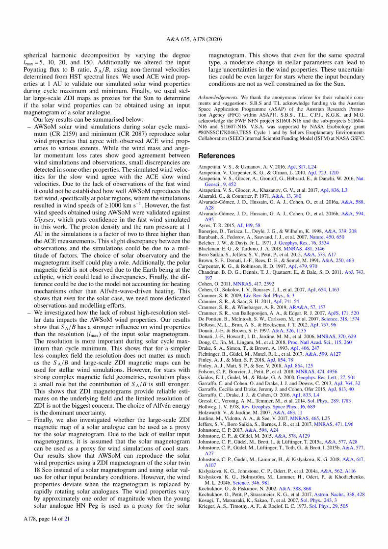
The two 4× 4 grids of simulations were created by altering thetwo key input parameters lmax and S A/B. The S A/B value of1.1× 106 W m−2 T−1 is the solar S A/B taken from Sokolov et al.(2013). The other three values of S A/B were determined fromthe HST spectra of 18 Sco. The other input parameters listed inTable 1 were kept constant. The two grids represent solar cyclemaximum (CR 2159) and minimum (CR 2087).

Figure 9 shows the mass loss rate for our two 4× 4 grids.During solar cycle maximum (left panel of Fig. 9), the massloss rate changes by a factor of 61.5 over a range of lmaxfor a given S A/B. For example, keeping S A/B constant at1.1× 106 W m−2 T−1 and only changing the lmax, the differ-ence in the mass loss rate between the four simulations is afactor of about 1.5. However, if we keep lmax constant and usedifferent values of S A/B, the mass loss rate can differ by a fac-tor approximately 3. For the set of simulations where lmax = 5,the mass loss rate changes by a factor of 2.6 over a range ofS A/B. During solar cycle minimum (Fig. 9, right), the massloss rate shows almost no variability for different values of lmaxat a constant S A/B. The mass loss rate changes by a factor ofabout 2.7 or less for simulations with a constant lmax and varyingS A/B.

Our results show that, depending on the activity level of theSun, the resolution (lmax) of the magnetic map has a small or neg-ligible influence on the mass flux. During solar cycle maximum,the mass loss rate has a stronger dependence on the resolution(Table F.1) than during solar cycle minimum. Almost no vari-ation is detected in the simulated mass loss rates during solarcycle minimum (Table F.2). The mass flux has a much strongerdependence on the S A/B instead of lmax. Irrespective of the solaractivity cycle, the mass loss rate changes by a factor of betweentwo and three over a range of S A/B at a given lmax.

The angular momentum loss rate for the two grids duringsolar cycle maximum and minimum are shown in Fig. 10. Thevariability in angular momentum loss for different values of lmaxat a constant S A/B during cycle maximum is a factor of 61.5.The variability increases to a factor of about 2 for different val-ues of S A/B at a constant lmax (Table F.1). During solar cycleminimum, the angular momentum shows negligible variationsover a range of lmax at a constant S A/B; it varies by a factor of6 1.9 over a range of S A/B at a constant lmax. The angularmomentum loss shows similar dependence on lmax and S A/B tothe mass loss rate. Tables F.1 and F.2 show the mass loss andthe angular momentum loss rates for the two grids during cyclemaximum and minimum respectively.

The mass loss and angular momentum loss rates show aslight decrease as the resolution lowers, as shown in Figs. 9and 10. This could be attributed to the loss of small-scale mag-netic features for low values of lmax, resulting in a simpler fieldgeometry. According to Wang & Sheeley (1990), the expansionof flux tubes from the photosphere to the corona determinesthe wind density, temperature, velocity, and mass flux. Thehigher the expansion factor, the stronger the wind mass loss rate.The expansion factor increases for small-scale features which isanother explanation for stronger mass loss rates for higher valuesof lmax. Furthermore, higher lmax also leads to stronger surface

A178, page 10 of 21

S. Boro Saikia et al.: Solar wind

Table 4. Median and mean values of the wind speed, proton density, and ram pressure for the slow and the fast wind of both AWSoM simulations(lmax = 150 and S A/B = 1.1× 106 W m−2 T−1) and ACE observations.

Median ur Mean ur Median np Mean np Median Pram Mean Pram

[km s−1] [km s−1] [cm−3] [cm−3] [nPa] [nPa]

Slow windAWSoM 391 380 12.7 20.3 31.8 35.3

ACE 420 430 4.0 5.1 12.4 15.0

Fast windAWSoM 794 790 2.1 2.2 22.3 23.0

ACE 639 647 2.3 3.2 17.2 21.9

Fig. 9. Mass loss rate for the grid of simulations during cycle maximum (CR 2159) (left) and minimum (CR 2087) (right). The different coloursrepresent different values of lmax.

Fig. 10. Same as Fig. 9 except the angular momentum loss rate is shown instead of the mass loss rate.

magnetic field, which leads to higher heating at the base leadingto more mass loss. The higher expansion factor during solar cyclemaximum, when the number of small-scale features is higher,could also explain the increase in mass loss rate for CR 2159.

The impact of stellar magnetogram resolution was also inves-tigated by Jardine et al. (2017), who lowered the resolution ofsolar magnetograms using the same method as used in this work

and used an empirical wind model to establish that the massand angular momentum loss rates for a low-resolution magne-togram are within 5–20% of the full resolution value. Since thelarge-scale dipole field is the key driver of mass and angularmomentum loss in Sun-like stars, the resolution loss in ZDI doesnot have a significant influence on the mass or angular momen-tum loss rates (Réville et al. 2015; See et al. 2018). However, the

A178, page 11 of 21

A&A 635, A178 (2020)

Fig. 11. Solar mass loss rate for different ZDI input magnetograms, shown in magenta, as a function of rotation period (left) and dipolar fieldstrength in Gauss (right). Solar symbols connected by the black vertical line shows the mass loss rate for the solar input magnetograms (lmax = 10)during solar cycle minimum and maximum.

resolution of the magnetogram might have a stronger impact forslowly rotating stars with Rossby number 2 (See et al. 2019).

Surprisingly, lmax = 20 leads to a marginally higher mass lossand angular momentum loss rate when compared to lmax = 150during solar cycle maximum in CR 2159. As lmax = 150 hasmore closed small-scale magnetic regions it is expected to havethe strongest mass and angular momentum loss. As shown inEq. (9), M depends on the wind velocity ur and density ρ. As thesolar wind moves outwards, the velocity increases and the num-ber density decreases. Figure C.1 shows that during solar cyclemaximum, the number density is slightly higher for lmax = 20compared to lmax = 150. This could explain the slightly highermass loss rate for lmax = 20.

The S A/B has a stronger influence on the wind mass lossand stellar angular momentum loss compared to the choice oflmax. This is not surprising since the Alfvén wave energy deter-mines the heating and acceleration of the wind in the AWSoMmodel. This shows that robust determination of S A/B is impor-tant for strong magnetic fields with complex field geometries.Our results also show that the O IV line is a good tracer for S A/Bscaling. However, further investigations are needed to determineits suitability for other stars.

As the variation in mass loss and angular momentum lossis not significant over the given range of lmax, we investigatedhow the wind speed, proton number density, and ram pressureare affected for the different values of S A/B in Table 2. Weused the lowest (lmax = 5) and the highest (lmax = 150) resolutionmagnetograms for this purpose. These three wind properties forthe fast and slow wind are determined from the combined solarmaximum and minimum simulations.

Figure D.1 shows the wind speed for different values ofS A/B at lmax = 150 (upper panel) and lmax = 5 (lower panel),respectively. As expected, the distribution of the wind velocityis almost consistent for the high-resolution (lmax = 150) and thelow-resolution (lmax = 5) simulations. The wind velocity showsa considerable variation with a varying S A/B. As the S A/Bincreases the wind velocity of the fast wind decreases, whilethe slow component does not show any considerable change inwind speeds. Tables F.3 and F.4 show the median and meanwind velocities at a distance of 1 AU for the distributions shownin Fig. D.1. The proton density distribution of the slow andfast wind for lmax = 150 and 5 over a varying S A/B is shown

in Figs. D.2 and D.3, respectively. The proton density for bothslow fast wind increases with increasing S A/B. The densityincreases by a factor of approximately two from S A/B = 1.2–2.2.The median and mean values are shown in Tables F.3 and F.4.The ram pressure shows a similar trend to the proton densitydistribution, as shown in Figs. D.4 and D.5; it also shows a vari-ation by a factor of approximately two depending on the choiceof S A/B. Although the mean and median wind velocity are notstrongly influenced by the choice of S A/B, the density varies bya factor of about two, resulting in a corresponding change in rampressure. The median and mean values of the ram pressure aretabulated in Tables F.3 and F.4. Our results show that, similarto the mass loss and angular momentum loss rates, the densityand ram pressure are more influenced by the S A/B than by theresolution. Although the mean and median wind velocities arenot strongly impacted by the variation of either S A/B or lmax, thedistribution of the fast wind shows some dependence on S A/B.For the solar case the variation is a factor of between two andthree, but it could be much higher for a more active star.

4.3. Solar wind properties determined using ZDI stellarmagnetograms

One problem often faced in stellar wind modelling is the lackof stellar magnetograms, as ZDI stellar magnetic maps are onlyavailable for <100 stars. To circumvent this problem, solar mag-netograms are sometimes used as a proxy for the stellar magneticfield in stellar wind modelling (Dong et al. 2018). Unfortunatelyit is not known whether or not such approximations introduceany additional biases in the simulated wind properties. We inves-tigated if the solar wind properties can be reproduced if we useZDI magnetograms of Sun-like stars as the input for the solarmagnetic field. This will allow us to have some insight into theusability of a magnetic map from one star (or even the sun) fora study of the wind properties of another. We used large-scaleZDI magnetic maps of three solar analogues as a proxy for thesolar magnetogram to carry out AWSoM solar wind simulations.The ZDI maps were used instead of the GONG magnetogramsused in the previous section. Solar input boundary conditions areused, which are the same values as listed in Table 1. Figure E.1shows the velocity distribution of a steady-state simulation ofone of the solar proxies HN Peg.

A178, page 12 of 21

S. Boro Saikia et al.: Solar wind

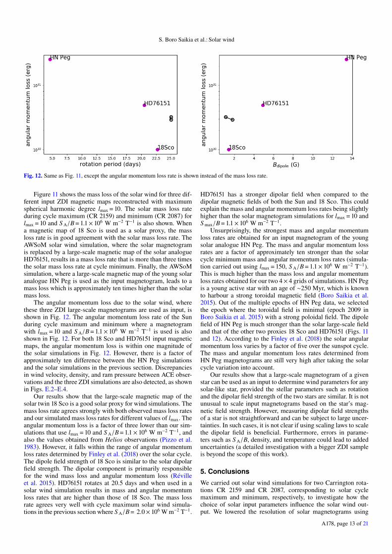
Fig. 12. Same as Fig. 11, except the angular momentum loss rate is shown instead of the mass loss rate.

Figure 11 shows the mass loss of the solar wind for three dif-ferent input ZDI magnetic maps reconstructed with maximumspherical harmonic degree lmax = 10. The solar mass loss rateduring cycle maximum (CR 2159) and minimum (CR 2087) forlmax = 10 and S A/B = 1.1× 106 W m−2 T−1 is also shown. Whena magnetic map of 18 Sco is used as a solar proxy, the massloss rate is in good agreement with the solar mass loss rate. TheAWSoM solar wind simulation, where the solar magnetogramis replaced by a large-scale magnetic map of the solar analogueHD76151, results in a mass loss rate that is more than three timesthe solar mass loss rate at cycle minimum. Finally, the AWSoMsimulation, where a large-scale magnetic map of the young solaranalogue HN Peg is used as the input magnetogram, leads to amass loss which is approximately ten times higher than the solarmass loss.

The angular momentum loss due to the solar wind, wherethese three ZDI large-scale magnetograms are used as input, isshown in Fig. 12. The angular momentum loss rate of the Sunduring cycle maximum and minimum where a magnetogramwith lmax = 10 and S A/B = 1.1× 106 W m−2 T−1 is used is alsoshown in Fig. 12. For both 18 Sco and HD76151 input magneticmaps, the angular momentum loss is within one magnitude ofthe solar simulations in Fig. 12. However, there is a factor ofapproximately ten difference between the HN Peg simulationsand the solar simulations in the previous section. Discrepanciesin wind velocity, density, and ram pressure between ACE obser-vations and the three ZDI simulations are also detected, as shownin Figs. E.2–E.4.

Our results show that the large-scale magnetic map of thesolar twin 18 Sco is a good solar proxy for wind simulations. Themass loss rate agrees strongly with both observed mass loss ratesand our simulated mass loss rates for different values of lmax. Theangular momentum loss is a factor of three lower than our sim-ulations that use lmax = 10 and S A/B = 1.1× 106 W m−2 T−1, andalso the values obtained from Helios observations (Pizzo et al.1983). However, it falls within the range of angular momentumloss rates determined by Finley et al. (2018) over the solar cycle.The dipole field strength of 18 Sco is similar to the solar dipolarfield strength. The dipolar component is primarily responsiblefor the wind mass loss and angular momentum loss (Révilleet al. 2015). HD76151 rotates at 20.5 days and when used in asolar wind simulation results in mass and angular momentumloss rates that are higher than those of 18 Sco. The mass lossrate agrees very well with cycle maximum solar wind simula-tions in the previous section where S A/B = 2.0× 106 W m−2 T−1.

HD76151 has a stronger dipolar field when compared to thedipolar magnetic fields of both the Sun and 18 Sco. This couldexplain the mass and angular momentum loss rates being slightlyhigher than the solar magnetogram simulations for lmax = 10 andS max/B = 1.1× 106 W m−2 T−1.

Unsurprisingly, the strongest mass and angular momentumloss rates are obtained for an input magnetogram of the youngsolar analogue HN Peg. The mass and angular momentum lossrates are a factor of approximately ten stronger than the solarcycle minimum mass and angular momentum loss rates (simula-tion carried out using lmax = 150, S A/B = 1.1× 106 W m−2 T−1).This is much higher than the mass loss and angular momentumloss rates obtained for our two 4× 4 grids of simulations. HN Pegis a young active star with an age of ∼250 Myr, which is knownto harbour a strong toroidal magnetic field (Boro Saikia et al.2015). Out of the multiple epochs of HN Peg data, we selectedthe epoch where the toroidal field is minimal (epoch 2009 inBoro Saikia et al. 2015) with a strong poloidal field. The dipolefield of HN Peg is much stronger than the solar large-scale fieldand that of the other two proxies 18 Sco and HD76151 (Figs. 11and 12). According to the Finley et al. (2018) the solar angularmomentum loss varies by a factor of five over the sunspot cycle.The mass and angular momentum loss rates determined fromHN Peg magnetograms are still very high after taking the solarcycle variation into account.

Our results show that a large-scale magnetogram of a givenstar can be used as an input to determine wind parameters for anysolar-like star, provided the stellar parameters such as rotationand the dipolar field strength of the two stars are similar. It is notunusual to scale input magnetograms based on the star’s mag-netic field strength. However, measuring dipolar field strengthsof a star is not straightforward and can be subject to large uncer-tainties. In such cases, it is not clear if using scaling laws to scalethe dipolar field is beneficial. Furthermore, errors in parame-ters such as S A/B, density, and temperature could lead to addeduncertainties (a detailed investigation with a bigger ZDI sampleis beyond the scope of this work).

5. Conclusions

We carried out solar wind simulations for two Carrington rota-tions CR 2159 and CR 2087, corresponding to solar cyclemaximum and minimum, respectively, to investigate how thechoice of solar input parameters influence the solar wind out-put. We lowered the resolution of solar magnetograms using

A178, page 13 of 21

A&A 635, A178 (2020)

spherical harmonic decomposition by varying the degreelmax = 5, 10, 20, and 150. Additionally we altered the inputPoynting flux to B ratio, S A/B, using non-thermal velocitiesdetermined from HST spectral lines. We used ACE wind prop-erties at 1 AU to validate our simulated solar wind propertiesduring cycle maximum and minimum. Finally, we used stel-lar large-scale ZDI maps as proxies for the Sun to determineif the solar wind properties can be obtained using an inputmagnetogram of a solar analogue.

Our key results can be summarised below:– AWSoM solar wind simulations during solar cycle maxi-

mum (CR 2159) and minimum (CR 2087) reproduce solarwind properties that agree with observed ACE wind prop-erties to various extents. While the wind mass and angu-lar momentum loss rates show good agreement betweenwind simulations and observations, small discrepancies aredetected in some other properties. The simulated wind veloc-ities for the slow wind agree with the ACE slow windvelocities. Due to the lack of observations of the fast windit could not be established how well AWSoM reproduces thefast wind, specifically at polar regions, where the simulationsresulted in wind speeds of ≥1000 km s−1. However, the fastwind speeds obtained using AWSoM were validated againstUlysses, which puts confidence in the fast wind simulatedin this work. The proton density and the ram pressure at 1AU in the simulations is a factor of two to three higher thanthe ACE measurements. This slight discrepancy between theobservations and the simulations could be due to a mul-titude of factors. The choice of solar observatory and themagnetogram itself could play a role. Additionally, the polarmagnetic field is not observed due to the Earth being at theecliptic, which could lead to discrepancies. Finally, the dif-ference could be due to the model not accounting for heatingmechanisms other than Alfvén-wave-driven heating. Thisshows that even for the solar case, we need more dedicatedobservations and modelling efforts.

– We investigated how the lack of robust high-resolution stel-lar data impacts the AWSoM wind properties. Our resultsshow that S A/B has a stronger influence on wind propertiesthan the resolution (lmax) of the input solar magnetogram.The resolution is more important during solar cycle max-imum than cycle minimum. This shows that for a simplerless complex field the resolution does not matter as muchas the S A/B and large-scale ZDI magnetic maps can beused for stellar wind simulations. However, for stars withstrong complex magnetic field geometries, resolution playsa small role but the contribution of S A/B is still stronger.This shows that ZDI magnetograms provide reliable esti-mates on the underlying field and the limited resolution ofZDI is not the biggest concern. The choice of Alfvén energyis the dominant uncertainty.

– Finally, we also investigated whether the large-scale ZDImagnetic map of a solar analogue can be used as a proxyfor the solar magnetogram. Due to the lack of stellar inputmagnetograms, it is assumed that the solar magnetogramcan be used as a proxy for wind simulations of cool stars.Our results show that AWSoM can reproduce the solarwind properties using a ZDI magnetogram of the solar twin18 Sco instead of a solar magnetogram and using solar val-ues for other input boundary conditions. However, the windproperties deviate when the magnetogram is replaced byrapidly rotating solar analogues. The wind properties varyby approximately one order of magnitude when the youngsolar analogue HN Peg is used as a proxy for the solar

magnetogram. This shows that even for the same spectraltype, a moderate change in stellar parameters can lead tolarge uncertainties in the wind properties. These uncertain-ties could be even larger for stars where the input boundaryconditions are not as well constrained as for the Sun.

Acknowledgements. We thank the anonymous referee for their valuable com-ments and suggestions. S.B.S and T.L acknowledge funding via the AustrianSpace Application Programme (ASAP) of the Austrian Research Promo-tion Agency (FFG) within ASAP11. S.B.S., T.L., C.P.J., K.G.K. and M.G.acknowledge the FWF NFN project S11601-N16 and the sub-projects S11604-N16 and S11607-N16. V.S.A. was supported by NASA Exobiology grant#80NSSC17K0463,TESS Cycle 1 and by Sellers Exoplanetary EnvironmentsCollaboration (SEEC) Internal Scientist Funding Model (ISFM) at NASA GSFC.

ReferencesAirapetian, V. S., & Usmanov, A. V. 2016, ApJ, 817, L24Airapetian, V., Carpenter, K. G., & Ofman, L. 2010, ApJ, 723, 1210Airapetian, V. S., Glocer, A., Gronoff, G., Hébrard, E., & Danchi, W. 2016, Nat.

Geosci., 9, 452Airapetian, V. S., Glocer, A., Khazanov, G. V., et al. 2017, ApJ, 836, L3Alazraki, G., & Couturier, P. 1971, A&A, 13, 380Alvarado-Gómez, J. D., Hussain, G. A. J., Cohen, O., et al. 2016a, A&A, 588,

A28Alvarado-Gómez, J. D., Hussain, G. A. J., Cohen, O., et al. 2016b, A&A, 594,

A95Ayres, T. R. 2015, AJ, 149, 58Banerjee, D., Teriaca, L., Doyle, J. G., & Wilhelm, K. 1998, A&A, 339, 208Barabash, S., Fedorov, A., Sauvaud, J. J., et al. 2007, Nature, 450, 650Belcher, J. W., & Davis, Jr. L. 1971, J. Geophys. Res., 76, 3534Blackman, E. G., & Tarduno, J. A. 2018, MNRAS, 481, 5146Boro Saikia, S., Jeffers, S. V., Petit, P., et al. 2015, A&A, 573, A17Brown, S. F., Donati, J.-F., Rees, D. E., & Semel, M. 1991, A&A, 250, 463Carpenter, K. G., & Robinson, R. D. 1997, ApJ, 479, 970Chandran, B. D. G., Dennis, T. J., Quataert, E., & Bale, S. D. 2011, ApJ, 743,

197Cohen, O. 2011, MNRAS, 417, 2592Cohen, O., Sokolov, I. V., Roussev, I. I., et al. 2007, ApJ, 654, L163Cranmer, S. R. 2009, Liv. Rev. Sol. Phys., 6, 3Cranmer, S. R., & Saar, S. H. 2011, ApJ, 741, 54Cranmer, S. R., & Winebarger, A. R. 2019, ARA&A, 57, 157Cranmer, S. R., van Ballegooijen, A. A., & Edgar, R. J. 2007, ApJS, 171, 520De Pontieu, B., McIntosh, S. W., Carlsson, M., et al. 2007, Science, 318, 1574DeRosa, M. L., Brun, A. S., & Hoeksema, J. T. 2012, ApJ, 757, 96Donati, J.-F., & Brown, S. F. 1997, A&A, 326, 1135Donati, J.-F., Howarth, I. D., Jardine, M. M., et al. 2006, MNRAS, 370, 629Dong, C., Jin, M., Lingam, M., et al. 2018, Proc. Natl Acad. Sci., 115, 260Drake, S. A., Simon, T., & Brown, A. 1993, ApJ, 406, 247Fichtinger, B., Güdel, M., Mutel, R. L., et al. 2017, A&A, 599, A127Finley, A. J., & Matt, S. P. 2018, ApJ, 854, 78Finley, A. J., Matt, S. P., & See, V. 2018, ApJ, 864, 125Folsom, C. P., Bouvier, J., Petit, P., et al. 2018, MNRAS, 474, 4956Gaidos, E. J., Güdel, M., & Blake, G. A. 2000, Geophys. Res. Lett., 27, 501Garraffo, C. and Cohen, O. and Drake, J. J. and Downs, C. 2013, ApJ, 764, 32Garraffo, Cecilia and Drake, Jeremy J. and Cohen, Ofer 2015, ApJ, 813, 40Garraffo, C., Drake, J. J., & Cohen, O. 2016, ApJ, 833, L4Gressl, C., Veronig, A. M., Temmer, M., et al. 2014, Sol. Phys., 289, 1783Hollweg, J. V. 1978, Rev. Geophys. Space Phys., 16, 689Holzwarth, V., & Jardine, M. 2007, A&A, 463, 11Jardine, M., Vidotto, A. A., & See, V. 2017, MNRAS, 465, L25Jeffers, S. V., Boro Saikia, S., Barnes, J. R., et al. 2017, MNRAS, 471, L96Johnstone, C. P. 2017, A&A, 598, A24Johnstone, C. P., & Güdel, M. 2015, A&A, 578, A129Johnstone, C. P., Güdel, M., Brott, I., & Lüftinger, T. 2015a, A&A, 577, A28Johnstone, C. P., Güdel, M., Lüftinger, T., Toth, G., & Brott, I. 2015b, A&A, 577,

A27Johnstone, C. P., Güdel, M., Lammer, H., & Kislyakova, K. G. 2018, A&A, 617,

A107Kislyakova, K. G., Johnstone, C. P., Odert, P., et al. 2014a, A&A, 562, A116Kislyakova, K. G., Holmström, M., Lammer, H., Odert, P., & Khodachenko,

M. L. 2014b, Science, 346, 981Kochukhov, O., & Piskunov, N. 2002, A&A, 388, 868Kochukhov, O., Petit, P., Strassmeier, K. G., et al. 2017, Astron. Nachr., 338, 428Kosugi, T., Matsuzaki, K., Sakao, T., et al. 2007, Sol. Phys., 243, 3Krieger, A. S., Timothy, A. F., & Roelof, E. C. 1973, Sol. Phys., 29, 505

A178, page 14 of 21

S. Boro Saikia et al.: Solar wind

Lichtenegger, H. I. M., Lammer, H., Grießmeier, J.-M., et al. 2010, Icarus, 210,1

Lundin, R. 2011, Space Sci. Rev., 162, 309Matsumoto, T., & Suzuki, T. K. 2012, ApJ, 749, 8Matt, S. P., Brun, A. S., Baraffe, I., Bouvier, J., & Chabrier, G. 2015, ApJ, 799,

L23Matthaeus, W. H., Zank, G. P., Oughton, S., Mullan, D. J., & Dmitruk, P. 1999,

ApJ, 523, L93McComas, D. J., Bame, S. J., Barker, P., et al. 1998, Space Sci. Rev., 86, 563McComas, D. J., Elliott, H. A., Schwadron, N. A., et al. 2003,

Geophys. Res. Lett., 30, 1517McIntosh, S. W., de Pontieu, B., Carlsson, M., et al. 2011, Nature, 475, 477Nicholson, B. A., Vidotto, A. A., Mengel, M., et al. 2016, MNRAS, 459, 1907Ó Fionnagáin, D., Vidotto, A. A., Petit, P., et al. 2019, MNRAS, 483, 873Oran, R., van der Holst, B., Landi, E., et al. 2013, ApJ, 778, 176Oran, R., Landi, E., van der Holst, B., Sokolov, I. V., & Gombosi, T. I. 2017, ApJ,

845, 98Pagano, I., Linsky, J. L., Valenti, J., & Duncan, D. K. 2004, A&A, 415, 331Parker, E. N. 1958, ApJ, 128, 664Parker, E. N. 1965, Space Sci. Rev., 4, 666Pesnell, W. D., Thompson, B. J., & Chamberlin, P. C. 2012, Sol. Phys., 275, 3Peter, H. 2006, A&A, 449, 759Petit, P., Dintrans, B., Solanki, S. K., et al. 2008, MNRAS, 388, 80Petit, P., Louge, T., Théado, S., et al. 2014, PASP, 126, 469Pevtsov, A. A., Fisher, G. H., Acton, L. W., et al. 2003, ApJ, 598, 1387Phillips, K. J. H., Feldman, U., & Landi, E. 2008, Ultraviolet and X-ray

Spectroscopy of the Solar Atmosphere (Cambridge: Cambridge UniversityPress)

Piskunov, N., & Kochukhov, O. 2002, A&A, 381, 736Pizzo, V., Schwenn, R., Marsch, E., et al. 1983, ApJ, 271, 335Porto de Mello, G. F., & da Silva, L. 1997, ApJ, 482, L89Powell, K. G., Roe, P. L., Linde, T. J., Gombosi, T. I., & De Zeeuw, D. L. 1999,

J. Comput. Phys., 154, 284Réville, V., & Brun, A. S. 2017, ApJ, 850, 45Réville, V., Brun, A. S., Strugarek, A., et al. 2015, ApJ, 814, 99Riley, P., Ben-Nun, M., Linker, J. A., et al. 2014, Sol. Phys., 289, 769Robinson, R. D., Carpenter, K. G., & Brown, A. E. 1998, ApJ, 503, 396Rosén, L., Kochukhov, O., Hackman, T., & Lehtinen, J. 2016, A&A, 593,

A35

Sachdeva, N., van der Holst, B., Manchester, W. B., et al. 2019, ApJ, 887, 83See, V., Jardine, M., Vidotto, A. A., et al. 2018, MNRAS, 474, 536See, V., Matt, S. P., Finley, A. J., et al. 2019, ApJ, 886, 120Semel, M. 1989, A&A, 225, 456Sokolov, I. V., van der Holst, B., Oran, R., et al. 2013, ApJ, 764, 23Spitzer, L. 1956, Physics of Fully Ionized Gases (North Chelmsford, MA, USA:

Courier Corporation)Stone, E. C., Frandsen, A. M., Mewaldt, R. A., et al. 1998, Space Sci. Rev., 86, 1Suzuki, T. K. & Inutsuka, S.-I. 2006, J. Geophys. Res., 111, A06101Suzuki, T. K., Imada, S., Kataoka, R., et al. 2013, PASJ, 65, 98Tarduno, J. A., Cottrell, R. D., Watkeys, M. K., et al. 2010, Science, 327, 1238Tian, F., Kasting, J. F., Liu, H.-L., & Roble, R. G. 2008, J. Geophys. Res., 113,

E05008Tóth, G., van der Holst, B., & Huang, Z. 2011, ApJ, 732, 102Tóth, G., van der Holst, B., Sokolov, I. V., et al. 2012, J. Comput. Phys., 231, 870Usmanov, A. V., Goldstein, M. L., Besser, B. P., & Fritzer, J. M. 2000,

J. Geophys. Res., 105, 12675Usmanov, A. V., Matthaeus, W. H., Goldstein, M. L., & Chhiber, R. 2018, ApJ,

865, 25Valenti, J. A., & Fischer, D. A. 2005, ApJS, 159, 141van den Oord, G. H. J., & Doyle, J. G. 1997, A&A, 319, 578van der Holst, B., Jacobs, C., & Poedts, S. 2007, ApJ, 671, L77van der Holst, B., Sokolov, I. V., Meng, X., et al. 2014, ApJ, 782, 81Vidotto, A. A. 2016, MNRAS, 459, 1533Vidotto, A. A., & Bourrier, V. 2017, MNRAS, 470, 4026Vidotto, A. A., Jardine, M., Opher, M., Donati, J. F., & Gombosi, T. I. 2011,

MNRAS, 412, 351Vidotto, A. A., Jardine, M., Morin, J., et al. 2014, MNRAS, 438, 1162Villadsen, J., Hallinan, G., Bourke, S., Güdel, M., & Rupen, M. 2014, ApJ, 788,

112Wang, Y.-M., & Sheeley, Jr. N. R. 1990, ApJ, 355, 726Wargelin, B. J., & Drake, J. J. 2002, ApJ, 578, 503Weber, E. J., & Davis, Jr. L. 1967, ApJ, 148, 217Wood, B. E. 2004, Liv. Rev. Sol. Phys., 1, 2Wood, B. E., Linsky, J. L., & Ayres, T. R. 1997, ApJ, 478, 745Wood, B. E., Linsky, J. L., Müller, H.-R., & Zank, G. P. 2001, ApJ, 547, L49Wood, B. E., Müller, H.-R., Zank, G. P., & Linsky, J. L. 2002, ApJ, 574, 412Wood, B. E., Müller, H.-R., Zank, G. P., Linsky, J. L., & Redfield, S. 2005, ApJ,

628, L143

A178, page 15 of 21

A&A 635, A178 (2020)

Appendix A: Gaussian fit

Fig. A.1. Double Gaussian fit of the Si IV line at 1393.75 Å.

Appendix B: Mass and angular momentum lossrates versus distance

Fig. B.1. Mass loss (top) and angular momentum loss (bottom) rates areshown as a function of radius for both solar maximum (CR 2159, black)and solar minimum case (CR 2087, red).

A178, page 16 of 21

S. Boro Saikia et al.: Solar wind

Appendix C: Number density versus velocity ur

Fig. C.1. Proton number density vs. wind velocity, ur during solar maximum, CR 2159. The lmax = 150 simulation is shown in magenta and lmax = 20simulation output is shown in green.

Appendix D: Solar wind speed, proton density, and ram pressure for lmax = 150 and 5 over the givenrange of SA/B

Fig. D.1. Distribution of wind velocity at 1 AU for a subset of our simulations during solar cycle minimum and maximum. Each column representsa steady state simulation for different values of S A/B. The resolution of the magnetogram is truncated to lmax = 150 (top) and lmax = 5 (bottom). ACEdata is shown in green.

A178, page 17 of 21

A&A 635, A178 (2020)

Fig. D.2. Proton number density of the slow wind for the same simulations as in Fig . D.1. The observed ACE proton densities are shown in green.

Fig. D.3. Same as in Fig. D.2 but for the fast wind.

Fig. D.4. Ram pressure for the same simulations as in Fig. D.1. ACE ram pressure is shown in green.

A178, page 18 of 21

S. Boro Saikia et al.: Solar wind

Fig. D.5. Same as in Fig. D.4 but for the fast wind.

Appendix E: ZDI solar simulations

Fig. E.1. Same as Fig. 4 but for HN Peg.

Fig. E.2. Wind velocity determined from ZDI simulations of the three stars: 18 Sco, HD 76151, HN Peg (left to right) in magenta. The observedACE wind velocities are shown in green.

A178, page 19 of 21

A&A 635, A178 (2020)

Fig. E.3. Proton number density for the slow (top) and fast (bottom) component of the wind. Each column represents wind simulations for the threestars included in this work: 18 Sco, HD76151, HN Peg (left to right, magenta). ACE proton density is shown in green.

Fig. E.4. Same as in Fig. E.3 except the ram pressure is shown instead of the proton density.

A178, page 20 of 21

S. Boro Saikia et al.: Solar wind

Appendix F: Additional tables

Table F.1. Mass loss and angular momentum loss rates during solar cycle maximum (CR 2159) for different values of lmax and S A/B ×106 W m−2 T−1 in the grid.

M, × 10−14 M� yr−1 J, × 1030 ergS A/B = 1.1 S A/B = 1.2 S A/B = 2.0 S A/B = 2.2 S A/B = 1.1 S A/B = 1.2 S A/B = 2.0 S A/B = 2.2

lmax = 5 2.9 3.2 6.7 7.7 2.8 2.9 4.8 5.4lmax = 10 3.4 3.8 8.2 9.6 3.2 3.5 6.0 6.8lmax = 20 4.4 4.2 8.9 10.3 4.2 3.7 7.0 8.0

lmax = 150 4.1 3.9 8.4 9.7 4.0 3.7 6.5 7.3

Table F.2. Same as Table F.1 but during solar minimum (CR 2087).

M, × 10−14 M� yr−1 J, × 1030 ergS A/B = 1.1 S A/B = 1.2 S A/B = 2.0 S A/B = 2.2 S A/B = 1.1 S A/B = 1.2 S A/B = 2.0 S A/B = 2.2

lmax = 5 1.7 2.1 4.0 4.6 2.4 2.5 4.1 4.5lmax = 10 1.8 2.0 4.1 4.7 3.0 2.7 4.2 4.6lmax = 20 2.0 2.0 4.1 4.7 3.0 2.6 4.2 4.7

lmax = 150 2.1 2.1 4.2 4.9 3.0 2.8 4.3 4.7

Table F.3. Median and mean values of the wind speed, proton density, and ram pressure for the slow and the fast wind for simulations wherelmax = 150, and S A/B is determined from FUV spectra.

S A/B Median ur Mean ur Median np Mean np Median Pram Mean Pram

×106 W m−2 T−1 km s−1 km s−1 cm−3 cm−3 nPa nPa

Slow wind1.2 392 377 13.9 22.6 34.1 38.12.0 375 362 26.7 47.6 60.2 69.02.2 372 361 30.9 54.7 69.2 78.1

Fast wind1.2 781 776 2.4 2.5 24.3 24.92.0 703 701 5.9 5.9 48.4 48.42.2 692 692 6.9 7.0 60.0 55.8

Table F.4. Median and mean values of the wind speed, proton density, and ram pressure for the slow and the fast wind for simulations wherelmax = 5, and S A/B is determined from FUV spectra.

S A/B Median ur Mean ur Median np Mean np Median Pram Mean Pram

×106 W m−2 T−1 km s−1 km s−1 cm−3 cm−3 nPa nPa

Slow wind1.2 423 406 12.4 17.8 34.8 37.32.0 426 408 23.7 32.6 62.6 70.32.2 427 410 26.6 37.5 70.9 80.6

Fast wind1.2 791 778 2.1 2.2 21.2 21.72.0 706 696 5.3 5.3 42.1 42.12.2 691 683 6.4 6.3 48.7 48.6

A178, page 21 of 21