Ann. Geophys., 29, 2317–2326, 2011www.ann-geophys.net/29/2317/2011/doi:10.5194/angeo-29-2317-2011© Author(s) 2011. CC Attribution 3.0 License.

AnnalesGeophysicae

Relative ordering in the radial evolution of solar wind turbulence:the S-Theorem approach

G. Consolini1 and P. De Michelis2

1INAF – Istituto di Fisica dello Spazio Interplanetario, 00133 Roma, Italy2Istituto Nazionale di Geofisica e Vulcanologia, 00143 Roma, Italy

Received: 28 February 2011 – Revised: 4 November 2011 – Accepted: 21 November 2011 – Published: 23 December 2011

Abstract. Over the past few decades scientists have showngrowing interest in space plasma complexity and in under-standing the turbulence in magnetospheric and interplanetarymedia. At the beginning of the 1980s, Yu. L. Klimontovichintroduced a criterion, named S-Theorem, to evaluate the de-gree of order in far-from-equilibrium open systems, whichapplied to hydrodynamic turbulence showed that turbulenceflows were more organized than laminar ones. Using thesame theorem we have evaluated the variation of the degreeof self-organization in both Alfvenic and non-Alfvenic turbu-lent fluctuations with the radial evolution during a long timeinterval characterized by a slow solar wind. This analysisseems to show that the radial evolution of turbulent fluctu-ations is accompanied by a decrease in the degree of order,suggesting that, in the case of slow solar wind, the turbulencedecays with radial distance.

Keywords. Interplanetary physics (Solar wind plasma) –Space plasma physics (Turbulence)

1 Introduction

The solar wind results from the expansion of the solar at-mosphere, forming a supersonic flow of ionized plasma andmagnetic field that permeates the interplanetary medium. Itconsists mainly of protons and electrons with a small admix-ture of ionized helium and heavy ions. The solar magneticfield embedded in the plasma is a weak (a few nano Teslasnear the Earth) and is carried into space by the solar wind.Although the solar magnetic field is characterized by a com-plex structure on the Sun within less than 2 solar radii fromthe photosphere, in the solar wind it exhibits a simple ra-

Correspondence to:G. Consolini(giuseppe.consolini@ifsi-roma.inaf.it)

dially directed structure lying near the ecliptic plane in anArchimedean spiral pattern.

To treat the solar wind properly many approaches havebeen tried, each with a different approximation. Indeed, itis possible to study the solar wind using a fluid approxima-tion or a kinetic treatment; however, in both cases difficultiesexist (Russel, 2001). The result is that our understanding ofthe solar wind is nowadays founded on long term observa-tions rather than on solid theoretical foundations.

The solar wind was measured for the first time in the 1960swith the advent of spacecrafts. After the first measurements,it was clear that it was pervaded by fluctuations on a verywide range of scales. The subsequent studies of these fluc-tuations revealed a complex interaction among waves, tur-bulence and structures (see e.g.Bruno and Carbone, 2005).Nowadays, it is known that the solar wind is characterizedby the presence of fluctuations in the magnetic and veloc-ity fields that are often so highly correlated to appear asnearly perfect Alfven waves. The solar wind shows an activeturbulent cascade, which transfers energy from large scalesto small scales and heats the plasma (Verma et al., 1995;Marino et al., 2008). Finally, it exhibits a turbulence whichis anisotropic with respect to the magnetic field and it is alsocharacterized by intermittency similar to that found in neutralfluids.

Focusing on the turbulent nature of the solar wind, thepower spectrum of solar wind fluctuations provides one ofthe main evidences for the existence of an active turbulentcascade (Bruno and Carbone, 2005). Indeed, the power spec-trum of fluctuations of the magnetic field components, evalu-ated in the case of high speed solar wind, reveals broadbandfluctuations over all measured scales. These fluctuations arecharacterized by a power law spectrum, which depends onthe frequency range: at low frequencies the power law ex-hibits a spectral index near 1 while at higher frequencies thespectral index is near 5/3. The presence of a broad rangeof scales with anf −5/3 spectrum may be associated with a

Published by Copernicus Publications on behalf of the European Geosciences Union.

2318 G. Consolini and P. De Michelis: S-Theorem and solar wind turbulence radial evolution

turbulent cascade, being 5/3 the familiar value of the spectralindex in hydrodynamic turbulence. This turbulence followsfrom processes occurring in the solar wind and does not sim-ply reflect the nature of the solar wind emerging from thesolar corona. Indeed, according toBavassano et al.(1982a)the power spectrum of fluctuations changes its shape withdistance from the Sun, as the breakpoint between the tworegimesf −1 andf −5/3 shifts to lower frequencies (i.e. largerscales) with the increase of solar distance. Thus, the fluctu-ation properties evolve with both time and radial distance.Together with changes in the power spectrum with distance,there is a decrease in the Alfvenicity character of the fluctua-tions (Roberts et al., 1987), which seems to be closely relatedto the turbulent evolution. These results characterize mainlythe fast solar wind. Conversely, the slow solar wind spectraare characterized by a spectral index near 5/3 over a widerange of scales. The broadbandf −5/3 spectrum associatedwith a generally low Alfvenicity (Tu et al., 1989) suggeststhat slow solar wind fluctuations represent fully developedturbulence. For this reason, the solar wind evolution cannotbe reduced to a simple solar wind expansion with the helio-centric distance, but it involves nonlinear interactions amongpropagating Alfvenic modes (Tu et al., 1984). It has beenshown that intermittency increases with radial distance, prob-ably due to a change in the anisotropy degree of the magneticfluctuations. However, contradictory results have been foundas regards the evolution of the anisotropy degree with radialdistance. For instance,Bavassano et al.(1982b) showed thatin high-speed streams the orthogonal component of the mag-netic field fluctuations became more dominant with the in-crease of the distance, whileHorbury et al.(1995) claimedthat turbulence was more isotropic at larger heliospheric dis-tances in the case of polar solar wind.

Besides turbulence an important aspect characterizingthe solar wind is the presence of coherent advected struc-tures, which can be imagined like flux tubes (Ness et al.,1966; McCracken and Ness, 1966; Mariani et al., 1973;Tu and Marsch, 1990, 1993; Bruno et al., 2001; Borovsky,2008). The presence of such non-Alfvenic coherent struc-tures, whose origin is not completely understood, becomesmore relevant with radial distance (Bruno et al., 2006).

Recently,Consolini(2010) examined the radial evolutionof magnetic field intensity fluctuations during a long timeinterval characterized by a slow solar wind. This analysishas been based on the S-Theorem byKlimontovich (1983)in order to examine the changes of the degree of order ofthe magnetic field intensity fluctuations at two heliosphericdistances. The preliminary results have pointed toward anincrease in the degree of order with radial distance, whichsuggests the formation of coherent structures during the ra-dial evolution of magnetic field intensity fluctuations.

Here, analyzing the same long time interval of slow solarwind investigated byConsolini (2010), we carry out an in-depth analysis of the relative degree of order of the turbulentfluctuation field. In detail, we investigate the changes in the

probability distribution functions (PDFs) of the total specificenergy of turbulent fluctuations on the time scale of 1 h withradial distance, demonstrating that the radial evolution of tur-bulent fluctuations is associated with a chaotization process.

The paper is organized as follows: in Sect. 2, we brieflydescribe the Klimontovich S-Theorem; in Sect. 3 we applysuch a theorem to our data and in Sect. 4 we discuss andsummarize our results.

2 Klimontovich’ S-Theorem: a brief introduction

In thermodynamics and statistical mechanics the state ofmaximum disorder corresponds to the equilibrium state fora given condition of the external parameters, as clearly statedby the principle of maximum entropy. Thus, any deviationfrom the equilibrium configuration is associated with a re-duction of entropy. This happens, for instance, in nonequilib-rium stationary states, where the degree of order can increasedue to the emergence of a spatial-temporal coherence. In-deed, in many nonequilibrium systems we assist to the emer-gence of correlations and self-organization that imply a re-duction of thephysical chaos(uncorrelated microscopic mo-tion). In this framework, a crucial importance assumes theknowledge of a method able to quantify the relative degreeof order in different open nonequilibrium states of the samesystem.

Over the last two decades the concept ofdynamic chaoshas gained a particular relevance in the framework of com-plex motions in relatively simple systems. Dynamic chaos,which is consequence of dynamic instabilities, has not to beconfused with physical chaos, which is related to the absenceof coherence in the motion of particles in a state of thermo-dynamic equilibrium according to the original definition byBoltzmann. Consequently, it would be interesting to havea criterium to estimate quantitatively if the dynamic chaos,emerging from dynamic instabilities, could or not lead tomore ordered configurations.

In 1983 Klimontovich (Klimontovich, 1983, 1995) pro-posed an entropy-based approach to measure the relativedegree of order between two different states in an opennonequilibrium system. This approach, formulated as a theo-rem, named theSelf-organization Theorem(S-Theorem), at-tempts to solve one of the main tasks of the statistical theoryof open systems, establishing a criterium capable of mea-suring the degree of self-organization of an open system ina nonequilibrium configuration. The aim of theS-Theoremis to distinguish between degradation and self-organizationin different nonequilibrium configurations of open systems,thus providing a quantitative measure of order with respectto physical chaos (equilibrium).

The starting point of theS-Theoremis the Boltzmann’sH-theorem, according to which the entropy variation3S

Ann. Geophys., 29, 2317–2326, 2011 www.ann-geophys.net/29/2317/2011/

G. Consolini and P. De Michelis: S-Theorem and solar wind turbulence radial evolution 2319

between an equilibrium state and a nonequilibrium one ina system with a fixed value of mean energy is

3S= S0−S(t) = κB

∫f (X,t)ln

f (X,t)

f0(X)dX ≥ 0 (1)

under the condition,

d3S

dt=

d

dt(S0−S(t)) ≤ 0, (2)

beingκB is the Boltzmann’s constant,S0 (f0(X)) andS(t)

(f (X,t)) the entropies (distribution functions) of the equi-librium and nonequilibrium states, respectively. This theo-rem states that a system with fixed mean energy evolves to-wards an increase of entropy, which reaches its maximum atthe equilibrium state. Based on the condition of fixed meanenergy the above relationship implies that the entropy differ-ence3S(t) acts as aLyapunov functionalfor the evolution ofa system.

However, the entropy reduction3S is inadequate to es-timate the relative degree of order in systems whose statesdepend on a control parameter that yields different mean en-ergy values. This is particularly true in the case of open sys-tems where the mean energy is generally not constant dur-ing the evolution. For these types of systems an appropriateLyapunov functional for the evolution is impossible to definecorrectly in terms of entropy difference. In other words, it isnot possible to evaluate the relative degree of order betweentwo open systems in different nonequilibrium states using theprevious relationship. Klimontovich’s S-Theorem finds a so-lution to this problem renormalizing the distribution of thereference state and making use of escort distributions. TheS-Theorem provides a measure of the degree of order rela-tive to a reference state for open systems, thereby supplyingthe correct ordering of entropy values with respect to theirdistance from the equilibrium state.

Given two different nonequilibrium states,A(a0) andA(a0 + δa), of the same open system, which correspond totwo different values (a0 anda0+δa) of a controlling param-eter, we indicate withf (X;a0) andf (X;a0 + δa) the cor-respondent time independent distribution functions for theobservableX based on the hypothesis ofstationary exter-nal conditions(i.e. a time-scale separation between fast pro-cesses and the slow background evolution). To take into ac-count the possible change of the mean energy it is necessaryto renormalizethe distribution function associated with oneof the two states, taken as thereference state, before evaluat-ing the entropy reduction (Klimontovich, 1995).

Thus, we assume as reference state (i.e. as the most chaoticstate) the one witha = a0 and identify withf0 ≡ f (X;a0) itsdistribution function, and withf1 ≡ (X;a0 + δa) the distri-bution function of the other state. Following Klimontovich’sprocedure, we introduce aneffective Hamiltonian or energyHeff(X;a0) as

Heff(X;a0) = −lnf0(X;a0). (3)

To ensure that the mean effective energy of the reference stateis equal to that associated with the other state, we have torenormalize the reference state distribution function as fol-lows,

f0(X;a0,δa)= exp

[Feff −Heff(X;a0)

Teff(δa)

], (4)

whereFeff is theeffective free energythat can be expressedin terms of theeffective temperatureTeff on the basis of thenormalization condition,∫

f0(X;a0,δa)dX = 1. (5)

It follows

Feff = −Teff ln∫

exp

(−

Heff(X;a0)

Teff

)dX. (6)

We remark that the effective Hamilton functionHeff is notrepresentative of the conventional concept of energy.

Based on the previous mathematical assumptions, the onlyfree parameter is the effective temperatureTeff(δa), whichcan be determined by imposing that the two distribution func-tions f0 andf1 have the same mean effective energy,∫

Hefff0(X;a0,δa)dX =

∫Hefff1(X;a0+δa)dX. (7)

Consequently, we have

Teff(δa) |δa=0= 1, (8)

where the conditionδa = 0 refers to the reference state.Once we have renormalized the reference state distribu-

tion function according to the condition of constant effectivemean energy, we obtain two distribution functionsf0 andf1,with the same mean energy. The entropy difference betweenthe two states can be evaluated using Eq. (1), i.e.

δS = S0−S =

∫f1ln

f1

f0dX, (9)

whereδS ≥ 0 if we made the right choice of the referencestate of physical chaos.

The solution of Eq. (7) provides a quantitative measureof the relative order between two selected states. Indeed, ifthe condition of Eq. (7) is satisfied forTeff(δa) > 1, we willhave to raise the effective temperature and add heat to thereference state “0” to modify it into the more organized state“1”. Thus, the state “0” is a state with more physical chaosthan the state “1”. To clarify the meaning of the effectivetemperatureTeff as a measure of the degree of order we in-vite the reader to consult the Appendix A where we make allthe above calculations in the case of a simple system. Wenote that the concept of state of maximum physical chaoshas to be associate with the equilibrium state, where accord-ing to Boltzmann the particle motion is chaotic and generallyuncorrelated. In other words, the term “physical chaos” is

www.ann-geophys.net/29/2317/2011/ Ann. Geophys., 29, 2317–2326, 2011

2320 G. Consolini and P. De Michelis: S-Theorem and solar wind turbulence radial evolution

800

600

400

200|v

x| [k

m/s

]

15-09-1997 15-11-1997 15-01-1998 15-03-1998

UT

1AU

500

450

400

350

300

250

v r [

km/s

]

15-09-1997 15-11-1997 15-01-1998 15-03-1998

UT

5AU

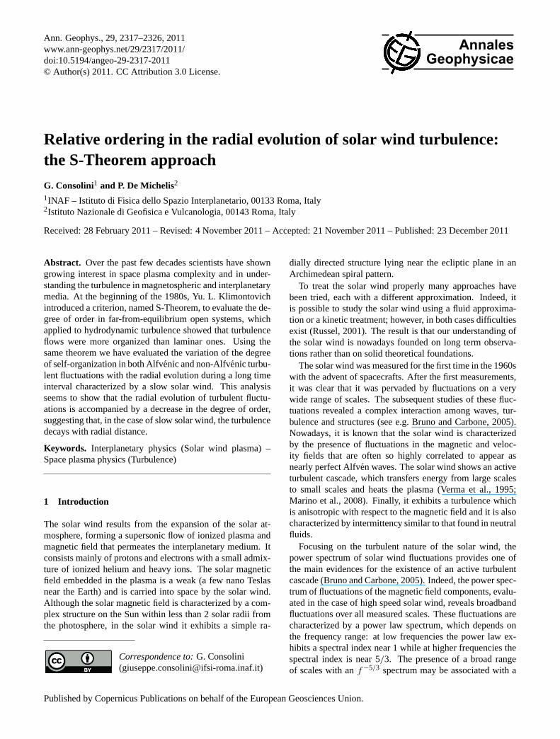
Fig. 1. The X-component of the solar wind velocity at 1 AU (upper panel) and the radial component of the solar wind velocity at 5 AU (lowerpanel) for the period from 1 September 1997 to 31 March 1998. Horizontal solid blue lines indicate mean values (blue line); dashed lineslimit ±1 standard deviation intervals.

directly connected with uncorrelated stochastic motions andnot with the sensitivity to initial conditions.

We emphasize that in nonequilibrium systems the emer-gence ofcomplexityanddynamical complexityis identifiedwith the tendency to manifest spatio-temporal coherent struc-tures and features. These generally result from the com-petition of different basic spatial patterns (Badii and Politi,1997), and require the intertwining of order and disorder(Nicolis and Nicolis, 2007). For instance, this happens inthe case of turbulence, where the turbulent eddies are coher-ent structures. On the other hand, the existence of coherentstructures in a system is the counterpart of a self-organizationprocess, which increases the coherence and the correlationin the system and reduces the degree of disorder or physi-cal chaos, i.e. uncorrelated motions. (Klimontovich, 1991,1996). Thus, it is reasonable to observe a significant reduc-tion of the degree of disorder in a complex system, in agree-ment with the S-theorem.

3 Data and results

To study the relative order and the occurrence of self-organization in the solar wind turbulence radial evolution weconsider the hourly variances of the interplanetary magneticand velocity fields measured in situ at 1 AU and at∼5 AU inthe time interval September 1997–March 1998. Data at 1 AUcome from the OMNI database (NSSDC-USA), while dataat∼5 AU come from theUlyssesmeasurements, available atNASA-CDAweb. Typical data time resolution is 1 min apartfrom Ulysses velocity which is at about 4–8 min.

The chosen period is a long-lasting time interval of quietsolar wind conditions, already investigated and discussed inprevious works (Consolini et al., 2008; Consolini, 2010).During this period the solar wind velocity is slow and moreor less constant with small gradients (see Fig.1). For thisreason, as a first approximation, we can assume that the so-lar wind conditions are quasi-stationary. The average veloc-ity is 〈vx〉 = [370± 60] km s−1 at 1 AU and〈vR〉 = [370±

20] km s−1 at 5 AU.Due to the absence of a long-lasting alignment between

the two observational points at 1 AU and 5 AU, we are notobserving the same solar wind, but the choice of such a longperiod will guarantee a statistical validity to our analysis. Totake account the approx. 20 days solar wind traveling timefrom 1 AU to 5 AU, we cut-off the last 20 days from the 1 AUdata and the first 20 days from the 5 AU data.

To analyze the evolution of the turbulent solar wind fea-tures with the radial distance, we evaluate the 1 h variances ofthe plasma velocity and solar wind magnetic field expressedin Alfv en units (B → B/

√4πρ with ρ plasma density), i.e.

〈v2〉1 h and〈b2

〉1 h, wherev = V −〈V 〉1 h andb = B−〈B〉1 h.We identify the total specific energyEt of the fluctuation

field with the dynamical variable capable of representing theturbulence level

Et = Ev +Eb. (10)

This dynamical variable takes into account of the kinetic (Ev)and magnetic (Eb) specific energies, defined as

Ev =1

2〈v2

〉1 h, (11)

Ann. Geophys., 29, 2317–2326, 2011 www.ann-geophys.net/29/2317/2011/

G. Consolini and P. De Michelis: S-Theorem and solar wind turbulence radial evolution 2321

-1.0

-0.5

0.0

0.5

1.0

σ r

-1.0 -0.5 0.0 0.5 1.0

σc

III

IIIIV10

0

101

102

103

104

Ev

[km

2 /s2 ]

100

101

102

103

104

Eb [km2/s

2]

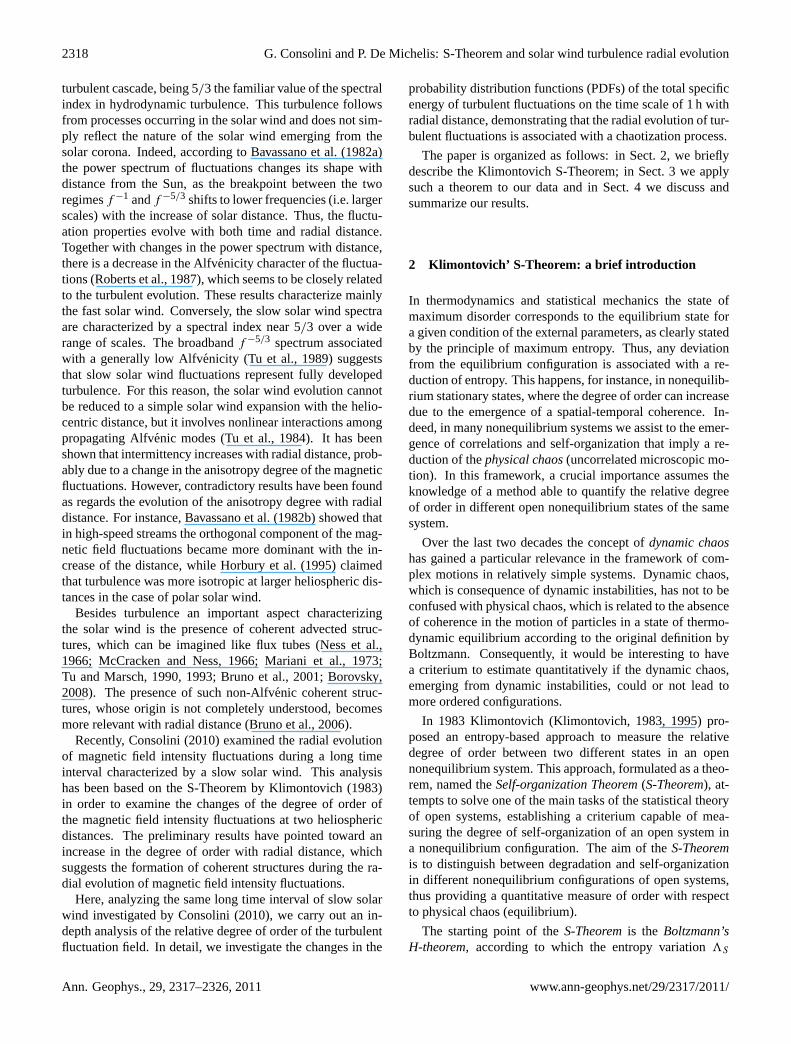
Fig. 2. The kinetic specific energyEv plotted versus the magnetic specific energyEb (left panel) and the scatter plot of the normalizedresidual energyσr versus the normalized cross-helicityσc (right panel) for the sample at 1 AU. The solid line in theEv −Eb plot refers tothe condition of complete equipartition.

-1.0

-0.5

0.0

0.5

1.0

σ r

-1.0 -0.5 0.0 0.5 1.0

σc

III

IIIIV0.1

1

10

100

1000

Ev

[km

2 /s2 ]

10-1

100

101

102

103

104

Eb [km2/s

2]

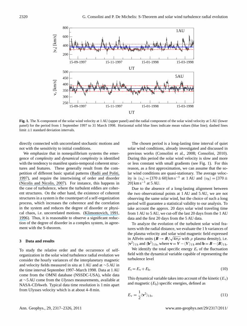
Fig. 3. The same of Fig.2 for the sample at 5 AU.

Eb =1

2〈b2

〉1 h. (12)

Furthermore to recognize theAlfvenicpart in the solar windfluctuations we compute thenormalized cross-helicityσc andthenormalized residual energyσr,

σc =2〈v ·b〉1 h

〈v2〉1 h+〈b2〉1 h, (13)

σr =Ev −Eb

Et. (14)

Here, the normalized cross-helicityσc, which can vary from−1 to +1, quantifies the degree of correlation between thevelocity and magnetic field fluctuations, expected to be maxi-mum for Alfvenic fluctuations, while the normalized residualenergy is a measure of the energy equipartition between thekinetic and magnetic fluctuations (Bavassano et al., 2000).

Figures2 and3 exhibit the kinetic specific energyEv as afunction of the magnetic specific energyEb and the normal-ized residual energyσr versus the normalized cross-helicityσc for both the data samples at 1 AU and 5 AU. The en-ergy equipartition is missed both at 1 AU and 5 AU. TheEb values are generally higher than the correspondingEvones. This result suggests that a significant part of the to-

tal energy of fluctuations comes from magnetic componentwhen a time scale of 1 h is considered. This is more ev-ident at 5 AU than at 1 AU. Indeed, the density of dots ishigher at 5 AU than at 1 AU in the IV quadrant of theσr −σcplane, and the mean value of the ratio betweenEv andEb ishigher at 1 AU (〈Ev/Eb〉1 AU = [0.70±0.02]) than at 5 AU(〈Ev/Eb〉5 AU = [0.64± 0.01]). Furthermore, according toFig. 3 the results relative toσc andσr well agree with pre-vious findings byConsolini et al.(2008), relative to a pre-dominance of magnetic fluctuations at 5 AU.

Now, we evaluate the probability distribution functions(PDFs) of the total specific energy (Et) at the two differ-ent solar distances and, as special cases, the PDFs rela-tive to Alfvenic and non-Alfvenic fluctuations. The selec-tion of Alfv enic/non-Alfvenic fluctuations is based onσr andσc values. For example, only data with 0.2≤| σc |≤ 1 and| σr |≤| σc | are considered for Alfvenic fluctuations, wherethe choice| σc |

min= 0.2, as the inferior limit of a significa-

tive normalized cross-correlation value, is based on 5 % null-hypothesys threshold for uncorrelated 3-D-vectors. In con-trast, those intervals where| σc |≤| σr | and 0.2≤| σr |≤ 1 arethe values used for the selection of non-Alvenic fluctuations.

www.ann-geophys.net/29/2317/2011/ Ann. Geophys., 29, 2317–2326, 2011

2322 G. Consolini and P. De Michelis: S-Theorem and solar wind turbulence radial evolution

10-6

10-5

10-4

10-3

10-2

10-1

PDF

P(E

t)

100

101

102

103

104

Et [106 J/kg]

1 AU 5 AU

Total Data Set

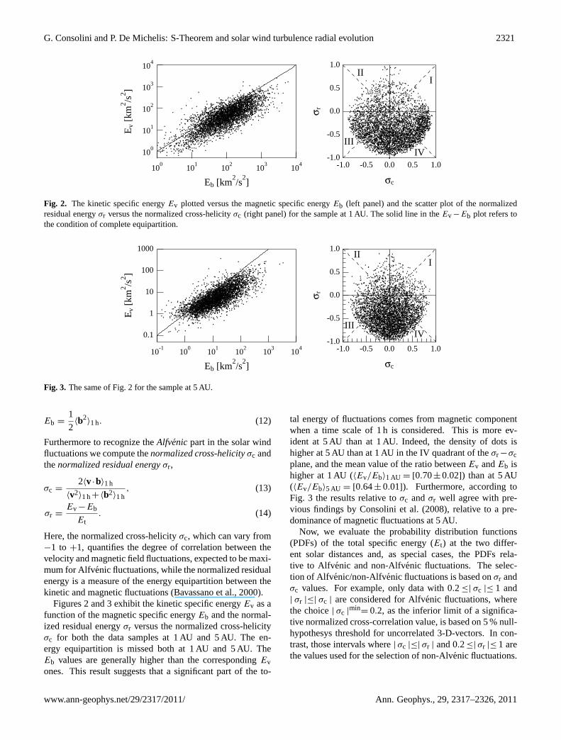
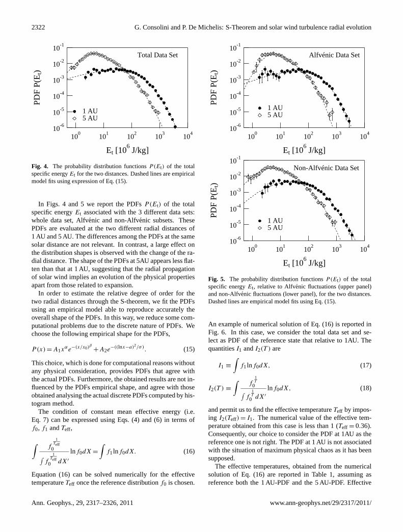
Fig. 4. The probability distribution functionsP(Et) of the totalspecific energyEt for the two distances. Dashed lines are empiricalmodel fits using expression of Eq. (15).

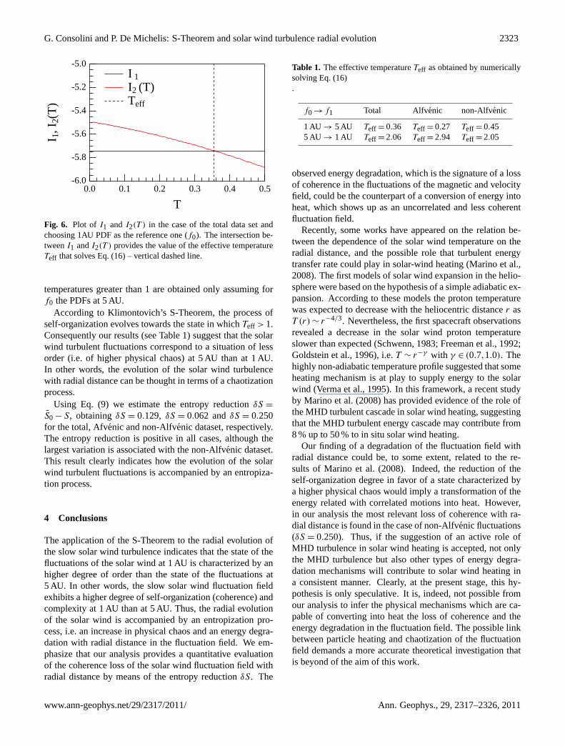
In Figs. 4 and 5 we report the PDFsP(Et) of the totalspecific energyEt associated with the 3 different data sets:whole data set, Alfvenic and non-Alfvenic subsets. ThesePDFs are evaluated at the two different radial distances of1 AU and 5 AU. The differences among the PDFs at the samesolar distance are not relevant. In contrast, a large effect onthe distribution shapes is observed with the change of the ra-dial distance. The shape of the PDFs at 5AU appears less flat-ten than that at 1 AU, suggesting that the radial propagationof solar wind implies an evolution of the physical propertiesapart from those related to expansion.

In order to estimate the relative degree of order for thetwo radial distances through the S-theorem, we fit the PDFsusing an empirical model able to reproduce accurately theoverall shape of the PDFs. In this way, we reduce some com-putational problems due to the discrete nature of PDFs. Wechoose the following empirical shape for the PDFs,

P(x) = A1xαe−(x/x0)

β

+A2e−((lnx−a)2/σ). (15)

This choice, which is done for computational reasons withoutany physical consideration, provides PDFs that agree withthe actual PDFs. Furthermore, the obtained results are not in-fluenced by the PDFs empirical shape, and agree with thoseobtained analysing the actual discrete PDFs computed by his-togram method.

The condition of constant mean effective energy (i.e.Eq. 7) can be expressed using Eqs. (4) and (6) in terms off0, f1 andTeff,

∫f

1Teff

0∫f

1Teff

0 dX′

lnf0dX =

∫f1lnf0dX. (16)

Equation (16) can be solved numerically for the effectivetemperatureTeff once the reference distributionf0 is chosen.

10-6

10-5

10-4

10-3

10-2

10-1

PDF

P(E

t)

100

101

102

103

104

Et [106 J/kg]

1 AU 5 AU

Alfvénic Data Set

10-6

10-5

10-4

10-3

10-2

10-1

PDF

P(E

t)

100

101

102

103

104

Et [106 J/kg]

1 AU 5 AU

Non-Alfvénic Data Set

Fig. 5. The probability distribution functionsP(Et) of the totalspecific energyEt, relative to Alfvenic fluctuations (upper panel)and non-Alfvenic fluctuations (lower panel), for the two distances.Dashed lines are empirical model fits using Eq. (15).

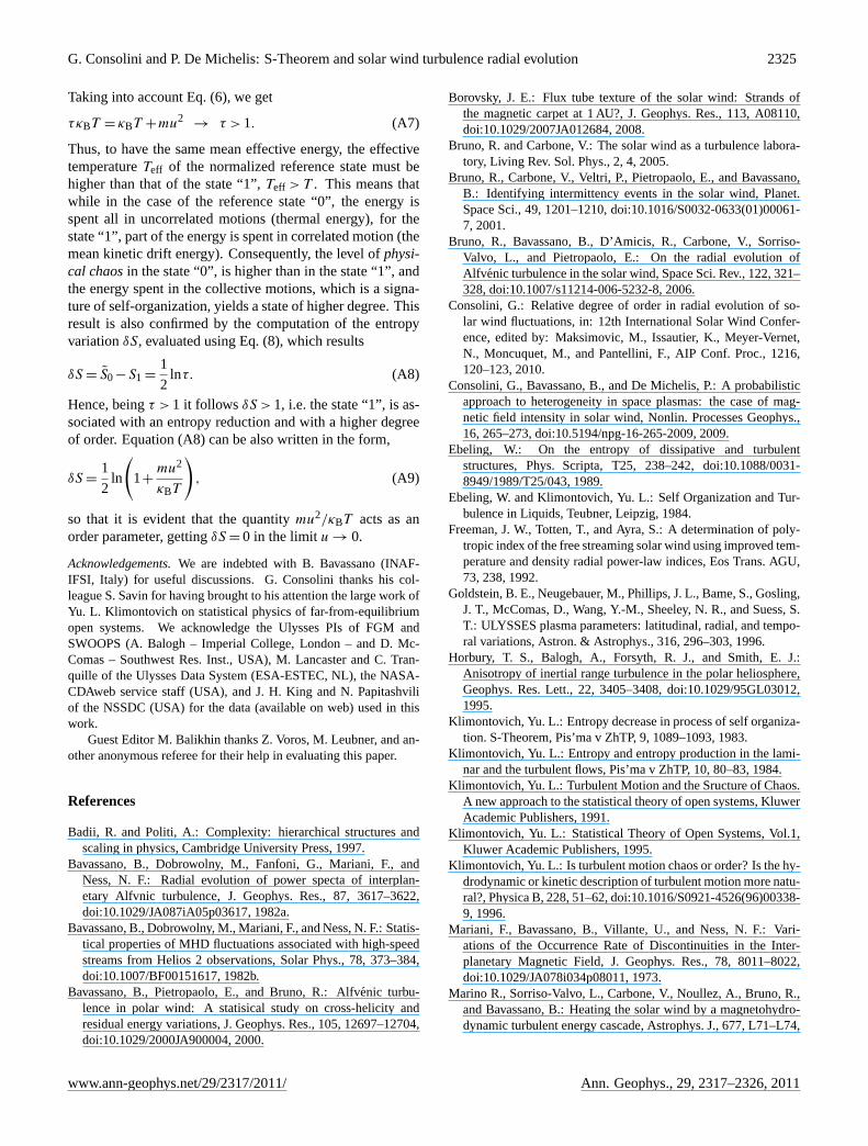
An example of numerical solution of Eq. (16) is reported inFig. 6. In this case, we consider the total data set and se-lect as PDF of the reference state that relative to 1AU. ThequantitiesI1 andI2(T ) are

I1 ≡

∫f1lnf0dX, (17)

I2(T ) ≡

∫f

1T

0∫f

1T

0 dX′

lnf0dX, (18)

and permit us to find the effective temperatureTeff by impos-ing I2(Teff) = I1. The numerical value of the effective tem-perature obtained from this case is less than 1 (Teff = 0.36).Consequently, our choice to consider the PDF at 1AU as thereference one is not right. The PDF at 1 AU is not associatedwith the situation of maximum physical chaos as it has beensupposed.

The effective temperatures, obtained from the numericalsolution of Eq. (16) are reported in Table1, assuming asreference both the 1 AU-PDF and the 5 AU-PDF. Effective

Ann. Geophys., 29, 2317–2326, 2011 www.ann-geophys.net/29/2317/2011/

G. Consolini and P. De Michelis: S-Theorem and solar wind turbulence radial evolution 2323

-6.0

-5.8

-5.6

-5.4

-5.2

-5.0I 1

, I2(

T)

0.50.40.30.20.10.0

T

I 1

I2 (T) Teff

Fig. 6. Plot of I1 and I2(T ) in the case of the total data set andchoosing 1AU PDF as the reference one (f0). The intersection be-tweenI1 andI2(T ) provides the value of the effective temperatureTeff that solves Eq. (16) – vertical dashed line.

temperatures greater than 1 are obtained only assuming forf0 the PDFs at 5 AU.

According to Klimontovich’s S-Theorem, the process ofself-organization evolves towards the state in whichTeff > 1.Consequently our results (see Table1) suggest that the solarwind turbulent fluctuations correspond to a situation of lessorder (i.e. of higher physical chaos) at 5 AU than at 1 AU.In other words, the evolution of the solar wind turbulencewith radial distance can be thought in terms of a chaotizationprocess.

Using Eq. (9) we estimate the entropy reductionδS =

S0 − S, obtainingδS = 0.129, δS = 0.062 andδS = 0.250for the total, Afvenic and non-Alfvenic dataset, respectively.The entropy reduction is positive in all cases, although thelargest variation is associated with the non-Alfvenic dataset.This result clearly indicates how the evolution of the solarwind turbulent fluctuations is accompanied by an entropiza-tion process.

4 Conclusions

The application of the S-Theorem to the radial evolution ofthe slow solar wind turbulence indicates that the state of thefluctuations of the solar wind at 1 AU is characterized by anhigher degree of order than the state of the fluctuations at5 AU. In other words, the slow solar wind fluctuation fieldexhibits a higher degree of self-organization (coherence) andcomplexity at 1 AU than at 5 AU. Thus, the radial evolutionof the solar wind is accompanied by an entropization pro-cess, i.e. an increase in physical chaos and an energy degra-dation with radial distance in the fluctuation field. We em-phasize that our analysis provides a quantitative evaluationof the coherence loss of the solar wind fluctuation field withradial distance by means of the entropy reductionδS. The

Table 1. The effective temperatureTeff as obtained by numericallysolving Eq. (16).

f0 → f1 Total Alfvenic non-Alfvenic

1 AU → 5 AU Teff = 0.36 Teff = 0.27 Teff = 0.455 AU → 1 AU Teff = 2.06 Teff = 2.94 Teff = 2.05

observed energy degradation, which is the signature of a lossof coherence in the fluctuations of the magnetic and velocityfield, could be the counterpart of a conversion of energy intoheat, which shows up as an uncorrelated and less coherentfluctuation field.

Recently, some works have appeared on the relation be-tween the dependence of the solar wind temperature on theradial distance, and the possible role that turbulent energytransfer rate could play in solar-wind heating (Marino et al.,2008). The first models of solar wind expansion in the helio-sphere were based on the hypothesis of a simple adiabatic ex-pansion. According to these models the proton temperaturewas expected to decrease with the heliocentric distancer asT (r) ∼ r−4/3. Nevertheless, the first spacecraft observationsrevealed a decrease in the solar wind proton temperatureslower than expected (Schwenn, 1983; Freeman et al., 1992;Goldstein et al., 1996), i.e.T ∼ r−γ with γ ∈ (0.7,1.0). Thehighly non-adiabatic temperature profile suggested that someheating mechanism is at play to supply energy to the solarwind (Verma et al., 1995). In this framework, a recent studyby Marino et al.(2008) has provided evidence of the role ofthe MHD turbulent cascade in solar wind heating, suggestingthat the MHD turbulent energy cascade may contribute from8 % up to 50 % to in situ solar wind heating.

Our finding of a degradation of the fluctuation field withradial distance could be, to some extent, related to the re-sults of Marino et al.(2008). Indeed, the reduction of theself-organization degree in favor of a state characterized bya higher physical chaos would imply a transformation of theenergy related with correlated motions into heat. However,in our analysis the most relevant loss of coherence with ra-dial distance is found in the case of non-Alfvenic fluctuations(δS = 0.250). Thus, if the suggestion of an active role ofMHD turbulence in solar wind heating is accepted, not onlythe MHD turbulence but also other types of energy degra-dation mechanisms will contribute to solar wind heating ina consistent manner. Clearly, at the present stage, this hy-pothesis is only speculative. It is, indeed, not possible fromour analysis to infer the physical mechanisms which are ca-pable of converting into heat the loss of coherence and theenergy degradation in the fluctuation field. The possible linkbetween particle heating and chaotization of the fluctuationfield demands a more accurate theoretical investigation thatis beyond of the aim of this work.

www.ann-geophys.net/29/2317/2011/ Ann. Geophys., 29, 2317–2326, 2011

2324 G. Consolini and P. De Michelis: S-Theorem and solar wind turbulence radial evolution

In connection with the evolution of the turbulenceanisotropy character, the observed loss of coherence couldsuggest that, in agreement with the results ofHorbury et al.(1995) for the polar wind, the radial evolution is accompa-nied by an increase in isotropy at larger heliospheric dis-tances also in the case of slow equatorial solar wind. More-over, the overall decrease in the degree of order with radialdistance suggests that we could be in the presence of a pro-cess of decaying turbulence in the case of slow solar wind.This hypothesis is supported by the following arguments.

The S-Theorem application to hydrodynamic turbulentflows (Prigogine and Stengers, 1984; Ebeling and Klimon-tovich, 1984; Klimontovich, 1984; Ebeling, 1989) demon-strates that, in contrast to the almost universally acceptedview, turbulent flows at high Reynolds numbers are more or-dered than laminar ones at low Reynolds numbers. This canbe explained considering that in the first case a large percent-age of energy is concentrated in the collective modes of hy-drodynamic motions (Ebeling, 1989; Klimontovich, 1996).This point is confirmed by the S-Theorem that, when ap-plied to the transition from laminar to turbulent flow, exhibitsa positive value of the entropy difference between the twostates. Indeed, as it is clearly shown byKlimontovich(1996),we have:

T [Slam−Sturb] =mn

2〈(δu)2

〉 > 0. (19)

where〈(δu)2〉 depends the sum of the diagonal elements in

the Reynolds stress tensor. Thus, steady turbulent motionsare more ordered than laminar ones, i.e. the transition to tur-bulence is an example of self-organization process emergingfrom a collective dynamics. However, the emergence of self-organization in turbulence flows can also be understood interms of an increase in coherence in macroscopic motions ac-companied by a decrease in the degree of spatial symmetries.

In the previous work on magnetic field intensity fluctu-ations byConsolini (2010) it was observed an increase inthe degree of order with radial distance. This result wasread in terms of an increasing relevance of magnetic coher-ent structures with radial distance. As noted inBruno et al.(2006) there could be two different mechanisms responsi-ble for the increasing relevance of coherent magnetic struc-tures: (i) these could be a byproduct of Alfvenic turbulenceor (ii) the remnants of structures produced at the Sun. Al-thoughConsolini (2010) suggested that coherent structuresmay be generated from turbulence evolution with radial dis-tance, the hypothesis that coherent magnetic structures areremnants of structures produced at the solar surface cannotbe excluded in light of our results on the decrease of the rel-ative order in the turbulent fluctuation field. Indeed, the de-caying/degradation of the solar wind turbulence with radialdistance, which is accompanied by a decrease in the turbulentfluctuation amplitude, could imply the emergence of the un-derlining solar wind structures originated at the Sun. Clearly,

at the present stage this aspect is still only speculative and de-serves a more accurate analysis.

In conclusion, we clearly show that the evolution of slowsolar wind turbulence with radial distance is accompaniedby a degradation process. More work is necessary to extendthese results to different solar wind conditions, although theextension to fast streams is not straightforward.

Appendix A

On the meaning of the effective temperatureT eff

To clarify the meaning of the effective temperatureTeff as ameasure of the degree of order, a simple illustrative exam-ple, that can also be found inKlimontovich (1991), is hereextensively discussed

Let it be f0(v) andf1(v) the velocity distribution func-tions for two 1-D systems consisting of particles of massm

and at the same temperatureT , i.e.

f0(v) =

√m

2πκBTexp

(−

mv2

2κBT

), (A1)

f1(v) =

√m

2πκBTexp

(−

m(v−u)2

2κBT

), (A2)

where the velocityu is relative to a coherent bulk motion.Consider the distribution functionf0 as the reference one.According to Eq. (3), we introduce the effective HamiltonianHeff,

Heff = −lnf0 'mv2

2κBT, (A3)

where the last equality is valid unless of a constant factor.From this expression we evaluate the mean effective energyfor the two states;

〈Heff〉0 =1

2, (A4)

〈Heff〉1 =κBT +mu2

2κBT. (A5)

These two states do not have the same mean effective energy,being〈Heff〉1 > 〈Heff〉0, and, consequently it is not possibleto evaluate directly the relative entropyδS.

According to the Klimontovich’s S-Theorem procedure,we can renormalize the distribution of the reference state,represented byf0, so that the renormalized distributionf0acquires the same mean effective energy of the state “1”. Todo this, following the renormalization procedure, we intro-duce an effective temperatureTeff (see Eqs.3and5) and writethe new renormalized distributionf0 in the form,

f0(v) =

√m

2πκBTeffexp

(−

mv2

2κBTeff

), Teff = τT . (A6)

Ann. Geophys., 29, 2317–2326, 2011 www.ann-geophys.net/29/2317/2011/

G. Consolini and P. De Michelis: S-Theorem and solar wind turbulence radial evolution 2325

Taking into account Eq. (6), we get

τκBT = κBT +mu2→ τ > 1. (A7)

Thus, to have the same mean effective energy, the effectivetemperatureTeff of the normalized reference state must behigher than that of the state “1”,Teff > T . This means thatwhile in the case of the reference state “0”, the energy isspent all in uncorrelated motions (thermal energy), for thestate “1”, part of the energy is spent in correlated motion (themean kinetic drift energy). Consequently, the level ofphysi-cal chaosin the state “0”, is higher than in the state “1”, andthe energy spent in the collective motions, which is a signa-ture of self-organization, yields a state of higher degree. Thisresult is also confirmed by the computation of the entropyvariationδS, evaluated using Eq. (8), which results

δS = S0−S1 =1

2lnτ. (A8)

Hence, beingτ > 1 it follows δS > 1, i.e. the state “1”, is as-sociated with an entropy reduction and with a higher degreeof order. Equation (A8) can be also written in the form,

δS =1

2ln

(1+

mu2

κBT

), (A9)

so that it is evident that the quantitymu2/κBT acts as anorder parameter, gettingδS = 0 in the limitu → 0.

Acknowledgements.We are indebted with B. Bavassano (INAF-IFSI, Italy) for useful discussions. G. Consolini thanks his col-league S. Savin for having brought to his attention the large work ofYu. L. Klimontovich on statistical physics of far-from-equilibriumopen systems. We acknowledge the Ulysses PIs of FGM andSWOOPS (A. Balogh – Imperial College, London – and D. Mc-Comas – Southwest Res. Inst., USA), M. Lancaster and C. Tran-quille of the Ulysses Data System (ESA-ESTEC, NL), the NASA-CDAweb service staff (USA), and J. H. King and N. Papitashviliof the NSSDC (USA) for the data (available on web) used in thiswork.

Guest Editor M. Balikhin thanks Z. Voros, M. Leubner, and an-other anonymous referee for their help in evaluating this paper.

References

Badii, R. and Politi, A.: Complexity: hierarchical structures andscaling in physics, Cambridge University Press, 1997.

Bavassano, B., Dobrowolny, M., Fanfoni, G., Mariani, F., andNess, N. F.: Radial evolution of power specta of interplan-etary Alfvnic turbulence, J. Geophys. Res., 87, 3617–3622,doi:10.1029/JA087iA05p03617, 1982a.

Bavassano, B., Dobrowolny, M., Mariani, F., and Ness, N. F.: Statis-tical properties of MHD fluctuations associated with high-speedstreams from Helios 2 observations, Solar Phys., 78, 373–384,doi:10.1007/BF00151617, 1982b.

Bavassano, B., Pietropaolo, E., and Bruno, R.: Alfvenic turbu-lence in polar wind: A statisical study on cross-helicity andresidual energy variations, J. Geophys. Res., 105, 12697–12704,doi:10.1029/2000JA900004, 2000.

Borovsky, J. E.: Flux tube texture of the solar wind: Strands ofthe magnetic carpet at 1 AU?, J. Geophys. Res., 113, A08110,doi:10.1029/2007JA012684, 2008.

Bruno, R. and Carbone, V.: The solar wind as a turbulence labora-tory, Living Rev. Sol. Phys., 2, 4, 2005.

Bruno, R., Carbone, V., Veltri, P., Pietropaolo, E., and Bavassano,B.: Identifying intermittency events in the solar wind, Planet.Space Sci., 49, 1201–1210,doi:10.1016/S0032-0633(01)00061-7, 2001.

Bruno, R., Bavassano, B., D’Amicis, R., Carbone, V., Sorriso-Valvo, L., and Pietropaolo, E.: On the radial evolution ofAlfv enic turbulence in the solar wind, Space Sci. Rev., 122, 321–328,doi:10.1007/s11214-006-5232-8, 2006.

Consolini, G.: Relative degree of order in radial evolution of so-lar wind fluctuations, in: 12th International Solar Wind Confer-ence, edited by: Maksimovic, M., Issautier, K., Meyer-Vernet,N., Moncuquet, M., and Pantellini, F., AIP Conf. Proc., 1216,120–123, 2010.

Consolini, G., Bavassano, B., and De Michelis, P.: A probabilisticapproach to heterogeneity in space plasmas: the case of mag-netic field intensity in solar wind, Nonlin. Processes Geophys.,16, 265–273,doi:10.5194/npg-16-265-2009, 2009.

Ebeling, W.: On the entropy of dissipative and turbulentstructures, Phys. Scripta, T25, 238–242,doi:10.1088/0031-8949/1989/T25/043, 1989.

Ebeling, W. and Klimontovich, Yu. L.: Self Organization and Tur-bulence in Liquids, Teubner, Leipzig, 1984.

Freeman, J. W., Totten, T., and Ayra, S.: A determination of poly-tropic index of the free streaming solar wind using improved tem-perature and density radial power-law indices, Eos Trans. AGU,73, 238, 1992.

Goldstein, B. E., Neugebauer, M., Phillips, J. L., Bame, S., Gosling,J. T., McComas, D., Wang, Y.-M., Sheeley, N. R., and Suess, S.T.: ULYSSES plasma parameters: latitudinal, radial, and tempo-ral variations, Astron. & Astrophys., 316, 296–303, 1996.

Horbury, T. S., Balogh, A., Forsyth, R. J., and Smith, E. J.:Anisotropy of inertial range turbulence in the polar heliosphere,Geophys. Res. Lett., 22, 3405–3408,doi:10.1029/95GL03012,1995.

Klimontovich, Yu. L.: Entropy decrease in process of self organiza-tion. S-Theorem, Pis’ma v ZhTP, 9, 1089–1093, 1983.

Klimontovich, Yu. L.: Entropy and entropy production in the lami-nar and the turbulent flows, Pis’ma v ZhTP, 10, 80–83, 1984.

Klimontovich, Yu. L.: Turbulent Motion and the Sructure of Chaos.A new approach to the statistical theory of open systems, KluwerAcademic Publishers, 1991.

Klimontovich, Yu. L.: Statistical Theory of Open Systems, Vol.1,Kluwer Academic Publishers, 1995.

Klimontovich, Yu. L.: Is turbulent motion chaos or order? Is the hy-drodynamic or kinetic description of turbulent motion more natu-ral?, Physica B, 228, 51–62,doi:10.1016/S0921-4526(96)00338-9, 1996.

Mariani, F., Bavassano, B., Villante, U., and Ness, N. F.: Vari-ations of the Occurrence Rate of Discontinuities in the Inter-planetary Magnetic Field, J. Geophys. Res., 78, 8011–8022,doi:10.1029/JA078i034p08011, 1973.

Marino R., Sorriso-Valvo, L., Carbone, V., Noullez, A., Bruno, R.,and Bavassano, B.: Heating the solar wind by a magnetohydro-dynamic turbulent energy cascade, Astrophys. J., 677, L71–L74,

www.ann-geophys.net/29/2317/2011/ Ann. Geophys., 29, 2317–2326, 2011

2326 G. Consolini and P. De Michelis: S-Theorem and solar wind turbulence radial evolution

doi:10.1086/587957, 2008.McCracken, K. G. and Ness, N. F.: The Collimation of Cosmic

Rays by the Interplanetary Magnetic Field, J. Geophys. Res., 71,3315–3318,doi:10.1029/JZ071i013p03315, 1966.

Ness, N. F., Scearce, C. S., and Cantarano, S.: Preliminary Resultsfrom the Pioneer 6 Magnetic Field Experiment, J. Geophys. Res.,71, 3305–3313,doi:10.1029/JZ071i013p03305, 1966.

Nicolis, G. and Nicolis, C.: Foundations of Complex Systems. Non-linear Dynamics, Statistical Physics, Information and Prediction,World Scientific Publishing Co. Pte. Ltd., 2007.

Prigogine, I. and Stengers, I.: Order out of chaos, Heinemamm,London, 1984.

Roberts, D. A., Goldstein, M. L., Klein, L. W., and Matthaeus, W.H.: Origin and evolution of fluctuations in the solar wind: Heliosobservations and Helios-Voyager comparisons, J. Geophys. Res.,92, 12023–12035,doi:10.1029/JA092iA11p12023, 1987.

Russell, C. T.: Solar wind and interplanetary magnetic field: A tu-torial, Space Weather, Geophysical Monograph, 125, 2001.

Schwenn, R.: The average solar wind in the inner heliosphere:Structure and slow variations, in: Solar Wind FIVE, NASA Conf.Publ., CP-2280, 485, 1983.

Tu, C.-Y. and Marsch, E.: Evidence for a Background Spectrumof Solar Wind Turbulence in the Inner Heliosphere, J. Geophys.Res., 95, 4337–4341,doi:10.1029/JA095iA04p04337, 1990.

Tu C.-Y. and Marsch, E.: A Model of Solar Wind Fluctuations withTwo Components: Alfven Waves and Convective Structures, J.Geophys. Res., 98, 1257–1276,doi:10.1029/92JA01947, 1993.

Tu, C.-Y., Pu, Z.-Y., and Wei, F.-S.: The power spectrum of in-terplanetary Alfvenic fluctuations: deviation of the governingequation and its solution, J. Geophys. Res., 89, 9695–9702,doi:10.1029/JA089iA11p09695, 1984.

Tu, C.-Y., Marsch, E., and Thieme, K. M.: Basic properties ofsolar wind MHD turbulence near 0.3 AU analysed by meanof Elsasser variables, J. Geophys. Res., 94, 11739–11759,doi:10.1029/JA094iA09p11739, 1989.

Verma, M. K., Roberts, D. A., and Goldstein, M. L.: Turbulent heat-ing and temperature evolution in the solar wind plasma, J. Geo-phys. Res., 100, 19839–19850,doi:10.1029/95JA01216, 1995.

Ann. Geophys., 29, 2317–2326, 2011 www.ann-geophys.net/29/2317/2011/