Acausal Modelling and Dynamic Simulation of the Standalone Wind-Solar Plantusing Modelica

Arash M. Dizqah, Alireza Maheri, Krishna BusawonFaculty of Engineering and Environment

Northumbria UniversityNewcastle Upon Tyne, UK

arash.moradinegade@northumbria.ac.uk

Peter FritzsonDepartment of Computer Science

Linkoping UniversityLinkoping, Sweden

Abstract—In order to design model-based controllers appli-cable to hybrid renewable energy systems (HRES), it is essentialto model the HRES mathematically. In this study, a standaloneHRES, consisting of a photovoltaic (PV) array, a lead-acidbattery bank, a pitch-controlled wind turbine, and a three-phasepermanent magnet synchronous generator (PMSG), supplies avariable DC load demand through two boost- and buck-typeDC-DC converters. It is shown that the mathematical modelof the HRES can be represented by a system of nonlinearhybrid differential algebraic equations (hybrid DAEs). Thedeveloped model in this paper employs the Modelica languagethat allows object-oriented and acausal modelling of the multi-mode systems. The OpenModelica environment is utilised tocompile the model and simulate the system. It is shown thatthe simulation provides a sufficiently accurate prediction of allthe differential and algebraic states including mode transitions.The results of the simulation show a good match with theinformation available in the components datasheet.

Index Terms—photovoltaic (PV); battery; wind turbine; hy-brid renewable energy system (HRES), acausal modelling;hybrid DAE; Modelica.

I. INTRODUCTION

Advances in renewable energy technologies have increasedthe share of the sustainable energy in the growing electricitymarket. A conventional HRES consists of solar and wind gen-erators supplying DC, AC, or mixed electrical load demands.The system also consists of a battery bank to overcome thepower fluctuation introduced by uncertainty in the energyresources. Figure 1 illustrates the HRES topology in thisstudy that, without loss of generality, supplies a DC load.

The solar branch consists of a PV array connected to aDC-DC converter that boosts up the generated DC voltage tomatch the load characteristics [1]. Meanwhile, the variablespeed wind branch topology, consisting of a wind turbine,three-phase generator and rectifier, supplies the electrical en-ergy to the DC load through a buck-type converter. The DC-DC converters may be equipped with the maximum powerpoint tracker (MPPT) algorithms to harvest the maximumavailable power (e.g. see [2; 3]). While the solar irradiance,wind speed, and the load demand are the non-manipulatedvariables of the system, the operation of the HRES can becontrolled by three manipulated variables, namely, the pitchangle β of the wind turbine, the duty cycles of the wind- and

Fig. 1. The HRES topology in this study.

solar-branch, i.e. Dw and Ds ,respectively.In order to study the behavior of the HRES as well as to

design model-based controllers, it is essential to model andsimulate the system accurately. However, there are two majorchallenges, i.e. the algebraic constraints introduced by the PVmodule, wind turbine, and the battery, as well as the multi-mode operation of the battery. HRES introduces algebraic aswell as discrete states (causing discontinuity) [1; 4] leadingthe system to be modeled with hybrid DAEs [5] and hencerequires being simulated employing an acausal approach.

The causal approach, decomposes a system into a chainof causal interacting blocks, requires the system being onlycomposed of ordinary differential equations (ODE). On theother hand, the acausal modelling is a declarative approach,described with a modelling language such as Modelica [6],in which individual parts of the model are directly describedas HDAE equations [5]. Modelica, as an object-oriented andequation-based language to describe complex systems usingan acausal approach, provides the capability to model thehybrid systems [5]. Among a number of available implemen-tations of Modelica compiler, the open-source OpenModelicaenvironment [7], which provides a Modelica compiler andintegrated DAE solvers, supports more features of the Mod-elica language comparing with the others.

In this paper, a mathematical model of the HRES, which isapplicable to develop model-based strategies, is proposed as

2013 UKSim 15th International Conference on Computer Modelling and Simulation

978-0-7695-4994-1/13 $26.00 © 2013 IEEE

DOI 10.1109/UKSim.2013.145

580

HDAEs (Section II) [8]. Modelica is employed to developan acausal model of the system that is solved using ageneral purpose DAE solver (Section III). The results of thesimulation have been compared with information availablein the PV, battery, and wind turbine datasheets provided bythe manufacturers that indicate good accuracy (Section IV).

II. HRES MATHEMATICAL MODEL

Applying the model-based control strategies requires sim-ple and still accurate mathematical modelling of the HRES.Due to existence of simultaneous fast and slow dynamicswithin the HRES, its simulation is becoming time-consumingand memory expensive. However, the model-based con-trollers are normally the outer low speed (of the order ofseveral seconds) strategies, hence the fast dynamics can bereplaced with the relevant steady-state equations.

A. The solar branch

The authors in [1] presented a mathematical model of thesolar branch consisting of a PV array, boost-type DC-DCconverter, and a lead-acid battery bank. The presented modelin [1] is based on the equivalent circuits of the PV module[9; 10] and the battery [11] as well as the average modelof the converter [12]. However, the average model of theconverter can be replaced with the steady-state equations (1)in the continuous conduction mode (CCM) [12] as follows:

Vbstack =Vpv

1 −Ds(1a)

Ipvdc = Ipv × (1 −Ds) (1b)

where Ds is the switching duty cycle of the converter.Fig. 2 illustrates a single-diode equivalent circuit of a

PV module. The performance of different PV modules aremeasured at the standard test condition (STC) [10]. Applyingthe Kirchhoff current law (KCL) to the junction point of theseries and shunt resistors gives the characteristic equation(2a) of the PV module. The photocurrent Iph and the diodereverse saturation current I0 are calculated with (2b) and (2c)[10].

Ipv = Iph − I0

exp(

Vpv +RsIpvndNs

q

KTc) − 1

−

Vpv +RsIpvRsh

, (2a)

Iph =

(Rs +RshRsh

Isc,stc + kI (Tc − Tc,stc)

)S

Sstc, (2b)

I0 =Isc,stc + kI (Tc − Tc,stc)

exp(Voc,stc + kV (Tc − Tc,stc)

ndNs

q

KTc) − 1

. (2c)

where the experimental parameters indicated in Fig. 2 requirebeing identified for each type of the PV module, and allothers are as follows:

Fig. 2. The single-diode equivalent electrical circuit of a PV module.

q The electron charge (1.6021810−19)K The Boltzman constant (1.3806610−23)Ns The number of the PV cells in series as the PV module (-)Tc The current amount of the PV cell temperature (K)Isc,stc The short-circuit current of the PV module at the STC (A)kI The temperature coefficient of the short-circuit current (A/C)kV The temperature coefficient of the open-circuit voltage (V/C)S The current amount of the solar irradiance (W/m)Sstc The amount of the solar irradiance at the STC (W/m)Tc,stc The amount of the cell temperature at the STC (K)Voc,stc The open-circuit voltage of the PV module at the STC (V)

The authors in [11] introduced a model of the lead-acidbattery as the following hybrid DAEs which present twomodes of operation, namely, charging and discharging:

Vbstack = Nb ×

V0 −RIbat + Vexp−P1Cmax

Cmax −QactQact−

P1Cmax

Qact + 0.1CmaxIf charging,

V0 −RIbat + Vexp+

P1Cmax

Qact − CmaxQact+

P1Cmax

Qact − CmaxIf discharging,

(3a)

Modebat =

charging If ≤ 0,

discharging If > 0,(3b)

SOC = 1−Qact

Cmax, (3c)

dQact

dt(t) =

1

3600Ibat(t), (3d)

dVexp

dt(t) =

P2

3600|Ibat|(P3 − Vexp) charging,

−P2

3600|Ibat|Vexp discharging,

(3e)

dIf

dt(t) = −

1

Ts(If − Ibat). (3f)

where Vbstack, Ibat and SOC, respectively, are the voltage,current, and the state of charge of the Nb batteries in series,constructing a battery stack. The parameters P1-P3 are theexperimental parameters require being identified for eachtype of the battery and Vexp smooths the battery voltageduring the mode transition period. The Cmax is the maximumamount of the battery capacity, R is the internal resistor ofthe battery, Qact is the actual battery capacity, and V0 is the

581

Fig. 3. The power coefficient curve, with respect to the tip speed ratio, forthree different values of the pitch angle.

battery constant voltage. If is also a filtered value of thebattery current with the time constant of Ts [11].

B. Wind branch

1) Wind turbine (WT): Having the nominal power ofthe WT, Pnom, the generated mechanical power (4a) iscalculated based on the per unit (p.u.) power coefficientCp,p.u.. The performance of a WT can be characterized withan experimental power coefficient curve [3]. Fig. 3 illustratesthe power coefficient for different tip speed ratio λ, whichis the weighted ratio of the angular velocity of the generatorrotor ωr to the wind speed Ux (4b). The maximum power co-efficient Cp,max locates at the optimum tip speed ratio valueλopt and is limited to 0.593, according to the Lanchaster-Betz theory [3]. In this study, the experimental Cp curve ismodeled by (4d) [13], chiefly because MATLAB/SIMULINKhas also adopted this model. This wind turbine, with the bladeradius Rad of 4.01 meter, generates the maximum powercoefficient Cp,max of around 0.48 at the optimum tip speedratio of 8.1.

Pm = Cp,p.u.(Ux

Ux,base)3Pnom, (4a)

λ =Rad× ωr

Ux, (4b)

λi = (1

λ+ 0.08β−

0.035

β3 + 1)−1, (4c)

Cp,p.u. =1

Cp,max(C1(

C2

λi− C3β − C4)exp(−

C5

λi) + C6λ). (4d)

The experimental coefficients C1−C6 are defined in TABLEII and β is the blades pitch angle [3]. λi is the intermediatevariable to make the equations easier to understand.

2) Permanent magnet synchronous generator (PMSG): Inspite of high cost, the PMSG is the most dominant type ofthe direct-drive generators in the market [14], chiefly due tohigher efficiency. In order to make the mathematical model ofthe PMSG suitable for the model-based controllers, exceptthe angular velocity (5a) all other fast voltage and currentdynamics are ignored. Moreover, it is assumed that there isno mechanical and electrical loss through the powertrain, forsimplicity’s sake. As a result, the electromagnetic power, as

Fig. 4. The electrical circuit of the full-bridge three-phase rectifier.

the product of the electromagnetic torque Te and the angularvelocity ωr, is equal to the output electrical power of thewind branch (5b) (Fig. 1).

In order to apply the PMSG to the direct-drive topology(5c), it requires increasing the number of the pole pairs P[14]. The electrical frequency ωe, as a result, is P times fasterthan the mechanical angular velocity ωr (5d).

dωr

dt(t) =

1

J(Te − Tm − Fωr), (5a)

− Te × ωr = IWTDC × Vbstack, (5b)

− Tm × ωr = (Cp,p.u.(Ux

Ux,base)3Pnom, (5c)

ωe = Pωr, (5d)

VLL =1√2kEωr, (5e)

kE =√3Pψ. (5f)

The shaft inertia J (Kg.m2) and the combined viscousfriction coefficient F (N.m.s) of the PMSG are given bythe manufacturers. The VLL, i.e. the r.m.s. value of theline-to-line output voltage of the generator, depends on themechanical angular velocity (5e). Having the number of thepole pairs P and the flux linkage ψ (V.s) of the generator(TABLE II), the voltage constant kE is calculated (5f).

3) 3-Phase rectifier: Fig. 4 illustrates the electrical circuitof a full-bridge three-phase rectifier where Iwt is the equiva-lent DC current of the dc side. Due to the inductance Ls onthe ac side, there is non-instantaneous current commutation[12]. The average output DC voltage Vwt in presence ofthe non-instantaneous current commutation is calculated asfollows:

Vwt = 1.35VLL −3

πωeLsIwt, (6)

4) Buck-type DC-DC converter: The hybrid or averagemodels of the buck-type DC-DC converter can be replacedwith the relevant steady-state CCM equations (7) [12], whichis applicable to model-based outer controllers.

Vbstack = VwtDw, (7a)

Iwt = IwtdcDw. (7b)

582

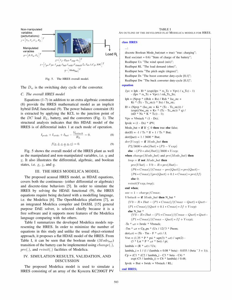
Fig. 5. The HRES overall model.

The Dw is the switching duty cycle of the converter.

C. The overall HRES model

Equations (1-7) in addition to an extra algebraic constraint(8) provide the HRES mathematical model as an implicithybrid DAE functional (9). The power balance constraint (8)is extracted by applying the KCL to the junction point ofthe DC load RL, battery, and the converters (Fig. 1). Thestructural analysis indicates that this HDAE model of theHRES is of differential index 1 at each mode of operation.

Ipvdc + Iwtdc + Ibat −Vbstack

RL= 0. (8)

f(x, x, z, q, u, v) = 0. (9)

Fig. 5 shows the overall model of the HRES plant as wellas the manipulated and non-manipulated variables, i.e. u andv. It also illustrates the differential, algebraic, and booleanstates, i.e. x, z, and q.

III. THE HRES MODELICA MODELThe proposed acausal HRES model, as HDAE equations,

covers both the continuous- (either differential or algebraic)and discrete-time behaviors [5]. In order to simulate theHRES by solving the HDAE functional (9), the HRESequations require being declared with a modelling language,i.e. the Modelica [6]. The OpenModelica platform [7], asan integrated Modelica compiler and DASSL [15] generalpurpose DAE solver, is selected chiefly because it is afree software and it supports more features of the Modelicalanguage comparing with the others.

Table I summarizes the developed Modelica models rep-resenting the HRES. In order to minimize the number ofequations in this study and unlike the usual object-orientedapproach, it proposes a flat HDAE model of the HRES. FromTable I, it can be seen that the boolean mode (Modebat)transition of the battery can be implemented using change(.),pre(.), and reinit(.) facilities of Modelica.

IV. SIMULATION RESULTS, VALIDATION, ANDDISCUSSION

The proposed Modelica model is used to simulate aHRES consisting of an array of the Kyocera KC200GT PV

TABLE IAN OUTLINE OF THE DEVELOPED FLAT MODELICA MODELS FOR HRES.

class HRES

...;

discrete Boolean Mode bat(start = true) ”true: charging”;

Real soc(start = 0.6) ”State of charge of the battery”;

RealInput Ux ”The wind speed (m/s)”;

RealInput RL ”The load demand (ohm)”;

RealInput beta ”The pitch angle (degree)”;

RealInput Ds ”The boost converter duty-cycle [0,1]”;

RealInput Dw ”The buck converter duty-cycle [0,1]”;

equation

Ipv = Iph - I0 * (exp((Ipv * rs Tc + Vpv) / a Tc) - 1)- (Ipv * rs Tc + Vpv) / rsh Tc Sx;

Iph = (Npvp * ((Rsh + Rs) / Rsh * Isc stc +Ki * (Tc - Tc stc)) * Sx) / Sx stc;

I0 = (Npvp * (Isc stc + Ki * (Tc - Tc stc))) /(exp(((Voc stc + Kv * (Tc - Tc stc)) * q) /(nD * Ns * K * Tc)) - 1);

Vpv = Vbstack * (1 - Ds);

Ipvdc = (1 - Ds) * iPV;

Mode bat = if If ≤ 0 then true else false;

der(If) = -1 / Ts * If + 1 / Ts * Ibat;

der(Qact) = 1 / 3600 * Ibat;

der(V exp) = if Mode bat thenP2/3600 ∗ abs(Ibat) ∗ (P3− V exp)else −(P2 ∗ abs(Ibat))/3600 ∗ V exp;

when change(Mode bat) and pre(Mode bat) thentmp = if not Mode bat thenpre(V bat)− V 0−R ∗ pre(Ibat)−(P6 ∗ Cmax)/(Cmax− pre(Qact)) ∗ pre(Qact)−(P6 ∗ Cmax)/(pre(Qact) + 0.1 ∗ Cmax) ∗ pre(If)else 0;

reinit(V exp, tmp);

end when;

soc = 1− charge/Cmax;

V bstack = if Mode bat then N bat *

(V 0−R ∗ Ibat− (P1 ∗ Cmax)/(Cmax−Qact) ∗Qact−(P1 ∗ Cmax)/(Qact+ 0.1 ∗ Cmax) ∗ If + V exp)

else N bat *(V 0−R ∗ Ibat− (P1 ∗Cmax)/(Cmax−Qact) ∗Qact−(P1 ∗ Cmax)/(Cmax−Qact) ∗ If + V exp);

-Te * ωr = Iwtdc * Vbstack;

-Tm * ωr = Cp pu * (Ux / 12)ˆ3 * Pnom;

der(ωr) = (Te - Tm - F * ωr) / J;

Vwt = (1.35 * P * psi * sqrt(3) * ωr) / sqrt(2) -(3 * Lst * P * ωr * Iwt) / pi;

lambda = (R * ωr) / Ux;

lambda i = 1 / (1 / (lambda + 0.08 * beta) - 0.035 / (beta ˆ 3 + 1));

Cp = (C1 * (C2 / lambda i - C3 * beta - C4) *exp(-C5 / lambda i) + C6 * lambda) / 0.48;

Ipvdc + Ibat + Iwtdc = Vbstack / RL;

end HRES;

583

TABLE IIDIFFERENT PARAMETERS IN THIS STUDY (DIMENSIONS AS GIVEN IN

THE TEXT).

Wind turbine PMSG Battery stack PV moduleC1 0.517 J 35 Cmax 12.02 Rs 0.221C2 116 F 0.2 R 0.021 Rsh 405.4C3 0.4 P 8 V0 12.37 nd 1.3C4 5 ψ 0.8 P1 0.9 Ns 54C5 21 Pr 10K P2 20.73 Isc,stc 8.21C6 0.007 Ls 0.01 P3 0.55 Voc,stc 32.9λopt 8.1 − - Ts 0.726 kI 0.003Pnom 10K − - Nb 4 kV -0.12Rad 4.01 − - − - − -Ux,base 12 − - − - − -Cp,max 0.48 − - − - − -

modules and a bank of the Panasonic LC-R127R2PG lead-acid batteries. The authors in [10] and [11], respectively,presented the identified electrical parameters of the employedPV module and the lead-acid battery. TABLE II summarizesall parameters and their values in this study.

Fig. 6 compares the simulated current-voltage (I − V )curve of the KC200GT PV module at the STC conditionwith the experimental curve available by the manufacturer indatasheet (the circle markers). It is observed that the proposedmodel predicts the curve very close to the empirical dataprovided by the manufacturer.

Also, Fig. 7 illustrates the simulation results of a singleLC-R127R2PG lead-acid battery for a full operating cycleincluding charging, over-charging, saturation, discharging,over-discharging, and exhaustion zones. While the battery isbeing charged for 100 minutes, it is discharged afterward.It also indicates that after 25 minutes it enters into theover-charging zone. Discharging with the current of 7.2Ain average, it takes around 35 minutes for the battery, whichmatches with the information available in datasheet, to reachthe cut-off voltage that is around 10.2V .

The stability of the developed model is examined bysimulating the following sample scenario that applies dif-ferent step changes to the manipulated and non-manipulatedvariables:

• Simulation period is 700 seconds.• The solar irradiance is 1000W/m2 and the cell temper-

ature is 25C.• The PV array consists of 10 connected KC200GT PV

modules in parallel arrangement.• The battery bank consists of 20 battery stacks in par-

allel. Each battery stack consists of 4 connected LC-R127R2PG lead-acid batteries in series arrangement.

• After 100 seconds there is a step change in load resistorfrom 0.3 to 1.1Ω.

• There is a step change in wind speed at time 300 secondsfrom 12 to 20(m/s).

• A step change in the buck converter duty cycle at time500 seconds makes the wind turbine to be fully stalled.

Fig. 8 illustrates the manipulated variables applied by thecontroller to harvest the maximum power of the solar and

Fig. 6. The simulated I − V (dashed line) and P − V (solid line) curvesof the KC200GT PV module against the experimental points (the circlemarkers).

Fig. 7. The simulated (a) battery voltage, and (b) battery current.

wind branches (Fig. 9), i.e. 2KW and 10KW respectively.In Fig. 8, it can be seen that at t = 350 seconds, whichthe wind speed increases by 8(m/s), the pitch angle goesup to 23 degrees and promotes pitching to feather [3]. Ineffect, although the wind speed reaches to 67% above therated value, the generated power by the wind turbine remainsstable at the rated value (Fig. 9), i.e. 10KW . At t = 500seconds, it is necessary to promote stalling and so to removethe wind branch share of the power generation. Fig. 8 and 9depict that a sharp decrease of Dw makes the wind turbinefully stalled at t = 500 seconds and later at t = 600 secondsa rise of 11% in Dw increases the share of the wind branchto around 3.5KW .

In Fig. 9, it can be seen that the wind branch needs afew seconds (i.e. 7.5 seconds) to reach the point to be ableto inject energy to the system. During this period of timethe solar branch and the battery supply the load demandand the battery is being discharged. However, once the rota-tional speed remains steady, the wind branch starts injectingenergy that changes the mode of the battery operation to

584

Fig. 8. The variation of the manipulated control signals.

Fig. 9. The simulation results for battery, load, wind and solar powers.

Fig. 10. The simulation results for the SOC and the voltage of the batterystack.

the charging. The discharging to charging mode transitionincreases the number of equivalent cycles of the battery by1 − SOC (Fig. 10). The number of equivalent cycles ofthe battery indicates the life span of the battery. Batterystarts absorbing the excess of energy at t = 100 secondsafter a substantial reduction in load demand. It also partiallycompensates the energy deficit of the system during theperiod of time between t = 500 and t = 600 seconds whenthe wind branch is fully stalled.

V. CONCLUSION

This paper proposes an acausal hybrid DAE model fora combined solar and wind power generation plant. Theproposed model represents the different modes of the batteryoperation in addition to the system dynamics and nonlinearalgebraic constraints, which are introduced by the PV array,wind turbine, PMSG, DC-DC converters and the battery.

Moreover, the developed mathematical model is declared bythe Modelica language that makes it applicable for sim-ulation. The OpenModelica environment, as an integratedModelica compiler and the DASSL general purpose DAEintegrator, is utilised to simulate the system. The PV arrayand the lead-acid battery stack are separately simulated andvalidated against the experimental information available bymanufacturers that show a very good accuracy. The stabilityof the model is also examined by simulating a test scenariothat applies different step changes to the variables. Thesimulation results indicate accurate prediction of all thesystem behaviors including different currents and voltagesas well as mode transitions. An outline of the developedModelica models is also presented.

ACKNOWLEDGMENT

The authors would like to thank the Synchron TechnologyLtd. for their financial support of this research.

REFERENCES

[1] A. M. Dizqah, K. Busawon, and P. Fritzson. Acausal Modeling andSimulation of the Standalone Solar Power Systems as Hybrid DAEs.In the 53rd Int’l Conf. of the Scandinavian Simulation Society (SIMS),2012.

[2] Y. H. Ji, D. Y. Jung, J. G. Kim, J. H. Kim, T. W. Lee, and C. Y. Won.A Real Maximum Power Point Tracking Method for MismatchingCompensation in PV Array Under Partially Shaded Conditions. IEEETransactions on Power Electronics, 26(4):1001–1009, 2011.

[3] T. Burton, N. Jenkins, D. Sharpe, and E. Bossanyi. Wind EnergyHandbook. John Wiley & Sons, West Sussex, UK, 2 edition, 2011.

[4] A. M. Dizqah, A. Maheri, K. Busawon, and A. Kamjoo. Modelling andSimulation of Standalone Solar Power Systems. International Journalof Computational Methods and Experimental Measurements, (in press)2013.

[5] P. Fritzson. Introduction to modelling and Simulation of Technicaland Physical Systems with Modelica. John Wiley & Sons, New York,2011.

[6] Modelica. Modelica Association. www.modelica.org.[7] OpenModelica. Open-source Modelica-based modeling and simulation

env. www.openmodelica.org.[8] S. Grillo, M. Marinelli, S. Massucco, and F. Silvestro. Optimal

Management Strategy of a Battery-Based Storage System to ImproveRenewable Energy Integration in Distribution Networks. Smart Grid,IEEE Transactions on, 3(2):950 –958, june 2012.

[9] J. J. Soon, and K. S. Low. Photovoltaic Model Identification UsingParticle Swarm Optimization With Inverse Barrier Constraints. IEEETransactions on Power Electronics, 27:3975–3983, 2012.

[10] M. G. Villalva, J. R. Gazoli, and E. R. Filho. ComprehensiveApproach to Modeling and Simulation of Photovoltaic Arrays. IEEETransactions on Power Electronics, 24:1198–1208, 2009.

[11] O. Tremblay ,and L. Dessaint. Experimental Validation of a BatteryDynamic Model for EV Applications. World Electric Vehicle Journal,3:10–15, 2009.

[12] N. Mohan, T. M. Undeland, and W. P. Robbins. Power electronics:converters, applications, and design. John Wiley & Sons, New York,2 edition, 1995.

[13] S. Heier. Grid Integration of Wind Energy Conversion Systems. JohnWiley & Sons, 1998.

[14] H. Li, and Z. Chen. Overview of different wind generator systemsand their comparisons. Renewable Power Generation, 2(2):123–138,2008.

[15] DASSL. Defferential Algebraic System Solver. www.cs.ucsb.edu/ cse/.

585