Simulation and assessment of operation strategies for solar thermal power plants with a thermocline...

Available online at www.sciencedirect.com

www.elsevier.com/locate/solener

ScienceDirect

Solar Energy 103 (2014) 456–472

Simulation and assessment of operation strategies for solarthermal power plants with a thermocline storage tank

Mario Biencinto ⇑, Rocıo Bayon, Esther Rojas, Lourdes Gonzalez

CIEMAT-PSA, Av. Complutense 40, 28040 Madrid, Spain

Received 15 November 2013; received in revised form 3 February 2014; accepted 20 February 2014Available online 18 March 2014

Communicated by: Associate Editor Ranga Pitchumani

Abstract

Thermocline storage tanks are considered one of the most promising options to reduce levelized electricity costs in solar thermalpower plants with a storage system. Due to thermocline degradation, the annual electricity yield of a plant with thermocline storageis always lower than the same plant with a two-tank storage system. In this way, an annual performance analysis has been carriedout for different charge and discharge operation strategies in order to find out the best operation mode that minimizes the differencein annual yield between both systems. 50 MWe plants based on parabolic trough technology have been analyzed and both syntheticoil and molten salts have been used as heat transfer fluids. The simulation model has been developed with the TRNSYS� software tooland the advantages and disadvantages of specific operation strategies for both kinds of storage systems have been identified. As a result,differences in fossil fuel consumption, annual yield and startup time for power block have been obtained together with some requiredchanges in hydraulic circuit configuration. The main advantage of these results is that they can provide a useful guideline for furthereconomic assessment associated to thermocline storage systems.� 2014 Elsevier Ltd. All rights reserved.

Keywords: Thermocline storage tank; Molten salts; Parabolic trough; Annual simulation

1. Introduction and objectives

Concentrating solar power (CSP) has been shyly com-mercialized as a renewable energy generation technologybut its implementation is expected to grow in the nearfuture. In solar thermal power plants (STPPs), solar radia-tion is concentrated with the help of mirrors and convertedto heat, which drives a power cycle connected to an electri-cal power generator. An important advantage of STPPs isthe possibility of being coupled to thermal energy storage

http://dx.doi.org/10.1016/j.solener.2014.02.037

0038-092X/� 2014 Elsevier Ltd. All rights reserved.

⇑ Corresponding author. Tel.: +34 91 4962502; fax: +34 91 3466037.E-mail addresses: [email protected] (M. Biencinto), rocio.

[email protected] (R. Bayon), [email protected] (E. Rojas), [email protected] (L. Gonzalez).

(TES) systems, which allows energy dispatching to meetthe required electricity demand.

Parabolic trough systems are the most developed CSPtechnology, which has generated reliable electricity forthree decades. These systems use a field of linear paraboliccollectors to redirect and concentrate sunlight onto a recei-ver tube located at the focal line of the mirrors. Each col-lector tracks the sun by rotation around a horizontalaxis. The heat transfer fluid (HTF) circulating inside recei-ver tubes is typically a synthetic oil mixture, but some otherfluids, such as molten salts, are nowadays being studied.

The two-tank system with molten salts has been the TESoption most widely implemented in commercial STPPs,particularly in parabolic trough plants (Relloso andDelgado, 2009). However, the cost of two-tank storage


mailto:[email protected]







http://crossmark.crossref.org/dialog/?doi=10.1016/j.solener.2014.02.037&domain=pdf

M. Biencinto et al. / Solar Energy 103 (2014) 456–472 457

systems is still very high, around 30–50 US$/kW ht

(IRENA, 2012). The cost of storage in STPPs could bereduced with the use of innovative TES technologies suchas latent heat storage (Nithyanandam and Pitchumani,2014) or single-tank thermocline storage systems with solidfiller materials. According to the Electric Power ResearchInstitute (EPRI), a cost reduction of around 33% couldbe achieved with thermocline TES systems (Libby, 2010;Libby et al., 2010).

Up to the present, several studies have analyzed the per-formance of thermocline storage systems integrated inSTTPs, either parabolic trough plants (Kolb, 2011) or solarpower towers (Flueckiger et al., 2014). However, the imple-mentation of this type of TES still presents several uncer-tainties. One of them is the efficiency loss due to thethermocline degradation with successive charges and dis-charges of the storage (Bayon and Rojas, 2013a), whichleads to a reduction in annual yield compared to a two-tank system. In addition, challenges regarding its operationand control still remain unsolved. A proper operationstrategy could lead to cost-effective thermocline storagesystems in terms of, not only capital cost, but also electric-ity yield and/or fossil fuel consumption.

The assessment of these uncertainties can be achieved bymeans of both thermocline tank and STPP modeling. Athermocline tank model integrated in a complete solar ther-mal power plant can be used to both define and analyzeoptimized control strategies and study specific aspects ofthermocline storage behavior. These are the objectives ofthis paper, in which the simulation results of the annualperformance of such a solar plant are presented, includingseveral model innovations and treatments.

Regarding the thermocline tank model, variation ofoutlet tank temperature with time is given by an analyti-cal function as proposed by Bayon and Rojas (2014),which in principle reduces the computing time in compar-ison with other previous numerical models developed forthermocline storage tanks (Kolb, 2011; Kolb and Hassani,2006; Flueckiger et al., 2013). The solar field model takesinto account thermal inertia for simulating transient con-ditions and incorporates control mechanisms, such as afocusing factor, for dealing with energy dumping and out-let temperature regulation. The simulation of the powerblock has been implemented by means of an empiricalmodel that considers the operation at a temperature lowerthan nominal and includes a method to apply a variablestartup time.

Different operation possibilities associated to a thermo-cline storage system have been considered in the presentSTPP model. In previous studies (Kolb, 2011; Libby, 2010)the electricity yield of STPPs with a thermocline storagetank was simulated and compared with a plant with atwo-tank storage system, assuming the same operationstrategy for both types of storage systems. Although workssuch as the one by Wittmann et al. (2011) have dealt withthe optimization of operation strategies of STPPs withthermal energy storage, specific strategies that take

advantage of systems based on thermocline tanks havenot been defined or evaluated till this paper.

Since molten salts have recently been analyzed andtested in parabolic trough plants as alternative to the con-ventional synthetic oil (Muller-Elvers et al., 2012), their useas HTF will also be considered. In summary, this papercompares the annual performance results of parabolictrough plants with a thermocline storage system under spe-cific operation strategies, using either synthetic oil or mol-ten salts as HTF, with the results of the same plants with atwo-tank storage system.

2. Specifications and modeling of STPPs with either two-

tank or thermocline storage systems with synthetic oil or

molten salts as HTF

Accounting for two different HTFs (synthetic oil andmolten salts) and two kinds of storage systems (two-tankand thermocline tank), four 50 MWe parabolic troughplant types have been considered for the analysis. In allplant configurations the storage material is molten saltsand, for the case of thermocline tanks, a solid filler materialis also considered. This solid filler is similar to the onetested in Sandia Labs (Pacheco et al., 2002), i.e., consistsof a packed bed of quartzite rock and sand leading to22% porosity. Thus, two different STPP schemes are con-sidered depending on whether the storage fluid is the sameas the solar field HTF (direct storage) or not (indirect stor-age, in which case a heat exchanger is required).

Fig. 1 shows the basic diagrams (a–d) of the plant con-figurations to be modeled, which include solar field, storagesystem and power block. The main parameters of theseplant configurations are summarized in Table 1. As seenin this Table, the use of molten salts as HTF allows ahigher outlet temperature in the solar field, which leadsto higher power block efficiency (42% vs. 38% for syntheticoil). This implies that for a 50 MWe plant with 7.5 h ofstorage, the thermal capacity of the storage system isdecreased from 1000 MW ht to 900 MW ht. In addition,having a higher temperature difference in the storage sys-tem reduces the molten salts inventory. Moreover, whena two-tank system is substituted by a thermocline storagesystem with a solid filler material, the amount of moltensalt is further reduced.

An important difference between the operation of aparabolic trough plant with synthetic oil as HTF andthe same plant with molten salts is the fluid recirculationduring nighttime. For the case of synthetic oil, we haveconsidered that the fluid remains in the solar field withno circulation. Hence, when there is no solar radiation,the HTF only recirculates for anti-freeze protection iftemperature drops below the minimum value indicatedin Table 1 (120 �C). For the case of molten salts, the riskof salt freezing in the receiver tubes due to the high melt-ing point of the solar salt mixture (220–240 �C) (Kearneyet al., 2003), implies that solar field temperature shouldnot drop below 265 �C (see Table 1). In order to reduce

Fig. 1. Plant configurations: (a) two-tank storage, indirect storage with HX; (b) single-tank thermocline storage, indirect storage with HX; (c) two-tankstorage, direct storage; (d) single-tank thermocline storage, direct storage.

Table 1Main parameters of the 50 MWe parabolic trough plants to be modeled (2T means two-tank storage and TC refers to thermocline storage).

Plant type Oil 2T Oil TC MS 2T MS TC

Solar field HTF Therminol VP-1 Therminol VP-1 Solar salt Solar saltNumber of loops in the solar field 156 156 142 142Solar field size (m2) 510,120 510,120 464,340 464,340Type of collectors Eurotrough-II Eurotrough-II Eurotrough-II Eurotrough-IIPeak optical efficiency (%) 74.2 74.2 74.2 74.2Cleanliness factor (%) 97 97 97 97Nominal solar field temperatures, out/in (�C) 393/293 393/293 550/290 550/290Minimum solar field HTF temperature (�C) 120 120 265 265Maximum solar field inlet temperature (�C) 350 350 350 350HTF recirculation in solar field Anti-freeze Anti-freeze Always AlwaysStorage fluid Solar salt Solar salt Solar salt Solar saltStorage type 2-Tank Thermocline 2-Tank ThermoclineStorage configuration Indirect, HX (a) Indirect, HX (b) Direct (c) Direct (d)Storage time (h) 7.5 7.5 7.5 7.5Storage capacity (MW ht) 1000 1000 900 900Amount of storage fluid (t) 25,500 6850 8230 2110Nominal storage temperatures, hot/cold (�C) 387/292 387/292 545/290 545/290Oil/salt heat exchanger efficiency (%) 99.5 99.5 – –Steam generator efficiency (%) 98 98 98 98Nominal HTF temp. at steam generator inlet (�C) 391 391 540 540Minimum HTF temp. at steam generator inlet (�C) 310 310 430 430Nominal electric power (MWe) 50 50 50 50Nominal power block efficiency (%) 38 38 42 42

458 M. Biencinto et al. / Solar Energy 103 (2014) 456–472

auxiliary heating required for anti-freeze protection, wehave considered, as proposed by Kearney et al. (2004),that in molten-salt plants the fluid recirculates duringwhole night. In the case of the two-tank system, it flowsthrough the solar field from and to the cold tank;

however in the case of the thermocline storage system,the tank is bypassed to avoid anomalous stratificationdue to lower temperatures than the design value(290 �C, see Table 1) and fluid temperature is maintainedby means of auxiliary heating.


The performance model has been developed with theTRNSYS� software tool (TRNSYS�, 2007). Some com-ponents have been taken from the TRNSYS� standardlibrary and some new components have been implementedusing Fortran programming language. The model of para-bolic trough STPP is basically composed of the solar field,the thermal storage system and the power block. Each sub-system is briefly explained in the following paragraphs andhas been adapted to meet the specifications of the plant tobe modeled.

2.1. Solar field

The solar field consists of a number of parabolic troughcollector loops connected in parallel one to each other.Each loop is composed of four collectors (type Eurot-rough-II, 150 m length each) in series. The HTF flow is dis-tributed into the solar field loops by means of insulatedpipes. The solar field model simulates the behavior of par-abolic trough loops, distribution pipes, flow controllers andthe rest of field components. Basically, a stationaryapproach is followed to determine the thermal poweryielded by the solar field in nominal conditions. Neverthe-less, during non-stationary conditions, such as transientclouds, startup and shutdown processes, energy balancesregarding thermal inertia are applied to estimate the evolu-tion of circuit temperatures.

The parabolic trough model is carried out by evaluatingthe useful power, Quseful, by means of a balance betweensolar power absorbed by the system, Qabs, and thermallosses to the environment, Qloss. In nominal conditions,the collector outlet temperature, Tout, can be found know-ing the rest of the elements in Eq. (1), where _m is the HTFmass flow, cp the HTF mean specific heat in the tempera-ture range considered and Tin the inlet temperature:

Quseful ¼ _mcpðT out � T inÞ ¼ Qabs � Qloss ð1Þ

However, during non-stationary conditions, collectoroutlet temperature is evaluated by means of an energy bal-ance regarding the thermal inertia due to the mass of fluidand piping in a time step Dt. The useful energy absorbed bythe fluid passing through the collector’s receiver pipe canbe expressed as a sum of energy interchanged in eachcomponent:

QusefulDt ¼ mfluidcp;fluidDT m;fluid þ mpipecp;pipeDT m;pipe

þ _mcp;fluidðT out � T inÞDt ð2Þ

If we assume that the mean temperature increase in thecurrent time step is the same for fluid (DTm,fluid) and piping(DTm,pipe) and is equal to the average increase of inlet andoutlet temperatures, DTm,fluid = DTm,pipe = (DTin + DTout)/2,an explicit function for the collector outlet temperature canbe obtained:

T out ¼ðQuseful þ _m � cp;fluid � T inÞ � Dt þ mceq � ðT out;old � DT inÞ

mceq þ _m � cp;fluid � Dt

ð3Þ

Eq. (3) takes into account the following variables: outlettemperature in the previous time step, Tout,old, inlet temper-ature increase since the previous time step, DTin, HTF massflow rate _m, HTF specific heat cp,fluid and collector usefulpower Quseful. The equivalent value mceq is obtained bydeveloping Eq. (2) and represents one half of the sum ofproducts “mass � specific heat” of HTF and piping:

mceq ¼ ðmfluid � cp;fluid þ mpipe � cp;pipeÞ=2 ð4Þ

Thermal inertia is also taken into account with a similarapproach for distribution and connecting pipes, using Eq.(3) with Quseful = �Qloss. The model of thermal losses, Qloss,for insulated pipes is described in a previous work byBiencinto et al. (2012). The solar field model incorporatesa method to simulate the partial defocusing of the solarfield when storage is full or mass flow rate is not sufficientto regulate the loop outlet temperature. This procedure isimplemented by calculating an overall focusing factor Ffocus

which ranges from 0 to 1 and is applied to the direct nor-mal irradiance, hence reducing the effective collectedenergy on the solar field. If the storage system is full, Ffocus

will be calculated as the ratio between the nominal massflow demanded by the power block and the mass flowrequired by a totally focused solar field. Otherwise, Ffocus

will be decremented or incremented 5% every time step ifthe loop outlet temperature is 2 �C above or below thenominal outlet temperature, respectively. The calculationof collector useful power Quseful is detailed in Eq. (5), whereEb is the direct normal irradiance, Ac the net collector aper-ture area, h the incidence angle, K(h) the incidence anglemodifier, g0 the peak optical efficiency, Fclean the cleanlinessfactor, Fsh the shadowing factor and Ffocus the focusing fac-tor. The expressions for incidence angle modifier, K(h), andthermal losses to the environment, Qloss, have beenobtained from the Eurotrough-II project report (Eickhoffet al., 2001).

Quseful ¼ goF cleanF shF focusKðhÞEb cosðhÞAc � Qloss ð5Þ

The solar field model has already been validated withreal operation data from a commercial plant that uses syn-thetic oil as HTF (Gonzalez and Biencinto, 2012). Anexample of this validation is displayed in Fig. 2, in whichdirect normal irradiance and solar field outlet temperature,both simulated and measured data, are depicted for tworelevant summer days (both a sunny and a cloudy one).In this figure, the greatest differences between real and sim-ulated temperatures are observed during startup and shut-down processes. These differences might be related to amismatch in the startup or shutdown moments betweenthe simulation model and the real case. Also this mismatchcould arise from differences in mass flow regulation orplant sensors accuracy. Nevertheless, the rate of tempera-ture variation during non-stationary periods (i.e. tempera-ture slope during startup, shutdown and long cloudytransients) is very similar for both simulated and measureddata. Since thermal inertia is associated to this temperature

Fig. 2. Example of the solar field outlet temperature obtained from the simulation model compared to real measured data of a commercial plant that usessynthetic oil as HTF for two relevant summer days, both a sunny and a cloudy one.

Table 2Thermophysical properties of the solar salt and the quartzite rock andsand used for the thermocline tank in the modeled parabolic trough plantswith either synthetic oil or molten salts as HTF.

Plant type Syntheticoil

Moltensalt

Average temperature of storage (�C) 339.5 417.5Density of solar salt (kg/m3) 1874 1823Specific heat of solar salt (J/kg K) 1501 1515Thermal conductivity of solar salt (W/m K) 0.51 0.52Density of quartzite rock and sand (kg/m3) 2690 2690Specific heat of quartzite rock and sand (J/kg K) 840 840Thermal conductivity of quartzite rock and sand

(W/m K)2.4 2.4

Packed-bed porosity (%) 22 22


variation rate, the approach adopted in the solar fieldmodel has been considered accurate enough for the presentsimulation.

A key parameter for the assessment of thermocline stor-age operation strategies will be the maximum allowabletemperature at the solar field inlet. Given the commonequipment used for solar field in commercial plants, a max-imum value of 350 �C has been provided by componentmanufacturers for both kinds of HTF (synthetic oil andmolten salts). In order to avoid control problems, it maybe required to check the outlet temperature of other sub-systems, for example the storage system, to guarantee thatthe maximum value at the solar field inlet is not attained.

2.2. Thermal storage system

The storage system is composed of storage tanks (two orone), a circuit to connect them to the rest of the plant(pipes, valves, pumps, etc.) and a heat exchanger for plantswith indirect storage (synthetic oil as HTF). For bothdirect and indirect storage cases, the storage system outletflow is the fluid leaving this component and feeding eitherthe solar field or the power block. The storage mediumconsidered for the two-tank system is solar salt whereasfor the thermocline tank the storage medium is a combina-tion of solar salt and a packed bed of quartzite rock andsand, whose estimated porosity is 22% according to thework of Pacheco et al. (2002). Solar salt is a commercialbinary salt mixture composed of 60% by weight NaNO3

and 40% by weight KNO3. The thermophysical propertiesof the solar salt and the quartzite rock and sand used forthe thermocline tank in the modeled plants with either syn-thetic oil or molten salts as HTF are specified in Table 2.The thermophysical properties of the solid filler materialhave been considered the same for both types of plants,but the ones related to solar salt have been evaluated atthe corresponding average temperatures.

If thermocline tanks want to be implemented in solarthermal power plants, it must be taken into account thatthey do not behave like two-tank storage systems in termsof outlet temperature as a function of time. Fig. 3, takenfrom the previous work of Bayon and Rojas (2014), illus-trates this difference for the particular case of an initial dis-charge process. While the two-tank system providesmaximum constant storage fluid temperature, Tmax, duringthe whole discharging process until tend; fluid outlet temper-ature for a thermocline tank starts decreasing after a certaintime, tpartial-discharge, down to the minimum temperature,Tmin, when full discharge time, tfull-discharge, is attained.

Thermocline tank modeling has been carried out usingthe dimensionless analytical expression for temperatureprofiles developed by Bayon and Rojas (2014). Assuminga single-phase one-dimensional model, this expressiondescribes thermocline tank behavior by means of a LogisticCumulative Distribution Function, which accurately pro-vides dimensionless temperature profiles for both dynamicand stand-by processes and can be implemented in anykind of code used for simulating the annual performanceof a STPP. This function is displayed in Eq. (6):

Fig. 3. Outlet temperature profile as a function of time for initialdischarge processes corresponding to both a two-tank storage system anda single thermocline storage tank.

1 For interpretation of color in Figs. 4 and 5, the reader is referred to theweb version of this article.


/ ¼ /min þ/max � /min

1þ e�ðz��z�c Þ

S

ð6Þ

where / represents dimensionless temperature distributionalong the dimensionless tank height, z*, /max and /min

stand for maximum and minimum dimensionless tempera-tures, z�c is the dimensionless location of thermocline zonecenter, whereas S parameter indicates the amplitude ofthermocline zone since it is related to the curve slope(b = (/max � /min)/4S).

In the present work, the equations for z�c and S havebeen converted into their derivative versions in order toobtain these variables from their values in the previoustime step, z�c;old and Sold. The resulting expressionsdepend on dimensionless fluid velocity, v*, dimensionlesstime of dynamic process, t*, and dimensionless time step,Dt*. These variables and their corresponding correlationswith the physical and operational tank parameters havealready been defined in the work of Bayon and Rojas(2014). As a result, the equations for calculating z�c andS in both dynamic (v* < 0 for charge, v* > 0 fordischarge) and stand-by (v* = 0) processes are thefollowing:

z�c ¼ z�c;old þ v�Dt�;

S ¼ Sold þffiffiffiffiffiffiffiffiffijv�j=t�p

�Dt�

120ð2=p�5=p2 �e�jv� j=555Þ ; if v�–0 ðdynamicÞ

S ¼ 5=2ffiffiffiffiffiffiffiffiffiffiffiffiffiffiffiffiffiffiffiffiffiffiffiffiffiffiffiffiffiffiffiffi4=25 � S2

old þDt�q

; if v� ¼ 0 ðstandbyÞ

8>><>>:

ð7Þ

Although the analytical function of Eq. (6) provides asimple method for obtaining outlet temperature of a ther-mocline storage system, it cannot be applied to dischargeor charge processes starting from situations in which thethermocline region is not fully inside the tank, i.e. becauseit has been partially extracted. This means that the functioncannot be used when the initial temperature profile doesnot range from /max to /min. In order to overcome this lim-itation and maintain a simplified modeling, equivalent tem-perature profiles represented by logistic functions, rangingfrom minimum to maximum temperature values, have beenproposed in the present paper.

The equivalent profiles have been constructed with thehelp of the results obtained with the numerical modelalready developed in a previous work (Bayon and Rojas,2013a; Bayon et al., 2013), in such a way that thermalbehavior of the storage is similar for both cases in termsof discharged energy. This approach assumes an unrealistictemperature profile at the beginning of a charge or dis-charge process with a certain part outside the tank, withthe condition that the position of thermocline zone center,z�c , must always remain inside the tank in order to avoidinconsistencies. Additionally, the equivalent profile shouldmeet the requirement that, in the worst case, the corre-sponding electric energy output in discharge isunderestimated.

Furthermore, the conditions for defining equivalent pro-files are different if thermocline zone is at the tank bottom(beginning of a discharge process) or at the tank top(beginning of a charge process). Due to the common oper-ation of STPPs, discharge processes are assumed to be fullycompleted, while charge processes can be interrupted andfollowed by discharge periods (for example, when thereare cloud transients). In the first case, thermocline zone willreach the tank top at the end of the process, and can eitherremain inside the tank or be extracted. Therefore, only thefinal temperature profile is relevant. In the second case,since thermocline zone can be extracted at any moment,the equivalent profile must guarantee that the useful poweris never overestimated for any charge/discharge sequence.

According to the analytical expression of Eq. (6), anytemperature profile is described by means of the positionof thermocline zone center, z�c and S parameter. In thisway, the values corresponding to the original profile, /1,are denoted by z�c;1 and S1, while z�c;2 and S2 represent thenew values after their conversion into the equivalent pro-file, /2. If thermocline zone is at the bottom of the tank(beginning of a discharge process), the condition estab-lished for constructing the equivalent temperature profileis the conservation of the stored energy level. This levelhas been estimated by calculating the area of the polygonenclosed within the temperature profile slope and the tankboundaries in a z*-/ plot. Additionally, the new parame-ters for the equivalent profile must satisfy two more condi-tions: both thermocline center position and thermoclineamplitude must be inside the tank (z�c;2 > 0 andz�c;2�2S2 = 0). Therefore, the resulting correlations betweenold and new temperature profile parameters are given by:

z�c;2 ¼ ðz�c;1 þ 2S1Þ2=ð8S1Þ; S2 ¼ z�c;2=2 ð8Þ

Fig. 4 shows a discharge process starting from a dimen-sionless temperature profile with /1 = 0.83 at tank bottom(instead of /min = 0.75), thermocline region occupying upto 0.18 dimensionless tank height and /max = 1 above thatheight (red line1, t[0]). The time evolution of this

Fig. 4. Time evolution of temperature profiles during a discharge processafter a charge. Dotted area is included to represent unrealistic profileoutside the tank.

Fig. 5. Time evolution of temperature profiles during a charge processafter a discharge. Dotted area is included to represent unrealistic profileoutside the tank.


temperature profile obtained with the numerical model (redline) at various dimensionless times (t[1], t[2], t[3] and t[4])is depicted in the figure, together with the analytical expres-sion of Bayon and Rojas (2014) calculated for the sametimes (dashed green lines) but starting from the equivalenttemperature profile at t[0]. Although high differences canbe observed at intermediate times (t[1], t[2] and t[3]), bothtemperature profiles at the end of the discharge process,t[4], are very similar, differing less than 0.5% in terms oftotal storage capacity.

If thermocline zone is at tank top (beginning of a chargeprocess), the equivalent profile, /2, should always be lowerthan or equal to the original profile, /1. Since a dischargeprocess may occur at any moment, this condition guaran-tees that the useful energy is never overestimated for anyevolution of charge/discharge sequences. The other condi-tion to be satisfied is that thermocline center position mustbe inside the tank: z�c;2 6 1.Therefore, if z�c;1 > 1, the onlyequivalent profile that satisfies all requirements (z�c;2 6 1and /2 6 /1) implies a totally discharged tank. However,if z�c;1 < 1, the new parameters are determined in such away that /2(z� = 1) = /1(z� = 1) and the ratio(1� z�c;2 þ 2S2)/(1� z�c;1 þ 2S1) is equal to (1� z�c;1=ð2S1Þ).This second condition means that the slope of the equiva-lent profile b2 approaches the slope of the original profile,b1, as /1(z� = 1) approaches /max. Hence, the resultingexpressions for the new parameters S2 and z�c;2 are differentdepending on whether z�c;1 > 1 or not:

z�c;2¼ 1; S2¼ 0 if z�c;1 > 1

z�c;2¼ 1�ð1� z�c;1Þ2=ð2S1Þ; S2¼ð1� z�c;1Þ=2 if z�c;16 1

ð9Þ

Fig. 5 displays a charge process starting from a dimen-sionless temperature profile with /1 = 0.92 at the top ofthe tank (instead of /max = 1.0), thermocline region up to0.18 dimensionless tank height and /min = 0.75 below thatheight (red line, t[0]). As we can see, temperature profilesobtained with the numerical model (red lines for t[0], t[1],t[2], t[3] and t[4]) have temperature values always higher

than the corresponding to the equivalent profiles (dashedgreen lines). In this example, a difference of less than2.5% in terms of total capacity is observed at the end ofthe charge process (t[4]).

Since the analytical model assumes that thermoclinetank is adiabatic, thermal losses to the ambient have alsobeen neglected for the two-tank storage system model inorder to perform a proper comparison. The two-tank sys-tem model (Gonzalez and Biencinto, 2012) is based onthe simulation of two variable volume tanks and the flowcontrol of the fluid entering each tank.

2.3. Power block

The modeling of the power block takes into account notonly the mass load curve but also the efficiency reductiondue to operation at a temperature lower than nominal. Itis also necessary to consider HTF outlet temperature andits variation with mass load and inlet temperature. Follow-ing the approach adopted in a previous study (Kolb, 2011),it was decided to implement a simplified empirical modelfor the power block, characterized by curves that relate effi-ciency and HTF outlet temperature with mass load andinlet temperature. The reference curves have been adjustedaccording to the balances of a typical steam power cycle incommercial STPPs (Siemens, 2011) using a wet cooling sys-tem. For plants with synthetic oil as HTF, the empiricalmodel is depicted in Fig. 6. In the same way, the empiricalmodel of a power block for plants with molten salts assolar field HTF is shown in Fig. 7.

The key parameter for the power block is the minimumallowable inlet temperature. According to the availableinformation of turbines used in commercial STPPs, thetemperature of the steam entering the turbine must be atleast 50 �C above the saturation value (50 �C overheating).Since the minimum inlet pressure for these turbines is35 bar, the saturation temperature is 242 �C and hence asteam temperature of 300 �C would be acceptable. In thecase of synthetic-oil plants, the temperature difference

Fig. 6. Empirical model of a steam power cycle for synthetic-oil STPPs: oil outlet temperature and gross electric power vs. oil inlet temperature.

Fig. 7. Empirical model of a steam power cycle for molten-salt STPPs: salt outlet temperature and gross electric power vs. salt inlet temperature.


caused by the oil/steam heat exchanger should be takeninto account. Including this value and a safety margin,310 �C could be considered as a reference minimum tem-perature for the oil entering the power block.

In the case of molten-salt plants, both power block loadand inlet temperature will be limited by the risk of saltfreezing at the molten salt side of the steam generator.Therefore, the parameters of mass flow rate and inlet tem-perature of the salts must ensure an outlet salt temperatureabove the freezing point. For this reason, given a fixed flowrate for discharge, a minimum inlet temperature of 430 �Chas been taken as a feasible value. As displayed in Fig. 5,for the case of molten-salt plants an inlet value of 430 �Cguarantees that the outlet HTF temperature of the steamgenerator is over the salt minimum allowed value(265 �C, see Table 1) plus a safety margin of 10 �C.

In order to assess the effect of the different operationstrategies during startup process of the power block, amethod to use a variable startup time has been imple-mented by applying a startup factor, Fstartup, to the grosselectric power. This startup factor Fstartup ranges from 0at the beginning of the startup process to 1 at the end,increasing faster with time by means of a quadratic curvethat tries to approximate the behavior of commercial tur-bines. Thus it is a quadratic function of the ratio betweenthe time passed since the power block starts operation,tsince_start, and the total startup time, tstartup:

F startup ¼ ðtsin ce start=tstartupÞ2 ð10Þ

The total startup time, tstartup, will depend on the tem-perature increase, DTstartup, required by the power blockto reach its nominal value when it starts operation, and willbe given, in minutes, by the following expression:

tstartup ¼ 10þ 0:25 �maxðDT startup � 10:0Þ ð11Þ

Eq. (11) has been obtained by summarizing and simpli-fying the hot, cold and warm startup curves provided bythe manufacturer of a steam turbine used in commercialSTPPs (Siemens, 2011). An example of startup curves fora similar power block can be found in the work of Kosmanand Rusin (2001).

The model also estimates electric power losses to obtainnet power from gross power. Electric power losses areequal to the sum of three values: the pumping power con-sumption, obtained by means of the reference curves “flowvs. pumping power” provided by pump manufacturers, afixed value (200 kWe for synthetic oil or 400 kWe for mol-ten salts) and a variable value which depends on the grosspower (2% for synthetic oil or 3% for molten salts). Thelast two values include the power consumption to drivethe solar collector assemblies, consumption of electronics,power block parasitic losses, water pumping in the powercycle, electrical heat tracing for freeze protection, auxiliaryheaters, etc. In the case of synthetic oil, these two valueshave been adjusted to match real operation data from acommercial plant (Gonzalez and Biencinto, 2012). In thecase of molten salts, due to the lack of commercial plants

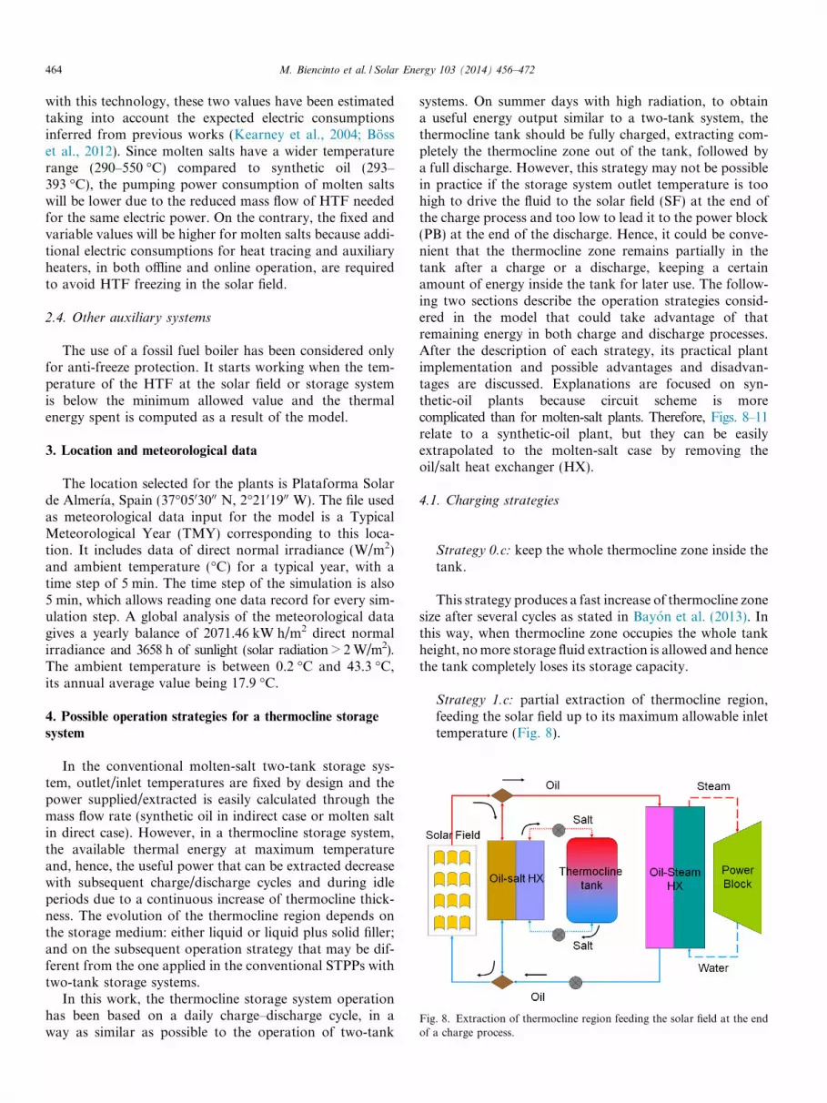
Fig. 8. Extraction of thermocline region feeding the solar field at the endof a charge process.


with this technology, these two values have been estimatedtaking into account the expected electric consumptionsinferred from previous works (Kearney et al., 2004; Bosset al., 2012). Since molten salts have a wider temperaturerange (290–550 �C) compared to synthetic oil (293–393 �C), the pumping power consumption of molten saltswill be lower due to the reduced mass flow of HTF neededfor the same electric power. On the contrary, the fixed andvariable values will be higher for molten salts because addi-tional electric consumptions for heat tracing and auxiliaryheaters, in both offline and online operation, are requiredto avoid HTF freezing in the solar field.

2.4. Other auxiliary systems

The use of a fossil fuel boiler has been considered onlyfor anti-freeze protection. It starts working when the tem-perature of the HTF at the solar field or storage systemis below the minimum allowed value and the thermalenergy spent is computed as a result of the model.

3. Location and meteorological data

The location selected for the plants is Plataforma Solarde Almerıa, Spain (37�0503000 N, 2�2101900 W). The file usedas meteorological data input for the model is a TypicalMeteorological Year (TMY) corresponding to this loca-tion. It includes data of direct normal irradiance (W/m2)and ambient temperature (�C) for a typical year, with atime step of 5 min. The time step of the simulation is also5 min, which allows reading one data record for every sim-ulation step. A global analysis of the meteorological datagives a yearly balance of 2071.46 kW h/m2 direct normalirradiance and 3658 h of sunlight (solar radiation > 2 W/m2).The ambient temperature is between 0.2 �C and 43.3 �C,its annual average value being 17.9 �C.

4. Possible operation strategies for a thermocline storage

system

In the conventional molten-salt two-tank storage sys-tem, outlet/inlet temperatures are fixed by design and thepower supplied/extracted is easily calculated through themass flow rate (synthetic oil in indirect case or molten saltin direct case). However, in a thermocline storage system,the available thermal energy at maximum temperatureand, hence, the useful power that can be extracted decreasewith subsequent charge/discharge cycles and during idleperiods due to a continuous increase of thermocline thick-ness. The evolution of the thermocline region depends onthe storage medium: either liquid or liquid plus solid filler;and on the subsequent operation strategy that may be dif-ferent from the one applied in the conventional STPPs withtwo-tank storage systems.

In this work, the thermocline storage system operationhas been based on a daily charge–discharge cycle, in away as similar as possible to the operation of two-tank

systems. On summer days with high radiation, to obtaina useful energy output similar to a two-tank system, thethermocline tank should be fully charged, extracting com-pletely the thermocline zone out of the tank, followed bya full discharge. However, this strategy may not be possiblein practice if the storage system outlet temperature is toohigh to drive the fluid to the solar field (SF) at the end ofthe charge process and too low to lead it to the power block(PB) at the end of the discharge. Hence, it could be conve-nient that the thermocline zone remains partially in thetank after a charge or a discharge, keeping a certainamount of energy inside the tank for later use. The follow-ing two sections describe the operation strategies consid-ered in the model that could take advantage of thatremaining energy in both charge and discharge processes.After the description of each strategy, its practical plantimplementation and possible advantages and disadvan-tages are discussed. Explanations are focused on syn-thetic-oil plants because circuit scheme is morecomplicated than for molten-salt plants. Therefore, Figs. 8–11relate to a synthetic-oil plant, but they can be easilyextrapolated to the molten-salt case by removing theoil/salt heat exchanger (HX).

4.1. Charging strategies

Strategy 0.c: keep the whole thermocline zone inside thetank.

This strategy produces a fast increase of thermocline zonesize after several cycles as stated in Bayon et al. (2013). Inthis way, when thermocline zone occupies the whole tankheight, no more storage fluid extraction is allowed and hencethe tank completely loses its storage capacity.

Strategy 1.c: partial extraction of thermocline region,feeding the solar field up to its maximum allowable inlettemperature (Fig. 8).


This is the simplest strategy, which in principle does notrequire any circuit modification. However, it is necessary tocontrol the SF outlet temperature by increasing the HTFflow or by defocusing some collector loops. Since part ofthe thermocline region remains within the tank, the storagecannot be fully charged and hence the overall energyobtained in the subsequent discharge will be lower thanin the two-tank case. To minimize this effect, the allowedSF inlet temperature, here fixed to 350 �C (see Table 1),could be increased, but this would require revising somecircuit components like HTF pumps, valves, expansion ves-sel, etc. In order to avoid control problems, the conditionfor stopping the charge process must be established fortank outlet temperature rather than for SF inlet tempera-ture. Therefore, the maximum allowed temperature of thefluid exiting the storage tank should be carefully selectedto guarantee that the maximum value at the SF inlet isnot attained.

Strategies 2.c and 3.c: total extraction of thermoclineregion, feeding, firstly, the solar field (Fig. 8) and, sec-ondly, the power block (Fig. 9).

These strategies imply an additional step to Strategy 1.cin order to extract the remaining thermocline region, whichallows the storage system to start the subsequent dischargeprocess from a situation of full storage charge. In this newstep, the remaining thermocline region is intended to feedthe PB and hence the minimum inlet temperature of HTFto PB (310 �C for oil SF and 430 �C for molten salts SF)should be lower than the maximum SF inlet temperature(here assumed to be 350 �C). This occurs in a synthetic-oil SF plant but not in a molten-salt SF plant (see Table 1).A better option can be to remove the remaining thermo-cline zone at low mass flow rate and mix it with the SFfluid, so that the mixture will reach the PB with enoughtemperature-but still lower than nominal, resulting in adecrease of both thermal power and cycle efficiency. Thisoption can be performed in two ways: either the storage

Fig. 9. Extraction of thermocline region feeding the power block at theend of a charge process.

system outlet flow is mixed with SF fluid at a constant massflow rate (Strategy 2.c) or both flows are regulated accord-ing to a required mixing temperature (Strategy 3.c). Byapplying Strategy 3.c, plant operability is improved andthe impact on both thermal power and cycle efficiency islower than applying Strategy 2.c. On the other hand, ther-mocline region will be extracted slower under Strategy 3.cthan under Strategy 2.c, with all the associated inconve-niences such us higher pumping power consumption, riskof an incomplete charge process, etc. For both strategiesa bypass is required (see Fig. 9) and this will imply the pres-ence of additional piping and valves to connect the storagesystem outlet with the PB inlet.

4.2. Discharging strategies

Strategy 0.d: keep the whole thermocline zone inside thetank.

As in a charge process, this strategy will produce a fastdegradation of thermocline zone size as stated in Bayonet al. (2013) and the tank will lose its storage capacity afterseveral charge/discharge cycles (in the same way as Strat-egy 0.c).

Strategy 1.d: partial extraction of thermocline region,feeding the power block down to the minimum allow-able temperature (Fig. 10).

This is the simplest strategy, which does not require anychange in the circuit. However, it has the drawback thatnot all stored energy is “well-spent”, since there is a partthat is used neither for PB nor SF. Furthermore, theremaining thermocline region expands overnight, due tothermal diffusion (Bayon and Rojas, 2013b). In principlethis should not affect the electric output of the plant, butit could give some operational problems after a time (forexample, an increase of tank outlet temperature in the sub-sequent charge process).

Fig. 10. Extraction of thermocline region feeding the power block at theend of a discharge process.


Strategies 2.d, 3.d and 4.d: total extraction of thermo-cline region, feeding, firstly, the power block (Fig. 10)and, secondly, the solar field (Fig. 11).

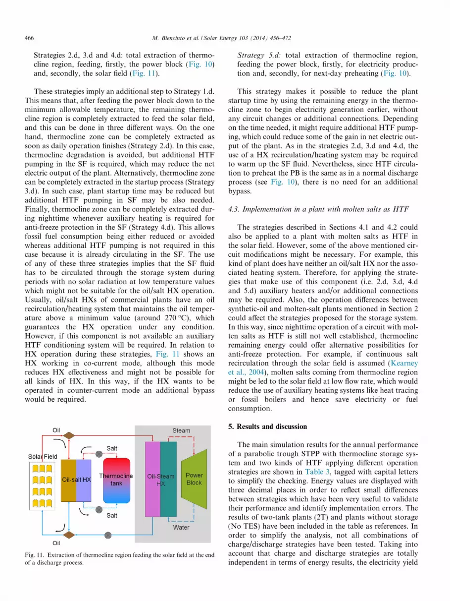
These strategies imply an additional step to Strategy 1.d.This means that, after feeding the power block down to theminimum allowable temperature, the remaining thermo-cline region is completely extracted to feed the solar field,and this can be done in three different ways. On the onehand, thermocline zone can be completely extracted assoon as daily operation finishes (Strategy 2.d). In this case,thermocline degradation is avoided, but additional HTFpumping in the SF is required, which may reduce the netelectric output of the plant. Alternatively, thermocline zonecan be completely extracted in the startup process (Strategy3.d). In such case, plant startup time may be reduced butadditional HTF pumping in SF may be also needed.Finally, thermocline zone can be completely extracted dur-ing nighttime whenever auxiliary heating is required foranti-freeze protection in the SF (Strategy 4.d). This allowsfossil fuel consumption being either reduced or avoidedwhereas additional HTF pumping is not required in thiscase because it is already circulating in the SF. The useof any of these three strategies implies that the SF fluidhas to be circulated through the storage system duringperiods with no solar radiation at low temperature valueswhich might not be suitable for the oil/salt HX operation.Usually, oil/salt HXs of commercial plants have an oilrecirculation/heating system that maintains the oil temper-ature above a minimum value (around 270 �C), whichguarantees the HX operation under any condition.However, if this component is not available an auxiliaryHTF conditioning system will be required. In relation toHX operation during these strategies, Fig. 11 shows anHX working in co-current mode, although this modereduces HX effectiveness and might not be possible forall kinds of HX. In this way, if the HX wants to beoperated in counter-current mode an additional bypasswould be required.

Fig. 11. Extraction of thermocline region feeding the solar field at the endof a discharge process.

Strategy 5.d: total extraction of thermocline region,feeding the power block, firstly, for electricity produc-tion and, secondly, for next-day preheating (Fig. 10).

This strategy makes it possible to reduce the plantstartup time by using the remaining energy in the thermo-cline zone to begin electricity generation earlier, withoutany circuit changes or additional connections. Dependingon the time needed, it might require additional HTF pump-ing, which could reduce some of the gain in net electric out-put of the plant. As in the strategies 2.d, 3.d and 4.d, theuse of a HX recirculation/heating system may be requiredto warm up the SF fluid. Nevertheless, since HTF circula-tion to preheat the PB is the same as in a normal dischargeprocess (see Fig. 10), there is no need for an additionalbypass.

4.3. Implementation in a plant with molten salts as HTF

The strategies described in Sections 4.1 and 4.2 couldalso be applied to a plant with molten salts as HTF inthe solar field. However, some of the above mentioned cir-cuit modifications might be necessary. For example, thiskind of plant does have neither an oil/salt HX nor the asso-ciated heating system. Therefore, for applying the strate-gies that make use of this component (i.e. 2.d, 3.d, 4.dand 5.d) auxiliary heaters and/or additional connectionsmay be required. Also, the operation differences betweensynthetic-oil and molten-salt plants mentioned in Section 2could affect the strategies proposed for the storage system.In this way, since nighttime operation of a circuit with mol-ten salts as HTF is still not well established, thermoclineremaining energy could offer alternative possibilities foranti-freeze protection. For example, if continuous saltrecirculation through the solar field is assumed (Kearneyet al., 2004), molten salts coming from thermocline regionmight be led to the solar field at low flow rate, which wouldreduce the use of auxiliary heating systems like heat tracingor fossil boilers and hence save electricity or fuelconsumption.

5. Results and discussion

The main simulation results for the annual performanceof a parabolic trough STPP with thermocline storage sys-tem and two kinds of HTF applying different operationstrategies are shown in Table 3, tagged with capital lettersto simplify the checking. Energy values are displayed withthree decimal places in order to reflect small differencesbetween strategies which have been very useful to validatetheir performance and identify implementation errors. Theresults of two-tank plants (2T) and plants without storage(No TES) have been included in the table as references. Inorder to simplify the analysis, not all combinations ofcharge/discharge strategies have been tested. Taking intoaccount that charge and discharge strategies are totallyindependent in terms of energy results, the electricity yield

Table 3Main simulation results for the annual performance of STPPs with no storage (No TES), two-tank storage (2T) and thermocline storage (TC), and twokinds of HTF (synthetic oil and molten salt), including gross and net electricity yield, fossil energy required, total operation time (in hours) and averagestartup time (in minutes) of the power block (PB) and maximum solar field (SF) inlet temperature obtained from annual simulations.

Plant type Combinationtag

Chargestrategy

Dischargestrategy

Gross electricityyield (GW he)

Net electricityyield (GW he)

Fossil thermalenergy (GW ht)

PBoperationtime (h)

PB startuptime (min)

Max Tin

SF (�C)

Synthetic oil as HTF

Oil 2-Tank 2T – – 161.995 142.049 9.224 3672.7 74.3 293.7Oil No TES No TES – – 114.540 99.522 10.529 2728.8 81.7 293.7Oil TC 0 0.c 0.d 114.638 99.662 10.144 2726.1 81.8 293.7Oil TC A 1.c 1.d 158.629 138.610 9.344 3686.0 74.6 346.0Oil TC B 1.c 2.d 158.497 138.416 7.823 3683.5 74.7 346.0Oil TC C 1.c 3.d 158.640 138.616 9.299 3686.3 74.6 346.0Oil TC D 1.c 4.d 158.434 138.402 7.244 3681.6 74.7 346.0Oil TC E 1.c 5.d 158.941 138.901 9.298 3685.7 72.5 346.0Oil TC A* 1.c 1.d 158.428 138.459 9.336 3680.8 74.6 315.3Oil TC F* 2.c 1.d 158.358 138.352 9.347 3685.9 74.6 315.3Oil TC G* 3.c 1.d 158.446 138.405 9.342 3685.0 74.6 315.3

Molten salts as HTF

MS 2-Tank 2T – – 146.666 133.352 45.646 3358.9 65.5 294.0MS No TES No TES – – 106.624 95.320 67.594 2483.9 66.6 294.0MS TC 0 0.c 0.d 106.641 95.342 68.379 2482.2 67.0 294.0MS TC A 1.c 1.d 144.686 131.439 61.539 3331.9 66.6 347.3MS TC B 1.c 2.d 144.718 131.470 57.852 3333.7 66.7 348.3MS TC C 1.c 3.d 144.479 131.235 61.514 3335.6 69.1 348.7MS TC D 1.c 4.d 144.468 131.229 56.156 3325.6 66.6 349.5MS TC E 1.c 5.d 144.850 131.520 61.537 3331.8 65.4 349.7MS TC F 2.c 1.d 144.409 131.156 61.525 3332.8 66.6 347.2MS TC G 3.c 1.d 144.672 131.385 61.566 3334.2 66.6 348.2


of a certain combination of strategies can be obtained justadding the gain of each strategy with respect to the basecase A (1.c,1.d). For example, the total yield of the combi-nation (3.c,3.d) will be the sum of the (1.c,1.d) yield plusthe gain of (3.c,1.d) and (1.c,3.d) with respect to the(1.c,1.d) case.

For the reference two-tank plants (2T) we observe thatthe value of net electricity yield for a molten-salt plant is8.7 GW he lower than for a synthetic-oil plant. This differ-ence is associated to the high freezing temperature of thesalt, which limits the operation conditions for the powerblock. This limitation is reflected in the power block oper-ating hours, which is 313.8 h less for the molten-salt plant.Therefore, despite the higher nominal power block effi-ciency of a molten-salt plant, the annual net electricity yieldresults to be lower than the yield of a synthetic-oil plant.Additionally, the anti-freeze protection requires salt recir-culation during night and auxiliary heating with fossil fuel.This is why the fossil fuel consumption of a molten-saltplant is considerably higher (around 5 times) than the syn-thetic-oil plant consumption.

In terms of strategies with thermocline storage systems,the results of combination 0 (0.c + 0.d strategies) in bothsynthetic-oil and molten-salt plants are similar to those ofplants without thermal storage (No TES configurations).This is due to the quick degradation of thermocline zone(Bayon et al., 2013) if no extraction strategy is applied,which makes this zone to occupy half of tank height in less

than 4 days (i.e. the storage capacity is reduced to 50%).When thermocline zone occupies the whole tank, the systemcompletely loses its storage capacity because the operationstrategy does not allow any extraction of thermocline region.Therefore, the energy sent to the storage system is dumpedalmost all days of the year and the annual yield gain of thiscombination compared to the ‘No TES’ case is negligible.

For the case of synthetic-oil plants, the simulations con-sidering charge strategies 2.c and 3.c are not shown inTable 3 since they produce identical annual performanceresults as Strategy 1.c. These identical results come fromthe fact that, if maximum allowed SF inlet temperatureof 350 �C is imposed, thermocline zone is totally extractedbefore this limit has been reached. In contrast, for the caseof molten-salt plants, the simulations considering chargestrategies 1.c, 2.c and 3.c lead to different annual perfor-mance results when 350 �C is established as the maximumallowed inlet temperature to the solar field and, thus, theircorresponding simulation results are shown in Table 3.

In order to assess and compare charge strategies 1.c, 2.cand 3.c in synthetic-oil plants, a lower limit for the allowedsolar field inlet temperature has also been tested (315 �C)with discharge Strategy 1.d. The corresponding combina-tions have been marked with an asterisk (*) in Table 3. Inthese cases, although annual performance results are quitesimilar, they are different, so they will be used for compar-ing these three charge strategies in synthetic-oil plants. Itcan be seen that annual net electricity yield (6th column


in Table 3) obtained for Strategy 1.c, for either synthetic-oil(combination A*) or molten-salt plants (combination A), ishigher than for charging strategies 2.c (combinations F* orF, respectively) and for 3.c (combinations G* or G, respec-tively). As expected, Strategy 3.c (combinations G* and G)gives better results than Strategy 2.c (combinations F* andF). In order to understand the differences observed inannual net electricity yield, the corresponding net electricpower, electric power losses, stored energy and solar irradi-ance curves have been plotted in Fig. 12 for a typical sum-mer day in the case of synthetic-oil plants. In this figure, netelectric power has different types of fluctuations when stor-age becomes full, depending on the charge strategy. Forcharge Strategy 2.c (combination F*) there is a deep andnarrow decrease coming from a sudden decrease of thetemperature of the flow feeding the power block. Nominalpower generation conditions are quickly achieved. ChargeStrategy 3.c (combination G*) has a smaller decrease, sinceextraction of the thermocline zone is controlled to obtainas close nominal inlet temperature to PB as possible, buttakes more time (extracting the thermocline region takeslonger), thus pumping power consumption during thermo-cline extraction is higher.

Fig. 12. Simulation results of the three charge strategies (combinations A*

As we can see, the electricity yield (gross and net) resultsfor a thermocline storage system are always lower than theresults for a two-tank system. As said before, this happensbecause, despite both cases have the same storage capacity(see Table 1), thermocline tanks develop a temperatureprofile that diminishes the available thermal energy at max-imum temperature, and hence the useful energy that can beextracted. In Fig. 13 (synthetic-oil STPP) and Fig. 14(molten-salt STPP), the difference between the results of atwo-tank system and a thermocline one are depicted forall the strategy combinations of Table 3. The operationstrategies are arranged in qualitative order of complexity(in terms of circuit modifications and control mechanisms).Although the differences among combinations are quitelow, combination E (Figs. 13 and 14, left) leads to thelowest yield difference and hence to the best net electricoutput (see Table 3) with a thermocline system. It yields291 MW he more than the base combination (i.e., A) inthe case of synthetic-oil plants and 81 MW he in the caseof molten-salt plants. This is mainly due to a lower meanstartup time of the power block, with 2.1 min differencerelated to the A case for synthetic-oil plants and 1.2 minfor molten-salt ones.

, F*, G*) for a typical summer day in the case of a synthetic-oil STPP.

Fig. 13. Annual electricity yield decrease and fossil energy increase for each strategy combination with respect to the two-tank system, in the case ofsynthetic-oil STPPs.

Fig. 14. Annual electricity yield decrease and fossil energy increase for each strategy combination with respect to the two-tank system, in the case ofmolten-salt STPPs.


In terms of fossil fuel consumption, combinations B andD for synthetic-oil plants (Fig. 13, right) show a fossilenergy saving of 1.4 GW ht (15.2%) for B and 2 GW ht

(21.5%) for D comparing with the reference two-tank case.Taking into account the calorific value of natural gas(39,900 kJ/kg), the application of these strategies couldrepresent gas savings of 126.3 t and 178.6 t, respectively.In the case of molten-salt plants (Fig. 14, right) the fossilfuel consumption of a thermocline storage system is alwayshigher than for the reference two-tank system. In any typeof STPP with thermocline storage, strategies of combina-tions B and D show the lowest fossil fuel consumption.The fossil energy saving is associated to the moment atwhich each strategy uses the thermocline remaining heat.A proper extraction of this energy may cause a delay (B)or reduction (D) in the need for fossil fuel that is requiredto avoid HTF freezing in solar field, for both synthetic-oiland molten-salt plants. In order to illustrate this effect,Fig. 15 displays some simulation results for each dischargestrategy during two consecutive typical summer days (onewith high radiation and one with medium) and their corre-sponding nights, for the case of synthetic-oil plants. Besidesthermal power obtained from thermocline extraction andfossil thermal power curves, Fig. 15 includes net electricpower, stored energy and solar irradiance curves. Combination

A shows that the solar field requires auxiliary heat supportduring nights organized in just one supply or peak beforethe first two summer days (let’s call them P1 and P2,respectively) and in two supplies or peaks (P3 and P4)before what the third day would be. When strategy combi-nation B is applied, two auxiliary supplies to SF (P1 andP4) are avoided. This suggests that feeding the SF just afterfinishing PB operation with the remaining thermoclineregion energy prevents the use of auxiliary SF heating sincefreezing conditions are more unlikely to happen. Theseconditions, if happened, are delayed in time and reducedin amount (P2 and P3). If the remaining energy of the ther-mocline region is given to the SF in the startup operation,just prior next day operation (combination C), there isnearly no effect on either auxiliary heating (see also Table 3)or startup time (only numerically visible by gross and netelectricity yield in Table 3). With combination D the ther-mocline remaining energy is addressed to the SF whenfreezing conditions are achieved, thus placing in the sametime position, auxiliary consumptions for SF are reduced.

As said above, for the case of molten-salt plants, the fos-sil fuel consumption in a thermocline storage system ishigher than in a two-tank system. Even so, the fossil fuelsaving of the mentioned two strategies with respect to thebase strategy (A) is remarkable, 3.7 GW ht (6%) for B

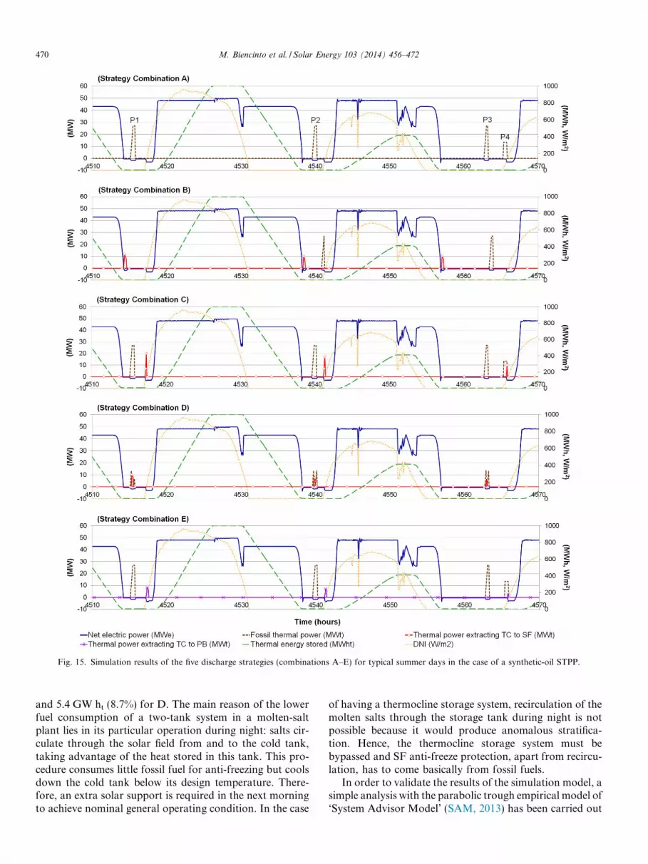
Fig. 15. Simulation results of the five discharge strategies (combinations A–E) for typical summer days in the case of a synthetic-oil STPP.


and 5.4 GW ht (8.7%) for D. The main reason of the lowerfuel consumption of a two-tank system in a molten-saltplant lies in its particular operation during night: salts cir-culate through the solar field from and to the cold tank,taking advantage of the heat stored in this tank. This pro-cedure consumes little fossil fuel for anti-freezing but coolsdown the cold tank below its design temperature. There-fore, an extra solar support is required in the next morningto achieve nominal general operating condition. In the case

of having a thermocline storage system, recirculation of themolten salts through the storage tank during night is notpossible because it would produce anomalous stratifica-tion. Hence, the thermocline storage system must bebypassed and SF anti-freeze protection, apart from recircu-lation, has to come basically from fossil fuels.

In order to validate the results of the simulation model, asimple analysis with the parabolic trough empirical model of‘System Advisor Model’ (SAM, 2013) has been carried out


for the reference two-tank (2T) and no storage (No TES)cases with both HTFs, applying the specifications includedin Table 1. The net annual electricity yield obtained withSAM for synthetic oil is 142.5 GW he in the two-tank caseand 102.3 GW he in the ‘No TES’ case (vs. 142.0 GW he

and 99.5 GW he, respectively, shown in Table 3), while formolten salts it is 122.4 GW he in the two-tank case and95.8 GW he in the ‘No TES’ case (vs. 133.4 GW he and95.3 GW he, respectively, shown in Table 3). In general,the SAM figures are in good agreement with the results dis-played in Table 3 except for the case of a two-tank systemusing molten salts as HTF, which presents 9% lower netannual yield. Additionally, the thermal energy used foranti-freeze protection with molten salts as HTF is signifi-cantly lower for the case of SAM simulation (18.4 GW ht)than for the present study (45.6 GW ht). These differencesmay be associated to the specific operation strategy consid-ered for anti-freeze protection of molten salts using atwo-tank system developed in our model and described inSection 2, which is not included in SAM model. Actually,this strategy for anti-freeze protection seems to improvethe net annual yield (133.4 GW he vs. 122.4 GW he), whichcould indicate that the additional thermal energy used foranti-freezing helps reducing both SF and PB startup times,although the continuous fluid recirculation is expected toincrease pumping power consumption.

This study has proved that the annual electricity yield of athermocline storage system is always lower than the annualyield of a two-tank system for both kinds of HTF (syntheticoil and molten salts). Nevertheless, the expected cost reduc-tion associated to both a single tank construction and thedecrease of molten salts inventory due to the presence of asolid filler material should be taken into account. Addition-ally, the country in which the plant is going to be installedand its financial conditions will determine the electricityprice and fossil fuel cost and hence the total thermal storagebudget. In this way, the results of Table 3, Figs. 13 and 14can be used as a guideline for the economic comparison ofannual electricity yield and fossil fuel consumption for eachoperation strategy with respect to a two-tank system.

6. Conclusions

An annual performance analysis has been carried outfor different operation strategies regarding charge and dis-charge processes that could be applied to a thermoclinestorage system integrated in parabolic trough STPPs, usingeither synthetic oil or molten salts as HTF. The results havebeen compared with the ones obtained for plants with atwo-tank storage system, where only one operation strat-egy is considered, according to the information receivedfrom commercial plants.

This study has proved that the annual electricity yield ofa STPP with a thermocline tank is always lower than theyield of the same plant with a two-tank system. In generalterms, the electricity yield and fossil fuel consumption ofthe seven analyzed strategies show a similar behavior for

synthetic oil and also for molten salts. This means thatthe best strategies could be the same for both kinds of heattransfer fluids.

It has been found that the best strategy for charge pro-cesses in terms of annual electricity yield and fossil fuelconsumption is a partial extraction of thermocline region,feeding the solar field up to its maximum allowable inlettemperature. This strategy presents the additional advan-tage that it is the simplest one to implement in a parabolictrough STPP.

In terms of annual electricity yield, the best strategy fordischarge processes is a total extraction of thermoclineregion, feeding the power block, firstly, for electricity pro-duction and, secondly, for the next day preheating. Thisstrategy is easy to implement in a parabolic trough STPPand does not require more fossil consumption than keepingthe remaining energy inside the tank. However, the annualnet electricity gain of the best strategy is not verysignificant.

In terms of annual fossil fuel consumption, the beststrategy for discharge processes is a total extraction of ther-mocline region, feeding, firstly, the power block and, sec-ondly, the solar field during nighttime whenever auxiliaryheating is required for anti-freeze protection. This strategypresents an intermediate complexity in terms of plantimplementation but leads to a lower annual electricity yieldthan other strategies.

From a global viewpoint, the convenience of using athermocline tank with direct (molten salts as HTF) orindirect storage (synthetic oil as HTF), instead of atwo-tank system, and the choice of the best strategy forthe corresponding parabolic trough plant would requirea further economic assessment. The economic scenarioin terms of electricity prices, fossil fuel cost and materialand building costs, together with energy policies andfinancial conditions of the location in which the plant isgoing to be installed, will strongly determine not onlythe best plant configuration but also the optimum opera-tion strategy.

Acknowledgements

The authors would like to acknowledge the E.U.through the 7th Framework Programme for the financialsupport of this work under the O.P.T.S. project with con-tract number: 283138.

References

Bayon, R., Rojas, E., 2013a. Simulation of thermocline storage for solarthermal power plants: from dimensionless results to prototypes andreal size tanks. Int. J. Heat Mass Transf. 60, 713–721.

Bayon, R., Rojas, E., 2013b. Analytical description of thermocline tankperformance in dynamic processes and stand-by periods. In: 2013 ISESSolar World Congress, Cancun, Mexico.

Bayon, R., Rojas, E., 2014. Analytical function describing the behaviourof a thermocline storage tank: a requirement for annual simulations ofsolar thermal power plants. Int. J. Heat Mass Transf. 68, 641–648.

http://refhub.elsevier.com/S0038-092X(14)00125-X/h0005







Bayon, R., Rojas, E., Rivas, E., 2013. Study of thermocline tankperformance in dynamic processes and stand-by periods with ananalytical function. In: SolarPACES 2013 Conference, Las Vegas,USA.

Biencinto, M., Gonzalez, L., Zarza, E., Dıez, L.E., Munoz, J., Martınez-Val, J.M., 2012. Modeling and Simulation of a Loop of ParabolicTroughs using Nitrogen as Working Fluid. In: SolarPACES 2012Conference, Marrakech, Morocco.

Boss, F., Fluri, T.P., Branke, R., Platzer, W.J., 2012. Simulation ofparabolic trough power plants with molten salt as heat transfer fluid.In: SolarPACES 2012 Conference, Marrakech, Morocco.

Eickhoff, M., Steinbach, S., Luepfert, E., 2001. Collector Efficiencies ofthe EuroTrough-Collector. EuroTrough-II Project Task Report,European Commission Contract ERK6-CT1999-00018, PlataformaSolar de Almerıa, Spain.

Flueckiger, S.M., Iverson, B.D., Garimella, S.V., 2013. Economicoptimization of a concentrating solar power plant with molten-saltthermocline storage. J. Sol. Energy Eng. 136 (1), 011016.

Flueckiger, S.M., Iverson, B.D., Garimella, S.V., Pacheco, J.E., 2014.System-level simulation of a solar power tower plant with thermoclinethermal energy storage. Appl. Energy 113, 86–96.

Gonzalez, L., Biencinto, M., 2012. Validacion del modelo de simulacionde la central termosolar La Florida. CIEMAT-PSA Internal Report,Doc. Id: USSC-SC-QA-67.

IRENA, 2012. Concentrating solar power, In: Renewable energy tech-nologies: cost analysis series, vol. 1: Power Sector, IRENA Secretariat,Abu Dhabi, United Arab Emirates, issue 2/5, pp. 1–48.

Kearney, D., Herrmann, U., Nava, P., Kelly, B., Mahoney, R., Pacheco,J., Cable, R., Potrovitza, N., Blake, D., Price, H., 2003. Assessment ofa molten salt heat transfer fluid in a parabolic trough solar field. J.Sol.Energy Eng. 125 (2), 170–176.

Kearney, D., Kelly, B., Herrmann, U., Cable, R., Pacheco, J., Mahoney,R., Price, H., Blake, D., Nava, P., Potrovitza, N., 2004. Engineeringaspects of a molten salt heat transfer fluid in a trough solar field.Energy 29, 861–870.

Kolb, G., 2011. Evaluation of annual performance of 2-tank andthermocline thermal storage systems for trough plants. J. Sol. EnergyEng. 133 (3), 031023.

Kolb, G., Hassani, V., 2006. Performance Analysis of Thermocline EnergyStorage Proposed for the 1 MW Saguaro Solar Trough Plant. In:Proceedings of ISEC 2006, ASME International Solar Energy Con-ference, Denver, USA.

Kosman, G., Rusin, A., 2001. The influence of the start-ups and cyclicloads of steam turbines conducted according to European standardson the component’s life. Energy 26 (2001), 1083–1099.

Libby, C., 2010. Solar thermocline storage systems: preliminary designstudy. EPRI, Palo Alto, CA, USA, 1019581.

Libby, C., Cerezo, L., Bedilion, R., Pietruszkiewicz, J., Lamar, M.,Hollenbach, R., 2010b. Design of high temperature solar thermoclinestorage systems. In: SolarPACES 2010 Conference, Perpignan, France.

Muller-Elvers, C., Wittmann, M., Saur, M., 2012. Design and Construc-tion of Molten Salt Parabolic Trough HPS Project in Evora, Portugal.In: SolarPACES 2012 Conference, Marrakech, Morocco.

Nithyanandam, K., Pitchumani, R., 2014. Cost and performance analysisof concentrating solar power systems with integrated latent thermalenergy storage. Energy 64, 793–810.

Pacheco, J.E., Showalter, S.K., Kolb, W.J., 2002. Development of amolten-salt thermocline thermal storage system for parabolic troughplants. J. Sol. Energy Eng. 124 (2), 153–159.

Relloso, S., Delgado, E., 2009. Experience with molten salts thermalstorage in a commercial parabolic trough plant. Andasol-1 commis-sioning and operation. In: SolarPACES 2009 Conference, Berlin,Germany.

SAM, 2013. System Advisor Model Version 2013.1.15 (SAM 2013.1.15).Available from: <https://sam.nrel.gov/content/downloads>. NationalRenewable Energy Laboratory. Golden, CO, USA (accessed 18.10.13).

Siemens, A.G., 2011. Steam turbines for CSP plants. Available from:<http://www.energy.siemens.com/hq/en/renewable-energy/solar-power/csp-steam-turbine.htm> Siemens AG, Energy Sector, Erlangen,Germany (accessed 03.10.13).

TRNSYS�, 2007. Volume 8: Programmer’s Guide, in: TRNSYS� 16, aTransient System Simulation Program. Solar Energy Laboratory,University of Wisconsin-Madison, USA.

Wittmann, M., Eck, M., Pitz-Paal, R., Muller-Steinhagen, H., 2011.Methodology for optimized operation strategies of solar thermalpower plants with integrated heat storage. Sol. Energy 85 (4), 653–659.





























https://sam.nrel.gov/content/downloads

http://www.energy.siemens.com/hq/en/renewable-energy/solar-power/csp-steam-turbine.htm

http://www.energy.siemens.com/hq/en/renewable-energy/solar-power/csp-steam-turbine.htm




Simulation and assessment of operation strategies for solar thermal power plants with a thermocline...

Documents

Transcript of Simulation and assessment of operation strategies for solar thermal power plants with a thermocline...