A wavelet-based variability model (WVM) for solar PV power plants

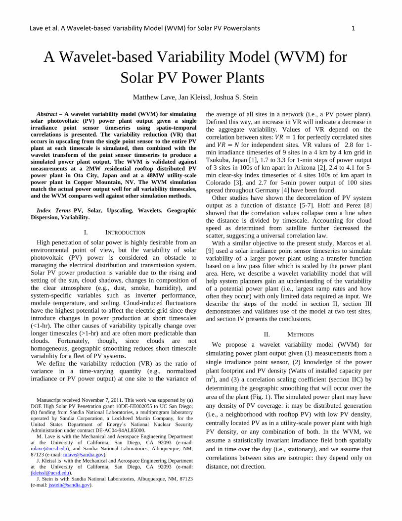
Lave et al. A Wavelet-based Variability Model (WVM) for Solar PV Powerplants 1

A Wavelet-based Variability Model (WVM) for

Solar PV Power Plants Matthew Lave, Jan Kleissl, Joshua S. Stein

Abstract – A wavelet variability model (WVM) for simulating

solar photovoltaic (PV) power plant output given a single

irradiance point sensor timeseries using spatio-temporal

correlations is presented. The variability reduction (VR) that

occurs in upscaling from the single point sensor to the entire PV

plant at each timescale is simulated, then combined with the

wavelet transform of the point sensor timeseries to produce a

simulated power plant output. The WVM is validated against

measurements at a 2MW residential rooftop distributed PV

power plant in Ota City, Japan and at a 48MW utility-scale

power plant in Copper Mountain, NV. The WVM simulation

match the actual power output well for all variability timescales,

and the WVM compares well against other simulation methods.

Index Terms–PV, Solar, Upscaling, Wavelets, Geographic

Dispersion, Variability.

I. INTRODUCTION

High penetration of solar power is highly desirable from an

environmental point of view, but the variability of solar

photovoltaic (PV) power is considered an obstacle to

managing the electrical distribution and transmission system.

Solar PV power production is variable due to the rising and

setting of the sun, cloud shadows, changes in composition of

the clear atmosphere (e.g., dust, smoke, humidity), and

system-specific variables such as inverter performance,

module temperature, and soiling. Cloud-induced fluctuations

have the highest potential to affect the electric grid since they

introduce changes in power production at short timescales

(<1-hr). The other causes of variability typically change over

longer timescales (>1-hr) and are often more predictable than

clouds. Fortunately, though, since clouds are not

homogeneous, geographic smoothing reduces short timescale

variability for a fleet of PV systems.

We define the variability reduction (VR) as the ratio of

variance in a time-varying quantity (e.g., normalized

irradiance or PV power output) at one site to the variance of

the average of all sites in a network (i.e., a PV power plant).

Defined this way, an increase in VR will indicate a decrease in

the aggregate variability. Values of VR depend on the

correlation between sites: for perfectly correlated sites

and for independent sites. VR values of 2.8 for 1-

min irradiance timeseries of 9 sites in a 4 km by 4 km grid in

Tsukuba, Japan [1], 1.7 to 3.3 for 1-min steps of power output

of 3 sites in 100s of km apart in Arizona [2], 2.4 to 4.1 for 5-

min clear-sky index timeseries of 4 sites 100s of km apart in

Colorado [3], and 2.7 for 5-min power output of 100 sites

spread throughout Germany [4] have been found.

Other studies have shown the decorrelation of PV system

output as a function of distance [5-7]. Hoff and Perez [8]

showed that the correlation values collapse onto a line when

the distance is divided by timescale. Accounting for cloud

speed as determined from satellite further decreased the

scatter, suggesting a universal correlation law.

With a similar objective to the present study, Marcos et al.

[9] used a solar irradiance point sensor timeseries to simulate

variability of a larger power plant using a transfer function

based on a low pass filter which is scaled by the power plant

area. Here, we describe a wavelet variability model that will

help system planners gain an understanding of the variability

of a potential power plant (i.e., largest ramp rates and how

often they occur) with only limited data required as input. We

describe the steps of the model in section II, section III

demonstrates and validates use of the model at two test sites,

and section IV presents the conclusions.

II. METHODS

We propose a wavelet variability model (WVM) for

simulating power plant output given (1) measurements from a

single irradiance point sensor, (2) knowledge of the power

plant footprint and PV density (Watts of installed capacity per

m2), and (3) a correlation scaling coefficient (section IIC) by

determining the geographic smoothing that will occur over the

area of the plant (Fig. 1). The simulated power plant may have

any density of PV coverage: it may be distributed generation

(i.e., a neighborhood with rooftop PV) with low PV density,

centrally located PV as in a utility-scale power plant with high

PV density, or any combination of both. In the WVM, we

assume a statistically invariant irradiance field both spatially

and in time over the day (i.e., stationary), and we assume that

correlations between sites are isotropic: they depend only on

distance, not direction.

Manuscript received November 7, 2011. This work was supported by (a)

DOE High Solar PV Penetration grant 10DE-EE002055 to UC San Diego; (b) funding from Sandia National Laboratories, a multiprogram laboratory

operated by Sandia Corporation, a Lockheed Martin Company, for the

United States Department of Energy’s National Nuclear Security Administration under contract DE-AC04-94AL85000.

M. Lave is with the Mechanical and Aerospace Engineering Department

at the University of California, San Diego, CA 92093 (e-mail: [email protected]), and Sandia National Laboratories, Albuquerque, NM,

87123 (e-mail: [email protected]).

J. Kleissl is with the Mechanical and Aerospace Engineering Department at the University of California, San Diego, CA 92093 (e-mail:

[email protected]).

J. Stein is with Sandia National Laboratories, Albuquerque, NM, 87123 (e-mail: [email protected]).

mailto:[email protected]





The WVM is designed to provide simulated power plant

output to grid integration studies which test the effects of

adding PV to existing electric feeders. These studies are done

historically, after load and irradiance have been measured, and

show the potential impacts of PV variability had PV been

installed on the feeder being studied.

While the WVM is not a stand-alone forecasting model, it

could be integrated into forecasting methods if spatially-

distributed forecasted irradiances were available at high

temporal resolution. However, satellite and numerical weather

prediction forecast models typically only output at a temporal

resolution of 30 minutes such that an upscaling method such

as the WVM is not required since essentially no geographic

smoothing occurs over power plant length scales (O~10 km) at

such long timescales.

The main steps to the WVM are detailed in the sections

below.

A. Wavelet Decomposition

We decompose the input irradiance point sensor timeseries

into its components at various timescales by using a wavelet

transform.

To obtain a stationary signal, the irradiance timeseries is

normalized such that output during clear conditions is 1.

( ) ( ) ( ), (1)

where ( ) is the normalized signal, and ( ) is

the clear-sky model (here the Ineichen model [10]). For

simplicity of notation, we here assume that the point sensor is

a global horizontal irradiance (GHI) sensor. If instead a plane

of array (POA) sensor were used, a POA clear-sky model

would be required.

The wavelet transform of the clear-sky index, ( ),

is:

( ) ∫ ( )

√ (

)

, (2)

where the wavelet timescale (duration of fluctuations) is ,

and designate the start and end of the GHI

timeseries, and is a variable of integration. For the discrete

wavelet transform, is increased by factors of 2, such that

values of are defined by . We used the top hat

wavelet, defined by:

( ) {

, (3)

because of its simplicity and similarity to the shape of solar

power fluctuations [11]. For 1-day at 1-sec resolution, we

compute wavelet modes (timeseries) for values ranging from

2-sec ( ) to 4096-sec ( ), thus decomposing the

( ) timeseries into 12 modes ( ) showing

fluctuations at these various timescales. Symmetric signal

extension is used to ensure resolution at endpoints. The largest

timescale over which correlations are considered is 4096 sec (j

= 12) because over the spatial scales of interest (O~10 km) the

amount of smoothing that occurs at longer time scales is

insignificant. In addition, modes for require such

significant signal extension that they are no longer

representative of true fluctuations in the irradiance timeseries.

We adopt a special definition for the highest wavelet mode,

defining ( ) to be the moving average with

window 4096-sec. By doing so, we achieve the property that

the sum of all wavelet modes equals the original input signal:

∑ ( ) ( ). (4)

B. Distances

We next discretize the power plant into individual ‘sites’. A

single site is chosen to be an area over which ( )

for the timescales of interest. For distributed plants, a single

site is one rooftop PV system. For utility-scale plants, a single

site is a small container of PV modules, as dictated by

computational limitations. When using larger containers, a

correction is applied for the in-container smoothing. Once

discrete sites have been defined, the distance between each

pair of sites is computed.

C. Correlations

To determine correlations between sites we assume that

correlation is a function of distance divided by timescale [8]:

( ) (

), (5)

where is the correlation between sites, is the distance

between sites and , is the timescale, and is a

correlation scaling factor. The value can be found using a

small network of irradiance sensors (at least ~4-6 sites) where

the correlations, distances, and timescales are known and

may be solved for using Eq. 5. The value varies day-by-day

and by location due to changing cloud speed. Smaller values

(1-3, typically observed at coastal sites with low, slow clouds)

result in lower correlations between sites, while large values

(>4, typical of inland sites with high, fast-moving clouds)

mean higher correlations. Through future work, we will create

a closed form solution where can be determined from

geographic and meteorological variables and multiple

irradiance sensors are not required.

Fig. 1. Diagram showing the inputs and outputs for the WVM.

PV Plant Footprint

Point Sensor Timeseries

Density of PV

WVM Inputs WVM Outputs

Plant Areal Average Irradiance

determine variability reduction (smoothing) at each wavelet timescale

Location/Day Dependent “ ”

Coefficient Plant Power Output

irradiance to power model


D. Variability Reduction

The variability reduction as a function of timescale, ( ),

is defined as the variance of the point sensor divided by the

variance of the entire PV power plant at each timescale. VR

can be expressed as the inverse of the average of all

correlations modeled in Eq. (5):

( )

∑ ∑ ( )

, (6)

where is the total number of sites. Defined this way,

for entirely independent sites ( ), and

for entirely dependent sites.

E. Simulate Wavelet Modes of Power plant

By combining the wavelet modes ( ) found in section

II.A with the variability reductions ( ) from section II.D,

we simulate the wavelet modes of the power plant. The

simulated wavelet modes of normalized power are reduced in

magnitude by the square root of VR:

( )

( )

√ ( ), (7)

where ( ) are the simulated power plant wavelet modes.

We can sum the simulated wavelet modes (inverse wavelet

transform) to create a simulated clear-sky index of area-

averaged over the power plant:

( ) ∑

( )

. (8)

F. Convert to Power Output

Power output is obtained by multiplying the spatially

averaged irradiance (section II.E) by a clear-sky power output

model, ( ) .

( ) ( ) ( ) (9)

( ) is created by combining a plane of array irradiance

clear-sky model with the plant’s capacity, , and a constant

conversion factor, .

( ) ( ) (10)

To obtain ( ) , we apply the Page Model [12] to

( ). Since the Page Model requires GHI and diffuse

irradiance as inputs, diffuse fraction was estimated as in [13].

The constant conversion factor, , is determined based on the

power plant’s conversion efficiency.

Since PV plant power output is nearly linearly proportional

to spatially averaged irradiance [14], using only a constant

multiplier ( ) is a reasonable approximation for this

application. In practice, though, more sophisticated

performance models [15] should be used that depend on

ambient temperature, wind speed, and module specifications.

The improvement in accuracy of power output achieved by

using such a non-linear model depends on how far variables

such as temperature deviate from standard test conditions

(STC), but is expected to usually be less than 10%. Errors in

estimating the variability at short timescales will be even

smaller, since most of the non-linear irradiance to power

effects occur over long timescales.

III. RESULTS/APPLICATION TO OTA CITY AND

COPPER MOUNTAIN POWER PLANTS

To demonstrate the WVM model, we use the 2.13MWp

distributed generation (residential rooftop) plant in Ota City,

Japan, and the Copper Mountain 48MWp utility scale PV

power plant in Boulder City, NV. Footprints of each plant are

shown in Fig. 2. For both, the results of the WVM simulation

were compared to the actual measured power output for the

whole plant.

The Ota City (OC) plant consists of 550 houses, most with

polycrystalline silicon PV systems ranging from 3-5kW, at

varying tilts and azimuths. The average orientation of all PV

modules producing power at OC on the test day was found to

be 15° tilt from horizontal and 10° azimuth east of south.

GHI recorded once per second using an EKO instruments

ML-020VM silicon pyranometer (expected uncertainty )

was used as input to the WVM, and power output of the entire

neighborhood also at 1-sec resolution was used for validation.

The total power output was simply the sum of the output of

Fig. 2. Polygons showing the footprints of the (a) Ota City and (b) Copper Mountain power plants. The red shading shows the polygon footprints, while the blue dots show the simulation containers representing either houses (Ota City), or small groups of PV modules (Copper Mountain). The large yellow dots indicate the

location of the GHI point sensors used as input. The Ota City map shows approximately km, while the Copper Mountain map is approximately km. Maps © Google Maps.

139.332 139.334 139.336 139.338 139.34 139.34236.306

36.307

36.308

36.309

36.31

36.311

36.312

36.313

36.314

Longitude

Latitu

de

Ota City

GHI

a)

-115.005 -115 -114.995 -114.99 -114.985 -114.98

35.775

35.78

35.785

35.79

Longitude

Latitu

de

Copper Mountain

GHI

b)

GHI


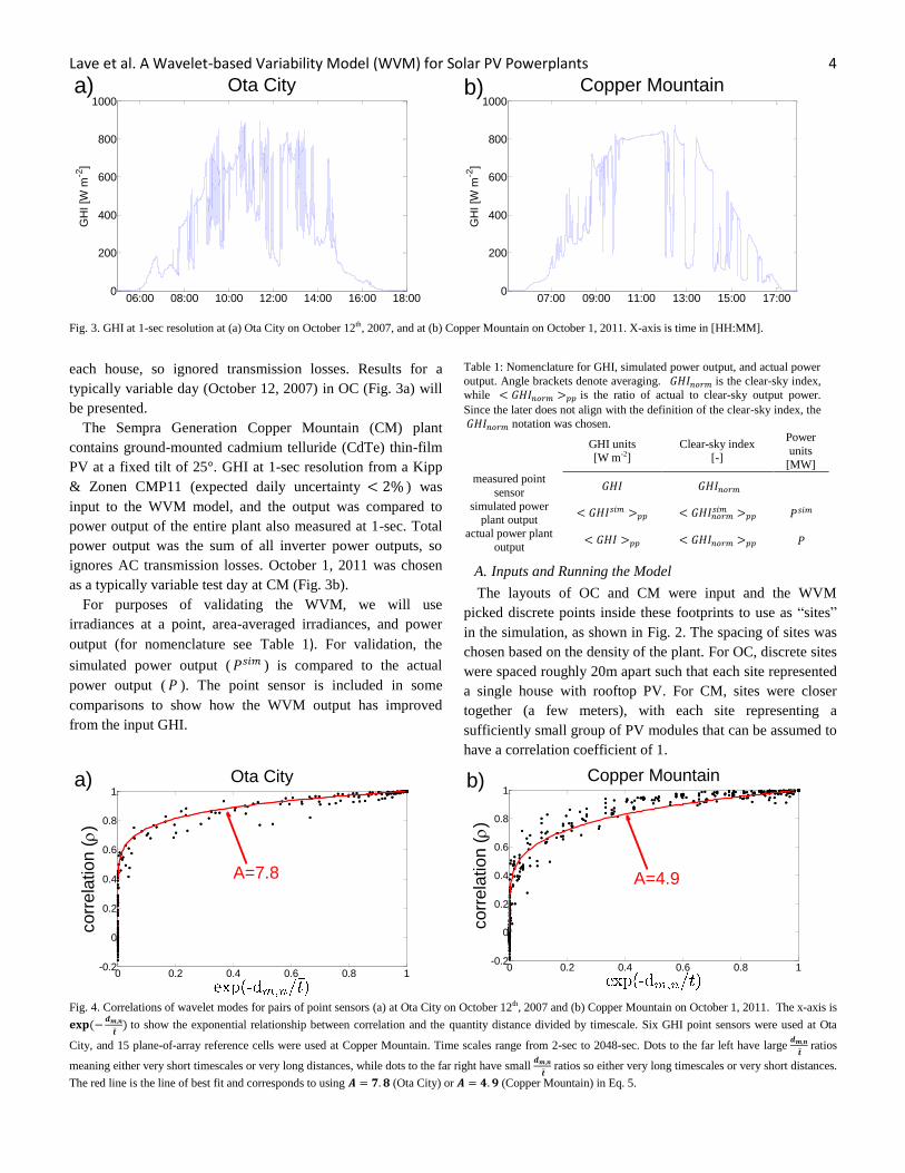
each house, so ignored transmission losses. Results for a

typically variable day (October 12, 2007) in OC (Fig. 3a) will

be presented.

The Sempra Generation Copper Mountain (CM) plant

contains ground-mounted cadmium telluride (CdTe) thin-film

PV at a fixed tilt of 25°. GHI at 1-sec resolution from a Kipp

& Zonen CMP11 (expected daily uncertainty ) was

input to the WVM model, and the output was compared to

power output of the entire plant also measured at 1-sec. Total

power output was the sum of all inverter power outputs, so

ignores AC transmission losses. October 1, 2011 was chosen

as a typically variable test day at CM (Fig. 3b).

For purposes of validating the WVM, we will use

irradiances at a point, area-averaged irradiances, and power

output (for nomenclature see Table 1). For validation, the

simulated power output ( ) is compared to the actual

power output ( ). The point sensor is included in some

comparisons to show how the WVM output has improved

from the input GHI.

Table 1: Nomenclature for GHI, simulated power output, and actual power

output. Angle brackets denote averaging. is the clear-sky index,

while is the ratio of actual to clear-sky output power.

Since the later does not align with the definition of the clear-sky index, the

notation was chosen.

GHI units [W m-2]

Clear-sky index [-]

Power

units

[MW]

measured point

sensor

simulated power plant output

actual power plant

output

A. Inputs and Running the Model

The layouts of OC and CM were input and the WVM

picked discrete points inside these footprints to use as “sites”

in the simulation, as shown in Fig. 2. The spacing of sites was

chosen based on the density of the plant. For OC, discrete sites

were spaced roughly 20m apart such that each site represented

a single house with rooftop PV. For CM, sites were closer

together (a few meters), with each site representing a

sufficiently small group of PV modules that can be assumed to

have a correlation coefficient of 1.

Fig. 3. GHI at 1-sec resolution at (a) Ota City on October 12th, 2007, and at (b) Copper Mountain on October 1, 2011. X-axis is time in [HH:MM].

Fig. 4. Correlations of wavelet modes for pairs of point sensors (a) at Ota City on October 12th, 2007 and (b) Copper Mountain on October 1, 2011. The x-axis is

(

) to show the exponential relationship between correlation and the quantity distance divided by timescale. Six GHI point sensors were used at Ota

City, and 15 plane-of-array reference cells were used at Copper Mountain. Time scales range from 2-sec to 2048-sec. Dots to the far left have large

ratios

meaning either very short timescales or very long distances, while dots to the far right have small

ratios so either very long timescales or very short distances.

The red line is the line of best fit and corresponds to using (Ota City) or (Copper Mountain) in Eq. 5.

06:00 08:00 10:00 12:00 14:00 16:00 18:000

200

400

600

800

1000

GH

I [W

m-2

]Ota Citya)

07:00 09:00 11:00 13:00 15:00 17:000

200

400

600

800

1000

Copper Mountain

GH

I [W

m-2

]

b)

0 0.2 0.4 0.6 0.8 1-0.2

0

0.2

0.4

0.6

0.8

1

corr

ela

tio

n ()

Ota City

a)

A=7.8

0 0.2 0.4 0.6 0.8 1-0.2

0

0.2

0.4

0.6

0.8

1

corr

ela

tion ()

Copper Mountainb)

A=4.9


Also input to the WVM were the GHI measurement vectors,

as well as latitude, longitude, and UTC offset (for creating the

clear-sky model, ). The test day at OC contains large

cloud-induced irradiance fluctuations throughout the day. The

test day at CM has some large irradiance fluctuations as well

as a few clear periods (e.g., 10:00-12:00). Thus, the WVM

model will be tested at two different sites and types of daily

cloud conditions (highly variable and partly variable).

For OC on the test day, , as found from 6 GHI point

sensors. Similarly, 15 plane-of-array reference cells at CM

were used to determine on October 1 (Fig. 4). The

small scatter of correlation points (black dots) around the best-

fit curve, most noticeable at CM, is likely due to small

anisotropic effects (i.e., pairs of sensors arranged in a certain

direction may have higher correlation for all timescales).

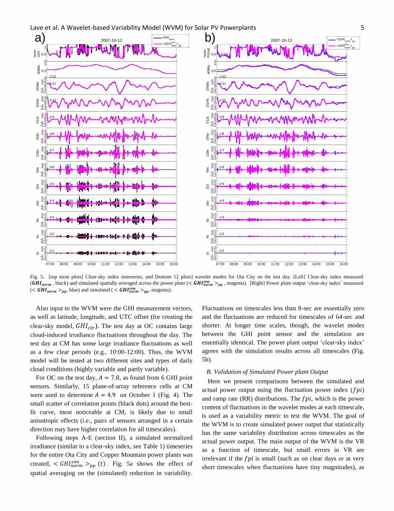
Following steps A-E (section II), a simulated normalized

irradiance (similar to a clear-sky index, see Table 1) timeseries

for the entire Ota City and Copper Mountain power plants was

created, ( ) . Fig. 5a shows the effect of

spatial averaging on the (simulated) reduction in variability.

Fluctuations on timescales less than 8-sec are essentially zero

and the fluctuations are reduced for timescales of 64-sec and

shorter. At longer time scales, though, the wavelet modes

between the GHI point sensor and the simulation are

essentially identical. The power plant output ‘clear-sky index’

agrees with the simulation results across all timescales (Fig.

5b).

B. Validation of Simulated Power plant Output

Here we present comparisons between the simulated and

actual power output using the fluctuation power index ( )

and ramp rate (RR) distributions. The , which is the power

content of fluctuations in the wavelet modes at each timescale,

is used as a variability metric to test the WVM. The goal of

the WVM is to create simulated power output that statistically

has the same variability distribution across timescales as the

actual power output. The main output of the WVM is the VR

as a function of timescale, but small errors in VR are

irrelevant if the is small (such as on clear days or at very

short timescales when fluctuations have tiny magnitudes), as

Fig. 5. [top most plots] Clear-sky index timeseries, and [bottom 12 plots] wavelet modes for Ota City on the test day. [Left] Clear-sky index measured

( , black) and simulated spatially averaged across the power plant ( , magenta). [Right] Power plant output ‘clear-sky index’ measured

( , blue) and simulated ( , magenta).

07:00 08:00 09:00 10:00 11:00 12:00 13:00 14:00 15:00 16:00

-0.2-0.1

00.10.2

2s

j=1

-0.2-0.1

00.10.2

4s

j=2

-0.2-0.1

00.10.2

8s

j=3

-0.2-0.1

00.10.2

16s j=4

-0.2-0.1

00.10.2

32s j=5

-0.2-0.1

00.10.2

64s j=6

-0.2-0.1

00.10.2

128s j=7

-0.2-0.1

00.10.2

256s j=8

-0.2-0.1

00.10.2

512s j=9

-0.2-0.1

00.10.2

1024s j=10

-0.2-0.1

00.10.2

2048s j=11

0

0.5

1

4096s

j=12

0

0.5

1

2007-10-12

norm

.G

HI

GHInorm

<GHIsim

norm>

pp

a)

07:00 08:00 09:00 10:00 11:00 12:00 13:00 14:00 15:00 16:00

-0.2-0.1

00.10.2

2s

j=1

-0.2-0.1

00.10.2

4s

j=2

-0.2-0.1

00.10.2

8s

j=3

-0.2-0.1

00.10.2

16s j=4

-0.2-0.1

00.10.2

32s j=5

-0.2-0.1

00.10.2

64s j=6

-0.2-0.1

00.10.2

128s j=7

-0.2-0.1

00.10.2

256s j=8

-0.2-0.1

00.10.2

512s j=9

-0.2-0.1

00.10.2

1024s j=10

-0.2-0.1

00.10.2

2048s j=11

0

0.5

1

4096s

j=12

0

0.5

1

2007-10-12

norm

.P

/GH

I

<GHInorm

>pp

<GHIsim

norm>

pp

b)


errors will also be very small. However, when the is large

(such as on cloudy days or at long timescales), errors in VR

can lead to significant errors in . Additionally, and

total power output can be slightly offset in time based on the

direction of cloud movement and the location of the GHI

sensor versus the centroid of the power plant. Since the

describes the variability content (and total variance) rather

than the time of occurrence, it allows measuring the accuracy

of the WVM independent of these geographic limitations.

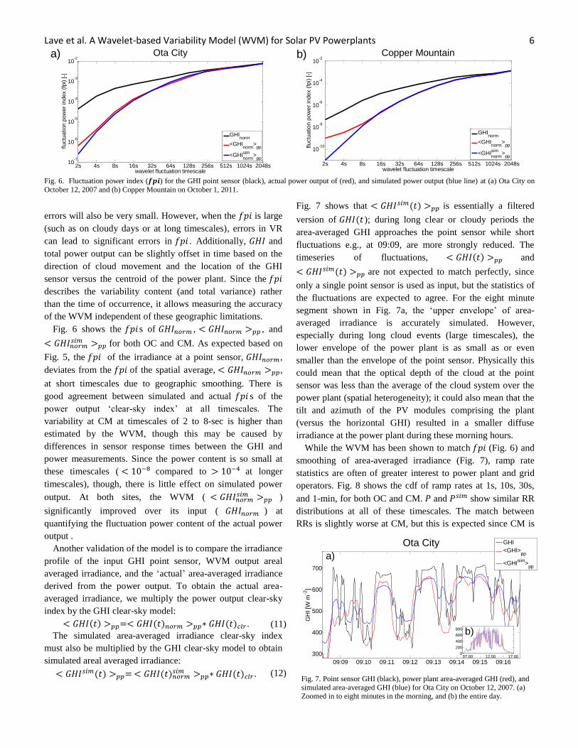
Fig. 6 shows the s of , , and

for both OC and CM. As expected based on

Fig. 5, the of the irradiance at a point sensor, ,

deviates from the of the spatial average, ,

at short timescales due to geographic smoothing. There is

good agreement between simulated and actual s of the

power output ‘clear-sky index’ at all timescales. The

variability at CM at timescales of 2 to 8-sec is higher than

estimated by the WVM, though this may be caused by

differences in sensor response times between the GHI and

power measurements. Since the power content is so small at

these timescales ( compared to at longer

timescales), though, there is little effect on simulated power

output. At both sites, the WVM ( )

significantly improved over its input ( ) at

quantifying the fluctuation power content of the actual power

output .

Another validation of the model is to compare the irradiance

profile of the input GHI point sensor, WVM output areal

averaged irradiance, and the ‘actual’ area-averaged irradiance

derived from the power output. To obtain the actual area-

averaged irradiance, we multiply the power output clear-sky

index by the GHI clear-sky model:

( ) ( ) ( ) . (11)

The simulated area-averaged irradiance clear-sky index

must also be multiplied by the GHI clear-sky model to obtain

simulated areal averaged irradiance:

( ) ( ) ( ) . (12)

Fig. 7 shows that ( ) is essentially a filtered

version of ( ); during long clear or cloudy periods the

area-averaged GHI approaches the point sensor while short

fluctuations e.g., at 09:09, are more strongly reduced. The

timeseries of fluctuations, ( ) and

( ) are not expected to match perfectly, since

only a single point sensor is used as input, but the statistics of

the fluctuations are expected to agree. For the eight minute

segment shown in Fig. 7a, the ‘upper envelope’ of area-

averaged irradiance is accurately simulated. However,

especially during long cloud events (large timescales), the

lower envelope of the power plant is as small as or even

smaller than the envelope of the point sensor. Physically this

could mean that the optical depth of the cloud at the point

sensor was less than the average of the cloud system over the

power plant (spatial heterogeneity); it could also mean that the

tilt and azimuth of the PV modules comprising the plant

(versus the horizontal GHI) resulted in a smaller diffuse

irradiance at the power plant during these morning hours.

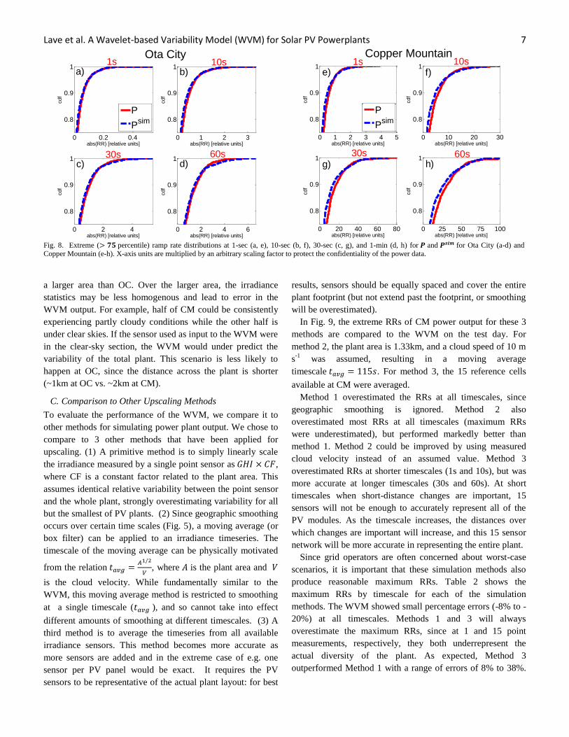
While the WVM has been shown to match (Fig. 6) and

smoothing of area-averaged irradiance (Fig. 7), ramp rate

statistics are often of greater interest to power plant and grid

operators. Fig. 8 shows the cdf of ramp rates at 1s, 10s, 30s,

and 1-min, for both OC and CM. and show similar RR

distributions at all of these timescales. The match between

RRs is slightly worse at CM, but this is expected since CM is

Fig. 6. Fluctuation power index ( ) for the GHI point sensor (black), actual power output of (red), and simulated power output (blue line) at (a) Ota City on

October 12, 2007 and (b) Copper Mountain on October 1, 2011.

Fig. 7. Point sensor GHI (black), power plant area-averaged GHI (red), and

simulated area-averaged GHI (blue) for Ota City on October 12, 2007. (a) Zoomed in to eight minutes in the morning, and (b) the entire day.

2s 4s 8s 16s 32s 64s 128s 256s 512s 1024s 2048s10

-7

10-6

10-5

10-4

10-3

10-2

wavelet fluctuation timescale

fluctu

ation p

ow

er

index (

fpi) [-]

Ota City

GHInorm

<GHInorm

>pp

<GHIsim

norm>

pp

a)

2s 4s 8s 16s 32s 64s 128s 256s 512s 1024s 2048s

10-10

10-8

10-6

10-4

10-2

wavelet fluctuation timescale

fluctu

ation p

ow

er

index (

fpi) [-]

Copper Mountain

GHInorm

<GHInorm

>pp

<GHInorm

sim>

pp

b)

09:09 09:10 09:11 09:12 09:13 09:14 09:15 09:16

300

400

500

600

700

GH

I [W

m-2

]

Ota City

GHI

<GHI>pp

<GHIsim

>pp

07:00 12:00 17:000

200

400

600

800 b)

a)


a larger area than OC. Over the larger area, the irradiance

statistics may be less homogenous and lead to error in the

WVM output. For example, half of CM could be consistently

experiencing partly cloudy conditions while the other half is

under clear skies. If the sensor used as input to the WVM were

in the clear-sky section, the WVM would under predict the

variability of the total plant. This scenario is less likely to

happen at OC, since the distance across the plant is shorter

(~1km at OC vs. ~2km at CM).

C. Comparison to Other Upscaling Methods

To evaluate the performance of the WVM, we compare it to

other methods for simulating power plant output. We chose to

compare to 3 other methods that have been applied for

upscaling. (1) A primitive method is to simply linearly scale

the irradiance measured by a single point sensor as ,

where CF is a constant factor related to the plant area. This

assumes identical relative variability between the point sensor

and the whole plant, strongly overestimating variability for all

but the smallest of PV plants. (2) Since geographic smoothing

occurs over certain time scales (Fig. 5), a moving average (or

box filter) can be applied to an irradiance timeseries. The

timescale of the moving average can be physically motivated

from the relation

, where is the plant area and

is the cloud velocity. While fundamentally similar to the

WVM, this moving average method is restricted to smoothing

at a single timescale ( ), and so cannot take into effect

different amounts of smoothing at different timescales. (3) A

third method is to average the timeseries from all available

irradiance sensors. This method becomes more accurate as

more sensors are added and in the extreme case of e.g. one

sensor per PV panel would be exact. It requires the PV

sensors to be representative of the actual plant layout: for best

results, sensors should be equally spaced and cover the entire

plant footprint (but not extend past the footprint, or smoothing

will be overestimated).

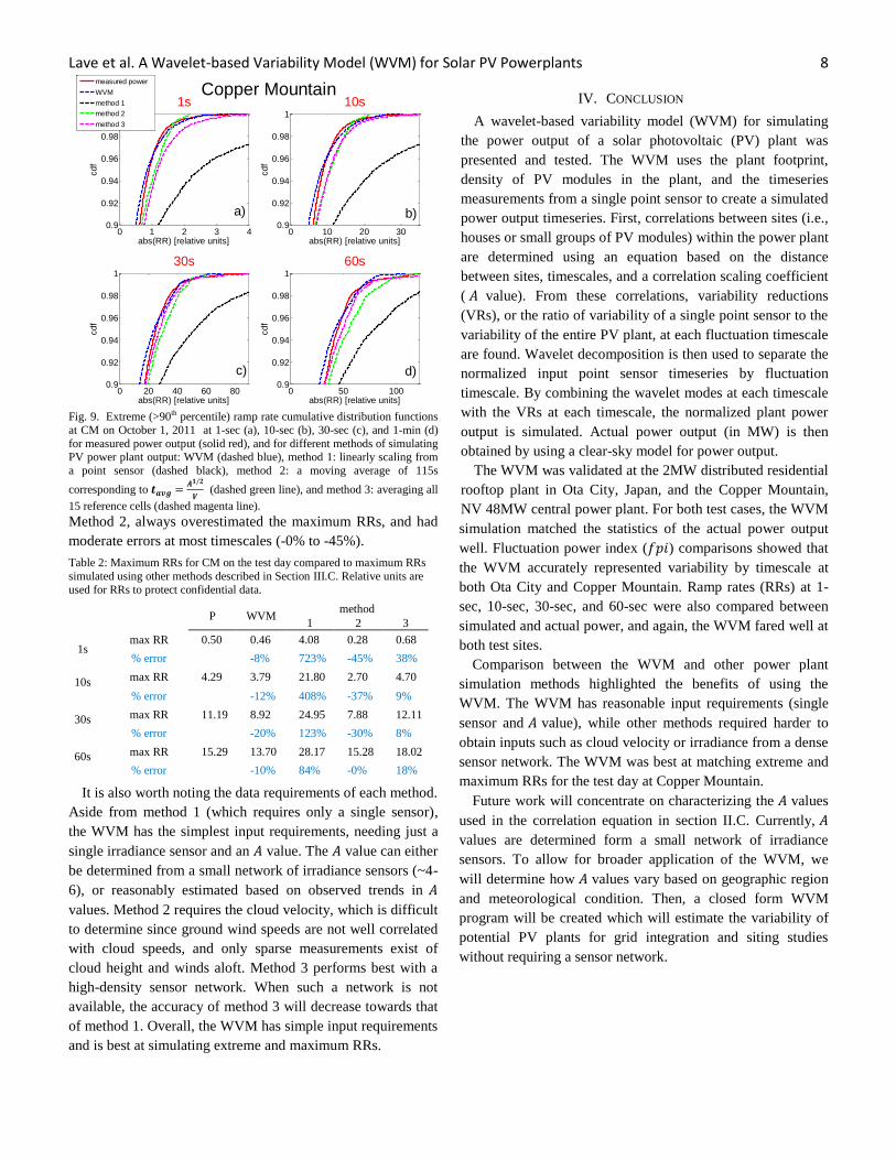
In Fig. 9, the extreme RRs of CM power output for these 3

methods are compared to the WVM on the test day. For

method 2, the plant area is 1.33km, and a cloud speed of 10 m

s-1

was assumed, resulting in a moving average

timescale . For method 3, the 15 reference cells

available at CM were averaged.

Method 1 overestimated the RRs at all timescales, since

geographic smoothing is ignored. Method 2 also

overestimated most RRs at all timescales (maximum RRs

were underestimated), but performed markedly better than

method 1. Method 2 could be improved by using measured

cloud velocity instead of an assumed value. Method 3

overestimated RRs at shorter timescales (1s and 10s), but was

more accurate at longer timescales (30s and 60s). At short

timescales when short-distance changes are important, 15

sensors will not be enough to accurately represent all of the

PV modules. As the timescale increases, the distances over

which changes are important will increase, and this 15 sensor

network will be more accurate in representing the entire plant.

Since grid operators are often concerned about worst-case

scenarios, it is important that these simulation methods also

produce reasonable maximum RRs. Table 2 shows the

maximum RRs by timescale for each of the simulation

methods. The WVM showed small percentage errors (-8% to -

20%) at all timescales. Methods 1 and 3 will always

overestimate the maximum RRs, since at 1 and 15 point

measurements, respectively, they both underrepresent the

actual diversity of the plant. As expected, Method 3

outperformed Method 1 with a range of errors of 8% to 38%.

Fig. 8. Extreme ( percentile) ramp rate distributions at 1-sec (a, e), 10-sec (b, f), 30-sec (c, g), and 1-min (d, h) for and for Ota City (a-d) and Copper Mountain (e-h). X-axis units are multiplied by an arbitrary scaling factor to protect the confidentiality of the power data.

0 0.2 0.4

0.8

0.9

1

abs(RR) [relative units]

cdf

1s

P

Psim

0 1 2 3

0.8

0.9

110s


cdf

0 2 4

0.8

0.9

130s


cdf

0 2 4 6

0.8

0.9

160s


cdf

a) b)

c) d)

Ota City

0 1 2 3 4 5

0.8

0.9

1


cdf

1s

0 10 20 30

0.8

0.9

110s


cdf

0 20 40 60 80

0.8

0.9

130s


cdf

0 25 50 75 100

0.8

0.9

160s


cdf

P

Psim

e)

g) h)

f)

Copper Mountain


Method 2, always overestimated the maximum RRs, and had

moderate errors at most timescales (-0% to -45%).

Table 2: Maximum RRs for CM on the test day compared to maximum RRs

simulated using other methods described in Section III.C. Relative units are

used for RRs to protect confidential data.

P WVM method

1 2 3

1s max RR 0.50 0.46 4.08 0.28 0.68

% error -8% 723% -45% 38%

10s max RR 4.29 3.79 21.80 2.70 4.70

% error -12% 408% -37% 9%

30s max RR 11.19 8.92 24.95 7.88 12.11

% error -20% 123% -30% 8%

60s max RR 15.29 13.70 28.17 15.28 18.02

% error -10% 84% -0% 18%

It is also worth noting the data requirements of each method.

Aside from method 1 (which requires only a single sensor),

the WVM has the simplest input requirements, needing just a

single irradiance sensor and an value. The value can either

be determined from a small network of irradiance sensors (~4-

6), or reasonably estimated based on observed trends in

values. Method 2 requires the cloud velocity, which is difficult

to determine since ground wind speeds are not well correlated

with cloud speeds, and only sparse measurements exist of

cloud height and winds aloft. Method 3 performs best with a

high-density sensor network. When such a network is not

available, the accuracy of method 3 will decrease towards that

of method 1. Overall, the WVM has simple input requirements

and is best at simulating extreme and maximum RRs.

IV. CONCLUSION

A wavelet-based variability model (WVM) for simulating

the power output of a solar photovoltaic (PV) plant was

presented and tested. The WVM uses the plant footprint,

density of PV modules in the plant, and the timeseries

measurements from a single point sensor to create a simulated

power output timeseries. First, correlations between sites (i.e.,

houses or small groups of PV modules) within the power plant

are determined using an equation based on the distance

between sites, timescales, and a correlation scaling coefficient

( value). From these correlations, variability reductions

(VRs), or the ratio of variability of a single point sensor to the

variability of the entire PV plant, at each fluctuation timescale

are found. Wavelet decomposition is then used to separate the

normalized input point sensor timeseries by fluctuation

timescale. By combining the wavelet modes at each timescale

with the VRs at each timescale, the normalized plant power

output is simulated. Actual power output (in MW) is then

obtained by using a clear-sky model for power output.

The WVM was validated at the 2MW distributed residential

rooftop plant in Ota City, Japan, and the Copper Mountain,

NV 48MW central power plant. For both test cases, the WVM

simulation matched the statistics of the actual power output

well. Fluctuation power index ( ) comparisons showed that

the WVM accurately represented variability by timescale at

both Ota City and Copper Mountain. Ramp rates (RRs) at 1-

sec, 10-sec, 30-sec, and 60-sec were also compared between

simulated and actual power, and again, the WVM fared well at

both test sites.

Comparison between the WVM and other power plant

simulation methods highlighted the benefits of using the

WVM. The WVM has reasonable input requirements (single

sensor and value), while other methods required harder to

obtain inputs such as cloud velocity or irradiance from a dense

sensor network. The WVM was best at matching extreme and

maximum RRs for the test day at Copper Mountain.

Future work will concentrate on characterizing the values

used in the correlation equation in section II.C. Currently,

values are determined form a small network of irradiance

sensors. To allow for broader application of the WVM, we

will determine how values vary based on geographic region

and meteorological condition. Then, a closed form WVM

program will be created which will estimate the variability of

potential PV plants for grid integration and siting studies

without requiring a sensor network.

Fig. 9. Extreme (>90th percentile) ramp rate cumulative distribution functions

at CM on October 1, 2011 at 1-sec (a), 10-sec (b), 30-sec (c), and 1-min (d)

for measured power output (solid red), and for different methods of simulating PV power plant output: WVM (dashed blue), method 1: linearly scaling from

a point sensor (dashed black), method 2: a moving average of 115s

corresponding to

(dashed green line), and method 3: averaging all

15 reference cells (dashed magenta line).

0 1 2 3 40.9

0.92

0.94

0.96

0.98

1


cdf

1s

measured power

WVM

method 1

method 2

method 3

0 10 20 300.9

0.92

0.94

0.96

0.98

1

10s


cdf

0 20 40 60 800.9

0.92

0.94

0.96

0.98

1

30s


cdf

0 50 1000.9

0.92

0.94

0.96

0.98

1

60s


cdf

Copper Mountain

a)

c)

b)

d)


ACKNOWLEDGMENT

We appreciate the help of Yusuke Miyamoto and Eichi

Nakashima from Kandenko in Ibaraki, Japan for providing and

supporting the Ota City data, as well as David Jeon, Leslie

Padilla, and Shiva Bahuman from Sempra Energy in San

Diego, California Darryl Lopez from Eldorado Energy, and

Bryan Urquhart from UCSD for providing and supporting the

Copper Mountain data.

REFERENCES

[1] K. Otani, J. Minowa, and K. Kurokawa, "Study on

areal solar irradiance for analyzing areally-totalized

PV systems," Solar Energy Materials and Solar

Cells, vol. 47, pp. 281-288, Oct 1997.

[2] A. E. Curtright and J. Apt, "The character of power

output from utility-scale photovoltaic systems,"

Progress in Photovoltaics, vol. 16, pp. 241-247, May

2008.

[3] M. Lave and J. Kleissl, "Solar variability of four sites

across the state of Colorado," Renewable Energy, vol.

35, pp. 2867-2873, Dec 2010.

[4] E. Wiemken, H. G. Beyer, W. Heydenreich, and K.

Kiefer, "Power characteristics of PV ensembles:

experiences from the combined power production of

100 grid connected PV systems distributed over the

area of Germany," Solar Energy, vol. 70, pp. 513-

518, 2001.

[5] A. Murata, H. Yamaguchi, and K. Otani, "A Method

of Estimating the Output Fluctuation of Many

Photovoltaic Power Generation Systems Dispersed in

a Wide Area," Electrical Engineering in Japan, vol.

166, pp. 9-19, Mar 2009.

[6] A. Mills and R. Wiser, "Implications of Wide-Area

Geographic Diversity for Short-Term Variability of

Solar Power," LBNL Report No. 3884E, 2010.

[7] R. Perez, S. Kivalov, J. Schlemmer, K. Hemker, and

T. Hoff, "Short-term irradiance variability: Station

pair correlation as a function of distance," Submitted

to Solar Energy, 2011.

[8] T. Hoff and R. Perez, "Modeling PV Fleet Output

Variability," Submitted to Solar Energy, 2011.

[9] J. Marcos, L. Marroyo, E. Lorenzo, D. Alvira, and E.

Izco, "From irradiance to output power fluctuations:

the pv plant as a low pass filter," Progress in

Photovoltaics, vol. 19, pp. 505-510, Aug 2011.

[10] P. Ineichen and R. Perez, "A new airmass

independent formulation for the Linke turbidity

coefficient," Solar Energy, vol. 73, pp. 151-157,

2002.

[11] M. Lave, J. Kleissl, and E. Arias-Castro, "High-

frequency irradiance fluctuations and geographic

smoothing," Solar Energy.

[12] J. Page, "The role of solar radiation climatology in

the design of photovoltaic systems," in Practical

handbook of photovoltaics: fundamentals and

applications, T. Markvart and L. Castaner, Eds., ed

Oxford: Elsevier, 2003, pp. 5-66.

[13] J. Boland, B. Ridley, and B. Brown, "Models of

diffuse solar radiation," Renewable Energy, vol. 33,

pp. 575-584, Apr 2008.

[14] C. Hansen, J. Stein, and A. Ellis, "Simulation of One-

Minute Power Output from Utility-Scale Photovoltaic

Generation System," 2011.

[15] D. King, W. Boyson, and J. Kratochvil, "Photovoltaic

Array Performance Model," 2004.

https://www.researchgate.net/publication/255248919_Simulation_of_1-minute_power_output_from_utility-scale_photovoltaic_generation_systems?el=1_x_8&enrichId=rgreq-be79d0ac05fb9d95b86875e3fabee513&enrichSource=Y292ZXJQYWdlOzI1ODIyMDE1MTtBUzo5OTYwOTMzMDMyMzQ1NkAxNDAwNzYwMTI0Mjc0




https://www.researchgate.net/publication/279972199_The_Role_of_Solar_Radiation_Climatology_in_the_Design_of_Photovoltaic_Systems?el=1_x_8&enrichId=rgreq-be79d0ac05fb9d95b86875e3fabee513&enrichSource=Y292ZXJQYWdlOzI1ODIyMDE1MTtBUzo5OTYwOTMzMDMyMzQ1NkAxNDAwNzYwMTI0Mjc0










A wavelet-based variability model (WVM) for solar PV power plants

Documents

Transcript of A wavelet-based variability model (WVM) for solar PV power plants