ELECTRICITY AND MAGNETISM Chapter 1. Electric Fields ...

ELECTRICITY AND MAGNETISM

Chapter 1. Electric Fields

1.1 Introduction

1.2 Triboelectric Effect

1.3 Experiments with Pith Balls

1.4 Experiments with a Gold-leaf Electroscope

1.5 Coulomb’s Law

1.6 Electric Field E

1.6.1 Field of a Point Charge

1.6.2 Spherical Charge Distributions

1.6.3 A Long, Charged Rod

1.6.4 Field on the Axis of and in the Plane of a Charged Ring

1.6.5 Field on the Axis of a Uniformly Charged Disc

1.6.6 Field of a Uniformly Charged Infinite Plane Sheet

1.7 Electric Field D

1.8 Flux

1.9 Gauss’s Theorem

Chapter 2. Electrostatic Potential

2.1 Introduction

2.2 Potential Near Various Charged Bodies

2.2.1 Point Charge


2.2.3 Long Charged Rod

2.2.4 Large Plane Charged Sheet

2.2.5 Potential on the Axis of a Charged Ring

2.2.6 Potential in the Plane of a Charged Ring

2.2.7 Potential on the Axis of a Charged Disc

2.3 Electron-volts

2.4 A Point Charge and an Infinite Conducting Plane

2.5 A Point Charge and a Conducting Sphere

2.6 Two Semicylindrical Electrodes

Chapter 3. Dipole and Quadrupole Moments

3.1 Introduction

3.2 Mathematical Definition of Dipole Moment

3.3 Oscillation of a Dipole in an Electric Field

3.4 Potential Energy of a Dipole in an Electric Field

3.5 Force on a Dipole in an Inhomogeneous Electric Field

3.6 Induced Dipoles and Polarizability

3.7 The Simple Dipole

3.8 Quadrupole Moment

3.9 Potential at a Large Distance from a Charged Body

3.10 A Geophysical Example

Chapter 4. Batteries, Resistors and Ohm’s Law

4.1 Introduction

4.2 Resistance and Ohm’s Law

4.3 Resistance and Temperature

4.4 Resistors in Series

4.5 Conductors in Parallel

4.6 Dissipation of Energy

4.7 Electromotive Force and Internal Resistance

4.8 Power Delivered to an External Resistance

4.9 Potential Divider

4.10 Ammeters and Voltmeters

4.11 Wheatstone Bridge

4.12 Delta-Star Transform

4.13 Kirchhoff’s Rules

4.14 Tortures for the Brain

4.15 Solutions, Answers or Hints to 4.14

4.16 Attenuators

Chapter 5. Capacitors

5.1 Introduction

5.2 Plane Parallel Capacitor

5.3 Coaxial Cylindrical Capacitor

5.4 Concentric Spherical Capacitor

5.5 Capacitors in Parallel

5.6 Capacitors in Series


5.8 Kirchhoff’s Rules

5.9 Problem for a Rainy Day

5.10 Energy Stored in a Capacitor

5.11 Energy Stored in an Electric Field

5.12 Force Between the Plates of a Plane Parallel Plate Capacitor

5.13 Sharing a Charge Between Two Capacitors

5.14 Mixed Dielectrics

5.15 Changing the Distance Between the Plates of a Capacitor

5.16 Inserting a Dielectric into a Capacitor

5.17 Polarization and Susceptibility

5.18 Discharging a Capacitor Through a Resistor

5.19 Charging a Capacitor Through a Resistor

5.20 Real Capacitors

Chapter 6. The Magnetic Effect of an Electric Current

6.1 Introduction

6.2 Definition of the Amp

6.3 Definition of the Magnetic Field

6.4 The Biot-Savart Law

6.5 Magnetic Field Near a Long, Straight, Current-carrying Conductor

6.6 Field on the Axis and in the Plane of a Plane Circular Current-carrying Coil

6.7 Helmholtz Coils

6.8 Field on the Axis of a Long Solenoid

6.9 The Magnetic Field H

6.10 Flux

6.11 Ampère’s Theorem

Chapter 7. Force on a Current in a Magnetic Field

7.1 Introduction

7.2 Force Between Two Current-carrying Wires

7.3 The Permeability of Free Space

7.4 Magnetic Moment

7.5 Magnetic Moment of a Plane, Current-carrying Coil

7.6 Period of Oscillation of a Magnet or a Coil in an External Magnetic Field

7.7 Potential Energy of a Magnet or a Coil in a Magnetic Field

7.8 Moving-coil Ammeter

7.9 Magnetogyric Ratio

Chapter 8. On the Electrodynamics of Moving Bodies

8.1 Introduction

8.2 Charged Particle in an Electric Field

8.3 Charged Particle in a Magnetic Field

8.4 Charged Particle in an Electric and a Magnetic Field

8.5 Motion in a Nonuniform Magnetic Field

8A Appendix. Integration of the Equations

Chapter 9. Magnetic Potential

9.1 Introduction

9.2 The Magnetic Vector Potential

9.3 Long, Straight, Current-carrying Conductor

9.4 Long Solenoid

9.5 Divergence

Chapter 10. Electromagnetic Induction

10.1 Introduction

10.2 Electromagnetic Induction and the Lorentz Force

10.3 Lenz's Law

10.4 Ballistic Galvanometer and the Measurement of Magnetic Field

10.5 AC Generator

10.6 AC Power

10.7 Linear Motors and Generators

10.8 Rotary Motors

10.9 The Transformer

10.10 Mutual Inductance

10.11 Self Inductance

10.12 Growth of Current in a Circuit Containing Inductance

10.13 Discharge of a Capacitor through an Inductance

10.14 Discharge of a Capacitor through an Inductance and a Resistance

10.15 Energy Stored in an Inductance

10.16 Energy Stored in a Magnetic Field

Chapter 11. Dimensions

Chapter 12. Properties of Magnetic Materials

12.1 Introduction

12.2 Magnetic Circuits and Ohm’s Law

12.3 Magnetization and Susceptibility

12.4 Diamagnetism

12.5 Paramagnetism

12.6 Ferromagnetism

12.7 Antiferromagnetism

12.8 Ferrimagnetism

Chapter 13. Alternating Current

13.1 Alternating current in an inductance

13.2 Alternating Voltage across a Capacitor

13.3 Complex Numbers

13.4 Resistance and Inductance in Series

13.5 Resistance and Capacitance in Series

13.6 Admittance

13.7 The RLC Series Acceptor Circuit

13.8 The RLC Parallel Rejector Circuit

13.9 AC Bridges

13.9.1 The Owen Bridge

13.9.2 The Schering Bridge

13.9.3 The Wien Bridge

13.10 The Transformer

Chapter 14. Laplace Transforms

14.1 Introduction

14.2 Table of Laplace Transforms

14.3 The First Integration Theorem

14.4 The Second Integration Theorem (Dividing a Function by t)

14.5 Shifting Theorem

14.6 A Function Times tn

14.7 Differentiation Theorem

14.8 A First Order Differential Equation

14.9 A Second Order Differential Equation

14.10 Generalized Impedance

14.11 RLC Series Transient

14.12 Another Example

Chapter 15. Maxwell’s Equations

15.1 Introduction

15.2 Maxwell's First Equation

15.3 Poisson's and Laplace's Equations

15.4 Maxwell's Second Equation

15.5 Maxwell's Third Equation

15.6 The Magnetic Equivalent of Poisson's Equation

15.7 Maxwell's Fourth Equation

15.8 Summary of Maxwell's and Poisson's Equations

15.9 Electromagnetic Waves

15.10 Gauge Transformations

15.11 Maxwell’s Equations in Potential Form

15.12 Retarded Potential

Chapter 16. CGS Electricity and Magnetism

16.1 Introduction

16.2 The CGS Electrostatic System

16.3 The CGS Electromagnetic System

16.4 The Gaussian Mixed System

16.5 Dimensions

Chapter 17. Magnetic Dipole Moment

17.1 Introduction

17.2 The SI Definition of Magnetic Moment

17.3 The Magnetic Field on the Equator of a Magnet

17.4 CGS Magnetic Moment, and Lip Service to SI

17.5 Possible Alternative Definitions of Magnetic Moment

17.6 Thirteen Questions

17.7 Additional Remarks

17.8 Conclusion

Chapter 18. Electrochemistry

1

CHAPTER 1

ELECTRIC FIELDS

1.1 Introduction

This is the first in a series of chapters on electricity and magnetism. Much of it will be

aimed at an introductory level suitable for first or second year students, or perhaps some

parts may also be useful at high school level. Occasionally, as I feel inclined, I shall go a

little bit further than an introductory level, though the text will not be enough for anyone

pursuing electricity and magnetism in a third or fourth year honours class. On the other

hand, students embarking on such advanced classes will be well advised to know and

understand the contents of these more elementary notes before they begin.

The subject of electromagnetism is an amalgamation of what were originally studies of

three apparently entirely unrelated phenomena, namely electrostatic phenomena of the

type demonstrated with pieces of amber, pith balls, and ancient devices such as Leyden

jars and Wimshurst machines; magnetism, and the phenomena associated with

lodestones, compass needles and Earth’s magnetic field; and current electricity – the sort

of electricity generated by chemical cells such as Daniel and Leclanché cells. These must

have seemed at one time to be entirely different phenomena. It wasn’t until 1820 that

Oersted discovered (during the course of a university lecture, so the story goes) that an

electric current is surrounded by a magnetic field, which could deflect a compass needle.

The several phenomena relating the apparently separate phenomena were discovered

during the nineteenth century by scientists whose names are immortalized in many of the

units used in electromagnetism – Ampère, Ohm, Henry, and, especially, Faraday. The

basic phenomena and the connections between the three disciplines were ultimately

described by Maxwell towards the end of the nineteenth century in four famous

equations. This is not a history book, and I am not qualified to write one, but I strongly

commend to anyone interested in the history of physics to learn about the history of the

growth of our understanding of electromagnetic phenomena, from Gilbert’s description

of terrestrial magnetism in the reign of Queen Elizabeth I, through Oersted’s discovery

mentioned above, up to the culmination of Maxwell’s equations.

This set of notes will be concerned primarily with a description of electricity and

magnetism as natural phenomena, and it will be treated from the point of view of a

“pure” scientist. It will not deal with the countless electrical devices that we use in our

everyday life – how they work, how they are designed and how they are constructed.

These matters are for electrical and electronics engineers. So, you might ask, if your

primary interest in electricity is to understand how machines, instruments and electrical

equipment work, is there any point in studying electricity from the very “academic” and

abstract approach that will be used in these notes, completely divorced as they appear to

be from the world of practical reality? The answer is that electrical engineers more than

anybody must understand the basic scientific principles before they even begin to apply

them to the design of practical appliances. So – do not even think of electrical

engineering until you have a thorough understanding of the basic scientific principles of

the subject.

2

This chapter deals with the basic phenomena, definitions and equations concerning

electric fields.

1.2 Triboelectric Effect

In an introductory course, the basic phenomena of electrostatics are often demonstrated

with “pith balls” and with a “gold-leaf electroscope”. A pith ball used to be a small, light

wad of pith extracted from the twig of an elder bush, suspended by a silk thread. Today,

it is more likely to be either a ping-pong ball, or a ball of styrofoam, suspended by a

nylon thread – but, for want of a better word, I’ll still call it a pith ball. I’ll describe the

gold-leaf electroscope a little later.

It was long ago noticed that if a sample of amber (fossilized pine sap) is rubbed with

cloth, the amber became endowed with certain apparently wonderful properties. For

example, the amber would be able to attract small particles of fluff to itself. The effect is

called the triboelectric effect. [Greek τρίβος (rubbing) + ήλεκτρον (amber)] The amber,

after having been rubbed with cloth, is said to bear an electric charge, and space in the

vicinity of the charged amber within which the amber can exert its attractive properties is

called an electric field.

Amber is by no means the best material to demonstrate triboelectricity. Modern plastics

(such as a comb rubbed through the hair) become easily charged with electricity

(provided that the plastic, the cloth or the hair, and the atmosphere, are dry). Glass

rubbed with silk also carries an electric charge – but, as we shall see in the next section,

the charge on glass rubbed with silk seems to be not quite the same as the charge on

plastic rubbed with cloth.

1.3 Experiments with Pith Balls

A pith ball hangs vertically by a thread. A plastic rod is charged by rubbing with cloth.

The charged rod is brought close to the pith ball without touching it. It is observed that

the charged rod weakly attracts the pith ball. This may be surprising – and you are right

to be surprised, for the pith ball carries no charge. For the time being we are going to put

this observation to the back of our minds, and we shall defer an explanation to a later

chapter. Until then it will remain a small but insistent little puzzle.

We now touch the pith ball with the charged plastic rod. Immediately, some of the

magical property (i.e. some of the electric charge) of the rod is transferred to the pith ball,

and we observe that thereafter the ball is strongly repelled from the rod. We conclude

that two electric charges repel each other. Let us refer to the pith ball that we have just

charged as Ball A.

Now let’s do exactly the same experiment with the glass rod that has been rubbed with

silk. We bring the charged glass rod close to an uncharged Ball B. It initially attracts it

3

weakly – but we’ll have to wait until Chapter 2 for an explanation of this unexpected

behaviour. However, as soon as we touch Ball B with the glass rod, some charge is

transferred to the ball, and the rod thereafter repels it. So far, no obvious difference

between the properties of the plastic and glass rods.

But... now bring the glass rod close to Ball A, and we see that Ball A is strongly

attracted. And if we bring the plastic rod close to Ball B, it, too, is strongly attracted.

Furthermore, Balls A and B attract each other.

We conclude that there are two kinds of electric charge, with exactly opposite properties.

We arbitrarily call the kind of charge on the glass rod and on Ball B positive and the

charge on the plastic rod and Ball A negative. We observe, then, that like charges (i.e.

those of the same sign) repel each other, and unlike charges (i.e. those of opposite sign)

attract each other.

1.4 Experiments with a Gold-leaf Electroscope

A gold-leaf electroscope has a vertical rod R attached to a flat metal plate P. Gold is a

malleable metal which can be hammered into extremely thin and light sheets. A light

gold leaf G is attached to the lower end of the rod.

If the electroscope is positively charged by touching the plate with a positively charged

glass rod, G will be repelled from R, because both now carry a positive charge.

You can now experiment as follows. Bring a positively charged glass rod close to P.

The leaf G diverges further from R. We now know that this is because the metal (of

which P, R and G are all composed) contains electrons, which are negatively charged

P

R

G

FIGURE I.1

4

particles that can move about more or less freely inside the metal. The approach of the

positively charged glass rod to P attracts electrons towards P, thus increasing the excess

positive charge on G and the bottom end of R. G therefore moves away from R.

If on the other hand you were to approach P with a negatively charged plastic rod,

electrons would be repelled from P down towards the bottom of the rod, thus reducing the

excess positive charge there. G therefore approaches R.

Now try another experiment. Start with the electroscope uncharged, with the gold leaf

hanging limply down. (This can be achieved by touching P briefly with your finger.)

Approach P with a negatively charged plastic rod, but don’t touch. The gold leaf

diverges from R. Now, briefly touch P with a finger of your free hand. Negatively

charged electrons run down through your body to ground (or earth). Don’t worry – you

won’t feel a thing. The gold leaf collapses, though by this time the electroscope bears a

positive charge, because it has lost some electrons through your body. Now remove the

plastic rod. The gold leaf diverges again. By means of the negatively charged plastic rod

and some deft work with your finger, you have induced a positive charge on the

electroscope. You can verify this by approaching P alternately with a plastic (negative)

or glass (positive) rod, and watch what happens to the gold leaf.

1.5 Coulomb’s Law

If you are interested in the history of physics, it is well worth reading about the important

experiments of Charles Coulomb in 1785. In these experiments he had a small fixed

metal sphere which he could charge with electricity, and a second metal sphere attached

to a vane suspended from a fine torsion thread. The two spheres were charged and,

because of the repulsive force between them, the vane twisted round at the end of the

torsion thread. By this means he was able to measure precisely the small forces between

the charges, and to determine how the force varied with the amount of charge and the

distance between them.

From these experiments resulted what is now known as Coulomb’s Law. Two electric

charges of like sign repel each other with a force that is proportional to the product of

their charges and inversely proportional to the square of the distance between them:

.2

21

r

QQF ∝ 1.5.1

Here Q1 and Q2 are the two charges and r is the distance between them.

We could in principle use any symbol we like for the constant of proportionality, but in

standard SI (Système International) practice, the constant of proportionality is written as

,4

1

πε so that Coulomb’s Law takes the form

5

.4

12

21

r

QQF

πε= 1.5.2

Here ε is called the permittivity of the medium in which the charges are situated, and it

varies from medium to medium. The permittivity of a vacuum (or of “free space”) is

given the symbol ε0. Media other than a vacuum have permittivities a little greater than

ε0. The permittivity of air is very little different from that of free space, and, unless

specified otherwise, I shall assume that all experiments described in this chapter are done

either in free space or in air, so that I shall write Coulomb’s Law as

.4

12

21

0 r

QQF

πε= 1.5.3

You may wonder – why the factor 4π? In fact it is very convenient to define the permittivity in this

manner, with 4π in the denominator, because, as we shall see, it will ensure that all formulas that describe

situations of spherical symmetry will include a 4π, formulas that describe situations of cylindrical

symmetry will include 2π, and no π will appear in formulas involving uniform fields. Some writers

(particularly those who favour cgs units) prefer to incorporate the 4π into the definition of the permittivity,

so that Coulomb’s law appears in the form ,)/( 2

021 rQQF ε= though it is standard SI practice to

define the permittivity as in equation 1.5.3. The permittivity defined by equation 1.5.3 is known as the

“rationalized” definition of the permittivity, and it results in much simpler formulas throughout

electromagnetic theory than the “unrationalized” definition.

The SI unit of charge is the coulomb, C. Unfortunately at this stage I cannot give you an

exact definition of the coulomb, although, if a current of 1 amp flows for a second, the

amount of electric charge that has flowed is 1 coulomb. This may at first seem to be very

clear, until you reflect that we have not yet defined what is meant by an amp, and that,

I’m afraid, will have to come in a much later chapter.

Until then, I can give you some small indications. For example, the charge on an electron

is about −1.6022 × 10−19

C, and the charge on a proton is about +1.6022 × 10−19

C. That

is to say, a collection of 6.24 × 1018

protons, if you could somehow bundle them all

together and stop them from flying apart, amounts to a charge of 1 C. A mole of protons

(i.e. 6.022 × 1023

protons) which would have a mass of about one gram, would have a

charge of 9.65 × 104 C, which is also called a faraday (which is not at all the same thing

as a farad).

[The current definition of the coulomb and the amp, which will be given in Chapter 6, requires some

knowledge of electromagnetism. However, it is likely that, in 2015, the coulomb will be redefined in such

a manner that the magnitude of the charge on a single electron is exactly 1.60217 % 10−19 C.]

The charges involved in our experiments with pith balls, glass rods and gold-leaf

electroscopes are very small in terms of coulombs, and are typically of the order of

nanocoulombs.

The permittivity of free space has the approximate value

6

.mNC108542.8 21212

0

−−−×=ε

Later on, when we know what is meant by a “farad”, we shall use the units F m−1

to

describe permittivity – but that will have to wait until section 5.2.

You may well ask how the permittivity of free space is measured. A brief answer might

be “by carrying out experiments similar to those of Coulomb”. However – and this is

rather a long story, which I shall not describe here – it turns out that since we today

define the metre by defining the speed of light, c, to be exactly 2.997 925 58 × 108 m s

−1,

the permittivity of free space has a defined value, given, in SI units, by

.104

2

7

0c

=πε

It is therefore not necessary to measure ε0 any more than it is necessary to measure c.

But that, as I say, is a long story.

[But if, as is likely, the new definition of the coulomb, referred to on the previous page, becomes official in

2015, ε0 will no longer have an exact defined value, but its measured value will be approximately 8.8542 % 10

−12 C

2 N

−1 m

−2. Many teaching laboratories run an undergraduate experiment in which students measure

the charge on a capacitor of known physical dimensions and a measured potential difference between the

plates, and this enables the measured value of ε0 to be calculated.]

From the point of view of dimensional analysis, electric charge cannot be expressed in

terms of M, L and T, but it has a dimension, Q, of its own. (This assertion is challenged

by some, but this is not the place to discuss the reasons. I may add a chapter, eventually,

discussing this point much later on.) We say that the dimensions of electric charge are Q.

Exercise: Show that the dimensions of permittivity are

[ε0] = M−1

L−3

T2

Q2.

I shall strongly advise the reader to work out and make a note of the dimensions of every

new electric or magnetic quantity as it is introduced.

Exercise: Calculate the magnitude of the force between two point charges of 1 C each

(that’s an enormous charge!) 1 m apart in vacuo.

The answer, of course, is 1/(4πε0), and that, as we have just seen, is c2/10

7 = 9 × 10

9 N,

which is equal to the weight of a mass of 9.2 × 105 tonnes or nearly a million tonnes.

Exercise: Calculate the ratio of the electrostatic to the gravitational force between two

electrons. The numbers you will need are: Q = 1.60 × 10−19

C, m = 9.11 × 10−31

kg, ε0

= 8.85 × 10−12

N m2 C

−2 , G = 6.67 × 10

−11 N m

2 kg

−2 .

7

The answer, which is independent of their distance apart, since both forces fall off

inversely as the square of the distance, is ),4/( 2

0

2GmQ πε (and you should verify that this

is dimensionless), and this comes to 4.2 × 1042

. This is the basis of the oft-heard

statement that electrical forces are 1042

times as strong as gravitational forces – but such a

statement out of context is rather meaningless. For example, the gravitational force

between Earth and Moon is much more than the electrostatic force (if any) between them,

and cosmologists could make a good case for saying that the strongest forces in the

Universe are gravitational.

The ratio of the permittivity of an insulating substance to the permittivity of free space is

its relative permittivity, also called its dielectric constant. The dielectric constants of

many commonly-encountered insulating substances are of order “a few”. That is,

somewhere between 2 and 10. Pure water has a dielectric constant of about 80, which is

quite high (but bear in mind that most water is far from pure and is not an insulator.)

Some special substances, known as ferroelectric substances, such as strontium titanate

SrTiO3, have dielectric constants of a few hundred.

1.6 Electric Field E

The region around a charged body within which it can exert its electrostatic influence

may be called an electric field. In principle, it extends to infinity, but in practice it falls

off more or less rapidly with distance. We can define the intensity or strength E of an

electric field as follows. Suppose that we place a small test charge q in an electric field.

This charge will then experience a force. The ratio of the force to the charge is called the

intensity of the electric field, or, more usually, simply the electric field. Thus I have used

the words “electric field” to mean either the region of space around a charged body, or,

quantitatively, to mean its intensity. Usually it is clear from the context which is meant,

but, if you wish, you may elect to use the longer phrase “intensity of the electric field” if

you want to remove all doubt. The field and the force are in the same direction, and the

electric field is a vector quantity, so the definition of the electric field can be written as

F = QE . 1.6.1

The SI units of electric field are newtons per coulomb, or N C−1

. A little later, however,

we shall come across a unit called a volt, and shall learn that an alternative (and more

usual) unit for electric field is volts per metre, or V m−1

. The dimensions are MLT−2

Q−1

.

You may have noticed that I supposed that we place a “small” test charge in the field, and you may have

wondered why it had to be small, and how small. The problem is that, if we place a large charge in an

electric field, this will change the configuration of the electric field and hence frustrate our efforts to

measure it accurately. So – it has to be sufficiently small so as not to change the configuration of the field

that we are trying to measure. How small is that? Well, it will have to mean infinitesimally small. I hope

that is clear! (It is a bit like that pesky particle of negligible mass m that keeps appearing in mechanics

problems!)

8

We now need to calculate the intensity of an electric field in the vicinity of various

shapes and sizes of charged bodes, such as rods, discs, spheres, and so on.

1.6.1 Field of a point charge

It follows from equation 1.5.3 and the definition of electric field intensity that the electric

field at a distance r from a point charge Q is of magnitude

.4 2

0r

QE

πε= 1.6.2

This can be written in vector form:

.4

ˆ4 3

0

2

0

r r

Q

r

Q

πε=

πε= rE 1.6.3

Here r is a unit vector in the radial direction, and r is a vector of length r in the radial

direction.


I shall not here give calculus derivations of the expressions for electric fields resulting

from spherical charge distributions, since they are identical with the derivations for the

gravitational fields of spherical mass distributions in the Classical Mechanics “book” of

these physics notes, provided that you replace mass by charge and G by )4/(1 0πε− . See

Chapter 5, subsections 5.4.8 and 5.4.9 of Celestial Mechanics. Also, we shall see later

that they can be derived more easily from Gauss’s law than by calculus. I shall, however,

give the results here.

At a distance r from the centre of a hollow spherical shell of radius a bearing a charge Q,

the electric field is zero at any point inside the sphere (i.e. for r < a). For a point outside

the sphere (i.e. r > a) the field intensity is

.4 2

0r

QE

πε= 1.6.4

This is the same as if all the charge were concentrated at a point at the centre of the

sphere.

If you have a spherically-symmetric distribution of charge Q contained within a spherical

volume of radius a, this can be considered as a collection of nested hollow spheres. It

follows that at a point outside a spherically-symmetric distribution of charge, the field at

a distance r from the centre is again

9

.4 2

0r

QE

πε= 1.6.5

That is, it is the same as if all the charge were concentrated at the centre. However, at a

point inside the sphere, the charge beyond the distance r from the centre contributes zero

to the electric field; the electric field at a distance r from the centre is therefore just

.4 2

0r

QE

r

πε= 1.6.6

Here Qr is the charge within a radius r. If the charge is uniformly distributed throughout

the sphere, this is related to the total charge by ,

3

Qa

rQ

r

= where Q is the total

charge. Therefore, for a uniform spherical charge distribution the field inside the sphere

is

.4 3

0a

QrE

πε= 1.6.7

That is to say, it increases linearly from centre to the surface, where it reaches a value of

,4 2

0a

Q

πε whereafter it decreases according to equation 1.6.5.

It is not difficult to imagine some electric charge distributed (uniformly or otherwise)

throughout a finite spherical volume, but, because like charges repel each other, it may

not be easy to realize this idealized situation in practice. In particular, if a metal sphere is

charged, since charge can flow freely through a metal, the self-repulsion of charges will

result in all the charge residing on the surface of the sphere, which then behaves as a

hollow spherical charge distribution with zero electric field within.

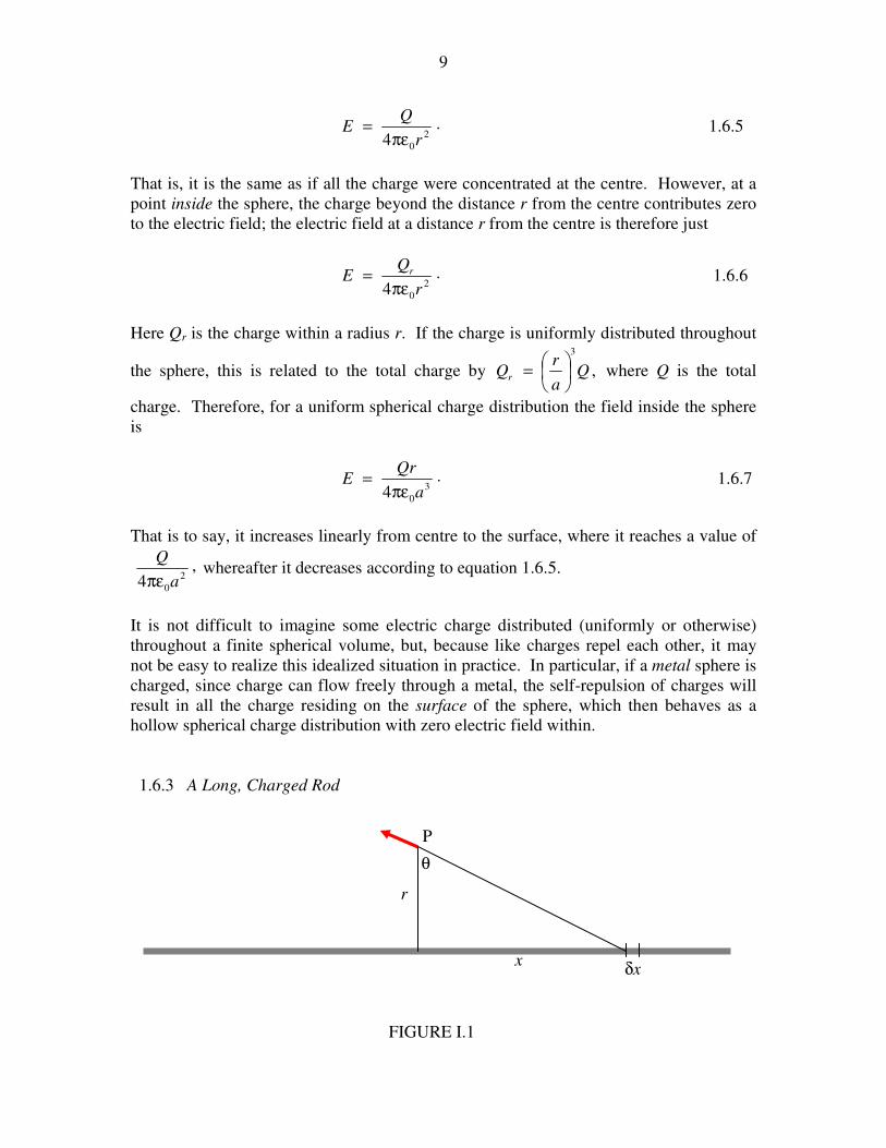
1.6.3 A Long, Charged Rod

r

x δx

θ

FIGURE I.1

P

10

A long rod bears a charge of λ coulombs per metre of its length. What is the strength of

the electric field at a point P at a distance r from the rod?

Consider an element δx of the rod at a distance 2/122 )( xr + from the rod. It bears a

charge λ δx. The contribution to the electric field at P from this element is

22

0

.4

1

xr

x

+

δλ

πεin the direction shown. The radial component of this is

.cos.4

122

0

θ+

δλ

πε xr

x But .secandsec,tan 22222 θ=+δθθ=δθ= rxrrxrx

Therefore the radial component of the field from the element δx is .cos4 0

δθθπε

λ

r To

find the radial component of the field from the entire rod, we integrate along the length of

the rod. If the rod is infinitely long (or if its length is much greater than r), we integrate

from θ = −π/2 to + π/2, or, what amounts to the same thing, from 0 to π/2, and double it.

Thus the radial component of the field is

.2

cos4

2

0

2/

00 rr

Eπε

λ=δθθ

πε

λ= ∫

π

1 6.8

The component of the field parallel to the rod, by considerations of symmetry, is zero, so

equation 1.6.8 gives the total field at a distance r from the rod, and it is directed radially

away from the rod.

Notice that equation 1.6.4 for a spherical charge distribution has 4πr2 in the denominator,

while equation 1.6.8, dealing with a problem of cylindrical symmetry, has 2πr.

11

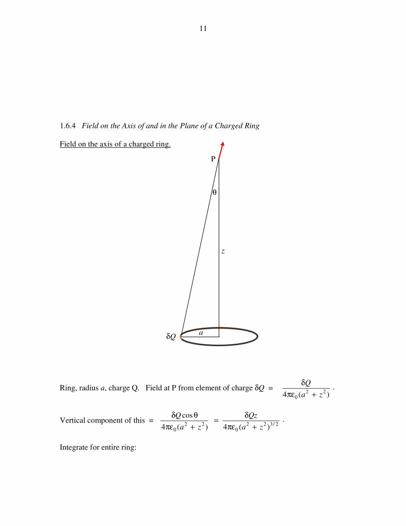
1.6.4 Field on the Axis of and in the Plane of a Charged Ring

Field on the axis of a charged ring.

Ring, radius a, charge Q. Field at P from element of charge δQ = .)(4 22

0 za

Q

+πε

δ

Vertical component of this = .)(4)(4

cos2/322

022

0 za

Qz

za

Q

+πε

δ=

+πε

θδ

Integrate for entire ring:

a

z

δQ

θ

P

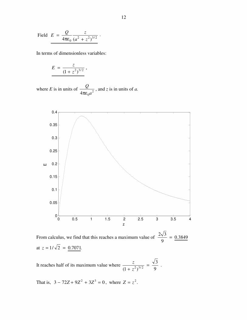
12

Field .)(4 2/322

0 za

zQE

+πε=

In terms of dimensionless variables:

,)1( 2/32

z

zE

+=

where E is in units of 2

04 a

Q

πε, and z is in units of a.

0 0.5 1 1.5 2 2.5 3 3.5 40

0.05

0.1

0.15

0.2

0.25

0.3

0.35

0.4

z

E

From calculus, we find that this reaches a maximum value of 3849.09

32=

at .7071.02/1 ==z

It reaches half of its maximum value where .9

3

)1( 2/32=

+ z

z

That is, 039723 32 =++− ZZZ , where .2zZ =

13

The two positive solution are Z = 0.041889 and 3.596267.

That is, .8964.1and2047.0=z

Field in the plane of a charged ring.

We suppose that we have a ring of radius a bearing a charge Q. We shall try to find the

field at a point in the plane of the ring and at a distance )0( arr <≤ from the centre of

the ring.

Consider an element δθ of the ring at P. The charge on it is π

δθ

2

Q. The field at A due

this element of charge is

,cos

.2.4cos2

1.2

.4

12

022

0 θ−

δθ

ππε=

θ−+π

δθ

πε cba

Q

arra

Q

where 22/1 arb += and ./2 arc = The component of this toward the centre is

θ A

P

a

r

φ

p

14

.cos

cos.2.4 2

0 θ−

δθφ

ππε−

cba

Q

To find the field at A due to the entire ring, we must express φ in terms of θ, r and a, and

integrate with respect to θ from 0 to 2π (or from 0 to π and double it). The necessary

relations are

.2

cos

,cos2

222

222

rp

apr

arrap

−+=φ

θ−+=

The result of the numerical integration is shown below, in which the field is expressed in

units of )4/( 20aQ πε and r is in units of a.

-1 -0.8 -0.6 -0.4 -0.2 0 0.2 0.4 0.6 0.8 1-8

-6

-4

-2

0

2

4

6

8

r

Fie

ld

15

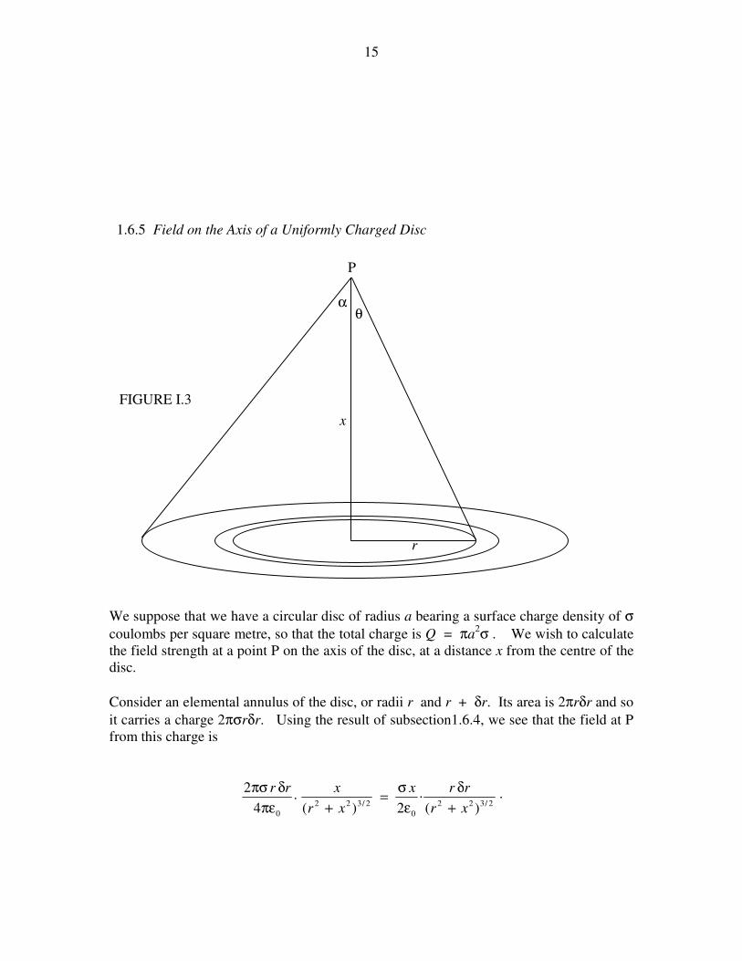
1.6.5 Field on the Axis of a Uniformly Charged Disc

We suppose that we have a circular disc of radius a bearing a surface charge density of σ

coulombs per square metre, so that the total charge is Q = πa2σ . We wish to calculate

the field strength at a point P on the axis of the disc, at a distance x from the centre of the

disc.

Consider an elemental annulus of the disc, or radii r and r + δr. Its area is 2πrδr and so

it carries a charge 2πσrδr. Using the result of subsection1.6.4, we see that the field at P

from this charge is

.)(

.2)(

.4

22/322

0

2/322

0 xr

rrx

xr

xrr

+

δ

ε

σ=

+πε

δπσ

α θ

x

P

r

FIGURE I.3

16

But .sec)(andsec,tan 2/1222 θ=+δθθ=δθ= xxrxrxr Thus the field from

the elemental annulus can be written

.sin2 0

δθθε

σ

The field from the entire disc is found by integrating this from θ = 0 to θ = α to obtain

.)(

12

)cos1(2 2/122

00

+−

ε

σ=α−

ε

σ=

xa

xE 1.6.11

This falls off monotonically from σ/(2ε0) just above the disc to zero at infinity.

1.6.6 Field of a Uniformly Charged Infinite Plane Sheet

All we have to do is to put α = π/2 in equation 1.6.10 to obtain

.2 0ε

σ=E 1.6.12

This is independent of the distance of P from the infinite charged sheet. The electric field

lines are uniform parallel lines extending to infinity.

Summary

Point charge Q: .4 2

0r

QE

πε=

Hollow Spherical Shell: E = zero inside the shell,

2

04 r

QE

πε= outside the shell.

Infinite charged rod: .2 0r

Eπε

λ=

Infinite plane sheet: .2 0ε

σ=E

17

1.7 Electric Field D

We have been assuming that all “experiments” described have been carried out in a

vacuum or (which is almost the same thing) in air. But what if the point charge, the

infinite rod and the infinite charged sheet of section 1.6 are all immersed in some medium

whose permittivity is not ε0, but is instead ε? In that case, the formulas for the field

become

.2

,2

,4 2 ε

σ

πε

λ

πε=

rr

QE

There is an ε in the denominator of each of these expressions. When dealing with media

with a permittivity other than ε0 it is often convenient to describe the electric field by

another vector, D, defined simply by

D = εE 1.7.1

In that case the above formulas for the field become just

.2

,2

,4 2

σ

π

λ

π=

rr

QD

The dimensions of D are Q L−2

, and the SI units are C m−2

.

This may seem to be rather trivial, but it does turn out to be more important than it may

seem at the moment.

Equation 1.7.1 would seem to imply that the electric field vectors E and D are just

vectors in the same direction, differing in magnitude only by the scalar quantity ε. This is

indeed the case in vacuo or in any isotropic medium – but it is more complicated in an

anisotropic medium such as, for example, an orthorhombic crystal. This is a crystal

shaped like a rectangular parallelepiped. If such a crystal is placed in an electric field,

the magnitude of the permittivity depends on whether the field is applied in the x- , the y-

or the z-direction. For a given magnitude of E, the resulting magnitude of D will be

different in these three situations. And, if the field E is not applied parallel to one of the

crystallographic axes, the resulting vector D will not be parallel to E. The permittivity in

equation 1.7.1 is a tensor with nine components, and, when applied to E it changes its

direction as well as its magnitude.

However, we shan’t dwell on that just yet, and, unless specified otherwise, we shall

always assume that we are dealing with a vacuum (in which case D = ε0E) or an isotropic

18

medium (in which case D = εE). In either case the permittivity is a scalar quantity and D

and E are in the same direction.

1.8 Flux

The product of electric field intensity and area is the flux ΦE. Whereas E is an intensive

quantity, ΦE is an extensive quantity. It dimensions are ML3T

−2Q

−1 and its SI units are N

m2 C

−1, although later on, after we have met the unit called the volt, we shall prefer to

express ΦE in V m.

With increasing degrees of sophistication, flux may be defined mathematically as:

ΦE = EA

AE •=θ=Φ cosE EA

Note that E is a vector, but ΦE is a scalar.

∫∫ •=Φ AE dE

We can also define a D-flux by .D ∫∫ •=Φ AD d The dimensions of DΦ are just Q

and the SI units are coulombs (C).

A

E

E θ

A

δA

E

FIGURE I.4

FIGURE I.6

FIGURE I.5

19

An example is in order:

Consider a square of side 2a in the xy-plane as shown. Suppose there is a positive charge

Q at a height a on the z-axis. Calculate the total D-flux, ΦD through the area.

Consider an elemental area dxdy at (x, y , 0). Its distance from Q is ,)( 2/1222yxa ++ so

the magnitude of the D-field there is .1

.4 222

yxa

Q

++π The scalar product of this with

the area is ,cos.1

.4 222

dxdyyxa

Qθ

++π and .

)(cos

2/1222yxa

a

++=θ The surface

integral of D over the whole area is

.)(0 0 2/3222∫ ∫∫∫ ++π

=•a a

yxa

dxdyQadAD 1.8.1

x

y

z

θ

Q •

FIGURE I.7

a

a

2a

D

20

Now all we have to do is the nice and easy integral. Let ,tan22 ψ+= yax and the

inner integral ∫ ++

a

yxa

dx

0 2/3222 )( reduces, after some modest algebra, to

.2)( 2222

yaya

a

++ Thus we now have

.

2)(0 2222

2

∫∫∫++π

=•a

yaya

dyQadAD 1.8.2

With the further substitution ,sec222 ω=+ aya this reduces, after more careful

algebra, to

.6∫∫ =•Q

dAD 1.8.3

Two additional examples of calculating surface integrals may be found in Chapter 5,

section 5.6, of the Celestial Mechanics section of these notes. These deal with

gravitational fields, but they are essentially the same as the electrostatic case; just

substitute Q for m and −1/(4πε) for G.

I urge readers actually to go through the pain and the algebra and the trigonometry of

these three examples in order that they may appreciate all the more, in the next section,

the power of Gauss’s theorem.

1.9 Gauss’s Theorem

A point charge Q is at the centre of a sphere of radius r. Calculate the D-flux through the

sphere. Easy. The magnitude of D at a distance a is Q/(4πr2) and the surface area of the

sphere is 4πr2. Therefore the flux is just Q. Notice that this is independent of r; if you

double r, the area is four times as great, but D is only a quarter of what it was, so the total

flux remains the same. You will probably agree that if the charge is surrounded by a

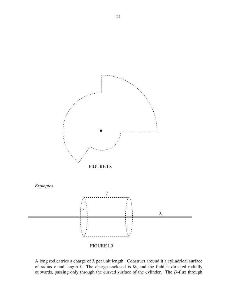
shape such as shown in figure I.8, which is made up of portions of spheres of different

radii, the D-flux through the surface is still just Q. And you can distort the surface as

much as you like, or you may consider any surface to be made up of an infinite number

of infinitesimal spherical caps, and you can put the charge anywhere you like inside the

surface, or indeed you can put as many charges inside as you like – you haven’t changed

the total normal component of the flux, which is still just Q. This is Gauss’s theorem,

which is a consequence of the inverse square nature of Coulomb’s law.

The total normal component of the D-flux through any closed surface is equal to the

charge enclosed by that surface.

21

Examples

A long rod carries a charge of λ per unit length. Construct around it a cylindrical surface

of radius r and length l. The charge enclosed is lλ, and the field is directed radially

outwards, passing only through the curved surface of the cylinder. The D-flux through

•

FIGURE I.8

r

l

FIGURE I.9

λ

22

the cylinder is lλ and the area of the curved surface is 2πrl, so D = lλ/(2πrl) and hence

).2/( rE πελ=

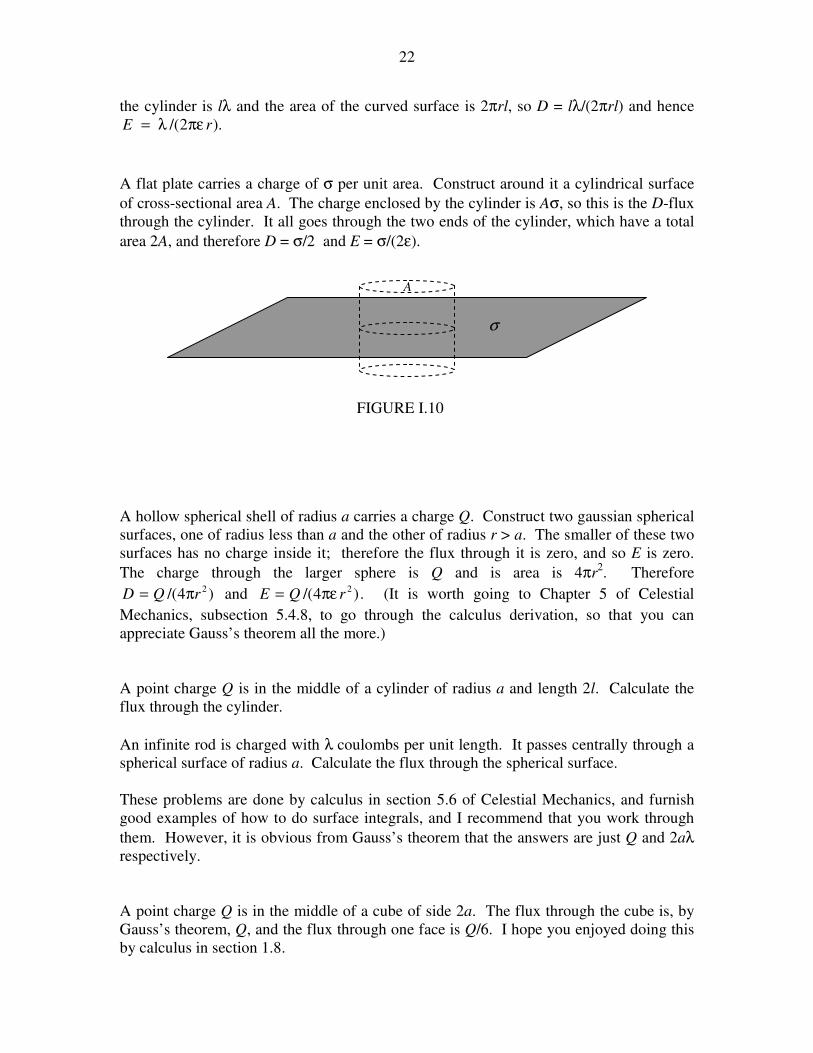
A flat plate carries a charge of σ per unit area. Construct around it a cylindrical surface

of cross-sectional area A. The charge enclosed by the cylinder is Aσ, so this is the D-flux

through the cylinder. It all goes through the two ends of the cylinder, which have a total

area 2A, and therefore D = σ/2 and E = σ/(2ε).

A hollow spherical shell of radius a carries a charge Q. Construct two gaussian spherical

surfaces, one of radius less than a and the other of radius r > a. The smaller of these two

surfaces has no charge inside it; therefore the flux through it is zero, and so E is zero.

The charge through the larger sphere is Q and is area is 4πr2. Therefore

.)4/(and)4/( 22rQErQD πε=π= (It is worth going to Chapter 5 of Celestial

Mechanics, subsection 5.4.8, to go through the calculus derivation, so that you can

appreciate Gauss’s theorem all the more.)

A point charge Q is in the middle of a cylinder of radius a and length 2l. Calculate the

flux through the cylinder.

An infinite rod is charged with λ coulombs per unit length. It passes centrally through a

spherical surface of radius a. Calculate the flux through the spherical surface.

These problems are done by calculus in section 5.6 of Celestial Mechanics, and furnish

good examples of how to do surface integrals, and I recommend that you work through

them. However, it is obvious from Gauss’s theorem that the answers are just Q and 2aλ

respectively.

A point charge Q is in the middle of a cube of side 2a. The flux through the cube is, by

Gauss’s theorem, Q, and the flux through one face is Q/6. I hope you enjoyed doing this

by calculus in section 1.8.

A

σ

FIGURE I.10

1

CHAPTER 2

ELECTROSTATIC POTENTIAL

2.1 Introduction

Imagine that some region of space, such as the room you are sitting in, is permeated by

an electric field. (Perhaps there are all sorts of electrically charged bodies outside the

room.) If you place a small positive test charge somewhere in the room, it will

experience a force F = QE. If you try to move the charge from point A to point B

against the direction of the electric field, you will have to do work. If work is required to

move a positive charge from point A to point B, there is said to be an electrical potential

difference between A and B, with point A being at the lower potential. If one joule of

work is required to move one coulomb of charge from A to B, the potential difference

between A and B is one volt (V).

The dimensions of potential difference are ML2T

−2Q

−1.

All we have done so far is to define the potential difference between two points. We

cannot define “the” potential at a point unless we arbitrarily assign some reference point

as having a defined potential. It is not always necessary to do this, since we are often

interested only in the potential differences between point, but in many circumstances it is

customary to define the potential to be zero at an infinite distance from any charges of

interest. We can then say what “the” potential is at some nearby point. Potential and

potential difference are scalar quantities.

Suppose we have an electric field E in the positive x-direction (towards the right). This

means that potential is decreasing to the right. You would have to do work to move a

positive test charge Q to the left, so that potential is increasing towards the left. The

force on Q is QE, so the work you would have to do to move it a distance dx to the right

is −QE dx, but by definition this is also equal to Q dV, where dV is the potential

difference between x and x + dx.

Therefore .dx

dVE −= 2.1.1

In a more general three-dimensional situation, this is written

.

∂

∂+

∂

∂+

∂

∂−=−=−=

x

V

x

V

x

VVV kjigradE ∇∇∇∇ 2.1.2

We see that, as an alternative to expressing electric field strength in newtons per

coulomb, we can equally well express it in volts per metre (V m−1

).

The inverse of equation 2.1.1 is, of course,

2

.constant+−= ∫ dxEV 2.1.3

2.2 Potential Near Various Charged Bodies

2.2.1 Point Charge

Let us arbitrarily assign the value zero to the potential at an infinite distance from a point

charge Q. “The” potential at a distance r from this charge is then the work required to

move a unit positive charge from infinity to a distance r.

At a distance x from the charge, the field strength is .4 2

0 x

Q

πε The work required to

move a unit charge from x to x + δx is 2

04 x

xQ

πε

δ− . The work required to move unit

charge from r to infinity is .44 0

2

0 r

Q

x

dxQ

r πε−=

πε− ∫

∞

The work required to move unit

charge from infinity to r is minus this.

Therefore .4 0 r

QV

πε+= 2.2.1

The mutual potential energy of two charges Q1 and Q2 separated by a distance r is the

work required to bring them to this distance apart from an original infinite separation.

This is

.4

P.E.0

21

r

QQ

πε+= 2.2.2

Before proceeding, a little review is in order.

Field at a distance r from a charge Q:

,4 2

0 r

QE

πε= N C

−1 or V m

−1

or, in vector form, .4

ˆ4 3

0

2

0

rrEr

Q

r

Q

πε=

πε= N C

−1 or V m

−1

3

Force between two charges, Q1 and Q2:

.4 2

21

r

QQF

πε= N

Potential at a distance r from a charge Q:

.4 0 r

QV

πε= V

Mutual potential energy between two charges:

.4

P.E.0

21

r

QQ

πε= J

We couldn’t possibly go wrong with any of these, could we?


Outside any spherically-symmetric charge distribution, the field is the same as if all the

charge were concentrated at a point in the centre, and so, then, is the potential. Thus

.4 0 r

QV

πε= 2.2.3

Inside a hollow spherical shell of radius a and carrying a charge Q the field is zero, and

therefore the potential is uniform throughout the interior, and equal to the potential on the

surface, which is

.4 0 a

QV

πε= 2.2.4

A solid sphere of radius a bearing a charge Q that is uniformly distributed throughout the

sphere is easier to imagine than to achieve in practice, but, for all we know, a proton

might be like this (it might be – but it isn’t!), so let’s calculate the field at a point P inside

the sphere at a distance r (< a) from the centre. See figure II.1

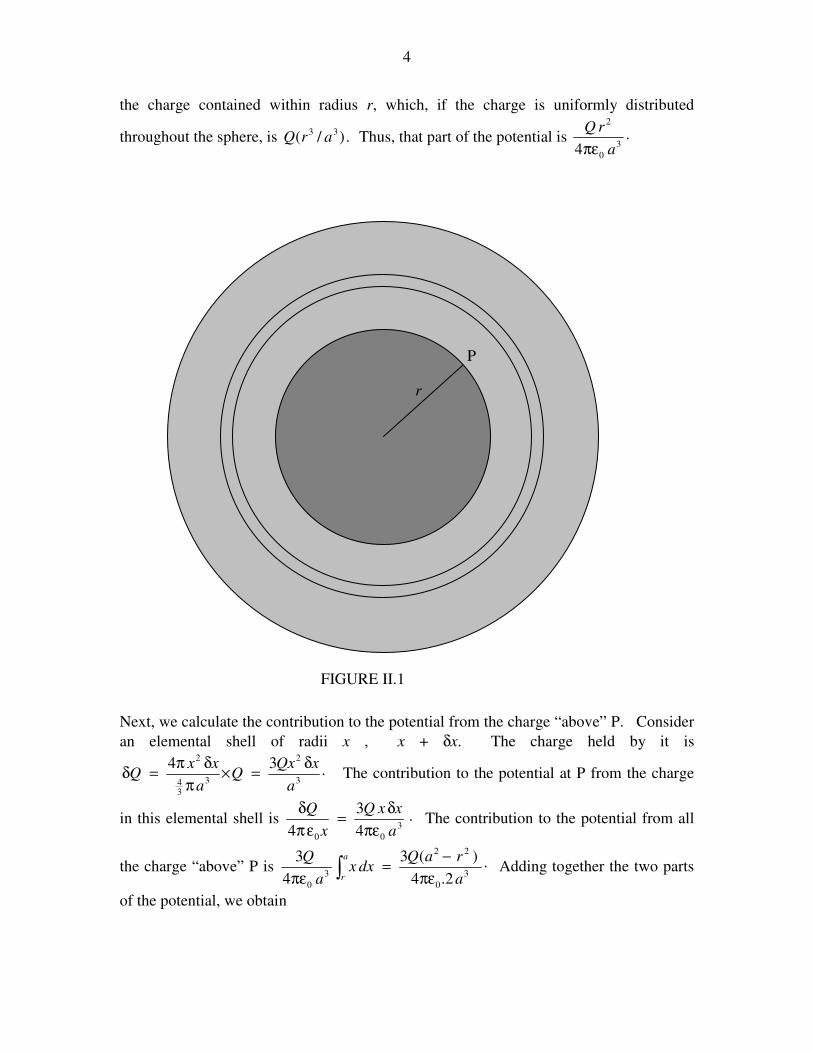
We can do this in two parts. First the potential from the part of the sphere “below” P. If

the charge is uniformly distributed throughout the sphere, this is just .4 0 r

Qr

πε Here Qr is

4

the charge contained within radius r, which, if the charge is uniformly distributed

throughout the sphere, is .)/( 33arQ Thus, that part of the potential is .

4 3

0

2

a

rQ

πε

Next, we calculate the contribution to the potential from the charge “above” P. Consider

an elemental shell of radii x , x + δx. The charge held by it is

.343

2

3

34

2

a

xQxQ

a

xxQ

δ=×

π

δπ=δ The contribution to the potential at P from the charge

in this elemental shell is .4

3

4 3

00 a

xxQ

x

Q

πε

δ=

επ

δ The contribution to the potential from all

the charge “above” P is .2.4

)(3

4

33

0

22

3

0 a

raQdxx

a

Q a

r πε

−=

πε ∫ Adding together the two parts

of the potential, we obtain

r

P

FIGURE II.1

5

.)3(8

22

3

0

raa

QV −

πε= 2.2.5

2.2.3 Long Charged Rod

The field at a distance r from a long charged rod carrying a charge λ coulombs per metre

is .2 0 rπε

λ Therefore the potential difference between two points at distances a and b

from the rod (a < b) is

.2 0

∫πε

λ−=−

b

aab

r

drVV

â .)/ln(2 0

abVVba

πε

λ=− 2.2.6

2.2.4 Large Plane Charged Sheet

The field at a distance r from a large charged sheet carrying a charge σ coulombs per

square metre is .2 0ε

σ Therefore the potential difference between two points at distances

a and b from the sheet (a < b) is

.)(2 0

abVVba

−ε

σ=− 2.2.7

2.2.5 Potential on the Axis of a Charged Ring

The field on the axis of a charged ring is given in section 1.6.4. The reader is invited to

show that the potential on the axis of the ring is

.)(4 2/122

0 xa

QV

+πε= 2.2.8

You can do this either by integrating the expression for the field or just by thinking about

it for a few seconds and realizing that potential is a scalar quantity.

6

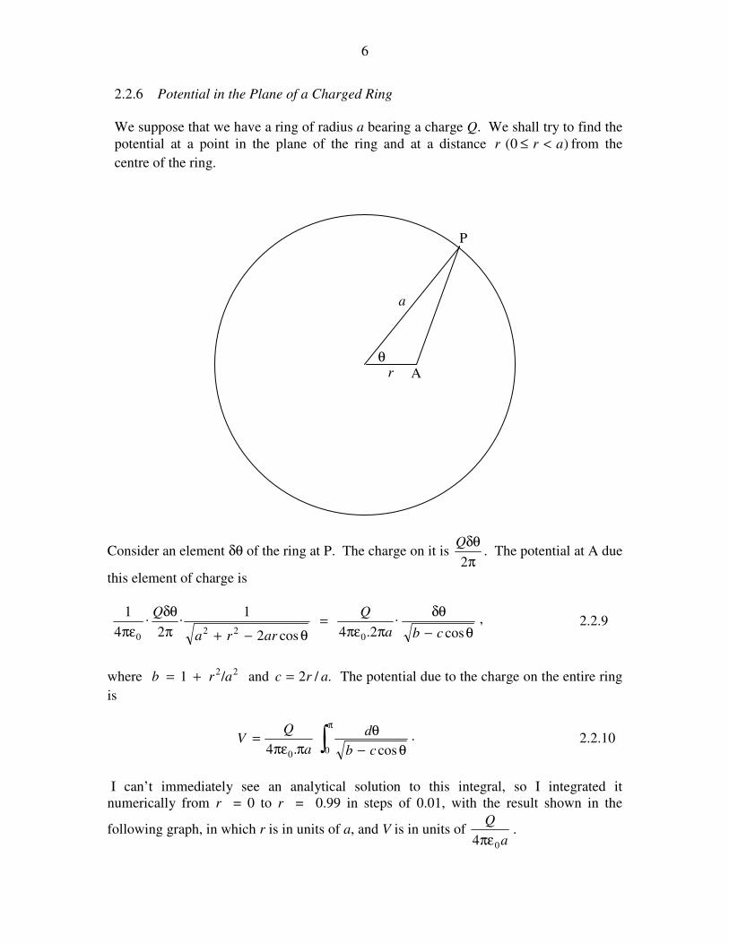
2.2.6 Potential in the Plane of a Charged Ring

We suppose that we have a ring of radius a bearing a charge Q. We shall try to find the

potential at a point in the plane of the ring and at a distance )0( arr <≤ from the

centre of the ring.

Consider an element δθ of the ring at P. The charge on it is π

δθ

2

Q. The potential at A due

this element of charge is

,cos

.2.4cos2

1.2

.4

1

022

0 θ−

δθ

ππε=

θ−+π

δθ

πε cba

Q

arra

Q 2.2.9

where 22/1 arb += and ./2 arc = The potential due to the charge on the entire ring

is

.cos.4 00 θ−

θ

ππε=

π

∫ cb

d

a

QV 2.2.10

I can’t immediately see an analytical solution to this integral, so I integrated it

numerically from r = 0 to r = 0.99 in steps of 0.01, with the result shown in the

following graph, in which r is in units of a, and V is in units of .4 0a

Q

πε

θ A

P

a

r

7

0 0.1 0.2 0.3 0.4 0.5 0.6 0.7 0.8 0.9 10

0.5

1

1.5

2

r

V

The field is equal to the gradient of this and is directed towards the centre of the ring. It

looks as though a small positive charge would be in stable equilibrium at the centre of the

ring, and this would be so if the charge were constrained to remain in the plane of the

ring. But, without such a constraint, the charge would be pushed away from the ring if it

strayed at all above or below the plane of the ring.

Some computational notes.

Any reader who has tried to reproduce these results will have discovered that rather a

lot of heavy computation is required. Since there is no simple analytical expression for

the integration, each of the 100 points from which the graph was computed entailed a

numerical integration of the expression for the potential. I found that Simpson’s Rule did

not give very satisfactory results, mainly because of the steep rise in the function at large

r, so I used Gaussian quadrature, which proved much more satisfactory.

Can we avoid the numerical integration? One possibility is to express the integrand in

equation 2.2.10 as a power series in cos θ, and then integrate term by term.

Thus θ−=θ− cos1.cos ebcb , where .1)/(

)/(22 +

==ar

ar

b

ce And then

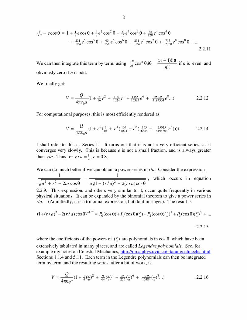
8

...coscoscoscos

coscoscoscos1cos1

88

3276871577

102423166

2566355

1024231

44

1283533

16522

83

21

+θ+θ+θ+θ+

θ+θ+θ+θ+=θ−

eeee

eeeee

2.2.11

We can then integrate this term by term, using !!

!)!1(cos

0n

nd

n π−=θθ∫

π if n is even, and

obviously zero if n is odd.

We finally get:

...).1(4

8

4194304250256

1638411554

10241052

163

0

eeeea

QV ++++

πε= 2.2.12

For computational purposes, this is most efficiently rendered as

)))).(((1(4

8

419430425025

1638411556

10241054

1632

0

eeeea

QV ++++

πε= 2.2.14

I shall refer to this as Series I. It turns out that it is not a very efficient series, as it

converges very slowly. This is because e is not a small fraction, and is always greater

than r/a. Thus for .8.0,/21 == ear

We can do much better if we can obtain a power series in r/a. Consider the expression

θ−+=

θ−+ cos)/(2)/(1

1

cos2

1

222araraarra

, which occurs in equation

2.2.9. This expression, and others very similar to it, occur quite frequently in various

physical situations. It can be expanded by the binomial theorem to give a power series in

r/a. (Admittedly, it is a trinomial expression, but do it in stages). The result is

...))((cos))((cos))((cos)(cos)cos)/(2)/(1( 33

2210

2/12 +θ+θ+θ+θ=θ−+ −a

r

a

r

a

rPPPParar

2.2.15

where the coefficients of the powers of )(a

r are polynomials in cos θ, which have been

extensively tabulated in many places, and are called Legendre polynomials. See, for

example my notes on Celestial Mechanics, http://orca.phys.uvic.ca/~tatum/celmechs.html

Sections 1.1.4 and 5.11. Each term in the Legendre polynomials can then be integrated

term by term, and the resulting series, after a bit of work, is

...).)()()()(1(4

8

1638412256

256254

6492

41

0a

r

a

r

a

r

a

r

a

QV ++++

πε= 2.2.16

9

Since this is a series in )(a

r rather than is e, it converges much faster than equation 2.2.13.

I shall refer to it as series II. Of course, for computational purposes it should be written

with nested parentheses, as we did for series I in equation 2.2.14.

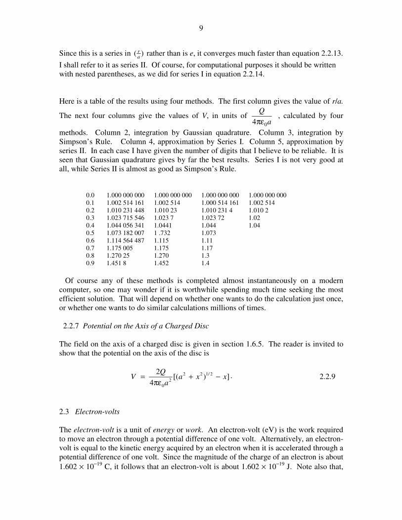
Here is a table of the results using four methods. The first column gives the value of r/a.

The next four columns give the values of V, in units of a

Q

04πε, calculated by four

methods. Column 2, integration by Gaussian quadrature. Column 3, integration by

Simpson’s Rule. Column 4, approximation by Series I. Column 5, approximation by

series II. In each case I have given the number of digits that I believe to be reliable. It is

seen that Gaussian quadrature gives by far the best results. Series I is not very good at

all, while Series II is almost as good as Simpson’s Rule.

0.0 1.000 000 000 1.000 000 000 1.000 000 000 1.000 000 000

0.1 1.002 514 161 1.002 514 1.000 514 161 1.002 514

0.2 1.010 231 448 1.010 23 1.010 231 4 1.010 2

0.3 1.023 715 546 1.023 7 1.023 72 1.02

0.4 1.044 056 341 1.0441 1.044 1.04

0.5 1.073 182 007 1 .732 1.073

0.6 1.114 564 487 1.115 1.11

0.7 1.175 005 1.175 1.17

0.8 1.270 25 1.270 1.3

0.9 1.451 8 1.452 1.4

Of course any of these methods is completed almost instantaneously on a modern

computer, so one may wonder if it is worthwhile spending much time seeking the most

efficient solution. That will depend on whether one wants to do the calculation just once,

or whether one wants to do similar calculations millions of times.

2.2.7 Potential on the Axis of a Charged Disc

The field on the axis of a charged disc is given in section 1.6.5. The reader is invited to

show that the potential on the axis of the disc is

.])[(4

2 2/122

2

0

xxaa

QV −+

πε= 2.2.9

2.3 Electron-volts

The electron-volt is a unit of energy or work. An electron-volt (eV) is the work required

to move an electron through a potential difference of one volt. Alternatively, an electron-

volt is equal to the kinetic energy acquired by an electron when it is accelerated through a

potential difference of one volt. Since the magnitude of the charge of an electron is about

1.602 × 10−19

C, it follows that an electron-volt is about 1.602 × 10−19

J. Note also that,

10

because the charge on an electron is negative, it requires work to move an electron from a

point of high potential to a point of low potential.

Exercise. If an electron is accelerated through a potential difference of a million volts,

its kinetic energy is, of course, 1 MeV. At what speed is it then moving?

First attempt. .2

21

eVm =v

(Here eV, written in italics, is not intended to mean the unit electron-volt, but e is the

magnitude of the electron charge, and V is the potential difference (106 volts) through

which it is accelerated.) Thus ./2 meV=v With m = 9.109 × 10−31

kg, this comes

to v = 5.9 × 108 m s

−1. Oops! That looks awfully fast! We’d better do it properly this

time.

Second attempt. .)1( 2eVmc =−γ

Some readers will know exactly what we are doing here, without explanation. Others

may be completely mystified. For the latter, the difficulty is that the speed that we had

calculated was even greater than the speed of light. To do this properly we have to use

the formulas of special relativity. See, for example, Chapter 15 of the Classical

Mechanics section of these notes.

At any rate, this results in γ = 2.958, whence β = 0.9411 and v = 2.82 × 108 m s

−1.

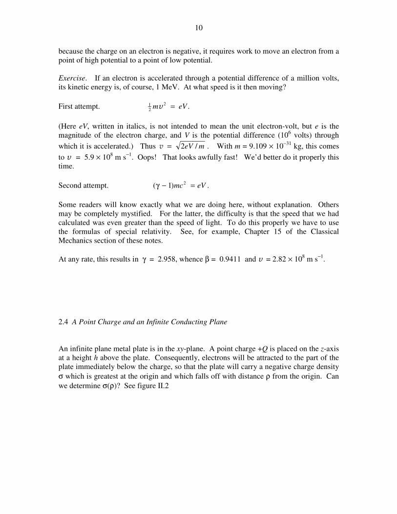
2.4 A Point Charge and an Infinite Conducting Plane

An infinite plane metal plate is in the xy-plane. A point charge +Q is placed on the z-axis

at a height h above the plate. Consequently, electrons will be attracted to the part of the

plate immediately below the charge, so that the plate will carry a negative charge density

σ which is greatest at the origin and which falls off with distance ρ from the origin. Can

we determine σ(ρ)? See figure II.2

11

First, note that the metal surface, being a conductor, is an equipotential surface, as is any

metal surface. The potential is uniform anywhere on the surface. Now suppose that,

instead of the metal surface, we had (in addition to the charge +Q at a height h above the

xy-plane), a second point charge, −Q, at a distance h below the xy-plane. The potential in

the xy-plane would, by symmetry, be uniform everywhere. That is to say that the

potential in the xy-plane is the same as it was in the case of the single point charge and

the metal plate, and indeed the potential at any point above the plane is the same in both

cases. For the purpose of calculating the potential, we can replace the metal plate by an

image of the point charge. It is easy to calculate the potential at a point (z , ρ). If we

suppose that the permittivity above the plate is ε0, the potential at (z , ρ) is

.])([

1

])([

1

4 2/1222/122

0

++ρ−

−+ρπε=

zhzh

QV 2.4.1

The field strength E in the xy-plane is −∂ ∂V z/ evaluated at z = 0, and this is

EQ h

h= −

+

2

4 0

2 2 3 2πε ρ.( )

./

2.4.2

The D-field is ε0 times this, and since all the lines of force are above the metal plate,

Gauss's theorem provides that the charge density is σ = D, and hence the charge density

is

σπ ρ

= −+

Q h

h2 2 2 3 2.( )

./

2.4.3

− − − − − − − − − −−− − − − − − − − − −

+Q

h

ρ

σ

FIGURE II.2

12

This can also be written σπ ξ

= −Q h

2 3. , 2.4.4

where ξ ρ2 2 2= + h , with obvious geometric interpretation.

Exercise: How much charge is there on the surface of the plate within an annulus

bounded by radii ρ and ρ + dρ? Integrate this from zero to infinity to show that the

total charge induced on the plate is −Q.

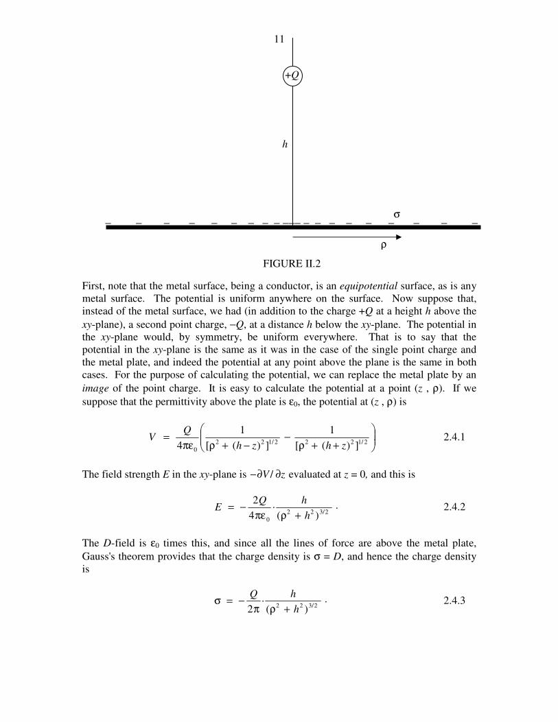
2.5 A Point Charge and a Conducting Sphere

A point charge +Q is at a distance R from a metal sphere of radius a. We are going to try

to calculate the surface charge density induced on the surface of the sphere, as a function

of position on the surface. We shall bear in mind that the surface of the sphere is an

equipotential surface, and we shall take the potential on the surface to be zero.

Let us first construct a point I such that the triangles OPI and PQO are similar, with the

lengths shown in figure II.3. The length OI is a2/R. Then R a/ / ,ξ ζ= or

1

0ξ ζ

− =a R/

. 2.5.1

This relation between the variables ξ and ζ is in effect the equation to the sphere

expressed in these variables.

Now suppose that, instead of the metal sphere, we had (in addition to the charge +Q at a

distance R from O), a second point charge −(a/R)Q at I. The locus of points where the

potential is zero is where

+Q O

P

a

R

ξ

I

ζ

FIGURE II.3

13

.0/1

4 0

=

ζ−

ξπε

RaQ 2.5.2

That is, the surface of our sphere. Thus, for purposes of calculating the potential, we can

replace the metal sphere by an image of Q at I, this image carrying a charge of −(a/R)Q.

Let us take the line OQ as the z-axis of a coordinate system. Let X be some point such

that OX = r and the angle XOQ = θ. The potential at P from a charge +Q at Q and a

charge −(a/R)Q at I is (see figure II.4)

.)/cos2/(

/

)cos2(

1

4 2/122422/122

0

θ−+−

θ−+πε=

RraRar

Ra

rRRr

QV 2.5.2

The E field on the surface of the sphere is −∂ ∂V r/ evaluated at r = a. The D field is ε0

times this, and the surface charge density is equal to D. After some patience and algebra,

we obtain, for a point X on the surface of the sphere

.)XQ(

1..4 3

22

a

aRQ −

π−=σ 2.5.3

+Q O

X

I

FIGURE II.4

r

OI = a2/R

14

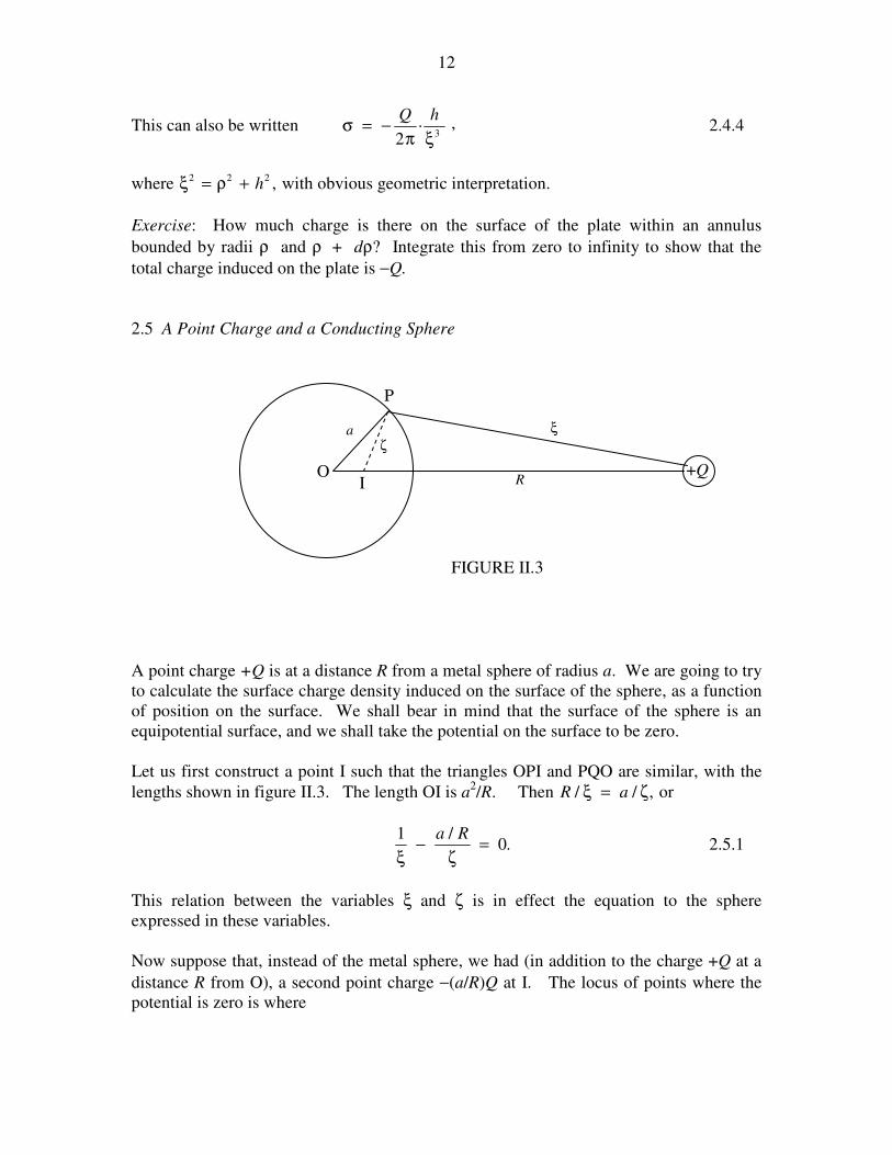
2.6 Two Semicylindrical Electrodes

This section requires that the reader should be familiar with functions of a complex

variable and conformal transformations. For readers not familiar with these, this section

can be skipped without prejudice to understanding following chapters. For readers who

are familiar, this is a nice example of conformal transformations to solve a physical

problem.

We have two semicylindrical electrodes as shown in figure II.5. The potential of the

upper one is 0 and the potential of the lower one is V0. We'll suppose the radius of the

curcle is 1; or, what amounts to the same thing, we'll express coordinates x and y in units

of the radius. Let us represent the position of any point whose coordinates are (x , y) by a

complex number z = x + iy.

Now let w = u + iv be a complex number related to z by ;1

1

+

−=

z

ziw that is,

ziw

iw=

+

−

1

1. Substitute w = u + iv and z = x + iy in each of these equations, and equate

real and imaginary parts, to obtain

V = 0

V = V0

x

y

FIGURE II.5

O B

A

15

uy

x y

x y

x y=

+ +=

− −

+ +

2

1

1

12 2

2 2

2 2( );

( );v 2.6.1

xu

uy

u

u=

− −

+ +=

+ +

1

1

2

1

2 2

2 2 2 2

v

v v( );

( ). 2.6.2

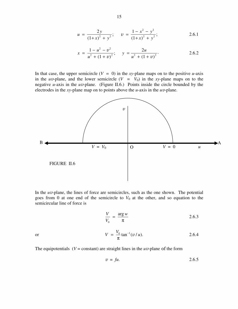
In that case, the upper semicircle (V = 0) in the xy-plane maps on to the positive u-axis

in the uv-plane, and the lower semicircle (V = V0) in the xy-plane maps on to the

negative u-axis in the uv-plane. (Figure II.6.) Points inside the circle bounded by the

electrodes in the xy-plane map on to points above the u-axis in the uv-plane.

In the uv-plane, the lines of force are semicircles, such as the one shown. The potential

goes from 0 at one end of the semicircle to V0 at the other, and so equation to the

semicircular line of force is

V

V

w

0

=arg

π 2.6.3

or VV

u= −0 1

πtan ( / ).v 2.6.4

The equipotentials (V = constant) are straight lines in the uv-plane of the form

v = fu. 2.6.5

B

v

u O A

FIGURE II.6

V = V0 V = 0

16

(You would prefer me to use the symbol m for the slope of the equipotentials, but in a

moment you will be glad that I chose the symbol f.)

If we now transform back to the xy-plane, we see that the equation to the lines of force is

,2

1tan

2210

−−

π= −

y

yxVV 2.6.6

and the equation to the equipotentials is

1 22 2− − =x y fy , 2.6.7

or x y fy2 2 2 1 0+ + − = . 2.6.8

Now aren't you glad that I chose f ? Those who are handy with conic sections (see

Chapter 2 of Celestial Mechanics) will understand that the equipotentials in the xy-plane

are circles of radii f2 1+ , whose centres are at (0 , ! f ), and which all pass through the

points (!1 , 0). They are drawn as blue lines in figure II.7. The lines of force are the

orthogonal trajectories to these, and are of the form

x y gy2 2 2 1 0+ + + = . 2.6.9

These are circles of radii g2 1− and have their centres at (0 , ! g). They are shown as

dashed red lines in figure II.7.

FIGURE II.7

1

CHAPTER 3

DIPOLE AND QUADRUPOLE MOMENTS

3.1 Introduction

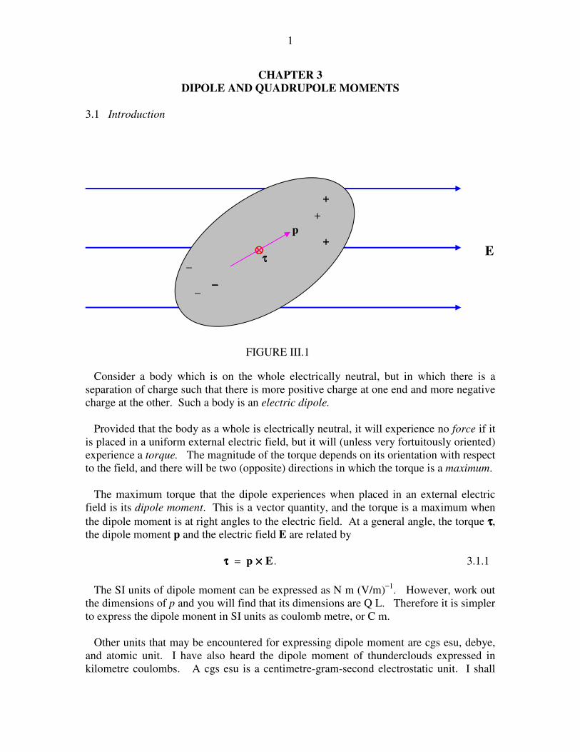
Consider a body which is on the whole electrically neutral, but in which there is a

separation of charge such that there is more positive charge at one end and more negative

charge at the other. Such a body is an electric dipole.

Provided that the body as a whole is electrically neutral, it will experience no force if it

is placed in a uniform external electric field, but it will (unless very fortuitously oriented)

experience a torque. The magnitude of the torque depends on its orientation with respect

to the field, and there will be two (opposite) directions in which the torque is a maximum.

The maximum torque that the dipole experiences when placed in an external electric

field is its dipole moment. This is a vector quantity, and the torque is a maximum when

the dipole moment is at right angles to the electric field. At a general angle, the torque ττττ,

the dipole moment p and the electric field E are related by

.Ep ××××ττττ = 3.1.1

The SI units of dipole moment can be expressed as N m (V/m)−1

. However, work out

the dimensions of p and you will find that its dimensions are Q L. Therefore it is simpler

to express the dipole monent in SI units as coulomb metre, or C m.

Other units that may be encountered for expressing dipole moment are cgs esu, debye,

and atomic unit. I have also heard the dipole moment of thunderclouds expressed in

kilometre coulombs. A cgs esu is a centimetre-gram-second electrostatic unit. I shall

1111

+

+

−

− −−−−

+

ττττ

p

E

FIGURE III.1

2

describe the cgs esu system in a later chapter; suffice it here to say that a cgs esu of

dipole moment is about 3.336 × 10−12

C m, and a debye (D) is 10−18

cgs esu. An atomic

unit of electric dipole moment is a0e, where a0 is the radius of the first Bohr orbit for

hydrogen and e is the magnitude of the electronic charge. An atomic unit of dipole

moment is about 8.478 × 10−29

C m.

I remark in passing that I have heard, distressingly often, some such remark as “The molecule has a

dipole”. Since this sentence is not English, I do not know what it is intended to mean. It would be English

to say that a molecule is a dipole or that it has a dipole moment.

3.2 Mathematical Definition of Dipole Moment

In the introductory section 3.1 we gave a physical definition of dipole moment. I am

now about to give a mathematical definition.

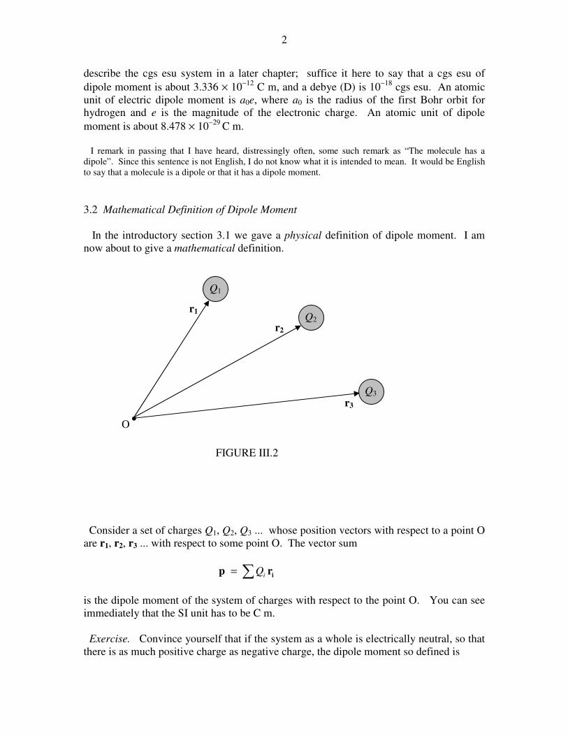
Consider a set of charges Q1, Q2, Q3 ... whose position vectors with respect to a point O

are r1, r2, r3 ... with respect to some point O. The vector sum

∑=i

rpi

Q

is the dipole moment of the system of charges with respect to the point O. You can see

immediately that the SI unit has to be C m.

Exercise. Convince yourself that if the system as a whole is electrically neutral, so that

there is as much positive charge as negative charge, the dipole moment so defined is

Q1

Q2

Q3

•O

r1

r2

r3

FIGURE III.2

3

independent of the position of the point O. One can then talk of “the dipole moment of

the system” without adding the rider “with respect to the point O”.

Exercise. Convince yourself that if any electrically neutral system is placed in an

external electric field E, it will experience a torque given by Epτ ××××= , and so the two

definitions of dipole moment − the physical and the mathematical – are equivalent.

Exercise. While thinking about these two, also convince yourself (from mathematics

or from physics) that the moment of a simple dipole consisting of two charges, +Q and

−Q separated by a distance l is Ql. We have already noted that C m is an acceptable SI

unit for dipole moment.

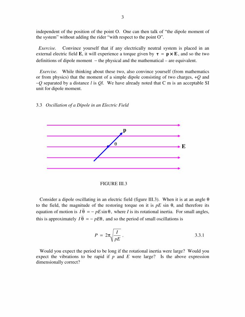
3.3 Oscillation of a Dipole in an Electric Field

Consider a dipole oscillating in an electric field (figure III.3). When it is at an angle θ

to the field, the magnitude of the restoring torque on it is pE sin θ, and therefore its

equation of motion is ,sin θ−=θ pEI && where I is its rotational inertia. For small angles,

this is approximately ,θ−=θ pEI && and so the period of small oscillations is

.2pE

IP π= 3.3.1

Would you expect the period to be long if the rotational inertia were large? Would you

expect the vibrations to be rapid if p and E were large? Is the above expression

dimensionally correct?

•

p

E θ

FIGURE III.3

4

3.4 Potential Energy of a Dipole in an Electric Field

Refer again to figure III.3. There is a torque on the dipole of magnitude pE sin θ. In

order to increase θ by δθ you would have to do an amount of work pE sin θ δθ . The

amount of work you would have to do to increase the angle between p and E from 0 to θ

would be the integral of this from 0 to θ, which is pE(1 − cos θ), and this is the potential

energy of the dipole, provided one takes the potential energy to be zero when p and E are

parallel. In many applications, writers find it convenient to take the potential energy

(P.E.) to be zero when p and E perpendicular. In that case, the potential energy is

.cosP.E. Ep •−=θ−= pE 3.4.1

This is negative when θ is acute and positive when θ is obtuse. You should verify that

the product of p and E does have the dimensions of energy.

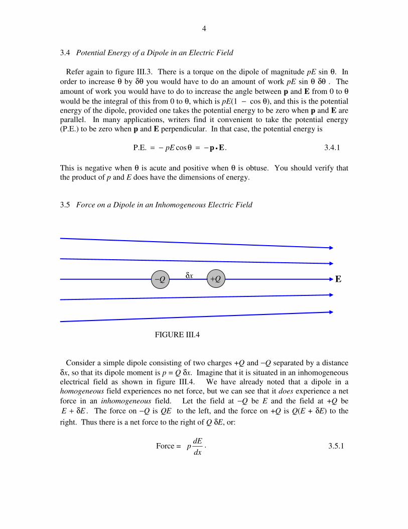
3.5 Force on a Dipole in an Inhomogeneous Electric Field

Consider a simple dipole consisting of two charges +Q and −Q separated by a distance

δx, so that its dipole moment is p = Q δx. Imagine that it is situated in an inhomogeneous

electrical field as shown in figure III.4. We have already noted that a dipole in a

homogeneous field experiences no net force, but we can see that it does experience a net

force in an inhomogeneous field. Let the field at −Q be E and the field at +Q be

.EE δ+ The force on −Q is QE to the left, and the force on +Q is Q(E + δE) to the

right. Thus there is a net force to the right of Q δE, or:

Force = .dx

dEp 3.5.1

−Q +Q δx

E

FIGURE III.4

5

Equation 3.5.1 describes the situation where the dipole, the electric field and the

gradient are all parallel to the x-axis. In a more general situation, all three of these are in

different directions. Recall that electric field is minus potential gradient. Potential is a

scalar function, whereas electric field is a vector function with three component, of which

the x-component, for example is .x

VE

x

∂

∂−= Field gradient is a symmetric tensor

having nine components (of which, however, only six are distinct), such as ,,2

2

2

zy

V

x

V

∂∂

∂

∂

∂

etc. Thus in general equation 3.5.1 would have to be written as

,

−=

z

y

x

zzyzxz

yzyyxy

xzxyxx

z

y

x

p

p

p

VVV

VVV

VVV

E

E

E

3.5.2

in which the double subscripts in the potential gradient tensor denote the second partial

derivatives.

3.6 Induced Dipoles and Polarizability

We noted in section 1.3 that a charged rod will attract an uncharged pith ball, and at that

time we left this as a little unsolved mystery. What happens is that the rod induces a

dipole moment in the uncharged pith ball, and the pith ball, which now has a dipole

moment, is attracted in the inhomogeneous field surrounding the charged rod.

How may a dipole moment be induced in an uncharged body? Well, if the uncharged

body is metallic (as in the gold leaf electroscope), it is quite easy. In a metal, there are

numerous free electrons, not attached to any particular atoms, and they are free to wander

about inside the metal. If a metal is placed in an electric field, the free electrons are

attracted to one end of the metal, leaving an excess of positive charge at the other end.

Thus a dipole moment is induced.

What about a nonmetal, which doesn’t have free electrons unattached to atoms? It may

be that the individual molecules in the material have permanent dipole moments. In that

case, the imposition of an external electric field will exert a torque on the molecules, and

will cause all their dipole moments to line up in the same direction, and thus the bulk

material will acquire a dipole moment. The water molecule, for example, has a

permanent dipole moment, and these dipoles will align in an external field. This is why

pure water has such a large dielectric constant.

But what if the molecules do not have a permanent dipole moment, or what if they do,

but they cannot easily rotate (as may well be the case in a solid material)? The bulk

material can still become polarized, because a dipole moment is induced in the individual

molecules, the electrons inside the molecule tending to be pushed towards one end of the

molecule. Or a molecule such as CH4, which is symmetrical in the absence of an external

6

electric field, may become distorted from its symmetrical shape when placed in an

electric field, and thereby acquire a dipole moment.

Thus, one way or another, the imposition of an electric field may induce a dipole

moment in most materials, whether they are conductors of electricity or not, or whether

or not their molecules have permanent dipole moments.

If two molecules approach each other in a gas, the electrons in one molecule repel the

electrons in the other, so that each molecule induces a dipole moment in the other. The

two molecules then attract each other, because each dipolar molecule finds itself in the

inhomogeneous electric field of the other. This is the origin of the van der Waals forces.

Some bodies (I am thinking about individual molecules in particular, but this is not

necessary) are more easily polarized that others by the imposition of an external field.

The ratio of the induced dipole moment to the applied field is called the polarizability

α of the molecule (or whatever body we have in mind). Thus

.Eα=p 3.6.1

The SI unit for α is C m (V m−1

) −1

and the dimensions are M−1

T2Q

2.

This brief account, and the general appearance of equation 3.6.1, suggests that p and E

are in the same direction – but this is so only if the electrical properties of the molecule

are isotropic. Perhaps most molecules – and, especially, long organic molecules − have

anisotropic polarizability. Thus a molecule may be easy to polarize with a field in the x-

direction, and much less easy in the y- or z-directions. Thus, in equation 3.6.1, the

polarizability is really a symmetric tensor, p and E are not in general parallel, and the

equation, written out in full, is

.

ααα

ααα

ααα

=

z

y

x

zzyzxz

yzyyxy

xzxyxx

z

y

x

E

E

E

p

p

p

3.6.2

(Unlike in equation 3.5.2, the double subscripts are not intended to indicate second partial

derivatives; rather they are just the components of the polarizability tensor.) As in

several analogous situations in various branches of physics (see, for example, section

2.17 of Classical Mechanics and the inertia tensor) there are three mutually orthogonal

directions (the eigenvectors of the polarizability tensor) for which p and E will be

parallel.

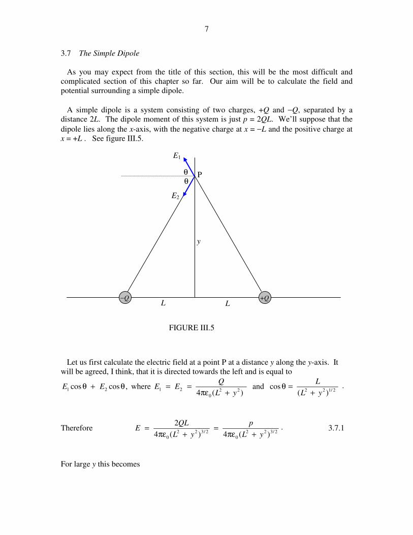
7

3.7 The Simple Dipole

As you may expect from the title of this section, this will be the most difficult and

complicated section of this chapter so far. Our aim will be to calculate the field and

potential surrounding a simple dipole.

A simple dipole is a system consisting of two charges, +Q and −Q, separated by a

distance 2L. The dipole moment of this system is just p = 2QL. We’ll suppose that the

dipole lies along the x-axis, with the negative charge at x = −L and the positive charge at

x = +L . See figure III.5.

Let us first calculate the electric field at a point P at a distance y along the y-axis. It

will be agreed, I think, that it is directed towards the left and is equal to

,coscos 21 θ+θ EE where .)(

cosand)(4 2/12222

0

21yL

L

yL

QEE

+=θ

+πε==

Therefore .)(4)(4

22/322

0

2/322

0 yL

p

yL

QLE

+πε=

+πε= 3.7.1

For large y this becomes

−Q +Q L L

E1

y

E2

P

FIGURE III.5

θ

θ

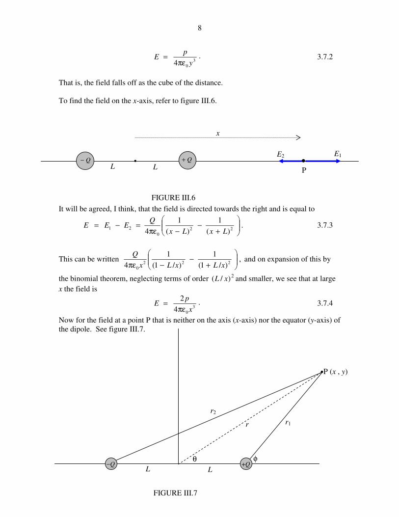
8

.4 3

0 y

pE

πε= 3.7.2

That is, the field falls off as the cube of the distance.

To find the field on the x-axis, refer to figure III.6.

It will be agreed, I think, that the field is directed towards the right and is equal to

.)(

1

)(

1

4 22

0

21

+−

−πε=−=

LxLx

QEEE 3.7.3

This can be written ,)/1(

1

)/1(

1

4 222

0

+−

−πε xLxLx

Q and on expansion of this by

the binomial theorem, neglecting terms of order 2)/( xL and smaller, we see that at large

x the field is

.4

23

0x

pE

πε= 3.7.4

Now for the field at a point P that is neither on the axis (x-axis) nor the equator (y-axis) of

the dipole. See figure III.7.

− Q + Q

L •

L P

x

FIGURE III.6

• E1 E2

•P (x , y)

−Q +Q L L

FIGURE III.7

r1

r2

r

θ φ

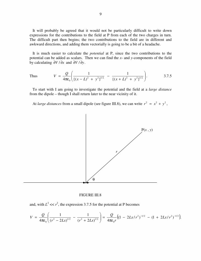
9

It will probably be agreed that it would not be particularly difficult to write down

expressions for the contributions to the field at P from each of the two charges in turn.

The difficult part then begins; the two contributions to the field are in different and

awkward directions, and adding them vectorially is going to be a bit of a headache.

It is much easier to calculate the potential at P, since the two contributions to the

potential can be added as scalars. Then we can find the x- and y-components of the field

by calculating xV ∂∂ / and ./ yV ∂∂

Thus .)(

1

)(

1

4 2/1222/122

0

++−

+−πε=

yLxyLx

QV 3.7.5

To start with I am going to investigate the potential and the field at a large distance

from the dipole – though I shall return later to the near vicinity of it.

At large distances from a small dipole (see figure III.8), we can write ,222yxr +=

and, with L2 << r

2, the expression 3.7.5 for the potential at P becomes

( ).)/21()/21(4)2(

1

)2(

1

4

2/122/12

0

2/122/12

0

−− +−−πε

=

+−

−πε= rLxrLx

r

Q

LxrLxr

QV

P(x , y)

r

FIGURE III.8

θ

10

When this is expanded by the binomial theorem we find, to order L/r , that the potential

can be written in any of the follwing equivalent ways:

.44

cos

44

23

0

2

0

3

0

3

0 rr

p

r

px

r

QLxV

πε=

πε

θ=

πε=

πε=

• rp 3.7.6

Thus the equipotentials are of the form

,cos2 θ= cr 3.7.7

where .4 0V

pc

πε= 3.7.8

Now, bearing in mind that ,222yxr += we can differentiate

3

04 r

pxV

πε= with

respect to x and y to find the x- and y-components of the field.

Thus we find that

.4

and3

4 5

0

5

22

0 r

pxyE

r

rxpE

yx

πε=

−

πε= 3.7.9a,b

We can also use polar coordinates find the radial and transverse components from

θ∂

∂−=

∂

∂−= θ

V

rE

r

VE

r

1and together with

2

04

cos

r

pV

πε

θ= to obtain

.4

sinand

4

cos23

0

3

0 r

pE

r

pE

r

πε

θ=

πε

θ= θ 3.7.10a,b

For those who enjoy vector calculus, we can also say ,4

13

0

πε−=

•

r

rpE ∇∇∇∇ from which,

after a little algebra and quite a lot of vector calculus, we find

.)(3

4

135

0

−

πε=

•

rr

prrpE 3.7.11

This equation contains all the information that we are likely to want, but I expect most

readers will prefer the more explicit rectangular and polar forms of equations 3.7.9 and

3.7.10.

11

Equation 3.7.7 gives the equation to the equipotentials. The equation to the lines of force

can be found as follows. Referring to figure III.9, we see that the differential equation to

the lines of force is

,tancos2

sin21 θ=

θ

θ==

θ θ

rE

E

dr

dr 3.7.12

which, upon integration, becomes

.sin 2 θ= ar 3.7.13

Note that the equations θ= cos2cr (for the equipotentials) and θ= 2sinar (for the

lines of force) are orthogonal trajectories, and either can be derived from the other. Thus,

given that the differential equation to the lines of force is θ=θ

tan21

dr

dr with solution

,sin 2 θ= ar the differential equation to the orthogonal trajectories (i.e. the

equipotentials) is ,tan1

21 θ=

θ−

d

dr

r with solution .cos2 θ= cr

In figure III.10, there is supposed to be a tiny dipole situated at the origin. The unit of

length is L, half the length of the dipole. I have drawn eight electric field lines

(continuous), corresponding to a = 25, 50, 100, 200, 400, 800, 1600, 3200. If r is

expressed in units of L, and if V is expressed in units of ,4 0L

Q

πεthe equations 3.7.7 and

Eθ

dθ

r dθ Er

E FIGURE III.9

dr

12

3.7.8 for the equipotentials can be written ,cos2

Vr

θ= and I have drawn seven

equipotentials (dashed) for V = 0.0001, 0.0002, 0.0004, 0.0008, 0.0016, 0.0032,

0.0064. It will be noticed from equation 3.7.9a, and is also evident from figure III.10,

that Ex is zero for .'4454o=θ

0 20 40 60 80 1000

10

20

30

40

50

60

70

80

90

100

x/L

y/L

FIGURE III.10

V = 0.0001

V = 0.0002

a = 200

a = 400

At the end of this chapter I append a (geophysical) exercise in the geometry of the field

at a large distance from a small dipole.

Equipotentials near to the dipole

These, then, are the field lines and equipotentials at a large distance from the dipole.

We arrived at these equations and graphs by expanding equation 3.7.5 binomially, and

neglecting terms of higher order than L/r. We now look near to the dipole, where we

cannot make such an approximation. Refer to figure III.7.

We can write 3.7.5 as

13

,11

4),(

210

−

πε=

rr

QyxV 3.7.14

where .)(and)( 2222

2221 yLxryLxr ++=+−= If, as before, we express

distances in terms of L and V in units of ,4 0L

Q

πε the expression for the potential becomes

,11

),(21 rr

yxV −= 3.7.15

where .)1(and)1( 2222

2221 yxryxr +−=++=

One way to plot the equipotentials would be to calculate V for a whole grid of (x , y)

values and then use a contour plotting routine to draw the equipotentials. My computing

skills are not up to this, so I’m going to see if we can find some way of plotting the

equipotentials directly.

I present two methods. In the first method I use equation 3.7.15 and endeavour to

manipulate it so that I can calculate y as a function of x and V. The second method was

shown to me by J. Visvanathan of Chennai, India. We’ll do both, and then compare

them.

First Method.

To anticipate, we are going to need the following:

,4)1( 2222222

21 ABxyxrr −=−++= 3.7.16

,2)1(2 2222

21 Byxrr =++=+ 3.7.17

and ),(2]4)1[(2 2222242

41 ABxyxrr +=+++=+ 3.7.18

where 24xA = 3.7.19

and .122 ++= yxB 3.7.20

Now equation 3.7.15 is .1221 rrVrr −= In order to extract y it is necessary to square

this twice, so that r1 and r2 appear only as .and 22

21 rr After some algebra, we obtain

.)](22[ 42

41

22

21

222

21

422

21 rrrrVrrVrr +=++− 3.7.21

14

Upon substitution of equations 3.7.16,17,18, for which we are well prepared, we find

for the equation to the equipotentials an equation which, after some algebra, can be

written as a quartic equation in B:

,04

4

3

3

2

210 =++++ BaBaBaBaa 3.7.22

where ,)4( 4

0 AVAa += 3.7.23

,4 2

1 AVa = 3.7.24

,2 2

2 AVa −= 3.7.25

,4 2

3 Va −= 3.7.26

and .4

4 Va = 3.7.27

The algorithm will be as follows: For a given V and x, calculate the quartic coefficients

from equations 3.7.23-27. Solve the quartic equation 3.7.22 for B. Calculate y from

equation 3.7.20. My attempt to do this is shown in figure III.11. The dipole is supposed

to have a negative charge at (−1 , 0) and a positive charge at (+1 , 0). The equipotentials

are drawn for V = 0.05, 0.10, 0.20, 0.40, 0.80.

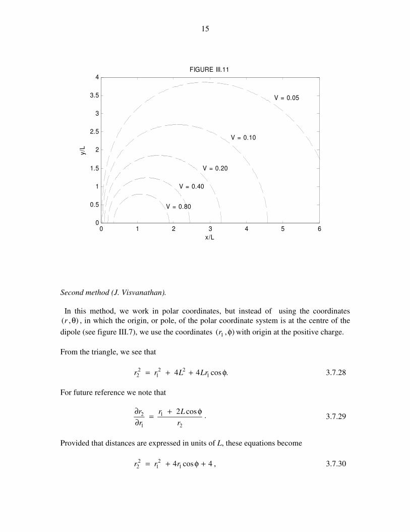
15

0 1 2 3 4 5 60

0.5

1

1.5

2

2.5

3

3.5

4

x/L

y/L

FIGURE III.11

V = 0.05

V = 0.10

V = 0.20

V = 0.40

V = 0.80

Second method (J. Visvanathan).

In this method, we work in polar coordinates, but instead of using the coordinates

),( θr , in which the origin, or pole, of the polar coordinate system is at the centre of the

dipole (see figure III.7), we use the coordinates ),( 1 φr with origin at the positive charge.

From the triangle, we see that

.cos44 122

12

2 φ++= LrLrr 3.7.28

For future reference we note that

.cos2

2

1

1

2

r

Lr

r

r φ+=

∂

∂ 3.7.29

Provided that distances are expressed in units of L, these equations become

4cos4 12

12

2 +φ+= rrr , 3.7.30

16

2

1

1

2 cos2

r

r

r

r φ+=

∂

∂. 3.7.31

If, in addition, electrical potential is expressed in units of L

Q

04πε, the potential at P is

given, as before (equation 3.17.15), by

.11

),(21

1rr

rV −=φ 3.7.32

Recall that r2 is given by equation 3.7.30, so that equation 3.7.32 is really an equation in

just V, r1 and φ.

In order to plot an equipotential, we fix some value of V; then we vary φ from 0 to π,

and, for each value of φ we have to try to calculate r1.This can be done by the Newton-

Raphson process, in which we make a guess at r1 and use the Newton-Raphson process to

obtain a better guess, and continue until successive guesses converge. It is best if we can

make a fairly good first guess, but the Newton-Raphson process will often converge very

rapidly even for a poor first guess.

Thus we have to solve the following equation for r1 for given values of V and φ,

011

)(21

1 =−−= Vrr

rf , 3.7.33

bearing in mind that r2 is given by equation 3.7.31.

By differentiation with respect to r1, we have

3

2

1

211

2

22

21

1

cos2111)('

r

r

rr

r

rr

rfφ+

+−=∂

∂+−= , 3.7.34

and we are all set to begin a Newton-Raphson iteration: './11 ffrr −= Having

obained r1, we can then obtain the ),( yx coordinates from φ+= cos1 1rx and

φ= sin1ry .

I tried this method and I got exactly the same result as by the first method and as shown

in figure III.11.

So which method do we prefer? Well, anyone who has worked through in detail the

derivations of equations 3.7.16 -3.7.27, and has then tried to program them for a

computer, will agree that the first method is very laborious and cumbersome. By

comparison Visvanathan’s method is much easier both to derive and to program. On the

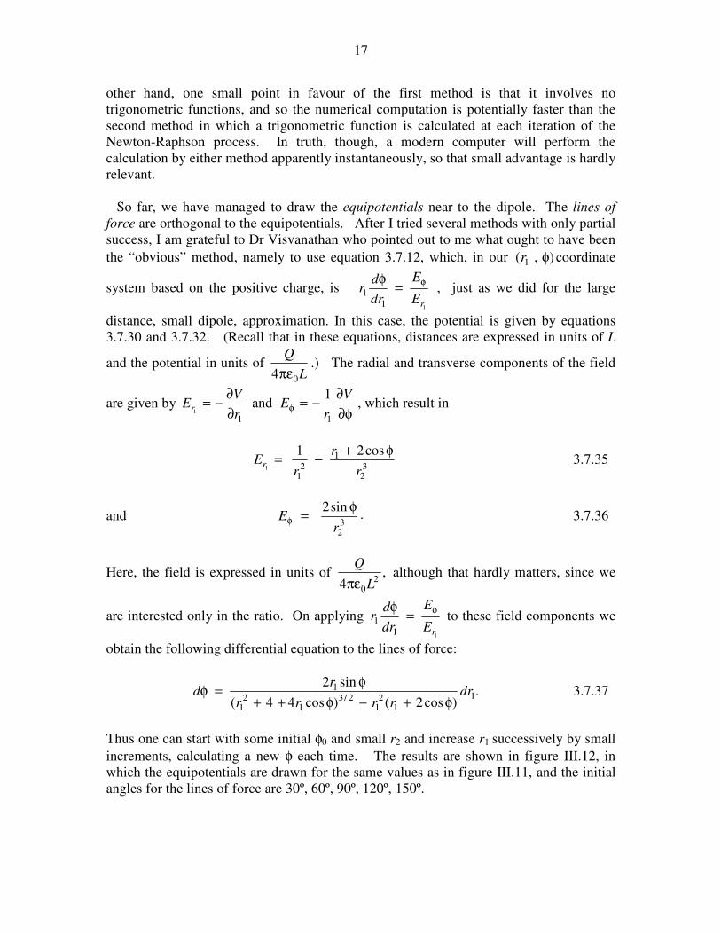
17

other hand, one small point in favour of the first method is that it involves no

trigonometric functions, and so the numerical computation is potentially faster than the

second method in which a trigonometric function is calculated at each iteration of the

Newton-Raphson process. In truth, though, a modern computer will perform the

calculation by either method apparently instantaneously, so that small advantage is hardly

relevant.

So far, we have managed to draw the equipotentials near to the dipole. The lines of

force are orthogonal to the equipotentials. After I tried several methods with only partial

success, I am grateful to Dr Visvanathan who pointed out to me what ought to have been

the “obvious” method, namely to use equation 3.7.12, which, in our ),( 1 φr coordinate

system based on the positive charge, is

11

1

rE

E

dr

dr

φ=

φ , just as we did for the large

distance, small dipole, approximation. In this case, the potential is given by equations

3.7.30 and 3.7.32. (Recall that in these equations, distances are expressed in units of L

and the potential in units of L

Q

04πε.) The radial and transverse components of the field

are given by φ∂

∂−=

∂

∂−= φ

V

rE

r

VE

r

11

1and

1, which result in

32

1

21

cos211

r

r

r

Er

φ+−= 3.7.35

and .sin2

32r

Eφ

=φ 3.7.36

Here, the field is expressed in units of ,4 2

0L

Q

πε although that hardly matters, since we

are interested only in the ratio. On applying

11

1

rE

E

dr

dr

φ=

φ to these field components we

obtain the following differential equation to the lines of force:

.)cos2()cos44(

sin21

12

12/3

12

1

1dr

rrrr

rd

φ+−φ++

φ=φ 3.7.37

Thus one can start with some initial φ0 and small r2 and increase r1 successively by small

increments, calculating a new φ each time. The results are shown in figure III.12, in

which the equipotentials are drawn for the same values as in figure III.11, and the initial

angles for the lines of force are 30º, 60º, 90º, 120º, 150º.

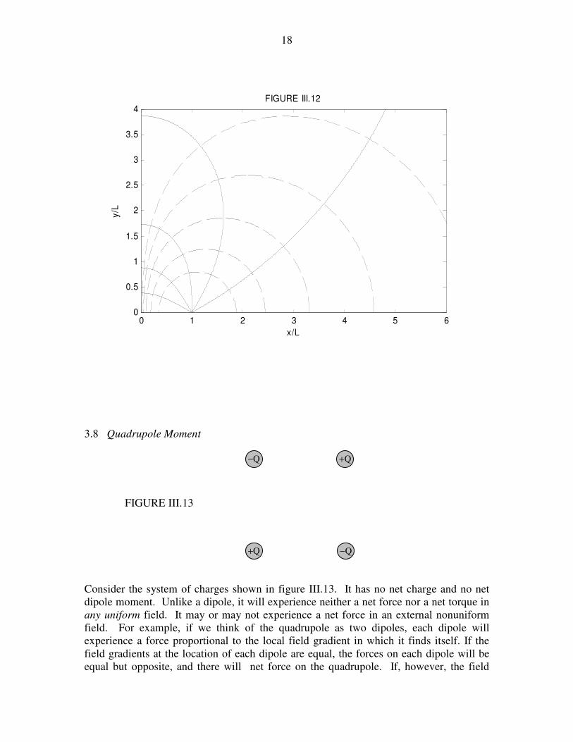
18

0 1 2 3 4 5 60

0.5

1

1.5

2

2.5

3

3.5

4

x/L

y/L

FIGURE III.12

3.8 Quadrupole Moment

Consider the system of charges shown in figure III.13. It has no net charge and no net

dipole moment. Unlike a dipole, it will experience neither a net force nor a net torque in

any uniform field. It may or may not experience a net force in an external nonuniform

field. For example, if we think of the quadrupole as two dipoles, each dipole will

experience a force proportional to the local field gradient in which it finds itself. If the

field gradients at the location of each dipole are equal, the forces on each dipole will be

equal but opposite, and there will net force on the quadrupole. If, however, the field

−Q

+Q

+Q

−Q

FIGURE III.13

19

gradients at the positions of the two dipoles are unequal, the forces on the two dipole will

be unequal, and there will be a net force on the quadruople. Thus there will be a net force

if there is a non-zero gradient of the field gradient. Stated another way, there will be no

net force on the quadrupole if the mixed second partial derivatives of the field componets

(the third derivatives of the potential!) are zero. Further, if the quadrupole is in a

nonuniform field, increasing, say, to the right, the upper pair will experience a force to

the right and the lower pair will experience a force to the left; thus the system will

experience a net torque in an inhomogeneous field, though there will be not net force

unless the field gradients on the two pairs are unequal.

The system possesses what is known as a quadrupole moment. While a single charge is

a scalar quantity, and a dipole moment is a vector quantity, the quadrupole moment is a

second order symmetric tensor.

The dipole moment of a system of charges is a vector with three components given by

.,,iiziiyiix

zQpyQpxQp ∑∑∑ === The quadrupole moment q has nine

components (of which six are distinct) defined by ,,2

iiixyiixxyxQqxQq ∑∑ == etc.,

and its matrix representation is

.

=

zzyzxz

yzyyxy

xzxyxx

qqq

qqq

qqq

q 3.8.1

For a continuous charge distribution with charge density ρ coulombs per square metre,

the components will be given by ,2 τρ= ∫ dxqxx

etc., where dτ is a volume element,

given in rectangular coordinates by dxdydz and in spherical coordinates by

.sin2 φθθ ddrdr The SI unit of quadrupole moment is C m2, and the dimensions are L

2Q,

By suitable rotation of axes, in the usual way (see for example section 2.17 of Classical

Mechanics), the matrix can be diagonalized, and the diagonal elements are then the

eigenvalues of the quadrupole moment, and the trace of the matrix is unaltered by the

rotation.

3.9 Potential at a Large Distance from a Charged Body

We wish to find the potential at a point P at a large distance R from a charged body, in

terms of its total charge and its dipole, quadrupole, and possibly higher-order moments.

There will be no loss of generality if we choose a set of axes such that P is on the z-axis.

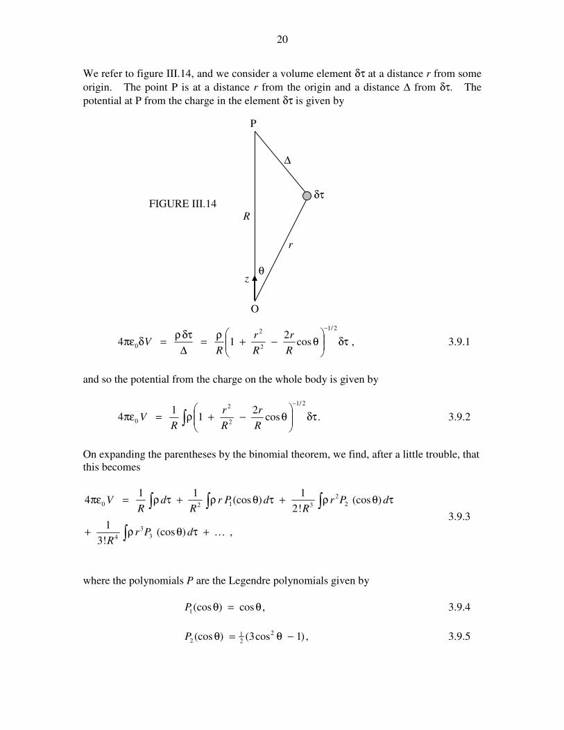
20

We refer to figure III.14, and we consider a volume element δτ at a distance r from some

origin. The point P is at a distance r from the origin and a distance ∆ from δτ. The

potential at P from the charge in the element δτ is given by

,cos2

14

2/1

2

2

0 δτ

θ−+

ρ=

∆

δτρ=δπε

−

R

r

R

r

RV 3.9.1

and so the potential from the charge on the whole body is given by

∫ δτ

θ−+ρ=πε

−

.cos2

11

4

2/1

2

2

0R

r

R

r

RV 3.9.2

On expanding the parentheses by the binomial theorem, we find, after a little trouble, that

this becomes

,)(cos!3

1

)(cos!2

1)(cos

114

3

3

4

2

2

3120

K+τθρ+

τθρ+τθρ+τρ=πε

∫

∫∫∫

dPrR

dPrR

dPrR

dR

V

3.9.3

where the polynomials P are the Legendre polynomials given by

,cos)(cos1 θ=θP 3.9.4

,)1cos3()(cos 2

21

2 −θ=θP 3.9.5

δτ

∆

R

θ

P

FIGURE III.14

O

r

z

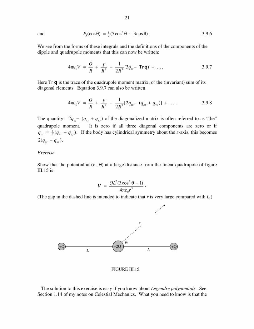
21

and .)cos3cos5()(cos 3

21

3 θ−θ=θP 3.9.6

We see from the forms of these integrals and the definitions of the components of the

dipole and quadrupole moments that this can now be written:

,)Tr3(2

14

320 K+−++=πε qzz

qRR

p

R

QV 3.9.7

Here Tr q is the trace of the quadrupole moment matrix, or the (invariant) sum of its

diagonal elements. Equation 3.9.7 can also be written

.)](2[2

14

320 K++−++=πεyyxxzz

qqqRR

p

R

QV 3.9.8

The quantity )(2yyxxzz

qqq +− of the diagonalized matrix is often referred to as “the”

quadrupole moment. It is zero if all three diagonal components are zero or if

.)(21

yyxxzzqqq += If the body has cylindrical symmetry about the z-axis, this becomes

.)(2xxzz

qq −

Exercise.

Show that the potential at (r , θ) at a large distance from the linear quadrupole of figure

III.15 is

.4

)1cos3(3

0

22

r

QLV

πε

−θ=

(The gap in the dashed line is intended to indicate that r is very large compared with L.)

The solution to this exercise is easy if you know about Legendre polynomials. See

Section 1.14 of my notes on Celestial Mechanics. What you need to know is that the

+Q +Q −2Q

•

r

θ

FIGURE III.15

L L

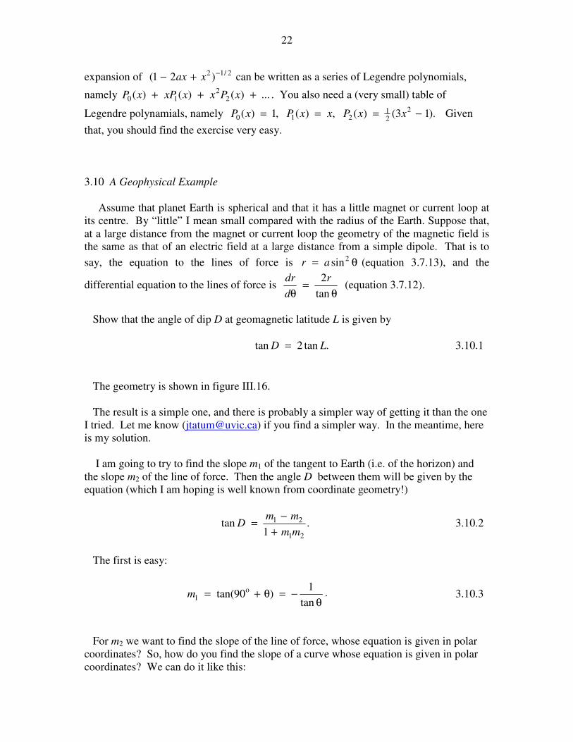
22

expansion of 2/12 )21( −+− xax can be written as a series of Legendre polynomials,

namely ...)()()( 22

10 +++ xPxxxPxP . You also need a (very small) table of

Legendre polynamials, namely ).13()(,)(,1)( 2

21

210 −=== xxPxxPxP Given

that, you should find the exercise very easy.

3.10 A Geophysical Example

Assume that planet Earth is spherical and that it has a little magnet or current loop at

its centre. By “little” I mean small compared with the radius of the Earth. Suppose that,

at a large distance from the magnet or current loop the geometry of the magnetic field is

the same as that of an electric field at a large distance from a simple dipole. That is to

say, the equation to the lines of force is θ= 2sinar (equation 3.7.13), and the

differential equation to the lines of force is θ

=θ tan

2r

d

dr (equation 3.7.12).

Show that the angle of dip D at geomagnetic latitude L is given by

.tan2tan LD = 3.10.1

The geometry is shown in figure III.16.

The result is a simple one, and there is probably a simpler way of getting it than the one

I tried. Let me know ([email protected]) if you find a simpler way. In the meantime, here

is my solution.

I am going to try to find the slope m1 of the tangent to Earth (i.e. of the horizon) and

the slope m2 of the line of force. Then the angle D between them will be given by the

equation (which I am hoping is well known from coordinate geometry!)

.1

tan21

21

mm

mmD

+

−= 3.10.2

The first is easy:

.tan

1)90tan( o

1θ

−=θ+=m 3.10.3

For m2 we want to find the slope of the line of force, whose equation is given in polar

coordinates? So, how do you find the slope of a curve whose equation is given in polar

coordinates? We can do it like this:

23

,cos θ= rx 3.10.4

,sin θ= ry 3.10.5

,sincos θθ−θ= drdrdx 3.10.6

.cossin θθ+θ= drdrdy 3.10.7

From these, we obtain

.sincos

cossin

θ−θ

θ+θ=

θ

θ

r

r

dx

dy

d

dr

d

dr

3.10.8

In our particular case, we have θ

=θ tan

2r

d

dr (equation 3.7.12), so if we substitute this

into equation 3.10.8 we soon obtain

.1cos3

cossin322

−θ

θθ=m 3.10.9

Now put equations 3.10.3 and 3.10.9 into equation 3.10.2, and, after a little algebra, we

soon obtain

.tan2tan

2tan LD =

θ= 3.10.10

24

Here is another question. The magnetic field is generally given the symbol B. Show that

the strength of the magnetic field )(LB at geomagnetic latitude L is given by

,sin31)0()( 2LBLB += 3.10.11

South North

Eq

uato

r

x

y

L

θ

D

m1

m2

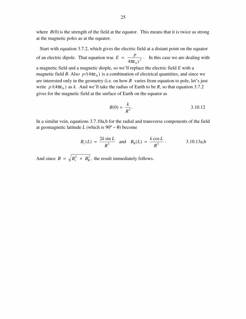
25

where )0(B is the strength of the field at the equator. This means that it is twice as strong

at the magnetic poles as at the equator.

Start with equation 3.7.2, which gives the electric field at a distant point on the equator

of an electric dipole. That equation was .4 3

0 y

pE

πε= In this case we are dealing with

a magnetic field and a magnetic diople, so we’ll replace the electric field E with a

magnetic field B. Also )4/( 0πεp is a combination of electrical quantities, and since we

are interested only in the geometry (i.e. on how B varies from equation to pole, let’s just

write )4/( 0πεp as k. And we’ll take the radius of Earth to be R, so that equation 3.7.2

gives for the magnetic field at the surface of Earth on the equator as

.)0(3

R

kB = 3.10.12

In a similar vein, equations 3.7.10a,b for the radial and transverse components of the field

at geomagnetic latitude L (which is 90º − θ) become

.cos

)(andsin2

)(33

R

LkLB

R

LkLB

r== θ 3.10.13a,b

And since ,22θ+= BBB

r the result immediately follows.

1

CHAPTER 4 BATTERIES, RESISTORS AND OHM’S LAW

4.1 Introduction An electric cell consists of two different metals, or carbon and a metal, called the poles, immersed or dipped into a liquid or some sort of a wet, conducting paste, known as the electrolyte, and, because of some chemical reaction between the two poles and the electrolyte, there exists a small potential difference (typically of the order of one or two volts) between the poles. This potential difference is much smaller than the hundreds or thousands of volts that may be obtained in typical laboratory experiments in electrostatics, and the electric field between the poles is also correspondingly small. Definition. The potential difference across the poles of a cell when no current is being taken from it is called the electromotive force (EMF) of the cell. The circuit symbol for a cell is drawn thus: The longer, thin line represents the positive pole and the shorter, thick line represents the negative pole. Several cells connected together form a battery of cells. Thus in principle a single cell should strictly be called just that – a cell – and the word battery should be restricted to a battery of several cells. However, in practice, most people use the word battery to mean either literally a battery of several cells, or a single cell. I shall not discuss in this chapter the detailed chemistry of why there exists such a potential difference, nor shall I discuss in detail the chemical processes that take place inside the several different varieties of cell. I shall just mention that in the cheaper types of flashlight battery (cell), the negative pole, made of zinc, is the outer casing of the cell, while the positive pole is a central carbon rod. The rather dirty mess that is the electrolyte is a mixture that is probably known only to the manufacturer, though it probably includes manganese oxide and ammonium chloride and perhaps such goo as flour or glue and goodness knows what else. Other types have a positive pole of nickelic hydroxide and a negative pole of cadmium metal in a potassium hydroxide electrolyte. A 12-volt car battery is typically a battery of 6 cells in series, in which the positive poles are lead oxide PbO2, the negative poles are metallic lead and the electrolyte is sulphuric acid. In some batteries, after they are exhausted, the poles are irreversibly damaged and the battery has to be discarded. In others, such as the nickel-cadmium or lead-acid cells, the chemical reaction is reversible, and so the cells can be recharged. I have heard the word “accumulator” used for a rechargeable battery, particularly the lead-acid car battery, but I don’t know how general that usage is.

2

Obviously the purpose of a battery is to extract a current from it. An electrolytic cell is quite the opposite. In an electrolytic cell, an electric current is forced into it from outside. This may be done in a laboratory, for example, to study the flow of electricity through an electrolyte, or in industrial processes such as electroplating. In an electrolytic cell, the current is forced into the cell by two electrodes, one of which (the anode) is maintained at a higher potential than the other (the cathode). The electrolyte contains positive ions (cations) and negative ions (anions), which can flow through the electrolyte. Naturally, the positive ions (cations) flow towards the negative electrode (the cathode) and the negative ions (the anions) flow towards the positive electrode (the anode). The direction of flow of electricity in an electrolytic cell is the opposite from the flow when a battery is being used to power an external circuit, and the roles of the two poles or electrodes are reversed. Thus some writers will refer to the positive pole of a battery as its “cathode”. It is not surprising therefore, that many a student (and, one might even guess, many a professor and textbook writer) has become confused over the words cathode and anode. The situation is not eased by referring to negatively charged electrons in a gaseous discharge tube as “cathode rays”. My recommendation would be: When referring to an electrolytic cell, use the word “electrodes”; when referring to a battery, use the word “poles”. Avoid the use of the prefixes “cat” and “an” altogether. Thus, refer to the positive and negative electrodes of an electrolytic cell, the positive and negative poles of a battery, and the positive and negative ions of an electrolyte. In that way your meaning will always be clear and unambiguous to yourself and to your audience or your readers. 4.2 Resistance and Ohm’s Law When a potential difference is maintained across the electrodes in an electrolytic cell, a current flows through the electrolyte. This current is carried by positive ions moving from the positive electrode towards the negative electrode and also, simultaneously, by negative ions moving from the negative electrode towards the positive electrode. The conventional direction of the flow of electricity is the direction in which positive charges are moving. That is to say, electricity flows from the positive electrode towards the negative electrode. The positive ions, then, are moving in the same direction as the conventional direction of flow of electricity, and the negative ions are moving in the opposite direction. When current flows in a metal, the current is carried exclusively by means of negatively charged electrons, and therefore the current is carried exclusively by means of particles that are moving in the opposite direction to the conventional flow of electricity. Thus “electricity” flows from a point of high potential to a point of lower potential; electrons move from a point of low potential to a point of higher potential.

3

When a potential difference V is applied across a resistor, the ratio of the potential difference across the resistor to the current I that flows through it is called the resistance, R, of the resistor. Thus .IRV = 4.2.1 This equation, which defines resistance, appears at first glance to say that the current through a resistor is proportional to the potential difference across it, and this is Ohm’s Law. Equation 4.2.1, however, implies a simple proportionality between V and I only if R is constant and independent of I or of V. In practice, when a current flows through a resistor, the resistor becomes hot, and its resistance increases – and then V and I are no longer linearly proportional to one another. Thus one would have to state Ohm’s Law in the form that the current through a resistor is proportional to the potential difference across it, provided that the temperature is held constant. Even so, there are some substances (and various electronic devices) in which the resistance is not independent of the applied potential difference even at constant temperature. Thus it is better to regard equation 4.2.1 as a definition of resistance rather than as a fundamental law, while also accepting that it is a good description of the behaviour of most real substances under a wide variety of conditions as long as the temperature is held constant. Definitions. If a current of one amp flows through a resistor when there is a potential difference of one volt across it, the resistance is one ohm (Ω). (Clear though this definition may appear, however, recall from chapter 1 that we have not yet defined exactly what we mean by an amp, nor a volt, so suddenly the meaning of “ohm” becomes a good deal less clear! I do promise a definition of “amp” in a later chapter – but in the meantime I crave your patience.)

The dimensions of resistance are .QTMLQT

QTML 2121

122−−

−

−−

=

The reciprocal of resistance is conductance, G. Thus I = GV. It is common informal practice to express conductance in “mhos”, a “mho” being an ohm−1. The official SI unit of conductance, however, is the siemens (S), which is the same thing as a “mho”, namely one A V−1. The resistance of a resistor is proportional to its length l and inversely proportional to its cross-sectional area A:

.AlR ρ

= 4.2.2

The constant of proportionality ρ is called the resistivity of the material of which the resistor is made. Its dimensions are ML3T−1Q−2, and its SI unit is ohm metre, or Ω m.

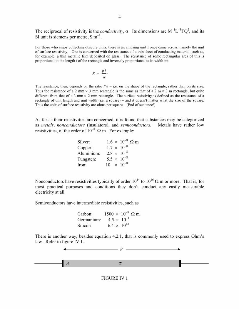
4

The reciprocal of resistivity is the conductivity, σ. Its dimensions are M−1L−3TQ2, and its SI unit is siemens per metre, S m−1. For those who enjoy collecting obscure units, there is an amusing unit I once came across, namely the unit of surface resistivity. One is concerned with the resistance of a thin sheet of conducting material, such as, for example, a thin metallic film deposited on glass. The resistance of some rectangular area of this is proportional to the length l of the rectangle and inversely proportional to its width w:

.w

lR

ρ=

The resistance, then, depends on the ratio l/w – i.e. on the shape of the rectangle, rather than on its size. Thus the resistance of a 2 mm × 3 mm rectangle is the same as that of a 2 m × 3 m rectangle, but quite different from that of a 3 mm × 2 mm rectangle. The surface resistivity is defined as the resistance of a rectangle of unit length and unit width (i.e. a square) – and it doesn’t matter what the size of the square. Thus the units of surface resistivity are ohms per square. (End of sentence!) As far as their resistivities are concerned, it is found that substances may be categorized as metals, nonconductors (insulators), and semiconductors. Metals have rather low resistivities, of the order of 10−8 Ω m. For example: Silver: 1.6 × 10−8 Ω m Copper: 1.7 × 10−8 Aluminium: 2.8 × 10−8 Tungsten: 5.5 × 10−8 Iron: 10 × 10−8 Nonconductors have resistivities typically of order 1014 to 1016 Ω m or more. That is, for most practical purposes and conditions they don’t conduct any easily measurable electricity at all. Semiconductors have intermediate resistivities, such as Carbon: 1500 × 10−8 Ω m Germanium: 4.5 × 10−1 Silicon 6.4 × 10+2 There is another way, besides equation 4.2.1, that is commonly used to express Ohm’s law. Refer to figure IV.1.

FIGURE IV.1

A

V

σ

5

We have a metal rod of length l, cross-sectional area A, electrical conductivity σ, and so its resistance is l/(σA). We clamp it between two points which have a potential difference of V between them, and consequently the magnitude of the electric field in the metal is E = V/l. Equation 4.2.1 (Ohm’s law) therefore becomes .)/( AlIlE σ= Now introduce

lIJ /= as the current density (amps per square metre). Them Ohm’s law becomes EJ σ= . This is usually written in vector form, since current and field are both vectors,

so that Ohm’s law is written .EJ σ= 4.2.3 4.3 Resistance and Temperature It is found that the resistivities of metals generally increase with increasing temperature, while the resistivities of semiconductors generally decrease with increasing temperature. It may be worth thinking a little about how electrons in a metal or semiconductor conduct electricity. In a solid metal, most of the electrons in an atom are used to form covalent bonds between adjacent atoms and hence to hold the solid together. But about one electron per atom is not tied up in this way, and these “conduction electrons” are more or less free to move around inside the metal much like the molecules in a gas. We can estimate roughly the speed at which the electrons are moving. Thus we recall the formula

mkT /3 for the root-mean-square speed of molecules in a gas, and maybe we can apply that to electrons in a metal just for a rough order of magnitude for their speed. Boltzmann’s constant k is about 1.38 × 10−23 J K−1 and the mass of the electron, m, is about 9.11 × 10−31 kg. If we assume that the temperature is about 27oC or 300 K, the root mean square electron speed would be about 1.2 × 105 m s−1. Now consider a current of 1 A flowing in a copper wire of diameter 1 mm – i.e. cross-sectional area 7.85 × 10−7 m2. The density of copper is 8.9 g cm−3, and its “atomic weight” (molar mass) is 63.5 g per mole, which means that there are 6.02 × 1023 (Avogadro’s number) of atoms in 63.5 grams, or 8.44 × 1022 atoms per cm3 or 8.44 × 1028 atoms per m3. If we assume that there is one conduction electron per atom, then there are 8.44 × 1028 conduction electrons per m3, or, in our wire of diameter 1 mm, 6.63 × 1022 conduction electrons per metre. The speed at which the electrons are carrying the current of one amp is the current divided by the charge per unit length, and with the charge on a single electron being 1.60 × 10−19 C, we find that the speed at which the electrons are carrying the current is about 9.4 × 10−5 m s−1. Thus we have this picture of electrons moving in random directions at a speed of about 1.2 × 105 m s−1 (the thermal motion) and, superimposed on that, a very slow drift speed of only 9.4 × 10−5 m s−1 for the electron current. If you were able to see the electrons, you

6

would see them dashing hither and thither at very high speeds, but you wouldn’t even notice the very slow drift in the direction of the current. When you connect a long wire to a battery, however, the current (the slow electron drift) starts almost instantaneously along the entire length of the wire. If the electrons were in a complete vacuum, rather than in the interior of a metal, they would accelerate as long as they were in an electron field. The electrons inside the metal also accelerate, but they are repeatedly stopped in their tracks by collisions with the metal atoms – and then they start up again. If the temperature is increased, the vibrations of the atoms within the metal lattice increase, and this presumably somehow increases the resistance to the electron flow, or decreases the mean time or the mean path-length between collisions. In a semiconductor, most of the electrons are required for valence bonding between the atoms – but there are a few (much fewer than one per atom) free, conduction electrons. As the temperature is increased, more electrons are shaken free from their valence duties, and they then take on the task of conducting electricity. Thus the conductivity of a semiconductor increases with increasing temperature. The temperature coefficient of resistance, α, of a metal (or other substance) is the fractional increase in its resistivity per unit rise in temperature:

.1Td

d ρρ

=α 4.3.1

In SI units it would be expressed in K−1. However, in many practical applications the temperature coefficient is defined in relation to the change in resistance compared with the resistivity at a temperature of 20oC, and is given by the equation ,)]20(1[20 −α+ρ=ρ t 4.3.2 where t is the temperature in degrees Celsius. Examples: Silver: 3.8 × 10−3 C o −1 Copper: 3.9 × 10−3 Aluminium: 3.9 × 10−3 Tungsten: 4.5 × 10−3 Iron: 5.0 × 10−3 Carbon: −0.5 × 10−3 C o −1 Germanium: −48 × 10−3 Silicon −75 × 10−3 Some metallic alloys with commercial names such as nichrome, manganin, constantan, eureka, etc., have fairly large resistivities and very low temperature coefficients.

7

As a matter of style, note that the kelvin is a unit of temperature, much a the metre is a unit of length. Thus, when discussing temperatures, there is no need to use the “degree” symbol with the kelvin. When you are talking about some other temperature scale, such as Celsius, one needs to say “20 degrees on the Celsius scale” – thus 20oC. But when one is talking about a temperature interval of so many Celsius degrees, this is written Co. I have adhered to this convention above. The resistivity of platinum as a function of temperature is used as the basis of the platinum resistance thermometer, useful under conditions and temperatures where other types of thermometers may not be useful, and it is also used for defining a practical temperature scale at high temperatures. A bolometer is an instrument used for detecting and measuring infrared radiation. The radiation is focussed on a blackened platinum disc, which consequently rises in temperature. The temperature rise is measured by measuring the increase in resistance. A thermistor is a semiconducting device whose resistance is very sensitive to temperature, and it can be used for measuring or controlling temperature. 4.4 Resistors in Series .321 RRRR ++= 4.4.1 The current is the same in each. The potential difference is greatest across the largest resistance. 4.5 Conductors in Parallel .321 GGGG ++= 4.5.1

R1 R2 R3

FIGURE IV.2

FIGURE IV.3

G1

G2

G3

8

That is to say .1111

321 RRRR++= 4.5.2

The potential difference is the same across each. The current is greatest through the largest conductance – i.e. through the smallest resistance. 4.6 Dissipation of Energy When current flows through a resistor, electricity is falling through a potential difference. When a coulomb drops through a volt, it loses potential energy 1 joule. This energy is dissipated as heat. When a current of I coulombs per second falls through a potential difference of V volts, the rate of dissipation of energy is IV, which can also be written (by making use of Ohm’s law) ./or 22 RVRI If two resistors are connected in series, the current is the same in each, and we see from the formula RI 2 that more heat is generated in the larger resistance. If two resistors are connected in parallel, the potential difference is the same across each, and we see from the formula RV /2 that more heat is generated in the small resistance. 4.7 Electromotive Force and Internal Resistance The reader is reminded of the following definition from section 4.1:

Definition. The potential difference across the poles of a cell when no current is being taken from it is called the electromotive force (EMF) of the cell. I shall use the symbol E for EMF. Question. A 4 Ω resistance is connected across a cell of EMF 2 V. What current flows? The immediate answer is 0.5 A – but this is likely to be wrong. The reason is that a cell has a resistance of its own – its internal resistance. The internal resistance of a lead-acid cell is typically quite small, but most dry cells have an appreciable internal resistance. If the external resistance is R and the internal resistance is r, the total resistance of the circuit is R + r, so that the current that flows is E /(R + r). Whenever a current is taken from a cell (or battery) the potential difference across its poles drops to a value less than its EMF. We can think of a cell as an EMF in series with an internal resistance:

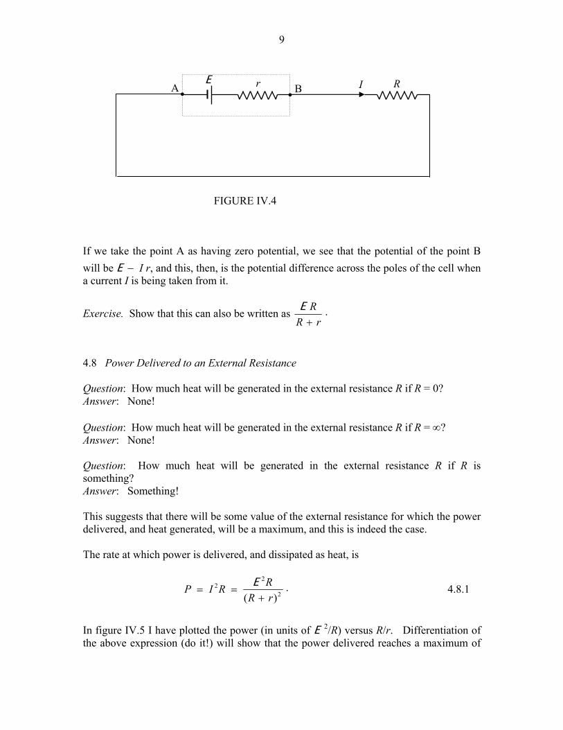
9

If we take the point A as having zero potential, we see that the potential of the point B will be E − I r, and this, then, is the potential difference across the poles of the cell when a current I is being taken from it.

Exercise. Show that this can also be written as .rR

R+

E

4.8 Power Delivered to an External Resistance Question: How much heat will be generated in the external resistance R if R = 0? Answer: None! Question: How much heat will be generated in the external resistance R if R = ∞? Answer: None! Question: How much heat will be generated in the external resistance R if R is something? Answer: Something! This suggests that there will be some value of the external resistance for which the power delivered, and heat generated, will be a maximum, and this is indeed the case. The rate at which power is delivered, and dissipated as heat, is

.)( 2

22

rRRRIP

+==

E 4.8.1

In figure IV.5 I have plotted the power (in units of E 2/R) versus R/r. Differentiation of the above expression (do it!) will show that the power delivered reaches a maximum of

•• A

FIGURE IV.4

B R I E r

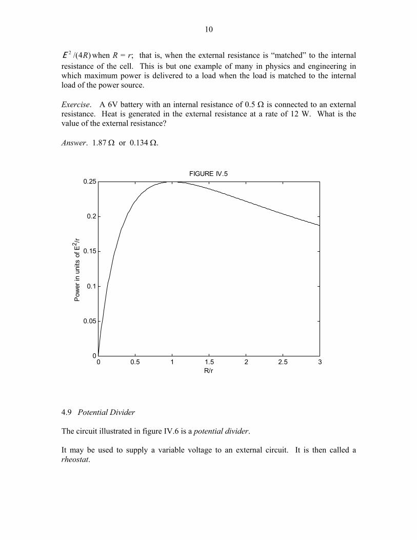
10

)4/(2 RE when R = r; that is, when the external resistance is “matched” to the internal resistance of the cell. This is but one example of many in physics and engineering in which maximum power is delivered to a load when the load is matched to the internal load of the power source. Exercise. A 6V battery with an internal resistance of 0.5 Ω is connected to an external resistance. Heat is generated in the external resistance at a rate of 12 W. What is the value of the external resistance? Answer. 1.87 Ω or 0.134 Ω.

0 0.5 1 1.5 2 2.5 30

0.05

0.1

0.15

0.2

0.25

R/r

Pow

er in

uni

ts o

f E2 /r

FIGURE IV.5

4.9 Potential Divider The circuit illustrated in figure IV.6 is a potential divider. It may be used to supply a variable voltage to an external circuit. It is then called a rheostat.

11

Or it may be used to compare potential differences, in which case it is called a potentiometer. (In practice many people refer to such a device as a “pot”, regardless of the use to which it is put.) For example, in figure IV.7, a balance point (no current in the ammeter, A) is found when the potential drop down the length x of the resistance wire is equal to the EMF of the small cell. (Note that, since no current is being taken from the small cell, the potential difference across its poles is indeed the EMF.) One could compare the EMFs of two cells in this manner, one of which might be a “standard cell” whose EMF is known. In figure IV.8, a current is flowing through a resistor (which is assumed to be in part of some external circuit, not drawn), and, assuming that the potential gradient down the potentiometer has been calibrated with a standard cell, the potentiometer is being used to measure the potential difference across the resistor. That is, the potentiometer is being used as a voltmeter.

• •

FIGURE IV.6

• •

FIGURE IV.7

A

x

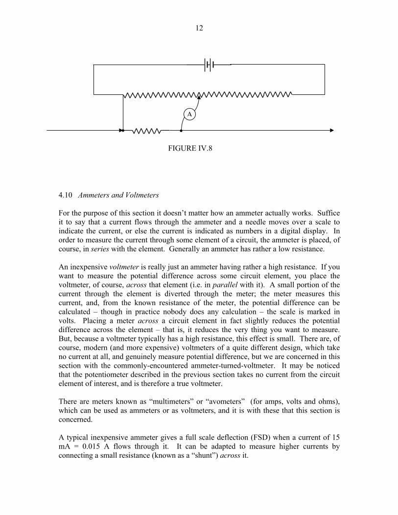
12

4.10 Ammeters and Voltmeters For the purpose of this section it doesn’t matter how an ammeter actually works. Suffice it to say that a current flows through the ammeter and a needle moves over a scale to indicate the current, or else the current is indicated as numbers in a digital display. In order to measure the current through some element of a circuit, the ammeter is placed, of course, in series with the element. Generally an ammeter has rather a low resistance. An inexpensive voltmeter is really just an ammeter having rather a high resistance. If you want to measure the potential difference across some circuit element, you place the voltmeter, of course, across that element (i.e. in parallel with it). A small portion of the current through the element is diverted through the meter; the meter measures this current, and, from the known resistance of the meter, the potential difference can be calculated – though in practice nobody does any calculation – the scale is marked in volts. Placing a meter across a circuit element in fact slightly reduces the potential difference across the element – that is, it reduces the very thing you want to measure. But, because a voltmeter typically has a high resistance, this effect is small. There are, of course, modern (and more expensive) voltmeters of a quite different design, which take no current at all, and genuinely measure potential difference, but we are concerned in this section with the commonly-encountered ammeter-turned-voltmeter. It may be noticed that the potentiometer described in the previous section takes no current from the circuit element of interest, and is therefore a true voltmeter. There are meters known as “multimeters” or “avometers” (for amps, volts and ohms), which can be used as ammeters or as voltmeters, and it is with these that this section is concerned. A typical inexpensive ammeter gives a full scale deflection (FSD) when a current of 15 mA = 0.015 A flows through it. It can be adapted to measure higher currents by connecting a small resistance (known as a “shunt”) across it.

• •

FIGURE IV.8

A

13

Let’s suppose, for example, that we have a meter that which shows a FSD when a current of 0.015 A flows through it, and that the resistance of the meter is 10 Ω. We would like to use the meter to measure currents as high as 0.15 A. What value of shunt resistance shall we put across the meter? Well, when the total current is 0.15 A, we want 0.015 A to flow through the meter (which then shows FSD) and the remainder, 0.135 A, is to flow through the shunt. With a current of 0.015 A flowing through the 10 Ω meter, the potential difference across it is 0.15 V. This is also the potential difference across the shunt, and, since the current through the shunt is 0.135 A, the resistance of the shunt must be 1.11 Ω. We can also use the meter as a voltmeter. Suppose, for example, that we want to measure voltages (horrible word!) of up to 1.5 V. We place a large resistance R in series with the meter, and then place the meter-plus-series-resistance across the potential difference to measured. The total resistance of meter-plus-series-resistance is (10 + R), and it will show a FSD when the current through it is 0.015 A. We want this to happen when the potential difference across it is 1.5 volts. This 1.5 = 0.015 × (10 + R), and so R = 90 Ω. 4.11 Wheatstone Bridge

G

R1 R2

R3 R4

FIGURE IV.9

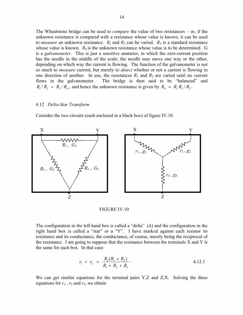
14

The Wheatstone bridge can be used to compare the value of two resistances – or, if the unknown resistance is compared with a resistance whose value is known, it can be used to measure an unknown resistance. R1 and R2 can be varied. R3 is a standard resistance whose value is known. R4 is the unknown resistance whose value is to be determined. G is a galvanometer. This is just a sensitive ammeter, in which the zero-current position has the needle in the middle of the scale; the needle may move one way or the other, depending on which way the current is flowing. The function of the galvanometer is not so much to measure current, but merely to detect whether or not a current is flowing in one direction of another. In use, the resistances R1 and R2 are varied until no current flows in the galvanometer. The bridge is then said to be “balanced” and

,// 4321 RRRR = and hence the unknown resistance is given by ./ 2314 RRRR = 4.12 Delta-Star Transform Consider the two circuits (each enclosed in a black box) of figure IV.10. The configuration in the left hand box is called a “delta” (∆) and the configuration in the right hand box is called a “star” or a “Y”. I have marked against each resistor its resistance and its conductance, the conductance, of course, merely being the reciprocal of the resistance. I am going to suppose that the resistance between the terminals X and Y is the same for each box. In that case:

.)(

321

21321 RRR

RRRrr++

+=+ 4.12.1

We can get similar equations for the terminal pairs Y,Z and Z,X. Solving the three equations for r1 , r2 and r3, we obtain

X

Z

R1 , G1

R3 , G3

R2 , G2

• •

•

Y X

Z

• •

•

Y

r1 , g1 r2 , g2

r3 , g3

FIGURE IV.10

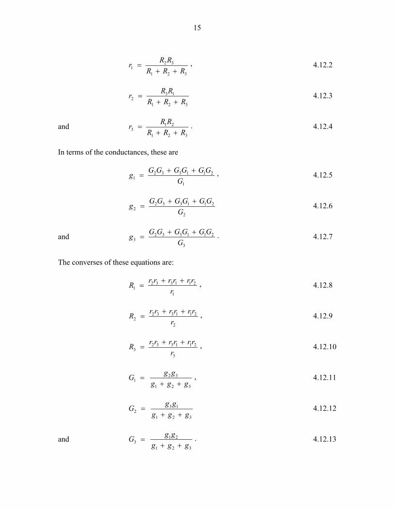
15

,321

321 RRR

RRr++

= 4.12.2

321

132 RRR

RRr++

= 4.12.3

and .321

213 RRR

RRr++

= 4.12.4

In terms of the conductances, these are

,1

2113321 G

GGGGGGg ++= 4.12.5

2

2113322 G

GGGGGGg ++= 4.12.6

and .3

2113323 G

GGGGGGg ++= 4.12.7

The converses of these equations are:

,1

2113321 r

rrrrrrR ++= 4.12.8

,2

2113322 r

rrrrrrR ++= 4.12.9

,3

2113323 r

rrrrrrR ++= 4.12.10

,321

321 ggg

ggG++

= 4.12.11

321

132 ggg

ggG++

= 4.12.12

and .321

213 ggg

ggG++

= 4.12.13

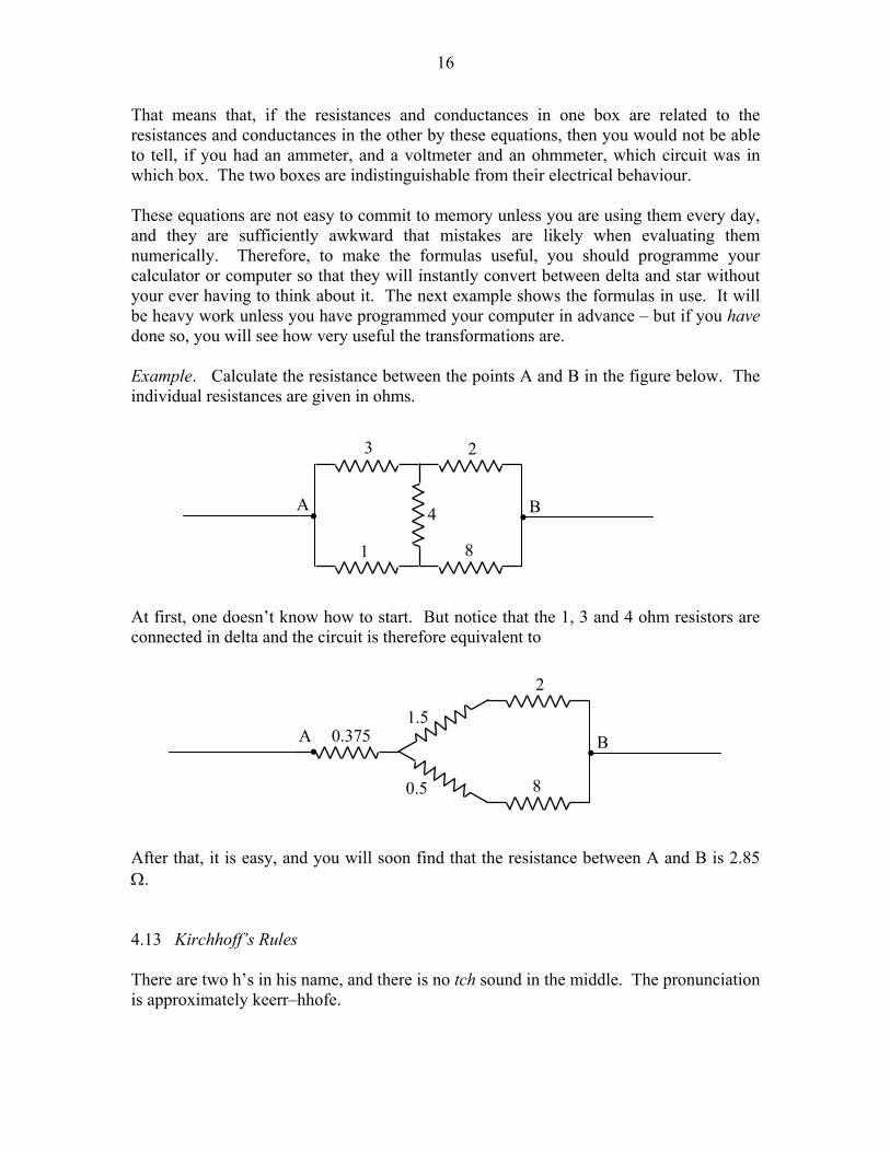
16

That means that, if the resistances and conductances in one box are related to the resistances and conductances in the other by these equations, then you would not be able to tell, if you had an ammeter, and a voltmeter and an ohmmeter, which circuit was in which box. The two boxes are indistinguishable from their electrical behaviour. These equations are not easy to commit to memory unless you are using them every day, and they are sufficiently awkward that mistakes are likely when evaluating them numerically. Therefore, to make the formulas useful, you should programme your calculator or computer so that they will instantly convert between delta and star without your ever having to think about it. The next example shows the formulas in use. It will be heavy work unless you have programmed your computer in advance – but if you have done so, you will see how very useful the transformations are. Example. Calculate the resistance between the points A and B in the figure below. The individual resistances are given in ohms. At first, one doesn’t know how to start. But notice that the 1, 3 and 4 ohm resistors are connected in delta and the circuit is therefore equivalent to After that, it is easy, and you will soon find that the resistance between A and B is 2.85 Ω. 4.13 Kirchhoff’s Rules There are two h’s in his name, and there is no tch sound in the middle. The pronunciation is approximately keerr–hhofe.

1 8

• •

3

4

2

A B

8

•

2

B • A 0.375

1.5

0.5

17

The rules themselves are simple and are self-evident. What has to be learned, however, is the art of using them. K1: The net current going into any point in a circuit is zero; expressed otherwise, the sum of all the currents entering any point in a circuit is equal to the sum of all the currents leaving the point. K2: The sum of all the EMFs and IR products in a closed circuit is zero. Expressed otherwise, as you move around a closed circuit, the potential will sometimes rise and sometimes fall as you encounter a battery or a resistance; but, when you come round again to the point where you started, there is no change in potential. Example. In the above circuit, the 24 V battery is assumed to have negligible internal resistance. Calculate the current in each of the resistors. The art of applying Kirchhoff’s rules is as follows. 1. Draw a large circuit diagram in pencil. 2. Count the number of independent resistors. (Two is series with nothing in between don’t count as independent.) This tells you how many independent equations you can obtain, and how many unknowns you can solve for. In this case, there are five independent resistors; you can get five independent equations and you can solve for five unknowns. 3. Mark in the unknown currents. If you don’t know the directions of some of them, don’t spend time trying to think it out. Just make a wild guess. If you are wrong, you will merely get a negative answer for it. Those who have some physical insight might already guess (correctly) that I have marked I5 in the wrong direction, but that doesn’t matter.

1 8

• •

3

4

2

A B

24 V

I4

I5

Ω

I1

I2

I3 Ω

Ω

Ω

Ω

C

D

O

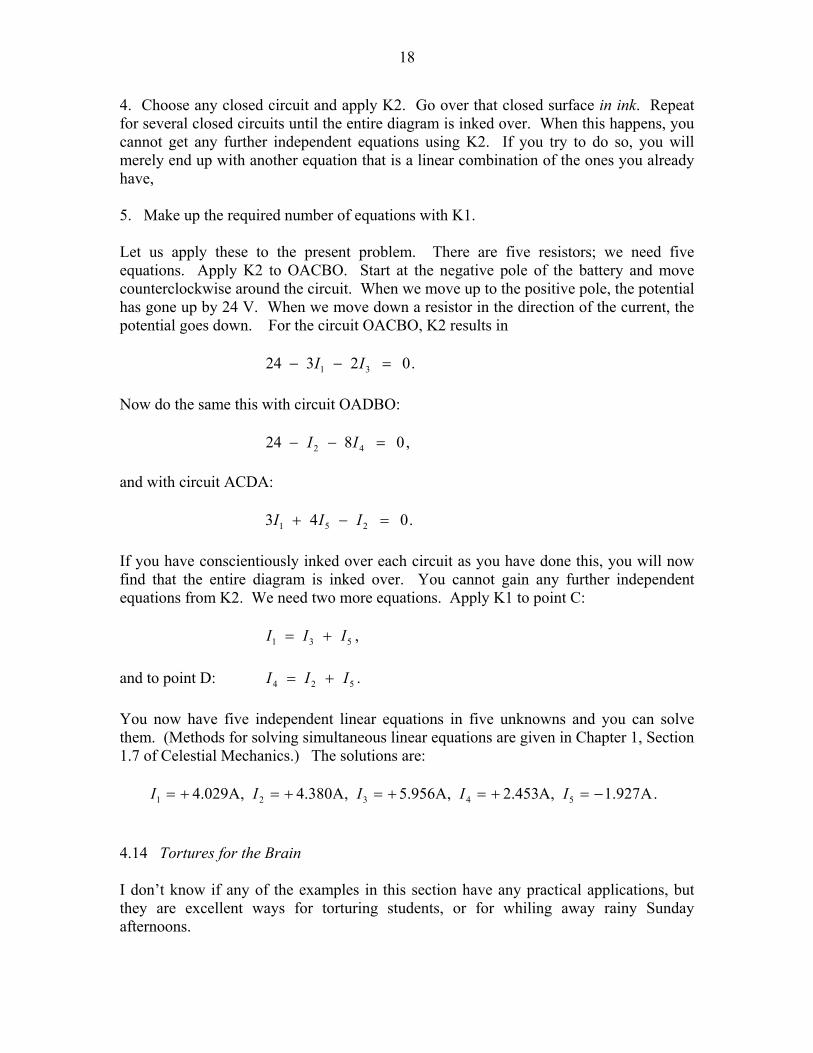
18

4. Choose any closed circuit and apply K2. Go over that closed surface in ink. Repeat for several closed circuits until the entire diagram is inked over. When this happens, you cannot get any further independent equations using K2. If you try to do so, you will merely end up with another equation that is a linear combination of the ones you already have, 5. Make up the required number of equations with K1. Let us apply these to the present problem. There are five resistors; we need five equations. Apply K2 to OACBO. Start at the negative pole of the battery and move counterclockwise around the circuit. When we move up to the positive pole, the potential has gone up by 24 V. When we move down a resistor in the direction of the current, the potential goes down. For the circuit OACBO, K2 results in .02324 31 =−− II Now do the same this with circuit OADBO: ,0824 42 =−− II and with circuit ACDA: .043 251 =−+ III If you have conscientiously inked over each circuit as you have done this, you will now find that the entire diagram is inked over. You cannot gain any further independent equations from K2. We need two more equations. Apply K1 to point C: ,531 III += and to point D: .524 III += You now have five independent linear equations in five unknowns and you can solve them. (Methods for solving simultaneous linear equations are given in Chapter 1, Section 1.7 of Celestial Mechanics.) The solutions are: .A927.1,A453.2,A956.5,A380.4,A029.4 54321 −=+=+=+=+= IIIII 4.14 Tortures for the Brain I don’t know if any of the examples in this section have any practical applications, but they are excellent ways for torturing students, or for whiling away rainy Sunday afternoons.

19

4.14.1 The drawing shows 12 resistances, each of value r Ω, arranged along the edges of a cube. What is the resistance across opposite corners of the cube? 4.14.2

12 V

A

B

20

The drawing shows six resistors, each of resistance 1 Ω, arranged along the edges of a tetrahedron. A 12 V battery is connected across one of the resistors. Calculate the current between points A and B. 4.14.3 The figure shows six resistors, whose resistances in ohms are marked, arranged along the edges of a tetrahedron. Calculate the net resistance between C and D. 4.14.4 R1 = 8 Ω and R2 = 0.5 Ω are connected across a battery. The rate at which heat is generated is the same whether they are connected in series or in parallel. What is the internal resistance r of the battery? 4.14.5 R1 = 0.25 Ω and R2 = ? are connected across a battery whose internal resistance r is 0.5 Ω. The rate at which heat is generated is the same whether they are connected in series or in parallel. What is the value of R2?

6

2

12 4

3

D C

5

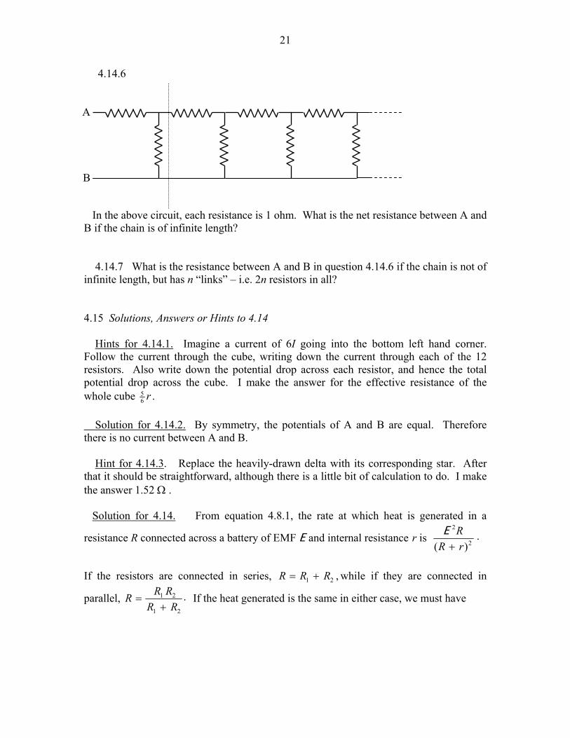
21

4.14.6 In the above circuit, each resistance is 1 ohm. What is the net resistance between A and B if the chain is of infinite length? 4.14.7 What is the resistance between A and B in question 4.14.6 if the chain is not of infinite length, but has n “links” – i.e. 2n resistors in all? 4.15 Solutions, Answers or Hints to 4.14 Hints for 4.14.1. Imagine a current of 6I going into the bottom left hand corner. Follow the current through the cube, writing down the current through each of the 12 resistors. Also write down the potential drop across each resistor, and hence the total potential drop across the cube. I make the answer for the effective resistance of the whole cube .6

5 r Solution for 4.14.2. By symmetry, the potentials of A and B are equal. Therefore there is no current between A and B. Hint for 4.14.3. Replace the heavily-drawn delta with its corresponding star. After that it should be straightforward, although there is a little bit of calculation to do. I make the answer 1.52 Ω . Solution for 4.14. From equation 4.8.1, the rate at which heat is generated in a

resistance R connected across a battery of EMF E and internal resistance r is .)( 2

2

rRR

+E

If the resistors are connected in series, ,21 RRR += while if they are connected in

parallel, .21

21

RRRRR

+= If the heat generated is the same in either case, we must have

A

B

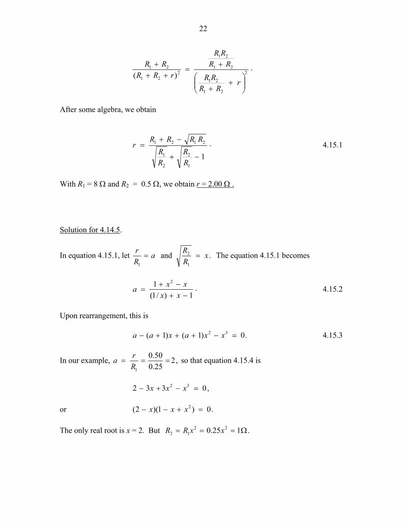
22

.)( 2

21

21

21

21

221

21

+

+

+=

+++

rRR

RR

RRRR

rRRRR

After some algebra, we obtain

.

11

2

2

1

2121

−+

−+=

RR

RR

RRRRr 4.15.1

With R1 = 8 Ω and R2 = 0.5 Ω, we obtain r = 2.00 Ω . Solution for 4.14.5.

In equation 4.15.1, let .and1

2

1

xRRa

Rr

== The equation 4.15.1 becomes

.1)/1(

1 2

−+−+

=xx

xxa 4.15.2

Upon rearrangement, this is .0)1()1( 32 =−+++− xxaxaa 4.15.3

In our example, ,225.050.0

1

===Rra so that equation 4.15.4 is

,0332 32 =−+− xxx or .0)1)(2( 2 =+−− xxx The only real root is x = 2. But .125.0 22

12 Ω=== xxRR

23

Solution to 4.14.6 Suppose that there are n links (2n resistors) to the right of the dotted line, and that the effective resistance of these n links is Rn. Add one more link, to the left. The effective resistance of the n + 1 links is then

.112

1 ++

=+n

nn R

RR 4.15.4

As ., 1 RRRn nn →→∞→ + .01or,112 2 =−−

++

=∴ RRRRR

Whence, .989033618.1)15(2

1 Ω=+=R Solution to 4.14.7 By repeated application of equation 4.15.4, we find:

989033618.112990033618.111999033618.110056034618.19448034618.18135037618.17556055618.16818181618.15619047619.14000000625.13667666666.12

21

4636875025

17711286576765

1094625844181

9871597

377610144233

55892134

81335

=

=

=

=

=

=

=

=

=

=

=

nRn

Inspection shows that ,2

12

n

nn F

FR += where Fm is the mth member of the Fibonacci

sequence: 1 1 2 3 5 8 13 21 ...... But, from the theory of Fibonacci sequences,

.2

512

515

1

−−

+=

mm

mF

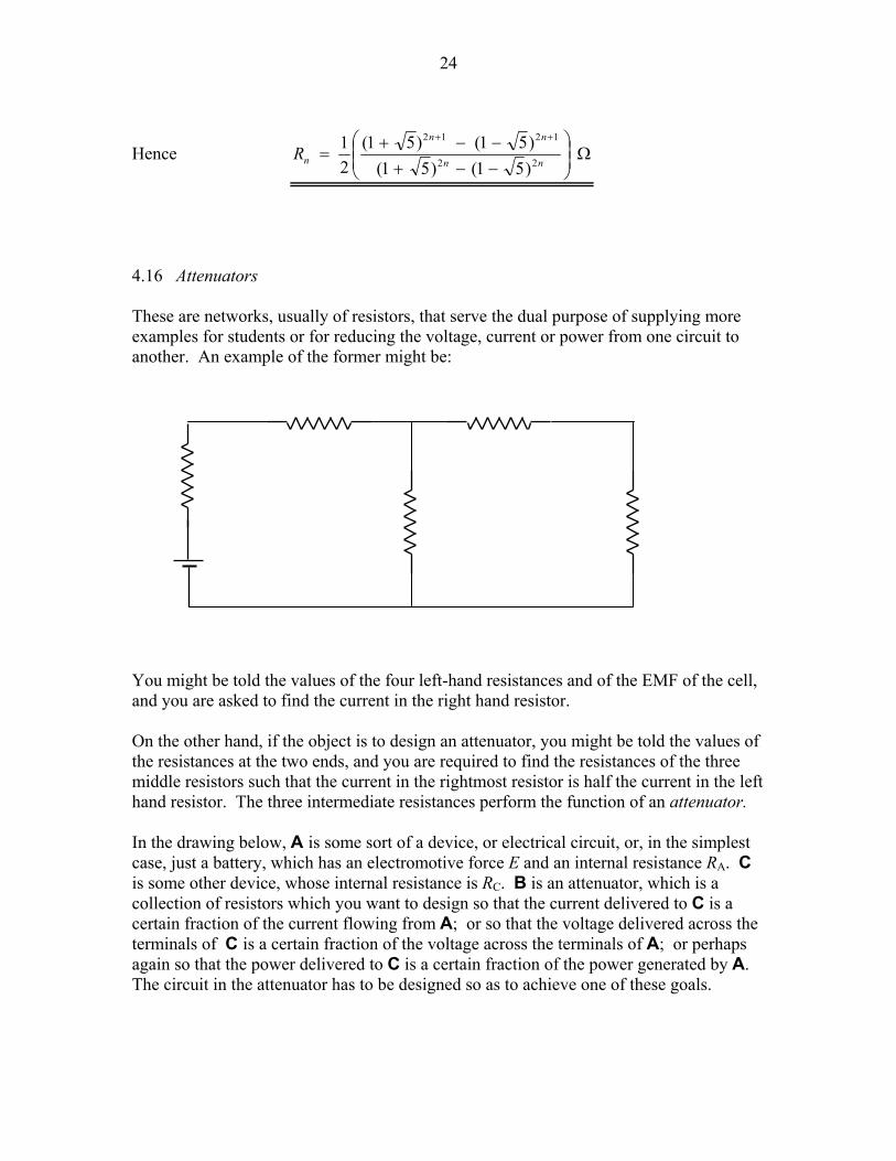
24

Hence Ω

−−+−−+

=++

nn

nn

nR22

1212

)51()51()51()51(

21

4.16 Attenuators These are networks, usually of resistors, that serve the dual purpose of supplying more examples for students or for reducing the voltage, current or power from one circuit to another. An example of the former might be: You might be told the values of the four left-hand resistances and of the EMF of the cell, and you are asked to find the current in the right hand resistor. On the other hand, if the object is to design an attenuator, you might be told the values of the resistances at the two ends, and you are required to find the resistances of the three middle resistors such that the current in the rightmost resistor is half the current in the left hand resistor. The three intermediate resistances perform the function of an attenuator. In the drawing below, A is some sort of a device, or electrical circuit, or, in the simplest case, just a battery, which has an electromotive force E and an internal resistance RA. C is some other device, whose internal resistance is RC. B is an attenuator, which is a collection of resistors which you want to design so that the current delivered to C is a certain fraction of the current flowing from A; or so that the voltage delivered across the terminals of C is a certain fraction of the voltage across the terminals of A; or perhaps again so that the power delivered to C is a certain fraction of the power generated by A. The circuit in the attenuator has to be designed so as to achieve one of these goals.

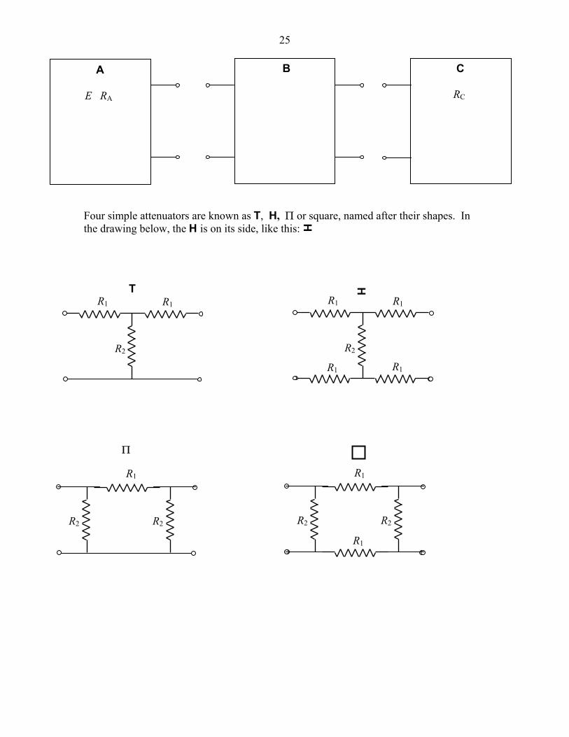
25

Four simple attenuators are known as T, H, Π or square, named after their shapes. In the drawing below, the H is on its side, like this:

A E RA

C RC

B

H

R1 R1

R2

T R1 R1

R2

H

R1 R1

R1

R2

Π

R2

R1

R2 R2

R1

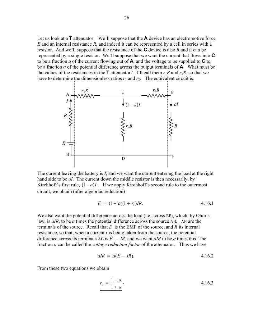
26

Let us look at a T attenuator. We’ll suppose that the A device has an electromotive force E and an internal resistance R, and indeed it can be represented by a cell in series with a resistor. And we’ll suppose that the resistance of the C device is also R and it can be represented by a single resistor. We’ll suppose that we want the current that flows into C to be a fraction a of the current flowing out of A, and the voltage to be supplied to C to be a fraction a of the potential difference across the output terminals of A. What must be the values of the resistances in the T attenuator? I’ll call them r1R and r2R, so that we have to determine the dimensionless ratios r1 and r2. The equivalent circuit is: The current leaving the battery is I, and we want the current entering the load at the right hand side to be aI. The current down the middle resistor is then necessarily, by Kirchhoff’s first rule, Ia)1( − . If we apply Kirchhoff’s second rule to the outermost circuit, we obtain (after algebraic reduction)

.)1)(1( 1 IRraE ++= 4.16.1

We also want the potential difference across the load (i.e. across EF), which, by Ohm’s law, is aIR, to be a times the potential difference across the source AB. AB are the terminals of the source. Recall that E is the EMF of the source, and R its internal resistance, so that, when a current I is being taken from the source, the potential difference across its terminals AB is E − IR, and we want aIR to be a times this. The fraction a can be called the voltage reduction factor of the attenuator. Thus we have ).( IREaaIR −= 4.16.2 From these two equations we obtain

.11

1 aar

+−

= 4.16.3

E

R

R

r1R

r2R

r1R

aI Ia)1( − I A

B

C

D

E

F

27

Application of Kirchhoff’s second rule to the right hand circuit gives

,)1()1( 12 IRraIRar +=− 4.16.4

which, in combination with equation 4.16.3, yields

.1

222 a

ar−

= 4.16.5

Thus, if source and load resistance are each equal to R, and we want a voltage reduction factor of 2

1 , we must choose r1R to be R31 , and r2R to be R3

4 . You might like to try the same problem for the , Π and square attenuators. I am not absolutely certain (I haven’t checked them carefully), but I believe the answers are: For :

+−

=aar

11

21

1 22 12

aar

−= 4.16.6

For Π :

aar

21 2

1−

= aar

−+

=11

2 4.16.7

For square :

−=

aar

21

21 2

1 aar

−+

=11

2 4.16.7

H

H

1

CHAPTER 5 CAPACITORS

5.1 Introduction A capacitor consists of two metal plates separated by a nonconducting medium (known as the dielectric medium or simply the dielectric, or by a vacuum. It is represented by the electrical symbol . Capacitors of one sort or another are included in almost any electronic device. Physically, there is a vast variety of shapes, sizes and construction, depending upon their particular application. This chapter, however, is not primarily concerned with real, practical capacitors and how they are made and what they are used for, although a brief section at the end of the chapter will discuss this. In addition to their practical uses in electronic circuits, capacitors are very useful to professors for torturing students during exams, and, more importantly, for helping students to understand the concepts of and the relationships between electric fields E and D, potential difference, permittivity, energy, and so on. The capacitors in this chapter are, for the most part, imaginary academic concepts useful largely for pedagogical purposes. Need the electronics technician or electronics engineer spend time on these academic capacitors, apparently so far removed from the real devices to be found in electronic equipment? The answer is surely and decidedly yes – more than anyone else, the practical technician or engineer must thoroughly understand the basic concepts of electricity before even starting with real electronic devices. If a potential difference is maintained across the two plates of a capacitor (for example, by connecting the plates across the poles of a battery) a charge +Q will be stored on one plate and −Q on the other. The ratio of the charge stored on the plates to the potential difference V across them is called the capacitance C of the capacitor. Thus: .CVQ = 5.1.1 If, when the potential difference is one volt, the charge stored is one coulomb, the capacitance is one farad, F. Thus, a farad is a coulomb per volt. It should be mentioned here that, in practical terms, a farad is a very large unit of capacitance, and most capacitors have capacitances of the order of microfarads, µF.

The dimensions of capacitance are .QTLMQTML

Q 2221122

−−−− =

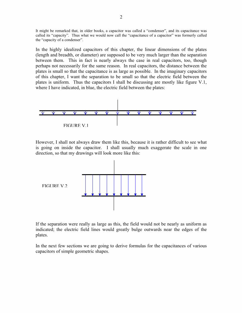
2

It might be remarked that, in older books, a capacitor was called a “condenser”, and its capacitance was called its “capacity”. Thus what we would now call the “capacitance of a capacitor” was formerly called the “capacity of a condenser”. In the highly idealized capacitors of this chapter, the linear dimensions of the plates (length and breadth, or diameter) are supposed to be very much larger than the separation between them. This in fact is nearly always the case in real capacitors, too, though perhaps not necessarily for the same reason. In real capacitors, the distance between the plates is small so that the capacitance is as large as possible. In the imaginary capacitors of this chapter, I want the separation to be small so that the electric field between the plates is uniform. Thus the capacitors I shall be discussing are mostly like figure V.1, where I have indicated, in blue, the electric field between the plates: However, I shall not always draw them like this, because it is rather difficult to see what is going on inside the capacitor. I shall usually much exaggerate the scale in one direction, so that my drawings will look more like this: If the separation were really as large as this, the field would not be nearly as uniform as indicated; the electric field lines would greatly bulge outwards near the edges of the plates. In the next few sections we are going to derive formulas for the capacitances of various capacitors of simple geometric shapes.

FIGURE V.1

FIGURE V.2

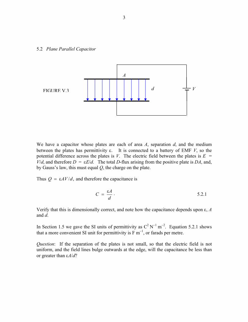
3

5.2 Plane Parallel Capacitor We have a capacitor whose plates are each of area A, separation d, and the medium between the plates has permittivity ε. It is connected to a battery of EMF V, so the potential difference across the plates is V. The electric field between the plates is E = V/d, and therefore D = εE/d. The total D-flux arising from the positive plate is DA, and, by Gauss’s law, this must equal Q, the charge on the plate. Thus ,/dAVQ ε= and therefore the capacitance is

.dAC ε

= 5.2.1

Verify that this is dimensionally correct, and note how the capacitance depends upon ε, A and d. In Section 1.5 we gave the SI units of permittivity as C2 N−1 m−2. Equation 5.2.1 shows that a more convenient SI unit for permittivity is F m−1, or farads per metre. Question: If the separation of the plates is not small, so that the electric field is not uniform, and the field lines bulge outwards at the edge, will the capacitance be less than or greater than εA/d?

FIGURE V.3 V

A

d

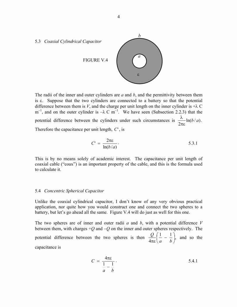
4

5.3 Coaxial Cylindrical Capacitor The radii of the inner and outer cylinders are a and b, and the permittivity between them is ε. Suppose that the two cylinders are connected to a battery so that the potential difference between them is V, and the charge per unit length on the inner cylinder is +λ C m−1, and on the outer cylinder is −λ C m−1. We have seen (Subsection 2.2.3) that the

potential difference between the cylinders under such circumstances is .)/ln(2

abπελ

Therefore the capacitance per unit length, 'C , is

.)/ln(

2'ab

C πε= 5.3.1

This is by no means solely of academic interest. The capacitance per unit length of coaxial cable (“coax”) is an important property of the cable, and this is the formula used to calculate it. 5.4 Concentric Spherical Capacitor Unlike the coaxial cylindrical capacitor, I don’t know of any very obvious practical application, nor quite how you would construct one and connect the two spheres to a battery, but let’s go ahead all the same. Figure V.4 will do just as well for this one. The two spheres are of inner and outer radii a and b, with a potential difference V between them, with charges +Q and −Q on the inner and outer spheres respectively. The

potential difference between the two spheres is then ,114

−

πε baQ and so the

capacitance is

.11

4

ba

C−

πε= 5.4.1

a

ε

b

FIGURE V.4

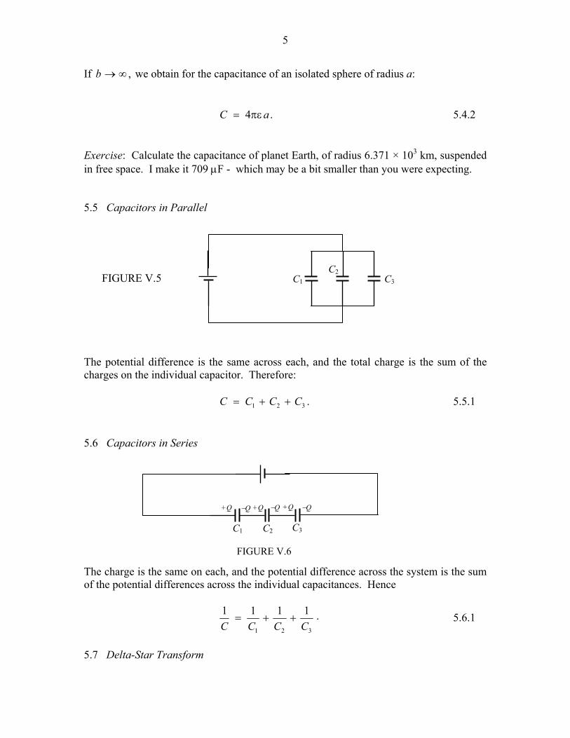
5

If ,∞→b we obtain for the capacitance of an isolated sphere of radius a: .4 aC πε= 5.4.2 Exercise: Calculate the capacitance of planet Earth, of radius 6.371 × 103 km, suspended in free space. I make it 709 µF - which may be a bit smaller than you were expecting. 5.5 Capacitors in Parallel The potential difference is the same across each, and the total charge is the sum of the charges on the individual capacitor. Therefore: .321 CCCC ++= 5.5.1 5.6 Capacitors in Series The charge is the same on each, and the potential difference across the system is the sum of the potential differences across the individual capacitances. Hence

.1111

321 CCCC++= 5.6.1


C1 C3

C2 FIGURE V.5

C1 C2 C3

+Q +Q +Q −Q −Q −Q

FIGURE V.6

6

As we did with resistors in Section 4.12, we can make a delta-star transform with capacitors. I leave it to the reader to show that the capacitance between any two terminals in the left hand box is the same as the capacitance between the corresponding two terminals in the right hand box provided that

,1

2113321 C

CCCCCCc ++= 5.7.1

2

2113322 C

CCCCCCc ++= 5.7.2

and .3

2113323 C

CCCCCCc ++= 5.7.3

The converse relations are

,321

321 ccc

ccC++

= 5.7.4

321

132 ccc

ccC++

= 5.7.5

and .321

213 ccc

ccC++

= 5.7.6

Z

X

Z

• •

•

Y

c1 c2

c3

FIGURE V.7

X

C1

C3

C2

• •

•

Y

7

For example, just for fun, what is the capacitance between points A and B in figure V.8, in which I have marked the individual capacitances in microfarads? The first three capacitors are connected in delta. Replace them by their equivalent star configuration. After that it should be straightforward. I make the answer 0.402 µF. 5.8 Kirchhoff’s Rules We can even adapt Kirchhoff’s rules to deal with capacitors. Thus, connect a 24 V battery across the circuit of figure V.8 – see figure V.9 Calculate the charge held in each capacitor. We can proceed in a manner very similar to how we did it in Chapter 4, applying the capacitance equivalent of Kirchhoff’s second rule to three closed circuits, and then making up the five necessary equations by applying “Kirchhoff’s first rule” to two points. Thus:

,023

24 32 =−−QQ 5.8.1

,08

24 42 =−−

QQ 5.8.2

•B A•

FIGURE V.8

3 2

4

1 8

FIGURE V.9

3 2

4

1 8

24 V

+Q1

+Q2 −Q2

+Q3 −Q3

+Q4 −Q4

+Q5

−Q5

−Q1

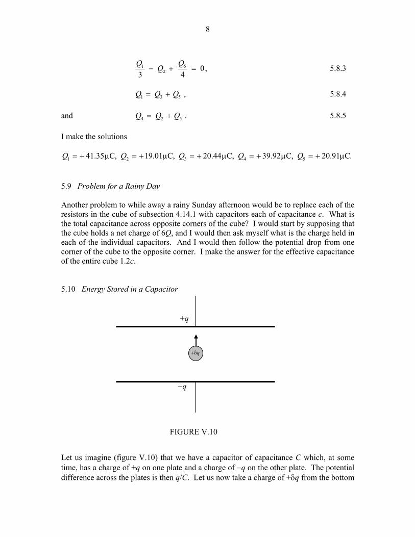
8

,043

52

1 =+−QQQ 5.8.3

,531 QQQ += 5.8.4 and .524 QQQ += 5.8.5 I make the solutions

.C91.20,C92.39,C44.20,C01.19,C35.41 54321 µ+=µ+=µ+=µ+=µ+= QQQQQ 5.9 Problem for a Rainy Day Another problem to while away a rainy Sunday afternoon would be to replace each of the resistors in the cube of subsection 4.14.1 with capacitors each of capacitance c. What is the total capacitance across opposite corners of the cube? I would start by supposing that the cube holds a net charge of 6Q, and I would then ask myself what is the charge held in each of the individual capacitors. And I would then follow the potential drop from one corner of the cube to the opposite corner. I make the answer for the effective capacitance of the entire cube 1.2c. 5.10 Energy Stored in a Capacitor Let us imagine (figure V.10) that we have a capacitor of capacitance C which, at some time, has a charge of +q on one plate and a charge of −q on the other plate. The potential difference across the plates is then q/C. Let us now take a charge of +δq from the bottom

+q

+δq

−q

FIGURE V.10

9

plate (the negative one) and move it up to the top plate. We evidently have to do work to

do this, in the amount of .qCq

δ The total work required, then, starting with the plates

completely uncharged until we have transferred a charge Q from one plate to the other is

).2/(1 2

0CQdqq

CQ

=∫ This is, then, the energy E stored in the capacitor, and, by

application of Q = CV it can also be written ,21 QV=E or, more usually,

.2

21 CV=E 5.10.1

Verify that this has the correct dimensions for energy. Also, think about how many expressions for energy you know that are of the form .2

21 ab There are more to come.

The symbol E is becoming rather over-worked. At present I am using the following: E = magnitude of the electric field E = electric field as a vector E = electromotive force E = energy Sorry about that! 5.11 Energy Stored in an Electric Field Recall that we are assuming that the separation between the plates is small compared with their linear dimensions and that therefore the electric field is uniform between the plates. The capacitance is dAC /ε= , and the potential differnece between the plates is Ed, where E is the electric field and d is the distance between the plates. Thus the energy stored in the capacitor is .2

21 AdEε The volume of the dielectric (insulating) material

between the plates is Ad, and therefore we find the following expression for the energy stored per unit volume in a dielectric material in which there is an electric field: .2

21 Eε

Verify that this has the correct dimensions for energy per unit volume. If the space between the plates is a vacuum, we have the following expression for the enrgy stored ber unit volume in the electric field 2

021 Eε

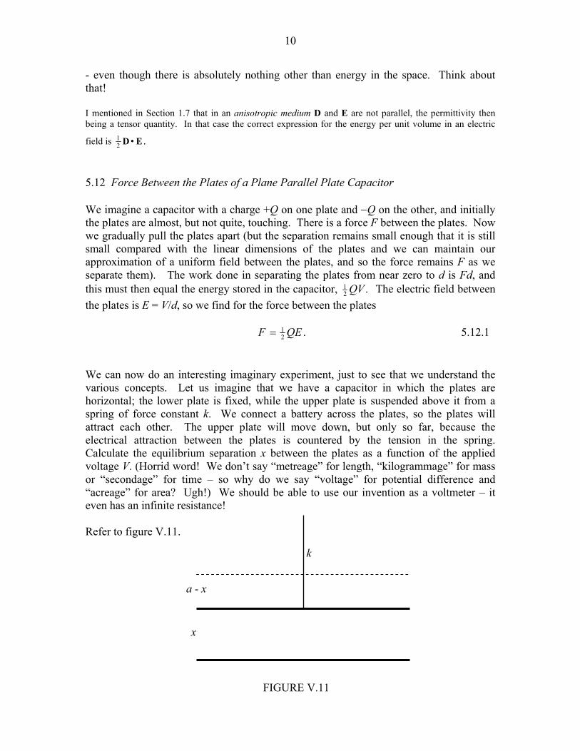
10

- even though there is absolutely nothing other than energy in the space. Think about that! I mentioned in Section 1.7 that in an anisotropic medium D and E are not parallel, the permittivity then being a tensor quantity. In that case the correct expression for the energy per unit volume in an electric

field is .21 ED •

5.12 Force Between the Plates of a Plane Parallel Plate Capacitor We imagine a capacitor with a charge +Q on one plate and −Q on the other, and initially the plates are almost, but not quite, touching. There is a force F between the plates. Now we gradually pull the plates apart (but the separation remains small enough that it is still small compared with the linear dimensions of the plates and we can maintain our approximation of a uniform field between the plates, and so the force remains F as we separate them). The work done in separating the plates from near zero to d is Fd, and this must then equal the energy stored in the capacitor, .2

1 QV The electric field between the plates is E = V/d, so we find for the force between the plates .2

1 QEF = 5.12.1 We can now do an interesting imaginary experiment, just to see that we understand the various concepts. Let us imagine that we have a capacitor in which the plates are horizontal; the lower plate is fixed, while the upper plate is suspended above it from a spring of force constant k. We connect a battery across the plates, so the plates will attract each other. The upper plate will move down, but only so far, because the electrical attraction between the plates is countered by the tension in the spring. Calculate the equilibrium separation x between the plates as a function of the applied voltage V. (Horrid word! We don’t say “metreage” for length, “kilogrammage” for mass or “secondage” for time – so why do we say “voltage” for potential difference and “acreage” for area? Ugh!) We should be able to use our invention as a voltmeter – it even has an infinite resistance! Refer to figure V.11.

k

x

a - x

FIGURE V.11

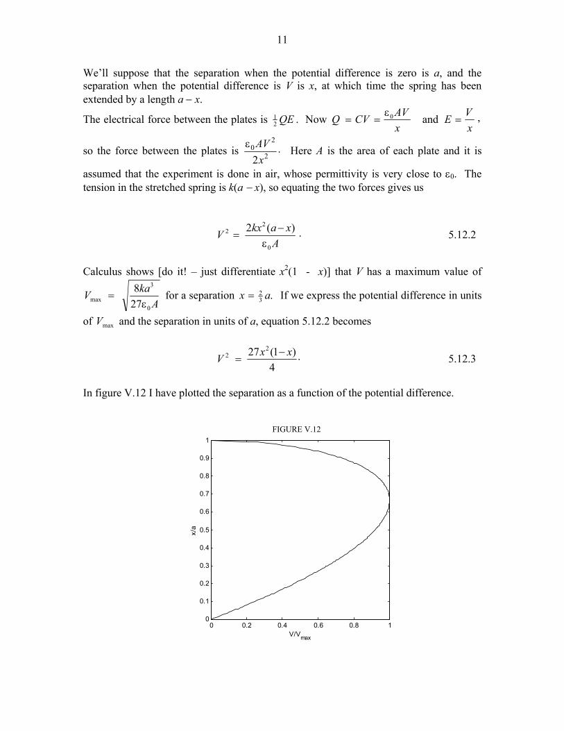
11

We’ll suppose that the separation when the potential difference is zero is a, and the separation when the potential difference is V is x, at which time the spring has been extended by a length a − x.

The electrical force between the plates is QE21 . Now ,and0

xVE

xAVCVQ =

ε==

so the force between the plates is .2 2

20

xAVε Here A is the area of each plate and it is

assumed that the experiment is done in air, whose permittivity is very close to ε0. The tension in the stretched spring is k(a − x), so equating the two forces gives us

.)(2

0

22

AxakxV

ε−

= 5.12.2

Calculus shows [do it! – just differentiate x2(1 - x)] that V has a maximum value of

AkaV

0

3

max 278

ε= for a separation .3

2 ax = If we express the potential difference in units

of maxV and the separation in units of a, equation 5.12.2 becomes

.4

)1(27 22 xxV −

= 5.12.3

In figure V.12 I have plotted the separation as a function of the potential difference.

0 0.2 0.4 0.6 0.8 1

0

0.1

0.2

0.3

0.4

0.5

0.6

0.7

0.8

0.9

1

V/Vmax

x/a

FIGURE V.10

FIGURE V.12

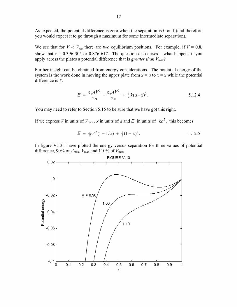
12

As expected, the potential difference is zero when the separation is 0 or 1 (and therefore you would expect it to go through a maximum for some intermediate separation). We see that for maxVV < there are two equilibrium positions. For example, if V = 0.8, show that x = 0.396 305 or 0.876 617. The question also arises – what happens if you apply across the plates a potential difference that is greater than Vmax? Further insight can be obtained from energy considerations. The potential energy of the system is the work done in moving the upper plate from x = a to x = x while the potential difference is V:

.)(22

221

20

20 xak

xAV

aAV

−+ε

−ε

=E 5.12.4

You may need to refer to Section 5.15 to be sure that we have got this right. If we express V in units of Vmax , x in units of a and E in units of ,2ka this becomes .)1()/11( 2

212

274 xxV −+−=E 5.12.5

In figure V.13 I have plotted the energy versus separation for three values of potential difference, 90% of Vmax, Vmax and 110% of Vmax.

0 0.1 0.2 0.3 0.4 0.5 0.6 0.7 0.8 0.9 1-0.1

-0.08

-0.06

-0.04

-0.02

0

0.02

x

Pot

entia

l ene

rgy

FIGURE V.13

V = 0.90

1.00

1.10

13

We see that for V < Vmax, there are two equilibrium positions, of which the lower one (smaller x) is unstable, and we see exactly what will happen if the upper plate is displaced slightly upwards (larger x) from the unstable equilibrium position or if it is displaced slightly downwards (smaller x). The upper equilibrium position is stable. If V > Vmax, there is no equilibrium position, and x goes down to zero – i.e. the plates clamp together. 5.13 Sharing a Charge Between Two Capacitors We have two capacitors. C2 is initially uncharged. Initially,C1 bears a charge Q0 and the potential difference across its plates is V0, such that ,010 VCQ = 5.13.1 and the energy of the system is .2

0121

0 VC=E 5.13.2 We now close the switches, so that the charge is shared between the two capacitors: The capacitors C1 and C2 now bear charges Q1 and Q2 such that Q0 = Q1 + Q2 and

021

11 Q

CCCQ+

= and .021

22 Q

CCCQ+

= 5.13.3a,b

Q0 C1 V0

FIGURE V.14

C2

Q1 C1 V

FIGURE V.15

Q2 C2 V

14

The potential difference across the plates of either capacitor is, of course, the same, so we can call it V without a subscript, and it is easily seen, by applying Q = CV to either capacitor, that

.021

1 VCC

CV+

= 5.13.4

We can now apply 2

21 CV=E to each capacitor in turn to find the energy stored in each.

We find for the energies stored in the two capacitors:

221

20

31

1 )(2 CCVC+

=E and .)(2 2

21

20

212

2 CCVCC

+=E 5.13.5a,b

The total energy stored in the two capacitors is the sum of these, which is

,)(2 21

20

21

CCVC+

=E 5.13.6

which can also be written

.021

1 EECC

C+

= 5.13.7

Surprise, surprise! The energy stored in the two capacitors is less than the energy that was originally stored in C1. What has happened to the lost energy? A perfectly reasonable and not incorrect answer is that it has been dissipated as heat in the connecting wires as current flowed from one capacitor to the other. However, it has been found in low temperature physics that if you immerse certain metals in liquid helium they lose all electrical resistance and they become superconductive. So, let us connect the capacitors with superconducting wires. Then there is no dissipation of energy as heat in the wires – so the question remains: where has the missing energy gone? Well, perhaps the dielectric medium in the capacitors is heated? Again this seems like a perfectly reasonable and probably not entirely incorrect answer. However, my capacitors have a vacuum between the plates, and are connected by superconducting wires, so that no heat is generated either in the dielectric or in the wires. Where has that energy gone? This will have to remain a mystery for the time being, and a topic for lunchtime conversation. In a later chapter I shall suggest another explanation.

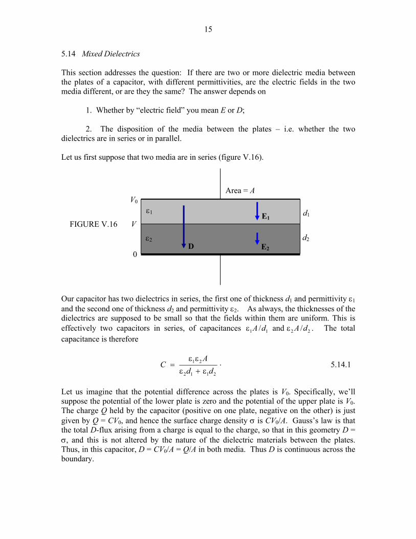
15

5.14 Mixed Dielectrics This section addresses the question: If there are two or more dielectric media between the plates of a capacitor, with different permittivities, are the electric fields in the two media different, or are they the same? The answer depends on 1. Whether by “electric field” you mean E or D; 2. The disposition of the media between the plates – i.e. whether the two dielectrics are in series or in parallel. Let us first suppose that two media are in series (figure V.16). Our capacitor has two dielectrics in series, the first one of thickness d1 and permittivity ε1

and the second one of thickness d2 and permittivity ε2. As always, the thicknesses of the dielectrics are supposed to be small so that the fields within them are uniform. This is effectively two capacitors in series, of capacitances ./and/ 2211 dAdA εε The total capacitance is therefore

.2112

21

ddA

Cε+ε

εε= 5.14.1

Let us imagine that the potential difference across the plates is V0. Specifically, we’ll suppose the potential of the lower plate is zero and the potential of the upper plate is V0. The charge Q held by the capacitor (positive on one plate, negative on the other) is just given by Q = CV0, and hence the surface charge density σ is CV0/A. Gauss’s law is that the total D-flux arising from a charge is equal to the charge, so that in this geometry D = σ, and this is not altered by the nature of the dielectric materials between the plates. Thus, in this capacitor, D = CV0/A = Q/A in both media. Thus D is continuous across the boundary.

FIGURE V.16

0

V0

V

d1 ε1

D

E1

d2 ε2 E2

Area = A

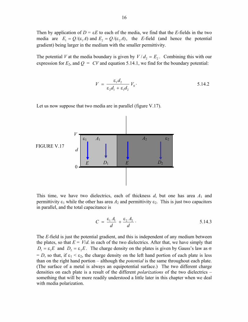
16

Then by application of D = εE to each of the media, we find that the E-fields in the two media are ,)/(and)/( 2211 AQEAQE ε=ε= the E-field (and hence the potential gradient) being larger in the medium with the smaller permittivity. The potential V at the media boundary is given by ./ 22 EdV = Combining this with our expression for E2, and Q = CV and equation 5.14.1, we find for the boundary potential:

.0

2112

21 Vdd

dV

ε+ε

ε= 5.14.2

Let us now suppose that two media are in parallel (figure V.17). This time, we have two dielectrics, each of thickness d, but one has area A1 and permittivity ε1 while the other has area A2 and permittivity ε2. This is just two capacitors in parallel, and the total capacitance is

.2211

dA

dAC ε

+ε

= 5.14.3

The E-field is just the potential gradient, and this is independent of any medium between the plates, so that E = V/d. in each of the two dielectrics. After that, we have simply that

.and 2211 EDED ε=ε= The charge density on the plates is given by Gauss’s law as σ = D, so that, if ε1 < ε2, the charge density on the left hand portion of each plate is less than on the right hand portion – although the potential is the same throughout each plate. (The surface of a metal is always an equipotential surface.) The two different charge densities on each plate is a result of the different polarizations of the two dielectrics – something that will be more readily understood a little later in this chapter when we deal with media polarization.

0

d

E D1

ε2 ε1

FIGURE V.17

V A1 A2

D2 E

17

We have established that: 1. The component of D perpendicular to a boundary is continuous; 2. The component of E parallel to a boundary is continuous. In figure V.18 we are looking at the D-field and at the E-field as it crosses a boundary in which ε1 < ε2. Note that Dy and Ex are the same on either side of the boundary. This results in:

.tantan

2

1

2

1

εε

=θθ 5.14.4

5.15 Changing the Distance Between the Plates of a Capacitor If you gradually increase the distance between the plates of a capacitor (although always keeping it sufficiently small so that the field is uniform) does the intensity of the field change or does it stay the same? If the former, does it increase or decrease? The answer to these questions depends 1. on whether, by the field, you are referring to the E-field or the D-field; 2. on whether the plates are isolated or if they are connected to the poles of a battery. We shall start by supposing that the plates are isolated.

ε1

ε2

ε1Ey/ε2

Dx

Dy

θ1

θ2

Dy

ε2Dx/ε1

Ex

Ey

θ1

θ2

Ex

FIGURE V.18

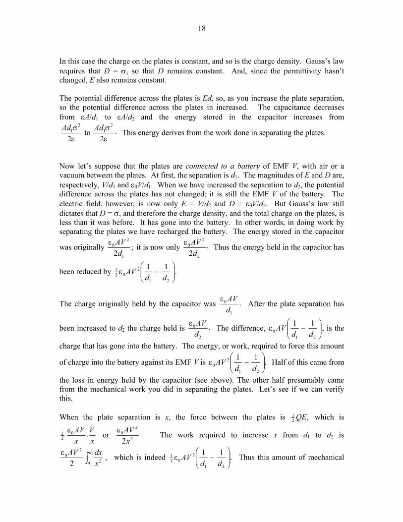
18

In this case the charge on the plates is constant, and so is the charge density. Gauss’s law requires that D = σ, so that D remains constant. And, since the permittivity hasn’t changed, E also remains constant. The potential difference across the plates is Ed, so, as you increase the plate separation, so the potential difference across the plates in increased. The capacitance decreases from εA/d1 to εA/d2 and the energy stored in the capacitor increases from

.2

to2

21

21

εσ

εσ AdAd This energy derives from the work done in separating the plates.

Now let’s suppose that the plates are connected to a battery of EMF V, with air or a vacuum between the plates. At first, the separation is d1. The magnitudes of E and D are, respectively, V/d1 and ε0V/d1. When we have increased the separation to d2, the potential difference across the plates has not changed; it is still the EMF V of the battery. The electric field, however, is now only E = V/d2 and D = ε0V/d2. But Gauss’s law still dictates that D = σ, and therefore the charge density, and the total charge on the plates, is less than it was before. It has gone into the battery. In other words, in doing work by separating the plates we have recharged the battery. The energy stored in the capacitor

was originally ;2 1

20

dAVε it is now only .

2 2

20

dAVε Thus the energy held in the capacitor has

been reduced by .11

21

202

1

−ε

ddAV

The charge originally held by the capacitor was .1

0

dAVε After the plate separation has

been increased to d2 the charge held is .2

0

dAVε The difference,

−ε

210

11dd

AV , is the

charge that has gone into the battery. The energy, or work, required to force this amount

of charge into the battery against its EMF V is .11

21

20

−ε

ddAV Half of this came from

the loss in energy held by the capacitor (see above). The other half presumably came from the mechanical work you did in separating the plates. Let’s see if we can verify this. When the plate separation is x, the force between the plates is ,2

1 QE which is

.2

or.2

200

21

xAV

xV

xAV εε The work required to increase x from d1 to d2 is

,2

2

12

20 ∫

ε d

d xdxAV which is indeed .11

21

202

1

−ε

ddAV Thus this amount of mechanical

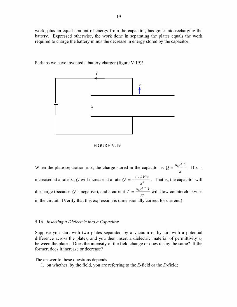
19

work, plus an equal amount of energy from the capacitor, has gone into recharging the battery. Expressed otherwise, the work done in separating the plates equals the work required to charge the battery minus the decrease in energy stored by the capacitor. Perhaps we have invented a battery charger (figure V.19)!

When the plate separation is x, the charge stored in the capacitor is .0

xAVQ ε

= If x is

increased at a rate x& , Q will increase at a rate .20

xxAVQ&& ε

−= That is, the capacitor will

discharge (because Q& is negative), and a current 20

xxAVI&ε

= will flow counterclockwise

in the circuit. (Verify that this expression is dimensionally correct for current.) 5.16 Inserting a Dielectric into a Capacitor Suppose you start with two plates separated by a vacuum or by air, with a potential difference across the plates, and you then insert a dielectric material of permittivity ε0 between the plates. Does the intensity of the field change or does it stay the same? If the former, does it increase or decrease? The answer to these questions depends 1. on whether, by the field, you are referring to the E-field or the D-field;

x

I

FIGURE V.19

x&

20

2. on whether the plates are isolated or if they are connected to the poles of a battery. We shall start by supposing that the plates are isolated. See figure V.20. Let Q be the charge on the plates, and σ the surface charge density. These are unaltered by the introduction of the dielectric. Gauss’s law provides that D = σ, so this, too, is unaltered by the introduction of the dielectric. The electric field was, initially,

./ 01 ε= DE After introduction of the dielectric, it is a little less, namely ./1 ε= DE Let us take the potential of the lower plate to be zero. Before introduction of the dielectric, the potential of the upper plate was ./ 01 εσ= dV After introduction of the dielectric, it is a little less, namely ./1 εσ= dV Why is the electric field E less after introduction of the dielectric material? It is because the dielectric material becomes polarized. We saw in Section 3.6 how matter may become polarized. Either molecules with pre-existing dipole moments align themselves with the imposed electric field, or, if they have no permanent dipole moment or if they cannot rotate, a dipole moment can be induced in the individual molecules. In any case, the effect of the alignment of all these molecular dipoles is that there is a slight surplus of positive charge on the surface of the dielectric material next to the negative plate, and a slight surplus of negative charge on the surface of the dielectric material next to the positive plate. This produces an electric field opposite to the direction of the imposed field, and thus the total electric field is somewhat reduced. Before introduction of the dielectric material, the energy stored in the capacitor was

121 QV . After introduction of the material, it is ,22

1 QV which is a little bit less. Thus it will require work to remove the material from between the plates. The empty capacitor

V1 = σd/ε0

FIGURE V.20

− − − − − − − − − − − − − − − − − − − − − −

+ + + + + + + + + + + + + + + + + + + + + +

0

ε ε0

σ Q = σA Q = σA σ

V2 = σd/ε

0 D = σ E2 = D/ε D = σ E1 = D/ε0

− − − − − − −

+ + + + +

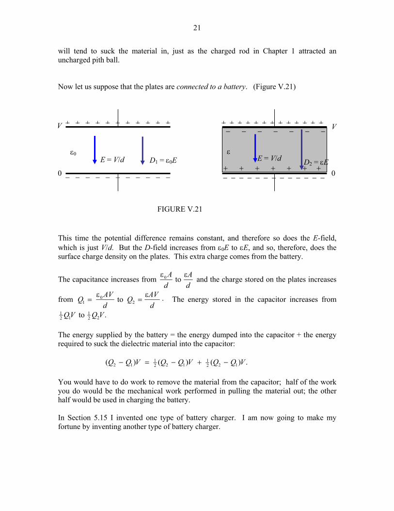
21

will tend to suck the material in, just as the charged rod in Chapter 1 attracted an uncharged pith ball. Now let us suppose that the plates are connected to a battery. (Figure V.21) This time the potential difference remains constant, and therefore so does the E-field, which is just V/d. But the D-field increases from ε0E to εE, and so, therefore, does the surface charge density on the plates. This extra charge comes from the battery.

The capacitance increases from dA

dA εε to0 and the charge stored on the plates increases

from .to 20

1 dAVQ

dAVQ ε

=ε

= The energy stored in the capacitor increases from

.to 221

121 VQVQ The energy supplied by the battery = the energy dumped into the capacitor + the energy required to suck the dielectric material into the capacitor: .)()()( 122

1122

112 VQQVQQVQQ −+−=−

You would have to do work to remove the material from the capacitor; half of the work you do would be the mechanical work performed in pulling the material out; the other half would be used in charging the battery. In Section 5.15 I invented one type of battery charger. I am now going to make my fortune by inventing another type of battery charger.

V

FIGURE V.21

− − − − − − − − − − − − − − − − − − − − − − − −

+ + + + + + + + + + + + + + + + + + + + + + + +

0

ε ε0

V

0

D2 = εE E = V/d D1 = ε0E

− − − − − − −

+ + + + + + +

E = V/d

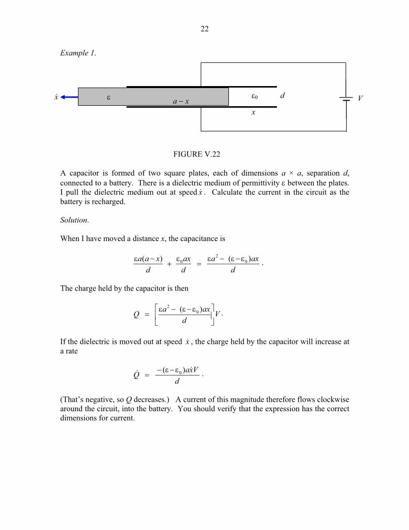
22

Example 1. A capacitor is formed of two square plates, each of dimensions a × a, separation d, connected to a battery. There is a dielectric medium of permittivity ε between the plates. I pull the dielectric medium out at speed x& . Calculate the current in the circuit as the battery is recharged. Solution. When I have moved a distance x, the capacitance is

.)()( 02

0

daxa

dax

dxaa ε−ε−ε

=ε

+−ε

The charge held by the capacitor is then

.)( 02

Vd

axaQ

ε−ε−ε=

If the dielectric is moved out at speed x& , the charge held by the capacitor will increase at a rate

.)( 0

dVxaQ&& ε−ε−

=

(That’s negative, so Q decreases.) A current of this magnitude therefore flows clockwise around the circuit, into the battery. You should verify that the expression has the correct dimensions for current.

ε ε0 x&

x a − x

d

FIGURE V.22

V

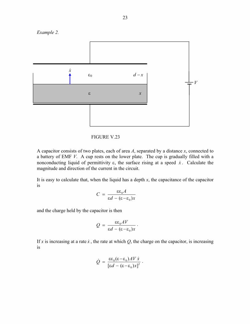
23

Example 2. A capacitor consists of two plates, each of area A, separated by a distance x, connected to a battery of EMF V. A cup rests on the lower plate. The cup is gradually filled with a nonconducting liquid of permittivity ε, the surface rising at a speed x& . Calculate the magnitude and direction of the current in the circuit. It is easy to calculate that, when the liquid has a depth x, the capacitance of the capacitor is

xd

AC)( 0

0

ε−ε−εεε

=

and the charge held by the capacitor is then

.)( 0

0

xdAVQ

ε−ε−εεε

=

If x is increasing at a rate x& , the rate at which Q, the charge on the capacitor, is increasing is

.])([

)(2

0

00

xdxAVQ

ε−ε−εε−εεε

=&&

FIGURE V.23

d − x

x

V ε0

x&

ε

24

A current of this magnitude therefore flows in the circuit counterclockwise, draining the

battery. This current increases monotonically from zero to .)(2

0

0

dxAV

εε−εε &

5.17 Polarization and Susceptibility When an insulating material is placed in an electric field, it becomes polarized, either by rotation of molecules with pre-existing dipole moments or by induction of dipole moments in the individual molecules. Inside the material, D is then greater than ε0E. Indeed, .0 PED +ε= 5.17.1 The excess, P, of D over ε0E is called the polarization of the medium. It is dimensionally similar to, and expressed in the same units as, D; that is to say C m−2. Another way of looking at the polarization of a medium is that it is the dipole moment per unit volume. In vector form, the relation is .0 PED +ε= 5.17.2 If the medium is isotropic, all three vectors are parallel. Some media are more susceptible to becoming polarized in a polarizing field than others, and the ratio of P to ε0E is called the electric susceptibility χe of the medium: .0e EP εχ= 5.17.3 This implies that P is linearly proportional to E but only if χe is independent of E, which is by no means always the case, but is good for small polarizations. When we combine equations 5.17.1 and 5.17.3 with D = εE and with ,/ 0r εε=ε the relative permittivity or dielectric constant, we obtain .1re −ε=χ 5.17.4

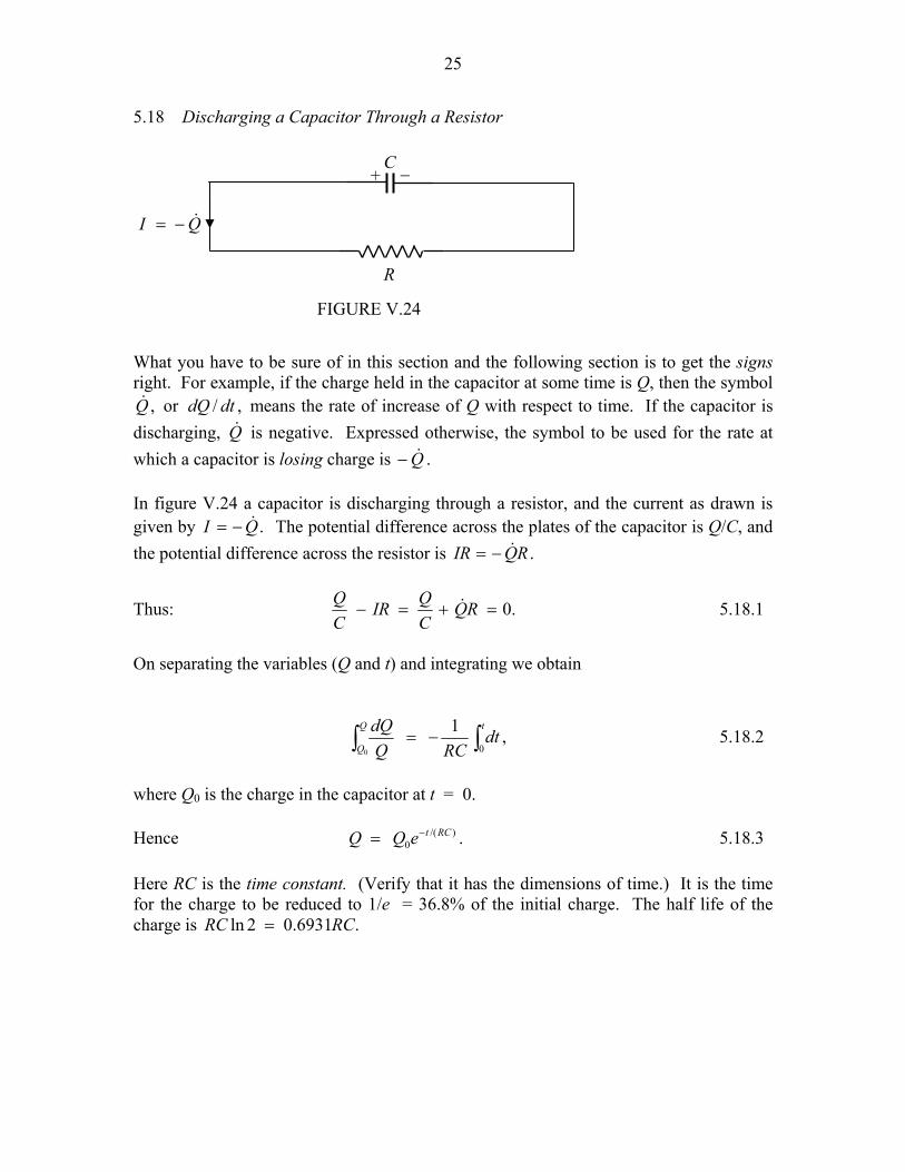
25

5.18 Discharging a Capacitor Through a Resistor What you have to be sure of in this section and the following section is to get the signs right. For example, if the charge held in the capacitor at some time is Q, then the symbol

,/or, dtdQQ& means the rate of increase of Q with respect to time. If the capacitor is discharging, Q& is negative. Expressed otherwise, the symbol to be used for the rate at which a capacitor is losing charge is Q&− . In figure V.24 a capacitor is discharging through a resistor, and the current as drawn is given by .QI &−= The potential difference across the plates of the capacitor is Q/C, and the potential difference across the resistor is .RQIR &−=

Thus: .0=+=− RQCQIR

CQ & 5.18.1

On separating the variables (Q and t) and integrating we obtain

,100

∫∫ −=tQ

Qdt

RCQdQ 5.18.2

where Q0 is the charge in the capacitor at t = 0. Hence .)/(

0RCteQQ −= 5.18.3

Here RC is the time constant. (Verify that it has the dimensions of time.) It is the time for the charge to be reduced to 1/e = 36.8% of the initial charge. The half life of the charge is .6931.02ln RCRC =

FIGURE V.24

R

+ −

QI &−=

C

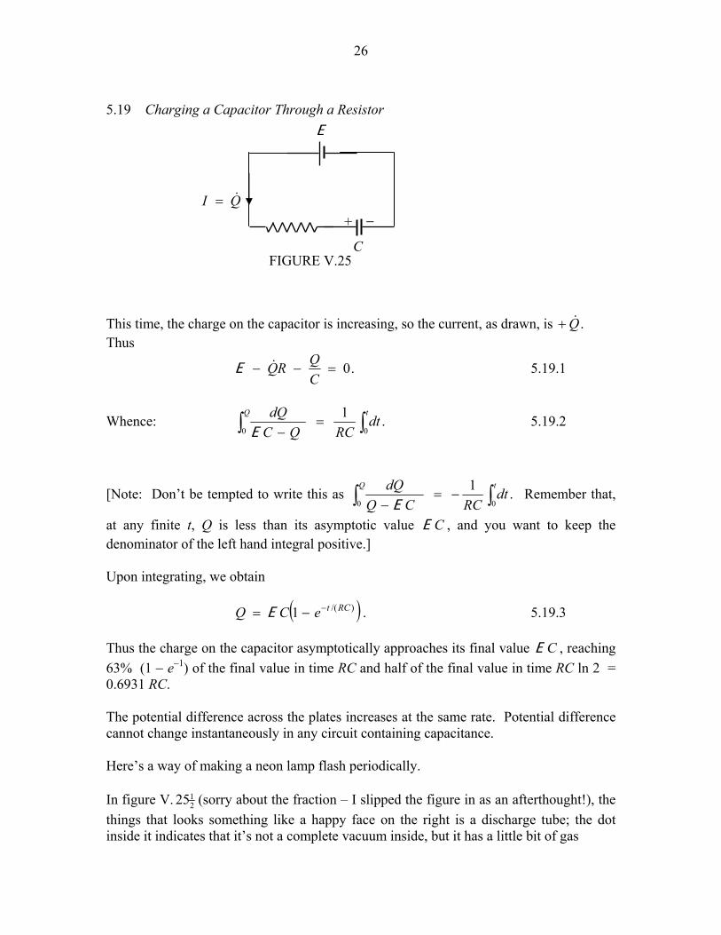
26

5.19 Charging a Capacitor Through a Resistor This time, the charge on the capacitor is increasing, so the current, as drawn, is .Q&+ Thus

.0=−−CQRQ&E 5.19.1

Whence: ∫∫ =−

tQdt

RCQCdQ

00.1

E 5.19.2

[Note: Don’t be tempted to write this as ∫∫ −=−

tQdt

RCCQdQ

00.1

E Remember that,

at any finite t, Q is less than its asymptotic value CE , and you want to keep the denominator of the left hand integral positive.] Upon integrating, we obtain ( ) .1 )/(RCteCQ −−= E 5.19.3 Thus the charge on the capacitor asymptotically approaches its final value CE , reaching 63% (1 − e−1) of the final value in time RC and half of the final value in time RC ln 2 = 0.6931 RC. The potential difference across the plates increases at the same rate. Potential difference cannot change instantaneously in any circuit containing capacitance. Here’s a way of making a neon lamp flash periodically. In figure V. 2

125 (sorry about the fraction – I slipped the figure in as an afterthought!), the things that looks something like a happy face on the right is a discharge tube; the dot inside it indicates that it’s not a complete vacuum inside, but it has a little bit of gas

QI &=

FIGURE V.25 C

E

+ −

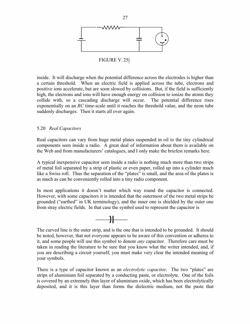
27

inside. It will discharge when the potential difference across the electrodes is higher than a certain threshold. When an electric field is applied across the tube, electrons and positive ions accelerate, but are soon slowed by collisions. But, if the field is sufficiently high, the electrons and ions will have enough energy on collision to ionize the atoms they collide with, so a cascading discharge will occur. The potential difference rises exponentially on an RC time-scale until it reaches the threshold value, and the neon tube suddenly discharges. Then it starts all over again. 5.20 Real Capacitors Real capacitors can vary from huge metal plates suspended in oil to the tiny cylindrical components seen inside a radio. A great deal of information about them is available on the Web and from manufacturers’ catalogues, and I only make the briefest remarks here. A typical inexpensive capacitor seen inside a radio is nothing much more than two strips of metal foil separated by a strip of plastic or even paper, rolled up into a cylinder much like a Swiss roll. Thus the separation of the “plates” is small, and the area of the plates is as much as can be conveniently rolled into a tiny radio component. In most applications it doesn’t matter which way round the capacitor is connected. However, with some capacitors it is intended that the outermost of the two metal strips be grounded (“earthed” in UK terminology), and the inner one is shielded by the outer one from stray electric fields. In that case the symbol used to represent the capacitor is The curved line is the outer strip, and is the one that is intended to be grounded. It should be noted, however, that not everyone appears to be aware of this convention or adheres to it, and some people will use this symbol to denote any capacitor. Therefore care must be taken in reading the literature to be sure that you know what the writer intended, and, if you are describing a circuit yourself, you must make very clear the intended meaning of your symbols. There is a type of capacitor known as an electrolytic capacitor. The two “plates” are strips of aluminium foil separated by a conducting paste, or electrolyte. One of the foils is covered by an extremely thin layer of aluminium oxide, which has been electrolytically deposited, and it is this layer than forms the dielectric medium, not the paste that

FIGURE V. 2125

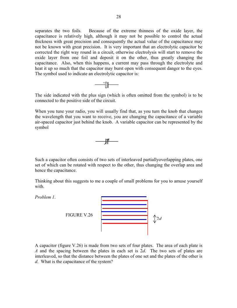
28

separates the two foils. Because of the extreme thinness of the oxide layer, the capacitance is relatively high, although it may not be possible to control the actual thickness with great precision and consequently the actual value of the capacitance may not be known with great precision. It is very important that an electrolytic capacitor be corrected the right way round in a circuit, otherwise electrolysis will start to remove the oxide layer from one foil and deposit it on the other, thus greatly changing the capacitance. Also, when this happens, a current may pass through the electrolyte and heat it up so much that the capacitor may burst open with consequent danger to the eyes. The symbol used to indicate an electrolytic capacitor is: The side indicated with the plus sign (which is often omitted from the symbol) is to be connected to the positive side of the circuit. When you tune your radio, you will usually find that, as you turn the knob that changes the wavelength that you want to receive, you are changing the capacitance of a variable air-spaced capacitor just behind the knob. A variable capacitor can be represented by the symbol Such a capacitor often consists of two sets of interleaved partiallyoverlapping plates, one set of which can be rotated with respect to the other, thus changing the overlap area and hence the capacitance. Thinking about this suggests to me a couple of small problems for you to amuse yourself with. Problem 1. A capacitor (figure V.26) is made from two sets of four plates. The area of each plate is A and the spacing between the plates in each set is 2d. The two sets of plates are interleaved, so that the distance between the plates of one set and the plates of the other is d. What is the capacitance of the system?

+

FIGURE V.26 2d

29

Problem 2 This is just like Problem 1, except that one set has four plates and the other has three. What is the capacitance now? Answers on the next page.

FIGURE V.27 2d

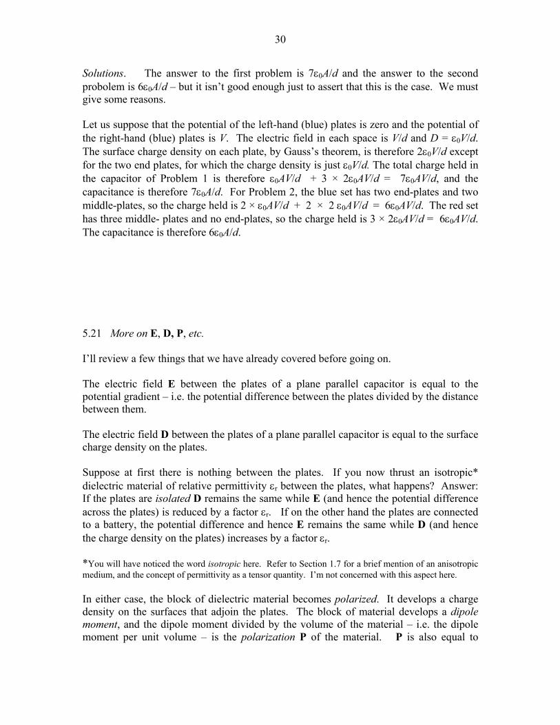
30

Solutions. The answer to the first problem is 7ε0A/d and the answer to the second probolem is 6ε0A/d – but it isn’t good enough just to assert that this is the case. We must give some reasons. Let us suppose that the potential of the left-hand (blue) plates is zero and the potential of the right-hand (blue) plates is V. The electric field in each space is V/d and D = ε0V/d. The surface charge density on each plate, by Gauss’s theorem, is therefore 2ε0V/d except for the two end plates, for which the charge density is just ε0V/d. The total charge held in the capacitor of Problem 1 is therefore ε0AV/d + 3 × 2ε0AV/d = 7ε0AV/d, and the capacitance is therefore 7ε0A/d. For Problem 2, the blue set has two end-plates and two middle-plates, so the charge held is 2 × ε0AV/d + 2 × 2 ε0AV/d = 6ε0AV/d. The red set has three middle- plates and no end-plates, so the charge held is 3 × 2ε0AV/d = 6ε0AV/d. The capacitance is therefore 6ε0A/d. 5.21 More on E, D, P, etc. I’ll review a few things that we have already covered before going on. The electric field E between the plates of a plane parallel capacitor is equal to the potential gradient – i.e. the potential difference between the plates divided by the distance between them. The electric field D between the plates of a plane parallel capacitor is equal to the surface charge density on the plates. Suppose at first there is nothing between the plates. If you now thrust an isotropic* dielectric material of relative permittivity εr between the plates, what happens? Answer: If the plates are isolated D remains the same while E (and hence the potential difference across the plates) is reduced by a factor εr. If on the other hand the plates are connected to a battery, the potential difference and hence E remains the same while D (and hence the charge density on the plates) increases by a factor εr. *You will have noticed the word isotropic here. Refer to Section 1.7 for a brief mention of an anisotropic medium, and the concept of permittivity as a tensor quantity. I’m not concerned with this aspect here. In either case, the block of dielectric material becomes polarized. It develops a charge density on the surfaces that adjoin the plates. The block of material develops a dipole moment, and the dipole moment divided by the volume of the material – i.e. the dipole moment per unit volume – is the polarization P of the material. P is also equal to

31

ED 0ε− and, of course, to EE 0ε−ε . The ratio of the resulting polarization P to the polarizing field ε0E is called the electric susceptibility χ of the medium. It will be worth spending a few moments convincing yourself from these definitions and concepts that

)1(0 χ+ε=ε and 1r −ε=χ , where rε is the dimensionless relative permittivity (or dielectric constant) 0/ εε . What is happening physically inside the medium when it becomes polarized? One possibility is that the individual molecules, if they are asymmetric molecules, may already possess a permanent dipole moment. The molecule carbon dioxide, which, in its ground state, is linear and symmetric, O=C=O, does not have a permanent dipole moment. Symmetric molecules such as CH4, and single atoms such as He, do not have a permanent dipole moment. The water molecule has some elements of symmetry, but it is not linear, and it does have a permanent dipole moment, of about 6 %10−30 C m, directed along the bisector of the HOH angle and away from the O atom. If the molecules have a permanent dipole moment and are free to rotate (as, for example, in a gas) they will tend to rotate in the direction of the applied field. (I’ll discuss that phrase “tend to” in a moment.) Thus the material becomes polarized. A molecule such as CH4 is symmetric and has no permanent dipole moment, but, if it is placed in an external electric field, the molecule may become distorted from its perfect tetrahedral shape with neat 109º angles, because each pair of CH atoms has a dipole moment. Thus the molecule acquires an induced dipole moment, and the material as a whole becomes polarized. The ratio of the induced dipole moment p to the polarizing field E polarizability α of the molecule. Review Section 3.6 for more on this. How about a single atom, such as Kr? Even that can acquire a dipole moment. Although there are no bonds to bend, under the influence of an electric field a preponderance of electrons will migrate to one side of the atom, and so the atom acquires a dipole moment. The same phenomenon applies, of course, to a molecule such as CH4 in addition to the bond bending already mentioned. Let us consider the situation of a dielectric material in which the molecules have a permanent dipole moment and are free (as in a gas, for example) to rotate. We’ll suppose that, at least in a weak polarizing field, the permanent dipole moment is significantly larger than any induced dipole moment, so we’ll neglect the latter. We have said that, under the influence of a polarizing field, the permanent dipole will tend to align themselves with the field. But they also have to contend with the constant jostling and collisions between molecules, which knock their dipole moments haywire, so they can’t immediately all align exactly with the field. We might imagine that the material may become fairly strongly polarized if the temperature is fairly low, but only relatively weakly polarized at higher temperatures. Dare we even hope that we might be able to predict the variation of polarization P with temperature T? Let’s have a go! We recall (Section 3.4) that the potential energy U of a dipole, when it makes an angle θ with the electric field, is .cos Ep •−=θ−= pEU The energy of a dipole whose

32

direction makes an angle of between θ and θ+θ d with the field will be between U and dUU + , where θθ= dpEdU sin . What happens next requires familiarity with

Boltzmann’s equation for distribution of energies in a statistical mechanics. See for example my Stellar Atmospheres notes, Chapter 8, Section 8.4. The fraction of molecules having energies between U and dUU + will be, following Boltzmann’s equation,

∫+−

−

−

pEpE

kTU

kTU

dUedUe

)/(

)/(’ 5.21.1

(Caution: Remember that here I’m using U for potential energy, and E for electric field.) That is, the fraction of molecules making angles of between θ and θ+θ d with the field is

∫∫π θ

θ

π θ

θ

θθ

θθ=

θθ

θθ

0)/(cos

)/(cos

0)/(cos

)/(cos

sinsin

sinsin

dede

dpEedpEe

kTpE

kTpE

kTpE

kTpE. 5.21.2

The component in the direction of E of the dipole moment of this fraction of the molecules is

∫π θ

θ

θθ

θθθ

0)/(cos

)/(cos

sincossin

dedpe

kTpE

kTpE, 5.21.3

so the component in the direction of E of the dipole moment all of the molecules is

∫

∫π θ−

π θ−

θθ

θθθ

0)/(cos

0)/(cos

sin

cossin

de

depkTpE

kTpE

, 5.21.4

and this expression represents the induced dipole moment in the direction of the field of the entire sample, which I’ll call ps. The polarization of the sample would be this divided by its volume.

Let θ=θ= coscos akTpEx . 5.21.5

Then the expression for the dipole moment of the entire sample becomes (some care is needed):

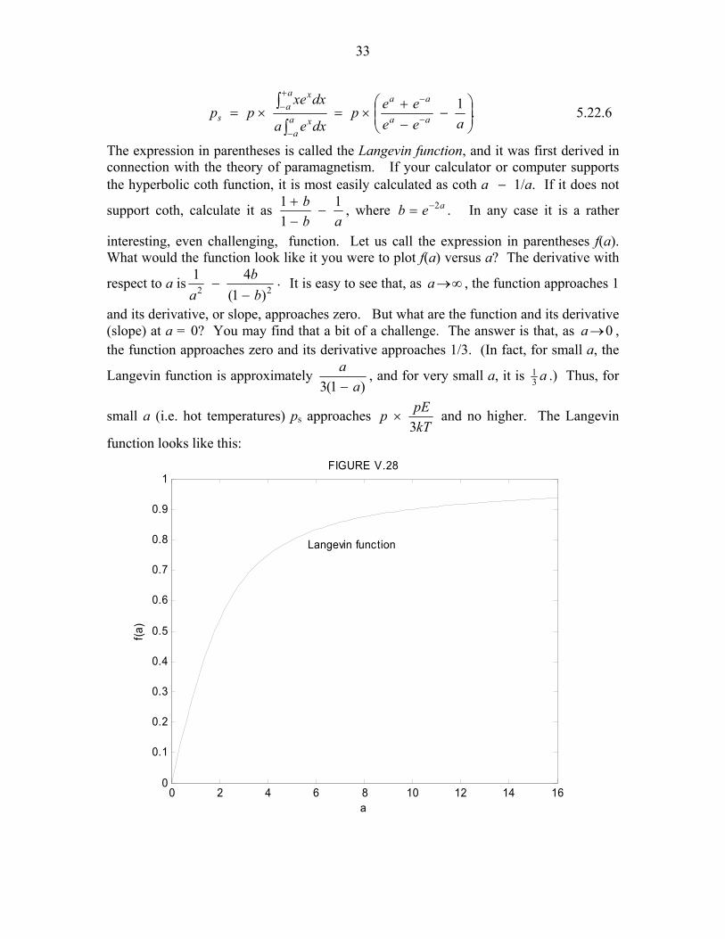
33

.1

−

−+

×=×= −

−

−

+−

∫

∫aee

eepdxea

dxxepp aa

aa

aa

x

aa

x

s 5.22.6

The expression in parentheses is called the Langevin function, and it was first derived in connection with the theory of paramagnetism. If your calculator or computer supports the hyperbolic coth function, it is most easily calculated as coth a − 1/a. If it does not

support coth, calculate it as ab

b 111

−−+ , where aeb 2−= . In any case it is a rather

interesting, even challenging, function. Let us call the expression in parentheses f(a). What would the function look like it you were to plot f(a) versus a? The derivative with

respect to a is .)1(

4122 b

ba −

− It is easy to see that, as ∞→a , the function approaches 1

and its derivative, or slope, approaches zero. But what are the function and its derivative (slope) at a = 0? You may find that a bit of a challenge. The answer is that, as 0→a , the function approaches zero and its derivative approaches 1/3. (In fact, for small a, the

Langevin function is approximately )1(3 a

a−

, and for very small a, it is a31 .) Thus, for

small a (i.e. hot temperatures) ps approaches kTpEp

3× and no higher. The Langevin

function looks like this:

0 2 4 6 8 10 12 14 160

0.1

0.2

0.3

0.4

0.5

0.6

0.7

0.8

0.9

1

a

f(a)

Langevin function

FIGURE V.28

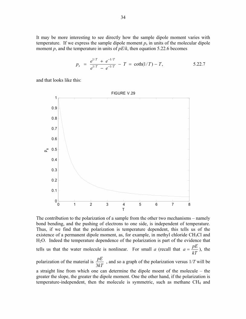
34

It may be more interesting to see directly how the sample dipole moment varies with temperature. If we express the sample dipole moment ps in units of the molecular dipole moment p, and the temperature in units of pE/k, then equation 5.22.6 becomes

,)/1coth(/1/1

/1/1TTT

eeeep TT

TT

s −=−−+

= −

−

5.22.7

and that looks like this:

0 1 2 3 4 5 6 7 80

0.1

0.2

0.3

0.4

0.5

0.6

0.7

0.8

0.9

1

T

p s

FIGURE V.29

The contribution to the polarization of a sample from the other two mechanisms – namely bond bending, and the pushing of electrons to one side, is independent of temperature. Thus, if we find that the polarization is temperature dependent, this tells us of the existence of a permanent dipole moment, as, for example, in methyl chloride CH3Cl and H2O. Indeed the temperature dependence of the polarization is part of the evidence that

tells us that the water molecule is nonlinear. For small a (recall that kTpEa = ), the

polarization of the material is kTpE

3 , and so a graph of the polarization versus 1/T will be

a straight line from which one can determine the dipole moent of the molecule – the greater the slope, the greater the dipole moment. One the other hand, if the polarization is temperature-independent, then the molecule is symmetric, such as methane CH4 and

35

OCO. Indeed the independence of the polarization on temperature is part of the evidence that tells us that CO2 is a linear molecule. 5.22 Dielectric material in a alternating electric field. We have seen that, when we put a dielectric material in an electric field, it becomes polarized, and the D field is now εE instead of merely ε0E. But how long does it take to become polarized? Does it happen instantaneously? In practice there is an enormous range in relaxation times. (We may define a relaxation time as the time taken for the material to reach a certain fraction – such as, perhaps 631 1 =− −e percent, or whatever fraction may be convenient in a particular context – of its final polarization.) The relaxation time may be practically isntantaneous, or it may be many hours. As a consequence of the finite relaxation time, if we put a dielectric material in oscillating electric field tEE ω= cosˆ (e.g. if light passes through a piece of glass), there will be a phase lag of D behind E. D will vary as )cos(ˆ δ−ω= tDD . Stated another way, if the E-field is tieEE ω= ˆ , the D-field will be .ˆ )( δ−ω= tieDD Then

).sin(cosˆˆ

δ−δε== δ− ieED

ED i This can be written

,*ED ε= 5.22.1 where "'* ε−ε=ε i and δε=ε cos' and .sin" δε=ε The complex permittivity is just a way of expressing the phase difference between D and E. The magnitude, or modulus, of *ε is ε, the ordinary permittivity in a static field. Let us imagine that we have a dielectric material between the plates of a capacitor, and that an alternating potential difference is being applied across the plates. At some instant the charge density σ on the plates (which is equal to the D-field) is changing at a rate σ& , which is also equal to the rate of change D& of the D-field), and the current in the circuit is DA & , where A is the area of each plate. The potential difference across the plates, on the other hand, is Ed, where d is the distance between the plates. The instantaneous rate of dissipation of energy in the material is DAdE & , or, let’s say, the instantaneous rate of dissipation of energy per unit volume of the material is DE & . Suppose tEE ω= cosˆ and that )cos(ˆ δ−ω= tDD so that

).sincoscos(sinˆ)sin(ˆ δω−δωω−=δ−ωω−= ttDtDD&

36

The dissipation of energy, in unit volume, in a complete cycle (or period 2π/ω) is the integral, with respect to time, of DE & from 0 to 2π/ω. That is,

.)sincoscos(sincosˆˆ /20 dttttDE δω−δωωω∫

ωπ

The first integral is zero, so the dissipation of energy per unit volume per cycle is

.sinˆˆcossinˆˆ /20

2 δωπ=ωδω ∫ωπ DEdttDE

Since the energy loss per cycle is proportional to sin δ, sin δ is called the loss factor. (Sometimes the loss factor is given as tan δ, although this is an approximation only for small loss angles.)

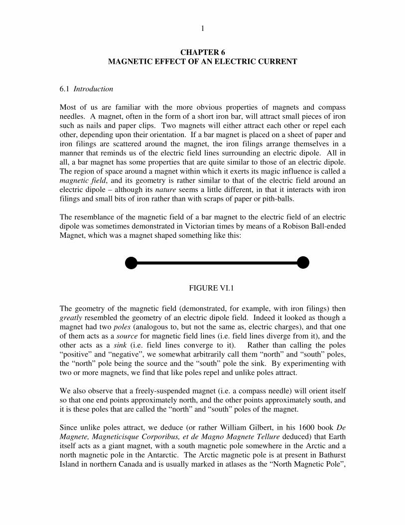
1

CHAPTER 6

MAGNETIC EFFECT OF AN ELECTRIC CURRENT

6.1 Introduction

Most of us are familiar with the more obvious properties of magnets and compass

needles. A magnet, often in the form of a short iron bar, will attract small pieces of iron

such as nails and paper clips. Two magnets will either attract each other or repel each

other, depending upon their orientation. If a bar magnet is placed on a sheet of paper and

iron filings are scattered around the magnet, the iron filings arrange themselves in a

manner that reminds us of the electric field lines surrounding an electric dipole. All in

all, a bar magnet has some properties that are quite similar to those of an electric dipole.

The region of space around a magnet within which it exerts its magic influence is called a

magnetic field, and its geometry is rather similar to that of the electric field around an

electric dipole – although its nature seems a little different, in that it interacts with iron

filings and small bits of iron rather than with scraps of paper or pith-balls.

The resemblance of the magnetic field of a bar magnet to the electric field of an electric

dipole was sometimes demonstrated in Victorian times by means of a Robison Ball-ended

Magnet, which was a magnet shaped something like this:

The geometry of the magnetic field (demonstrated, for example, with iron filings) then

greatly resembled the geometry of an electric dipole field. Indeed it looked as though a

magnet had two poles (analogous to, but not the same as, electric charges), and that one

of them acts as a source for magnetic field lines (i.e. field lines diverge from it), and the

other acts as a sink (i.e. field lines converge to it). Rather than calling the poles

“positive” and “negative”, we somewhat arbitrarily call them “north” and “south” poles,

the “north” pole being the source and the “south” pole the sink. By experimenting with

two or more magnets, we find that like poles repel and unlike poles attract.

We also observe that a freely-suspended magnet (i.e. a compass needle) will orient itself

so that one end points approximately north, and the other points approximately south, and

it is these poles that are called the “north” and “south” poles of the magnet.

Since unlike poles attract, we deduce (or rather William Gilbert, in his 1600 book De

Magnete, Magneticisque Corporibus, et de Magno Magnete Tellure deduced) that Earth

itself acts as a giant magnet, with a south magnetic pole somewhere in the Arctic and a

north magnetic pole in the Antarctic. The Arctic magnetic pole is at present in Bathurst

Island in northern Canada and is usually marked in atlases as the “North Magnetic Pole”,

FIGURE VI.1

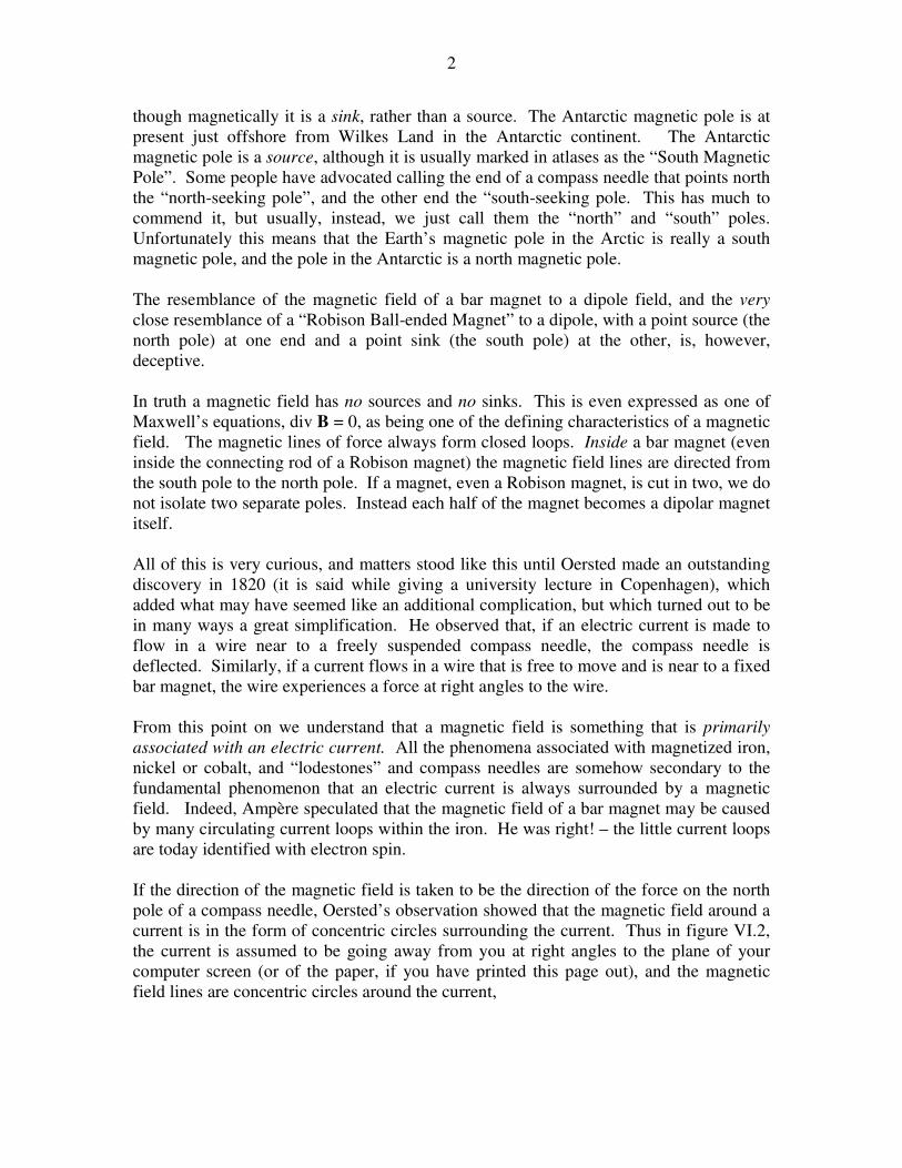
2

though magnetically it is a sink, rather than a source. The Antarctic magnetic pole is at

present just offshore from Wilkes Land in the Antarctic continent. The Antarctic

magnetic pole is a source, although it is usually marked in atlases as the “South Magnetic

Pole”. Some people have advocated calling the end of a compass needle that points north

the “north-seeking pole”, and the other end the “south-seeking pole. This has much to

commend it, but usually, instead, we just call them the “north” and “south” poles.

Unfortunately this means that the Earth’s magnetic pole in the Arctic is really a south

magnetic pole, and the pole in the Antarctic is a north magnetic pole.

The resemblance of the magnetic field of a bar magnet to a dipole field, and the very

close resemblance of a “Robison Ball-ended Magnet” to a dipole, with a point source (the

north pole) at one end and a point sink (the south pole) at the other, is, however,

deceptive.

In truth a magnetic field has no sources and no sinks. This is even expressed as one of

Maxwell’s equations, div B = 0, as being one of the defining characteristics of a magnetic

field. The magnetic lines of force always form closed loops. Inside a bar magnet (even

inside the connecting rod of a Robison magnet) the magnetic field lines are directed from

the south pole to the north pole. If a magnet, even a Robison magnet, is cut in two, we do

not isolate two separate poles. Instead each half of the magnet becomes a dipolar magnet

itself.

All of this is very curious, and matters stood like this until Oersted made an outstanding

discovery in 1820 (it is said while giving a university lecture in Copenhagen), which

added what may have seemed like an additional complication, but which turned out to be

in many ways a great simplification. He observed that, if an electric current is made to

flow in a wire near to a freely suspended compass needle, the compass needle is

deflected. Similarly, if a current flows in a wire that is free to move and is near to a fixed

bar magnet, the wire experiences a force at right angles to the wire.

From this point on we understand that a magnetic field is something that is primarily

associated with an electric current. All the phenomena associated with magnetized iron,

nickel or cobalt, and “lodestones” and compass needles are somehow secondary to the

fundamental phenomenon that an electric current is always surrounded by a magnetic

field. Indeed, Ampère speculated that the magnetic field of a bar magnet may be caused

by many circulating current loops within the iron. He was right! – the little current loops

are today identified with electron spin.

If the direction of the magnetic field is taken to be the direction of the force on the north

pole of a compass needle, Oersted’s observation showed that the magnetic field around a

current is in the form of concentric circles surrounding the current. Thus in figure VI.2,

the current is assumed to be going away from you at right angles to the plane of your

computer screen (or of the paper, if you have printed this page out), and the magnetic

field lines are concentric circles around the current,

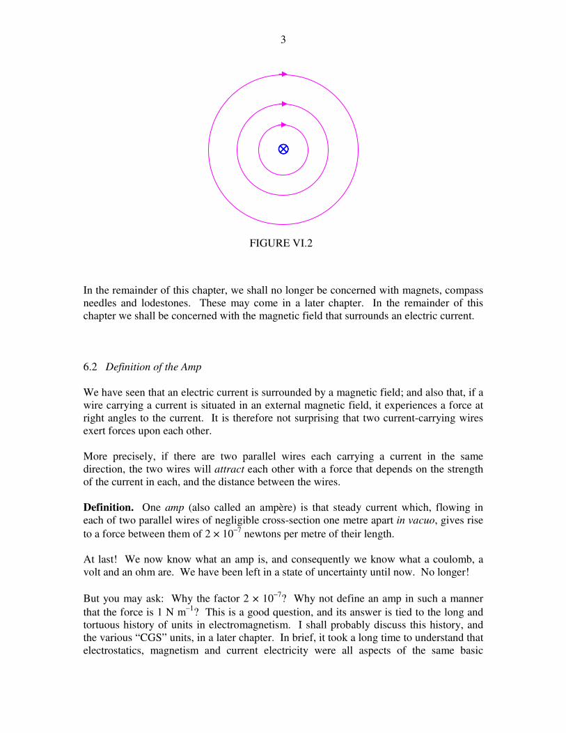
3

In the remainder of this chapter, we shall no longer be concerned with magnets, compass

needles and lodestones. These may come in a later chapter. In the remainder of this

chapter we shall be concerned with the magnetic field that surrounds an electric current.

6.2 Definition of the Amp

We have seen that an electric current is surrounded by a magnetic field; and also that, if a

wire carrying a current is situated in an external magnetic field, it experiences a force at

right angles to the current. It is therefore not surprising that two current-carrying wires

exert forces upon each other.

More precisely, if there are two parallel wires each carrying a current in the same

direction, the two wires will attract each other with a force that depends on the strength

of the current in each, and the distance between the wires.

Definition. One amp (also called an ampère) is that steady current which, flowing in

each of two parallel wires of negligible cross-section one metre apart in vacuo, gives rise

to a force between them of 2 × 10−7

newtons per metre of their length.

At last! We now know what an amp is, and consequently we know what a coulomb, a

volt and an ohm are. We have been left in a state of uncertainty until now. No longer!

But you may ask: Why the factor 2 × 10−7

? Why not define an amp in such a manner

that the force is 1 N m−1

? This is a good question, and its answer is tied to the long and

tortuous history of units in electromagnetism. I shall probably discuss this history, and

the various “CGS” units, in a later chapter. In brief, it took a long time to understand that

electrostatics, magnetism and current electricity were all aspects of the same basic

1111

FIGURE VI.2

4

phenomena, and different systems of units developed within each topic. In particular a

so-called “practical” unit, the amp (defined in terms of the rate of deposition of silver

from an electrolytic solution) became so entrenched that it was felt impractical to

abandon it. Consequently when all the various systems of electromagnetic units became

unified in the twentieth century (starting with proposals by Giorgi based on the metre,

kilogram and second (MKS) as long ago as 1895) in the “Système International” (SI), it

was determined that the fundamental unit of current should be identical with what had

always been known as the ampère. (The factor 2, by the way, is not related to their being

two wires in the definition.) The amp is the only SI unit in which any number other than

“one” is incorporated into its definition, and the exception was forced by the desire to

maintain the amp.

[A proposal to be considered (and probably passed) by the Conférence Générale des Poids et Mesures i n

2015 would re-define the coulomb in such a manner that the magnitude of the charge on a single electron is

exactly 1.60217 % 10−19 C.]

One last point before leaving this section. In the opening paragraph I wrote that “It is

therefore not surprising that two current-carrying wires exert forces upon each other.”

Yet when I first learned, as a student, of the mutual attraction of two parallel electric

currents, I was very astonished indeed. The reason why this is astonishing is discussed in

Chapter 15 (Special Relativity) of the Classical Mechanics section of these notes.

6.3 Definition of the Magnetic Field

We are going to define the magnitude and direction of the magnetic field entirely by

reference to its effect upon an electric current, without reference to magnets or

lodestones. We have already noted that, if an electric current flows in a wire in an

externally-imposed magnetic field, it experiences a force at right angles to the wire.

I want you to imagine that there is a magnetic field in this room, originating, perhaps,

from some source outside the room. This need not entail a great deal of imagination, for

there already is such a magnetic field – namely, Earth’s magnetic field. I’ll tell you that

the field within the room is uniform, but I shan’t tell you anything about either its

magnitude or its direction.

You have a straight wire and you can pass a current through it. You will note that there is

a force on the wire. Perhaps we can define the direction of the field as being the direction

of this force. But this won’t do at all, because the force is always at right angles to the

wire no matter what its orientation! We do notice, however, that the magnitude of the

force depends on the orientation of the wire; and there is one unique orientation of the

wire in which it experiences no force at all. Since this orientation is unique, we choose

to define the direction of the magnetic field as being parallel to the wire when the

orientation of the wire is such that it experiences no force.

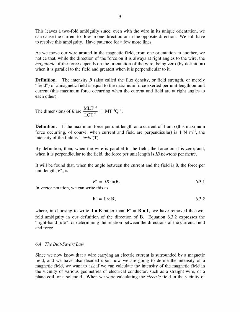
5

This leaves a two-fold ambiguity since, even with the wire in its unique orientation, we

can cause the current to flow in one direction or in the opposite direction. We still have

to resolve this ambiguity. Have patience for a few more lines.

As we move our wire around in the magnetic field, from one orientation to another, we

notice that, while the direction of the force on it is always at right angles to the wire, the

magnitude of the force depends on the orientation of the wire, being zero (by definition)

when it is parallel to the field and greatest when it is perpendicular to it.

Definition. The intensity B (also called the flux density, or field strength, or merely

“field”) of a magnetic field is equal to the maximum force exerted per unit length on unit

current (this maximum force occurring when the current and field are at right angles to

each other).

The dimensions of B are .QMTLQT

MLT 11

1

2−−

−

−

=

Definition. If the maximum force per unit length on a current of 1 amp (this maximum

force occurring, of course, when current and field are perpendicular) is 1 N m−1

, the

intensity of the field is 1 tesla (T).

By definition, then, when the wire is parallel to the field, the force on it is zero; and,

when it is perpendicular to the field, the force per unit length is IB newtons per metre.

It will be found that, when the angle between the current and the field is θ, the force per

unit length, 'F , is

.sin' θ= IBF 6.3.1

In vector notation, we can write this as

,BIF' ××××= 6.3.2

where, in choosing to write BI ×××× rather than ,IBF' ××××= we have removed the two-

fold ambiguity in our definition of the direction of B. Equation 6.3.2 expresses the

“right-hand rule” for determining the relation between the directions of the current, field

and force.

6.4 The Biot-Savart Law

Since we now know that a wire carrying an electric current is surrounded by a magnetic

field, and we have also decided upon how we are going to define the intensity of a

magnetic field, we want to ask if we can calculate the intensity of the magnetic field in

the vicinity of various geometries of electrical conductor, such as a straight wire, or a

plane coil, or a solenoid. When we were calculating the electric field in the vicinity of

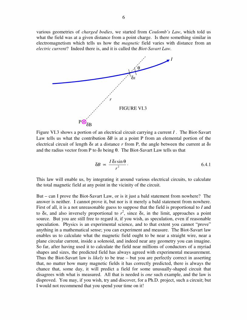
6

various geometries of charged bodies, we started from Coulomb’s Law, which told us

what the field was at a given distance from a point charge. Is there something similar in

electromagnetism which tells us how the magnetic field varies with distance from an

electric current? Indeed there is, and it is called the Biot-Savart Law.

Figure VI.3 shows a portion of an electrical circuit carrying a current I . The Biot-Savart

Law tells us what the contribution δB is at a point P from an elemental portion of the

electrical circuit of length δs at a distance r from P, the angle between the current at δs

and the radius vector from P to δs being θ. The Biot-Savart Law tells us that

.sin2

r

sIB

θδ∝δ 6.4.1

This law will enable us, by integrating it around various electrical circuits, to calculate

the total magnetic field at any point in the vicinity of the circuit.

But – can I prove the Biot-Savart Law, or is it just a bald statement from nowhere? The

answer is neither. I cannot prove it, but nor is it merely a bald statement from nowhere.

First of all, it is a not unreasonable guess to suppose that the field is proportional to I and

to δs, and also inversely proportional to r2, since δs, in the limit, approaches a point

source. But you are still free to regard it, if you wish, as speculation, even if reasonable

speculation. Physics is an experimental science, and to that extent you cannot “prove”

anything in a mathematical sense; you can experiment and measure. The Biot-Savart law

enables us to calculate what the magnetic field ought to be near a straight wire, near a

plane circular current, inside a solenoid, and indeed near any geometry you can imagine.

So far, after having used it to calculate the field near millions of conductors of a myriad

shapes and sizes, the predicted field has always agreed with experimental measurement.

Thus the Biot-Savart law is likely to be true – but you are perfectly correct in asserting

that, no matter how many magnetic fields it has correctly predicted, there is always the

chance that, some day, it will predict a field for some unusually-shaped circuit that

disagrees with what is measured. All that is needed is one such example, and the law is

disproved. You may, if you wish, try and discover, for a Ph.D. project, such a circuit; but

I would not recommend that you spend your time on it!

δs

I

P1111 δB

r

θ

FIGURE VI.3

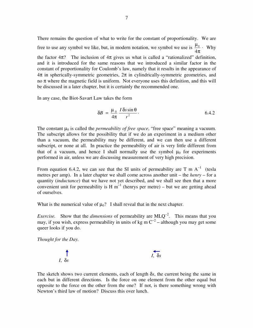
7

There remains the question of what to write for the constant of proportionality. We are

free to use any symbol we like, but, in modern notation, we symbol we use is .4

0

π

µ Why

the factor 4π? The inclusion of 4π gives us what is called a “rationalized” definition,

and it is introduced for the same reasons that we introduced a similar factor in the

constant of proportionality for Coulomb’s law, namely that it results in the appearance of

4π in spherically-symmetric geometries, 2π in cylindrically-symmetric geometries, and

no π where the magnetic field is uniform. Not everyone uses this definition, and this will

be discussed in a later chapter, but it is certainly the recommended one.

In any case, the Biot-Savart Law takes the form

.sin

4 2

0

r

sIB

θδ

π

µ=δ 6.4.2

The constant µ0 is called the permeability of free space, “free space” meaning a vacuum.

The subscript allows for the possibility that if we do an experiment in a medium other

than a vacuum, the permeability may be different, and we can then use a different

subscript, or none at all. In practice the permeability of air is very little different from

that of a vacuum, and hence I shall normally use the symbol µ0 for experiments

performed in air, unless we are discussing measurement of very high precision.

From equation 6.4.2, we can see that the SI units of permeability are T m A−1

(tesla

metres per amp). In a later chapter we shall come across another unit – the henry – for a

quantity (inductance) that we have not yet described, and we shall see then that a more

convenient unit for permeability is H m−1

(henrys per metre) – but we are getting ahead

of ourselves.

What is the numerical value of µ0? I shall reveal that in the next chapter.

Exercise. Show that the dimensions of permeability are MLQ−2

. This means that you

may, if you wish, express permeability in units of kg m C−2

– although you may get some

queer looks if you do.

Thought for the Day.

The sketch shows two current elements, each of length δs, the current being the same in

each but in different directions. Is the force on one element from the other equal but

opposite to the force on the other from the one? If not, is there something wrong with

Newton’s third law of motion? Discuss this over lunch.

I, δs

I, δs

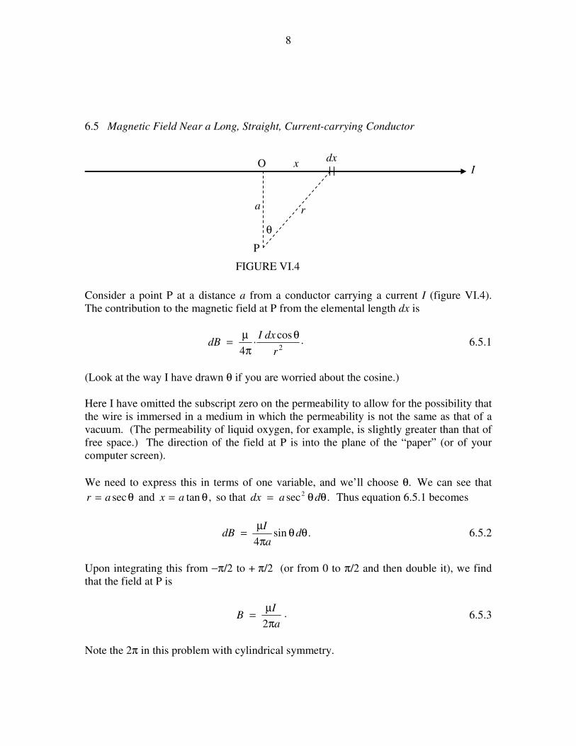
8

6.5 Magnetic Field Near a Long, Straight, Current-carrying Conductor

Consider a point P at a distance a from a conductor carrying a current I (figure VI.4).

The contribution to the magnetic field at P from the elemental length dx is

.cos.

4 2r

dxIdB

θ

π

µ= 6.5.1

(Look at the way I have drawn θ if you are worried about the cosine.)

Here I have omitted the subscript zero on the permeability to allow for the possibility that

the wire is immersed in a medium in which the permeability is not the same as that of a

vacuum. (The permeability of liquid oxygen, for example, is slightly greater than that of

free space.) The direction of the field at P is into the plane of the “paper” (or of your

computer screen).

We need to express this in terms of one variable, and we’ll choose θ. We can see that

θ= secar and ,tan θ= ax so that .sec2 θθ= dadx Thus equation 6.5.1 becomes

.sin4

θθπ

µ= d

a

IdB 6.5.2

Upon integrating this from −π/2 to + π/2 (or from 0 to π/2 and then double it), we find

that the field at P is

.2 a

IB

π

µ= 6.5.3

Note the 2π in this problem with cylindrical symmetry.

P

O

a

dx x

θ

r

FIGURE VI.4

I

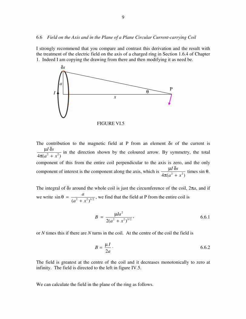
9

6.6 Field on the Axis and in the Plane of a Plane Circular Current-carrying Coil

I strongly recommend that you compare and contrast this derivation and the result with

the treatment of the electric field on the axis of a charged ring in Section 1.6.4 of Chapter

1. Indeed I am copying the drawing from there and then modifying it as need be.

The contribution to the magnetic field at P from an element δs of the current is

)(4 22xa

sI

+π

δµin the direction shown by the coloured arrow. By symmetry, the total

component of this from the entire coil perpendicular to the axis is zero, and the only

component of interest is the component along the axis, which is )(4 22

xa

sI

+π

δµtimes sin θ.

The integral of δs around the whole coil is just the circumference of the coil, 2πa, and if

we write 2/122 )(

sinxa

a

+=θ , we find that the field at P from the entire coil is

,)(2 2/322

2

xa

IaB

+

µ= 6.6.1

or N times this if there are N turns in the coil. At the centre of the coil the field is

.2a

IB

µ= 6.6.2

The field is greatest at the centre of the coil and it decreases monotonically to zero at

infinity. The field is directed to the left in figure IV.5.

We can calculate the field in the plane of the ring as follows.

a

x

δs

θ P

FIGURE VI.5

I

10

Consider an element of the wire at Q of length φad . The angle between the current at Q

and the line PQ is 90º − (θ − φ). The contribution to the B-field at P from the current I

this element is

.)cos(.

4 2

0

r

dIa φφ−θ

π

µ

The field from the entire ring is therefore

θ φ

O P

Q

x

r

a

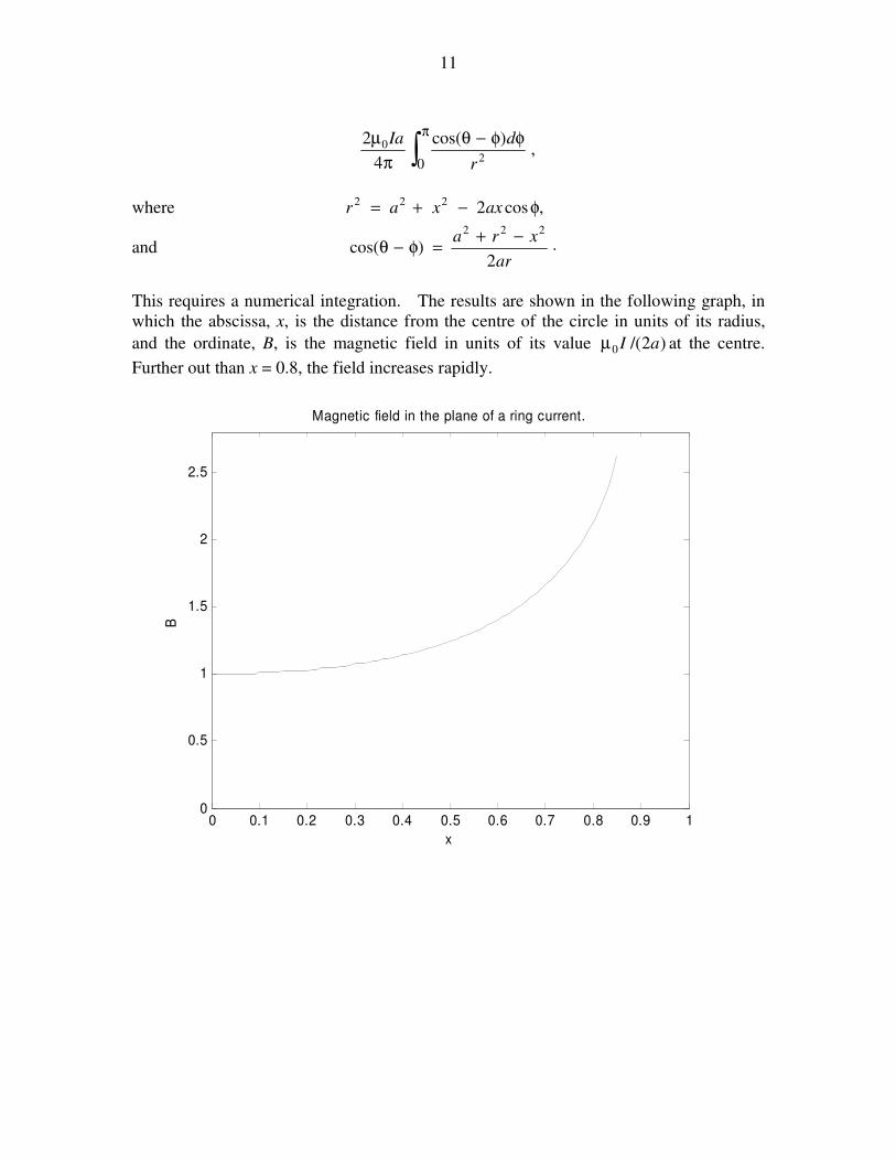
11

,)cos(

4

22

0

0 r

dIa φφ−θ

π

µ π

∫

where ,cos2222 φ−+= axxar

and .2

)cos(222

ar

xra −+=φ−θ

This requires a numerical integration. The results are shown in the following graph, in

which the abscissa, x, is the distance from the centre of the circle in units of its radius,

and the ordinate, B, is the magnetic field in units of its value )2/(0 aIµ at the centre.

Further out than x = 0.8, the field increases rapidly.

0 0.1 0.2 0.3 0.4 0.5 0.6 0.7 0.8 0.9 10

0.5

1

1.5

2

2.5

x

B

Magnetic field in the plane of a ring current.

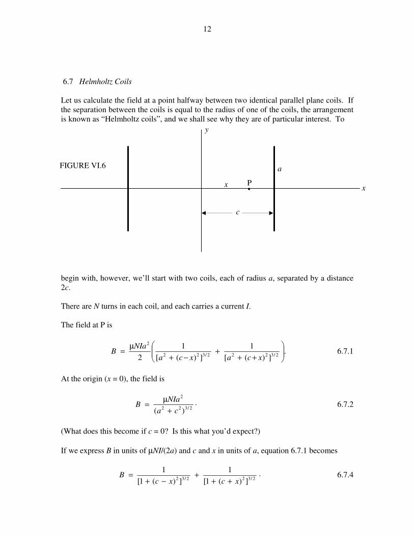
12

6.7 Helmholtz Coils

Let us calculate the field at a point halfway between two identical parallel plane coils. If

the separation between the coils is equal to the radius of one of the coils, the arrangement

is known as “Helmholtz coils”, and we shall see why they are of particular interest. To

begin with, however, we’ll start with two coils, each of radius a, separated by a distance

2c.

There are N turns in each coil, and each carries a current I.

The field at P is

.])([

1

])([

1

2 2/3222/322

2

+++

−+

µ=

xcaxca

NIaB 6.7.1

At the origin (x = 0), the field is

.)( 2/322

2

ca

NIaB

+

µ= 6.7.2

(What does this become if c = 0? Is this what you’d expect?)

If we express B in units of µNI/(2a) and c and x in units of a, equation 6.7.1 becomes

.])(1[

1

])(1[

12/322/32

xcxcB

+++

−+= 6.7.4

x

y

c

a

P

FIGURE VI.6

• x

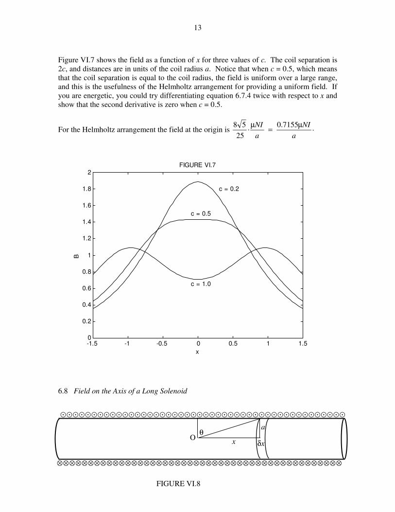
13

Figure VI.7 shows the field as a function of x for three values of c. The coil separation is

2c, and distances are in units of the coil radius a. Notice that when c = 0.5, which means

that the coil separation is equal to the coil radius, the field is uniform over a large range,

and this is the usefulness of the Helmholtz arrangement for providing a uniform field. If

you are energetic, you could try differentiating equation 6.7.4 twice with respect to x and

show that the second derivative is zero when c = 0.5.

For the Helmholtz arrangement the field at the origin is .7155.0.25

58

a

NI

a

NI µ=

µ

-1.5 -1 -0.5 0 0.5 1 1.50

0.2

0.4

0.6

0.8

1

1.2

1.4

1.6

1.8

2

x

B

FIGURE VI.7

c = 0.2

c = 0.5

c = 1.0

6.8 Field on the Axis of a Long Solenoid

??????????????????????????????????????????????

1111111111111111111111111111111111111111111111

FIGURE VI.8

O x δx

θ a

14

The solenoid, of radius a, is wound with n turns per unit length of a wire carrying a

current in the direction indicated by the symbols 1 and ?. At a point O on the axis of

the solenoid the contribution to the magnetic field arising from an elemental ring of width

δx (hence having n δx turns) at a distance x from O is

.)(

.2)(2 2/322

3

2/322

2

xa

xa

a

nI

xa

aIxnB

+

δµ=

+

δµ=δ 6.8.1

This field is directed towards the right.

Let us express this in terms of the angle θ.

We have .cos)(

and,sec,tan 3

2/322

32 θ=

+δθθ=δθ=

xa

aaxax Equation 6.8.1

becomes

.cos21 θµ=δ nIB 6.8.2

If the solenoid is of infinite length, to find the field from the entire infinite solenoid, we

integrate from θ = π/2 to 0 and double it. Thus

∫π

θθµ=2/

0.cos dnIB 6.8.3

Thus the field on the axis of the solenoid is

.nIB µ= 6.8.4

This is the field on the axis of the solenoid. What happens if we move away from the

axis? Is the field a little greater as we move away from the axis, or is it a little less? Is

the field a maximum on the axis, or a minimum? Or does the field go through a

maximum, or a minimum, somewhere between the axis and the circumference? We shall

answer these questions in section 6.11.

6.9 The Magnetic Field H

If you look at the various formulas for the magnetic field B near various geometries of

conductor, such as equations 6.5.3, 6.6.2, 6.7.1, 6.8.4, you will see that there is always a

µ on the right hand side. It is often convenient to define a quantity H = B/µ. Then these

equations become just

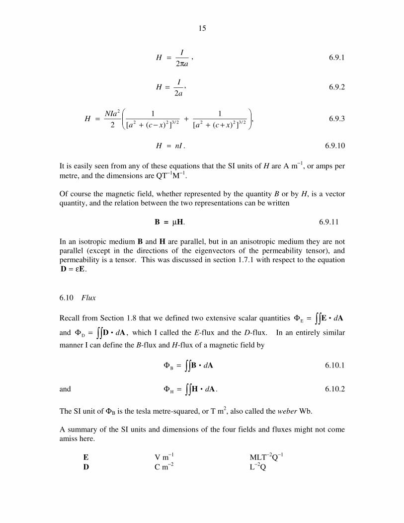
15

,2 a

IH

π= 6.9.1

,2a

IH = 6.9.2

,])([

1

])([

1

2 2/3222/322

2

+++

−+=

xcaxca

NIaH 6.9.3

.nIH = 6.9.10

It is easily seen from any of these equations that the SI units of H are A m−1

, or amps per

metre, and the dimensions are QT−1

M−1

.

Of course the magnetic field, whether represented by the quantity B or by H, is a vector

quantity, and the relation between the two representations can be written

B = µH. 6.9.11

In an isotropic medium B and H are parallel, but in an anisotropic medium they are not

parallel (except in the directions of the eigenvectors of the permeability tensor), and

permeability is a tensor. This was discussed in section 1.7.1 with respect to the equation

.ED ε=

6.10 Flux

Recall from Section 1.8 that we defined two extensive scalar quantities ∫∫ •=Φ AE dE

and ,D ∫∫ •=Φ AD d which I called the E-flux and the D-flux. In an entirely similar

manner I can define the B-flux and H-flux of a magnetic field by

∫∫ •=Φ AB dB 6.10.1

and .H ∫∫ •=Φ AH d 6.10.2

The SI unit of ΦB is the tesla metre-squared, or T m2, also called the weber Wb.

A summary of the SI units and dimensions of the four fields and fluxes might not come

amiss here.

E V m−1

MLT−2

Q−1

D C m−2

L−2

Q

16

B T MT−1

Q−1

H A m−1

L−1

T−1

Q

ΦE V m ML3T

−2Q

−1

ΦD C Q

ΦB Wb ML2T

−1Q

−1

ΦH A m LT−1

Q

6.11 Ampère’s Theorem

In Section 1.9 we introduced Gauss’s theorem, which is that the total normal component

of the D-flux through a closed surface is equal to the charge enclosed within that surface.

Gauss’s theorem is a consequence of Coulomb’s law, in which the electric field from a

point source falls off inversely as the square of the distance. We found that Gauss’s

theorem was surprisingly useful in that it enabled us almost immediately to write down

expressions for the electric field in the vicinity of various shapes of charged bodies

without going through a whole lot of calculus.

Is there perhaps a similar theorem concerned with the magnetic field around a current-

carrying conductor that will enable us to calculate the magnetic field in its vicinity

without going through a lot of calculus? There is indeed, and it is called Ampère’s

Theorem.

? I

FIGURE VI.9

δs

H

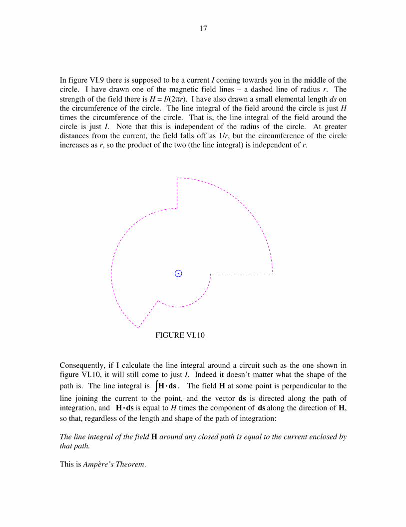
17

In figure VI.9 there is supposed to be a current I coming towards you in the middle of the

circle. I have drawn one of the magnetic field lines – a dashed line of radius r. The

strength of the field there is H = I/(2πr). I have also drawn a small elemental length ds on

the circumference of the circle. The line integral of the field around the circle is just H

times the circumference of the circle. That is, the line integral of the field around the

circle is just I. Note that this is independent of the radius of the circle. At greater

distances from the current, the field falls off as 1/r, but the circumference of the circle

increases as r, so the product of the two (the line integral) is independent of r.

Consequently, if I calculate the line integral around a circuit such as the one shown in

figure VI.10, it will still come to just I. Indeed it doesn’t matter what the shape of the

path is. The line integral is ∫ • dsH . The field H at some point is perpendicular to the

line joining the current to the point, and the vector ds is directed along the path of

integration, and dsH • is equal to H times the component of ds along the direction of H,

so that, regardless of the length and shape of the path of integration:

The line integral of the field H around any closed path is equal to the current enclosed by

that path.

This is Ampère’s Theorem.

?

FIGURE VI.10

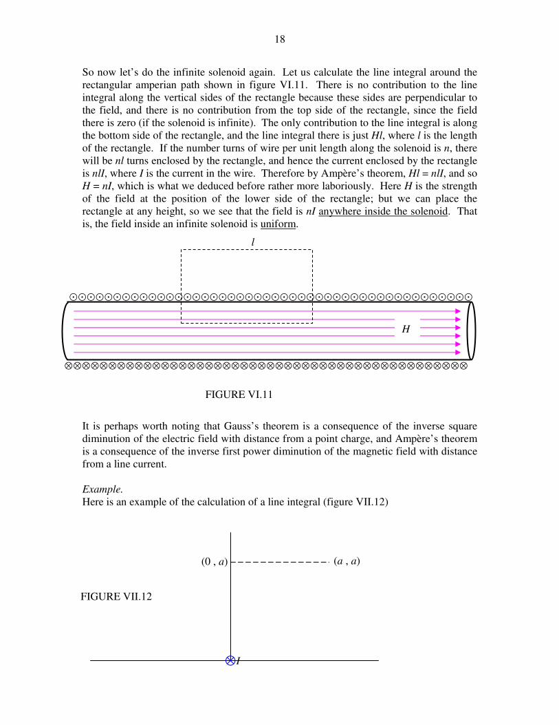
18

So now let’s do the infinite solenoid again. Let us calculate the line integral around the

rectangular amperian path shown in figure VI.11. There is no contribution to the line

integral along the vertical sides of the rectangle because these sides are perpendicular to

the field, and there is no contribution from the top side of the rectangle, since the field

there is zero (if the solenoid is infinite). The only contribution to the line integral is along

the bottom side of the rectangle, and the line integral there is just Hl, where l is the length

of the rectangle. If the number turns of wire per unit length along the solenoid is n, there

will be nl turns enclosed by the rectangle, and hence the current enclosed by the rectangle

is nlI, where I is the current in the wire. Therefore by Ampère’s theorem, Hl = nlI, and so

H = nI, which is what we deduced before rather more laboriously. Here H is the strength

of the field at the position of the lower side of the rectangle; but we can place the

rectangle at any height, so we see that the field is nI anywhere inside the solenoid. That

is, the field inside an infinite solenoid is uniform.

It is perhaps worth noting that Gauss’s theorem is a consequence of the inverse square

diminution of the electric field with distance from a point charge, and Ampère’s theorem

is a consequence of the inverse first power diminution of the magnetic field with distance

from a line current.

Example.

Here is an example of the calculation of a line integral (figure VII.12)

??????????????????????????????????????????????

1111111111111111111111111111111111111111111111

FIGURE VI.11

H

l

1I

(a , a) (0 , a)

FIGURE VII.12

19

An electric current I flows into the plane of the paper at the origin of coordinates.

Calculate the line integral of the magnetic field along the straight line joining the points

(0 , a) and (a , a).

In figure VII.13 I draw a (circular) line of force of the magnetic field H, and a vector dx

where the line of force crosses the straight line of interest.

The line integral along the elemental length dx is H . dx = H dx cos θ . Here

2/122 )(2 xa

IH

+π= and

2/122 )(cos

xa

a

+=θ , and so the line integral along dx is

.)(2 22

xa

dxaI

+π Integrate this from x = 0 to x = a and you will find that the answer is I/8.

Figure VII.14 shows another method. The line integral around the square is, by

Ampère’s theorem, I, and so the line integral an eighth of the way round is I/8.

You will probably immediately feel that this second method is much the better and very

“clever”. I do not deny this, but it is still worthwhile to study carefully the process of line

integration in the first method.

1I

(a , a) (0 , a) FIGURE VII.13

H

dx

θ

x

a

20

Another Example

An electric current I flows into the plane of the paper. Calculate the line integral of the

magnetic field along a straight line of length 2a whose mid-point is at a distance 3/a from the current.

1I

(a , a)

FIGURE VII.14

1111I

3/a

a

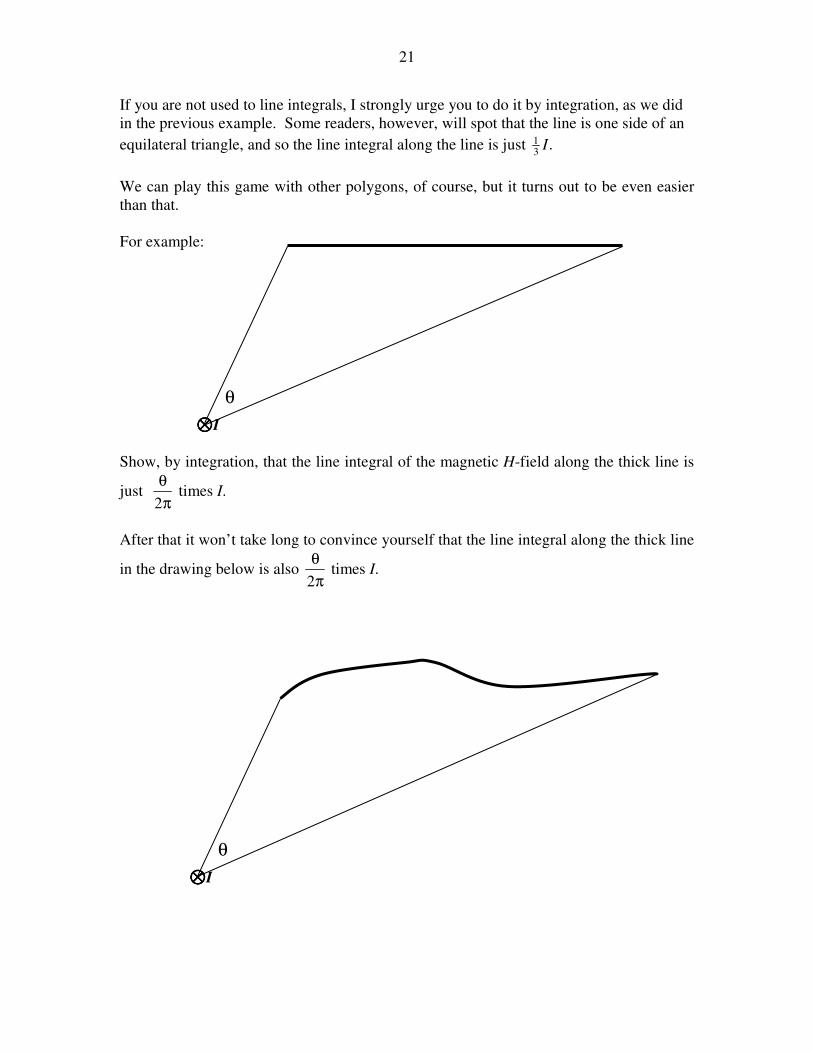
21

If you are not used to line integrals, I strongly urge you to do it by integration, as we did

in the previous example. Some readers, however, will spot that the line is one side of an

equilateral triangle, and so the line integral along the line is just .31

I

We can play this game with other polygons, of course, but it turns out to be even easier

than that.

For example:

Show, by integration, that the line integral of the magnetic H-field along the thick line is

just π

θ

2 times I.

After that it won’t take long to convince yourself that the line integral along the thick line

in the drawing below is also π

θ

2 times I.

1111I

θ

1111I

θ

22

Another Example

A straight cylindrical metal rod (or a wire for that matter) of radius a carries a current I.

At a distance r from the axis, the magnetic field is clearly I/(2πr) if r > a. But what is

the magnetic field inside the rod at a distance r from the axis, r < a?

Figure VII.15 shows the cross-section of the rod, and I have drawn an amperian circle of

radius r. If the field at the circumference of the circle is H, the line integral around the

circle is 2πrH. The current enclosed within the circle is Ir2/a

2. These two are equal, and

therefore H = Ir/(2πa2).

More and More Examples

In the above example, the current density was uniform. But now we can think of lots and

lots of examples in which the current density is not uniform. For example, let us

imagine that we have a long straight hollow cylindrical tube of radius a, perhaps a linear

particle accelerator, and the current density J (amps per square metre) varies from the

middle (axis) of the cylinder to its edge according to )./1()( 0 arJrJ −= The total

current is, of course, ,)(2 02

31

0JardrrJI

a

π=π= ∫ and the mean current density is

031

JJ = .

The question, however, is: what is the magnetic field H at a distance r from the axis?

Further, show that the magnetic field at the edge (circumference) of the cylinder is aJ061 ,

and that the field reaches a maximum value of aJ0163 at .

43

ar =

Well, the current enclosed within a distance r from the axis is

),1()(2322

00 a

rr

rJxdxxJI −π=π= ∫

FIGURE VII.15

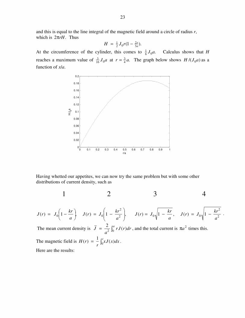
23

and this is equal to the line integral of the magnetic field around a circle of radius r,

which is .2 rHπ Thus

).1(32

021

a

rrJH −=

At the circumference of the cylinder, this comes to .061

aJ Calculus shows that H

reaches a maximum value of aJ0163 at .

43

ar = The graph below shows )/( 0aJH as a

function of x/a.

0 0.1 0.2 0.3 0.4 0.5 0.6 0.7 0.8 0.9 10

0.02

0.04

0.06

0.08

0.1

0.12

0.14

0.16

0.18

0.2

r/a

H/J

0a

Having whetted our appetites, we can now try the same problem but with some other

distributions of current density, such as

.1)(,1)(,1)(,1)(2

2

002

2

00

4321

a

krJrJ

a

krJrJ

a

krJrJ

a

krJrJ −=−=

−=

−=

The mean current density is ∫=a

drrJr

a

J02

)(2

, and the total current is 2aπ times this.

The magnetic field is ∫=r

dxxJxr

rH0

)(1

)( .

Here are the results:

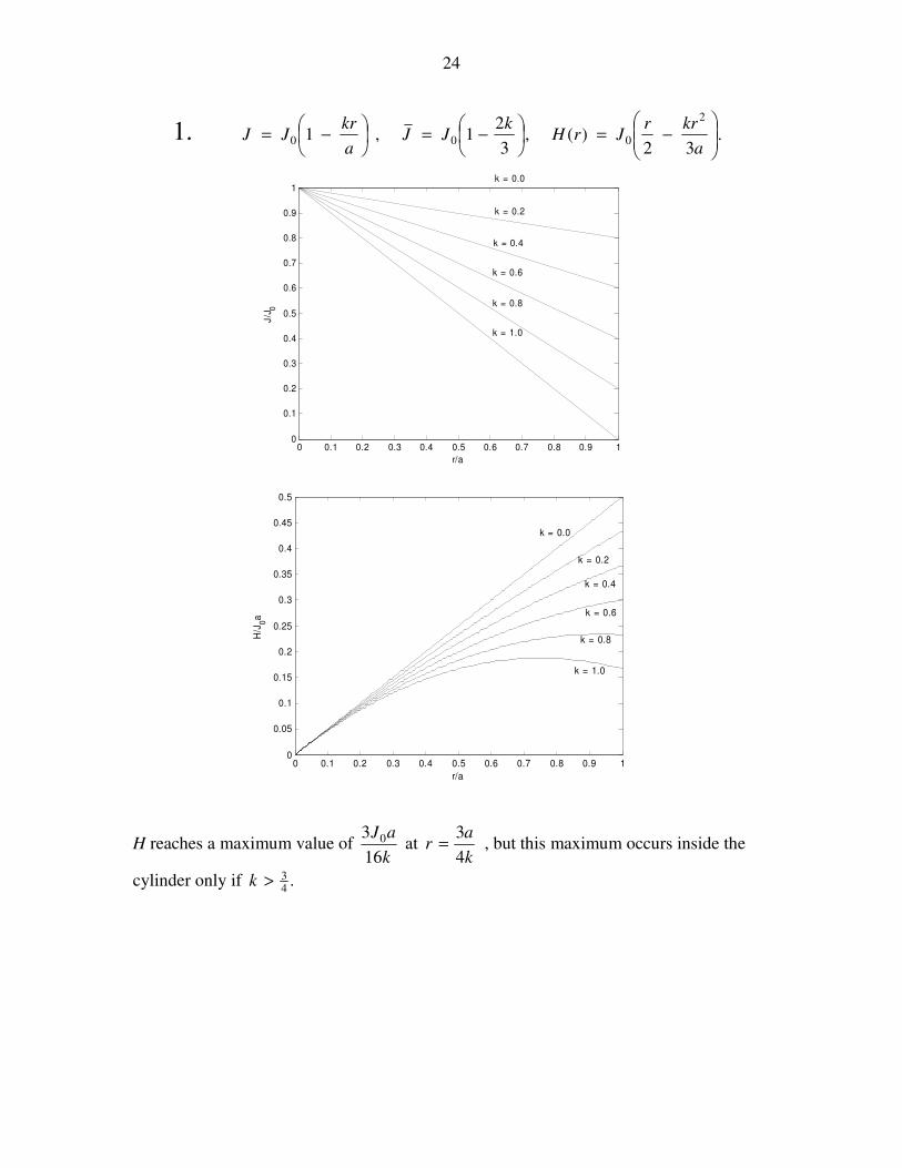
24

1. .32

)(,3

21,1

2

000

−=

−=

−=

a

krrJrH

kJJ

a

krJJ

0 0.1 0.2 0.3 0.4 0.5 0.6 0.7 0.8 0.9 10

0.1

0.2

0.3

0.4

0.5

0.6

0.7

0.8

0.9

1

r/a

J/J

0

k = 0.0

k = 0.2

k = 0.4

k = 0.6

k = 0.8

k = 1.0

0 0.1 0.2 0.3 0.4 0.5 0.6 0.7 0.8 0.9 10

0.05

0.1

0.15

0.2

0.25

0.3

0.35

0.4

0.45

0.5

r/a

H/J

0a

k = 0.0

k = 0.2

k = 0.4

k = 0.6

k = 0.8

k = 1.0

H reaches a maximum value of k

aJ

16

3 0 at k

ar

4

3= , but this maximum occurs inside the

cylinder only if .43>k

25

2. ( ) .42

)(,1,12

3

021

02

2

0

−=−=

−=

a

krrJrHkJJ

a

krJJ

0 0.1 0.2 0.3 0.4 0.5 0.6 0.7 0.8 0.9 10

0.1

0.2

0.3

0.4

0.5

0.6

0.7

0.8

0.9

1

r/a

J/J

0

k = 0.0

k = 0.2

k = 0.4

k = 0.6

k = 0.8

k = 1.0

0 0.1 0.2 0.3 0.4 0.5 0.6 0.7 0.8 0.9 10

0.05

0.1

0.15

0.2

0.25

0.3

0.35

0.4

0.45

0.5

r/a

H/J

0a

k = 0.0

k = 0.2

k = 0.4

k = 0.6

k = 0.8

k = 1.0

H reaches a maximum value of aJk

027

2 at

ka

r

3

2= , but this maximum occurs inside

the cylinder only if .32>k

26

3.

[ ]

.1315215

2)(

,)1(12)1(20815

,1

2/52/3

2

20

2/52/3

2

00

−+

−−=

−+−−=−=

a

kr

a

kr

rk

aJrH

kk

k

JJ

a

krJJ

0 0.1 0.2 0.3 0.4 0.5 0.6 0.7 0.8 0.9 10

0.1

0.2

0.3

0.4

0.5

0.6

0.7

0.8

0.9

1

r/a

J/J

0k = 0.0

k = 0.2

k = 0.4

k = 0.6

k = 0.8

k = 1.0

0 0.1 0.2 0.3 0.4 0.5 0.6 0.7 0.8 0.9 10

0.05

0.1

0.15

0.2

0.25

0.3

0.35

0.4

0.45

0.5

r/a

H/J

0a

k = 0.0

k = 0.2

k = 0.4

k = 0.6

k = 0.8

k = 1.0

I have not calculated explicit formulas for the positions and values of the maxima.

A maximum occurs inside the cylinder if k > 0.908901.

27

4.

[ ]

.113

)(

,)1(13

2,1

2/3

2

220

2/30

2

2

0

−−=

−−=−=

a

kr

kr

aJrH

kk

JJ

a

krJJ

0 0.1 0.2 0.3 0.4 0.5 0.6 0.7 0.8 0.9 10

0.1

0.2

0.3

0.4

0.5

0.6

0.7

0.8

0.9

1

r/a

J/J

0

k = 0.0

k = 0.2

k = 0.4

k = 0.6

k = 0.8

k = 1.0

0 0.1 0.2 0.3 0.4 0.5 0.6 0.7 0.8 0.9 10

0.05

0.1

0.15

0.2

0.25

0.3

0.35

0.4

0.45

0.5

r/a

J/J

0

k = 0.0

k = 0.2

k = 0.4

k = 0.6

k = 0.8

k = 1.0

A maximum occurs inside the cylinder if k > 0.866025.

In all of these cases, the condition that there shall be no maximum H inside the cylinder

– that is, between r = 0 and r = a − is that .2

1)(>

J

aJ I believe this to be true for any

axially symmetric current density distribution, though I have not proved it. I expect that

a fairly simple proof could be found by someone interested.

28

Additional current density distributions that readers might like to investigate are

22 /0

/0

22

0

0

22

00

/1

/1/1/1

axaxeJJeJJ

ax

JJ

ax

JJ

ax

JJ

ax

JJ

−− ==+

=

+=

+=

+=

CHAPTER 7

FORCE ON A CURRENT IN A MAGNETIC FIELD

7.1 Introduction

In Chapter 6 we showed that when an electric current is situated in an external magnetic

field it experiences a force at right angles to both the current and the field. Indeed we

used this to define both the magnitude and direction of the magnetic field. The magnetic

field is defined in magnitude and direction such that the force per unit length F' on the

current is given by

.BIF' ××××= 1.7.1

7.2 Force Between Two Current-carrying Wires

In figure VII.1, we have two parallel currents, I1 and I2, each directed away from you (i.e.

into the plane of the paper) and a distance r apart. The current I1 produces a magnetic

field at I2, directed downward as shown, and of magnitude ),2/(1 rIB πµ= where µ is the

permeability of the medium in which the two wires are immersed. Therefore, following

equation 7.1.1, I2 experiences a force per unit length towards the left ).2/(' 21 rIIF πµ=

You must also go through the same argument to show that the force per unit length on I1

from the magnetic field produced by I2 is of the same magnitude but directed towards the

right, thus satisfying Newton’s third law of motion.

Thus the force of attraction per unit length between two parallel currents a distance r

apart is

.2

' 21

r

IIF

π

µ= 7.2.1

I2

B1

1 1 I1

r

FIGURE VII.1

7.3 The Permeability of Free Space

If each of the currents in the arrangement of Section 7.2 is one amp, and if the distance r

between to two wires is one metre, and if the experiment is performed in a vacuum, so

that µ = µ0, then the force per unit length between the two wires is µ0/(2π) newtons per

metre. But we have already (in Chapter 6) defined the amp in such a manner that this

force is 2 × 10−7

N m−1

. Therefore it follows from our definition of the amp that the

permeability of free space, by definition, has a value of exactly

,AmT104 17

0

−−×π=µ 7.3.1

or, as we shall learn to express it in a later chapter, 7104 −×π henrys per metre, H m−1

.

[It was mentioned briefly in Chapters 1 and 6 that there is a proposal , likely to become official in 2015, to

re-define the coulomb (and hence the amp) in such a manner that the magnitude of the charge on a single

electron is exactly 1.60217 % 10−19 C. If this proposal is passed (as is likely), µ0 will no longer have a

defined value, but will have a measured value of approximately 12.5664 % 10−7

T m A−1

.]

7.4 Magnetic Moment

If a compass needle, or indeed any bar magnet, is placed in an external magnetic field, it

experiences a torque – the one exception being if the needle is placed exactly along the

direction of the field. The torque is greatest when the needle is oriented at right angles to

the field.

Definition. The magnetic moment of a magnet is equal to the maximum torque it

experiences when in unit magnetic field.

As already noted this maximum torque is experienced when the magnet is at right angles

to the magnetic field. In SI units, "unit magnetic field" means, of course, one tesla, and

the SI units of magnetic moment are N m T−1

, or newton metres per tesla. The reader

should look up (or deduce) the dimension of magnetic field (teslas) and then show that

the dimensions of magnetic moment are L2 T

−1Q.

It is noted here that many different definitions of and units for magnetic moment are to be found in the

literature, not all of which are correct or even have the correct dimensions. This will be discussed in a later

chapter. In the meantime the definition we have given above is standard in the Système International.

7.5 Magnetic moment of a Plane, Current-carrying Coil

A plane, current carrying coil also experiences a torque in an external magnetic field, and

its behaviour in a magnetic field is quite similar to that of a bar magnet or a compass

needle. The torque is maximum when the normal to the coil is perpendicular to the

magnetic field, and the magnetic moment is defined in exactly the same way, namely the

maximum torque experienced in unit magnetic field.

Let us examine the behaviour of a rectangular coil of sides a and b, which is free to rotate

about the dashed line shown in figure VII.2.

In figure VII.3 I am looking down the axis represented by the dashed line in figure VII.2,

and we see the coil sideways on. A current I is flowing around the coil in the directions

indicated by the symbols ? and 1. The normal to the coil makes an angle θ with respect

to an external field B.

According to the Biot-Savart law there is a force F on each of the b-length arms of

magnitude bIB, or, if there are N turns in the coil, F = NbIB. These two forces are

opposite in direction and constitute a couple. The perpendicular distance between the

two forces is a sin θ, so the torque τ on the coil is NabIB sin θ, or τ = NAIB sin θ, where

A is the area of the coil. This has its greatest value when θ = 90o, and so the magnetic

FIGURE VII.2

a

b

1

?

FIGURE VII.3

a

θ

F

F

B

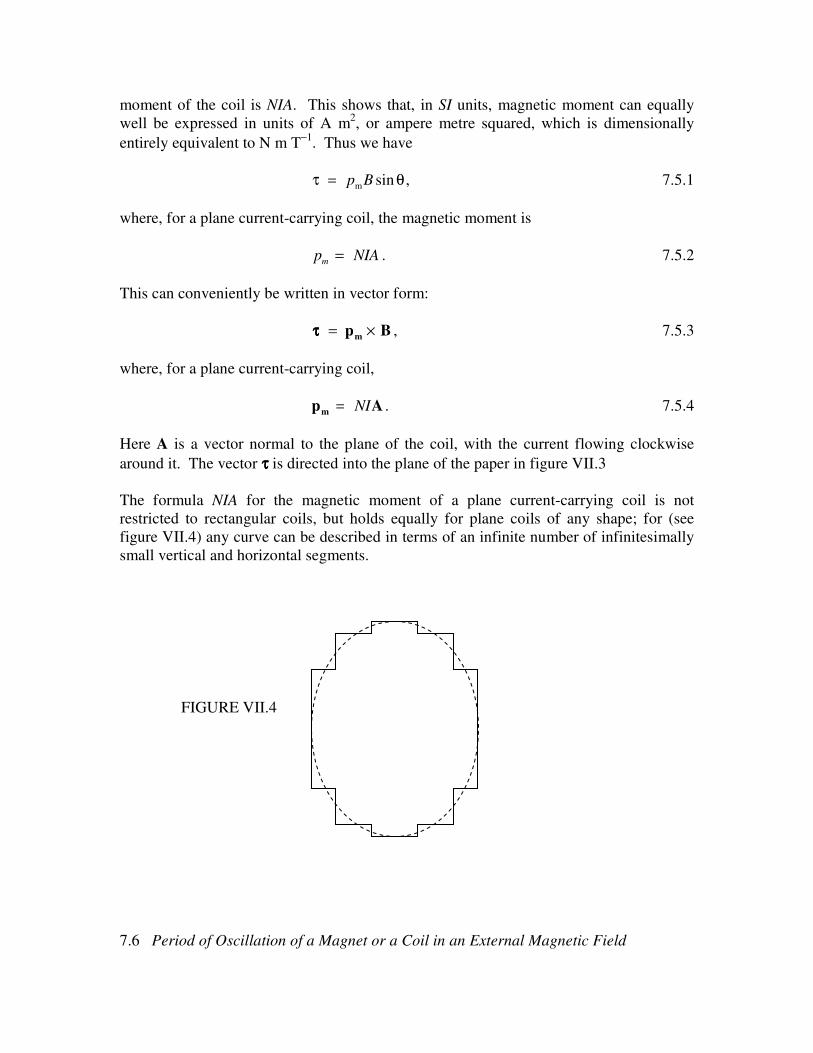
moment of the coil is NIA. This shows that, in SI units, magnetic moment can equally

well be expressed in units of A m2, or ampere metre squared, which is dimensionally

entirely equivalent to N m T−1

. Thus we have

τ θ= p Bm sin , 7.5.1

where, for a plane current-carrying coil, the magnetic moment is

p NIAm

= . 7.5.2

This can conveniently be written in vector form:

ττττ = ×p Bm

, 7.5.3

where, for a plane current-carrying coil,

p Am

= NI . 7.5.4

Here A is a vector normal to the plane of the coil, with the current flowing clockwise

around it. The vector ττττ is directed into the plane of the paper in figure VII.3

The formula NIA for the magnetic moment of a plane current-carrying coil is not

restricted to rectangular coils, but holds equally for plane coils of any shape; for (see

figure VII.4) any curve can be described in terms of an infinite number of infinitesimally

small vertical and horizontal segments.

7.6 Period of Oscillation of a Magnet or a Coil in an External Magnetic Field

FIGURE VII.4

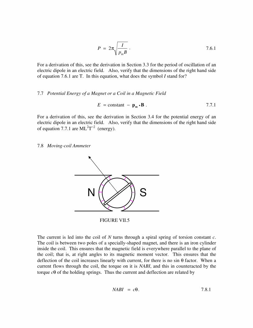
PI

p B= 2π

m

. 7.6.1

For a derivation of this, see the derivation in Section 3.3 for the period of oscillation of an

electric dipole in an electric field. Also, verify that the dimensions of the right hand side

of equation 7.6.1 are T. In this equation, what does the symbol I stand for?

7.7 Potential Energy of a Magnet or a Coil in a Magnetic Field

E = − •constant p Bm

. 7.7.1

For a derivation of this, see the derivation in Section 3.4 for the potential energy of an

electric dipole in an electric field. Also, verify that the dimensions of the right hand side

of equation 7.7.1 are ML2T

−2 (energy).

7.8 Moving-coil Ammeter

The current is led into the coil of N turns through a spiral spring of torsion constant c.

The coil is between two poles of a specially-shaped magnet, and there is an iron cylinder

inside the coil. This ensures that the magnetic field is everywhere parallel to the plane of

the coil; that is, at right angles to its magnetic moment vector. This ensures that the

deflection of the coil increases linearly with current, for there is no sin θ factor. When a

current flows through the coil, the torque on it is NABI, and this in counteracted by the

torque cθ of the holding springs. Thus the current and deflection are related by

NABI c= θ . 7.8.1

S N

FIGURE VII.5

7.9 Magnetogyric Ratio

The magnetic moment and the angular momentum are both important properties of

subatomic particles. Each of them, however, depends on the angular speed of rotation of

the particle. The ratio of magnetic moment to angular momentum, on the other hand, is

independent of the speed of rotation, and tells us something about how the mass and

charge are distributed within the particle. Also, it can be measured with higher precision

than either the magnetic moment or the angular momentum separately. This ratio is

called the magnetogyric ratio (or, perversely and illogically, by some, the "gyromagnetic

ratio"). You should be able to show that the dimensions of the magnetogyric ratio are

QM−1

, and therefore the SI unit is C kg−1

. I doubt, however, if many particle physicists

use such simple units. They probably express magnetic moment in Bohr magnetons or

nuclear magnetons and angular momentum in units of Planck's constant divided by 2π −

but that is not our problem.

Let us calculate the magnetogyric ratio of a point charge and point mass moving in a

circular orbit – rather like the electron moving around the proton in the simplest model of

a hydrogen atom. We'll suppose that the angular speed in the orbit is ω and the radius of

the orbit is a. The angular momentum is easy – it is just ma2ω. The frequency with

which the particle (whose charge is Q) passes a given point in its orbit is ω/(2π), so the

current is Qω/(2π). The area of the orbit is πa2 and so the magnetic moment of the

orbiting particle is 12

2Q aω . The magnetogyric ratio is therefore Q/(2m).

The magnetogyric ratio will be the same as this in any spinning body in which the

distributions of mass density and charge density inside the body are the same. Consider,

however, the magnetogyric ratio of a charged, spinning metal sphere. The mass is

distributed uniformly throughout the sphere, but the charge all resides on the surface. We

may then expect the magnetogyric ratio to be rather larger than q/(2m).

The angular momentum is easy. It is just 25

2ma ω. Now for the magnetic moment. Refer

to figure VII.6.

FIGURE VII.6 θ

a sin θ

ωωωω

The area of the elemental zone shown is 2πa2 sin θ dθ. The area of the entire sphere is

4 2πa , so the charge on the elemental zone is 12

Q dsin .θ θ The zone is spinning, as is the

entire sphere, at an angular speed ω, so the current is

12

24

Q dQ d

sin /( )sin .θ θ ω π

ω θ θ

π× = 7.9.1

The area enclosed by the elemental zone is π θa2 2sin . The magnetic moment dpm of the

zone is the current times the area enclosed, which is

dp Q a dm

= 14

2 3ω θ θsin . 7.9.2

The magnetic moment of the entire sphere is found by integrating this from θ = 0 to π,

whence

p Q am

= 13

2ω . 7.9.3

The ratio of the magnetic moment to the angular momentum is therefore 5Q/(6m).

Those who are familiar with gyroscopic motion will know that if a spinning body of

angular momentum L is subject to a torque ττττ, the angular momentum vector will not be

constant in direction and indeed the rate of change of angular momentum will be equal to

τ. τ. τ. τ. Figure VII.7 is a reminder of the motion of a top in regular precession (that is, with no

nutation).

L

θ

l

FIGURE VII.7

ττττ

Ω

A study of Chapter 4 Section 4.10 of Classical Mechanics will be needed for a more

detailed understanding of the motion of a top. The top is subject to a torque of magnitude

mgl sinθ . The torque can be represented by a vector ττττ directed into the plane of the

paper. As drawn, the angular momentum vector L makes an angle θ with the

gravitational field g, and it precesses about the vertical with an angular velocity ΩΩΩΩ, the

three vectors ττττ, L and ΩΩΩΩ being related by ττττ = L %%%% ΩΩΩΩ. The magnitude of the angular

momentum vector is therefore τ/(L sin θ). But τ = mgl sin θ, so that the precessional

frequency is mgl/L, independent of θ. Likewise a charged spinning body with a

magnetic moment of pm is a magnetic field B experiences a torque ττττ = pm %%%% B, which is

of magnitude pmB sin θ, and consequently its angular momentum vector precesses around

B at an angular speed p

LB

m , independent of θ. (Verify that this has dimensions T−1

.) The

coefficient of B here is the magnetogyric ratio. The precessional speed can be measured

very precisely, and hence the magnetogyric ratio can be measured correspondingly

precisely. This phenomenon of "Larmor precession" is the basis of many interesting

instruments and disciplines, such as the proton precession magnetometer, nuclear

magnetic resonance spectroscopy and nuclear magnetic resonance imaging used in

medicine. Because anything including the word "nuclear" is a politically incorrect

phrase, the word "nuclear” is usually dropped, and nuclear magnetic resonance imaging

is usually called just "magnetic resonance imaging", or MRI, which doesn't quite make

sense, but at least is politically correct.

1CHAPTER 8

ON THE ELECTRODYNAMICS OF MOVING BODIES

1. Introduction First, I have shamelessly plagiarized the title of this chapter. I have stolen the title from that of one of the most famous physics research papers of the twentieth century – Zur Elektrodynamik Bewegter Körper, the paper in which Einstein described the Special Theory of Relativity in 1905. I shall be describing the motion of charged particles in electric and magnetic fields, but, unlike Einstein, I shall (unless I state otherwise – which will happen from time to time) be restricting the considerations of this chapter mostly to nonrelativistic speeds – that is to say speeds such that v2/c2 is much smaller than the level of precision one is interested in or can conveniently measure. Some relativistic aspects of electrodynamics are touched upon briefly in Chapter 15 of the Classical Mechanics notes in this series, but, apart from the fact that this chapter and Einstein's paper both deal with the motions of charged bodies in electric and magnetic fields, there will be little else in common. Section 8.2 will deal with the motion of a charged particle in an electric field alone, and Section 8.3 will deal with the motion of a charged particle in a magnetic field alone. Section 8.4 will deal with the motion of a charged particle where both an electric and a magnetic field are present. That section may be a little more difficult than the others and may be omitted on a first reading by less experienced readers. Section 8.5 deals with the motion of a charged particle in a nonuniform magnetic field and is more difficult again. 8.2 Charged Particle in an Electric Field There is really very little that can be said about a charged particle moving at nonrelativistic speeds in an electric field E. The particle, of charge q and mass m, experiences a force qE, and consequently it accelerates at a rate qE/m. If it starts from rest, you can calculate how fast it is moving in time t, what distance it has travelled in time t, and how fast it is moving after it has covered a distance x, by all the usual first-year equations for uniformly accelerated motion in a straight line. If the charge is accelerated through a potential difference V, its loss of potential energy qV will equal its gain in kinetic energy 1

22mv . Thus v = 2qV m/ .

Let us calculate, using this nonrelativistic formula, the speed gained by an electron that is accelerated through 1, 10, 100, 1000, 10000, 100,000 and 1,000,000 volts, given that, for an electron, e/m = 1.7588 % 1011 C kg−1. (The symbol for the electronic charge is usually written e. You might note here that that's a lot of coulombs per kilogram!). We'll also calculate v/c and v2/c2. V volts v m s−1 v/c v2/c2

1 5.931 % 105 1.978 % 10−3 3.914 % 10−6

10 1.876 % 106 6.256 % 10−3 3.914 % 10−5 100 5.931 % 106 1.978 % 10−2 3.914 % 10−4

2 1000 1.876 % 107 6.256 % 10−2 3.914 % 10−3

10000 5.931 % 107 1.978 % 10−1 3.914 % 10−2 100000 1.876 % 108 6.256 % 10−1 3.914 % 10−1

1000000 5.931 % 108 1.978 3.914 We can see that, even working to a modest precision of four significant figures, an electron accelerated through only a few hundred volts is reaching speeds at which v2/c2 is not quite negligible, and for less than a million volts, the electron is already apparently moving faster than light! Therefore for large voltages the formulas of special relativity should be used. Those who are familiar with special relativity (i.e. those who have read Chapter 15 of Classical Mechanics!), will understand that the relativistically correct relation between potential and kinetic energy is qV = (γ − 1)m0c2, and will be able to calculate the speeds correctly as in the following table. Those who are not familiar with relativity may be a bit lost here, but just take it as a warning that particles such as electrons with a very large charge-to-mass ratio rapidly reach speeds at which relativistic formulas need to be used. These figures are given here merely to give some idea of the magnitude of the potential differences that will accelerate an electron up to speeds where the relativistic formulas must be used.

V volts v m s−1 v/c v2/c2

1 5.931 % 105 1.978 % 10−3 3.914 % 10−6

10 1.875 % 106 6.256 % 10−3 3.914 % 10−5 100 5.930 % 106 1.978 % 10−2 3.912 % 10−4 1000 1.873 % 107 6.247 % 10−2 3.903 % 10−3

10000 5.845 % 107 1.950 % 10−1 3.803 % 10−2

100000 1.644 % 108 5.482 % 10−1 3.005 % 10−1

1000000 2.821 % 108 0.941 0.855 If a charged particle is moving at constant speed in the x-direction, and it encounters a region in which there is an electric field in the y-direction (as in the Thomson e/m experiment, for example) it will accelerate in the y-direction while maintaining its constant speed in the x-direction. Consequently it will move in a parabolic trajectory just like a ball thrown in a uniform gravitational field, and all the familiar analysis of a parabolic trajectory will apply, except that instead of an acceleration g, the acceleration will be q/m. 8.3 Charged Particle in a Magnetic Field We already know that an electric current I flowing in a region of space where there exists a magnetic field B will experience a force that is at right angles to both I and B, and the force per unit length, F', is given by F' = I % B , 8.3.1

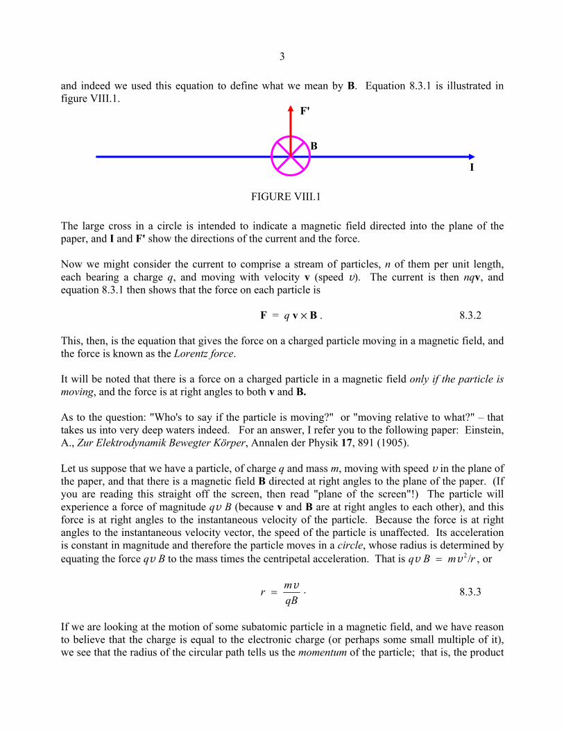
3 and indeed we used this equation to define what we mean by B. Equation 8.3.1 is illustrated in figure VIII.1. The large cross in a circle is intended to indicate a magnetic field directed into the plane of the paper, and I and F' show the directions of the current and the force. Now we might consider the current to comprise a stream of particles, n of them per unit length, each bearing a charge q, and moving with velocity v (speed v). The current is then nqv, and equation 8.3.1 then shows that the force on each particle is F = q v % B . 8.3.2 This, then, is the equation that gives the force on a charged particle moving in a magnetic field, and the force is known as the Lorentz force. It will be noted that there is a force on a charged particle in a magnetic field only if the particle is moving, and the force is at right angles to both v and B. As to the question: "Who's to say if the particle is moving?" or "moving relative to what?" – that takes us into very deep waters indeed. For an answer, I refer you to the following paper: Einstein, A., Zur Elektrodynamik Bewegter Körper, Annalen der Physik 17, 891 (1905). Let us suppose that we have a particle, of charge q and mass m, moving with speed v in the plane of the paper, and that there is a magnetic field B directed at right angles to the plane of the paper. (If you are reading this straight off the screen, then read "plane of the screen"!) The particle will experience a force of magnitude qv B (because v and B are at right angles to each other), and this force is at right angles to the instantaneous velocity of the particle. Because the force is at right angles to the instantaneous velocity vector, the speed of the particle is unaffected. Its acceleration is constant in magnitude and therefore the particle moves in a circle, whose radius is determined by equating the force qv B to the mass times the centripetal acceleration. That is q B m rv v= 2/ , or

r mqB

=v . 8.3.3

If we are looking at the motion of some subatomic particle in a magnetic field, and we have reason to believe that the charge is equal to the electronic charge (or perhaps some small multiple of it), we see that the radius of the circular path tells us the momentum of the particle; that is, the product

F'

B

I

FIGURE VIII.1

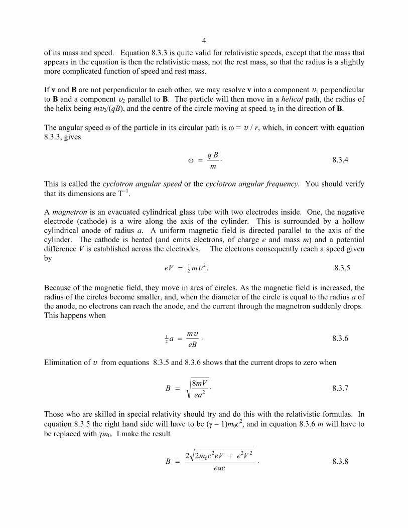
4of its mass and speed. Equation 8.3.3 is quite valid for relativistic speeds, except that the mass that appears in the equation is then the relativistic mass, not the rest mass, so that the radius is a slightly more complicated function of speed and rest mass. If v and B are not perpendicular to each other, we may resolve v into a component v1 perpendicular to B and a component v2 parallel to B. The particle will then move in a helical path, the radius of the helix being mv2/(qB), and the centre of the circle moving at speed v2 in the direction of B. The angular speed ω of the particle in its circular path is ω = v / r, which, in concert with equation 8.3.3, gives

ω =q Bm

. 8.3.4

This is called the cyclotron angular speed or the cyclotron angular frequency. You should verify that its dimensions are T−1. A magnetron is an evacuated cylindrical glass tube with two electrodes inside. One, the negative electrode (cathode) is a wire along the axis of the cylinder. This is surrounded by a hollow cylindrical anode of radius a. A uniform magnetic field is directed parallel to the axis of the cylinder. The cathode is heated (and emits electrons, of charge e and mass m) and a potential difference V is established across the electrodes. The electrons consequently reach a speed given by eV m= 1

22v . 8.3.5

Because of the magnetic field, they move in arcs of circles. As the magnetic field is increased, the radius of the circles become smaller, and, when the diameter of the circle is equal to the radius a of the anode, no electrons can reach the anode, and the current through the magnetron suddenly drops. This happens when

12 a m

eB=

v . 8.3.6

Elimination of v from equations 8.3.5 and 8.3.6 shows that the current drops to zero when

.82ea

mVB = 8.3.7

Those who are skilled in special relativity should try and do this with the relativistic formulas. In equation 8.3.5 the right hand side will have to be (γ − 1)m0c2, and in equation 8.3.6 m will have to be replaced with γm0. I make the result

.22 2220

eacVeeVcm

B+

= 8.3.8

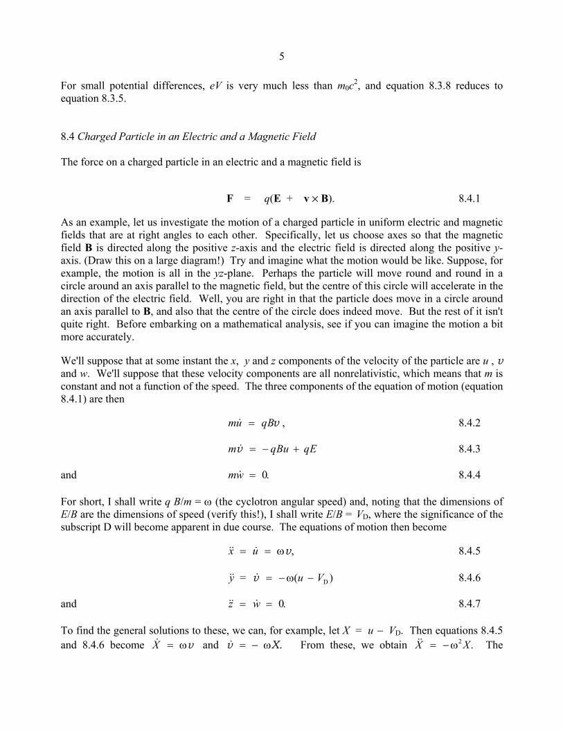
5 For small potential differences, eV is very much less than m0c2, and equation 8.3.8 reduces to equation 8.3.5. 8.4 Charged Particle in an Electric and a Magnetic Field The force on a charged particle in an electric and a magnetic field is

F = q(E + v % B). 8.4.1

As an example, let us investigate the motion of a charged particle in uniform electric and magnetic fields that are at right angles to each other. Specifically, let us choose axes so that the magnetic field B is directed along the positive z-axis and the electric field is directed along the positive y-axis. (Draw this on a large diagram!) Try and imagine what the motion would be like. Suppose, for example, the motion is all in the yz-plane. Perhaps the particle will move round and round in a circle around an axis parallel to the magnetic field, but the centre of this circle will accelerate in the direction of the electric field. Well, you are right in that the particle does move in a circle around an axis parallel to B, and also that the centre of the circle does indeed move. But the rest of it isn't quite right. Before embarking on a mathematical analysis, see if you can imagine the motion a bit more accurately.

We'll suppose that at some instant the x, y and z components of the velocity of the particle are u , v and w. We'll suppose that these velocity components are all nonrelativistic, which means that m is constant and not a function of the speed. The three components of the equation of motion (equation 8.4.1) are then

, vBqum =& 8.4.2

EqBuqm +−=v& 8.4.3

and .0=wm & 8.4.4

For short, I shall write q B/m = ω (the cyclotron angular speed) and, noting that the dimensions of E/B are the dimensions of speed (verify this!), I shall write E/B = VD, where the significance of the subscript D will become apparent in due course. The equations of motion then become

,vω== ux &&& 8.4.5

)( DVu=y −ω−=v&&& 8.4.6

and .0== wz &&& 8.4.7

To find the general solutions to these, we can, for example, let X = u − VD. Then equations 8.4.5 and 8.4.6 become X.vv ω−=ω= && andX From these, we obtain .2 XX ω−=&& The

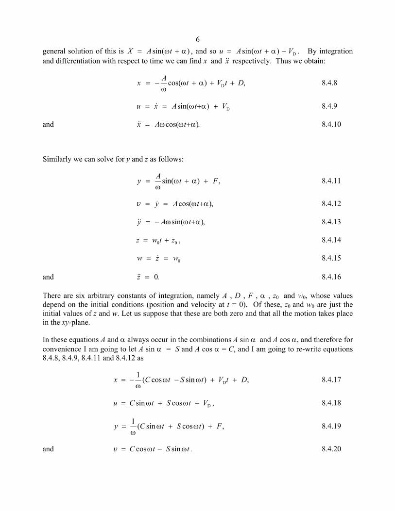
6general solution of this is X A t= +sin( ) ,ω α and so u A t= + +sin( ) .ω α VD By integration and differentiation with respect to time we can find x and x&& respectively. Thus we obtain:

,)cos( D DtVtAx ++α+ωω

−= 8.4.8

D)sin( VtAxu +α+ω== & 8.4.9

and .)cos( α+ωω= tAx&& 8.4.10

Similarly we can solve for y and z as follows:

,)sin( FtAy +α+ωω

= 8.4.11

,)cos( α+ω== tAy&v 8.4.12

,)sin( α+ωω−= tAy&& 8.4.13

z w t z= +0 0 , 8.4.14

0wzw == & 8.4.15

and .0=z&& 8.4.16

There are six arbitrary constants of integration, namely A , D , F , α , z0 and w0, whose values depend on the initial conditions (position and velocity at t = 0). Of these, z0 and w0 are just the initial values of z and w. Let us suppose that these are both zero and that all the motion takes place in the xy-plane.

In these equations A and α always occur in the combinations A sin α and A cos α, and therefore for convenience I am going to let A sin α = S and A cos α = C, and I am going to re-write equations 8.4.8, 8.4.9, 8.4.11 and 8.4.12 as

,)sincos(1D DtVtStCx ++ω−ω

ω−= 8.4.17

,cossin DVtStCu +ω+ω= 8.4.18

,)cossin(1 FtStCy +ω+ωω

= 8.4.19

and .sincos tStC ω−ω=v 8.4.20

7Let is suppose that the initial conditions are: at t = 0, x = y = u = v = 0. That is, the particle starts from rest at the origin. If the put these initial conditions in equations 8.4.17-20, we find that C = 0, S = −VD, D = 0 and F = VD/ω. Equations 8.4.17 and 8.4.19, which give the equation to the path described by the particle, become

tVtVx DD sin +ω

ω−= 8.4.21

and .)cos1(D tVy ω−ω

= 8.4.22

It is worth reminding ourselves here that the cyclotron angular speed is ω = qB/m and that VD =

E/B, and therefore .2

D

qBmEV

=ω

These equations are the parametric equations of a cycloid. (For

more on the cycloid, see Chapter 19 of the Classical Mechanics notes in this series.) The motion is a circular motion in which the centre of the circle drifts (hence the subscript D) in the x-direction at

speed VD. The path is shown in figure VIII.2, drawn for distances in units of 2D

qBmEV

=ω

.

0 2 4 6 8 10 120

1

2

3

x

y

FIGURE VIII.2

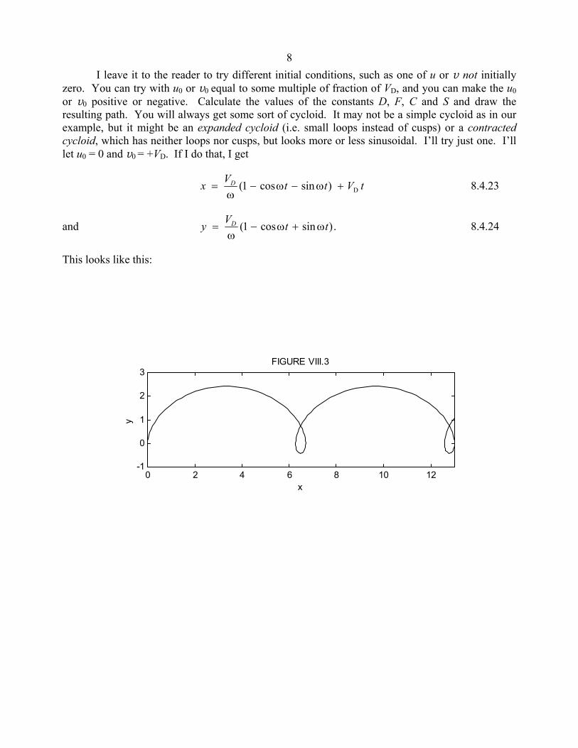
8 I leave it to the reader to try different initial conditions, such as one of u or v not initially zero. You can try with u0 or v0 equal to some multiple of fraction of VD, and you can make the u0 or v0 positive or negative. Calculate the values of the constants D, F, C and S and draw the resulting path. You will always get some sort of cycloid. It may not be a simple cycloid as in our example, but it might be an expanded cycloid (i.e. small loops instead of cusps) or a contracted cycloid, which has neither loops nor cusps, but looks more or less sinusoidal. I’ll try just one. I’ll let u0 = 0 and v0 = +VD. If I do that, I get

tVttVx DD)sincos1( +ω−ω−

ω= 8.4.23

and .)sincos1( ttVy D ω+ω−ω

= 8.4.24

This looks like this:

0 2 4 6 8 10 12-1

0

1

2

3

x

y

FIGURE VIII.3

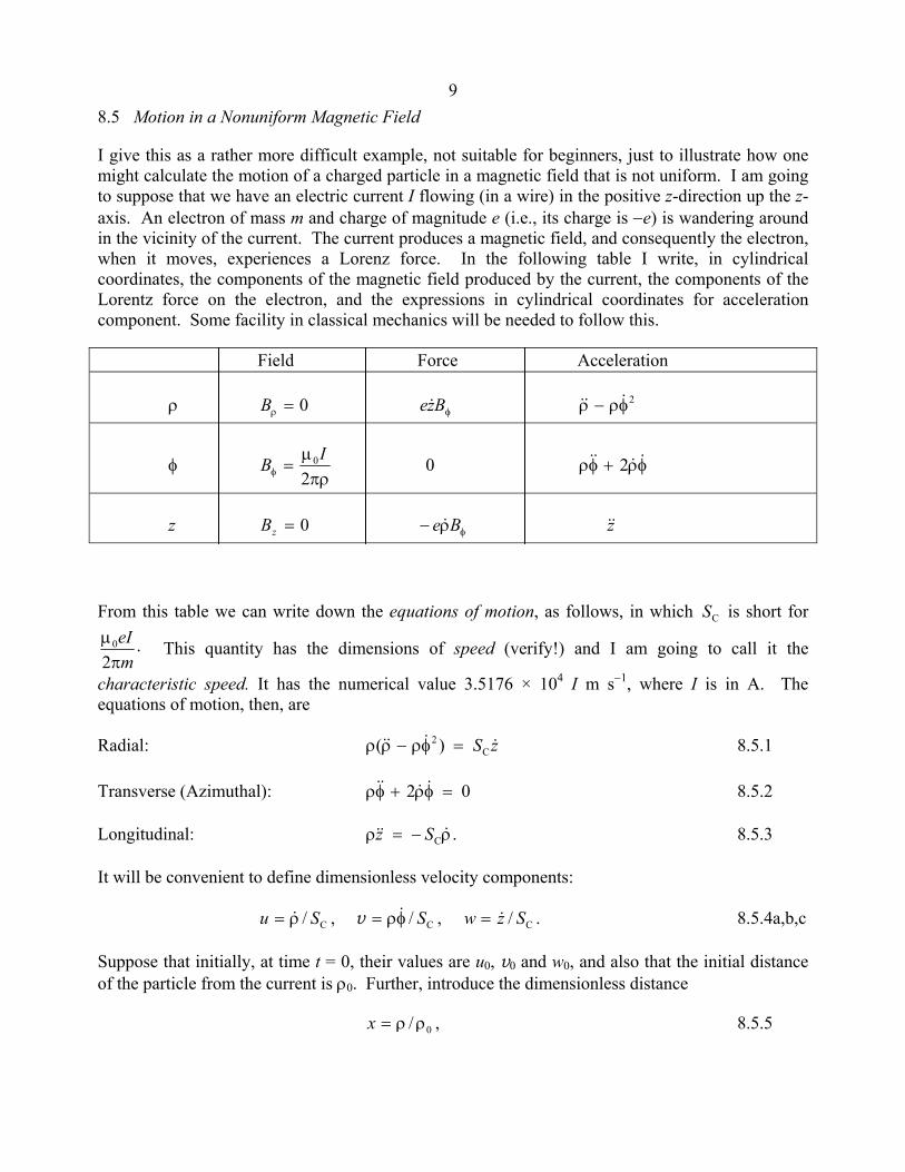
98.5 Motion in a Nonuniform Magnetic Field

I give this as a rather more difficult example, not suitable for beginners, just to illustrate how one might calculate the motion of a charged particle in a magnetic field that is not uniform. I am going to suppose that we have an electric current I flowing (in a wire) in the positive z-direction up the z-axis. An electron of mass m and charge of magnitude e (i.e., its charge is −e) is wandering around in the vicinity of the current. The current produces a magnetic field, and consequently the electron, when it moves, experiences a Lorenz force. In the following table I write, in cylindrical coordinates, the components of the magnetic field produced by the current, the components of the Lorentz force on the electron, and the expressions in cylindrical coordinates for acceleration component. Some facility in classical mechanics will be needed to follow this.

Field Force Acceleration

ρ 0=ρB φBze& 2φρ−ρ &&&

φ πρ

µ=φ 2

0IB 0 φρ+φρ &&&& 2

z 0=zB φρ− Be & z&&

From this table we can write down the equations of motion, as follows, in which CS is short for

.2

0

meI

πµ This quantity has the dimensions of speed (verify!) and I am going to call it the

characteristic speed. It has the numerical value 3.5176 × 104 I m s−1, where I is in A. The equations of motion, then, are

Radial: zS &&&& C2 )( =φρ−ρρ 8.5.1

Transverse (Azimuthal): 02 =φρ+φρ &&&& 8.5.2

Longitudinal: .Cρ−=ρ &&& Sz 8.5.3

It will be convenient to define dimensionless velocity components:

./,/,/ CCC SzwSSu &&& =φρ=ρ= v 8.5.4a,b,c

Suppose that initially, at time t = 0, their values are u0, v0 and w0, and also that the initial distance of the particle from the current is ρ0. Further, introduce the dimensionless distance

,/ 0ρρ=x 8.5.5

10so that the initial value of x is 1. The initial values of φ and z may be taken to be zero by suitable choice of axes.

Integration of equations 8.5.2 and 3, with these initial conditions, yields

( ))/ln( 00 ρρ−= wSz C& 8.5.6

and ;C002 Svρ=φρ & 8.5.7

or, in terms of the dimensionless variables,

xww ln0 −= 8.5.8

and ./0 xvv = 8.5.9

We may write ρρρ

ρ &&&

& fordd in equation 8.5.1, and substitution for z& and φ& from equations 8.5.6 and

8.5.7 yields

.)(lnln2)/11( 20

220

20

2 xxwxuu −+−+= v 8.5.10

Equations 8.5.8,9 and 10 give the velocity components of the electron as a function of its distance from the wire.

Equation 8.5.2 expresses the fact that there is no transverse (azimuthal) force. Its time integral, equation 8.5.7) expresses the consequence that the z-component of its angular momentum is conserved. Further, from equations 8.5.8,9 and 10, we find that

,say,220

20

20

222 swuwu =++=++ vv 8.5.11

so that the speed of the electron is constant. This is as expected, since the force on the electron is always perpendicular to its velocity; the point of applicat6ion of the force does not move in the direction of the force, which therefore does no work, so that kinetic energy, and hence speed, is conserved.

The distance of the electron from the wire is bounded below and above. The lower and upper bounds, x1 and x2 are found from equation 8.5.10 by putting u = 0 and solving for x. Examples of these bounds are shown in the Table VIII.I for a variety of initial conditions.

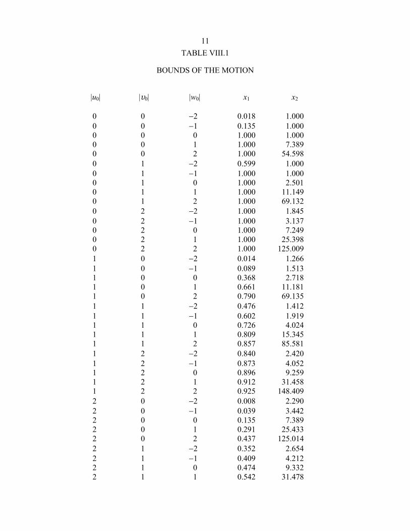
11TABLE VIII.1

BOUNDS OF THE MOTION

|u0| |v0| |w0| x1 x2 0 0 −2 0.018 1.000 0 0 −1 0.135 1.000 0 0 0 1.000 1.000 0 0 1 1.000 7.389 0 0 2 1.000 54.598 0 1 −2 0.599 1.000 0 1 −1 1.000 1.000 0 1 0 1.000 2.501 0 1 1 1.000 11.149 0 1 2 1.000 69.132 0 2 −2 1.000 1.845 0 2 −1 1.000 3.137 0 2 0 1.000 7.249 0 2 1 1.000 25.398 0 2 2 1.000 125.009 1 0 −2 0.014 1.266 1 0 −1 0.089 1.513 1 0 0 0.368 2.718 1 0 1 0.661 11.181 1 0 2 0.790 69.135 1 1 −2 0.476 1.412 1 1 −1 0.602 1.919 1 1 0 0.726 4.024 1 1 1 0.809 15.345 1 1 2 0.857 85.581 1 2 −2 0.840 2.420 1 2 −1 0.873 4.052 1 2 0 0.896 9.259 1 2 1 0.912 31.458 1 2 2 0.925 148.409 2 0 −2 0.008 2.290 2 0 −1 0.039 3.442 2 0 0 0.135 7.389 2 0 1 0.291 25.433 2 0 2 0.437 125.014 2 1 −2 0.352 2.654 2 1 −1 0.409 4.212 2 1 0 0.474 9.332 2 1 1 0.542 31.478

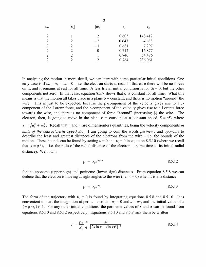
12 |u0| |v0| |w0| x1 x2 2 1 2 0.605 148.412 2 2 −2 0.647 4.183 2 2 −1 0.681 7.297 2 2 0 0.712 16.877 2 2 1 0.740 54.486 2 2 2 0.764 236.061 In analysing the motion in more detail, we can start with some particular initial conditions. One easy case is if u0 = v0 = w0 = 0 – i.e. the electron starts at rest. In that case there will be no forces on it, and it remains at rest for all time. A less trivial initial condition is for v0 = 0, but the other components not zero. In that case, equation 8.5.7 shows that φ is constant for all time. What this means is that the motion all takes place in a plane φ = constant, and there is no motion “around” the wire. This is just to be expected, because the ρ-component of the velocity gives rise to a z-component of the Lorenz force, and the z-component of the velocity gives rise to a Lorentz force towards the wire, and there is no component of force “around” (increasing φ) the wire. The electron, then, is going to move in the plane φ = constant at a constant speed ,CsSS = where

.20

20 wus += (Recall that u and w are dimensionless quantities, being the velocity components in

units of the characteristic speed SC.) I am going to coin the words perineme and aponeme to describe the least and greatest distances of the electrons from the wire – i.e. the bounds of the motion. These bounds can be found by setting u = 0 and v0 = 0 in equation 8.5.10 (where we recall that 0/ρρ=x - i.e. the ratio of the radial distance of the electron at some time to its initial radial distance). We obtain swe ±ρ=ρ 0

0 8.5.12 for the aponeme (upper sign) and perineme (lower sign) distances. From equation 8.5.8 we can deduce that the electron is moving at right angles to the wire (i.e. w = 0) when it is at a distance .0

0weρ=ρ 8.5.13

The form of the trajectory with v0 = 0 is found by integrating equations 8.5.8 and 8.5.10. It is convenient to start the integration at perineme so that u0 = 0 and s = w0, and the initial value of x

)/( 0ρρ= is 1. For any other initial conditions, the perineme values of x and ρ can be found from equations 8.5.10 and 8.5.12 respectively. Equations 8.5.10 and 8.5.8 may them be written

2/12C

0

])(lnln2[1 xxsdx

St

x

−ρ

= ∫ 8.5.14

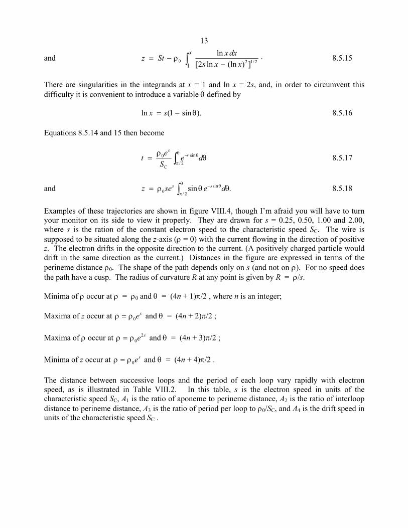
13

and .])(lnln2[

ln2/120

1 xxsdxxStz

x

−ρ−= ∫ 8.5.15

There are singularities in the integrands at x = 1 and ln x = 2s, and, in order to circumvent this difficulty it is convenient to introduce a variable θ defined by ).sin1(ln θ−= sx 8.5.16 Equations 8.5.14 and 15 then become

θρ

= ∫θ

π

θ− deS

et ss

2/

sin

C

0 8.5.17

and .sin2/

sin0 θθρ= ∫

θ

π

θ− desez ss 8.5.18

Examples of these trajectories are shown in figure VIII.4, though I’m afraid you will have to turn your monitor on its side to view it properly. They are drawn for s = 0.25, 0.50, 1.00 and 2.00, where s is the ration of the constant electron speed to the characteristic speed SC. The wire is supposed to be situated along the z-axis (ρ = 0) with the current flowing in the direction of positive z. The electron drifts in the opposite direction to the current. (A positively charged particle would drift in the same direction as the current.) Distances in the figure are expressed in terms of the perineme distance ρ0. The shape of the path depends only on s (and not on ρ). For no speed does the path have a cusp. The radius of curvature R at any point is given by R = ρ/s. Minima of ρ occur at ρ = ρ0 and θ = (4n + 1)π/2 , where n is an integer; Maxima of z occur at se0ρ=ρ and θ = (4n + 2)π/2 ; Maxima of ρ occur at se2

0ρ=ρ and θ = (4n + 3)π/2 ; Minima of z occur at se0ρ=ρ and θ = (4n + 4)π/2 . The distance between successive loops and the period of each loop vary rapidly with electron speed, as is illustrated in Table VIII.2. In this table, s is the electron speed in units of the characteristic speed SC, A1 is the ratio of aponeme to perineme distance, A2 is the ratio of interloop distance to perineme distance, A3 is the ratio of period per loop to ρ0/SC, and A4 is the drift speed in units of the characteristic speed SC .

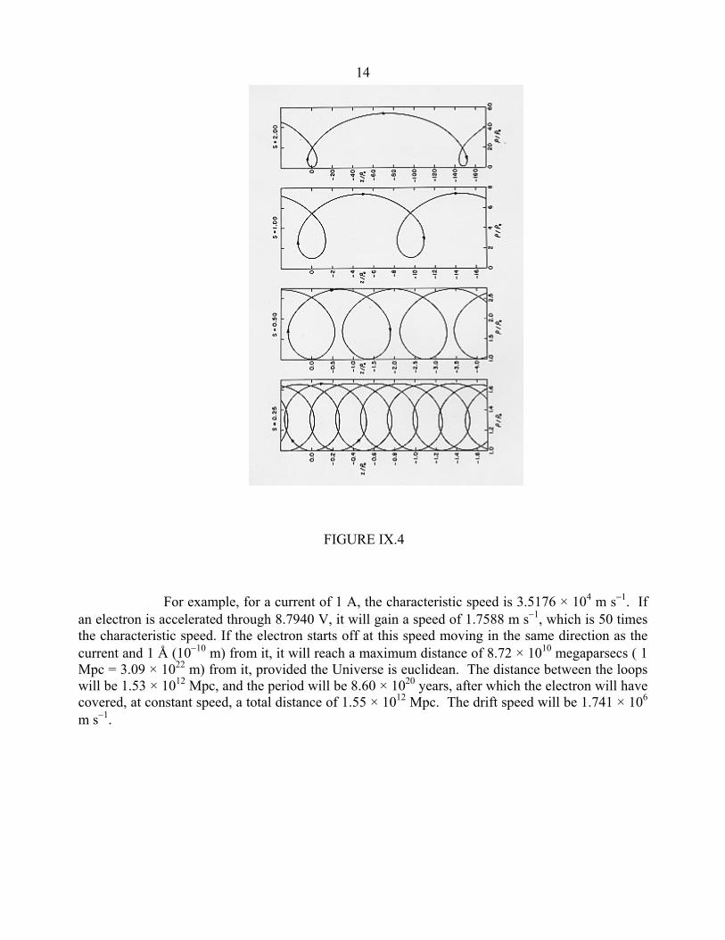
14

FIGURE IX.4

For example, for a current of 1 A, the characteristic speed is 3.5176 × 104 m s−1. If an electron is accelerated through 8.7940 V, it will gain a speed of 1.7588 m s−1, which is 50 times the characteristic speed. If the electron starts off at this speed moving in the same direction as the current and 1 Å (10−10 m) from it, it will reach a maximum distance of 8.72 × 1010 megaparsecs ( 1 Mpc = 3.09 × 1022 m) from it, provided the Universe is euclidean. The distance between the loops will be 1.53 × 1012 Mpc, and the period will be 8.60 × 1020 years, after which the electron will have covered, at constant speed, a total distance of 1.55 × 1012 Mpc. The drift speed will be 1.741 × 106

m s−1.

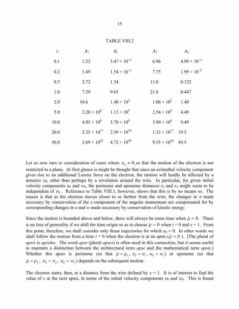
15

TABLE VIII.2

s A1 A2 A3 A4

0.1 1.22 3.47 × 10−2 6.96 4.99 × 10−3

0.2 1.49 1.54 × 10−1 7.75 1.99 × 10−2

0.5 2.72 1.34 11.0 0.122

1.0 7.39 9.65 21.6 0.447

2.0 54.6 1.48 × 102 1.06 × 102 1.40

5.0 2.20 × 104 1.13 × 105 2.54 × 104 4.49

10.0 4.85 × 108 3.70 × 109 3.90 × 108 9.49

20.0 2.35 × 1017 2.59 × 1018 1.33 × 1017 19.5

50.0 2.69 × 1043 4.73 × 1044 9.55 × 1042 49.5

Let us now turn to consideration of cases where ,00 ≠v so that the motion of the electron is not restricted to a plane. At first glance is might be thought that since an azimuthal velocity component gives rise to no additional Lorenz force on the electron, the motion will hardly be affected by a nonzero v0, other than perhaps by a revolution around the wire. In particular, for given initial velocity components u0 and w0, the perineme and aponeme distances x1 and x2 might seem to be independent of v0 . Reference to Table VIII.1, however, shows that this is by no means so. The reason is that as the electron moves closer to or further from the wire, the changes in v made necessary by conservation of the z-component of the angular momentum are compensated for by corresponding changes in u and w made necessary by conservation of kinetic energy. Since the motion is bounded above and below, there will always be some time when .0=ρ& There is no loss of generality if we shift the time origin so as to choose 0=ρ& when t = 0 and x = 1. From this point, therefore, we shall consider only those trajectories for which u0 = 0. In other words we shall follow the motion from a time t = 0 when the electron is at an apsis ( 0=ρ& ). [The plural of apsis is apsides. The word apse (plural apses) is often used in this connection, but it seems useful to maintain a distinction between the architectural term apse and the mathematical term apsis.] Whether this apsis is perineme (so that 10101 ,, ww ==ρ=ρ vv& ) or aponeme (so that

20202 ,, ww ==ρ=ρ vv& ) depends on the subsequent motion. The electron starts, then, at a distance from the wire defined by x = 1. It is of interest to find the value of x at the next apsis, in terms of the initial velocity components v0 and w0. This is found

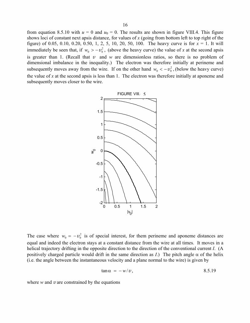
16from equation 8.5.10 with u = 0 and u0 = 0. The results are shown in figure VIII.4. This figure shows loci of constant next apsis distance, for values of x (going from bottom left to top right of the figure) of 0.05, 0.10, 0.20, 0.50, 1, 2, 5, 10, 20, 50, 100. The heavy curve is for x = 1. It will immediately be seen that, if ,2

00 v−>w (above the heavy curve) the value of x at the second apsis is greater than 1. (Recall that v and w are dimensionless ratios, so there is no problem of dimensional imbalance in the inequality.) The electron was therefore initially at perineme and subsequently moves away from the wire. If on the other hand ,2

00 v−<w (below the heavy curve) the value of x at the second apsis is less than 1. The electron was therefore initially at aponeme and subsequently moves closer to the wire.

0 0.5 1 1.5 2-2

-1.5

-1

-0.5

0

0.5

1

1.5

2

|v0|

w0

FIGURE VIII.4

The case where 200 v−=w is of special interest, for them perineme and aponeme distances are

equal and indeed the electron stays at a constant distance from the wire at all times. It moves in a helical trajectory drifting in the opposite direction to the direction of the conventional current I. (A positively charged particle would drift in the same direction as I.) The pitch angle α of the helix (i.e. the angle between the instantaneous velocity and a plane normal to the wire) is given by

,/tan vw−=α 8.5.19

where w and v are constrained by the equations

5

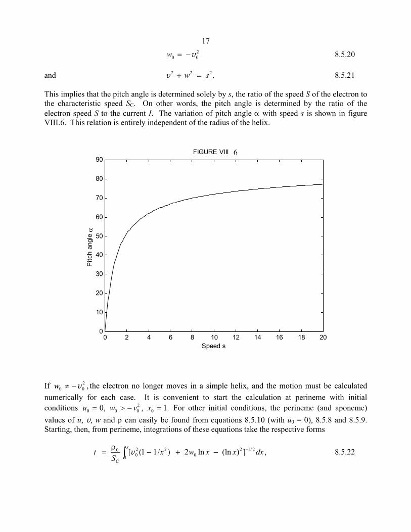
17

200 v−=w 8.5.20

and .222 sw =+v 8.5.21

This implies that the pitch angle is determined solely by s, the ratio of the speed S of the electron to the characteristic speed SC. On other words, the pitch angle is determined by the ratio of the electron speed S to the current I. The variation of pitch angle α with speed s is shown in figure VIII.6. This relation is entirely independent of the radius of the helix.

0 2 4 6 8 10 12 14 16 18 200

10

20

30

40

50

60

70

80

90

Pitc

h an

gle

α

Speed s

FIGURE VIII.5

If ,200 v−≠w the electron no longer moves in a simple helix, and the motion must be calculated

numerically for each case. It is convenient to start the calculation at perineme with initial conditions .1,,0 0

2000 =−>= xvwu For other initial conditions, the perineme (and aponeme)

values of u, v, w and ρ can easily be found from equations 8.5.10 (with u0 = 0), 8.5.8 and 8.5.9. Starting, then, from perineme, integrations of these equations take the respective forms

∫ −−+−ρ

=x

dxxxwxS

t1

2/120

220

C

0 ,])(lnln2)/11([v 8.5.22

6

18

∫ −−+−ρ−=x

dxxxxwxtSwz1

2/120

2200C0 ln])(lnln2)/11([v 8.5.23

and ∫ −−−+−=φx

dxxxxwx1

22/120

2200 .])(lnln2)/11([vv 8.5.24

The integration of these equations is not quite trivial and is discussed in the Appendix (Section 8A).

In general the motion of the electron can be described qualitatively roughly as follows. The motion is bounded between two cylinders of radii equal to the perineme and aponeme distances, and the speed is constant. The electron moves around the wire in either a clockwise or a counterclockwise direction, but, once started, the sense of this motion does not change. The angular speed around the wire is greatest at perineme and least at aponeme, being inversely proportional to the square of the distance from the wire. Superimposed on the motion around the wire is a general drift in the opposite direction to that of the conventional current. However, for a brief moment near perineme the electron is temporarily moving in the same direction as the current.

An example of the motion is given in figures VIII.7 and 8 for initial velocity components u0 = 0, v0 = w0 = 1. The aponeme distance is 11.15 times the perineme distance. The time interval between two perineme passages is 26.47 ρ0/SC . The time interval for a complete revolution around the wire (φ = 360o) is 68.05 ρ0/SC . In figure VIII.8, the conventional electric current is supposed to be flowing into the plane of the “paper” (computer screen), away from the reader. The portions of the electron trajectory where the electron is moving towards from the reader are drawn as a continuous line, and the brief portions near perineme where the electron is moving away from the reader are indicated by a dotted line. Time marks on the figure are at intervals of 5ρ0/SC .

19

FIGURE VIII.7

FIGURE VIII.8

208A Appendix. Integration of the Equations

Numerical integration of equations 8.5.22-24 is straightforward (by Simpson’s rule, for example) except near perineme (x = 1) and aponeme (x = x2), where the integrands become infinite. Near perineme, however, we can substitute

ξ+= 1x and near aponeme we can substitute ),ξ−= 1(2xx and we can expand the integrands as power series in ξ and integrate term by term. I gather here the following results for the intervals x = 1 to x = 1 + ε and x = x2 − ε to x = x2, where ε must be chosen to be sufficiently small that ε4 is smaller than the precision required.

)1(])(lnln2)/11([ 317

121

1

1 51

1312/12

022

01 K+ε+ε+ε+=−+−= ∫ε+ − CBAMdxxxwxI v 8A.1

)(ln])(lnln2)/11([ 317

121

1

1 51

312/12

022

02 K+ε+ε+ε=−+−= ∫ε+ − EDMxdxxxwxI v 8A.2

)1(])(lnln2)/11([ 317

121

1

1 51

13122/12

022

03 K+ε+ε+ε+=−+−= ∫ε+ −− HGFMdxxxxwxI v 8A.3

))/()/(/1[])(lnln2)/11([ 3227

12225

1223

12/120

2204

2

2

K+ε+ε+ε+=−+−= ∫ ε−

− xCxBxANdxxxwxIx

xv

8A.4

∫ ε−

−−+−= 2

2

ln])(lnln2)/11([ 2/120

2205

x

xxdxxxwxI v

])/()/(/[ln 3227

12225

123

124 K+ε+ε+ε−= xExDxNxI 8A.5

∫ ε−

−−−+−= 2

2

22/120

2206 ])(lnln2)/11([

x

xdxxxxwxI v

22

3227

12225

1223

1 /])/()/(/1[ xxHxGxFN K+ε+ε+ε+= 8A.6

The constants are defined as follows.

2/1

020

2

+ε

=w

Mv

8A.7

2/1

02

202

2

)/(ln2

−−

ε=

wxxxN

v 8A.8

)(213

020

020

1 wwa+

++−=

vv

8A.9

)(2

14

020

0322

01 w

wb+

++=

vv

8A.10

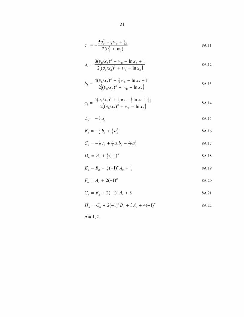
21

)(2

5

020

1211

0212

01 w

wc+

++−=

vv

8A.11

( )202

20

202

202 ln)/(2

1ln)/(3xwx

xwxa−+

+−+=

vv

8A.12

( )202

20

20322

202 ln)/(2

1ln)/(4xwx

xwxb−+

+−+=

vv

8A.13

( )202

20

1211

221

0212

202 ln)/(2

ln)/(5xwx

xwxc−+

+−+=

vv

8A.14

nn aA 21−= 8A.15

283

21

nnn abB +−= 8A.16

3165

43

21

nnnnn abacC −+−= 8A.17

nnn AD )1(2

1 −+= 8A.18

31

21 )1( +−+= n

nnn ABE 8A.19

nnn AF )1(2 −+= 8A.20

3)1(2 +−+= nn

nn ABG 8A.21

nnn

nnn ABCH )1(43)1(2 −++−+= 8A.22

2,1=n

1

CHAPTER 9 MAGNETIC POTENTIAL

9.1 Introduction We are familiar with the idea that an electric field E can be expressed as minus the gradient of a potential function V. That is E = −grad V = −=V. 9.1.1 Note that V is not unique, because an arbitrary constant can be added to it. We can define a unique V by assigning a particular value of V to some point (such as zero at infinity). Can we express the magnetic field B in a similar manner as the gradient of some potential function ψ, so that, for example, B = −grad ψ = −=ψ ? Before answering this, we note that there are some differences between E and B . Unlike E, the magnetic field B is sourceless; there are no sources or sinks; the magnetic field lines are closed loops. The force on a charge q in an electric field is qE, and it depends only on where the charge is in the electric field – i.e. on its position. Thus the force is conservative, and we understand from any study of classical mechanics that only conservative forces can be expressed as the derivative of a potential function. The force on a charge q in a magnetic field is qv % B. This force (the Lorentz force) does not depend only on the position of the particle, but also on its velocity (speed and direction). Thus the force is not conservative. This suggests that perhaps we cannot express the magnetic field merely as the gradient of a scalar potential function – and this is correct; we cannot. 9.2 The Magnetic Vector Potential Although we cannot express the magnetic field as the gradient of a scalar potential function, we shall define a vector quantity A whose curl is equal to the magnetic field: B = curl A = = % A . 9.2.1 Just as E = −=V does not define V uniquely (because we can add an arbitrary constant to it, so, similarly, equation 9.2.1 does not define A uniquely. For, if ψ is some scalar quantity, we can always add =ψ to A without affecting B, because = % =ψ = curl grad ψ = 0. The vector A is called the magnetic vector potential. Its dimensions are MLT−1Q−1. Its SI units can be expressed as T m, or Wb m−1 or N A−1. It might be briefly noted here that some authors define the magnetic vector potential from H = curl A, though it is standard SI practice to define it from B = curl A. Systems of units and definitions other than SI will be dealt with in Chapter 16.

2

Now in electrostatics, we have rE ˆ41

2rq

πε= for the electric field near a point charge, and, with E

= −grad V, we obtain for the potential .4 r

qVπε

= In electromagnetism we have

dsrdB ×ˆ4 2r

Iπµ

= for the contribution to the magnetic field near a circuit element ds. Given that B

= curl A, can we obtain an expression for the magnetic vector potential from the current element? The answer is yes, if we recognize that 2/ˆ rr can be written −∇( / ) .1 r (If this isn't obvious, go to the expression for ∇ψ in spherical coordinates, and put ψ = 1/r.) The Biot-Savart law becomes

dB ds ds= − =µ

πµ

πI r I r

41

41∇ × × ∇( / ) ( / ) . 9.2.3

Since ds is independent of r, the nabla can be moved to the left of the cross product to give

.4

dsdBr

Iπµ

= ×∇ 9.2.4

The expression µπIr4

ds, then, is the contribution dA to the magnetic vector potential from the

circuit element ds. Of course an isolated circuit element cannot exist by itself, so, for the magnetic vector potential from a complete circuit, the line integral of this must be calculated around the circuit. 9.3 Long, Straight, Current-carrying Conductor

By way of example, let us use the expression dA ds=µπIr4

, to calculate the magnetic vector

potential in the vicinity of a long, straight, current-carrying conductor ("wire" for short!). We'll suppose that the wire lies along the z-axis, with the current flowing in the direction of positive z. We'll work in cylindrical coordinates, and the symbols z,ˆ,ˆ φρ will denote the unit orthogonal vectors. After we have calculated A, we'll try and calculate its curl to give us the magnetic field B.

We already know, of course, that for a straight wire the field is φ2πρµ

=IB , so this will serve as a

check on our algebra. Consider an element dzz on the wire at a height z above the xy-plane. (The length of this element is dz; the unit vector z just indicates its direction.) Consider also a point P in the xy-plane at a distance ρ from the wire. The distance of P from the element dz is ρ2 2+ z . The contribution to the magnetic vector potential is therefore

3

.)(

.4

ˆ 2/122 zdzI

+ρπµ

= zdA 9.3.1

The total magnetic vector potential is therefore

.)(

.2

ˆ0 2/122∫∞

+ρπµ

=z

dzIzA 9.3.2

This integral is infinite, which at first may appear to be puzzling. Let us therefore first calculate the magnetic vector potential for a finite section of length 2l of the wire. For this section, we have

.)(

.2

ˆ0 2/122∫ +ρπ

µ=

l

zdzIzA 9.3.3

To integrate this, let z = ρ tan θ, whence ,sec.2

ˆ0∫α

θθπ

µ= dIzA where l = ρ tan α. From this we

obtain ,)tanln(sec.2

ˆ α+απ

µ=

IzA whence

.ln.2

ˆ22

ρ+ρ+

πµ

=llIzA 9.3.4

For l >> ρ this becomes ).ln2(ln2

ˆ2ln.2

ˆ ρ−π

µ=

ρπ

µ= lIlI zzA 9.3.5

Thus we see that the magnetic vector potential in the vicinity of a straight wire is a vector field parallel to the wire. If the wire is of infinite length, the magnetic vector potential is infinite. For a finite length, the potential is given exactly by equation 9.3.4, and, very close to a long wire, the potential is given approximately by equation 9.3.5. Now let us use equation 9.3.5 together with B = curl A, to see if we can find the magnetic field B. We'll have to use the expression for curl A in cylindrical coordinates, which is

.ˆ1ˆˆ1 zAcurl

∂φ∂

−∂ρ∂

ρ+ρ

+

∂ρ∂

−∂

∂+

∂

∂−

∂φ∂

ρ= ρφ

φρφ AA

AAz

Az

AA zz φρ 9.3.6

In our case, A has only a z-component, so this is much simplified:

.ˆˆ1φρ

∂ρ∂

−∂φ∂

ρ= zz AAAcurl 9.3.7

4

And since the z-component of A depends only on ρ, the calculation becomes trivial, and we obtain, as expected

.ˆ2

φπρ

µ=

IB 9.3.8

This is an approximate result for very close to a long wire – but it is exact for any distance for an infinite wire. This may strike you as a long palaver to derive equation 9.3.8 – but the object of the exercise was not to derive equation 9.3.8 (which is trivial from Ampère's theorem), but to derive the expression for A. Calculating B subsequently was only to reassure us that our algebra was correct. 9.4 Long Solenoid Let us place an infinitely long solenoid of n turns per unit length so that its axis coincides with the z-axis of coordinates, and the current I flows in the sense of increasing φ. In that case, we already know that the field inside the solenoid is uniform and is zInµ inside the solenoid and zero outside. Since the field has only a z component, the vector potential A cam have only a φ-component. We'll suppose that the radius of the solenoid is a. Now consider a circle of radius r (less than a) perpendicular to the axis of the solenoid (and hence to the field B). The magnetic flux through this circle (i.e. the surface integral of B across the circle) is π r B2 = π r2nI. Now, as everybody knows, the surface integral of a vector field across a closed curve is equal to the line integral of its curl around the curve, and this is equal to 2π r Aφ. Thus, inside the solenoid the vector potential is .ˆ

21 φIrnµ=A 9.4.1

It is left to the reader to argue that, outside the solenoid (r > a), the magnetic vector potential is

.ˆ2

2

φr

Ianµ=A 9.4.2

9.5 Divergence Like the magnetic field itself, the lines of magnetic vector potential form closed loops (except in the case of the infinitely long straight conducting wire, in which case they are infinitely long straight lines). That is to say A has no sources or sinks, or, in other words, its divergence is everywhere zero: div A = 0. 9.5.1

1

CHAPTER 10 ELECTROMAGNETIC INDUCTION

10.1 Introduction In 1820, Oersted had shown that an electric current generates a magnetic field. But can a magnetic field generate an electric current? This was answered almost simultaneously and independently in 1831 by Joseph Henry in the United States and Michael Faraday in Great Britain. Faraday constructed an iron ring, about six inches in diameter. He wound two coils of wire tightly around the ring; one coil around one half (semicircle) of the ring, and the second coil around the second half of the ring. The two coils were not connected to one another other than by sharing the same iron core. One coil (which I'll refer to as the "primary" coil") was connected to a battery; the other coil (which I'll refer to as the "secondary" coil) was connected to a galvanometer. When the battery was connected to the primary coil a current, of course, flowed through the primary coil. This current generated a magnetic field throughout the iron core, so that there was a magnetic field inside each of the two coils. As long as the current in the primary coil remained constant, there was no current in the secondary coil. What Faraday observed was that at the instant when the battery was connected to the primary, and during that brief moment when the current in the primary was rising from zero, a current momentarily flowed in the secondary – but only while the current in the primary was changing. When the battery was disconnected, and during the brief moment when the primary current was falling to zero, again a current flowed in the secondary (but in the opposite direction to previously). Of course, while the primary current was changing, the magnetic field in the iron core was changing, and Faraday recognized that a current was generated in the secondary while the magnetic flux through it was changing. The strength of the current depended on the resistance of the secondary, so it is perhaps more fundamental to note that when the magnetic flux through a circuit changes, an electromotive force (EMF) is generated in the circuit, and the faster the flux changes, the greater the induced EMF. Quantitative measurements have long established that: While the magnetic flux through a circuit is changing, an EMF is generated in the circuit which is equal to the rate of change of magnetic flux BΦ& through the circuit. This is generally called "Faraday's Law of Electromagnetic Induction". A complete statement of the laws of electromagnetic induction must also tell us the direction of the induced EMF, and this is generally given in a second statement usually known as "Lenz's Law of Electromagnetic Induction", which we shall describe in Section 10.2. When asked, therefore, for the laws of electromagnetic induction, both laws must be given: Faraday's, which deals with the magnitude of the EMF, and Lenz's, which deals with its direction. You will note that the statement of Faraday's Law given above, says that the induced EMF is not merely "proportional" to the rate of change of magnetic B-flux, but is equal to it. You will therefore want to refer to the dimensions of electromotive force (SI unit: volt) and of B-flux (SI unit: weber) and verify that BΦ& is indeed dimensionally similar to EMF. This alone does not tell you the constant of proportionality between the induced EMF and BΦ& , though the constant is in

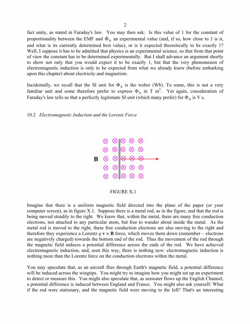
2fact unity, as stated in Faraday's law. You may then ask: Is this value of 1 for the constant of proportionality between the EMF and BΦ& an experimental value (and, if so, how close to 1 is it, and what is its currently determined best value), or is it expected theoretically to be exactly 1? Well, I suppose it has to be admitted that physics is an experimental science, so that from that point of view the constant has to be determined experimentally. But I shall advance an argument shortly to show not only that you would expect it to be exactly 1, but that the very phenomenon of electromagnetic induction is only to be expected from what we already knew (before embarking upon this chapter) about electricity and magnetism. Incidentally, we recall that the SI unit for ΦB is the weber (Wb). To some, this is not a very familiar unit and some therefore prefer to express ΦB in T m2. Yet again, consideration of Faraday's law tells us that a perfectly legitimate SI unit (which many prefer) for ΦB is V s. 10.2 Electromagnetic Induction and the Lorentz Force Imagine that there is a uniform magnetic field directed into the plane of the paper (or your computer screen), as in figure X.1. Suppose there is a metal rod, as in the figure, and that the rod is being moved steadily to the right. We know that, within the metal, there are many free conduction electrons, not attached to any particular atom, but free to wander about inside the metal. As the metal rod is moved to the right, these free conduction electrons are also moving to the right and therefore they experience a Lorentz q v % B force, which moves them down (remember – electrons are negatively charged) towards the bottom end of the rod. Thus the movement of the rod through the magnetic field induces a potential difference across the ends of the rod. We have achieved electromagnetic induction, and, seen this way, there is nothing new: electromagnetic induction is nothing more than the Lorentz force on the conduction electrons within the metal. You may speculate that, as an aircraft flies through Earth's magnetic field, a potential difference will be induced across the wingtips. You might try to imagine how you might set up an experiment to detect or measure this. You might also speculate that, as seawater flows up the English Channel, a potential difference is induced between England and France. You might also ask yourself: What if the rod were stationary, and the magnetic field were moving to the left? That's an interesting

1 1 1 1 1 1 1 1 1 1 1 1 1 1 1 1 1 1 1 1 1 1 1 1 1

FIGURE X.1

B

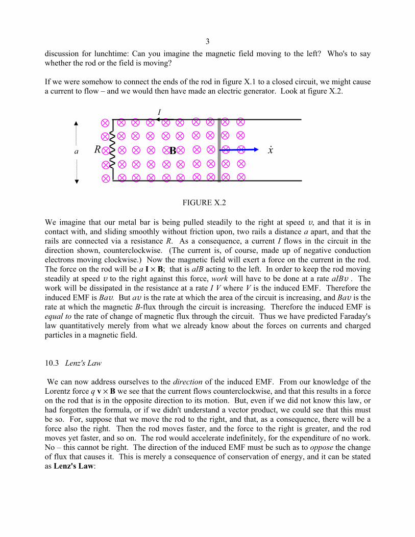
3discussion for lunchtime: Can you imagine the magnetic field moving to the left? Who's to say whether the rod or the field is moving? If we were somehow to connect the ends of the rod in figure X.1 to a closed circuit, we might cause a current to flow – and we would then have made an electric generator. Look at figure X.2. We imagine that our metal bar is being pulled steadily to the right at speed v, and that it is in contact with, and sliding smoothly without friction upon, two rails a distance a apart, and that the rails are connected via a resistance R. As a consequence, a current I flows in the circuit in the direction shown, counterclockwise. (The current is, of course, made up of negative conduction electrons moving clockwise.) Now the magnetic field will exert a force on the current in the rod. The force on the rod will be a I % B; that is aIB acting to the left. In order to keep the rod moving steadily at speed v to the right against this force, work will have to be done at a rate aIBv . The work will be dissipated in the resistance at a rate I V where V is the induced EMF. Therefore the induced EMF is Bav. But av is the rate at which the area of the circuit is increasing, and Bav is the rate at which the magnetic B-flux through the circuit is increasing. Therefore the induced EMF is equal to the rate of change of magnetic flux through the circuit. Thus we have predicted Faraday's law quantitatively merely from what we already know about the forces on currents and charged particles in a magnetic field. 10.3 Lenz's Law We can now address ourselves to the direction of the induced EMF. From our knowledge of the Lorentz force q v % B we see that the current flows counterclockwise, and that this results in a force on the rod that is in the opposite direction to its motion. But, even if we did not know this law, or had forgotten the formula, or if we didn't understand a vector product, we could see that this must be so. For, suppose that we move the rod to the right, and that, as a consequence, there will be a force also the right. Then the rod moves faster, and the force to the right is greater, and the rod moves yet faster, and so on. The rod would accelerate indefinitely, for the expenditure of no work. No – this cannot be right. The direction of the induced EMF must be such as to oppose the change of flux that causes it. This is merely a consequence of conservation of energy, and it can be stated as Lenz's Law:

FIGURE X.2

a

1 1 1 1 1 1 1 1 1 1 1 1 1 1 1 1 1 1 1 1 1 1 1 1 1

B

1 1 1 1 1 1 1 1 1 1 1 1 1 1 1 1 1 1 1 1 1 1 1 1 1

R x&

I

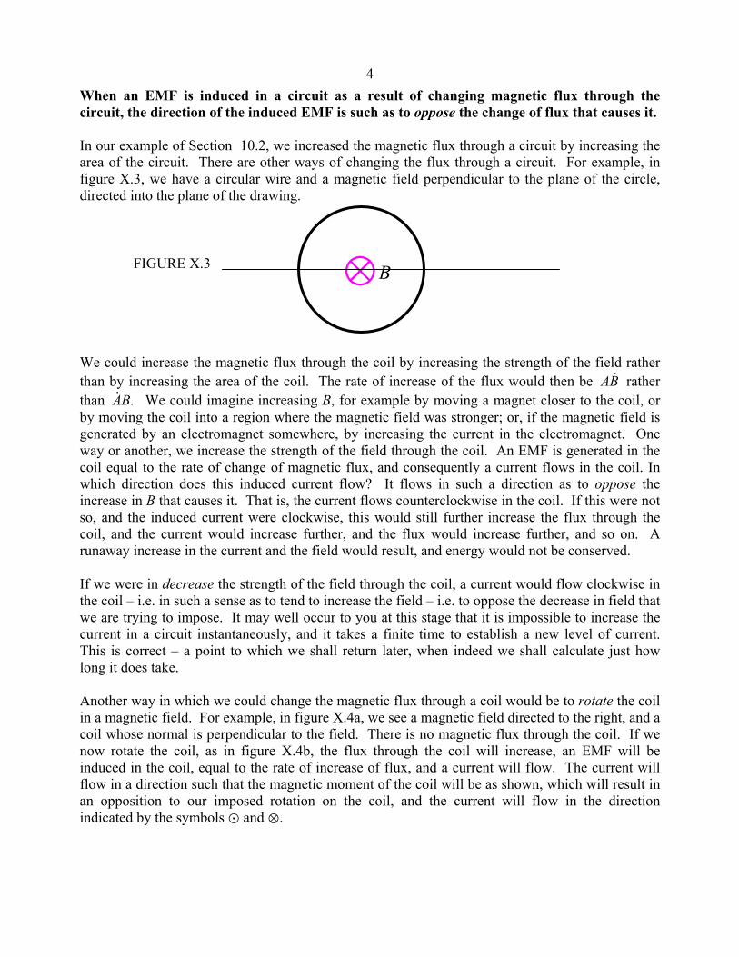
4When an EMF is induced in a circuit as a result of changing magnetic flux through the circuit, the direction of the induced EMF is such as to oppose the change of flux that causes it. In our example of Section 10.2, we increased the magnetic flux through a circuit by increasing the area of the circuit. There are other ways of changing the flux through a circuit. For example, in figure X.3, we have a circular wire and a magnetic field perpendicular to the plane of the circle, directed into the plane of the drawing. We could increase the magnetic flux through the coil by increasing the strength of the field rather than by increasing the area of the coil. The rate of increase of the flux would then be BA & rather than .BA& We could imagine increasing B, for example by moving a magnet closer to the coil, or by moving the coil into a region where the magnetic field was stronger; or, if the magnetic field is generated by an electromagnet somewhere, by increasing the current in the electromagnet. One way or another, we increase the strength of the field through the coil. An EMF is generated in the coil equal to the rate of change of magnetic flux, and consequently a current flows in the coil. In which direction does this induced current flow? It flows in such a direction as to oppose the increase in B that causes it. That is, the current flows counterclockwise in the coil. If this were not so, and the induced current were clockwise, this would still further increase the flux through the coil, and the current would increase further, and the flux would increase further, and so on. A runaway increase in the current and the field would result, and energy would not be conserved. If we were in decrease the strength of the field through the coil, a current would flow clockwise in the coil – i.e. in such a sense as to tend to increase the field – i.e. to oppose the decrease in field that we are trying to impose. It may well occur to you at this stage that it is impossible to increase the current in a circuit instantaneously, and it takes a finite time to establish a new level of current. This is correct – a point to which we shall return later, when indeed we shall calculate just how long it does take. Another way in which we could change the magnetic flux through a coil would be to rotate the coil in a magnetic field. For example, in figure X.4a, we see a magnetic field directed to the right, and a coil whose normal is perpendicular to the field. There is no magnetic flux through the coil. If we now rotate the coil, as in figure X.4b, the flux through the coil will increase, an EMF will be induced in the coil, equal to the rate of increase of flux, and a current will flow. The current will flow in a direction such that the magnetic moment of the coil will be as shown, which will result in an opposition to our imposed rotation on the coil, and the current will flow in the direction indicated by the symbols ? and 1.

FIGURE X.3 1

B

5 If the flux through a coil changes at a rate ,BΦ& and if the coil is not just a single turn but is made of N turns, the induced EMF will be BΦ& per turn, so that the induced EMF in the coil as a whole will be .BΦ&N 10.4 Ballistic Galvanometer and the Measurement of Magnetic Field A galvanometer is similar to a sensitive ammeter, differing mainly in that when no current passes through the meter, the needle is in the middle of the dial rather than at the left hand end. A galvanometer is used not so much to measure a current, but rather to detect whether or not a current is flowing, and in which direction. In the ballistic galvanometer, the motion of the needle is undamped, or as close to undamped as can easily be achieved. If a small quantity of electricity is passed through the ballistic galvanometer in a time that is short compared with the period of oscillation of the needle, the needle will jerk from its rest position, and then swing to and fro in lightly damped harmonic motion. (It would be simple harmonic motion if it could be completely undamped.) The amplitude of the motion, or rather the extent of the first swing, depends on the quantity of electricity that was passed through the galvanometer. It could be calibrated, for example, by discharging various capacitors through it, and making a table or graph of amplitude of swing versus quantity of electricity passed. Now, if we have a small coil of area A, N turns, resistance R, we could place the coil perpendicular to a magnetic field B, and then connect the coil to a ballistic galvanometer. Then, suddenly (in a time that is short compared with the oscillation period of the galvanometer), remove the coil from the field (or rotate it through 90o) so that the flux through the coil goes from AB to zero. While the

FIGURE X.4

(a) (b)

?

1

ω

6

flux through the coil is changing, and EMF will be induced, equal to ,BNA & and consequently a current will flow momentarily through the coil of magnitude ,)/( rRBNAI += & 10.4.1 where r is the resistance of the galvanometer. Integrate this with respect to time, with initial condition Q = 0 when t = 0, and we find for the total quantity of electricity that flows through the galvanometer Q NAB R r= +/( ) . 10.4.2 Since Q can be measured from the amplitude of the galvanometer motion, the strength of the magnetic field, B is determined. I mentioned that the ballistic galvanometer differs from that of an ordinary galvanometer or ammeter in that its motion is undamped. The motion of the needle in an ordinary ammeter is damped, so that the needle doesn't swing violently whenever the current is changed, and so that the needle moves promptly and purposefully towards its correct position. How is this damping achieved? The coil of a moving-coil meter is wound around a small aluminium frame called a former. When the current through the ammeter coil is changed, the coil – and the former – swing round; but a current is induced in the former, which gives the former a magnetic moment in such a sense as to oppose and therefore dampen the motion. The resistance of the former is made just right so that critical damping is achieved, so that the needle reaches its equilibrium position in the least time without overshoot or swinging. The little aluminium former does not look as if it were an important part of the instrument – but in fact its careful design is very important! 10.5 AC Generator This and the following sections will be devoted to generators and motors. I shall not be concerned with – and indeed am not knowledgeable about – the engineering design or practical details of real generators or motors, but only with the scientific principles involved. The "generators" and "motors" of this chapter will be highly idealized abstract concepts bearing little obvious resemblance to the real things. Need an engineering student, then, pay any attention to this? Well, of course, all real generators and motors obey and are designed around these very scientific principles, and they wouldn't work unless their designers and builders had a very clear knowledge and understanding of the basic principles. The rod sliding on rails in a magnetic field described in Section 10.2 in fact was a D.C. (direct current) generator. I now describe an A.C. (alternating current) generator. In figure X.5 we have a magnetic field B, and inside the field we have a coil of area A (yes – area is a vector) and N turns. The coil is being physically turned counterclockwise by some outside agency at an angular speed ω radians per second. I am not concerned with who, what or how it is

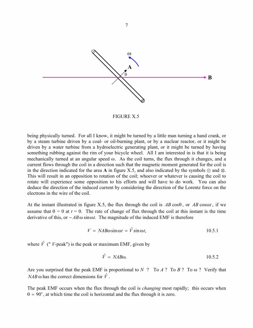
7 being physically turned. For all I know, it might be turned by a little man turning a hand crank, or by a steam turbine driven by a coal- or oil-burning plant, or by a nuclear reactor, or it might be driven by a water turbine from a hydroelectric generating plant, or it might be turned by having something rubbing against the rim of your bicycle wheel. All I am interested in is that it is being mechanically turned at an angular speed ω. As the coil turns, the flux through it changes, and a current flows through the coil in a direction such that the magnetic moment generated for the coil is in the direction indicated for the area A in figure X.5, and also indicated by the symbols ? and 1. This will result in an opposition to rotation of the coil; whoever or whatever is causing the coil to rotate will experience some opposition to his efforts and will have to do work. You can also deduce the direction of the induced current by considering the direction of the Lorentz force on the electrons in the wire of the coil. At the instant illustrated in figure X.5, the flux through the coil is AB cos ,θ or AB tcos ,ω if we assume that θ = 0 at t = 0. The rate of change of flux through the coil at this instant is the time derivative of this, or − AB tω ωsin . The magnitude of the induced EMF is therefore ,sinˆsin tVtNABV ω=ωω= 10.5.1 where V (" V-peak") is the peak or maximum EMF, given by .ˆ ω= NABV 10.5.2 Are you surprised that the peak EMF is proportional to N ? To A ? To B ? To ω ? Verify that NAB ω has the correct dimensions for V . The peak EMF occurs when the flux through the coil is changing most rapidly; this occurs when θ = 90o, at which time the coil is horizontal and the flux through it is zero.

A

?

1

ω

B θ

FIGURE X.5

8 The leads from the coil can be connected to an external circuit via a pair of slip rings through which they can deliver current to the circuit. The actual physical design of a generator is beyond the scope of this chapter and indeed of my expertise, though all depend on the physical principles herein described. In the "design" (such as it is) that I have described, the coil in which the EMF is induced is the rotor while the magnet is the stator – but this need not always be the case, and indeed designs are perfectly possible in which the magnet is the rotor and the coil the stator. In my design, too, I have assumed that there is but one coil – but there might be several in different planes. For example, you might have three coils whose planes make angles of 120o with each other. Each then generates a sinusoidal voltage, but the phase of each differs by 120o from the phases of the other two. This enables the delivery of power to three circuits. In a common arrangement these three circuits are not independent, but each is connected to a common line. The EMF in this common line is then made up three sine waves differing in phase by 120o : .)]240sin()120sin([sinˆ oo +ω++ω+ω= tttVV 10.5.3 There are several ways in which you can see what this is like. For example, you could calculate this expression for numerous values of t and plot the function out as a graph. Or you could expand the expressions V t= +sin( )ω 120o and V t= +sin( )ω 240o , and gather the various terms together to see what you get. (I recommend trying this.) Or you could simply add the three components in a phase diagram:

FIGURE X.6

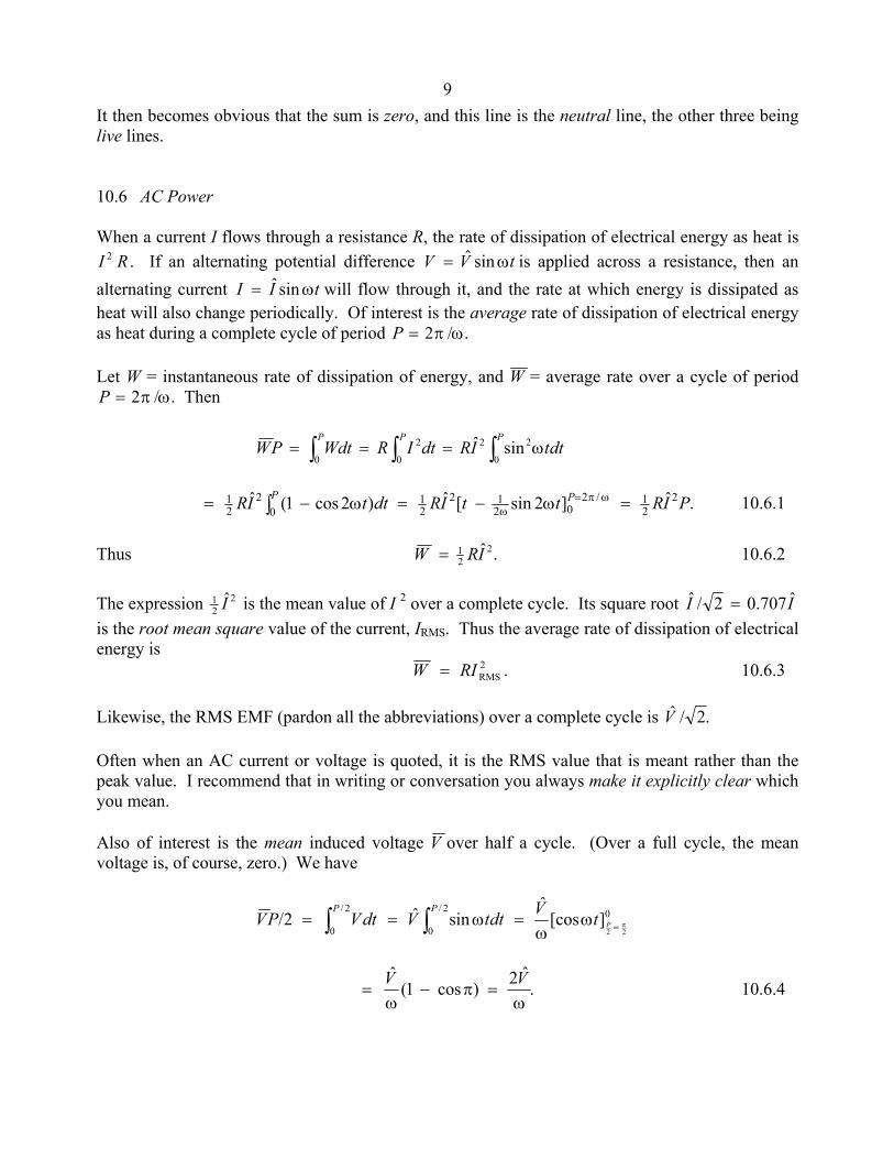
9It then becomes obvious that the sum is zero, and this line is the neutral line, the other three being live lines. 10.6 AC Power When a current I flows through a resistance R, the rate of dissipation of electrical energy as heat is I R2 . If an alternating potential difference tVV ω= sinˆ is applied across a resistance, then an alternating current tII ω= sinˆ will flow through it, and the rate at which energy is dissipated as heat will also change periodically. Of interest is the average rate of dissipation of electrical energy as heat during a complete cycle of period P = 2π ω/ . Let W = instantaneous rate of dissipation of energy, and W = average rate over a cycle of period P = 2π ω/ . Then dttIRdtIRWdtPW

PPP

∫∫∫ ω===0

22

0

2

0sinˆ

.ˆ]2sin[ˆ)2cos1(ˆ 2

21/2

0212

21

02

21 PIRttIRdttIR PP =ω−=ω−= ωπ=

ω∫ 10.6.1 Thus .ˆ2

21 IRW = 10.6.2

The expression 2

21 I is the mean value of I 2 over a complete cycle. Its square root II ˆ707.02/ˆ =

is the root mean square value of the current, IRMS. Thus the average rate of dissipation of electrical energy is W RI= RMS

2 . 10.6.3 Likewise, the RMS EMF (pardon all the abbreviations) over a complete cycle is .2/V Often when an AC current or voltage is quoted, it is the RMS value that is meant rather than the peak value. I recommend that in writing or conversation you always make it explicitly clear which you mean. Also of interest is the mean induced voltage V over half a cycle. (Over a full cycle, the mean voltage is, of course, zero.) We have

02/

0

2/

0 22][cos

ˆsinˆ2/ π=ω

ω=ω== ∫∫ PtVdttVdtVPV

PP

.ˆ2)cos1(

ˆ

ω=π−

ω=

VV 10.6.4

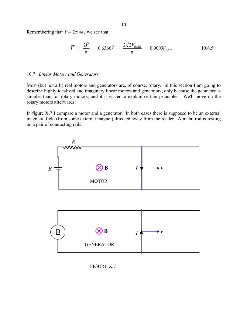
10Remembering that P = 2π ω/ , we see that

.9003.022ˆ6366.0ˆ2

RMSRMS VVVVV =

π==

π= 10.6.5

10.7 Linear Motors and Generators Most (but not all!) real motors and generators are, of course, rotary. In this section I am going to describe highly idealized and imaginary linear motors and generators, only because the geometry is simpler than for rotary motors, and it is easier to explain certain principles. We'll move on the rotary motors afterwards. In figure X.7 I compare a motor and a generator. In both cases there is supposed to be an external magnetic field (from some external magnet) directed away from the reader. A metal rod is resting on a pair of conducting rails.

1B v I

R

E

MOTOR

1B v I

GENERATOR

FIGURE X.7

B

11In the motor, a battery is connected in the circuit, causing a current to flow clockwise around the circuit. The interaction between the current and the external magnetic field produces a force on the rod, moving it to the right. In the generator, the rod is moved to the right by some externally applied force, and a current is induced counterclockwise. If the B inside the circle represents a light bulb, a current will flow through the bulb, and the bulb will light up. Let us suppose that the rails are smooth and frictionless, and suppose that, in the motor, the rod isn't pulling any weight. That is to say, suppose that there is no mechanical load on the motor. How fast will the rod move? Since there is a force moving the rod to the right, will it continue to accelerate indefinitely to the right, with no limit to its eventual speed? No, this is not what happens. When the switch is first closed and the rod is stationary, a current will flow, given by E = IR, where E is the EMF of the battery and R is the total resistance of the circuit. However, when the rod has reached a speed v, the area of the circuit is increasing at a rate av, and a back EMF (which opposes the EMF of the battery), of magnitude avB is induced, so the net EMF in the circuit is now

BaE v− and the current is correspondingly reduced according to E a B IR− =v . 10.7.6 Eventually the rod reaches a limiting speed of E aB/ ( ) , at which point no further current is being taken from the battery, and the rod (sliding as it is on frictionless rails with no mechanical load) then obeys Newton's first law of motion – namely it will continue in its state of uniform motion, because no forces are no acting upon it. Problem 1. Show that the speed increases with time according to

,)(exp12

−−=

mRtBa

aBEv 10.7.7

where m is the mass of the rod. Problem 2. Show that the time for the rod to reach half of its maximum speed is

t mRa B1 2 2

2/

ln( )

.= 10.7.8

Problem 3. Suppose that E = 120 V, a = 1.6 m , m = 1.92 kg and R = 4 Ω . If the rod reaches a speed of 300 m s−1 in 300 s, what is the strength of the magnetic field? I'll give solutions to these problems at the end of this section. Until then – no peeking.

12In a frictionless rotary motor, the situation would be similar. Initially the current would be E/R, but, when the motor is rotating with angular speed ω, the average back EMF is 2NAB ω π/ equation 10.5.5), and by the time this has reached the EMF of the battery, the frictionless, loadless coil carries on rotating at constant angular speed, taking no current from the battery. Now let's go back to our linear motor consisting of a metal rod lying on two rails, but this time suppose that there is some mechanical resistance to the motion. This could be either because there is friction between the rod and the rails, or perhaps the rod is dragging a heavy weight behind it, or both. One way or another, let us suppose that the rod is subjected to a constant force F towards the left. As before, the relation between the current and the speed is given by equation 10.7.6, but, when a steady state has been reached, the electromagnetic force aIB pulling the rod to the right is equal to the mechanical load F dragging the rod to the left. That is, E a B IR− =v and F a I B= . If we eliminate I between these two equations, we obtain

E a B FRaB

− =v , 10.7.9

or v = −E

a BR

a BF

( ).2 10.7.10

This equation, which relates the speed at which the motor runs to the mechanical load, is called the motor performance characteristic. In our particular motor, the performance characteristic shows that the speed at which the motor runs decreases steadily as the load is increased., and the motor runs to a grinding halt for a load equal to a B E R/ . (Verify that this has the dimensions of force.) The current is then E/R. This current may be quite large. If you physically prevent a real motor from turning by applying a mechanical torque to it so large that the motor cannot move, a large current will flow through the coil – large enough to heat and possibly fuse the coil. You will hear a sharp crack and see a little puff of smoke. If we multiply equation 10.7.6 by I, we obtain E I a I B I R= +v 2 , 10.7.11 or E I F I R= +v 2 . 10.7.12 This shows that the power produced by the battery goes partly into doing external mechanical work, and the remainder is dissipated as heat in the resistance. Restrain the motor so that v = 0, and all of that E I goes into I 2R. If you were physically to move the rod to the right at a speed faster than the equilibrium speed, the back EMF becomes greater than the battery EMF, and current flows back into the battery. The device is then a generator rather than a motor. The nature of the performance characteristic varies with the details of motor design. You may not want a motor whose speed decreases so drastically with load. You may have to decide in advance

13what sort of performance characteristic you want the motor to have, depending on what tasks you want it to perform, and then you have to design the motor accordingly. We shall mention some possibilities in the next section. Now – the promised solutions to the problems. Solution to Problem 1. When the speed of the rod is v, the net EMF in the circuit is E a B− v , so the current is( ) /E a B R− v , and so the force on the rod will be aB E a B R( ) /− v and the acceleration d dtv / will be aB E a B mR( ) /( ) .− v The equation of motion is therefore

.dtmRaB

aBEd

=− v

v 10.7.13

Integration, with v = 0 when t = 0, gives the required equation 10.7.7. Solution to Problem 2.

Just put v =Ea B2

in equation 10.7.7 and solve for t. Verify that the expression has the dimensions

of time. Solution to Problem 3. Put the given numbers into equation 10.7.7 to get B e B= − −1

41001

2

( ) 10.7.14 and solve this for B. (Nice and easy. But if you are not experienced in solving equations such as this, the Newton-Raphson process is described in Chapter 1 of the Celestial Mechanics notes of this series. This equation would be good practice.) There are two possible answers, namely 0.043996 T and 0.249505 teslas. I draw the speed:time graphs for the two solutions below:

14

0 500 1000 15000

200

400

600

800

1000

1200

Time s

Spe

ed m

s-1

Numbers of interest for the two fields: B (T) ∞v (m s−1) t s 0.0440 1704.7 1074.29 0.2495 300.6 33.40 10.8 Rotary Motors Most real motors, of course, are rotary motors, though all of the principles described for our highly idealized linear motor of the previous section still apply. Current is fed into a coil (known as the armature) via a split-ring commutator and the coil therefore develops a magnetic moment. The coil is in a magnetic field, and it therefore experiences a torque. (Figure X.5) The coil rotates and soon its magnetic moment vector will be parallel to the field and there would be no further torque – except that, at that instant, the split-ring commutator reverses the direction of the current in the coil, and hence reverses the direction of the magnetic moment. Thus the coil continues to rotate until, half a period later, its new magnetic moment again lines up with the magnetic field, and the commutator again reverses the direction of the moment.

15As in the case of the linear motor, the coil reaches a maximum angular speed, which depends on the mechanical load (this time a torque). and the relation between the maximum angular speed and the torque is the motor performance characteristic. Also, as with a generator, there may be several coils (with a corresponding number of sections in the commutator), and it is also possible to design motors in which the armature is the stator and the magnet the rotor – but I am not particularly knowledgeable about the detailed engineering designs of real motors – except that all of them depend upon the same scientific principles. In all of the foregoing, it has been assumed that the magnetic field is constant, as if produced by a permanent magnet. In real motors, the field is generally produced by an electromagnet. (Some types of iron retain their magnetism permanently unless deliberately demagnetized. Others become magnetized only when placed in a strong magnetic field such as produced by a solenoid, and they lose most of their magnetization as soon as the magnetizing field is removed.) The field coils may be wound in series with the armature coil (a series-wound motor) or in parallel with it (a shunt-wound motor), or even partly in series and partly in parallel (a compound-wound motor). Each design has it own performance characteristic, depending on the use for which it is intended. With a single coil rotating in a magnetic field, the induced back EMF varies periodically, the average value being, as we have seen, 2 NAB ω π/ . In practice the coil may be wound around many slots placed around the perimeter of a cylindrical core every few degrees, and there are a corresponding number of sections in the split-ring commutator. The back EMF is then less variable than with a single coil, and, although the formula 2 NAB ω π/ is no longer appropriate, the back EMF is still proportional to B ω. We can write the average back EMF as KBω, where the motor constant K depends on the detailed geometry of a particular design. Shunt-wound Motor. In the shunt-wound motor, the field coil is wound in parallel to the armature coil. In this case, the back EMF generated in the armature does not affect the current in the field coil, so the motor operates rather as previously described for a constant field. That is, the motor performance characteristic, giving the equilibrium angular speed in terms of the mechanical load (torque, τ) is given by

ω τ= −E

KBR

KB( ).

2 10.8.1

Here, R is the armature resistance. In practice, there may be a variable resistance (rheostat) in series with the field coil, so that the current through the field coil – and hence the field strength – can be changed. Series-wound Motor. The field coil is wound in series with the armature, and the motor performance characteristic is rather different that for the shunt-wound motor. If the magnet core does not saturate, then, to a linear approximation, the field is proportional to the current, and the back EMF is proportional to the product of the current I and the angular speed ω - so let's say that the back EMF is kIω. We then have

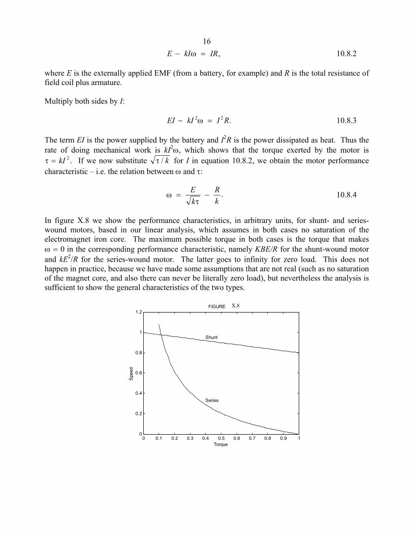
16 E kI IR− =ω , 10.8.2 where E is the externally applied EMF (from a battery, for example) and R is the total resistance of field coil plus armature. Multiply both sides by I: EI kI I R− =2 2ω . 10.8.3 The term EI is the power supplied by the battery and I2R is the power dissipated as heat. Thus the rate of doing mechanical work is kI2ω, which shows that the torque exerted by the motor is τ = kI 2 . If we now substitute τ / k for I in equation 10.8.2, we obtain the motor performance characteristic – i.e. the relation between ω and τ:

ωτ

= −Ek

Rk

. 10.8.4

In figure X.8 we show the performance characteristics, in arbitrary units, for shunt- and series-wound motors, based in our linear analysis, which assumes in both cases no saturation of the electromagnet iron core. The maximum possible torque in both cases is the torque that makes ω = 0 in the corresponding performance characteristic, namely KBE/R for the shunt-wound motor and kE2/R for the series-wound motor. The latter goes to infinity for zero load. This does not happen in practice, because we have made some assumptions that are not real (such as no saturation of the magnet core, and also there can never be literally zero load), but nevertheless the analysis is sufficient to show the general characteristics of the two types.

0 0.1 0.2 0.3 0.4 0.5 0.6 0.7 0.8 0.9 1

0

0.2

0.4

0.6

0.8

1

1.2

Spe

ed

Torque

FIGURE X.7

Shunt

Series

X.8

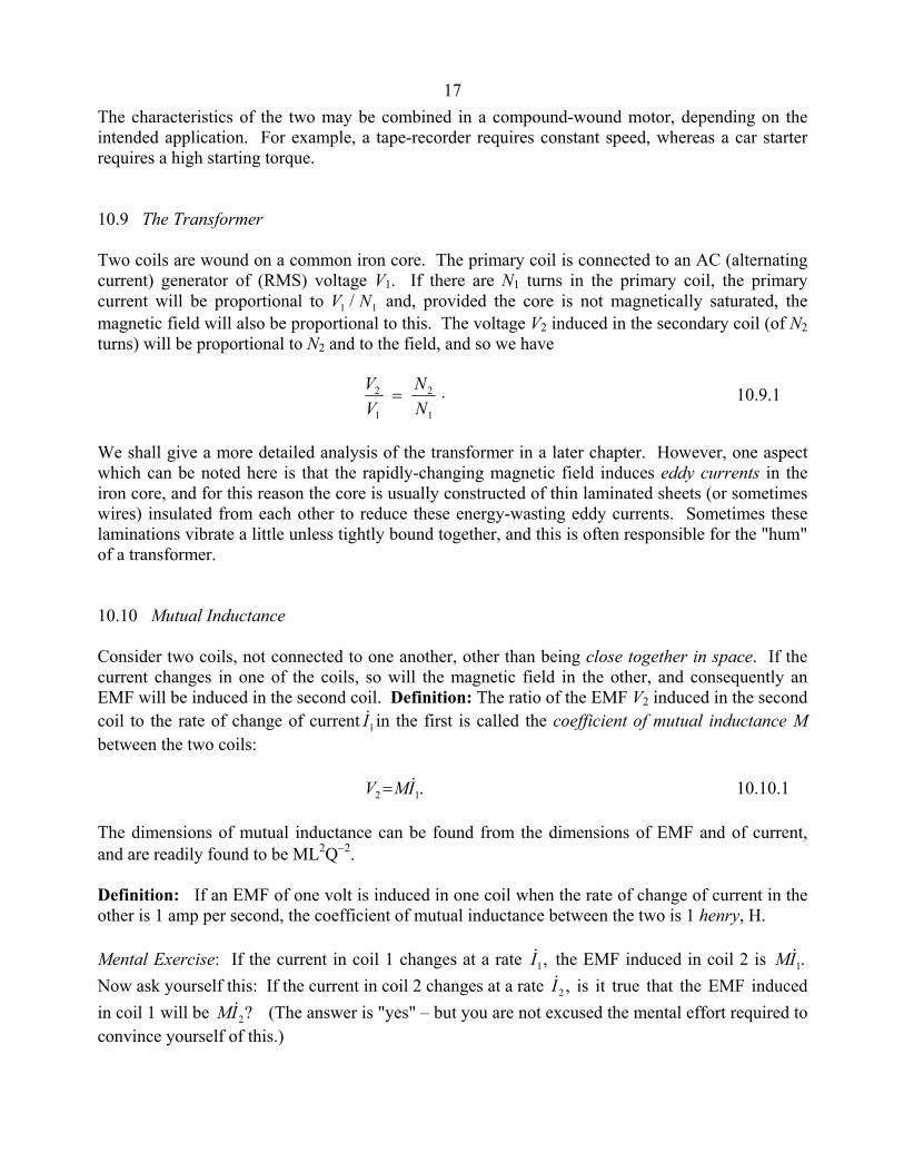
17The characteristics of the two may be combined in a compound-wound motor, depending on the intended application. For example, a tape-recorder requires constant speed, whereas a car starter requires a high starting torque. 10.9 The Transformer Two coils are wound on a common iron core. The primary coil is connected to an AC (alternating current) generator of (RMS) voltage V1. If there are N1 turns in the primary coil, the primary current will be proportional to V N1 1/ and, provided the core is not magnetically saturated, the magnetic field will also be proportional to this. The voltage V2 induced in the secondary coil (of N2 turns) will be proportional to N2 and to the field, and so we have

VV

NN

2

1

2

1

= . 10.9.1

We shall give a more detailed analysis of the transformer in a later chapter. However, one aspect which can be noted here is that the rapidly-changing magnetic field induces eddy currents in the iron core, and for this reason the core is usually constructed of thin laminated sheets (or sometimes wires) insulated from each other to reduce these energy-wasting eddy currents. Sometimes these laminations vibrate a little unless tightly bound together, and this is often responsible for the "hum" of a transformer. 10.10 Mutual Inductance Consider two coils, not connected to one another, other than being close together in space. If the current changes in one of the coils, so will the magnetic field in the other, and consequently an EMF will be induced in the second coil. Definition: The ratio of the EMF V2 induced in the second coil to the rate of change of current 1I& in the first is called the coefficient of mutual inductance M between the two coils: .12 IMV &= 10.10.1 The dimensions of mutual inductance can be found from the dimensions of EMF and of current, and are readily found to be ML2Q−2. Definition: If an EMF of one volt is induced in one coil when the rate of change of current in the other is 1 amp per second, the coefficient of mutual inductance between the two is 1 henry, H. Mental Exercise: If the current in coil 1 changes at a rate ,1I& the EMF induced in coil 2 is .1IM & Now ask yourself this: If the current in coil 2 changes at a rate ,2I& is it true that the EMF induced in coil 1 will be ?2IM & (The answer is "yes" – but you are not excused the mental effort required to convince yourself of this.)

18 Example: Suppose that the primary coil is an infinite solenoid having n1 turns per unit length wound round a core of permeability µ. Tightly would around this is a plain circular coil of N2 turns. The solenoid and the coil wrapped tightly round it are of area A. We can calculate the mutual inductance of this arrangement as follows. The magnetic field in the primary is µn1I so the flux through each coil is µn1AI. If the current changes at a rate ,I& flux will change at a rate ,InA &µ and the EMF induced in the secondary coil will be .21 IANn &µ Therefore the mutual inductance is M n N A= µ 1 2 . 10.10.2 Several points: 1. Verify that this has the correct dimensions. 2 If the current in the solenoid changes in such a manner as to cause an increase in the magnetic

field towards the right, the EMF induced in the secondary coil is such that, if it were connected to a closed circuit so that a secondary current flows, the direction of this current will produce a magnetic field towards the left – i.e. such as to oppose the rightward increase in B.

3. Because of the little mental effort you made a few minutes ago, you are now convinced that, if

you were to change the current in the plane coil at a rate ,I& the EMF induced in the solenoid would be ,IM & where M is given by equation 10.10.2.

4. Equation 10.10.2 is the equation for the mutual inductance of the system, provided that the coil and the solenoid are tightly coupled. If the coil is rather loosely draped around the solenoid, or if the solenoid is not infinite in length, the mutual inductance would be rather less than given by equation 10.10.2. It would be, in fact, k n N Aµ 1 2 , where k, a dimensionless number between 0 and 1, is the coupling coefficient.

5. While we have hitherto expressed permeability in units of tesla metres per amp (T m A−1) or

some such combination, equation 10.10.2 shows that permeability can equally well be (and usually is) expressed in henrys per metre, H m−1. Thus, we say that the permeability of free space is µ π0

7 14 10= × − −H m . Exercise: A plane coil of 10 turns is tightly wound around a solenoid of diameter 2 cm having 400 turns per centimetre. The relative permeability of the core is 800. Calculate the mutual inductance. (I make it 0.126 H.) 10.11 Self Inductance In this section we are dealing with the self inductance of a single coil rather than the mutual inductance between two coils. If the current through a single coil changes, the magnetic field inside that coil will change; consequently a back EMF will be induced in the coil that will oppose the change in the magnetic field and indeed will oppose the change of current. Definition: The ratio of

19the back EMF to the rate of change of current is the coefficient of self inductance L. If the back EMF is 1 volt when the current changes at a rate of one amp per metre, the coefficient of self inductance is 1 henry. Exercise: Show that the coefficient of self inductance (usually called simply the "inductance") of a long solenoid of length l and having n turns per unit length is µn Al2 , where I'm sure you know what all the symbols stand for. Put some numbers in for an imaginary solenoid of your own choosing, and calculate its inductance in henrys. The circuit symbol for inductance is If a coil has an iron core, this may be indicated in the circuit by The symbol for a transformer is Finally, don't confuse self-inductance with self-indulgence. 10.12 Growth of Current in a Circuit Containing Inductance It will have occurred to you that if the growth of current in a coil results in a back EMF which opposes the increase of current, current cannot change instantaneously in a circuit that contains inductance. This is correct. (Recall also that the potential difference in a circuit cannot change instantaneously in a circuit containing capacitance. Come to think of it, it is hardly possible for the capacitance or inductance of any circuit to be exactly zero; any real circuit must have some capacitance and inductance, even if very small.) Consider the circuit of figure X.9. A battery of EMF E is in series with a resistance and an inductance. (A coil or solenoid or any inductor in general will have both inductance and resistance, so the R and the L in the figure may belong to one single item.) We have to be very careful about signs in what follows.

FIGURE X.9 II &,

E

R L

IL &

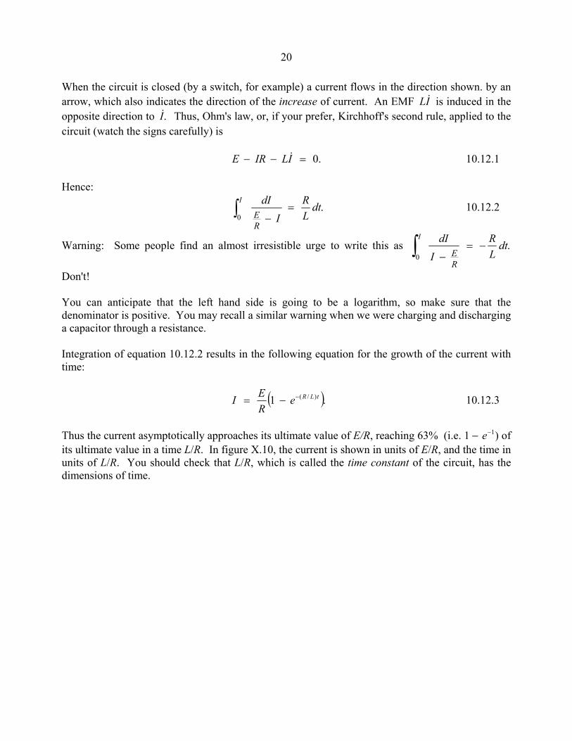
20 When the circuit is closed (by a switch, for example) a current flows in the direction shown. by an arrow, which also indicates the direction of the increase of current. An EMF IL & is induced in the opposite direction to .I& Thus, Ohm's law, or, if your prefer, Kirchhoff's second rule, applied to the circuit (watch the signs carefully) is .0=−− ILIRE & 10.12.1 Hence:

.0

dtLR

IdI

RE

I=

−∫ 10.12.2

Warning: Some people find an almost irresistible urge to write this as .0

dtLR

IdI

RE

I−=

−∫

Don't! You can anticipate that the left hand side is going to be a logarithm, so make sure that the denominator is positive. You may recall a similar warning when we were charging and discharging a capacitor through a resistance. Integration of equation 10.12.2 results in the following equation for the growth of the current with time:

( ).1 )/( tLReREI −−= 10.12.3

Thus the current asymptotically approaches its ultimate value of E/R, reaching 63% (i.e. 1 1− −e ) of its ultimate value in a time L/R. In figure X.10, the current is shown in units of E/R, and the time in units of L/R. You should check that L/R, which is called the time constant of the circuit, has the dimensions of time.

21

0 0.5 1 1.5 2 2.5

0

0.1

0.2

0.3

0.4

0.5

0.6

0.7

0.8

0.9

1

Time

Cur

rent

FIGURE X.10

10.13 Discharge of a Capacitor through an Inductance The circuit is shown in figure X.11, and, once again, it is important to take care with the signs. If +Q is the charge on the left hand plate of the capacitor at some time (and −Q the charge on the right hand plate) the current I in the direction indicated is Q&− and the potential difference across the plates is Q/C. The back EMF is in the direction shown, and we have

,0=− ILCQ & 10.13.1

or .0=+ QLCQ && 10.13.2

C

FIGURE X.11

L

IL &I

22

This can be written ,LCQQ −=&& 10.13.3

which is simple harmonic motion of period 2π LC . (verify that this has dimensions of time.) Thus energy sloshes to and fro between storage as charge in the capacitor and storage as current in the inductor. If there is resistance in the circuit, the oscillatory motion will be damped, the charge and current eventually approaching zero. But, even if there is no resistance, the oscillation does not continue for ever. While the details are beyond the scope of this chapter, being more readily dealt with in a discussion of electromagnetic radiation, the periodic changes in the charge in the capacitor and the current in the inductor, result in an oscillating electromagnetic field around the circuit, and in the generation of an electromagnetic wave, which carries energy away at a speed of 1 0 0/ ( ) .µ ε Verify that this has the dimensions of speed, and that it has the value 2.998 % 108 m s−1. The motion in the circuit is damped just as if there were a resistance of )/(1/ 0000 ε=µ=εµ cc in the circuit. Verify that this has the dimensions of resistance and that it has a value of 376.7 Ω. This effective resistance is called the impedance of free space. 10.14 Discharge of a Capacitor through an Inductance and a Resistance This results in damped oscillatory motion. It is discussed in detail in Chapter 11 of the Classical Mechanics part of these notes, especially Section 11.6. 10.15 Energy Stored in an Inductance During the growth of the current in an inductor, at a time when the current is i and the rate of increase of current is i&, there will be a back EMF .iL& The rate of doing work against this back EMF is then .iLi& The work done in time dt is ,diLidtiLi =& where di is the increase in current in time dt. The total work done when the current is increased from 0 to I is

,221

0LIdiiL

I=∫ 10.15.1

and this is the energy stored in the inductance. (Verify the dimensions.) 10.16 Energy Stored in a Magnetic Field Recall your derivation (Section 10.11) that the inductance of a long solenoid is µn Al2 . The energy stored in it, then, is 1

22 2µn AlI . The volume of the solenoid is Al, and the magnetic field is

B n I H n I= =µ , .or Thus we find that the energy stored per unit volume in a magnetic field is

23

B BH H2

12

12

2

2µµ= = . 10.16.2

In a vacuum, the energy stored per unit volume in a magnetic field is 1

2 02µ H - even though the

vacuum is absolutely empty! Equation 10.16.2 is valid in any isotropic medium, including a vacuum. In an anisotropic medium, B and H are not in general parallel – unless they are both parallel to a crystallographic axis. More generally, in an anisotropic medium, the energy per unit volume is 1

2 B H• . Verify that the product of B and H has the dimensions of energy per unit volume.

1

CHAPTER 11 DIMENSIONS

Although we have not yet met all of the quantities in use in electricity and magnetism, we have met most of the important ones. Of those yet to come, some, such as impedance and reactance, will obviously have the dimensions of resistance; some, such as reluctance and permeance, you will rarely come across; and some, such as magnetic susceptibility, will obviously be dimensionless. Now is therefore quite a convenient time to gather together the various quantities we have come across, together with their dimensions (i.e. the powers of M, L, T and Q of which they are composed) and their SI units. It will be a good time, too, for the reader to review the definitions of the various quantities and to verify, from their definitions, their dimensions. Let me know ([email protected]) if you find any mistakes in the following table.

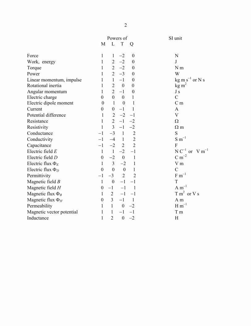
2 Powers of SI unit M L T Q Force 1 1 −2 0 N Work, energy 1 2 −2 0 J Torque 1 2 −2 0 N m Power 1 2 −3 0 W Linear momentum, impulse 1 1 −1 0 kg m s−1 or N s Rotational inertia 1 2 0 0 kg m2

Angular momentum 1 2 −1 0 J s Electric charge 0 0 0 1 C Electric dipole moment 0 1 0 1 C m Current 0 0 −1 1 A Potential difference 1 2 −2 −1 V Resistance 1 2 −1 −2 Ω Resistivity 1 3 −1 −2 Ω m Conductance −1 −3 1 2 S Conductivity −1 −4 1 2 S m−1 Capacitance −1 −2 2 2 F Electric field E 1 1 −2 −1 N C−1 or V m−1

Electric field D 0 −2 0 1 C m−2

Electric flux ΦE 1 3 −2 1 V m Electric flux ΦD 0 0 0 1 C Permittivity −1 −3 2 2 F m−1 Magnetic field B 1 0 −1 −1 T Magnetic field H 0 −1 −1 1 A m−1 Magnetic flux ΦB 1 2 −1 −1 T m2 or V s Magnetic flux ΦH 0 3 −1 1 A m Permeability 1 1 0 −2 H m−1 Magnetic vector potential 1 1 −1 −1 T m Inductance 1 2 0 −2 H

1CHAPTER 12

PROPERTIES OF MAGNETIC MATERIALS

12.1 Introduction This chapter is likely to be a short one, not least because it is a subject in which my own knowledge is, to put it charitably, a little limited. A thorough understanding of why some materials are magnetic requires a full course in the physics of the solid state, a course that I could not possibly give. Nevertheless, there are a few basic concepts and ideas concerned with magnetic materials which everyone who is interested in electromagnetism should know, and it is the aim of this chapter to describe them in a very introductory way. It may be worthwhile to remind ourselves of the ways in which we have defined the magnetic fields B and H. To define B, we noted that an electric current situated in a magnetic field experiences a force at right angles to the current, the magnitude and direction of this force depending on the direction of the current. We accordingly defined B as being equal to the maximum force per unit length experienced per unit current, the defining equation being F' = I %B. Later, we asked ourselves about the strength of the magnetic field in the vicinity of an electric current. We introduced the Biot-Savart law, which says that the contribution to the magnetic field from an element ds of a circuit carrying a current I is proportional to ( sin ) / ,I ds rθ 2 and we called the constant of proportionality µ π/ ( ),4 where µ is the permeability of the material surrounding the current. We might equally well have approached it from another angle. For example, we might have noted that the magnetic field inside a solenoid is proportional to nI, and we could have denoted the constant of proportionality µ, the permeability of the material inside the solenoid. We then defined H as being an alternative measure of the magnetic field, given by H = B/µ. In an isotropic medium, the vectors B and H are parallel, and the permeability is a scalar quantity. In an anisotropic crystal, B and H are not necessarily parallel, and the permeability is a tensor. Some people see an analogy between the equation between the equation B = µH and the equation D E= ε of electric fields. With our approach, however, I think most readers will see that, to the extent that there may be an analogy, the analogy is between D = εE and H = B/µ. For example, consider a long solenoid, in the inside of which are two different magnetic materials in series, the first of permeability µ1 and the second of greater permeability µ2. The H-field everywhere inside the solenoid is just nI, regardless of what is inside it. Like D, the component of H perpendicular to the boundary between two media is continuous, whereas the perpendicular component of B is greater inside the material with the larger permeability. Likewise, if you were to consider, for example, two different media lying side-by-side in parallel, between the poles, for example, of a horseshoe magnet, the component of B parallel to the boundary between the media is continuous, and the parallel component of H is less in the medium of greater permeability. In this chapter, we shall introduce a few new words, such as permeance and magnetization. We shall describe in a rather simple and introductory way five types of magnetism exhibited by various

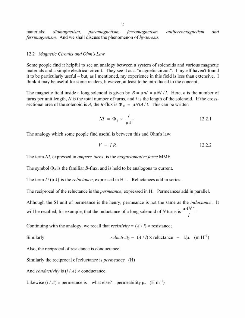
2materials: diamagnetism, paramagnetism, ferromagnetism, antiferromagnetism and ferrimagnetism. And we shall discuss the phenomenon of hysteresis. 12.2 Magnetic Circuits and Ohm's Law Some people find it helpful to see an analogy between a system of solenoids and various magnetic materials and a simple electrical circuit. They see it as a "magnetic circuit". I myself haven't found it to be particularly useful – but, as I mentioned, my experience in this field is less than extensive. I think it may be useful for some readers, however, at least to be introduced to the concept. The magnetic field inside a long solenoid is given by B nI NI l= =µ µ / . Here, n is the number of turns per unit length, N is the total number of turns, and l is the length of the solenoid. If the cross-sectional area of the solenoid is A, the B-flux is ΦB NIA l= µ / . This can be written

NI lAB= ×Φ

µ. 12.2.1

The analogy which some people find useful is between this and Ohm's law: V I R= . 12.2.2 The term NI, expressed in ampere-turns, is the magnetomotive force MMF. The symbol ΦB is the familiar B-flux, and is held to be analogous to current. The term l A/ ( )µ is the reluctance, expressed in H−1. Reluctances add in series. The reciprocal of the reluctance is the permeance, expressed in H. Permeances add in parallel. Although the SI unit of permeance is the henry, permeance is not the same as the inductance. It

will be recalled, for example, that the inductance of a long solenoid of N turns is µANl

2.

Continuing with the analogy, we recall that resistivity = (A / l) % resistance; Similarly reluctivity = (A / l) % reluctance = 1/µ. (m H−1) Also, the reciprocal of resistance is conductance. Similarly the reciprocal of reluctance is permeance. (H) And conductivity is (l / A) % conductance. Likewise (l / A) % permeance is – what else? – permeability µ. (H m−1)

3 I have mentioned these names partly for completeness and partly because it's fun to write some unusual and unfamiliar words such as permeance and reluctivity. I am probably not going to use these concepts further or give examples of their use. This is mostly because I am not as familiar with them myself as perhaps I ought to be, and I am sure that there are contexts in which these concepts are indeed highly useful. The next section introduces some more funny words, such as magnetization and susceptibility – but these are words that you will need to know and understand. 12.3 Magnetization and Susceptibility The H-field inside a long solenoid is nI. If there is a vacuum inside the solenoid, the B-field is µ µ0 0H nI= . If we now place an iron rod of permeability µ inside the solenoid, this doesn't change H, which remains nI . The B-field, however, is now B H= µ . This is greater than µ0H, and we can write

B H M= +µ0 ( ) . 12.3.1

The quantity M is called the magnetization of the material. In SI units it is expressed in A m−1. We see that there are two components to B. There is the µ µ0 0H nI= , which is the externally imposed field, and the component µ0M, originating as a result of something that has happened within the material. It might have occurred to you that you would have preferred to define the magnetization from B = µ0H + M, so that the magnetization would be the excess of B over µ0H. The equation B = µ0H + M, would be analogous to the familiar D E P= +ε0 , and the magnetization would then be expressed in tesla rather than in A m−1 . This viewpoint does indeed have much to commend it, but so does B H M= +µ0 ( ) . The latter is the recommended definition in the SI approach, and that is what we shall use here. The ratio of the magnetization M ("the result") to H ("the cause"), which is obviously a measure of how susceptible the material is to becoming magnetized, is called the magnetic susceptibility χm of the material: M H= χm . 12.3.2 On combining this with equation 12.3.1 and B = µH, we readily see that the magnetic susceptibility (which is dimensionless) is related to the relative permeability µ µ µr = / 0 by µ χr = +1 m. 12.3.3

412.4 Diamagnetism We mentioned in Section 12.1 that there are five types of magnetism exhibited by various materials. In this section we deal with the first of these, namely, diamagnetism. Diamagnetic materials have a very weak negative susceptibility, typically of order −10−6. That is to say, the relative permeability is slightly less than 1. Consequently, when a diamagnetic material is placed in a magnetic field, B H< µ0 . If you are now hearing about this phenomenon for the first time, you may be a little surprised, and you will be expecting me to present a very short list of quite exotic materials known to be diamagnetic. So, here comes a further surprise: All materials are diamagnetic. Some materials may also be paramagnetic or ferromagnetic, and their positive paramagnetic or ferromagnetic susceptibilities may be larger than their negative diamagnetic susceptibility, so that their overall susceptibility is positive. But all materials are diamagnetic, even if their diamagnetism is hidden by their greater para- or ferromagnetism. A proper account of the mechanism at the atomic level of the cause of diamagnetism requires a quantum mechanical treatment, but we can understand the phenomenon qualitatively classically. We just have to think of an atom as being a nucleus surrounded by electrons moving in orbits around the nucleus. When an atom (or a large collection of atoms in a macroscopic sample of matter) is placed in a magnetic field, a current is induced within the atom by electromagnetic induction. That is, the electrons are caused to orbit around the nucleus, and hence to give the atom a magnetic moment, in such a direction as to oppose the increase in the magnetic field that causes it. The result of this happening to all of the atoms in a macroscopic sample is that B will now be less than µ0H, and the susceptibility will be negative. But, you may argue, these induced currents and their associated opposing magnetic moments will last only so long as the external field is changing. In fact it persists as long as the magnetizing field persists. The reason is as follows. In Chapter 10, we were dealing with wires and coils and resistors, and any current induced by a changing magnetic field was rapidly dissipated. For an electron in an orbit around a nucleus, however, there is no resistance, so, once it is set in motion, it will stay in motion. The same situation would arise if we were to induce a current in a loop of wire made of superconducting material whose resistance is zero. The current, once induced, continues, and is not dissipated away as heat. 12.5 Paramagnetism Diamagnetism makes itself evident in atoms and molecules that have no permanent magnetic moment. Some atoms or molecules, however, do have a permanent magnetic moment, and such materials are paramagnetic. They must still be diamagnetic, but often the paramagnetism will outweigh the diamagnetism. The magnetic moment of an atom of a molecule is typically if order of a Bohr magneton. (See Chapter VII, Sections 21-23, of Stellar Atmospheres for more details about the Bohr magneton and the magnetic moments of atoms. All that we need note here is that a Bohr magneton is about 9.3 % 10−24 N m T−1.) The presence of a permanent magnetic moment is often the result of unpaired electron spins. An example often quoted is the oxygen molecule O2. Liquid

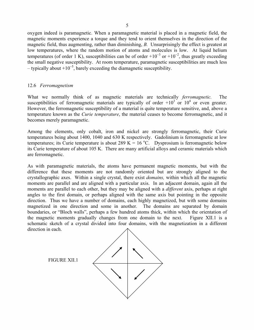
5oxygen indeed is paramagnetic. When a paramagnetic material is placed in a magnetic field, the magnetic moments experience a torque and they tend to orient themselves in the direction of the magnetic field, thus augmenting, rather than diminishing, B. Unsurprisingly the effect is greatest at low temperatures, where the random motion of atoms and molecules is low. At liquid helium temperatures (of order 1 K), susceptibilities can be of order +10−3 or +10−2, thus greatly exceeding the small negative susceptibility. At room temperature, paramagnetic susceptibilities are much less – typically about +10−5, barely exceeding the diamagnetic susceptibility. 12.6 Ferromagnetism What we normally think of as magnetic materials are technically ferromagnetic. The susceptibilities of ferromagnetic materials are typically of order +103 or 104 or even greater. However, the ferromagnetic susceptibility of a material is quite temperature sensitive, and, above a temperature known as the Curie temperature, the material ceases to become ferromagnetic, and it becomes merely paramagnetic. Among the elements, only cobalt, iron and nickel are strongly ferromagnetic, their Curie temperatures being about 1400, 1040 and 630 K respectively. Gadolinium is ferromagnetic at low temperatures; its Curie temperature is about 289 K = 16 oC. Dysprosium is ferromagnetic below its Curie temperature of about 105 K. There are many artificial alloys and ceramic materials which are ferromagnetic. As with paramagnetic materials, the atoms have permanent magnetic moments, but with the difference that these moments are not randomly oriented but are strongly aligned to the crystallographic axes. Within a single crystal, there exist domains, within which all the magnetic moments are parallel and are aligned with a particular axis. In an adjacent domain, again all the moments are parallel to each other, but they may be aligned with a different axis, perhaps at right angles to the first domain, or perhaps aligned with the same axis but pointing in the opposite direction. Thus we have a number of domains, each highly magnetized, but with some domains magnetized in one direction and some in another. The domains are separated by domain boundaries, or “Bloch walls”, perhaps a few hundred atoms thick, within which the orientation of the magnetic moments gradually changes from one domain to the next. Figure XII.1 is a schematic sketch of a crystal divided into four domains, with the magnetization in a different direction in each.

FIGURE XII.1

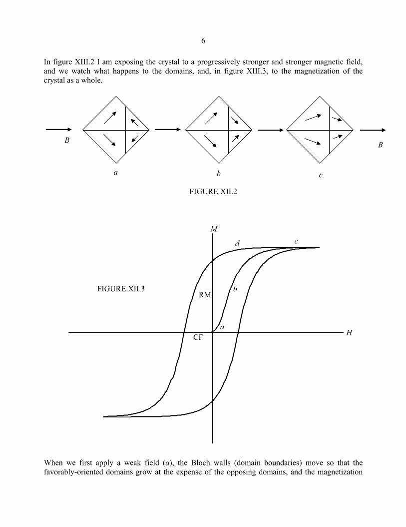
6 In figure XIII.2 I am exposing the crystal to a progressively stronger and stronger magnetic field, and we watch what happens to the domains, and, in figure XIII.3, to the magnetization of the crystal as a whole.

When we first apply a weak field (a), the Bloch walls (domain boundaries) move so that the favorably-oriented domains grow at the expense of the opposing domains, and the magnetization

B B

FIGURE XII.2

b a c

b

a

c

FIGURE XII.3

M

H

d

RM

CF

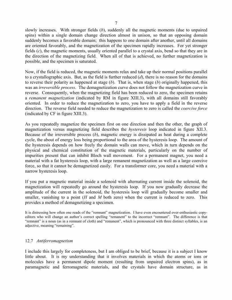
7slowly increases. With stronger fields (b), suddenly all the magnetic moments (due to unpaired spins) within a single domain change direction almost in unison, so that an opposing domain suddenly becomes a favorable domain; this happens to one domain after another, until all domains are oriented favorably, and the magnetization of the specimen rapidly increases. For yet stronger fields (c), the magnetic moments, usually oriented parallel to a crystal axis, bend so that they are in the direction of the magnetizing field. When all of that is achieved, no further magnetization is possible, and the specimen is saturated. Now, if the field is reduced, the magnetic moments relax and take up their normal positions parallel to a crystallographic axis. But, as the field is further reduced (d), there is no reason for the domains to reverse their polarity as happened at stage (b). That is, when stage (b) originally happened, this was an irreversible process. The demagnetization curve does not follow the magnetization curve in reverse. Consequently, when the magnetizing field has been reduced to zero, the specimen retains a remanent magnetization (indicated by RM in figure XIII.3), with all domains still favorably oriented. In order to reduce the magnetization to zero, you have to apply a field in the reverse direction. The reverse field needed to reduce the magnetization to zero is called the coercive force (indicated by CF in figure XIII.3). As you repeatedly magnetize the specimen first on one direction and then the other, the graph of magnetization versus magnetizing field describes the hysteresis loop indicated in figure XII.3. Because of the irreversible process (b), magnetic energy is dissipated as heat during a complete cycle, the about of energy loss being proportional to the area of the hysteresis loop. The amount of the hysteresis depends on how freely the domain walls can move, which in turn depends on the physical and chemical constitution of the magnetic materials, particularly on the number of impurities present that can inhibit Bloch wall movement. For a permanent magnet, you need a material with a fat hysteresis loop, with a large remanent magnetization as well as a large coercive force, so that it cannot be demagnetized easily. For a transformer core, you need a material with a narrow hysteresis loop. If you put a magnetic material inside a solenoid with alternating current inside the solenoid, the magnetization will repeatedly go around the hysteresis loop. If you now gradually decrease the amplitude of the current in the solenoid, the hysteresis loop will gradually become smaller and smaller, vanishing to a point (H and M both zero) when the current is reduced to zero. This provides a method of demagnetizing a specimen. It is distressing how often one reads of the “remnant” magnetization. I have even encountered over-enthusiastic copy-editors who will change an author’s correct spelling “remanent” to the incorrect “remnant”. The difference is that “remnant” is a noun (as in a remnant of cloth) and “remanent”, which is pronounced with three distinct syllables, is an adjective, meaning “remaining”. 12.7 Antiferromagnetism I include this largely for completeness, but I am obliged to be brief, because it is a subject I know little about. It is my understanding that it involves materials in which the atoms or ions or molecules have a permanent dipole moment (resulting from unpaired electron spins), as in paramagnetic and ferromagnetic materials, and the crystals have domain structure, as in

8ferromagnetic materials, but alternating ions within a domain have their magnetic moments oriented in opposite directions, so the domain as a whole has zero magnetization, or zero susceptibility. An example of an antiferromagnetic material is manganese oxide MnO, in which the Mn++ ion has a magnetic moment. Such materials are generally antiferromagnetic at low temperatures. As the temperature is increased, the domain structure breaks down and the material becomes paramagnetic – as also happens, of course, with ferromagnetic materials. But whereas the susceptibility of a ferromagnetic material decreases dramatically with rising temperature, until it become merely paramagnetic, the susceptibility of an antiferromagnetic material starts at zero, and its transformation to a paramagnetic material results in an increase (albeit a small increase) in its susceptibility. As the temperature is raised still further, the paramagnetic susceptibility drops (as is usual for paramagnetics), so there is presumably some temperature at which the susceptibility is a maximum. 12.8 Ferrimagnetism This section will be shorter still, because I know even less about it! It is my understanding that, like ferromagnetics and antiferromagnetics, there is a domain structure, and, like antiferromagnetics, alternate magnetic moments are pointing in opposite directions. But this does not result is complete cancellation of the magnetization of a domain. This often results if the alternating atoms or ions within a domain are different species, with unequal magnetic moments.

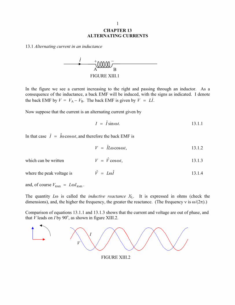
1CHAPTER 13

ALTERNATING CURRENTS 13.1 Alternating current in an inductance In the figure we see a current increasing to the right and passing through an inductor. As a consequence of the inductance, a back EMF will be induced, with the signs as indicated. I denote the back EMF by V = VA − VB. The back EMF is given by .ILV &= Now suppose that the current is an alternating current given by .sinˆ tII ω= 13.1.1 In that case ,cosˆ tII ωω=& and therefore the back EMF is ,cosˆ tLIV ωω= 13.1.2 which can be written ,cosˆ tVV ω= 13.1.3 where the peak voltage is ILV ˆˆ ω= 13.1.4 and, of course V L IRMS RMS= ω . The quantity Lω is called the inductive reactance XL. It is expressed in ohms (check the dimensions), and, the higher the frequency, the greater the reactance. (The frequency ν is ω/(2π).) Comparison of equations 13.1.1 and 13.1.3 shows that the current and voltage are out of phase, and that V leads on I by 90o, as shown in figure XIII.2.

V

I

FIGURE XIII.2

I&

A B

+ −

FIGURE XIII.1

213.2 Alternating Voltage across a Capacitor At any time, the charge Q on the capacitor is related to the potential difference V across it by Q CV= . If there is a current in the circuit, then Q is changing, and .VCI &= Now suppose that an alternating voltage given by tVV ω= sinˆ 13.2.1 is applied across the capacitor. In that case the current is ,cosˆ tVCI ωω= 13.2.2 which can be written ,cosˆ tII ω= 13.2.3 where the peak current is VCI ˆˆ ω= 13.2.4 and, of course I C VRMS RMS= ω . The quantity 1/(Cω) is called the capacitive reactance XC. It is expressed in ohms (check the dimensions), and, the higher the frequency, the smaller the reactance. (The frequency ν is ω/(2π).) Comparison of equations 13.2.1 and 13.2.3 shows that the current and voltage are out of phase, and that V lags behind I by 90o, as shown in figure XIII.4.

13.3 Complex Numbers I am now going to repeat the analyses of Sections 13.1 and 13.2 using the notation of complex numbers. In the context of alternating current theory, the imaginary unit is customarily given the symbol j rather than i, so that the symbol i is available, if need be, for electric currents. I am making the assumption that the reader is familiar with the basics of complex numbers; without that background, the reader may have difficulty with much of this chapter.

FIGURE XIII.4

I

V

FIGURE XIII.3

+ −

3 We start with the inductance. If the current is changing, there will be a back EMF given by

.ILV &= If the current is changing as ,ˆ tjeII ω= 13.3.1 then .ˆ IjejII tj ω=ω= ω& Therefore the voltage is given by V jL I= ω . 13.3.2 The quantity jLω is called the impedance of the inductor, and is j times its reactance. Equation 13.3.2 (in particular the operator j on the right hand side) tells us that V leads on I by 90o. Now suppose that an alternating voltage is applied across a capacitor. The charge on the capacitor at any time is Q = CV, and the current is .VCI &= If the voltage is changing as ,ˆ tjeVV ω= 13.3.3 then .ˆ VjejVV tj ω=ω= ω& Therefore the current is given by I jC V= ω . 13.3.4

That is to say V jC

I= −ω

. 13.3.5 The quantity − j C/ ( )ω is called the impedance of the capacitor, and is −j times its reactance. Equation 13.3.5 (in particular the operator −j on the right hand side) tells us that V lags behind I by 90o. In summary: Inductor: Reactance = Lω. Impedance = jLω. V leads on I. Capacitor: Reactance = 1/(Cω). Impedance = −j/(Cω). V lags behind I. It may be that at this stage you haven't got a very clear idea of the distinction between reactance (symbol X) and impedance (symbol Z) other than that one seems to be j or −j times the other. The next section deals with a slightly more complicated situation, namely a resistor and an inductor in series. (In practice, it may be one piece of equipment, such as a solenoid, that has both resistance and inductance.) Paradoxically, you may find it easier to understand the distinction between impedance and reactance from this more complicated situation.

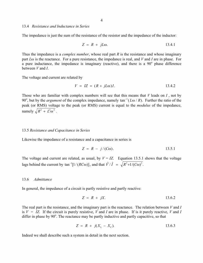
413.4 Resistance and Inductance in Series The impedance is just the sum of the resistance of the resistor and the impedance of the inductor: Z R jL= + ω. 13.4.1 Thus the impedance is a complex number, whose real part R is the resistance and whose imaginary part Lω is the reactance. For a pure resistance, the impedance is real, and V and I are in phase. For a pure inductance, the impedance is imaginary (reactive), and there is a 90o phase difference between V and I. The voltage and current are related by V IZ R jL I= = +( ) .ω 13.4.2 Those who are familiar with complex numbers will see that this means that V leads on I , not by 90o, but by the argument of the complex impedance, namely tan ( / ).−1 L Rω Further the ratio of the peak (or RMS) voltage to the peak (or RMS) current is equal to the modulus of the impedance, namely R L2 2 2+ ω . 13.5 Resistance and Capacitance in Series Likewise the impedance of a resistance and a capacitance in series is Z R j C= − / ( ) .ω 13.5.1 The voltage and current are related, as usual, by V = IZ. Equation 13.5.1 shows that the voltage lags behind the current by tan [ / ( )],−1 1 RCω and that .)/(1ˆ/ˆ 22 ω+= CRIV 13.6 Admittance In general, the impedance of a circuit is partly resistive and partly reactive: Z R jX= + . 13.6.2 The real part is the resistance, and the imaginary part is the reactance. The relation between V and I is V = IZ. If the circuit is purely resistive, V and I are in phase. If is it purely reactive, V and I differ in phase by 90o. The reactance may be partly inductive and partly capacitive, so that Z R j X X= + −( ).L C 13.6.3 Indeed we shall describe such a system in detail in the next section.

5 The reciprocal of the impedance Z is the admittance, Y.

Thus YZ R jX

= =+

1 1 . 13.6.4

And of course, since V = IZ, I = VY. Whenever we see a complex (or a purely imaginary) number in the denominator of an expression, we always immediately multiply top and bottom by the complex conjugate, so equation 13.6.4 becomes

.||*

222 XRjXR

ZZY

+−

== 13.6.5

This can be written Y G jB= + , 13.6.6 where the real part, G, is the conductance:

G RR X

=+2 2

, 13.6.7

and the imaginary part, B, is the susceptance:

B XR X

= −+2 2

. 13.6.8

The SI unit for admittance, conductance and susceptance is the siemens (or the "mho" in informal talk). I leave it to the reader to show that

R GG B

=+2 2 13.6.9

and X BG B

= −+2 2

. 13.6.10

13.7 The RLC Series Acceptor Circuit A resistance, inductance and a capacitance in series is called an "acceptor" circuit, presumably because, for some combination of the parameters, the magnitude of the inductance is a minimum,

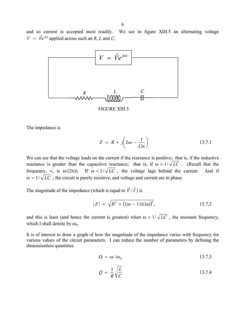
6and so current is accepted most readily. We see in figure XIII.5 an alternating voltage

tjeVV ω= ˆ applied across such an R, L and C. The impedance is

.1

ω−ω+=

CLjRZ 13.7.1

We can see that the voltage leads on the current if the reactance is positive; that is, if the inductive reactance is greater than the capacitive reactance; that is, if ω > 1/ .LC (Recall that the frequency, ν, is ω/(2π)). If ω < 1/ ,LC the voltage lags behind the current. And if ω = 1/ ,LC the circuit is purely resistive, and voltage and current are in phase. The magnitude of the impedance (which is equal to IV ˆ/ˆ ) is

( ) ,)/(1|| 22 ω−ω+= CLRZ 13.7.2 and this is least (and hence the current is greatest) when ω = 1/ ,LC the resonant frequency, which I shall denote by ω0. It is of interest to draw a graph of how the magnitude of the impedance varies with frequency for various values of the circuit parameters. I can reduce the number of parameters by defining the dimensionless quantities Ω = ω ω/ 0 13.7.3

QR

LC

=1 13.7.4

tjeVV ω= ˆ

FIGURE XIII.5

C L R

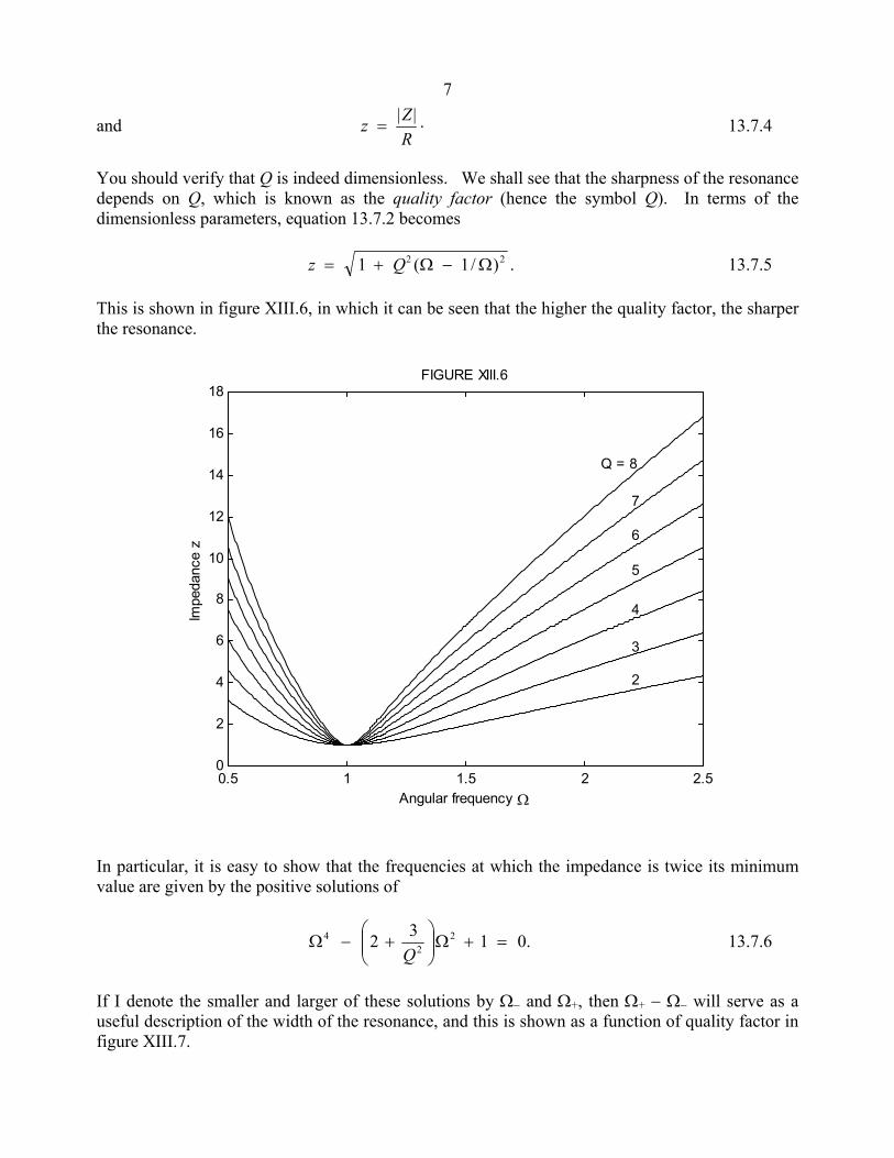
7

and z ZR

=| | . 13.7.4

You should verify that Q is indeed dimensionless. We shall see that the sharpness of the resonance depends on Q, which is known as the quality factor (hence the symbol Q). In terms of the dimensionless parameters, equation 13.7.2 becomes z Q= + −1 12 2( / ) .Ω Ω 13.7.5 This is shown in figure XIII.6, in which it can be seen that the higher the quality factor, the sharper the resonance.

0.5 1 1.5 2 2.50

2

4

6

8

10

12

14

16

18

Angular frequency Ω

Impe

danc

e z

FIGURE XIII.6

Q = 8

7

6

5

4

3

2

In particular, it is easy to show that the frequencies at which the impedance is twice its minimum value are given by the positive solutions of

.0132 22

4 =+Ω

+−Ω

Q 13.7.6

If I denote the smaller and larger of these solutions by Ω− and Ω+, then Ω+ − Ω− will serve as a useful description of the width of the resonance, and this is shown as a function of quality factor in figure XIII.7.

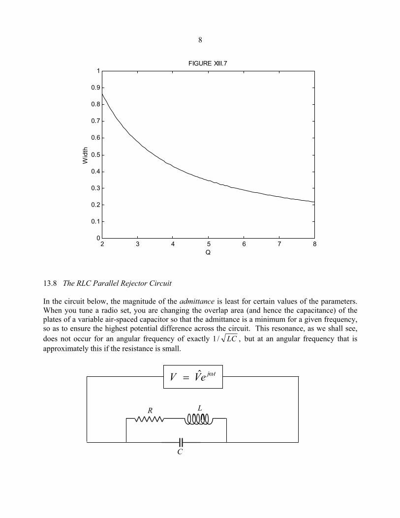
8

2 3 4 5 6 7 80

0.1

0.2

0.3

0.4

0.5

0.6

0.7

0.8

0.9

1

Q

Wid

th

FIGURE XIII.7

13.8 The RLC Parallel Rejector Circuit In the circuit below, the magnitude of the admittance is least for certain values of the parameters. When you tune a radio set, you are changing the overlap area (and hence the capacitance) of the plates of a variable air-spaced capacitor so that the admittance is a minimum for a given frequency, so as to ensure the highest potential difference across the circuit. This resonance, as we shall see, does not occur for an angular frequency of exactly 1/ ,LC but at an angular frequency that is approximately this if the resistance is small.

tjeVV ω= ˆ

C

L R

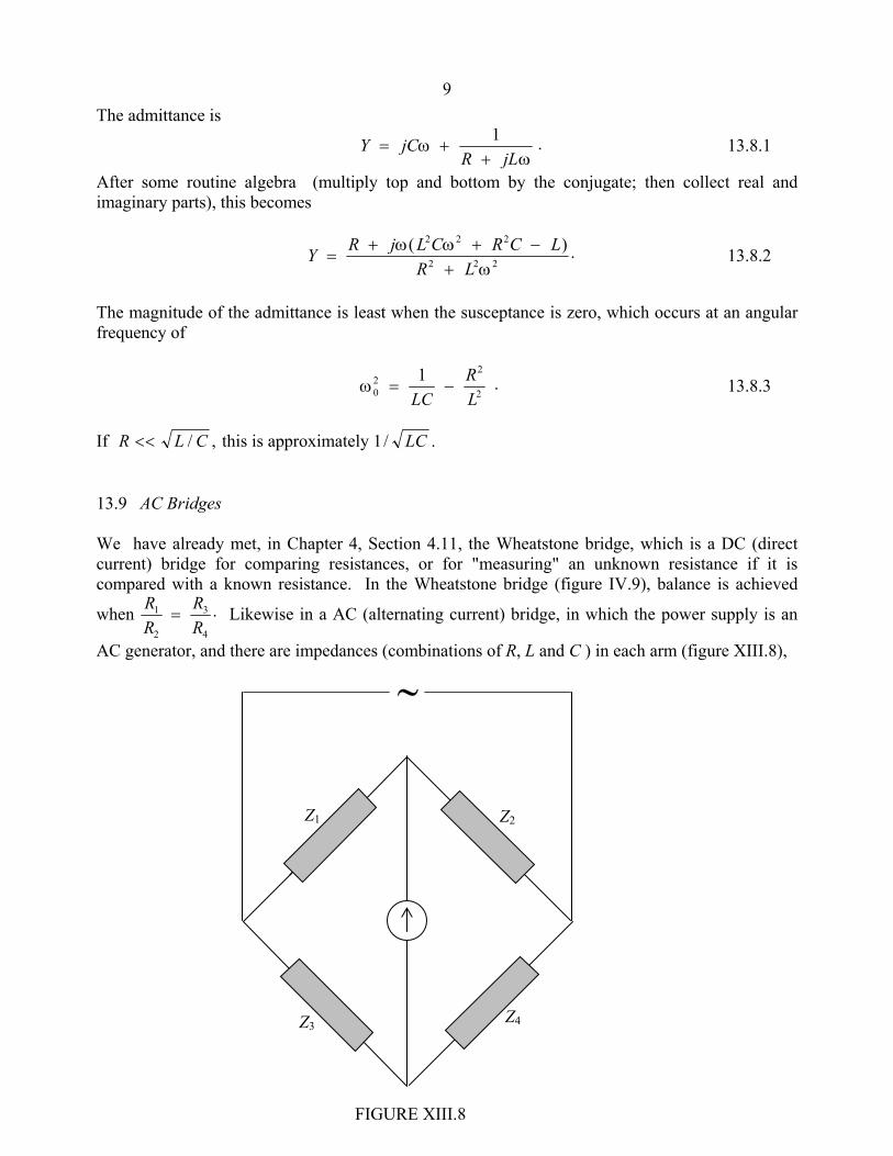
9The admittance is

Y jCR jL

= ++

ωω

1 . 13.8.1

After some routine algebra (multiply top and bottom by the conjugate; then collect real and imaginary parts), this becomes

Y R j L C R C LR L

=+ + −

+ω ω

ω( ) .

2 2 2

2 2 2 13.8.2

The magnitude of the admittance is least when the susceptance is zero, which occurs at an angular frequency of

ω02

2

2

1= −

LCRL

. 13.8.3

If R L C<< / , this is approximately 1/ .LC 13.9 AC Bridges We have already met, in Chapter 4, Section 4.11, the Wheatstone bridge, which is a DC (direct current) bridge for comparing resistances, or for "measuring" an unknown resistance if it is compared with a known resistance. In the Wheatstone bridge (figure IV.9), balance is achieved

when RR

RR

1

2

3

4

= . Likewise in a AC (alternating current) bridge, in which the power supply is an

AC generator, and there are impedances (combinations of R, L and C ) in each arm (figure XIII.8),

Z1 Z2

Z3 Z4

FIGURE XIII.8

i

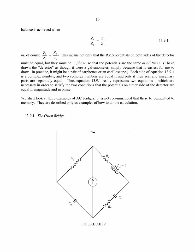
10 balance is achieved when

ZZ

ZZ

1

2

3

4

= 13.9.1

or, of course, ZZ

ZZ

1

3

2

4

= . This means not only that the RMS potentials on both sides of the detector

must be equal, but they must be in phase, so that the potentials are the same at all times. (I have drawn the "detector" as though it were a galvanometer, simply because that is easiest for me to draw. In practice, it might be a pair of earphones or an oscilloscope.) Each side of equation 13.9.1 is a complex number, and two complex numbers are equal if and only if their real and imaginary parts are separately equal. Thus equation 13.9.1 really represents two equations – which are necessary in order to satisfy the two conditions that the potentials on either side of the detector are equal in magnitude and in phase. We shall look at three examples of AC bridges. It is not recommended that these be committed to memory. They are described only as examples of how to do the calculation. 13 9.1 The Owen Bridge

i

R1 R2

R4

FIGURE XIII.9

L2 = ?

C4

C3

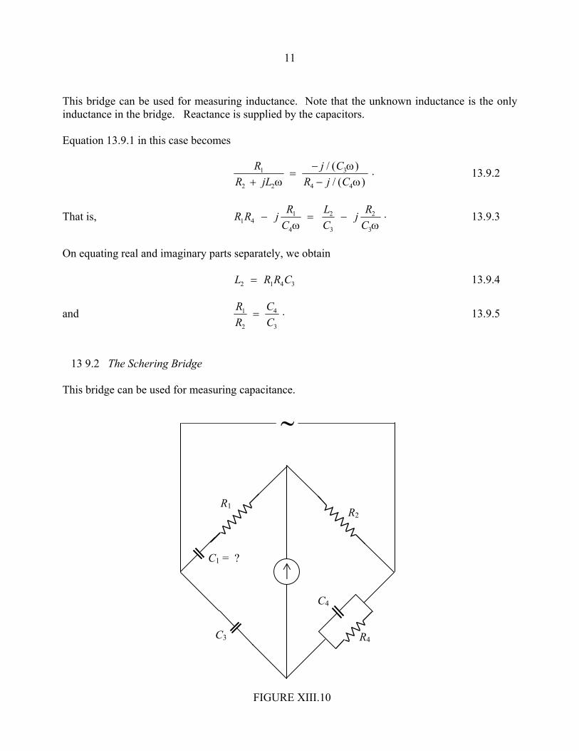
11

This bridge can be used for measuring inductance. Note that the unknown inductance is the only inductance in the bridge. Reactance is supplied by the capacitors. Equation 13.9.1 in this case becomes

RR jL

j CR j C

1

2 2

3

4 4+=

−−ω

ωω

/ ( )/ ( )

. 13.9.2

That is, R R j RC

LC

j RC1 4

1

4

2

3

2

3

− = −ω ω

. 13.9.3

On equating real and imaginary parts separately, we obtain L R R C2 1 4 3= 13.9.4

and RR

CC

1

2

4

3

= . 13.9.5

13 9.2 The Schering Bridge This bridge can be used for measuring capacitance.

i

R1 R2

R4

FIGURE XIII.10

C4

C3

C1 = ?

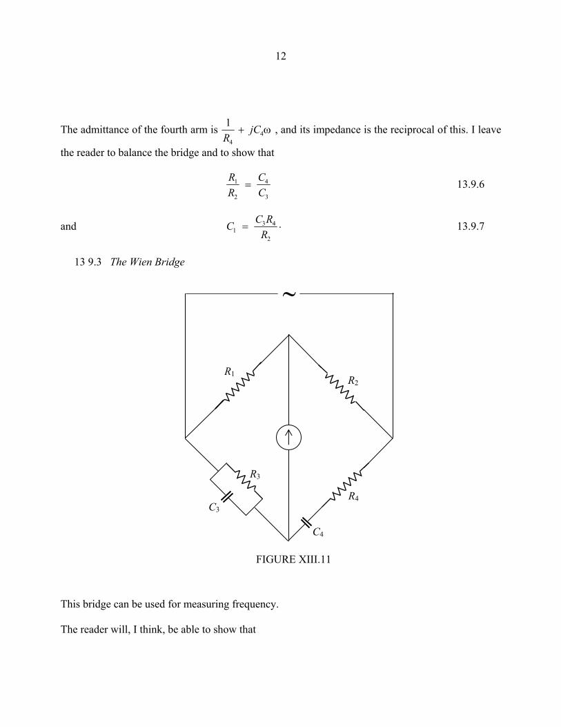
12

The admittance of the fourth arm is 1

44R

jC+ ω , and its impedance is the reciprocal of this. I leave

the reader to balance the bridge and to show that

RR

CC

1

2

4

3

= 13.9.6

and C C RR13 4

2

= . 13.9.7

13 9.3 The Wien Bridge This bridge can be used for measuring frequency. The reader will, I think, be able to show that

i

R1 R2

R3

FIGURE XIII.11

C4

C3

R4

13

RR

CC

RR

4

3

3

4

2

1

+ = 13.9.8

and ω2

3 4 3 4

1=

R R C C. 13.9.10

13.10 The Transformer We met the transformer briefly in Section 10.9. There we pointed out that the EMF induced in the secondary coil is equal to the number of turns in the secondary coil times the rate of change of magnetic flux; and the flux is proportional to the EMF applied to the primary times the number of turns in the primary. Hence we deduced the well known relation

VV

NN

2

1

2

1

= 13.10.1

relating the primary and secondary voltages to the number of turns in each. We now look at the transformer in more detail; in particular, we look at what happens when we connect the secondary coil to a circuit and take power from it. In figure XIII.12, we apply an AC EMF tjeVV ω= ˆ to the primary circuit. The self inductance of the primary coil is Ll, and an alternating current I1 flows in the primary circuit. The self inductance of the secondary coil is L2, and the mutual inductance of the two coils is M. If the coupling between the two coils is very tight, then M L L= 1 2 ; otherwise it is less than this. I am supposing that the resistance of the primary circuit is much smaller than the reactance, so I am going to neglect it.

i

FIGURE XIII.12

tjeVV ω= ˆ

I1 I2

L2 L1

M

R

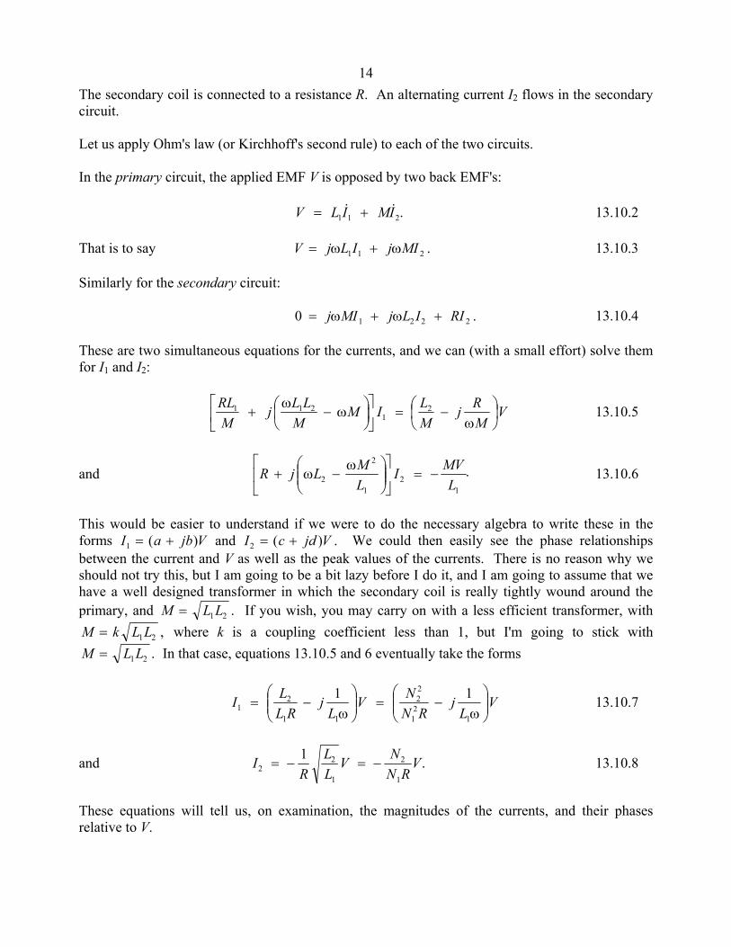
14The secondary coil is connected to a resistance R. An alternating current I2 flows in the secondary circuit. Let us apply Ohm's law (or Kirchhoff's second rule) to each of the two circuits. In the primary circuit, the applied EMF V is opposed by two back EMF's: .211 IMILV && += 13.10.2 That is to say V j L I j MI= +ω ω1 1 2 . 13.10.3 Similarly for the secondary circuit: 0 1 2 2 2= + +j MI j L I RIω ω . 13.10.4 These are two simultaneous equations for the currents, and we can (with a small effort) solve them for I1 and I2:

VMRj

MLIM

MLLj

MRL

ω−=

ω−

ω+ 2

1211 13.10.5

and .1

21

2

2 LMVI

LMLjR −=

ω−ω+ 13.10.6

This would be easier to understand if we were to do the necessary algebra to write these in the forms I a jb V I c jd V1 2= + = +( ) ( ) .and We could then easily see the phase relationships between the current and V as well as the peak values of the currents. There is no reason why we should not try this, but I am going to be a bit lazy before I do it, and I am going to assume that we have a well designed transformer in which the secondary coil is really tightly wound around the primary, and M L L= 1 2 . If you wish, you may carry on with a less efficient transformer, with M k L L= 1 2 , where k is a coupling coefficient less than 1, but I'm going to stick with M L L= 1 2 . In that case, equations 13.10.5 and 6 eventually take the forms

VL

jRN

NVL

jRL

LI

ω

−=

ω

−=1

21

22

11

21

11 13.10.7

and IR

LL

V NN R

V22

1

2

1

1= − = − . 13.10.8

These equations will tell us, on examination, the magnitudes of the currents, and their phases relative to V.

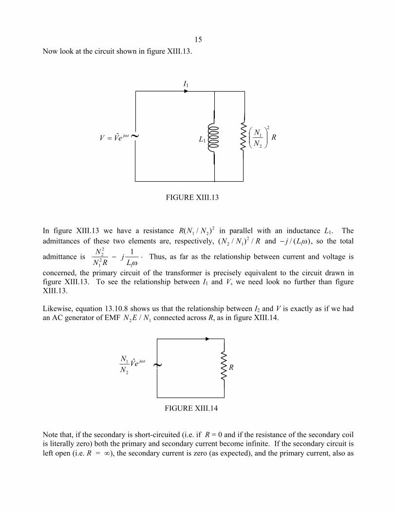
15Now look at the circuit shown in figure XIII.13. In figure XIII.13 we have a resistance R N N( / )1 2

2 in parallel with an inductance L1. The admittances of these two elements are, respectively, ( / ) /N N R2 1

2 and − j L/ ( )1ω , so the total

admittance is NN R

jL

22

12

1

1−

ω. Thus, as far as the relationship between current and voltage is

concerned, the primary circuit of the transformer is precisely equivalent to the circuit drawn in figure XIII.13. To see the relationship between I1 and V, we need look no further than figure XIII.13. Likewise, equation 13.10.8 shows us that the relationship between I2 and V is exactly as if we had an AC generator of EMF N E N2 1/ connected across R, as in figure XIII.14. Note that, if the secondary is short-circuited (i.e. if R = 0 and if the resistance of the secondary coil is literally zero) both the primary and secondary current become infinite. If the secondary circuit is left open (i.e. R = ∞), the secondary current is zero (as expected), and the primary current, also as

i

FIGURE XIII.13

tjeVV ω= ˆ

I1

L1 RNN

2

2

1

tjeVNN ωˆ

2

1 i

FIGURE XIII.14

R

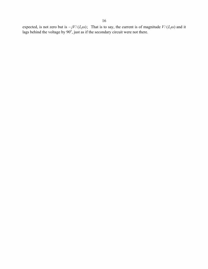
16expected, is not zero but is − jV L/ ( ) ;1ω That is to say, the current is of magnitude V L/ ( )1ω and it lags behind the voltage by 90o, just as if the secondary circuit were not there.

1CHAPTER 14

LAPLACE TRANSFORMS

14.1 Introduction If y(x) is a function of x, where x lies in the range 0 to ∞, then the function y p( ), defined by

dxxyepy px )()(0∫∞ −= , 14.1.1

is called the Laplace transform of y(x). However, in this chapter, where we shall be applying Laplace transforms to electrical circuits, y will most often be a voltage or current that is varying with time rather than with "x". Thus I shall use t as our variable rather than x, and I shall use s rather than p (although it will be noted that, as yet, I have given no particular physical meaning to either p or to s.) Thus I shall define the Laplace transform with the notation

,)()(0

dttyesy st∫∞ −= 14.1.2

it being understood that t lies in the range 0 to ∞. For short, I could write this as y s y t( ) ( ) .= L 14.1.3 When we first learned differential calculus, we soon learned that there were just a few functions whose derivatives it was worth committing to memory. Thus we learned the derivatives ofx x en x, sin , and a very few more. We found that we could readily find the derivatives of more complicated functions by means of a few simple rules, such as how to differentiate a product of two functions, or a function of a function, and so on. Likewise, we have to know only a very few basic Laplace transforms; there are a few simple rules that will enable us to calculate more complicated ones. After we had learned differential calculus, we came across integral calculus. This was the inverse process from differentiation. We had to ask: What function would we have had to differentiate in order to arrive at this function? It was as though we were given the answer to a problem, and had to deduce what the question was. It will be a similar situation with Laplace transforms. We shall often be given a function y s( ), and we shall want to know: what function y(t) is this the Laplace transform of? In other words, we shall need to know the inverse Laplace transform: y t y s( ) ( ).= −L 1 14.1.4 We shall find that facility in calculating Laplace transforms and their inverses leads to very quick ways of solving some types of differential equations – in particular the types of differential equations that arise in electrical theory. We can use Laplace transforms to see the relations between varying current and voltages in circuits containing resistance, capacitance and inductance.

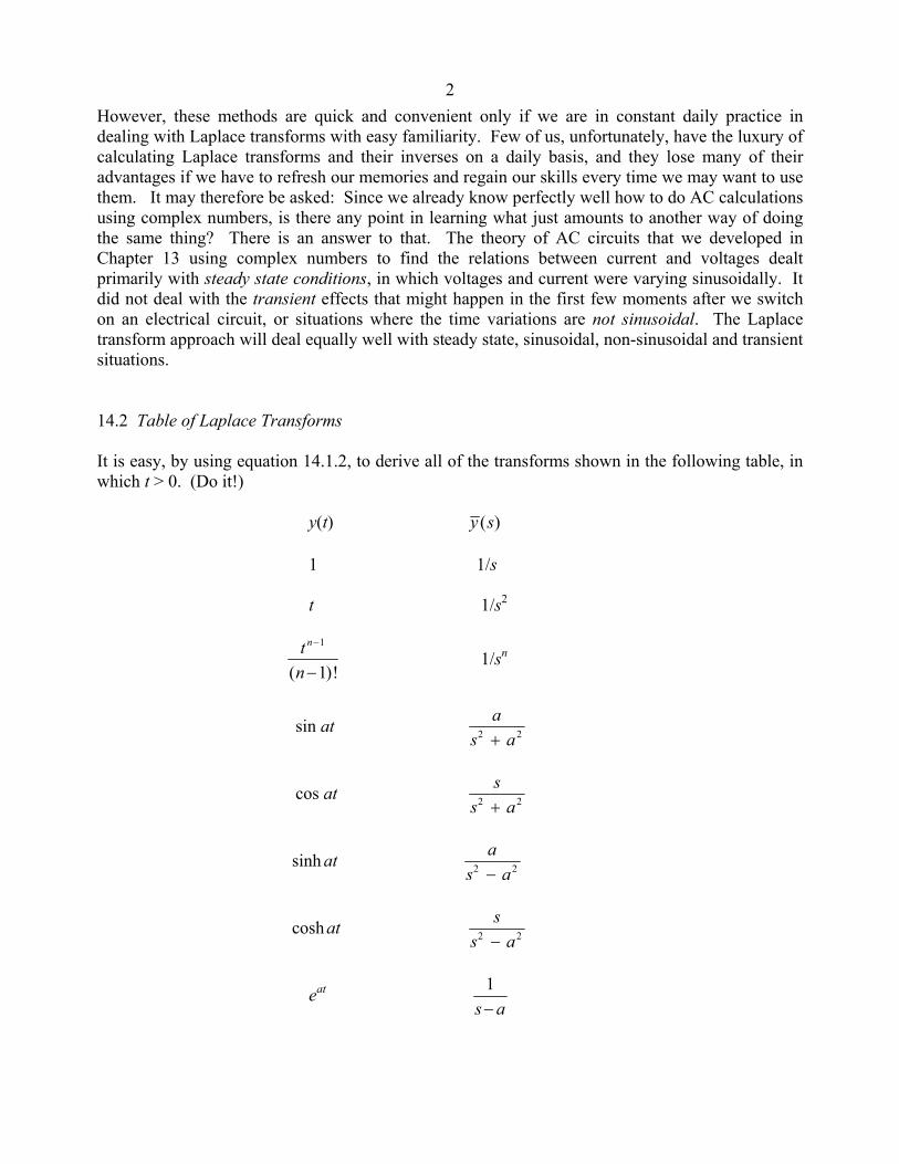
2However, these methods are quick and convenient only if we are in constant daily practice in dealing with Laplace transforms with easy familiarity. Few of us, unfortunately, have the luxury of calculating Laplace transforms and their inverses on a daily basis, and they lose many of their advantages if we have to refresh our memories and regain our skills every time we may want to use them. It may therefore be asked: Since we already know perfectly well how to do AC calculations using complex numbers, is there any point in learning what just amounts to another way of doing the same thing? There is an answer to that. The theory of AC circuits that we developed in Chapter 13 using complex numbers to find the relations between current and voltages dealt primarily with steady state conditions, in which voltages and current were varying sinusoidally. It did not deal with the transient effects that might happen in the first few moments after we switch on an electrical circuit, or situations where the time variations are not sinusoidal. The Laplace transform approach will deal equally well with steady state, sinusoidal, non-sinusoidal and transient situations. 14.2 Table of Laplace Transforms It is easy, by using equation 14.1.2, to derive all of the transforms shown in the following table, in which t > 0. (Do it!) y(t) y s( )

1 1/s

t 1/s2

tn

n −

−

1

1( )! 1/sn

sin at as a2 2+

cos at ss a2 2+

sinh at a

s a2 2−

cosh at ss a2 2−

eat 1s a−

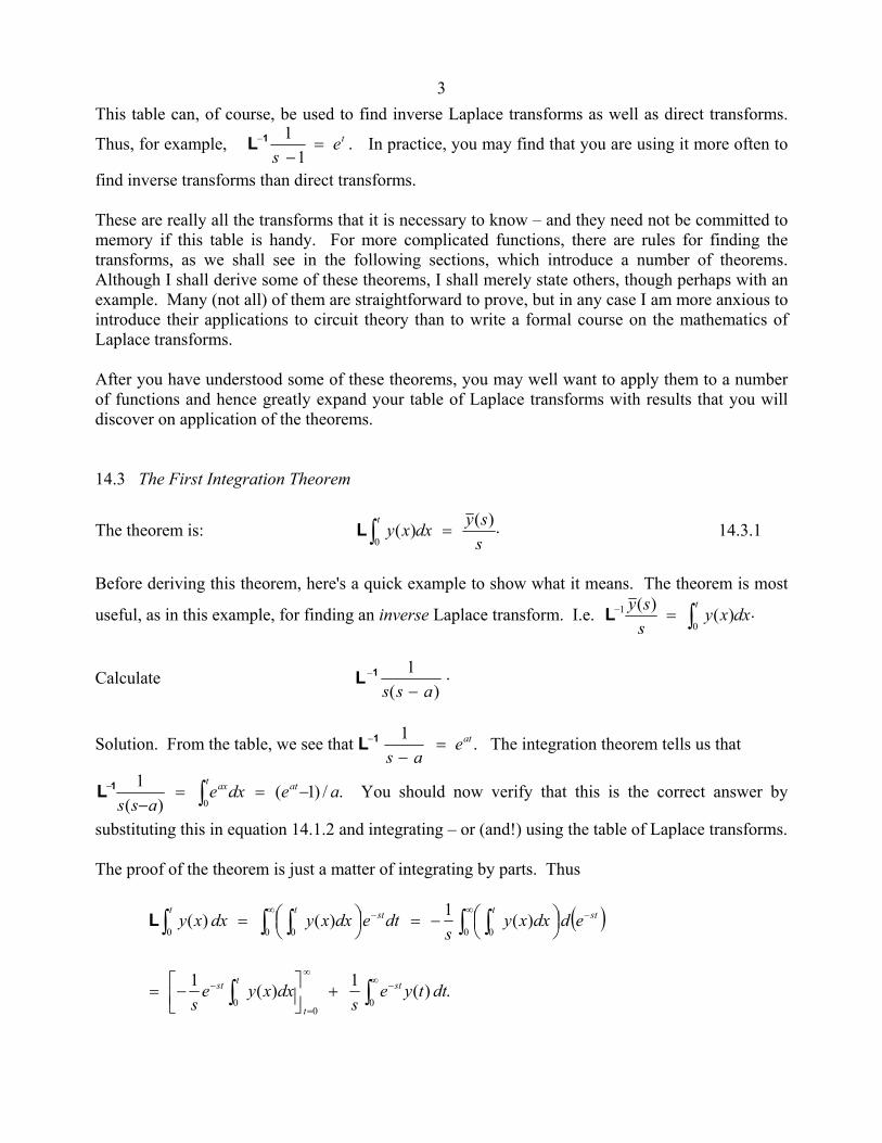
3This table can, of course, be used to find inverse Laplace transforms as well as direct transforms.

Thus, for example, L 1−

−=

11s

et . In practice, you may find that you are using it more often to

find inverse transforms than direct transforms. These are really all the transforms that it is necessary to know – and they need not be committed to memory if this table is handy. For more complicated functions, there are rules for finding the transforms, as we shall see in the following sections, which introduce a number of theorems. Although I shall derive some of these theorems, I shall merely state others, though perhaps with an example. Many (not all) of them are straightforward to prove, but in any case I am more anxious to introduce their applications to circuit theory than to write a formal course on the mathematics of Laplace transforms. After you have understood some of these theorems, you may well want to apply them to a number of functions and hence greatly expand your table of Laplace transforms with results that you will discover on application of the theorems. 14.3 The First Integration Theorem

The theorem is: .)()(0 s

sydxxyt

=∫L 14.3.1

Before deriving this theorem, here's a quick example to show what it means. The theorem is most

useful, as in this example, for finding an inverse Laplace transform. I.e. .)()(0

1 ∫=− tdxxy

ssyL

Calculate L 1−

−1

s s a( ).

Solution. From the table, we see that L 1−

−=

1s a

eat . The integration theorem tells us that

./)1()(

10

aedxeass

att ax −==− ∫−1L You should now verify that this is the correct answer by

substituting this in equation 14.1.2 and integrating – or (and!) using the table of Laplace transforms. The proof of the theorem is just a matter of integrating by parts. Thus

( )sttsttteddxxy

sdtedxxydxxy −∞−∞

∫ ∫∫ ∫∫

−=

=

0 00 00)(1)()(L

.)(1)(10

00

dttyes

dxxyes

st

t

tst ∫∫∞ −

∞

=

− +

−=

4

The expression in brackets is zero at both limits, and therefore the theorem is proved. 14.4 The Second Integration Theorem (Dividing a Function by t) This theorem looks very like the first integration theorem, but "the other way round". It is

.)()( dxxytty

s∫∞

=

L 14.4.1

I'll leave it for the reader to derive the theorem. Here I just give an example of its use. Whereas the first integration theorem is most useful in finding inverse transforms, the second integration theorem is more useful for finding direct transforms.

Example: Calculate .sin

tatL

This means calculate .sin0

dtt

ate st

∫∞ −

While this integral can no doubt be done, you may find it a bit daunting, and the second integration theorem provides an alternative way of doing it, resulting in an easier integral. Note that the right hand side of equation 14.4.1 is a function of s, not of x, which is just a dummy variable. The function y x( ) is the Laplace transform, with x as argument, of y(t). In our particular

case, y(t) is sin at, so that, from the table, y x aa x

( ) .=+2 2 The second integration theorem , then,

tells us that .sin22 dx

xaa

tat

s∫∞

+=

L This is a much easier integral. It is

.tantan2

tan 111

=

−

π=

−−

∞−

sa

as

ax

s

You may want to add this result to your table of

Laplace integrals. Indeed, you may already want to expand the table considerably by applying both integration theorems to several functions. 14.5 Shifting Theorem This is a very useful theorem, and one that is almost trivial to prove. (Try it!) It is ( ) .)()( asytye at +=−L 14.5.1 For example, from the table, we have L( ) / .t s= 1 2 The shifting theorem tells us that

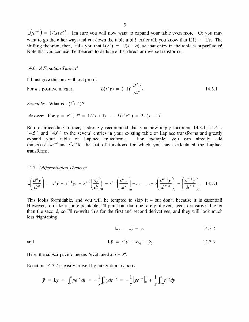
5

( ) .)/(1 2aste at +=−L I'm sure you will now want to expand your table even more. Or you may want to go the other way, and cut down the table a bit! After all, you know that L(1) = 1/s. The shifting theorem, then, tells you that L(eat) = 1/(s − a), so that entry in the table is superfluous! Note that you can use the theorem to deduce either direct or inverse transforms. 14.6 A Function Times tn I'll just give this one with out proof:

For n a positive integer, L t y d yds

n nn( ) ( ) .= −1

2

14.6.1

Example: What is L( ) ?t e t2 − Answer: For y e y s L t e st t= = + ∴ = +− −, / ( ) . ( ) / ( ) .1 1 2 12 3 Before proceeding further, I strongly recommend that you now apply theorems 14.3.1, 14.4.1, 14.5.1 and 14.6.1 to the several entries in your existing table of Laplace transforms and greatly expand your table of Laplace transforms. For example, you can already add (sin ) / ,at t te t eat t− −and 2 to the list of functions for which you have calculated the Laplace transforms. 14.7 Differentiation Theorem

.0

1

1

02

2

02

23

0

20

1

−

−−

−

−−=

−

−

−

−−−−

n

n

n

nnnnn

n

n

dtyd

dtyds

dtyds

dtdysysys

dtyd

KKL 14.7.1

This looks formidable, and you will be tempted to skip it – but don't, because it is essential! However, to make it more palatable, I'll point out that one rarely, if ever, needs derivatives higher than the second, so I'll re-write this for the first and second derivatives, and they will look much less frightening. 0yysy −=&L 14.7.2 and .00

2 ysyysy &&& −−=L 14.7.3 Here, the subscript zero means "evaluated at t = 0". Equation 14.7.2 is easily proved by integration by parts:

[ ] dyes

yes

ydes

dtyeyyt

stststst ∫∫∫∞

=

−∞−∞ −∞ − +−=−===0000

111L

6

.111100 y

sy

sdty

sy

s&& L+=+= ∫ 14.7.4

∴ .0yysyL −=& 14.7.5 From this, .)( 00

20000 ysyysyyyssyysLyysyL &&&&&&&& −−=−−=−=−= 14.7.6

Apply this over and over again, and you arrive at equation 14.7.1 14.8 A First Order Differential Equation Solve ,32 tteyy =+& with initial condition y0 = 0. If you are in good practice with solving this type of equation, you will probably multiply it through by e2t, so that it becomes

( ) ,3 32 tt teyedtd

=

from which y t e Cet t= − + −( ) .1

32

(You can now substitute this back into the original differential equation, to verify that it is indeed the correct solution.) With the given initial condition, it is quickly found that C = 1

3, so that the solution is

y te e et t t= − + −1

313

2 . Now, here's the same solution, using Laplace transforms. We take the Laplace transform of both sides of the original differential equation:

sy y tes

t+ = =−

2 3 31 2L( )

( ).

Thus ys s

=+ −

32 1 2( )( )

.

Partial fractions: .)1(

11

131

21

31

2−+

−

−

+

=sss

y

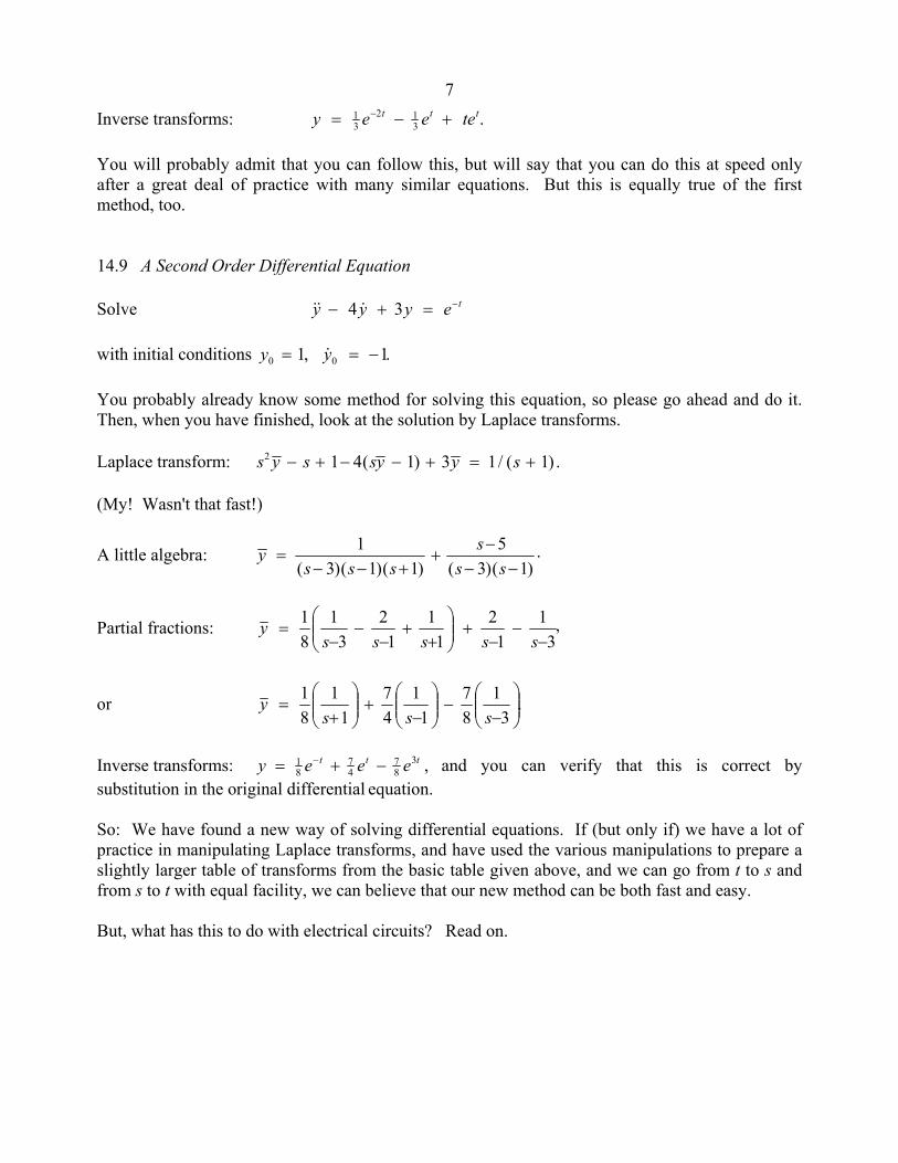
7

Inverse transforms: .312

31 ttt teeey +−= −

You will probably admit that you can follow this, but will say that you can do this at speed only after a great deal of practice with many similar equations. But this is equally true of the first method, too. 14.9 A Second Order Differential Equation Solve teyyy −=+− 34 &&& with initial conditions .1,1 00 −== yy & You probably already know some method for solving this equation, so please go ahead and do it. Then, when you have finished, look at the solution by Laplace transforms. Laplace transform: s y s sy y s2 1 4 1 3 1 1− + − − + = +( ) / ( ) . (My! Wasn't that fast!)

A little algebra: ys s s

ss s

=− − +

+−

− −1

3 1 15

3 1( )( )( ) ( )( ).

Partial fractions: ,3

11

21

11

23

181

−−

−+

+

+−

−−

=sssss

y

or .3

187

11

47

11

81

−

−

−

+

+

=sss

y

Inverse transforms: y e e et t t= + −−1

874

78

3 , and you can verify that this is correct by substitution in the original differential equation. So: We have found a new way of solving differential equations. If (but only if) we have a lot of practice in manipulating Laplace transforms, and have used the various manipulations to prepare a slightly larger table of transforms from the basic table given above, and we can go from t to s and from s to t with equal facility, we can believe that our new method can be both fast and easy. But, what has this to do with electrical circuits? Read on.

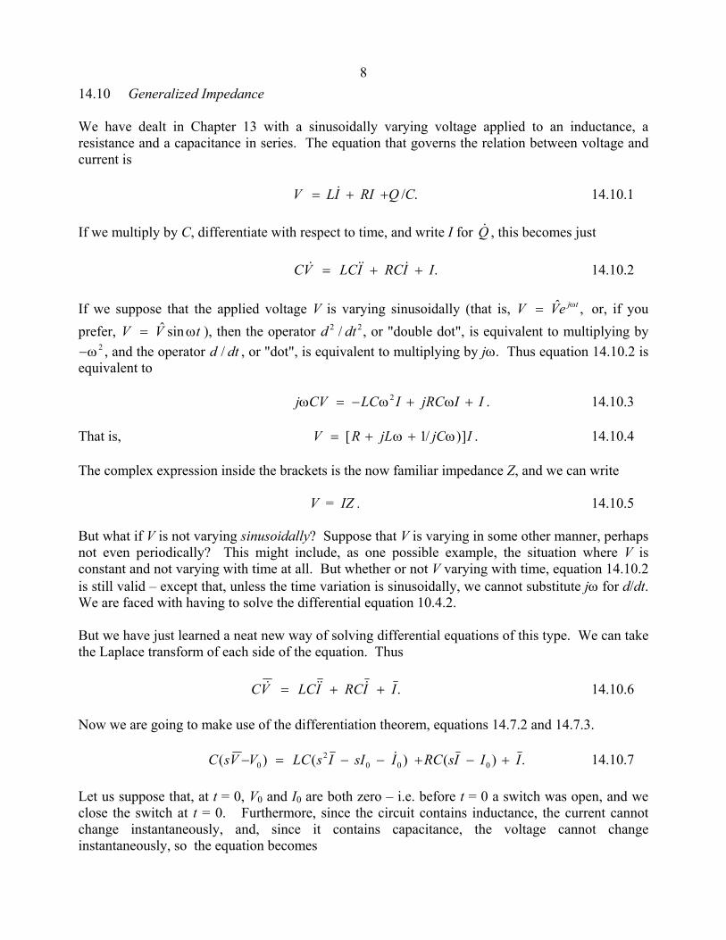
814.10 Generalized Impedance We have dealt in Chapter 13 with a sinusoidally varying voltage applied to an inductance, a resistance and a capacitance in series. The equation that governs the relation between voltage and current is ./CQRIILV ++= & 14.10.1 If we multiply by C, differentiate with respect to time, and write I for Q& , this becomes just .IIRCILCVC ++= &&&& 14.10.2 If we suppose that the applied voltage V is varying sinusoidally (that is, ,ˆ tjeVV ω= or, if you prefer, tVV ω= sinˆ ), then the operator d dt2 2/ , or "double dot", is equivalent to multiplying by −ω2 , and the operator d dt/ , or "dot", is equivalent to multiplying by jω. Thus equation 14.10.2 is equivalent to j CV LC I jRC I Iω ω ω= − + +2 . 14.10.3 That is, V R jL jC I= + +[ / )] .ω ω1 14.10.4 The complex expression inside the brackets is the now familiar impedance Z, and we can write V = IZ . 14.10.5 But what if V is not varying sinusoidally? Suppose that V is varying in some other manner, perhaps not even periodically? This might include, as one possible example, the situation where V is constant and not varying with time at all. But whether or not V varying with time, equation 14.10.2 is still valid – except that, unless the time variation is sinusoidally, we cannot substitute jω for d/dt. We are faced with having to solve the differential equation 10.4.2. But we have just learned a neat new way of solving differential equations of this type. We can take the Laplace transform of each side of the equation. Thus .IIRCILCVC ++= &&&& 14.10.6 Now we are going to make use of the differentiation theorem, equations 14.7.2 and 14.7.3. .)()()( 000

20 IIIsRCIsIIsLCVVsC +−+−−=− & 14.10.7

Let us suppose that, at t = 0, V0 and I0 are both zero – i.e. before t = 0 a switch was open, and we close the switch at t = 0. Furthermore, since the circuit contains inductance, the current cannot change instantaneously, and, since it contains capacitance, the voltage cannot change instantaneously, so the equation becomes

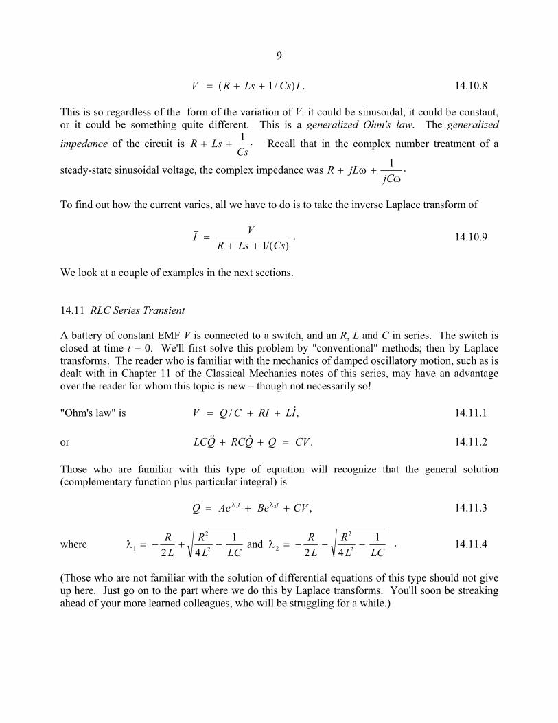
9 V R Ls Cs I= + +( / ) .1 14.10.8 This is so regardless of the form of the variation of V: it could be sinusoidal, it could be constant, or it could be something quite different. This is a generalized Ohm's law. The generalized

impedance of the circuit is R LsCs

+ +1 . Recall that in the complex number treatment of a

steady-state sinusoidal voltage, the complex impedance was R jLjC

+ +ωω

1 .

To find out how the current varies, all we have to do is to take the inverse Laplace transform of

I VR Ls Cs

=+ + 1/( )

. 14.10.9

We look at a couple of examples in the next sections. 14.11 RLC Series Transient A battery of constant EMF V is connected to a switch, and an R, L and C in series. The switch is closed at time t = 0. We'll first solve this problem by "conventional" methods; then by Laplace transforms. The reader who is familiar with the mechanics of damped oscillatory motion, such as is dealt with in Chapter 11 of the Classical Mechanics notes of this series, may have an advantage over the reader for whom this topic is new – though not necessarily so! "Ohm's law" is ,/ ILRICQV &++= 14.11.1 or .CVQQRCQLC =++ &&& 14.11.2 Those who are familiar with this type of equation will recognize that the general solution (complementary function plus particular integral) is Q Ae Be CVt t= + +λ λ1 2 , 14.11.3

where λ λ1

2

2 2

2

22 41

2 41

= − + − = − − −RL

RL LC

RL

RL LC

and . 14.11.4

(Those who are not familiar with the solution of differential equations of this type should not give up here. Just go on to the part where we do this by Laplace transforms. You'll soon be streaking ahead of your more learned colleagues, who will be struggling for a while.)

10

Case I. RL LC

2

241

− is positive. For short I'm going to write equations 14.11.4 as

λ λ1 2= − + = − −a k a kand . 14.11.5 Then Q Ae Be CVa k t a k t= + +− − − +( ) ( ) 14.11.6 and, by differentiation with respect to time, I A a k e B a k ea k t a k t= − − − +− − − +( ) ( ) .( ) ( ) 14.11.7 At t = 0, Q and I are both zero, from which we find that

A a k CVk

B a k CVk

= −+

=−( ) ( ) .

2 2and 14.11.8

Thus CVekkae

kkaQ tkatka

+

−

+

+

−= +−−− 122

)()( 14.11.9

and ( ) .2

)()(22

CVeekkaI tkatka

−

−= +−−− 14.11.10

On recalling the meanings of a and k and the sinh function, and a little algebra, we obtain

I VLk

e ktat= − sinh . 14.11.11

Exercise: Verify that this equation is dimensionally correct. Draw a graph of I : t. The current is, of course, zero at t = 0 and ∞. What is the maximum current, and when does it occur?

Case II. RL LC

2

241

− is zero. In this case, those who are in practice with differential equations

will obtain for the general solution Q e A Bt CVt= + +λ ( ) , 14.11.12 where λ = − R L/ ( ) ,2 14.11.13 from which I A Bt e Bet t= + +λ λ λ( ) . 14.11.14 After applying the initial conditions that Q and I are initially zero, we obtain

11

−−= − )2/(

211 LtRe

LRtCVQ 14.11.15

and I VL

te Rt L= − /( ) .2 14.11.16

As in case II, this starts and ends at zero and goes through a maximum, and you may wish to calculate what the maximum current is and when it occurs.

Case III. RL LC

2

241

− is negative. In this case, I am going to write equations 14.11.4 as

λ ω λ ω1 2= − + = − −a j a jand , 14.11.17

where a RL LC

RL

= = −2

14

22

2and ω . 14.11.18

All that is necessary, then, is to repeat the analysis for Case I, but to substitute −ω2 for k2 and jω for k, and, provided that you know that sinh sin ,j t j tω ω= you finish with

I VL

e tat= −

ωωsin . 14.11.19

This is lightly damped oscillatory motion. Now let us try the same problem using Laplace transforms. Recall that we have a V in series with an R , L and C, and that initially IIQ &and, are all zero. (The circuit contains capacitance, so Q cannot change instantaneously; it contains inductance, so I cannot change instantaneously.) Immediately, automatically and with scarcely a thought, our first line is the generalized Ohm's law, with the Laplace transforms of V and I and the generalized impedance: [ ] .)/(1 ICsLsRV ++= 14.11.20 Since V is constant, reference to the very first entry in your table of transforms shows that V V s= / , and so

[ ] ,)()/(1 2 cbssL

VCsLsRs

VI++

=++

= 14.11.21

where b R L c LC= =/ / ( ) .and 1 14.11.22

12Case I. b c2 4> .

.111))((

1

β−

−α−

β−α

=

β−α−

=ssL

VssL

VI 14.11.23

Here, of course, 2 4 2 42 2α β= − + − = − − −b b c b b cand 14.11.24 On taking the inverse transforms, we find that

).()

1 tt eeLVI βα −

β−α

= 14.11.25

From there it is a matter of routine algebra (do it!) to show that this is exactly the same as equation 14.11.11. In order to arrive at this result, it wasn't at all necessary to know how to solve differential equations. All that was necessary was to understand generalized impedance and to look up a table of Laplace transforms. Case II. b c2 4= . In this case, equation 14.11.21 is of the form

I VL s

=−

.( )

,12α

14.11.26

where α = − 1

2 b . If you have dutifully expanded your original table of Laplace transforms, as suggested, you will probably already have an entry for the inverse transform of the right hand side. If not, you know that the Laplace transform of t is 1/s2, so you can just apply the shifting theorem to see that the Laplace transform of t e stα αis 1 2/ ( ) .− Thus

I VL

te t= α 14.11.27

which is the same as equation 14.11.16. [Gosh – what could be quicker and easier than that!?] Case III. b c2 4< . This time, we'll complete the square in the denominator of equation 14.11. 21:

13

I VL s b c b

VL s b

=+ + −

=+ +

.( ) ( ) ( )

,112

2 14

2 12

2 2ωω

ω 14.11.28

where I have introduced ω with obvious notation. On taking the inverse transform (from our table, with a little help from the shifting theorem) we obtain

I VL

e tbt= −

ωω. sin ,

12 14.11.29

which is the same as equation 14.11.19. With this brief introductory chapter to the application of Laplace transforms to electrical circuitry, we have just opened a door by a tiny crack to glimpse the potential great power of this method. With practice, it can be used to solve complicated problems of many sorts with great rapidity. All we have so far is a tiny glimpse. I shall end this chapter with just one more example, in the hope that this short introduction will whet the reader's appetite to learn more about this technique. 14.12 Another Example The circuit in figure XIV.1 contains two equal resistances, two equal capacitances, and a battery. The battery is connected at time t = 0. Find the charges held by the capacitors after time t. Apply Kirchhoff’s second rule to each half: ,)( 221 CVQRCQQ =++ && 14.12.1 and .0211 =−+ QQRCQ& 14.12.2 Eliminate Q2: .3 111

22 CVQRCQQCR =++&& 14.12.3 Transform, with 11 and QQ & initially zero:

+ +

R

+−

−

−

+ +−

−

R

C V

I1+ I2 I1

I2 Q1 Q2 C

FIGURE XIV.1

14

.)13( 1222

sCVQRCssCR =++ 14.12.4

I.e. ,.)3(

1221

2 Vaasss

QCR++

= 14.12.5

where )./(1 RCa = 14.12.6

That is .)382.0)(618.2(

11

2 Vasass

QCR++

= 14.12.7

Partial fractions: .382.0

1708.1618.2

1708.0121

2

aV

asassQCR

+

−+

+= 14.12.8

That is, .382.0

1708.1618.2

1708.011 CV

asassQ

+

−+

+= 14.12.8

Inverse transform: [ ].1708.11708.01 )/(382.0)/(618.2

1RCtRCt eeQ −− −+= 14.12.9

The current can be found by differentiation. I leave it to the reader to eliminate Q1 from equations 14.12.1 and 2 and hence to show that [ ].7236.02764.01 )/(382.0)/(618.2

2RCtRCt eeQ −− −−= 14.12.10

1CHAPTER 15

MAXWELL'S EQUATIONS

15.1 Introduction One of Newton's great achievements was to show that all of the phenomena of classical mechanics can be deduced as consequences of three basic, fundamental laws, namely Newton's laws of motion. It was likewise one of Maxwell's great achievements to show that all of the phenomena of classical electricity and magnetism – all of the phenomena discovered by Oersted, Ampère, Henry, Faraday and others whose names are commemorated in several electrical units – can be deduced as consequences of four basic, fundamental equations. We describe these four equations in this chapter, and, in passing, we also mention Poisson's and Laplace's equations. We also show how Maxwell's equations predict the existence of electromagnetic waves that travel at a speed of 3 % 108 m s−1. This is the speed at which light is measured to move, and one of the most important bases of our belief that light is an electromagnetic wave. Before embarking upon this, we may need a reminder of two mathematical theorems, as well as a reminder of the differential equation that describes wave motion. The two mathematical theorems that we need to remind ourselves of are: The surface integral of a vector field over a closed surface is equal to the volume integral of its divergence. The line integral of a vector field around a closed plane curve is equal to the surface integral of its curl. A function f x t( )− v represents a function that is moving with speed v in the positive x-direction, and a function g x t( )+ v represents a function that is moving with speed v in the negative x-direction. It is easy to verify by substitution that BgAfy += is a solution of the differential equation

.2

22

2

2

dxyd

dtyd v= 15.1.1

Indeed it is the most general solution, since f and g are quite general functions, and the function y already contains the only two arbitrary integration constants to be expected from a second order differential equation. Equation 15.1.1 is, then, the differential equation for a wave in one dimension. For a function ψ( , , )x y z in three dimensions, the corresponding wave equation is .22 ψ∇=ψ v&& 15.1.2 It is easy to remember which side of the equation v2 is on from dimensional considerations.

2 One last small point before proceeding – I may be running out of symbols! I may need to refer to surface charge density, a scalar quantity for which the usual symbol is σ. I shall also need to refer to magnetic vector potential, for which the usual symbol is A. And I shall need to refer to area, for which either of the symbols A or σ are commonly used – or, if the vector nature of area is to be emphasized, A or σ. What I shall try to do, then, to avoid this difficulty, is to use A for magnetic vector potential, and σ for area, and I shall try to avoid using surface charge density in any equation. However, the reader is warned to be on the lookout and to be sure what each symbol means in a particular context. 15.2 Maxwell's First Equation Maxwell's first equation, which describes the electrostatic field, is derived immediately from Gauss's theorem, which in turn is a consequence of Coulomb's inverse square law. Gauss's theorem states that the surface integral of the electrostatic field D over a closed surface is equal to the charge enclosed by that surface. That is .

volumesurface ∫∫ ρ=• vdσdD 15.2.1

Here ρ is the charge per unit volume. But the surface integral of a vector field over a closed surface is equal to the volume integral of its divergence, and therefore .div

volume volume∫ ∫ ρ= vv ddD 15.2.2

Therefore div D = ρ , 15.2.3 or, in the nabla notation, ∇ • =D ρ. 15.2.4 This is the first of Maxwell's equations. 15.3 Poisson's and Laplace's Equations Equation 15.2.4 can be written ∇ • =E ρ ε/ . where ε is the permittivity. But E is minus the potential gradient; i.e. E = − ∇V . Therefore, ∇ = −2 V ρ ε/ . 15.3.1 This is Poisson's equation. At a point in space where the charge density is zero, it becomes ∇ =2 0V , 15.3.2

3 which is generally known as Laplace's equation. Thus, regardless of how many charged bodies there may be an a place of interest, and regardless of their shape or size, the potential at any point can be calculated from Poisson's or Laplace's equations. Courses in differential equations commonly discuss how to solve these equations for a variety of boundary conditions – by which is meant the size, shape and location of the various charged bodies and the charge carried by each. It perhaps just needs to be emphasized that Poisson’s and Laplace’s equations apply only for static fields. 15.4 Maxwell's Second Equation Unlike the electrostatic field, magnetic fields have no sources or sinks, and the magnetic lines of force are closed curves. Consequently the surface integral of the magnetic field over a closed surface is zero, and therefore div B = 0 , 15.4.1 or, in the nabla notation ∇ • =B 0. 15.4.2 This is the second of Maxwell's equations. 15.5 Maxwell's Third Equation This is derived from Ampère's theorem, which is that the line integral of the magnetic field H around a closed circuit is equal to the enclosed current. Now there are two possible components to the "enclosed" current, one of which is obvious, and the other, I suppose, could also be said to be "obvious" once it has been pointed out! Let's deal with the immediately obvious one first, and look at figure XV.1.

J

FIGURE XV.1

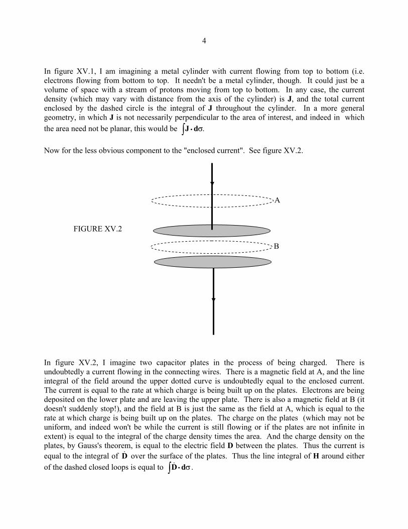
4 In figure XV.1, I am imagining a metal cylinder with current flowing from top to bottom (i.e. electrons flowing from bottom to top. It needn't be a metal cylinder, though. It could just be a volume of space with a stream of protons moving from top to bottom. In any case, the current density (which may vary with distance from the axis of the cylinder) is J, and the total current enclosed by the dashed circle is the integral of J throughout the cylinder. In a more general geometry, in which J is not necessarily perpendicular to the area of interest, and indeed in which the area need not be planar, this would be ∫ • .σdJ Now for the less obvious component to the "enclosed current". See figure XV.2. In figure XV.2, I imagine two capacitor plates in the process of being charged. There is undoubtedly a current flowing in the connecting wires. There is a magnetic field at A, and the line integral of the field around the upper dotted curve is undoubtedly equal to the enclosed current. The current is equal to the rate at which charge is being built up on the plates. Electrons are being deposited on the lower plate and are leaving the upper plate. There is also a magnetic field at B (it doesn't suddenly stop!), and the field at B is just the same as the field at A, which is equal to the rate at which charge is being built up on the plates. The charge on the plates (which may not be uniform, and indeed won't be while the current is still flowing or if the plates are not infinite in extent) is equal to the integral of the charge density times the area. And the charge density on the plates, by Gauss's theorem, is equal to the electric field D between the plates. Thus the current is equal to the integral of D& over the surface of the plates. Thus the line integral of H around either of the dashed closed loops is equal to .∫ • σdD&

A

B

FIGURE XV.2

5 In general, both types of current (the obvious one in which there is an obvious flow of charge, and the less obvious one, where the electric field is varying because of a real flow of charge elsewhere) contributes to the magnetic field, and so Ampère's theorem in general must read .)(

arealoopσdJDdsH •• ∫∫ += & 15.5.1

But the line integral of a vector field around a closed plane curve is equal to the surface integral of its curl, and therefore .)(

areaareaσσ dJDdH curl •• ∫∫ += & 15.5.2

Thus we arrive at: ,JDH curl += & 15.5.3 or, in the nabla notation, .JDH += &×∇ 15.5.4 This is the third of Maxwell's equations. 15.6 The Magnetic Equivalent of Poisson's Equation This deals with a static magnetic field, where there is no electrostatic field or at least any electrostatic field is indeed static – i.e. not changing. In that case curl H J= . Now the magnetic field can be derived from the curl of the magnetic vector potential, defined by the two equations B = curl A 15.6.1 and div A = 0. 15.6.2 (See Chapter 9 for a reminder of this.) Together with H = B/µ (µ = permeability), this gives us curl curl A J= µ . 15.6.3 If we now remind ourselves of the jabberwockian-sounding vector differential operator equivalence curl curl ≡ grad div − nabla-squared , 15.6.4 together with equation 15.6.2, this gives us ∇ = −2A Jµ . 15.6.5

6I don't know if this equation has any particular name, but it plays the same role for static magnetic fields that Poisson's equation plays for electrostatic fields. No matter what the distribution of currents, the magnetic vector potential at any point must obey equation 15.6.5 15.7 Maxwell's Fourth Equation This is derived from the laws of electromagnetic induction. Faraday's and Lenz's laws of electromagnetic induction tell us that the E.M.F. induced in a closed circuit is equal to minus the rate of change of B-flux through the circuit. The E.M.F. around a closed circuit is the line integral of E .ds around the circuit, where E is the electric field. The line integral of E around the closed circuit is equal to the surface integral of its curl. The rate of change of B-flux through a circuit is the surface integral of .B& Therefore ,BEcurl &−= 15.7.1 or, in the nabla notation, .BE &−=×∇ 15.7.2 This is the fourth of Maxwell's equations. 15.8 Summary of Maxwell's and Poisson's Equations

Maxwell's equations:

ρ=• D∇ 15.8.1 ∇• =B 0. 15.8.2

.JDH += &×∇ 15.8.3

.BE &−=×∇ 15.8.4

Sometimes you may see versions of these equations with factors such as 4π or c scattered liberally throughout them. If you do, my best advice is to white them out with a bottle of erasing fluid, or otherwise ignore them. I shall try to explain in Chapter 16 where they come from. They serve no scientific purpose, and are merely conversion factors between the many different systems of units that have been used in the past. Poisson's equation for the potential in an electrostatic field: ∇ = −2V ρ ε/ . 15.8.5

7The equivalent of Poisson's equation for the magnetic vector potential on a static magnetic field: ∇ = −2A Jµ . 15.8.6 15.9 Electromagnetic Waves Maxwell predicted the existence of electromagnetic waves, and these were generated experimentally by Hertz shortly afterwards. In addition, the predicted speed of the waves was 3 108× m s−1, the same as the measured speed of light, showing that light is an electromagnetic wave. In an isotropic, homogeneous, nonconducting, uncharged medium, where the permittivity and permeability are scalar quantities, Maxwell's equations can be written

0=• E∇ 15.9.1

0=• H∇ 15.9.2

.EH &ε=×∇ 15.9.3

.HE &µ−=×∇ 15.9.4 Take the curl of equation 15.9.3, and make use of equation 15.6.4:

grad H H curl Edivt

− ∇ =2 ε∂∂

. 15.9.5

Substitute for div H and curl E from equations 15.9.2 and 15.9.4 to obtain .2 HH &&εµ=∇ 15.9.6 Comparison with equation 15.1.2 shows that this is a wave of speed 1/ .εµ (Verify that this has the dimensions of speed.) In a similar manner the reader should easily be able to derive the equation

.2 EE &&εµ=∇ 15.9.7

In a vacuum, the speed is 1 0 0/ .ε µ With µ0 = 4π % 10−7 H m−1 and ε0 = 8.854 % 10−12 F m−1, this comes to 2.998 % 108 m s−1.

8

15.10 Gauge Transformations We recall (equation 9.1.1) that a static electric field E can be derived from the negative of the gradient of a scalar potential function of space: .VgradE −= 15.10.1 The zero of the potential is arbitrary. We can add any constant (with the dimensions of potential) to V. For example, if we define ,' CVV += where C is a constant (in the sense that it is not a function of x, y, z) then we can still calculate the electric field from '.VgradE −= We also recall (equation 9.2.1) that a static magnetic field B can be derived from the curl of a magnetic vector potential function: .AcurlB = 15.10.2 Let us also recall here the concept of the B-flux from equation 6.10.1: .B ∫∫ •=Φ AB d 15.10.3 It will be worth while here to recapitulate the dimensions and SI units of these quantities: E MLT−2Q−1 V m−1 B MT−1Q−1 T V ML2T−2Q−1 V A MLT−1Q−1 T m or Wb m−1 ΦΒ ML2T−1Q−1 T m2 or Wb Equation 15.10.2 is also true for a nonstatic field. Thus a time-varying magnetic field can be represented by the curl of a time-varying magnetic vector potential. However, we know from the phenomenon of electromagnetic induction that a varying magnetic field has the same effect as an electric field, so that, if the fields are not static, the electric field is the result of an electrical potential gradient and a varying magnetic field, so that equation 15.10.1 holds only for static fields. If we combine the Maxwell equation BEcurl &−= with the equation for the definition of the magnetic vector potential curl A = B, we obtain .)( 0AEcurl =+ & Then, since curl grad of any scalar function is zero, we can define a potential function V such that

9

.VgradAE −=+ & 15.10.4 (We could have chosen a plus sign, but we choose a minus sign so that it reduces to the familiar

VgradE −= for a static field.) Thus equations 15.10.4 and 15.10.2 define the electric and magnetic potentials – or at least they define the gradient of V and the curl of A. But we recall that, in the static case, we can add an arbitrary constant to V (as long as the constant is dimensionally similar to V), and the equation 'VgradE −= , where CVV +=' , still holds. Can we find a suitable transformation for V and A such that equations 15.10.2 and 15.10.4 still hold in the nonstatic case? Such a transformation would be a gauge transformation. Let χ be some arbitrary scalar function of space and time. I demand little of the form of χ; indeed I demand only two things. One is that it is a “well-behaved” function, in the sense that it is everywhere and at all times single-valued, continuous and differentiable. The other is that it should have dimensions ML2T−1Q−1. This is the same as the dimensions of magnetic B-flux, but I am not sure that it is particularly helpful to think of this. It will, however, be useful to note that the dimensions of grad χ and of χ& are, respectively, the same as the dimensions of magnetic vector potential (A) and of electric potential (V). Let us make the transformations χ−= gradAA' 15.10.5 and .' χ+= &VV 15.10.6 We shall see very quickly that this transformation (and we have a wide choice in the form of χ) preserves the forms of equations 15.10.2 and 15.10.4, and therefore this transformation (or, rather, these transformations, since χ can have any well-behaved form) are gauge transformations. Thus BAcurl = becomes .)( BgradA'curl =χ+ And since curl grad of any scalar field is zero, this becomes . BA'curl = Also, )AEgrad &+−= (V becomes .)('or,)()'( 'AEgradgrad'AEgrad &&&& +−=χ++−=χ− VV Thus the form of the equations is preserved. If we make a gauge transformation to the potentials such as equations 15.10.5 and 15.10.6, this does not change the fields E and B, so that the fields E and B are gauge invariant. Maxwell’s equations in their usual form are expressed in terms of E and B, and are hence gauge invariant.

1015.11 Maxwell’s Equations in Potential Form In their usual form, Maxwell’s equations for an isotropic medium, written in terms of the fields, are

ρ=Ddiv 15.11.1

0div =B 15.11.2

JDH curl += & 15.11.3

.BEcurl &−= 15.11.4 If we write the fields in terms of the potentials: VgradAE −−= & 15.11.5 and ,AcurlB = 15.11.6 together with D = εE and B = µH, we obtain for the first Maxwell equation, after some vector calculus and algebra,

' .)div(2

ερ

−=∂∂

+∇ At

V 15.11.7

For the second equation, we merely verify that zero is equal to zero. (div curl A = 0.) For the third equation, which requires a little more vector calculus and algebra, we obtain

' .div2

22 JAgradAA µ−

∂∂

εµ+=∂∂

εµ−∇tV

t 15.11.8

The speed of electromagnetic waves in the medium is ,/1 εµ and, in a vacuum, equation 15.11.8 becomes

' ,1div1022

2

22 JAgradAA µ−

∂∂

+=∂∂

−∇tV

ctc 15.11.9

where c is the speed of electromagnetic waves in a vacuum. The fourth Maxwell equation, when written in terms of the potentials, tells us nothing new (try it), so equations 15.11.7 and 15.11.8 (or 15.11.9 in vacuo) are Maxwell’s equations in potential form.

11These equations look awfully difficult – but perhaps we can find a gauge transformation, using some form for χ, and subtracting grad ξ from A and adding ξ& to V, which will make the equations much easier and which will still give the right answers for E and for B. One of the things that make equations 15.11.7 and 15.11.9 look particularly difficult is that each equation contains both A and V; that is, we have two simultaneous differential equations to solve for the two potentials. It would be nice if we had one equation for A and one equation for V. This can be achieved, as we shall shortly see, if we can find a gauge transformation such that the potentials are related by

.1div 2 tV

c ∂∂

−=A 15.11.10

You should check that the two sides of this equation are dimensionally similar. What would be the SI units? You’ll see that this is chosen so as to make the “difficult” part of equation 15.11.9 zero. If we make a gauge transformation and take the divergence of equation 15.10.5 and the time derivative of equation 15.10.6, we then see that condition 15.11.10 will be satisfied by a function χ that satisfies

.'1div122

2

22

tV

ctc ∂∂

−−=∂

ξ∂−ξ∇ A' 15.11.11

Don’t worry – you don’t have to solve this equation and find the function χ; you just have to be assured that some such function exists such that, when applied to the potentials, the potentials will be related by equation 15.11.10. Then, if you substitute equation 15.11.10 into Maxwell’s equations in potential form (equations 15.11.7 and 15.11.9), you obtain the following forms for Maxwell’s equations in vacuo in potential form, and the A and V are now separated:

' 0

2

2

22 1

ερ

−=∂∂

−∇tV

cV 15.11.12

and ' .102

2

22 JAA µ−=

∂∂

−∇tc

15.11.13

And, since these equations were arrived at by a gauge transformation, their solutions, when differentiated, will give the right answers for the fields.

1215.12 Retarded Potential In a static situation, in which the charge density ρ, the current density J, the electric field E and potential V, and the magnetic field B and potential A are all constant in time (i.e. they are functions of x, y and z but not of t) we already know how to calculate, in vacuo, the electric potential from the electric charge density and the magnetic potential from the current density. The formulas are

∫ρ

πε=

RdzyxzyxV ')',','(

41),,(

0

v 15.12.1

and .')',','(4

),,( 0 ∫πµ

=R

dzyxzyx vJA 15.12.2

Here R is the distance between the point )',','( zyx and the point ),,,( zyx and 'v is a volume element at the point )',','( zyx . I can’t remember if we have written these two equations in exactly that form before, but we have certainly used them, and given lots of examples of calculating V in Chapter 2, and one of calculating A in Section 9.3. The question we are now going to address is whether these formulas are still valid in a nonstatic situation, in which the charge density ρ, the current density J, the electric field E and potential V, and the magnetic field B and potential A are all varying in time (i.e. they are functions of x, y, z and t). The answer is “yes, but…”. The relevant formulas are indeed

∫ρ

πε=

RdtzyxtzyxV ')',',','(

41),,,(

0

v 15.12.3

and ,')',',','(4

),,,( 0 ∫πµ

=R

dtzyxtzyx vJA 15.12.4

…but notice the 't on the right hand side and the t on the left hand side! What this means is that, if

)',',','( tzyxρ is the charge density at a point )',','( zyx at time 't , equation 15.12.3 gives the correct potential at the point )',','( zyx at some slightly later time t, the time difference 'tt − being equal to the time R/c that it takes for an electromagnetic signal to travel from )',','( zyx to ),,( zyx . If the charge density at )',','( zyx changes, the information about this change cannot reach the point instantaneously; it takes a time R/c for the information to be transmitted from one point to another. The same considerations apply to the change in the magnetic potential when the current density changes, as described by equation 15.12.4. The potentials so calculated are called, naturally, the retarded potentials. While this result has been arrived at by a qualitative argument, in fact equations 15.12.3 and 4 can be obtained as a solution of the differential equations 15.11.12 and 13. Mathematically there is also a solution that gives an “advance potential” – that is, one in which

tt −' rather than 'tt − is equal to R/c. You can regard, if you wish, the retarded solution as the “physically acceptable” solution and discard the “advance” solution as not being physically significant. That is, the potential cannot predict in advance that the charge density is about to

13change, and so change its value before the charge density does. Alternatively one can think that the laws of physics, from the mathematical view at least, allow the universe to run equally well backward as well as forward, though in fact the arrow of time is such that cause must precede effect (a condition which, in relativity, leads to the conclusion that information cannot be transmitted from one place to another at a speed faster than the speed of light). One is also reminded that the laws of physics, from the mathematical view at least, allow the entropy of an isolated thermodynamical system to decrease (see Section 7.4 in the Thermodynamics part of these notes) – although in the real universe the arrow of time is such that the entropy in fact increases. Recall also the following passage from Through the Looking-glass and What Alice Found There. Alice was just beginning to say, "There's a mistake somewhere -- -" when the Queen began screaming, so loud that she had to leave the sentence unfinished. "Oh, oh, oh!" shouted the Queen, shaking her hand about as if she wanted to shake it off. "My finger's bleeding! Oh, oh, oh, oh!"

Her screams were so exactly like the whistle of a steam-engine, that Alice had to hold both her hands over her ears.

"What is the matter?" she said, as soon as there was a chance of making herself heard. "Have you pricked your finger?"

"I haven't pricked it yet" the Queen said, "but I soon shall -- -oh, oh, oh!"

"When do you expect to do it?" Alice asked, feeling very much inclined to laugh.

"When I fasten my shawl again," the poor Queen groaned out: "the brooch will come undone directly. Oh, oh!" As she said the words the brooch flew open, and the Queen clutched wildly at it, and tried to clasp it again.

"Take care!" cried Alice. "You're holding it all crooked!" And she caught at the brooch; but it was too late: the pin had slipped, and the Queen had pricked her finger.

"That accounts for the bleeding, you see," she said to Alice with a smile. "Now you understand the way things happen here."

"But why don't you scream now?" Alice asked, holding her hands ready to put over her ears again. "Why, I've done all the screaming already," said the Queen. "What would be the good of having it all over again?"

Addendum. Coincidentally, just two days after having completed this chapter, I received the 2005 February issue of Astronomy & Geophysics, which included a fascinating article on the Arrow of Time. You might want to look it up. The reference is Davis, P., Astronomy & Geophysics (Royal Astronomical Society) 46, 26 (2005).

1-CHAPTER 16

CGS ELECTRICITY AND MAGNETISM 16.1 Introduction We are accustomed to using MKS (metre-kilogram-second) units. A second, at one time defined as a fraction 1/86400 of a day, is now defined as 9 192 631 770 times the period of a hyperfine line emitted in the spectrum of the 133Cs (caesium) atom. A metre was at one time defined as one ten-millionth of the length of a quadrant of Earth's surface measured from pole to equator. Later it was defined as the distance between two scratches on a platinum-iridium bar held on Paris. Still later, it was defined in terms of the wavelength of one or other of several spectral lines that have been used in the past for this purpose. At present, the metre is defined as the distance travelled by light in vacuo in a time of 1/(299 792 458) second. A kilogram is equal to the mass of a platinum-iridium cylinder held in Paris. The day may come when we are able to define a kilogram as the mass of so many electrons, but that day is not yet. For electricity and magnetism, we extended the MKS system by adding an additional unit, the ampère, whose definition was given in Chapter 6, Section 6.2, to form the MKSA system. This in turn is a subset of SI (le Système International des Unités), which also includes the kelvin, the candela and the mole. An older system of units, still used by some authors, was the CGS (centimetre-gram-second) system. In this system, a dyne is the force that will impart an acceleration of 1 cm s−2 to a mass of 1 gram. An erg is the work done when a force of one dyne moves its point of application through 1 cm in the line of action of the force. It will not take the reader a moment to see that a newton is equal to 105 dynes, and a joule is 107 ergs. As far as mechanical units are concerned, neither one system has any particular advantage over the other. When it comes to electricity and magnetism, however, the situation is entirely different, and there is a huge difference between MKS and CGS. Part of the difficulty stems from the circumstance that electrostatics, magnetism and current electricity originally grew up as quite separate disciplines, each with its own system of units, and the connections between them were not appreciated or even discovered. It is not always realized that there are several version of CGS units used in electricity and magnetism, including hybrid systems, and countless conversion factors between one version and another. There are CGS electrostatic units (esu), to be used in electrostatics; CGS electromagnetic units (emu), to be used for describing magnetic quantities; and gaussian mixed units. In the gaussian mixed system, in equations that include both electrostatic quantities and magnetic quantities, the former were supposed to be expressed in esu and the latter in emu, and a conversion factor, given the symbol c, would appear in various parts of an equation to take account of the fact that some quantities were expressed in one system of units and others were expressed in another system. There was also the practical system of units, used in current electricity. In this, the ampère would be defined either in terms of the rate of electrolytic deposition of silver from a silver nitrate solution, or as exactly 10 CGS emu of current. The ohm would be defined in terms of the resistance of a column of mercury of defined dimensions, or again as exactly 109 emu of resistance. And a volt was 108 emu of potential difference. It will be seen already that, for every

2electrical quantity, several conversion factors between the different systems had to be known. Indeed, the MKSA system was devised specifically to avoid this proliferation of conversion factors. Generally, the units in these CGS system have no particular names; one just talks about so many esu of charge, or so many emu of current. Some authors, however, give the names statcoulomb, statamp, statvolt, statohm ,etc., for the CGS esu of charge, current, potential difference and resistance, and abcoulomb, abamp, abvolt, abohm for the corresponding emu. The difficulties by no means end there. For example, Coulomb's law is generally written as

.2

21

krQQF = 16.1.1

It will immediately be evident from this that the permittivity defined by this equation differs by a factor of 4π from the permittivity that we are accustomed to. In the familiar equation generally used in conjunction with SI units, namely

F Q Qr

= 1 224πε

, 16.1.2

the permittivity ε so defined is called the rationalized permittivity. The permittivity k of equation16.1.1 is the unrationalized permittivity. The two are related by .4πε=k A difficulty with the unrationalized form is that a factor 4π appears in formulas describing uniform fields, and is absent from formulas describing situations with spherical symmetry. Yet a further difficulty is that the magnitude of the CGS esu of charge is defined in such a way that the unrationalized free space permittivity has the numerical value 1 – and consequently it is normally left out of any equations in which it should appear. Thus equations as written often do not balance dimensionally, and one is deprived of dimensional analysis as a tool. Permittivity is regarded as a dimensionless number, and Coulomb's law for two charges in vacuo is written as

F Q Qr

= 1 22

. 16.1.3

The view is taken that electrical quantities can be expressed dimensionally in terms of mass, length and time only, and, from equation 16.1.3, it is asserted that the dimensions of electrical charge are [ ] ./ /Q = −M L T1 2 3 2 1 16.1.4 Because permittivity is regarded as a dimensionless quantity, the vectors E and D are regarded as dimensionally similar, and in vacuo they are identical. That is, in vacuo, there is no distinction between them. When we come to CGS electromagnetic units all these difficulties reappear, except that, in the emu system, the free space permeability is regarded as a dimensionless number equal to 1, B and H are

3dimensionally similar, and in vacuo there is no distinction between them. The dimensions of electric charge in the CGS emu system are [ ] ./ /Q = M L1 2 1 2 16.1.5 Thus the dimensions of charge are different in esu and in emu. Two more highlights. The unit of capacitance in the CGS system is the centimeter, but in the CGS emu system, the centimetre is the unit of inductance. Few users of CGS esu and emu fully understand the complexity of the system. Those who do so have long abandoned it for SI. CGS units are probably largely maintained by those who work with CGS units in a relatively narrow field and who therefore do not often have occasion to convert from one unit to another in this immensely complicated and physically unrealistic system. Please don't blame me for this – I'm just the messenger! In Sections 16.2, 16.3 and 16.4 I shall describe some of the features of the esu, emu and mixed systems. I shall not be giving a full and detailed exposition of CGS electricity, but I am just mentioning some of the highlights and difficulties. You are not going to like these sections very much, and will probably not make much sense of them. I suggest just skip through them quickly the first time, just to get some idea of what it's all about. The practical difficulty that you are likely to come across in real life is that you will come across equations and units written in CGS language, and you will want to know how to translate them into the SI language with which you are familiar. I hope to address that in Section 16.5, and to give you some way of translating a CGS formula into an SI formula that you can use and get the right answer from. 16.2 The CGS Electrostatic System Definition. One CGS esu of charge (also known as the statcoulomb) is that charge which, if placed 1 cm from a similar charge in vacuo, will repel it with a force of 1 dyne. The following exercises will be instructive. Calculate, from the SI electricity that you already know, the force between two coulombs placed 1 cm from each other. From this, calculate how many CGS esu of charge there are in a coulomb. (I make it 1 coulomb = 2 998 109. × esu. It will not escape your notice that this number is ten times the speed of light expressed in m s−1.) Calculate the magnitude of the electronic charge in CGS esu. (I make it 4 8 10 10. × − esu. If, for example, you see that the potential energy of two electrons at a distance r apart is e2/r, this is the number you must substitute for e. If you then express r in cm, the energy will be in ergs.)

4Coulomb's law in vacuo is

F Q Qr

= 1 22

, 16.2.1

This differs from our accustomed formula (equation 16.1.2) in two ways. In the first place, we are using an unrationalized definition of permittivity, so that the familiar 4π is absent. Secondly, we are choosing units such that 4πε0 has the numerical value 1, and so we are omitting it from the equation. While some readers (and myself!) will object, and say that equation 16.2.1 does not balance dimensionally, and is valid only if the quantities are expressed in particular units, others will happily say that equation 16.2.1 shows that the dimensions of Q are M1/2L3/1T−1, and will not mind these extraordinary dimensions. Electric field E is defined in the usual way, i.e. F = QE, so that if the force on 1 esu of charge is 1 dyne, the field strength is 1 esu of electric field. (The esu of electric field has no name other than esu.) This is fine, but have you any idea how this is related to the SI unit of E, volt per metre? It requires a great deal of mental gymnastics to find out, so I'll just give the answer here, namely

1 CGS esu of E = 10−6c V m−1,

where c = 2.997 924 58 % 1010. Now the vector D is defined by D = kE, and since the permittivity is held to be a dimensionless number, D and E are held to be dimensionally similar (M1/2L−1/2T−1 in fact). Further, since the free space permittivity is 1, in vacuo there is no distinction between D and E, and either can substitute for the other. So the conversion between CGS esu and SI for D is the same as for E? No! In SI, we recognize D and E as being physically different quantities, and D is expressed in coulombs per square metre. Awful mental gymnastics are needed to find the conversion, but I'll give the answer here:

1 CGS esu of D = 104

5

πc C m−2.

Once again, please don't blame me – I'm just the messenger! And be warned – it is going to get worse – much worse. Potential Difference If the work required to move a charge of 1 esu from one point to another is 1 erg, the potential difference between the points is 1 esu of potential difference, or 1 statvolt. It is often said that an esu of potential difference is 300 volts, but this is just an approximation. The exact conversion is

5

1 statvolt = 10−8c V. Capacitance If the potential difference across the plate of a capacitor is one statvolt when the capacitor holds a charge of one statcoulomb, the capacitance of the capacitor is one centimetre. (No – that's not a misprint.)

1 cm = 109 c−2 F. Here is a sample of some formulas for use with CGS esu. Potential at a distance r from a point charge Q in vacuo = Q/r. Field at a distance r in vacuo from an infinite line charge of λ esu/cm = 2λ/r. Field in vacuo above an infinite charged plate bearing a surface charge density of σ esu/cm2 = 2πσ. An electric dipole moment p is, as in SI, the maximum torque experienced by the dipole in unit electric field. A debye is 10−18 esu of dipole moment. The field at a distance r in vacuo along the axis of a dipole is 2p/r. Gauss's theorem: The total normal outward flux through a closed surface is 4π time the enclosed charge.

Capacitance of a plane parallel capacitor = .4 dkAπ

Capacitance of an isolated sphere of radius a in vacuo = a. Example: What is the capacitance of a sphere of radius 1 cm? Answer: 1 cm. Easy, eh? Energy per unit volume or an electric field = E2/(8π). One more example before leaving esu. You will recall that, if a polarizable material is placed in an electrostatic field, the field D in the material is greater than ε0E by the polarization P of the material. That is, D = εE + P. The equivalent formula for use with CGS esu is

D = E + 4πP.

And since P = χeE and D = kE, it follows that

k = 1 + 4πχe.

6At this stage you may want a conversion factor between esu and SI for all quantities. I'll supply one a little later, but I want to describe emu first, and then we can construct a table given conversions between all three systems. 16.3 The CGS Electromagnetic System If you have been dismayed by the problems of CGS esu, you don't yet know what is in store for you with CGS emu. Wait for it: Definition. One CGS emu of magnetic pole strength is that pole which, if placed 1 cm from a similar pole in vacuo, will repel it with a force of 1 dyne. The system is based on the proposition that there exists a "pole" at each end of a magnet, and that point poles repel each other according to an inverse square law. Magnetic field strength H is defined as the force experienced by a unit pole situated in the field. Thus, if a pole of strength m emu is situated in a field of strength H, it will experience a force F = mH. Definition. If a pole of strength 1 emu experiences a force of 1 dyne when it is situated in a magnetic field, the strength of the magnetic field is 1 oersted (Oe). It will probably be impossible for the reader at this stage to try to work out the conversion factor between Oe and A m−1, but, for the record

1 Oe = 250π

A m−1.

Now hold on tight, for the definition of the unit of electric current. Definition: One emu of current (1 abamp) is that steady current, which, flowing in the arc of a circle of length 1 cm and of radius 1 cm (i.e. subtending 1 radian at the centre of the circle) gives rise to a magnetic field of 1 oersted at the centre of the circle. This will involve quite an effort of the imagination. First you have to imagine a current flowing in an arc of a circle. Then you have to imagine measuring the field at the centre of the circle by measuring the force on a unit magnetic pole that you place there. It follows that, if a current I abamp flows in a circle of radius a cm, the field at the centre is of the circle is

H Ia

=2π Oe.

The conversion between emu of current (abamp) and ampères is

1 emu = 10 A.

7The Biot-Savart law becomes

dH I dsr

=sin .θ2

The field at a distance r in vacuo from a long straight current I is

H Ir

=2 .

Ampère's law says that the line integral of H around a closed plane curve is 4π times the enclosed current. The field inside a long solenoid of n turns per centimetre is

H = 4πnI. So far, no mention of B, but it is now time to introduce it. Let us imagine that we have a long solenoid of n turns per cm, carrying a current of I emu, so that the field inside it is 4πnI Oe. Suppose that the cross-sectional area of the solenoid is A. Let us wrap a single loop of wire tightly around the outside of the solenoid, and then change the current at a rate I& so that the field changes at a rate .4 InH && π= An EMF will be set up in the outside (secondary) coil of magnitude .HA & If we now insert an iron core inside the solenoid and repeat the experiment, we find that the induced EMF is much larger. It is larger by a (supposed dimensionless) factor called the permeability of the iron. Although this factor is called the permeability and the symbols used is often µ, I am going to use the symbol κ for it. The induced EMF is now A times .H&κ We denote the product of µ and H with the symbol B, so that B = κH. The magnitude of B inside the solenoid is

B = 4πκnI.

It will be evident from the familiar SI version B = µnI that the CGS emu definition of the permeability differs from the SI definition by a factor 4π. The CGS emu definition is called an unrationalized definition; the SI definition is rationalized. The relation between them is µ = 4πκ. In CGS emu, the permeability of free space has the value 1. Indeed the supposedly dimensionless unrationalized permeability is what, in SI parlance, would be the relative permeability. The CGS unit of B is the gauss (G), and 1 G = 10−4 T. It is usually held that κ is a dimensionless number, so that B and H have the same dimensions, and, in free space, B and H are identical. They are identical not only numerically, but there is physically no distinction between them. Because of this, the unit oersted is rarely heard, and it is common to hear the unit gauss used haphazardly to describe either B or H. The scalar product of B and area is the magnetic flux, and its CGS unit, G cm2, bears the name the maxwell. The rate of change of flux in maxwells per second will give you the induced EMF in emus (abvolts). An abvolt is 10−8 V.

8 The subject of magnetic moment has caused so much confusion in the literature that I shall devote an entire future chapter to it rather than try to do it here. I end this section by giving the CGS emu version of magnetization. The familiar B H M= +µ0 ( ) becomes, in its CGS emu guise, B H M= + 4π . The magnetic susceptibility χm is defined by M = χmH . Together with B = κH, this results in κ = 1 + 4πχm . 16.4 The Gaussian Mixed System A problem arises if we are dealing with a situation in which there are both “electrostatic” and “electromagnetic” quantities. The “mixed system”, which is used very frequently, in CGS literature, uses esu for quantities that are held to be “electrostatic” and emu for quantities that are held to be “electromagnetic”, and it seems to be up to each author to decide which quantities are to be regarded as “electrostatic” and which are “electromagnetic. Because different quantities are to be expressed in different sets of units within a single equation, the equation must include the conversion factor c = 2.997 924 58 % 1010 in strategic positions within the equation. The most familiar example of this is the equation for the force F experienced by a charge Q when it is moving with velocity v in an electric field E and a magnetic field B. This equation is liable to appear either as

+=

cQF HvE × 16.4.1

or as .

+=

cQF BvE × 16.4.2

It can appear in either of these forms because, if CGS emu are used, B and H are numerically equal in vacuo. The conversion factor c appears in these equations, because it is understood (by those who understand CGS units) that Q and E are to be expressed in esu, while B or H is to be expressed in emu, and the conversion factor c is necessary to convert it to esu. It should be noted that in all previous chapters in these notes, equations balance dimensionally, and the equations are valid in any coherent system of units, not merely SI. Difficulties arise, of course, if you write an equation that is valid only so long as a particular set of units is used, and even more difficulties arise if some quantities are to be expressed in one system of units, and other quantities are to be expressed in another system of units. An analogous situation is to be found in some of the older books on thermodynamics, where it is possible to find the following equation: ./ JRCC VP =− 16.4.3

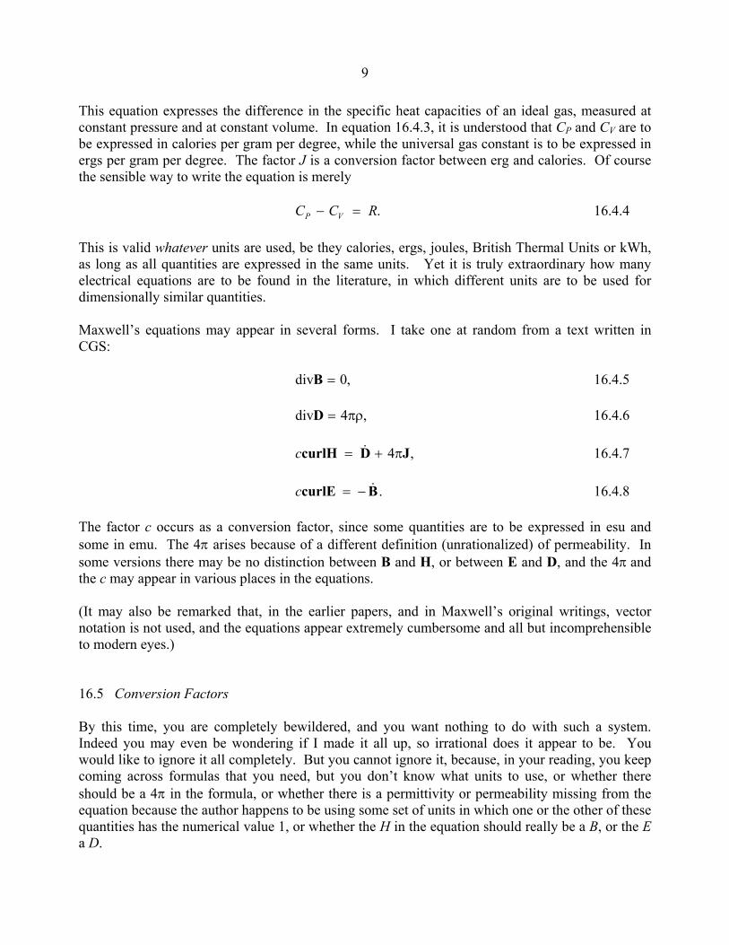
9 This equation expresses the difference in the specific heat capacities of an ideal gas, measured at constant pressure and at constant volume. In equation 16.4.3, it is understood that CP and CV are to be expressed in calories per gram per degree, while the universal gas constant is to be expressed in ergs per gram per degree. The factor J is a conversion factor between erg and calories. Of course the sensible way to write the equation is merely .RCC VP =− 16.4.4 This is valid whatever units are used, be they calories, ergs, joules, British Thermal Units or kWh, as long as all quantities are expressed in the same units. Yet it is truly extraordinary how many electrical equations are to be found in the literature, in which different units are to be used for dimensionally similar quantities. Maxwell’s equations may appear in several forms. I take one at random from a text written in CGS: ,0div =B 16.4.5 ,4div πρ=D 16.4.6 ,4 JDcurlH π+= &c 16.4.7 .BcurlE &−=c 16.4.8 The factor c occurs as a conversion factor, since some quantities are to be expressed in esu and some in emu. The 4π arises because of a different definition (unrationalized) of permeability. In some versions there may be no distinction between B and H, or between E and D, and the 4π and the c may appear in various places in the equations. (It may also be remarked that, in the earlier papers, and in Maxwell’s original writings, vector notation is not used, and the equations appear extremely cumbersome and all but incomprehensible to modern eyes.) 16.5 Conversion Factors By this time, you are completely bewildered, and you want nothing to do with such a system. Indeed you may even be wondering if I made it all up, so irrational does it appear to be. You would like to ignore it all completely. But you cannot ignore it, because, in your reading, you keep coming across formulas that you need, but you don’t know what units to use, or whether there should be a 4π in the formula, or whether there is a permittivity or permeability missing from the equation because the author happens to be using some set of units in which one or the other of these quantities has the numerical value 1, or whether the H in the equation should really be a B, or the E a D.

10 Is there anything I can do to help? What I am going to do in this section is to list a number of conversion factors between the different systems of units. This may help a little, but it won’t by any means completely solve the problem. Really to try and sort out what a CGS equation means requires some dimensional analysis, and I shall address that in section 16.6 In the conversion factors that I list in this section, the symbol c stands for the number 2.997 924 58 % 1010, which is numerically equal to the speed of light expressed in cm s−1. The abbreviation “esu” will mean CGS electrostatic unit, and “emu” will mean CGS electromagnetic unit. A prefix “stat” to a unit implies that it is an esu; a prefix “ab” implies that it is an emu. I list the conversion factors for each quantity in the form “1 SI unit = so many esu = so many emu”. I might mention that people will say that “SI is full of conversion factors”. The fact is that SI is a unified coherent set of units, and it has no conversion factors. Conversion factors are characteristic of CGS electricity and magnetism. Quantity of Electricity (Electric Charge) 1 coulomb = 10−1c statcoulomb = 10−1 emu Electric Current 1 amp = 10−1c esu = 10−1 abamp Potential Difference 1 volt = 108/c statvolt = 108 emu Resistance 1 ohm = 109/c2 esu = 109 abohm Capacitance 1 farad = 10−9c2 esu = 10−9 emu Inductance 1 henry = 109/c2 esu = 109 emu

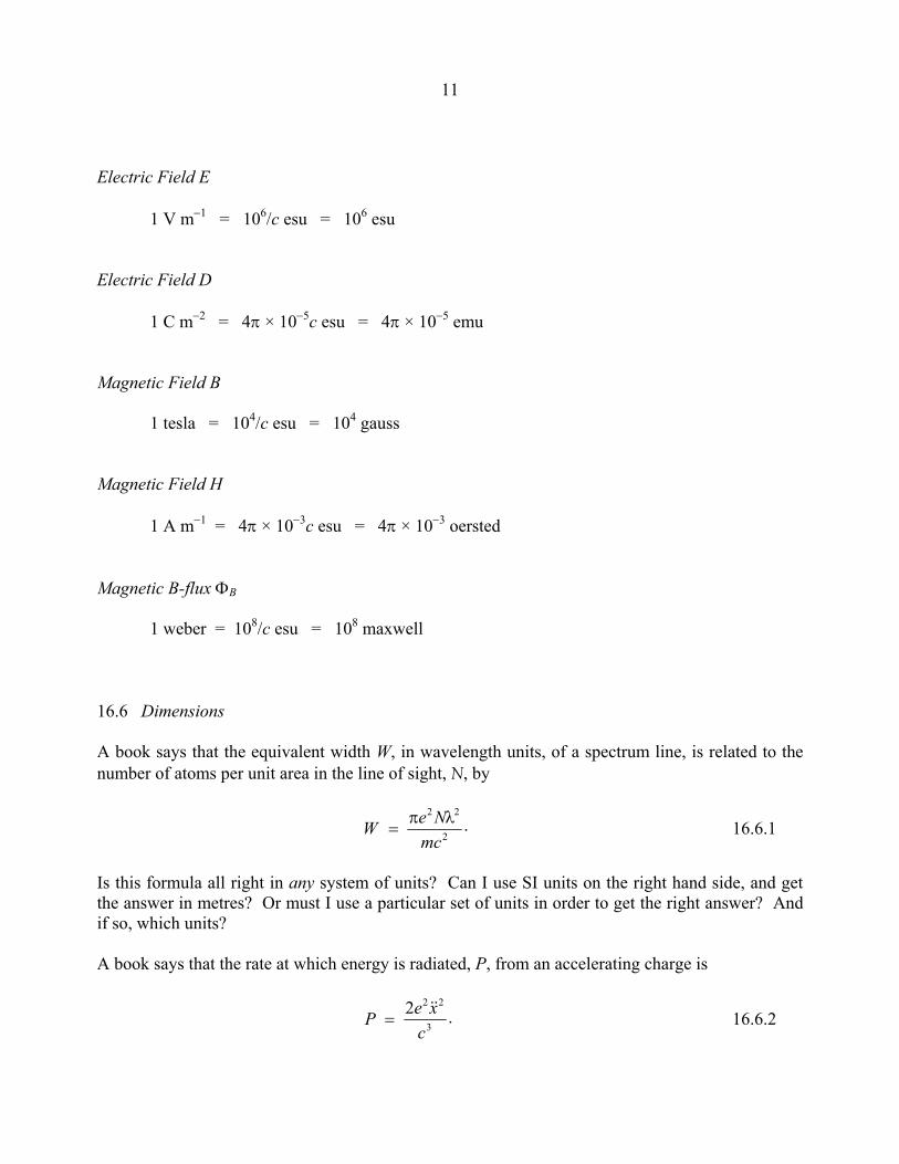
11 Electric Field E 1 V m−1 = 106/c esu = 106 esu Electric Field D 1 C m−2 = 4π × 10−5c esu = 4π × 10−5 emu Magnetic Field B 1 tesla = 104/c esu = 104 gauss Magnetic Field H 1 A m−1 = 4π × 10−3c esu = 4π × 10−3 oersted Magnetic B-flux ΦB

1 weber = 108/c esu = 108 maxwell 16.6 Dimensions A book says that the equivalent width W, in wavelength units, of a spectrum line, is related to the number of atoms per unit area in the line of sight, N, by

.2

22

mceW λπ

=N 16.6.1

Is this formula all right in any system of units? Can I use SI units on the right hand side, and get the answer in metres? Or must I use a particular set of units in order to get the right answer? And if so, which units? A book says that the rate at which energy is radiated, P, from an accelerating charge is

.23

22

cxeP&&

= 16.6.2

12 Is this correct? Is c the speed of light, or is it merely a conversion factor between different units? Or is one of the cs a conversion factor, and the other two are the speed of light? It is possible to find the answer to such bewildering questions, if we do a bit of dimensional analysis. So, before trying to answer these specific questions (which I shall do later as examples) I am going to present a table of dimensions. I already gave a table of dimensions of electrical quantities in Chapter 11, in terms of M, L, T and Q, but that table won’t be particularly helpful in the present context. I pointed out in Section 16.1 of the present chapter that Coulomb’s law is often written in the form

F Q Qr

= 1 22

. 16.6.3

Consequently the dimensions of Q are held to be [ ] ./ /Q = −M L T1 2 3 2 1 But we know that a permittivity is missing from the denominator of equation 16.6.3, because the writer intends his formula to be restricted to a particular set of units such that k or 4πε0 = 1. In order to detect whether a permittivity has been omitted from an equation, we need a table in which the dimensions of electrical quantities are given not in terms of M, L, T and Q as in Chapter 11, but in terms of M, L, T and ε, and this is what I am just about to do. However, often it is the permeability that has been omitted from an equation, and, in order to detect whether this is so, I am also supplying a table in which the dimensions of electrical quantities are given in terms of M, L, T and µ. If, from dimensional analysis, you find that an expression is dimensionally wrong by a power of the permittivity, insert 4πε0 in the appropriate part of the equation. If you find that an expression is dimensionally wrong by a power of the permeability, insert µ0/(4π) in the appropriate part of the equation. If you find that the equation is wrong by LT−1, insert or delete c as appropriate. Your equation will then balance dimensionally and will be ready for use in any coherent system of units, including SI. This procedure will probably work in most cases, but I cannot guarantee that it will work in all cases, because it cannot deal with those (frequent!) cases in which the formula given is plain wrong, whatever units are used!

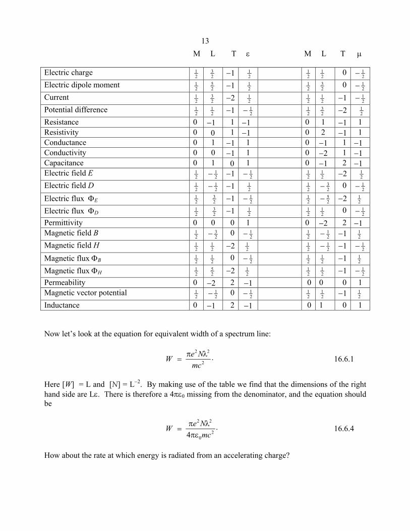
13 M L T ε M L T µ Electric charge 2

1 23 −1 2

1 21 2

1 0 21−

Electric dipole moment 21 2

5 −1 21 2

1 23 0 2

1−Current 2

1 23 −2 2

1 21 2

1 −1 21−

Potential difference 21 2

1 −1 21− 2

1 23 −2 2

1 Resistance 0 −1 1 −1 0 1 −1 1 Resistivity 0 0 1 −1 0 2 −1 1 Conductance 0 1 −1 1 0 −1 1 −1 Conductivity 0 0 −1 1 0 −2 1 −1 Capacitance 0 1 0 1 0 −1 2 −1 Electric field E 2

121− −1 2

1− 21 2

1 −2 21

Electric field D 21

21− −1 2

1 21 2

3− 0 21−

Electric flux ΦE 21 2

3 −1 21− 2

1 25− −2 2

1 Electric flux ΦD 2

1 23 −1 2

1 21 2

1 0 21−

Permittivity 0 0 0 1 0 −2 2 −1 Magnetic field B 2

123− 0 2

1− 21 2

1− −1 21

Magnetic field H 21 2

1 −2 21 2

1 21− −1 2

1−

Magnetic flux ΦB 21 2

1 0 21− 2

1 21 −1 2

1 Magnetic flux ΦH 2

1 25 −2 2

1 21 2

1 −1 21−

Permeability 0 −2 2 −1 0 0 0 1 Magnetic vector potential 2

121− 0 2

1− 21 2

1 −1 21

Inductance 0 −1 2 −1 0 1 0 1 Now let’s look at the equation for equivalent width of a spectrum line:

.2

22

mceW λπ

=N 16.6.1

Here [W] = L and [N] = L−2. By making use of the table we find that the dimensions of the right hand side are Lε. There is therefore a 4πε0 missing from the denominator, and the equation should be

.4 2

0

22

mceW

πελπ

=N 16.6.4

How about the rate at which energy is radiated from an accelerating charge?

14

.23

22

cxeP&&

= 16.6.2

Power has dimensions ML2T−3, whereas the dimensions of the right hand side are ML2T−3ε, so again there is a 4πε0 missing from the denominator and the formula should be

.42

30

22

cxeP

πε=

&& 16.6.5

It is often the case that there is a 4πε0 missing from the denominator is formulas that have an e2 upstairs. “Electromagnetic” formulas often give more difficulty. For example, one book says that the energy

per unit volume in a magnetic field in vacuo is π8

2B , while another says that is it is .8

2

πH Which is it

(if indeed it is either)? Energy per unit volume has dimensions ML−1T−2. The dimensions of B2 are ML−1T−2µ. The equation given is therefore wrong dimensionally by permeability, and the equation should be divided by µ0/(4π) to give B2/(2µ0), which is correct. On the other hand, the dimensions of H2 are ML−1T−2µ−1, so perhaps we should multiply by µ0/(4π)? But this does not give a correct answer, and it exemplifies some of the many difficulties that are caused by writing formulas that do not balance dimensionally and are intended to be used only with a particular set of units. The situation is particularly difficult with respect to magnetic moment, a subject to which I shall devote the next chapter.

1

CHAPTER 17 MAGNETIC DIPOLE MOMENT

17.1 Introduction A number of different units for expressing magnetic dipole moment (hereafter simply “magnetic moment”) are commonly seen in the literature, including, for example, erg G−1, G cm3, Oe cm3, T m3, A m2, J T−1. It is not always obvious how to convert from one to another, nor is it obvious whether all quantities described as “magnetic moment” refer to the same physical concept or are dimensionally or numerically similar. It can be almost an impossibility, for example, to write down a list of the magnetic moments of the planets in order of increasing magnetic moment if one refers to the diverse literature in which the moments of each of the nine planets are quoted in different units. This chapter explores some of these aspects of magnetic moment. In previous chapters, I have used the symbols pe and pm for electric and magnetic dipole moment. In this chapter I shall be concerned exclusively with magnetic moment, and so I shall dispense with the subscript m. 17.2 The SI Definition of Magnetic Moment If a magnet is placed in an external magnetic field B, it will experience a torque. The magnitude of the torque depends on the orientation of the magnet with respect to the magnetic field. There are two oppositely-directed orientations in which the magnet will experience the greatest torque, and the magnitude of the magnetic moment is defined as the maximum torque experienced by the magnet when placed in unit external magnetic field. The magnitude and direction of the torque is given by the equation .Bp×τ = 17.2.1 The SI unit for magnetic moment is clearly N m T−1. If an electric current I flows in a plane coil of area A (recall that area is a vector quantity – hence the boldface), the torque it will experience in a magnetic field is given by .BAτ ×= I 17.2.2 This means that the magnetic moment of the coil is given by .Ap I= 17.2.3 Thus the unit A m2 is also a correct SI unit for magnetic moment, though, unless the concept of “current in a coil” needs to be emphasized in a particular context, it is perhaps better to stick to N m T−1.

2

While “J T−1” is also formally dimensionally correct, it is perhaps better to restrict the unit “joule” to work or energy, and to use N m for torque. Although these are dimensionally similar, they are conceptually rather different. For this reason, the occasional practice seen in atomic physics of expressing magnetic moments in MeV T−1 is not entirely appropriate, however convenient it may sometimes seem to be in a field in which masses and momenta are often conveniently expressed in MeV/c2 and MeV/c. It is clear that the unit “T m3”, often seen for “magnetic moment” is not dimensionally correct for magnetic moment as defined above, so that, whatever quantity is being expressed by the often-seen “T m3”, it is not the conventionally defined concept of magnetic moment. The magnetization M of a material is defined by the equation B = µ0(H + M) 17.2.4 Equations 17.2.2 and 17.2.4 for the definitions of magnetic moment and magnetization are consistent with the alternative concept of magnetization as “magnetic moment per unit volume”. 17.3 The Magnetic Field on the Equator of a Magnet By the “equator” of a magnet I mean a plane normal to its magnetic moment vector, passing through the mid-point of the magnet. The magnetic field at a point at a distance r on the equator of a magnet may be expressed as a series of terms of successively higher powers of 1/r (the first term in the series being a term in r−3), and the higher powers decrease rapidly with increasing distance. At large distances, the higher powers become negligible, so that, at a large distance from a small magnet, the magnitude of the magnetic field produced by the magnet is given approximately by

.4 3

0

rpB

πµ

= 17.3.1

For example, if the surface magnetic field on the equator of a planet has been measured, and the magnetic properties of the planet are being modelled in terms of a small magnet at the centre of the planet, the dipole moment can be calculated by multiplying the surface equatorial magnetic field by µ0/(4π) times the cube of the radius of the planet. If B, µ0 and r are expressed respectively in T, H m−1 and m, the magnetic moment will be in N m T−1.

3

17.4 CGS Magnetic Moment, and Lip Service to SI Equation 17.3.1 is the equation (written in the convention of quantity calculus, in which symbols stand for physical quantities rather than for their numerical values in some particular system of units) for the magnetic field at a large distance on the equator of a magnet. The equation is valid in any coherent system of units whatever, and its validity is not restricted to any particular system of units. Example of systems of units in which equation 17.3.1 are valid include SI, CGS EMU, and British Imperial Units. If CGS EMU are used, the quantity µ0/(4π) has the numerical value 1. Consequently, when working exclusively in CGS EMU, equation 17.3.1 is often written as

.3rpB = 17.4.1

This equation appears not to balance dimensionally. However, the equation is not written according to the conventions of quantity calculus, and the symbols do not stand for physical quantities. Rather, they stand for their numerical values in a particular system of units. Thus r is the distance in cm, B is the field in gauss, and p is the magnetic moment in dyne cm per gauss. However, because of the deceptive appearance of the equation, a common practice, for example, in calculating the magnetic moment of a planet is to measure its surface equatorial field, multiply it by the cube of the planet’s radius, and then quote the magnetic moment in “G cm3”. While the numerical result is correct for the magnetic moment in CGS EMU, the units quoted are not. While some may consider objections to incorrect units to be mere pedantry (and who would presumably therefore see nothing wrong with quoting a length in grams, as long as the actual number is correct), the situation becomes more difficult when a writer, wishing to pay lip service to SI, attempts to use equation 17.4.1 using SI units, by multiplying the surface equatorial field in T by the cube of the planet’s radius, and then giving the magnetic moment in “T m3”, a clearly disastrous recipe! Of course, some may use equation 17.4.1 as a definition of magnetic moment. If that is so, then the quantity so defined is clearly not the same quantity, physically, conceptually, dimensionally or numerically, as the quantity defined as magnetic moment in Section 17.2. 17.5 Possible Alternative Definitions of Magnetic Moment Although the standard SI definition of magnetic moment is described in Section 17.2, and there is little reason for anyone who wishes to be understood by others to use any other, the previous paragraph suggested that there might be more than one choice as to how one wishes to define magnetic moment. Do we use equation 17.2.1 or equation 17.4.1 as the definition? (They are clearly different concepts.) Additional degrees of freedom as to how one might choose to define magnetic moment depend on whether we elect to use

4

magnetic field H or magnetic field B in the definition, or whether the permeability is or is not to include the factor 4π in its definition – that is, whether we elect to use a “rationalized” or “unrationalized” definition of permeability. If one chooses to define the magnetic moment as the maximum torque experienced in unit external magnetic field, there is still a choice as to whether by magnetic field we choose H or B. Thus we could define magnetic moment by either of the following two equations: Hp1=τ 17.5.1 or .2Bp=τ 17.5.2 Alternatively, we could choose to define the magnetic moment is terms of the field on the equator. In that case we have a choice of four. We can choose to use B or H for the magnetic field, and we can choose to exclude or include 4π in the denominator:

,33

rpB = 17.5.3

,34

rpH = 17.5.4

,4 3

5

rpBπ

= 17.5.5

.4 3

6

rpHπ

= 17.5.6

These six possible definitions of magnetic moment are clearly different quantities, and one may well wonder why to list them all. The reason is that all of them are to be found in current scientific literature. To give some hint as to the unnecessary complications introduced when authors depart from the simple SI definition, I list in Table XVII.1 the dimensions of each version of magnetic moment, the CGS EM unit, the SI unit, and the conversion factor between CGS and SI. The conversion factors cannot be obtained simply by referring to the dimensions, because this does not take into account the inclusion or exclusion of 4π in the permeability. The correct factors can be obtained from the units, for example by noting that 1 Oe = 10−3/(4π) A m−1 and 1 G = 10−4 T.

5

TABLE XVII.1 DIMENSIONS, CGS AND SI UNITS, AND CONVERSION FACTORS

FOR MAGNETIC MOMENTS

Dimensions 1 CGS EMU = Conversion factor SI unit p1 ML3T−1Q−1 1 dyn cm Oe−1 = 4π × 10−10 N m (A/m) −1 p2 L2T−1Q 1 dyn cm G−1 = 10−3 N m T −1 p3 ML3T−1Q−1 1 G cm3 = 10−10 T m3 p4 L2T−1Q 1 Oe cm3 = 10−3/4π A m2 p5 ML3T−1Q−1 1 G cm3 = 10−10 T m3 p6 L2T−1Q 1 Oe cm3 = 10−3/4π A m2 17.6 Thirteen Questions We have seen that the SI definition of magnetic moment is unequivocally defined as the maximum torque experienced in unit external field. Nevertheless some authors prefer to think of magnetic moment as the product of the equatorial field and the cube of the distance. Thus there are two conceptually different concepts of magnetic moment, and, when to these are added minor details as to whether the magnetic field is B or H, and whether or not the permeability should include the factor 4π, six possible definitions of magnetic moment, described in Section 17.6, all of which are to be found in current literature, arise. Regardless, however, how one chooses to define magnetic moment, whether the SI definition or some other unconventional definition, it should be easily possible to answer both of the following questions: A. Given the magnitude of the equatorial field on the equator of a magnet, what is the maximum torque that that magnet would experience if it were placed in an external field? B. Given the maximum torque that a magnet experiences when placed in an external field, what is the magnitude of the equatorial field produced by the magnet? It must surely be conceded that a failure to be able to answer such basic questions indicates a failure to understand what is meant by magnetic moment.

6

I therefore now ask a series of thirteen questions. The first six are questions of type A, in which I use the six possible definitions of magnetic moment. The next six are similar questions of type B. And the last is an absurdly simple question, which anyone who believes he understands the meaning of magnetic moment should easily be able to answer. 1. The magnitude of the field in the equatorial plane of a magnet at a distance of 1 cm is 1 Oe. What is the maximum torque that this magnet will experience in an external magnetic field of 1 Oe, and what is its magnetic moment? Note that, in this question and the following seven there must be a unique answer for the torque. The answer you give for the magnetic moment, however, will depend on how you choose to define magnetic moment, and on whether you choose to give the answer in SI units or CGS EMU. 2. The magnitude of the field in the equatorial plane of a magnet at a distance of 1 cm is 1 Oe. What is the maximum torque that this magnet will experience in an external magnetic field of 1 G, and what is its magnetic moment? 3. The magnitude of the field in the equatorial plane of a magnet at a distance of 1 cm is 1 G. What is the maximum torque that this magnet will experience in an external magnetic field of 1 Oe, and what is its magnetic moment? 4. The magnitude of the field in the equatorial plane of a magnet at a distance of 1 cm is 1 G. What is the maximum torque that this magnet will experience in an external magnetic field of 1 G, and what is its magnetic moment? 5. The magnitude of the field in the equatorial plane of a magnet at a distance of 1 m is 1 A m−1. What is the maximum torque that this magnet will experience in an external magnetic field of 1 A m−1, and what is its magnetic moment?

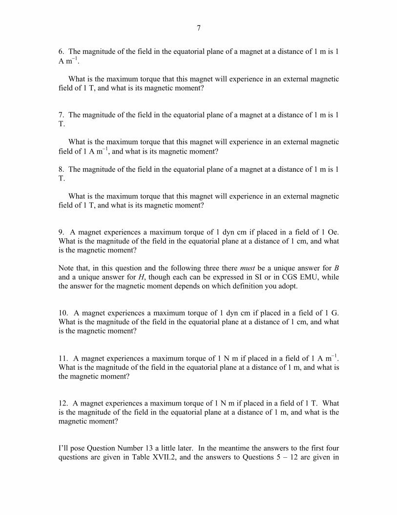
7

6. The magnitude of the field in the equatorial plane of a magnet at a distance of 1 m is 1 A m−1. What is the maximum torque that this magnet will experience in an external magnetic field of 1 T, and what is its magnetic moment? 7. The magnitude of the field in the equatorial plane of a magnet at a distance of 1 m is 1 T. What is the maximum torque that this magnet will experience in an external magnetic field of 1 A m−1, and what is its magnetic moment? 8. The magnitude of the field in the equatorial plane of a magnet at a distance of 1 m is 1 T. What is the maximum torque that this magnet will experience in an external magnetic field of 1 T, and what is its magnetic moment? 9. A magnet experiences a maximum torque of 1 dyn cm if placed in a field of 1 Oe. What is the magnitude of the field in the equatorial plane at a distance of 1 cm, and what is the magnetic moment? Note that, in this question and the following three there must be a unique answer for B and a unique answer for H, though each can be expressed in SI or in CGS EMU, while the answer for the magnetic moment depends on which definition you adopt. 10. A magnet experiences a maximum torque of 1 dyn cm if placed in a field of 1 G. What is the magnitude of the field in the equatorial plane at a distance of 1 cm, and what is the magnetic moment? 11. A magnet experiences a maximum torque of 1 N m if placed in a field of 1 A m−1. What is the magnitude of the field in the equatorial plane at a distance of 1 m, and what is the magnetic moment? 12. A magnet experiences a maximum torque of 1 N m if placed in a field of 1 T. What is the magnitude of the field in the equatorial plane at a distance of 1 m, and what is the magnetic moment? I’ll pose Question Number 13 a little later. In the meantime the answers to the first four questions are given in Table XVII.2, and the answers to Questions 5 – 12 are given in

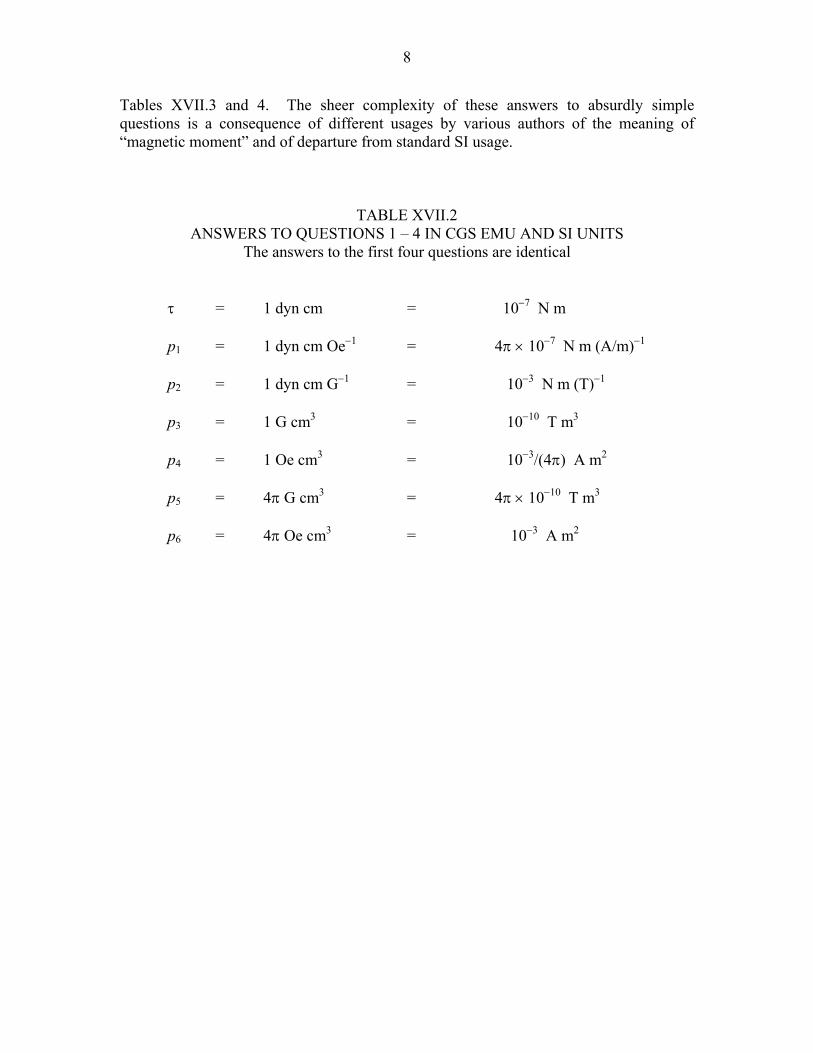
8

Tables XVII.3 and 4. The sheer complexity of these answers to absurdly simple questions is a consequence of different usages by various authors of the meaning of “magnetic moment” and of departure from standard SI usage.

TABLE XVII.2 ANSWERS TO QUESTIONS 1 – 4 IN CGS EMU AND SI UNITS

The answers to the first four questions are identical

τ = 1 dyn cm = 10−7 N m p1 = 1 dyn cm Oe−1 = 4π × 10−7 N m (A/m)−1

p2 = 1 dyn cm G−1 = 10−3 N m (T)−1 p3 = 1 G cm3 = 10−10 T m3 p4 = 1 Oe cm3 = 10−3/(4π) A m2 p5 = 4π G cm3 = 4π × 10−10 T m3 p6 = 4π Oe cm3 = 10−3 A m2

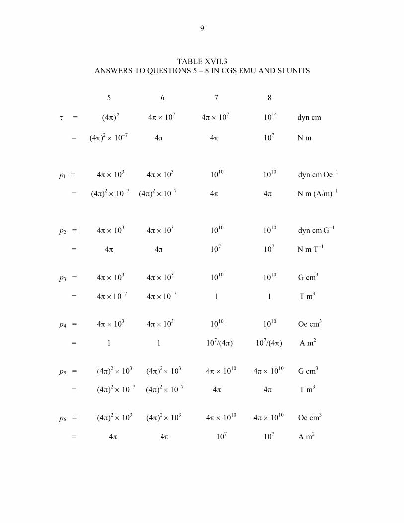
9

TABLE XVII.3

ANSWERS TO QUESTIONS 5 – 8 IN CGS EMU AND SI UNITS 5 6 7 8 τ = 2)4( π 4π × 107 4π × 107 1014 dyn cm = (4π)2 × 10−7 4π 4π 107 N m pl = 4π × 103 4π × 103 1010 1010 dyn cm Oe−1

= (4π)2 × 10−7 (4π)2 × 10−7 4π 4π N m (A/m)−1

p2 = 4π × 103 4π × 103 1010 1010 dyn cm G−1

= 4π 4π 107 107 N m T−1

p3 = 4π × 103 4π × 103 1010 1010 G cm3

= 4π × 10−7 4π × 10−7 1 1 T m3

p4 = 4π × 103 4π × 103 1010 1010 Oe cm3

= 1 1 107/(4π) 107/(4π) A m2

p5 = (4π)2 × 103 (4π)2 × 103 4π × 1010 4π × 1010 G cm3

= (4π)2 × 10−7 (4π)2 × 10−7 4π 4π T m3

p6 = (4π)2 × 103 (4π)2 × 103 4π × 1010 4π × 1010 Oe cm3

= 4π 4π 107 107 A m2

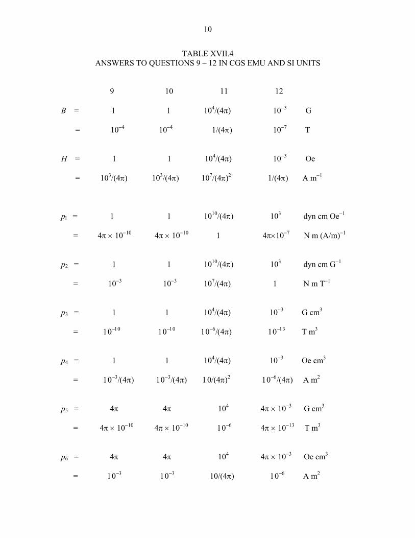
10

TABLE XVII.4 ANSWERS TO QUESTIONS 9 – 12 IN CGS EMU AND SI UNITS

9 10 11 12 B = 1 1 104/(4π) 10−3 G = 10−4 10−4 1/(4π) 10−7 T H = 1 1 104/(4π) 10−3 Oe = 103/(4π) 103/(4π) 107/(4π)2 1/(4π) A m−1

pl = 1 1 1010/(4π) 103 dyn cm Oe−1

= 4π × 10−10 4π × 10−10 1 4π×10−7 N m (A/m)−1

p2 = 1 1 1010/(4π) 103 dyn cm G−1

= 10−3 10−3 107/(4π) 1 N m T−1

p3 = 1 1 104/(4π) 10−3 G cm3

= 10−10 10−10 10−6/(4π) 10−13 T m3

p4 = 1 1 104/(4π) 10−3 Oe cm3

= 10−3/(4π) 10−3/(4π) 10/(4π)2 10−6/(4π) A m2

p5 = 4π 4π 104 4π × 10−3 G cm3

= 4π × 10−10 4π × 10−10 10−6 4π × 10−13 T m3

p6 = 4π 4π 104 4π × 10−3 Oe cm3

= 10−3 10−3 10/(4π) 10−6 A m2

11

The thirteenth and last of these questions is as follows: Assume that Earth is a sphere of radius 6.4 × 106 m = 6.4 × 108 cm, and that the surface field at the magnetic equator is

,Oe3.0mA/75orG,3.0T103 15 =π==×= −− HB what is the magnetic moment of Earth? It is hard to imagine a more straightforward question, yet it would be hard to find two people who would give the same answer. The SI answer (which, to me, is the only answer) is

227

536

0

3

30 1086.7

104103)104.6(44,

4×=

×π××××π

=µπ

=π

µ= −

−BrprpB ∴ N m T−1.

This result correctly predicts that, if Earth were placed in an external field of 1 T, it would experience a maximum torque of 7.86 × 1022 N m, and this is the normal meaning of what is meant by magnetic moment. A calculation in GCS might proceed thus:

.cmG1086.73.0)104.6(, 3253833 ×=××=== Brp

rpB ∴

Is this the same result as was obtained from the SI calculation? We can use the conversions 1 G = 10−4 T and 1 cm3 = 10−6 m3, and we obtain p = 7.86 × 1015 T m3. We arrive at a number that not only differs from the SI calculation by 107, but is expressed in quite different, dimensionally dissimilar, units. Perhaps the CGS calculation should be

.cmOe1086.73.0)104.6(, 3253833 ×=××=== Hrp

rpH ∴

Now 1 Oe = 1000/(4π) A m−1 and 1 cm3 = 10−6 m3, and we obtain p = 6.26 × 1021 A m2 This time we arrive at SI units that are dimensionally similar to N m T−1, and which are perfectly correct SI units, but the magnetic moment is smaller than correctly predicted by the SI calculation by a factor of 12.6. Yet again, we might do what appears to be frequently done by planetary scientists, and we can multiply the surface field in T by the cube of the radius in m to obtain

12

p = 7.86 × 1015 T m3. This arrives at the same result as one of the CGS calculations, but, whatever it is, it is not the magnetic moment in the sense of the greatest torque in a unit field. The quantity so obtained appears to be nothing more that the product of the surface equatorial field and the cube of the radius, and as such would appear to be a purposeless and meaningless calculation. It would be a good deal more meaningful merely to multiply the surface value of H by 3. This in fact would give (correctly) the dipole moment divided by the volume of Earth, and hence it would be the average magnetization of Earth – a very meaningful quantity, which would be useful in comparing the magnetic properties of Earth with those of the other planets. 17.7 Additional Remarks The units erg G−1 or J T−1 are frequently encountered for magnetic moment. These may be dimensionally correct, although ergs and joules (units of energy) are not quite the same things as dyn cm or N m as units of torque. It could be argued that magnetic moment could be defined from the expression −p.B for the potential energy of a magnet in a magnetic field. But the correct expression is actually constant − p.B, the constant being zero only if you specify that the energy is taken to be zero when the magnetic moment and field vectors are perpendicular to each other. This seems merely to add yet further complications to what should be, but unfortunately is not, a concept of the utmost simplicity. Nevertheless the use of ergs or joules rather than dyn cm or N m is not uncommon, and nuclear and particle physicists commonly convert joules to MeV. Magnetic moments of atomic nuclei are commonly quoted in nuclear magnetons, where a nuclear magneton is

)2/( pmeh and has the value 3.15 × 10−4 MeV T−1. While one is never likely to want to express the magnetic moment of the planet Uranus in nuclear magetons, it is sobering to attempt to do so, given that the magnetic moment of Uranus is quoted as 0.42 Oe km−1. While on the subject of Uranus, I have seen it stated that the magnetic quadrupole of Uranus is or the same order of magnitude as its magnetic dipole moment – though, since these are dimensionally dissimilar quantities, such a statement conveys no meaning. Another exercise to illustrate the points I have been trying to make is as follows. From four published papers I find the following. The magnetic moment of Mercury is 1.2 × 1019 A m2 in one paper, and 300 nT RM

3 in another. The magnetic moment of Uranus is 4.2 × 1012 Oe km3 in one paper, and 0.23 G RU

3 in another. The radii of Mercury and Uranus are, respectively, 2.49 × 106 m and 2.63 × 107 m. Calculate the ratio of the magnetic moment of Uranus to that of Mercury. If you are by now completely confused, you are not alone.

13

17.8 Conclusion Readers will by now probably be bewildered at the complexities described in this chapter. After all, there could scarcely be a simpler notion than that of the torque experienced by a magnet in a magnetic field, and there would seem to be no need for all of these complicated variations. You are right – there is no such need. All that need be known is summarized in Sections 17.2 and 17.3. The difficulty arises because authors of scientific papers are using almost all possible variations of what they think is meant by magnetic moment, and this has led to a thoroughly chaotic situation. All I can do is to hope that readers of these notes will be encouraged to use only the standard SI definition and units for magnetic moment, and to be aware of the enormous complications arising when they depart from these.

1

CHAPTER 10

ELECTROCHEMISTRY For a long time I have resisted writing a chapter on electrochemistry in these notes on electricity and magnetism. The reason for this, quite frankly, is that I am not a chemist, I know relatively little about the subject, and I am not really qualified to write on it. However, a set of notes on electricity and magnetism with no mention at all of this huge topic is not very satisfactory, so I should perhaps attempt a little. I shall do little, however, other than merely introduce and define some words. We can perhaps think of two sorts of cell with rather opposite purposes. In an electrolytic cell, we pass an electric current through a conducting liquid through two electrodes, which may be of the same or of different metals. The object may simply be to see what happens (i.e. scientific research); or it may be to deposit a metal from a salt in the electrolytic solution on to one of the electrodes, as, for example, in silver plating, or in the industrial manufacture of aluminium; or it may be to break up the electrolyte into its constituent elements, as, for example, in a classroom demonstration that water consists of two parts of hydrogen to one of oxygen. The process is called electrolysis; the Greek etymology of the word electrolysis suggests "loosening" by electricity. The other sort is what we commonly call a "battery", such as a flashlight battery or a car battery. In a “battery”, we have an electrolyte and two metal poles (generally of different metals, or perhaps a metal and carbon). Because of chemical reactions inside the battery, there exists a small potential difference (usually about one or two volts) across the poles, and when the "battery" is connected to an external circuit, we can extract a continuous current from the battery. Strictly, we should call it a “cell” rather than a “battery”. A “battery” is a battery of several cells in series. Usually a flashlight holds a battery of two or three cells. A car battery is genuinely a battery of several connected cells and can correctly be called a battery. Unfortunately in common parlance we often refer to a single cell as a “battery”. In order to distinguish a cell in this sense from what I have called an "electrolytic cell", I shall refer to a cell from which we hope to extract a current as an "electrical cell". I hope these opposite terms "electrolytic cell" and "electric cell" do not prove too confusing. If they do, I'd be glad of suggestions. One suggestion that I have heard is to call an electric cell a "galvanic cell". Another is a "voltaic cell". In an electrolytic cell, the positive electrode is called the anode, from a Greek derivation suggesting "up". The negative electrode is the cathode, from a Greek derivation suggesting "down". In the electrolyte, current is carried by positive ions and negative ions. The positive ions, which move toward the cathode, are called cations, and the negative ions, which move towards the anode, are called anions. Do you find it confusing that the positive electrode is the anode, but the positive ion is the cation? And that the negative electrode is the cathode, but the negative ion is the anion? If you do, you are not alone. I find them confusing. Solution: I suggest that you call the positive electrode the positive electrode; the negative electrode the negative electrode; the positive ion the positive ion; and the negative ion the negative ion. That way there is no likelihood of your being misunderstood.

2

Now, when we come to electrical cells, it may be that the roles of the electrodes are reversed. What was a positive electrode in an electrolytic cell may be the negative side of an electrical cell. What are we going to call them? I suggest that, when we are talking about electrical cells we do not use the word "electrode" at all. We shall refer to the positive pole and the negative pole of an electrical cell. Electrolysis of Water I vaguely remember my first impressions of what is supposed to happen when two platinum electrodes are dipped into water and a current is passed into the water. My guess is that, if the water were very pure water (which is quite difficult to come by) very little would happen. Pure water has very few ions in it (we'll discuss just how many a little later) and its electrical conductivity is quite small – about 5.5 % 10−6 S m−1. However, real water is not pure; it usually has enough impurities in it to supply plenty of ions and to make it a good conductor (and hence a danger in the presence of high-voltage equipment). My early impression (not quite accurate) of what happens when an electric current passes through water was something like this. Water contains, in addition to billions of molecules of H2O, a few ions formed through the partial dissociation of H2O: H2O ↔ H+ + OH−

The hydrogen ions, which are the cations positive ions, move one way, and the hydroxyl ions, which are the negative ions, move the other way. Well, I'm happy to believe in the existence (if not, maybe, the movement) of the hydroxyl ions, but not about the H+ ions, which are bare protons with an enormous electrical field. I don't think bare protons exist in any liquid electrolyte, let alone water. I think the reaction is more like

H2O + H2O ↔ H3O+ + OH−

The positive ion is actually a hydrated proton, also known as “hydronium”. My other problem is that I have difficulty in imagining these great clumsy ions trying to barge their way (the H3O+ ions one way, and the hydroxyl ions the other way) through the milling crowd of H2O molecules. If you imagine the positive electrode to be at the left and the negative electrode at the right, so that the electric field is from left to right, I think what happens when an ion bumps into a neutral water molecule is something like this:

H3O+ + H2O → H2O + H3O+ and H2O + OH− → OH− + H2O In either case, a proton is swapped between the jostling bodies, and so the proton moves from left to right.

3

Be that as it may, the following reactions occur at the negative electrode A fresh supply of hydroxyl ions is continuously being created while hydrogen molecules are being released in gaseous form

2H2O + 2e− → 2OH− + H2 ↑

Also, arriving hydrated protons are neutralized:

2H3O+ + 2e− → 2H2O + H2 ↑ At the positive electrode, a fresh supply of hydrated protons is continuously being created while oxygen molecules are being released in gaseous form. This happens by electrons from H2O molecules being transferred to the positive electrode, in several stages, but with net result:

6H2O − 4e− → 4H3O+ + O2 ↑

In addition, arriving hydroxyl ions are neutralized: 4OH− − 4e− → 2H2O + O2 ↑ The whole process might seem a bit complicated, but, since we start off in water with twice as many hydrogen atoms as oxygen atoms, naturally the electrolysis results in hydrogen molecules being produced at twice the rate of oxygen molecules. Furthermore, the net result is the same as if we had supposed that there were indeed OH− and H+ ions moving through the water as in the simplest model. One last point before we leave water. I mentioned that the electrical conductivity of pure water is very small, and the number of ions is very small, so that probably not much would happen if you tried to electrolyse pure water. Real water is rarely pure and it has enough impurity ions in it to allow an electrolysis experiment to proceed smoothly. In pure water at room temperature there are about 10−7 moles of hydrogen ions (hydrated protons) and a similar number of hydroxyl ions per litre. In SI units, that is also 10−7 kmole per m3. If you add a little bit of acid, you of course very much increase the number of hydrogen ions, and correspondingly the number of hydroxyl ions drops. (Don’t worry – the solution remains electrically neutral! If, for example, the acid is HCl, there will be lots of Cl− ions.) The number of hydrogen ions per litre might be, for example, 10−5 mole per litre, or kmole per m3. If you add a little alkali, you increase the number of hydroxyl ions and correspondingly decrease the number of hydrogen atoms, perhaps to 10−9 mole per litre, or kmole per m3. (Don’t worry – the solution remains electrically neutral! If, for example, the alkali is NaOH, there will be lots of Na+ ions.) The absolute value of that exponent (7 for the neutral solution, 5 for the acidic solution, 9 for the alkaline solution) is called the pH. I think the symbol p was originally chosen from the German Potenz, or potential or power. The pH is commonly used to describe the acidity or alkalinity of a

4

solution. It is 7 for a neutral solution, less than 7 for an acidic solution, and greater than 7 for an alkaline solution. Actually, pH is just a rather rough indication of acidity, and there is often not much value in quoting a pH value to a large number of significant figures. For example, in hot water, more water molecules are dissociated, so there are more hydrogen ions (and of course more hydroxyl ions) so the pH value would nominally go down – though the hot water is no more acidic that it was when it was cold. Electrolysis of silver nitrate. There are countless examples of electrolysis that could be told in an encyclopaedia devoted to the subject, many of which are industrial applications. But I don’t want to (indeed cannot) write a chemistry book. And indeed all that I need here is one example that is sufficient to introduce some scientific words. I choose the electrolysis of silver nitrate partly because it is simple; partly because at one time the practical definition of the amp was based on the rate of deposition of silver from silver nitrate solution; partly because it enables me to mention Faraday's law and the definition of the faraday, and even to mention Avogadro's number; partly because the electrolysis of silver nitrate can be used for very precise measurement of electric current, and partly because it is used in practice for silver plating. The stoichiometric chemical formula for silver nitrate is AgNO3, though in fact, both in the crystalline state and in solution, it consists of Ag+ and NO3

+ ions. During electrolysis of silver nitrate solution with silver electrodes, silver, of course, is deposited on the negative electrode. Oxygen is given off at the positive electrode. I mention this, because at one time (apart from the obvious practical use in silver plating), this was used as the practical definition of the unit the amp, or ampère. Indeed an “international amp” was that steady current which would deposit silver at a rate of 0.001118 grams of silver per second from a solution of silver nitrate. (This value is very close indeed to, though a tiny bit less than, the SI definition of the amp described in Chapter 6.) Oxygen is given off at the positive electrode. Faraday measured the mass of many metals deposited from various electrolytes, and he enunciated what is now known as Faraday's Law of Electrolysis. In simple terms, and without using phrases that are more familiar to chemists than to physicists, Faraday's law could be stated as:

m It∝

µv

That is to say, the mass m of a metal deposited on the cathode during electrolysis is proportional to the total quantity of electricity passed (that is It, where I is the current and t is the time), to the molar mass (i.e. the mass of a mole of the metal, popularly known as the "atomic weight") and inversely proportional to the “valence” or “valency” v, which is just the charge on the ion. For example aluminium has a valence of 3. Its ion has a charge of plus 3 electronic charges, and consequently it needs three times the amount of electricity to deposit a mole of Al than to deposit, say, a mole of univalent Ag. The molar mass of a metal divided by its valence is called the electrochemical equivalent of the metal. It is the mass of metal that would be deposited by a

5

coulomb of electricity. ( .Itm

=µv

) A silver nitrate electrolytic cell is in fact a very suitable

instrument for the highly precise measurement of electric current. In this connection it is called a voltameter, though I suppose “ammeter” would really be a better name! So, how much electricity is required to deposit a mole of charge? (That is to say a mole of the metal ions times the charge on each.) The amount of electricity required to deposit a mole of charge (e.g. 108 grams of Ag, or 27 ÷ 3 = 9 grams of Al) from solution is called a faraday. It is about 96,485 C, which is the charge of a mole (Avogadro's number) of electrons. This is worth knowing, for a good examination question for physics students might be "How is Avogadro's number determined?" This is obviously a very important thing for a physicist to know, but a physics student with only a modest background in chemistry might not immediately think of the answer, which is: by measuring the size of the faraday by measuring the mass of silver deposited from silver nitrate solution. (Of course you have to use the SI definition of the amp for this – it wouldn’t do to use the definition of the “international amp”!)

ELECTRICITY AND MAGNETISM Chapter 1. Electric Fields ...

Documents

Transcript of ELECTRICITY AND MAGNETISM Chapter 1. Electric Fields ...