Repeat-track SAS interferometry : feasibility studyR. Bellec, M. Legris, A. Khenchaf

Laboratoire E3I2 EA3876Ecole Nationale Superieure des Ingenieursdes Etudes et Techniques de l’Armement

2, rue Francois Verny, 29806 Brest Cedex 9, FranceEmail: {bellecro, legrismi, khenchal}@ensieta.fr

M. Amate, A. HetetGroupe d’Etudes Sous-Marines de l’Atlantique

DGA/DET/GESMABP 42 - 29240 Brest Armees, France

Email: {maud.amate, alain.hetet}@dga.defense.gouv.fr

Abstract— Repeat track interferometry is a commonly usedtechnology in Radar. It permits to obtain topography and eleva-tion variation of ground. This technology is not used with sonarsystem, even though this configuration could provide interestingapplications for underwater environnement knowledge. Thispaper presents a study on repeat-track interferometry feasibilitywith sonar system, and especially for synthetic aperture sonar(SAS). We shortly expose the SAS and interferometry principlein the first part. Then we present the multi-track interferometryand discuss on limitation. In a third part, experimental resultsbased on data acquired with the experimental low frequencySAS (LFSAS) of GESMA (France), are detailed and we exposemethods to circumvent problems induced by repeat-track inter-ferometry. Finally we discuss on future strategies to improve theencouraging results we obtained.

I. INTRODUCTION

Repeat-track interferometry is a commonly used technol-ogy in SAR (Synthetic Aperture Radar) for many years.From two tracks, done at different dates, an interferometricimage is computed to evaluate the ground topography orthe elevation variation (differential interferometry). In SASdevelopment (Synthetic Aperture Sonar), some InSAS (Inter-ferometric SAS) configurations have been studied and carriedout. These InSAS projects are all simple-track SAS using twoantennas, which is a costly system. Track-repetition techniquehas not been studied yet according to our knowledge. Suchconfiguration is known to be problematic to develop due tothe lack of medium coherency and precision of navigation.Nevertheless, as repeat-track interferometry has many potentialapplications, we have decided to investigate more thoroughlythe limitations of this configuration.

The paper presents the multi-track interferometry includingunderwater imaging specificities and examines the theoreticaland practical limitations of such configuration. In this study,we focus the theoretical studies on four factors of influence:sliding-footprint due to errors on image registration, angularde-correlation from differences in sensors locations, signal tonoise ratio and medium variability. We then present someresults obtained from data acquired during a SAS trial jointlycarried out by GESMA (France) and TNO, Defense, Secu-rity and Safety (The Netherlands) on September 2002, nearBrest. Finally, the paper presents a discussion on the possibleapplications of such configurations.

II. BACKGROUND

A. Synthetic Aperture Sonar

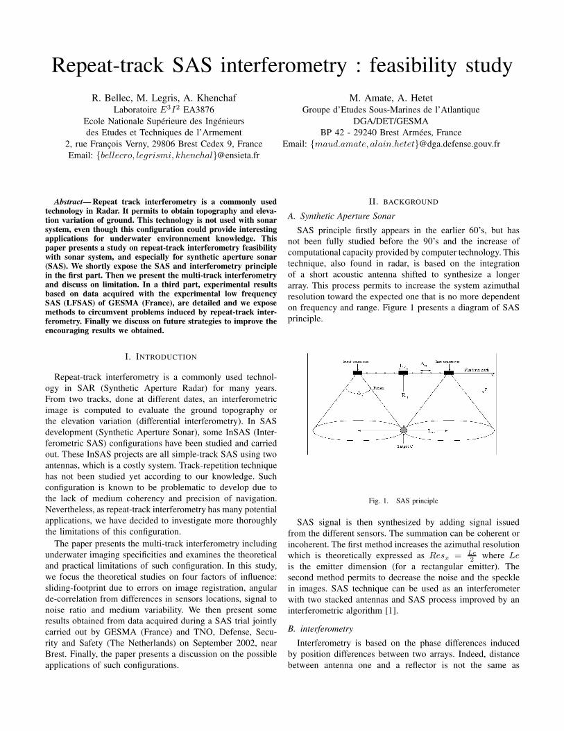
SAS principle firstly appears in the earlier 60’s, but hasnot been fully studied before the 90’s and the increase ofcomputational capacity provided by computer technology. Thistechnique, also found in radar, is based on the integrationof a short acoustic antenna shifted to synthesize a longerarray. This process permits to increase the system azimuthalresolution toward the expected one that is no more dependenton frequency and range. Figure 1 presents a diagram of SASprinciple.

Fig. 1. SAS principle

SAS signal is then synthesized by adding signal issuedfrom the different sensors. The summation can be coherent orincoherent. The first method increases the azimuthal resolutionwhich is theoretically expressed as Resx = Le

2 where Leis the emitter dimension (for a rectangular emitter). Thesecond method permits to decrease the noise and the specklein images. SAS technique can be used as an interferometerwith two stacked antennas and SAS process improved by aninterferometric algorithm [1].

B. interferometry

Interferometry is based on the phase differences inducedby position differences between two arrays. Indeed, distancebetween antenna one and a reflector is not the same as

distance between antenna two and this reflector (cf fig.2). Thephase difference between two signals is only due to geometrydifferences because the proper phase of the reflectors is seenas the same by both antennas (limitation are exposed in nextpart). Phase difference is computed by the product S1∗S2 (with(.) represents complex conjugate of (.)) to which we add thegroup phase difference which is equal to entire part of cyclethat separate the two signal S1 and S2. Phase difference andaltitude of a particular reflector is expressed as following :

∆φ =2πλd cos(α + ψ) (1)

h = H −R0 cos(α) (2)

Fig. 2. Interferometer geometry

III. MULTI-TRACK CONFIGURATION

Interferometry can also be processed from two tracks ac-quired at different dates but in similar position with respectto the scene. This configuration is daily used in radar [2]and more particularly with satellite radar because trajectoryis well controlled. An other point specific to the SAS or SARprocess is that antennas used to compose the interferometerare not constant in their geometry. This is more problematicwith sonar because trajectories are not controlled as well asin radar, antenna distorsion are known with lower accuracy.Sonar multi-track seems also more difficult to design becausethe medium is not as stable as atmosphere is for radar.

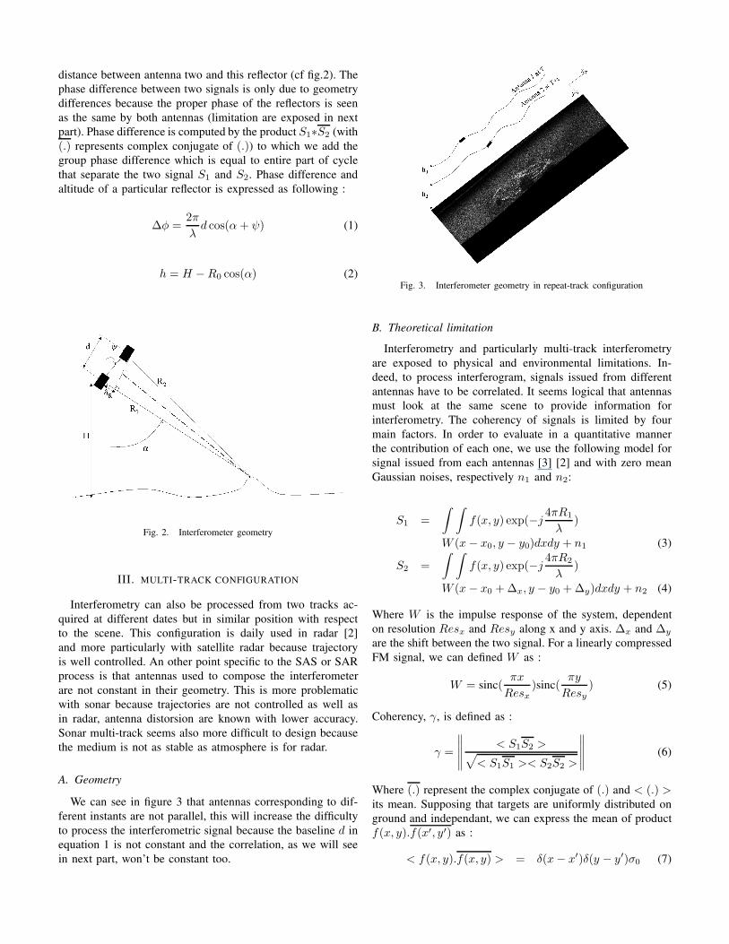
A. Geometry

We can see in figure 3 that antennas corresponding to dif-ferent instants are not parallel, this will increase the difficultyto process the interferometric signal because the baseline d inequation 1 is not constant and the correlation, as we will seein next part, won’t be constant too.

Fig. 3. Interferometer geometry in repeat-track configuration

B. Theoretical limitation

Interferometry and particularly multi-track interferometryare exposed to physical and environmental limitations. In-deed, to process interferogram, signals issued from differentantennas have to be correlated. It seems logical that antennasmust look at the same scene to provide information forinterferometry. The coherency of signals is limited by fourmain factors. In order to evaluate in a quantitative mannerthe contribution of each one, we use the following model forsignal issued from each antennas [3] [2] and with zero meanGaussian noises, respectively n1 and n2:

S1 =∫ ∫

f(x, y) exp(−j 4πR1

λ)

W (x− x0, y − y0)dxdy + n1 (3)

S2 =∫ ∫

f(x, y) exp(−j 4πR2

λ)

W (x− x0 + ∆x, y − y0 + ∆y)dxdy + n2 (4)

Where W is the impulse response of the system, dependenton resolution Resx and Resy along x and y axis. ∆x and ∆y

are the shift between the two signal. For a linearly compressedFM signal, we can defined W as :

W = sinc(πx

Resx)sinc(

πy

Resy) (5)

Coherency, γ, is defined as :

γ =

∥∥∥∥∥< S1S2 >√

< S1S1 >< S2S2 >

∥∥∥∥∥ (6)

Where (.) represent the complex conjugate of (.) and < (.) >its mean. Supposing that targets are uniformly distributed onground and independant, we can express the mean of productf(x, y).f(x′, y′) as :

< f(x, y).f(x, y) > = δ(x− x′)δ(y − y′)σ0 (7)

If we consider no miss-registration along x axis, i.e. ∆x = 0,that leads to :

< S1.S2 > = σ0ResxResy exp(−j 4π(R1 −R2)λ

)β

(8)

Fig. 4. Simplified geometry of interferometric system

Considering the simplified geometry presented on fig 4,and after first order Taylor expansion, R1 − R2 can beapproximated to yd

ρ , it comes:

β = (1 − 2dResy

λρ) exp(−j 2πd∆y

λρ)

sinc(π∆y

Resy(1 − 2dResy

λρ)) (9)

If we consider that noise have the same variance, σn, forboth acquisitions, that lead to :

< S1.S1 > = < S2.S2 >= σ0ResxResy + σ2n (10)

Correlation is expressed :

γ =σ0ResxResy

σ0ResxResy + σ2n

|β| (11)

The correlation between the images with independent noiseof same variance can be expressed as a function of SNR =σ0ResxResy/σ

2n (signal to noise ratio) and a geometric influ-

ence |β|:γSNR =

11 + SNR−1

Geometric parameters that influence the correlation qualitycan be decomposed in two components. Angular differencesin the observation of the scene that are induced by the baselinedimensions are expressed as :

γbase = 1 − 2dResy

λρ

This expression can also be deduced by the VanCittert-Zerniketheorem. We can notice that correlation depends on ρ, theless the view angle difference is the more data are correlated.This dependence on ρ is unfortunately attenuated by SNR thatincrease as ρ does.

The second term of |β| describes foot-print shape dif-ferences and images miss-registration influence. This de-correlation phenomenon, noted γsfp (sfp for sliding foot-print)is expressed as :

γsfp = sinc(π∆y

Resy(1 − 2dResy

λρ))

A last factor is the environmental factor that is more specificto the multi-track interferometer, noted γtemp. The coherenceshould not be kept between the two tracks because medium(water or ocean for instance) or the scene might have changedin the time that separate the two tracks. Sand dune or objectlaid on ground may have moved, water temperature or salinitymay have evolved during the elapsed time and any otherphenomenon could influence the correlation between signals.Influence of such temporal environment variability has beenmodeled by Zebker [4] as:

γtemp = exp{−12(4πλ

2

(σ2ysin

2α+ σ2zcos

2α))}where σy and σz represent the standard deviation of themean random shift, physically induced by error on celerityestimation and reflector migration, respectively in range andin altitude. Unfortunately, we don’t have any data or modelto evaluate this expression in our experimental conditions.Literature does not provide any information exploitable forthe estimation of γtemp for scale and time periods that we areconcerned on.

The global correlation could be expressed as the product ofthe de-correlation induced by the previously quoted causes.

γ = γSNRγbaseγsfpγvariability

This de-correlation induces errors in phase differences estima-tion and involves a more problematic unwrapping process.

IV. REAL-DATA EXPLOITATION

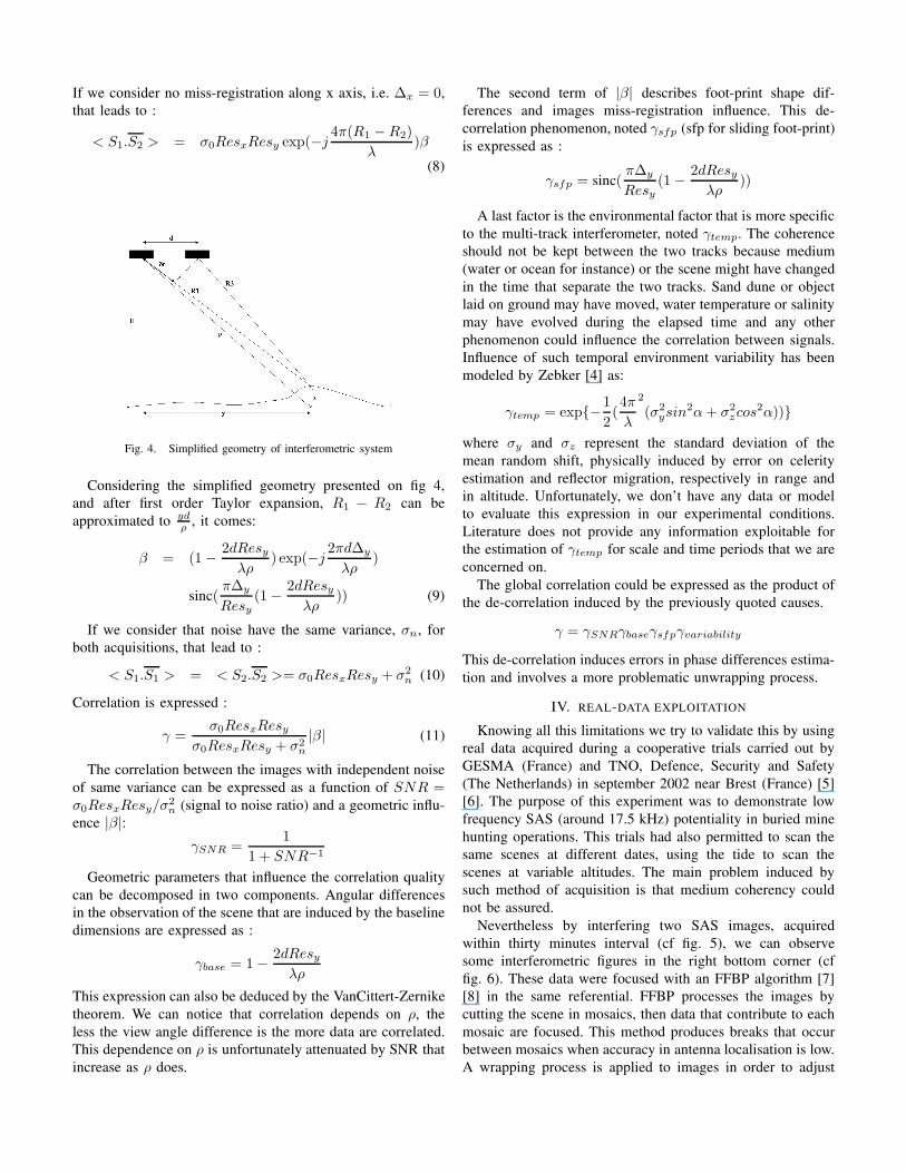
Knowing all this limitations we try to validate this by usingreal data acquired during a cooperative trials carried out byGESMA (France) and TNO, Defence, Security and Safety(The Netherlands) in september 2002 near Brest (France) [5][6]. The purpose of this experiment was to demonstrate lowfrequency SAS (around 17.5 kHz) potentiality in buried minehunting operations. This trials had also permitted to scan thesame scenes at different dates, using the tide to scan thescenes at variable altitudes. The main problem induced bysuch method of acquisition is that medium coherency couldnot be assured.

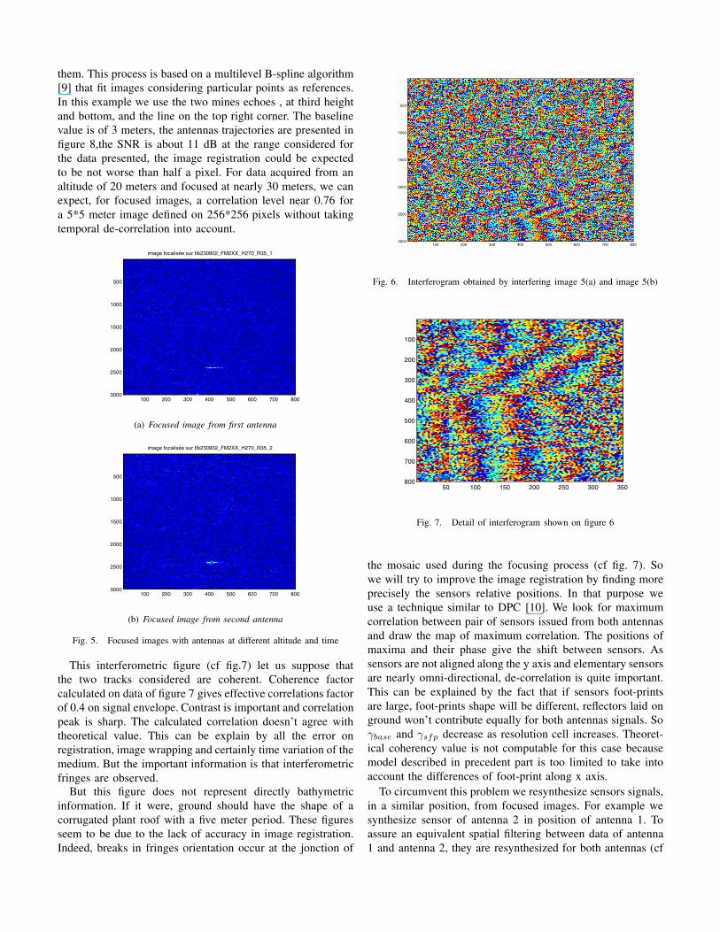
Nevertheless by interfering two SAS images, acquiredwithin thirty minutes interval (cf fig. 5), we can observesome interferometric figures in the right bottom corner (cffig. 6). These data were focused with an FFBP algorithm [7][8] in the same referential. FFBP processes the images bycutting the scene in mosaics, then data that contribute to eachmosaic are focused. This method produces breaks that occurbetween mosaics when accuracy in antenna localisation is low.A wrapping process is applied to images in order to adjust

them. This process is based on a multilevel B-spline algorithm[9] that fit images considering particular points as references.In this example we use the two mines echoes , at third heightand bottom, and the line on the top right corner. The baselinevalue is of 3 meters, the antennas trajectories are presented infigure 8,the SNR is about 11 dB at the range considered forthe data presented, the image registration could be expectedto be not worse than half a pixel. For data acquired from analtitude of 20 meters and focused at nearly 30 meters, we canexpect, for focused images, a correlation level near 0.76 fora 5*5 meter image defined on 256*256 pixels without takingtemporal de-correlation into account.

image focalisée sur tlb230902_FM2XX_H270_R35_1

100 200 300 400 500 600 700 800

500

1000

1500

2000

2500

3000

(a) Focused image from first antenna

image focalisée sur tlb230902_FM2XX_H270_R35_2

100 200 300 400 500 600 700 800

500

1000

1500

2000

2500

3000

(b) Focused image from second antenna

Fig. 5. Focused images with antennas at different altitude and time

This interferometric figure (cf fig.7) let us suppose thatthe two tracks considered are coherent. Coherence factorcalculated on data of figure 7 gives effective correlations factorof 0.4 on signal envelope. Contrast is important and correlationpeak is sharp. The calculated correlation doesn’t agree withtheoretical value. This can be explain by all the error onregistration, image wrapping and certainly time variation of themedium. But the important information is that interferometricfringes are observed.

But this figure does not represent directly bathymetricinformation. If it were, ground should have the shape of acorrugated plant roof with a five meter period. These figuresseem to be due to the lack of accuracy in image registration.Indeed, breaks in fringes orientation occur at the jonction of

100 200 300 400 500 600 700 800

500

1000

1500

2000

2500

3000

Fig. 6. Interferogram obtained by interfering image 5(a) and image 5(b)

50 100 150 200 250 300 350

100

200

300

400

500

600

700

800

Fig. 7. Detail of interferogram shown on figure 6

the mosaic used during the focusing process (cf fig. 7). Sowe will try to improve the image registration by finding moreprecisely the sensors relative positions. In that purpose weuse a technique similar to DPC [10]. We look for maximumcorrelation between pair of sensors issued from both antennasand draw the map of maximum correlation. The positions ofmaxima and their phase give the shift between sensors. Assensors are not aligned along the y axis and elementary sensorsare nearly omni-directional, de-correlation is quite important.This can be explained by the fact that if sensors foot-printsare large, foot-prints shape will be different, reflectors laid onground won’t contribute equally for both antennas signals. Soγbase and γsfp decrease as resolution cell increases. Theoret-ical coherency value is not computable for this case becausemodel described in precedent part is too limited to take intoaccount the differences of foot-print along x axis.

To circumvent this problem we resynthesize sensors signals,in a similar position, from focused images. For example wesynthesize sensor of antenna 2 in position of antenna 1. Toassure an equivalent spatial filtering between data of antenna1 and antenna 2, they are resynthesized for both antennas (cf

−20

−18

−16

−14

−10

12

3

−1

−0.8

−0.6

−0.4

−0.2

0

0.2

0.4

azimuth (m)

antennas trajectory

range (m)

altit

ude

(m)

antenna 1antenna 2

Fig. 8. Trajectory of two antennas processed with 30 minutes elapsed timebetween acquisition, referential is attached to antenna 1

illustration 12). The synthesis is processed with a temporalalgorithm, summarized with equation 12.

S′i(t) =

∫ θimage2

− θimage2

A(θ, t)W (θ) dθ (12)

Where θimage is the image visibility field of the sensor iat date t. W is the impulse response of the system, i.e. theemission/reception directivity diagram. Parameter A(θ, t) isthe complex signal of the image.

We so have signals issued from virtually same positionantennas at different date. This leads to signal represented onfigure 9. We observed that signals are quite similar includingclutter areas. This is a sign of coherence between data.Interferences produced with the two sensors data series provideus an image (cf fig. 10) that presents a slowly shifting phase,interpretable as a residual angle between the two antennastrajectory. Coherency computed with these synthesized sensordata gave us bad results. These results can be explained bythe phase shifting. Correlation found on reduced window (inthat case 32 points large) which assure a quasi constant phase,gives us better results. The figure 11 was made by multiplyingthe different results obtained with the correlation on reducedwindows. We can observe a diagonal which allows us to hopeto find the fine miss-registration between sensors. Unfortu-nately the correlation absolute values are lower than thoseexpected and the information in cross-correlation diagram,figure 11, is not good enough to allow efficient exploitation. Toimprove this correlation factor and to obtain a better resolutionin correlation diagonal, we tried to make correlation on largerwindows. To permit the correlation on larger window, we cantry to find the phase rotation in this image, indeed this shiftin phase can be expressed as a phase term to add to the signalof sensors:

S′1 = S exp(jω) (13)

S′2 = S exp(j(aω + b)) (14)

real raw data antenna 1

50 100 150 200

100

200

300

synthetic raw data antenna 1

50 100 150 200

100

200

300

(a) Antenna 1 signals

real raw data antenna 2

50 100 150 200

100

200

300

synthetic raw data antenna 2

50 100 150 200

100

200

300

(b) Antenna 2 signals

Fig. 9. Original signal S1 and S2 and re-synthesized signals S′1 et S′

2

where a is a dilation factor due to geometrical differencesand error in sound celerity estimation between the two tracksand b is due toW translation between the two positions. Theseterms, a and b, can be found by unwrapping the phase diagramand obtaining the local phase gradient. This unwrapping iscomputed by a previous filtering of phase diagram inspiredfrom [1] and expressed as :

∆φ(l, k) = arctan[

1KL

∑n

∑m w2�{Sl−m,k−n}∑

n

∑m w2�{Sl−m,k−n}

](15)

Where w is a weighting window chosen as Hanning, Hammingor Blackman centered on pixel of interest.It also should be awindow deduce from the auto-correlation of the interferogramto respect the coherency lenght of the signal. The unwrappingalgorithm is a 2D process which takes residues into account inorder to avoid aberrant points that appear with noisy data [3].This unwrapping gives us parameters to correct the dilationand sub-pixel translation between the two images. Consistentresults have not be reached yet because of unwrapping diffi-culty due to poor quality of the phase.

V. DISCUSSION

This technique could provide a method to improve theantennas trajectory estimation. Indeed, trajectory estimationis actually done by DPC algorithm which involves a drift

synthetized data interferogram

50 100 150 200

50

100

150

200

250

300

350

Fig. 10. Interferogram obtained with re-synthesized antennas signals

50 100 150 200 250 300 350

50

100

150

200

250

300

350

Fig. 11. Sensors cross coherency, coherency is computed on 32*32 windows

in trajectory estimation. DPC/INS fusion permits to solvepartially this problem, but correction of the drift is currentlyfar from perfection. Using the mutual information of twoantennas could provide us a mean to reduce the number ofdegrees of freedom of the system by constraining the relativesensors location. Information on errors between sensors ofboth antennas can be evaluated by using a third virtualtrajectory, chosen straight and linearly spaced sensors. As wecan see on illustration 12, we can measure the errors betweentwo series of data and deduce from this deformation the miss-registration. In operational conditions it could allow to havebetter focalisation on area where suspect objects were detected.

An other interest is to have, with such system, an oppor-tunity interferometer that could permit to obtain bathymetricinformation for area of interest. This bathymetric informationcould provide a way to improve the DPC algorithm byavoiding the flat-ground hypothesis usually done. However,this configuration has to be studied specifically because datafor the moment, don’t seem to be exploitable for an accuratebathymetry evaluation.

Fig. 12. Illustration of estimation of mutual miss-registry between twoantennas

VI. CONCLUSION

In this paper, we presented a study on multi-track inter-ferometry with SAS systems. This study shows limitationinvolved by interferometric system, this model had to bedeveloped to take into account the miss-registration of datain azimuth to evaluate the de-correlation induced by sensorwith large beamform diagram, i.e. low azimuthal resolution,used in low frequency SAS. Improving this model couldalso offer an opportunity to evaluate medium variability bycomparing measured coherence toward theoretical one. Aninteresting result is that interferogram can be processed andgives interference figure from two antennas that acquired dataat different date, in our example half an hour, other set ofdata were tested and gave similar results with elapsed time ofabout one hour. Coherence seems to decrease quickly but co-herency peak is still observable, but the main problem to haveexploitable interferometry data is the sensors path evaluation.While reversing the problem, repeat-track configuration couldalso help to evaluate the antennas trajectories.

REFERENCES

[1] Y. Perrot, “Imagerie tridimensionelle haute resolution du fond sous-marin par le traitement sonar interferometrique a ouverture synthetique,”Ph.D. dissertation, Universite de bretagne occidentale, UBO, 2001.

[2] E. Trouve, “Imagerie interferentielle en radar a ouverture synthetique,”Ph.D. dissertation, ENST-DRET, juillet 1996.

[3] F. K. Li and R. Goldstein, “Studies of multibaseline spaceborne interfer-ometric synthetic aperture radar,” IEEE transaction on Geoscience andRemote Sensing, vol. Vol. 28, pp. pp: 88–97, 1990.

[4] H. Zebker, C. Werner, P. Rosen, and S. Hensley, “Accuracy of topo-graphic maps derived from ERS-1 interferometric radar,” IEEE trans-action on Geoscience and Remote Sensing, vol. Vol. 32, pp. pp: 823–836,1994.

[5] A.Hetet, M. Amate, B. Zerr, M. Legris, R. Bellec, J. Sabel, and J. Groen,“Sas processing results for the detection of buried objects with a ship-mounted sonar,” in Proceedings of the 7th European Conference onUnderwater Acoustics,ECUA 2004, Delft, The Netherlands, 5-8 july,2004.

[6] J. Sabel, J.Groen, M. Colin, B. Quesson, A. Hetet, B. Zerr, M. Brussieux,and M. Legris, “Experiments with a ship-mounted low frequency SASfor the detection of buried objects,” in Proceedings of the 7th EuropeanConference on Underwater Acoustics,ECUA 2004, Delft, The Nether-lands, 5-8 july, 2004.

[7] S. Banks and H. Griffiths, “The use of fast factorised back projection forsynthetic aperture sonar imaging,” in Proceedings of the 6th EuropeanConference on Underwater Acoustics, ECUA, ECUA 2002, Gdansk,Poland,.

[8] M. Legris, M. Amate, and A. Hetet, “Navigation data fusion for lowfrequency synthetic aperture sonar focusing,” in 7th JASM, SFA, ERASM,SEE, Brest, october 2004.

[9] S. Lee, G. Wolberg, and S. Y. Shin, “Scattered data interpolation withmultilevel B-splines,” IEEE transaction on visualization and computergraphics, vol. Vol. 3, no. No 3, pp. pp. 228–244, July-September 1997.

[10] H. Callow, “signal processing for synthetic aperture sonar image en-hancement,” Ph.D. dissertation, University of Canterbury, Christchurch,New Zealand, April 2003.