Information Sciences 182 (2012) 40–55

Contents lists available at ScienceDirect

Information Sciences

journal homepage: www.elsevier .com/locate / ins

Circle detection using electro-magnetism optimization

Erik Cuevas a, Diego Oliva a, Daniel Zaldivar a,⇑, Marco Pérez-Cisneros a, Humberto Sossa b

a Departamento de Ciencias Computacionales, Universidad de Guadalajara, CUCEI, Av. Revolución 1500, Guadalajara, Jal, Mexicob Centro de Investigación en Computación, IPN, Av. Juan de Dios Bátiz s/n, Mexico, DF, Mexico

a r t i c l e i n f o

Article history:Available online 9 January 2011

Keywords:Circle detectionElectro-magnetism optimizationNature-inspired algorithmsCollective intelligenceShape detectionIntelligent image processing

0020-0255/$ - see front matter � 2011 Elsevier Incdoi:10.1016/j.ins.2010.12.024

⇑ Corresponding author. Tel.: +52 33 1378 5900xE-mail addresses: erik.cuevas@cucei.udg.mx (E. C

cucei.udg.mx (M. Pérez-Cisneros), hsossa@cic.ipn.m

a b s t r a c t

Nature-inspired computing has yielded remarkable applications of collective intelligencewhich considers simple elements for solving complex tasks by common interaction. Onthe other hand, automatic circle detection in digital images has been considered an impor-tant and complex task for the computer vision community that has devoted a tremendousamount of research, seeking for an optimal circle detector. This paper presents an algo-rithm for the automatic detection of circular shapes embedded into cluttered and noisyimages without considering conventional Hough transform techniques. The approach isbased on a nature-inspired technique known as the Electro-magnetism Optimization(EMO). It follows the electro-magnetism principle regarding a collective attraction–repul-sion mechanism which manages particles towards an optimal solution. Each particle rep-resents a solution by holding a charge which is related to the objective function to beoptimized. The algorithm uses the encoding of three non-collinear points embedded intoan edge-only image as candidate circles. Guided by the values of the objective function,the set of encoded candidate circles (charged particles) are evolved using an EMO algo-rithm so that they can fit into actual circular shapes over the edge-only map of the image.Experimental evidence from several tests on synthetic and natural images which provide avarying range of complexity validates the efficiency of our approach regarding accuracy,speed and robustness.

� 2011 Elsevier Inc. All rights reserved.

1. Introduction

Nature-inspired computing [23] studies the application of biology concepts to solve demanding problems by assumingthat natural world experiences may hold some answers to real-life technical challenges [16]. Engineering is being challengedeveryday by more complex, large, ill-structured and distributed systems yielding a renovated interest on the subject. How-ever, nature is providing simple structures and organizations which are capable of dealing with most complex systems andtasks. Many nature-inspired approaches consider phenomena that exhibit some type of collective intelligence [14,26,39,24],a concept that has lately been developed and applied to problems holding a complex behavioral pattern [13,41]. The ap-proach follows the idea that a system is composed of decentralized individuals that may effectively interact with other ele-ments according to their localized knowledge. Therefore, the overall image of the system emerges from aggregatingindividual interactions. Special kinds of artificial collective-individuals are the elements created by analogy with bees[20], ants [7] or charged particles [30]. Nature-inspired algorithms with collective intelligence characteristics have recently

. All rights reserved.

7715.uevas), diego.oliva@cucei.udg.mx (D. Oliva), daniel.zaldivar@cucei.udg.mx (D. Zaldivar), marco.perez@x (H. Sossa).

E. Cuevas et al. / Information Sciences 182 (2012) 40–55 41

gained considerable interest from the computer vision community as they effectively add interesting features from othersubjects such as optimization, pattern recognition, shape detection and machine learning.

The problem of detecting circular shapes holds paramount importance for image analysis, in particular for industrialapplications such as automatic inspection of manufactured products and components, aided vectorization of drawings, tar-get detection, etc. [5,38]. Two sorts of techniques are commonly applied to solve the object location challenge: first handdeterministic techniques including the application of Hough transform based methods [50], geometric hashing and templateor model matching techniques [1,32]. On the other hand, stochastic techniques including random sample consensus tech-niques [12], simulated annealing [8] and Genetic Algorithms (GA) [37], have been also used.

Template and model matching techniques are the first approaches to be applied to shape detection yielding a consider-able amount of publications [22,27,48]. Shape coding techniques and combination of shape properties have been commonlyused to represent objects. Their main drawback is related to the contour extraction step from a real image which hardly dealswith pose invariance, except for very simple objects.

Circle detection in digital images is commonly performed by the Circular Hough Transform [29]. A typical Hough-basedapproach employs edge information obtained by means of an edge detector to infer locations and radius values. Peak detec-tion is then performed by averaging, filtering and histo-gramming the transformed space. However, such an approach re-quires a large storage space given the required 3-D cells to cover all parameters (x,y, r) and a high computationalcomplexity which yields a low processing speed. The accuracy of the extracted parameters for the detected circle is poor,particularly under the presence of noise [3]. For a digital image holding a significant width and height and a densely popu-lated edge pixel map, the required processing time for Circular Hough Transform makes it prohibitive to be deployed in realtime applications. In order to overcome this problem, some other researchers have proposed new approaches based on theHough transform, for instance the probabilistic Hough transform [40], the randomized Hough transform (RHT) [46] and thefuzzy Hough transform [15]. Alternative transformations have also been presented in literature as the one proposed by Beck-er et al. [6]. Although those new approaches demonstrated faster processing speeds in comparison to the original HoughTransform, they are still highly sensitive to noise.

Stochastic search methods such as Genetic Algorithms (GA) are other alternatives to shape recognition in computer vi-sion. In particular, GA has recently been used for important shape detection tasks. In [37], Roth and Levine have proposedthe use of GA for primitive extraction of images, while in [25], Lutton et al. have added a further improvement of the afore-mentioned method. Also in [47], Yao et al. have proposed a multi-population GA to detect ellipses. In [51], GA has been usedfor template matching when the pattern has been the subject of an unknown affine transformation. Ayala-Ramirez et al. pre-sented a GA based circle detector [4] which is capable of detecting multiple circles on real images albeit failing on detectingimperfect circular shapes. Another example is presented in [36] which discusses how soft computing techniques can be usedfor shape classification. In the case of ellipsoidal detection, in [35] Rosin proposes an ellipse fitting algorithm that uses fivepoints, while in [54] Zhang and Rosin extends the later algorithm to fit data into super-ellipses. Most of such approachesperform circle detection under an acceptable computation time despite noisy conditions. However, they still fail at the timeof facing complex conditions such as occlusion or superposition.

In this paper, the circle detection task is considered as an optimization problem. Although several traditional optimizationalgorithms have been proposed, they require substantial gradient information targeting the solution within a neighborhoodof a given initial approximation. If the problem has more than one local solution, the convergence to the global solution maydepend on the provided initial approximation [2].

On the other hand, nature-inspired methods with collective behavior have been successfully applied for solving con-strained global optimization problems [13,41,53]. The electro-magnetism optimization (EMO) algorithm has been recentlyproposed. It is a flexible and effective nature-based approach for single objective optimization problems. EMO originatesfrom the electro-magnetism theory of physics by assuming potential solutions as electrically charged particles which spreadaround the solution space. The charge of each particle depends on its objective function value. This algorithm employs a col-lective attraction–repulsion mechanism to move the particles towards optimality. Such relationship among particles corre-sponds to the interaction among individuals produced by reproduction, crossover and mutation in Genetic Algorithms (GA)[10]. Likewise, EMO moves particles around the search space following similar paths from other methods such as the ParticleSwarm Optimization (PSO) [11,49] and the Ant Colony Optimization (ACO) [42].

Although EMO algorithm shares some characteristics to other nature-inspired approaches, recent works (see [33,34,43,45])have exhibited EMO’s great savings on computation time and memory allocation as to surpass other methods such as GA, PSOand ACO. EMO’s low computational cost and its reassured convergence [18] have both been successfully applied to the solutionof different sorts of engineering problems such as flow-shop scheduling [31], vehicle routing [52], array pattern optimizationin circuits [19], neural network training [45] and control systems [21]. However, to the best of our knowledge, EMO has not yetbeen applied to any computer-vision related task.

This paper presents an EMO algorithm based circle detector method which assumes the overall detection process as anoptimization problem. The algorithm uses the encoding of three non-collinear edge points lying on the edge-only image ofthe scene as candidate circles (x,y,r). Guided by the values of the objective function, the set of encoded candidate circles areevolved using an EMO algorithm so that they can fit into the actual circles on the edge map. The approach generates a sub-pixel circle detector which can effectively identify circles despite circular objects exhibiting significant occluded portions.Experimental results show performance evidence for detecting circles under different conditions.

42 E. Cuevas et al. / Information Sciences 182 (2012) 40–55

This paper is organized as follows: Section 2 provides a brief outline of the EMO theory. Section 3 explains the applicationof the EMO algorithm for circle detection. Section 4 discusses the results after designing an EMO application for a number ofimages exhibiting different conditions. Finally, Section 5 offers some insights into the algorithm’s performance and someconclusions.

2. Electro-magnetism Optimization Algorithm (EMO)

EMO algorithm is a simple and direct search algorithm which has been inspired by the electro-magnetism phenomenon.It is based on a given population and the optimization of global multi-modal functions. In comparison to GA, it does not usecrossover or mutation operators to explore feasible regions; instead it does implement a collective attraction–repulsionmechanism yielding a reduced computational cost with respect to memory allocation and execution time. Moreover, no gra-dient information is required and it employs a decimal system which clearly contrasts to GA. Few particles are required toreach converge as has been already verified in [18].

EMO algorithm can effectively solve a special class of optimization problems with bounded variables in the form of:

min f ðxÞ;x 2 ½l;u�;

ð1Þ

where ½l;u� ¼ x 2 Rnjld 6 xd 6 ud; d ¼ 1;2 . . . ;nf g and n being the dimension of the variable x, ½l;u� � Rn, a nonempty subsetand a real-value function f : ½l;u� ! R. Hence, the following problem’s features are known:

� n: Dimensional size of the problem.� ud: The highest bound of the kth dimension.� ld: The lowest bound of the kth dimension.� f(x): The function to be minimized.

EMO algorithm has four phases [17]: initialization, local search, computation of the total force vector and movement. Adeeper discussion on each stage follows:

Initialization: a number of m particles is gathered as their highest (u) and lowest limit (l) are identified.Local search: gathers local information for a given point gp, where p 2 (1, . . . ,m).Calculation of the total force vector: charges and forces are calculated for every particle.Movement: each particle is displaced accordingly, matching the corresponding force vector.

2.1. Initialization

First, the group G of m solutions is randomly produced at an initial state. Each n-dimensional solution is regarded as acharged particle holding a uniform distribution between the highest (u) and the lowest (l) limits. The optimum particle (solu-tion) is thus defined by the objective function to be optimized. The procedure ends when all the m samples are evaluated,choosing the sample (particle) that has gathered the best function value.

Fig. 1. Pseudo-code list for the local search algorithm.

Fig. 2. The superposition principle.

E. Cuevas et al. / Information Sciences 182 (2012) 40–55 43

2.2. Local search

Theoretically, the local search should be able to find a better solution when applicable. However it may be unnecessaryfor some problems [19] as a broad classification of the algorithms can be formulated as follows: EMO with no local search,EMO with local search applied to all particles and EMO with local search applied only to the current best particle.

Considering a determined number of iterations, known as ITER, and a feasible neighborhood search d, the procedure iter-ates as follows: point gp is assigned to a temporary point t to store the initial information. Next, for a given coordinate d, arandom number is selected (k1) and combined with d as a step length, which in turns moves the point t along the direction d,with a randomly determined sign (k2). If point t observes a better performance within the iteration number ITER, point gp isreplaced by t and the neighborhood search for point gp finishes, otherwise gp is held. Finally the current best point is updated.The pseudo-code is shown in Fig. 1.

In general, the local search for all particles can reduce the risk of falling onto a local solution but is relatively time con-suming. Keeping the local search focused only on the current best particle is a rather convenient procedure in order to main-tain the computational efficiency and precision. The step length for local search is therefore an important factor that dependson the limits for each dimension and determines the performance of the overall local search.

2.3. Total force vector computation

The total force vector computation is based on the superposition principle (Fig. 2) from the electro-magnetism theorywhich states: ‘‘the force exerted on a point via other points is inversely proportional to the distance between the pointsand directly proportional to the product of their charges’’ [28]. The particle moves following the resultant Coulomb’s forcewhich has been produced among particles as a charge-like value. In the EMO implementation, the charge for each particle isdetermined by its fitness value as follows:

qp ¼ exp �nf ðgpÞ � f ðgbestÞPm

h¼1 f ðghÞ � f ðgbestÞð Þ

� �; 8p; ð2Þ

where n denotes the dimension of gp and m represents the population size. A higher dimensional problem usually requires alarger population. In Eq. (2), the particle showing the best fitness function value gbest is called the ‘‘best particle’’, getting thehighest charge and attracting other particles holding high fitness values. The repulsion effect is applied to all other particlesexhibiting lower fitness values. Both effects, attraction–repulsion are accordingly applied depending on the actual proximitybetween a given particle and the best-graded element.

The overall resultant force between all particles determines the actual effect of the optimization process. The final forcevector for each particle is evaluated under the Coulomb’s law and the superposition principle as follows:

Fp ¼Xm

h–p

ðgh � gpÞ qpqh

kgh�gpk2 if f ðghÞ < f ðgpÞ

ðgp � ghÞ qpqh

kgh�gpk2 if f ðghÞP f ðgpÞ

8<:

9=;; 8p ð3Þ

where f(gh) < f(gp) represents the attraction effect and f(gh) P f(gp) represents repulsion force (see Fig. 3). The resultant forceof each particle is proportional to the product between charges and is inversely proportional to the distance between par-ticles. In order to keep feasibility, the vector in expression Eq. (3) should be normalized as follows:

Fp ¼ Fp

kFpk; 8p: ð4Þ

2.4. Movement

The change of the d-coordinate for each particle p is computed with respect to the resultant force as follows:

gpd ¼

gpd þ k � Fp

d � ðud � gpdÞ if Fp

d > 0

gpd þ k � Fp

d � ðgpd � ldÞ if Fp

d 6 0

( ); 8p – best; 8d: ð5Þ

Fig. 3. Coulomb law: a represents the distance between charged particles, q1, q2 are the charges, and F is the exerted force as has been generated by thecharge interaction.

44 E. Cuevas et al. / Information Sciences 182 (2012) 40–55

In Eq. (5), k is a random step length that is uniformly distributed between zero and one. ud and ld represent the upper andlower boundary for the d-coordinate, respectively. Fp

d represents the d element of Fp. The particle moves towards the highestboundary by a random step length if the resultant force is positive. Otherwise, it moves toward the lowest boundary. Thebest particle does not move at all, because it holds the absolute attraction pulling or repelling all others in the population.

The process is halted when a maximum iteration number is reached or when the value f(gbest) is near zero or the requiredoptimal value.

3. Circle detection using EMO

Circles are represented by the parameters of the well-known second degree equation shown by Eq. (6), considering onlythree points [3] in the edge-only space of the image. A pre-processing stage requires marking the object’s contour by apply-ing a single-pixel edge detection method. For our purpose, such task is accomplished by the classical Canny’s algorithm,storing the locations for each edge point. All points are the only potential candidates to define circles by considering triplets.They are stored within a vector array E = {e1,e2, . . . ,eNp} with Np being the total number of edge pixels in the image. In turn,the algorithm stores the (xv,yv) coordinates of each edge pixel yielding the edge vector evðev

1 ¼ xv ; ev2 ¼ yv Þ.

In order to construct each candidate circle (or charged particles within the EMO framework), the indexes v1, v2 and v3 ofthree non-collinear edge points must be combined, assuming that the circle’s circumference includes the points ev1 ; ev2 ; ev3 .A number of candidate solutions are generated randomly for the initial pool of particles. The solutions will thus evolvethrough the recursive application of the EMO algorithm as the evolution affects all particles until a minimum is reachedand the best particle is considered as a solution. The objective function improves at each generation step by discriminatingnon-plausible circles, locating others and avoiding useless visits to other image points. The discussion below explains therequired steps to formulate the circle detection task from EMO’s perspective.

3.1. Particle representation

Each particle (circle candidate) C is defined by the combination of three edge points. Under such representation, edgepoints are stored by assigning an index which refers to their relative position within the edge array E. In turn, the procedurewill encode each particle as the circle passing through three points: ei, ej and ek (Cp = {ei,ej,ek}). Each circle C is thus repre-sented by three parameters: x0, y0 and r, with (x0,y0) representing the circle’s centre coordinates and r its radius. The circleequation can thus be computed as follows:

ðx� x0Þ2 þ ðy� y0Þ2 ¼ r2; ð6Þ

considering

A ¼x2

j þ y2j � ðx2

j þ y2i Þ 2 � ðyj � yiÞ

x2k þ y2

k � ðx2i þ y2

i Þ 2 � ðyk � yiÞ

" #B ¼

2 � ðxj � xiÞ x2j þ y2

j � ðx2i þ y2

i Þ2 � ðxk � xiÞ x2

k þ y2k � ðx2

i þ y2i Þ

" #; ð7Þ

x0 ¼detðAÞ

4ððxj � xiÞðyk � yiÞ � ðxk � xiÞðyj � yiÞÞ; y0 ¼

detðBÞ4ððxj � xiÞðyk � yiÞ � ðxk � xiÞðyj � yiÞÞ

; ð8Þ

and

r ¼ffiffiffiffiffiffiffiffiffiffiffiffiffiffiffiffiffiffiffiffiffiffiffiffiffiffiffiffiffiffiffiffiffiffiffiffiffiffiffiffiffiffiffiffiffiffiffiðx0 � xbÞ2 þ ðy0 � ybÞ

2q

; ð9Þ

where det(.) stands for the determinant and b 2 {i, j,k}. Fig. 4 illustrates the parameters defined by Eqs. (7)–(9).

Fig. 4. Circle candidate (charged-particle) following the combination of points pi, pj and pk.

E. Cuevas et al. / Information Sciences 182 (2012) 40–55 45

Therefore, it is possible to represent a set of shape parameters for each circle [x0,y0,r] as a transformation T for all edgevector indexes i, j and k which yields

½x0; y0; r� ¼ Tði; j; kÞ; ð10Þ

with T being the transformation calculated after the previous computations for x0, y0, and r.EMO algorithm explores the space by assuming each circle as a particle, searching effective circular shape parameters and

eliminating unfeasible solutions.

3.2. Objective function

A circumference may be calculated as a virtual shape as a way to measure the matching factor between the candidatecircle C and the actual circle within the image, i.e. it must be validated if such circular shape actually exists within theedge-only image. The test for such points is verified using S = {s1,s2 , . . .,sNs}, where Ns represents the number of testingpoints recalling that the vector sw contains the pixel coordinates sw

1 ¼ xw and sw2 ¼ yw.

Test S is generated by means of Midpoint Circle Algorithm (MCA) [9] which calculates the vector S representing a circlefrom parameters (x0,y0) and r. For details refer to [44]. Although the algorithm is considered to be the fastest providing a sub-pixel precision, it is important to assure it does not consider points lying outside the image plane. The matching function,also known as the objective function J(C), represents the error resulting from pixels S of a given circle candidate and C includ-ing only pixels that really exist in the edge image, yielding:

JðCÞ ¼ 1�PNs

v¼1VðsvÞNs

; ð11Þ

where V(sv) is a function that verifies the pixel existence in sv, such as:

VðsvÞ ¼1; if the pixel in position ðxv ; yvÞ exists;0; otherwise:

�ð12Þ

Eq. (11) accumulates the number of identified edge points (points in S) that are actually present in the edge image. Ns holdsfor the number of pixels lying on the circle’s perimeter that correspond to C, currently under testing.

The algorithm seeks to minimize J(C), since a smaller value implies a better response (minimum error) of the ‘‘circularity’’operator. The optimization process can thus be stopped either because the maximum number of epochs is reached or be-cause the best individual is found.

3.3. EMO implementation

The implementation of the proposed algorithm can be summarized into the following steps:

Step 1 : Canny’s filter is applied to obtain image edges, storing them into the E = {e1,e2, . . . ,eNp} vector. The iteration count isset to 0.

Step 2 : m initial particles are generated (each one holding ei, ej and ek elements, where ei, ej and ek 2 E). Particles belongingto a very small or to a quite long radius are eliminated (collinear points are discarded). The objective function J(Cp) isevaluated to determine the best particle Cbest(where Cbest arg min{J(Cp),"p}).

Step 3 : For a given coordinate d 2 (i, j,k), the particle Cp is assigned into a temporary point t to store the initial information.Next, a random number is selected and combined with d yielding the step length. Therefore, point t is moved alongthe direction d with the sign being randomly determined. If J(t) is minimized, the particle Cp is replaced by t and theneighborhood searching for a particle p finishes, otherwise Cp is held. Finally the current best particle Cbest is updated.

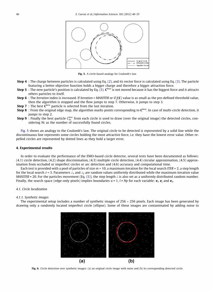
Fig. 5. A circle-based analogy for Coulomb’s law.

46 E. Cuevas et al. / Information Sciences 182 (2012) 40–55

Step 4 : The charge between particles is calculated using Eq. (2), and its vector force is calculated using Eq. (3). The particlefeaturing a better objective function holds a bigger charge and therefore a bigger attraction force.

Step 5 : The new particle’s position is calculated by Eq. (5). Cbest is not moved because it has the biggest force and it attractsothers particles to itself.

Step 6 : The Iteration index is increased. If Iteration = MAXITER or if J(C) value is as small as the pre-defined threshold value,then the algorithm is stopped and the flow jumps to step 7. Otherwise, it jumps to step 3.

Step 7 : The best Cbest particle is selected from the last iteration.Step 8 : From the original edge map, the algorithm marks points corresponding to Cbest. In case of multi-circle detection, it

jumps to step 2.Step 9 : Finally the best particle Cbest

Nc from each circle is used to draw (over the original image) the detected circles, con-sidering Nc as the number of successfully found circles.

Fig. 5 shows an analogy to the Coulomb’s law. The original circle to be detected is represented by a solid line while thediscontinuous line represents some circles holding the most attractive force, i.e. they have the lowest error value. Other re-pelled circles are represented by dotted lines as they hold a larger error.

4. Experimental results

In order to evaluate the performance of the EMO-based circle detector, several tests have been documented as follows:(4.1) circle detection, (4.2) shape discrimination, (4.3) multiple circle detection, (4.4) circular approximation, (4.5) approx-imation from occluded or imperfect circles or arc detection and (4.6) accuracy and computational time.

Each test is provided with a pool of particles of size m = 10, a maximum iteration for the local search ITER = 2, a step lengthfor the local search d = 3. Parameters k1 and k2 are random values uniformly distributed while the maximum iteration valueMAXITER = 20. For the particles movement (Eq. (5)), the step length k is also set as a uniformly distributed random number.Finally, the search space (edge-only pixels) implies boundaries u = 1, l = Np for each variable: ei, ej and ek.

4.1. Circle localization

4.1.1. Synthetic imagesThe experimental setup includes a number of synthetic images of 256 � 256 pixels. Each image has been generated by

drawing only a randomly located imperfect circle (ellipse). Some of these images are contaminated by adding noise to

Fig. 6. Circle detection over synthetic images: (a) an original circle image with noise and (b) its corresponding detected circle.

Fig. 7. Circle detection applied to two natural images, (a) the detected circle is shown near the wheel’s ring and (b) the detected circle is shown close to theball’s periphery.

E. Cuevas et al. / Information Sciences 182 (2012) 40–55 47

increase complexity in the detection process. The parameters to be estimated are the centre of the circle position (x,y) and itsradius (r). The algorithm is set to 20 iterations for each test image. In all cases, the algorithm has been able to detect thecircle’s parameters despite noise presence. The detection is robust to translation and scale, keeping a reasonable low elapsedtime (typically under 1 ms). Fig. 6 shows the circle detection over two different synthetic images.

4.1.2. Real-life imagesIn this experiment we test the circle detection algorithm upon real-life images. Twenty-five images of 640 � 480 pixels

are used in the test. All images have been captured using an 8-bit color digital camera and each natural scene includes a cir-cle shape among other objects. All images are pre-processed using an edge detection algorithm before applying the EMO’scircle detector. Fig. 7 shows two cases from 25 tested images.

Real-life images rarely contain perfect circles. Therefore the detection algorithm approximates the circle that adapts bet-ter to the imperfect circle, i.e. the circle corresponding to the smallest error in the objective function J(C). All results havebeen statistically analyzed to ease comparison. The detection time for the image shown in Fig. 7(a) is 13.540807 s whileit is 27.020633 s for the image in Fig. 7(b). The detection algorithm has been executed over 20 times on the same image(Fig. 7(b)), yielding the same parameter set: x0 = 214, y0 = 322, and r = 948. The proposed EMO algorithm was able to con-verge to the minimum solution as is referred by the objective function J(C).

Fig. 8. Circle detection on synthetic images: illustrations (a) and (c) show the original images while (b) and (d) show their corresponding detected circles.

Fig. 9. Different shapes embedded into real-life images, (a) the test image, (b) the corresponding edge map, (c) the detected circle and (d) the detected circleoverlaid on the original image.

Fig. 10. Multiple circle detection on real images: pictures in (a) and (c) show edge images as they are obtained from applying Canny’s algorithm. Images (b)and (d) present original scenes with the overlaid of detected circles being quite evident.

48 E. Cuevas et al. / Information Sciences 182 (2012) 40–55

E. Cuevas et al. / Information Sciences 182 (2012) 40–55 49

4.2. Shape discrimination

In this section we focus on the ability for detecting circles despite the presence of any other shape on the image. Five syn-thetic images of 540 � 300 pixels are considered for this experiment. Noise has been added to all images and a maximum of20 iterations was used for the detection. Two examples of circle detection on synthetic images are shown by Fig. 8.

The same experiment was repeated for some real-life images (see Fig. 9) confirming that the circle detection is completelyfeasible on natural images despite other shapes being present on the scene.

4.3. Multiple circle detection

The presented approach was also capable of detecting several circles over real-life images. In the first experiment, a max-imum number for circular shapes to be detected had been set. The algorithm works on the original edge-only image until thefirst circle is detected. The first circle represents the circle with the minimum objective function value J(C). Such shape isthen masked (eliminated) and the EMO circle detector continues operating over the modified image. The procedure was re-peated until the maximum number of detected circular shapes was reached. As a final step, all detected circles were vali-dated by analyzing their circumference continuity as proposed in [4]. Such procedure becomes necessary in case morecircular shapes are required in the future.

Fig. 10(a) shows the edge image after applying the Canny’s operator and Fig. 10(b) presents the actual image includingseveral detected circles which have been overlaid for presentation. Fig. 10(c) and (d) shows similar cases.

EMO algorithm takes the optimized image from the previous step as input. It is important to consider that the new inputdoes not contain any complete circle, because any other has already been detected and masked at the previous step. There-fore, the algorithm focuses on detecting other potential circles until the maximum of 20 iterations is reached.

4.4. Circular approximation

Since circle detection has been approached as an optimization problem, it is possible to approximate a given shape as theconcatenation of a number of circles. By using the multiple-circle feature of the EMO algorithm presented in the previoussection, the EMO algorithm may continually find circular shapes that may be gathered to resemble a non-circular shapeaccording to the values from the objective function J(C).

Fig. 11. Circular approximation: (a) the original image, (b) its circular approximation considering 3 circles, (c) another testing image, and (d) its circularapproximation considering 4 circles.

Fig. 12. Approximation of circles from occluded shapes, imperfect circles and arc detection: (a) the original image with 2 arcs, (b) the circle approximationfor the first image, (c) occluded natural image of the moon and (d) circle approximation for the moon example.

50 E. Cuevas et al. / Information Sciences 182 (2012) 40–55

Fig. 11 shows some examples of circular approximation. Fig. 11(a) presents a circular-like shape which may host a circularsuperposition. In that case, Fig. 11(b) features the approximation with 3 circles after applying the EMO multi-circle detector.Fig. 11(c) presents an ellipse that has been approximated by the concatenation of four circles as shown by Fig. 11(d).

4.5. Circle localization from occluded or imperfect circles and arc detection

Circle detection may also be useful to approximate circular shapes from arc segments, occluded circular segments orimperfect circles, all representing common challenges for typical computer vision problems. Again, EMO algorithm was ableto find the circle shape that approaches an arc segment according to the values in the objective function J(C). Fig. 12 showssome examples of such functionality.

4.6. Accuracy and computational time

This section discusses the algorithm’s ability to find the best circle considering synthetic images under noise presence.The experiment gets ten contaminated images of 256 � 256 pixels which contain only one circle centre at x = 128,y = 128, with r = 64 pixels. Two kinds of noise distributions are considered: the Salt & Pepper and the Gaussian noise.

Table 1Data analysis for images containing added Salt & Pepper noise.

Image properties Results

Error sum (Es) Computational time (s)

Size Circle center Radius Salt & Pepper level Total Mean Standard deviation Mode Mean Standard deviation

256 � 256 (128,128) 64 0.01 0 0 0 0 12.5505 0.5426256 � 256 (128,128) 64 0.02 0 0 0 0 13.0491 0.7455256 � 256 (128,128) 64 0.03 0 0 0 0 13.3401 0.7365256 � 256 (128,128) 64 0.04 0 0 0 0 14.3228 0.655256 � 256 (128,128) 64 0.05 2 0.0571 0.2355 0 14.2141 0.7982256 � 256 (128,128) 64 0.06 0 0 0 0 14.8669 0.9604256 � 256 (128,128) 64 0.07 3 0.0857 0.5071 0 15.3725 0.5147256 � 256 (128,128) 64 0.08 7 0.2 0.6774 0 14.5373 0.5147256 � 256 (128,128) 64 0.09 6 0.1714 0.5137 0 14.5747 0.8907256 � 256 (128,128) 64 0.10 28 0.8 2.1666 0 14.7288 0.8116

Fig. 13. Test images with added Salt & Pepper noise: (a) image holding 0.01 of added noise, (b) image including 0.05 of added noise, (c) image containing 0.1of added noise, and (d), (e) and (f) show the final 25 detected circles for each test image.

Table 2Data analysis following the Gaussian noise application.

Image properties Results

Error sum (Es) Computational time (s)

Gaussian noise

Size Circle center Radius Mean Standard deviation Total Mean Standard deviation Mode Mean Standard deviation

256 � 256 (128,128) 64 0 0.01 0 0 0 0 11.7008 0.6566256 � 256 (128,128) 64 0 0.02 0 0 0 0 12.8182 0.9257256 � 256 (128,128) 64 0 0.03 0 0 0 0 13.8073 0.6438256 � 256 (128,128) 64 0 0.04 6 0.1714 0.5681 0 13.7866 0.8309256 � 256 (128,128) 64 0 0.05 10 0.2857 0.825 0 14.0476 1.4691256 � 256 (128,128) 64 0 0.06 26 0.7429 0.95 0 14.0622 0.5463256 � 256 (128,128) 64 0 0.07 32 0.9143 1.961 0 14.6079 0.4346256 � 256 (128,128) 64 0 0.08 158 4.5143 11.688 0 14.1732 0.8198256 � 256 (128,128) 64 0 0.09 106 3.0286 6.5462 0 13.9074 0.8165256 � 256 (128,128) 64 0 0.1 175 5 8.7447 0 15.1276 0.8606

E. Cuevas et al. / Information Sciences 182 (2012) 40–55 51

EMO algorithm iterates 35 times per image and the particle showing the best fitness value is regarded as the best circlematching to the actual one in the image. The process was repeated over 25 times per image to test consistency. The accuracyevaluation was achieved by the Error sum (Es) which measures the difference between the ground truth circle (actual circle)and the detected one. The error sum is defined as follows:

Es ¼ jxd � xtruej þ jyd � xtruej þ jrd � rtruej; ð13Þ

where xtrue, ytrue, rtrue are the coordinates of the centre and the radius value of the ground truth circle in the image. Moreoverxd, yd, rd correspond to the values of centre and radius respectively after being detected by the method.

Fig. 14. Test images contaminated with Gaussian noise: (a) image holding 0.01 added noise, (b) image including 0.05 added noise, (c) image containing 0.1added noise while images, (d), (e) and (f) are showing the final 25 detected circles as overlaid for each test image.

Table 3Experimental results after applying the EMO circle detector to real-life images.

Image properties Results

Matching error (%) Computational time (s)

Image name Size Total Mean Standard deviation Mode Mean Standard deviation

Cue ball 430 � 473 28.1865 0.805 0.0061 0.8035 26.6641 1.4018Street lamp 474 � 442 19.0638 0.545 0.0408 0.5326 23.4763 1.7857Wheel 640 � 480 22.265 0.636 0.0062 0.6336 31.356 1.4351

52 E. Cuevas et al. / Information Sciences 182 (2012) 40–55

The first experiment considers contaminated images doped with Salt & Pepper noise. The EMO parameters are: maximumiterations MAXITER = 35; for the local search, d = 4 and ITER = 4. The added noise is produced by MatLab�, considering noiselevels between 1% and 10%. The resulting values for Es and the computing elapsed time are reported in Table 1. Fig. 13 showsthree different images as examples, including 25 detected circles that are overlaid on each original image. It is evident fromFig. 13 that a higher added noise yields a higher dispersion on the detected shapes.

The second experiment explores the algorithm’s application to images contaminated with Gaussian noise. By definition,Gaussian noise requires a threshold value to convert each value to binary pixels yielding an image exhibiting more noisethan the Salt & Pepper contamination. Addition of Gaussian noise falls between 1% and 10%. The resulting values for Esand the computing elapsed time are reported in Table 2. Fig. 14 shows three different images as examples, including theoverlay of the 25 detected circles. Again, it is evident that the dispersion on the detected circles increases proportionallyto the added noise.

A similar test has been applied to different real images. It is important to mention that the Error sum (Es) is not used be-cause the coordinates for the centre and the radio for each circle are unknown. Table 3 shows the results after applying theEMO circle detector considering the algorithm for natural image presented in Fig. 15. The final 25 detected circles are over-laid over the original images.

Fig. 15. Real-life images used in the experiments, (a) cue ball, (b) wheel, (c) street ball, including the overlaid detected circles.

E. Cuevas et al. / Information Sciences 182 (2012) 40–55 53

5. Conclusions

This paper has presented an algorithm for the automatic detection of circular shapes among cluttered and noisy imageswith no consideration of the conventional Hough transform principles. The work describes a circle detection method whichis based on a nature-inspired technique known as the Electro-magnetism Optimization (EMO). It is a heuristic method forsolving complex optimization problems inspired by electro-magnetism principles. To the best of our knowledge, EMO algo-rithm has not yet been applied to any image processing task up to date. The algorithm uses the encoding of three non-col-linear edge points as candidate circles (x,y,r) in the edge-only image of the scene. An objective function evaluates if suchcandidate circles (charged particles) are actually present. Guided by the values of this objective function, the set of encodedcandidate circles are evolved using the EMO algorithm so that they can fit into the actual circles on the edge-only map of theimage. From our results, the EMO approach has been capable of effectively detecting circular shapes embedded into compleximages with little visual distortion despite the presence of noisy background pixels and still shows good accuracy andconsistency.

An important feature is to consider the circle detection problem as an optimization approach. Such a view enables theEMO algorithm to find circle parameters according to J(C) instead of voting all possible chances for occluded or imperfectcircles as other methods do.

Although Hough transform methods for circle detection also uses three edge points to cast one vote for the potential cir-cular shape in the parameter space, they would require huge amounts of memory and longer computational times to obtaina sub-pixel resolution. In the HT-based methods, the parameter space is quantized and the exact parameters for a valid circleare often not equal to the quantized values. This fact evidently yields a non-exact determination for a circle actually presentin the image. However, the proposed EMO method does not employ the quantization of the parameter space. In our ap-proach, the detected circles are directly obtained from Eqs. (6)–(9) effectively detecting the circle with sub-pixel accuracy.

Although the results offer evidence to demonstrate that the EMO method can yield good results on complicated and noisyimages, the aim of our paper is not to devise a circle-detection algorithm that could beat all currently available circle detec-tors, but to show that electro-magnetism systems can be effectively considered as an attractive alternative for detecting cir-cular shapes.

Acknowledgments

Humberto Sossa would like to thank SIP-IPN under Grant No. 20100468 for its economical support. The authors thank theEuropean Union, the European Commission and CONACYT for the support. This paper has been prepared by an economicalsupport of the European Commission under grant FONCICYT 93829. The content of this paper is an exclusive responsibility ofthe UDEG and the CIC-IPN and it cannot be considered a reflection of the European Union position. The proposed algorithm ispart of the vision system used by a biped robot supported under the grant CONACYT CB 82877.

54 E. Cuevas et al. / Information Sciences 182 (2012) 40–55

References

[1] F.A. Andalóa, P.A.V. Miranda, R.S. Torres, A.X. Falcão, Shape feature extraction and description based on tensor scale, Pattern Recognition 43 (2010) 26–36.

[2] N. Andrei, Acceleration of conjugate gradient algorithms for unconstrained optimization, Applied Mathematics and Computation 213 (2009) 361–369.[3] T.J. Atherton, D.J. Kerbyson, Using phase to represent radius in the coherent circle Hough transform, in: Proceedings of the IEEE Colloquium on the

Hough Transform, IEEE, London, 1993.[4] V. Ayala-Ramirez, C.H. Garcia-Capulin, A. Perez-Garcia, R.E. Sanchez-Yanez, Circle detection on images using genetic algorithms, Pattern Recognition

Letters 27 (2006) 652–657.[5] X. Baia, X. Yangb, L. Jan-Latecki, Detection and recognition of contour parts based on shape similarity, Pattern Recognition 41 (2008) 2189–2199.[6] J. Becker, S. Grousson, D. Coltuc, From Hough transforms to integral transforms, in: Proceedings of the International Geoscience and Remote Sensing

Symposium, IGARSS-02, 2002, pp. 1444–1446.[7] C. Blum, Ant colony optimization: introduction and recent trends, Physics of Life Reviews 2 (2005) 353–373.[8] G. Bongiovanni, P. Crescenzi, Parallel simulated annealing for shape detection, Computer Vision and Image Understanding 61 (1995) 60–69.[9] J.E. Bresenham, A linear algorithm for incremental digital display of circular arcs, Communications of the ACM 20 (1977) 100–106.

[10] U.K. Chak, Genetic and evolutionary computing, Information Sciences 178 (2008) 4419–4420.[11] W. Dua, B. Li, Multi-strategy ensemble particle swarm optimization for dynamic optimization, Information Sciences 178 (2008) 3096–3109.[12] M. Fischer, R. Bolles, Random sample consensus: a paradigm to model fitting with applications to image analysis and automated cartography, CACM 24

(1981) 381–395.[13] M. Graña, Evolutionary algorithms, Information Sciences 133 (2001) 101–102.[14] T. Gruber, Collective knowledge systems: where the social web meets the semantic web. Web semantics: science, Services and Agents on the World

Wide Web 6 (2008) 4–13.[15] J.H. Han, L.T. Koczy, T. Poston, Fuzzy Hough transform. In: Proceedings of the 2nd International Conference on Fuzzy Systems, 1993, pp. 803–808.[16] M. Hongwei, Handbook of Research on Artificial Immune Systems and Natural Computing: Applying Complex Adaptive Technologies, IGI Global, 2009.[17] B. _Ilker, S. Birbil, F. Shu-Cherng, An electromagnetism-like mechanism for global optimization, Journal of Global Optimization 25 (2003) 263–282.[18] B. _Ilker, S. Birbil, F. Shu-Cherng, R.L. Sheu, On the convergence of a population-based global optimization algorithm, Journal of Global Optimization 30

(2004) 301–318.[19] J. Jhen-Yan, L. Kun-Chou, Array pattern optimization using electromagnetism-like algorithm, AEU – International Journal of Electronics and

Communications 63 (2009) 491–496.[20] D. Karaboga, B. Akay, A comparative study of artificial bee colony algorithm, Applied Mathematics and Computation 214 (2009) 108–132.[21] C.H. Lee, F.K. Chang, Fractional-order PID controller optimization via improved electromagnetism-like algorithm, Expert Systems with Applications 37

(2010) 8871–8878.[22] Y.H. Lina, C.H. Chen, Template matching using the parametric template vector with translation, rotation and scale invariance, Pattern Recognition 41

(2008) 2413–2421.[23] J. Liu, K. Tsui, Toward nature-inspired computing, Communications of the ACM 49 (2006) 59–64.[24] V. Loia, Soft computing meets agents, Information Sciences 176 (2006) 1101–1102.[25] E. Lutton, P. Martinez, A genetic algorithm for the detection 2-D geometric primitives on images, in: Proceedings of the 12th International Conference

on Pattern Recognition, 1994, pp. 526–528.[26] P. Lévy, From social computing to reflexive collective intelligence: the IEML research program, Information Sciences 180 (2010) 71–94.[27] J.A. Martın, M. Santos, J. de Lope, Orthogonal variant moments features in image analysis, Information Sciences 180 (2010) 846–860.[28] A. Moliton, Basic Electromagnetism and Materials, Springer-Verlag, 2007.[29] H. Muammar, M. Nixon, Approaches to extending the Hough transform, in: Proceedings of the International Conference on Acoustics, Speech and

Signal Processing ICASSP-89, 1989, pp. 1556–1559.[30] Z. Naji-Azimi, P. Toth, L. Galli, An electromagnetism metaheuristic for the unicost set covering problem, European Journal of Operational Research 205

(2010) 290–300.[31] B. Naderi, R. Tavakkoli-Moghaddam, M. Khalili, Electromagnetism-like mechanism and simulated annealing algorithms for flowshop scheduling

problems minimizing the total weighted tardiness and makespan, Knowledge-Based Systems 23 (2010) 77–85.[32] H. Qia, K. Lia, Y. Shena, W. Qu, An effective solution for trademark image retrieval by combining shape description and feature matching, Pattern

Recognition 43 (2010) 2017–2027.[33] A. Rocha, E. Fernandes, Hybridizing the electromagnetism-like algorithm with descent search for solving engineering design problems, International

Journal of Computer Mathematics 86 (2009) 1932–1946.[34] A. Rocha, E. Fernandes, Modified movement force vector in an electromagnetism-like mechanism for global optimization, Optimization Methods &

Software 24 (2009) 253–270.[35] P.L. Rosin, Further five point fit ellipse fitting, in: Proceedings of the 8th British Machine Vision Conference, Cochester, UK, 1997, pp. 290–299.[36] P.L. Rosin, H.O. Nyongesa, Combining evolutionary, connectionist, and fuzzy classification algorithms for shape analysis, in: S. Cagnoni et al. (Eds.),

Proceedings of the EvoIASP, Real-World Applications of Evolutionary Computing, 2000, pp. 87–96.[37] G. Roth, M.D. Levine, Geometric primitive extraction using a genetic algorithm, IEEE Transactions on Pattern Analysis and Machine Intelligence 16

(1994) 901–905.[38] K. Schindlera, D. Suterb, Object detection by global contour shape, Pattern Recognition 41 (2008) 3736–3748.[39] M.C. Schut, On model design for simulation of collective intelligence, Information Sciences 180 (2010) 132–155.[40] D. Shaked, O. Yaron, N. Kiryati, Deriving stopping rules for the probabilistic Hough transform by sequential analysis, Computer Vision Image

Understanding 63 (1996) 512–526.[41] D. Teodorovic, Swarm intelligence systems for transportation engineering: principles and applications, Transportation Research Part C: Emerging

Technologies 16 (2008) 651–667.[42] J. Tiana, W. Yub, L. Ma, AntShrink: ant colony optimization for image shrinkage, Pattern Recognition Letters 31 (2010) 1751–1758.[43] C.S. Tsou, C.H. Kao, Multi-objective inventory control using electromagnetism-like metaheuristic, International Journal of Production Research 46

(2008) 3859–3874.[44] J.R. Van-Aken, An efficient ellipse drawing algorithm, CG& A 4 (1984) 24–35.[45] P. Wu, Y. Wen-Hung, W. Nai-Chieh, An electromagnetism algorithm of neural network analysis an application to textile retail operation, Journal of the

Chinese Institute of Industrial Engineers 21 (2004) 59–67.[46] L. Xu, E. Oja, P. Kultanen, A new curve detection method: randomized Hough transform (RHT), Pattern Recognition Letters 11 (1990) 331–338.[47] J. Yao, N. Kharma, P. Grogono, Fast robust GA-based ellipse detection, in: Proceedigns of the 17th International Conference on Pattern Recognition

ICPR-04, Cambridge, UK, 2004, pp. 859–862.[48] H. Yin, W. Huang, Adaptive nonlinear manifolds and their applications to pattern recognition, Information Sciences 180 (2010) 2649–2662.[49] C. Ying-ping, J. Pei, Analysis of particle interaction in particle swarm optimization, Theoretical Computer Science 411 (2010) 2101–2115.[50] H. Yuen, J. Princen, J. Illingworth, J. Kittler, Comparative study of Hough transform methods for circle finding, Image and Vision Computing 8 (1990)

71–77.[51] S. Yuen, C. Ma, Genetic algorithm with competitive image labelling and least square, Pattern Recognition 33 (2000) 1949–1966.

E. Cuevas et al. / Information Sciences 182 (2012) 40–55 55

[52] A. Yurtkuran, E. Emel, A new Hybrid electromagnetism-like algorithm for capacitated vehicle routing problems, Expert Systems with Applications 37(2010) 3427–3433.

[53] Q. Zhang, M. Mahfouf, A nature-inspired multi-objective optimization strategy based on a new reduced space search ing algorithm for the design ofalloy steels, Engineering Applications of Artificial Intelligence (2010), doi:10.1016/j.engappai.2010.01.017.

[54] X. Zhang, P.L. Rosin, Superellipse fitting to partial data, Pattern Recognition 36 (2003) 743–752.