Lit

FPFACE.

The following thesis, submitted to the University of Tasmania

for the degree of Doctor of Science, consists of two main sections,

complete details of which may be found on lat. (ii)-(v). The parts

marked Eli -(0 represent published papers, whilst f3 -W have

been submitted for publication to the Acta Mathematica and the

Annals of Mathematics respectively. The rest consists of a number

of hitherto unpublished papers.

The work was carried out indeendently by the candidate, and

the various ideas underlying the construction of the algebraic

optics here presented, as well as the methods of dealing with

invariant action principles are due to him. Further details may

bB found on pa. 3, 34=9 i49 ., etc.

Of two papers photostatic copies of proofs are given, as

reprints have not yet been received. In accordance with the rules

governing the degree, two papers on the Axiomatic Treatment of

the Second Law of Thermodynamics, (due to appear in the American

Journal of Physics in December 1948), have also been included.

September, 1948.

rote: Throughout this thesis, underlined symbols are to be

read as follows:

Red Clarendon type,

Green German (Gothic)type,

Black Italics.

SECTION A : OPTICS.

ALVBRAIC METHODS FOR THE lET'BRMINATION OF TH -fl GEOMWRICAL HIGH4R ORDJ-IIR ABDRRATIONS OF OPTICAL SYSTEi;iS.

page I. Tangential Aberrations of a System of Coaxial Spher-

ical Refracting Surfaces. [11

t. Abstract.- Index of Symbols. 1 2. Introduction. . 3

3. Definition of the aberrations, 4 4. Associated rays. • 5

5. Principles of the present method. 7 6. g-Polynomials. 9

7. Expansion of ili. to a. Expansion of i.e. tt 2. Change of position of object or of focal plane. 13

10. The diaphragm. 14

11. v', and spherical aberration. 15 12. Distortion. 16

13. Coma and curvature of field. 17

144 Principles of an alternative method. 18 15. Example of computations.(2 tables and to diagrams). 19 16. Conclusion. , 31

II. Aberrations of systems of coaxial spherical refracting surfaces. Abstract 32

Part I. Theory in General. 34

1. General introduction. 34 2. Notation. 37

3. Definition of the aberration of a ray. Order. uasi-Invariants-

4. Quasi-linear variAbles. Canonical coordinates. 46 8. Iteration. 52 6. The diaphragm. 56 7. Shift of image plane. 59 8. Shift of diaphragm. 60 O. Change in position of object. 63 to. Reversed optical systems. 65 11. Addition of optical systems. 66 12. General linear coordinates. 69 13. On the classification of aberrations. 74

39

Uty)

Part II. Algebraic Developmeitts. ddentities. 14. Plane of incidence. Invariance of K. 16. Expression for 4, Ad* -. 16. Standard form of primary aberrations. 17. Identities.

page 78

78

8

8±

83

Part III. Explicit Series Expansions. Sample Computations. 95

Is. On alternative methods of calculation. 95

19. First method in general. Canonical coordinates. 96.

20. First method ctd. Lower orders in canonicalcoardinatEn. 99

. 21. Iteration in explicit form. 105

22. Jacoby polynomials. 107

23. First method. Lower orders in semi-canonical variables. 109

24e Second method. All orders. 111 -

25. Sample computation. (2 tables, 8 diagrams) 112

26. Application of identities. (Checks). (1 table). 131

27. Conclusion. List of symbols. References. 124

III. Algebraic Theory of the Primary Aberrations of the Symmetrical Optical System. bo 142

IV. Aberrations of the General Symmetrical Optical System. Abstract. 148 l e Introduction. 149 2. Specification of surfaces. 151 3. Refraction at a surface. 153. 4. Expression for 4. 126. 5. Determination of a, , 156 6. Expansions in terms of %, and of g 1 1,4 . 157 7. Solution of the equation for S. 168 6. Introduction of the Y i . 160

9. Final expressions for 44.. 161

lo. Special surfaces. 162 ii. On the design of systems with aspherical surfaces. 165 12. Example of the application of the method.(1 table). 169 13. Comparison of results with trigonometrical traces.(7n124172 1.4. Conclusion. Table of symbols. References. 166.

V. Supplementary results concerning the aberrations of the general SyMmetrical Optical System. - (Abstract:) 190

part I. On the Computation of Tertiary and Higher Order Abeiu,ations. 191

1. Introduction. 191 2. Fundamental Sets of terms. 192 3. Solution of the equation for Se 193 4. Exgession for Ail. 194 5. Sn$YroOnyTn y. for n = 1,20. 195

page 6. On the computation of tan, (n=1,2,6). 196 7. Spherical surfaces. &98

6. Tertiary increments in explicit form. 199 9. Conclusion. 20?

Part II. The Geometrical Aberrations of Optical Systems with Continuously Varying Refractive Index.

to. Introduction. tt. The 'continuous' symmetrical optical system. 12. On the associated linear equation. p. and a solutions. 13. On the solution curves of the linear equation. 14. Introduction of Mx). 16. Aberrations in general. 16. Primary aberrations. 17. Aberrations of higher order. Iteration. 18. Secondary aberrations. 19. On the limiting case of a k-surf ace system, as k-+0,0. 20. Conclusion. List of symbols.

Part III. On the Sine Relation

21. The case of systems of coaxial refracting surfaces of revolution.

22. Generalisation of K. 23. The sine relatio4 in the general case.

SECTION B : ACTION INTEGRALS - RELATIVITY.

ON TENSORS ARISING FROM COORDINATE-INVARIANT AND GAUGE- INVARIANT ACTION INTEGRALS.

VI. On Eddington's Higher Order Equations of the Gravitational Field. L4

VII. The Hamiltonian Derivatives of a Class of Fundamental Invariants. W

VIII. A Special Class of Solutions of the Equations of the Gravitational Field Arising from Certain Gauge-invariant Action Principles. Ekj

209

211

213

214

216

217

217

220

221

222

233

230

230

231

233

236

242

252

contd.

60

page

IX. Uber die Variationsableitung von Fundamentalinvarian-ten beliebig hoher Ordnung. DI 255

X. On the Hamiltonian Derivatives Arising from a Class of Gauge-Invariant Action Principles in a W. [73 267

XI. An Identity between the Hamiltonian Derivatives of Certain Fundamental Invariants in a W4. [s] 28 4

XII. On a Set of Conform-invariant Equations of the Gravitational Field. 288

pEcTiox C : Two Papers concerned with the Axiomatlg. Treatment of Itlf_gecond Law Q

XIII. On the Principle of Caratheodory. (9] 295

XIV. On the Theorem of Caratheodory. (Ao3 304.

This article has been removed for copyright or proprietary

reasons.

It has been published as: Buchdahl, H. A., 1946. The algebraic analysis of the higher-order aberrations of optical systems : tangential aberrations of a system of coaxial spherical refracting surfaces, Proceedings of the Physical Society, 58(5), 545-575

THE ALGEBRAIC THEORY AND CALCULATION OF THE GEOMETRICAL

HIGHER ORDER ABERRATIONS OF OPTICAL SYSTEMS.

I: Aberrations of systems of coaxial spherical refractinA surfaces.

by H. A. Buchdahl.

Dept. of Physics, University of Tasmania.

Abstract: Defining the aberration. of a ray in terms of the components

of the displacement of its point of intersection with a chosen

plane of reference from an ideal image point in the same plane,

a theory of higher order aberrations is developed by means of

elementary algebraic methods. The treatment rests in principle

upon the study of the departure from exact linearity of the

relations connecting the variables specifying the ray at the

different surfaces of an optical system. This leads in practice

to the possibility of computing the exact aberration coefficients

to any order desired without the neeessity of any trigonometrical

tracing. Unrestricted changes in the position of object, diaphragm

or plane of reference are easily dealt with in practice, the

aberration coefficients being pure constants of the system.

A number of special problems are briefly considered, such as the

addition of different optical systems, and the aberrations of

reversed systems.

As a practical example the computations necessary for the

determination of the complete exact primary and secondary '

-2-

aberrations, and of the tertiary spherical aberration are

given in detail for the case of a Cooke Triplet illustrating

the relatively small amount of labour involved. A number

of diagrams illustrate the good agreement between the

aberrations predicted by the present method and those obtained

by means of strict trigonometrical tracing.

PART I. THEORY IN GENERAL.

f 1. General Introduction.

(a)

In the present paper, which is a continuation of the author's

previous work (Buchdahl, 1946), a general algebraic theory of

the monochromatic aberrations of systems of coaxial spherical

refracting surfaces will be developed. The previous restriction

to tangential rays is now removed, all rays capable of passing

through the system being allowed. Since a ray is now specified

by four co-ordinates instead of only two the theory may be

expected to be somewhat more complex. Accordingly certain

changes have been made in the method and notation used previously

for the sake of simplicity of development as well as of uniformity

of notatioh. In particular, considerable use has been made of

an extension of the method outlined in (14 of the paper referred

to above. This leads in practice to the possibility of

computing the exact aberration coefficients, suitably defined,

by means of an iterative method to any order desired. The

calculation of the fu3L quaternary or higher aberrations will

usually be too lengthy to be worthwhile. The computing scheme

gives the individual contributions of the different surfaces,

and may be arranged so as to allow of a simple but complete

investigation of unrestricted changes in the positions of

object, diaphragm and plane of reference. It may be remarked

that Berzberger states (Herzberger, 1931 (b)) that equations

for the dependence of aberrations on object position are given

by him for the first time (loc. cit. 11,. 115); but he confines

-4 -

htnself entirely to a theoretical discussion of the primary

terms. It should be stressed that aberrations of order higher that

the first depend somewhat on the co-ordinates used unless those of

lower order vanish identically: the differences between the

results obtained with different co-ordinates are implicitly

compensated by the appropriate remainder terms.

(b )

In principle the simplicity of the method appears to arise mainly

from three factors: first, the use of quasi-invariants,

expressions which reduce to optical invariants in the paraxial

limit (3). These automatically render the derivation of explicit

summation theorems unnecessary. Secondly, the choice of special

systems of co-ordinates, below called canonical, which consist of

two particular pairs of so-called linear co-ordinates (4).

Thirdly, the construction of expressions which closely resemble the

linear relations of paraxial theory and which clearly indicate the

departures from linearity; and it is these which make iteration

possible (4g4b. and 5).

When canonical co-ordinates are used the aberration coefficients

are pure constants of the system, in the sense that they do not

invblve the positions of the object, diaphragm or plane of reference.

However, if desired, general linear co-ordinates may be used (§l2.),

such as pairs of co-ordinates in object and image space, etc.

Special attention is paid below to co-ordinates closely resembling

canonical co-ordinates (4c.), the use of which makes it possible

directly to employ pairs of direction cosines in the object space

and image space respectively in order to specify the ray. This

may be of same importance in any problems involving

-5-

the use of the angle eikonal. When the system is telescopic

this particular set of co-ordinates is forbidden. But we may

be certain that canonical co-ordinates are always allowed.

(0)

It may be remarked that the length of a synthetic algebraic

theory as compared with a development along the lines of

Hamilton's analytic method (1.E. Steward, 1928 (a)) is somewhat

deceptive. This is mainly due to the feet that the aims of

these rival theories do not coincide. No doubt Hamilton's

method is best suited to the most general abstract development

of geometrical optics. In the present paper, however, an

attempt has been made to find the best compromise between

brevity and elegance on the one hand and practical usefulness

on the other: in particular as regards the actual calculation

of the aberrations of higher order in the presence of those of

lower order; whilst same writers on the subject seam to pay

little attention to this problem (1.1. Herzberger, 1931 (a)).

Our use of co-ordinates lying entirely in the object space

contributes greatly to the ease with which practical problems

may be handled (E. Herzberger, 1931 (c)); and no constants are

introduced which cannot be straightforwardly determined in

practice by the methods described below. Restriction to primary

aberrations allows certain modifications to be made which render

the method of quasi-invariants very valuable from a didactic point

of view. In particular, the usual expressions for the Seidel

aberrations (16) may be derived in a manner probably more suitable

for undergraduate teaching than the usual developments (s.,g,.

Whittaker, 1915(a), or Conradv, 19291a))

(a)

-6-

It will be noticed that virtually all the lengthy and

cumbrous parts of the theory arise in the attempt to make

the necessary calculations sufficiently brief to be useful

in practice. The simplicity of the equations(20.41) and

(20.42) in conjunction with (21.2) for instance shows that

the somewhat laborious developments in Part III are amply

justified.

§ 2. Notation.

For convenient reference a table containing most of the

symbols employed in the text is given at the end of this

paper in §27.

The quantities Li( Fr- Lad, H0a - HBO, Cy , Up U t I f U0 ,

0, N, r, dt are essentially the same as those used by Conrady

(Conradv, 1929 (b)); although these are not used finally

they are employed at first in order to make the transition

to canonical variables more transparent to the practical

worker. The equations determining the passage of a skew

ray through a surface are

tan Uc = L-r (2.1)

tan 0 _ tan Uz . (2.2) sin(Uy-X0 )

sin Uz sin U = (2.3) sin 0

sin I = H sin u (L-Osin U (2.4)

r sin Uz r cos Uz

-7-

.64N sin I) = 0

A(' + U) =

together with the equations (2.1) - (2.4), with H, L, Up

Up 1 replaced by the corresponding dashed symbols. The

transfer equations are .

(U )1 Y

. = (U'). Y J 4

(2.5)

(2.6)

(2. 71)

(Uz )iii. = (U;)j (2.72)

E1j+

1 = H! (2.73) J

Liji.1

= L' - d (2.74) i •

Notice that we have taken H to be positive when it lies

below the a - axis, the co-ordinate system being left-handed,

nix, yA

A s x The axis lies in the direction of the axis of symmetry of

the system. & coincides with the pole of the refracting

surface in question, them, y. plane coinciding with the

tangential plane.

As regards the notation employed it may be remarked that the

number of symbols used has been reduced to a minimum by the

frequent and, above all, systematic use of affixes. Even so,

duplication of certainn symbols was unavoidable in some cases.

But it is hoped that this will not lead to confusion.

(b)

The numbered equations in-the author's previous paper

(Buchdahl, 1946) will be distinguished by the letter T;

thus (T 5.8). A homogeneous polynomial of degreq 2n+1

in a set of linear variables (w.§4) will be said to be of

the a th order. The phrase "correct to the n th order" as applied to any expression, means that it holds when terms

of order exceeding n are neglected. By analogy with usual

mathematical notation the symbol 0(n) is used to represent

a term or terms the degreit of which is not less than n.

§3. Definition of the Aberrations of a Rev. Order. Quasi-Invariants.

(a)

Let us take all paraxial rays always to lie in the tangential

plane. Given two arbitrary paraxial rays (y1 , ul ) and ol)

the expression

= N( t - Z)uu (3.1)

is an optical invariant according to (T 4.6). That is, for all

and = X / j+1

so that has the same value everywhere in the optical systen.

Let 0 be an object point lying in the tangential plane,

whilst the "axial point of the object 0 0" is the perpendicular

projection of 0 on to the principal axis. Then the position

of 0 may be specified by the position la of 00 with respect

-9-

to the first surface and by the distance 0 00 =h1. Moreover

it is convsnient to distinguish quantities referring to an

"axial ray" (a ray through 00) by the additional subscript o.

If the two rays in (3.1) be taken to be respectively an

axial ray and a ray through the object point, then

Xi = - /duo uj = hi uo

(3.31)

is an optical invariant (Lagrange, or Smith-Helmholtz invariant).

If the suffix k refers to the last surface throughout, the

paraxial magnification of the system ml (=I/a) is defined as

hitc Niuci M I = = by (3.31)

h i Niu0k 1

1.1 7' p say.

(3.32)

( 3.21 )

Since the right-hand side of (3.32) depends only upon G ol

it follows that all rays through 0 on emerging from the system

pass through a certain point 0', usually referred to as the

ideal blame point, the position of which is defined by t

and hk '• The plane perpendicular to the principal axis which

passes through the image point 00 ' conjugate to 00 is the

paraxial or ideal image Planeu and 0' is situated in the latter.

Since kt is proportional to ILI a linear object lying in the

abject plane will have a perfect image lying in the ideal image

plane.

-10-

(b) Considering now actual rays passing through the system

these will not in general intersect the ideal image plane

in the point 0'. Let the ray intersect the 1th "object

plane" in the point given by the rectangular co-ordinates

Hyj, Hzj . If the ray passed through the systan according

to the laws of paraxial imagery the co-ordinates of this

point would be byj , hmj . Then the components of the aberration

of the ray before the jth surface are

8 yj

= ELYJ

- Ii Y3

= H -h zj zj zj

(3.4)

Since the optical eystan is symmetrical we may without loss of

generality take the object point to lie in the tangential plane.

In that case hij = 0 1 and h4li will be written hi. The sign

convention for Hy , and Hz is the same as that which applies

to H. (v.42a).

In order to avoid unnecessary duplication of many equations

we shell make use of the convention that a symbol in Clarendon

type shall represent the two corresponding quantities referring

to the i and z axes; thus §j stands for both eyj and

e Also the general suffix J. 'ill be omitted whenever ze

confusion is not likely to arise thereby. Eq. (3.4) then reads

simply

= H - h (3.41)

Corresponding to the quantity A in (3.31) we may write down

the two expressions

A = Nuo H (3.5)

Then = ANuo H = A N u0c (3.51)

since A N h = 0 (3.511)

Between the two "components" of AN u c e there exists the

remarkable identity

uc ey see U cotan 06Nu0 ez (3.6)

This may be proved as follows: frcm elementary considerations

we have

= (to - L) tan Uy H

Hz = ( 0- L) tan Uz see Uy (3.61)

Hence

6Nu0 ey - sec Uc cotan 06Nit0ez

=411,u0 {H+ (to - L) [tan Uy - tan Uz sec Uy sec U0 cotan 01.1

=ANu0{H+ (t o - L)[tan Uy - sin(Uy-Udsec Uy sec U0]), by (2.2)

=4Nu0 l(L r)tan Uc (t - L)ten Uc I by (2.4)

=,tan. Uc 6 co 0 9 by (T 1.6),

Q.E.D .

c_r•-

-12-

(c) Now since = 1,2, ... ,k-i) (3.7)

we can write at once

= A + tiA.• -k -t -J

= A + k ' I say -1 -

which shows how is made up of the contributions LA i of

the individual surfaces. In order to fix our ideas we must at

this stage agree on some definite method of specifying a particular

ray. Accordingly at any surface let Y, Z be the co-ordinates

of the point of intersection of the ray with the tangent plane

to the pole of that surface; also let (1, -0, -Y) be the

direction cosines of the ray, so that

sin U cos Uz

/ (3.8)

sin Us

Then we may specify the ray by the four co-ordinates Y1 , ZI ,

Vit W 1 where 1

V =Pia

=

...

may now be looked upon as a definite function of those four

co-ordinates. To obtain this function in a closed form is out

of the question in all but the simplest cases. Accordingly let

(and so §I') be expanded in a Taylor series. In virtue

of the existence of an ideal image point the linear terms must

a cos U cos Uz

where = y 2+ Z2

= YV +ZW

C = y 2 + w 2 1.

-13-

be absent in this expansion. And since the system is symmetrical,

AA. must transform in the ssane way as / with respect to a

rotation of the system. It follows that at any surface A A

will be of the form

= lE+ + 61171 -I. eXIC BY-1

- 2-1 - 21 31 - 31 + + + S5 XiliC + 35 .111-K' + 86 Xi 2

-

•

16M2 7E, y7i (3.9)

and the • a, 1 9 are constants.

Clearly (3.9) consists of a series of homogeneous polynomials

of degree 3, 5, 7, •... Accordingly we shall call the poly-

nomial of degree 2n +1, (n = 1, 2, ...) the nth order

contribution (by. the j.th surface) to the aberration. The

aberration of order is then simply the sum of the contributions

divided by

/- 1 Thus if we write A. a„ vz,

Ai =a

and similarly for all other coefficients then

} (3.92)

= + • • • + + S:k .. (3.93)

-14-

It. mil be noticed that the nth order polynomial involves

(3.94) (n 4. 1) (n 4. 2)

coefficients (w.f17d).

(d) In the paraxial limit Ai reduces to an optical invariant.

In general we shall call any expression a quasi-invariant

if it reduces to an optical invariant in the paraxial limit.

And, as above, the change in a quasi-invariant in its passage

across a refracting surface is of degree 33 in the co-

ordinates.

(0)

It will be found convenient sometimes to write down all

terms of the expansion (3.9). If the coeffieients of the

terms of the nth order in pA j are g., g (-) . then we may

write

ea 4. Vv" y cv A A ; = zzz g y °"isvi.1 Tsr..1 )P.O

(3.10)

co Thus for example goo,i • • • g •s g ; •

Corresponding to (3.92) we have now

ho G • Pv4

G -

= gen) mi lAv3gt

— g fAvA 1 C47.1 • '

mtilst in the case of the dashed constants the summation is

again to be extended to a = instead of to (If

=0, the symbol i2 is to be interpreted am zero).

-15-

f4. Quasi-Linear Variables. Canonical Co-ordinates.

(a)

In order to be able to carry out the expansions of i 3.c.

by a process of iteration (ir. f 5) it is necessary first to

find explicit expressions for the departure from linearity

of certain relations which have exaqtiv linear equations as

their paraxial counterparts. Let us briefly consider the

Latter.

A paraxial ray :(y, has associated with it at any

surface the quantities .4e E0 10 etc. Any pair of

these may be used to specify the ray, provided they are

independent. Then we shall call those quantities linear

variables which are obtainable by a linear combination of

1.1 and 2 .2•1. Yj2 (19 rip iip p or au,, 4. Wit

(a, b = const); etc.

If therefore 4.i stands for any linear variable there

will be a relation of the form

PJ qiut

in which the al J .9 CIL are pure constants of the system. P qi

These are easily obtained in practice. It is only necessary

to trace two (paraxial) rays, the "2-ray" (1, 0), and

the "2-ray" (0, 1). Then the actual value of a, j in the former trace will be et • and the value of a. in the

latter will be ol q.1

(4.1)

-16-

4 ?

We have the identity

Ypj Yqjl

U U.pi

N

N.

which fhllows at once from (3.21) for the special case of the

rays (1, 0) and (0, 1). From (4.11) we find easily

(4.11)

Up uqj N 1 •= A =

i. • and rj u say. (4.12)

In place of yo ga.. in (4.1) any other two independent linear

variables might have been chosen, resulting in a different set

of paraxial coefficients. But these can always be expressed

in terms of the basic set above. (o also (12.2)).

Considering now non-paraxial rays, any variable which reduces

to a linear variable in the paraxial limit will be called ouasi-

linear, or sometimes simply Linear. If we choose four particular

quasi-linear variables associated with a ray then these may be

used to specify the latter; they are conveniently called the

co-ordinates of the ray. The four variables of §3.c,

Y 1 , Z 1 , V1 , Wit are a particularly convenient set of co-ordinates;

and we shall in future refer to them as canonical. (Linear

co-ordinates in general are considered in 112). By definition

we must have

Yqj + 2. (3)

upi Xi+ uqj Ii + o (3) (4.2)

-17-

We now require explicit expressions for the remainder terms,

which here appear merely as OW. Without these, any attempt

to calculate the higher order aberrations would be futile.

Replacing the axial ray in (3.71) by an arbitrary paraxial

ray

+ z An u • - v

where now Ay

•

Kit.4( t L)tan U 4- Id

AZ = NM. ( - Wtan. Uz sec U7

(4.21)

(4.211)

By definition Y = LV H = L tan U7 H

LW = L tan Ug sec Uy

so that (4.21) becomes

4.212)

N4(yJ - mij = -uY 1)+zA—A v - 11=,

(4. 22)

Now any two different paraxial rays can be taken to be

independent in the sense that all paraxial data are determined

by just two such rays. Accordingly we choose the paraxial

ray in (4.21) in two ways, viz. the ,a-ray (1, 0) and the g-ray

(0, 1), leading to two independent equations of the form (4.22) ,

uPi 1rd =

v - J qj -j qj I)

Solving these equations for Yi and

j-1 V v., -pv

+ AA

J-I +- 7 AA

vr- , qv

V we obtain, using (4.11)

(4.221)

-18-

YPJ -1 +y.1) + Ygiai +0-tvj) (4. 3)

uPiai +6 ) -5rJ

+ (Y 110,_±

where we have written for the increments

6 4 =

=

1 j-• AA - qv

• 1 .),7 AA

vzs pv

(Here the first equation of (4.4) must be understood to

represent the two equations

1 P., oyj = 2AA 2 and 6 zj = NJ. Yqv

similarly in the case of the second equation).

1 AA zgv; v..

and

(4.41)

(Upidlyj Uqj vj)

The equations for the Yi9 Yl; are obtained by replacing

6 yj oVi bi yj 'vj' respectively, the latter differing

from (4.4) only in that the summations are extended to v

instead of to ,t - 1. (In the case a 11,1 upj , uqj must of

course also be replaced by

The increments in (4.4) are obviously 0(3). (4.3) therefore

represent the desired relations showing exactly the departure

from linearity in the relations between the canonical variablew.

In (4.2) the 0(3) of the first equation is simply

(Ypi _6 yj Yqj Vj) = 6 9 say

In the seme way 61-rj = (4.42)

-19-

The fact that the increments in the two equations of (4.3)

are identical is of the utmost importance. For corresponding

to any relation between (paraxial) linear variables we can now

at once write down analogous equations holding between the

corresponding canonical variables. Thus consider the equations

= yir -

c = Nri

If we define two angles I I z by

sin = •

aid hence 2 Nr sin I

then, by (4.3)

(4.51)

(4. 52)

C = 4.‘ i) coal • 4.53)

Clearly, from (4.51), r sini I are the co-ordinates of the point

in which the ray intersects the centre plane.

In Conrady is notation ( f2)

N(L - r) (tan U7 - tam U0 )

Cz ITI(L - r) tan Uz sec Uy

Hence A (ay = i C = N (L r)sin(1.11 - Udeec Uo cos Uz

AN(L - r)sin Uz cotan 0 sec 1.1c

0 ; by (2.2-5)

} (4.54)

A(aC s ) = AC: =- AN(L - r)sin Liz 0

C* 0 (4.55)

Also I = cotan 0 sec U0 cz

C. Accordingly (3.6) becomes AA z A A

C Y

(4.56)

Or AA AA = Cy Cz

= sAY• (4.6)

(C) It will be seen that the canonical co-ordinates specify the

ray in terms of that portion_ of it which is situated in the

object space; nor do they in any way contain the positions of

object, diaphragm or plane of reference. There are however

other variables which have these valuable properties. Amongst

these we single out a special set which is obtained by multiplying

the canonical variables by a • In particular multiplying 4 1 ,

Yi , by a l , we obtain a set of 30m&-canonical co-ordinates, viz.

Y* -J.

a J3Li (4. 7)

Corresponding to these we must now deal with the quasi-invariant

-J accept in the case of we shall throughout

distinguish quantities referring explicitly or Implicitly to

semi-canonical co-ordinates by an asterisk; a notation which

we have anticipated in (4.55). For example, we may at once

write down

--,3 = +1 j ) uqj +-;$ ) (4. 8)

where 1

S* . - AA* —YJ qV

15 :4 =" AA* — • v

The sole advantage of these co-ordinates is that they allow of

the direct calculation of direction cosines. As against this

u*/ is not a very convenient quantity to deal with.

(4.81)

(a)

§5. IteraAlpa.

The equations developed in the last paragraph may now be

employed to construct an iterative procedure whereby at each

step we are able to calculate the exact aberration coefficients

of next higher order. In this section we first consider the

problem from the most general point of view.

At the 1th surface Aili may be immediately expanded in

terms of the canonical variables at that surface,

=v .) /1=1

Zj j Vij

where 1-1,4 is a homogeneous polynomial of degree 2n + 1, Let us replace the variables in (5.1) by the canonical co-ordinates

by means of (4.3) omittina the increments. This leads directly

to a "partial expansion" of the form

(5.1)

A.A r.I 4 .1:*Crl --J h

2 (5.2)

where now is a homogeneous polynomial of degree 2n +

in the co-ordinates. As in 43.e. this may be written in the

eT c 2 I etc. r - 2,4 -

-a -J "41g 9

r- •

- + tvz.c• YZA titf).)

5- 0 ") . Y Yz-o Pv'ilk +

en) r-v pv411,1.1. S

b." (n) PAW It -1 8 _vj

-22-

general form

G - = i1 S (goo .Y 4. p.-v,. v Dev,, A-n. L--,

where the ...gisin:_a

t“) are constants.

(As before we write for convenience in the case of the

lower orders

(5.21)

}(5.2.3.3.)

Now let the exa4 expansion (x. eqs. (3.9), (3.10)) of Atli

be

= 7 (e) . Y (^) .V 3ei-Pir-1 14,T.o V=47 1416.1 i fAvAJ —1 _

Since the paraxial ray implicit in these equations is arbitrary

(or in other words since the position of the object poirtt is

arbitrary) we must have

(5.3)

g I") - = tow, J.

(n) + g") , rANI (5.31)

and similarly for the other coefficients of the series (5.21) and

(5.3). The are then Euxe. constants of the systan.

By (4.4) and (3.103.)

Then, since by (4.3) the result of substituting Y i + 8 yj,

V + IS vj for Vi respectively in (5.2) must be to reproduce

the series (5.3) we have the required identities

-23-

oc! P- I Z z 4 + 'nil + §_vj)1 (E-4-.SQ)"- L th.., :.•11

CI+ ric + i ) v

(ell) Y g(n) v s o pv,iir kvii I P

with a similar equation in which the gin) p • ■•• are replaced

by gt;::„. 14, . .ere

(5.5)

= 2(Y1S 7i + z 1 8 zi ) + ((y j) 2 + (So

)1 etc. • (5.51)

The coefficients of 9 V ?A _,1 PA.-% in (5.5) must -J. • therefore vanish separately for all allowed values of n 9 1.1.9 v.

The resulting equations make it possible to determine the required

coefficients g l") . 1 9... occurring in the expansions for the

contributions without difficulty. For since the increments are

0(3) the coefficients GiAtrisp 9 ••• occurring in the equations

giving the nth order coefficients 61) ••• are of order less

than and are thus already known. • In practice we therefore

proceed as follows:.

(b) The ge,6" 9 in (5.21) may be determined directly without

difficulty (x. 420). Then, by inspection of (5.5)

g(t1.,),i = ..p etc. tAva 1

from which the G (11-,),,ii p 9 follow directly from (3.101). The

increments (5.4) are therefore now known correctly to the first

order, all terms 0(m), (m>1) being emitted. Substituting these

in (505)1 leaving out all terms 0(m) 9 (m>2) 9 the secondary co-

efficients g (2') •I are obtained at once. By (5.4) the

(5.6)

increments are then known correctly to the second order; and by

substitution in (5.5) 9 omitting all terms 0(m) 9 (m)3) 9 the tertiary

coefficients follow directly. Obviously this process may be

continued indefinitely, each step resulting in the knowledge

of the coefficients of next higher order. Finally, the

coefficients appearing in the required expansion of .!Ic ' are

given by (3.101). (The summations are extended to a = k,

and the final division 14 11.' is then carried out.) The

• secondary coefficients obtained by this method are given

fully in 521.

(c ) Since there are AL paraxial coefficients per surface

determining the intersection point of a ray with the image

plane, the total number of coefficients determining the

co-ordinates of this point correct to the nth order is for

a system of k refracting surfaces,

+ 2 2 Os +1)(n +2)1 = fgn +1)(n + 2)(n + 3) (5. 7)

the position of the object being arbitrary (variable). If

the position of the object is fixed this lumber may be reduced

to ;k(n +1)(n+ 2)(n+i). But far more important fran a

practical point of view is the fact that the calculation of

the "27-coefficients" is so similar to that of the "27-coefficients"

that the labour involved is virtually reduced to a half of what it

would otherwise be. Although the coefficients are not all

independent (g. i17) the easiest course nevertheless is to

calculate them independently. Many of the more complex terms

can be arranged to recur frequently in the computing scheme so as

further to minimise the work required. If semi-canonical

-25-

(a)

co-ordinates are used the treatment is similar in all respects.

The development of specific algebraic expressions for AA.,

etc. will be postponed until Part II. For the present we

shall consider various problems which often demand our attention

in practice.

*6. The Diaphragm.

Let the diaphragm the aperture stop) be situated a

distance d behind the Pisurface, say. For convenience we

shall take the rim of the aperture of the diaphragm to be

circular and of radius pi . Then the extreme rays of a pencil

of rays from a given object point are frequently taken to be

the rays grazing the rim of the diaphragm which is described

in terms of polar co-ordinates p i , ei by

= pi cos ei

= P i sin 91 ( 6 . 1 )

;so yj z -being the usual rectangular co-ordinate system in

the space in which the diaphragm is situated. Hence, using

paraxial relations, we have for extreme rays

- d = p

Writing y . - 02. oi = Po

(6.11) gives, po L. + pq — h uoi = Pi ' , cos e 01 sin i

since all rays pass through the object Point, so that

-26-

L. = + ID/z oi ; E. & (6.131)

If the co-ordinates Ya Zi have the special values Y o , 0

for the principal ray, and if p , 9 are polar co-ordinates

specifying extreme rays with respect to Y o , 0, then

= + pcos

(6.2)

Z = p sin 0 i..

and, by (6.131),Vi = (Y0 + h + p cos OA 01

W = J. p ain 9/Z 01

then (6.13) becomes

P0 (Y0 + p cos 0) +.1p h u = Pi yol cos G. oi -

pop sin e = 0. y sin e. ol

• ••

6.4)

Also the paraxial location of the entrance pupil with respect

to the first surface (y_. T 10.1) is given by

= )Pr P LIP p

whilst by (6.4), (6 .41) the aperture of the

(6.41)

entrance-pupil = 2PilPP (6.42)

-27-

Stop-number of system = pp/2pi uil)k

(6.43)

Given the position of the diaphragmp4 , Y l , etc. are therefore

readily calculated.

(b)

If the aberrations of the system be taken into account we

obtain equations considerably more complex than (6.4); in

particular the curve traced out by the extreme rays on the

first tangent plane is no longer a circle. Equations (6.3)

must now be replaced by

Po(Yo P coo e) + pqnuca + [p ps5%. + PiYoi co° ei 6.5)

Po p sino + [pp 8 Id ' pq p i 3r01 sin ei

where in the increments the co-ordinates 11 V 1 are replaced

by Yo s ii, p , e by means of (6.2). Flitting p=pi =0 the

first equation of (6.5) may be solved for Y o; after 'which

(14.4) may be solved as it stands for the remaining unknowns

P and cos e.

If aberrations are required only to the second order then

Yo s P , cos e are required only to the first order. These

may be obtained directly by transposing the terms in square

brackets in (6 .5) to the right hand side of these equations

and then using in (6.2) the expression (6.4) for 0,P, Y o.

(c)

Problems in which the diaphragm is involved tend to became

very laborious, partly on account of the complexity of the

equations (6 .5), and partly because in a sense the term "entrance

pupil" as generally understood loses its precise meaning when

-28-

the optical system is not "perfect". Accord5r1gly we shall

use the convention that wherever the diaphragm may be situated

we shall replace it by an eauivelent diaphragm with an aperture

of radius Piy odP0 lying in the first tangent plane with centre

(-pcihuolk o , 0). Principal and extreme rays are then defined in

terms of the centre and the rim of the equivalent diaphragm. In

practice this convention is scarcely likely to create any

difficulties; whilst by means of it a consistent and much

simplified theory can be built up.

47. Shift of Image Plane.

It is sometimes necessary to consider the Image produced by

an optical system in a plane (perpendicular to the axis of

symmetry) other than the ideal image plane. Accordingly let this

out-of-focus plane intersect the axis in the point defined by

Z oi + x'. (The magnitude of the shift 10 is not restricted).

If Fit ° is the displacement of the intersection point of the ray

with this plane referred to the point (Z oe + x', h' 0) then clearly

= ek + x

where el has its original meaning. -k

It may however be advantageous to define a new "out-of-focus

ideal image point Ox1t' . Thus, by (6.2), Vk' may be written

(7.I)

-29-

qi uokt (Y0 + p cos 8) + --,---1 + SVk 1 •Yoi

, • Wk ' =

UOICL' p ain a + svik t Yak.

By (6.4)

uu hu (p u - p u 1 ) Yo + P q pk

Yot ol Po

Hence if the displacement Ek ' be nbw ref erred to the point

• 0x

with the co-ordinates

(k

i +, 20 9 III x •huoi (Ppuoc ' Pepk t )4P 0 0 o

then Eli ' = ek t + xi( V • + u P cos )sin Y01

In practice, when is sufficiently small, the term xiSVk t

may often be omitted, so that we then simply have

= sk , _ tuok ,cos

F sin

(7.2)

( 7. 21 )

(7.22)

(7.3)

(7. 31)

§b. Shift of Dianhraam.

(a) Fran a practical, point of view a change in the position of

the diaphragm presents virtually no problem at all. Take pp

as the independent variables specifying rays for a given position

of the object. Since the Ggt 4u, and the al,(74jtedo not involve :

the position of the diaphragn at all we need only use the appropriate

value of Yo as given by (6.4), in the equations (6.2) for AHL

desired position of the diaphragm.

(b) A more theoretical study of this problem demands a precise

answer to the question as to the particular aberration coefficients

S = o2 +- 2Y pcos 0 + p2 )8

where

=_ y 28(1 t sec28t2)5 o 1

2 cos

(8.2)

(8.21)

-30-

the consequent change of which is to be investigated. Clearly

it is vain to consider the G('‘)° G for we already know Im4A,

that these are independent of the position of the diaphragm.

When higher orders are considered the choice of different pairs

of independent variables (such as polar co-ordinates in the

planes of the paraxial entrance pupil or exit pupil respectively)

will in sane degree affect the results obtained; 'whereas in

primary theory this is a matter of indifference. In virtue of

our redefinition of the principal ray in terms of the centre of

the equivalent diaphragm a suitable and simple choice is again

the pair of polar co-ordinates p , e (f6).

By means of (6.4) the terms of the expansion of e k ' may

then be rearranged in the form

e • -k

2nw = 2 2 VA6,7110r 1 (8.1)

r

where the two sets of functionslir,$) depend on Yo. Accordingly

interest is centred around the change occurring in the coefficients

in the expansion oflig, when Yo assumes a new value. The change-

over to (8.1) is facilitated by observing that the various powers

of Es11,C are expressible in the form (22.3). For instance if A

is an integer

Yo

-31-

The expansions of 1,1") are of the form

ypi)

cri") cote e + z-t ," cosPe 114,0( p 1.4,11

= Z OA") cost 0 sin e 01. 1414

(0 )

where the summations are extended over certain integral values

of a and .

We are thus concerned with the changes t ag,t) ET which

occur in a (rd 'r t.° • when Yo is changed by SYo , where the t4■ 44 9 P-113 latter need not be• restricted in magnitude.

As in the case of the weal-known results for the primary

aberration coefficients Conrady, 19 29 (c)) the Sag,

ETP))13 ('p.= 0, 1, 2, ...) may then be expressed in terms of the

cr i") 9 t t's) (1) = 19 11 29 ••• ) themselves. As a general vI t p

discussion would lead too far here we content ourselves with

merely quoting the required result for the first few

coefficients (1..a. for p.= 0, 1, 2), viz.

C =

6. 0.1n) _ 1, 1 —

c 0 — .43 o — Yo Tto-oth,o) gror C a cr c 1,9

- 2 (n 1) 0412.00

= o 1,0

ST ,^)— -

21't in) • E Yo t,o -

(8.4)

These equations are briefly discussed in f13.c.

-32-

chanae in Position of Object.

(a)

As in 18 we first consider changes in object position

from a purely practical standpoint. Let the object be moved

along the axis through a distance We then wish to determine

the aberration 15 k ' . of the ray with respect to the new ideal

image point. . This has of course the co-ordinates (2 0k' eliij 0 ) ,

where the ideal image height is

N h

Nk l ryp0201+x) + u k

and the shift of the image plane is

11-1.2x x` N 1-11172: 1

Since the G;, 4 ••• do not involve 2 we have

—h. = tt - (9.1)

(9 .11)

- . _e-k - !k mk 17'

Ni J 45_14; (2 O14-x) S 1 2 S —vk —yk Nk ' tupk ( oi+k)+uqk zoi+ uqk

NL I PPX = olcikt vic II Wri t

• BY (4.40. (9.1)

= a xtbv

1 ) Pk — ft

(9.2)

On the right-hand side of the equation the canonical co-ordinates

are now related by

= (fi + h)/(2 01+ x)

(9.21)

(9.2) and (9.21) is all that is necessary to deal in practice

with unrestricted changes in the position of the object.

(b) If the image plane is not shifted we need only apply the

results of 4 7 as well; after the change above has been

made a shift through -20 restores the image plane to its

original position. Using the exact . equation (7.3) we

therefore obtain the result ( the magnitude of ji is not

restricted:)

on ix cos , -Pek t 6 II

-k ..

-7-77-5E pan "0 (9. 3 )

where ek ' implies (9.21) and (9.4), and Zic l refers to the

"new ideal image point" Ok '.

(c) In a more theoretical treatment of the effects of change

of object position the reraarks of §8.b concerning the choice

of independent variables also apply. If in conformity with

usual practice in primary theory we again choose the polar

co-ordinates p, e we shall have expansions of the form (8.1)

and (8.3). But on account of the complex transition from

(6.2) to (9.21) where at the same time the equation

= Yo + p cos

is replaced by

Yo Yo + p cos 9 =+

p cos 9 (9.4) 1 Pi) al

p 0 the explicit expressions for the changes in these aberration

coefficients became rather involved. Accordingly lack of

space does not permit us here further to consider this problem.

•

-34-

§10. Reversed Optical Systems.

As usual let an object point 0(Z oi , h, 0) be given Possessing

a conjugate ideal image point 0 1 (2-ok t , m'h ip 0) 9 and let the

aberratinn sk i be known explicitly as a function of the four

canonical variables Y V (which are connected in pairs by the

additional relations (6.131). Now let a pencil of rays issue

from 1. Then a one-to-one correspondence can be established

between the rays of the pencil from 0' and that from O. This

correspondence is to some extent arbitrary, except that we

naturally demand that corresponding rays should pursue paths

through the system which (in general) differ little from one

another. Accordingly let us agree to the convention that

corresponding rays shall be Parallel in the space in which 0 lies.

Let the aberration of the ray W from 0' be s in the space

in which 0 lies and let eq= s;) have its usual meaning. If _

we distinguish the canonical co-ordinates of RI by a bar

2 = Z - - h (10.1)

-- where T1 and V1 are related by the equation

Ilk' EE mth (10.2)

By (10.1) and (3.71) the last equation may be written

mv oil — —

m. 1(2 V - Y ) e(Y Z V ) 01-1 - 1 1 2 1 W 1

But according to our convention above

(io.a)

-35-

_ (10.3)

Hence 1 Z V ..h-e = Z V - h - e 01 _

• - (10.31) Y e

Using (10.3) s (10.31) in (10.21) we find

sy l(yy. - sy , Zy - ez , 1) A- mley = 0 ,

e l (Y -etZ -esVi s + m l ez = 0 1 y

This is a pair of simultaneous algebraic equations with s r ,

ez as unknowns.

When terms of the third degree alone are taken into account

we have at once

et + m i e = 0 (10.5)

This last equation constitutes an extension to extra-axial

primary aberrations of a theorem on primary spherical aberration

given by Gonrady (Conradv, 1929 (d)). Moreover the form of

the equations (10.4) suggests immediately that (10.5) may be a

good approximation to the true result when higher orders are

taken into account.

§11. Addition of Optical. Systems.

(a) Suppose all computations have been carried out separately A

for two optical systems S and S. Then it may be of interest to

-36- r;

know how the aberration coefficients of the composite system

5+ are composed of those of S and g. Let S and g be

separated by a distance measured along their common axis

of symmetry; and without loss of generality we may suppose A S to lie between the object and S.

It is sufficient here to indicate haw the primary coefficients

may be dealt with since the procedure is essentially the same for

higher orders. Clearly, if (Z9+ refers to a+

(D = Dk' (11.1)

where the suffix k in each case refers to the system in question.

To simplify , the notation we shal1 write in this Paragraph •

=

A uk =

A A A A • A A. Then =

-y

k• - elt = . z (Y +E t) + z +kk ) -k p -.yk

= A (11.3)

A A A Franc (11.3) E may be calculated in terms of E S I

thus

Hence D -k

A A A a Z 2z z z 2C + 0(4) ; etc.

P q . q

k i ( Z Z (Zp2 2ZpZ cirl Z q2C • • •

(11. 31 )

A A A ".a.k I (v p- ÷ Vq—i V )(1Tp + 270' Tif• Vci At ,2( 5) (11.4

Substituting in (11.1) we find without difficulty, omitting

'p

-37-

the suffix k

A (19+ = zp 2 z t,

"P v 1+ zP z q vp zp vp v TV+ z q vp 2C '4.vP v ti-

cr 1- q q

A A A Now A' = A 'y + A tut p 01 q

and A = A 'y + A'u = (z pAp' + vpAcil )‘01 YID° + ht0 M. 51) P oi qoa.

Hence we find for the pure constants of the compound syertem S

(Ap) = 1' +{z 4A 1 + z 34 (A 1 4-1, 1 + B 1 ) Z 2V 2 0-0+13 1+TV+CI)

P PP PP P P PP qcIPP

+ zpvp3 0-34 + + + viltd (11.6)

and similarly for all other coefficients.

In calculating (8 k 9+ it must be remembered that ( TO+

depends (linearly) on

(b) • It may be easily verified by direct calculation that the

identities between the aberration coefficients (17) for 6 +

continue -to hold of course. But it is of additional interest

-to notice that we an show in this way that

(40+-iiip÷ = (81;-4)4- 071/k92(ci,-i13-0

But the right-hand side of (11.7) is quite independent of s- -,;

hence we have shown that there exists a combination of coefficients

which is independent of the separation of the constituent surfaces

of the system without knowing explicitly how this expression is

(11. 7)

(A T ---- + 3A' + zp2 vp(AI + S') +zpv (T3' C + vp3-6 '

(11.5)

-38-

made up of the radii, etc. of the system. Reference to (17.15)

will show that we have in fact proved a well-known property of

the Petzval Curvature.

(0 )

The distance A. enters into the primary coefficients of (A) +

only through zp and z ci; and it sill be seen from (11.6) that

they therefore somas themselves as polynomials of the fourth

degree in AL. In the same way the coefficients of (A 0 .1.of order

will be polynomials of order 2n + JZ in (The remark made

at the end of section (a) should be kept in mind here).

Since every optical system can be thought of as being made up

of such component systems the results above afford a method (in

principle at least) of investigating the exact changes in the

aberrations which occur when the distances between the surfaces

of the system are altered.

§12. General Linear Co-ordinateq.

In practice it may sometimes be convenient to use special

co-ordinates appropriate to the particular problem in hand.

For instance in a given case the co-ordinates of the inter-

section points of the ray with the object plane and with the

plane of the paraxial entrance pupil respectively might be

quantities more suitable for the specifications of the ray than

the canonical co-ordinates (although the aberration coefficients

will then no longer be pure constants of the system).

We therefore define a more general set of linear co-ordinates

-39-

S T.,' S2 Tz by the equations

= rryt + p_Vi +alkt

= FrY + +Tyke

where in this paragraph rip ••• lel are given constants.

(It is of course conceivable that some intermediate co-ordinates,

such as 1j (1zia) might be convenient; but this is not

likely often to be the case. If necessary, equations similar to those

below may however be developed by the same methods).

A paraxial linear variable a is now related to arx3. I by an

equation of the form

+ abjt el4

where a = tryi + pui + cryk muk

t = fiyi + + k + PEuk •

and the aaj , abi are constants.

Substituting (12.21) in (12.2) and using (4.1) it follows

that

a = (it +0.7pk +erupk )ctai + (ri + TiYpk 7fIlpk t)abj Pj

a = (p +a•Yqk . (T• .0Fyqk .1.71Eugk e)abi ,

which we shall write

(12.2)

p12.21)

} 12.22

api = gpaai + gpabj - (12.23)

.110 = gqCtaa + caw

Clearly the set

(If g = 0 it follows

• We then have

of constant

g =

a1l Ybj uetj ubj

that

gP

•gq

s ir •

s and

=

it must be chosen such that

0 •

j are not independent).

NaN g .

(12.

(12.

231)

232)

(12.21) may now be written

gqui

-aqui

(12. 24)

Hence if the B, and k rays be the rays s = 1, t = 0 and s = 0 9

t = 1 respectively, it follows at once that

g-ray = -

It-ray = (- gq/g, + gp/g)

Any numerical work accordingly now begins with the tracing of

these two rays.

(12.25)

(b) The equations (4.221) may be transposed so as to express

Il i in terms of Y . In the same way the equation -j

Ai = 2 AA ',

when written in component form may be solved for Yk ' 9 yk t

in terms of Xi , iti • By means of (12.23) the A6 9 AA pv —qv

(12. 3 )

-41-

may be expressed in terms of All ay I Mby • Substituting the

expressions for Yi Yk lp Vic ' so obtained in (12.1), we

find after some rearranging of terms, and using (12.23) 1

j

j =

where

sj

+P_aj) YIDJCE

uai (S_ +P_sj )+ ubj(T tj

g l+g. t 61Aloy+ 51P AA.

N j av p yzt .•••

(12.4)

TT 10

(12.41)

— tj = 71-1 {—g 1 .411a4P irgqi AA-aV + 1153 IPC111_11. 6413/' 110,9

The AA occurring in (12.41) are of course now calculated by

means of (12.4). The expressions for 6 83 2.6_6 are obtained

from (12.41) by merely replacing the summations over v from

J, to k by summations from + toisj and in every came we

use the convention 0 2 0 0 • (3.2•411)

11--' earl

As a simple example we shall consider the case mentioned at the

beginning of section (a). Thus if pi is the paraxial location

location of the centre of the entrance pupil („yp (6.41)) we have

rr = rr = -1

= = 7 - 01 (12.5) o.= 0 F = 0

T = 0 = 0 . • •• g = = ; g = Pi ; g• = Z

O il(12. 51 ) and g = - Z ot .

7 t

0

T*

we find -sj

(12.7)

-42-

The condition (12.231) therefore merely requires that the

object shall not lie in the plane of the paraxial entrance

pupil. In virtue of (12.5), (12.51) the equations (12.41)

reduce to

i-i N AA4 — v

.1.- 1

2 A/ it,y

8 -tj (12.52)

(c )

which may be compared with ,(1.4).

All the equations (12.3) to (12.52) have their analogous

counter-parts when semi-canonical variables replace those

appearing in (12.1). Thus, in the case of the mixed angle-

variables

Whatever the particular set of constants 74 ...it may be t

we shall write in the case of the general linear co-ordinates

AA = 7 (1 (f6i)- - 8 + Pm). T)Ze-4311.-TP L i 'KJ - •

where .41 = Sy 2+ Sz 2

= STA-ST yy ZZ

Ty2 + Tz 2

111

(12.61)

(a)

-43-

corresponding to (3.10}; and similarly

J-1 ~ f{n) et.... ~,.t = F lnl

~A-"~J· ; etc.

It is also possible to convert the series (3.10) into (12.7)

and so to obtain the two sets of coefficients in terms of one

another. Using (4.3) in (12.1), and inverting the resulting

series, b and !t can be expressed as £unctions o£ _!!_, !' the

· coefficients in the series being those appearing in (3.10).

Substituting these in (3.10) we must of necessity obtain (12.7)1

and by comparing coefficients the f ~..., · , ••• can be Written r )J

down .in terms of the g;~jlt'' • • • • In general this procedure

is so laborious as to make the use of the more direct methods

outlined abiwe advisable.

fl3. On the Classification of Aberrations.

The higher order aberrations may be classified in different

ways according to the type of problem under consideration.

Thus we may define certain aberrations in a purely gecmetrical

way, as dictated by convenience, and then examine these in

relation to the coefficients discussed here (t. Tf3.b).

Or else we may expend .fit' in terms of seine convenient quantity

such as .b. and then consider the properties of the different

terms of the resulting series (Steward, 1926). For this purpose

it is useful to employ the co-ordinates given by (12.5). Then

{12.72)

ll'~k' QO

z "' ,.. ' I I :z z (F 01) p CC?S 9 + F (n> h) p2n -l,..+v\'hfA-+)1 1'--v ,.~ 1 ) ,.':1) y-w ~A-">Il am , .. ,,~ 0 cos ~ 3.1 = 11-z.1

:/q,e

(e yk ) 1 = tan + 213nces 2 ejp2n h

os 2 20n cos G sin p

2n h eck i.

We notice incidentally that the expansions according to

powers of p and of A are materially the same.

(b )

A general discussion would lead too far here. To

illustrate the examination of our known coefficients we

content ourselves with the case in which A is sufficiently

small. To simplify the notation let us write in this paragraph

=. 1 — &of an ill Focot =

Pn Then the terms independent of h are

(e • ) IL -0

oa 27).t. cos = ( anP ) sin /h.:4

(13.2)

Thus a is the ath order spherical aberratiort coefficient.

For the terms linear in h we find

If we isolate the terms of order n we have

0 (a') l'yk

60 (ezk

/On cos 2e + (Ein + (3n)1p h

ipn sin 20/ h

These represent a family of circles of radius 13 n p2mih s and

centres ((% fln)p in'h, 0), using a loci]. co-ordinate system

with origin at 0'. The terms (13.31) are therefore said to

-45—

characterise circular coma of order n. For varying p these

circles have as envelope a pair of straight lines through 0 1

making an angle

11;1, = 2 arccosec(1 + Vir)

with one another. Using a result to be derived later (117e)

a certain combination of the two coefficients occurring in (13.4)

can be expressed in terms of the coefficients of order less than

If the latter vanish identically we have in particular (for

this position of the object)

on

(13.4)

(13.41)

by (17.71) and §17.e.

• •• 1= 2 arc casec(1 .2t) (13.42)

Equations (13.41) and (13.42) are mostly of academic interest.

However, in general in the absence of spherical aberration cama

is the outstanding aberration for small h. Considering only

primary and secondary terms we may make use of the identity

(17.93) in (13.31). Then remembering that we have assumed

a, .0 this may be simplified to give

P 2 •-• 2 2 (13.5)

Hence, from (13.31)

(eyga) = pi (2 + cos 2€1)p2 ÷ [0 2 cos 29+ 2 _ 12/m I

0.2 pi / 2g2)ip 4}h

, woo, = {pi sin 28 p 2 + (3 2 sin 20 plh.

(13.51)

(c)

-46-

The second order terms albne give a family of circles as above.

But now

2 arccosec Da[2_, 221 21) 02 IP . 2g2 (13.52)

which may be contrasted with (13.42). Clearly the coefficients

8=102 completely govern primary and secondary circular coma.

Referring now to 48.b we must have

(yl) -

0,0 -

a lp%) =

fr(A) = i)0

zonh

c-Thh

(13.6)

The first, second and fifth equations of (8.4) tell us therefore

how spherical aberration and circular coma are affected by

a change in the position of the diaphragm. In particular,

we have that spherical aberration is independent of it;

whilst the comatic displacement (13.31) is a linear function

of 8Y0 , the change in the coma coefficients being proportional

to n and to the spherical aberration. coefficient of the nth •

order.

-47-

(a)

PART II. ALGEBRAIC DEVELOWENTS. IDENTITIES.

§14. Plane of Incidence. Invariance of K

So far we have not obtained any expressions for the

quantity ALki , which on the one hand exhibit its quasi-

invariant nature in explicit form, and which could on the

other form the basis for obtaining the series (5.2). We

shall therefore study this problem in the next two paragraphs.

If 24, 3: /.6 Ap are the co-ordinates of the point of incidence

Pt i.. the intersection point of rgy and surface, then the

inward unit normal n has the components (1 - xp/r, - yp/r, - zp/r),

or (1 - xp/r, (xpV - Y)/r 1 (2E IN - Z)/r .

Let e(CL, f3 9 -y), el ( Ce - -ye) be the unit vectors in

the directions of the incident and refracted rays respectively.

Then since e, e' and n are coplanar, and in virtue of the law

of refraction there must be an equation of the form

AN e N' -N n ,

where Cr is so far undetermined.

Scalar multiplication by n of both sides of (14.2) gives

1 AN cos I A N

Similarly vectorial multiplication of (14.1) by e gives the

important result

direction. cosines of normal to plane of incidence N' - N = N'et e

(14.1)

(14.2)

(14.21)

(14.3).

-48-

or in component form, by (14.1) and (4.51),

(PY 'Y Ye 'Y

where

tat mot a'13) = /„.* tA -c + c) , (14.4)

K" N((3Z - yy) (14.5)

(14.51 ) 104- = Ry' - ))

= _ ( apt at (3)

(14.6) a--

C = • ,r7f ( aye • ayJ

Dividing (8.6) by aa,' we have at .once

AV = (14.7 )

The co-ordinates of P may now be read off fran (14.2).

Also, since sin2I = (21 e ) . (21 x e

we have by (14.4) the identity

(Ni sin 1)2 = C*2 + C*2 + K*2 , (14.8)

(b) Equation (14.8) shows at once that

A Ks = (14.9)

But since V - Y we may write (14.5) in the form

= N(YEy - (3H) (14.91)

so that for all j it also obeys the equation

K*1 (14.92)

Hence K* is an optical invariant.

-49-

].5. Expression for AA •

(a)

According to the definition of A we have by (4.52)

A=. cv-uc 0- 0- • (15.1)

•• A A = coAt - p by (4.55)

(- — ) by (14.7) . 0- a

But -tr:TC i - u' - u = e say. (15.2)

1a AA = u o u0 ) - u 1 --, o a .

Therefore finally, by (4.6)

(15.3)

where 1 eo Ufa - 1) - la,

Since ,a, at are obviously each of the form (3. + 0(2)) it

follows at once that 3 =0(2).

(b) In the case of semi-canonical variables it may easily be

shown that Affsplits up in the manner indicated by (T4.10),

AA* = c0.4. = coA(P_ + sin In

Equation (4.6) here has as its analogue

C* A* - c!A K a zyv z

Also tkf = A(0013 - u0S*

a0A(3 e*Atio I by (4.55)

co(pf3 4.1:4*) I by (15.2)

coLrpo - cr (aa - a, , )1, by (14.6) .•

(15.4)

(15.5)

g/

-50-

• •• A (1 - agl - (1 - c67) , (15.6)

which again shows at a glance. that L = 0(3).

'164) Standard Form of Primary Aberrations.

It was remarked in the introduction (11.c.) that the present

method was of value in connection with the usual theory of

primary aberration. When primary terms only are considered

all we need to retain of the work of Part I is the paraxial

theory and equations (3.6) and (3.71). To obtain the aberrations

it is simplest to develop expressions for A4 in the manner of

(T§8). But once having (15.3) at our disposal we may as well make

use of it.

Using small letters to represent the linear terms in (4.2) 9

sin I Y y i Y1 i V p q (16.1)

we have a = I - v2 + w + 0(4) (16.2)

1 14, - 1c2 eir).2I - - sin2I and by (14.21) — = (16.3)

N' - N

j1 - ik2 (iy 2 iz 2)J • 141 •-• 2 + iz 2 + 0(4),

1 - k by (14.8)

= 1 + ' + iziz 1 ) + 9(4) . (16.31)

Substituting these results in (15.3)

(l) = + iziz ' + + - uo (v 2 + w2 )j . (1 6.4)

Now if quantities without the suffix o refer to the principal

ray, then

-51-

e =(yi + pyol cos 9) + uq y pyoi cos 9 + h)/Z 0i

u+ puocos 9 ) (16.5)

where pyoi replaces the 10 of geol.

Sq

Also Nr(i uoi) = co c 0u u - uo (16.51)

Hence if we write in this paragraph

1 (16.6)

q+ p cOsO = p

we have = 3u0 +

and similarly w = puo sin e

".0

= pio sin 0 •

Substituting (16.61) in (16.4) we find directly

+ u0 ' 2)e0 uo uo 21 ( ç3 2

(a ‘ 2 4- re0U0 "." U0 Ubi i-e0 — 2

0 CO

2 in 2 e )

(16.61)

-9.t(i i 2 • 00 00 U0U 0 /‘ I I( (3 2 + p 2 sin2-.

to) +o 2

Writing for the contribution to the spherical aberration

coefficient

= 0 (i , )(io u0 )(i0 - u ) 0 . 0

(16.7)

(16.71)

-52-

we have at once, by (15.3), (16.61),

AA = (q p cos 8)1(q 2 + 2qpcos e + p 2)s - aa.2

A z p ain ef(q2 +2qpcos e + pq)s - } .

Hence if we put

= 1 3. p. .jr.4

1 k — z q AS 4 1zt J J

1 k 2 Q. 5 . 1%.1 J J

1 2 k. 0" = - ter • 4 213. j

1 t S x2) .6: = I J

we have finally the desired result

et =crip3 cos 9 + cr2p 2(2 + cos 29) + (3o-3 + c)pcos 9 + cr5 (16.10)

e = cricPsin e + cr,p2sin 2 e + (o-3 + crdpsin e •

As the condition for the absence of the primary aberrations we

have at once from 16.10) that 0;,(i = 1, 5) must vanish.

(v. Whittaker, 1915 (b)). Considering the unified manner in

which the a"i here appear simultaneously it is difficult to

understand the precise meaning of the statament (Hardy and

Perrin, 1932 (a)) "... the equation for the fifth Seidel

aberration has no meaning unless each of the other four is

zero." (1.. also Whittaker, Iss.91.1.)

17. Identities.

(a)

The simplicity of the present method in its application to

practical computation is partly due to the use of a number of

-53-

aberration coefficients which exceeds the legst number of

coefficients necessary completely to determine the aberrations.

We may therefore expect certain identities to exist between

sane of the coefficients here employed. Thus, conaider

first the primary coefficients.

Let the "partial expansion" of J at the jth surface

(i.e. the expansion of J corresponding to the series (5.2),

(5.21), (5.211)) be

do 21 tA, 1

A g t 1 6 Tm- d 14.=.0 vr-o

Then the "partial coefficients" appearing in (5.21) are

according to (4.6) given by

A tn) g

(") c g

= g Abq •••• ••+

Fran (16.4) we have at once

A a iqe0(ip1p 1 + up") + 110 1 (Utp 2 - Up' )1

= / e o(i + up 'uci + oupuq - uP itt Pcl

A C -fre0(iqiq '+uq ' 2)++ uo 1(u2 q - u ' 2)} q

Then, since cgipip ' •

(17.1)

(1 7. 12 )

(17. 1 3)

2:Eci _ 121 =. eci[cep t2_ cpup ,uql÷ uq , {cp(up2_ 119 ,2) m cq(upuq_ up tu49 1

- e u+u t (u - u 91 • by (4.12) qp qPp

usatup) - Icger by (4.12). (17.14)

Similarly - 2c = - 2c = 2to, „ (17. 141)

• 917 2cPi •• "" " qi = N tcry vzi

(17.15)

In the same way we may show that

PJ] pj q + 2Cqi = 0 (17.16) 217

Combining (17.15) and (17.16)

- B j = - 1412uoi trill v=.1

- 2C . J

Hence in particular we have amongst the six primary

coefficients for a given, position of the object the

single identity

S1C:6= (E. pt 01 E. j j 01 - 2C 0 J (17.18)

for every 1; and in particular we have of course

( 211: - Bk 9y0 1+ (Fk - 2ck )11 0 1 =

(17.181)

By the same method we find without difficulty

Fp fig = Up2

- b N IA ultuct (17.19) -q

* Summing these from to - 1 we obtain

= 111: .1. up 2

. ai

fcti;-1 = (1 + Vj 2 + i

15

Wei 2 )11-

1 L 1 ... l

1 (1 ±

(17.22) •

)4 as a series in E p 11 I C f Expanding

the terms of the second degree in (17.21) give us again the result

(17.191). For the higher orders the algebraic work is straight-

-55-

(17.191)

(b)

cp j _ Gqi = I N i(u0 2 - 1

(17.15), (17.16) end (17.191) constitute the required ati,

identities between the general twelve primary coefficients.

(17.191) also shows that if the primary aberrations are to

vanish identically for arbitrary positions of the obj sot

the system must be telescopic with 'unit reduced magnification,

(upk = 0, uqk = 1). (see also next section).

A certain set of identities of the type (17.191) may be

derived up to all orders by making use of the invariance of e t

(414.W. By (14.5), (4.3) and using (4.11)

V. y, .K• = eict = .3 =

J w z . j

V +- S Y + S v.) Yi w + S wa z +•

(17.2)

Expressing the increments in terms of the series (4.4),-it

will be seen that the right-hand side of (17.2) contains K 1

as a factor, viz.

Ki Ki = K +- Ki(Apj AO) CBpj Bqj) fl + Cqj 2(4)1 (1%21

Dividing throughout by Kr (= ) we have

-56-

forward but somewhat tedioui. We shall merely quote the

aplieit results obtained by considering the terms of the

fourth degree, which express certain combinations of the

secondary coefficients in terms of those of lower order

alone. For this purpose we write

Ap Aq = Ea) = ; t Ap Aq ?

and e.nalogouely for other pairs of coefficients; also write (17.23)

=- [A] . ; • • ••

Then collectively denoting by w. , w2 ... the tonne

corrtairting the coefficients of lower order only we have

311)141 = + up[1.1 jatiTap4 = co

p 2 = D113 PA] 4.. baci EA3 + rti 1 4.. tap [3] NjUp3Uq = W2

F3 p 33 q = [-kJ 1dA3+ uq [A, +up[c3- illiup2 (uci 2 ÷ 1) = (03

(17.24)

F4p 31ci = [TO] + 1.1q [B3 + up(ii] m1up2uq2 = 034

55p 35q = (ia-C) + [CBI uq[i] + taq[C] + up[b-j- ilcupuq(uq2+1) = (05

OC) + ticiCal••iNi(Uq 2 + 3)(1L14 2 " 1) = W6

These identities will of course apply before or after Bny.

surface. More generally, it will be seen that the expressions

7.1 Ch) (1 ( Ftv I " %se frie

(ii = 09, 19 0011, n

V = 0, 1, ..•, 11 (17.25)

mud express themselves in terms of the aberration coefficients

of order less than a alone; and the number of such identities

will be

-57-

+ I-)(n + 2

(n = 1 2, • • • )

(17. 26)

An interesting result follows at once from (17.2) by noticing

that if the optical system be perfect the final increments

must vanish identically; so that

Kxv = (17.27)

But K = always. (17.271)

Hence in this case a v. a

1 ' (17.28)

Since (17.28) also implies that %1 u ca's we have the

general result that p, perfect optical system must be telescopic

with reduced magnification unity. This is a theorem

concerned with the special type of optical system here considered;

a proof of the most general case may be found in Whittaker,

(Whittaker, 1915 (0).

To determine the higher order identities of the type (17.15),

(17.16) by a direct algebraic procedure, though no doubt

possibly, would require work so tedious as hardly to be worth

while mhen it is remembered that these identities play no

fundamental part in our theory. Indeed even their practical

use is confined to a few arithmetical checks (v.f26) of

doubtful value. However, for the sake of completeness we

shall briefly discuss these identities in this section by

means of a slightly different method. By (15.1), (14.6)

-58-

(Z0-r),. (01-1:f) . (17.3) a NvI — a

Now cos (I I') = act' + PO' + YY' (17.31)

Therefore, by (2.5)

N' - N

= - 210 1 (0al + POI + r(40 •

Regarding now 0 3', y, as independent variables it is

easily verified by direct differentiation of (17.3) that the

relations of the kind

aH z'

aY1 DO

necessary to ensure that the expression

(17. 32)

(17.33)

titH + HzIdy 9 d13 HzdY) $ (17. 34)

shall be a total differential, are identically satisfied.

((17.34) plays a central role in Hamilton's method). Since

this is true at every surface it follows, after addition of a

total differential, that if the object point is not varied

0.dA .+ y d A yj jg.; saj OidDyj + YidD zi = total differential (17.35)

where we now use seps_4.91,1 co-ordinates for specifying rays.

Hence, omitting the suffix 11

bo _ ap aa • ay aDz ay alaz

aZn1 aYaZ = DY az az ay 1.

where during the differentiations we imagine Y to be uritten as

(17.36)

V = (Yi 10/2,01 (17.361 )

-59-

Considering explicitly only terms up to the fourth degree,

(17.36) becomes

at-D aW aD aV ,aDy 617 ap z z az, — = azi aY, 7:71:

11(12 /DDZ w2 vw aD z ap„ +

u a.

Notice that the right-hand side does not contain terms of the

second degree. Substituting the series for V and D in (17.37)

comparison of the coefficients of -the second degree reproduces

the identity (17.18).

It is scarcely necessary to give the somewhat tedious

though straightforward derivation of -the second order identities

in detail. There are three identities of the type (17.18), of

which the first after simplification by means of (17.18) is

(17.37)

AL oo = -32 )yo 1 + ( 2-253 )uoi 2upusiAyoji. ,4. (-4 yoi+upuquoi

- 2up2Cucti + 21.111i1 +3E41 y0.i2 + ÷ 6EACI +[-ILOyujuo4

+04 +2[4] +2{Balutu 2 . (17.4)

However, y, u now be looked upon as independent variable

parameters, so that (17.4) *tits up into threa component

equations. Then the coefficients of y 02 , uo1 2 give respectively,

after simplification by means of the first order identirties,

(i) 452,p - 52p = 2[AA] + 3[11B1 + 2u1A.A1 - N1 ttp4 = w7 (17.41)

(ii) ' 52q - 253 q = + 2 *1 + ÷ NI Up 2 Taq 2 = COa (17.42)

The coefficient of yoluoi similarly gives

4-6 -s +& -23 = q• 2g 2P 3,P

11%1 + 6[AC1 +rAB-I + 2up[il

+ upD3] miup3 uq

f

This may be further simplified by

subtracting (1) 2 frcm both sides we

(iii) - 2S3p = uq[A1+

The second identity may in a similar

n Ca) =

10 2S ):7 (2g4 - 01.

means of (17.24); thus

find

up [1}- Pluiaug = cos

wel be shown to be

2s5 )uoi 2uq 2Ay + u 2Bu q oi

(17.43)

t&P211tr oi 2tip2ou01 + 4 LKB1/ 7012+ [2 AB +4rAC]

+4 [ C + 2[..BC11 yolum + f4EBC1 + 2 LB-C11 uoi. 2 (1765)

which, again ) . splits up into

(i) 25 2p-2S = 231 +4U-A.B1+2ucjA1+ u31- = W (17.51) 10

(ii )2 4.2S 6q = 413C1 2[Bal+ ucOel +2up -9]- Nitupuq(2N2 -1) = (17.52)

(iii)26 241-25 5P = 2Vkil +4*1 + 4 + 2[BC] - 1+1 jup 2(3u ) = (012

(17653)

Finally the third identity

(g, 6 5 )y0t + (g 5 - 4S 6)%1 + (-upugyoi+uq2u01 )ii

- 2upuq-auo + 2 [Ai] +2 [11C1 + c9iliy 03.2+ 013 + 6 [id] +FEcli yo NJ.

+ 5-3Z1 4a-C1 u01 2 (17.6)

which splits up into

(i) 25er85p = 2 [A-C-1+ + tlq /3] • • It II q2 = (17.63.)

(ii) cals. q 31 -Ba-3+ 2coc3+ 2ty.b] - iiuq2(uci2- i) = w (17.62)

(iii) 28 aCC8 6p = 6[11a] + uct (01- uv.11- 37;upuq(aq2-1) = (17.63)

More generally it will be seen that there must be

in(n. +1) (ni =1. 22 ••.) (17.7)

such identities between the coefficients of order n, and these

are of the form

60 - 00 60 .(2(n-p)G rm, - v+-1)0101,v)yoi + ((11.-v -2(v.4-1)Gliktp 01

= terms involving only coefficients of order less -than n • (17.71)

V = Op ip

Each of these then splits up , as above, into three componentL

identities.

(d) Fran the 15 second order identities above it will be seen

that we can express the difference -6 S in two ways, joji. kol 5P either as -w12; or as w + - 2(1)3 so that we must have

•

24)8 W •2 " 2(013 SE 0 (17.8)

for otherwise a further identity between the primary coefficients

would be implied. It is easily verified that (11.8) is

satisfied. Similarly by a slight modification of the method

of section (c) it may be shown that in(n - 1) of the Lrth

order identities are redundant.

Hence the total number of identities is by (17.26), (17.7)

(0)

-62-

i(n+1) ( 1+2) + - 0+1) - -121(m-1) = k(3w-1)(n+2) . (17.81)

But by (3.94) there are 2(n+1)(n+2) Igth order coefficients

:. The number of independent coefficients of order /1

(17.82)

If the position of the object is fixed (v. Steward, 1928 (b))

the number of coefficients is by (3.94) and (17.7)

(m.±1)(11+2) --b-n(n+1) = k(n+1)(n44) (17.83)

The difference between (17.81) and (17.83) is unity. Hence

the number of independent aberration coefficients of order n

for arbitrary positions of the object exceeds by one the number

of coefficients for a fixed position of the object.

When general linear variables are being used certain identities

will exist between the coefficients (12.72). But on account

of the greater complexity of (12.41) which causes the

cr)) coefficients F o.e, (j =1 2, o.4,9 k) to appear at every tivti

surface the derivation of the identities in the most general

case becomes very tedious. We therefore content ourselves

with a simple but useful special case, viz.

2 • == = 0

71-

p

Hence, remembering that now u is not necessarily zero we al

find at once by comparison with (17.191) the first order

identities

IThen 1j are given by (12.52), with g =

-63-

— fn Li) F . - F • = 00,j19, 14. aj ai

iF60 va) u Mila, 40.414 . = wi,luoubj aiuti.)/g (17. 9 )

--(0 F 4" = % F1141a.. -

In place of (17.18) we have how

-- 41)

a Oo = ( 2F oo F4,.411. )6 + ("f a) - 2F") )t — 0 . (17.91) 4— 0 io 0

(Actually this holds also in the beneral case; and it may

ntt) be shown that in a change to general linear co-ordinates &goo

transforms into ga.6 00). In the same.way, analogous expressions

may be written down for A2.0 4h10 ,A4111.by inspection of

(17.4 - 6) if N 1 be replaced by Niig . and all other symbols by the present

generalised symbols; and similarly for higher orders.

As a further specialisation we may consider the case (12.5);

we then have the additional simplification

:= (17.92)

Consequently we obtain the first of the second order identities in

the form

*fp'. =(4' 00 ) 2a

a

tab F:12 F cr442g[7t0 F t11+ 34F 1,11Cj4

1° (17.93)

an equation which has already been used in §13.b.

In the case of semi-canonical co-ordinates analogous

considerations will yield identities not essentially different

from those derived above.

—64-•

PART III. EXPLICIT SERIES EXPANSIONS. SAKPLE COUPUTATIONS.

18, on Alternative Methods of Calcu1atn.

In order to carry out the iteration explained in f5. we need

to determine the explicit expressions for the C4 of equation (5.2).

This will be done below. But it is War -tent to remember that r.-;„,j

must there be expressed entirely in terms of the canonical variables

before the surface in question; Yi ', may not occur.

This result leads to a certain complexity in the resulting

expansions mostly on account of the involved dependence of

a ' on Y V (.19d).

Accordingly we may also proceed in a somewhat different

manner (though the same in principle as that above) which may

conceivably be applied more simply in practice; such as, perhaps,

in the computation of quaternary or higher spherical aberration.

In this method we expand AA in the form

= r. -(Y Y'Z Z.'Ir 1/ 1 1Y wa s) P ' j°

i.e. we allow in Fti,ithe canonical variables before wit after

refraction to occur, in such a way as to reduce the number of

terms in it to a minimum. We then obtain an expansion

equivalent to. (5.21) by setting for any canonical variable AJ

before refraction

A = + a y P.1 qj

and for the corresponding variable after refraction

A A . —J

(18.1)

(18.2 )

-6 5-

a qj Y.1 • (1 8.21 )

When inserting increnents subsequently we must replaceL

by Y + S whilst -ft must be replaced by + SI .; and ...1 y --YJ

similarly for 10 V1 . When the required order has been

reached the bare may finally be dropped. Notice that if we

require the aberrations correct to the nth order the difference

between barred and unbarred co-ordinates may be ignored lb the

expansion of .

This alternative method will also be briefly considered

below (424).

419. First Method in General. Canonical Co-ordinates.

(a) In order to determine the 17.1,i explicitly it is necessary,

by (4.6), to expand J explicitly in terms of the canonical

variables at (jAI. before) the jth surface. We begin by

rewriting J in the form

= e fE 1 - 1) - %Ca l J a Eir- a

If we put

a 713 - =

this becomes

a0(1 +)S - uoT . (19.12)

If a superscript in brackets (n) indicates a hanogeneous

polynowial of degree 2n, then

411) j(n)

-66-

S(E) 60 S = 01:4

=

Co J - 2

(19.2)

so that jtt) =

0 " (Y) T eo z 3 Y=4

and finally r9bi = „ (n)

(b) We shall find it most convenient below to introduce the

following not at ion:

E = k(sin 2 Iy ÷ sin 2 Is

= (1-k) 2 k

E = Mt, BAY

= (1-k)(V sin ly + W sin Iz )

= T2 + w2

(19.3)

and the following combinations of these

k2F H

• (19.31) (1-k) 2

G 2 - FH =

K2 = -(KATO 2

The numerous symbols introduced amply justify themselves in

preventing the appearance of an unmanageable jungle of

67-

different. terms.

In (19.3) sin Iy , V, se. will eventually be replaced by

their paraxial equivalents (i.e. in passing frau (5.1) to (5.2).

To indicate this clearly we then write sin I = i $ V= v, -Y

Then, for example, G becomes

= (1 - k)(viy + vey + wez

which we shall then write simply as

Ue ( u

and similarly

(upeq + ueop )11 + ugly )

(19.32) = e 2

2

Care must be exercised in the use of these symbols. Thus

FH - G 2 is not zero but

(up eq - uq ep ) - 2) w

(c )

By (14.8),

zin2I = 01 2( zin2 Li 4. sin 2 Iz 1C2/111 2r 2)

F :4, sin 2 I

/(1 - k) 2

1 H

Hence by (16.3)

= (1-0 (i+) =

+ k2K 2 - TEA + G K 2

(19.4)

Since F and G are of the second degree and K 2 of the fourth

degree, (19.4) lends itself readily to expansion in such a way

-68-

that all terms of the same degree are grouped together (i.also 424a).

(d) To obtain the expansion of T we make use of (14.7). Thus

1 702 = 1 + V12+ w'2 =

coC v .03C z Cf - -3;1 2 +(W - , (19.5)

• a •• 702 = 32+ 2C(1+6)(70) + F2(1+)2(—at )2 a

Hence we obtain for T the following quadratic equation

(Mae_ 1)(T+1)2 +25-11±211,(T+1) + o \ 1+ 11 ].+H

The solution of which is

Guilj + (1440 2 - (1+)2 (F + FH - G 2)

1 + H - F(11)

The terms FH - G 2 in (19.7) may also be written as lee

whenever convenient. Using (19.4), (19.7) may be expanded

directly to give

(19.6)

(19.7)

620. Yirst Method ctd. Lower Orders in Canonical Co-ordinates.

(a)

• In this paragraph we employ the results of 19 in order

chiefly to consider terms of the first and second order.. It

is well worth while to attempt to group the many terms obtained

in the expansion of (19.4) and (19.7) in certain sets so as to

reduce the number of separate terms to be calculated to a

minimum, partly by arranging those of the second order in a way

such that as mazy as possible of the first order terms are

repeated in them. This has been done below. But an investigation

of the tertiary and higher terms along the same lines would probably

amply justify the cumbersane labour involved in finding once

-69-

for all suitable combinations of them.

(15) Considering throughout only terms up to the sixth degree

(second order) we see at once on expanding (19.4) that

(1-k)s' = i(F - kG)

(1-k)St2') = -4(1 2 - kG2 ) + 4k(1-k)K 2

Applying (19.31), and remembering that E =ie these are easily

re-expressed in the form

S 41) = *(E+ H)

ti(E +-H)(3E - H) + tafe 2G)(F - 2G) j.

To the required order (190) now becomes

41) il T + 1 1 +(H-F) 2FS ) .(20.2)

The square root may be expanded by means of the binomial theorem.

2 t1) 1/2.

Collecting terms of like degree we find

T + 2G)

T r2) + 2GH3F +2G - 4H) + G)(E +H) •

In order further to simplify the computations we re-express E t

F9 Gs H in terms of four other quantities ; p y3 , y4 ; viz.

= + 3y 2 + 2; )

• =

• =

• = -i-(31r1 + y2 - 2y3 ) I!

(20.21)

(20.3)

-70- it.'

Then we have *(E + H) = + y2

i(3E -H) = Y2 + Y3

*(F + 2G) = Y2

-(F - 2G) = 14

) (20.31)

3F + 2G - 4H = + y2) + 4(13 -

F + G -212

We then obtain (20.11) and (20.21) in the simple form

S =

(Z)

= ( y1 Y) (Y 2 + Y3) 4. 1214 (20.4)

T14 = - Y2

- (Y,Y. ±23)

then z (1) = e s(t) - uoT = e0(Y1 + Y2) + 110 y2

eoYi + uci Y2 .3

arid J (2") = e0 (0) 4,- s ) - th0 61)

= eo{(Yi 12)(12 + Y3 ) kis.% - (11 +1)Y21+ %(11% Y2Y13)

= 13 e0(1 Y2) u0121 + kao12I •

Hence finally

j&) = eo; uo t Y2 (20.41)

J(4) = 13J") + Y4(uoYi + Alo oY2 ) • (20.42)

-71-

The y's will be found from (19.32) and (20.3) to have the simple

significance

1 (20.43)

= i(3ii + 20 2 • 3U2 ) = 1 4 3 y +-y - uu il 7

12 - 4uu l + 3 2). 4

Here the y's are to be thought of as expressed in terms of

% 11 ; 1•1i•

up t2 + Up inct I ) T1 I -11- Uq t2 )(j (20.44)

whilst finally in (19.22)

c Itt

(c) The plane surface is most easily dealt with Ab initio.

Write A A = 4N(7 V - u Y) 0! (20.5)

But now surface and tangent plane coincide.

Also

Since

A Nuo = - ANio = 0

. .. LA 4017

sin I = -! _

. a .. V' =- k— V at —

(20.51)

(20.52)

U 1 2)

2 i(u. 2 Ta t 2)

• •• a'

-1 1 a

Ii - k2 (1-a2)

,71-7775777- (20. 54)

i13-F2+ 3FG-GHJ - (20.6) 2

(1-k )0) =-.,L(F 3 - kG3 ) 16 -

T O) to (F+G) is (1)

)2F

•

-72-

•

,

•• = Y o(N tk acTI - NV)

a ( 20. 53)

Now 1 -12 = 1+ Tt2A. w22 = a

1 a 2 (y2+ tr2) a

Hence, finally = (1)Nyov(I - k2) 1 (n = 1, 2, ...) . (20.55)

(d) In section (a) it was mentioned that tertiary and higher

terms had not been examined in detail as regards the selection

of special grouping of terms. „However even if such grouping

is not carried out the resulting expressions are still manageable

in practice. In particular we may condider tertiary terms in

relation to the calculation of tertiary spherical aberration;

4.2.. we shall take hL to be zero.

Proceeding as above we have, since now K 2 =

+-a-F3 + F 2G - ilH 2 + GH 2- 2FGH.1 -

Hence by (19.31) we find

5 (3) = 5E 2F - 9E 2H + EF 2 3EFH + 3EH2 + H3 (20.61)

t

-73..

By (19.21) = eo(e)+ S°T(1)+ ST)o - (20.62)

Substituting in this from (20.11). (20. 21) 9 ( 20. 6). (20.61) we

obtain after some rearrangement of terns

J (a) = --3-t-6—e0i5F 2E + 3F2 H + 12 FE 2+ 10 FEG + 3 FEH + 8 FGH + 3 FH 2

5' E3 E 2G 9 E2H - 4 EGH + 3 EH2- 6 GH 2+ H 3 }

+ 7 F2E + 8 F2G + 6 F 2H + 4 FE2+- 13 FEG - 4 FGH

- 4 FH 2 + 3 E2G 6 EGH + 3 GH2/

It should be noted that all but two of the eleven terms in

the coefficient of ao already occur in that of ao except for

different numerical factors; this implies considerably less

work in computing the tertiary spherical aberration than SO uld

otherwise be the case.

(20.7)

(0) All equations above contain the tangential aberrations as

a special case; we need only put Z = W i = 0. If this is

done we find after some reduction (distinguishing the 1- 1 in

(T 8.5) by bars) that

r" 0

which is as it should be. For in (T §8) sani-canonical

variables were used; and the change to the present canonical

variables generates a term

qi(1 - tan 2 U)3 - 11 = 1ju 2 + 0(7) . (20,81)

(a)

-74-

21. It in Exnlicj.t

For the purpose of practical application it is conTnnient

to write down the explicit form of the higher order coefficients

generated by eq. (5.5). The first order coefficients a pp... 9-foi

are of course calculated directly by means of (20.41); and then

j-1 A = e„ =- Z &; etc. P3 yj r v vzs

Selecting in (5.5) the terms of the fifth degree we put for the

second order coefficients in the expansion of Ai (amitting

the suffix j)

- 3A q + AK+A D,, . P P

- (21.1)

5 - vas a + - 2A )11 + A TO p

(2Kq + 3B q )a + B (A + B - 2A )1) + A 13 4- c p- p P q p- p-

Si =

12 = + (Sp .• Zig aryl ig1L + (2ip +

.3 = - a c + ICA + OKI) • Aq C

113 =

- (lp - 2B(1 )11). + ByiL+ ZBA

-A5-1-2A -6 q— P-

i.. +OR - B + 2B F

q— p q— p-

55 = 2a- a +- FT - 2C q)b + C + P

+ - B )c B

- P- P P-

t; = LT5 - 2 q "dqb + (el) - VT; 2Cp

86 = Lie Uqb +(2; - C cdc + Cp

86 - Cq - -e qs. +

(2• .)

(b)

-75-

(If Ni * 1 all terms containing primary coefficients are to

be divided by NI.). The p v, T v are, of course, calculated

directly from (20.42). Each of the equations of (21.2)

splits up into two equations; i.st. those obtained by affixing

the subscript 2. or si to every term in it; 1.1.

- 3A.qap + Ap +

s -3tia +Ai +Ab lq p-q

• • •

The equations above show exactly how the seeond order aberration

coefficients are compounded of the terms arising at the different

surfaces of the system.

In -the practical application of (21.2) -time may be saved by

making use of the first order identities ( 17.a). For example,

considering 112 and s 5

- (2; 2Cp - 4N1 UpU (21.3)

There are 84 separate terms in (21.2). Proceeding in the

same way with terms of the seventh degree we find that the

expressions for t i , 7E10 contain ,g,,_9a separate terms.

(Not all of these need however be computed singly, since

certain groups of than recur collectively in different

coefficients). Leaving the complete results till a later

date we content ourselves here with the expression for t 1 , viz.

t i = t - 5Aq& + Ap(rii s,) + 3(1q2 -Sici )E2... (Sip -2ApAcd(ii +32)

+ A 2 (i; + 0) (21.4) P —

(c )

-76-

(As before, each coefficient which is represented by a capital

letter is understood to be divided by N i). In (21.4) all the

first and second order terms are known from the previous section,

remembering that

= illy etc. iqj d

whilst t is calculated from (20.7).

(21.41)

The equations above do not apply in the case of general

linear co-ordinates. To see this we observe that in the

case of canonical co-ordinates the coefficient of Y in S.

for instance, is - 1 Aq; to it corresponds the coefficient

of SZ in S • and by (12.41) (12.72) this is _ ,

gP gq IOW/ + 4 I + g F46. g Ftt;14 16j• (21.5) p ogkla p

However, (21.5) indicates how in this case the required equations

corresponding to (21.2) can be written down by inspection of the

latter. And since the first two terms in (21.5) do not vary

from surface to surface the increase in complexity is far

smeller than might be expected at first sight.

422. Jacoby Polynomials.

Various expansions may be obtained in compact form by

means of the so-called Jacoby-Polynomials. (Emdeluns, 1943).

Since they seam to occur frequently in the algebraic theories

of optics we consider them briefly. The polynomial of order

n is defined by

.1n (p; qvc) = F (-n, p q; x) (22.1)

• mo(x)

!L1(x) =

M 2(X) = 4(1-x )

iro(x) = 1

172(x) = 4 (1-x)(1+ 3x )

-17 -

where F denotes the hypergeometric function of Gauss. (loc.cit.p.184)

Hence

Jn p; q; x) v(n r(P+ni+v)r(q) xv (22.11) vi -7(p+Or (q+

Thus we get for the polynomials of (T §6)

g(x) =- (-1)a 0- ) J (-ze-1-; -32+.96; x) . n 1k 2 (22.2)

It is convenient to define

kl(x) = 47310-x; 1--21; x) (22.3)

Mijx) erb4(-i-n; t--n; x) (22.4)

(1 4-t-i-ixt2)* co z mrsx)tit

ci tyi(i+ x = 7 iI(x)t,n

For the first few of the polynomials we find

where [n] = tint (even) .a

(22.41) (hi odd) ;

for then we have the expansions

(22.5)

(22.6)

m3(x) + k(x )

114(x) -12a(l-x)(5-x)

ri 5(X)

(22.7) + 1-17'e f, 1-x)(1+2x+5x2)

--Er8 (1-x)(5+9x+15x 2+35x3 )

= th(1-x)(7+12x+18x2+2 8x3 +63x4) J

-78-

(22.5) is a special case of the more general development

(1 + t + x t 2 ) 8 = (33)4 - n s - n + 1; x)tn . (22.8) Imo

If is a positive integer we use

(161)inla-m; (,9 ix -vli $ 0-211-1; x) = v (22.81)

Eq. (22.8) was already referred to in i3.b.

§23. First Method. Lower Orders in Semi-Canonical Variables.

(a)

The expansion of A may be obtained ab initio in the same

way as the expansion for J was obtained in §20. Alternatively,

once the latter is known the former may easily be derived from

it. Thus by means of (14.6) we may rewrite (15.6) as

= (23.1)

or A - WC

(23.11) 1 + --

To develop (23.11) we need only write

O. (23.2)

so that

E* = k(sin 2 I; 4-- 13111 2 )

1" ipip' 2ipiq i-n* +kik: C I*

and ep fi g similarly. It is scarcely necessary again to

go through the resulting substitutions; we shall merely quota

the final result. If we write

(23. 21)

then di) = * t e*y "" + 3! y2

AL2) = ale (3 ,v.X 2 iovit vie „a*/ 4.

-79-

= I2 )

ils(e2 u*1 9 2

u * *It 3

2 41.1.13/411. * -I- 31142 )

(23.3)

)

(b) The Diane surface is again easily dealt with. Since now

A Kulp =- A Bit = t1Y = 0 ) (23.5)

we have AA'= - Nu Y*6L- 1 1) (23.51) - o— a •

(23.52)

• • AA.1P-1 = )yni I (23.6)

By (22.6) we may write quite generally

(Aff)(n ) = (-1)n+1Nu0h2n rin(31k2)eir U (23.7)

(e)

For the purpose of iteration we may use all the relevant

equations developed previously in 21. The only change that

occurs is purely formal, all symbols used now appear with an

asterisk,

But by ,(20.54)

- 1 a

- k2 lr 1 - •

(4e)(2-) = 410.a0(i k2)(3 k2)y

(a)

-80-

§24. Second Method. All Orders.

• The principle of this alternative method was explained in

§18.a. In this paragraph it will be considered explicitly

for the case of canonical co-ordinates. Since we now allow

the presence of accented variables probably the most convenient

expression for AA is

AA =

1 e0 Q' (—acr - 1) - uoat - - -

e0C'S — u,CT '(24.1)

For S we may use the expression (19.4). Now the terms of

degree 2.42, in the expansion of the first square root appear as

the coefficient of f,!1_ in the expansion of

Ah + Ft 4. k 2K2t2

By (22.5) this is Fa M.A(4k2K2/F 2). Treating the other root in

like manner we get

(1-k)s6a ) egin (4eE 2/E 2 ) - kelluNs2/1 • (24.2)

F---"Tt - Also T 1 ;

1 1+H

therefore, by (22.6)

T(n) lc( Writ )

Hence finally, for n= 1, 2, 3,

(24. 3)

OA ) 61) — i0-6.1z,nmra(4k2 K2/F 2) - kG%(4K 2/E2 )). - u0crienT31(Wilt ) . ( 24.4)

-81-

Notice that for tangential rays the only surviving terms

in S(n) are

_ kEn) (24.41)

The plane surface may again be dealt with by means of f 20.c.

(b)

For the purpose of iteration expressions analogous to (2142)

could be written down.

But owing to the distinction between barred and unbarred

variables we are now effectively dealing with homogeneous

polynomials in eight variables instead of only four. In

order therefore to avoid the appearance of a multiplicity

of symbols or affixes it is best to leave the writing down

of the terms due to the increments until the current symbols

(E425.b) in any particular computation have become available.

It id then a reasonably simple matter, not very different from

the considerations of 421.

1:25. Sample ConPutption.

(a)

For the purpose of demonstrating the practical application

of the methods developed above, all the computations necessary

for the determination of the complete primary and secondary

aberrations and of the tertiary spherical aberration of a

corrected Cooke Triplet hare been carried out, The system

used is the same as that of (T 15.) and the object is again

assumed to be at infinity. To eliminate the appearance of a

vast number of noughts in the calculations the dimensions of

the system have been reduced so as to make the focal length

-82-

of the system exactly equal to unity. Its specifications are

therefore

Surface 1 2 3 4 5 6.

t +0.2072802 -1.326386 -0.6078840 +0.1953913 +3.218270 -0.6843864

:fft 1.6162 1.0 1.5725 1.0 1.6162 1.0

d' .0402775 ..0168512 .0096145 - .1387382 .0313216 -

(N I. = 1; = 1; d = .0413531 behind 4th surface.

Max. stop-number of system = P/5.6)

Since u = 0 and 1 the factor w is unity and can oi

therefore be ignored.

(b) TABLE I.

This contains in detail all the calculations necessary for

the determination of the full primary and secondary aberrations

of the system. The final aberration coefficients appear in

the seventh column s marked The entries in the corresponding

rows constitute the contributions by the surface to that coefficient.

For examples considering Sik t (which, since uoi = O s here = Slpk t

and represents the spherical aberration) the row marked t i2a

gives the individual contributions by the surfaces to the

spherical aberration, the latter itself appearing in the

seventh column. Notice also that if the part of the system

preceding the Ath surface behaved as a Gaussian System then t i27

would be the only surviving entry at the lth surface

contributing to t i23. In this way the secondary contributions

to any coefficient by a given surface may themselves be sub-

lanZ 0 0001, siegga. Jlogs. - 0 • ) f **11,1 - turf go• 1,14.u.• - b.i,r/I100 - 0 "1 "3 4"1 ..sc'e -.trove - Nolte. •- rbst0-10- "3 (4t3 402) I.

r01-7,;;- - ?Woe' clue (rfori) "411°7

tat‘.

i 1 st4, ■II•biem - go,,k y I ri4s V- 0.•aff s 1,44 0- 111

••11.liai rat stffb • Wel • s 4100 • • •nre 9, 001 a4241a1 ) t c

. bti sec - 61.*i7 ,kb. a - Lithe •ncl-ts sls,st bil — 1717

•- 007,000 : si40, , r•••• , 14•• r - eloni. . 143 4 fol

srdbs.- 014.••- of., r kil00 .0 nag -g . raga,. g . 143 103 "1

,gage-- LIM., •.10.0 - Lletcb Wii-c - on*,-113-12

tram - 77060. - couros. rIt71 f *dr{ - r11,.e - "1 "3 17

mos, _ WOW« - tLrtsc 7161 Op ' brie Le- •••ce 7- 113 "s tl

'ar •

'1

rtrr Wc7i; wl

41111 ..714,• 0,4 - 4.•• - t•ts, scl

•6.*6*. - b,•64* 9 ...rt. r - LW.* c 114.01 17

0, • rlyssl., t•••. otts

f051,0 , verb* - Lacs g ire,. 7 - fly** oral, r- 647

ft*?. *raw* c6**- 66,4 „e. .11„, 1,,,L.Ar 823

Irt7t6 141461 41106, - LK." &3

trrrts - •■•92LL Atiou g rosst r- II:

sar;LI. - az761. - sL•les'r nag • el.* s- mos r- •ocrv, Oft, I •.f gar, • kg'-' '"ra

elop•L - fin'Ts - 013

m,CJ.P rig•gellr clef LW Li rpl• a 0.1.1, '1'1

Cu

'14

*I • wi •,7•°4 01, 411

SS, a;

079 •

•ri ;71,1/T • LI.Liarr—ElLIA • &Ifs* • jarggg • 7

11444 *4*, bar., b.aa.vggIg a Nag, I WI

ts. fa big.. 6,44 cnIr • tese, o 1

a,•.a• c•bacr s,L4reags hqsrk

m111,1 **76,-, "pkgs. ogNC, Tom g Lglagg

4T,T01. 1,44 11.4cs r 1. .

001401 la's* air, teete• b14.714

•9 revt, Lem* re‘9.9 1,.11,• .• 0.4.1 71

,r01-r• 61.671.1.. 01111.0 ,

•, we, • •■■•dara b.c.L r *Al 0 Still., a '63

goo,, ?tory,* clpt lac*, c 77,•cr a 007

•

•

tisorl., biro!. r 0000 ap 07.00 "1

r•ta•r ft.,04 040; , ; rtn,11 01.11,1

- 0100a c- 96.7rs y1,00' Z T.1•6 y.

afif• kat.. 41 • a •8 ppm o 1,••• IN

river Loal7 -PP., .rIgtge•17•Tl5• 11111i

tr176 0- •l,c7Lr - bliec a WA? , oclin _

elates a- oiael a- ttels

kaare a paw,' *h.c6 r falls* s •010•

BLielb 1..4.111 •t•*11;

tl•ost 7'411, f,Z,. a- - *gibi1

•- • rtibs•- ioranic • 40.01-

101 I I, ogiTo blagrt 2:a2ti• tit I7 .09stao t, • - riaae• •

00. -• +bra- a '

spit r- Otto •ili-c a sis/. I.o0o, • r

Isc•ts ofbvta '4,11 e sbes 5- '106-0c r - 11510 •

•TIKTS. gait, thrg,g1 Lebec

•*Mt • 61.On 911-ros ■Le.,* 9,4,:r1

I 'Ilan

9-

1

6/1, 40e. vt..1 ,e ere, le la

c N. - olec •It•

Form tereeire - 4044 le it fenxect- losyssi toe., c ;441.44•4 - 4**, *Al - ••46. I, lac" - 4•1•■ 441.04•0 - 1444 C o•si• - 1,09‘1,

.41.4014 kw- Ls e e- •v'.-.t 41 IL' 4'4

.C11, 44••{16.- •.7•44

itt f - 1144 11

•ommet• Irv,* .9- 9107 - 11•• 51 40*•4.4

3 •T 141'3

(kV"1,•11.• Ufa., - tb11.4-r al 7c •,**s+r *.a** L - evItbe- /1.46 WI

ree, 011111 Litsy, 44* • ‘11 '2

•g tiato• - 111 fer - Egg•• g - •SlatI•*. sts4,

•rpeo.p- gift*. - eVele 1- ',cll..- ts,s.s• Isstis - it)

11 /eft P14•4Ces. bees, f- retie e, re{ A• • gel ■3

•••••010.- 144-- ir4107.- c•47•5- 'al 3

- • ViT•e- blei, 41- Wet 4,- 'I- tr- "3 a":

t11444 r•Itii 944 iv dal it s•44 0 •ti 11

p. 1-41.e 1 roe •oc• ores • -4i6es L T-43 tt _

•••• - 141••■ 1/Pri - bier • it117 • 41

3P-••r ie•op• -

•

• 42

••• • - rogg.ttt - 11•T1. t - ..111C4 •••01 - 43 • 43

LI r • . /Mr f 'Of, •44•••14 1,1144 • 0.2

•

j;•‘11

Lout. • tf44,,,e Art. th.1C F. "3i• t1

eyea e lette•r• •79•C • 11,44s d2

•_ eft', t,eite - itoirs - •14,111. - •014•11 - arTrl •15-4';-

ersb-s - ,Itger • *. - 'Tree - •1'sge I r,•44t 1 ('i•wl.)5_

gee,,.. - -1611 V- 1041 19ttt g - •gortg - •11 (4.1 telt)

•-•-•0 •-be, • - - • 441 1.4,z-

•.11 „,

wb.bj V•11‘.1,

0•••••• - Iff• -, - 11414 ••tl'Pe - .4.4.". - 154544 0.3 "323 • 4./

ki-ew 10111 - 44 etc - •,,,rie • I:44. : Stat., a • NI

1....,, _ ..P441 - retry, vele, , - ,c,c, seri c .) •.3 rs3 ...a. . 41

...., cit.,, .sebte. ifeeeim - - • • Z • INT

1.44•••• - S..•••.. - •11.1 k gift - • •• 1 .1 ..Z , 4,2

.1.691 - L02-te - 4C44." • - WI( • - rale 4- '1 ".3 _:3 • *v LOA, 1., ' - rtsur -"*1 '3 ,:,./ . a7

*v.*, - 04.4..e ,_ "roe , - 100,e 4 - :s407. 1 ( 04:6'1 i _ 1.3 ■*1 •

..,n... # ',•4644 - Cr, f•g - 411.4 g t-ALS .. 1.-fr • scl "1 . '3 - my :I1 r3 tl, of

-17 ,,k,. - sit-, ';-gerboto - : . .., r.: •on - "1 "4 • 3 • er ',sum - 'nit* - lilt ,p. ea.', : .,•• • -

;Ire!, . ,..44 4. , Ir - .2••• e,.• - i .5, ., 5.4, 141 1.3 '1. T

.44.. •l,pro 1:.a.;.1 I,e•ecr - 44,. .: WS' - "1 "31. 1:

4 "'a 111,11r. ttttt ,-• l.'liti . - •1. S. , 5.1i of • "3 4 • 7; ,...111 :.13 : i •..s. tsss *is - 1/41...5' "'If .- M••••, • 4rS' - :::: "1

• mi. ri* - sit*** - Lk's. inky* se•sf, ,

itICIAS - MG••, (IMO, -,P1v/iff ^ III f f -

ra e, • - •ellio - p.'-elee - Ill', ( ••or

To •••• V, g f•t• 'SOIL , - •011, ■ - "he, t• is.' ", p• I 1. 7;

0%04 r In* 1. - ti4141 I ••••• t "1 '3 .1 - 4 pia IL,. tel., ft*.

.3 i 3 , Z"

esu , ire a.4 irk,. L - no re - 4414 L, • ••7 i . 3 .

4 5 4 i' 7 f • - - f

61,.17 111111 ht1501,

I

- I•eqop - 404. 04:4414

%St, •144)

(•74:zoo i •Tot%)

-co a... Sir

town -410,• trei Ir -14-

1 Eir•i•Et• •AL cc Str.e-ei r*,0 .9t• e.a or

•--

,t.o.t..,

•abet/. Or,* a, 110L•ti - •rill.• I. •

ti•bi 4 • - 011-4.0eo Isit •c/ ±±,...i- seol, '',... o col Al

ClItic Nottak. - •c9e• 4.- vice • •-; r L- o 1,7141 _

•te's/ bsottae, - :7,1 -t- ti-ti. I- ttorii, r . co reloi,

bosi,e1,- 'Wise - ieVOS P•rf-/ . .. • 4.44 /41.3 _

-mai 1. le410. - el.i 1 el cel. ot - -, r., cc,- albcr, leli ..• - 141 A ,I btapt• c - .7.• re, -

5.... _ .r.,,,. - (,,t--, 1, p• .rt - ,..i. , . .1 .,4 ,

c.o..,, - 440,0. . ,..,-,„ _ ,Cey.si 44va ±e. o v44

OtiO•v S.1,4, o JAHN,' c- °LC cc • Nett .• ivr1 r.taa, - vt.eet•ea bt- s. - •••1.- ea - - i o• - coqkval

t,vo.-F si7its40 •fx±•.± 9l1 ±C / I • + ,,,t • ±±3.11_

s Z - cn't• : .410•24 • - I'' •c - ,Lte :1-11 .0;3 41, ill."' :2.'9

bi $ dr ',eve, to - obr • 41 Atte,i - , , •.- . i 19011,- 001) ."1 C1 .1

kqeoc, - fbLey., - isf I,- •cv,•if_ .. ,, o C661 crlsat;

414C ONvytc, - 1.,‘ it .- t • oo_ t •'< at eclOol

r,t•tc•so I lOrl It, vo*• • i.,a c P • 143143 _

f, (t'11) ..,

.-- •N•vr; icle,..,

1

i r J./ - ate ■ei. - Ise fir h /I, 3 I AU' A 11'1,10 511.• .• - Icu-1'i oPugio (7413)tifIl c.1 ei

,i v - ,,•• L.. 1 ,.- v r.• tr. bre - 0,••••• a

losvc - "Ii fifes C,re 1.• .--r .0. - urc-00 0 colpal

41A:•4 r *0-AL•14 •ss .044 - 010 t,o-f et/ *is • 1,1

,4.149,.. 499; 1- Flst. 1 1.„,•. L., 1 otti,. ,, , coil 4441 , I■47 s

_ ,,,cs, ,hi,si.s - 4)01.7.. 1 1..,11.1 - tell ,i, _ -41

1"1,4K • ■•••49 Vises, - irsi so -, teol,, - a '.44 vil -"le

9••••• - tscril - Vorre 0 4114.•L 9 rtfor 5 , "1 PAPA, - .4. • ,c ••• cbefAr - LoSsio toes,. - , Ai ", . eil

- ieeta . . Cti_v 1 l •±Lr r • U1 ") • •.1

O01 "2 - "1

. ,- - Sit.000 tr4.4or • 44,0111• 4 US.? -

e:Leti • s.ivi, t •i•i• s- 'el. or b40, ' - o• 0.'1 *3011

_ lettl,, .•,,,c I It ,- o ss1 nl • al

if/ro i Itiore • ■ .1.1- ,ag•l..11 1rrol. - • 411 itlr- ell

tits, t vt"Ltt ,^teic VIL / F • ' Al til .1.2

, i l 14k1 sl"if - itrol - 'Pilo, - •e±44e I, sAls-± 0 d im

ts±r± ,- Hrli. , - sibIll, e se,,,.1 lcbcs i 0 r'li• 1E ■ ••1

-E's. -• a•rt, r.beg • bLoci • scar ± o •'.1 "3 -

*opoCoct, Meal,. - IC: - •- alL, ••,.14•• '■• .ill • - Ul ' T. y

tc,Iii. whl. - •Le14.), I PVC/ Ain,* - Citsli di 011 tr,oviso bilVoso - taiteL r - thirst". ',vs*, cC1.904 -

li,cos Cti'•C* - 011‘ CC CELle c •sir, • io•bv, 7,3 . -".107.

4 ..., .L s•-i,..• 11190 r - 10,0!, , atrial - ■•••• c l

_ ...., 5•••• •4•01., i f,91 • , k4±411.r s4 rs Ii) ±. i

, atlat• CO wilt L "Letio• rirLte rr•mq 41-1

-t-.4:11re-: °I.4C.,r: - "cc,: r0. .

...." faill il.,i: •,*, ' l tte. l ril:11..1'

•

e '; "1 '

alr.-1

- t•Lpr. - 1-cce * - LA.,., cO. e. ,b,; . -

•tr1C FOC*1•4 - .• ••••cr - vi k., a -s • -, . ''' 1 "I

"OsCi4 mute, 16.4 1, - ACSIA I ,....4 i VA.; A pi ssbAir. . I• fo .,illr - tete. i "x1141

--^.t.s, rigs le els. •_ 4 Ltl NM t - eel 1' •

,t to r• 'MN', •..et- :t 9A, lo/L s f too+

41`41 ••••Et ElIfEc•A CCA' r h• *A.. A, a itr r *A, ,a

4-------

, - ..- , A r

( • iquipo I °NW" )

bw......masstitellboliirtursolloorrArstort01.111Mm.

—Piro 5asebo - - a.f es ibf°, ,•ff- - tcser 1011.e. ,reastts

- ifftr• - ;0,1.0 Ltel*c. - _ fte,c** , 0

flfIr0 - IsrClif0 OILSII0.7 'beets, J 0 -TA - - t4Ifle -

1441.4c, 1.1t.f*** - I- vfs.

wove, - brotts• 109t.tt -

•

"al CrIlf• - fl-Clis ,ca,. 1-61 0

s - - 9,1.4• • - slehf. - 0 0 3.1 • coifs* - 5.110f. - SLIES, qfqf - add C if*Cf, -

gt,mq, 041-11, 1-jaiCIVIC&

mate, _ ate: .1 co Is VIlfr - 101.4. I 0

bate** - f..**1,o - .!00a

CI i,, - ellEMe0I m.telb He,* - flIVC /- ctln

- *SSIdri. - - s' - #14 L111,91

- flablaee - - sloraya o

IrgLL - 1141.1f9 C fkol(' slas e• LC

100ge aV/in• - j 9bbeft. *1.14.1. f.4411

1.10vio - 1,601 "LLaal f - 41^off - - o c

"valve - foots* - sabai Ly•fi, wimp. - slitopfr - 1,0 f C. tC6111- irCra, C ‘91.11

Lrclg c-

Nts.f - ****1** -**** -

L•114.1

1.17

sivior - •Leff* c*s. s. *ssLet. ffmso -

•, re". - *of f■ ',At I fLfCL L •' kafla L cLage - L.- a ta'l *36•77

,fflalaM area, a- ore -

•f r .41.44,0 9CE - CSC 901 - _

•_ _ cw, - o

- •Lsgs, est4 - mg.b. - 5*r. 1, ssq., r ivro detelld d'11.4

l'Ifd I- Cf r‘ 1 . 'K.,* 4- ,f441.Ct-

•- •'fresao fber cart r- ccai.

PIA". 0/4410 g cob" - 4.1499. Isori I e1 a

eViT, Wega - was— brIZ i.r.scor o. - 1.60 •10.0c * 441

•_ abo,o - - -

j1e1.1s. 104.1. L,,-e,,, car

alkfaia 16414_ - sip c

-; - - -

▪

‘,76C re 1.1

niA . /flif0 /IMO 0

ig, 04. - 4. "..5 • C. '1 •

ftcg •fl 4? •bfoflre •r9r, ° - °

- - f ad',- 10,4 1.1•In

•- taaf,

ç C Lk.. 14 ffiNee, - 1,3f,ltf :

•

I

t X

•

• -7 • *

•pluoo i etqlu)

12

twit .s1"1 g t,1111 _

- 414biq -

'14bc,a -

'r' 7--

00.7 r cgl'cj

3

Vr* .c1")

if 04

-

z

-83-

divided into two parts, viz.

(i) the intrinsic secondary contribution by the surface;

(ii)the secondary contribution arising from the primary

imperfections of the incident pencil of rays.

Similar subdivisions may also be carried out for the tertiary

and higher order contributions.

The table has been arranged so as to explain itself, provided

reference be made to eqs.(20.41 - 431) and (21.2). A current

symbol iy is attached to various entries so as to facilitate

reference to them when they subsequently recur in the table.

The entries are reduced to six significant figures. In the

case of corrected systems the number of significant figures

carries should exceed by at least 129.the number of significant

figures desired in the final result. Since no trigonometrical

or other tables are required anywhere this creates no practical

difficulty.

There are about 200 entries per surface consisting entirely

of simple additions and multiplications. If a high speed

calculating machine is available these can be carried out

very rapidly, particularly when it is noticed that certain

entries are later multiplied by a variety of other entries,

so that the former may be left on the machine for a considerable

time. The greater the %Amory" of the machine the more

can the number of entries be reduced. But in any case a

computing time of two to three hourq per surface seems

reasonable. It may also be noticed that the requisite

-84-

number of entries is equivalent to thit of the tracing of

about six skew rays (using Conrady's scheme (KA §2)); but

in the latter,- trigonometrical tables are extensively used.

The final result of Table I is

ek: I + l.3592 Y1 - 0.16 857 VIE - 0.33713 + .009739 Vi r)

+ 0.17495 Yj - 0.35468 - 90.921 y iE 2 - 12.877 V1E 2

- 50.960 Ylen + 4.3946 V1 8)-1 - 0.65780 + 1.5376 VIE

+ 3.0157 Y1 2 + 1.7064 Vi 11 2 + 3.4514 YT1c - 0.83821

▪ 0.70824Y1 2 + .02713 s 2 . (25.2)

(0) TABLE II.

This contains the additional calculations required for the

determination of the tertiary spherical aberration. There

are about 59. entries per surface. As was explained in Tg11.0

it is frequently advisable to compute the tertiary spherical

aberration in addition to the general secondary aberrations,

since the former is the dominant term amongst the set of

tertiary terms when the inclination of the principal ray

to the axis of the system is sufficiently small. More

generally it will be worth while to calculate the spherical

aberration of order n+1 when the full aberrations are known

up to order zg for this mill be a simple matter compared with

the determination of the full (ill)th order terms.

The last row gives the contributions by the surfaces to the

tertiary spherical aberration, V (ti pi here) ; and Tik'

ifrl re- L.erae —VW Law- ,•4r**.f.-

10•14". 0---017-74-11,- if. E s---4");'•11,kg 7)

a hose sa slt..••••o 1•7

erlf. r- VA 0,•"a

C'SV) sit,s, Ls? 1.4

offe '7

.• - vilf 1410,- 7L bLte ••:. _ :•••••”. "i ••

OS, IPPT

I &flirt- Ale,:

11.9.S If -• 04, tuitir

ws••••,-

,CT

af• ft. ••,_ Low el red•Ybe

100L1.- 1614L1 - 61L•17

[CY bur Sef I • °

-1-144,0 awl* -a'

rye ols "se

*fit .6, me", 7c,t.ci

rblo jey Y.Le 17 a

1.A•r", 'safe, !two •s. ra•• egg IA •

for su- - Leif LI- Cabo ft-

'Lila, 'LP. - Isle es —Tire* r- ires4 lisLt jr•-

•Stflif *seise. - 014 IJ;

eral; - ltef peib

•Nrif/ — ,PLifi• - Seta o, AssLa - ocLs e "4-C P-

Vcfclf.V. kip; g: -rof-47

sfe•c• lt4ssis see- 4e" yes

f55•• a,ç "Of- sr 141,e-

otos+ - oaug, -11.•WL-74 4441714-1.-

croel r 'draft ISO / v.,- Le W.- ebryfik

0.11i•••• - 'Witt - 00e,S - es t*, - gal Is, 0

takes.. - aiest Ls* Lly.tvt, .1.rt airse•S

.14,ass;

We'

ar•fri mem'.

Fills 'LLS.L•et.

Lc l rfif drq

Sl•• I. .4, .3W - 050, i

•: cf • if oft

a

•ote ass, 1.4 lose

ç- ,h Le r•• aa, ••• - •Ljp • Li

Ls* bi* yea 46 a ti' LA .r

/44 ff L.L. W. LiT/ it fies

•f., - 01.- "Fs esk If ELI c

ii,, S SO f7•5',. •.friste

Oalf LACS • a •IL qs flf

.5

roO•go• • vs-

▪

Njpr Lao eLl.y cNe Ls;

doedc. - etebeyft, - ii.. it ag ••• por..

POW, - 11.1•Vi icC" 7: a files- Le tiny-

C, •/01■CI, i•C .114C- , ortet, r o

et: CUL

C C/S* b.

[Ws re., es

1 a •oe

s.okra sp.smst - seoss et - Le Yost •••,r

mass MC

sse

Ilrft$ C 1114V/1* ob. - it ails- vs, .c

„tr sa,Lsvis 6.1.4

v...

Loftlf. Icese•••• L. Cr, cie

slips I. •ei, .Liiii trs s1 LU.'s.f

LLsk, erne*. e

s4.,rv Wow.. Iwo* e -

cl;cs141 _

3. b-

_ *ape, - miss •ft A01. - lets c

-410.=• - wsi-L,11/ - f.),• or -

4,14,0•1.: rote • iSCI fc$N, , f .•.

abi 'ft st-a•pro. c. ! Joric a erwr fusavs. • :1.4 • • L

boss. e f/

II Vela

-

-85-

itself in the seventh column. Hence we have

= + 1.3592 ;3 - , 90.921Y2 - 4653.5 Y 3.7 + 0(9) • (25.3)

(We have put Z i = 2dr . = 0)

Rejecting 0(9) we deduce for the positive maximum of the

spherical aberration

=- .030.1

which occurs when 1 (25.31)

YJ. 7.88

(All numerical values are given as on) focal length).

As nearly as it is possible to conclude frcm a considerable

number of strict trigonometrical traces the actual maximum is

mmi.p24.abn. = .0280 (25. 32)

when Y1 = 7.58 •

The stop number corresponding to this zone is f Y6.60. These

figures show how favourably the information supplied by (25.3)

compares with that obtained by trigonometrical tracing. They

may also be compared with the results of the usual primary

theory (i.e.gal. 1112a. = 1.3592 Y 2.3 ) which, of course, gives

no maximum at all ) and at = .0788 gives the value + .0665.

(d) FIGURES 1 - 8.

To obtain easily visualised comparison, between the results

predicted by means of (25.2) ) (25.3) and (7.31) and those

obtained by ordinal?' trigonometrical tracing one may either

-86-

plot e ' and ez separately as functions of certain parameters

at the first surface; or else we may trace a curve which

corresponds to the intersection points of a chosen family

of rays with the image plane. We shall pursue the latter,

course below, by considering in Figs.1-6 the family of rays

(from a given object point) generated by varying e for fixed

p (E. (642)); whilst in Figs.7 and 8 the family is generated

by varying p for fixed a.

In the various diagrams the meaning of the different curves

is as follows:

1. primary aberrations.

2. (primary + secondary) aberrations

3. Fig. 1 (primary + secondary+ tertiary) aberrations Figs. 2-8 (full primary + secondary) + tertiary

spherical aberrations.

curve obtained from a number of strict 4. trigonametrical traces.

In the diagrams Sy t and ez e are measured in focal length,

as are all linear measures below. The origin corresponds to

the ideal image point, whilst " " is the intersection point

of the principal ray. All diagrams are drawn to the same scale,

and numbers along the curves specify particular rays of the

family.

(1) EtE.21

This represents the spherical aberration when the system is

working at its maximum aperture (f '/5.6, or p = 8.91). At first

sight the convergence of successive approximations towards

the "true" curve seams rather slow. But this is explained

-87-

by the fact that the aperture of the diaphragm is such that

the focus of the extreme (i.e. marginal) ray nearly coincides

with the paraxial focus. (The vast improvement which occurs

if the aperture is made slightly smaller is exemplified by

Elg2.2 and 3.)

(ii) 1112-.2

This again represents a family of extreme rays of a pencil

the principal ray of which makes an angle of 6 ° vrith the axis of the system in the object space. Here p ( = 8.27) has its

maximum value consistent with the passage of the pencil

through the system without vignetting. The corresponding

stop-number is Cap It will be seen that the inclusion of

the tertiary spherical aberration results in a further

striking improvement in the accuracy of the predicted aberrations.

(iii)Fig.3.

As Fig,2 but with an aperture (p = 5.51) which is two-

thirds of that used there; this is equivalent to an effective

stop-number P/9. The third curve coincides with the "true"

curve. Figs. 2 and illustrate the remarkable deterioration

of the image which occurs when the aperture is increased

beyond a certain size.

(iv) Fig. 4.

A family of extreme rays of a 12° pencil. As before p (= 7.65) has its maximum value corresponding to an effective aperture

f'/6.5.

-6 ?a-

20

""- • o

.45

o 4.. 10

1 0 ez'

Figure 1. 00 pencil (spherical aberration). f= f" /5.6 .

4'. 1.0

-8 vb-

. 20

... ... .

•

135

0 '

•••• .... .

...'45

9--

10

Figure 2 60 pencil. f = .

—8 90-

8 1 3,

-. 20

—. 10

e'z

+ . 10

Figure a. 6 pencil. f f" A .

-8 7(1-

& Y

-.20

C

So s' z

I

4. .O LO

Fi gure 4. 12 ° pencil. f = f' /6.5 .

-88-

(v) Fig, 5.

As Fig. 4 but the curves are the intersection points of the

rays with an out-of-focus plane. The position of the latter

is defined by = -.516 9, 1.e. the plane lies nearer to the

system than the ideal image plane by a distance .517 °/ f'.

0 1 is the projection of the ideal image point on to this plane.

Ox' is the "new ideal image" point defined by (7.22); it

is displaced with respect to 0 1 through a distance

0'0x xtVi (utik t Pqup0/10 p ) = - .1134 ( °/0 f') (25.4)

since p i, = .8492

Pq -.09615

and Va. = tan l2 = .2126 -

The curves were obtained by means of the approximate equation (7.31).

(vi)

Extreme rays of an .1120 pencil. p ( 6.41) is again the

maximum aperture, equivalent to an effective stop-number

f 1/7.8. It will be seen that the inclusion of the tertiary

spherical aberration makes the predicted aberrations considerably

worse than the values given by the full primary and secondary

terms alone. But this is of course to be expected. Indeed

too much importance should not be attached to the excellent fit

between the "third" and the "true" curves in the case off the 120

pencil. However, the fit between the second and the true

curves is good in every case; and the single tertiary term

does what is demanded of it, •I• it gives an indication in

45

-88 a-

. ao

90

-. 10

SIZ

Figure 5. 12 pencil (out—of—focus image)

f /6.5 . (xt = —0.52f , )

•..... ....... •

0-' +4.0

Figure 8.. 18 0 pencil. p = ft /7.8 .

• 20

-

90

90

+.10

• • . . .. .. •••• •• ••

--Bab- /30

a general way of the difference between the predicted and the

true curves for small inclinations of the principal ray.

(vii)Fig. 7.

A family of sagittal rays (0 =90° 9 p variable) of the la°

pencil.

(viii) Fig, 8.

A family of intermediate rays (E) = 30°, p variable) of

the 12° pencil. This diagram strikingly illustrates the point

that the inclusion of secondary terms really removes tam

restrictions implicit in primary theory; viz. (a) the inclination

of the principal ray need no longer be infinitesimal; The

different curves are.reasonably close together when p is mall

enough; implying that723° inclination of the principal ray

is to be regarded as qualitatively infinitesimal in this optical

system. But when the aperture is opened up beyond about Pill

the curves very much part company; and the aperture can no

longer be regarded as "infinitesimal" in any sense.

§26. Application of Identities. (Checks).

It is of some interest to compare the numerical values of

the two sides of the identities of §17 by using the values of

the quantities appearing in Tables I and II. In Table III

below the two sides are placed side by side. All coefficients

refer to the image space so that the dash and subscript

may be omitted.

•89 a—

.20

10

9.0

3.5

3.5 9.0

-. 1 0 CI +. IC 0

Figure 7. 120 sagittal pencil. 0 = 900 .

-8 9b-

et Y

-.2.0 s' z

Figure 8. 12 0 'intermediate' pencil. e .

-90-

L. H. S. Value R. H. S. I Value

I -Aq P

+ .500010 * Ni up 2 + .500000

-§ • B + •918976 + .918978 P q

NI up ug

-5P - C

q - .077740 *111(u42 - 1) - .077740

cog' H

a' 144 C

' I

I I

13 4 cr

Os

ig ip

4 0

-.000001 0.

+.000002 0 0

+.459488 * N i up uci +.459489

. 41p i - 82P - .5494 - .5495

ii2p-234p +2.7578 w to +2.7582

2g3P- 85P

- .37618 (013 - .37614

-6 - siq lp +2.2923 . wI +2.2920

TABLE III

927. Conclusion.

' We have shown how an algebraic theory of the aberrations

of optical systems may be built up In such a way as to provide

a means of calculating in practice the exact aberrations up

to any order desired. This has been actually done for the

case of a Cooke Triplet for which the full primary and secondary

terms and the tertiary spherical aberration have been determined.

The computing scheme shows that the amount of labour involved

is such as to make the routine determination of the exact

higher order terms feasible. Moreover eqs. (20.41-431) and

(21.2) between them represent the explicit algebtaic form of

-91-

the secondary aberrations. This appears to invalidate the

contention (Hardy and Perrin, 1932 CO) that " an extensioh of

the algebraic method to include the fifth order [i.e. fifth

degree] terms would be well nigh impossible". The use of

quasi-invariants and the heuristic step of concentrating

attention on the departure of certain expressions from strict

linearity (ELEA regarding Paraxial equations purely as equations

between the first terms of the MacLeurin expansions of

certain functions) leads to a powerful methodology applicable

to theory and practice alike. Thus the theory of the Seidel

aberrations can be represented in a particularly concise and

unified manner (16).

It is hoped to develop along these lines a theory of the

aberrations of the general symmetrical optical system at

a later date.

The following table contains most of the symbols which

occur in the text. The numbers in brackets refer to the

paragraph in which the symbol first occurs.

(sr) •( 4;i trFe + 71)V

(z-r) •sepeuTp10-00 .1-881:ITT TO setzeS Jo Gasp tzT squettsaotzT

(9) 2uTpeoead 1.sztr eospne moa; m2satiduTp ,To eousq.sTp

• C-41 fb-g -+ CA.§ rciag ( ift dish ty g A b 1r..214 .;111

vv 4 If -

(S) • • AgS7 1-f

() •Toquas eoueae;;Tp

•80083.1rIS GAT1.11.098U00 JO T2O'n.8.113dEt8

(oz) • ?r pus 62r JOJ suoTeseadxe uT SuTaamoo sum;

Ca ( g ) • C "cv Jo uoTSTIRdxe UT (T.Fug) 819.12ep jo TsTurotzAtod

.(6i) 6 (9) • I re Jm

(e) • TAN

(s) •" .0 g's* 7 1-f •(E) • Kt- V JO U0 TSU13 dX0 UT 5Ti. I 5 30 81:UOT3TIT000

(S) • zn 'Up; = spre-T ol °A c.x jo 'coo •TiaTp alert

(91) sop d +b

ICI) •AZ/ 71:4

(T) •2/12 + 6 2/b2 -) x 01. OJI9J9.1 (ulTaosqns)ct

T4 P

(E) •116L Tait sc I r —

(E ) • cv 30 tioTstradxo TIT tfi sque-po-F/ToOo g 6g

(C) zn SOO An 1:48 = Erpro.:1 01. At3.1 30 0 600 •uTp .2eu

(ET) - ect e't ccf;',E ict14,(`ZAT 6

TiD

(T) • (2/d2 - 0) ABJ o. 1859.1 OtTWOOVIOr

(E) . 0 171 gy cv

(e) .17 1y Jo uoTeusdxe UT g •P`i JO elueToupoo

13‘13

(e) .zn 800An 800 = 8X- 0. 6 1 fla Asa 30 euTsoo uoTvelTp

*T0t-4ton Jo vuTtreeyi toqmAg

ei

. f T2 F2 T.

f t ft

--(%) g 2 g /Ay pie

atm r /""

•

-93-

(3)

Yill + Zili° (3)

v 2 + w12 * (3)

unit vector in direction of ray. (14)

i - i t . (15)

k(sin 2 Iy +sin 2 Iz ). (19)

angle specifying ray at first surface. (6)

as e, but in diaphragm plane. (6)

coefficients in linear co-ordinates analogous to gt'') (12) M4

Wk. (19)

H - (19)

focal lengths of system. (12)

Eth order coefficients in expansion of A.A• (3) .1 ■4 .

g Z Tor 1,191 (3) W:4 r*"54

g tgligs-g- q 'constants connected with general linear co-ordinates. (12)

PciP

(gl;gcl g cliTp )d, (12 )

nth order coefficients in the expansion of J. (17)

(1-k) (V sin Iy + W sin Id. (19)

H -E/k. (19)

• co-ordinate of intersection point of ray with 4 2 3: plane. (2)

co-ordinates of intersection point of ray with Z 0-plane. (3)

'co-orditiotes of (ideal) object point. (3)

y 2 w2 (19)

angle of incidence. (2)

sin 12 i Y/r - V. (6) 1 (16)

• A A y/Cy (= MiCz ). (4)

Jn (p; q; x) Jacobi polynomial. (22)

-94-

k(subscript) refers to last surface. (3)

K. N(VZ 17). (14)

li/N 2 . (16)

K 2 (K/Nr)2 . (19)

AC k/(1-k) 2. (19)

zr co-ordinate of intersection point of ray with xo plane. (2)

optical invariant of Lagrange type. (3)

A 11110 (3)

m, mt paraxial magnification. (3)

11, 11' 11111ott Nk ' uok t • ( 3) (x) coefficient. of In in expansion of (1 +t+ixt 20-. (22)

coefficient of V1L in expansion of (1 + t)*(1 + x 04. (22)

N. refractive index. (2)

7.12 + zi2 • (3)

unit outward normal to surface at point of incidence. (14)

0 angle between i-axis and normal to plane of incidence. (2)

.Q(n) terms of degree not less than a. (2)

g(subscript) refers to ray through axial point of object (Y 0 excepted) (3)

..(subscript) refers to ray (1, 0). (4)

1 1 cr IF (4)

paraxial location of centre of entrance pupil. (7)

rr constants occurring in definition of SI T. (12)

£(subscript) refers to ray (0, 1). (4)

1/160• (16)

radius of surface. (2)

radius of aperture of diaphragm. (6)

radius of equivalent diaphragm. (6)

-95-

(6, Yoi — see ir, TT. (12)

si t "di (i=1,...,6) second order coefficients in expansion of AA (3)

4 0 ' if.. (3) yz.

coefficients occurring in the expansion of 4. (8) axial separation of two systems. (11)

see III rr, (12)

general linear co-ordinate. (12)

6N/Ali cos I. (14)

+ u0)(i0 - u0). (16)

GPi Seidel Sums. (16) _ 0.9)

— , ti ,titiolt...110) third order coefficients in expansion of .A .A. (2)

cro cis)

coefficient s in the expansion of . (8) talc,

see Ti t rr— • (12)

general linear co-ordinate. (12)

( ccit - 1) (16)

tv current symbol in computing scheme. (25)

angle between ray and auxiliary axis. (2)

angle between 4-axis and projection of ray on jig 3r. plane. (2)

Uz angle between_ ray and projection of ray on A.z plane. (2)

Uc angle between auxiliary and waxes. (2)

V V 0/a. ( 3) 9 (16)

(11)

(3). (16)

shift of object and image planes.

coefficient of p in the expansion of ek t. (8)

Yo

'341, ten:,

-96-

co-ordiante of intersection pt. of ray with tangent pla3ae. (3)

value of Y1 for principal ray. (7)

co-ordinate corresponding to Y. (3) A A Yk " Mk%

angle between nth order asymptotes. (13)

quantity connected with nth order identities. (1 7)

(i=1,....15) expression: containing only primary coefficients. (17)

dash denotes quantity after refraction. (2)

a paraxial ray defined by y 1 = a u1 = f3 (3)

distinguishes semi-canonical variables and coefficients connected with than. (4)

when placed over w 1 10,., 9 the latter refer to general linear co-ordinates. (12)

LAB] .1. Y 1 1 .(17) A.„ A,

BP Bq

CA) l

Ap Aq (17)•

Up U44

(n) indicates nth order term in the expansion of the quantity (superscript) to which it is attezhed. (19)

= n/2 (n even)

L. (m-1)/2 (n odd)

binomial coefficient a n(n-1) (neak+1)/m t. (22)

elmrusion _type implies that the symbol stands for the A and 1. "components" of the quantity it .denotes. (3)

fat_41.japa in the case of the coefficients feti,,,,• , 1 icro implies ev —ev that in the =pension in which thy occur increments have been neglected. (5)

(a t (3 )

En)

(:)

(22)

-97-

References.

Buchdahl. 1946 Proc. Phys. Soc. 58. p. 545.

Conrady. 1929 (a) Applied Optics and Optical Design. Oxford Univ. PressA IL. 256-272, 307-308.

(b) 1114, 168. (0) .1144, 2. 334-339. (d) ibid. 11• Ill.

}lardy and Perrin. 1932 (a). The Principles of Optics. McGraw - Bill. 1 1.82.

(b) ibid. 11. 90.

Berzberger. 1931. (a) Strahlenaptik. Julius Springer. Berlin.

(b) ibid. 1L. vii and R. 149. (c) ibid. 11. 12.

Madelung. 1943. Die Mathematischen Rilfsmittel des Physikers.

Dover Pub. N. Y. 11. 57.

Steward. 1926. Proc. Camb. Phil. Soc. XXIII No. 9. 05 ff.

Steward. 1928. (a) The Symmetrical Optical System. Camb. Tracts. No. 25.

(b) 1111. 11.,, 30.

Whittaker. 1915. (a) The Theory of Optical Instruments. Camb. Tracts. No. 7.

(b) ibid. 11. 44. (c) ibid. IL. 47.

!/ H \//... -ro N (3 0 ,\14:, .

;:t '4

This article has been removed for copyright or proprietary

reasons.

It has been published as: Buchdahl, H. A., 1948. Algebraic theory of the primary aberrations of the symmetrical optical system, Journal of the Optical Society of America, 38(1), 14-19

THE ALGEBRAIC THEORY AND CALCULATION OF THE GEOMETRICAL

NIGHER ORDER ABERRATIONS OF OPTICAL SYSTEMS.

II. Aberrations of the general symmetrical optical system.

by H.A. Buchdahl, Department of Physics, University of Tasmania.

Abstract:- The The author's algebraic methods for the determin-

ation of the higher order aberrations of optical systems are

extended to cover symmetrical optical systems containing any

number of non-spherical surfaces of revolution. The theory is

MU.Ch the same as for the case of spherical refracting surfaces,

and the labour involved in practical calculations is little

greater than in that case. It is now possible by such methods

to adjust or eliminate aberrations through the manipulation

of the asphericities of the „surfaces, the corresponding

analytical problem consisting merely of the solution of simple

rational simultaneous algebraic equations.

On the basis of actual computations certain of the surfaces

of a 'corrected' Cooke Triplet, are made aspherical so as further

to improve the performance of the system. The predicted improve-

ment is compared with the information obtained from strict

trigonometrical traces, and is found to agree well with the

latter.

-2 -

41. Introduction.

(a) In previous papers the author developed algebraic methods

for the determination of the exact monochromatic hither order

aberrations of systems of coaxial spherical refracting surfaces,

(Buchdahl, 1946,1947). In the present paper these methods are

extended so as to make it possible to deal with symmetrical

systems containing any number of non-spherical refracting surf-

aces. We make full use of results already obtained, and consider

only those relations which are new, or differ materially from

those already known. All the general remarks of Sfs remain in

force unchanged. (The letter S refers to the later of the two

papers quoted above). Indeed, the points concerned with the

practical usefulnessof the present algebraic methods might

legitimately be re-emphasised.. Moreover,whereas we previously

considered solely the analysis of aberrations of given systems,

we can now also deal easily deal with the change in aberrations

.consequent upon certain changes being made in the constitution

of the system, viz, any alterations in the asphericities of the

• surfaces; and the problem of effecting the best compromise.

between them (if the requirements as regards the -performance of

the system be given) may be reduced to the solution of simult-

aneous rational algebraic equations. The latter will usually be

linear; but occasionally, the use of quadratic equations, or of

equations of even higher degree, may be of advantage. Moreover

the expressions upon which actual calculations are based are

conveniently divided into two parts, of which the first compriseE

1\

-3-

6

those terms which would be calculated if the whole surface

were a sphere of radius equal to that of the tangent sphere

at the pole of the refracting surface. This has great advant-

ages if the optical system arises as the modifictition of a

system originally containing only spherical surfaces, as

will frequently be the case in practice.

(b) The general theory underlying the method remains entire-

ly unchanged. In particular the definitions of the aberration

coefficients themselves and of the paraxial coefficients of

the system, as Well as those of general linear coordinates,

and of canonical coordinates continue to apply. (Notice that

the paraxial coefficients are unaffected by the asphericities

of the surfaces). In short, we can say at once that the whole

of S Part I may be taken over unchanged, if we everywhere

interpret r to mean Ro , where Lo is the radius of the

tangent sphere at the pole A of the surface, i.e. the

paraxial radius of aubvature; and provided we abandon all

equations which involve the coordinates of Conrady explicitly.

(They are superfluous anyhow). In the same way, of a Part II we can retain everything following f17(a)1 and of . III

His and 216 For all the changes which occur in the vatous

expressions are essentially due merely to the fact that the

coefficient g , M; of S(5.21) now naturally involve

hhe parameters describing the shape of the surface. We

therefore begin by considering the latter in the following

section.

§2. Specification of surfaces.

(a) In the case of an aspherical surface the normals to the

surface erected at the points of incidence P of different rays

do not in general intersect the axis of revolution of the

surface in a single point ao but in different points C.The length Q. of the normal itself is of course also variable.

We write AC = r PC =,

In the paraxial limit g and f both tend to go. It is of course

assumed that the surface has no singular point at the pole A,

and that it possesses a unique tangent plane at all of its

points to be considered subsequently. In accordance with these

assumptions we may now specify the surface by means of a set

of constants Gn, (n=i,2,...) defined by

x 0,0e1 t)zi (2.2)

where = y2 + z 2

xat z being current coordinates of points on the surface, in

terms of the coordinate system employed previously (v,SS2(a)).

The expansion (2.2) allows of the representation of any surface

which can occur in an optical system, for K is naturally a

single-valued function of g, , but not necessarily vice versa,

(g.g. a Schmidt plate). The coefficients G n are unrestricted

except insofar as the series (2j.2) must converge, (and in pract-

ice sufficiently rapidly so for relevant values of pc, ).

The equation of a sphere of radius go is -

x = = ee2 "1- (2.3)

= (3") n-1(k) / 2 6 N 2n -1 2 (n=2,32. ■ *) • (2.31) en - Vii that is,

Comparing this with (2.2) we see that the paraxial radius of

curvature of the surface is

Conicoids of revolution are merely special cases of (2.2). In

particular if gn= 0, (n 2), the surface is a parabolOid of

revolution) whilst in the extended paraxial region we may

replace any surface for which g i and g2 are not zero by its

" tangent spheroid"

a b (2.4)

If Q= 0 whilst some other An does not vanish we speak of a s. flaugedllszm whilst we call an aspherical surface a figured

sphere if g2 = 0.

(b) In practice a surface will often be specified in a manner

differing from (2.2), but that is of course of no consequence.

Even here it is convenient to introduce an alternative manner

of describing the surface, Lig, in terms of the curvature of

the curve of intersection of the surface with a plane cont-

aining the L-axis and passing through Denoting the curvature

by C, we write 0

Q. = Z(2n+i)a riill (2•5)

where the factor (2n+1) is inserted for later convenience. The

sign of C is fixed by the convention

1 ao = 1/r0 • (2.5)

In terms of an auxiliary variable t, the coefficients g n and

an are then related by the equation

with a = 9/2e2 and b 2 = ei/4e2 .

-6- /51:3

7(28+1)a st s = -d- dt where T =242sO8t28-1 (2.60 .

In particular we have

szo • (2.6)

Go = 9ei

G i = +(e2 - el)

G 2 = 6 (e9 - 4e1e9

G 3 = 4(96 + - 9e2 e3 1

2 e1)

+ 909492 - 19e1 e2 - loe7 ) 1 2 1

Thus the condition that a surface be a figured sphere is now

simply a = 0 ; t

whilst for a paraboloid, for instance, \ s(s-t) 28+1

aS = ( .".1) S GO •

The sphere itself is, of course, characterised by

a s = 0 , (s >0) . (2.9)

§3. Refraction at a surface.

(a) In this section, which corresponds to Sft+, we consider the

equations which govern the/refraction of rays at a given

surface. These then lead to the required expansions in terms

of canonical coordinates.

Hereafter we do not in general define again any symbol the

meaning of which is the same as that given in the/table of S§27.

But a table of new symbols is appended in gt4.

In considerthng the unit normal n to the surface the complic-

ations arising from the asphericity of the surface first appear.

Thus now n = ((r-x)4, —y/e, -z/)

(ir-x)/f, (xV-Y)#, (xW-Z)40 ) (6.1)

If i be the unit normal to the plane of incidence, we have

2.71)

(2.8)

= (nxe)cosecI = (n X& )cosecIt =-(bIxe)cosec(AI). (3.2)

If we define a= N(Y - TV) , —

and, as before, K = N(WY - VZ)

then, since ANsinI = 0, and in virtue of (3.1), (3.2) gives risE

to the following equations

= NpsinI a'

= -51/ +60

= ( dosini (0 1 Y-Pr),-(aY t -a t Y),( 0.0 1 -a l iq-

Pilis leads at once to AG5 =0

AaK = LK * = 0 ,

and Pat —

Since i•i = 1 we have from (3.31)

(NisinI) 2 = G2 (K2 + C; + ) (3.5)

Notice that f and g. are connected by the relation

(r - x) 2 + = f 2 (3.?)

(b) From (3.2) and (3.4) it follows that K * is an optical

invariant also in the general symmetrical system ; so that

01.7(b) remains valid. On the other hand we cannot write down

an equation for a' of the form S(4.53) because a' is formed from

Y and V with the aid of g, not g o • We therefore define

C = N(Y - roV) = cp (Yi + oy) Cci(V1 ov) (3.8)

At any surface aC is however now not invariant; on the contrary

AGC = (r - ro )ANO . (3.8i)

—8 —

(c) If we introduce the notation

S = r4oel

R = i/r - Jiro

(3.0 becomes AV = + RY)

where I = y/ro - = g/Nro .

Note that I now stands for the quantity previously denoted by

sin A, (y.af4(b)).

§4. Expression for 4h.

In the detailed treatment of this and the following sections

we confine ourselves throughout to the use of canonical coordin-

ates. Nothing stands in the way, of course, of dealing with

other linear coordinates in an analogous manner. It will be

found that a considerable ntmber of different symbols is intro-

duced below which do not appear in the final expressions. The

justification for this procedure lies in its ability to create

order out of chaos: it is the simplicity of the final express:km

which counts in practical work.

We have 46.. = AN(yoy - uox) . (4.1)

Writing AN = F ( 4. 2.1 )

and since Ay = xLV. ,ANu = , J. Ah = yo (NV + N'AV) - (YNyo/ro + Ntu'oxAV)

= —mr6I + zari Ex(yo - xl.q)J

AA = JI + LY

(4.2)

where = inRs 1 )Yo AA]

L = NR(Sy0 - 2.Cp1) )

with

X xS .

Notice that L a R(J + ffy0 ) .

-

The expression (4.2) shows clearly the quasi-invariant nature

of AA, since (S - 1), X and R are all Q(2). Notice that the

second term of Y, is Q(5).

§5. Determination of I.

The only quantity in (4.2) which cannot be directly expanded

in terms of the (pre-refraction) canonical variables at the

surface, lo t. y and V, is 1. In this section we therefore

derive a quadratic equation for S , the coefficients of which

do not involve Y , and yll at the same time we avoid the

necessity for the explicit determination of a , and of a.

The equations (3.2) are summarized by

ANe = Nn/a . (5.1)

The x component of this gives

ANa = N(r - x)/Pa (5.2)

which, in virtue of (3.9) may be written

e/a , !EA = - (1-k)P0 1 (5.3)

where P = (r - x . (5.31)

Now A( 1412) E Li ( va w2) = ( A2 1)/0,2 (5.32)

We have A(V2 +W2 ) = 2(VAV + WW) + E(617) 2 + (W) 2 J . (5.33)

The AV may be re-expressed by means of (3.10. To simplify the

appearance of the resulting expressions we consider I, Y, V,...

-10-

as two-vectors, and write for the scalar product of Y and V

for instance Y•V = YV + ZW . (5.4)

(In this notation K is the vector product of Y and NI).

Substituting in (3.32) from (3.1o), and eliminating A from (5.32)

by means of (5.3) we obtain the required quadratic equation for

S S2 + 2 S S S 0 --0 (5.6)

where s = (1 - k2)/k2 a2

s = (1-k)[(] + RY).v + p/k 2a 2 ]

s2 = (±-k) 2 +RY)• (I -FRY) - P 2 /k2 .

16. )3..s.platnajoas_in.A.erm_s_ofX__.,Ancl_e___L.22,1,

(a)Certain functions (1.g. R) depend upon the point of incidence

alone, since they are essentially contained already in the

geometry of the surface. Such functions are conveniently first

expanded in series of ascending powers of by means of the

basic expansion (2.2), i.e.

x = edc. + e220 + %)c,3 + g,(8) •

Hereafter we shall, in general, consider only those terms

explicitly which suffice for the determination of the exact

(primary and) secondary aberrations-, moreover we shall use the

constants an in place of An whenever convenient. Thus, directly,

= r i + d(x2)

Substituting the series (6.1) for 11 , this gives

P = - 2€4. % - (6e,e2 - 4e:)2e- • 0(6) , (6.3)

(6.2)

On the other hand, multiplying (t -P) by 2./x , we have

R = al X + (a2 + 9:a1 )X2 + 0(6) . (6.3)

(b) To connect the preceding expansions with the coordinates

of the ray before refraction at the surface we express 76 in ttrms of tol,S, where

Y•Yr =Y.1/ S= . (6.4)

Now from (3.0, since n.n = , we get

( r_x )2 sx2 _ 2nX = f 2

or, in virtue of (3.7)

3)0 - wrix + (g - X.) a 0 . (6.5)

'Substituting (6.1). in this identity we find

= C • 291 01 (•2g2 C2 1 021 C2S 4g21 012 ) 011.(8). (6.6)

With the aid of (6.6) we can now express various quantities w

which appear in previous sections as series in ascending powers

of . -Thus

x = (i)1 + (92 E2 - 2Gl11) + 0(6) . (6.7)

R = a + [(a2 + Q:a l )e + Q.(6) (6.8)

P = - 2ilej +Pa-Cy:01+20:W + 40J11] + 0(6) . (6.2)

§7. Solution of the equation for A, (a) The series of §6(b) may now be substdtuted in the

expressions for so , s i , 2.2 . This leads then to series in which

the variables g, 71,3 alone appear, if we remember that

I = (loY - V (7.1)

-i2-

At this stage it is most convenient to introduce the following

notation. Let B stand for any expression whatever which can

be expanded in a series of ascending powers of 71,5 . Then

we write B = eiBP1) (7.2) Tmo

where BP is a homogeneous polynomial of degree n in .

B41) is therefore 2(2n) when looked upon as a function of the

• canonical coordinates. With this notation we find from (2.6)

after some straightforward calculation that

OT =

.462 = (1-k)/k 2 = ..0..40 2/0

(t) = 40) = d2Peo t k2 a01 + (1-k2 ).5.j

stt) = -gyk2 +1.)a.: - 2k 2 2,01 + (ka•-i)S] dg = o

=2;.1-(ff.160„.+2e)g2+ (k20„.+40i ) n 2G:tsj

22 --22 L (2) - 43rella i (4k2 +3)g2 4 2k2a 1 + ci, (3) ) + a2 CS.]

(b) Equation (2.2) may now be solved for S. Expanding S

according to (7.2) we obtin, since e= ,

) (7.4 d2) = _ 2 e + g + 2 ( ill + a )14 "I' Me )2 )

. + E )

Substitution of (7.2) in (7.4) then gives

0 = t[(k2 -k+1)4A -2k 2a071 + k(k+1)ij do = ft.(4k2 -4k+2)2. 0a 1+ 2(2k4-20 +7k2-62k+2)Elie (17.2)

4.k20, 1"1- t(3k4-2k3 +3k2 -k+l)mg .JC•ri + k(30-k2+2)e;x4 t 3k_oe:12 * _2 , + 2k3( IC (k+1)(3k.-2)e irli ... Efk2 (k+1)(1 ,•k2 )I 2 •

J

•

.a4-1" +2 + 86' =

•13-

Accordingly the expansion of X is, by (4.4s) and (8.7),

)(40 = tuo g

= itto p.6) L(*(1,g.-F0 te)g2 - 2 . It will be noticed that the main burden of deriving the

expressions for the calculation of aberrations up to order

lies in the determination of SCi),• • • 2 •

fo. Introduction of the Y..

In S420(b).certain expressions Y i ,...,Y 4 we introduced

which made it possibld to express AA. in a compact form,

especially suitable for the purposes of actual computation. We

introduce them again here, but this time directly in terms of

g, y , . We also introduce three further symbols Y 5 ,Y 6 ,Y 7 to

express those parts of AA which vanish when the surface is

spherical. Thus

y

Y5 = g

Yi = (k2 -k+s)eo g k2 10n + tic(k+1)

Y = - 10-1)2a2g + k(k+1)a0 + ki-k2)1 2 2 0

Y3 = t(2k2•1C+2)9,20g • ik(21E+1)(I0n t(2k2+3k-3)S

Y4 = • t(k-1)20,20g + Nk-1)(k-2)a0ll - t(i-k)(5-k). (8.1)

Y6 = (k2-k+ t)Gog -

7 = y +a2g-al

We then have

1 0 0

-147 /?:*/

= Y i (Y 3 - y 4 ) +iilY 2Y 4 + alY 5Y a

- n'oY 5 1 -

-

n60 1 5 1 7 -1- 4k ia. 03 )Y3

a iY 5 = ia20ai)Y: + a l (Y 7 - Y i )Y 5

§2. Final expressions for AA.

, ( k= k/(2.-k)2 8.2)

(a) The results of the previous section may now be applied to

(4.3) and ( 4. 4). We have

36.) = ( S63y0 - Alto )

41121 = ( S121y0 - X(411 0 )

1.1114 = 0/Y0

/f2) = N(_(42) IS(1) )yo IPIX8)110

It is obvious that When a i = 0 the expressions for j° and JP)

must reduce td. those given by S(2o.41) and S(2o.42), if the

latter are first multiplied by Nro . This may be confirmed to be

the case. Hence we write

11)s = Nr Y + o o o 2 9.3)

• A) = Nr [Y Jral + Y (u Y )1 -s o 4 0Y + 1 0 2 Such additional terms as appear in 0 (-2) and all the terms of tt) (2) L and L, must then contain a l' G 2 as factors. In fact we find

•Ift) = 4-1YoT6 2 12• + 1,61 + ildrs

= 10 + 334

where

-15 -

j 10 = t71110

j20 = (6:2 ta2017c )ITO "ojio 9 • 5 )

with = Na. (i = 1,2) •

(b) The Y i may now be rewritten in terms of i, y

(in the notation of ai2o(14). For the Y, (i= 1,2,3,4), we have

y6 = k2 yi + — k)ecys 1 (9.7) Y7 = aoYi Yl •

It may be noticed that the Y i have been so arranged that

certain simple quantities recur several times, whereby comput-

ation is greatly simplified. Thus, for instance, the y5 ,y 6 or ?

are made up essentially merely of y 2 and yi . Notice that ••••• WriMIMar

identities such as

Y3 fYi + - uut (9.61)

(uu, having been found in calculating y4 ), or

- y = a2Y (9.62) (11E) 2 2 0 5

and . y, = Y3 + Y4 /f( ) + ie0y5 (9.83)

may be used as checks or otherwise.

Now Y = I(i it + 11. 12 ) + + u'ut)11 + I(i + u' 2 )3 l zpp pl pcil'zqq..9.( 9. 8.)

and similady for the other yo whilst

I = ipY1 + i qya.

Y F ypYi + yet •

as before = + u' 2 )

Y 2 = • 11' 2 )

Y 3 = + 2111 2 - 3112 )

Y4 = •-• t(11/2 .- 411111 + 3U2 )

whilst for the new Y i

= 8 5

,

y2

(1=6,60), we have

1 (10.21)

10.22)

■■16

• so that (4.2), (9.4-7) now provide the required polynomials

Entj (Y1 ,Z 11V1 ,W1 ) , (11=1. 2 2), (2:gAs(a)).

(c) If primary aberrations alone are considered great simplif-

ications naturally arise, and moreover the aberrations may be

written in a form closely resembling the Seidel sums (1.S1;19).

For further details an earlier paper by the author may be

consulted. (Duchdahl, 1949)

41o. Special surfaces.

(a)The plane surface does not require any special treatment.

All that is necessary is to put a o equal to zero in the form-

ulae of the preceding section. Helever, in view of the simplicity

of the consequent results we write the final equations in terms

of only three Y's xi&

= Ni-k2 )f =

/b = -k2 1'

a = NyoYi 41 = irg •

Hence = Jt)

= 17171YOY2

-1321 = C72 Yet + a.14.6. ); •

(b) By definition the figured sphere implies al = 0, ac" 0. In

that case (9.4) reduces to

,L =0

12\ = , L(2) = cr2y0y: .

so that

It will be seen that only a single new term need be computed,

-i7-

as compared with the sphere. Y 8 and Y 7 are here redundant.

The simplicity of (14shows that the effeat of figuring the

surfaces (in our sense) of a system originally containing only

spherical surfaces is very easily dealt with, to this order.

In practice this problem is likely frequently to occur.

(c) (i) The general expressions derived above may be partly

checked(though fairly reliably so) by considering an optical

system consisting of a single refracting surface which poss-

esses a pair of conjugate points on its axis of sypmetry$ in

the sense that all the members of a congruence of rays which

pass through the first point also pass through the second after

refraction, either actually or virtually. For all such rays

the expression (4.2) must then vanish identically, i.e. we

must have

611P E 0 (n = _,2,...) • (1064)

The curve of intersection of such a surface with the Ea.

plane is, in general, a Cartesian Oval, so that its equation is

AN•Ax-a)2 + ANa (lo.$)

where a, a , are the K.-coordinates of the axial conjugate points.

Taking the surface to be described in terms of ao , a, k we

have lAt = (i-k)a0 + kia . (i.o.51)

If we substitute the series (6.0 in (lo.4) we then find

a l = 2 ka - ik(ao - ti)( o-

CG 2 4(a0 1)(kIGO- )al

'The vanishing of the second factor of a l represents the case in

•vtich the ovoid degenerates into a sphere, the two conjugate

points then being the usual aplanatic points of the sp4ere. It

follows incidentally the the ovoid can never be a glEama

•

nhere. If a-4 oo the surface degenerates into a prolate

ellipsoid (spheroid) of eccentricity k.

(ii) Since the object point lies on the axis we need not

distinguish between y ol uo and y, u. We now have y = au, and

aoy = i+u. For a l and G2 we may therefore write

a = -ki2 (i.u')/2a3u3 1 G 2 = •30, 1i(1■11 1 ■k11 1 )/4a2112

In virtue of these relations it may be verified thatAPa

AA6) vanish identically.

0.1.. On the design of systems with aspherical surfaces.

(a) The problem considered in S consisted solely on determ-

ining the aberrations of a given optical system in the form

of power series in certain variables. Moreover it is clear

that the coefficients of these series are exceedingly complex

functions of the parameters defining the system, i.e. of N is, r i ,

tIt follows that if in the course of design finite changes dj .

be made in any of these parameters the whole computation must

b4 carried out again with the new values, or, at any rate for

all surfaces following the 1-th, if no changes have been made

on the 1st, 2nd,..., ith surfaces.

When we come to aspherical surfaces however, the position is

radically different. For if we consider, for the sake of arg-

ument, only primary and secondary aberrations there are now

at our disposal &Ic, new degrees of freedom for a system with k surfaces, viz, the asphericities G10 1 . 8 . (j=1,2,...,k), and 20 ,

any of these asphericities can be altered at will without any

consequent change in the paraxial coefficients of the system.

-19 -

Moreover if we use the equations set out in the previous sections

we may compute the aberrations of the system using chosen values

of the N i , r i ,d 1 (j=1,2,...,k). For in (9.4) the coefficients

of a and a are functions of the latter alone, and are there-2

fore readily calculated. Now, a l and a 2 enter linearly into the

expressions (9.4), and therefore linearly into AA when the

increments are neglected. But the increments affect only the

secondary aberrations, the primary terms of the former alone

contributing. From which follows the important result that the

primaja_terms_21_41 are linear functions f the. 01jand_indep- endent of the G • whilst the secondary terms of a are -2 -I

linear functions of the G 2 j_and_qm241.18Iic_in_theil1 p_ . (b) It should be realized that even when the total number of

refracting surfaces is not restricted it is not in general

possible to reduce to zero all the primary and secondary aberr-

ation coefficients (for a given position of the object) by a

suitable choice of of the 0 • 0 2 r -• Thus, in particular, the iv primary coefficients can be reduced to zero only if the

"paraxial constitution" of the system has been so chosen that

the Petzval sum vanishes, and analogous conditions will hold for

the higher order coefficients. But naturally it will usually be

possible to obtain a much better compromise as regards the bal-

ance of the final aberrations.

We may proceed, then, by leaving the 00 and 92i as unknown

quantities in the computations, subsequently to be determined

in accordance with the demands imposed ab initio upon the

magnitude of the final aberrations, (i.eo by practical consid-

erations). But if something is already known about the general

behaviour of the system it may be simpler to proceed as follows.

The primary aberrations are computed first, with unknown . tj

The latter are then given definite values in some way. The

secondary terms are then computed with unknown 92 j 'y and then

the latter are determnined. This procedure has the advantage

that at every stage the asphericities enter only linearly ibb

the expressions to be considered in determining them.

(c) In the equations of f9(a) the division into two sets of ,

terms suggested itself quite naturally, mja. the set of terms

which vanish when the surface is spherical, and the set of

those which do not. This has special advantages from a prac-

tical viewpoint insofar as systems with initially only spher-

ical surfaces will frequently be taken as a basis for subsegazt

design. And something will in general already be known about

the aberrations of this system,-either from ray traces or other-

wise,- which may be of considerable help in deciding the values

of the Gii when the course described, above under (b) is

adopted. Moreover if, (in the case of such a 'base system') we

decide upon only figuring the surfaces (i.e. laving a i r 0),

then in view of the results of flo(b) the only new term which

appears in Ah is ri2 ey0Y . (Special provision will have to be

made for plane surfaces, unless we agree to leave a l zero, i.e.

to figure it by altering a 2 only). It follows that if for any

ray (Y1 ,V ) the original aberration was (4) 9 +a(?), then

after figuring it will be given explicitly by

plc =( s+ANIYVk ec i( yp2 g1+2ypyari i+y2q1) j (ypy.,i+ycy.s.) i + ) •

A few lines of calculation therefore give all the information

required concerning the effect of simultaneously figuring some —

or all of the surfaces, to the order considered. The a may 2 j

of course again be left as unknowns, to be determined subsequ-

ently as the solution of a set ttf linear simultaneous algebraic

equations.

(d) It will be noticed that paraxial coefficients alone enter

into the equation (11.1) for the difference ost a Ek - (E1) 5 ; so that in practice we might deal with the problem of figuring

the surfaces of a base system by means of the following hybrid

procedure. We first find (for a number of selected rays by

means of ray traces. We then calculate t , e' from (11.1) for

these rays. Then provided tertiary and higher aberrations are

reasonably small compared with the primary and secondary the

resultant value of 4 will be a good approximation to the true

value. This method has the virtue of great simplicity, especially

as ray traces of the base system will generally already be

available.

(e) The 'natural' separation of(9:4),to which we referred

under (c) above, into two sets of terms especially adapted to

the case of 'spherical' base systems arose essentially because

of the particular choice of constants (mil.a n) used in the

specificatioh of the shape of the surface. If practical

requirements ever justified Ouch a course we cou&d, however,

express the shape of the surface alternatively in terms of

some set of coefficients, an say, in such a way that am , > 0),

would imply a desired 'base surface'. For example, if we chose

am to be elm+1 the base surface would be a paraboloid of

revolution; and so on.

(f) In this section we have so far taken only primary and

secondary aberrations into account explicitly. But the extension

to higher orders is immediately apparent. Thus for instance,

the values of the coefficients e . affect only the aberrations nj of order %11-x and in particular the aberrations of older n depend linearly on the en+1,j , quadratically on the 9114 ; and

so on. In the same way the considerations of sections (c) and

(d) above may be extended to higher orders. If the aberrations

of order p+1 are negligible, but those of order n are not, then use may be made of an equation analogous to (11.1) to describe

the change os' consequent upon introducing asphericities am

into a spherical base system, the am , (,0<m<n), retaining their

value zero.

fi2. 3ca1nple of the application of the method.

(a) No suitable design of - a system with aspherical surfaces

was available for the purpose of applying the method here devel-

oped to the analysis of aberrations of such a system. A more fan

reaching problem was therefore attacked, yja.the further

improvement of the 'corrected' Cooke Triplet of S925, after the

3 -

manner described in the previous section. Since the author,

working on his own, wished as far as possible to avoid further

algebraic computation it was decided amongst the 82j to change

only e2,6 since the latter does not of course enter into the

primary terms of the incrementskyj, ovi, (j=t,...,6). Arbitrary

changes of the 493j were however to be allowed. In this way the

available computations of the primary and secondary aberration

coefficients of the original system could be made use of in

their entirety (2Ati(c)). Also, it was decided to change 0 3i

of as few surfwes as possible and of surfaces occurring as

late as possible in the system in order to minimise the labour

of obtaining trigonometrical comparison traces; for which reason

also atten$tion was mainly concentrated on tangential rays. It

must be understood that these arbitrary restrictions make this

example somewhat trivial in the sense that it illustrates only

to a small degree the power of the present methods. We emphasise

especially that in actual practice such restrictions would not

ig general exist nor would their absence bring about any addit-

ional difficulties in, or appreciable lengthening, of the

computations. In fact, computing schemes will be very similar

to that of a§25(b), and the remarks made in that section as

regards number of entries per surface etc. remain generally

valid, and indeed gain added strength if the labour involved in

tracing skew rays through aspherical surfaces be considered,

(b) The adjustment of 4926 merely requires the calculation at

■24■

the sixth surface of the coefficients of 1, (1)Y. Remembering

that Nicu'ok = i. we write, omitting the subscript 6,

s' = A'Y —1

+ DV 1 —1

+ B'y + 17, 17 + cly ; + Utir s + a(s). ,

... k 12.1)

where At = +1.35920 ■ 0.3009860, 1

At = -0.168667 4. 0.086462m i

Bt = '&0.337133 0.1668640, 1 12.11)

= +0.009739 •-• O. 04625 4CL I

Ot = +0.174862 - - 0.6221.27(1. 1

tit = ■0.035468 0.0064110, i

(Notice that the object is again taken to be at infinity.)

Knowing that the spherical aberration is a dominating factor

amongst the aberrations as a whole we now aim at leaving a

small positive residual primary spherical aberration. Accord-

ingly we choose a = +2.a 1

(12.2)

or, what comes to the same thing,

02 = 0.310053

compared with its original value of g2 = ■ 0.389947. This

tends to reduce considerably also the other large terms,

especially as regards the tangential aberration coefficients.

The surface is therefore approximated in the extended paraxial

region by the hyperboloid of revolution

(X ■ 0.86074) 2 Y2 4' Z2 .... 0.74087 0.66606

the eccentricity of which is 1.340.

(12.22)

Since now a1,6 0 , certain extra terms appear in the 312) 2) •••• ....

at this surface, which are absent at the others. The effect

of these on the final secondary aberrations is very small, as

may be seen by comparing the first column of the table of

4."26"" 17.2

section (c) below with the secondary coefficients of the series

S(25.2).

(c) The result of altering the ci.2ti may now be computed on the

basis of (1.1.1); it is given in the following table.

0 1 / 2 a •1 5. 6

S t 1

tt i

SL

el

SI

i...

Sl

S t 4

Et 4

S t 6

... SI

S t 6

gl

■95).996

..13.234

..•.50.839

+5.0796

..90274

+1.6731

+4.4778

+1. 4363 .

+3.1727

-.79845

■.69777

+.03964

+3.6972

0

0

o

0

0

0

o

0

0

0

• ....0

...2.3297

+.06270

+.26082

■.02676

.■.02338

+104908

...•02676

+.03182

+.03182

8469

• .05 122

+10 7 329

+1.4749

.m...07060

.28240

+.01352

+102676

■'.03 323

+.01352

.•..03647

.•.0867

+.04310

+.05774

■.06371

b..1.3210

+.07414

+.29656

• .01664

■.02 832

+10 3 467

..01664

+103934

+.03 934

..'.04524

• .04131

+103736

+1.3062

■.32605

"m.1.3042

+.32556

+.16278

.•.04063

+.32556

.•...81266

■*.31266

+.02029

+.02507

-.0 2 i27

■1.2621

+.34986

+1.3984

•••.38792

■.19396

+.05316

'■038792

+.10753

+.10763

.■.02982.

'....02746

+1 02 307

•..

Thus, let a i = (83 - 20192 ) i = 11 2 +0,0)j (12.31)

and let be the entry in the d-th column ant the row marked

SI

• Then, with ao

• Si = j=0

and similarly for the gl , where the SI, gi are the secondary

aberration coefficients, (i.e. as in S(3.93), with the index k

omitted). From the table it will be seen that the effect of

( £2 . 4)

•■3.2296Y C C +2. •'•1 1 1

+ 4.7203Y1 -1. -1 1

4469V C 1 1 1

• 3345y 11

i

-0.17600y n2 +

1 ,2

•=0.8 0855Y s +

2.9838V n 2

O.O70575V 3. C 2

.6..0240

• 26 ■ 77%!

figuring the 3rd surface is much the same as that of figuring

the 4th, so that we need only consider the latter. The 5th and

6th surfaces are equivalent in the same sense, so that we only

consider the sixth. The 1st and and again are equivalent but

in accordance with the remarks made under (a) above it was

decided to alter neither of these. Effectively, therefore,ortr

the 4th and eth surfaces remain to be ctnsidered. Inspection

of the table shows the values

• 0 4 = '70 a6 = 15 (*2.5)

to be a fairly reasonable compromise, and these were the

values adopted. The corresponding values of a 2 and g3 are

a = ■420 a = + 85.5174 2 2 4 2,6

8314 = +149.458 e3 , 6 = 15.3311 •

Accordingly we take as the equations of the 4th and 6th surfaces

4th: X .4 2.55897%. + 16. 75 6910 + 3.49•459%3

6th: X = ■0.730581%/+ 0.31005370 + 15.3311X •

For the complete primary and secondary aberrations we then nave

Y = +0.56144 C +0.065042V C + 0.13008Y n v n - 0.11877 _6 -1 1 I -1 1 -1 t

+0.11019Y C' I

-22.35 7/ -61.13.1 I

01752V C -1 1

„2 78V

1 4, .•.50.

' 1

•

606Y1 1

C 1+0.42

•-- 579V C

•••1 I 1

0.3. Comparison of results with trigonometrical traces.

(a) Because of the very great labour involved in tracing an

appreciable number of skew rays through aspherical surfaces,

-2?-

' 7'1

trigonometrical comparison traces were obtained only for

tangential pencils of rays, for which (i2.0 reduces to

v3 "air 2

SI = +0.516441 t

0.19512.1 1 v1

■ 0.009691v

1 v 1 - o.o2.75t8V

- 22.357/4 - 63.7s2Y4V - 2.s7ssY4V2 + so.15a2V3

1 1 1 1 1 1 1

■ 2.1430Y V4 "1" 0.0708757 (13.0)5 1 1 1

The following point may be noticed: We have taken (i2.7)

to be the exact representation of the 4th and 6th refracting

surfaces, i.e. we adjusted all the higher aderashpericities

• of these two surfaces by setting 0n,4 = nos 0, (21.4).'

And all trigonometrical traces were computed ofilthe basis of

(12.7).

(b) From (12.8) we obtain the aberration g! for any given ray.

In practical optics, however, it is usual to speak of distortior,

coma, etc" in the actual image although tUese terms have a

simple significance strictly speaking only in the context of

primary aberrations. It may therefore be useful sometimes to

adopt definitions of certain types of aberrations which corr-

espond closely to practical usage. For example, we may define

distortion corresponding to a certain pencil of rays to be the

value of el for the principal ray of that pencil. Now complic-

ations will arise from the fact that the image of the diaphragm

formed by that part of the optical system which precedes it is

not in general perfect; that is, there is no definite entrance

pupil. But, clearly, for practical purposes these and similar

difficulties may be overcome simply by taking the p.rja_lic*RALzay.

of a pencil to be the ray which passes through the centre, of

the paraxial entrance pupil, (which we shall take to lie at a

distance p. behind the first surface). The principal ray so

defined will in general not pass precisely through the centre

of the diaphragm, but this is obviously of no practical cons-

equence. Let this ray have the coordinates (YI ,V1 ,Z I ,W1 ) s

Ci75'1 0 1 0), the object point having been taken to have the

coordinates (101 , -h, 0), without loss of generality. Then

where

—

= hAloi ■ p)

Then the coordinates of any other member of the pencil of rays

are given in terms of those of the principal, ray by means of

polar coordinates a, *

Yi = + acos* Z i = asin* (13.11) V = (Y + h)/1 1 1 01

Wi = Z1/101 •

If the object is at infinity, as in our case, these reduce to

= , V = const.

and Y = Y + acos* Z = asin* P V1 = Wi = 0i1342)

1

We have implied that the aperture of the diaphragm is circular.

[This restriction,of course, is quite unessential]. The radius

of this is to be thought of as determining the corresponding

value of a according to paraxial laws, (cl.the author's earlier

paper (Buchdahl, 1946), ff8(b) and 10-13: The quite unnecessary

complications arising from not adopting the simple definitions

of this section are there very apparentl.

-29- /7'

For the distortion we now .simply have (in our case)

distortion = + D2 V8 + 0(7) , (1.3.2) 5

with D = 1 a.pi 1 D2 = b4p (13.21)

where ai and b i are respectively the coefficients in (1.3.o)

of YiV3-i and YiV6-1 .

Since it is doubtful whether aberrations defined in this

manner are of much use in more advanced applied optics we

confine our further considerations to tangental coma, since the

latter often gives fairly reliable information concerning the

asymmetrical distribution of light/in the image. We define it,

for any object position, by the equation

tang. coma. = r = Kst (7+0) + at (7-a)] - a' (Y) (14.3)

for the case of a definite pencil of semi-aperture ((O le.; at

incidence. (13.3) is an adaptation of the definition of

Conrady, (Canradyj 1929). When the object is at infinity it

reduces to

r = d2 P4i7a2 + 1-,4-11., .V3 0 2 + 1643,?2 Q( ) • (13.31) 2:dp 2:up 4 1.4

Hence if (in this case) attention is paid chiefly to the rem-

oval of spherical and tangential coma the asphericities must be

adjusted so that the five conditions

aa = 82 = bs = b4 = 3b3p + b2 = 0 (13.4)

are satisfied as nearly as possible.

If we define sagittal coma in an analogous fashion, the

aberration characterised by the two coma coefficients might be

called 'total coma's for the total coma is then the resultant

30- /7 7

of various types of coma, viz. circular coma of various orders,

elliptical coma of various orders, etc.

(c) The diagrams i. - 6. graphically represent a comparison

between aberrations as predicted on the basis of (16.1), and the

aberrations as obtained from a considerable number of strict

trigonometrical traces. All measures are given in Vo focal

length.

(i) FiRures i.. - 4. In these the aberration el :e') is

plotted against Y i for the case of four groups of rays making

angles of 00 (spherical aberration), 6 0 , 12 0 , 16 0 respectively

with the axis of the system in the object space. The meaning of

the curves is as follows:

primary aberrations,

primary + secondary aberrations,

full aberrations given by trigonometrical traces.

These curves may be compared with figures J..0. 1 4., and S. of

thepaper quoted above (Tiuchdahl, £646), if due attention is paid

to the fact that the coordinate y used there is equivalent

to the present Y1/1/17if , whilst v, is equivalent to 0.96730.

It will be seen that the predicted aberrations agree well

with those found by strict trigonometrical ray tracing.

Moreover, the aberrations are on the whole much improved

just in the way aimed at in choosing the particular aspher-

icities which were introduced. It is interesting to note how

much is achieved by means of the very restricted changes made. In

—3 oa- r-

z,

a to

.4

Fi8ure i. 0° pencil (spherical aberration).

-sob-

I 7q

.01

'11

Figure 2. 6 0 pencil.

-300-

•

Figure 8. 12 0 pencil.

a 14

-Q :4 1 kJ.

-3od-

Figure 4. ts° pencil.

this context figure 6. may also be considered.

(ii) 1:21=e§.. graphically represents the aberrations for

the 60 pencils of the original system (curve A.), and of the

altered system (curve both drawn on the same scale. They

are as obtained from a number of strict trigonometrical traces.

The curve s being available we could also determine the

aberrations of the altered system according to the procedure

described in §11(d). The corresponding curve lies very close

to the actual curve a . between Y = +to and Y = ■7 (which

comprises the total range required), and coinci4s with it,

in fact, between Yi = + 6 and Y 4. = •..4. (This means that for

values of the stop-number down to about f/6 this very simple

procedure gives rise to gagggata predictions of aberrations,

in the case of the present system).

The points marked a tt. and pg. respectively on the mrious

diagrams refer to the extreme rays, and to the principal rays

of the pencils with the diaphragm in the position which it

occupied in the original system. If two rays have Y i coordinates

such that Yla- = Y - Y,A3 = o then we can always consider them to be the extreme rays of a pencil (i.e. the rays just

grazing the rim of the aperture of the diaphragm). In the

present case the effective stop-number is then almost exactly

stop-number = f/2a (16.6)

Speaking generally theAposition of the diaphragm, which is not

involved in the computations for 0, may be determined directly

—B I a- i"3

Pi MI re A - A pencils for 's' and t at systen.s.

-32-

from the latter. The criteria to be applied will vary from case

to case. On this occasion the old diaphragm position may be

retained. For the 6 0 diagram shows - that if we choose Yia , Yib

such that kik some chosen value, say 0.02, then Y falls pr

nearly into the position indigated. However, for an adequate

determination of the most favourable position a knowledge of

. the aberrations to this order will rarely be sufficient. Some

qualitative knowledge, at least, of the tertiary aberrations

will be required; and in practice this will often be available.

(iii) Figures 6(a) and 6(b). These represent the coma of

the 6 0 and 12 0 pencils as a function of the aperture of the

pencils, the latter being specified conveniently by a (3:§1.304

Still giving linear measures in terms of 0/0 focal length, we

have p = 11.3227 p (13.6)

whence (13.31) gives

. _ r = + 37.051702 + (3eo.8ra2 - 764 ,117 + 0(7) 9 (13.7)

which may be compared with the predicted coma of the unchanged

system: r= - 4.712Ve (307.3We •- 14070V6 4 ) 0(7). (13.71)

It will be seen that the primary coma is greatly increased.

This increase is however more than compensated by a large '

decrease in secondary(sIbblattrL) coma. The curves are as given

under (0 above. The additional unbroken curves marked s

represent the coma of the original system, given by strict

ray traces, (gf. figures s. and 9. of the per quoted in (i).)

(iv) For the distortion we find

dist. = -1.336T - + (13.e)

■32 a -

10

+•Q5

Fiolre 5(a).

1.0

5

-.05

Figure 5(b).

Tangential coma as function of aperture, 60 and 120.

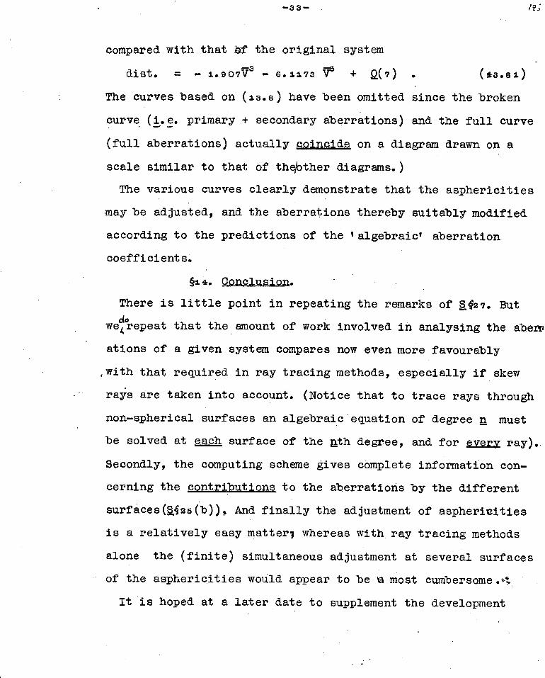
-33-

compared with that bf the original system

diet. = - 1.8071r - 6.1173 V5 2(?) (*3.81)

The curves based on (13.8) have been omitted since the broken

curve (i.e. primary + secondary aberrations) and the full curve . —

(full aberrations) actually coincide on a diagram drawn on a

scale similar to that of thqbther diagrams.)

The various curves clearly demonstrate that the asphericities

may be adjusted, and the aberrations thereby suitably modified

according to the predictions of the 'algebraic' aberration

coefficients.

§t4. Conclusion.

There is little point in repeating the remarks of 3427. But do we 4 repeat that the amount of work involved in analysing the &Dery

ations of a given system compares now even more favourably

with that required in ray tracing methods, especially if skew

ran are taken into account. (Notice that to trace rays through

non-spherical surfaces an algebraic equation of degree n must

be solved at each surface of the nth degree, and for every ray).

Secondly, the computing scheme gives complete information con-

cerning the contributions to the aberrations by the different

surfaces(S§25(b)), And finally the adjustment of aspheriuities

is a relatively easy matter; whereas with ray tracing methods

alone the (finite) simultaneous adjustment at several surfaces

of the asphericities would appear to be ka most cumbersome.

It is hoped at a later date to supplement the development

-34-

above with a systematisation of the means of calculating

aberrations of order higher'than the second. In particular

it is hoped to give AIL expressions required for the calculation

toil the complete ItELLILy aberrations explicitly. Certain other

problems may also be dealt with, such as the aberrations of

optical systems with continuously varying refractive index,

which will incidentally throw an interesting light on the math-

ematical foundations of the present algebraic methods.

The following table is to be regarded as a supplement to the

table of a927..it contains the more important new symbols which

occur in the text. The numbers in brackets again refer to the

section In which the symbd1 first occurs.

pymbol

Meaning of symbol

A

a/co . (5 )

ai (i=o,...,2) coefficient of Y iV3-1 in el ,(Z =W =0) . y

bi (i=o,... 2 5) coefficient of YlVI -i in el ,(Z 1 =W1=0) . (is)

curvature of curve generating refracting SlarfeAW

Q. N(Y — TV) . (2)

N(Y - roV) . (2)

Yi ( 1=1 ,-1'0 groups of terms in J and L . (s)

D . (1=1,2) D = Z a.pi , D= Z b.k . (13) i 1 vIxi 1 2 tat 1

1 Y.V = YV + ZW . (7)

*V-V = V2 + W2 . (9)

Gn coefficient of 9C1 in series expansion of 3. (2)

-35-

unit normal to plane of incidence. (3)

g/kro . (3)

J coefficient of I in AA . (4) '

coefficient of Y in AA . (4)

rf AN . (4)

Y.Y = Y2 + Z2 . (7)

(r - x)/r . (s)

paraxial location of entrance pupil . (13)

z. (2)

ro Zo. (2)

175 . ( 2 ) (ar - giro ) . (2)

a'n coefficient of1G 11 in expansion of Q. (2)

Oamt . (4)

a radial polar coordinate used in specifying rays of a pencil with respect to pr.ray. (13,

- V VI of principal ray. (13)

y2 + z 2 ( 2 )

coordinate of points on surface . (2)

X xS . (4)

angular coordinate corresponding to a . (i3)

coordinate of points on surface. (2)

Y of principal ray. (13)

coordinate of points on surface . (2)

-36—

References.

Buchdahl, H.A. 1946. Proc.Phys.Soc. LVIII. p.54s.

t 1 1947. This thesis, p. 32 .

tt 19 48 . J. O. S. A. V01. 38 NO. 1. p• 14.

Oonrady, A.B. 1929. Applied Optics and Optical Design. O.U. P. Ch.VIII., p.4o6.

Atf.

TUEALMBEAIg__THEDRY cALWILATIoN OF THE GumETRIcAL NIGHER ORDER ABERRATIONS OF OPTICAL SYSTEMS.

III. Supplementary results concerning the aberrations of the general lymmetrical optical system.

by H.A.Buchdahl, Department of Physics, University of Tasmania.

Abstracts - In part I of this supplement a systematization of

the explicit algebraic developments arising from the author's

previous work is carried out. The purpose of this is to make it

possible to derive all expressions necessary for the computation

of the aberrations to any required order according to a definite

systematic procedure. In particular, all expressions necessary

for the computation of the (exact) primary, secondary, and

tertiary aberration coefficients of symmetrical optical systems

are derived in detail by these means. -

Part II deals with symmetrical optical systems in which the

refractive index is a continuously variable function of position.

This is of heuristic interest insofar as eLagrangian' , treatment

of the subject leads to a development which is in all respects

analogous to the author's previous algebraic methods. Higher

order aberrations are again obtainable by iteration.

In Part III a concise proof of the sine relation is given,

first for the case of 'ordinary' symmetrical systems, and this

is then extended to the case of the most general symmetrical

system in which the medium may be both heterogeneous and

anisotropic, the behaviour of systems of the type found in elec-

tron optics thereby being covered.

• I. TAT T E C OF PERT AR HG R ORDER _ • ek.

ABERRATIONS.

§1. Introduction.

In previous papers (auchdahl, 1.948(2), i948(3); hereafter

referred to by the letters a and A respectively) the author has dealt at some length with the general principles underlying his

algebraic methods for the determination of the exact higher

order aberrations of symmetrical optical systems. In particular,

all series expansions necessary for the determination of the

primary and secondary aberrations of such systems were given

fully in explicit form in al620 and 21, and Al§7-to. On the basi(

of these, sample complAtions were actually carried out for the

case of a Cooke Triplet (1.,Sq25 and M12). It is apparent that

it may be desirable in practice at times to compute the tertiary

or even higher order aberration coefficients. We propose there-

fore to consider now a systematization of the means of obtaining

the expansion of AA when going beyond secondary aberrations, as

otherwise one runs the danger of becoming bogged in an unmanage-

able welter of different series and expressions . At the same

time the recurrence of certain groups of terms is made more

obvious, with consequent shortening of computing schemes used

in actual calculations.

In particular the detailed expansion of AA will be extended

to include the tertiary aberrations; and for the case of the

latter the expressions corresponding to those of S.:21 are also

given in full.

—3—

§2. Fundamental sets of terms.

(a) The basic series of a given refracting surface is that

which expresses the shape of its curve of intersection with a

plane containing its axis of revolution, viz.

tp.,1 (2.1)

(The meaning of any symbol not defined here is as given in the

tables of S427 and A§1 ,1.) In virtue of the identity A(7.2),,

may be expressed as a function of C, 11,4 ,

= 5 n) (2.2)

where as before eX,( n) is a homogeneous polynomial of degree n

in E, , the coefftcients of which are now to be thought of

as combinations of the a n of a2(b). Writing for later conven-

ience x (n) = O n , the substitution of (2.2) in (2.3.) yields

(2.3)

In other words, the condition that the polynomials of degree s,

(5=1,2,...), in the expression

Igi f en N 74:ipm (lip.rri ) 2in on } ( 2.11 )

vanish identically implies a recurrence relationfbr the P m.

Similarly we obtain, with R(n) = Y n

( 2 )r)=-1 Since P = (r- x)/r this incidentally gives, with P(n) = pn

41-4 Pn =m13 - on „,=.1 n-mYm

Po = (b) In addition to the two fundamental sets of terms O n and y n

we introduce two further sets o n and T n each of which is again

a homogeneous polynomial of degree n in g l They are

(n z•J.)

-4-

defined by

= - ±c2 i k2(aVfl ) k2T1R + )11 = = (2.61)

:Lan

= - tk2(a2oe 2aori + ) + 2k2 (10e -

+ OCR? - (1 + j)P21 = Ty, .

It is of importance to notice that the an, Tn ,(n >2), are them-

selves expressed in terms of Y m ,pm , that is, in effect, in

terms of 0m , Ym • In fact

=-112k

a = a0ik2 (a0

.11 - + p +

n = a (kV 4 + pn + p ) (n*. 2 ) 1 0 n- n-1

T o = -k ) /2 k

= -'T 0Ck2(aO 2a0l I) 2P1

n = 0[2k2 (a () - TOA k2

- PmPn-m LZ,PmPn-m-s. 5 77 2") *me

,0

(See also §6(b).) If in any term of a Z the lower index exceeds

the upper, that term is to be taken as zero.

3. Solution of the equation for a.

If the expressions (2.61) and (2.62) be now inserted into the

Quadratic equation 6,(6.6) for S , we have at once

( 7 T )32

1,1=4, n For the sake

let

+ 2( C

ajs + TVW.0 "

of convenience

T =ZS n mS n-m

I:IL/ 1+0 = 0 (3.1) 2k'

we write herafter S n for S (n) . Also

• (3.2)

Then (3.0 becomes W 2 2 (Tjtm 20

nSin) + 11-11(t+S) = 0 .

Ar.0 2k (3.3)

Selecting the terms of degree n , we find

So =

1

anq all subsequent S n are obtained from the relation

Z (Tn-mirm + 2 an-rn8m) 14:: (n ) • (3.5) fizto

This equation may be put into a form in which it is more obvious-

ly in the nature of a recurrence relation for the S n by separat-

ing out the terms m=0 and m=n . We thus get

Sn Z trG S r Sm-r 2(T + an-m )Sm o m n-m n-m

+ (2an + T n) .

f4. pxpression for AA.

(a) In A64 it was shown that AA could be exhibited in the form

= JI + LY (4.1)

*here

and = 1.3r0 - Lcu' o with X = xS .

Accordingly we have at once, since 0 0 =0 ,

X(n) = n-mm •

Therefore j(n) _ Bn uot 1,1,03n-m3m

whence L(n) = sT yoY (b) This essentially completes the systematisation of the

method of expansion. We note how in proceeding from order

to order a, gin and yn , and thence an and Tn appear as essentially

'new' terms. But the equations (2.5), (2v), (2.6), (2.6), and

(4.4), (4.5) cleaiy show how groups of terms occurring in the

expressions for orders ( fl may be used in arriving at the terms

of order n. The simplicity of (4.5) also is a great advantage.

6• (3n, Ynt any 'giro for n =

(a) Straightforward calculation as in Af7 easily leads to the

following terms, using

= g - 2e,g1 + (-2e2 g2 1 + @ler + 492) Q.( 6 ) ( 6 ")

Y i = G i g Y 2 = (a 2 G:al)g2 aoatgl

2 Y 3 = (0, 3 +Y(1.00.2 -1- 1914+ 2e:(1 1 )g3 ■ (2a a +sem + 0 2 • 2 1.."" LeN r2 11

92a g2s ct. 2 0, 1 1 0 1

5•2)

15 1 = gi g P2 = g2g2 "" "1" 1(5.3 ) P 3 = 6eie2 g2 T1 48:gri2

[We are using the On, an indifferently at this stage, according

to convenience. They are related by (v.S§2(b))

I. =ç0

82 = + el

e3 = 2 Au + e2u + 285 6 1 1 1 e. =t(a 3 + 5811a2 + 5o8ta 2 + 38,4 + 4081) .

(b) In virtue of (5.1) and (5.2) we at once obtain the p n from

(2.5), Po = pi = -281g

P2 = .41-etal 28:)e 4E4. gn 4 p. = -(yela. + 4910. 1+tcal+ *el)g3 + (74910, 1+120)en

-2 ete; ■ et0.)2 • J

This in turn leads to the second set of fundamental terms,

in virtue of (2.'7), (2.6), yia.

a2

a3

=

=2-1k-11-agg k2a0 n - (1-k2 )d

= t.[(tela1+ 81)e- (tk2a1+ 2e1) gil + elgS1

4 ^3 1 2 = a2 + 4tolai+t-ai+ 491)e- (k20.2+(k2 +7)921a1+12e51 )g2 11 2 f /

3 1

4- 0- e + 4e4 )es + (OaoGi+ 894 )gil'- 4e3 gri 1

(5.6)

j

T = 1=11 (1k2 +3)e e• ( 2 k2Q 0,3)gl a2gSj

= Amc .2 k f a 2k2 + )(;(. 00. 2 + (k2 +424.)(1 21+ 4k2 +2 )931.a. 1 ) g3

42k2 a. 2 + (10k 2 + 11kiv s.

1 1 •••1/40 N a2 m ,...5121 +(as a 4. 4044 N r21

+(2k2a0 + 4 ) gn2 4griq • i 0

CIO

(a) From (2.6) we obtain for the Sn, (n=1 1 2,2) the following

expressionso S

•

= T

•

20 (6.11) 2k

S2 = ToS: 2(T 1 0 1 )S 1 4' (T 2 4- 20 2 ) (6.12)

S s = 2T oS i 52 2(T 2 +02 )S/ -1- 2(T 1+61 )S2

T 1 S1 (T s + 2a3 )

On the other, hand, from (' 1 • 4

= RYA.- u to01) Lt) = Nydv

(4.6) we have

6.21)

P ) = [Y os 2 - :DO is + 2)i 2) = 13 41 2 "I' Yiti(t)

T o = (1-k)/2k

= - 1.1=11 ril+k2 ) 44 - -ui 2k U. 2k2G01 _ .( . _k2)s]

(5.7)

J

= ao[k2(aol - pi +13

(52 = GoLP2, CPt k2 TlYti

0 2 = 0011) 2 11)2 k2 rY21

for n=1 1 2,2

4T64 = 110( t3 1S 2 13 2 6 1 P )3

113) = iTy0Y3 + (Y1 J421 + Y2 JU) .

(b) It will be seen that, in general, we may proceed as follows.

First the I3 n,Y n are computed to the required order, and from

these the pn . The an are then easily determined from (2.7),Ll

which requires only very few multiplications. We could then find

the Tn directly from (2.2). But it may be simpler to use the

identity 2 • •u n + 2(i.-k)an = T tg[2k2a y + 29 - p + k-Z y o o t n-t m n-m-1 • • Z. pm (pn...m+

4"

which follows from (2.7) an ," (2.6), and the right hand side of

which involves neither pn nor Y n . Thus, for n=2,2,

T 2(1-k)0 2 = 4T (e4 - k2 e1 )e 2 0 1 1 1

T 2(1-k)CY = T g2k2 a. +k2 a 2 +(4k2 -6)93a - 896 .1g ( 6.8) 3 3 0 0 2 1 1 1 1

(2k2 4G I -16e51 )n - 4e:*2

The Sn are then found from (e.t2); kihth task may be somewhat

shortened by observing that in 3 3 the combinations S: and

2(T + c) for instance occur already in S. The determination 1 2 of J(n) and L(n) (n=1,2,2) is now not a very lengthy matter. The

L ( n) especially invildve little further calculation.

(c) The forms of a(n), (n=1,2), may not be quite as convenient

as those of M. But when tertiary (or higher) aberrations have

to be computed the posttion is rather different. It is of course

- r2F

possible that a lengthy search might again reveal combinations

of terms which could make actual calculation somewhat shorter

if a were arbitrarily restricted to be, say, < +. But it is

doubtful whether much labour would be saved in the end, and

certainly the great advantage of leaving open the possibility of

systematically proceeding to some higher order should the need

to do so subsequently arise in practice would be last. In any

case, with computing schemes suitably arranged the labour in-

volved in finding A/1 (n) , at any rate for n< 4, is such as to

make.routine computations of this kind quite feasible in practice

The prototype of such schemes may, in a general way, be taken

as that of Sf25(b).

p. Ppherical surfaces.

Spherical surfaces are of particular interest partly because

of their very frequent occurrence in practice, and partly because

it may be desirable to keep the "spherical terms", (i.g. the

terms of AA which survive when we set a.= 0 (lAips.)),separate

in the course of computation, as was done in Al2. Putting a i= 0,

(it), great simplifications naturally arise. Thus the p n are

now given by the series solution of the equation

(3.'+ )x2 - 2(r0 + 71)x + g = o , (7.1)

which yields the recurrence formula for the P n, yja.

Pn = el[( 9 2. 211 )Pn-a. Pm( Pn-m+ t 0n-m-s. ).1 • (7.2)

02

0 3

= 92 g(92 g - 29 111

= 29(eg - 700 2

+

;

)/k

-10—

All the Y n on the other hand vanish identically, whence

Pn = a on S (7.3)

Theao' o/ T aTare unchanged; but for the 0 2 ,a3 we have 1' 1

simply

whilst the T 2 , T 3 now follow most easily from (5.7), 1.2..

T2 = T COVG ''' 0 0 0

T3 = el (elg + 211)T 2 .

The simplicity of these formulae is remarkable; and the calcul-

ation of'the Sn and thence of J (n) is particularly easy. L(n)

of course vanishes identically.

fe. Tertiary increments in explicit form.

(a) The problem of iteration was fully discussed in sgs(a),(b).

For the purpose of setting out a practical computing scheme it

is convenient to have available -the coefficients g m) et)) in /Ay /iv

the expansion S(5.3) of AA on the one hand in terms ds) - pot

and g(g) g (5) (s=i 1 2,...,m), (the determination of which we

have considered above) ; and on the other hand the sums which arise

from them in the course of iteration, ylz,Gvlp ,..., where (v.§.(3.1o0). In g§21 we gave fully the expressions for

(2) the g r., , , (which split up into their respective )2, and

'components'). We now give, in (b), the corresponding express-

ions for the 42, , gip, in full. They are obtained by subst-

ituting (AciAgi +...+6-430i) - ( S i g.W. +0 0. + *6'6 )

( ApyAir.. +Upyi c) + ( s ipyg+. +§.6 pytc2i)

for XL, Vi respectively in the series

AA -` (EgA:" + 511St ) (21X14. 4.•• 20.43:)

LoY1q) ,

(8 2 )

using the notation of S(3.4),(3.1o). Selecting the coefficients

of the terms of the seventh degree then gives rise to the

expressions set out below. The corresponding expressions for

the gl") 9 g ("' (m :4) may be arrived at in a precisely

el rA.V

similar manner.

As before each equation splits up into two components. Soa

that if we are interested in the tertiary aberrations for

arbitrary object position the increments, considered collectively,

consist of the sum of 2.692 = 2.384 separate terms. But the

following very great simplifications should be considered:

(i) the being determined, the ( Fl g follow very easily

by means of relatively zfew multiplications.

(ii)Most of the multiplications are the product of primary

coefficients, two at a time. There are only :_78, such products,

so that many of them must recur several times over. (Also, these

products are rapidly computed in groups of UnaUg, leaving one

factor on the calculating machine during each oalculation of one

such group).

(iii)whole groups of terms recur in different coefficients,

e.g. consider the brackets containing S 2p.

(b) 1tshould be noticed that if N1/ 1 every capital roman

symbol below is to be thought of as divided by N.

CoofTsot

T 3 BAci Ap Ap 12 + (- 3s ici + 3A 2 )1. + (S ip - tAp Ag )L + (S ip - Ag )12.

= + Ap2 k Ap2 2.

Vt + - cyja + Ap 112 + (_ Sig + 2Ag Ag + (61p 2Sig + Ag2 - 7Ap Aq )a

= + (- Ap Aq )b + (Si p + Ap 4p . Ap Acdx +

12 - (4Ag + 68g )i) + Bp + Ckp 4Ag + Bp42 + Ar 12 + 2Ar + lAr 1,1 + (- 2tiq 3S2q + 4Aq Aq + 6Aq BOA + (S2p 2Ap Aq 2Ap Bq 7Aq Bp t

= tp + (Sip + S2p 2Siq- Ap Aq + Aq2 2A-7, Aq 2Ap RC! 2Aq Sp )1i.

+ (Sip - Ap Ag + Ap Ap + 2Ap Bp ( 2S 2Ap 2Ap Ag 1Ap + P

12 - Bg ja + (Bp - 4Ag 4Bq)j1 - .Ag 12 + (2Ap .7.Ag + Bp )A2 + PAID 13 "Lp + (- S2q + 2Aq2 2Aq q 4- 2;-.CCI BO&

• ( • 281g • 2 S2 CI p - 2 -Ap =kg + 2Ag ?gig P0 4 2Ag Bg Bg

+

- 2 + (2Sir 4 S2p . S ig . Ap Aq + Ap Bp a. B g Ag Bp + Ap 2AR ip Ap

• 2Ap icdj. 4 (2s + 4Ap Ap 2Ap Pp )11.

- Fcci cp (CP A'(1 ).§2 (2AP Alq1L3

57 Ap 69 ▪ S3c) Aq2 + 6Aq 7,q )ft + (S3p

• (Sj r - Aq :1 Ao Aq 2Ap Cq COI ( 2Ap 0. AP Aq)b

( 2 1r) + AP2 + 2-AP " 2Aq + (s ID + 2AP AP )Sf

v

Y

= t 3

.01 +

. fel a. “. u ..I or t)

::47. .c1 1 4 Ia.

5 C) I o. cr tr P. . 1I

114 le .4 cr

aft I a. i azi co

co I cn 4 ) +11. Cr

y I c., I cv .44 4 C'! a' I to I ca. 5

I I 44. af cif. a' CJ' ar

cr I - c..1 ...- 1 .4

101 t.;.41. C."

ii. e I I f. 47. P

411. I , 4

I I CV C.. a. p.

4 it, mil 4 cc) co

+ 1,1 .-... 14 Pa cv ...4P C . m

crl

•

p. 1 ,DI cr?' +

.1 ,ar aa al .41' 4 cv I-1 cv 02 01 PP.

+ I P + a.

.4 + cr a' 1,1 c.. ) 4 co

4 ,:r.

a. la) +

t V C:0 P n ' 11 + P.

1 (4-1 co P I a I al ca. S

c I l • e.) 44 9..

.4./4 P. P 4-

n itil ..r al cc 1 :i i 41' 1

cs ■ ne. 1 ell V If a. P. tip

P. ' 4

0' 0'

0' c..) .-.4 4 4 I P. C4r. 0. 4- Gn ..e .

cr. so, i cr.la. • .4 1 crl Cl)i

c-..# oa + os . cr I a ia. la) 1.4 P. I I I P 1 X. i lin r.n .4r i CI.

..-...... .1 P. mu

' Cr' 0' I 4 ci. cr ca cr. Z .1. t... 4 ..4 co -47' s t,r) cm a. P. co + V* 0.1 C11 GU

......... P. P. 1.14 1 + 4 0 ,I C. 45. + co + al co

C-) 4 P. 0" CM ce 1.43. I Co

4 I .--, cs.' C-) 4- Kg

..7. -4 I:. ici,

= 4 Kra:

0' 4.-3 I 5 ialcP 411' c,.2 el c , ....... cfl a. cr ,...,.. cr + ..oi o. r") P. 4 cn I •C + cr cn al -41 .4" I rrI .r. ir ..,sr . -cr + ..,,, I

a. s cr 41. -, ,.. 4 C) c,..., C.) + .0- ca. • V 04 1 4 01 I cc) ■ ..4 cr

4 4a. o I I 01 0, a. cr la, 5 a

.0 c, +41.14 s CU 0'

+I. + • c, .

.45r c

c). c9 e co .0 0

pL. .c.) II si , 1 P. Cr a' a'IC...) I ma. 1 cn ) In. J. .04 I c'tf"' .._. P. ...-..

1 IP ! '5 -4

v) 01 4:7' Cx, 5

c v C'.!4 a. 41' .4. + o' + ....f + i ca a .

+ -4 5 C') a' ' .14 U., 1 4p. 4 i " ial

+ cn c 4 r4 cr • C)' iol Ira i cr v co

(4)'el K .-• m I cr) cv a. icol

.0 c.: 0 r a. c a. 4:r o. a (1•I, CU C'.) V) 0. V) 0.1 01

i gr. AP'

I C/) I 1 C,I II C.' I ..4 5 .4 -4 cn C/) v) ,cv ‘I V*

......... ......... ..... c..„) ..-... '-'- - , c.,4 .._.. ........ ..-...

I 1 I

+ + + 4 + 4 4 -I 4 4 + 4 -4 I.')

44' I .431 144

gt• 41

.2020

.14 Aarl cv

4

a' ■ .01

p. 44 cr. 0'

1 41 1 X p. co

a: 5

II

CO•ff • Of

Yi“ .15 • 1 q + ( Cp • 4 Cg • Ty& + Cp + ( 2Bp • 2ig 3B + 2 Cp + r

+ (2cr, - 2.1)14 + (3ip 2Aq + Bp )15•-.0+- Ap 4Ap AB

+ 38 5q + 4Aq Cq + aq 4Lq Cq + 613_41 Ccds.. _

+ (s5 • 2Ap Cq • 2,1q-- Cr.o•-■2Bp Cq 28q c)

= t5 + (g3p+ 8 5p- 2er 23 Ap Cq + Aqg • Apt qe 2AqCq • ap 2AqCp+ 28p C ci. 2B qC p ).V.qp + S3p + Ap Cp • Ap C q • Ap Al Bp + Cp • Aq Cp + 2B p Cp

+ ( 2 -8- 2p + 233p • S2 q + 2Ap -2Ap Cq + 21p 2Ap Bq + 21Ip _Cp • 2:11rq Cp+ ZBp cp Aq B p )

•

(32p + 2Ap tp + 2Ap Bp + 4Ap Cp 1

V t -

4% ii Cg + (2dp 3Cq q12

-

+ Bg + (3s • 2Aq • 2B + 2C )j.3

• ( 2 Cp • 2 Aq )li + ( • Aq )11p + (4A + Bp Aq )a 5 + 4Ap 16

+ 5q + 4.11q dq + 2Bq Cq + 2Bq Cq )ft

+ 3q • 2 S 5q + S 5p 4- dq 2Ap Cq + 2/1/41 ijg • 2Aq Cq • 2Aq Cp + 2Bq Cci• 2ftpC q• ?NCO,.

= t5

•

3q • Ap Cg + Aq C q + 2Ag + Aq Cq Aq Cp • Bp eq B q Cp

• (2g3p+ S 5r. S-2r33q•ApCr2ApBr2ApCq+7ApCp•liq-Bp•AqCp•211qop+BpCp•BpCq•BqCp+ BC p )1)

• ( • 32q • 2Aq Bp • 2Aq Cp • 2,Ap -fi g • 2Ap COL

+ (332 p + 233p + 4Ap Cp + 6Ap Bp + 4Ap Cp + 2Bp COO

- q.12 + (2Cp 3C q)ft 3 + Cp g3 + (Cp + (4Ap Aq)86 + p 16

• 3S 6q + 21'q 3Sq2 4. (s6p .0 2C p C q)i,

= t6

•

(36p • 3- 3q • Kp d q + Aq q + iq Cq • Aq Cp 2Cp COI + Ap Cq Kg Cp • Cp2 &

+ (2g3p • S 3q PAtp 21 C q • 2Aq ep Cp2)2. + (83p + 2Ap p + 2ip Cp)j.

Coeff. Of

q .2 q .3 P ...3 Aq 15 '' iq 16 + 54p le + (... .. 7 g + (3 .. 2Cq 4 +

+ (-. 2S6q + -§8p + 2Aq eq . 2-CTp Cq + Cq2 )7; z + (gig N - cr Cq )b

= : i

'6 + (S6p - -§3q . 2Ar -eq .2A-q ep + CI) ep .. CD COI + (_ -g3a . 2liq Cr m 2Ar yo

+ (3g-3P + "P (T13 + CP2

)L - —

_

'I 13 ....7 t .. 21-341 12 + (2Bp - 3Bcde4 + Bp 14. + 2Bp • + (- 2S4q 4. 4Rq 4. (..2ti q P ci la

=t7 + (S-4p - 2S431 - Rp 13-q + Be • _113_3) B(db _4.. (S4p + Bp Bp B p B c )b

+ (2Stip + 28p 8o - 2BT) Bcdo + 2Bp2 0

- gig JT2 - 51 3f31::) VOA + 2B n + 214,1 2 a + (- 2S4q + 7,Bq 13q - 2 r'p 4C1

t--4q p 8q + Bq f1.01, + (2 -§4p 541 + -I3p 2 - 2B, Bq - Rp N ib + 29p 1700

+ (234D 4. ?Bp TIPI.

16g

T S te 82 elq 1,3 + (2Cp 3Cq aq )14 + Cp + (3Ep 2Bq + 2c.p 12.5 . + Bp 15

+ 4Bp + 21.5q + 13-q2 + 4Bq Uol + aigq Cq)a + 21q 2Bp )1C

+ (hp g4q 285q Bp + Bq + 213q Cq 2Bq 21Eip Cq Tiq

+ (3 5p + Bp Bp Cq + T3p Cp Bq Cp Bp T3q

+ (234p + 285p S4q + Tip2 + 28p 213p Cq +2ITp Cp 2Bq Cp 2Bq

(84p + 2Bp T3p + 48p COI

V rk` 2eq j — 2Bq 13 — + (3ep 2 Cci 2E04 1.5 (4Wp Pq + 2 Cp

+ 48p + L + 2g5q + T3q2 + 2Bq 2F3p 41. 1T3 q CC1 2 Wq -erdi

= +

▪ ( 2 g - s + 211 - 211p c- - 2T3 T3 213 r — c 5p 441 5q q pq q P q P

+ (•• -§4q rIp 213-q Cp 2Bp -dci )0 + (Ain + 2s sp + 313-p2 + 4tip + 4T3p Cp )g

Yr“ ' 2 q 64 + ( 2 T3q ) 3 Cr, ( 413 Bq + 4 Cp )16 + B

+ 24,q + 21Tq + 4 Cq eq )8. 2Cp Cq

+ (5613 _ s-zeg — 2s6q + Bq "dci Tp 7ci cq - cp "Cc, - 2 Cq CC12

= t9 + (Sep Br q Cp + Cp 'F/3 cp cq ii; + (24p + 2s6p - SRI + 2-Ap 2Fp Cq + 2Cp 2Cp Cq 29q Fr )1

2 , + (S5p + 2B p + 213p Cp + 2Cp Jo-

Cooff. of

✓ 2trq — 2Z4 IA Cq + (4ap gq .1 Cq/16 ja3 ( 514p + 4Cp LSO q2 )5

+ (a. 216(1 2Cq 2a-p ;NT + g6q 21kg Cq eq Cp eq

= r + (2g6p - g5q • S6q • 2rip aq • 2ffq C-p2 • 2 Cq • Cp

▪ r5q 2T4q 2Cp + (asp + 286p + dp + 4C.ro ep )o 4

• Ti 110 - a-q 15 + (4; Cq ).26 Cp ..116 (6q2)11 (-1/6q Cq Cq " C-p

tio + (- Cp Tq)j + 2-16-p - s 6 Cq,p rp2 )2. + (S 6 p 2C p

✓r 5.1 0 - - ;116 + ( q2 )1 + (dq2 )k + (- t.6q - 2ap ;)12.. qJ = tio + (- 8 6q 2 Ccdo + ( 3S6p + 3 -dp2 1.9..

207

49.Conclusion.

In conclusion, rather than repeat the remarks of gs27 and

At§ 14 we take the opportunity of referring to some recent remarks

of T. Smith, (Smith, 1948). It is reasonable to claim that the

methods set out above provide just the algebraic tool for the

examination of higher order aberrations which Mr. Smith wants

to see developed, especially as it provides an easy method for

the control of aberrations by means of manipulation of the

asphericities of refracting surfaces constituting the optical

system.

In complete accordance with his remarks it may be worth while

to examine possible combinations of frequently recurring terms,

as was already pointed out. in 06(c) above, coupled possibly with

the construction of tables of certain functions of t 4 etc.

Finally it may be mentioned that as long as the present

canonical coordinates are used it is not likely that any algebraiA

method can be p_aaantlally shorter than this one. These particular

coordinates were singled out by the author from amongst other

linear coordinates, (v.Sffi2 and 17), bacause they seemed

especially convenient in practical work, and because they are

always allowed coordinates,whatever the properties of the part-

icular optical system. Nonetheless, an investigation of the

advantages of the use of coordinates normally employed in Ham-, ilton's method might prove most useful. For the resultant new

feature would be the great simplicity of the identities between

•19- .2e6

the aberration coefficients as defined above. The problem would

then simply resolve itself into the calculation of the coefficieq

of the power series expansion of one or other of the charact-

eristic functions of Hamilton, by means of an adaptation of

these methods.

For references vide page 46 .(255)

-2 o- 26?

PART II. THE GEOMETRICAL A)BERRATIONS OF OPTTCAL SYSTEMS

WiTaL_OZTIWACTIVE INDEX.

io. Introduction.

(a) The theory of the aberrations of symmetrical optical

systems consisting of a medium with continuously varying refract-

ive index is of considerable heuristic interest. The aberrations

may be obtained by considering such a system as the limiting

case of a system of the type previously considered when the

number of refracting surfaces tends to infinity, (y.119(c)). A

solution of very great simplicity may, however, be obtained

more directly by dealing with the equations of variation

arising from Fermat's principle; that is,by considering the

optical analogue of Lagrange's Equations of analytical dynamics.

The resulting development is in all respects analogous to that

applying to a system of a finite number of refracting surfaces;

a matter which will be more fully dealt with in f19. Here again

it appears that for practical purposes at least these methods

may be preferable to those oP Hamilton. This is perhaps not

altogether surprising. For in a great number of actual problems

of analytical dynamics one naturally attempts a solution by •

means of Lagrange's equations (of the second kind), rather than

by means of the canonical equations of Hamilton. Whereas the

latter are frequently more suited to considerations of a mote

general or abstract kind, (g.g. the existence of algebraic

integrals in the three body problem), they are not always con-

venient in the treatment of more'practical'problemsI and anal-

ogously in optics. Nevertheless it appears that so far the

present subject has generally been dealt with by Hamiltonian

methods, and then only as regards primary aberrations, (git.

Ianeberg, 1944, Oh. V. P.322). rWhere 'Iagrangian' methods have

been used, they have been, in the author's opinion, much

encumbered by the use of cylindrical polar coordihates$

Picht, 1939, and the references given there.) Here, Cartesian

coordinates are used throughout: and nothing prevents us from

deriving higher order dberration,7 coefficients in explicit

form by an iterative process, (m417-18).

It may be added that apart from its heuristic value, the

theory finds immediate applicatiola in connection with the

electrostatic electron optical system (Frank und von Misesi 3.943)

(The electric-magnetic electron optical system may be dealt

with by an extension of the method set out below. But on account

of the anisotropy of the 'medium' the theory will be rather

more complex.)

(b) It will be seen that the following method is really a

special case of a much more general method of aatagalaing_tha certain solution of "'nearly linear" second or higher order equations, or

systems of such equations as series of ascending Dowers at

initial values. The equations are called nearly linear if they

can be regarded as perturbed linear equations, i.e. if the

equations became linear when terms containing higher powers

than the first of the dependent variables are neglected. (The

*-2 2 - 211

perturbing terms must be capable of epansion as series in

ascending powers of the dependent variables and their derivativ0

The equations need not be derivable from a variational principle.

This method of solution is so 'obvious' that one would expect

it to be a standard procedure; nonetheless the author has not

been able to find any references to it in the literature on

differential equations. (It may be noted that it is analogous

to the method of variation of parameters for the determination

of faeparticular integral of a non-homogeneous linear differentia]

equation). However, it would lead too far to consider the

general problem here.

. The'continuausl symmetrical opfical system.

(a) The passage of light rays through an optical system consist. of wlw;civ

ing of an J,sotropic medium the refractive index Nis a function

only (i) of L, (ii) of the perpendicular distance from the

L-axis, (i.e. the axis of symmetry of the system), is governed

by Fermate Principle, in the form

ofIdx = 0 ,

where the Lagrangian L id given by

L = N(g,x)A/1-7777 (11.2)

with g = y2 + z2 yv zw s ‘=, v2 + w2 (11.21)

(x,Y,Z) constitutes an orthogonal Cartesian coordinate system,

whilst V = Yl. Dashes now denote differentiation with respect

to x, unless otterwise stated ; and Clarendon type as usual Indic.

-23-

ates that the symbol represents both the Y and Z components of

the quantity in question. (A table of symbols as used in this

paper is appended in f2o).

Write for the refractive index on the axis

N(0,x) = No (x) (11.3)

Then we may define the " equi-refractive" refractive surfaces

of the system by the equation

No(x) (tt.3t)

where 5-E,Y,Z are current coordinates on such a surface,kith

as origins and over this surface N is constant. As usual we

assume that the equi-refractive surfaces have no singularities

in the vicinity of the 2i-axis. Consequently we may write

N(g,x) = 7 N(x)&' , (11.4) AL

the series on the right being convergent for relevant values of

x and g. We now write

L = ZL =lao +L * , (11.6) t

where Ln is a homogeneous polynomial of degree n in g,c. , mtg.

L = 7 (i)N (x)e-Imen (The arguments of functions will usually be omitted when no

confusion is likely thereby to arise.) In particular

Lo =N0

Ll = Nlg + L2 = N2 g2 + i1070C 2

L3 = N3 g3 + t1T2 g21C ■ tNigo + .

(b) Equation (11.0 gives the variational equations

-24-

(Li a. A- _ o . y, dx aV

If we write itly = 1L1 z = G

this immediately leads to

(N - 2N Y = F . 9.-

4,13

2

f t 2. On the associated linear equation. and q. soIltions.

(a) With (11..7) we associate the self-adjoint homogeneous

linear differential equation

(N 0v)' - 2N y = (12.1)

where v = y , . (.12.11)

•A definite solution of (t2.1) requires the specification of two

boundary conditions. We consider two particular linesAy independ-

ent solutions of (t2.1), corresponding respectively to the

boundary conditions (I) at x=a, y=t v = o

(ii) at x=a, y=o , v = 1 .

We distinguish the two solutions so obtained by the subscripts

p. and a respectively.

(b) Let f(x) be one particular solution of t2.1). Then the

general solution may be written as

y = Af(x) + Bf(x))1if(x1N0(x) 0..3)

a f(x)[A + 133(x)] 2 say, a )] 2

dx

where A and a are constants of integration, and a is a constant. Making use of the boundary conditions (12.2) we find-

yp(x) = f(x)Ae l - N0lflf(x)3(x) (12.41)

yq(x) = N0lflf(x)3(x) , (12.0

-25- 2/V

v (x) = f'(x)/f 1 - Nolf1A10(x)f(x) - Nolcf'(x)J(x) , (12.6)

v (x) = Nolf lAto(x)f(x) + No lf if'(x),T(x) (±2.7)

where the subscript '1' indicates the value of the furtion

at x = a • The Wronskian (gt. EzaKe., 1943, p.72),

lyp(x) yq(x)I N01/140(x) W 0 (±2.8)

Iv(x) vq(x)I

as is necessary if the p and a solutions are to be independent.

Any particular solution of (12.1) may now be exhibited in the

form y(x) = yp(x)yl + yq(x)vi . ( 12.9)

i13. On the solution curves of the linear eouation.

(a) The equation (±2.1.) and its solution (±2.9) completely

govern the paraxial behaviour of the optical system, a particular

solution curve of (±2.9) representing a (tangential) paraxial

ray. Thus consider a particular set of such curves all the

members of which pass through:the point (a,0)1 for these

y = yq(x)vi • (±2.1)

Accordingly id we suppose that one of these curves (v i 0)

again intersects the axis at some point b , b >a , then all of

them do, and b is determined by the condition yq(b) = 0, or,

by (12.6), f(b)J(b) = 0 . ( 13.2)

If we further exclude the uninteresting case that J. possible

solution curves pass through the point (b,0), then we must have

f(b) 0, since otherwise yp(b) = y(b) = O. Hence it follows

that b is the solution of the algebraic equation

J(b) = o . (±9.3)

-26-

We assume hereafter that (13..3) •has a root >a and we shall

generally consider only the first root, if there are several.

The values of functions at x=b will be distinguished by the

subscript 1 2 t

For all curves passing through the tobint (a,y1 )

y(x) = yp(x)yi ya(x)v1 1 (13.4)

where vi is a variable parameter. Hence allIrays'pass through

the point (bap2 y1 ). The (paraxial) magnification of the system

associated with the two conjugate planes x =a,b is therefore

m = yP2 = f2 /f1 (13.6)

(b) It is, of course, not essential that a itself should

determine the position of the object plane. On the contary, let

it be at x = a , and let the conjugate image plane (in the sense

above) be at x = 13. Then it is easily verified that b is

given by the algebraic equation

J- ( •) = 3(;) • (13.6)

dx = 0 . g rx)1 2N0 (x)

For the paraxial magnification associated with these conjugate

planes we then find in virtue of (13.3)

m = Yp( 13)hip( -g) = f( 15)M -6,) • ( 13.7)

Notice that (±2.8), WI.

No(x)rp(x) Yq(x) I = const. = Nol (13.$) v (x) v (x)

constitutes the extension of the Lagrange (Smith-Helmholz)

theorem,for the type of system here being considered.

-27-

0.4. Introduction of 4(x).

(a) After the preliminaries of §§ it-10 we may now turn to the

question of aberrations. Consider the expressicin

A(x) = No(x)(y(x)V(x) - v(x)y(x) .] . (14.1)

We have A' = (Noy)ly + Noyv - (Nov)ty - Novi

In virtue of (11.7) and (12.1) it follows at once that

A' (x) y(x) ji . (14.2)

Integration - from ft to results in

A(x) = A i + y(t)F(t)dt (14.2) a

where F(x) are the functions which result if we substitute in

F the solutions Y(x), V(x) of (ii..?), (supposed known). We thus

arrive at the pair of simultaneous equations

A = -

C1 =NyV- 0

NvY=NV P- 01-4-

Nov =-N y 01 1

+ fy„ ( t)F(t ) dt .- + & t 1E ( t) dt .

These may be solved for Y(x), WO, making use of (2.6). We find

Y(x) = yp(x)Lyt + A(x)) + yg(x)(V1 + 6 (x)]

y(x) = vp(x)[Ys. +(x)] + vq(x)Li. + kv(x)]

where s o(x) = - Iro'lilya(t)F(t)dt

o(x) = + N7J.- pr,(t)F(t)dt .

The second member of (14.6) follows from the first of course

also by simply differentiating the latter. Butting

(14.7)

and integrating by parts, (14.6) becomes

-28-

o(x ) = NoIV Ia - 1‘ .L0i jfax (vc107 + yclif)dt 1(14.8)

ov(x) = - tjypliviifi xa + to; fax(vpftv4 ypg) dt

115. Aberrations in general.

We assume as before that the system produces a real image in

the plane x = b of an object in the plane x = a. Then,

Qinceyolv = 0 , the image height is given by

Y2 = Yp2(Yi. Oy2)

Hence, by (i3.0, Y2 = M(Yi A72) (15.2)

We have therefore for' the aberration mY1 ), by (14.6),

= - 11.A(t)p(t)dt (16.3) a

where (15.50

In virtue of (14.8) this may be rewritten in the form

(15.4) OL* a

since the integrated part vanishes, (y (111. = yq2 = 0). (16.4) may

also be written as

s = yta,- + v t . (15.5 )

a (15.4), or (15.5), together with (2.2.1.) contains the whole story

of the geometrical aberrations of the type of system under

consideration, (for the conjugate planes x = apb).

416. Primary aberration.

(a) The primary aberrations (for the conjugate planes x = apb)

follow directly from (16.5) if we take

L* ri L2 = N2 e Ef NoV (18.1)

(Arbitrary planes of references may of course easily be dealt

with). (16.5.) gives . b

+ N IS )Y + va(Ntg - 12- N0 )t , (16.2) a cl 2

where Y, V, g t c have their paraxial forms, 1.a.

Y = yp(x); + y(x)V1 , etc. (16.21)

The expression (16.2) represents the, complete monochromatic

primary aberrations of the system, and may be used for 'practical

purposes as it stands by carrying out the integrations necessary

for the determination of the coefficients of Y11,..., !j1 .

If we write, for convenience,

P1 = 4N24 / P2 = N1 Yl5P2 2 P3 = "' § NOVP4 1 and. p = yci/ yp 1 q = vq/ vp P

we obtain by inspection

= r tylgl + r 2 yl gi + r 3yill + r 4(2v1i + y1( 1 ) + r 5M 1 u63:

r a. = — p. OpP a. •+ (p + q)P2 + qP3 1dt r2 = ... Cip 2 p 1 .4. (p2+ (12 )1,2 + q2."31 r j dt

r 3 =: -2p, ifip2 Pi + 2pqP2 + q2 P3idt 4.t.

r 4 = - 11 I lp3 P1 + pq(p + q)P2 + q3P3] dt

r 5 = - p.1

4tp4P1 + 2p2 q2 P2 + q4P3 dt . , Considering 2r 2 - r 3 , we obtain

b 2 2ra, ,- 115 = —21113( p - q)1 Pzdt

a = _21 !21_40$ dt

r" gni) by (12.8) 1 where 07' = fb ( 2N /N2 )dt (16.81)

so that we would normally calculate r3 from r2 by means of

r3 = 2r2 + pso2 ion ( 16.52 )

where

PN20 (ie. 5 )

(b) In place of the equation (le.e) for s, one may use

a form of s very usual in connection with 'discontinuous'

systems. It is derived from (te.$) by introducing 'entrance-

pupil coordinates' T, * defined by

= TCOS * + sY1 (16.0

W = Tsin* I

1

where is a certain constant defining the position of the

•entrance pupil. (The object point lies in the tangential plane).

We then immediately obtain the aberrations in the usual norm

Sy = aiT3 cos* + a2T 2 (2 + COS2*) (303 + a4)Tcos* + as 16.7)

sz = alT 3 sin* + a2T 2 s1n2* + ( as + cy4 )Tsin*

with

a2 = (r4+ a 5 )Y1

0 3 = (tr 3 + 2S1' 4+ sq' s )yl

=, no72 u 21-""01w-"1

= s(r 2+ r 3 ) + 3s2r 4+ ersi/T .

). (16.8 )

(c) (16.8) shows incidentally how the primary aberration

coefficients behave when conside'red as functions of a l that is

of the position of the diaphragm,

(5 1/4s = 9a4/Ps = 0

?a2/ s = at;

/O s4b = 202;

aids = (eas + 0 4); .

a = 5 1

It will be seen that §§ 15 and le constitute the direct analogue

of the usual Seidel theory of the primary aberrations.

-3 1- 14i7

aberrations of higher order. Iteration.

Equation (16.8) allows of the determination of the aberrations

of any order by means of an iterative process. The latter corr-

esponds very closely to that described in Sfs. Thus, from (±4.3)

x gr.x we have A(x) - A l= - [A:41x + + vy")dt . (1.7.1)

0- a a "Pc, so that the 'p' and , q1 parts of this equation are essentially

the increments (14.$). If on the right ‘hand. side of (17.4 we

now substitute for L* explicitly from (11.5a), and then put

Y(t) = yp (t)Yi + yg(t)V1 and V(t) = vp(t)Y1 + vq(t)V1 we

obtain what was previously called a 'partial expansion', but this

time of the increments themselves. That is, (17.0 corresponds

exactly to the sum,(2:a45(a)),

Z AA (17.2.) - °Ern i -J

where r nt i is given by S(5.21). Omitting from (17.0 all terms

Q(5) we are left with the correct primary terms of the increments

(When these have been obtained we have effectively the primary

aberration coefficients for arbitrary positions of the object).

Next, take (17.0 with L* = L2 4* L3 . Make the substitutions

Y + o(t) - -y

1(17.3) .§..v(t)

(the increments being correct as regards first order terms), and

omit all terms Q.(7). This leaves us with the correct primary

and secondary aberration coefficients, for arbitray object

position. The way in which the tertiary, quaternary,... coeff-

icients are to be obtained is now obvious, (Note that at each

step we need of course only _determine the terms of the corresp-

-32-

onding order, all earlier terms remaining unchanged). If we

proceed up toorder n,Eay, we may at the last step use equation

(15.5), if the object position be fixed. We thereby avoid one

series of integrations, mi.& those giving the ja!th order terms

in (15.5) with ya, ya replaced by yp , yp .

In practical work one would naturally begin by constructing

'computing schemesisadequate to the problem in hand; and tables

analogous to S(2i.2) may be prepared.

§ia. Pecondarv aberrations.

In this section we briefly consider secondary aberrations, as

a special case of the considerations of the preceding section.

To determine them it is necessary first to find the primary

increments from (14.5). The integrated part, of course, gives no

trouble. Thus consider the expression

[yV(Nlg -N)]/N0 (1E3.0

and write I (x) I P(x) for the integrated parts of -

Then the latter are obtained by making the substitution (17.3)

in (ss.$) and integrating between the limits a and x.

The integrals themselves are not difficult to deal with. In

conformity with (15.4) we define the six integrals

Y o (x) = + 2P2 + P3ldt 01 1 a

y (x) = N-1111oP + ( p + OP' + qPaldt 01

a 2

and Y 2 (x),..., Y 5 ,(x) similarly, by analogy from (i5..1), 1.g.

-33 Z.2.Z

"( 1 (x) = - (aBla ib) ) at , (i=1,...,5). (1.8.8)

m a( b=t Then ô(x) =+I(x) -{Y i (x)Yi gi+Y 2 (x)Vi gi+ Y 3 (x)Yin1 +

• + Y.1 (x)(2113. 74+ X14 1 ) + Y 5 (X)L4

=•Ip (x) -T( 0 (X)XcL gi + Y l (X)(Vi g1 +2Y1 11 1 ) Y 3 (X)IlnI

y 2 (x)Yj l + y 4. (x)ViC i .

Now put L* = I42 + L3 in (15.0. Then

e = - p, f /yclY [1N2 + N + 6N3 2N2 g4 - t1\1. 14 2 a

+ vgyiNig .41704 + N2g2 - + t-NoOlat • (18.)

In the terms of the integrand quadratic in E l 4 we insert the

paraxial solutions for Y(t), I'm; whilst in the terms linear in

we make the substitution (17.3), glImp_Allg_=mgleatiljagg

gvi_Len_h_y_ag,t1. The resulting integral represents the complete

Primary and secondary aberrations of the system, for the con-

jugate planes x = a,b. Separate integrals may again be written

down to obtain e in the form similar to (16.3).

§ 19. On the limitina case of a 1K surface system, as oo.

(a)(1) As was mentioned in the introduction (fio(a)) we may

regard a system with continuously varying refractive index as

the limiting case of a system with h. refracting surfaces, as k-+oo,

where at the same time = 0. [At the risk of creating k-,00 some confusion we have to use the notation of S and. when

dealing with discontinuous systems, and the present -notation

for continuous systems. We use the symbol to stand for

the phrase 'corresponds tot. Thus,

• .?:.!

for any M' )

•••34-

JUN/ A(x)

M j dx dxx

u'--v , etc.

quantities on the right hand side of such 'equations' always

refer to the continuous system.]

(ii) We Obtain the equation of an equi-refractive surface from Do

(1i..21) if we set = (:),Cn (19.2)

in conformity with A(2.2). Thus, expanding N(g,x+2) in a series

of ascending powers of and R.,. we obtain in view of (11..4) for

the first two Ws: 01 = -

is accordingly ro N'AN 0 1 •

Now for the paraxial ray-tracing equations we have

u j .1. 1 = (1-yyj /r0i + k.u. 3

= y. - dtu. JJJ+ 1 But ( -k b ) t (N00 )dx

t dx d"J

U3 +1- ui clx

yi dx

Substituting these in (2.2.22) they become, respectively,

(Nov)' - 2N 2.y = 0

y' - v • = 0

(iii) In the case of the usual expression for Petzval curvature

we find similarly

1(19.21) e2 = (gr2. [—N2 + t(N2a/Nb),] The paraxial radius of curvature of the equi-refractive surface

(19.22)

1 . (19.23)

1 (19.24)

.-35•••

roj 41(1/14 j ).-.4 jr(-NOT)(-2N 1/W0 )dx = .1(2Ni/N20 )dx a a

= cfr p by (i.6.51) • (3.9.26)

(b)(i) The examination of certain non-paraxial equations in

of this context is,some heuristic interest. The 'correspondence'

of the various quantities involved is now somewhat more difficult

to ascertain. The main difficulties arise from the fact that the

two Y 's do not correspond. Considering any point x,Y,Z on

the ray, its slope there is given by V, so that the two V es

correspond, i.a. with the present sign convention

V ■ (t9.31.)

On the other hand the present x,Y clearly specify the coord-

inates of the point of incidence on the particular equi-refract-

ive surface passing through this point. Its polar tangent plane

passes through the axial point x-r , where r is the solution of theequation N0 (x-) = N(,x) . ( 19. 3 2)

Hence with this value of 4 Y 0•0 Y - RV . (19.33)

(ii) Since, by (14.2) At(x) - splits up into two factors, one

of which does not contain paraxial quantities explicitly, such a

splitting up might also be expected to occur if we consider

46 j' =ANi (YiYi uA) 0.9.41)

where 'irj are the coordinates of the points of incidence of the

ray on the 1-th surface. In fact, we have at once, omitting the

subscript 1, i7

since

= yANV - 7yAN/r0

Ay = a = 0

( 19. )

and. ANU (AN)y/ro . (3.9 • 43 )

Also, 7= Y - xV, so that, by A(5.8), this may be put into the

form = y(xANV - , (19.44)

which clearly exhibits its quasi-invariant nature. They of

(14.2) may therefore be regarded as corresponEng to the coeffient

of y in (19.44). tUnfortunately the simplicity of (i9.44) is

adversely overcompensated by the fact that

2i = Wiu'in(x- xj ) o , in general.] (19. 45 )

Not only the paraxial relations but also the aberrations

of the continuous system can be obtained by limiting processes.

Some curious features then emerge. As an example we merely

consider the primary spherical aberration coefficient o i. By

(15.4) this is al = -0N2 471-2Nlyqvq-tNavq)dx . (19.51)

Since in the subsequent development all paraxial quantities

appear with the subscript g we shall consistently suppress the

latter. The spherical aberration of the discontinuous systemon

the other hand l is given by (Buchdahl, 1949(1), equ.(7.2))

al = (i/DlulAN(1-k)yi 2 (i'-u) + 4(N'-N)(92 -91)y* li .0.9.52) i

Inserting in (19.52) the various 'correspondences', (paying due

attention to different sign conventions), it becomes

al a1. = b ;Ni\

_y tElov - 2Nly)2 (2Nbv - 2N01 N'

) Jaud

N N N' N N" N3 + 4N70 ylEa. + ....1....A. .... ....1.._a + .1dx . N' NI 2N' 3 DP 3 0 0 0 0

Multiplying out the various factors we find

01 = pj(1-4112 y4- sN1y2 v2 + Nloyv3+ (8NI/D)y3 v a

(19. 54 )

+ [(4N apt /D110 ) - (2N:Ng/Nlo iyl dx . (1.9.6)

a

Now the fourth, fifth, and sixth terms of the integrand do not

contribute to the integral, for they may be written as

(211 1y4/4)t

(19 . 61)

The intgral of this vanishes at both limits, since y qi=ya2 = 0.

Similarly, fb

.ja N,!) yv3 dx

integrating

= -Ja(Nov4+

= oedx

the third term by parts, we find

6N0yv2 vt)dx

+ 3jb yv (N'ov - 2N2.y)dx , by (12.1). a

The integral on the left is the same as the second integral on

the right. Hence we have

.1 1)Ndx = ja ( tN0v4 + 6N2.y2 v2 )dx a fb

•

Substituting this in (2.9.6) we obtain

(3 1 = p, jb,a 4N2 y4 + 2N1y2 v2 - §Nov”dx

which is identical with (19.61).

The curious feature revealed by, this development is that the

integrand on the right hand side of (2.9.6) (which corresponds

to the usual sup for the primary spherical aberration) is so

complex, especially as regards the appearance of first and second

derivatives of the Nm(x). These are all absent in the final form

(±9.7).' That this is so is explained by the possiblity of

carrying out one general integration by parts in (16.2), yiL

21,* of the term v dt ay together with the vanishing of the

integrated part.(One would have thought that there might be a

corresponding simplification in the expressions of the theory

of discontinuous systems. But this does not appear to be the

case).

(19 .62 )

(19.7)

-38

4 2 O. Conclusion.

The theory outlined above possessnsuch simplicity that it

should be well suited to practical application, e.E. in electron

optics. It is valuable from a didactic view-Point as regards the

light it sheds on theory of systems of refracting surfaces, as

well as in respect of of its directness in the application of

the differential equationScorresponding to Lagrange's equations

of motion.

It may be objected that little mention has been made of

the convergence of the many power series which occur, or of

the iteration itself. This, however, appears to be a general

fault of optical theories. To the author's knowledge no formal

proof has ever been given that even the simplest series converge,

such as the series for the spherical aberration of a system of

coaxial spherical refracting surfaces, that is, the series the

coefficient of the first term of which is the first Seidel sum

a1 • It is quite possible that it may not be too difficult to

• establish the convergence of such series for continuous systems,

by means of the usual devices of mean value theorems and dominant

series and the convergenue of the corresponding series for

discontinuous systems might then be deducible by using suitable

limiting processes. This, however, must remain a subject for

later investigation.

The following is a list of the more important symbols as used in

this paper. The numbers in brackets again refer to the section

-39-

2ZS

in which the symbol first appears.

=hal Meaning of symbol

a defines the position of the object plane. (12)

defines the position of the image plane. (12)

P coefficients in first order terms of c . (16)

o(x), -lc jr y,Fdt +N -0-11bynEdt • (14) a -1 a

8 - MY . (is) variation4derivative of -11* w.r.to Y . ( ii)

YV + ZW . (11)

variational derivative of -L* w.r.to Z . (11)

V2 + 12 . (10 .

1(x) integrated parts of increments. (1s)

J(x) f)0(x) if(x)1 2.1 1dx . (12)

N(C,x)1A+ C. (11)

Ln n-th . order term of L . (i1)

L - Lo - L1 . (11)

N0 (x)fy(x)2(x) - v(x)y(x)] . (14)

m/Nol • '(16)

N(C,x) refractive index. (±1)

Y2 Z2 ft (11)

Nn(x) coefficient of el in expansion of N(C,x) . (11)

p (subscript) refers to solution fixed by x=a,y=1,v=o . (12)

i quantities occurring in the r integrals. (16) P

Yq/ P • (16)

q (subscripts) refers to solution fixed by x=a l y=o,v=1 . (12)

-40--

auxiliary variable of integration. (14)

V

x,Y,Z

yt . ( 2.2 )

orthogonal Cartesian coordinates. (11)

paraxial Y coordinate. (12)

denotes differentiation with respect to . (ii)

1,2 (subscripts) refer tcr object and image planes respY. (i.2,13)

For references see Dage 46 • CZ35)

-41-

FART III. ON THE SINE RELATION. •

422.. The case of systems of coaxial_gaLLActlng_Aurfacel of revolution.

The sine relation states that if, in the absence of spherical

aberration, a symmetrical optical system forms a well-defined

image h! of an infinitesimal object h situated on the axis of

the system and perpendicularly to it, then for any ray passing

through object and image

Nhsin9 = N'h'sin9 / (2t.t)

where 9, 9' are the inclinations of the ray to the axis in the

object and image space respectively, the object being immersed

in a medium of refractive index N and the image in a medium of

refractive index N'. (. Steward, £928

We propose in this section to give a very simple (algebraic)

proof of (21.0 for the case of a system of coaxial refracting

surfaces of revolution. As was shown in Al2, it follows immed-

iately from elementary consideratipns that for such a system the

quantity K* = N(Ylly - Pliz )

is an optical invariant, so that

NO'Hy PHz) = - WHO ,

where undashed and dashed quantities refer to object and image

space respectivel* throughout. If the system produces a perfect

image,_ H! = mH (21.4)

whare m is the (paraxial) magnification. Hence (21.3) becomes

(NP - mr3t)/H1 = (By - yfix. ( = const. + 0(2)) ,

••■ 42 ••• .2:7)

where the member of this equation in brackets easily follows

• by considering paraxial values of the ratios on the left. Hence,

for infinitesimal H

= mBrt! (21.6)

or, squaring and adding the component equations,

NIV1. - e = mN' (21.7)

But a = cos9 I a' = cos91 , and m = 10/1h (21.6)

Consequently NhainG = N' h' sine'

which is (21.1).

§22. Generalisation of K * .

By a method analogous to that of the preceding section the

relation (21.1) may be established more generally for any

(refracting) system whatever, provided it possesses axial

symmetry. Not only may the refracting medium be heterogeneous

and anisotropic, but it may be such that a ray 'instantaneously'

in a plane containing the axis of symmetry of the system does

not remain in that plane (as in the case of the electric-magnetic

electron optical system). To prove the sine relation in this

case we first derive in this section an expression for the

generalisation of the optical invariant K *

The path of a ray of light through the type of system now

under consideration is governed by Fermat's Principle in the

form oft(g0141x)dx = 0 , (22.1)

where g= y2 4.z2 = yv+ zw 9 47_,v2+w2 and 7 = dx/dx . (22.11)

x,Y,Z constitute an orthogonal Cartesian coordinate system,

the L.-axis coinciding with the axis of symmetry of the optical

system. (The Lagrangian L can always be written as a function

of ,.7-1,4,x . For, by hypothesis, L is invariant with reppect to

the group of rotations which leave the x-axis invariant. Consid-

ering infinitesimal rotations the condition of invariance leads

to a linear first order partial differential equation with four

independent variables Y,Z,V,W, the general solution of which is

an arbitrary function of three arguments which may be takeh to

be C,7)3. The fifth vaniable g. does not enter into the equation.

Hence L may be taken to have the form L( 1 .11,4$x) , where L need

not be capable of expansion in ascending paers of pllao)

The equations of the ray trajectories are

- IL. 0 dx VI/ By

or (y-.Q + - (2y-E4 + vEA) = o dx - in

(22.2)

(22.21)

This may be written in the form

(2VE nL) +Y(A"ax - 2AL) = 0 dx art vg (22.22)

-4-(2AL) +zi-L1 — 2 1IL = o . (IA ac kdX Vg)

Multiplying the first og these by Z and the second by Y and

subtracting vAmiLL a ILL = - z,-v 0 . -"Idk"24 ax P4

But since V = dX/dx this may be written

dx Yw - ZV) -1* = 0 9

which on integration gives

—44-

where

K' a r(YW - ZV) = const.

r 21.1.

(In dynamics equation (22.3) plays the part of an integral of

angular momentum). (22.3) constitutes the desired generalisation

of the earlier K* of equ.(21.2), and reduces to the latter if •

we set ( puchdahl, 1948(4) 9 elu. ( it. 2))

L = x ) A/1-771- . (22.32)

03. The sine relation in the general case.

In view of the result (22.3) we may now derive the sine

relation as in £21. If Y o Z and Yt ,Z , are the 'components of

the object and image' respectively and la is again the paraxial

magnification, then

Y' = m(Ycos* . - Zsin*) I (23.1)

Z' = m(Ysin* + Ycos*)

where * is the angle between object and image (both:, being

supposed 'linear' ). Hence, by (22.3),

r ( YIN - ZV) * mr I( s* - 2sin* )W' - (Ain* + ecos* )114.1 ( 2a. s

+ _ W - ( -V1 sip* + cos*) Therfore (23.3.

When the object height tends to zero, Y --> 0 (112+e=

so that, similarly to the case of (21.3)

rv = ml" (Vtos* + sin* )

rw = ml" sin* +IV cos,) .

Squaring and adding we have now

t an9 = tan' (23.0

7-71f-

This may be given a more interesting form as follows. If

is the refractive index of the'mediumt, then

L = NA/37474 .

Hence r = N/2,11-47T + .

Now Y = 0 $ so that it is useful to write for the axial refract-

ive index N(0,0 1;Ix) = .

• Here 4= tan2 43 , and thus we have

2rtane = sine + bcose . (23.9)

*If we now write hi/h for GL., (23.5) finally becomes

phsine + h(it)cose = pth'sine , + h 1 (1)'cose l , (23.9)

which constitutes the desired generalised sine relation.

■■46 ■••

. References.

Buchdahl , H. A. , i946 Proc.Phys.Soc.,Vol.sa, p. 545.

If 2.9461(1) J.O.S.A., Vol. 38. No.i., p.14.

I t 1948(2) This thesis, page n.

If 2.948(3) This thesis, page 148.

19461(4) This thesis, page 209.

Frank,von MiSeS21943 Die Differentialgleichungen der Physik, Vol.II. Ch.I., p.06.

Kamke, E., 1943 Differentialgleichungen,

Luneberg,R.K., 2.944 Mathematical Theory of Optics, Brown University Lecture Notes.

Picht,J., 2.939 Elektronenoptik.fis 4 and 3o..

Smith,T., 2.948 Proc. Phys. Soc., Vol.eo, p. 303.

Steward G.C., 1928 The Symmetrical Optical System, Cambridge Tract., NO.25.

236

O Eddington's higher order equations of the gravitational field.

By H. A. BUCHDAIII„ B.Sc., A.R.C.S.,

Physics Department. University of Tasmania. (Communicated hv WV' O I E., Ph I).

Received lath January. 1947. Rea.! 17th January, 1947,

Einstein's fundamental equations of the gravitational lieid are

— tgoG Agr' = where T' are the components of the energy tensor and .1 is the cosmical constant. In empty space one

— 19"1-; 0 . 1'21 which may be reduced to

( 3 ) since G = 4A, by contraction of (2). Eddington 1 has slum n (§64), p. 13g) that %% hen the eoe;mological term in (2) is neglected these equations may be derived 1.%. Hamiltonian differentiation with respect to „ of G,

1)0 4.7

Distinguishing Eddington's equations and partgrapha hy the letter we have, by (E 35.3)

g i‘ ggfit6Y„.. (A)

ISo that (2) may be obtained by variation of the integral

j (G -- 2A) —gdr, ( 6 )

i.e. by replacing G in (4) by

A — G — (6.1)

The spherically symmetrical solutinn of 3) tim ■ be written in the form kE 45.5)

d81 = — y dr -- radiP — 7-2 sin' 042 + yilti ( 7 ) with y 1 — 20t/r —

whiere nt is a constant of integration. When A (7) ruellicch to the Schwarzschild solution for which

y =1 — 2m/r (7.1)

(Gin -- .1,060 0

( 4 )

Now Eddington has sug L:estefi Il §11.2. p. I41) that instead ,pf the equations

1)K ilgio —

might have been used, It being some fundament al in variant ot her than G. In particular he considers

G p.G' =-= 9'49 '°!I ' B B (9.:)

K " = a9 "B (9.2)

as I eing the simplest alternative invaiiants; hut on these grounds we should also consider the squale , f the scalar curvature

(9.3)

Eddington shows that the :■ehwarzschild solution (7.1) is also a solution of the alternateequations

IOC (1 (10.1)

1)K"

Ian

and it is easily seen also to be a -olutlon of

1)K" 0 1)g,„

The author now 'considers these and other all er ti v livid 1,1%18 arid shows, amongst other remilts, that in 4-space ere,!/ solution of (:i) also a solution of (10.1) and (10.3), and that those i ilutions of (3) which represent spaces of constant Riemannian curvature arc Mao solutions of (10.2). In particular it is verifiell that (7) ( t% ILL A replaced by a constant of integration a)is not only a solution of 0,0 1 ) and (10.3) but also of (10.2) although the space is not if coustani 1:iemannitot curvature unless In 0. (a) Conaider a small variation of K'.

K' (G.,Gia) If

Gi„ where a is a constant., theit

' K' = a(g ,.,.Sg" ± g" PG„,)

0.(50 - 01"8g ,„ ;

2a8G — a 2 (qPqxf ,,,

abfi

(8)

( 10.2 )

(10.3)

4

111.2)

BrCHDAHL-2

5(, ‘ - 98K' -- K'S k _

2a-.- 66 -,. 404 % _

- 2a16(ti - (JtSvi _ 9) -t AS%

= 2u6(4*— 2a% — 9),

i.e. 61c 2a81{.

Hence the condition 81C , i7 = l lead.: t,, thy ,

0, •

1k hich is satiatied in virtue of the faet that equati-li I to equation (1 1.2). t'onsetitietitl ■

soitstion of (II t• a .4)/tifiuti uJ the fliterfo rt fo eqsPilimt 10. i), where a is to he regarded as a constant of integration.

It is r,f interest to note that when 11 this tesuit do. - not hold

when the dimensional nutulAer is other than fon! . ! hi, ill .1 -pit , of

n(-t we have as before SA',

but no •• v

2,1 9 81; na 4a

2a(80 - (:6

-

Renee. IT I b1( ff.:- 0 it follows that, K of (c .1) is now replacel by K G— (n — 2)0

281{ • ( If 4).4 24 6 \

I Ol(dr - 41. j 6‘ 7 fl it T, 11.3)

whieh will in gener41 tail to :mesh

-hail %lei if v As It particular enSf • of the g(•tiet-al mi•

that (7`, with 1 . (1 2)

(both nu and a I•eing vonstatits of integral ion) i i i ii iii iiifi id (10.1). To conform with Eddinuton's notation wt. mriti.

t A = — 2ui r . ti ( 1 2.1)

where now, of course.Ot dues not denote the cos:Meal ron.t ant

Using. the forni ot the U given -by (V. :is.eil wo• fine!

11 • .2r2!2 2 -4 2r i)•* : (31; 2 21.".\'

• 2 (e' r • ' 1, 1 14 :.

Here - • 't 1"ttl.1, flIsh doTtn.te , ditferetitiathm with respect to r. and wr have it - since it tifit neee. - arv to consider variations friim t hi nutlet rical C(171(liti, It

t - r■ ing t 12 1) after the various part 1I i..t.ereviiiitions 11.,%1. I *eh 'performed. we find, following riii'litf(q., ■ 11.1 1 .111 Is ,;

algebraic work, that

— pe4- 2e - P4-0i(x— p');r --I 2 (f BA ) /2 = 4(t -

2r) -- ( \ i.•) 3 ,.')

r 2 (el— 1) r( = 4ar 6am - ■ 1 r3 ,

0,

-OW - T41, 2a2r2 ,

ear —' e - • If/ (r2 (21, — A') + 2r) r()' -- .1'1 (1.' Or

(31/— - 2 (e — 1)/r — 4ar 1 lam -t I II" •1 -1'

= e ..'9` • 4. 2r2i2 r(1' — A') eit 1

4 a mr " 4 71 (CT .

If thes.e values are substituted in the e. xpressions for t derivatives

oviA d _d2 E.)1{ ' cA dr FIA' t

d i:1{ 1 .12 (It ' v' dr2

Lagrange

they will be found to vanish identically. (b) Unfortunately it does not appear poshii)I• to deal with K" th manner above by using equation (11). I ;lit a soinei% hat more s'peeialised 'result 'May be obtained by considering spaces ol comtant I: leflifili OHM

eurvature 2. \ ■ e therefore replace (11) by the equation

Bprop = !,ct (9/4 ,p (14 ) Contracting for a and p (11) is seen 1:U be satisfied. Then

SK". B„,,,e8Bily°0 a

ne ..p — 9 Y OW 7" (frr'' irr /1,„.„

— (go. go,. i , 0,d (!e'gq" - g'Y'P)

&ince (g,„.g.„ — g„,g,„) B.-1" - .1

RUCIMATTL-3

B'fr'• being anti-syininetrical in , and a Aq it iz also anti-symmetrical in p and p we get

SIC - (46G — 4G07Sg — 3

— I rL2 (9789,,,+ g .8g- ) = (alt5G.

Hence SIC - fib gAl; 2aSA

4. (1(661 0011 2(16% . —Ti);

. • . 1)1{ . (161 5)

Therefore, as in the ease of (11.1) we conclude that any $oltstion of (11) defining the line-tlenseni of spurs of -otistanl Riemunn Ian curvature is also a ao;uiion of the altfrnutire eguu'ions (10.2).

Now (7) reduces to the de Sitter line-element ( 70.1) when us 0. and the latter defines a space •)f constant kietnNtinilin cur- vature. Hence we know now that (10.2) is satisfied bv the two particular solutions

y = I -- 2no r, and y —

It is natural to enquire therefore whether (12) as it stands may not prihavs also be si solution of (10.2). I y direct suhstitntinn in the equations following (E 62.6) this iiin actually be verified to be the oase. Thus using ( 12.1) again we find

lc 16m 8a 72m 2 + 4(1272,

rs r4 8ar 241/. 2 4a2r4 4ri

eA' r2 3 r3

0, ?A'

i4H' 24m 2 , r. 3

H' Stn 8ar 40m= 20anl 20a2r3 r2 3 r3 3 9

tar' 16m2 leantr 4a1r4 :1

With these values we find that the Lai:range dert.atiAts p{'), vanish identically. Hence

(12) is (11 , t, s(:n ;oh 0.1 the ultcracs;ivc fquations 1141.2).

'Comparing (13.1 and (16) we notice that when ta =

(16. 1)

lit D. t4s 1/C1;. [Hi

tis is required by (11.1) and (15h viz.

olj" 61('

As in the case of K the result estai,lished above (for a *0) again requires the space to be four dim( usional. The equation analogous

+ 2a= —4) . • 810/1- to (11.3) is (it —

gd r

(c) it is scarcely necessary to consider the case ( l0.3) in detail. It will be sufficient to quote the result that, assutning`( ,

81Cudr - -- 4) j 6 . Trir

Hence when n = 4 die result slatfil for K' apply her also. lt may be remarked that 1{"' is identical with %Veyl's action

dersitv (E 90. p. 209) in the absence of electromagnetic - fields (d) The three altetnative fundamental invariants which have been (.01),:i".^-cd so far have in common the property of being gnadratie the r - ceond deri v es of the g,„.. It is of interest to examine wht - ther he results established would also follow for more complex invariants.

Consider for example .ihe a# power . of the Realar curvature is 4-dimensional spacjec... ,

Then 8K(''') inG"' - '8G m (4a)" -18r/ = q8/0 '48% — •

in(4a) - (84$ - G8‘' (40°8V:7.9-

/n(40"G - 18 (0 4(m1.1. 1) a vi g).

Hence f •rT 0 is consistent with I I 2) only if m = 2. i.e. in the

. ease dc-alt itht above. In particular we conclude that (12), (q,.* 0). is not a solution of I K.‘" ?:, --- 0. except in that ease. The author ha, eonsith red various other invari trite involving 3rd, 4th,... powers of the second derivatives of the y„. and these yielded simil'. results.

REFEItENtl.S. 1.:14111•...q4.11. 19: 41 no- Mg , . , csivit 'eta The ,r-y 271.1 rib). 1'.1 . Eu.enhart. 1 1.126. /: , .-wornnegt,, is. 33. Print. .ii 1 .1'

(17)

(17.1)

11(11•Inwor- -

(1271

THE HAM I LTON IAN D El{ I VAT I V ES OF A ( 'LASS OF FUN DAM ENT A L INVARIANTS

By H. A. RU(H 1)A H I, (Hamtd)

[Received 27 August 19471

1. THE Hamiltonian derivatives of fundamental invariants play a prominent part in the Theory of Relativity* since they are sym-metrical fundamental tensoN the divergence of which vanishes identically. In the present paper I consider the class of fundamental invariants which contain the derivatives of the gin, only up to the second order. In particular I shall establish amongst other results the following explicit formula tin. the Hamiltonian derivative h K of such an invariant K

hK — = ZPv°P;„p — f P.440p zr"P +Iry K , (1.1) hg in, where DivaP is the tensor eK/bg„,p symmetrical in p. v and in a, p, as may generally be determined by inspection when the form of K is known explicitly. Subscripts after a comma or a semicolon denote ordinary and covariant differentiation respectively, whilst the order of the subscripts of the covariant curvature tensor I i in,„p is indicated in (4.3) below. We can then verify directly that the divergence of the right-hand side of (1.1) vanishes identically; and the derivation of the Hamiltonian derivatives of various specific invariants is a matter of ease.

2. Since, by hypothesis. K contains the derivatives of the gp., only up to the second order, it follows from a well-known result of the calculus of variations that

Ie(yit- L. i ily _It" ) ± i 2 i (y K ) i (

, 1 2.1) r ( h9p. Vt., ex. g E.f expegi e . _ IIV,01 .. 1 „. 0 1

where y is written for ‘ ( --y). Now, if 0(K) is an arbitrary function of K (satisfying such condi-

tions of continuity and differentiability as are implied in the following argument), then WO is itself a fundamental invariant: and its Hamiltonian derivative is given by (2.1) if K be replaced by MA).

Write = dO(K) = cild(K) O' tr dK ' Ms ' • * Eddington (1), 61, ff.

A822

02 H. A. BUCHDAHL

and so on. Then from (2.1) we have

14(9(10) ig0 ,0+8,VIC K ±

logs. Lego ,. Y + I OK \ +4,4 OK lid

W4v41 449 V 0g*r•001.0 agwv1,0

- 1- 111 - 1c, OK +K.8 °K +2K.(—°K 1+ 2Y.OK. °K 1+ °gProg Npv.a0 gp.r.41 Y 41pw40.1

• (2:2) Ogp;,as

130v is then given by (2.2) if we choose 0(K). K; i.e.

= bK P K ,

'991,v kNoKJA V egor.ct +( + 27. ,, + 1 , OK

g ',YAP! Y p/.3 ( o r,a19 Now the right-hand side of (2.2) is a tensor. Since to( K ) is an arbitrary function of its argument,

Ogpv,4 ZihvaP= =Zv;1 43 .

In the same way the coefficient of 0" in (2.3), i.e. OK a 2y ,

—K +A DAvaLt9 +2K . .ZiAviP.s+ r A —2 a, Z0PciP (2.5)

' 0 „ .. •

But

K a = = K.,.p±{043,a)K ;., (2.6)

Y,p/Y = {fri;cr}, (2.61)- and

frvai$43 = Dare4341 —tal3, p}Za"il —{a. v} Z14° 1 13 — tap, .3,}z1s.us it ag• PI ZI"l° •

(2.62)

:27

•

OK i• OK Nprogii °g#.41:10

must be a tensor. Hence OK , which is symmetrical in a, 11 (and

in p„ v) is a tensor. We. write

OK = DDT'S, (2.4)

is a tensor.

• ON HAN! I I.T ■ )NI N DERIVATIVES 03

Subs!ituting in (2.5). using (2.-II ). and elianging dummy indices we get

C &rail + 2K ZPvcill;s - -

01'

— K:a(— + gap, p}Zwqm + 49, v;ZIA°Pc, + {up, a)Z$ 1 "). (2.7) bgp,.

Hence the quantity

1:ZiAvaP (2.8) cgi•Ket

is a tensor.

3. Now without loss of generality we may for the time being (§§3-7) restrict ourselves to the case in which K has the form

• K = B vacs Ps' (3.1)

where r' ••'- is a tensor of rank 4m made up entirely of the product. of 2m components of the metrical tensor. For the most general second-order invariant is of the form

K , F(K K2 ....), (3.1 ) where F is some function of the tiv each of the latter being of' the form (3.1). When the Hamiltonian derivatives of these are known. that of K follows at once, and is given by (1.1). (as is seen in §8).

Fundamental relative invariants may also be dealt with by the present method. These are formed in a 17 with the help of the numerical tensor densities EP-Iti*--P. and e I() 25J. How t del er-mine their Hamiltonian derivatives is best illustrated by a iiiipIe

example. Let 2 and suppose that the Hamiltonian derivative of

= Owe"' pr (/ap) (3.2)

be required. Raising the subscripts is and p. we get. (3.3) —EtwePg„.

But twPgrots fog, 1(3) 5. (3•43)1• (3.31)

Hence = (tlA ae cto (1, (4) - - y‘ (ttp° 6/1.1 ). where 8P° is a generalized Kronecker delta. Therefore '

K R/y = 002 --(.6,(PP), (3.4)

which is of the form (3.10, Cther relative invariants may be dealt with in an exactly similar way.

A823 •

04 11. A. BU(HDAHL

4. Consider a small variation of K in %% hich the golP are not varied. From (3.1) we have. since involves only the giAv,

SK = LIP"'P 8B (r) Pop' r-1

(4.1)

Ao.s-

where ni

l'Pl tiAvaPM. • B . -1

(4.2)

the dash indicating that, in forming the product. the term s = r is to be omitted. But

BilvaP = ILIWP + gaP•liv -- glw•PP — g PP•140)-4- ft"' ' a q-CrP• — • PP. 1. (4.3)

so that it is at once apparent from (4.1) that all the terms of e K have three -index symbols; as factors. Hence. by (2.8), all the terms of l'iirct have three-index symbols as factors. But YPv. is a tensor, and therefore it must he a zero tensor. Hence

OK = 2(ap, IA} Z"I" — 2{ap, v} Zt`aP - rap, Z"P. (4.4) 1.4r,at

The coefficient of fr is accordingly simply

ZoLve0+ 2/c, Zi'va0;13 . (4.5)

5. In re-expressing PPP as given by (2.3) it is unnecessary to write down explicitly those terms which are multiplied by three-index symbols, for such terms cannot by themselves form the components of a tensor, [(1) 79] and we shall therefore represent them merely • by dots. (This procedure is equivalent to using geodesic coordinates.)

Now, by (2.61) and (2.62), we have

and

7,0 = (5.1)

ZPvciO.cts ZP"0.13= (Zi4v°10:p) ., — {a/3, ft}, Zav — tap, top, tx) . „ Zsv°P-- faf3, Pi.. &Fla (5.21)

(ZPvrci343 ).1 =

Also write [OK/egw,] for the 'tensor part' of OK I,gw„ i.e. for those terms of aKregi„ which form the components of a tensor, so that

(5.22) egg. Lqpiri

ON HAMILTONIAN DERIVATIVES 06

Using (2.4), (2.41) and substituting (5.1), (5.21) and (5.22) in (2.3) we reduce the latter to

aK K +[— ] -1- Z ;c4+ fop, tt),„ZvaPl-f- 1 t ap. v . °got/

(5.3)

6. From (3.1) we see, as in § 7, that ZP1' 343 arises from an expression of the form

214"P ( 1591.11,,ap+ g exit', 89 }tam., 8g rp.i.hcr)' where zPv°P is a tensor.

On changing dummy indices (6.1) becomes

(zPv°P+ z"1"— z"" — zi"")&gpv.ap (saY ). (.I I) ZIAY" is therefore the part of 1,"P"P which is symmetrieill in i t and in a, p, i.e.

bavap l(pvcrp ± 0Aup m 'Cprpo _“vtipo) .

From (6.11) and (6.2) it may be verified that, in addition to (2.41). Zw°P satisfies the cyclic identity

ZP v" ZihaPv ZiiPv° O.

Hence {ap,p}. .(ZvaPI ZrP°.+ Zv..P) - U.

i.e., by (2.41),

2{up, 14 . „ Z"P CI — ZylaPlap, 11; . ,„

Z"°P(Bovir +(a*, 11)„,) r

.-1- — Zwlap. ii} . „ 4

Hence (op, pl .„ Z"P c = IZPA0P11) ,ap +....

Since PPP is a tensor, we have therefore from (5.3) that

PI" = ZihvaP [

;p

OK 1-1- Iry / i(Zv 1°P BP. „0 -s- ZPauP „p ). (6.4) o hn

-wPv The last part of (6.4) may be rewritten in a useful form as follows. Consider the tensor ?As ZiAvar'13A,,,,p . By (6.2) this may be written. after some changes in dummy indices. as

= it(" PlAr )( B Ar, p — BAlvib+ BA,,p,, BA,rd

(2"aP +ZIP1 )(B Arcrp— Br t- BAtpu

(6.1)

from which, in view of the symmetry properties of the curvature

IBA ap (VhvaP -, -Z -r Pa taPihv -f-eavP). y (6.5)

06 H. A. BITCHDAHL

tensor, and after some further changes in dummy indices, we find that

Therefore

13#1v = ZPv°P;op+ -OK

- - key K

± it BY acp (ZP 1°P ± Z aPP° 2 °1101° -f-ZP°°49+ ▪ $14. map(e 10p + ;:..11110 zOprOl zp470W)} . (6 . 6)

7(a). If we examine (3.1), e may think of K written formally as the prodget of in of the components of the curvature tensor with all the indices paired so that to every superscript there corresponds one and only one subscript. Then corresponding to each such pair of indices there is one fact or gaP in In forming SK this 'contri-butes' —gaPer8gpv . So that, if in turn each superscript is replaced by p„ whilst the corresponding subscript is first raised and then replaced by v, and all 2m tensors so obtained are added, then the symmetrical part of the 811111 is —[eKlego.].

(b) Comparing (4.1) and (6.1) we see at once that

ZIA") = ilt14°P

Hence the first four of the last eight terms of (6.6), say er, are in d_tsr

glAP I (Lag') B1.. mop ± I B ay. 01, + B p%-i- r-1

(7.1)

(7.2)

Inspection of (7.2) shows at once that —4er is formed by exactly the same process as that described in §7(a), if we notice that each component of the curvature tensor is now taken twice over, which cancels the factor on the right-hand side of (7.1). Now, where a superscript was replaced by the first time, it is replaced by v the second time. It follows that er is symmetrical, so that

ev qvp —11-1 OK -1-4ZviaP agijr

Hence (6.4) becomes

ZiAvaP iZv 1°P BP ,ap K

(7.3)

which establishes (1.1) for the case in which K has t he ff Inn (3.1 A simple formula may be derived in this cast. fur t he scalar

ON HAMILTONIAN DERIVATIVES 07

invariant P go. P. From the law of formation of [01(140,] given in §7 (a) it follows at once that

gov i OK I 2mK. (7.5) Lagpv.1

Hence. with (7.3), (7.4) easily yields

P (g ZialiP) ;ap + ( fn — te)K. (7.6)

When m in, we see that P has necessarily the form of a divergenoe.

8. I now show that (7.4) holds in the general case when K has the form (3.11). Write

F i'2 F etc.

OK; Also let pavap

'dglAP•al) Then using the summation convention also for roman indices it is not difficult to show after the manner of §§2, 4 that

hK = = ler F f — Ow' K hg pp

-1-fiA(Ki );ap ZiraP+2(KA.ZrP4,11-fijk(K j ) ;„(Kk ): ,, Zi: P°P. (8.1 )

Now consider (7.4) with K F. We have

ZPv°9= fl ZrP. Therefore

PP P = (f Dtv°P);„p

BUt ziraq„„ =f zrP,G +f,j(k);‘, zruP. et e. Hence comparing (8.2) and (8.1) we see that (7.4) applies %% heti K has the general form (3.11). This completes the proof.

9. It is scarcely worth while verifying in full detail that the divergence of (7.4) vanishes identically. I shall merely outline a proof for the case in which K is of the form (3.1). We have

= ZmvaP,„p ,, - (9.1)

If we add to ZPP°P;apv the expressions DAP°P,p and DA"P„ap . both of which may be re-expressed in terms of ZP"P;ap ., by means of the Ricci's identity, we obtain

3ZPv°P ;ap, = 21-1i.A p„ Ziv°P (9.2) :a•

hKi v

A825

08 H. A. BUCHDAHL

all other terms vanishing on account ot the symmetry properties of DivaP and 13. and of (par. For the same reason, when we substitute (9.2) in (9.1). the latter can be reduced to

Bi! ciap:v &etc° 4-1C44 • (9.3)

From (3.1). (4.1) and (7.1) we have at once that

Z$PB, IW J. (9.4)

If the first term of (9.3) be now rewritten in terms of zPv°P, which can be done by inspection of (6.4) and (6.6), it is not difficult to show by applying the Bianchi identity to the resulting expression that it just cancels the second term, so that

0. (9.5)

10. I shall now consider a few examples of specific invariants K.

(i) K = G (= ergaPBomp ). (10.1)

By inspection zi"P =-- 4gPvg°1', giving ZproP = (gPvg°P — igPcfp — igPP9P0 ).

Therefore, at once, since here ZihvaP vanishes, hG (10.2)

nvio, (ii) K = 02 = Km (say). (10.3) It is easiest to use (8.2) with F = Kt; K 1 = G. It follows imme-

diately that hOl • P'")-• = = —2{G4r-FGGiar—gor ( 0 iGI )). (10.4 )

"VpIP

[The symbol 0 before any expression (...) represents the operation gelq•••);crp]•

(iii) K = O,L,0ir = K' (say). ( 10.5) For a small variation of the gp„op alone

SK' = 2G4w800, = 20PVP8B0,00 , 80 that ZP"P --= roCii", and

Davy= g" G+ gaPOPP —ifroGrP— igooGPP— ifrOGva — irpapa.

Using the identities of Ricci and Bianchi we find L GP — O;Pv — 13Vi; +OPPGro -f- 4rvr2.

Also ZP"P „p 134-8.•fGapi-GtoPop.

Therefore

= isK" Pk" hgav

= 4{Litelf" I.P. ‘7.1PG op t- kyPi 1. (10.8)

•

ON HAMILTONIAN DERIVATIVES 00

Therefore AK'

= ClaP P

(;4"

"'71.) ".„ 1 Y""( 1-3 G -T-00"). 'Wow

(10.ti) (iv)

K = B BPv°P - K" (say). (10.7)

By inspection. ZP"P = B"". in view of the symmetry properties of B up. gives

ZP"P = BilvaP BisePa ) . . . . . . . . • Hence ZP"P = 4 Ci Gif" -- 2044 v — 4BP"3PG 4GP°G 1 o.

Again, in view of the symmetry properties of the curvature tensor

ZP"PB%,„0 = 2(110".. a. P. B%,0p ± )

11. In the ease of the three invariants K". Ki", we have in 2 so that, according to (7.6), their contracted Hamiltonian derivative's

Ps, P" must each have the form of a divergence in a I. In fact we find = = _-= (111 )

It will be noticed that the terms involving the tinarth derivative's of the g be eliminated between the three Hamilt MIMI deriva-tives (10.4), (10.6), and (10.8). Thus, if we write

LPv 261/AgG:-- 2 ffrvaP op

L 4K ' + (II .2)

1 AL —

2 hypr

' Ir y L. ( ( 1.3) we have

Accordingly there exists in a V. (n > 4, see below) a linear combina-tion with constant coefficients of the throe invariants K'. K", . namely L. such that its Hamiltonian derivative is a tensor of the second differential order. This naturally implies a considerable restriction on any common integrals which the three sets of ditferen tial equations

PP P 0, PP" = 0, 1:1"' JAP = 0 (11.4)

A826

010 ON HAN! crox IAN DEttIvATIVES

may possess. for they must satisfy the set of suroud-order equations Lsv (11.5) i

It has been shown by Lanczos (2) that hL/hgo , vanishes identically in a I. The same result holds in a I and a I rs .

REFERENCES I. Eddington, The Mathematical Theory of Relativity (2nd e(ln. Cambridge,

1930). 2. Lanczoa, Annals of Moth. (2) 39 (1938), 842. 3. Veblen, Invariants of Quadratic Differential Forms (Cambridge Tract 24,

1927).

PS)

•

4

This article has been removed for copyright or proprietary

reasons.

It has been published as: Buchdahl, H. A., 1948. A special class of solutions of the equations of the gravitational field arising from certain gauge-invariant action principles, Proceedings of the National Academy of Sciences, 34(2), 66-68

UBER DIE VARIATIONSABLEITUNG VON FUNDAMENTALINVARIANTEN

4 "ardiakag--2Q012 RDNUNG.

von H.A. Buchdahl, Physics Department, University of Tasmania.

§1. Es sei K eine Fundamentalinvariante, in welcher die Ableitun-

gen der Komponenten des metrischen Tensors g ttrbis zur (±L)-ten

Ordnung vorkommen, wobei irgendeine positive ganze Zahl oder

Null 1st. Dann ist die Variationsableitung Pt"' von K durch die

Gleichung 611CdT ofK d‘c =-- •Nr-g- dfc (1.1)

definiert, wobei vorausgesetzt wird, dass alle Variationen der

g , und ihrer Ableitungen an der Grenze des betrachteten Inte-

grationsgebietes versc4winden. Ilte v 1st selbstverstgndlich emn

kontravarianter symmettischer Fundamentaltensor, der die Eigen-

schaft besitzt, dass seine Divergenz identisch verschwindet.

(Eddinaton, 1930,

Indem wir die Schreibweise von Schouten (Schouten, 1924, a. 25

und 31) fill- den synnetrischen oder den alternierenden Tell eines

Tensors verwenden, wollen wir nun zeigen, dass Bich die Varia-

tionsableitung Pr"' in einer einfachen Form darstellen lgsst, die

einerseits ihren Tensorcharakter klar erkennen lgsst, und die

sich andererseits zu ihrer Berechnung eignet, wenn K explizit

gegeben 1st. Das zu beweisende Ergebnis lgsst sich dann in die

Polgende Gestalt bringen

P t4V Wifrescre 't1130.4„eX Y)biCre WV K (T e(t") .. T IP"E )j e + (1.2)

Dabei sind die Tensoren X" (re' T4Pr aufgebaut aus dem

KrUmmungstensor ;Lyre. und semen kovarianten Ableitungen, und

den Tensoren E ' r •• .(rj. = 2B0.1 (L. 3 )

und ihren kovarianten Ableitungen.

Steht em n unterer Index hinter einem Komma,so bedeutet er

gewohnliche Differentiation, steht er hinter einem Semikolon,

so bedeutet er kovariante Differentiation. Die Symmetrieeigen-

schaften des Krammungstensors sind auf der rechten Seite von

(1.3) unbeachtet zu lassen$ die Reihenfolge seiner Indizes ist

die von Eddington benutzte, (Nddington, 1930, S.72). Definieren ... 0- = E • a.) . + 2 ( --1 ) E J+4; +) wir

4=4 so kOnnen wir etwas ausfahrlicher schreiben:

Xt`vre = Tetwi)L re)

Mit

undE Toe = 'Z'' F' T,i.*15130-1 1 _01;J cr,;+, ... ( ( 1. 6 )

= 1-521 PTV . ' (15";04 13 (1.7) 2 j..c, (r8-.s . "(r.r.t"

Es last sidh sodann durch direkte Rechnung nachweisen, dass

die Divergenz von Pe° tatsgchlich identisch verschwindet,(F6).

In §§? und a betrachten wir einige spezielle Ergebnisse.

Die Dimeasionszahl des betrachteten Raumes 1st durchwegs

als angenanmen.

§2. Schreiben wir der Einfachheit halber Y far NATE , so haben

wir 63 oftyclic = f(kikv icog ikv + OK)Ydrc . (2.1)

(Sollte es vorkommen, dass uns statt K eine Tensordichte K

gegeben ist, die mit Hilfe der numerischen Tensordichten et".14

und von Levi-Civita gebildet 1st, (Veblen, 1927, S. 25),

so bringen wir sie erst in die Form KY, was unter Zuhilfenahme

der Identitaten 6-144 e g= ge 5 r = /AI A4 Pw

•-• Ups"

immer maglich 1st, wobei man dann als eine Detarminante vi • • • A0,1,

' der gewOhnlichen Kroneckerschen Symbole otZ betrachtet).

Jede Invariante K 1st nun einfach eine Funktion einer

gewissen Anzahl von Invarianten die formal allein em n Produky

von Komponenten des kontravarianten metrischen Tensors, des

Krammungstensors und dessen kovarianten Ableitungen sind. Wir

schreiben K(/)) = rc (2.3)

fiir die R-te dieser Invariantem Wir haben dabei die Indizes der

Tensoren r und C unterdrakt. r 1st einfach em n Produkt kontra-

varianter Komponenten des metrischen Tensors, wahrend C emn

Produkt von 04 Komponenten der 1-ten (1=o,1 1 ...,$) kovarianten

Ableitungen des kovarianten Kriimmungstensors 1st. Wir sagen Kcio

sei von der Ordnung g±g. und vom Grade

m tP) = el

r 1st offensichtlich fi—ter Stufe, wobei (b) s'

M)= g:E (i+4)mi . (2.41)

Unterdrtickt man nun in K( p ) der Reihe nach jeden einzelnen der

darin vorkommenden Faktoren --- - -eittu und

ersetzt jedesmal die so freigewordenen Indizes in der richtigen

Reihenfolge durch al ,...ai+4 , so erhgat man mi Tensoren

(1±±)-ter Stufe, deren Summe wir mit E(P)

bezeichnen. 'Man

-• V.,,

(2.4)

r'7I • • • 01;• _ ?IC

'(p) 2B al.- )---

hat also (2 . 5)

wobei irgendwelche Symmetrieeigenschaften der Ber . ) ... 44v ausser

acht zu lassen sind. Weiterhin schreiben wir

= c . 13) agp4

(2.51)

Da nun K von der Form

= F(1 40 E6),... „•••) (2.9)

1st, haben wir sofort

6K = ril4v6 g E tri ... 6-i**6 Bo; ... (2.7) p„

wobei 'fl - (2.71)

und EM-45. = Z Fery -cri LE- = (2.72) P alt(p)

let. Nun kann man sich K( p ) einfach ale das Produkt von My

Faktoren 13:7. 311. geschrieben denken, niimlich so, dass jedem obaNm

Index genau em n gleicher unterer Index entspricht. Wir bezeichnen

die Summe der 41 Tensoren die man erlialt dia-man-ePherl-t-, indem 2 (19

man der Reihe nach jeden oberen Index durch p ersetzt und gleich -

zeitig den ihm entsprechenden unteren Index heraufzieht und durch

.v ersetzt, rt ItTg. Nun 1st aber 6e" = - erg ve6gmo daher to-v folgt sofort

1610 _ - 1(P) • ( 2.9) -

Wir haben also, wegen (2.71), (2.72), s J# a ' -.T p.v lz z* E j" B - - • cr;.:., ;41. (2.9)

Wir betonen ausdrilcklich noch einmal, dass die rechte Seite von

(2.9) an sich schon in p und V synmetrisch 1st,

/ rev) = 0 ,- (2.91)

da dabei jeder Index von Kw zweimal ersetzt wird, einNal durch

•-•

II, das andere mal durch V, sodass die Doppelsumme einfach

3V44 + crT`ist. (Die Bedutung der .71/1m/ versteht sich von selbst).

Wir erhalten daher aus (2.1)

63 = faigi"K + rifm)6g pw + 1 E rt-454.6B01 ...,...,r •IfdT . (2.1o) J .p.OV

V3. Wir beweisen jetzt zunachst die folgende Beziehung:

Sind die Tensonen A:11•-criPund -B kontravariant (kik) ter (r,•"rie, .

Stufe, bzw. kovariant k-ter Stufe, dann 1st

ad

= fYLfie e1;...(r4e3e 6Bri ... crit + (DWE'14+ Daeug) - DfPail' ). 6idir ,(a.J.)

vorausgesetat, dass alle Variationen der g„ und ihrer Ableitun-

gen an der Grenze des betrachteten Integrationsgebietes veschwin-

den. Hierbei 1st k d- . a.- • cr• . .. cr. Dt‘" = 1 Z A i'' 4-"" "1 itt6

B.. . ..Cre.., nig:+ 1 • - -TA, • ( 3. 11)

Wir haben 61 =I(A 5 ..1-14e 6( 13,- — ,.. 1.e, el- B67 _41.4 E 014 a ... cr,14 )d'

= —I( 1 ( AC ." rib re

+ A65 e L:4

4=4

= •"*IY 614.-v , (3.2)

da -der integrierte Tell laut Voraussetzung verschwindet. Nun 1st

6L em n Tensor (Skalar). Wir deuten daher all Glieder, welche

Ohristoffelsche Dreizeigersymbole als Vaktoren enthalten, durch

Punkte an, da solche Glieder allein keinen Tensor bilden kOnnen.

Filr das erste Glied in (3.2) erhalten wir daher i j e se Yes dfc = IY (Ari + . ) arc . Je (3.3)

(21.

Die erste Summe in 3.2) ergibt c

YA BCI 01.4, f •crisp g4A Loe ;xi )aru r d-

5,c = ft- r

Z A #‘4 .-.(117-, • cri+1 rao( gad.,e geA 3cre - gc. ) +...

w`a.hrend andererseits sowohl das zweite Glied als auch die zweite •

Summe in (3.2) offensichtlich durch Punkte ersetzt werden kann.

Durch partielle Integration und Umordnen von Indizes erha'lt man

sodann (3.1) °Yule weiteres.

§4. Wendet man jetzt (3.1) wiederholi. auf , (2.10) an, so ergibt

sich seDfort 6J = IL( #g lu/K + PAC s tnog t.„, + Fsavvere]y deg , ( 4.i)

mit s = (TtP-itio + TE-4") - T ( 1.44-) ( 11)

T 6frr ist durch (1.6) definiert, wg.hrend Ft-144re em n Spezialfall

von (1.4) ist, (mit j=4). Nun 1st

ojt Fetieet3131A,vre_ dig

= F A44.‘e ( g tMfare g(rel agveJ )

4P, Y/clIOLC.0, 06) Ceo,a1 6 •111 Yya.1

fP.09045 [Ye - CYbal ob,a, dfc

= IfY 2 voe[

+ 10-e , ( giA043 + 6g - ge,0.4 )+• ....lax • 4.2)

Hierbei 1st X 1""re durch (i.6) definiert, wahrend die Bedeutung

der Punkte in 53 angegeben jet. Wenden wirt jetzt partielle

Integration an, und ersetzen weitkerhin gewOhnliche durch

kovariante Ableitungen, so 16.'sst sich (4.2) in die Form

6J , = tlY[XPvcrepre.- iee9Y10,-+{e0 10)t)X14"e

-( ies2111, d- -1-(e9P,Le )Xvccre+. lOgtad`u ( 4. 3 )

bringen. Infolge (1.6) let es selbstverstgndlich, dass

xrt.oce = x?hvecrel = (4.4)

-7 ••• 71 .

ist; wbiterhin lgsst sich die Synnetrieeigenschaft

Vavre) = 0

unschwer nachwelsen. Multipliziert man jetzt (4.40 mit tae,q,

so erh6.'lt man

2 i(YeIVI; E Xt"-el —iaey)ti. VAC.cre.

(Btre£r 4.0e Ate )X 14"e +...

= 13,TeXt446-e' q.ae,v1Jir`ecre +...

somit ía f ottecret = B 1.1e.o..e V‘tvie

(4.5)

( 4.5 1)

Wenden wir jetzt (4.5) und (4.5i) auf (4.3) an, so erhalten wir

6J' = fy(x?"6. € + BX')°1(re )6getw drc . ( 4. 6 ) ; re- • doe

Laut (4.1) und (4..6) nimmt die Variationsableitung von K jetzt

die Gestalt

P et" = ix "re. (3"K (4. 7 ) + &B t14 x v)`` `re + + + g 2 3 *ore

an.

5. Urn endlich (4.7) in die Gestalt (1.2) zu bringen, spalten

wir das erste Glied von S" namlich TO41` /Y3. 6. , von den anderen

beiden ab. Da offe"Abar, infolge von

F d". **• tri#' = F (C-6.1. + E (rd. (8.1)

S

z z (I; -6.04-4,Bo;... 1 ... • • • 2 J .,

••• # F + * r r !if. • ••o- - F(4-6-4+.4044130; ... ; ... 6-j4 .1 (5 2 )

s.r-t .,•••„,•••

Unter Anwendung der Symmetrietigenschaften von Bi„ voic lasst sich

unschwer nachweisen, dass Bich die zweite Summe in (5.2) einfach

ist, haben wir

T c. = z z

2 j " p B0 6-4

-8-

ale ;B.v,A ,re X"re schreiben 'asst. Beriicksichtigt man noch (2.9)

und ( 1. ) , so erhalt man schliesslich aus (5 . 2 )

T 14e-YA - - t-B 1.1 X '°- + t (5. 4 )

Setzt man diese Beziehung in (4.7) em, so ergibt sich

was zu beweisen war.

g 6. Wir wollen jetzt durch direkte Rechnung nachweisen, dass die

Divergenz der rechten Seite von (a..2) identisch verschwindet. Zu

diesem Zweck beweisen wir zunachst die Gleichungen ttif ere

X Jen, = edereenet + 23;BP:taffeAX)‘"e " t(13):artr . ); ( 6 .1)

und t = — + tX Baia, cfcr T B it.)30LE. . ( 6 2 )

(3.1) kann man beweisen, indem man die drei AusdrlIcke 30 4"t e ,v

X t"tre; eve X "ses weir addiert, und dabei im Auge behglt, dass

sich infolge der Identitat von Ricci der zweite und dritte Aus- “

druck, unter Hinzufugen von gewiseen Zusatzgliedern, durch den ersetzen ersten _Lassen. Andererseits kann man aber die Summe der drei

Ausdrucke in der Form (X•41"re + Xfr"rv + )3 ecv schreiben,

welche wegen (.1.4) und (4.41) identisch verschwindet, worauf

(6.1) sofort folgt. Was (6.2) betrifft, so haben wir infolge von

(5.1) tvrpr = - L(- 2 j z

+ fri " Cri "44 BK......ejv + 2 eg et.... ry...,EvE.1

5 B . 1.•-• + = _ E r,---1.-c5+v• 2

2 j . 444'4 cr -01.4 aTh. 2 F 191;.-.1 en4t'creAr"°:''' 2 4:0 1.5

was in der Tat der rechten Seite von (6.2) entspricht.

Bilden wir nun die Divergenz von (1.2) und machen von (6.1)

Gebrauch, so erhalten wir

= t-Bt.etre X )""re;A t( B):det X"Are + t-Kj !4-

+ (T -. Om”' ) 1 sa, + .041, (6.3)

-9—

Nun 1st aber

( T "PI) - = T + T "IDA)] + 2T''13 Cf,v1 E.V it%

= WBCE:coise )04 + tC"4 + ePv; cf,v1 + 2TE'lvitt

(wegen (6.4) und (2.21)). Also wird (6.2) jetzt zu

Ptwly = — txf-Ace Bt,ure;„,+ + + Teli c,y3 + 2TcEivik-1, r2,3 ,

was sich wegen (6.2) auf

)P l"Iv = ta fat`re. (Bed„re .3 - 2B,re + (T f' 1"+ 2T LtlYnite73 Ti3s4 B IL.`fsca, N.)

reduziert. Wenden wir die Bianchische Identitat auf den ersten

und die Riccilsche auf den zweiten Klammerausdruck an, so ergibt

sich . PP4p, = PCI"le Stex clio + IlTe"(Bq w,t + +

Das erste Glied verschwindet, da

X "Ire B0-).ceie) = .X AC2e)a.- B t:erxelt =

1st, wghrend die ilbrigen Glieder

TP0E1:4,

pe'rceSt4-0,cie,.. = 0

infolge der Symmetrieeigen-

schaften von 13-e._ verschwinden. Also 1st P/A.v:or a 0 was

zu bewisen war. ,

17. Betrachten wir nun eine relative Fundamentalinvariante KY,

die dadurch entsteht, dass . man in einer im Weylschen Sinne

eichirivarianten relativen Fundamentalinvariante die Koeffizienten

der linearen Fundamentalform gleich Null setzt, so folgt aus

einer bekannten Gleichung (Weyl, 12i2 1 §34, g. 247, alg.74),

dass die verjdngte Variationsableitung P (= Pp von K die

Gestalt einer Divergenz haben muss. Behalten wir nun im Auge,

dass Bpiat die entartete Form des entsprechenden Weyl , schen

Krdmmungstensors jet, soeekennt man leicht, dass sich K

multipliziert, (q) =M ) 2M

) ) wenn wir die g mit OP

einem konstanten Faktor x 2 versehen. Da sich T gleichzeitig

mit 'X."' multipliziert, YK aber sich laut Voraussetzung Uberhaupt

nicht andert, muss die Identitgt

FCX7 C1M(0 17k7 C4K(r) 717nF(KW ore. 'KW ) 7.1)

bestehen, woraus folgkt, dass

qwKaw = nK

( 2 )

nach 1st, wenn wirj, (welches wir jetzt als einen variablen Parameter

ansehen), differenzieren und sodann X = setzen.

adtiplizieren wir aber 1.3) mit g rm , so 1st es in der Tat

moglich, P in die Form

P = t(nK - ciaD)Kakli- ) + 04)

(7.3)

zu bringen, wo die durch Punkte angedeuteten Glieder schon die

Gettalt einer Divergenz haben. Da wir natUrlich voraussetzen,

dass K selbst keine DiVergenz ist, (im anderen Falle Arde ja

Pim" identisch verschwinden), so sehen wir, dass P nur eine

Divergenz sein kann, wenn das in (7.3) ausgeschriebene Glied

verschwindet, also gerade die Bedingung (7.2) erfi lit 1st.

Umgekehrt erkannen wir also, dass der aus der Variationsab-

leitung einer Fundamentalinvariante K entspringende Skalar P

nur dann die Form einer Divergenz besitzt, wenn YK die entartete

Form einer tm Weylschen Sinne eichinvarianten Dichte 1st.

§e.(a) Ist K eine Funktion der B t.,,,,,re und g r4 allein, ist also

durchwegs s = 0, so bleiben in (1.2) nur die ersten drei

Glieder bestehen, wovon jetzt das zweite such schon ohne die

und i einschliessenden Klammern symmetrisch 1st. Auch erkennt

man unschwer, dass einfach

a, frvrt = twat =

ist. Also 1st in diesem Palle

Pm' = Zm"e l olt,— + igm"K . (8.2)

(b) Schliesslich betrachten wir noch em n Beispiel einer ein-

fachen Invariante hiSherer Ordnung, und zwar die quadratische

Invariante K = Gje G16 ( s=1.), (8.2)

wobei G die skalare Kriimmung gOd Ge..= ev g"- BpAnt bedeutet.

(Wir schreiben das Semikolon der Einfachkeit halber oben an).

Wir haben sofort

&more). = FIA.v creX = 2g1"greG.:1), (8.4)

Setzt man fiir einen beliebigen Ausdruck A ais g A ; 01.p = 2

SO folgt Fe = —2g fAvgtre G (8.0

= gEtAt1'gcr3 e3 QG

und T r = .1G.a.r3is 9 (8.8)

VAN = G;&G3V

Einsetzen in (1.2) ergibt jetzt sofort

tPf" = ( 0 G)" + Gt" OG - ple-Gs v - EgF4v( 02G - tG e Gif- ) ,(e.7)

(0 2 G bedutet hierbei 0(0G)). Es 1st zu beachten, dass auch

die Variationsableitung der Invariante -GOG (8=2), durch

(8.7) dargestellt wird, wie man durch partielle Integration, auf

das Integral -PGE/Gdrc. angewendet, leicht beweist.

(c) Far den Fall der eben betrachteten Invarbnte G is.G;E. ist

= lo und M = 2 1 also q = 6, sodass laut (7.2) P eine

Divergenz sein muss, wenn n = 6 1st. In der Tat 1st darn

P = 13(G2 - lot7G) . (8.8)

Dibliograohie.

Weyl l H. 1920 RaUM, Zeit, Materie. Dritte Auflage. Julius Springer. Berlin

Schouten, 3.44. 1924 Der Ricci-Kalkal. Julius Springer. Berlin.

Veblen, 0. 1927 Invariants of quadratic Differential Forms. Cambridge Tracts. No.. 24.

Eddington, A. 1980 The Mathematical Theory of Relativity. Zwdte Auflage. Cambridge University Press.

-1-

ON THE HAMILTONIAN DERIVATIVES ARISING FROM A CLASS

OF GAUGE-INVARIANT ACTION PRINCIPLES IN A Wn .

by H.A. Buchdahl, Department of Physics, University of Tasmania.

g .. The setting up of field equations in Weyl's unified field

theory [Wev1(1), Bddigton(1)] on the basis of a postulated action•

principle requires the determination of Hamiltonian derivatives

with respect to the functions gev and k,, where the eg t4v are the the components of the metrical tensor, and the k r. are,,coefficients of

the fundamental linear form. In a W n, 1.t. an a-dimensional space

whose coefficients of affine connection are given by

= - (t1,,k v e./Ae - g,0) (1.1)

(filap,Wt are the usual Christoffel symbols formed with respect to

the ge l and = et ka ), let K be a gauge-covariant" fundamental

invariant of gauge-weight -n/2 2 so that g 9 (g = ), is

a gauge-invariant tensor density of coordinate-weight +1.. Then the

Hamiltonian derivatives of K with respect to g ev and k tk, PI" and

e'say, are defined by the equation

1. We say that a tensor or tensor-density is gauge-covariant of

gauge-weight w if in a gauge transformation it becomes multiplied

by a factor W 2v1 when the g replaced by W 2 g,44 and the k eby

k+ (logW) e„ W being an arbitrary function of the coordinatOs. .)

When w=o we speak of gauge-invariance. Also we replace the more

usual term'weight' as applied to a tensor-density by the term

'coordinate-weight , to avoid confusion with the gauge-weight.

6 fK 447E di; a 6J = J1 Pe 6 ge + Qtt A47

(di; = dx j ...dxn), all variations of the gew , k and their

derivatives up to the required order vanishing on the boundary of

the region of integration. Henceforth we restrict ourselves to the

case in which K contains the derivatives of the g eonly up to the

second order,(and those of the ktkonly up to the first order).

The main object of this paper ie to express V" and Ce* in terms

of the derivatives of K with respect to the highest derivatives

•of ge and k t„, occurring in K, jual. in terms of the gauge-covariant

tensors zpvcre ( 1. 3 1 ) gpv,cre

and s pw _ dic (1. 3 2 ) a (Subscriptsfollotigg a comma denote ordinary differentiation), The

result to be established is

PlAv = Zev"scre - iere41,13,1a1 + - , (1..1)

= S /kV. v • (1.5)

Here we have used curved and square brackets to denote mixing and

alternating over indices respectively rg_q1( 2. )1 • )31,v(rf. is the

gauge-invariant curvature tensor of Weylt s theory, yja.

1 B t = r t +r )• re Fl." Vi &Cr 1/2 and F = 2k T4434 •

k T"' . ' 1'41 = T el ... 1" I: - Z I' e T P --

VI... VA", >. vi - - . va.) x 6=1. Yd, vi.- - es-.&Ys... -- Ymb + 1.. riAs T ("1-1"(s." e Ps" - 14`: - 2 1Ak,Tr-1.- 4.4:.. • ( ) sz. ; f..)• VI • -- Pk, r. VI " ' .14, •

Note that 4111 ,. and gt";), vanish identically, so that indices may

Subscripts aftr a semicol_on denote gauge-invariant covariant

differentiation, defined for a tensor 11441--4' of gauge-weight w, as vm..

—3— cal

be raised and lowered with the same ease as in Riemannian geom-

etry. (1.4) and (1.5) make the transformation characters of P

and QP obvious, PPv is a symmetrical contravariant tensor

of gauge-weight -( n+2 )/2 , whilst the contravariant vector Q& has

the gauge-weight -n/2.

When the form of X is known explicitly, the evaluation of 13

and Qiw by means of (1.4),. (1.5 ) is a patter of relative ease. For

ZI4vGre- and St" are connected with the tensor 2 *

Et4vre = ( 1. 9 3. ) dB pioe

(which may usually be determined by inspection) through the rel-

ations Z Pvee = 144/fre

• S P4V = YOLCI V frt.

Plv re = E r 14.'01 al- Etvcr4 + E tr4:fre3P)

Certain identities involving P' and O' are dealt with in f6 s and

some explicit examples of Hamiltonian derivatives are considered

in f .

2. (a) Every fundamental invariant X of the kind under considerat-

ion is a function of a number of invariants X 04 , K()

K = F(K( ) , Kw, )

(2. )

each of which may foemally be written as a product of components

of the contravariant metrical tensor gev and of the covariant

curvature tensor 131,v/cre I (see also f ( a) ) . We write for the p-th of

these invariants R_ = r C (2.2)

2. Symmetry properties of 13 1.,11,7e are to be disregarded in this

differentiation.

where

1 ( 3.. 9 2 )

(1.93)

-4- ••Z7IJ

where we have suppressed the indices of the tensors 142) and Co) .

Cup) is the product of my factors B , whilst liy) is the product

of 2my factors g'', where my is a positive integer. rand C o)

are each of rank 4ap , their respective gauge-weights being

.-21ap and +my , so that the gauge-weight of Kw is -my . Since K

has, by hypothesis, the gauge-weight -n/2 , (2.1) at once gives

rise to the identity

F(X-2m1K(.) , V-21112K(2) , ...) a X-11F(Koj , Kuo , ...) ,

and therefore Z m 91C = nK/12 . (2.22)

Now let Erbe the sum of the mv tensors obtained by omitting in

turn each single factor from O w and in each case replacing the

free indices which result by tI t 0 t f t in their proper order;

then3* Ef•uure_ = z E - ' (2.4) q)).alcniowre CP)

(b) Suppose ic to be written simply as a product of my components

of the curvature tensor, so that to each superscript there corr-

esponds just one subscript; and denote by -1 t"the ewn of the CP)

tensors obtained by taking in turn each superscript and replacing

it by , at. the same time raising the subscript with which it

is paired and replacihg it by V. Then in forming the sum

Ecri --61-4 f444-'i* -13PB (2.51)

we in effect go twice through the process just deselbed, except

that where a superscript was replaced by 11 the first time it is

replaced by V the second time, so that (2.51) is symmetrical , and

3. See footnote 2.

-5 -

equal to -2'r1 Remembering that

ogt" = - gfurfeog ire , (2.52)

it then follows that

I E 07- 0.....Jmnis --aro. v 2 4q

P4 - .1.1Pw.gri =

We emphasise again

2 0 9-11021 = 4)kft-411NO

that TvA-v as (2.6)

given by (2.6) is symmetrical as

it stands ) TI C/m/3 = 0 • (2.60

Writing = y we now have from (1.2)

6J = f(tevitogem + 6K)Yd-r

= + 4%g/44 106g 1,4v + E tA're-6Bpvtf1Yd'u . ( 2 ? )

3. (a) It is convenient to rewrite (2.7) in the form

SJ = fr( t" + tgi44K + E °Orr-1E301/ga l: )6 + E oBta.vcri! . ( 3. ) By ( a.. 6), 04vcriOB1mo-F = E t4vcri( orfaxs ,„1 + r co.or:3), + rikt, orA t, )

= E"rvliorec:. + (r CrE nv4i + 114. Egav111)(511:4v .

Hence, on integrating by parts,

oJI E fE 1"fri oBpvcre. Y dri

ILY -1 (YEg vcr1;) + r rcrE n'Arl* + r E sE/ 4 ;T ort% aft E. es"' ( 3.2 )

since the integrated part vanishes, by hypothesis. Now the integr-

and_ of (3.2) is a gauge-invariant scalar-density; whilst the

YOr e form the components of an arbitrary gauge-invariant tensor-

tensity, The coefficient of Y6Pe- must therefore be a tensor, from /iv which it follows without further calculation that

A„,(5,7 1 = fy E f4cvcoi or drc (3.3) 40" since a number of terms all of which have PE as faptors cannot

144 alone form the components of a tensor.

(b) By (1.3.), (2.52) we have

-6 -

63' = ' &1/1"10.1igt.•> og yme,-og)

- ( opkv + Sk,- g,1%, g" ok) + ( k ki/gt.wg".6g4, (3..1)

where the dots indicate terms having Christoffel three-indices

symbols as factors. Changing clammy indices and integrating by partA

we obtain according to the reasoning of f3(a)

631 = f y 12,(EftC(0,1v E ACcrwir. E kEvo2A ). og fA

E t.‘"i E .).°W X ÷ E .),CX131 tt) sa. k fald't ( 3 5 )

This may now be substituted in (3.1). By (1.2), (s.23), and rem-

embering-that ogroa 0 , we obtain for Pt" and Qt`the following

expressions ID ,'" = Y --.)„+ : g I"K + V" 9

(I I". 9 ,

where t PI = 1. 1 e4E a+ — r4,. , (P-4 0i,:te • • °'41B . 1))

2 a-_, ..1. r - - - • et--, 01:41 • - (174- ; 1

with e i =( -1, -i, -1, +1).

(a) In order to bring (3.6), (3.7) into the forms I.4), (i.6)

we note to begin with that

ylAuCcre) = zwee = 9K • (4.1) log key, re This may be verified by remembering that we must have

Z Ere] = Z CP-46e- = 0 , ( 4.21)

and that BPAide = 2 gCpurvole3+ •

where the dots stand for terms not involving second derivatives.

From (1.22), (1.22) we may also verify the identities

Z P'vcre = zret" (4.22)

and Ze-tvae) = 0 . (4.23 )

Considering the first term in (3.6), we have

Ywce sce = (V`vcr6 + y ). = z Pv" , pAgre ;oe + I ;Do . (4.21)

—'7— ct,

The second term of (4.31) may be re-expressed by means of the

identity of Ricci, which, by (1.6-6) may be written in the form

2T t" = B /As Tkr-f1/4-"ElAc." - f1/4.. + eeTP'„ v1 -1'4;013 s z., Celr. Pr - °Ai „hi . tr- • --/"• -4-4 K., 4.1 RI

2wFTP4 ' 0.7 vs • v, •

Here w = -(n+2)/2 , so that y iih V We 1 n+2 i"vcre

= B Ct`Y Ilkirv- + G ""re ; Gyel eve Y? + . two 2 )ro-e Y f (4.33)

since B e = G Woe' ps,V 1 (4.34)

and Bt4.001 .= 0 . (4.35)

But Gore3 = - imFat 1 (4.36)

and (4.3i) reduces to

y fwee ice = z t"Gre. (re + Etecte.-vocre Fre y/Awe (4.4)

(b) Consider the expression VA4I'Becy): . Writing y e in terms of EceP"'by means of (2..23) we may collect into four groups the

terms in which the superscript 11 occurs in the first, second,

third., and.fourth places respectively. By means of (4.35) and the

cyclic identity B e = 0 CIA.v ol • ,

we find, after some changes in dummy indices, y t A V re B N. = L t E 00-1/reBee v.X. + Ev/AotEcrev >. + E vt74.eBo_vex+ avrett .

4■ vre?' )- Dealing with YlAveT B eff-„, ): in an exactly similar manner, we get

4. 4,32)

y fAtier Berv ): = t(E it"cre Beni ): (4.53)

From the last two equations the relation

Ecitreq"B ate • = 3 eo-a• V44)agre + 2 Becre(. i4e)dEcrej

follows at once.

(c) The following relations will frequently be needed below,

ra.gclaington,(2)]: Bc1,frole) = gp4F,"7 (4.60

B luorre B vt,e,r = 4g014/0.10 + geryver g vg- Fer- - (4.62)

-a-

(These correspond to two of the four identities obeyed by the

Riemann curvature tensor). Thus we may show with their help that

E fui Bea-Z + E ttiAareBgea, '1. + E ct .

E/441'eBv. oure + EIP-re Bot.'./G-e + V"e Bow

▪ pre ( Eere E rv/4e+ E vcrit,e + E ettev+ Evt,er E etevr+ 2 ErkerV)

▪ g v (Ect/4tre _ Eet-tret+ Ecrtm-cLe+ E rrbtfrte_ ( 4. 33 ) cre

This follows simply by applying (4.61) ( 4.. 6 2 ) and ( 4. 36 ) to each

of the terms on the left hand side, and changing dummy indices.

Now add the term E"etA.13,40-e!' to both sides of ( 4.63) and denote

the left hand side of the resulting equation by s'. Also

denote the second set of terms on the right hand side, 1.a.

, by ria'v . Keeping ( 1. 9 2 ) ( 1. 9 3 ) and ( 2 6 ) in mind,

( 4. 6 3 ) now reads sal" = -211 1 + r 4V - so4pc,,r Again, by (1.9 3), rt4b4 = - 2Fcre Y ""8

whilst the equation s Weviee B etai

follows at once by addition of (4.52) and (4.53). Hence, taking

the symmetrical part of (4,64), we have, in view of (2.61),

_ Ivrealim-eBorcie. v. ) t,s(rePp ery.) _ 3 (4.6?)

(d.) By ( 2. 6 ) and (3.e ) we have = tad 4, Eotretptoure Y)

Substituting from (4.54) and (4.67) on the right hand side, this

gives tIA'y = lerecafeBerect. v. ) + t-Beere.6! Ze/IL + 2Beo-P:Y 14dC" 3 3

riet70}.1 - F (re Ys vae

•

(4.72)

Substituting in (3.6) from (4.4) and (4.72) we obtain, by (421),(4.22)

pf4v = zAvae tre - p`re'413rege .v) + tgK - 47*F0-.v)

+ 2 B„.. + BeecriftYY)tcre . ( 4. 73 )

( 4. 71 )

-•9

But the last two terms 9 may, by 4.35), be written as )0cre

YYP'(4.74) 3 Bferal.

arrl this vanishes in virtue of (4.51). Hence PtAv takes the form

(1.4); which was to be proved.

(e) It remains to show, (in view of (1.32) and (3.7)),that

S t" =

Now [9.g. Pidinaton(2)] ;ow = 4.gureke,jori

where the dotâ indicate terms not involving the . Hence for

variations of the kr-,10 alone we have

6K = 4E t"fe• goteok t,33a3 = - 4E Elt.CV4 ekge

- 2 rre V li"g ktAj ( 4.8 )

which is equivalent to (4.81). This completes the proof of the

validity of (1.4) and (1.5).

5 It may happen that a given action principle NJ has as integrand

a (gauge-invariant) scalar-density K constructed with the help of

the numerical tensor-densities al41-1""' and of Levi-Civital.

Using certain 'identities involving them Neblen( 01, it is always

possible to bring K into the form KY , where K is of the form

considered above. But there is at least one case where it is far

simpler to proceed otherwise, Liz. when K is made up of the

011.-/4" and Bf4.ver!' alone': We now take the Hamiltonian derivatives

of K to be tensor-densities defined by

63 = 61Kds. = f(13 /4vogr,v Q I"Okte)dfc (5.1 )

where K is of the form

K = F(K03 Ko, .•.) . (5.2)

— 10—

The p-th of the scalar-densities making up K 1 443 say, is, in

general, a product of the s/4-1", sel ... t44, and the BIAme. . Let

there be mp of the latter, some or all of which may appear in one

or other of their contacted forms, say m p - alp of them. Then the

Biw,vcr give rise to 14 + mID ) = amp+ 4 free covariant

indices, and to 14 free contravariant indices. Hence there must be

(amp + 4)/n of the s i" *.rk and miln of the . It follows

that the coordinate weight .17.p of Kw) is (amp + - m11 1 or

vp = 2m/fl (5.21)

whilst the gauge-weight is, of course, zero. Considering therefore

now a transformation of coordinates (corresponding to the gauge-

transformation of f2(a)), we must have

F(j viI04 , j 1r2gul , ...) E E40 $ ...) $ (5.31)

where i is the Jacobian of the transformation; whence, in virtue

of (5.20, PEL 7 412 (5.32)

(b) We now define a tensor-density El" (ri by means of

e (5.40 aB,..-e (This corresponds exactly to the earlier Et"ee and the explicit

law of formation can be taken over almost unchanged from §2(a)).

Then. 6 J = afri 'Ire 6 13 v fre. ClfG (5.5)

The definition of gauge-invariant covariant differentiation may be

cr extended to cover tensor-densities by adding a term -vr kt, vot

on the right hand side of (1.6), if 14 • t is now a tensor- i• •

4. See footnote 2.

1'7

density of coordinate-weight v. Comparing equations (3.1) and (6.6)

and considering the steps which led to the result (3.6), (3.7) it

is not difficult to see that we now have y FA,vcre.

(re 9

= 2 ,

where the Ye46e are formed of the Ef"" in the same way as the

.Y 11"16 of the Ei""re .

This result could also have been derived by considering the

effect on K of an arbitrary infinitesimal transformation of

coordinates, which leads to the identity

= -2t (5.7)

where the tt" are given by (3.0 1 but with the E°°' replaced

by the E'" • We may note that (6.6) applies in the particular ,

case in which the action integral J is the generalised volume

pddingt on( 3 ) I L. g, K = ( - 1G,,1) 112 ( 5 8 )

§6. (a) It is known that certain identities exist brey1(2)) on the

one hand between the spur P (= Pt4) of PM4 and the divergence of Q P1

and on the other hand between Ce'and the divergence of Pf d . These

identities are a consequence respectively of the general gauge-

and coordinate invariance of the action integrals; and in the pres.

ent notation these may be written

Qv ;v 2P

PIn v = -04"QY (6.2)

As a partial check on our results (1.4), (i.6) we shall verify

these identities by direct calculation. Multiplying (1.4) through-

out by g pi ,

-12—

P = lere°43 130-ecti3 + inK - terFor., . (6.3)

The first term gives .

zoic"revre = Yeisitiers = "-Ptcre); (7e = tSeeirre3 '

Multiplying (4.22) by g rw we have

I ee.; coo = Berra Y°Iecre + (re F

Applying (4.61) this yields, since Y Ccteigr = 0

screiroe3 = 0 ,

and therefore Zoldvelat = .

If we now multiply (4.67) by g rg we get

= = - peed- fa Brrat3 - SreFwe •

On the other hand we have, by (2.6),

= -2E4Pde Booce ■2 ZE Be.ore kip) = MpKtirlAC' = nK/2 „ by (2.22),

(6.31)

(6.3 2)

(6.03)

(6.24)

so that the first identity is verified.

(b) The verification of (6.2) is somewhat more troublesome. In

odder not to lengthen this paper unduly, we shall therefore give

only the main steps of the argument, omitting some of the more

detailed manipulations. We have5 ', from (6.2),

Z $461 rev - Ve°1413,sre '.4); + - VT/PI10-)..)). 1, . (6. 4)

The first term, 24- say, may be transformed as follows: 'Write down

the sum Z +P`vat ;de° + ZA""" 16-ve Z P` vre ; wire ; (6.41)

then we may bring the subscripts of the last two terms of (6.41)

into the order apf ) V ) either (i) by a change of dummy indices,

in which case (6.41) is seen to be zero in virtue of (4.21) and

5. We sometimes 'raise' a semicolon merely for ease of reading.

-13—

(4.23); or (ii) by applying the Ricci identity once to the second

term and. twice to the third. In ttris way we obtain

az& = Bt`Zce cr'k + (BC,'Ide9 + (Zem'aeA F 2 •cret i x 'are ;x Hence, by (4.2±), (4.22) and ( 4. 35 )

- ZcredIA`B ereca.)9)3,1/4, = - Z Xecnt S61P&9) ; . 6. 42 )

A v CriET A' Now, by (4.54), 10t4-= E4/3° B = 2 Zw B" citurel . + 2 Y J_ED TOVA Pp f

which can be brought into the form

iZ )"'" B 04- + It (6.5) ecrvh1• a. dt;

by means of (4.35 ), (4.5 1) and (4.60. If we apply the identity 6 of Bianchi, yja. BP, Cvcr- = $ (6.6)

to the first term and make use of the symmetry properties of B evre.

and z 1"cre we find.

Kr= Z"'":6 - S c re ) F e'.`"0-j e #S cre Fcrel t.." • (6.7)

Substituting from (6.42) and (6.7) in (6.4) we get

= i(er-tAFe're3Le - + iS crtFirei t, - t(ifitIFT'e% e

= -0' 14% + iScre gt4Frot3x3 • (6.8)

But Ffeelx3 = FICred..3 = 0 9 (6.81)

by (i.7); and hence (6.2) is proved.

0. In this paragraph we consider a few examples of explicitly

given invariants.

(a) The linear invariant K = G , so that we must have n = 2.

Then E"'"C = g gCe

whence y ?AVM = 2'g

al

so that Z t"""te = Ye.

and. -2ge4 .

( ( 5 ) now give

-1 4-

pthv = - G(0") + ig t4" :1G

QP- = 0

el7t. ed

Note that in this case the content of (6.2) also follows directly

from (6.6) in the usual way.

(b) The quadratic invariant" K = =K1 , say; (n = 4)

Then = 2 gwg G

vh ence y MVCIr 4. g rIA.Uggri G

so that

Z PAV" = I"Cre

and St'v =

Therefore, by (1..4), ( 1. 5

Pe" = Gi CIA46 2 GG 441°) 044(2 CIG + 1G2 )

Q16: = a.2G;P" 1 (7.23)

1 2

where the symbol ID denotes the operation

( c) Let K = Gt,„Ci thy = K2 9 say; (n = 4) . (7.3)

Then Ei"-"e = 2 g "-GI" , (7.31.)

whence y ,Adoe = gG ./44v) g iAuG er _ gGte.6 _ gvr G tee-)

so that z K"-e. = g`re- c+ 44.° + g A"Gcrie) — g omrGtev ) — gvrG ,

and Si" = - 2 eut + 16F (7.82)

Substitution in (1.4) and ( 1. ) gives after some rearranging

= CMcf...) _ + 2J4AA - 2 Btimi)ef Gcm) + BEt4U igi"( CIG + GYekt)

Q2P- = 4G-IP` - 2oJ /(7.22)

where we have used the abbreviations

= Pv ( 3 4 )

E = - FP-crFt' cr tea' Vie Fae . (7 . 35 )

6. This occurs in Weylt s Action Principle,LEddington(4)

(7. 21 )

1 ( 2 2 )

ce, 4

( 7 . 6 1 )

7.52)

(7.53)

•15 -

(d) Let K . = Br.vcre Bi"re = • K , say; (n = 4) 3

Then E*(41(se- = 2BP-vrt-

whence, making use of (4.61), it follows that yikvce = 4BeetPv) + 6gP4Fere + 4e114100 )tr

Therefore Z 6-€. = +B re tt") + 3g44T-F v)r - 3g6"Fe)cr

and S = -8 GOAg) + 24F

The somewhat tedious rearrangement following substitution of

(7.42) in (1.4) is greatly facilitated by observing that

-2F Bettt") F BCP'ireiv) = gtevFre. F re Of (7.43)

P Blw)le = 2Et v , sre

by ( 4.61) and (4. 62 ). The final result is

Pr = 4 1:1G4vi) • 2 G 14411) • 4B(Pl)Q-GC(0-0 2GtliG tile) + 2G G )

• 2Bdeet tBret" teK3 + 8,3444's v) 4. 8Er' (7...)

= 4G, _ 32J, .

(e) Finally, let K = F freF 6E = K4 0 say-, (n=4). (7.0

We may write K4 = -1.-16 B„e li Bis cV

from which it follows that E ptvee = kg peeis gvXim iltxep = 1.gpe pofcr

Therefore 'Ow" = kim/Fcre

so that Zi"" = 0 ,

and St" = •IF t'w ,

from which it follows at once that P4P = 2E

Q /4" =

-16 -

§8. In a W4 every secand order invariant K, admissible in (1.2),

which is a rational integral function of the components of the

curvature tensor is a linear combination with constant coefficients

of the four quadratic invariants considered in the previous

paragraph. It is evidemtly possible to eliminate between the P(",

(i=1,2,2,6), not only the terms involving third and fourth

derivatives of the g ev , but the Eihv and Ji&P') as well. This

result may be put into a convenient form as follows: Let the

quadratic second order tensor IP be defined by

Li" = GGte'") - .Gr.4i. G616.) - G Iff,,G"44 - 2 Blit4461eGoo + Brei t:I-Bre" - glIwZre F ere' I

4000(801)

so that L = MA" = 1 - 4K2 + K3 + K P.' 21 • (8.2)

Pram §7(b) (d) we find for the Hamiltonian derivatives Pr and

(47 of L

We show in another paper that Li" - 4g/"L vanishes identically;

which constitutes an extension of a result previously obtained

by Lanczos, LLanczos(1)].

- = L°I - gL 2 4 = 0 .

-i.?-

References.

Eddington, A.a. (1) The Mathematical Theory of Relativity.

2nd edn. 1930. Cambridge University Prese.

ff83 - 90. (2) loc.cit.R.2o4, equ.(s7.4).

(3) 232. ( 2o9ff,

Lanczos, C. (1) Annals of Math.II. 1938. V01.39, No.4.R.842.

Schouten, J.A. (1) Der Ricci-Kalkiil. Julius Springer, Berlin,

1924. p2.25 and 31.

Veblen, 0. (1) Invariants of Quadratic Differential Forms.

Cambridge Tracts. No.24., 1957. 8q118.

(3.3), (3.43) and (3.42), and R. 9 y ecu.(8.4)

Weyl, H. Raum, Zeit, Materie. 3rd edn. Julius Springer,

Berlin, 1919. 3 4E,f.. ( 2 )10C. Cit. 9 RR, 246-250.

AN IDENTITY BETWEEN THE HA=TONIAN DERIVATIVES OF CERTAIN

FUNDANENTAL INVARIANTS IN A W4 .

by B. A. Buchdahl,

Physics Department, University of Tasmania.

• In a W4 the most general gauge—invariant fundamental scalar

density K, (not containing the derivatives of the g tm, beyond

the second order), which is a rational integral function of the

components of the curvature tensor, is

where

K = ai.K4 (xi

= G2

K2 = GrvOw -

=

K4 F• FP* Po

and the a are constants. The explicit expressions for the

Hamiltonian derivatives of these four invariants were obtained by

the author in an earlier paper" [Buchdahl(i)] . We now show that

the Hamiltonian derivatives of the invariant

L = — 4K2 + K3, + 12 K 4 1.3)

vanish identically. This is an extension of a result previously

obtained by Lanczos [Lanazodil for the case of a V4. It follows

that for the purpose of setting up field equations in Weyl's theory

on the basis of a gage—invariant action principle, the Lagrangian

i. This paper will be referred to as H.D. Throughout.

plzt

of which is of the form (1.1), only the invariants K 1 ,

and K4 need be condidered, that is to say, only invariants

which are rational integral functions of the components of

the contracted curvature tensor, since we may write 2 '

K = GrPm3 . (1.4) Pg

§2. The present proof is made to depend upon the following

Lemma: Let Ow"- be a set of numbers LVeblen(1)3 skeix.:symmetric

in every pair of indices, el' 54. = +1*, and let Apmet be a set of

quantities possessing the symmetry properties of the Riemann

curvature tensor, viz.

ploft = ACp..Ivcrte = Ac mmwj e = 0 Apwfe = A lor,er (2.1)

Then, if et; = ed-ft ere)P.Aoto cre AntAv p (2.2)

the set of quantities. Ttt, = t7M , (t = ) , (2.3)

vanishes identically.

To prove this consider first the case when 11L v • Without

loss of generality we may take 11= 1, V = 2, say. Then, constantly

keeping (2.1) and the skew—symmetry of e l. in mind we have

tt-= es/ler04-4dAele AliA2 = i;e4A0eVA1 A,000r4p12

= t-€43/ 1.A4rere (€"31A3.012 + eft41 A )

. 4412 =.6 1-07(A A + A 1

dip [247 3.(1 2 app 04..012 )

= eittIV (A0244 A2rvi 2 + A03 20t .A.4." 2 )

=IL S 4Alg (A „. A + A , A_. ) = 0 2 2 to0.4. 30) 2 3pac.2 2

Hence tt = 0 (13- v) • (2.4)

2. For the meaning of the brackets enclosing indices, and

any other symbols not here explicitly defined, see H.D.

Next, let 1-1. = v = t , say, without loss of generality. Then

apis orxi

ti =.e e Admp Allxi

= 2eseP 1 I. AdpE3,43 A1121- + 62434-A dfsr243 eA + 23 41* A 4141)83 A

l

= e An s (A.13 +0A 021 + At,12is A (3.1. + A Alt )

= se1011 (A A + A A + A A )

2 et3 411 21" e(2 ,46 734 04230 11

= t as follows from the symmetry of the last expression,

remembering that t = t . Hence, in view of (2. <1) ,

tt: = .ji (S t: t , or T °:,' = 0 , (2.5)

which was to be proved.

f a. ,... (a) Now in Weyl t s geometry the conformal curvature tensor (Wevl (J. )J Cp,val, has just the required symmetry properties. It is defined by

..r.. • - ' - ; C pm cre = 7314vcre + zg evce (Gj14)0..3 — r g 1,2017) ) (3.1)

where 17,Awe = B A"W --gMfFvcr , (3 . 2 )

— — — PA' I" • ) G = -61.4,t. . (3 .3 ) G and =

is Weyl t s "direct ion-curvature " , (Wevl (2 )] . Notice

the. if cc,f3 stands for anv Pair of^ svmb ols 11, v, cr,p then

e B

that

4-6 0 - - g tvAre •

(b) Consider the tensor-density

t r; = 6413716"11“-6,,936,e -6,r,rA v of coordinate-weight +2 , -where etuvee is the contravariant

tensor-density of Levi--CivitL [Veblen( 2)] .. This is of the form

(2. 2) . Raising the subscripts a ,(3 t we obtain [Veblen (3 )j

= t te; = rierifiti;76-1/.3re -Erxv By (3 .4) it is obvious that the only surviving terms on the

1:?:P.arj ccfVkv right hand side of (3 . 5i) are

whence t = "6 mrer75 xrev

(a .6)

in view of the symmetry properties of C igurt . Substituting in

'r-ye -4— 6 u ,

this from (3.1), we get after some tedious rearranging

where L I" is given by H.D. eau. (8.1), viz.

0411 = 144 --jtg 144 (Ki — 3 K2 + 3 IQ (3.61)

17'1= GG-tF4v/ — G11.(tevc)— V:004) — 2B"' Give ) + Bordt.`13°e" — gP/FeEFft". (3.62)

Therefore t = t = itK1 — 2K2 + Ka + 10 Ks (3.63)

whence = ti"' — gr""t = 1,41/ g (3.7) 4

with L = L, = K1 — 4 K 2 ÷ K3 -I- 12K

But, by H.D. is., T I" is just the Hamiltonian derivative with

respect to g v of — L, which is now seen to vanish identically, t‘

in virtue of (2.5). By H.D. equ. the Hamiltonian

derivative with respect to kt,, also vanishes identically; and

hence the result stated. in paragraph 1 is proved.

References.

Buchdahl, H.A. (1 ) This thesis, page 267.

Lanczos, C. (t) Annals of Math. II. 1 V01. 39 y No. 4, g. 3 42 .1938.

Veblen, 0. (1) Invariants of Quadratic Differential Forms.

Cambridge Tracts, NO.241 1927.

(2) iC. .25 (3) R.5, (3.41) Ancl D..a, (8.4)

Weyl, H. (1) Mathem. Zeitschr. Vol.2.(1.92.$), g. 404 .

(2) C. R. 403.

-1-

ON A STD oe carEPIRm-IVAAIMT 11A.ATIom_AE_Tgu

GR.._11..U.TAZILLQ_E LEO,

by H.A. Buchdahl, Department of Physics, University of Tasmania.

$1• Eddington C11 has considered equations of the gravitational

field in empty space which are of the fourth differential order,

viz., the sets of equations which express the vaniAthing of the

Hamiltonian derivatives of certain fundamental invariants. The

author has shown Dal that a wide class of such equations are

satisfield by any solution of the equations

Gpw = g 1.44 (1.1)

where Gpv and g pv are the components of the Ricci tensor and the

metrical tensor repectively, whilst A is an arbitrary constant. in

For a V4 this applies Aparticular_when the invariant referred to

above is chosen from the set

= G2 (=

K2 K3 =. Br '

where 13,4vre, is the covariant curvature tensor. K3 has been included

since, according to a result due to Lanczos [a] , its Hamiltonian

derivative Pr is a linear combination of Pr and Fr, j . of

the Hamiltonian derivatives of K and K 2 In fact

pry = 411, pv pity' (1..3) It appears therefore that the most general invariant which will

give rise to quasi -linear fourth older equations may be taken to be

Ki + alcy ( . 4 ) where a is a constant.

, The question of the general solutions of such equations is as

yet unsolved, even in the case of static spherically symmetric

fields, which despite its relative simplicity presents the

greatest difficulties. In the present paper we shall be.concerned

with a special case of (1.4), yizt. with the invariant

K = 3K2 - K1 , (1.5)

and we shall show that, if Ps" is the Hamiltonian derivative of K,

then th_g_!LTIDILLNIa. PO" = 0

possess as solutions any line-element representing a space

conformal to an Einstein space.

Furthermore we shall show that the general solution of (I.e.)

in the case of the static spherically symmetric field may be

written

ds2

r'- = COL ■ r2de2 r2sin2ed02 4-4(dt2]

where Y = I -2m/r - Xr 2 /3 , (m IX arbitrary constants), and If(r)

is an arbitrary function of R. -We are of course dealing with a V 4

throughout:.

Let C #Avet be the conformal curvature tensor [4]

Optort = Bpwct ■ 2g cjwa,00-10 ■ tgarief+) (2.1)

(For the meaning of brackets enclosing indices, mile_ Schouten [5]

Consider the invariant - c c twee- (2.2)

Using (2.1) it is not difficult to show that we can write

tif = K2 K3 2.3)

Now let L = K1 — 4K2 K3 (2.4)

Inserting this in (2.3) the latter becomes

K = #1i + 2K

2 • (2.5)

(1.6)

-3- .21,)

In virtue of (1.3) the Hamiltonian derivative of L vanishes

identically. Accordingly we consider simply the imvariant K as

given by (1.5). The Hamiltonian derivative Pelf of K will be the

same as that of K , except for a trivial numerical factor.

f3. Consider the integral

J = dru

(3.i)

where K and g are formed with repect to a metrical tensor g,.

In a conformal transformation in which the g i,u, are replaced by

agev , where o is an arbitary function of the coordinates, K

becomes multiplied by 0 -2 and 44.7 by 0 2 ,(in a V4 !). Now

PP4 is defined by the equation

6J = Progew i/:i dru (3.2)

where variations vanish on the boundary of the region of integrat-

ion. It follows that in a conformal transformation the V" merely

become multiplied by 0-2 . The set of equations

pPw = 0 (3.3)

therefore transforms into itself; and we accovdingly say that it is

conform-invariant. (Strictly speaking Pr" itself is " conform- cov-

ariant"). Obviously therefore, if l'Au is a particular solution of

(3.3), then the product of g pw with an arbitary function of the

coordinates is a more general solution. Making use of the known

results stated in §t we therefore have that if g et, is the metrical

tensor of an Einstein space, [i.e. gpw is the solution of the

equations Gem = Wg im, , with arbitrary (constant) W3, and

A(xl ,x2 ,x 3 ,x 4 ) is an arbitrary function of the coordinates)then

-4--

g*im, A( xi )7g- p,v (3.8)

satisfies the set of equations (3.3) ; which proves our first

assertion.

•54. Although it is not essential for our purpose it may be of

interest to write down the.explicit form. of P . In fact, using

some results due to the author Es] , we find without difficulty,

that Pi" = S - tg lAvS ( 4.1)

where St" -= 313G ' + 2 GGI4441 — (4.2)

(4.1) may also be written

- a twat Gre (4.3)

By (4.1) the spur P of Pf'w vatistes identically. [This is obviously

necessary, since the spur of the Hamiltonian derivative of any

conform-invariant action density K1/7-7E must vanish. This is

easily proved by considering the special variation ,

= (4.4)

gia, V egP‘o

in the equation of definition of Hamiltonian derivatives (gf,

equ. (3.2)), where s is an arbitrary infinitesimal function of

the coordinates, vanishing, on the boundary of the region of integr-

ation].

§,5'. We now came to the case of static spherically symmetric

solutions of (3.3). Disregarding trivial arbitrary constants, the

only Einstein spaces having the required property are [7.]

ds2 = Eed dx 1A- dx1' -Y -l dr2 - r2 (d82 sin2 ea:02) + 5.1)

where Y = - 2m/r Xr2/3 y

m and X being constants of integration. (We consider 'different'

°solutions obtainable from one another by coordinate transformation

as constituting the same solution).

-s-

By a suitable choice of coordinates every spherically symmetric

static line element mar be brought into the form

ds2 = -eP'dr2 - r2 (de2 + sin2 e d02 ) + eljdt 2

(11 =1:L(r) / V= V(r) )-

In the present case we may further simplify (5.2) by carrying out

first a conformal transformation in which ds 2 is multiplied by e -v

throughout, followed by a coordinate transformation r--W, where

r' is such that r2 exp(-1(0) = r" Onitting primes we need then only consider line-elements of the form

ds2 = - ell(1' ) dr2 - r2 (de2 + sin2 e d02 )

dt 2

(5 . 3 )

It is not difficult to confirm that the components of the

curvature tensor do not contain the second derivative of 11(r), and

consequently Pf" does not involve the foutth derivative of 11(r).

Consider now the identity p4vjy = 0 (5.4)

which is satisfied because V"' is a Hamiltonian derivative DJ .

Since Girt E, 0, (a, g (u), we also have P`rt la 0, (a g T), so that

on chosing a = 1 in (5.4), (the other three possfdlities are

trivial), we have PIT= 0 or

the Now the right hand side of this equation does not involveAfourth

the derivative' of 1.1(r)y so that P il cannot containAthird derivative

of 11(r). Hence the first equation of (8.2), viz.

Pil = 0 , (5.5)

is an ordinary non-linear differential equation of the second order

yr - Z tee , 1}P " - E

-6 - 2/3

for 11(r), the general solution of which involves two arbitrary

constants. This solution we however already know: it is the

function in (5.3) which arises from (5.1) when we subject the lattEr

to the two transformations described above. It follows at once that

. all static spherically symmetric solutions of (3.3) can be written

in the form (1.7); which was to be proved.

§6. (a) It would be of interest to examine whether the results above

could be applied to the question of the definitions of clocks and

measuring rods in general relativity theory. For, clearly, consid-

ering for the sake of simplicity the empty space surrounding the

sun, the gravitational field there can always be represented in

the form (1.7), no matter how strange auclock" we may happen to

be using - 'strange' within certain limits, at any rate. Once *(r)

has been fixed,(its form being determined by the behaviour of the

particular clock employed), the field equations /mve a unique

solution, according to the result of the previous sedtion.

(b) It may be noted that/just the set of equations (4.1), (4.2)

is obtained in Wegl's theory EA if we attempt to set up field

equations by choosing

616-tve,re UP4'"" = 0 (6.1)

as the determining gauge-invariant action principle. This is of

course not surprising, since Weyl's conformal curvature tensor

UlAvat (a.o] does not involve the 'electro-magnetic potentials' at

all. But it is interesting to observe that in this case we can at

least obtain convergent solutions of the field equations t (cf,[1.1]).

On the other hand the 'unity' of gravitation and electricity is

then of an even more dubious kind.

•••7

References.

1. Eddington, A.S., The Mathematical Theory of Relativity, 2nd. edn. Cambridge University Press, 1930. § 62 R. t4t.

• 2. Buchdahl , H. A. , Proc. Math. Soc. Edinburgh,

Proc. Nat. Acad., Vol.ss 1 (This thesis, page A.34

In the press. and

NO. 2, a. 66 * 1948 . and 2 $1 respectively)

3. Lanczos, C.,

4. Eisenhart, L.P. ,

,Annals of Math. ,II, Vol. 39 No. 4, .8 42. 1938

Riemannian Geometry. Princeton University presE 1928. Ch.II., p, 90.

s. Schouten, J.A. ,

Bo Buchdahl, H. A.,

Der Ricci-Kalkal. Springer, Berlin. 1824. RIL. 25 and 31.

Oxford Quarterly Journal of Hathematics, In the press. (This thesis, R, 24-z).

7. 3ddirgon, A.S. 11] p §45, R. 100.

8. Eddington, A.S. aa , fsil 140.

9. Weyl, H., • Space, Time I Matter. Methuen, 1922. ff35-36.

10. Weyl, H. Math. Ztschr. V01.21 1918, R. 404.

11. Bergmann, P., Introduction to the Theory of Relativity. Prentice Hall. New York. 1946. Ch.XVI.

ON THE PRINCIPLE OF CARATHEODORY.

by H. A. BUchdahl,

Physics Department, University of Tasmania.

In most treatments of thermodynamics the Second Law is

stated in one or other of the original forms due to Clausius

and Thomson. Carath‘odory, however, in his axiomatic develop-

ment of thermodynamics, replaced the traditional statements of

the Second Law by what has became known as the Principle of

Caratheodorv. A more widespread knowledge of the methods of 1.

Caratheodory seems desirable, not least because of their great

didactic value. EXperience shows that they can be understood by

undergraduates in the second or third year of e course in

physics. These methods involve, however, one mathematical

theorem (the Theorem of Caratheodorv) the usual proofs2. of which

are often so unpalatable to the physicist, that the theorem

itself may form a serious obstacle to a proper understanding of

the whole treatment. We shall therefore give in a subsequent

1. Carath6odorv. Co, Math. Annalen. Vol.67, p.355, 190e

Sitz.d.Preu. Akad.dariss. p.39. 1925.

2. Born M. Phys. Ztschr. XXII. p.251. -

Chamdrasekhar. S., Stellar Structure, Ch.I p.21. 1939

(Uni. Chicago Press) - and, Carathgodorv. C. loc.cit.,

p.369. (1909).

-2-

paper an alternative proof of this theorem (for the case of

three variables) which may be found more attractive. It is

desirable in the development of any physical theory that there

should be a clear-cut division between empirical content and

mathematical method. In the case we are considering, once

Carathgodory's Theorem is understood,as a theorem in pure

mathematics, the existence of a certain single -valued function

of the variables of state is at once seen to be an immediate

consequence of the (generalised) empirical knowledge which is

contained in the Second Law (in the form of Carathgodory's

Principle). In the usual treatments the necessity for the

existence of this function is often hidden behind a welter of

abstract:, engines and cycles which seams to leave most students

without much appreciation of what has been proved, and without

any clear understanding of the phenomenological meaning of

entropy.

§2. Keeping the preceding remarks in mind, and in order to emphasise

the close analogy which exists between the 'physical argument' and

the 'mathematical argument' of this treatment we propose to deal

in this paper with some general considerations concerning the

Principle of Carathgodory. The latter may be stated as follows:

In the neighbourhood of any arbitrary initial state Jr, of et

plusieel svettim there exist neighbouring states J which are not

essib3Al2.-----eindiabatiA41ailla •

This principle thus takes as a starting point the (empirical)

-3-

recognition that if two states, Jo and J p of a given

adiabatically enclosed3.

(thermodynamic) system be prescribed,

and granted (i) the purely mechanical. possibility of the

transition from La to J 1 and (ii) that such a transition

would not violate the demands which the First Law of

Thermodynamics already imposes upon it: then the transition

from II° to J may nevertheless be impossible, whilst at the

same time the reverse transition is possible. We then say

that the thermodynamic weight of IL) exceeds that of J.

Let us consider an elementary example. If Jo — 0%,/ stands

for the phrase 'the transition of the system from the state

Ito to the state J li p let Jo(hofto) be the state of the Joule

paddle-wheel apparatus, the contents of the calorimeter being

at temperature 10 , and the mass m at height h0. Let J(hit)

be a second state of the system, there I < 1 41, and la) ho I in

such a way that the energy difference of the contents of the

calorimeter, to which corresponds the temperature difference

10 - is just accounted for by the potential energy difference

of the mass (i=sim(h_l_-.4)) in the two states of the system

respectively. Then we know empirically that 4th,) JUDI) is

impossible, notwithstanding the fact that neither the First Law, nor

the laws of mechanics would be violated in this transition; J(h,t)-*J0(4,10)

3. A system is said to be adiabatically enclosed if a

state of equilibrium of the system can be disturbed

only by mechanical means (i.e. such as stirring,

shaking, or the passage of electric currents

-4-

is, however, possible.

In order to simplify the following considerations, which

are of a fairly general kind, let a system K consist of a gas

within an envelope4.

, the volume occupied by the gas being v

at a pressure p. We regard the mechanical variables k.and v

as the independent variables of state, i.e. the quantities_i

and v definq. the state of the system, and are (within certain

limits) variable at will. In a manner which we need not consider

here, the conditions for thermal equilibrium lead us to associate

with given values of 2. and v a number j, such that two such systems IC and 10 can be in thermal equilibrium if, and only if,

the corresponding numbers t and :Li are equal5.. That is, empirical

knowledge concerning the thermal equilibrium of physical systems

leads to the definition of a single-valued function t(p,v) of the

variables of state, which expresses a new property of the system,

viz, the property of being or of not being in thermal equilibrium

with another system when the two are brought into non-adiabatic

contact. Any other such definitive property 6. (often expressed in

4. The envelope itself is not to be regarded as forming

a part of the system.

5. The apparent existence of more than one value of j for

given 2. and v (e.g. water near 4 °C.) would show the

incorrectness of the assumption that 2 ,)v constituted a

sufficient set of indoperadent variables of state.

6. A property of this type evidently cannot depend on the

previous history of the system.

-5- Zrei)

the forn of a natural Um) may similarly be expected to

lead to the attachment of a certain number to every given

state, i.e. to the definition of a new single-valued function

of the variables of state associated with the system, which

expresses this property. The First Igaw of Thermodynamics is an

excellent example; it generalises the result of a very great

number of experiments in the statement that the mechanical

work W done by a system in any adiabatic transition between

two Riven states depends Upon these states alone, i.e. not on

the manner of transition. The definition of a new single-valued

function of the variables of state, the eneray U of the system,-

is an immediate consequence of this statement.( The term 'quantity

of heat' (Q) then appears merely as an abbreviation for the

difference between the actual work done in a given transition and

the change in the value of the energy function which occurs in it.

Thus if U ,U are the values of the energy in the initial and final —o —

states respectively, then

Q ::: (U - U0) + W

§4. After the preliminary observations of the preceding section we

return to the consideration of Caratheodory's Principle. As we have

seen, the latter expresses a definitive property of the system, Viz.

the property that when adiabatically isolated, the possibility or

impossibility of J -# J depends upon 4.10 and J alone (subject to

certain other well-defined conditions being already satisfied).

Accordingly we may expect the principle to lead to a new single-

(1 ))

-6-

valued function of the variables of state S 7 $ suuh that S

is a measure of the thermodynamic weight of the state J. We

call the entropy of the system. It follows at once (the sign

of S being suitably chosen) that J --o-J is possible if S40 S

and impossible if S 4tS ; for the condition of accessibility

cannot be expressed in any essentially different way in terms of

a pair of numbers which must enter into the relations quasi-

symmetrically. Moreover, let S ,.S ; thau j10 -4. JI is possible.

But having effected 40-01 9 J -104 is now impossible, for now

S(final)4: S(initia)). That is, J J is irreversible. Clearly

Ao -.• is reversible only if S S. The last results may be

summed up as follows;

A transition of an adiabatically enclosed system is impossible,

possible reversibly, or possible irreversibly according as the

entropy of the initial state is greater than, equal to, or less

than that of the final state.

This at once gives rise to the corollary that in any adiabatic

transition of a system the entropy can never decrease. This is the

7. It is conceivable that it could define more than one

new function determining the mutual accessibility of

different states. But it is difficult to see how

this could came about on the basis of a law of the type

under consideration. However, it appears that we must

ultimately rely upon the confirmation obtained fram a

mathematical treatment of the problem?

-7-

so-called Principle of Increase of Entropy, which shows that

unlike mass, energy, charge etc. entropy obeys a one-sided

conservation law.

We shall not pursue the physical consequences of the Principle

of Cartyth6odory beyond this point; for the elucidation of the

phenomenological meaning of entropy as 'transition potential' has

been dealt with at sufficient length for our purpose.

f5.(a) Finally we briefly examine how the considerations above indicate to us how to begin with the mathematical formulation of

the consequences of Carathgodory's Principle. To do this it is

sufficient to consider a system L with three independent

variables of state such as the systems K and K' of in thermal

equilibrium] p which we take to be Lv' and the common temperature

I. Now Carath‘odory's Principle speaks of arbitrary adiabatic

transitions. It applies therefore A forteriork to quasi-static8.

8. A transition of a system L is said to be Quasi-static

if in the course of it L passes through a continuous

series of states of equilibrium. (This is equivalent

to a reversible transition, which necessarily proceeds

at an infinitesimal rate).

-8-

adiabatic transitions. During an infinitesimal part oE it

the work done by L is pdv+ n'&0; and since the transition

is adiabatic this work must, in virtue of the definition of

energy, be equal to the change dU in the energy U(vev'st) of

L g i.e.

(DU/bv + p)dv + (U/v' + p9dy' + au/at.dt = o . (2)

Thus the quasi -static adiabatic transitions of L are subject to

a condition of the form

(dQ a) AX,y,z)dx + Q( pypz)dy + 11(xpy lz)dz = 0 9 (3)

where PAIR are certain functions9.

of the independent variables

zoya. Interpreting the latter as right angled cartesian

coordinates of a 'picture space' A every, state of equilibrium of

L is repres'ented by a point in A.. By definition a quasi-static

transition must therefore be represented by a continuous curve C

in A. If the transition is also adiabatic, C is restricted by the

equation (3). In other words: The 'quasi-static adiabatics' of L

are the solution curves of the differential equation (3).

9. Equation (3) preserves its form under any substitution

of independent variables. Thus, if the set jiaa be

given as functions o the new set then the

equation becomes P edx'+ Q tdy' + R edz t = 0, where

P'Cx' 930,z9 = Paxiax t + QDy/D-10 + RDOx' etc.

(Hate that the here has of course nothing to do with

the symbolic= quantity of heat.)

-9-

But in §4 we tentatively accepted the existence of a certain

function S I and we saw that it remains constant in a quasi-static

adiabatic transition. That is, as a consecuence of the Second

Law there exists a function S such that the equation

Pdx + Qdy + Rdz= 0 (4)

imPlies dB= 0 , (5)

and which has theuroPerties described in Hence if we are

on the right track we may expect that there exists another

functiOn(0(X9y9Z) such that"

Pdx+ Qdy + Rdz was . (6)

(b) We arrived at the tentative equations (5) and (6) by means

of a direct physical 'plausibility argument' based on Carathefodory'a

Principle. These equations mayrnow be put on a rigourous basis

through an application of the Theorem of Caratheodory, the state-

ment, and a new proof of which will form the substance of another

paper11.

in accordance with our original intention of delimiting

the mathematicp1 core of the consequences of the Second Law.

10. For quite unrestricted P,R,R this is, in general,

impossible; in fact the 'condition of integrability'

P(Nidz - aR/Dy) +Q(DR/ax - DP/az) + R(aP/ay - Q/Dx)= o

must be satisfied. See Forsyth A.R., Differential

Equations, 3rd edn. 1903. pp.282 - 284. (MacMillan)

11, Th is thesis, page 301.. (Amer. Jour. Physics,

In the press).

ON THE THEOREM OF CARATHEODORY.

by H. A. Buchdahl,

Physics Department, University of Tasmania.

The Second Law of Thermodynamics in the form of the Principle

of Carath‘sodory states that if we consider different states of a

given physical systen in the neighbourhood of any arbitrary state

JA there are stabes J which are not accessible from J o_along

adiabatic Paths. This principle was considered by the author in a

previous paper1.

from a physical standpoint. As announced there,

we now propose to give a straightforward analytical proof of the

Theorem of Caratheodorv2.

This is most easily stated in terms •

of a picture space with rectangular coordinates x ly..,z (of which

a certain finite region D is contemplated). The theorem then takes

the forms In the neighbourhood of any arbitrary Point G o there

are Points G which are not accessible from GA along solution curves

of the equation

P(x 9y t z )dx + Q(x ty,z)dy + R(x typz)dz = 0

(i )

if, and only if, the equation is integrable.

1.This thesis, page2q6". (Ara. J.Phys.,In the press).

References to this paper will be distinguished

by the letter P throughout.

2.1rie restrict the theorem to the case of an

equation in three variables.

-2-

The equation is called integrable if it is equivalent to a

single finite algebraic relation

F(x,y,z)= cons-t. ( 2)

that is, if there exist functions N(xpy l z) 9 F(x,y,z) such

that24

Pdx+ Qdy + Rdz = )11‘ . (3)

(b) The theorem, whose close verbal resemblance to the

Princialq should be noted, allows of an nmediate rigourous

mathematical formulation of the consequences of the Second Law.

For (in terms of the picture space A) the quasi-static adiabatics

of a system L with three independent variables of state are the

solution curves of a differential equation of just the form (1),

(cf. P §5(a)). And if we consider quasi-static transitions of L

the stated principle asserts: in the neighbourhood of any arbitrary

point Go there are points G which are not accessible fram go along

solution curves of (1). The theorem then immediatelv provides us

with equation (3) : and this has already the form P(7). We

return to these considerations briefly in §4.

§2. It is not difficult to see that the solution of (1) is a set

of curves; for the equation merely prescribes that at any point G

3. If P,R,R are quite unrestricted such functions

do not in general exist. In fact, they exist

only if the 'condition of integrability', viz.

P(Q/az - DR/Dy) + Q(dR/ax - dP/Dz) +R(ap/ay - agiax)= 0

is satisfied identically.

a certain line element with components dxoluig. shall be

perpendicular to the (given) vector with components P cg,Ft

at g. Hence any curve which is such that the tangent to it

at any point is perpendicular to the veotor Ci pektii) at that

point is a solution curve of

To proceed with the proof of the theorem it is convenient

to carry out a certain change of variables, for 'which purpose

we determine a pair of functions u(xlv ) p(x .v ,z ) 9 such that )

(4)

(5)

(6)

(7)

P= it ax

Q= pay

(Such functions can always be found. Thus u is a solution of

the differential equation - Eta-u = 0 ,

in which i is regarded as a constant).

Writing 1111 - = Z

(1) takes the form du + Zdz = 0

It is assumed that in the range D pew. and 11 are such that

Rand Z are single-valued, finite and continuous functions

of zomfac and possess finite and continuous first partial

differential coefficients with respect to zoya. In place of

zjma,

we now adopt Rata, as independent variables, (physically:

change of variables of state:); hence

Z= Z(u,y,z) • (5 )

4. See also the excellent discussion of Forsyth ? A.R.,

Differential Equations, 6th edn. pp. 318-324.,

1943. (MacMillan).

3a!

(10)

-4-

Corresponding to this change of variables we now use a picture

space L' with rectangular coordinates ua lz. In accordance

with the assumptions just made there will be a reversible

one-to-one correspondence between the points in the range

D of k and the points in the corresponding range D' of A.' and moreover it suffices to prove the theorem of §1 for the

case of equation (7).

53. (a) If EgiUCHIVA rk) is the point in D' which corresponds

to an arbitrary pointtgo in D 9 consider how the passage

along a solutioia curve of (7) frora 1.10 to a neighbouring

point H may actually be effected.

(i) First, pass,in the plane u.= uo frcen lio to the point

Hi • Since, by (7) g = °oust.= sal the coordinates of H1 are

(uo z 0)

(9)

where xi may be chosen at will within 1)' , (-04Yi - y0 4 at say; tapas

(ii) Next, pass in the plane L =Li. from Hi to the point

• (7) now reads

dia + Z(u oyi,z)dz = 0 9

the solution of which may be written

u = q( z ori ) p

where the constant of integration is so chosen that

q(z0,y1) = u0 •

Hence the coordinates of H2 are

( q(2 2a1), Y1oz2)

where 12 may be chosen at will within Di,

(iii) Finally, pass in the plane z =12 from 112 to the

-.5-

point H which mill have the coordinates

(q(z2 9y1) 9 y 39 z 2) 9

where 1.3 may be chosen at will within D' • (b) Now q(z 9y1) is a finite and continuous function of

zs vl ; moreover, .0 is finite and continuoud in D I .5.

aYi Consider the equation

a = 0 . yi

Two Possibilities arise: either (15) is satisfied identically

everywhere in D' or it is not. In the latter case 9 &qtt.(7) 9

and therefore (1), is then, of course, not integrable3 9 we

choose H such that

(%) 4 0 Yl= Yo

Then, - keeping the continuity conditions in mind, - there exist

positive numbers ei 82 such that far any 212 9(z 0- z2 zo +

we can determine (yo- o y1 yo +a- I ), so that q(z 29y1 )

takes on any prescribed value lying between the limits uo - 829

uo + e 2 • Hence if, for some positive number ea we take

Yo €3. 4 y3 Y 0 4-

we see at once that certainly all points H lying in the range

(14)

(' s )

( 1 6 )

5. Kamkes E., Differentia1gleichungen 9 2nd edn. p.35. 9

1943. (Becker, Erler; Leipzig).

10;e$ -6-

c e2

- €3 Y yo £3

Z - z o 6 el

are accessible from H along solution curves of (7),(viz. in

the manner specified in §3(a)). el 82 ,83 must of course be

such that the various points considered above lie in D'

(c) From the last result it follows immediately that under

the conditions stated there in general inaccessible points in

the neighbourhood of any arbitrarily chosen initial point only

if (15) is satisfied identically in D' • In that case a and

therefore Z are independent of 4,(i.e. of y), and (7) is

obviously integrable. Consequently (1) is integrable; so

that by (2), all solution curves passing through go lie in the

surface

F(x ly,z)_= F(x0 py0 ,z 0 )

for at any point a small displacement must, as we have seen,

take place perpendicularly to F kg,R, perpendicularly to

the normal to the surface at the point. Accordingly all points

a in the neighbourhood of go which do not lie on the integral

surface (18) are inaccessible frcm 20 along solution curves of

(1); and hence the theorem is proved.

§4. We have now established firmly that for quasi-static

transitions of the system

dQ= IdF

where 2, and F are functions of the variables of state,

(17)

(19)

-7 - 310

Icf. equs. (3) and F(4)] The paper of Borne' l may be

consulted for a simple demonstration that (19) ma* be

written in the usual form

dg =TdS I

(20 )

where LT.Lit is a universal function7.

of the thermometric

temperature j of L

dlog T(t) a loctx (21)

dt. bt whilst

S = / (F) (22)

where §(F) is some function of F. In the same paper it is

shown that S then indeed possesses all the properties which

we expect it to have on the basis of the discussion of

and the question of the Practical determination of the various

functions introduced is briefly considered.

6. Born, M., Ftys. Ztschr. XXII. pp. 282-286. 1931.

7. Universal in the sense that. if LI is another

system in equilibrium with L I then

log/!t = aloaft where is the

'integrating denominator' of Agi, dashed and

undashed quantities referring to L' and L

respectively. (Note that is the same for

both systems).